Unit 2 Best Linear Unbiased Estimator (BLUE)

Institute of Communications Engineering, EE, NCTU 1

Unit 2 Best Linear UnbiasedEstimator (BLUE)


Unit 2: Best Linear Unbiased Estimator Sau-Hsuan Wu

The constraints or limitations on finding the MVU Do not know the PDF Or not willing to a assume a model for the PDF Not able to produce the MVU estimator even if the PDF is

given Faced with our inability to determine the optimal MVU

estimator, it is reasonable to resort to a suboptimal one An estimator which is linear in the data The linear estimator is unbiased as well and has minimum

variance The estimator is termed the best linear unbiased estimator Can be determined with the first and second moments of the

PDF, thus complete knowledge of the PDF is not necessary



The best linear unbiased estimator (BLUE) Linear in data

Unbiased

As a result, the variance is given by

1

0

ˆ [ ]N

nn

a x n

1

0

ˆ( ) ( [ ])N

nn

E a E x n

21 1

0 0

22

ˆVar( ) [ ] ( [ ])

= ( ) ( )

= ( ) ( )

N N

n nn n

T T T

TT T

E a x n a E x n

E E E E

E E E

a x a x a x x

a x x x x a a Ca



To satisfy the unbiased constraint, E(x[n]) must be linearin , namely

E(x[n]) = s[n] where s[n]’s are known

Rewrite x[n] asx[n]= E(x[n]) + [x[n]- E(x[n])]= s[n] +w[n]

This means that the BLUE is applicable to amplitudeestimation of known signals in noise

Let s=[s[0], s[1],…,s[N-1]]T. Based on the aboveassumption, we reformulate the BLUE as

ˆ arg min subject to 1T T a

a Ca a s



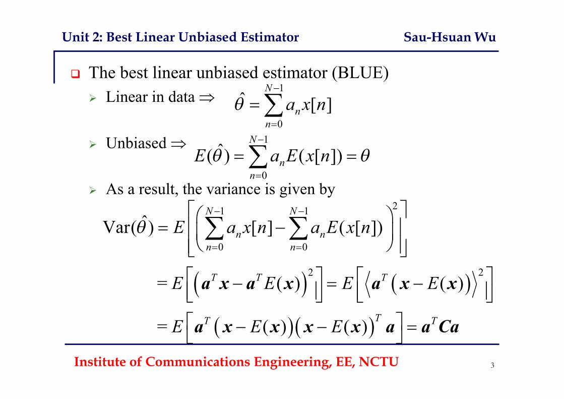
Using the method of Lagrangian multiplier, theLagrangian function becomes

J = aTCa + (aTs –1) Taking the gradient with respect to a gives

Setting this equal to the zero vector produces

Substituting this result back into the constraint yields

2J

Ca s

a

112

a C s

11

1 1

21 1, ,2T

optT T

C s

s C s as C s s C s



The corresponding variance is given by

The resultant estimator is

since E(x) = s To determine the BLUE, we only require knowledge of s or the scaled mean C, the covariancewhich are the first and second moments, but not the entire PDF

1 1

1 1 1

1TTopt opt T T T

s C C s

a Ca Cs C s s C s s C s

1

1ˆ

T

T

s C xs C s



Ex. x[n]= A + w[n], n=0,1,…,N-1 with var(w[n]) = n2

Since E(x[n]) = A s[n]=1 s = 1 Then

The min variance is

1

1ˆ

T

TA

1 C x1 C 1

1

20

1ˆvar( )1N

n n

A

2 10

2 21 0

1

2201

0 0 [ ]0 0 ˆwith A=

1

0 0

N

n nN

n nN

x n

C



Extension to a vector parameter If the parameters to be estimated are = [1,…,p]T

Then for the estimator to be linear

In matrix form, this is In order for to be unbiased

1

0

ˆ [ ], i=1,...,pN

i inn

a x n

1

ˆ , where [ ,..., ]Tp θ Ax A a a

θ̂

1 2

ˆ ( )

( ) p

E E

E

θ A x θ

x h h h θ Hθ

AH I



Similarly, we havex= E(x) + [x - E(x)]= H+w with w ~ N(0, C)

The optimization problem becomes

The Lagrangian function for each ai is given byJi = ai

TCai + (aiTH –ei

T) i with i = [1(i),…, p

(i)] Taking the gradient with respect to ai gives

Setting this equal to the zero vector produces

ˆ arg min trace subject toT A

θ ACA AH I

2ii i

i

J

Ca Hλ

a

112i i

a C Hλ



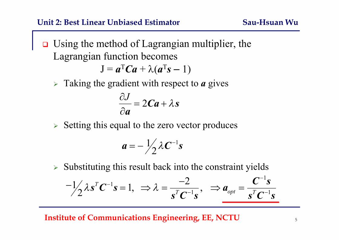
To satisfy the constraint of HTai = ei, we have

Eventually, we obtain

The estimator for i is

The corresponding variance is

1

11

12

2

T Ti i i

Ti i

H a H C Hλ e

λ H C H e

opt

11 1Ti i

a C H H C H e

opt opt

11ˆvar( ) T T Ti i i i i

a Ca e H C H e

opt

11 1ˆ T T T Ti i i

a x e H C H H C x



Now, if we put the estimators into a vector form

The corresponding covariance matrix is

where

Thus

Hence,

11 1ˆ T T θ H C H H C x



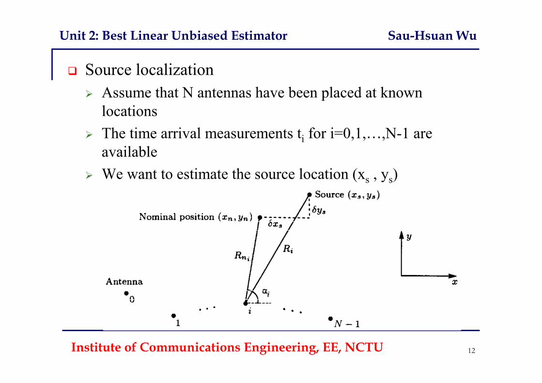
Source localization Assume that N antennas have been placed at known

locations The time arrival measurements ti for i=0,1,…,N-1 are

available We want to estimate the source location (xs , ys)



The measurements are modeled byti =T0 + Ri / c + i, i = 0,1,…,N-1

No assumptions are made about the PDF of i while we doknow its zero mean with variance 2

Let the position of the i-th antenna be (xi, yi)

Define = [xs , ys]T. ti is a function nonlinear in To apply the Gauss-Markov theorem, we assume a nominal

position (xn, yn) close to (xs , ys) is available We next update the position (xn+1, yn+1) to make it

approximate (xs , ys) sequentially. To this end, we require anestimate of

= [xs - xn, ys - yn]T = [xs , ys]T



Now use a first-order Taylor expansion of Ri (xs, ys) at(xn, yn)

and xs = xs-xn, ys = ys - yn

With this model we have

As defined in the figure

The model simplifies to

cos , sini i

n i n ii i

n n

x x y yR R

0cos sin

in i ii s s i

Rt T x y

c c c



Since is a known constant. Let i = ti -

In practice, knowledge of T0 would require accurate clocksynchronization between the source and the receiver

To avoid the synchronization requirement, it is customaryto consider time difference of arrivals (TDOA)

Generate the TDOAs asi = i - i-1, for i=1,2,…,N-1

0cos sini i

i s s iT x yc c

1 1 11 1

cos cos sin sini i i s i i s i ix yc c



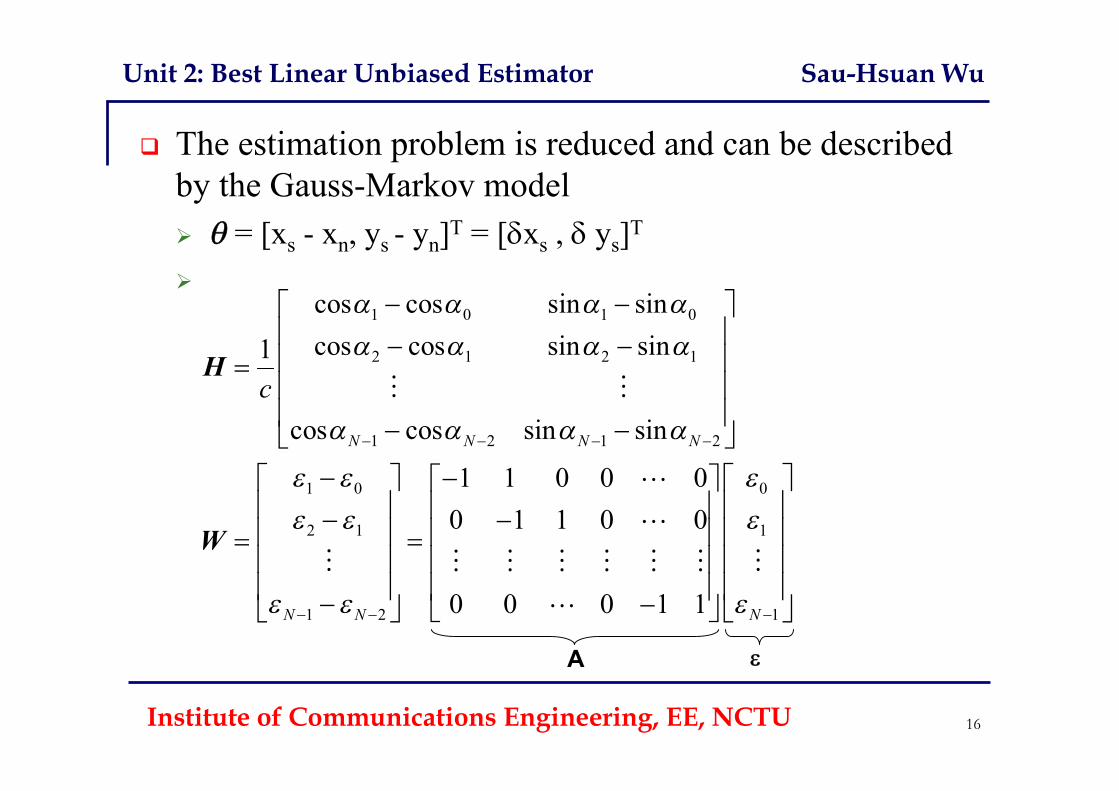
The estimation problem is reduced and can be describedby the Gauss-Markov model = [xs - xn, ys - yn]T = [xs , ys]T

1 0 1 0

2 1 2 1

1 2 1 2

1 0 0

2 1 1

1 2 1

cos cos sin sincos cos sin sin1

cos cos sin sin

1 1 0 0 00 1 1 0 0

0 0 0 1 1

N N N N

N N N

c

H

W

A



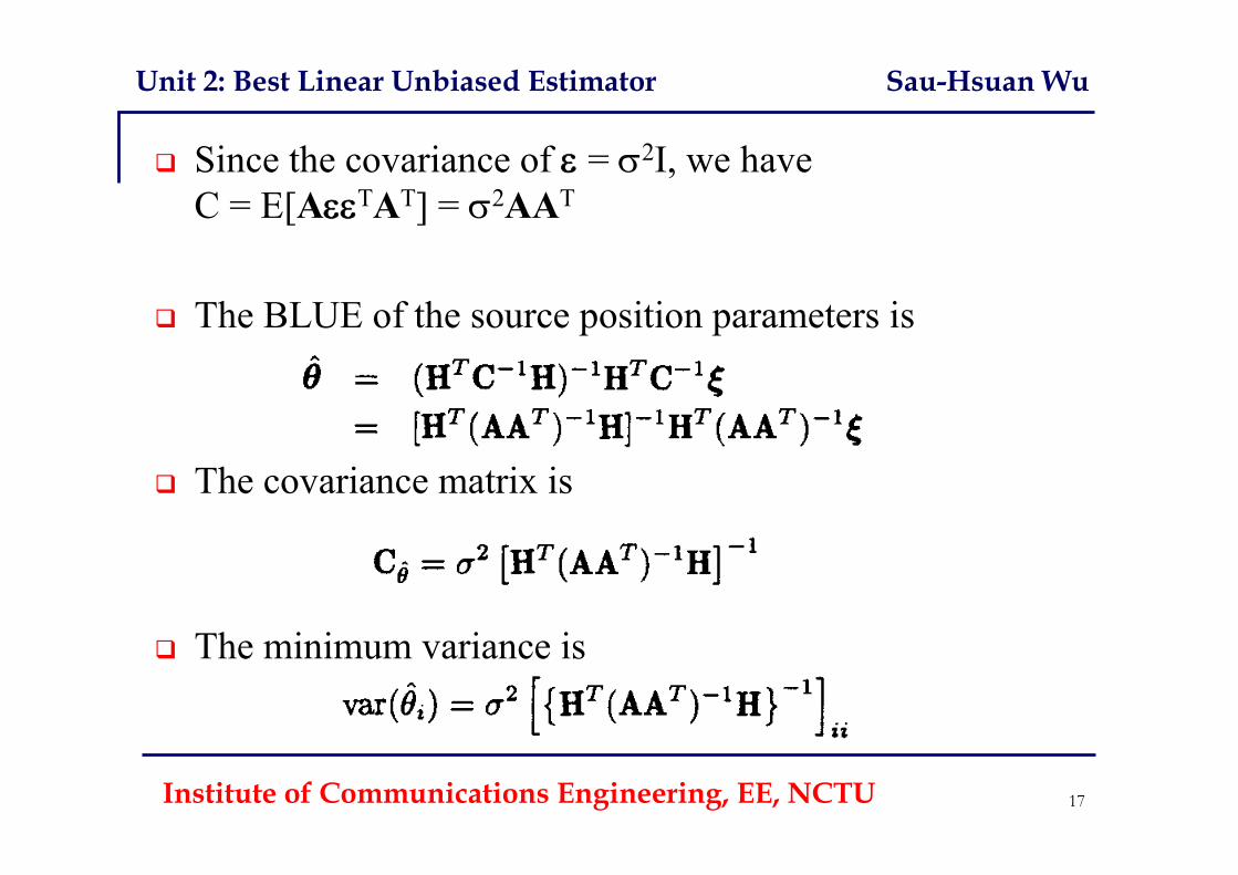
Since the covariance of = 2I, we haveC = E[ATAT] = 2AAT

The BLUE of the source position parameters is

The covariance matrix is

The minimum variance is



Suppose we have a three antenna linear array Then

For the best localization, we would like to be small d between antenna can be make large

Documents

Unit 2 Best Linear Unbiased Estimator (BLUE)