Unit 21 Conversation and speech in American English (Case study 5)

21.1 Introduction

This case study uses Biber’s (1988) multi-feature/multi-dimensional approach to genre analysis (see units 10.4 and 14.2) to compare the genres of conversation and speech in American English. The terms conversation and speech as used in this case study correspond to the demographically sampled and context-governed spoken data in the British National Corpus (BNC, see Aston and Burnard 1998:31). Conversation represents the type of communication we experience every day (Biber 1988: 10) whereas speech is produced in situations where there are few producers and many receivers (e.g. classroom lectures, sermons and political speeches). The result of this analysis will also be compared with the keyword analysis as discussed in units 10.11-10.12. We noted in case study 4 that, in modern British English, informal conversation and formal speech differ considerably in terms of the frequency and distribution of swear words. While it is possible to simply describe conversation as informal and speech as formal, it would be more accurate to consider the formal/informal or oral/literate distinction as a continuous dimension of variation distinguishing the two (cf. Biber 1988: 9). This however, requires the undertaking of a Biber-style analysis in order to explore how these two varieties of spoken language vary in these dimensions. It is this analysis that we will undertake in this unit. While our previous study of spoken English focused on modern British English, in this unit, we will switch our focus slightly and look instead at spoken American English, using the multi-feature/multi-dimensional (MF/MD) analytic framework established in Biber (1985, 1988) (see units 10.4 and 14.2). In this case study, we will also show you some advanced features of WordSmith (version 3), including concordance using file-based search patterns, wordlist and keyword. As Biber’s original framework involves sophisticated statistical analyses and is very time-consuming, the wordlist and keyword functions of WordSmith (referring to version 3 in this study) will be used to achieve an approximate effect of Biber’s multi-dimensional analysis (cf. Tribble 1999). For a fuller comparison of the two approaches to genre analysis, see Xiao and McEnery (2005). The major corpus resources used in this unit consist of the Santa Barbara Corpus of Spoken American English (SBCSAE) and two files (comm797.txt and comr797.txt) from the Corpus of Professional Spoken American English (CPSA) (see units 7.3 and 7.5 for a description of the two corpora). In order to contrast spoken data and written data, the section of academic prose (category J) from the Frown corpus (Frownj) is also included in this case study. Table 21.1 shows the data used in this unit. This unit consists of 6 sections. Unit 21.2 explains the functions of 58 linguistic features and designs a set of search algorithms for extracting their frequencies; unit 21.3 calculates the basic statistics for each linguistic feature, including minimum/maximum frequency, range, mean and standard deviation (see unit 6.3); unit 21.4 compares the three genres alongside 7 dimensions while unit 21.5 presents a keyword analysis using wordsmith; finally unit 21.6 concludes the unit.

Table 21.1 Corpus data Genre Corpus Sampling date No. of texts No. of tokens No. of tokens

by genre Conversation SBCSAE 1988-1993 31 135834 135834

SBCSAE 1988-1993 12 46312 Speech CPSA 1997 2 157498

203810

Academic prose Frownj 1991-1992 80 166169 166169 Total 125 505813

21.2 Salient linguistic features

The 67 linguistic features Biber (1988) used are all functionally related and have been studied extensively. Biber (1998: 223-245) provides a good review of the functions of each of these linguistic features. The salient linguistic features associated with each of the seven factors (Biber 1988: 102-103) are given in Table 21.2. Note that in the table (Factor +3), WH relative clauses on object and subject positions are kept together to make presentation easier. For the same reason, THAT relative clauses (Factor +6) refer to those on either object or subject positions. Combinations of similar features like these reduce the number of linguistic features under consideration to 58.

Table 21.2 Factorial structures of 7 dimensions Factor Linguistic features +1 (1) private verbs, (2) THAT deletion, (3) contraction, (4) present tense verbs, (5) 2nd

person pronouns, (6) DO as pro-verb, (7) analytic negation, (8) demonstrative pronouns, (9) general emphatics, (10) 1st person pronouns, (11) pronoun IT, (12) BE as main verb, (13) causative subordination, (14) discourse markers, (15) indefinite pronouns, (16) general hedges, (17) amplifiers, (18) sentence relatives, (19) WH questions, (20) possibility modals, (21) non-phrasal coordination, (22) WH clauses, (23) final prepositions

-1 (24) other nouns, (25) word length, (26) prepositions, (27) type/token ratio, (28) attributive adjectives

+2 (29) past tense verbs, (30) 3rd person pronouns, (31) perfect aspect verbs, (32) public verbs, (33) synthetic negation, (34) present participial clauses

+3 (35) WH relative clauses, (36) pied piping constructions, (37) phrasal coordination, (38) nominalizations

-3 (39) time adverbials, (40) place adverbials, (41) other adverbs +4 (42) infinitives, (43) prediction modals, (44) suasive verbs, (45) conditional

subordination, (46) necessity modals, (47) split auxiliaries +5 (48) conjuncts, (49) agentless passives, (50) past participial clauses, (51) BY-passives,

(52) past participial WHIZ deletions, (53) other adverbial subordinators +6 (54) THAT clauses as verb complements, (55) demonstratives, (56) THAT relative

clauses, (57) THAT clauses as adjective complements +7 (58) SEEM/APPEAR As can be seen from the table, some factorial structures include factors with negative loadings. Biber observes that features with positive loadings on a dimension co-occur frequently whereas features with negative loadings occur together. The dimension score of a text is computed by adding together the factor score of each feature with a positive loading, and then subtracting the factor score of each feature, if any, with a negative loading. The dimension score of a genre is the mean of the factor scores of the texts within the genre. We will show you how to compute the factor score in unit 21.4. But first we need to explain the functions of salient linguistic features and find a way to extract their frequency counts in the corpus.

The features with positive loadings on Factor 1, which are ‘characterized as verbal, interactive, affective, fragmented, reduced in form, and generalized in content’, ‘can be associated in one way or another with an involved, non-informational focus’ (Biber 1988: 105). Conversely, high frequencies of features with negative weights are associated with a high informational focus and a careful integration of information in a text. The features with salient positive weights on Factor 2 can all be used for narrative purposes (Biber 1988: 92), though narrative discourse depends heavily on the past tense and perfect aspect verbs (Biber 1988: 109). Alongside Factor 3, features with positive loadings include WH relative clauses, phrasal coordination and nominalization. Relativization specifies ‘the identity of referents within a text in an explicit and elaborated manner, so that the addressee will have no doubt as to the intended referent’ while ‘the co-occurrence of phrasal coordination and nominalizations with these relativization features indicates that referentially explicit discourse also tends to be integrated and informational’ (Biber 1988: 110). The two features with negative weights, time and place adverbials, on the other hand, depend crucially on the addressee for text-internal references. The features associated with Factor 4 function together to mark persuasion, whether overt marking of the addresser’s own viewpoint, or an assessment of the advisability or likelihood of an event presented to persuade the addressee (cf. Biber 1988: 111). The features associated with Factor 5 are conjuncts, main/subordinate passive constructions and adverbial subordinators. Discourse with a high frequency of passives is typically abstract and technical in content, as well as formal in style. This type of discourse is generally characterized by complex logical relations, which are achieved by conjuncts and adverbial subordinators (cf. Biber 1988: 112). Features with salient positive weights on Factor 6 function to mark informational elaboration in discourse that is informational but produced under real-time conditions (Biber 1988: 113-114). Factor 7 only has one salient positive feature, SEEM/APPEAR. SEEM and APPEAR mark perception rather than assertion of fact and thus mark an assertion as uncertain. They are typically used in academic discourse as a downtoner to qualify the extent to which an assertion is known (Biber 1988: 114). Biber (1988: 211-245) proposed a set of algorithms for the automatic identification of the 67 linguistic features he used. As the data he used was annotated differently from ours, Biber’s algorithms do not apply to our data. We have designed search patterns suitable for corpora POS tagged by CLAWS using the BNC C7 tagset (see unit 4.4.1). As the normal concordance function of WordSmith allows only 15 search phrases as long as they are limited to 80 characters, including the symbol / (‘or’), some of our search phrases are file-based, i.e., saved as a text file. This approach allows up to 500 search patterns. You will need to download the file-based search patterns from our companion website. We assume that you have placed these files in the same file folder as WordSmith. In the remainder of this section, we will show you, through corpus examples, what we are looking for with regard to each of the linguistic features listed in Table 21.2. You will find all of the search patterns on our companion website. Dimension 1: Informational versus involved production (23 features with positive loadings and five with negative loadings)

Features with positive loadings: (1) private verbs: All morphological forms of the following verbs: anticipate, assume,

believe, conclude, decide, demonstrate, determine, discover, doubt, estimate, fear,

feel, find, forget, guess, hear, hope, imagine, imply, indicate, infer, know, learn, mean, notice, prove, realize, recognize, remember, reveal, see, show, suppose, think, understand;

(2) THAT deletion: e.g., I think [that] it’s so funny. (3) contraction: n’t, ’ll, ’d, ’m, ’re, ’ve, ’s (excluding possessive form); (4) present tense verbs: All base forms and third person singular present verb forms. (5) 2nd person pronouns: you, your, yourself, yourselves, yours; (6) DO as a pro-verb: e.g., You did that? (7) analytic negation: not, n’t; (8) demonstrative pronouns: this, that, these and those (not followed by a noun); (9) general emphatics: for sure, a lot, such a, real, so, just, really, most, more and DO

+ verb; (10) 1st person pronouns: I, my, our, myself, ourselves, mine and ours; (11) pronoun IT: it; (12) BE as a main verb (excluding BE as an auxiliary): e.g., You are right. (13) causative subordination: because; (14) discourse markers: well, anyway, anyways, anyhow; (15) indefinite pronouns: e.g., none, one, anyone, someone, somebody, anybody,

nobody, everything, nothing; (16) general hedges: about (not as a preposition), something like, more or less, almost,

maybe, sort of and kind of (excluding sort and kind as true nouns); (17) amplifiers: absolutely, altogether, completely, enormously, entirely, extremely,

fully, greatly, highly, intensely, perfectly, strongly, thoroughly, totally, utterly and very;

(18) sentence relatives: e.g., The present book, which is the first… (19) WH questions: e.g., What is it? (20) possibility modals: can, could, may and might (including contracted forms); (21) non-phrasal coordination: e.g., Yeah, and it has. (22) WH clauses: e.g., You know what I mean. (23) final prepositions: e.g., Where did you get it from? Features with negative loadings: (24) other nouns: All noun forms excluding nominalizations (see 38 below); (25) word length: (WordSmith wordlist function: average word length) (26) prepositions: All prepositions like at, by, in and of; (27) type/token ratio: (WordSmith wordlist function: standardized type/token ratio); (28) attributive adjectives: e.g., young girl and new regulatory requirements. Dimension 2: Narrative versus non-narrative concerns (Six linguistic features, all with positive loadings) (29) past tense verbs: All past tense verbs; (30) 3rd person pronouns: she, he, they, her, him, them, his, its, hers, their, theirs,

himself, herself and themselves (including contractions); (31) perfect aspect verbs: e.g., That hasn’t finished. (32) public verbs: All morphological forms of the following verbs: acknowledge,

admit, agree, assert, claim, complain, declare, deny, explain, hint, insist, mention, proclaim, promise, protest, remark, reply, report, say, suggest, swear and write;

(33) synthetic negation: neither, nor and no (excluding no as a response); (34) present participial clauses: e.g., So, you got this Oscar there, swimming there in

the tank.

Dimension 3: explicit versus situation-dependent reference (Four features with positive loadings and three with negative loadings)

Features with positive loadings: (35) WH relative clauses: e.g., You know the little folks who live above me. (36) pied piping constructions: e.g., the problems with which he is concerned; (37) phrasal coordination: e.g., economic and social conditions, racism and sexism,

pick and choose; (38) nominalizations: All nouns ending in -tion, -ment, -ness, -ity (including plural

forms); Features with negative loadings: (39) time adverbials: All adverbs of time; (40) place adverbials: All adverbs of place; (41) other adverbs: All adverbs minus all totals of hedges, amplifiers, downtoners,

place adverbials and time adverbials Dimension 4: Overt expression of persuasion (Six linguistic features, all with positive loadings) (42) infinitives: to + base form of a verb (may be separated by one or two adverbs); (43) prediction modals: will, shall and would (including contractions); (44) suasive verbs, including all morphological forms of the following verbs: agree,

arrange, ask, beg, command, decide, demand, grant, insist, instruct, ordain, pledge, pronounce, propose, recommend, request, stipulate, suggest and urge;

(45) conditional subordination: if and unless (46) necessity modals: ought, should and must; (47) split auxiliaries: e.g., You’re just saying that. Dimension 5: Abstract versus non-abstract information (Six linguistic features, all with positive loadings) (48) conjuncts: alternatively, altogether, consequently, conversely, eg, e.g., else,

furthermore, hence, however, i.e., instead, likewise, moreover, namely, nevertheless, nonetheless, notwithstanding, otherwise, rather, similarly, that is, therefore, thus, viz, in (comparison, contrast, particular, addition, conclusion, consequence, sum, summary, any event, any case, other words), for example (instance), by contrast (comparison), as a result (consequence), on the contrary (other hand);

(49) agentless passives: e.g., And this book was written in nineteen ten. (50) past participial clauses: e.g., This problem, combined with administrative failure

to meet… (51) BY-passives: e.g., It is shared by preacher and audience. (52) past participial WHIZ deletions: e.g. tests designed for old age groups; (53) other adverbial subordinators: since, while, whilst, whereupon, whereas, whereby,

such that, so that, inasmuch as, forasmuch as, insofar as, insomuch as, as long as and as soon as.

Dimension 6: Online informational elaboration (Four linguistic features, all with positive loadings)

(54) THAT clauses as verb complements: e.g., So he knew that the oil was leaking? (55) demonstratives: this, that, these and those followed by a noun; (56) THAT relative clauses: e.g., In fact, I eat stuff that he doesn’t eat. (57) THAT clauses as adjective complements: e.g., I’m just happy that I beat you. Dimension 7: Academic hedging (58) SEEM/APPEAR: all morphological forms of SEEM and APPEAR. While some of the patterns we have devised may only extract typical instances and some of them may even generate false matches due to tagging errors, the same patterns are applied to all corpus files. Hence we consider the results for the different genres to be comparable and sufficiently reliable, in spite of the small margin of error associated with our pattern matching procedure, as it is assumed that the errors are distributed evenly across the files.

21.3 Basic statistical data from the corpus

This section demonstrates how to extract the frequencies of salient linguistic features and compute the mean, range and standard deviation of each of the features in the whole corpus (see unit 6.3 for a discussion of these statistics). We will use the mean and standard deviation to compute the factor scores of linguistic features. To begin the computation of the factor scores, we need to extract the frequencies of each feature from the corpus using WordSmith and the search patterns established in unit 21.2. Note that in this section, all frequencies are normalized to a common 1,000-word basis to ensure comparability between files of different sizes. We have formatted our corpus data to place metadata in angled brackets so that it can be ignored in concordancing by activating Tags to ignore <*> in WordSmith Settings. Ensure that you have made this change to settings before proceeding. Then load WordSmith with all of the 125 corpus files by selection File – Choose texts in the main menu. To find out the minimum/maximum frequencies, mean, range and standard deviation for private verbs in the corpus, do the following:

1. Start the concordance function of WordSmith, type in the path of the file containing search patterns of private verbs, and press Go Now, as shown in Fig. 21.1.

2. You will be led to the concordance window as shown in Fig. 21.2. Press on the toolbar to show the distribution of private verbs across files (Fig. 21.3). The left panel of the dispersion window shows the number of files containing private verbs, filenames, file sizes in tokens, raw frequencies and normalized frequencies (per 1,000 words) while the right panel shows the location of the matches in each file. Note that if a linguistic feature is absent in some files, the number of files shown here may be fewer than the number of files you loaded. Of these we are only interested in the normalized frequencies. The files are arranged in descending order on the basis of normalized frequencies. You can click your mouse on the icon in the toolbar or press F6 on your keyboard to re-sort the files into the order you wish. As we will see later, it is a good idea to re-sort filenames in alphabetical order. While you can type the normalized frequencies into the data editor of SPSS one by one manually, you can also use the copy and paste function provided by Windows. To select the data needed, click your mouse on the filename of the first file, hold down

the SHIFT key on your keyboard, and move the right arrow key until File, Words, Hits and per 1,000 are highlighted. Then while still holding down the SHIFT key, move the down arrow key until the whole left panel is highlighted. Press Ctrl+C to make a copy.

3. Start the SPSS statistics package (see case study 2) and define five variables as shown in Fig. 21.4.

4. Select the Data View label in the bottom left corner of the window, select the first field under the variable file_no by clicking your mouse on it, and press Ctrl+V to paste the data into the SPSS data editor, as shown in Fig. 21.5.

Fig. 21.1 The file-based search pattern Fig. 21.2 A concordance of private verbs

Fig. 21.3 The distribution of private verbs Fig. 21.4 Defining variables with SPSS

Fig. 21.5 Pasting data into SPSS Fig. 21.6 Computing basic statistics using SPSS

Note that the numbers of words, as well as the counts of hits that contain a comma, are not shown in the data editor because we have defined these variables as numerical, which cannot include commas. But this is not a problem. All we need is the frequencies per 1,000 tokens.

Fig. 21.7 Selecting variable(s) Fig. 21.8 Selecting the parameters

Fig. 21.9 Basic statistics relating to private verbs

5. Select Analyze → Descriptive Statistics → Descriptives as shown in Fig. 21.6.

6. Select the variable per1000 as shown in Fig. 21.7.

7. Press Options and select Range (Mean, Std deviation, minimum and maximum are selected by default). Press Continue to return to the previous window (Fig. 21.8). Press OK.

8. You will be taken to the output window as shown in Fig. 21.9. Here you can find the basic descriptive statistics of private verbs in the corpus. The above steps provide a standard procedure for computing the basic statistics of linguistic features. However, some features may require more complicated operations. For example, to extract the instances of THAT deletion, you will need to search the corpus eight times and save each concordance as a separate file, and merge two files at one time (by selecting File → Merge from the menu of Concord) until all of the eight files are combined into one concordance list. As some of the linguistic features are very frequent (e.g. 1st person pronouns, present tense verbs, attributive adjectives, other nouns, other adverbs, prepositions), WordSmith ignores all matches beyond a ceiling of 16368. If the program shows 16,368 matches, the actual number of matches may be greater. If you have not yet done so, select the Concord label in WordSmith Settings and define Entities wanted to be 16,368. In order to extract all examples in such cases, you will need to load part of the corpus files and copy the data from the dispersion window to the SPSS data editor several times. For example, the single file comr797.txt (speech) needs to be split into two halves to extract the frequencies of other nouns. Note, however, that it is essential

that you clear previous files whenever you choose fresh texts, otherwise the new texts will simply be added to the old. To extract the frequency of other adverbs, it is necessary to discover the count of *_R*, and then subtract the counts of hedges, amplifiers, downtoners, place adverbials and time adverbials. Note that as the search pattern for hedges includes something like, which is not tagged as adverbial (R*), the count of this expression should not be included. You can use c:\wsmith\hedge1.txt as the search pattern for hedges in this case. When you copy and paste data from the concordance dispersion window to the SPSS data editor, it is necessary to re-sort filenames alphabetically and make adjustments in the SPSS data editor so that the frequencies from each file appear on the same row before doing the subtractions. The word length and type/token ratio can be obtained by using the wordlist function of WordSmith. As the program by default treats the underscore linked part-of-speech tag (e.g. and_CC) as the suffix (i.e. ANDCC) as well as a separate token (i.e. CC), we need to adjust the settings to allow the program to treat the tagged corpus files appropriately. Make sure, however, that you restore the tag setting after you make a wordlist for the corpus; otherwise, the search algorithms will not work. 9. Select the Tags label in WordSmith Settings and define the tag to ignore as _*, as shown in Fig. 21.10.

10. Click on Only Part of File, activate Sections to Cut and define the start mark as the opening bracket < and the end mark as the closing bracket > (Fig. 21.11). This definition achieves the same effect as ignoring tag <*>. Press OK twice.

11. Load all of the 125 files (again, remember to clear previous files before this operation).

12. Select Tools → Wordlist. Press the start button on the toolbar, and you will see the Getting started window. Make sure that the number of files chosen is 125. Press Make a wordlist now (Fig. 21.12).

13. You will see three wordlists are made. Wordlist (A) is an alphabetically ordered list, wordlist (F) is a frequency ordered list and wordlist (S) shows the basic statistics such as type/token ratio and average word length (Fig. 21.13).

14. Select wordlist (S), and type the Ave word length for 125 files into the SPSS data editor to compute the minimum/maximum frequency, mean, range and standard deviation. Do the same for Standardised Type/Token Ratio.

Fig. 21.10 Adjusting tag setting Fig. 21.11 Defining sections to cut

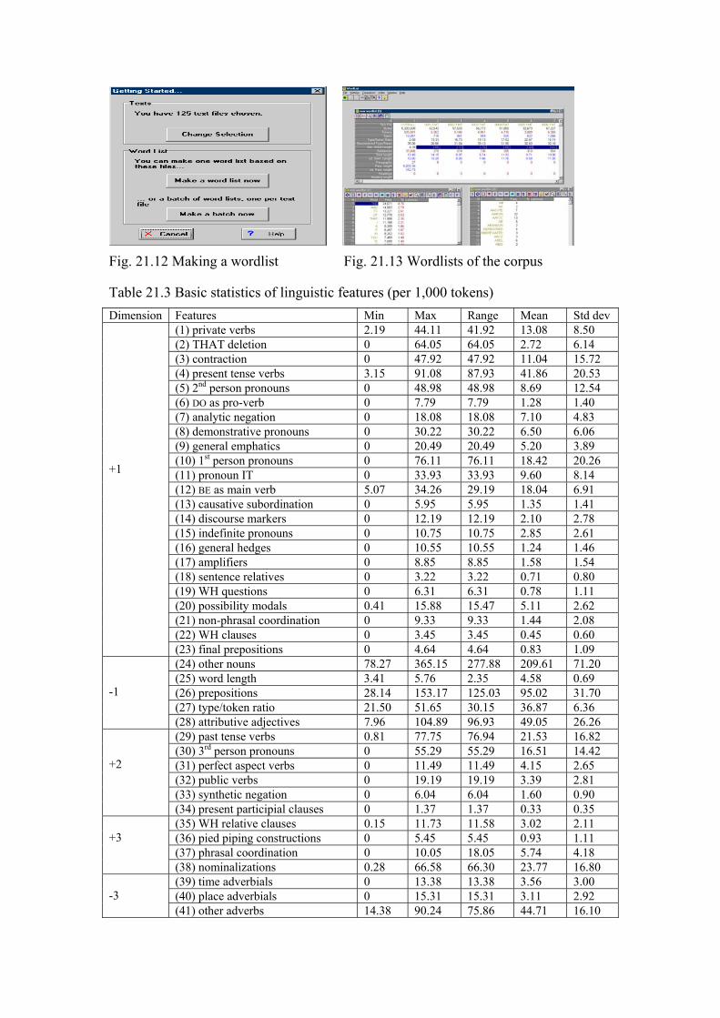
Fig. 21.12 Making a wordlist Fig. 21.13 Wordlists of the corpus

Table 21.3 Basic statistics of linguistic features (per 1,000 tokens) Dimension Features Min Max Range Mean Std dev

(1) private verbs 2.19 44.11 41.92 13.08 8.50 (2) THAT deletion 0 64.05 64.05 2.72 6.14 (3) contraction 0 47.92 47.92 11.04 15.72 (4) present tense verbs 3.15 91.08 87.93 41.86 20.53 (5) 2nd person pronouns 0 48.98 48.98 8.69 12.54 (6) DO as pro-verb 0 7.79 7.79 1.28 1.40 (7) analytic negation 0 18.08 18.08 7.10 4.83 (8) demonstrative pronouns 0 30.22 30.22 6.50 6.06 (9) general emphatics 0 20.49 20.49 5.20 3.89 (10) 1st person pronouns 0 76.11 76.11 18.42 20.26 (11) pronoun IT 0 33.93 33.93 9.60 8.14 (12) BE as main verb 5.07 34.26 29.19 18.04 6.91 (13) causative subordination 0 5.95 5.95 1.35 1.41 (14) discourse markers 0 12.19 12.19 2.10 2.78 (15) indefinite pronouns 0 10.75 10.75 2.85 2.61 (16) general hedges 0 10.55 10.55 1.24 1.46 (17) amplifiers 0 8.85 8.85 1.58 1.54 (18) sentence relatives 0 3.22 3.22 0.71 0.80 (19) WH questions 0 6.31 6.31 0.78 1.11 (20) possibility modals 0.41 15.88 15.47 5.11 2.62 (21) non-phrasal coordination 0 9.33 9.33 1.44 2.08 (22) WH clauses 0 3.45 3.45 0.45 0.60

+1

(23) final prepositions 0 4.64 4.64 0.83 1.09 (24) other nouns 78.27 365.15 277.88 209.61 71.20 (25) word length 3.41 5.76 2.35 4.58 0.69 (26) prepositions 28.14 153.17 125.03 95.02 31.70 (27) type/token ratio 21.50 51.65 30.15 36.87 6.36

-1

(28) attributive adjectives 7.96 104.89 96.93 49.05 26.26 (29) past tense verbs 0.81 77.75 76.94 21.53 16.82 (30) 3rd person pronouns 0 55.29 55.29 16.51 14.42 (31) perfect aspect verbs 0 11.49 11.49 4.15 2.65 (32) public verbs 0 19.19 19.19 3.39 2.81 (33) synthetic negation 0 6.04 6.04 1.60 0.90

+2

(34) present participial clauses 0 1.37 1.37 0.33 0.35 (35) WH relative clauses 0.15 11.73 11.58 3.02 2.11 (36) pied piping constructions 0 5.45 5.45 0.93 1.11 (37) phrasal coordination 0 10.05 18.05 5.74 4.18

+3

(38) nominalizations 0.28 66.58 66.30 23.77 16.80 (39) time adverbials 0 13.38 13.38 3.56 3.00 (40) place adverbials 0 15.31 15.31 3.11 2.92

-3

(41) other adverbs 14.38 90.24 75.86 44.71 16.10

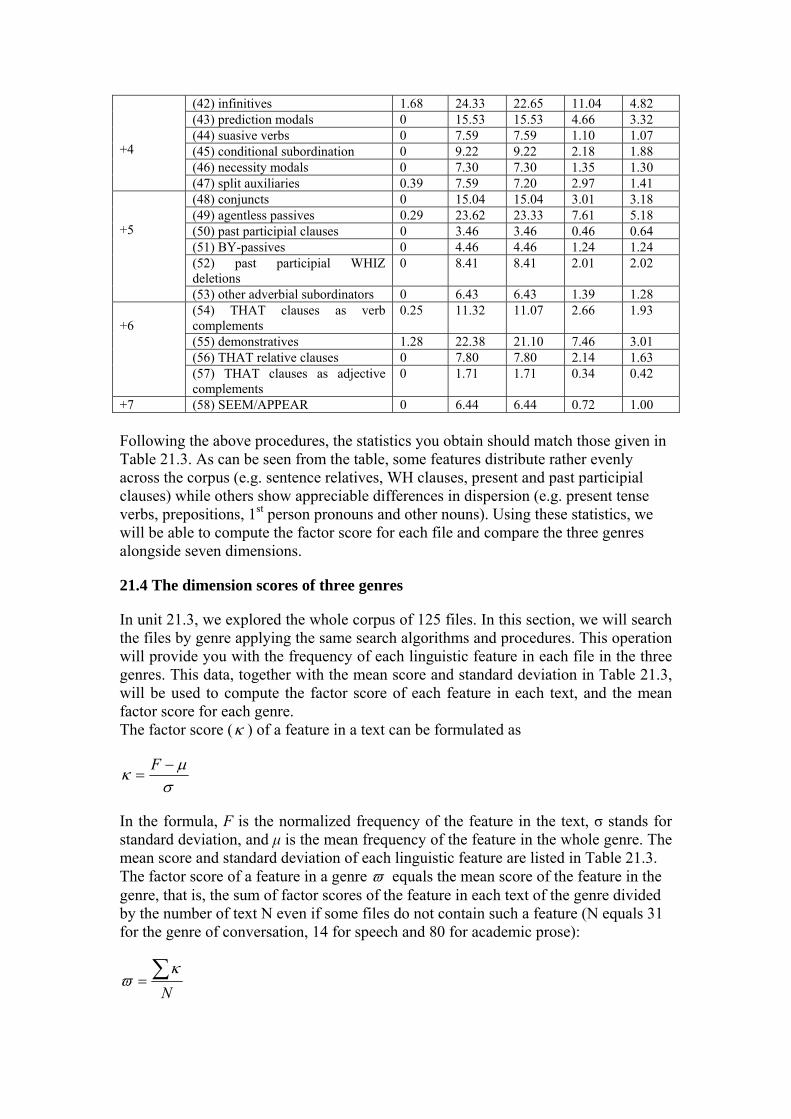
(42) infinitives 1.68 24.33 22.65 11.04 4.82 (43) prediction modals 0 15.53 15.53 4.66 3.32 (44) suasive verbs 0 7.59 7.59 1.10 1.07 (45) conditional subordination 0 9.22 9.22 2.18 1.88 (46) necessity modals 0 7.30 7.30 1.35 1.30

+4

(47) split auxiliaries 0.39 7.59 7.20 2.97 1.41 (48) conjuncts 0 15.04 15.04 3.01 3.18 (49) agentless passives 0.29 23.62 23.33 7.61 5.18 (50) past participial clauses 0 3.46 3.46 0.46 0.64 (51) BY-passives 0 4.46 4.46 1.24 1.24 (52) past participial WHIZ deletions

0 8.41 8.41 2.01 2.02

+5

(53) other adverbial subordinators 0 6.43 6.43 1.39 1.28 (54) THAT clauses as verb complements

0.25 11.32 11.07 2.66 1.93

(55) demonstratives 1.28 22.38 21.10 7.46 3.01 (56) THAT relative clauses 0 7.80 7.80 2.14 1.63

+6

(57) THAT clauses as adjective complements

0 1.71 1.71 0.34 0.42

+7 (58) SEEM/APPEAR 0 6.44 6.44 0.72 1.00 Following the above procedures, the statistics you obtain should match those given in Table 21.3. As can be seen from the table, some features distribute rather evenly across the corpus (e.g. sentence relatives, WH clauses, present and past participial clauses) while others show appreciable differences in dispersion (e.g. present tense verbs, prepositions, 1st person pronouns and other nouns). Using these statistics, we will be able to compute the factor score for each file and compare the three genres alongside seven dimensions.

21.4 The dimension scores of three genres

In unit 21.3, we explored the whole corpus of 125 files. In this section, we will search the files by genre applying the same search algorithms and procedures. This operation will provide you with the frequency of each linguistic feature in each file in the three genres. This data, together with the mean score and standard deviation in Table 21.3, will be used to compute the factor score of each feature in each text, and the mean factor score for each genre. The factor score (κ ) of a feature in a text can be formulated as

σμκ −

=F

In the formula, F is the normalized frequency of the feature in the text, σ stands for standard deviation, and μ is the mean frequency of the feature in the whole genre. The mean score and standard deviation of each linguistic feature are listed in Table 21.3. The factor score of a feature in a genre ϖ equals the mean score of the feature in the genre, that is, the sum of factor scores of the feature in each text of the genre divided by the number of text N even if some files do not contain such a feature (N equals 31 for the genre of conversation, 14 for speech and 80 for academic prose):

N∑= κ

ϖ

The dimension score of a genre can be obtained by adding together the mean factor scores of all features with positive weights on a factor and then subtracting the mean factor scores of all features with negative weights on the same factor:

∑= ϖω

For example, the factor score of Dimension 1 equals the sum of mean factor scores of all features that appear under the label +1 less the total of mean factor scores of the features that appear under the label –1. Note that the positive or negative sign preceding a value should be retained so that – (–1) means +1. For example, suppose for the genre of academic prose the mean factor scores of the four features with positive weights on Factor 3 are –0.57, +0.53, +0.51 and +0.60 while those for features with negative weights are –0.44, –0.43 and –0.51, the dimension score of Factor 3 for academic prose should be +2.45 rather than –0.31. The three formulae presented above may involve thousands of arithmetic operations. We wrote a simple program to do the boring calculations using the output of WordSmith. If you do not wish to do the calculations by yourself, you can download the program from our companion website (see the readme file accompanying the program for details of how to use it). The dimension scores for Factors 1-7 computed for the genres of conversation, speech and academic prose are given in Tables 21.4-21.10. As can be seen in Table 21.4, with the exception of THAT deletion, amplifiers and sentence relatives, the features with positive loadings on Factor 1 have greater scores in conversation than in speech. Similarly, the absolute values of the scores of features with negative weights on Factor 1 are greater in conversation than in speech. The contrast between academic prose and conversation is even more marked. Dimension 1 is a fundamental parameter to mark the relative ‘oralness’ or ‘literateness’ of a genre (Biber 1988: 108). Therefore, conversation, which has an involved, interactive focus and is subject to real-time production constraints, is the most ‘oral’ of the three genres in this study. In contrast, academic prose is the most ‘literate’ of the three in that it is characterized by careful editing possibilities and informational density. Table 21.5 shows that alongside Dimension 2, speech is more narrative than academic prose and conversation. This is unsurprising when one considers that academic prose has its focus on exposition rather than narration whereas conversation, while it may involve narration, has an interactive and affective focus. Alongside Dimension 3, conversation and speech are quite similar in that both genres make explicit context-independent references, though to varying degrees (Table 21.6). In contrast, academic prose tends to make context dependent references. This feature is explicable in terms of the greater number of opportunities that writing affords one to undertake careful editing. Such opportunities are atypical of spontaneous speech. As can be seen in Table 21.7, all of the three genres under consideration are related to persuasion. Speech is the most persuasive while academic prose is the least persuasive. Conversation may involve persuasion, but to a lesser extent than speech. In terms of Dimension 5, academic prose is much more technical and abstract than speech and conversation. Surprisingly, our data shows that conversation is more abstract than speech, which runs contrary to one’s intuition (Table 21.8).

Table 21.4 Dimension 1 (Informational versus involved production) Dimension Linguistic Private Public Academic

feature conversation speech prose Private verbs +1.36 +0.37 -0.59 THAT deletion +0.19 +0.27 +0.03 Contractions +1.54 +0.68 -0.14 Present tense verbs +1.20 +0.67 -0.58 2nd person pronouns +1.44 +0.60 -0.10 DO as pro-verb +1.06 +0.59 -0.15 Analytic negation +1.32 +0.61 -0.60 Demonstr pronoun +1.28 +0.80 -0.58 Emphatics +1.26 +0.19 -0.49 1st person pronoun +1.30 +0.90 -0.51 Pronoun IT +1.40 +0.47 -0.60 BE as main verb +0.94 +0.69 -0.49 Caus subordination +0.73 +0.78 -0.05 Discourse markers +1.36 +0.45 -0.61 Indefinite pronouns +1.25 +0.43 -0.38 Hedges +1.08 +0.41 -0.14 Amplifiers -0.20 +0.84 +0.11 Sentence relative -0.22 +0.04 +0.49 WH questions +0.92 +0.88 -0.004 Possibility modals +0.35 +0.03 -0.14 Non-phrasal coordination +1.03 +0.49 -0.19 WH clauses +1.09 -0.83 -0.33

+1

Final prepositions +1.09 +0.76 -0.05 Other nouns -1.12 -0.72 +0.66 Word length -1.35 -0.71 +0.66 Prepositions -1.43 -0.64 +0.67 Type/token ratio -1.05 -0.60 +0.53

-1

Attributive adjectives -1.24 -0.84 +0.63 Dimension 1 factor score: +1– (–1) +28.96 +14.63 -9.24

Table 21.5 Dimension 2 (Narrative versus non-narrative concerns) Linguistic feature

Private conversation

Public speech

Academic prose

Past tense verbs +0.58 +0.49 -0.31 3rd person pronouns +0.86 +0.75 -0.44 Perfect aspect verbs -0.04 +0.12 +0.05 Public verbs +0.39 +1.13 -0.26 Synthetic negation -0.80 -0.90 -0.09 Present participle clause +0.21 +0.41 +0.44 Mean factor score +1.20 +2.00 -0.61

Table 21.6 Dimension 3 (Explicit versus situation-dependent reference) Dimension Linguistic

Feature Private conversation

Public speech

Academic prose

WH relative clause -0.99 -0.84 -0.57 Pied piping constructs -0.13 -0.33 +0.53 Phrasal coordination -0.98 -0.64 +0.51

+3

Nominalization -1.25 -0.66 +0.60 Time adverbials +1.06 +0.90 -0.44 Place adverbials +1.12 +0.84 -0.43

-3

Other adverbs +1.10 +0.50 -0.51 Dimension 3 mean factor score: +3-(-3) -6.63 -4.71 +2.45

Table 21.7 Dimension 4 (Overt expressions of persuasion) Linguistic Private Public Academic

feature conversation speech prose Infinitives -0.14 +0.39 +0.10 Predication modals +0.82 +0.74 -0.38 Suasive verbs -0.21 +0.22 +0.30 Conditional sub. +0.59 +0.53 -0.15 Necessity modals -0.14 -0.15 +0.31 Split auxiliaries -0.18 -0.40 +0.14 Mean factor score +0.74 +1.33 +0.32

Table 21.8 Dimension 5 (Abstract versus non-abstract information) Linguistic feature

Private conversation

Public speech

Academic prose

Conjuncts -0.48 -0.52 +0.48 Agentless passives -0.11 -0.42 +0.50 Past participial clause -0.11 -0.26 +0.52 BY-passives -0.13 -0.46 +0.52 Past participial WHIZ deletion -0.41 -0.59 +0.51 Other adverbial subordination -0.52 -0.52 +0.37 Mean factor score -1.76 -2.77 +2.9

Table 21.9 Dimension 6 (Online informational elaboration) Linguistic feature

Private conversation

Public Speech

Academic prose

THAT clause as verb complements

-0.64 -0.14 +0.23

Demonstratives +0.06 +0.74 -0.15 THAT relative clauses -0.62 +0.44 +0.23 THAT clauses as adj. complements

+0.01 +0.19 +0.53

Mean factor score -1.19 +1.23 +0.84

Table 21.10 Dimension 7 (Academic hedging) Linguistic feature

Private conversation

Public speech

Academic prose

SEEM/APPEAR -0.05 +0.03 +0.40 Mean factor score -0.05 +0.03 +0.40

Table 21.11 Dimension scores of the three genres Dimension Conversation Speech Academic prose F-E value Sig. level 1 +28.96 +14.63 -9.24 2 +1.20 +2.00 -0.61 3 +1.10 -4.47 +2.45 4 +0.74 +1.33 +0.32 5 -1.76 -2.77 +2.90 6 -1.19 +1.23 +0.84 7 -0.05 +0.03 +0.40

32.47

<0.001

Table 21.9 shows that speech has the greatest score for Dimension 6, which marks the degree of online informational elaboration under strict real-time conditions. As conversation does not have an informational focus, it does not need stylistic elaboration. While academic prose is an informationally dense genre that needs elaboration, it is not subject to strict real-time conditions. Rather it is produced under circumstances that allow precise lexical choice and careful structural elaboration.

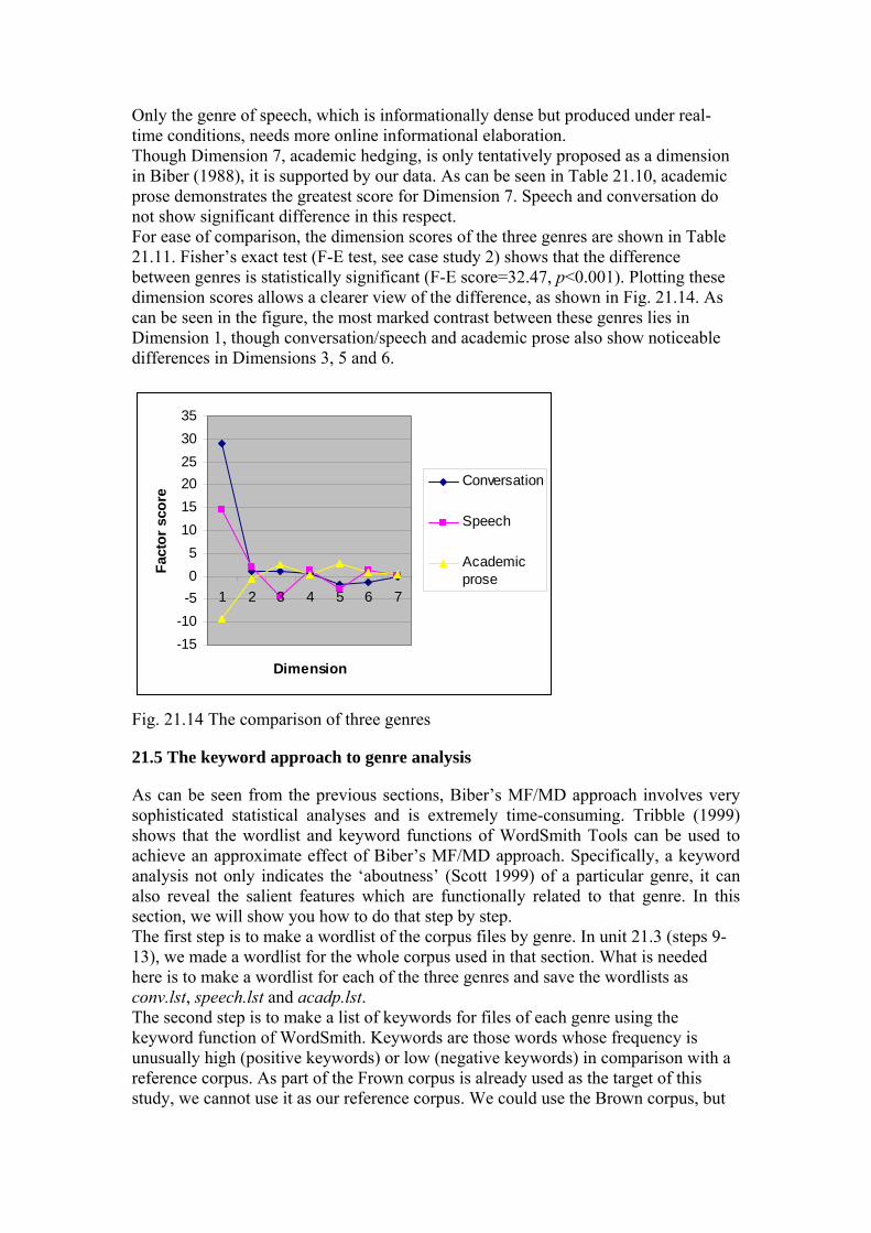
Only the genre of speech, which is informationally dense but produced under real-time conditions, needs more online informational elaboration. Though Dimension 7, academic hedging, is only tentatively proposed as a dimension in Biber (1988), it is supported by our data. As can be seen in Table 21.10, academic prose demonstrates the greatest score for Dimension 7. Speech and conversation do not show significant difference in this respect. For ease of comparison, the dimension scores of the three genres are shown in Table 21.11. Fisher’s exact test (F-E test, see case study 2) shows that the difference between genres is statistically significant (F-E score=32.47, p<0.001). Plotting these dimension scores allows a clearer view of the difference, as shown in Fig. 21.14. As can be seen in the figure, the most marked contrast between these genres lies in Dimension 1, though conversation/speech and academic prose also show noticeable differences in Dimensions 3, 5 and 6.

-15-10-505

101520253035

1 2 3 4 5 6 7

Dimension

Fact

or s

core

Conversation

Speech

Academicprose

Fig. 21.14 The comparison of three genres

21.5 The keyword approach to genre analysis

As can be seen from the previous sections, Biber’s MF/MD approach involves very sophisticated statistical analyses and is extremely time-consuming. Tribble (1999) shows that the wordlist and keyword functions of WordSmith Tools can be used to achieve an approximate effect of Biber’s MF/MD approach. Specifically, a keyword analysis not only indicates the ‘aboutness’ (Scott 1999) of a particular genre, it can also reveal the salient features which are functionally related to that genre. In this section, we will show you how to do that step by step. The first step is to make a wordlist of the corpus files by genre. In unit 21.3 (steps 9-13), we made a wordlist for the whole corpus used in that section. What is needed here is to make a wordlist for each of the three genres and save the wordlists as conv.lst, speech.lst and acadp.lst. The second step is to make a list of keywords for files of each genre using the keyword function of WordSmith. Keywords are those words whose frequency is unusually high (positive keywords) or low (negative keywords) in comparison with a reference corpus. As part of the Frown corpus is already used as the target of this study, we cannot use it as our reference corpus. We could use the Brown corpus, but

that corpus sampled texts in the early 1960s, well before the data used in this study. Consequently we decide to use a corpus of British English as a reference. It is far from ideal to use a British English corpus to provide a reference wordlist for American English data. Using a British English corpus may give prominence to Americanisms in our data. However, given that the three genres will be compared against the same reference corpus, using British English as a reference will not affect our observations notably if the assumption holds that the genres studied here use Americanisms with roughly similar frequency. One further issue related to the reference corpus is that it is clearly much larger than the corpora that are contrasted with it. Tribble (1999:171) claims that the size of the corpus from which the reference wordlist is created is relatively unimportant. Before we undertake a keyword analysis, we will first carry out a baseline test to verify this claim by comparing the keyword lists of the two spoken genres, which were created using a reference wordlist from the one-million-word FLOB corpus and a reference wordlist from the 100-million-word BNC corpus. Both of the reference wordlists are available on our companion website. We assume that you have downloaded and saved them as flob.lst and bnc.lst. It is important to note that keywords are extracted from our American data while FLOB or the BNC only act as a reference corpus. To make a keyword list for the genre of conversation using flob.lst, do the following:

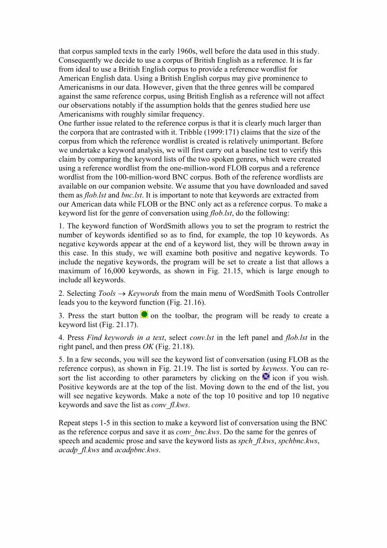
1. The keyword function of WordSmith allows you to set the program to restrict the number of keywords identified so as to find, for example, the top 10 keywords. As negative keywords appear at the end of a keyword list, they will be thrown away in this case. In this study, we will examine both positive and negative keywords. To include the negative keywords, the program will be set to create a list that allows a maximum of 16,000 keywords, as shown in Fig. 21.15, which is large enough to include all keywords.

2. Selecting Tools → Keywords from the main menu of WordSmith Tools Controller leads you to the keyword function (Fig. 21.16).

3. Press the start button on the toolbar, the program will be ready to create a keyword list (Fig. 21.17).

4. Press Find keywords in a text, select conv.lst in the left panel and flob.lst in the right panel, and then press OK (Fig. 21.18).

5. In a few seconds, you will see the keyword list of conversation (using FLOB as the reference corpus), as shown in Fig. 21.19. The list is sorted by keyness. You can re-sort the list according to other parameters by clicking on the icon if you wish. Positive keywords are at the top of the list. Moving down to the end of the list, you will see negative keywords. Make a note of the top 10 positive and top 10 negative keywords and save the list as conv_fl.kws. Repeat steps 1-5 in this section to make a keyword list of conversation using the BNC as the reference corpus and save it as conv_bnc.kws. Do the same for the genres of speech and academic prose and save the keyword lists as spch_fl.kws, spchbnc.kws, acadp_fl.kws and acadpbnc.kws.

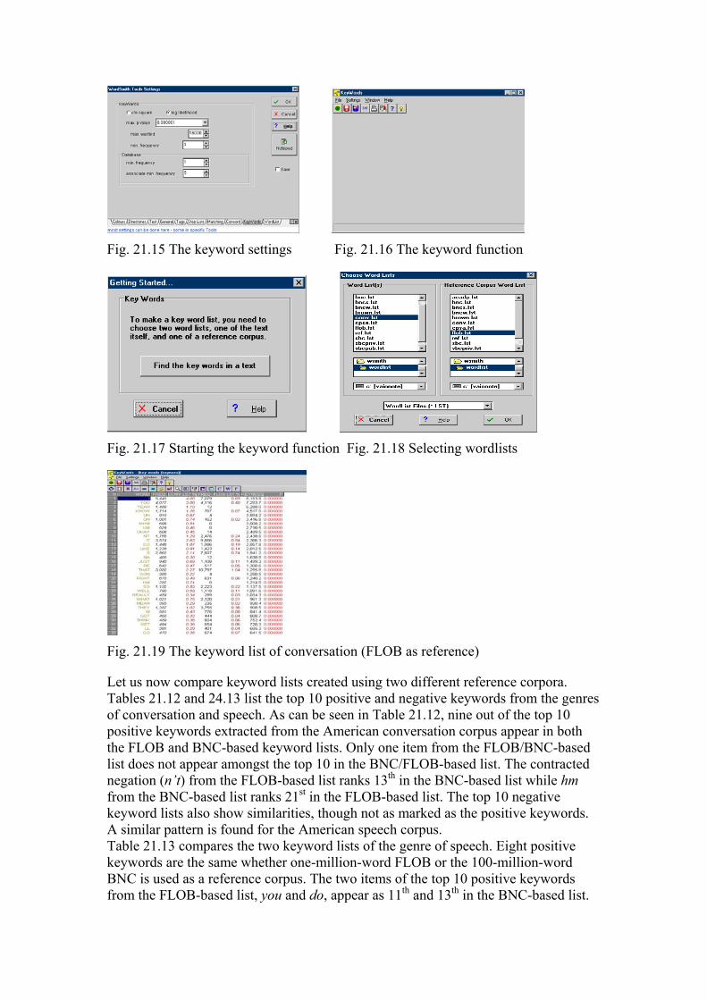
Fig. 21.15 The keyword settings Fig. 21.16 The keyword function

Fig. 21.17 Starting the keyword function Fig. 21.18 Selecting wordlists

Fig. 21.19 The keyword list of conversation (FLOB as reference)

Let us now compare keyword lists created using two different reference corpora. Tables 21.12 and 24.13 list the top 10 positive and negative keywords from the genres of conversation and speech. As can be seen in Table 21.12, nine out of the top 10 positive keywords extracted from the American conversation corpus appear in both the FLOB and BNC-based keyword lists. Only one item from the FLOB/BNC-based list does not appear amongst the top 10 in the BNC/FLOB-based list. The contracted negation (n’t) from the FLOB-based list ranks 13th in the BNC-based list while hm from the BNC-based list ranks 21st in the FLOB-based list. The top 10 negative keyword lists also show similarities, though not as marked as the positive keywords. A similar pattern is found for the American speech corpus. Table 21.13 compares the two keyword lists of the genre of speech. Eight positive keywords are the same whether one-million-word FLOB or the 100-million-word BNC is used as a reference corpus. The two items of the top 10 positive keywords from the FLOB-based list, you and do, appear as 11th and 13th in the BNC-based list.

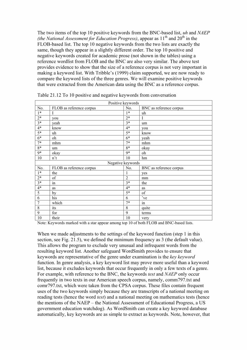
The two items of the top 10 positive keywords from the BNC-based list, uh and NAEP (the National Assessment for Education Progress), appear as 11th and 20th in the FLOB-based list. The top 10 negative keywords from the two lists are exactly the same, though they appear in a slightly different order. The top 10 positive and negative keywords created for academic prose (not shown in the tables) using a reference wordlist from FLOB and the BNC are also very similar. The above test provides evidence to show that the size of a reference corpus is not very important in making a keyword list. With Tribble’s (1999) claim supported, we are now ready to compare the keyword lists of the three genres. We will examine positive keywords that were extracted from the American data using the BNC as a reference corpus.

Table 21.12 To 10 positive and negative keywords from conversation Positive keywords

No. FLOB as reference corpus No. BNC as reference corpus 1* I 1* uh 2* you 2* I 3* yeah 3* um 4* know 4* you 5* uh 5* know 6* oh 6* yeah 7* mhm 7* mhm 8* um 8* okay 9* okay 9* oh 10 n’t 10 hm

Negative keywords No. FLOB as reference corpus No. BNC as reference corpus 1* the 1 yes 2* of 2 mm 3* in 3* the 4* as 4* as 5 by 5* of 6 his 6 ’ve 7 which 7* in 8 its 8 quite 9 for 9 terms 10 their 10 very Note: Keywords marked with a star appear among top 10 of both FLOB and BNC-based lists. When we made adjustments to the settings of the keyword function (step 1 in this section, see Fig. 21.5), we defined the minimum frequency as 3 (the default value). This allows the program to exclude very unusual and infrequent words from the resulting keyword list. Another safeguard WordSmith provides to ensure that keywords are representative of the genre under examination is the key keyword function. In genre analysis, a key keyword list may prove more useful than a keyword list, because it excludes keywords that occur frequently in only a few texts of a genre. For example, with reference to the BNC, the keywords test and NAEP only occur frequently in two texts in our American speech corpus, namely, comm797.txt and comr797.txt, which were taken from the CPSA corpus. These files contain frequent uses of the two keywords simply because they are transcripts of a national meeting on reading tests (hence the word test) and a national meeting on mathematics tests (hence the mentions of the NAEP – the National Assessment of Educational Progress, a US government education watchdog). As WordSmith can create a key keyword database automatically, key keywords are as simple to extract as keywords. Note, however, that

as negative keywords are omitted automatically from a key keyword list, we will compare negative keywords from the keyword lists rather than key keyword lists.

Table 21.13 To 10 positive and negative keywords from speech Positive keywords

No. FLOB as reference corpus No. BNC as reference corpus 1* we 1* we 2* I 2* that 3* that 3 uh 4 you 4* I 5* think 5* test 6* ’re 6* think 7* okay 7 NAEP 8* what 8* okay 9* test 9* ’re 10 do 10* what

Negative keywords No. FLOB as reference corpus No. BNC as reference corpus 1* his 1* the 2* the 2* his 3* he 3* her 4* her 4* by 5* of 5* he 6* by 6* of 7* she 7* she 8* had 8* had 9* was 9* its 10* its 10* was To make a key keyword list of the conversation genre, do the following:

1. If you have not yet done so, adjust WordSmith settings to ignore CLAWS POS tags (steps 9-10 in unit 21.3).

2. Load the 31 files of the conversation genre. Select Tools → Wordlist from the menu of WordSmith Tools Controller. Press the Start button and select Make a batch now (see Fig. 21.12 in unit 21.3).

3. A dialogue box will appear that allows you to specify the directory and filenames for the resulting wordlists. Select use mask, type in conv (the typing space allows up to four characters), and press OK as shown in Fig. 21.20.

4. As the program progresses, a window shows that the resulting wordlists are named conv0001.lst…conv0031.lst and saved in the directory c:\wsmith\wordlist (Fig. 21.21). Press OK.

5. Select Tools → Keywords from the menu of WordSmith Tools Controller (see Fig. 21.16 earlier in this section).

6. Select File → New Database from the menu (Fig. 21.22).

7. Select conv0001.lst…conv0031.lst from the left panel and bnc.lst from the right panel. Press OK (Fig. 21.23).

8. In the dialogue box, specify the directory for the database of key keywords, select use mask and type in conv, and then press OK (Fig. 21.24).

Fig. 21.20 Making a batch of wordlists Fig. 21.21 The result of the batch command

Fig. 21.22 Creating a key keyword list Fig.21.23 Selecting wordlists and reference list

Fig. 21.24 Making a key keyword list Fig. 21.25 The resulting key keyword list

9. You will see a window showing that a new database of key keywords has been created and saved as conv0001.kdb in the directory of c:\wsmith\keywords. Press OK as shown in Fig. 21.25.

10. To view the key keyword list, select File → Open Database from the menu (see Fig. 21.22 above), select conv0001.kdb, and press OK. Table 21.14 lists the top 10 key keywords from conversation and speech. It also shows as a percentage the frequency of the keyword in terms of how often it occurs in the genre (you can find this data by opening the relevant wordlist, pressing the function key F12 on your keyboard or clicking on in the toolbar, and typing a search word) as well as the coverage of the keywords. As can be seen from the table, over 50% of the texts in each genre contain these keywords.

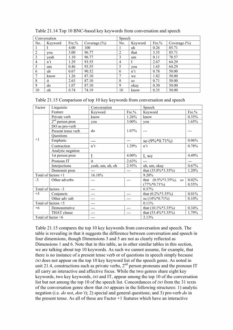
Table 21.14 Top 10 BNC-based key keywords from conversation and speech Conversation Speech No. Keyword Fre.% Coverage (%) No. Keyword Fre.% Coverage (%) 1 I 4.00 100 1 uh 0.26 85.71 2 you 3.00 96.77 2 that 3.35 85.71 3 yeah 1.10 96.77 3 um 0.11 78.57 4 n’t 1.29 93.55 4 I 2.67 64.29 5 um 0.46 93.55 5 you 1.65 64.29 6 uh 0.67 90.32 6 n’t 0.78 50.00 7 know 1.26 87.10 7 we 1.82 50.00 8 it 2.63 87.10 8 so 0.71 50.00 9 do 1.07 87.10 9 okay 0.30 50.00 10 oh 0.74 74.19 10 know 0.35 50.00

Table 21.15 Comparison of top 10 key keywords from conversation and speech Conversation Speech Factor Linguistic

Feature Keyword Fre.% Keyword Fre.% Private verb know 1.26% know 0.35% 2nd person pron you 3.00% you 1.65% DO as pro-verb Present tense verb Questions

do

1.07%

---

---

Emphatic --- --- so (9%*0.71%) 0.06% Contraction Analytic negation

n’t 1.29% n’t 0.78%

1st person pron I 4.00% I, we 4.49% Pronoun IT it 2.63% --- --- Interjections yeah, um, uh, oh 2.93% uh, um, okay 0.67%

+1

Demonstr pron --- --- that (35.8%*3.35%) 1.20% Total of factors +1 16.18% 9.20% -3 Other adverbs --- --- that (0.5%*3.35%), so

(77%*0.71%) 0.02% 0.55%

Total of factors –3 --- 0.57% Conjuncts --- --- that (0.2%*3.35%) 0.01% +5 Other adv sub --- --- so (14%*0.71%) 0.10%

Total of factors +5 --- 0.11% Demonstrative --- --- that (10.1%*3.35%) 0.34% +6 THAT clause --- --- that (53.4%*3.35%) 1.79%

Total of factor +6 --- 2.13% Table 21.15 compares the top 10 key keywords from conversation and speech. The table is revealing in that it suggests the difference between conversation and speech in four dimensions, though Dimensions 3 and 5 are not as clearly reflected as Dimensions 1 and 6. Note that in this table, as in other similar tables in this section, we are talking about top 10 keywords. As such we cannot assume, for example, that there is no instance of a present tense verb or of questions in speech simply because DO does not appear on the top 10 key keyword list of the speech genre. As noted in unit 21.4, constructions such as private verbs, 2nd person pronouns and the pronoun IT all carry an interactive and affective focus. While the two genres share eight key keywords, two key keywords, DO and IT, appear among the top 10 of the conversation list but not among the top 10 of the speech list. Concordances of DO from the 31 texts of the conversation genre show that DO appears in the following structures: 1) analytic negation (i.e. do not, don’t); 2) special and general questions; and 3) pro-verb do in the present tense. As all of these are Factor +1 features which have an interactive

focus, we will not make a distinction between them; rather the gross percentage will be used for all of these features. Similarly, n’t is both a contraction and an analytic negation, so we will not draw a distinction between the two. Another feature of note in Table 21.15 is interjections. Interjections are of note for two reasons. Firstly, they are more common in conversation than speech. Secondly, interjections were not considered as discourse markers by Biber (1988), though they are actually used in the same way as discourse particles to maintain conversational coherence (Schiffrin 1982) and are typical of spoken language (see Aijmer 1987: 61-86 for an interesting account of the functions of oh and ah in the London-Lund corpus). Hence, while interjections are not included as a relevant linguistic feature in the MF/MD approach, they are an important feature in a keyword analysis. Two key keywords that are found among the top 10 of the speech list but not among the top 10 of the conversation list are THAT and SO. As CLAWS makes a distinction between the different uses of these words, it is easy to determine their proportions. Concordances of that_* from the 14 texts of the speech genre show that THAT is used in following contexts: 1) THAT-clause (that_CS*): 53.4%. We will not differentiate between the three types of THAT clauses because they are all features with positive weights on Factor 6; 2) demonstrative pronoun (that_DD1 context 0L 2R = ~*_NN*): 35.8%; 3) demonstrative (that_DD1 context 0L 2R = *_NN*): 10.1%; 4) emphatic (that_RG): 0.5%; and 5) other adverbial subordination (that_REX21): 0.2%. The keyword SO is used in the following contexts: 1) other adverbs (so_RR*): 77%; 2) other adverbial subordination (so_CS*): 14%; and 3) emphatics (so_RG*): 9%. The overall percentages of the two keywords are allocated to appropriate features accordingly. It can be seen in Table 21.15 that the total of Factor +1 for the conversation genre (16.18%) is considerably greater than the total for the speech genre 9.20%. Conversely, in relation to Factors +3 and +5, the total of Factor +6 for the speech genre is significantly greater than that for conversation, suggesting a possibly significant difference between the two spoken genres along Dimension 6, which indicates the level of online elaboration. These observations of the two spoken genres are in line with the MF/MD results in unit 21.4. In contrast, the top 10 key keywords from the genre of academic prose include: of, the, is, formula, system, American, B, G, C and program. The first two key keywords are of and the. Of as a preposition adds a negative weight to the dimension of informational vs. involved production. Tribble (1999: 175-177) observes that of and the are typically associated with nouns. In academic prose, for example, of is typically used as a post-modifier in the N1 + of + N2 structure (e.g. center of mass, clusters of galaxies). The definite article the is also associated with nouns. In an MD/MF analysis, nouns of the nominalization type are a feature with a positive loading for Dimension 3 (explicit vs. situation-dependent reference) while nouns of other types are a feature with a negative loading for Dimension 1 (informational vs. involved focus). Is as a main verb is typically used in academic prose to make a statement or claim (e.g. it is an excellent example of…, it is the user’s responsibility to…). The four content words (formula, system, American and program) indicate the ‘aboutness’ of academic prose. The three letters are used mainly as part of a list or variable labels, which are typical of academic prose. These key keywords enable us to get a general view of the content and style of academic prose.

Table 21.16 Top 10 FLOB-based negative keywords of three genres Factor Linguistic feature Conversation Speech Academic prose 2nd person pronouns --- --- you

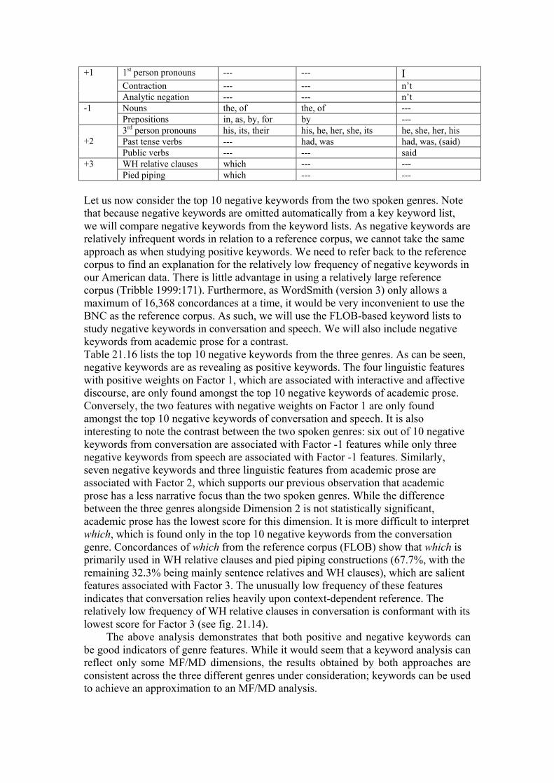
1st person pronouns --- --- I Contraction --- --- n’t

+1

Analytic negation --- --- n’t Nouns the, of the, of --- -1 Prepositions in, as, by, for by --- 3rd person pronouns his, its, their his, he, her, she, its he, she, her, his Past tense verbs --- had, was had, was, (said)

+2

Public verbs --- --- said WH relative clauses which --- --- +3 Pied piping which --- ---

Let us now consider the top 10 negative keywords from the two spoken genres. Note that because negative keywords are omitted automatically from a key keyword list, we will compare negative keywords from the keyword lists. As negative keywords are relatively infrequent words in relation to a reference corpus, we cannot take the same approach as when studying positive keywords. We need to refer back to the reference corpus to find an explanation for the relatively low frequency of negative keywords in our American data. There is little advantage in using a relatively large reference corpus (Tribble 1999:171). Furthermore, as WordSmith (version 3) only allows a maximum of 16,368 concordances at a time, it would be very inconvenient to use the BNC as the reference corpus. As such, we will use the FLOB-based keyword lists to study negative keywords in conversation and speech. We will also include negative keywords from academic prose for a contrast. Table 21.16 lists the top 10 negative keywords from the three genres. As can be seen, negative keywords are as revealing as positive keywords. The four linguistic features with positive weights on Factor 1, which are associated with interactive and affective discourse, are only found amongst the top 10 negative keywords of academic prose. Conversely, the two features with negative weights on Factor 1 are only found amongst the top 10 negative keywords of conversation and speech. It is also interesting to note the contrast between the two spoken genres: six out of 10 negative keywords from conversation are associated with Factor -1 features while only three negative keywords from speech are associated with Factor -1 features. Similarly, seven negative keywords and three linguistic features from academic prose are associated with Factor 2, which supports our previous observation that academic prose has a less narrative focus than the two spoken genres. While the difference between the three genres alongside Dimension 2 is not statistically significant, academic prose has the lowest score for this dimension. It is more difficult to interpret which, which is found only in the top 10 negative keywords from the conversation genre. Concordances of which from the reference corpus (FLOB) show that which is primarily used in WH relative clauses and pied piping constructions (67.7%, with the remaining 32.3% being mainly sentence relatives and WH clauses), which are salient features associated with Factor 3. The unusually low frequency of these features indicates that conversation relies heavily upon context-dependent reference. The relatively low frequency of WH relative clauses in conversation is conformant with its lowest score for Factor 3 (see fig. 21.14).

The above analysis demonstrates that both positive and negative keywords can be good indicators of genre features. While it would seem that a keyword analysis can reflect only some MF/MD dimensions, the results obtained by both approaches are consistent across the three different genres under consideration; keywords can be used to achieve an approximation to an MF/MD analysis.

21.6 Unit summary and suggestions for further study

In this unit, we compared the genres of conversation and speech in American English alongside seven dimensions, using Biber’s MF/MD approach and Tribble’s keyword approach using wordSmith. The results obtained by the two approaches are similar. The most significant difference between conversation and speech lies in Dimension 1, a measure of the informational vs. involved distinction. They also differ marginally alongside Dimension 6, which indicates the level of online elaboration. This means that conversation is considerably more interactive and affective than speech. While speech is informationally dense, it is subject to real-time production conditions and thus speech needs online informational elaboration. The two spoken genres differ significantly from academic prose along Dimensions 1, 3, and 5. This means that on the one hand, academic prose is the most ‘literate’, technical, and abstract of the three genres under consideration while on the other hand, this written genre tends to make explicit in-text reference whereas the two spoken genres make context-dependent references. Methodologically, the MF/MD approach, while providing a powerful and comprehensive tool for genre analysis, requires considerable expertise in data extraction and statistical analysis. The keyword approach, in contrast, provides a less demanding approach to genre analysis. But since this approach provides a less comprehensive contrast of genres and may not work for some fine-grained types of genre analysis, it is not simply a substitute for MF/MD analysis. Nevertheless, as the keyword approach requires little technical expertise and can be undertaken swiftly, it provides a quick and simple means of evaluating a genre against Biber’s dimensions. The keyword approach to genre analysis provides linguists with a powerful and easily used tool. Biber (1987) compared nine written genres from British and American English, and Biber (1988) compared 21 genres in British English. In this unit we were concerned with conversation and speech in American English. This unit might motivate you to pursue genre analysis from a diachronic viewpoint by comparing genres in the LOB and FLOB corpora. Alternatively, you might wish to compare the five types of imaginative texts (text categories K, L, M, N and P) in the Brown corpus to see whether its sampling frame (see unit 7.4), which has, to date, rarely been questioned, is justified.