UNIT 3 LAMINAR AND TURBULENT FLOW Orifice · 2016-09-12 · Mathematically coefficient of contraction, The value of Coefficient of contraction varies slightly with the available head

SME 1202 Fluid Mechanics and Machinery Unit-3 LAMINAR AND TURBULENT FLOW Prepared by: Mr.S.Senthilkumar

Page 1 of 30

UNIT 3 LAMINAR AND TURBULENT FLOW

Orifice

Orifice is a small opening on the side or at the bottom of a tank, through which a fluid is flowing.

The orifices are classified according to the size, shape, nature of discharge and shape of the edge.

1. According to the size of orifice and head of liquid from the centre of the orifice: Small orifice

and Large orifice.

Small Orifice: If the head of liquid from the centre of orifice is more than five times the depth of

orifice, the orifice is called small orifice.

Large Orifice: If the head of liquid is less than five times the depth of orifice, it is known as large

orifice.

2. According to shape of orifice: (i) Circular orifice, (ii) Triangular orifice,( iii) Rectangular orifice

and (iv) Square orifice

3. According to their cross-sectional area or edge: (i) Sharp-edged orifice and (ii) Bell mouthed

orifice

4. According to the discharge condition: (i) Free discharging orifices (ii) Fully drowned or

submerged orifices and (iii) Partially submerged orifices.

Flow through a Small Orifice

Flow from a tank through a hole in the side.

The edges of the hole are sharp to minimize frictional losses by minimizing the contact between the hole

and the liquid. The streamlines at the orifice contract reducing the area of flow. This contraction is

called the vena contracta.

The amount of contraction must be known to calculate the flow.

Applying Bernoulli’s equation along the streamline joining point 1 on the surface to point 2 at the centre

of the orifice.

At the surface velocity is negligible (v1 = 0) and the pressure atmospheric (p1 = 0). At the orifice the jet

is open to the atmosphere so again the pressure is atmospheric (p2 = 0).

If we take the datum line through the orifice then z1 = H and z2 =0, leaving h = 𝑣2

2

2𝑔

𝑣2 = 𝑣𝑡ℎ = √2𝑔𝐻

This theoretical value of velocity is an overestimate as friction losses have not been taken into account.

A coefficient of velocity is used to correct the theoretical velocity,

𝑣𝑎 = 𝐶𝑉 × 𝑣𝑡ℎ Each orifice has its own coefficient of velocity, they usually lie in the range 0.97 - 0.99

The discharge through the orifice = jet area X jet velocity

The area of the jet is the area of the vena contracta and not the area of the orifice.

We use a Coefficient of contraction to get the area of the jet,Aa.

Aa = Cc X area of orifice


Page 2 of 30

Discharge through the orifice;

Q = Av

Actual discharge, Qa = Cd X Qth

Qth = Area of orifice X vth

Hydraulic Coefficients

The following three coefficients are known as hydraulic coefficients or orifice coefficients.

Coefficient of contraction

Coefficient of velocity

Coefficient of discharge

Coefficient Of Contraction

The ratio of the area of the jet, at vena-contracta, to the area of the orifice is known as coefficient of

contraction. Mathematically coefficient of contraction,

The value of Coefficient of contraction varies slightly with the available head of the liquid, size and

shape of the orifice. The average value of is 0.64.

Coefficient of Velocity

The ratio of actual velocity of the jet, at vena-contracta, to the theoretical velocity is known

as coefficient of velocity.

The theoretical velocity of jet at vena-contracta is given by the relation, 𝑣𝑡ℎ = √2𝑔𝐻, where H is the

head of water at vena-contracta. Mathematically coefficient of velocity,

The difference between the velocities is due to friction of the orifice. The value of Coefficient of

velocity varies slightly with the different shapes of the edges of the orifice. This value is very small for

sharp-edged orifices. For a sharp edged orifice, the value of 𝐶𝑣 increases with the head of water.

Coefficient of Discharge

The ratio of a actual discharge through an orifice to the theoretical discharge is known as coefficient of

discharge. Mathematically coefficient of discharge,


Page 3 of 30

Thus the value of coefficient of discharge varies with the values of 𝐶𝐶 and 𝐶𝑣 . An average of

coefficient of discharge varies from 0.60 to 0.64.

Determination of Coefficient of Discharge (Cd)

The water is allowed to flow through an orifice provided in a tank under a constant head H. The water is

collected in a collecting tank for a known height. The time of collection of water in the collecting tank

is noted down.

Then

actual discharge through orifice, Qa = Area of collecting tank(A) x Height of water(h)

𝑡𝑖𝑚𝑒 (𝑡)

and theoretical discharge, 𝑄𝑡ℎ = area of orifice x √2𝑔𝐻

𝐶𝑑 =𝑄𝑎

𝑄𝑡ℎ

Determination of Coefficient of Velocity(Cv)

In the jet issuing from an orifice under a constant head of H, let the coordinate distances be ‘x’

horizontally and ‘y’ vertically of a water particle be traced in ‘t’ seconds from vena contracta.

Actual velocity, va = √𝑔𝑥2

2𝑦⁄ and theoretical velocity, 𝑣𝑡ℎ=√2𝑔𝐻

Coefficient of Velocity, Cv = √

𝑔𝑥2

2𝑦

√2𝑔𝐻 = √

𝑥2

4𝑦𝐻

𝐶𝑣 = √𝑥2

4𝑦𝐻

Discharge Through a Large Rectangular Orifice

Consider a large rectangular orifice of width ‘b’ provided on a vertical side of a tank, with a constant

head ‘H’ above its centre, discharging freely in to atmosphere.


Page 4 of 30

Let, H1 = head of water above bottom edge of the orifice and H2 = head of water above the top edge of

orifice. Therefore, the height of orifice is (H1-H2).

Cd= co-efficient of discharge.

Consider a thin horizontal strip of depth 'dh' and ‘h’ be the head of water above the strip.

Area of the strip = b dh; theoretical velocity of water through the strip = √2𝑔ℎ

Discharge through elementary strip = b dh √2𝑔ℎ

Total discharge through the entire orifice =𝐶𝑑 ∫ 𝑏 𝑑ℎ𝐻1

𝐻2√2𝑔ℎ

𝑄𝑎= 𝐶𝑑𝑏√2𝑔 ∫ 𝑑ℎ𝐻1

𝐻2 ℎ½

= 𝐶𝑑𝑏√2𝑔 [ℎ

32⁄

23⁄

]𝐻2

𝐻1

𝑄𝑎 =2

3𝐶𝑑𝑏√2𝑔 [𝐻1

3

2 − 𝐻2

3

2] 𝑚3

𝑠⁄

Discharge through Fully Submerged Orifice

If the discharge side of a large rectangular orifice is under water, then it is known to be fully submerged

or drowned Orifice.

Let, ‘b’ is the width of orifice;

H1 = head of water above bottom edge of the orifice and H2 = head of water above the top edge of

orifice.

Therefore, the height of orifice is (H1-H2)

Head difference between the upstream and downstream side water levels which is responsible for the

flow = H metres.

Cd= co-efficient of discharge.

Discharge, Qa = 𝐶𝑑 × 𝑎𝑟𝑒𝑎 × 𝑣𝑒𝑙𝑜𝑐𝑖𝑡𝑦 = 𝐶𝑑 𝑏(𝐻1 − 𝐻2)√2𝑔𝐻

Discharge through Partially Submerged Orifice

If part of the discharge end of the rectangular orifice is submerged under water, it is known as partially

submerged orifice and the discharge is through two parts.

Upper part is a free orifice and lower part is submerged orifice.


Page 5 of 30

Let, ‘b’ is the width of orifice;

H1 = head of water above bottom edge of the orifice and H2 = head of water above

the top edge of orifice.

Head difference between the upstream and downstream side water levels which is

responsible for the flow = H metres.

Total discharge partially submerged orifice, Q = Q1+Q2

Q1= Discharge through the submerged orifice part

Q2= Discharge through the free orifice part

Q1 = 𝐶𝑑 𝑏(𝐻1 − 𝐻)√2𝑔𝐻

Q2 = 2

3𝐶𝑑𝑏√2𝑔 [𝐻

3

2 − 𝐻2

3

2]

Q = 𝐶𝑑 𝑏(𝐻1 − 𝐻)√2𝑔𝐻 + 2


3

2 − 𝐻2

3

2] 𝑚3

𝑠⁄

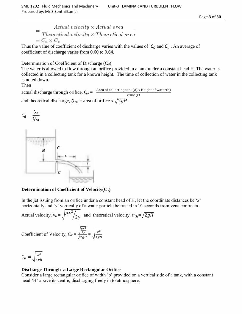
1. The head of water over an orifice of diameter 50 mm is 12 m. Find the actual discharge and actual

velocity of jet at vena contracta. Take Cd = 0.6 and Cv = 0.98.

Solution: Diameter of orifice, d = 50 mm = 0.05 m

Head, H=12 m

Cd = 0.6 and Cv = 0.98

Theoretical velocity, vth = √2𝑔𝐻 = √2 × 9.81 × 12 = 15.34 m/s

Actual velocity, va = Cv × vth = 0.98 × 15.34 = 15.03 m/s

Actual discharge, Qa = Cd× Qth = Cd a √2𝑔𝐻 = 0.6 × 𝜋

4× 𝑑2 × 15.34 = 0.6×

𝜋

4× 0.052 × 15.34

= 0.01807 𝑚3

𝑠⁄

2. The head of water over the centre of an orifice of diameter 30 mm is 1.5 m. The actual discharge

through the orifice is 2.35 litres/sec. Find the co-efficient of discharge.

Actual discharge, Qa = 2.35 lit/s = 0.00235𝑚3

𝑠⁄

Theoretical discharge, Qth = a √2𝑔𝐻 = 𝜋

4× 𝑑2 × √2𝑔𝐻

Qth= 𝜋

4× 0.032 × √2 × 9.81 × 1.5 = 0.003835 𝑚3

𝑠⁄

Co-efficient of discharge, Cd = 𝑄𝑎

𝑄𝑡ℎ = 0.00235/0.003835 = 0.613

3. A jet of water, issuing from a sharp edged vertical orifice under a constant head of 60 cm, has the

horizontal and vertical co-ordinates measured from the vena contracta at a certain point as 10 cm and

0.45 cm respectively. Find the value of Cv. Also find the value of Cc if Cd = 0.6

Solution:

Cv = √𝑥2

4𝑦𝐻 = √

0.12

4×0.0045×0.6 = 0.96

We know that, Cd= Cc x Cv

Cc= Cd / Cv = 0.6 /0.96 = 0.625


Page 6 of 30

4. The head of water over an orifice of diameter 100 mm is 5 m. The water coming out from orifice is

collected in a circular tank of diameter 2 m. The rise of water level in circular lank is 0.45 m in 30

seconds. Also the coordinates of a certain point on the jet, measured from vena contracta are 100 cm

horizontal and 5.2 cm vertical. Find the hydraulic co-efficients.

Solution:

Actual discharge, Qa= Area of collecting tank x height of collection/time

= 𝜋𝐷2

4 × ℎ/𝑡 =

𝜋

4× 22 × 0.45/30 = 0.047124 m3/s

Theoretical discharge, Qth = a √2𝑔𝐻 = 𝜋

4× 𝑑2 × √2𝑔𝐻

Qth= 𝜋

4× 0.12 × √2 × 9.81 × 5 = 0.0778 𝑚3

𝑠⁄

Co-efficient of discharge, Cd = 𝑄𝑎

𝑄𝑡ℎ = 0.047124/0.0778 = 0.61

Cv = √𝑥2

4𝑦𝐻 = √

12

4×0.052×5 = 0.98

Cc = Cd/Cv = 0.61/0.98 = 0.62

5. A rectangular orifice, 2 m wide and 1.5 m deep is discharging water from a tank. If the water level in

the tank is 3 m above the top edge of the orifice, find the discharge through the orifice. Take Cd =

0.6.

H1 = head of water above bottom edge of the orifice = 1.5 + 3 = 4.5 m

H2 = head of water above the top edge of orifice = 3 m

Discharge through the free orifice, 𝑄𝑎 =2

3𝐶𝑑𝑏√2𝑔 [𝐻1

3

2 − 𝐻2

3

2] 𝑚3

𝑠⁄

=2

3 × 𝐶𝑑 × 𝑏 × √2𝑔 × [𝐻1

3

2 − 𝐻2

3

2] 𝑚3

𝑠⁄

= 2

3 × 0.6 × 2 × √2 × 9.81 × [4.5

3

2 − 33

2] = 15.414 m3/s

6. Find the discharge through a fully submerged orifice of width 2 m if the difference of water

levels on both the sides of the orifice be 800 mm. The height of water from top and bottom of the

orifice are 2.5 m and 3 m respectively. Take Cd = 0.62.

Discharge, Qa = 𝐶𝑑 𝑏(𝐻1 − 𝐻2)√2𝑔𝐻 = 0.62 x 2 x (3 - 2.5) x √2 × 9.81 × 0.8 = 2.46 m3/s

7. A rectangular orifice of 1.5 m wide and 1.2 m deep is provided in one side of a large lank. The

water level on one side of the orifice is 2 m above the top edge of the orifice, while on the other

side of the orifice the water level is 0.4 m below its top edge. Calculate the discharge through the

orifice if Cd= 0.62

Solution:

H1 = head of water above bottom edge of the orifice = 1.2 + 2 = 3.2 m

H2 = head of water above the top edge of orifice = 2 m

H = Head difference = 2 + 0.4 = 2.4 m

Total discharge partially submerged orifice, Q = Q1+Q2

Q1= Discharge through the submerged orifice part


Page 7 of 30

Q2= Discharge through the free orifice part

Q = 𝐶𝑑 𝑏(𝐻1 − 𝐻)√2𝑔𝐻 + 2


3

2 − 𝐻2

3

2] 𝑚3

𝑠⁄

= 0.62 x 1.5 x (3.2 – 2.4) x √2 × 9.81 × 2.4 + 2

3× 0.62 × 1.5 × √2 × 9.81 × [2.4

3

2 − 23

2]

= 5.1054 + 2.4432 = 7.5486 m3/s

Flow Over Notches and Weirs

A notch is a device used for measuring the rate of flow of a liquid through a small channel.

A weir is a concrete or masonry structure placed in the open channel over which the flow occurs.

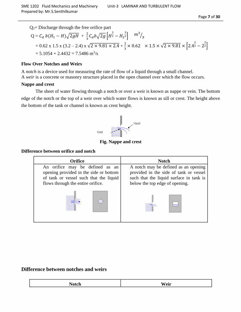
Nappe and crest

The sheet of water flowing through a notch or over a weir is known as nappe or vein. The bottom

edge of the notch or the top of a weir over which water flows is known as sill or crest. The height above

the bottom of the tank or channel is known as crest height.

Fig. Nappe and crest

Difference between orifice and notch

Orifice Notch

An orifice may be defined as an

opening provided in the side or bottom

of tank or vessel such that the liquid

flows through the entire orifice.

A notch may be defined as an opening

provided in the side of tank or vessel

such that the liquid surface in tank is

below the top edge of opening.

Difference between notches and weirs

Notch Weir


Page 8 of 30

A notch may be defined as an opening

provided in the side of tank or vessel such

that the liquid surface in tank is below the

top edge of opening.

A weir may be defined as any regular

obstruction in open stream over which the

flow takes place.

Small structure Large structure

Made of metallic plates. Made of concrete/bricks.

Measure small flow rate. Measure large flow rate.

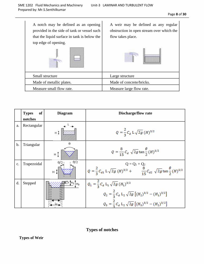
Types of notches

Types of Weir

Types of

notches

Diagram Discharge/flow rate

a. Rectangular

b. Triangular

c. Trapezoidal

Q = Q1 + Q2

d. Stepped

Q = Q1 + Q2 + Q3


Page 9 of 30

1. Shape

Rectangular

Triangular

Trapezoidal

Types of weir on basis of shape

Types of

weir

Diagram Discharge/flow rate

a. Rectangular

b. Triangular

c. Trapezoidal

Q = Q1 + Q2

Note: The discharge equation for rectangular, triangular and trapezoidal weir is same as of notch.

2. Nature of discharge

Free: Liquid level on the downstream side is lower than the crest.

Free flowing weir

Drowned: Liquid level submerges the crest

Drowned weir

3. Width of crest

Sharp: The crest is narrow

Sharp crest weir


Page 10 of 30

Broad: The crest is broad

Broad crest weir

1. Determine flow rate through a rectangular notch if L = 0.20 m and H = 0.15 m. Take value of

cd = 0.645

Solution

= 0.022 m3/s

2. Determine flow rate through a triangular notch if H = 0.20 m and . Take value of cd =

0.85.

Solution

= 0.0207 m3/s

3. Determine flow rate through a rectangular weir if L = 0.30 m and H = 0.25 m. Take value of

cd = 0.95

Solution

= 0.105 m3/s


Page 11 of 30

Flow in pipes

In this chapter, however, a method of expressing the loss using an average flow velocity is stated.

Studies will be made on how to express losses caused by achange in the cross sectional

area of a pipe, a pipe bend and a valve, in addition to the frictional loss of a pipe.Consider a case where

fluid runs from a tank into a pipe whose entrance section isfully rounded. At the entrance, the velocity

distribution is roughly uniform while thepressure head is lower by V2/2g . As shown in below Figure

,the section from theentrance to just where the boundary layer develops to the tube centre is called

theinlet or entrance region, whose length is called the inlet or entrance length.

For steady flow at a known flow rate, these regions exhibit the following:

Laminar flow:A local velocity constant with time, but which varies spatially due

to viscous shear and geometry.

Turbulent flow: A local velocity which has a constant mean value but also has a

statistically random fluctuating component due to turbulence in the flow. Typical

plots of velocity time histories for laminar flow, turbulent flow, and the region of

transition between the two are shown below

Principal parameter used to specify the type of flow regime is the Reynolds number :

V - characteristic flow velocity

D - characteristic flow dimension

μ- dynamic viscosity

υ- kinematic viscosity

We can now define the critical or transition Reynolds number Recr

Re is the Reynolds number below which the flow is laminar, above which the flow

is turbulent While transition can occur over a range of Re, we will use the following for internal

pipe or duct flow:

Major Losses due to pipe Friction Let us study the flow in the region where the velocity distribution is fullydeveloped after passing

through the inlet region as shown below. If a fluid Isflowing in the round pipe of diameter d at the

average flow velocity v, let thepressures at two points distance L apart be p1 and p2 respectively. The

relationshipbetween the velocity u and the loss head h = ( p1 - p2 ) /pg For the laminar flow,the loss head

h is proportional to the flow velocity v while for the turbulent


Page 12 of 30

flow, it turns out to be proportional to v1.75-2 .

The loss head is expressed by the following equation as shown in this equation :

This equation is called the Darcy-Weisbach equation', and the coefficient f is called

the friction coefficient of the pipe.

Minor losses in pipes In a pipe line, in addition to frictional loss, head loss is produced through additional

turbulence arising when fluid flows through such components as change of area change of direction,

branching, junction, bend and valve.

1. Head Loss due to sudden expansion

For a suddenly expanding pipe as shown in below Figure, assume that the pipe ishorizontal, disregard

the frictional loss of the pipe, let h, be the expansion loss, and set up an equation of energy between

sections 1 and 2 as :

2. Head loss at the exit of pipes:

hex = 𝑣2

2𝑔

v = velocity of liquid in the pipe

3. Head loss due to sudden contraction

Owing to the inertia, section 1 (section area A1 )of the fluid shrinks to section 2 (section area Ac)

and then widens to section 3 ( section area A2 ).The loss when the flow is accelerated is

extremely small, followed by ahead loss similar to that in thecase of sudden expansion equation

is expressed by :


Page 13 of 30

hc = 0.5 𝑣2

2

2𝑔

Here Cc = Ac / A2 is a contraction coefficient.

4. Head loss at Inlet of pipe

The loss of head in the case where fluid enters in to a pipe from a large vessel is expressed by

the following equation:

hi = 0.5 𝑣2

2𝑔

5. Head loss due to bend in pipe

hb = k 𝑣2

2𝑔, where k= Coefficient of pipe bend; v = mean velocity of liquid in the pipe.

6. Head loss due to various pipe fittings

hp = k 𝑣2

2𝑔, where k= Coefficient of pipe fittings

7. Head loss due to obstruction

ho = (𝐴

𝐶𝑐(𝐴−𝑎))

2𝑣2

2𝑔

where, A = Are of pipe cross section

a = area of obstruction; v = velocity of liquid

Pipes in series

when pipes of different diameters are connected end to end to form a pipe line, they are said to be in

series. The total loss of energy (or head) will be the sum of the losses in each pipe plus minor losses at

connections.

Example

Consider the two reservoirs shown in figure , connected by a single pipe that changes diameter over its

length. The surfaces of the two reservoirs have a difference in level of 9m. The pipe has a diameter of

200mm for the first 15m (from A to C) then a diameter of 250 mm for the remaining 45m (from C to B)

The join at C is sudden. For both pipes use


Page 14 of 30

f = 0.01.

Total head loss for the system H = height difference of reservoirs

hf1 = head loss for 200mm diameter section of pipe

hf2 = head loss for 250mm diameter section of pipe

hi = head loss at entry point

h j = head loss at join of the two pipes

h ex = head loss at exit point

So

H = hf1 + hf2 + hi + hj + hex = 9m

All losses are, in terms of Q

Substitute these into

hf1 + hf2 + hi + hj + hex = 9m

and solve for Q, to give Q = 0.158 m3/s

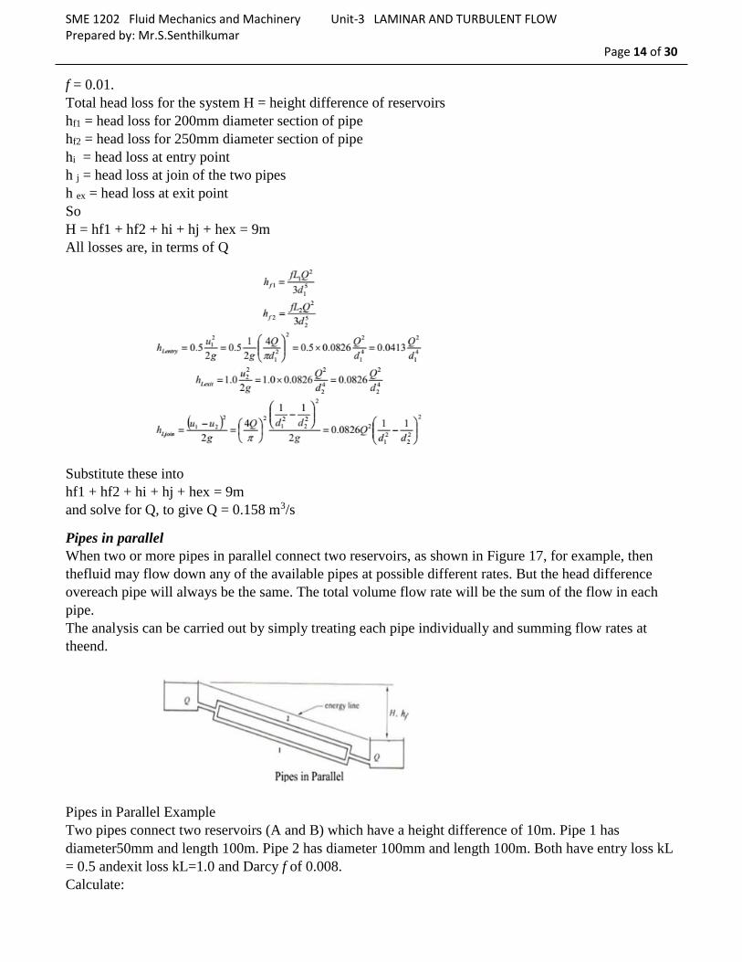
Pipes in parallel

When two or more pipes in parallel connect two reservoirs, as shown in Figure 17, for example, then

thefluid may flow down any of the available pipes at possible different rates. But the head difference

overeach pipe will always be the same. The total volume flow rate will be the sum of the flow in each

pipe.

The analysis can be carried out by simply treating each pipe individually and summing flow rates at

theend.

Pipes in Parallel Example

Two pipes connect two reservoirs (A and B) which have a height difference of 10m. Pipe 1 has

diameter50mm and length 100m. Pipe 2 has diameter 100mm and length 100m. Both have entry loss kL

= 0.5 andexit loss kL=1.0 and Darcy f of 0.008.

Calculate:


Page 15 of 30

a) rate of flow for each pipe

b) the diameter D of a pipe 100m long that could replace the two pipes and provide the same

flow.

using the Darcy equation in terms of Q

And the loss equations in terms of Q:

For pipe 1

For pipe 2

BOUNDARY LAYER FLOWS

Viscous internal flows have the following major boundary layer characteristics:

* An entrance region where the boundary layer grows and dP/dx ≠ constant,

* A fully developed region where:

• The boundary layer fills the entire flow area.

• The velocity profiles, pressure gradient, and w are constant;

i.e. they are not equal to f(x),

• The flow is either laminar or turbulent over the entire length of the flow,

i.e. transition from laminar to turbulent is not considered.

However, viscous flow boundary layer characteristics for external flows are significantly different

as shown below for flow over a flat plate:


Page 16 of 30

Schematic of boundary layer flow over a flat plate

For these conditions, we note the following characteristics:

• The boundary layer thickness grows continuously from the start of the fluid-surface contact, e.g.

the leading edge. It is a function of x, not a constant.

• Velocity profiles and shear stress are f(x,y).

• The flow will generally be laminar starting from x = 0.

• The flow will undergo laminar-to-turbulent transition if the streamwise dimension is greater than a

distance xcr corresponding to the location of the transition Reynolds number Recr.

• Outside of the boundary layer region, free stream conditions exist where velocity gradients and

therefore viscous effects are typically negligible.

As it was for internal flows, the most important fluid flow parameter is the local Reynolds number

defined as

where

ρ = fluid density µ= fluid dynamic viscosity

υ = fluid kinematic viscosity U = characteristic flow velocity

x = characteristic flow dimension

It should be noted at this point that all external flow applications will not use a distance from the

leading edge x as the characteristic flow dimension. For example, for flow over a cylinder, the

diameter will be used as the characteristic dimension for the Reynolds number.

Transition from laminar to turbulent flow typically occurs at the local transition Reynolds number,

which for flat plate flows can be in the range of

500,000 Recr 3,000,00

a

y

x

U•

(x)turbulentlaminar

xcr

laminar toturbulenttransition

edge of boundary layerfree stream

Rex

Ux

Ux


Page 17 of 30

With xcr = the value of x where transition from laminar to turbulent flow occurs, the typical value used

for steady, incompressible flow over a flat plate is

Recr U xcr

500, 000

Thus for flat plate flows for which:

x <xcr the flow is laminar

x ≥ xcr the flow is turbulent

The solution to boundary layer flows is obtained from the reduced “Navier – Stokes” equations, i.e.,

Navier-Stokes equations for which boundary layer assumptions and approximations have been applied.

Flat Plate Boundary Layer Theory

Laminar Flow Analysis

For steady, incompressible flow over a flat plate, the laminar boundary layer equations are:

Conservation of mass:

'X' momentum:

'Y' momentum:

The solution to these equations was obtained in 1908 by Blasius, a student of Prandtl's. He showed that

the solution to the velocity profile, shown in the table below, could be obtained as a function of a single,

non-dimensional variable

defined as

Table: Blasius Velocity Profile

ux

v y

0

u u

x v

u

y

1

d p

d x

1

y u

y

p

y 0


Page 18 of 30

with the resulting ordinary

differential equation:

f 1

2f f 0

and f

u

U

Fluid flow

Fluid flow over bodies frequently occurs in practice and physical phenomena:

Drag force acting on automobile, power lines, trees and underwater pipeline

The lift development by airplane wings

Upward draft of rain, snow and dust particles in high winds

The transportation of red blood cells by blood flow

The vibration and noise generated by bodies moving in a fluid

Power generated by wing turbines and...etc

Drag

The force flowing fluid exerts on a body in the flow direction is called drag.

The drag force can be measured directly by simply attaching the body subjected to fluid

flow to a calibrated spring and measuring the displacement in flow direction (like

measuring weight with a spring scale). Example: using drag-measuring device called drag

balance-using flexible beams fitted with strain gages to measure the drag electronically.

Drag usually an desireble effect, like friction we need to minimize it

Reduction of drag associated with:

Reduction of fuel consumption in automobile, aircraft and submarines

Improved safety and durability of structures subjected to high winds and

Reduction of noise and vibration

Both of pressure force and wall shear force on the surface in the direction of flow is called

drag force.

The components of the pressure and wall shear force in the direction normal to the flow

tend to move body in that direction and its sum is called lift. shear stress and pressure integrated over body surface drag: force component in the direction of upstream velocity lift: force normal to upstream velocity

y U

x

1/2


Page 19 of 30

Boundary Layers

When a fluid flows over a stationary surface, e.g. the bed of a river, or the wall of a pipe, the fluid

touching the surface is brought to rest by the shear stress to at the wall. The velocity increases from the

wall to a maximum in the main stream of the flow.

Looking at this two-dimensionally we get the above velocity profile from the wall to the centre of the

flow.

This profile doesn't just exit, it must build up gradually from the point where the fluid starts to flow past

the surface - e.g. when it enters a pipe.

If we consider a flat plate in the middle of a fluid, we will look at the build up of the velocity profile as

the fluid moves over the plate.

Upstream the velocity profile is uniform, (free stream flow) a long way downstream we have the

velocity profile we have talked about above. This is the known as fully developed flow. But how do we

get to that state?

This region, where there is a velocity profile in the flow due to the shear stress at the wall, we call

the boundary layer. The stages of the formation of the boundary layer are shown in the figure below:

212

212

cos sin

sin cos

x w D

y w L

dF p dA dA CU A

dF p dA dA CU A

DD

LL


Page 20 of 30

Formation of the boundary layer

Above we noted that the boundary layer grows from zero when a fluid starts to flow over a solid surface.

As is passes over a greater length more fluid is slowed by friction between the fluid layers close to the

boundary. Hence the thickness of the slower layer increases.

The fluid near the top of the boundary layer is dragging the fluid nearer to the solid surface along. The

mechanism for this dragging may be one of two types:

The first type occurs when the normal viscous forces (the forces which hold the fluid together) are large

enough to exert drag effects on the slower moving fluid close to the solid boundary. If the boundary

layer is thin then the velocity gradient normal to the surface, (du/dy), is large so by Newton's law of

viscosity the shear stress, t = m (du/dy), is also large. The corresponding force may then be large enough

to exert drag on the fluid close to the surface.

As the boundary layer thickness becomes greater, so the velocity gradient become smaller and the shear

stress decreases until it is no longer enough to drag the slow fluid near the surface along. If this viscous

force was the only action then the fluid would come to a rest.

It, of course, does not come to rest but the second mechanism comes into play. Up to this point the flow

has been laminar and Newton's law of viscosity has applied. This part of the boundary layer is known

as the laminar boundary layer

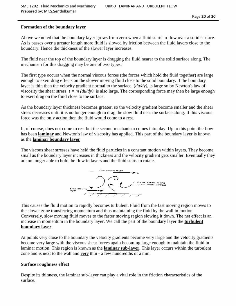
The viscous shear stresses have held the fluid particles in a constant motion within layers. They become

small as the boundary layer increases in thickness and the velocity gradient gets smaller. Eventually they

are no longer able to hold the flow in layers and the fluid starts to rotate.

This causes the fluid motion to rapidly becomes turbulent. Fluid from the fast moving region moves to

the slower zone transferring momentum and thus maintaining the fluid by the wall in motion.

Conversely, slow moving fluid moves to the faster moving region slowing it down. The net effect is an

increase in momentum in the boundary layer. We call the part of the boundary layer the turbulent

boundary layer.

At points very close to the boundary the velocity gradients become very large and the velocity gradients

become very large with the viscous shear forces again becoming large enough to maintain the fluid in

laminar motion. This region is known as the laminar sub-layer. This layer occurs within the turbulent

zone and is next to the wall and very thin - a few hundredths of a mm.

Surface roughness effect

Despite its thinness, the laminar sub-layer can play a vital role in the friction characteristics of the

surface.


Page 21 of 30

This is particularly relevant when defining pipe friction - as will be seen in more detail in the level 2

module. In turbulent flow if the height of the roughness of a pipe is greater than the thickness of the

laminar sub-layer then this increases the amount of turbulence and energy losses in the flow. If the

height of roughness is less than the thickness of the laminar sub-layer the pipe is said to be smooth and it

has little effect on the boundary layer.

In laminar flow the height of roughness has very little effect

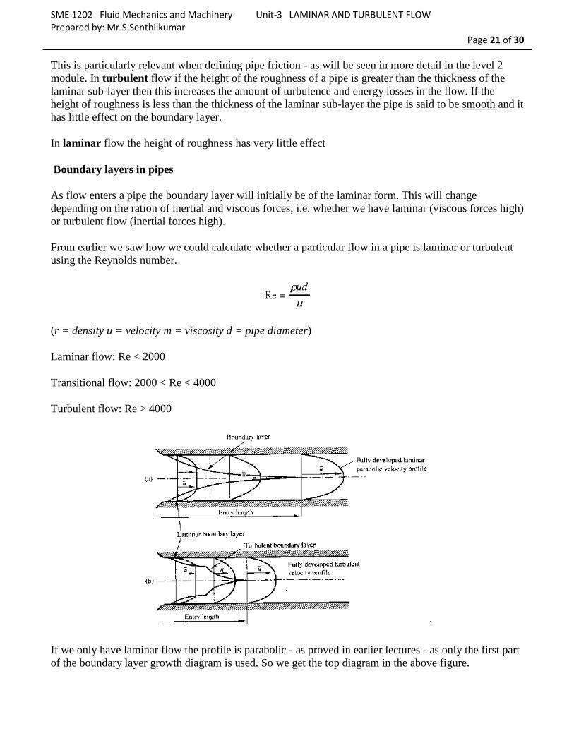
Boundary layers in pipes

As flow enters a pipe the boundary layer will initially be of the laminar form. This will change

depending on the ration of inertial and viscous forces; i.e. whether we have laminar (viscous forces high)

or turbulent flow (inertial forces high).

From earlier we saw how we could calculate whether a particular flow in a pipe is laminar or turbulent

using the Reynolds number.

(r = density u = velocity m = viscosity d = pipe diameter)

Laminar flow: Re < 2000

Transitional flow: 2000 < Re < 4000

Turbulent flow: Re > 4000

If we only have laminar flow the profile is parabolic - as proved in earlier lectures - as only the first part

of the boundary layer growth diagram is used. So we get the top diagram in the above figure.


Page 22 of 30

If turbulent (or transitional), both the laminar and the turbulent (transitional) zones of the boundary layer

growth diagram are used. The growth of the velocity profile is thus like the bottom diagram in the above

figure.

Once the boundary layer has reached the centre of the pipe the flow is said to be fully developed. (Note

that at this point the whole of the fluid is now affected by the boundary friction.)

The length of pipe before fully developed flow is achieved is different for the two types of flow. The

length is known as the entry length.

Laminar flow entry length 120 diameter

Turbulent flow entry length 60 diameter

Boundary layer separation Convergent flows: Negative pressure gradients

If flow over a boundary occurs when there is a pressure decrease in the direction of flow, the fluid will

accelerate and the boundary layer will become thinner.

This is the case for convergent flows.

The accelerating fluid maintains the fluid close to the wall in motion. Hence the flow remains stable and

turbulence reduces. Boundary layer separation does not occur.

Divergent flows: Positive pressure gradients

When the pressure increases in the direction of flow the situation is very different. Fluid outside the

boundary layer has enough momentum to overcome this pressure which is trying to push it backwards.

The fluid within the boundary layer has so little momentum that it will very quickly be brought to rest,

and possibly reversed in direction. If this reversal occurs it lifts the boundary layer away from the

surface as shown below.


Page 23 of 30

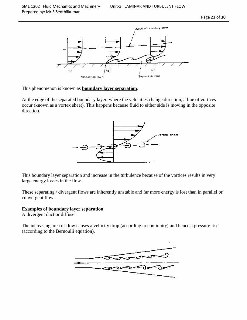
This phenomenon is known as boundary layer separation.

At the edge of the separated boundary layer, where the velocities change direction, a line of vortices

occur (known as a vortex sheet). This happens because fluid to either side is moving in the opposite

direction.

This boundary layer separation and increase in the turbulence because of the vortices results in very

large energy losses in the flow.

These separating / divergent flows are inherently unstable and far more energy is lost than in parallel or

convergent flow.

Examples of boundary layer separation A divergent duct or diffuser

The increasing area of flow causes a velocity drop (according to continuity) and hence a pressure rise

(according to the Bernoulli equation).


Page 24 of 30

Increasing the angle of the diffuser increases the probability of boundary layer separation. In a Venturi

meter it has been found that an angle of about 6 provides the optimum balance between length of meter

and danger of boundary layer separation which would cause unacceptable pressure energy losses.

Tee-Junctions

Assuming equal sized pipes, as fluid is removed, the velocities at 2 and 3 are smaller than at 1, the

entrance to the tee. Thus the pressure at 2 and 3 are higher than at 1. These two adverse pressure

gradients can cause the two separations shown in the diagram above.

Y-Junctions

Tee junctions are special cases of the Y-junction with similar separation zones occurring. See the

diagram below.

Downstream, away from the junction, the boundary layer reattaches and normal flow occurs i.e. the

effect of the boundary layer separation is only local. Nevertheless fluid downstream of the junction will

have lost energy.

Bends


Page 25 of 30

Two separation zones occur in bends as shown above. The pressure at b must be greater than at a as it

must provide the required radial acceleration for the fluid to get round the bend. There is thus an adverse

pressure gradient between a and b so separation may occur here.

Pressure at c is less than at the entrance to the bend but pressure at d has returned to near the entrance

value - again this adverse pressure gradient may cause boundary layer separation.

Flow past a cylinder

The pattern of flow around a cylinder varies with the velocity of flow. If flow is very slow with the

Reynolds number (r v diameter/m) less than 0.5, then there is no separation of the boundary layers as the

pressure difference around the cylinder is very small. The pattern is something like that in the figure

below.

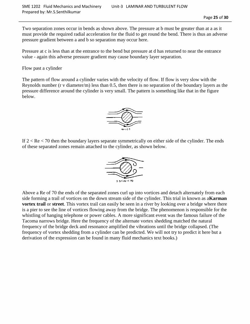
If 2 < Re < 70 then the boundary layers separate symmetrically on either side of the cylinder. The ends

of these separated zones remain attached to the cylinder, as shown below.

Above a Re of 70 the ends of the separated zones curl up into vortices and detach alternately from each

side forming a trail of vortices on the down stream side of the cylinder. This trial in known as aKarman

vortex trail or street. This vortex trail can easily be seen in a river by looking over a bridge where there

is a pier to see the line of vortices flowing away from the bridge. The phenomenon is responsible for the

whistling of hanging telephone or power cables. A more significant event was the famous failure of the

Tacoma narrows bridge. Here the frequency of the alternate vortex shedding matched the natural

frequency of the bridge deck and resonance amplified the vibrations until the bridge collapsed. (The

frequency of vortex shedding from a cylinder can be predicted. We will not try to predict it here but a

derivation of the expression can be found in many fluid mechanics text books.)


Page 26 of 30

Looking at the figure above, the formation of the separation occurs as the fluid accelerates from the

centre to get round the cylinder (it must accelerate as it has further to go than the surrounding fluid). It

reaches a maximum at Y, where it also has also dropped in pressure. The adverse pressure gradient

between here and the downstream side of the cylinder will cause the boundary layer separation if the

flow is fast enough, (Re > 2.)

Aerofoil

Normal flow over a aerofoil (a wing cross-section) is shown in the figure below with the boundary

layers greatly exaggerated.

The velocity increases as air it flows over the wing. The pressure distribution is similar to that shown

below so transverse lift force occurs.

If the angle of the wing becomes too great and boundary layer separation occurs on the top of the

aerofoil the pressure pattern will change dramatically. This phenomenon is known as stalling.


Page 27 of 30

When stalling occurs, all, or most, of the 'suction' pressure is lost, and the plane will suddenly drop from

the sky! The only solution to this is to put the plane into a dive to regain the boundary layer. A

transverse lift force is then exerted on the wing which gives the pilot some control and allows the plane

to be pulled out of the dive.

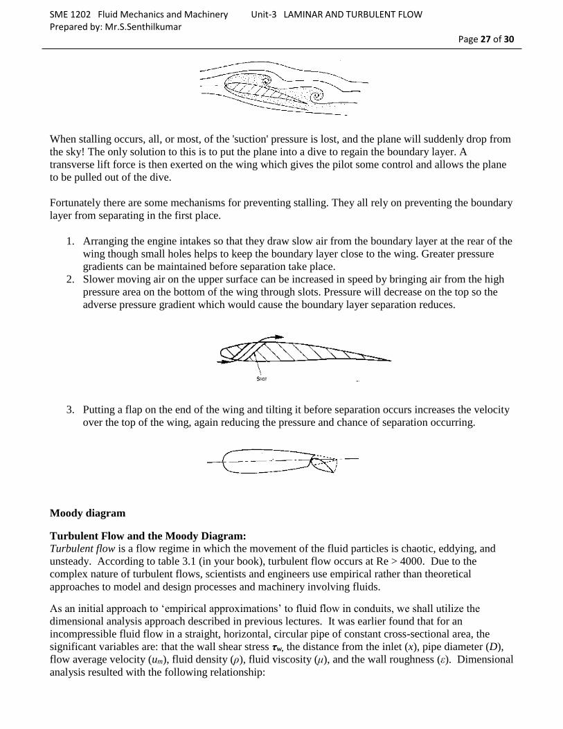
Fortunately there are some mechanisms for preventing stalling. They all rely on preventing the boundary

layer from separating in the first place.

1. Arranging the engine intakes so that they draw slow air from the boundary layer at the rear of the

wing though small holes helps to keep the boundary layer close to the wing. Greater pressure

gradients can be maintained before separation take place.

2. Slower moving air on the upper surface can be increased in speed by bringing air from the high

pressure area on the bottom of the wing through slots. Pressure will decrease on the top so the

adverse pressure gradient which would cause the boundary layer separation reduces.

3. Putting a flap on the end of the wing and tilting it before separation occurs increases the velocity

over the top of the wing, again reducing the pressure and chance of separation occurring.

Moody diagram

Turbulent Flow and the Moody Diagram: Turbulent flow is a flow regime in which the movement of the fluid particles is chaotic, eddying, and

unsteady. According to table 3.1 (in your book), turbulent flow occurs at Re > 4000. Due to the

complex nature of turbulent flows, scientists and engineers use empirical rather than theoretical

approaches to model and design processes and machinery involving fluids.

As an initial approach to ‘empirical approximations’ to fluid flow in conduits, we shall utilize the

dimensional analysis approach described in previous lectures. It was earlier found that for an

incompressible fluid flow in a straight, horizontal, circular pipe of constant cross-sectional area, the

significant variables are: that the wall shear stress τw, the distance from the inlet (x), pipe diameter (D),

flow average velocity (um), fluid density (ρ), fluid viscosity (μ), and the wall roughness (ε). Dimensional

analysis resulted with the following relationship:


Page 28 of 30

The function , which varies with the relative roughness and Reynolds number is designated f, the

friction factor.

Expressing the above relationship in terms of f, we have:

Other versions in more common use are the Fanning friction factor:

Piping and Pumping Problems Upward flow in an inclined pipe is depicted in Fig. 3.9 (below). A steady-state momentum balance in

the direction of flow on the fluid in the pipe gives:

Rearranging the substituting for wall shear stress in terms of the friction factor (f) gives:

An alternative and somewhat more generally useful form of the above equation is obtained by

investigating the frictional dissipation per unit mass. Rearrangement of the preceding equation yields:

But the overall (incompressible) energy balance for fluid flow in a pipe is:


Page 29 of 30

Realizing that the change in kinetic energy is zero (constant cross section) and there is no work

involved, then by comparing the preceding two equations, we obtain:

A result that is valid for LAMINAR or TURBULENT flow.

For the special case of LAMINAR flow, from the analysis obtained earlier (Hagen-Poiseuille equation),

we know that:

Since , the friction factor for laminar flow is therefore:

Experimentally, the friction factor depends on the Re and (if turbulent) on the pipe relative roughness.

The relationship between the friction factor, Re, and relative roughness is schematically presented in

Figure. This diagram is generally referred to as the Moody Diagram.

Example


Page 30 of 30

Water (T= 20 oC) flows at a rate of 0.05 m3/s in a 20 cm asphalted cast-iron pipe. What is the

head loss (frictional losses) per kilometer of pipe?

Solution

1. Calculate the average flow velocity using the continuity equation 2. Calculate the Reynolds number (to determine wither the flow is laminar or turbulent) 3. Calculate the relative roughness

4. Look up the f (friction factor) using the Moody Diagram

Average velocity:

Reynolds number:

Friction factor (f):

Pipe material equivalent roughness (asphalted cast-iron pie) = 0.12 mm

Relative roughness =

fF from diagram ~ 0.00475

Frictional loss:

Documents

UNIT 3 LAMINAR AND TURBULENT FLOW Orifice · 2016-09-12 · Mathematically coefficient of contraction, The value of Coefficient of contraction varies slightly with the available head