Embed Size (px)
Citation preview
91
Spreadsheet UNIT 3 SPREADSHEET
Structure Page No.
3.0 Introduction 92
3.1 Objectives 93
3.3 What is a Spreadsheet ? 93
3.3 Excel Basics 93
3.3.1 Starting Excel 94
3.3.2 Commands and Resources in Excel Window 95
3.3.3 Setting Up in Your Excel Environment 97
3.3.4 Creating a New Workbook 100
3.3.5 Opening an Existing Workbook 101
3.3.6 Saving a Existing Document 101
3.3.7 Working with Multiple Workbooks 102
3.3.8 Closing a Workbook 102
3.3.9 Closing Microsoft Excel 102
3.4 Entering, Editing and Formatting Data 102
3.4.1 Moving around the Worksheet 103
3.4.2 Selecting Cells, Rows or Columns 104
3.4.2.1 Selecting Cells 104
3.4.3 Entering Data 105
3.4.4 Deleting Data 105
3.4.5 Editing Data 105
3.4.6 Working with Cells, Rows and Columns 106
3.4.7 Data and Formatting 110
3.5 Formulas and Functions 115
3.5.1 Formulas 116
3.5.1.1 Create a Simple Formulas 116
3.5.1.2 Create a Simple Formulas using Point and Click Method 116
3.5.2 Using Cell References 117
3.5.3 Linking Worksheets 117
3.5.4 Functions 118
3.5.4.1 Function Library 118
3.5.4.2 Insert a Function 118
3.6 Working with Worksheets 116
3.6.1 Name a Worksheet 119
3.6.2 Insert a New Worksheet 120
3.6.3 Delete a Worksheet 120
92
Lab Course
3.6.4 Grouping Worksheets 120
3.6.5 Ungrouping Worksheets 121
3.6.6 Reposition Worksheets in a Workbook 121
3.6.7 Hide Worksheets 121
3.6.8 Formatting and Printing the Workbook 122
3.7 Working with Tables and Charts 124
3.7.1 Tables 124
3.7.1.1 Create Table 125
3.7.1.2 Sort Data 126
3.7.1.3 Filter Data 126
3.7.2 Charts 127
3.7.2.1 Add Data 128
3.7.2.2 Create Chart 128
3.7.2.3 Apply Layout 128
3.7.2.4 Add Labels 129
3.7.2.5 Switch Data 129
3.7.2.6 Change Chart Type, Chart Style or Data Range 129
3.7.2.7 Move the Chart to a Different Worksheet 129
3.8 Other Useful Excel Features 129
3.8.1 Conditional Formating 129
3.8.2 Freeze Rows and Columns 130
3.8.3 Find and Replace 130
3.8.4 Add Comments 131
3.8.5 Protect Worksheet 131
3.8.6 Convert Text to Columns 130
3.9 Summary 133
3.10 Lab Exercise 133
3.11 Further Readings 137
3.0 INTRODUCTION
Every business has numerical tasks to be performed, be it related to accounts,
taxes, sales or budgeting. Businesses also need graphs and charts for analysis and
projections. At homes, we track our own budgets and investments. Mathematics
and Engineering students deal with big numbers, formulas and calculations.
Almost all of us deal with tables, data and calculations in some or the other form.
There are many software packages available to assists us in all these number
based functions. Electronic spreadsheet is most common of them.
In this unit, we will study how we can use electronic spreadsheet to store,
maintain, manage, manipulate and organize our data for budgeting, analysis and
93
Spreadsheet planning purposes or how we can use to it track students performance, weather
data or inventory and maintain friends list, customer list, etc.
3.1 OBJECTIVES
After going through this unit, you will be able to ;
learn what a Spreadsheet is and how to use it;
create, edit, save, preview and print Workbooks;
format worksheets with different settings such as margins, headers or footers;
store, search, retrieve, sort and filter tabular data;
manage and Manipulate data using functions and formulas; and
create graphical charts and perform analysis functions.
3.3 WHAT IS A SPREADSHEET ?
Spreadsheet is basically a grid consisting of horizontal rows and vertical columns.
This format has traditionally been used in accounting to present book-keeping
ledgers.
Electronic spreadsheet is a computer application that simulates the paper
worksheet to organize data into rows and columns and stores various types of
data.
Each intersection of rows and columns is called a cell where the data is stored to
be used in calculations within the spreadsheet. Electronic spreadsheets have lot of
in built features and tools such as functions, formulas, charts, and data analysis
tools that make it easier to work with large amount of data. It provides ability to
perform mathematical calculations quickly and has flexibility to perform quick
recalculation in case of any data change.
Electronic spreadsheets can be used in any area or field that works with numbers
and are commonly found in the accounting, budgeting, sales forecasting, financial
analysis and scientific fields. It can be used to create and maintain a list, store
database records, create charts or graphs, compare numerical or financial data.
There are quite a few electronic spreadsheet programs available like Excel,
OpenOffice Calc or Google spreadsheets. We will consider MS Excel 3007 for
our study. It comes bundled in MS Office which is an office automation tool.
3.3 EXCEL BASICS
In this section, we will cover how to start Excel, open, save and close a workbook
and what different parts of Excel Window stand for.
94
Lab Course
3.3.1 Starting Excel
You can start MS Excel by either of the following two ways:
Click on Start All ProgramMicrosoft Office Microsoft Office Excel
3007.
Double click on the MS Excel icon on the desktop (if you have one).
When Excel opens, a new document (called Workbook in Excel) with default
name as Book1 is opened. For each additional workbook you open, the number
increases by one. Please note that you can open more than one workbook at a
time. By default each workbook contains three worksheets. You may increase or
decrease the number of worksheets in a workbook. How we do it, we will learn
later in this unit.
You may also start Excel by clicking on a workbook saved on your hard drive.
Excel will open automatically and the workbook will be displayed in the Excel
window.
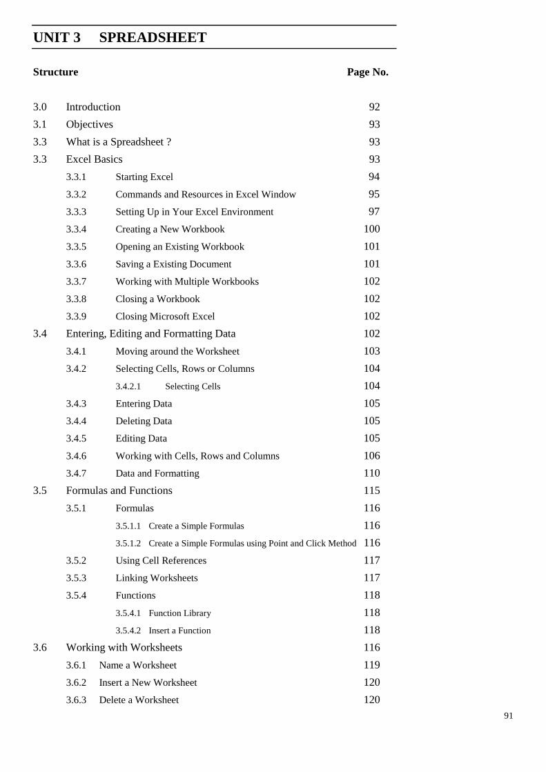
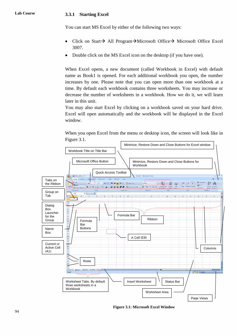
When you open Excel from the menu or desktop icon, the screen will look like in
Figure 3.1.
Figure 3.1: Microsoft Excel Window
Quick Access Toolbar
Microsoft Office Button
Workbook Title on Title Bar
Minimize, Restore Down and Close Buttons for Excel window
Status Bar
Ribbon
Tabs on the Ribbon
Help Button
Group on Tab
Formula Bar
Dialog Box Launcher for the Group
Vertical Scroll Bar
Minimize, Restore Down and Close Buttons for Workbook
A Cell (E8)
Rows
Columns
Insert Worksheet Worksheet Tabs. By default three worksheets in a Workbook
Expand Formula Bar
Current or Active Cell (A1)
Name Box
Zoom Tool
Page Views
Worksheet Area
Formula Bar Buttons
95
Spreadsheet 3.3.2 Commands and Resources in Excel Window
Let us familiarize ourselves with the key commands and resources in Excel
Window:
The Microsoft Office Button
It is the button in the upper-left corner of the Excel Window. When you click on
the button, it displays a menu that can be used to create a new workbook, open an
existing workbook, save a workbook, print and perform many other tasks.
The Quick Access Toolbar
It is present next to the Microsoft Office Button on the top. It provides you access
to the commands you frequently use. By default Following appear on the Quick
Access Toolbar:
Save: To save your file (you may also press keyboard button ( Ctrl+S).
Undo: To rollback the action that you last took (Ctrl+Z).
Redo: To reapply the action you rolled back or to repeat an action (Ctrl+Y).
The Title Bar
It is next to the Quick Access toolbar at the top. It displays the title of the
workbook on which you are currently working. By default, the first new
workbook is named as Book1. For each additional workbook you open, the
number increases by one. You may save the workbooks by any legal filename you
want.
The Ribbon
The Ribbon is the panel at the top portion of the document, right below the Title
Bar. To begin with it has following seven tabs:
Home: It has basic commands for creating, formatting and editing the
spreadsheets. It has controls for working with the clipboard, fonts, alignment,
number, styles, cells and editing.
Insert: It has commands for inserting tables, pictures, shapes, other
illustrations, links, charts, header, footer, etc.
Page Layout: The commands here help to set the layout of the spreadsheet,
apply a theme to set the overall look, set the margins, orientation, size,
backgrounds, etc.
96
Lab Course
Formulas: It has commands that help you use different formulas and
functions.
Data: Has commands to import, query, view data from external sources, sort,
filter or manage data.
Review: Has commands to add comments, protect sheet, protect workbook,
share workbook, etc.
View: Helps to change the display of the worksheet area.
Besides these basic tabs, additional tabs appear from time to time, depending on
the context we are working in. These tabs are called contextual tabs. For example,
if you select a chart, a Chart Tools contextual tab appears that has commands to
help you design and format the chart. These contextual tabs appear in a different
colour to make them easy to spot.
The commands on each tab are organized into groups. Hence, a group is a
collection of logically related command buttons that you can use to manage a
Worksheet. Commonly used features are displayed on the Ribbon and additional
options can be accessed through the dialog box launcher at the bottom-right
corner of each group.
The Formula Bar
The formula bar is divided into three sections:
Name Box: Located on the left most side of the formula bar, it displays the
address of the current cell
Formula Bar Buttons: Middle section of the formula bar with indented circle on
the left (to increase or decrease the size of the name box) and function wizard
(labeled fx) on the right. When you start entering data in the cell, Cancel ( ) and
Enter ( ) buttons also appear.
Cell Contents: Right side of the formula bar displays the cell entries.
The Worksheet Area
The worksheet area displays all the cells. It is in the cells that you enter, format or
edit your data.
The Status Bar
The Status bar appears at the very bottom of the Excel window and provides such
information as the sum, average, minimum, and maximum value of selected
numbers. You can change what displays on the Status bar by right-clicking on the
97
Spreadsheet Status bar and selecting the options you want from the Customize Status Bar
menu. You click a menu item to select it. You click it again to deselect it. A check
mark next to an item means the item is selected.
3.3.3 Setting up Your Excel Environment
Before you begin working on your spreadsheet, you may want to set up your
Excel environment and become familiar with a few key tasks such as how to
maximize and minimize the Ribbon, configure the Quick Access toolbar, display/
hide the formula bar, change page views etc.
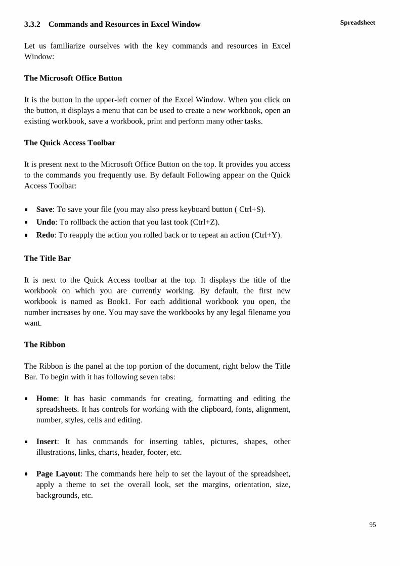
Minimize and Maximize the Ribbon
Right click anywhere in the main menu
Select Minimize the Ribbon in the menu that appears. This will toggle the
Ribbon on and off.
Figure 3.2 : Minimize the Ribbon
The check mark beside ‘Minimize the Ribbon’ option indicates the feature is
active. You may choose to use this option, if you prefer not to use the Ribbon, but
use different menus and keyboard shortcuts.
This menu also has option to Show Quick Access Toolbar Below the Ribbon,
instead of at the top. You can also Customize Quick Access Toolbar using the
option available in this menu. Choosing this option displays the window as shown
in figure 3.
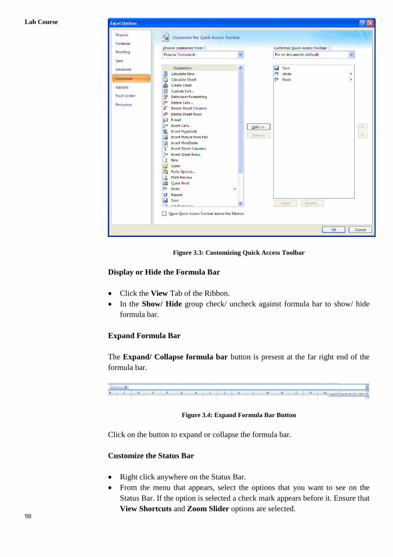
Add Commands to Quick Access Toolbar
Click the arrow (customize quick access toolbar) to the right of the Quick
Access toolbar.
Select the command you wish to add from the drop down menu. The
command will appear in the Quick Access Toolbar
You can also select More commands… from the menu to open the screen as
shown in Figure 3.3. Here you can one by one add commands to the toolbar or
remove commands from the toolbar to make specific features easily accessible.
98
Lab Course
Figure 3.3: Customizing Quick Access Toolbar
Display or Hide the Formula Bar
Click the View Tab of the Ribbon.
In the Show/ Hide group check/ uncheck against formula bar to show/ hide
formula bar.
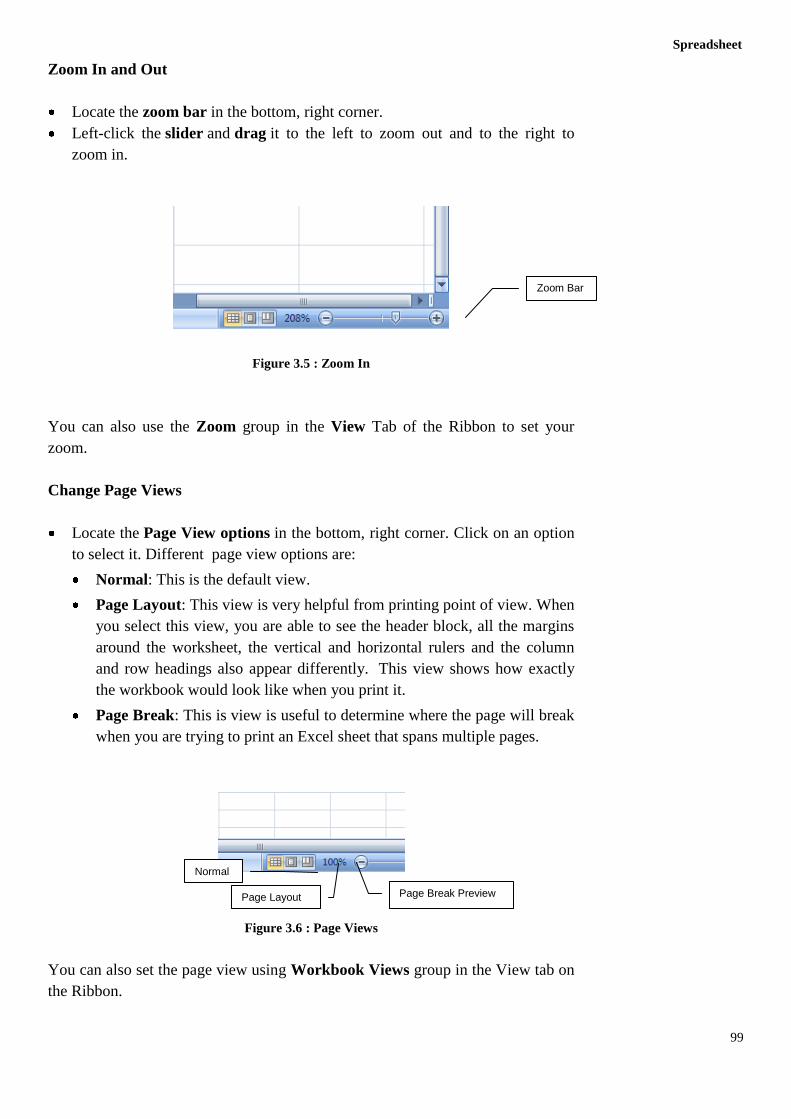
Expand Formula Bar
The Expand/ Collapse formula bar button is present at the far right end of the
formula bar.
Figure 3.4: Expand Formula Bar Button
Click on the button to expand or collapse the formula bar.
Customize the Status Bar
Right click anywhere on the Status Bar.
From the menu that appears, select the options that you want to see on the
Status Bar. If the option is selected a check mark appears before it. Ensure that
View Shortcuts and Zoom Slider options are selected.
99
Spreadsheet
Zoom In and Out
Locate the zoom bar in the bottom, right corner.
Left-click the slider and drag it to the left to zoom out and to the right to
zoom in.
Figure 3.5 : Zoom In
You can also use the Zoom group in the View Tab of the Ribbon to set your
zoom.
Change Page Views
Locate the Page View options in the bottom, right corner. Click on an option
to select it. Different page view options are:
Normal: This is the default view.
Page Layout: This view is very helpful from printing point of view. When
you select this view, you are able to see the header block, all the margins
around the worksheet, the vertical and horizontal rulers and the column
and row headings also appear differently. This view shows how exactly
the workbook would look like when you print it.
Page Break: This is view is useful to determine where the page will break
when you are trying to print an Excel sheet that spans multiple pages.
Figure 3.6 : Page Views
You can also set the page view using Workbook Views group in the View tab on
the Ribbon.
Zoom Bar
Normal
Page Layout Page Break Preview
100
Lab Course
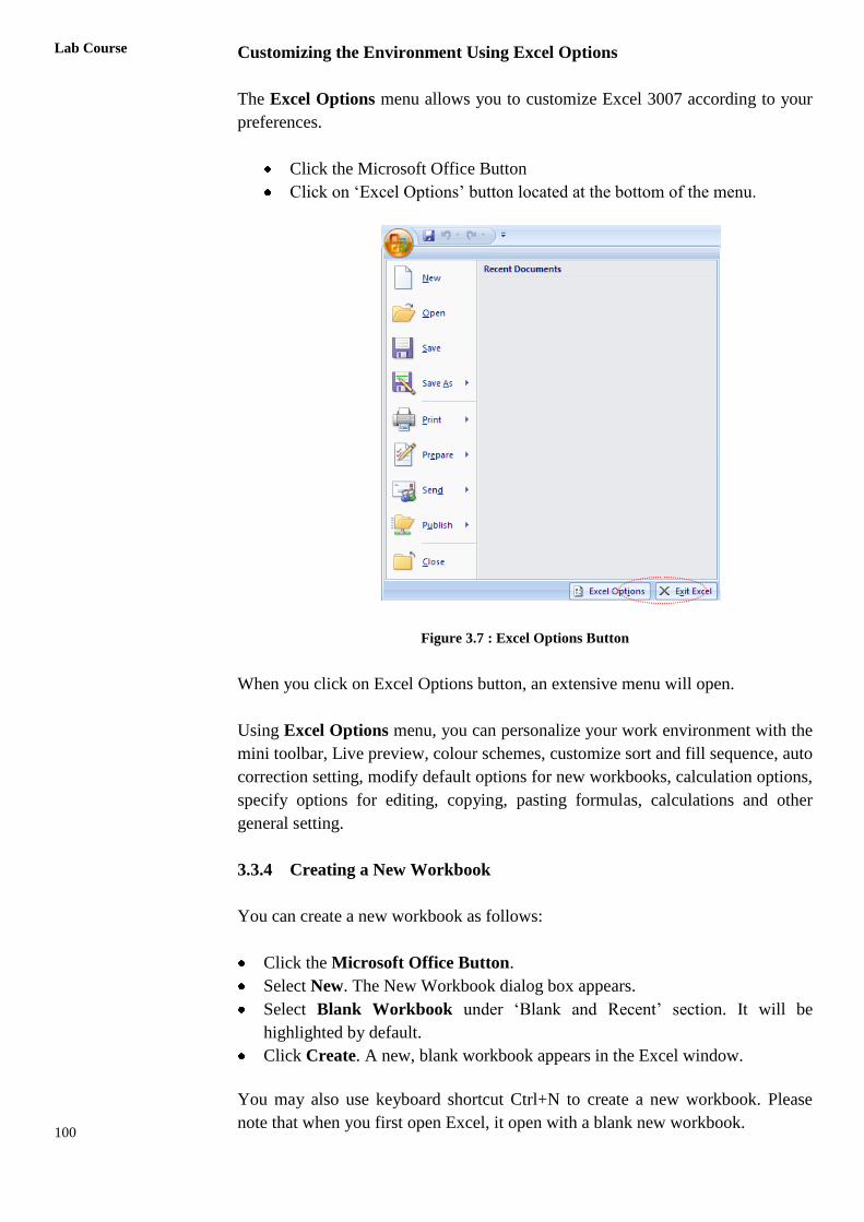
Customizing the Environment Using Excel Options
The Excel Options menu allows you to customize Excel 3007 according to your
preferences.
Click the Microsoft Office Button
Click on ‘Excel Options’ button located at the bottom of the menu.
Figure 3.7 : Excel Options Button
When you click on Excel Options button, an extensive menu will open.
Using Excel Options menu, you can personalize your work environment with the
mini toolbar, Live preview, colour schemes, customize sort and fill sequence, auto
correction setting, modify default options for new workbooks, calculation options,
specify options for editing, copying, pasting formulas, calculations and other
general setting.
3.3.4 Creating a New Workbook
You can create a new workbook as follows:
Click the Microsoft Office Button.
Select New. The New Workbook dialog box appears.
Select Blank Workbook under ‘Blank and Recent’ section. It will be
highlighted by default.
Click Create. A new, blank workbook appears in the Excel window.
You may also use keyboard shortcut Ctrl+N to create a new workbook. Please
note that when you first open Excel, it open with a blank new workbook.

101
Spreadsheet If you want to create a new document from a template, explore the templates and
choose one that fits your needs, instead of choosing new blank workbook.
3.3.5 Opening an Existing Workbook
You can open an existing document in one of the following ways:
Click the Microsoft Office Button.
Select Open. Select the required workbook in the dialog box.
OR
Use keyboard shortcut Ctrl+O to select and open an existing document.
OR
If you have recently used workbook then
Click the Microsoft Office Button.
Choose from the Recent Documents section.
OR
Go to Windows Explorer. Find your document.
Right mouse click on the document and select Open.
3.3.6 Saving a Existing Document
Click the Microsoft Office Button.
Select Save from the menu.
OR
Use keyboard shortcut Ctrl+S
OR
Use Save on the Quick Access Toolbar
On using any of these options, the workbook is saved in its current location with
the same file name. If you are saving the workbook for the first time, then Save
As dialog box appears which accepts the workbook name and location where it is
to be saved.
Using Save As Option
You may use Save As option as below:
Click the Microsoft Office Button.
Select Save As from the menu. The Save As dialog box appears.
Select the location where you wish to save the workbook.
Enter the name for the workbook.
Click the Save button
The Save As option can be used to:
102
Lab Course
Create a backup copy of the workbook by saving it at another location or by
different name.
Save the workbook in a format that is fully compatible with Excel97-3003
Save the workbook as macro-enabled or binary workbook.
3.3.7 Working with Multiple Workbooks
Multiple workbooks can be opened simultaneously if there is such a need. To see
the list of open workbooks:
Click on View tab of the Ribbon
Click on Switch Windows in the Window group. A drop down list of all open
workbooks is displayed.
The current workbook has a checkmark besides its name. You may select any
workbook from the list to make it current.
3.3.8 Closing a Workbook
To close a workbook:
Click the Microsoft Office Button.
Select Close from the menu.
The current workbook closes. The next document in the list becomes current. If
there is no other open document, then only Excel window is there.
3.3.9 Closing Microsoft Excel
Click the Microsoft Office Button. A menu appears.
Click Close. Excel closes.
3.4 ENTERING, EDITING AND FORMATTING DATA
Excel treats different types of data differently. You enter all kinds of data in a cell
in the worksheet. An Excel workbook can hold any number of worksheets and
each worksheet is made up of more than seventeen billion cells. Each cell can
hold any of the following three types of data:
A numeric value : It can be numbers (example 300.40), dates (example
4-Feb-2011) or times (example 3:35 am). There are many different format
options available in Excel for the display of numerical values.
Text : Text in Excel can be used as labels for values, headings for columns or
worksheet or for any kind of instructions. Text that begins with a number is
still considered as text.

103
Spreadsheet A Formula : Formulas can be entered in a cell where eventually the result of
the formula is displayed. We will study more about formulas later in this unit.
A worksheet can also hold charts, diagrams, pictures and other objects. These
objects aren’t contained in cells. Rather, they reside on the worksheet’s draw
layer, which is an invisible layer on top of each worksheet.
In order to enter or edit data in a cell, that cell must be current. Excel indicates
that a cell is current in following ways:
A dark black border (called the cell cursor) appears around the cell.
The cell address appears in the Name box of the formula bar. A cell address
is combination of Column Letter(s) and Row number that intersect at that cell
position. For example, if the cell address is A3, it means it is at the
intersection of column A and row 3.
The cell column heading (letters) and row heading (number) is shaded for that
particular cell.
3.4.1 Moving around the Worksheet
Excel has many ways to move the cell cursor around the worksheet to the cell
where you want to enter new data or edit existing data:
Click the desired cell, provided the cell is displayed within the visible section
of the worksheet area.
In case, cell is not visible, then you may use horizontal or vertical scroll bars
to move to that part of the worksheet that contains the desired cell.
Press F5 to open the Go To dialog box. Type the cell address in the reference
and press Enter or click OK. The cell cursor moves to the desired address.
Press CTRL+G. This again opens Go To dialog box.
Click in the Name box of formula bar and enter the address of the desired cell.
Preas Enter. Cursor moves to the specified cell.
You can also use the arrow and tab keys as specified below to move the cell
cursor to the desired cell:
104
Lab Course
To Move Keys to Press
One cell on right Tab or right arrow key
One cell on left Shift+Tab or left arrow key
One cell up Up arrow key
One cell down Down arrow key
To cell A1 Ctrl+Home
To last cell with any data (last column and last
row)
Ctrl+End
Up or Down one screen PgUp or PgDn
First cell of the current row Home
3.4.2 Selecting Cells, Rows or Columns
If you wish to perform a function on a group of cells, you must first select those
cells by highlighting them.
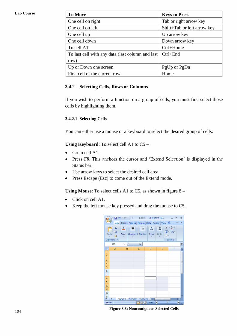
3.4.2.1 Selecting Cells
You can either use a mouse or a keyboard to select the desired group of cells:
Using Keyboard: To select cell A1 to C5 –
Go to cell A1.
Press F8. This anchors the cursor and ‘Extend Selection’ is displayed in the
Status bar.
Use arrow keys to select the desired cell area.
Press Escape (Esc) to come out of the Extend mode.
Using Mouse: To select cells A1 to C5, as shown in figure 8 –
Click on cell A1.
Keep the left mouse key pressed and drag the mouse to C5.
Figure 3.8: Noncontiguous Selected Cells
105
Spreadsheet You can also select noncontiguous area of the worksheet using mouse. Press Ctrl
key along with the left mouse key while dragging to select the cells.
To select a particular row or a column, just click on that particular row or column
heading. For example, if you want to select row number 3, then just click on
number 3 in the row heading and the entire row will be highlighted. When you
take the cursor over the row heading, then it changes to a right arrow. Similarly,
when you take the cursor over the column heading, then it changed to a down
arrow.
3.4.3 Entering Data
There are different ways to enter data in Excel: in an active cell or in the formula
bar.
To enter data in an active cell:
Click in the cell where you want the data.
Begin typing. Note that the text appears in formula bar also.
To enter data into the formula bar:
Click the cell where you would like the data
Place the cursor in the Formula Bar
Type in the data in the formula bar
Please note that you can use Alt+Enter to go to next line within a cell.
Alt+Enter in a cell works similar to Enter key in a word document.
3.4.4 Deleting Data
Select the cell(s).
Press the Delete key to delete the entire contents of a cell(s).
OR
Double click in a cell. The insertion point appears in the cell.
Press Backspace to delete one character at a time. Press Enter to confirm
changes.
You can also make changes to and delete text from the formula bar. Just select the
cell and place your insertion point in the formula bar and use backspace or select
the whole text and use delete.
3.4.5 Editing Data
To change entire contents of a cell:
106
Lab Course
Select the cell and start typing the new data.
Press Enter to confirm the change.
To modify a part of the cell,
Select the cell and switch to edit mode. You can switch to edit mode by
following ways:
Press F3 once you have selected the cell. The Status changes to ‘Edit’
from ‘Ready’ in the status bar.
OR
Double click in the cell to switch to edit mode.
Once you have made your changes, press Enter to confirm changes or press Esc to
cancel changes.
You can also make changes in the Formula bar. Select cell. Click in the formula
bar. Make the required changes. Press Enter to confirm or press Esc to cancel
changes.
3.4.6 Working with Cells, Rows and Columns
Copy/ Cut and Paste
If you need to duplicate data in some cell(s), you can use copy & paste option. In
case you need to move the data from one cell to another, then you use cut & paste
option.
To copy data:
Select the cell(s) that you wish to copy. This is the source location.
On the Clipboard group of the Home tab, click Copy OR use Ctrl+C OR
select Copy option from menu that appears when you right mouse click on the
selected cell(s). The border of the selected cell(s) will change appearance and
the data from the selected cell(s) is copied onto the clipboard.
To cut data:
Select the cell(s) that you wish to cut. This is the source location.
On the Clipboard group of the Home tab, click Cut OR use Ctrl+X OR select
Cut option from menu that appears when you right mouse click on the
selected cell(s). The border of the selected cell(s) will change appearance and
the data from the selected cell(s) is copied onto the clipboard.
To paste data:
Once you have copied or cut data from the source location, you paste it to the
destination location.
107
Spreadsheet Select the cell(s) where you would like to paste the data. This is the
destination location.
On the Clipboard group of the Home tab, click Paste OR use Ctrl+V OR use
right mouse click menu option. The source information will now appear in
the new destination cells.
If you use cut, then the information at the source location is removed
automatically after the paste operation has been performed. If you use copy, then
you have same information at both source and destination locations. Also, in case
of copy, the copied information remains selected with changed border (even after
the paste operation), until you perform next action or press Esc or double click the
selection to deselect it.
Drag and Drop
Drag and drop works similar to cut and paste that you move information from one
cell(s) to another. To drag and drop data from one point to another:
Select the cell(s) that you wish to move.
Position your mouse pointer near one of the outside edges of the selected
cells. The mouse pointer should change from a white, block cross to a black,
thin cross with 4 arrows.
Click and hold the mouse button and drag the cells to the new location. As
you drag the selected cells, the outline of the cells will change.
Release the mouse button and the information appears in the new location.
Please note that for drag and drop to work, it should be enabled in Excel Options.
Undo and Redo
Undo and Redo buttons are present in the Quick Access Toolbar. You can also
use keyboard shortcuts Ctrl+Z and Ctrl+Y for undo and redo respectively.
The undo command allows you to correct your mistakes in the worksheet. The
redo button becomes active when you use undo. It lets you undo what you have
undone. If you want to undo last action, then click on the Undo button. You can
also click the arrow key next to the Undo button to open a list of previous actions.
You can choose from the list to undo multiple actions at the same time. Please
note that once you have saved the file and made a change to the worksheet, then
you cannot undo any action performed before the save.
Insert Cell
You can insert a cell either above a cell or to the left of a cell. Keeping this in
mind,
Select the appropriate cell.
108
Lab Course
Click arrow on Insert command from Cells group in the Home tab. If you
click on the Insert button, a cell is inserted above the selected cell. But, if you
click the arrow then a menu opens.
Choose Insert Cells option. Insert dialog box opens.
Choose the appropriate option.
OR
Select the appropriate cell.
Right mouse click on the cell. A menu opens.
Select Insert… option from the menu. Insert dialog box opens.
Choose the appropriate option.
Insert Row or Column
You can insert a row above a particular row or a column to the left of a particular
column. While keeping this in mind,
Select a cell in the appropriate row/ column.
Either use right mouse click OR Insert command in Cells group of the Home
tab on the Ribbon (as done to insert a cell above).
In the Insert dialog box choose the appropriate option for row/ column.
OR
Press right mouse button on the row number (above which you want to insert
a row) in row heading on left of the worksheet OR press right mouse button
on the column letter in column heading (left of which you want to insert the
column) at the top of the worksheet. A menu opens.
Choose insert option from the menu. A row is added above the selected row
OR a column is added to the left of the selected column.
Delete Cell, Row or Column
To delete cells, rows, and columns:
Place the cursor in the cell, row, or column that you want to delete
Click the Delete button on the Cells group of the Home tab
Click the appropriate choice: Cell, Row, or Column
OR
Use right mouse click on the cell, row number in row heading or column
letter(s) in column heading.
Choose Delete option from the menu.
Modify Column Width
There are various ways that you can use to modify column width:
Position the cursor over the column line (line that divides the two columns) in
the column heading. A horizontal double arrow will appear.
109
Spreadsheet Click the mouse and drag the cursor to the right to increase the column width
or to the left to decrease the column width.
Release the mouse button.
OR
Click the column heading of a column you wish to modify. The entire column
will be highlighted.
Click the Format command in the Cells group on the Home tab. A menu will
appear.
Select Column Width to enter a specific column measurement
OR
select AutoFit Column Width to automatically adjust the column so all the
text will fit.
OR
Right mouse click the column heading. A menu will appear.
Select Column Width… from the menu.
Enter the specific column measurement.
Modify Row Height
There are multiple ways that you can use to modify row height:
Position the cursor over the row line (line that divides the two rows) in the
row heading for the row you want to modify. A vertical double arrow will
appear.
Click the mouse and drag the cursor upward to decrease the row height
or downward to increase the row height.
Release the mouse button.
OR
Click the row heading of a row you wish to modify. The entire row will
be highlighted.
Click the Format command in the Cells group on the Home tab. A menu will
appear.
Select Row Height to enter a specific row measurement OR select AutoFit
Row Height to automatically adjust the column so all the text will fit.
OR
Right mouse click the row heading. A menu will appear.
Select Row Height… from the menu.
Enter the specific row measurement.
Hide or Unhide Rows or Columns
To hide or unhide rows or columns:
110
Lab Course
Select the row or column you wish to hide or unhide.
Click the Format button on the Cells group of the Home tab. A menu
appears.
Under Visibility heading, click on Hide & Unhide option.
Choose the appropriate option from sub menu that appears: Hide Rows or
Hide Columns or Unhide Rows or Unhide Columns as per the requirements.
3.4.7 Data and Formatting
Auto Fill
Auto Fill feature fills cell data or series of data in a worksheet into a selected
range of cells. If you want the same data copied into the other cells, you only need
to enter data in one cell. If you want to have a series of data (for example, serial
number) fill in the first two cells in the series and then use the auto fill feature. To
use the Auto Fill feature:
Enter the required data in the cell. For example, if you wish to enter 1 in all
cells from A1 to A10, then just type 1 in cell A1. Similarly, if you wish to
enter numbers 1 to 10 in cells A1 to A10 then enter 1 in A1 and 3 in A3.
Now select the cell(s) with value(s) (just A1 OR both A1 and A3 depending
on the case)
Bring your cursor at the bottom right corner of the selection so that it changes
from large white cross to a small, thin, black cross. Now the cursor is
positioned over the fill handle.
Click your mouse at the fill handle and drag it till all the cells you want to fill
are selected (till A10 in our example).
Release the mouse button and all the selected cells are automatically filled.
You can use the fill handle to fill cells horizontally or vertically.
Aligning Values
In Excel, the data in a cell can be aligned both horizontally and vertically. The
default horizontal alignment is left for the text data and right for the numerical
data. Vertically, both text and numerical data are bottom aligned. You can change
the default alignments as per your requirement:
The steps to change alignment are:
Select the cell(s) for which alignment needs to be changed.
Choose horizontal/ vertical alignment command from the Alignment group in
the Home tab.
111
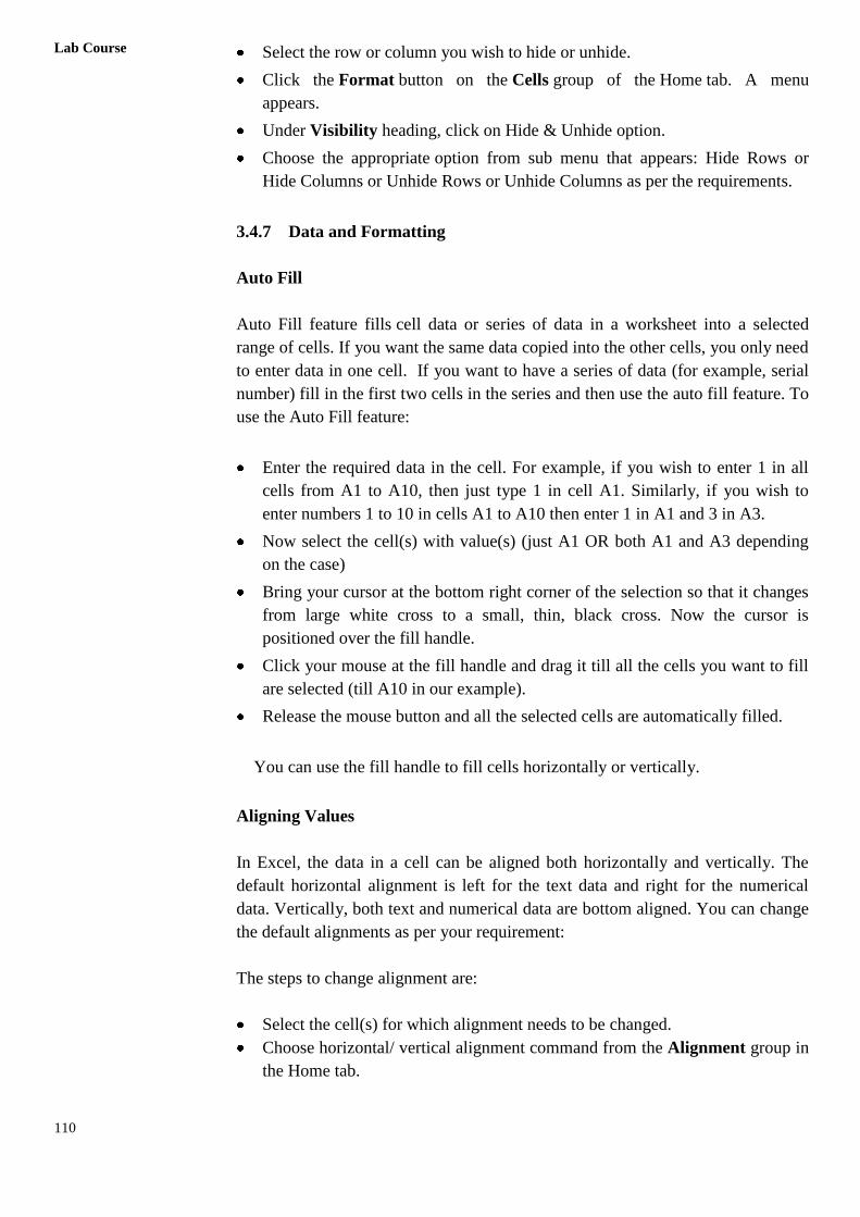
Spreadsheet In the Figure 3.9, you can see the how the data can be positioned in a cell by
choosing the appropriate combination of horizontal and vertical alignment values.
Figure 3.9: Horizontal and Vertical Alignments
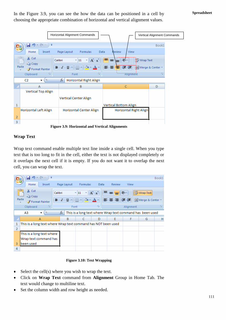
Wrap Text
Wrap text command enable multiple text line inside a single cell. When you type
text that is too long to fit in the cell, either the text is not displayed completely or
it overlaps the next cell if it is empty. If you do not want it to overlap the next
cell, you can wrap the text.
Figure 3.10: Text Wrapping
Select the cell(s) where you wish to wrap the text.
Click on Wrap Text command from Alignment Group in Home Tab. The
text would change to multiline text.
Set the column width and row height as needed.
Vertical Alignment Commands Horizontal Alignment Commands
112
Lab Course
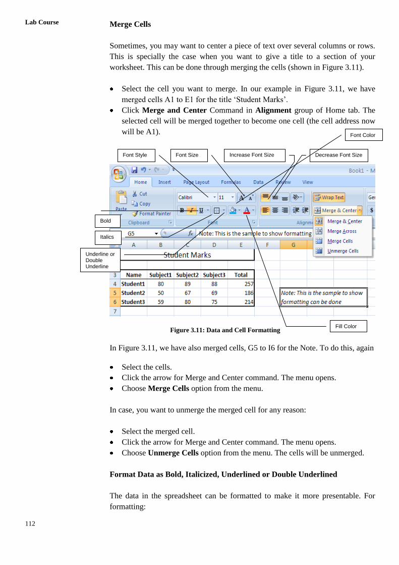
Merge Cells
Sometimes, you may want to center a piece of text over several columns or rows.
This is specially the case when you want to give a title to a section of your
worksheet. This can be done through merging the cells (shown in Figure 3.11).
Select the cell you want to merge. In our example in Figure 3.11, we have
merged cells A1 to E1 for the title ‘Student Marks’.
Click Merge and Center Command in Alignment group of Home tab. The
selected cell will be merged together to become one cell (the cell address now
will be A1).
Figure 3.11: Data and Cell Formatting
In Figure 3.11, we have also merged cells, G5 to I6 for the Note. To do this, again
Select the cells.
Click the arrow for Merge and Center command. The menu opens.
Choose Merge Cells option from the menu.
In case, you want to unmerge the merged cell for any reason:
Select the merged cell.
Click the arrow for Merge and Center command. The menu opens.
Choose Unmerge Cells option from the menu. The cells will be unmerged.
Format Data as Bold, Italicized, Underlined or Double Underlined
The data in the spreadsheet can be formatted to make it more presentable. For
formatting:
Font Style Font Size Decrease Font Size Increase Font Size
Bold
Italics
Underline or Double Underline
Font Color
Fill Color

113
Spreadsheet Select the cell(s).
Either click the appropriate command(s) (Bold, Italic, Underline, Double
Underline ) in Font group of the Home tab OR use keyboard shortcuts as
below:
Command Keyboard Shortcut
Bold Ctrl+B
Italicize Ctrl+I
Underline Ctrl+U
For double underline format, click the down arrow next to Underline command.
Choose Double Underline from the menu that opens.
In our example in figure 11, the Headings are in bold and Note is in italics.
Change Font Style
To change the font style,
Select the cell(s).
Click the drop-down arrow next to the Font Style box on the Home tab.
Select a font style from the list.
As you move over the font list, the Live Preview feature previews the font for you
in the spreadsheet.
Change the Font Size
To change the font size,
Select the cell(s) you want to format.
Click the drop-down arrow next to the Font Size box on the Home tab.
Select a font size from the list.
Change the Text Colour
To change the Text Colour,
Select the cell(s) you want to format.
Click the drop-down arrow next to the Font Color command. A color palette
will appear.
Select a color from the palette.
OR
Select More Colors…. A dialog box will appear.
Select a color.
Click OK.
114
Lab Course
Add a Border
To add border(s),
Select the cell or cells you want to format.
Click the drop-down arrow next to the Borders command on the Home tab.
A menu will appear with border options.
Click an option from the list to select it.
You can change the line style and color of the border.
In Figure 3.11, we have added thick border to the title and borders to the table,
column heading and the note.
Add a Fill Color
To change the Text Colour,
Select the cell or cells you want to format.
Click the Fill command. A color palette will appear.
Select a color.
OR
Select More Colors…. A dialog box will appear.
Select a color.
Click OK.
You can use the fill color feature to format columns and rows, and format a
worksheet so that it is easier to read.
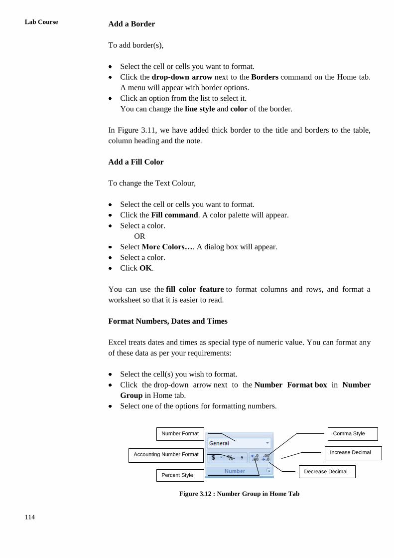
Format Numbers, Dates and Times
Excel treats dates and times as special type of numeric value. You can format any
of these data as per your requirements:
Select the cell(s) you wish to format.
Click the drop-down arrow next to the Number Format box in Number
Group in Home tab.
Select one of the options for formatting numbers.
Figure 3.12 : Number Group in Home Tab
Number Format
Accounting Number Format
Percent Style
Comma Style
Increase Decimal
Decrease Decimal
115
Spreadsheet By default, the numbers appear in the General category, which means there is no
special formatting.
In the Number group, you have some other options. For example, you can change
the another currency format, set numbers to percents, add commas, and change
the decimal location.
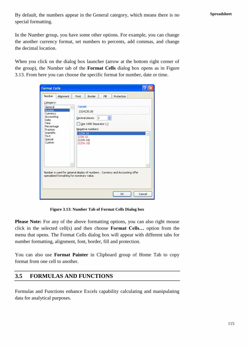
When you click on the dialog box launcher (arrow at the bottom right corner of
the group), the Number tab of the Format Cells dialog box opens as in Figure
3.13. From here you can choose the specific format for number, date or time.
Figure 3.13: Number Tab of Format Cells Dialog box
Please Note: For any of the above formatting options, you can also right mouse
click in the selected cell(s) and then choose Format Cells… option from the
menu that opens. The Format Cells dialog box will appear with different tabs for
number formatting, alignment, font, border, fill and protection.
You can also use Format Painter in Clipboard group of Home Tab to copy
format from one cell to another.
3.5 FORMULAS AND FUNCTIONS
Formulas and Functions enhance Excels capability calculating and manipulating
data for analytical purposes.
116
Lab Course
3.5.1 Formulas
A formula is a set of mathematical instructions that can be used to perform
calculations. Formulas are started in the formula box with an = sign. A Formula
may consist of:
Operators : Symbols (+, -, *, /, etc.) that specify the calculation to be
performed.
References : The cell or range of cells that you want to use in your
calculation.
Constants : Numbers or text values that do not change.
Functions : Predefined formulas in Excel.
3.5.1.1 Create a Simple Formula
We will learn to create a formula to add two numbers:
Click the cell where you want the formula to be defined (for example cell A3).
Type = sign to let Excel know that a formula is being defined.
Type the two numbers to be added with the operator. For example type
35+1330 in cell A3 (after = sign). Press Enter.
The result of the above addition operation is displayed in the cell A3, instead
of the formula that we had typed. If you select A3, the formula appears in the
formula bar.
We can now modify the above formula to add contents of two cells instead of the
constant values:
Click the cell where you want the formula to be defined and the answer will
appear (for example cell A3).
Type = sign to let Excel know that a formula is being defined.
Type the cell number (example A1) that contains the first number to be added.
Then type + operator and then the cell number (example A3) that contains the
second number to be added. For example type A1+A3 in cell A3 (after =
sign). Please note, if a cell does not contain a number then it is treated as
containing zero.
Press Enter.
The result of the above addition operation is displayed in the cell A3. Cell A3
will display the value 333.
Change the value in cell A1 to 300, and notice that the value in cell A3
automatically changes to 334.
3.5.1.2 Create a Simple Formula using Point and Click Method
To create a formula using mouse:
Click the cell where the answer will appear (B3, for example).
Type the equal sign (=).
117
Spreadsheet Click on the first cell to be included in the formula (B1, for example).
Type the operator sign (+ for addition or – for subtraction or * for
multiplication or / for division) .
Click on the next cell in the formula (B3, for example).
Press Enter or click Enter button on the formula bar.
3.5.2 Using Cell References
When a cell address is used as part of a formula, it is called a cell reference
because instead of entering specific numbers into a formula, the cell address
referring to a specific cell is being used.
You have used Fill Handle in the auto fill feature in section 3.4.7. The same
feature can be used to copy formulas from one cell to another. For example, if you
have the formula =A1+B1 in cell C1, and you can use the fill handle to fill the
formula into cell C3. Note that the formula won’t appear the same in C3 as it does
in C1. Instead of =A1+B1, you will see =A3+B3 in cell C3. This is called
Relative Reference where cell references in formulas has changed cell addresses
relative to the row and column they are moved to. In relative reference, formulas
automatically adjust to new locations when they are pasted into different cells.
Sometimes, our requirement is such that we don’t want this change of cell address
on pasting. To achieve this, cells must be addressed by Absolute Reference.
In Absolute cell references, a formula always refers to the same cell or cell
range used in it. If a formula is copied to a different location, then the cell address
remains the same. An absolute reference is designated in the formula by the
addition of a dollar sign ($). It can precede the column reference or the row
reference, or both. Examples of absolute referencing are:
$A1 - here the column will not change when copied.
A$1 – here the row will not change when copied.
$A$1 – here both row and column will not change when copied.
In the above example, if we have formula as =$A$1+$B$1 in cell C1 and we copy
this formula in cell C3, then you will still see =$A$1+$B$1 in cell C3.
3.5.3 Linking Worksheets
Sometimes, you may want to use the value from a cell in another worksheet
within the same workbook in a formula. For example, the value of cell A1 in the
current worksheet and cell A3 in the second worksheet can be added using the
format "sheetname!celladdress". The formula for this example would be
"=A1+Sheet3!A3" where the value of cell A1 in the current worksheet is added to
the value of cell A3 in the worksheet named "Sheet3".
118
Lab Course
3.5.4 Functions
A function is a built in pre defined formula in Excel. One of the key benefits of
functions is that they save your time since you do not have to write the formula
yourself. For example, you could use an Excel function called Average to quickly
find the average of a range of numbers.
Excel has hundreds of different functions to assist with your calculations. Each
function has a particular syntax, which must be strictly followed for the function
to work correctly.
3.5.4.1 Function Library
The function library is a large group of functions on the Formula Tab of the
Ribbon. These functions include:
AutoSum: Easily calculates the sum of a range
Recently Used: All recently used functions
Financial: Accrued interest, cash flow return rates and additional financial
functions
Logical: And, If, True, False, etc.
Text: Text based functions
Date & Time: Functions calculated on date and time
Math & Trig: Mathematical Functions
You can visit each of these functions in the library to know more about them.
3.5.4.2 Insert a Function
To insert a function:
Click the cell where you want the function applied
Click the Insert Function button on the formula bar. The Insert Function
dialog box opens.
Choose the function from the dialog box. You may search on a particular
function in the dialog box or change the category and select the function. Help
for each function is available right there in the dialog box.
Click OK. Function Arguments dialog box opens.
Select the cells or range of cells for function arguments and click OK.
The Function is added to the formula bar
3.6 WORKING WITH WORKSHEETS
In this section we will learn to name, add, delete, group or ungroup worksheets.
We will also learn to format a worksheet for printing.
119
Spreadsheet 3.6.1 Name a Worksheet
The default names of Worksheets are Sheet1, Sheet3 and Sheet3. Since these
names are not useful and descriptive, we will learn to rename the worksheet.
You can rename a worksheet using any of the following ways:
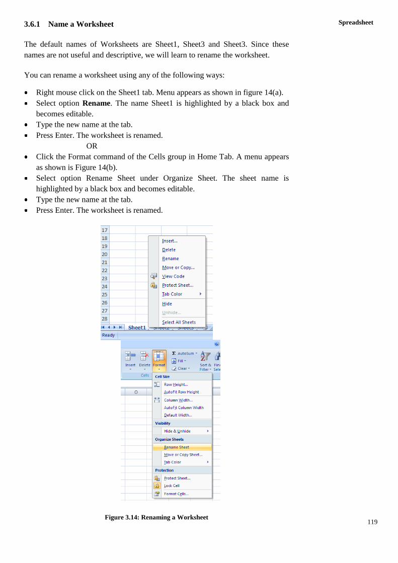
Right mouse click on the Sheet1 tab. Menu appears as shown in figure 14(a).
Select option Rename. The name Sheet1 is highlighted by a black box and
becomes editable.
Type the new name at the tab.
Press Enter. The worksheet is renamed.
OR
Click the Format command of the Cells group in Home Tab. A menu appears
as shown is Figure 14(b).
Select option Rename Sheet under Organize Sheet. The sheet name is
highlighted by a black box and becomes editable.
Type the new name at the tab.
Press Enter. The worksheet is renamed.
Figure 3.14: Renaming a Worksheet
120
Lab Course
3.6.2 Insert a New Worksheet
You can add worksheets to the workbook anytime you want. The new sheets
added will be named as Sheet4 and so on. There are many ways that you can add
a new worksheet:
Click on the Insert Worksheet icon near the worksheet tabs OR press
Shift+F11.
A new worksheet after the last tab will be added.
OR
Right mouse click on the worksheet tab.
Choose Insert… from the menu (shown in Figure 14(a)). Insert dialog box
opens.
Select Worksheet. Click Ok
A new worksheet before the selected tab will be added.
OR
Click the down arrow of Insert command in the Cells group of Home Tab. A
menu appears.
Choose Insert Sheet from the menu.
A new worksheet before the selected worksheet will be added.
3.6.3 Delete a Worksheet
Any number of worksheets can be deleted irrespective of the fact that they contain
any data or not. But, there should be at least one worksheet in the workbook. To
delete a worksheet:
Right mouse click on the worksheet tab.
Choose Delete from the menu (shown in Figure 14(a)).
The selected worksheet is deleted.
OR
Click the down arrow of Delete command in the Cells group of Home Tab. A
menu appears.
Choose Delete Sheet from the menu.
The selected worksheet is deleted.
3.6.4 Grouping Worksheets
If the multiple worksheets of a workbook contain identical formula and
formatting, then you can group them together. When the worksheets are grouped
together, then any change made to one worksheet will be applied to all other
worksheets in the group. You can group both contiguous and noncontiguous
worksheets. To group contiguous worksheets:
Click on the first worksheet tab.
Press the Shift key.
121
Spreadsheet While holding the Shift key, click the last worksheet tab you want in the
group.
Release the Shift key.
All the sheets from the first sheet to the last sheet are now grouped. The tab
colour will now change to white indicating that they are grouped together.
To group noncontiguous worksheets:
Click on the first worksheet tab.
Press the Ctrl key.
While holding the Ctrl key, select all the other worksheets you want in the
group.
Release the Ctrl key.
All the sheets that you selected while keeping the Ctrl key pressed would be
grouped together and sheet tabs will appear white.
3.6.5 Ungrouping Worksheets
To ungroup worksheets:
Right mouse click one of the worksheets in the group.
Select Ungroup Sheets from the menu.
3.6.6 Reposition Worksheets in a Workbook
To change the position of worksheets in a workbook:
Click and hold the worksheet tab that is to moved until an arrow appears on
the left corner of the sheet.
Drag the worksheet to the desired location
3.6.7 Hide Worksheets
To hide a worksheet:
Right-click on the tab of the sheet you wish to hide.
Select Hide
OR
Click Format button.
Select Hide & Unhide under Visibility in the menu.
Choose Hide Sheet option.
To unhide a worksheet:
Right-click on tab of any sheet.
122
Lab Course
Select Unhide…. A dialog box with the list of hidden worksheets is
displayed.
Choose the sheet to unhide.
OR
Click Format button.
Select Hide & Unhide under Visibility in the menu.
Choose Unhide Sheet… option. A dialog box with the list of hidden
worksheets is displayed.
Choose the sheet to unhide.
3.6.8 Formatting and Printing the Workbook
In this section, we will learn how to set page headers, footers, margin, etc and
prepare our workbook for printing.
To Change Page Orientation
Select Page Layout Tab on the Ribbon.
Click Orientation command in the Page Setup group.
Choose the orientation you want – Landscape (horizontal) or Portrait
(vertical).
To Change Paper Size
Select Page Layout Tab on the Ribbon.
Click Size command in the Page Setup group.
A drop down menu appears with all the available paper sizes. Current size is
highlighted.
Choose the size option. Page size of workbook changes.
To Set Page Margins
Select Page Layout Tab on the Ribbon.
Click Margins command in the Page Setup group.
Choose the predefined margins from the list.
OR
Customize your margins by selecting Custom Margins from the menu and
entering the desired margins in the appropriate fields.
To Set Headers and Footers
The header is the text that appears in the top margin of every page of the printed
worksheet. Similarly, the footer is the text that appears in the bottom margin of
every page of the printed worksheet. To add header and footer:
Select Insert Tab on the Ribbon.
123
Spreadsheet Click the Header & Footer button in the Text group. A Design context tab
appears under Header & Footer Tools. And worksheet changes to Page Layout
view from the Normal view. Page Layout view structures the worksheet so
that it is easy to change the format of the worksheet.
Both Header and Footer are divided into three sections: left, center, right. You
can type in your custom header/ footer or you can use predefined headers and
footers. Click on Header/ Footer button in Header & Footer group of Design
context tab to see the list of pre-defined headers and footers.
To Use Scale to Fit
Scale to Fit is a useful feature that can help you format spreadsheets to fit on a
page.
Select the Page Layout tab.
Locate the Scale to Fit group.
Enter a specific height and width, or use the percentage field to decrease the
spreadsheet by a specific percent.
Be careful with how small you scale the information – you should be able to read
it.
To Define a Print Area
At times you may want to print just a part of the whole worksheet. In that case
you need to select your print area that you need to be printed. To define your print
area:
Click and drag your mouse to select the cells you wish to print.
Click the Print Area command in Page Setup group of Page Layout Tab.
Choose Set Print Area. Now, only the selected cells will print. You can
confirm this by viewing the spreadsheet in Print Preview.
To return to printing entire worksheet, which is the default setting, click the Print
Area command and select Clear Print Area.
To Print Titles on Each Page
Print Title command allows you to select specific rows and/or columns to
appear on each printed sheet. This helps when the worksheet prints into many
pages, since we can have row and column heading printed on each page for easy
association and readability.
Select the Page Layout tab.
Click the Print Titles command in Page Setup group. The Sheet tab of Page
Setup dialog box opens.
Click the icon at the end of the field Rows to repeat at top.
Select the row headings in the spreadsheet that you want to appear on each
printed page.
124
Lab Course
Repeat for the column, if required.
Click OK. The select row/ column will now appear on each printed page.
Preview before Printing
Click Office Button.
Select Print Print Preview. The worksheet opens in the Print Preview
mode. In Print Preview, you can access many of the same features that you
can from the Ribbon, through the Page Setup dialog box. However, in Print
Preview you can see how the spreadsheet will appear in printed format.
Click Print to print the document or Close Print Preview to come back to the
document in original mode.
You can modify page margins, orientation, page size, etc in Print Preview mode.
To Quick Print the Document
Click Office Button.
Select Print QuickPrint
The document prints to the default printer. It bypasses the Print dialog box.
To Print the Document
Click Office Button.
Select Print Print. The Print dialog box appears.
Select the printer from the drop down list.
Click Properties to change any necessary settings.
Select the pages you would like to print – specific pages, all of the worksheet,
a selected area, the active sheet, or the entire workbook.
Select the number of copies.
Click OK to print.
3.7 WORKING WITH TABLES AND CHARTS
Excel has features to help you manage and analyze related data. An Excel table
stores information in a consistent manner, making it easier to format, sort, and
filter worksheet data. Charts allow you to present information contained in the
worksheet in a graphic format, which makes information easy to analyze.
3.7.1 Tables
Typically, an Excel table has only column headings and no row headings. Once
you have converted the information into a table, you can sort and filter it as per
your requirements.
125
Spreadsheet 3.7.1.1 Create Table
To create a table you need to have information stored in columns:
Enter Column Headings for the table. Each heading should be in a different
cell in a row. Column headings are also known as field names. The column
headings should appear in a single row without any blank cells between the
entries.
Start adding data in the row right below column heading. This is the first
record/ row of the table.
Select any cell that contains the data.
Click on Format as Table button in the Styles group of Home tab. A gallery
of pre-defined styles of tables appears.
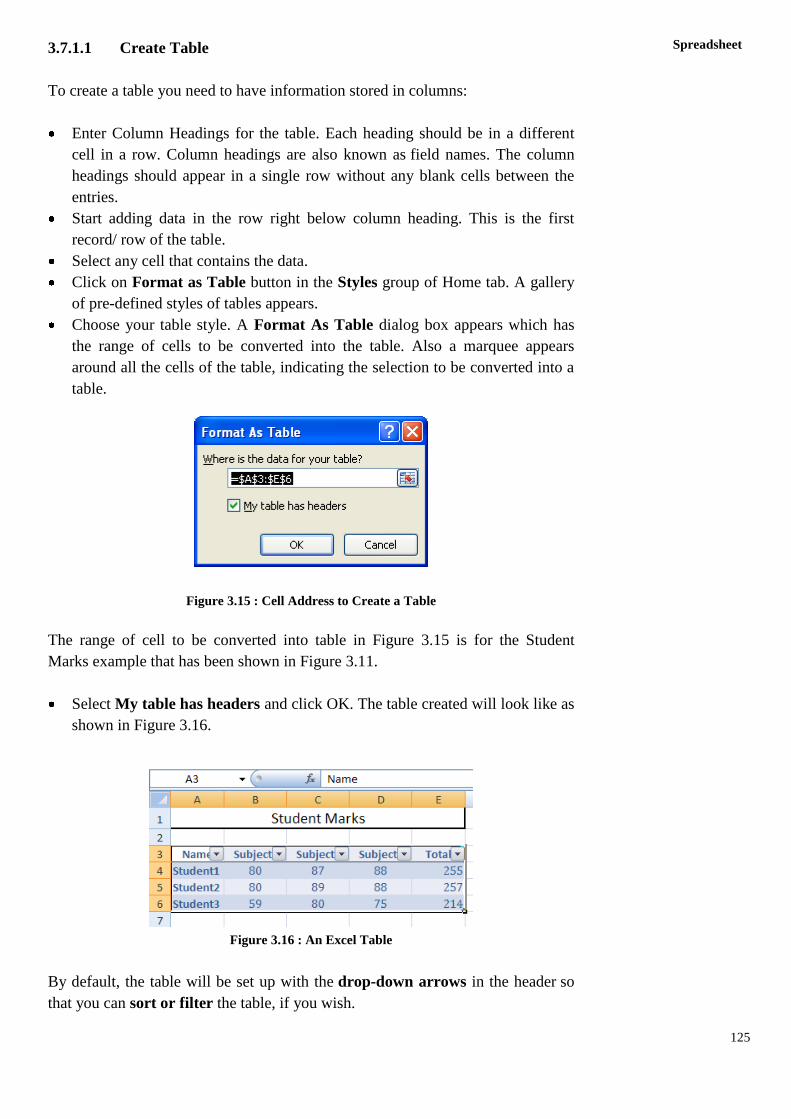
Choose your table style. A Format As Table dialog box appears which has
the range of cells to be converted into the table. Also a marquee appears
around all the cells of the table, indicating the selection to be converted into a
table.
Figure 3.15 : Cell Address to Create a Table
The range of cell to be converted into table in Figure 3.15 is for the Student
Marks example that has been shown in Figure 3.11.
Select My table has headers and click OK. The table created will look like as
shown in Figure 3.16.
Figure 3.16 : An Excel Table
By default, the table will be set up with the drop-down arrows in the header so
that you can sort or filter the table, if you wish.

126
Lab Course
Alternatively, after you have selected cell for table creation, you can also choose
the Table command button in the Tables group of the Insert tab. This opens
Create table dialog box with the range of cells to be converted into the table
(similar to as in Figure 3.15). When you click OK, the table is created in the
default style.
If you want to convert an existing Excel table back to a normal range of cells,
select any cell in the table and then click the Convert to Range button on the
Table Tools Design tab. All data and formatting is preserved. Using Table Tools
Design context tab, you can change table style, add or delete table rows, resize
table, remove duplicates, change table name and perform many more other
functions on the table.
3.7.1.2 Sort Data
Sorting allows you to reorder your data. To sort data:
Select a cell in the column you want to sort (for example, you can choose a
cell in Total column to sort on total in our Students Marks example).
Click the Sort & Filter command in the Editing group on the Home tab.
In the menu you can choose Smallest to Largest or Largest to Smallest
order for sort.
For multi level sorting, you can also choose Custom Sort… and specify
different columns and the order of sort for each in the dialog box.
Alternatively, you can also choose sort options from the Sort & Filter group in
the Data Tab.
3.7.1.3 Filter Data
Filtering allows you to display only data that meets certain criteria. To filter:
Click the column or columns that contain the data you wish to filter.
On the Home tab, click on Filter button in the Sort & Filter group. Drop
down arrows appear on column headings. These arrows would already be
there if you are using an Excel table.
Click the arrow in the column heading.
Choose the appropriate data value(s) to filter from the drop down menu.
To clear the Filter, click the Sort & Filter button and choose Filter again.

127
Spreadsheet 3.7.2 Charts
Charts allow you to present information contained in the worksheet in a graphic
format. Excel offers many types of charts including: Column, Line, Pie, Bar,
Area, Scatter and more. To create a chart we first need to have the data.
3.7.2.1 Add Data
We will use the following sample data in our example. We will create a graph to
compare daily attendance of two classes.
Figure 3.17: Sample Data for creating Graph
This is the source data for our chart, since it will be based on this data. Any
change in the source data will automatically be reflected in the chart.
3.7.2.2 Create Chart
Select the cells that that contain the data you want to use in the chart,
including the column titles and the row labels.
Click the Insert tab on the Ribbon.
Click on one of the chart options from the Chart group. In this example, we
will use the Columns option.
Select a type of chart you want to create from the list. For our example, we
will use a 3-D Clustered Column. The chart appears in the worksheet. Also
notice Design, Layout and Format context tabs under Chart Tools:
Design Tab: has commands to control the chart type, layout, styles, and location
of the chart.
Layout Tab: has commands to control pictures insert, shapes and text boxes,
labels, axes, background, and analysis.
Format Tab: has commands to modify shape styles, word styles and size of the
chart.
128
Lab Course
3.7.2.3 Apply Layout
To apply the layout:
Click your chart. The Chart Tools become available.
Choose the Design tab.
Click the Quick Layout button in the Chart Layout group. A list of chart
layouts appears.
Select the layout. Excel applies the layout to your chart. We have chose layout
9 for our example.
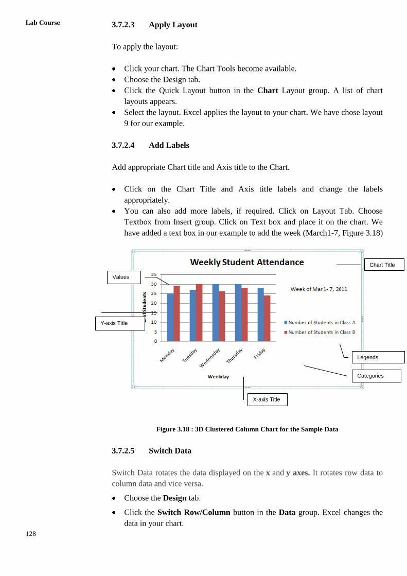
3.7.2.4 Add Labels
Add appropriate Chart title and Axis title to the Chart.
Click on the Chart Title and Axis title labels and change the labels
appropriately.
You can also add more labels, if required. Click on Layout Tab. Choose
Textbox from Insert group. Click on Text box and place it on the chart. We
have added a text box in our example to add the week (March1-7, Figure 3.18)
Figure 3.18 : 3D Clustered Column Chart for the Sample Data
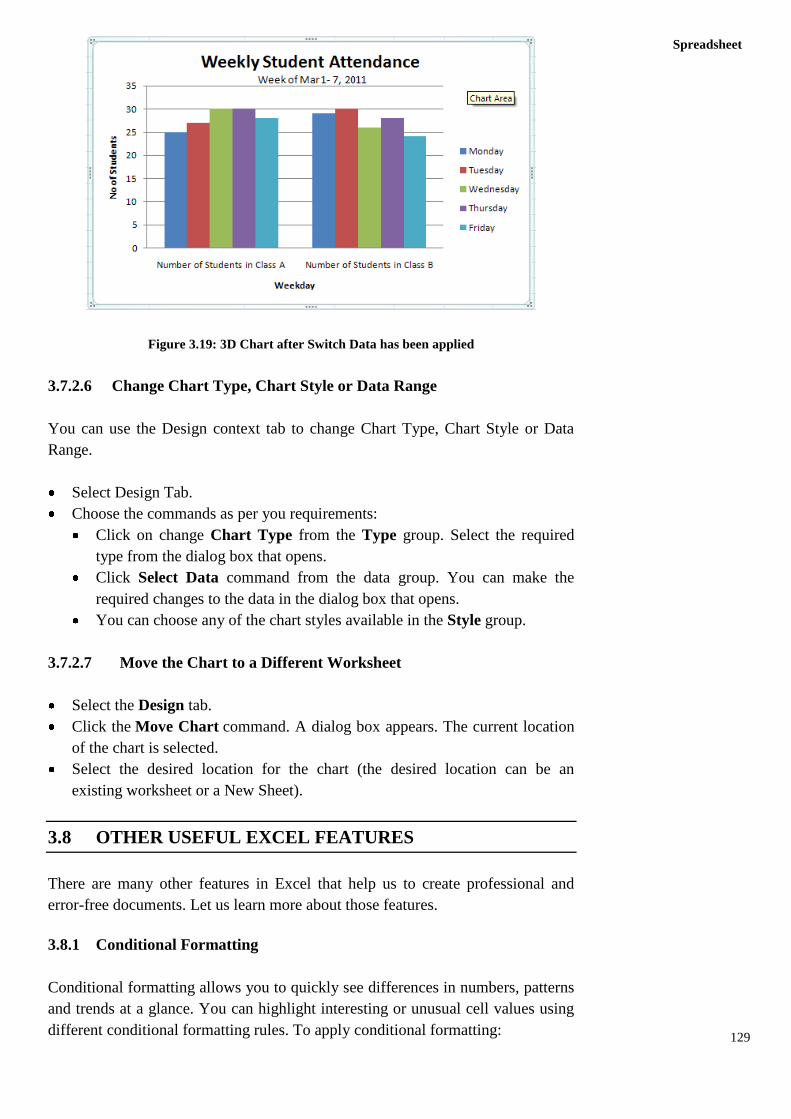
3.7.2.5 Switch Data
Switch Data rotates the data displayed on the x and y axes. It rotates row data to
column data and vice versa.
Choose the Design tab.
Click the Switch Row/Column button in the Data group. Excel changes the
data in your chart.
Chart Title
Y-axis Title
X-axis Title
Legends
Categories
Values
129
Spreadsheet
Figure 3.19: 3D Chart after Switch Data has been applied
3.7.2.6 Change Chart Type, Chart Style or Data Range
You can use the Design context tab to change Chart Type, Chart Style or Data
Range.
Select Design Tab.
Choose the commands as per you requirements:
Click on change Chart Type from the Type group. Select the required
type from the dialog box that opens.
Click Select Data command from the data group. You can make the
required changes to the data in the dialog box that opens.
You can choose any of the chart styles available in the Style group.
3.7.2.7 Move the Chart to a Different Worksheet
Select the Design tab.
Click the Move Chart command. A dialog box appears. The current location
of the chart is selected.
Select the desired location for the chart (the desired location can be an
existing worksheet or a New Sheet).
3.8 OTHER USEFUL EXCEL FEATURES
There are many other features in Excel that help us to create professional and
error-free documents. Let us learn more about those features.
3.8.1 Conditional Formatting
Conditional formatting allows you to quickly see differences in numbers, patterns
and trends at a glance. You can highlight interesting or unusual cell values using
different conditional formatting rules. To apply conditional formatting:
130
Lab Course
Select the cells you wish to format.
Select the Home tab and locate the Styles group.
Click the Conditional Formatting command. A menu will appear with your
formatting options. You can choose from the predefined rules or create your
own new rule.
Select one of the options to apply it to the selected cells. When you choose a
predefined rule, a cascading menu will appear. And an additional dialog box
may appear, depending on the option you choose. Make the necessary choices,
and click OK.
To Remove Conditional Formatting Rules:
Click the Conditional Formatting command.
Select Clear Rules. A cascading menu appears.
Choose to clear rules from the entire worksheet or the selected cells.
3.8.2 Freeze Rows and Columns
To freeze row(s) or column(s) mean that those row(s) or column(s) are always
visible on the screen and they never scroll. This feature is quite helpful while
working with very large worksheets, where we want to see certain rows/ columns
all the time (for example labels or headings) to be able to relate and analyze data.
To freeze row or column:
Select the row below the one you want to freeze and select the column right of
one you want to freeze. For example, if you want to freeze row 3, then select
row 3 and if you want to freeze column B, then choose column C. If you want
to freeze both row and column, then choose the correct cell.
Click on View tab on the Ribbon.
Click in Freeze Panes Command in the Window group.
Select Freeze Panes from the menu.
A thin black line appears below the frozen row and right of frozen column.
To unfreeze the panes, select Unfreeze Panes option from the menu that appears
when you click Freeze Panes command in the Window group of the View tab.
3.8.3 Find and Replace
To find data or find and replace data:
Click the Find & Select button on the Editing group of the Home tab.
Choose Find or Replace tab in the dialog box.
Complete the Find What text box.
Click on Options for more search options.
Use the button Replace All, Replace, Find All, Find Next as per the
requirements.
131
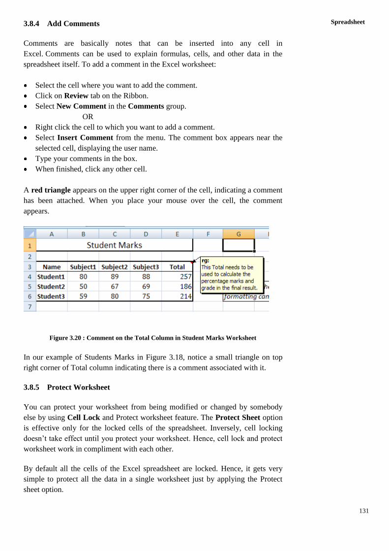
Spreadsheet 3.8.4 Add Comments
Comments are basically notes that can be inserted into any cell in
Excel. Comments can be used to explain formulas, cells, and other data in the
spreadsheet itself. To add a comment in the Excel worksheet:
Select the cell where you want to add the comment.
Click on Review tab on the Ribbon.
Select New Comment in the Comments group.
OR
Right click the cell to which you want to add a comment.
Select Insert Comment from the menu. The comment box appears near the
selected cell, displaying the user name.
Type your comments in the box.
When finished, click any other cell.
A red triangle appears on the upper right corner of the cell, indicating a comment
has been attached. When you place your mouse over the cell, the comment
appears.
Figure 3.20 : Comment on the Total Column in Student Marks Worksheet
In our example of Students Marks in Figure 3.18, notice a small triangle on top
right corner of Total column indicating there is a comment associated with it.
3.8.5 Protect Worksheet
You can protect your worksheet from being modified or changed by somebody
else by using Cell Lock and Protect worksheet feature. The Protect Sheet option
is effective only for the locked cells of the spreadsheet. Inversely, cell locking
doesn’t take effect until you protect your worksheet. Hence, cell lock and protect
worksheet work in compliment with each other.
By default all the cells of the Excel spreadsheet are locked. Hence, it gets very
simple to protect all the data in a single worksheet just by applying the Protect
sheet option.
132
Lab Course
Unlocking specific cells permits changes to be made to these cells after the
protect sheet option has been applied.
Unlock Cells
Cells in a worksheet are locked by default. We will unlock some of them:
Click on the Home tab.
Choose the Format option in Cells group to open the drop down list.
Click on Lock Cell option at the bottom of the list (under Protection).
The Lock Cell option works like an ON/OFF button. Since all cells are
initially locked in the worksheet, clicking on the option has the affect
of unlocking the highlighted cells. If you click on Lock Cell option again, it
will lock the selected cells.
Protect Worksheet
Once the cells have been locked, we will protect the worksheet:
Click on the Home tab.
Choose the Format option in Cells group to open the drop down list.
Click on Protect Sheet… option at the bottom of the list (under Protection) to
open the Protect Sheet dialog box.
Provide the password if you want to. Password does not prevent users from
opening and viewing the worksheet. Choose the other options according to
your requirements. Click OK.
Now you can access only unlocked cells on the worksheet.
3.8.6 Convert Text to Columns
Sometimes you might need to split data in one cell into two or more cells. For
example, when both first and last names in a worksheet are stored in one cell, but
they are required separately, then you can do this easily by utilizing the Convert
Text to Columns Wizard. Depending on your data, you can split the cell content
based on a delimiter, such as a space or a comma, or based on a specific column
break location within your data. To use this wizard:
Highlight the column in which you wish to split the data
Click the Text to Columns button in Data Tools group on the Data tab
Click Delimited if you have a comma or tab separating the data, or click fixed
widths to set the data separation at a specific size. Click Next.
In the next screen you either choose the delimiter (for delimited data) or
specify the location where to break the data (for fixed width data). Click Next.
In the next screen, specify data format and the destination columns for the
separated data. Click Finish. Data is separated.
133
Spreadsheet 3.9 SUMMARY
Spreadsheets enable working with data easy and effective. It has ability to store,
manipulate, format, sort, filter, retrieve, organize, represent and analyze data as
per your requirements.
You can save any kind of data, in any format in cells of a worksheet. Multiple
worksheets in a workbook enable you to store a large amount of data and manage
it efficiently. Formulas and Functions allow easy calculation and manipulation of
data. Tables facilitate uncomplicated organization and retrieval of data. Charts are
visual display of the information. Additionally, there are many formatting and
design features in the Excel program to create and print a professional looking
workbook.
A Spreadsheet program is useful is any kind of area, since it is associated with
data and information which is an important aspect of all of our lives. You can use
it for small purposes like maintaining birthday lists, home budgets or for big ones
like creating reports, preparing dashboards, for stock management, shipment
planning, as analytical tool in large corporate environments. A Spreadsheet
program can be used for any data related purpose.
3.10 LAB EXERCISE
1. Using ‘Excel Options’ do the following customizations:
a. Set default two worksheets in a workbook. Original number is three.
b. Disable autorecover for your current workbook.
c. Set the Recent number of documents to be displayed to two.
d. Don’t display grid lines.
e. Enable show page breaks.
f. Set the Enter key direction so that the cursor moves to right when you
press enter in a cell.
2. Open a new workbook. Create a table with two columns. Use columns A and
B of the worksheet. The headings for first one should be First Name. Give the
heading as Last Name for the second column. Add records in the table. Please
ensure that you enter all the data in the lower case. For example, you should
enter first name as rahul and second name as gandhi. Your data should
contain multiple records with the same first or last name. Save workbook as
Student.xlsx
3. Open Student.xlsx. Create another table using column E and F. Again the
heading would be First Name and Last Name. Using string functions, change
the names to proper case (for example to Rahul or Gandhi) and store in E and
F. Original data should remain. Save and Close the worksheet.
4. Open Student.xlsx. Hide Columns A and B. Rename Sheet1 as Student Name.
Delete all the worksheets in the workbook except Student Name. Add Borders
to the table. Format heading as: Bold, center aligned, increase font size,
change the font colour and the fill of the heading. Save and close.
134
Lab Course
5. Open Student.xlsx. Sort the records in alphabetical order of the first name.
Filter all records with last name Agarwal.
Now use a string function to concatenate the two names (first name and last
name) and store in the column D (give heading as Name).
6. Create a new workbook containing Student Marks. Add column headings :
Name, English, Hindi, Maths, Science, Social Science, Total Marks,
Percentage Marks. Add records to the table. You may copy name from
Student.xlsx. Add title to the table. Format the table properly. Use functions to
calculate Total Marks and Percentage. Freeze the panes, so that headings
don’t scroll. Add Headers and Footer to the worksheet. Preview the
worksheet. Save as StudentMarks.xlsx and close.
7. Create a table of records with columns Name and Donation Amount.
Donation amount should be formatted with two decimal places. There should
be at least twenty records in the table. Create a conditional format to highlight
top 3 donations with blue colour and lowest 3 donations with red colour. The
table should have a a heading.
8. Use Auto fill feature to fill column B with odd numbers and column C with
even numbers. There should be twenty records in each column. Save the
workbook as EvenOdd.xlsx
9. Using the workbook EvenOdd.xlsx, create a formula in column D1 to add B1
and C1. Copy the formula from D1 to all other following rows. Also use
formula to display the sum of all the values in column B in cell B35.
Similarly, for column C in cell C35. Add the label ‘Sum’ in cell A35. It
should be bold and double underlined. Save the workbook.
10. Open workbook EvenOdd.xlsx. Go to Sheet 3. Type the value 1.5 in cell A1.
Come back to Sheet1. Create a formula in E1 to multiply the value is D1 with
the value in cell A1of Sheet3. Copy the formula to other rows.
11. Create a table of expenses for a house hold. The table will have two column :
Expense name and Expense value in percent (it will the total percent spend
under this head). Create a Pie Chart for the same data. Examples of Expense
heads can be Food, education, utilities, clothing, house rent. The chart should
have proper Title, labels and legends.
12. Create a list of names with all the names in column A, stored in the format
Last name, First name, for example: Gandhi,Rahul. Use Convert to Text
feature to separate the first name and the last name. The original data should
not be lost.
3.11 FURTHER READINGS
Excel 3007 All-In-One Desk Reference for Dummies By Greg Harvey.
Teach Yourself Excel 3007 By Moira Stephen.
Microsoft Excel 3007 for Dummies By Greg Harvey.
http://www.gcflearnfree.org/excel3007.