Unit 39: Further Mathematics Unit Workbook 2...Unit WorkBook 2 – Level 5 ENG – U39 Further Mathematics– LO2 Matrix Methods © 2018 UniCourse Ltd. All Rights Reserved. Page 5

Unit WorkBook 2 – Level 5 ENG – U39 Further Mathematics– LO2 Matrix Methods

© 2018 UniCourse Ltd. All Rights Reserved.

Page 1 of 25

Pearson BTEC Levels 5 Higher Nationals in Engineering (RQF)

Unit 39: Further Mathematics

Unit Workbook 2 in a series of 4 for this unit

Learning Outcome 2

Matrix Methods

Sample



Page 4 of 25

2.1 Vector Notation and Operations

2.1.1 Cartesian Co-Ordinates and Unit Vectors A Scalar is a quantity with magnitude only. Examples of a scalar are an amount of cash or the age of a

person. A Vector has both magnitude and direction. Examples of a vector are the motion of a car or the

magnetic field emanating from a bar magnet.

We shall initially examine vectors in two dimensions (north-south and east-west if you like) and then move

on to look at vectors in three dimensions (perhaps inside a cube).

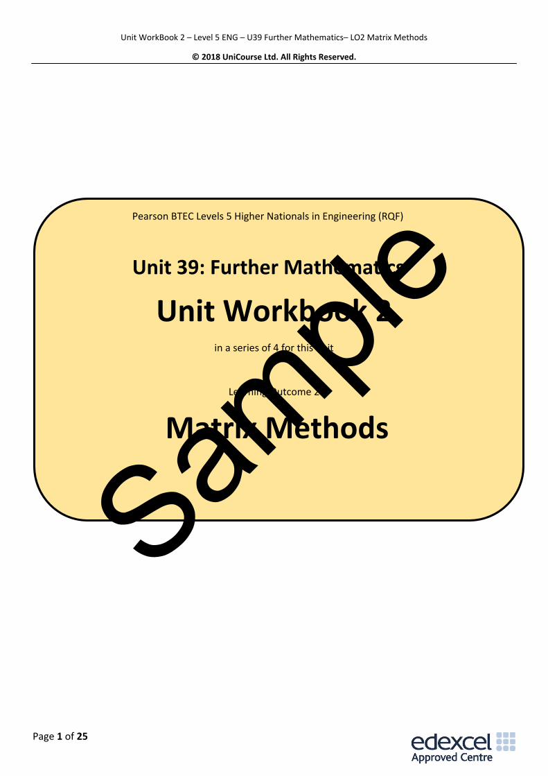
Let’s look at the Cartesian co-ordinate system…

The point in red sits in a Cartesian co-ordinate system. It has a horizontal component (𝑥 = 4) and a vertical

component (𝑦 = 3). We may represent the same point as a vector (in blue). A little bit of Pythagoras will

yield a length of 5 for this vector and an angle of 36.8o from the horizontal reference plane. Should a car be

travelling at 5 mph in a direction 4 miles due east and 3 miles due north then it may be represented as per

the figure on the right i.e. a vector quantity.

A Unit Vector is a scaled version of a vector, always having a magnitude (length) of 1. To find the unit

vector version of a starting vector we simply divide the vector by its original magnitude. In our example

above, the magnitude is 5 so we divide 5 to give a unit vector magnitude of 1. The horizontal component of

this unit vector will then be 4/5 = 0.8 and the vertical component will be 3/5 = 0.6. A quick check using

Pythagoras will give magnitude = sqrt(0.82 + 0.62) = 1. Unit vectors will be very useful in our calculations,

especially when we work in three dimensions. Let’s look at a unit vector co-ordinate systems in two and

three dimensions…

Sample



Page 5 of 25

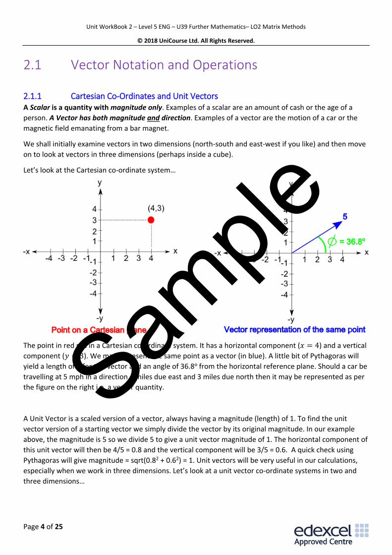
The 2-D drawing shows our normal x and y axes in black. If we take a vector along the x axis and give it a

length of 1 then this will be a unit vector along x which is called 𝑖̂. Along the y axis we may produce a unit

vector called 𝑗̂. The blue vector has a horizontal component of 2𝑖̂ and a vertical component of 1𝑗̂ or, just 𝑗̂,

to save some ink. The 3-D drawing on the right shows these unit vectors again, plus another one (�̂�) to

represent the third dimension. These unit vectors will be extensively used throughout this workbook and in

your third assignment.

2.1.2 Types of Vector and Vector Representation There are many types of vector. Some of the most notable ones are…

▪ Co-initial vectors their starting points are the same

▪ Co-terminal vectors their ending points are all the same

▪ Coplanar vectors they lie in the same plane

▪ Null vector has direction but no magnitude (advanced stuff)

▪ Unit vectors we now know a bit about these

▪ Resultant vector result of adding two vectors together

▪ Like vectors they act in the same direction

▪ Unlike vectors they are parallel but act in opposite directions

▪ Axial vectors act along one of the axes

▪ Space vector exists within 3-D space

Representation of vectors is performed by using multiples of the unit vector along each axis. The previous

sketch represented a vector in this way.

Sample



Page 6 of 25

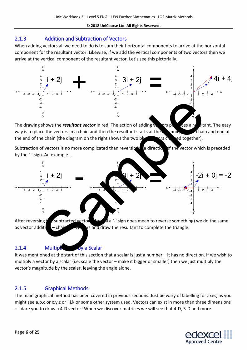
2.1.3 Addition and Subtraction of Vectors When adding vectors all we need to do is to sum their horizontal components to arrive at the horizontal

component for the resultant vector. Likewise, if we add the vertical components of two vectors then we

arrive at the vertical component of the resultant vector. Let’s see this pictorially…

The drawing shows the resultant vector in red. The action of adding vectors produces a resultant. The easy

way is to place the vectors in a chain and then the resultant starts at the beginning of the chain and end at

the end of the chain (the diagram on the right shows the two blue vectors chained together).

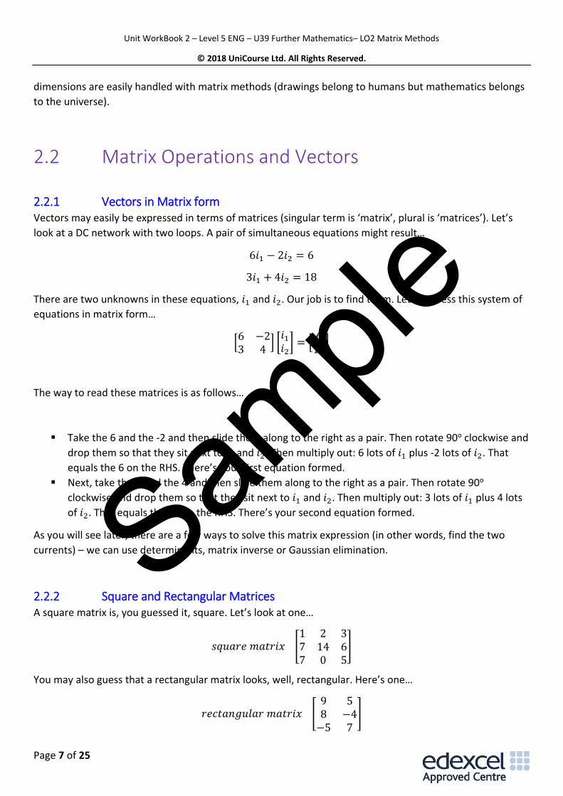
Subtraction of vectors is no more complicated than reversing the direction of the vector which is preceded

by the ‘-‘ sign. An example…

After reversing the subtracted vector (after all a ‘-‘ sign does mean to reverse something) we do the same

as vector addition – chain the vectors and draw the resultant to complete the triangle.

2.1.4 Multiplication by a Scalar It was mentioned at the start of this section that a scalar is just a number – it has no direction. If we wish to

multiply a vector by a scalar (i.e. scale the vector – make it bigger or smaller) then we just multiply the

vector’s magnitude by the scalar, leaving the angle alone.

2.1.5 Graphical Methods The main graphical method has been covered in previous sections. Just be wary of labelling for axes, as you

might see a,b,c or x,y,z or i,j,k or some other system used. Vectors can exist in more than three dimensions

– I dare you to draw a 4-D vector! When we discover matrices we will see that 4-D, 5-D and more

Sample



Page 7 of 25

dimensions are easily handled with matrix methods (drawings belong to humans but mathematics belongs

to the universe).

2.2 Matrix Operations and Vectors

2.2.1 Vectors in Matrix form Vectors may easily be expressed in terms of matrices (singular term is ‘matrix’, plural is ‘matrices’). Let’s

look at a DC network with two loops. A pair of simultaneous equations might result…

6𝑖1 − 2𝑖2 = 6

3𝑖1 + 4𝑖2 = 18

There are two unknowns in these equations, 𝑖1 and 𝑖2. Our job is to find them. Let’s express this system of

equations in matrix form…

[6 −23 4

] [𝑖1

𝑖2] = [

618

]

The way to read these matrices is as follows…

▪ Take the 6 and the -2 and then slide them along to the right as a pair. Then rotate 90o clockwise and

drop them so that they sit next to 𝑖1 and 𝑖2. Then multiply out: 6 lots of 𝑖1 plus -2 lots of 𝑖2. That

equals the 6 on the RHS. There’s your first equation formed.

▪ Next, take the 3 and the 4 and then slide them along to the right as a pair. Then rotate 90o

clockwise and drop them so that they sit next to 𝑖1 and 𝑖2. Then multiply out: 3 lots of 𝑖1 plus 4 lots

of 𝑖2. That equals the 18 on the RHS. There’s your second equation formed.

As you will see later, there are a few ways to solve this matrix expression (in other words, find the two

currents) – we can use determinants, matrix inverse or Gaussian elimination.

2.2.2 Square and Rectangular Matrices A square matrix is, you guessed it, square. Let’s look at one…

𝑠𝑞𝑢𝑎𝑟𝑒 𝑚𝑎𝑡𝑟𝑖𝑥 [1 2 37 14 67 0 5

]

You may also guess that a rectangular matrix looks, well, rectangular. Here’s one…

𝑟𝑒𝑐𝑡𝑎𝑛𝑔𝑢𝑙𝑎𝑟 𝑚𝑎𝑡𝑟𝑖𝑥 [9 58 −4

−5 7]

Sample



Page 8 of 25

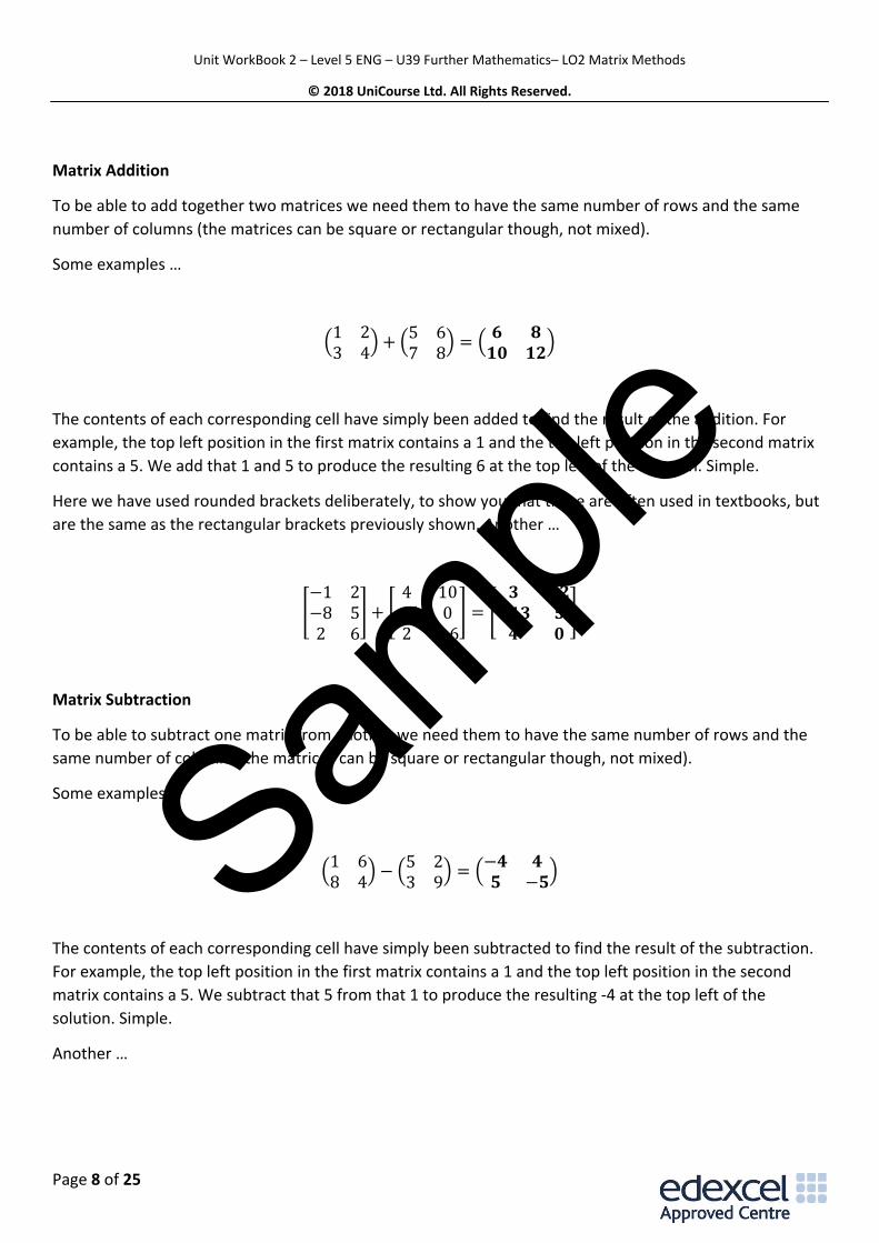
Matrix Addition

To be able to add together two matrices we need them to have the same number of rows and the same

number of columns (the matrices can be square or rectangular though, not mixed).

Some examples …

(1 23 4

) + (5 67 8

) = (𝟔 𝟖

𝟏𝟎 𝟏𝟐)

The contents of each corresponding cell have simply been added to find the result of the addition. For

example, the top left position in the first matrix contains a 1 and the top left position in the second matrix

contains a 5. We add that 1 and 5 to produce the resulting 6 at the top left of the solution. Simple.

Here we have used rounded brackets deliberately, to show you that these are often used in textbooks, but

are the same as the rectangular brackets previously shown. Another …

[−1 2−8 52 6

] + [4 10

−5 02 −6

] = [𝟑 𝟏𝟐

−𝟏𝟑 𝟓𝟒 𝟎

]

Matrix Subtraction

To be able to subtract one matrix from another we need them to have the same number of rows and the

same number of columns (the matrices can be square or rectangular though, not mixed).

Some examples …

(1 68 4

) − (5 23 9

) = (−𝟒 𝟒𝟓 −𝟓

)

The contents of each corresponding cell have simply been subtracted to find the result of the subtraction.

For example, the top left position in the first matrix contains a 1 and the top left position in the second

matrix contains a 5. We subtract that 5 from that 1 to produce the resulting -4 at the top left of the

solution. Simple.

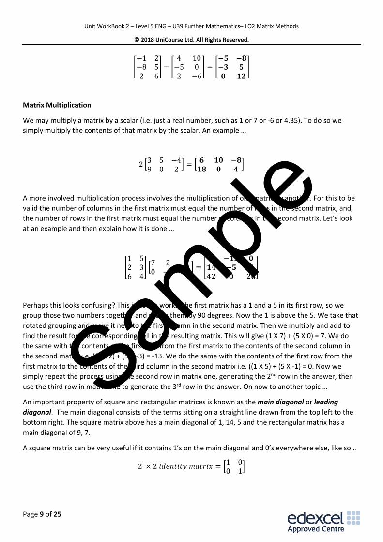
Another …

Sample



Page 9 of 25

[−1 2−8 52 6

] − [4 10

−5 02 −6

] = [−𝟓 −𝟖−𝟑 𝟓𝟎 𝟏𝟐

]

Matrix Multiplication

We may multiply a matrix by a scalar (i.e. just a real number, such as 1 or 7 or -6 or 4.35). To do so we

simply multiply the contents of that matrix by the scalar. An example …

2 [3 5 −49 0 2

] = [𝟔 𝟏𝟎 −𝟖

𝟏𝟖 𝟎 𝟒]

A more involved multiplication process involves the multiplication of one matrix by another. For this to be

valid the number of columns in the first matrix must equal the number of rows in the second matrix, and,

the number of rows in the first matrix must equal the number of columns in the second matrix. Let’s look

at an example and then explain how it is done …

[1 52 36 4

] [7 2 50 −3 −1

] = [𝟕 −𝟏𝟑 𝟎

𝟏𝟒 −𝟓 𝟕𝟒𝟐 𝟎 𝟐𝟔

]

Perhaps this looks confusing? This is how it works; the first matrix has a 1 and a 5 in its first row, so we

group those two numbers together and rotate them by 90 degrees. Now the 1 is above the 5. We take that

rotated grouping and move it next to the first column in the second matrix. Then we multiply and add to

find the result for the corresponding cell in the resulting matrix. This will give (1 X 7) + (5 X 0) = 7. We do

the same with the contents of the first row from the first matrix to the contents of the second column in

the second matrix i.e. ((1 X 2) + (5 X -3) = -13. We do the same with the contents of the first row from the

first matrix to the contents of the third column in the second matrix i.e. ((1 X 5) + (5 X -1) = 0. Now we

simply repeat the process using the second row in matrix one, generating the 2nd row in the answer, then

use the third row in matrix one to generate the 3rd row in the answer. On now to another topic …

An important property of square and rectangular matrices is known as the main diagonal or leading

diagonal. The main diagonal consists of the terms sitting on a straight line drawn from the top left to the

bottom right. The square matrix above has a main diagonal of 1, 14, 5 and the rectangular matrix has a

main diagonal of 9, 7.

A square matrix can be very useful if it contains 1’s on the main diagonal and 0’s everywhere else, like so…

2 × 2 𝑖𝑑𝑒𝑛𝑡𝑖𝑡𝑦 𝑚𝑎𝑡𝑟𝑖𝑥 = [1 00 1

]

Sample



Page 10 of 25

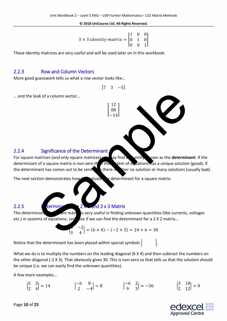
3 × 3 𝑖𝑑𝑒𝑛𝑡𝑖𝑡𝑦 𝑚𝑎𝑡𝑟𝑖𝑥 = [1 0 00 1 00 0 1

]

These identity matrices are very useful and will be used later on in this workbook.

2.2.3 Row and Column Vectors More good guesswork tells us what a row vector looks like…

[7 3 −5]

… and the look of a column vector…

[1288

−14]

2.2.4 Significance of the Determinant For square matrices (and only square matrices) we may find a quantity known as the determinant. If the

determinant of a square matrix is non-zero then the system of equations has a unique solution (good). If

the determinant has comes out to be zero then there is either no solution or many solutions (usually bad).

The next section demonstrates how to evaluate the determinant for a square matrix.

2.2.5 Determinant for a 2 x 2 and 3 x 3 Matrix The determinant of a square matrix is very useful in finding unknown quantities (like currents, voltages

etc.) in systems of equations. Let’s see if we can find the determinant for a 2 X 2 matrix…

|6 −23 4

| = (6 × 4) − (−2 × 3) = 24 + 6 = 30

Notice that the determinant has been placed within special symbols | |.

What we do is to multiply the numbers on the leading diagonal (6 X 4) and then subtract the numbers on

the other diagonal (-2 X 3). That obviously gives 30. This is non-zero so that tells us that the solution should

be unique (i.e. we can easily find the unknown quantities).

A few more examples…

|5 32 4

| = 14 |−6 82 −4

| = 8 |−6 29 3

| = −36 |3 182 12

| = 0

Sample



Page 11 of 25

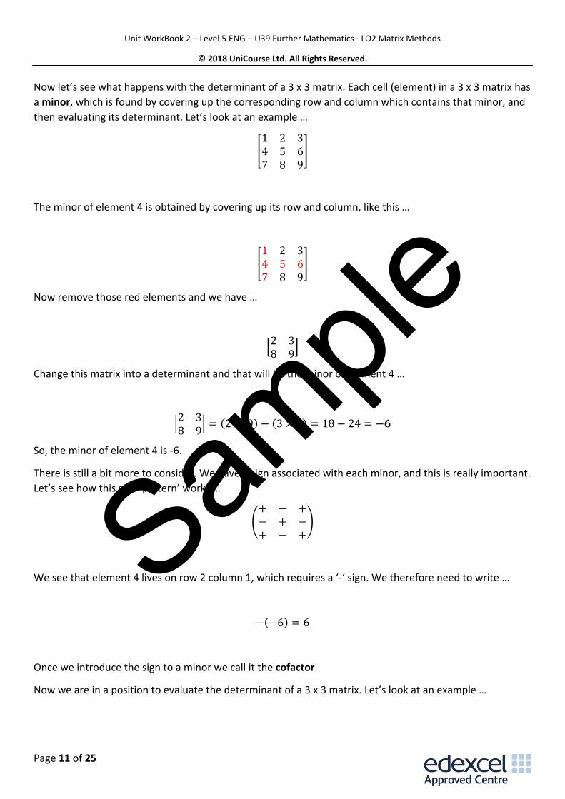
Now let’s see what happens with the determinant of a 3 x 3 matrix. Each cell (element) in a 3 x 3 matrix has

a minor, which is found by covering up the corresponding row and column which contains that minor, and

then evaluating its determinant. Let’s look at an example …

[1 2 34 5 67 8 9

]

The minor of element 4 is obtained by covering up its row and column, like this …

[1 2 34 5 67 8 9

]

Now remove those red elements and we have …

[2 38 9

]

Change this matrix into a determinant and that will be the minor of element 4 …

|2 38 9

| = (2 × 9) − (3 × 8) = 18 − 24 = −𝟔

So, the minor of element 4 is -6.

There is still a bit more to consider. We have a sign associated with each minor, and this is really important.

Let’s see how this sign ‘pattern’ works …

(+ − +− + −+ − +

)

We see that element 4 lives on row 2 column 1, which requires a ‘-‘ sign. We therefore need to write …

−(−6) = 6

Once we introduce the sign to a minor we call it the cofactor.

Now we are in a position to evaluate the determinant of a 3 x 3 matrix. Let’s look at an example …

Sample



Page 12 of 25

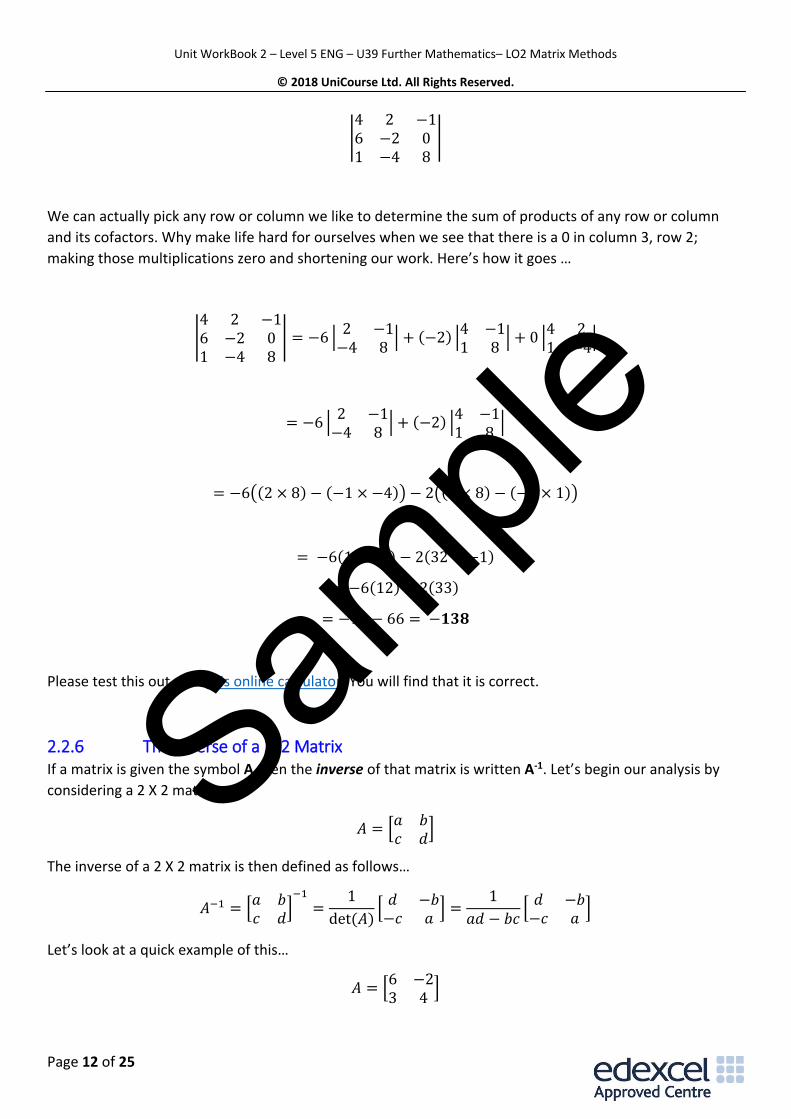
|4 2 −16 −2 01 −4 8

|

We can actually pick any row or column we like to determine the sum of products of any row or column

and its cofactors. Why make life hard for ourselves when we see that there is a 0 in column 3, row 2;

making those multiplications zero and shortening our work. Here’s how it goes …

|4 2 −16 −2 01 −4 8

| = −6 |2 −1

−4 8| + (−2) |

4 −11 8

| + 0 |4 21 −4

|

= −6 |2 −1

−4 8| + (−2) |

4 −11 8

|

= −6((2 × 8) − (−1 × −4)) − 2((4 × 8) − (−1 × 1))

= −6(16 − 4) − 2(32 − −1)

= −6(12) − 2(33)

= −72 − 66 = −𝟏𝟑𝟖

Please test this out with this online calculator. You will find that it is correct.

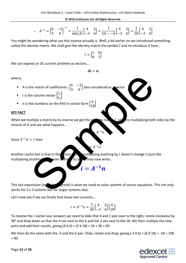
2.2.6 The Inverse of a 2x2 Matrix If a matrix is given the symbol A then the inverse of that matrix is written A-1. Let’s begin our analysis by

considering a 2 X 2 matrix…

𝐴 = [𝑎 𝑏𝑐 𝑑

]

The inverse of a 2 X 2 matrix is then defined as follows…

𝐴−1 = [𝑎 𝑏𝑐 𝑑

]−1

=1

det (𝐴)[

𝑑 −𝑏−𝑐 𝑎

] =1

𝑎𝑑 − 𝑏𝑐[

𝑑 −𝑏−𝑐 𝑎

]

Let’s look at a quick example of this…

𝐴 = [6 −23 4

]

Sample

https://matrixcalc.org/en/



Page 13 of 25

∴ 𝐴−1 = [6 −23 4

]−1

=1

det (𝐴)[

4 2−3 6

] =1

24 − −6[

4 2−3 6

] =1

30[

4 2−3 6

]

You might be wondering what use this inverse actually is. Well, a bit earlier on we introduced something

called the identity matrix. We shall give the identity matrix the symbol 𝐼 and re-introduce it here…

𝐼 = [1 00 1

]

We can express or DC current problem as vectors…

𝑨𝒊 = 𝒏

where;

▪ A is the matrix of coefficients…[6 −23 4

] also considered as a vector

▪ 𝑖 is the column vector [𝑖1

𝑖2]

▪ 𝑛 is the numbers on the RHS in vector form [6

18]

KEY FACT

When we multiply a matrix by its inverse we get the identity matrix 𝐼. Let’s try multiplying both sides by the

inverse of A and see what happens…

𝐴−1𝐴𝑖 = 𝐴−1𝑛

Since 𝐴−1𝐴 = 𝐼 then

𝐼𝑖 = 𝐴−1𝑛

Another useful fact is that in the vector world, multiplying anything by 𝐼 doesn’t change it (just like

multiplying anything by 1 never changes it) so we may now write...

𝒊 = 𝑨−𝟏𝒏

This last expression (much highlighted) is what we need to solve systems of vector equations. This not only

works for 2 x 2 systems but for larger systems also.

Let’s now see if we can finally find those two currents…

𝑖 = 𝐴−1𝑛 =1

30[

4 2−3 6

] [6

18]

To resolve the 𝑖 vector (our answer) we need to slide that 4 and 2 pair over to the right, rotate clockwise by

90o and drop down so that the 4 sits next to the 6 and the 2 sits next to the 18. We then multiply the new

pairs and add their results, giving (4 X 6) + (2 X 18) = 24 + 36 = 60.

We then do the same with the -3 and the 6 pair. Slide, rotate and drop, giving (-3 X 6) + (6 X 18) = -18 + 108

= 90.

Sample



Page 14 of 25

Our solution development now simplifies to…

𝑖 = 𝐴−1𝑛 =1

30[6090

]

We mentioned earlier that multiplying a scalar by a vector simply means multiplying the scalar by the

magnitude, so the 60 must be multiplied by 1/30 giving 2 and the 90 must also be multiplied by 1/30 giving

3. Finally, we arrive at our answer…

𝑖 = [𝑖1

𝑖2] = [

23

]

That’s a vector way of saying that current 𝒊𝟏 is 2 Amps and current 𝒊𝟐 is 3 Amps.

2.2.7 Gaussian Elimination for 2 X 2 Systems This is a quick method to find the unknowns in a set of simultaneous equations. Given two simultaneous

equations…

𝑎11𝑥 + 𝑎12𝑦 = 𝑏1

𝑎21𝑥 + 𝑎22𝑦 = 𝑏2

NOTE: the first subscript refers to the row number and the second subscript refers to the column number.

We’d like to find those 𝑥 and 𝑦 terms, which are just mere numbers. The approach is to try to eliminate the

lower left term completely so that we may then easily see the value of 𝑦. Once that is known then we use

back substitution to find 𝑥. This is best explained with an example…

6𝑖1 − 2𝑖2 = 6

3𝑖1 + 4𝑖2 = 18

We’d like to eliminate the lower left term – how can we do that? Well, what if we multiply the top

equation by -0.5? That will then give us the pair of equations…

−3𝑖1 + 𝑖2 = −3

3𝑖1 + 4𝑖2 = 18

If we now add these equations (like for like, working in geographic columns) we get…

0 + 5𝑖2 = 15

∴ 5𝑖2 = 15 ∴ 𝑖2 = 15 5⁄ = 3

Not too much work there to find that 𝑖2 has a value of 3 Amps. Now we can pick one of the original

equations (how about the first one?) to find a value for 𝑖1…

6𝑖1 − 2𝑖2 = 6 ∴ 6𝑖1 − 2(3) = 6 ∴ 6𝑖1 = 12 ∴ 𝑖1 = 12 6⁄ = 2

That little bit more work gave us a value for 𝑖1 of 2 Amps.

Sample

Documents

Unit 39: Further Mathematics Unit Workbook 2...Unit WorkBook 2 – Level 5 ENG – U39 Further Mathematics– LO2 Matrix Methods © 2018 UniCourse Ltd. All Rights Reserved. Page 5