1

Unit 6 1Y.-W. Chang

Unit 6: Placement˙Course contents:

Placement metrics Constructive placement: cluster growth, min cut Iterative placement: force-directed method, simulated annealing,

genetic algorithm˙Readings

Chapter 7.1--7.4 Chapter 5.8

Unit 6 2Y.-W. Chang

Placement˙Placement is the problem of automatically assigning

correct positions on the chip to predesigned cells, such that some cost function is optimized.

˙Inputs: A set of fixed cells/modules, a netlist.˙Goal: Find the best position for each cell/module on the

chip according to appropriate cost functions. Considerations: routability/channel density, wirelength, cut

size, performance, thermal issues, I/O pads.

2

Unit 6 3Y.-W. Chang

Placement Objectives and Constraints˙What does a placement algorithm try to optimize?

the total area the total wire length the number of horizontal/vertical wire segments crossing a line

˙Constraints: the placement should be routable (no cell overlaps; no density

overflow). timing constraints are met (some wires should always be

shorter than a given length).

Unit 6 4Y.-W. Chang

VLSI Placement: Building Blocks˙Different design styles create different placement

problems. E.g., building-block, standard-cell, gate-array placement

˙Building block: The cells to be placed have arbitrary shapes.

Building block

3

Unit 6 5Y.-W. Chang

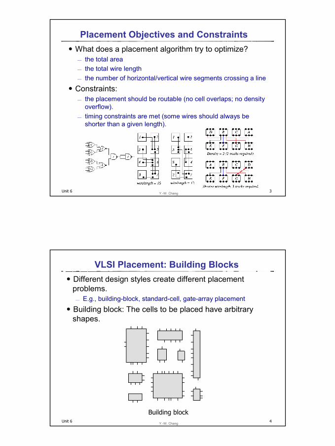
VLSI Placement: Standard Cells˙Standard cells are designed in such a way that power

and clock connections run horizontally through the cell and other I/O leaves the cell from the top or bottom sides.

˙The cells are placed in rows.˙Sometimes feedthrough cells are added to ease wiring.

feedthrough

Unit 6 6Y.-W. Chang

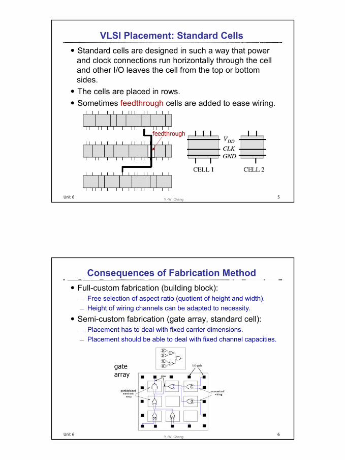
Consequences of Fabrication Method˙Full-custom fabrication (building block):

Free selection of aspect ratio (quotient of height and width). Height of wiring channels can be adapted to necessity.

˙Semi-custom fabrication (gate array, standard cell): Placement has to deal with fixed carrier dimensions. Placement should be able to deal with fixed channel capacities.

gate array

4

Unit 6 7Y.-W. Chang

Relation with Routing˙Ideally, placement and routing should be performed

simultaneously as they depend on each other’s results. This is, however, too complicated. P&R: placement and routing

˙In practice placement is done prior to routing. The placement algorithm estimates the wire length of a net using some metric.

Unit 6 8Y.-W. Chang

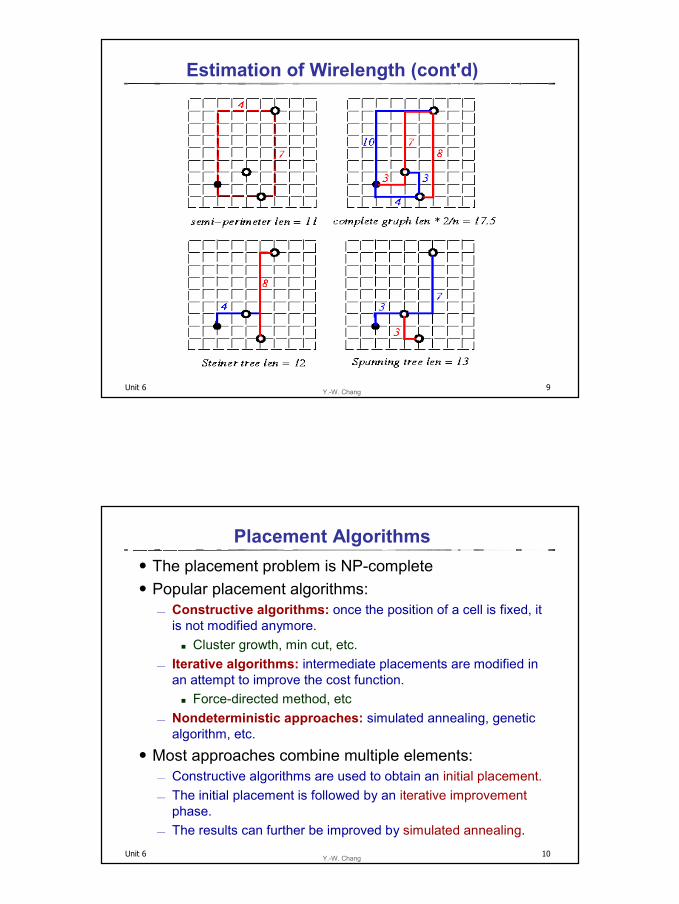
Estimation of Wirelength˙Semi-perimeter method: Half the perimeter of the bounding

rectangle that encloses all the pins of the net to be connected.Most widely used approximation!

˙Squared Euclidean distance: Squares of all pairwise terminal distances in a net using a quadratic cost function

˙Steiner-tree approximation: Computationally expensive.˙Minimum spanning tree: Good approximation to Steiner trees.˙Complete graph: Since #edges in a complete graph is =

r # of tree edges (n-1), wirelength ≈ ∑(i, j) ∈ netdist(i, j).

( 1)2

n n −

2n 2

n

5

Unit 6 9Y.-W. Chang

Estimation of Wirelength (cont'd)

Unit 6 10Y.-W. Chang

Placement Algorithms˙The placement problem is NP-complete˙Popular placement algorithms:

Constructive algorithms: once the position of a cell is fixed, it is not modified anymore.

Cluster growth, min cut, etc. Iterative algorithms: intermediate placements are modified in

an attempt to improve the cost function.Force-directed method, etc

Nondeterministic approaches: simulated annealing, genetic algorithm, etc.

˙Most approaches combine multiple elements: Constructive algorithms are used to obtain an initial placement. The initial placement is followed by an iterative improvement

phase. The results can further be improved by simulated annealing.

6

Unit 6 11Y.-W. Chang

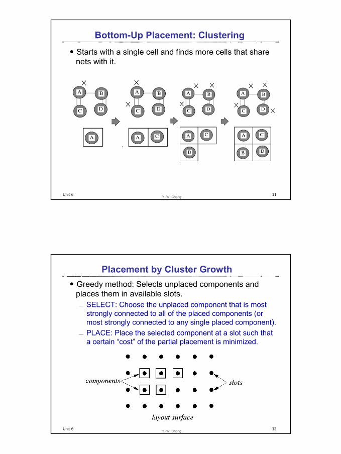
Bottom-Up Placement: Clustering˙Starts with a single cell and finds more cells that share

nets with it.

Unit 6 12Y.-W. Chang

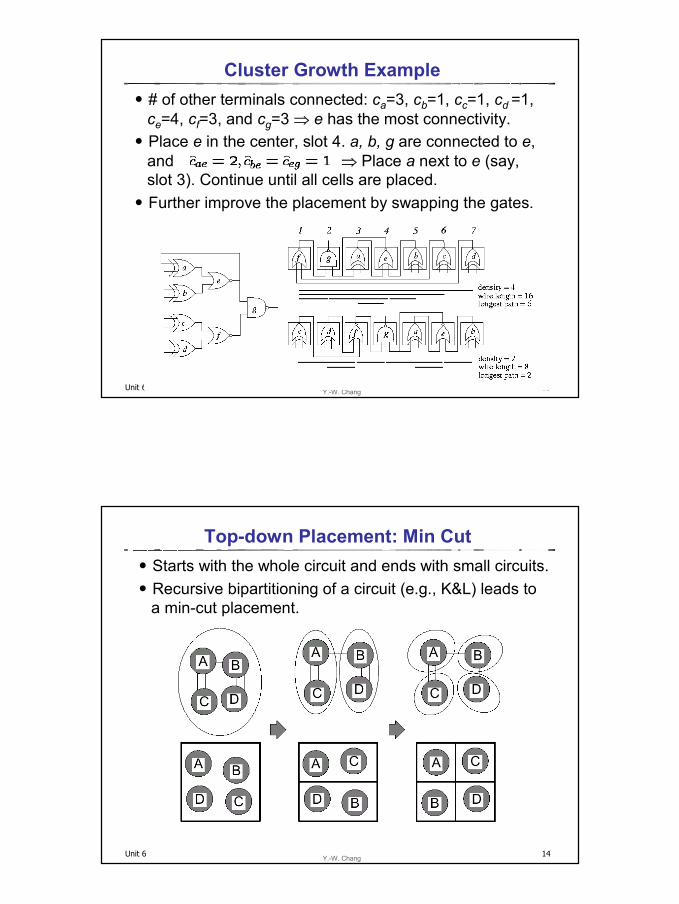
Placement by Cluster Growth˙Greedy method: Selects unplaced components and

places them in available slots. SELECT: Choose the unplaced component that is most

strongly connected to all of the placed components (or most strongly connected to any single placed component).

PLACE: Place the selected component at a slot such that a certain “cost” of the partial placement is minimized.

7

Unit 6 13Y.-W. Chang

Cluster Growth Example˙# of other terminals connected: ca=3, cb=1, cc=1, cd =1,

ce=4, cf=3, and cg=3 ⇒ e has the most connectivity.˙Place e in the center, slot 4. a, b, g are connected to e,

and ⇒ Place a next to e (say, slot 3). Continue until all cells are placed.

˙Further improve the placement by swapping the gates.

Unit 6 14Y.-W. Chang

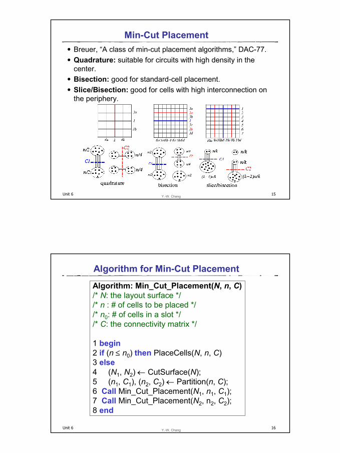
Top-down Placement: Min Cut˙Starts with the whole circuit and ends with small circuits.˙Recursive bipartitioning of a circuit (e.g., K&L) leads to

a min-cut placement.

8

Unit 6 15Y.-W. Chang

Min-Cut Placement˙Breuer, “A class of min-cut placement algorithms,” DAC-77.˙Quadrature: suitable for circuits with high density in the

center.˙Bisection: good for standard-cell placement.˙Slice/Bisection: good for cells with high interconnection on

the periphery.

Unit 6 16Y.-W. Chang

Algorithm for Min-Cut PlacementAlgorithm: Min_Cut_Placement(N, n, C)/* N: the layout surface *//* n : # of cells to be placed *//* n0: # of cells in a slot */ /* C: the connectivity matrix */

1 begin2 if (n ≤ n0) then PlaceCells(N, n, C)3 else4 (N1, N2) ← CutSurface(N);5 (n1, C1), (n2, C2) ← Partition(n, C); 6 Call Min_Cut_Placement(N1, n1, C1); 7 Call Min_Cut_Placement(N2, n2, C2); 8 end

9

Unit 6 17Y.-W. Chang

Quadrature Placement Example˙Apply the K-L heuristic to partition + Quadrature

Placement: Cost C1 = 4, C2L= C2R = 2, etc.

Unit 6 18Y.-W. Chang

Min-Cut Placement with Terminal Propagation˙Dunlop & Kernighan, “A procedure for placement of

standard-cell VLSI circuits,” IEEE TCAD, Jan. 1985.˙Drawback of the original min-cut placement: Does not

consider the positions of terminal pins that enter a region. What happens if we swap {1, 3, 6, 9} and {2, 4, 5, 7} in

the previous example?

10

Unit 6 19Y.-W. Chang

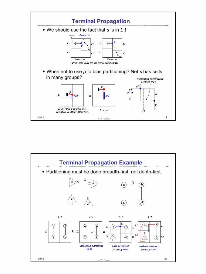
Terminal Propagation˙We should use the fact that s is in L1!

˙When not to use p to bias partitioning? Net s has cells in many groups?

Unit 6 20Y.-W. Chang

Terminal Propagation Example˙Partitioning must be done breadth-first, not depth-first.

11

Unit 6 21Y.-W. Chang

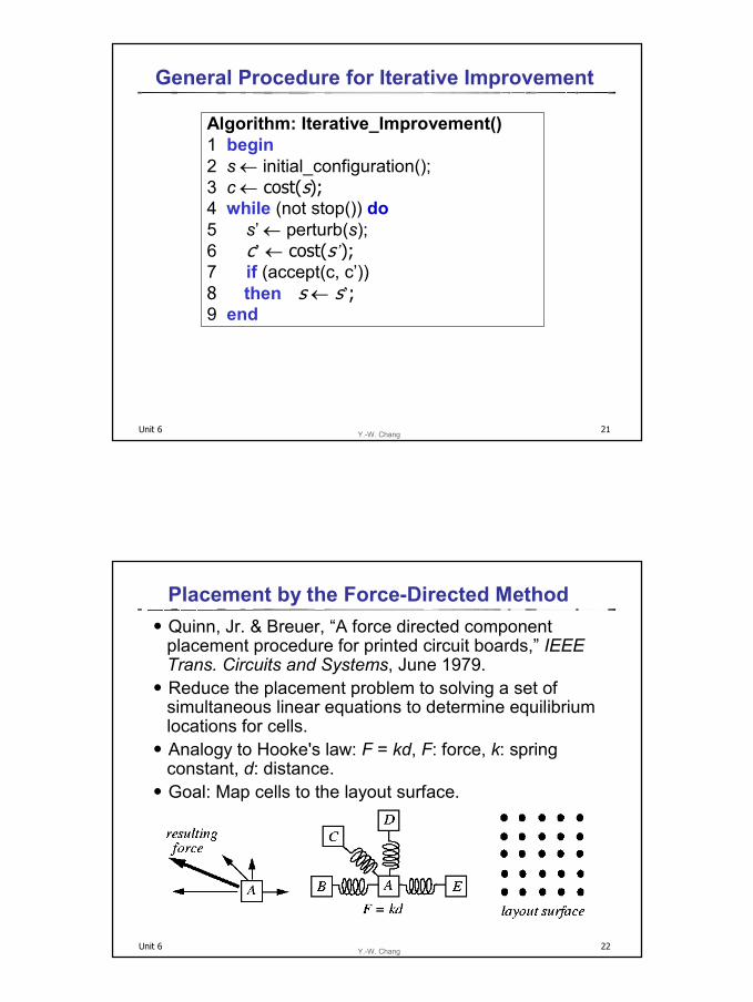
General Procedure for Iterative Improvement

Algorithm: Iterative_Improvement()1 begin2 s ← initial_configuration();3 c ← cost(s);4 while (not stop()) do5 s’ ← perturb(s); 6 c’ ← cost(s’); 7 if (accept(c, c’))8 then s ← s’;9 end

Unit 6 22Y.-W. Chang

Placement by the Force-Directed Method˙Quinn, Jr. & Breuer, “A force directed component

placement procedure for printed circuit boards,” IEEE Trans. Circuits and Systems, June 1979.

˙Reduce the placement problem to solving a set of simultaneous linear equations to determine equilibrium locations for cells.

˙Analogy to Hooke's law: F = kd, F: force, k: spring constant, d: distance.

˙Goal: Map cells to the layout surface.

12

Unit 6 23Y.-W. Chang

Finding the Zero-Force Target Location˙Cell i connects to several cells j's at distances dij's by wires of

weights wij's. Total force: Fi = ∑jwijdij

˙The zero-force target location ( , ) can be determined by equating the x- and y-components of the forces to zero:

˙ In the example, and = 1.50.

x̂̂x

Unit 6 24Y.-W. Chang

Force-Directed Placement˙Can be constructive or iterative:

Start with an initial placement. Select a “most profitable” cell p (e.g., maximum F, critical

cells) and place it in its zero-force location. “Fix” placement if the zero-location has been occupied by

another cell q.˙Popular options to fix:

Ripple move: place p in the occupied location, compute a new zero-force location for q, …

Chain move: place p in the occupied location, move q to an adjacent location, …

Move p to a free location close to q.

13

Unit 6 25Y.-W. Chang

Unit 6 26Y.-W. Chang

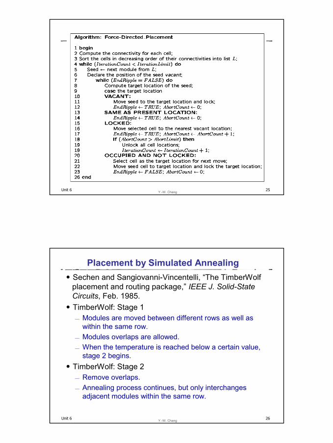
Placement by Simulated Annealing˙Sechen and Sangiovanni-Vincentelli, “The TimberWolf

placement and routing package,” IEEE J. Solid-State Circuits, Feb. 1985.

˙TimberWolf: Stage 1 Modules are moved between different rows as well as

within the same row. Modules overlaps are allowed. When the temperature is reached below a certain value,

stage 2 begins.˙TimberWolf: Stage 2

Remove overlaps. Annealing process continues, but only interchanges

adjacent modules within the same row.

14

Unit 6 27Y.-W. Chang

Solution Space & Neighborhood Structure˙Solution Space: All possible arrangements of the

modules into rows, possibly with overlaps.˙Neighborhood Structure: 3 types of moves

M1: Displace a module to a new location. M2: Interchange two modules. M3: Change the orientation of a module.

Unit 6 28Y.-W. Chang

Neighborhood Structure˙TimberWolf first tries to select a move between M1 and M2: Prob(M1)

= 0.8, Prob(M2) = 0.2.˙ If a move of type M1 is chosen and it is rejected, then a move of type

M3 for the same module will be chosen with probability 0.1.˙Restrictions: (1) what row for a module can be displaced? (2) what

pairs of modules can be interchanged?˙Key: Range Limiter

At the beginning, (WT, HT) is big enough to contain the whole chip. Window size shrinks as temperature decreases. Height & width ∝ log(T). Stage 2 begins when window size is so small that no inter-row module

interchanges are possible.

15

Unit 6 29Y.-W. Chang

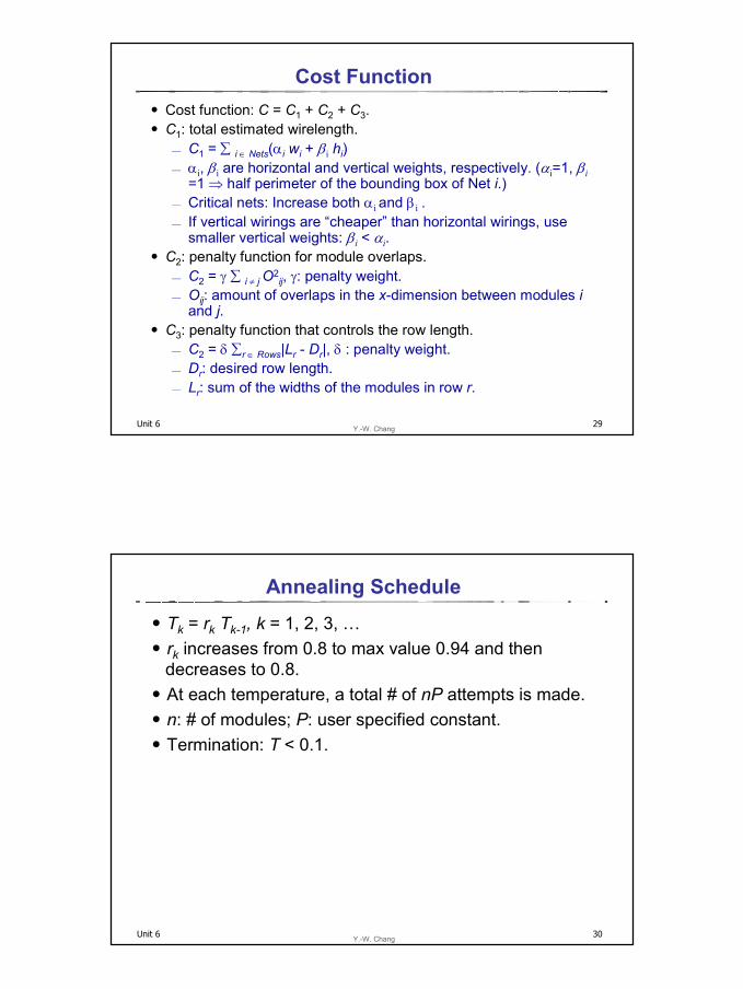
Cost Function˙Cost function: C = C1 + C2 + C3.˙C1: total estimated wirelength.

C1 = ∑ i ∈ Nets(αi wi + βi hi) αi, βi are horizontal and vertical weights, respectively. (αi=1, βi

=1 ⇒ half perimeter of the bounding box of Net i.) Critical nets: Increase both αi and βi . If vertical wirings are “cheaper” than horizontal wirings, use

smaller vertical weights: βi < αi.˙C2: penalty function for module overlaps.

C2 = γ ∑ i ≠ j O2ij, γ: penalty weight.

Oij: amount of overlaps in the x-dimension between modules iand j.

˙C3: penalty function that controls the row length. C2 = δ ∑r ∈ Rows|Lr - Dr|, δ : penalty weight. Dr: desired row length. Lr: sum of the widths of the modules in row r.

Unit 6 30Y.-W. Chang

Annealing Schedule˙Tk = rk Tk-1, k = 1, 2, 3, …˙rk increases from 0.8 to max value 0.94 and then

decreases to 0.8.˙At each temperature, a total # of nP attempts is made.˙n: # of modules; P: user specified constant.˙Termination: T < 0.1.

16

Unit 6 31Y.-W. Chang

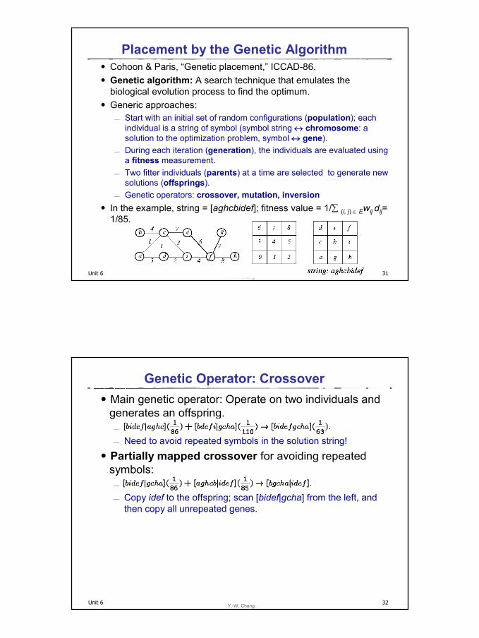
Placement by the Genetic Algorithm˙Cohoon & Paris, “Genetic placement,” ICCAD-86.˙Genetic algorithm: A search technique that emulates the

biological evolution process to find the optimum.˙Generic approaches:

Start with an initial set of random configurations (population); each individual is a string of symbol (symbol string ↔ chromosome: a solution to the optimization problem, symbol ↔ gene).

During each iteration (generation), the individuals are evaluated using a fitness measurement.

Two fitter individuals (parents) at a time are selected to generate new solutions (offsprings).

Genetic operators: crossover, mutation, inversion˙ In the example, string = [aghcbidef]; fitness value = 1/∑ (i, j) ∈ Ewij dij=

1/85.

Unit 6 32Y.-W. Chang

Genetic Operator: Crossover˙Main genetic operator: Operate on two individuals and

generates an offspring.

Need to avoid repeated symbols in the solution string!˙Partially mapped crossover for avoiding repeated

symbols:

Copy idef to the offspring; scan [bidef|gcha] from the left, and then copy all unrepeated genes.

17

Unit 6 33Y.-W. Chang

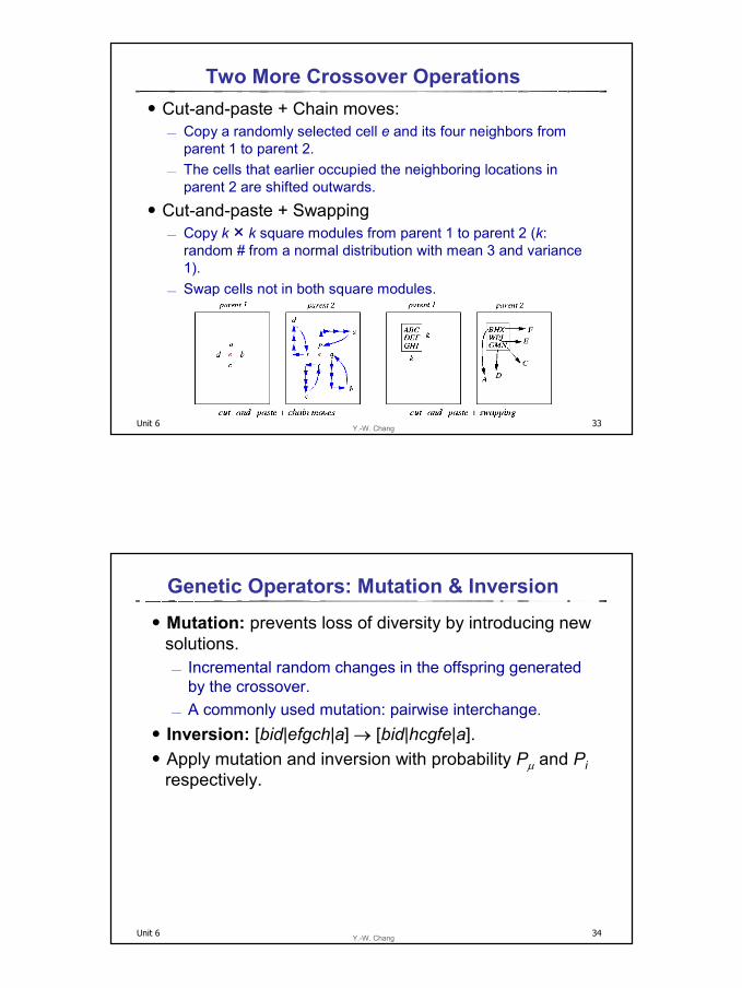
Two More Crossover Operations˙Cut-and-paste + Chain moves:

Copy a randomly selected cell e and its four neighbors from parent 1 to parent 2.

The cells that earlier occupied the neighboring locations in parent 2 are shifted outwards.

˙Cut-and-paste + Swapping Copy k r k square modules from parent 1 to parent 2 (k:

random # from a normal distribution with mean 3 and variance 1).

Swap cells not in both square modules.

Unit 6 34Y.-W. Chang

Genetic Operators: Mutation & Inversion˙Mutation: prevents loss of diversity by introducing new

solutions. Incremental random changes in the offspring generated

by the crossover. A commonly used mutation: pairwise interchange.

˙Inversion: [bid|efgch|a] → [bid|hcgfe|a].˙Apply mutation and inversion with probability Pµ and Pi

respectively.

18

Unit 6 35Y.-W. Chang

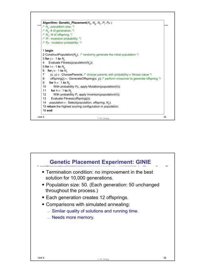
Algorithm: Genetic_Placement(Np, Ng, No, Pi, Pµ )/* Np: population size; */ /* Ng: # of generation; */ /* No: \# of offspring; */ /* Pi : inversion probability; */ /* Pµ : mutation probability; */

1 begin2 ConstructPopulation(Ng); /* randomly generate the initial population */ 3 for j ← 1 to Np4 Evaluate Fitness(population(Np)); 5 for i ← 1 to Ng6 for j ← 1 to No7 (x, y) ← ChooseParents; /* choose parents with probability ∝ fitness value */8 offspring(j) ← GenerateOffspring(x, y); /* perform crossover to generate offspring */9 for h ← 1 to Np10 With probability Pµ, apply Mutation(population(h));11 for h ← 1 to Np12 With probability Pi, apply Inversion(population(h));13 Evaluate Fitness(offspring(j));14 population ← Select(population, offspring, Np); 15 return the highest scoring configuration in population; 16 end

Unit 6 36Y.-W. Chang

Genetic Placement Experiment: GINIE˙Termination condition: no improvement in the best

solution for 10,000 generations.˙Population size: 50. (Each generation: 50 unchanged

throughout the process.)˙Each generation creates 12 offsprings.˙Comparisons with simulated annealing:

Similar quality of solutions and running time. Needs more memory.