UNIT 8 PRICING STRATEGIES AND PRACTICES …application.dbuglobal.com/assets/Pu18ME1002/CPu18ME1002...NOTES Self-Instructional Material 243 Pricing Strategies and Practices UNIT 8 PRICING

UNIT 8 PRICING STRATEGIES AND PRACTICES

MODULE - 2

M

O

D

U

L

E

-

1

NOTES

Self-Instructional Material 243

Pricing Strategies and Practices

UNIT 8 PRICING STRATEGIES ANDPRACTICES

Structure

8.0 Introduction8.1 Unit Objectives8.2 Cost-plus Pricing

8.2.1 Cost-plus Pricing and Marginal Rule Pricing8.3 Multiple Product Pricing8.4 Pricing In Life-cycle of a Product

8.4.1 Pricing a New Product; 8.4.2 Pricing in Maturity Period8.4.3 Pricing a Product in Decline

8.5 Pricing in Relation to Established Products8.5.1 Pricing Below the Market Price; 8.5.2 Pricing at Market Price8.5.3 Pricing Above the Existing Market Price

8.6 Transfer Pricing8.6.1 Transfer Pricing without External Market;8.6.2 Transfer Pricing with External Competitive Market;8.6.3 Transfer Pricing Under Imperfect External Market

8.7 Competitive Bidding of Price8.7.1 Major Factors in Competitive Bidding; 8.7.2 Determining the Competitive Bid

8.8 Peak Load Pricing8.9.1 Problems in Pricing; 8.9.2 Double Pricing System

8.9 Summary8.10 Answers to ‘Check Your Progress’8.11 Exercises and Questions8.12 Further Reading

8.0 INTRODUCTION

Pricing theory under the profit maximization hypothesis suggests that, given the revenueand cost curves, price and output are so determined that profit is maximised. Someempiricists have, however, produced the evidence, inadequate though, that firms followa pricing rule other than the one suggested by the marginality, rule. Besides, in a complexbusiness world, business firms follow a variety of pricing rules and methods dependingon the conditions faced by them. In this chapter, we will discuss some important pricingstrategies and pricing practices.

8.1 UNIT OBJECTIVES

To show that pricing practices often differ from pricing theoryTo discuss various pricing practices of business firmsTo show how firms price their product used by themselves

NOTES

244 Self-Instructional Material

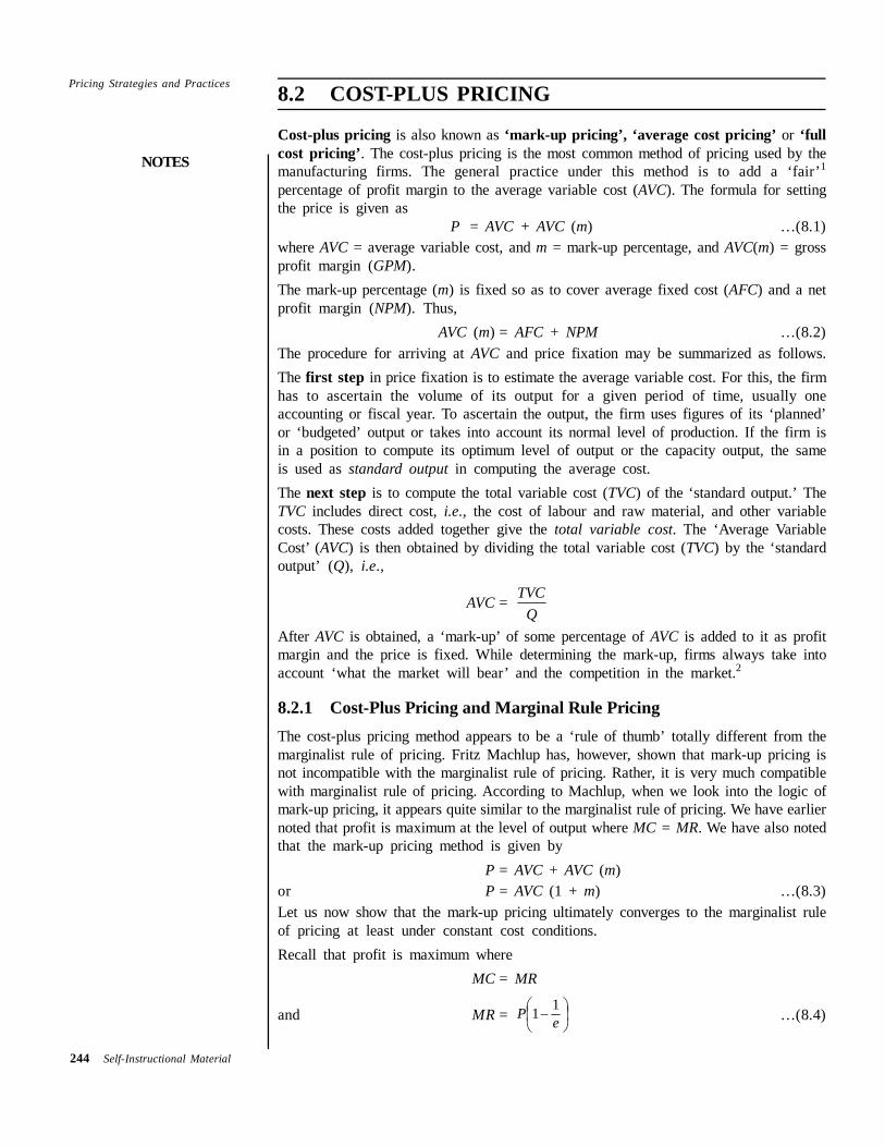
Pricing Strategies and Practices 8.2 COST-PLUS PRICING

Cost-plus pricing is also known as ‘mark-up pricing’, ‘average cost pricing’ or ‘fullcost pricing’. The cost-plus pricing is the most common method of pricing used by themanufacturing firms. The general practice under this method is to add a ‘fair’1

percentage of profit margin to the average variable cost (AVC). The formula for settingthe price is given as

P = AVC + AVC (m) …(8.1)where AVC = average variable cost, and m = mark-up percentage, and AVC(m) = grossprofit margin (GPM).The mark-up percentage (m) is fixed so as to cover average fixed cost (AFC) and a netprofit margin (NPM). Thus,

AVC (m) = AFC + NPM …(8.2)The procedure for arriving at AVC and price fixation may be summarized as follows.The first step in price fixation is to estimate the average variable cost. For this, the firmhas to ascertain the volume of its output for a given period of time, usually oneaccounting or fiscal year. To ascertain the output, the firm uses figures of its ‘planned’or ‘budgeted’ output or takes into account its normal level of production. If the firm isin a position to compute its optimum level of output or the capacity output, the sameis used as standard output in computing the average cost.The next step is to compute the total variable cost (TVC) of the ‘standard output.’ TheTVC includes direct cost, i.e., the cost of labour and raw material, and other variablecosts. These costs added together give the total variable cost. The ‘Average VariableCost’ (AVC) is then obtained by dividing the total variable cost (TVC) by the ‘standardoutput’ (Q), i.e.,

AVC = TVCQ

After AVC is obtained, a ‘mark-up’ of some percentage of AVC is added to it as profitmargin and the price is fixed. While determining the mark-up, firms always take intoaccount ‘what the market will bear’ and the competition in the market.2

8.2.1 Cost-Plus Pricing and Marginal Rule PricingThe cost-plus pricing method appears to be a ‘rule of thumb’ totally different from themarginalist rule of pricing. Fritz Machlup has, however, shown that mark-up pricing isnot incompatible with the marginalist rule of pricing. Rather, it is very much compatiblewith marginalist rule of pricing. According to Machlup, when we look into the logic ofmark-up pricing, it appears quite similar to the marginalist rule of pricing. We have earliernoted that profit is maximum at the level of output where MC = MR. We have also notedthat the mark-up pricing method is given by

P = AVC + AVC (m)or P = AVC (1 + m) …(8.3)Let us now show that the mark-up pricing ultimately converges to the marginalist ruleof pricing at least under constant cost conditions.Recall that profit is maximum where

MC = MR

and MR = ⎟⎠⎞

⎜⎝⎛ − eP 11 …(8.4)

NOTES


Pricing Strategies and Practices

or MR = 1ePe−⎛ ⎞

⎜ ⎟⎝ ⎠…(8.5)

By substituting Eq. (8.5) in Eq. (8.4), we may restate the necessary condition of profitmaximization as

MC = 1ePe−⎛ ⎞

⎜ ⎟⎝ ⎠…(8.6)

If MC is constant, then MC = AVC. By substituting AVC for MC, Eq. (8.6) maybe rewritten as,

AVC = 1ePe−⎛ ⎞

⎜ ⎟⎝ ⎠…(8.7)

By rearranging the terms in Eq. (8.7), we get

P = 1eAVCe−⎛ ⎞+⎜ ⎟⎝ ⎠

or P = 1

eAVCe

⎛ ⎞⎜ ⎟⎝ ⎠−

...(8.8)

Now, consider Eq. (8.6). If MC > 0, then 1ePe−⎛ ⎞

⎜ ⎟⎝ ⎠ must be greater than 0. For

1ePe−⎛ ⎞

⎜ ⎟⎝ ⎠ to be greater than 0, e must be greater than 1. This implies that profit canbe maximised only when e > 1. The logic to this conclusion can be provided as follows.

Given the Eq. 8.5 and Eq. 8.6, if e = 1, MR = 0, and if e < 1, MR < 0. It meansthat if MR < 0 and MC > 0, or in other words, when MR π MC, then the rule of profitmaximization breaks down. Thus, profit can be maximized only if e > 1, and MC > 0.Now if e > 1, then the term e/(e – 1) will always be greater than 1 by an amount, saym. Then

1e

e −= (1 + m) ...(8.9)

By substituting term (1 + m) in Eq. (8.9) for e/(e – 1) in Eq. (8.7), we getP = AVC (1 + m) …(8.10)

where m denotes the mark-up rate.Note that Eq. (8.10) is exactly the same as Eq. (8.3). This means that the mark-up ruleof pricing converges into the marginalist rule of pricing. In other words, it is proved thatthe mark-up pricing method leads to the marginalist rule of pricing. However, m in Eq.(8.3) and in (8.9) need not the same.Limitations of Mark-up Pricing Rule. The cost-plus pricing has certain limitations, whichshould be borne in mind while using this method for price fixation.First, cost-plus pricing assumes that a firm’s resources are optimally allocated and thestandard cost of production is comparable with the average of the industry. In reality,however, it may not be so and cost estimates based on these assumptions may be anoverestimate or an underestimate. Under these conditions pricing may not be commen-surate with the objective of the firm.Second, in cost-plus pricing, generally, historical cost rather than current cost data areused. This may lead to under-pricing under increasing cost conditions and to over-pricing under decreasing cost conditions, which may go against the firm’s objective.Third, if variable cost fluctuates frequently and significantly, cost-plus pricing may notbe an appropriate method of pricing.

NOTES


Pricing Strategies and Practices Finally, it is also alleged that cost-plus pricing ignores the demand side of the market andis solely based on supply conditions. This is, however, not true, because the firmdetermines the mark-up on the basis of ‘what the market can bear’ and it does take intoaccount the elasticity aspect of the demand for the product, as shown above.

8.3 MULTIPLE PRODUCT PRICING

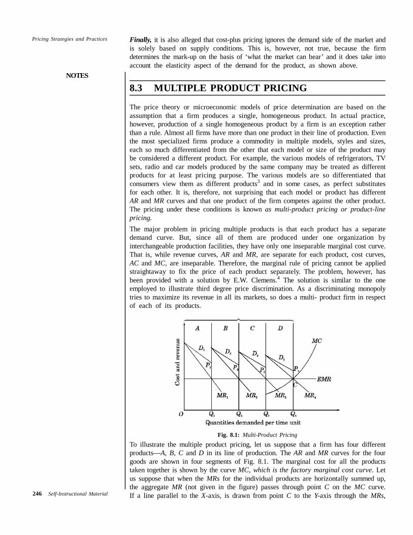
The price theory or microeconomic models of price determination are based on theassumption that a firm produces a single, homogeneous product. In actual practice,however, production of a single homogeneous product by a firm is an exception ratherthan a rule. Almost all firms have more than one product in their line of production. Eventhe most specialized firms produce a commodity in multiple models, styles and sizes,each so much differentiated from the other that each model or size of the product maybe considered a different product. For example, the various models of refrigerators, TVsets, radio and car models produced by the same company may be treated as differentproducts for at least pricing purpose. The various models are so differentiated thatconsumers view them as different products3 and in some cases, as perfect substitutesfor each other. It is, therefore, not surprising that each model or product has differentAR and MR curves and that one product of the firm competes against the other product.The pricing under these conditions is known as multi-product pricing or product-linepricing.The major problem in pricing multiple products is that each product has a separatedemand curve. But, since all of them are produced under one organization byinterchangeable production facilities, they have only one inseparable marginal cost curve.That is, while revenue curves, AR and MR, are separate for each product, cost curves,AC and MC, are inseparable. Therefore, the marginal rule of pricing cannot be appliedstraightaway to fix the price of each product separately. The problem, however, hasbeen provided with a solution by E.W. Clemens.4 The solution is similar to the oneemployed to illustrate third degree price discrimination. As a discriminating monopolytries to maximize its revenue in all its markets, so does a multi- product firm in respectof each of its products.

Fig. 8.1: Multi-Product PricingTo illustrate the multiple product pricing, let us suppose that a firm has four differentproducts—A, B, C and D in its line of production. The AR and MR curves for the fourgoods are shown in four segments of Fig. 8.1. The marginal cost for all the productstaken together is shown by the curve MC, which is the factory marginal cost curve. Letus suppose that when the MRs for the individual products are horizontally summed up,the aggregate MR (not given in the figure) passes through point C on the MC curve.If a line parallel to the X-axis, is drawn from point C to the Y-axis through the MRs,

NOTES


Pricing Strategies and Practicesthe intersecting points will show the points where MC and MRs are equal for eachproduct, as shown by the line EMR, the Equal Marginal Revenue line. The points ofintersection between EMR and MRs determine the output level and price for eachproduct. The output of the four products are given as OQ1 of product A; Q1Q2 of B;Q2Q3 of C; and Q3Q4 of D. The respective prices for the four products are: P1Q1 forproduct A; P2Q2 for B; P3Q3 for C, and P4Q4 for D. These price and output combi-nations maximize the profit from each product and hence the overall profit of the firm.

8.4 PRICING IN LIFE-CYCLE OF A PRODUCT

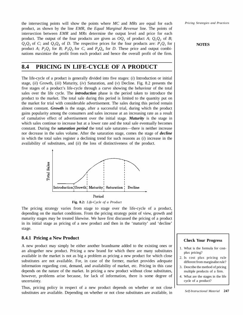
The life-cycle of a product is generally divided into five stages: (i) Introduction or initialstage, (ii) Growth, (iii) Maturity, (iv) Saturation, and (v) Decline. Fig. 8.2 presents thefive stages of a product’s life-cycle through a curve showing the behaviour of the totalsales over the life cycle. The introduction phase is the period taken to introduce theproduct to the market. The total sale during this period is limited to the quantity put onthe market for trial with considerable advertisement. The sales during this period remainalmost constant. Growth is the stage, after a successful trial, during which the productgains popularity among the consumers and sales increase at an increasing rate as a resultof cumulative effect of advertisement over the initial stage. Maturity is the stage inwhich sales continue to increase but at a lower rate and the total sale eventually becomesconstant. During the saturation period the total sale saturates—there is neither increasenor decrease in the sales volume. After the saturation stage, comes the stage of declinein which the total sales register a declining trend for such reasons as (i) increase in theavailability of substitutes, and (ii) the loss of distinctiveness of the product.

Fig. 8.2: Life-Cycle of a Product

The pricing strategy varies from stage to stage over the life-cycle of a product,depending on the market conditions. From the pricing strategy point of view, growth andmaturity stages may be treated likewise. We have first discussed the pricing of a productin its initial stage as pricing of a new product and then in the ‘maturity’ and ‘decline’stage.

8.4.1 Pricing a New ProductA new product may simply be either another brandname added to the existing ones oran altogether new product. Pricing a new brand for which there are many substitutesavailable in the market is not as big a problem as pricing a new product for which closesubstitutes are not available. For, in case of the former, market provides adequateinformation regarding cost, demand, and availability of market, etc. Pricing in this casedepends on the nature of the market. In pricing a new product without close substitutes,however, problems arise because, for lack of information, there is some degree ofuncertainty.Thus, pricing policy in respect of a new product depends on whether or not closesubstitutes are available. Depending on whether or not close substitutes are available, in

Check Your Progress

1. What is the formula for cost-plus pricing?

2. Is cost plus pricing ruledifferent from marginalist rule?

3. Describe the method of pricingmultiple products of a firm.

4. What are the stages in the lifecycle of a product?

NOTES


Pricing Strategies and Practices pricing a new product, generally two kinds of pricing strategies are suggested, viz., (i)skimming price policy; and (ii) penetration price policy.

(i) Skimming price policy. The skimming price policy is adopted where closesubstitutes of a new product are not available. This pricing strategy is intendedto skim the cream of the market, i.e., consumer’s surplus, by setting a highinitial price, three or four times the ex-factory price, and a subsequent loweringof prices in a series of reduction, especially in case of consumer durables. Theinitial high price would generally be accompanied by heavy sales promotingexpenditure. This policy succeeds for the following reasons.First, in the initial stage of the introduction of product, demand is relativelyinelastic because of consumers’ desire for distinctiveness by the consumptionof a new product.Second, cross-elasticity is usually very low for lack of a close substitute.Third, step-by-step price-cuts help skimming consumers’ surplus available at thelower segments of demand curve.Fourth, high initial prices are helpful in recouping the development costs.The post-skimming strategy includes the decisions regarding the time and sizeof price reduction. The appropriate occasion for price reduction is the time ofsaturation of the top-level demand or when a strong competition isapprehended. As regards the rate of price reduction, when the product is on itsway to losing its distinctiveness, the price-cut should be appropriately larger.But, if the product has retained its exclusiveness, a series of small pricereductions would be more appropriate.

(ii) Penetration price policy. In contrast to skimming price policy, the penetrationprice policy involves a reverse strategy. This pricing policy is adopted generallyin the case of new products for which substitutes are available. This policyrequires fixing a lower initial price designed to penetrate the market as quicklyas possible and is intended to maximize the profits in the long-run. Therefore,the firms pursuing the penetration price policy set a low price of the productin the initial stage. As the product catches the market, price is gradually raisedup. The success of penetration price policy requires the existence of thefollowing conditions.First, the short run demand for the product should have an elasticity greaterthan unity. It helps in capturing the market at lower prices.Second, economies of large-scale production are available to the firm with theincrease in sales. Otherwise, increase in production would result in increase incosts which might reduce the competitiveness of the price.Third, the potential market for the product is fairly large and has a good dealof future prospects.Fourth, the product should have a high cross-elasticity in relation to rivalproducts for the initial lower price to be effective.Finally, the product, by nature should be such that it can be easily accepted andadopted by the consumers.

The choice between the two strategic price policies depends on (i) the rate of marketgrowth; (ii) the rate of erosion of distinctiveness; and (iii) the cost-structure of theproducers. If the rate of market growth is slow for such reasons as lack of information,consumers’ hesitation, etc., penetration price policy would be unsuitable. The reason is alow price will not mean a large sale. If the pioneer product is likely to lose itsdistinctiveness at a faster rate skimming price policy would be unsuitable: it should befollowed when lead time, i.e., the period of distinctiveness is fairly long. If cost-structure

NOTES


Pricing Strategies and Practicesshows increasing returns over time, penetration price policy would be more suitable, sinceit enables the producer to reduce his cost and prevents potential competitors from enteringthe market in the short-run.

8.4.2 Pricing in Maturity PeriodMaturing period is the second stage in the life-cycle of a product. It is a stage betweenthe growth period and decline period of sales. Sometimes maturity period is bracketedwith saturation period. Maturity period may also be defined as the period of decline inthe growth rate of sales (not the total sales) and the period of zero growth rate. Theconcept of maturity period is useful to the extent it gives out signals for takingprecaution in regard to pricing policy. However, the concept itself does not provideguidelines for the pricing policy. Joel Dean5 suggests that the “first step for the manu-facturer whose speciality is about to slip into the commodity category is to reduce real… prices as soon as the system of deterioration appears.” But he warns that “this doesnot mean that the manufacturer should declare open price war in the industry”. Heshould rather move in the direction of “product improvement and market segmentation”.

8.4.3 Pricing a Product in DeclineThe product in decline is one that enters the post-maturity stage. In this stage, the totalsale of the product starts declining. The first step in pricing strategy in this stage isobviously to reduce the price. The product should be reformulated and remodelled to suitthe consumers’ preferences. It is a common practice in the book trade. When the saleof a hard-bound edition reaches saturation, paper-back edition is brought into the market.This facility is, however, limited to only a few commodities. As a final step in thestrategy, the advertisement expenditure may be reduced drastically or withdrawncompletely, and rely on the residual market. This, however, requires a strong will of theproducer.

8.5 PRICING IN RELATION TO ESTABLISHEDPRODUCTS

Many producers enter the market often with a new brand of a commodity for whicha number of substitutes are available. For example, the cold drinks like Coke and Spot,were quite popular in the market when new brands of cold drinks like Limca, ThumsUp, Double Seven, Mirinda, Pepsi, Teem, Campa, etc., were introduced in the marketover time. So has been the case with many consumer goods. Many other models ofmotor cars appeared in the market despite the popularity of Maruti cars. A new entrantto the market faces the problem of pricing his product because of strong competitionwith established products. This problem of pricing of a new brand is known as pricingin relation to the established products.In pricing a product in relation to its well established substitutes, generally three typesof pricing strategies are adopted, viz., (i) pricing below the ongoing price, (ii) pricingat par with the prevailing market price, and (iii) pricing above the existing market price.Let us now see which of these strategies are adopted under what conditions.

8.5.1 Pricing Below the Market PricePricing below the prevailing market price of the substitutes is generally preferred undertwo conditions. First, if a firm wants to expand its product-mix with a view to utilizingits unused capacity in the face of tough competition with the established brands, thestrategy of pricing below the market price is generally adopted. This strategy gives the new

NOTES


Pricing Strategies and Practices brand an opportunity to gain popularity and establish itself. For this, however, a high cross-elasticity of demand between the substitute brands is necessary. This strategy may,however, not work if existing brands have earned a strong brand loyalty of the consumers.If so, the price incentive from the new producers must, therefore, overweigh the brandloyalty of the consumers of the established products, and must also be high enough toattract new consumers. This strategy is similar to the penetrating pricing. Second, thistechnique has been found to be more successful in the case of innovative products. Whenthe innovative product gains popularity, the price may be gradually raised to the level ofmarket price.

8.5.2 Pricing at Market PricePricing at par with the market price of the existing brands is considered to be the mostreasonable pricing strategy for a product which is being sold in a strongly competitivemarket. In such a market, keeping the price below the market price is not of much availbecause the product can be sold in any quantity at the existing market rate. This strategyis also adopted when the seller is not a ‘price leader’. It is rather a ‘price-taker’ in anoligopolistic market. This is, in fact, a very common pricing strategy—rather the mostcommon practice.

8.5.3 Pricing Above the Existing Market PriceThis strategy is adopted when a seller intends to achieve a prestigious position amongthe sellers in the market. This is a more common practice in case of products consideredto be a commodity of conspicuous consumption or prestige goods or deemed to be ofmuch superior quality. Consumers of such goods prefer shopping in a gorgeous shopof a posh locality of the city. This is known as the ‘Veblen Effect’. Sellers of such goodsrely on their customers’ high propensity to consume a prestigious commodity. After theseller achieves the distinction of selling high quality goods, though at a high price, theymay sell even the ordinary goods at a price much higher than the market price. Thispractice is common among sellers of readymade garments.

Besides, a firm may sets a high price for its product if it pursues the ‘skimming pricestrategy’. This pricing strategy is more suitable for innovative products when the firmcan be sure of the distinctiveness of its product. The demand for the commodity musthave a low cross-elasticity in respect of competing goods.

8.6 TRANSFER PRICING

The large size firms divide their operation very often into product divisions or subsidiaries.Growing firms add new divisions or departments to the existing ones. The firms thentransfer some of their activities to other divisions. The goods and services produced bythe new division are used by the parent organisation. In other words, the parent divisionbuys the product of its subsidiaries. Such firms face the problem of determining anappropriate price for the product transferred from one division or subsidiary to the other.Specifically, the problem is of determining the price of a product produced by onedivision of the same firm. This problem becomes much more difficult when each divisionhas a separate profit function to maximize. Pricing of intra-firm ‘transfer product’ isreferred to as ‘transfer pricing’. One of the most systematic treatments of the transferpricing technique has been provided by Hirshleifer.6 We will discuss here briefly histechnique of transfer pricing.To begin with, let us suppose that a refrigeration company established a decade ago usedto produce and sell refrigerators fitted with compressors bought from a compressormanufacturing company. Now the refrigeration company decides to set up its ownsubsidiary to manufacture compressors. Let us also assume:

NOTES


Pricing Strategies and Practices(i) both parent and subsidiary companies have their own profit functions tomaximize ;

(ii) the refrigeration company sells its product in a competitive market and itsdemand is given by a straight horizontal line; and

(iii) the refrigeration company uses all the compressors produced by its subsidiary.In addition, we assume that there is no external market for the compressors. We will

later drop this assumption and alternatively assume that there is an external market for thecompressors and discuss the technique of transfer pricing under both the alternativeconditions. Let us first discuss transfer pricing with no external market.

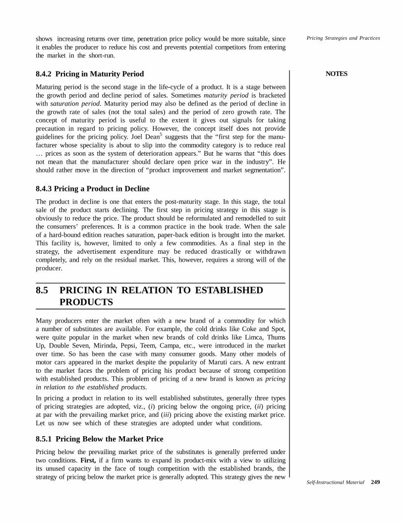
8.6.1 Transfer Pricing without External MarketGiven the foregoing assumptions, the refrigeration company has to set an appropriateprice for the compressors so that the profit of its subsidiary too is maximum. To dealwith the ‘transfer pricing’ problem, let us first look into the pricing and output deter-mination of the final product, i.e., refrigerators. Since the refrigeration company sells itsrefrige- rators presumably in a competitive market, the demand for its product is givenby a straight horizontal line as shown by the line ARr = MRr in Fig. 8.3.

Fig. 8.3: Price Determination of the Final Product (Refrigerators)

The marginal cost of intermediate good, i.e., compressor, is shown by MCc curve andthat of the refrigerator body by MCb. The MCc and MCb added vertically give thecombined marginal cost curve, the MCt. At output OQ, for example, TQ + MQ = PQ.The MCt intersects line ARr = MRr at point P. An ordinate drawn from point P downto the horizontal axis determines the most profitable outputs of refrigerator body andcompressors each at OQ. Thus, the output of both refrigerator body and compressorsis simultaneously determined. Since at OQ level of output, the firm’s MCt = MRr, therefrigerator company maximizes its profits from the final product, the refrigerators.Now, let us find the price of the compressors. The question that arises is: what shouldbe the price of the compressors so that the compressor manufacturing division toomaximizes its profit? The answer to this question can be obtained by applying themarginality principle which requires equalizing MC and MR in respect of compressors.The marginal cost curve for the compressors is given by MCc in Fig. 8.3. The firmtherefore has to obtain the marginal revenue for its compressors. The marginal revenueof the compressors (MRc) can be obtained by subtracting the non-compressor marginalcost of the final good from the MRr

7. Thus,MRc = MRr – (MCt – MCc) … (8.11)

For example, in Fig. 8.3, at output OQ, MRr = PQ, MCt = PQ, and MCc = MQ. Bysubstituting these values in Eq. 8.11, we get

NOTES


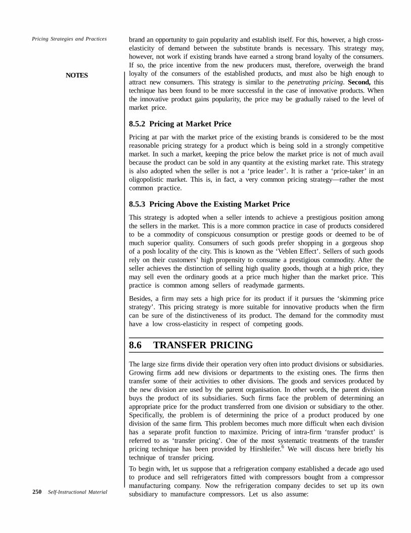
Pricing Strategies and Practices MRc = PQ – (PQ – MQ)PQ – PM = MQ

or, since in Fig.8.3, PQ – MQ = PM, and PM = TQ, therefore,MRc = PQ – TQ = PT

and PT = MQ

Fig. 8.4: Determination of Transfer Price

We may recall that ARr = MRr, i.e., MRr is constant, and that MCt is a rising function.Thus, MRr – MCc will be a decreasing function. Notice the vertical distance betweenARr = MRr line, and MCc curve is decreasing as shown in Fig. 8.3. When MRc (whichequals MRr – MCc) is obtained for different levels of output and graphed, it yields acurve like MRc curve shown in Fig. 8.4. The MCc curve (which is the same as MCccurve in Fig 8.3) intersects the MRc at point P. At point P, MRc = MCc and output isOQ. Thus, the price of compressors is determined at PQ in Fig. 8.4. This price enablesthe compressor division to maximize its own profit.

8.6.2 Transfer Pricing with External Competitive MarketWe have discussed above the transfer pricing under the assumption that there is noexternal market for the compressors. It implies that the refrigeration company was thesole purchaser of its own compressors and that the compressor division had no externalmarket for its product. Let us now discuss the transfer pricing technique assuming thatthere is an external market for the compressors. The existence of the external marketimplies that the compressor division has the opportunity to sell its surplus production toother buyers and the refrigeration company can buy compressors from other sellers ifthe compressor division fails to meet its total demand. Also assume that the externalmarket is perfectly competitive. Determination of transfer price under these conditionsis a little more complicated task.The method of transfer pricing with external market is illustrated in Fig. 8.5. Since thecompressor market is perfectly competitive, the demand for compressor is given by astraight horizontal line as shown by P2D in which case AR = MR. The marginal costcurve of the compressors is shown by MCc. The MRc curve shows the marginal netrevenue from the compressor, (See Fig. 8.5). Note that in the absence of the externalmarket, the transfer price of compressor would have been fixed at OP 1 = P ¢Q2 i.e.,the price where MRc = MCc. At this price the parent company would have boughtcompressors only from its subsidiary. But, since compressors are to be produced andsold under competitive conditions, the effective marginal cost of the compressor to therefrigeration company is the market price of the compressor, i.e., OP2. Besides, theprice OP2 is also the potential MR for the compressor division. Therefore, in order to

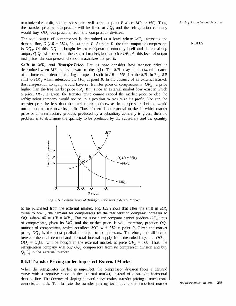
NOTES


Pricing Strategies and Practicesmaximize the profit, compressor’s price will be set at point P where MRc > MCc. Thus,the transfer price of compressor will be fixed at PQ1 and the refrigeration companywould buy OQ1 compressors from the compressor division.The total output of compressors is determined at a level where MCc intersects thedemand line, D (AR = MR), i.e., at point R. At point R, the total output of compressorsis OQ3. Of this, OQ1 is bought by the refrigeration company itself and the remainingoutput, Q1Q3 will be sold in the external market, both at price OP2. At this level of outputand price, the compressor division maximizes its profit.Shift in MRc and Transfer Price. Let us now consider how transfer price isdetermined when MRc shifts upward to the right. The MRc may shift upward becauseof an increase in demand causing an upward shift in AR = MR. Let the MRc in Fig. 8.5shift to MRć which intersects the MCc at point B. In the absence of an external market,the refrigeration company would have set transfer price of compressors at OP3—a pricehigher than the free market price OP2. But, since an external market does exist in whicha price, OP2, is given, the transfer price cannot exceed the market price or else therefrigeration company would not be in a position to maximize its profit. Nor can thetransfer price be less than the market price, otherwise the compressor division wouldnot be able to maximize its profit. Thus, if there is an external market in which marketprice of an intermediary product, produced by a subsidiary company is given, then theproblem is to determine the quantity to be produced by the subsidiary and the quantity

Fig. 8.5 Determination of Transfer Price with External Market

to be purchased from the external market. Fig. 8.5 shows that after the shift in MRccurve to MRć, the demand for compressors by the refrigeration company increases toOQ4 where AR = MR = MRć. But the subsidiary company cannot produce OQ4 unitsof compressors, given its MCc and the market price. It will, therefore, produce OQ3number of compressors, which equalizes MCc with MR at point R. Given the marketprice, OQ3 is the most profitable output of compressors. Therefore, the differencebetween the total demand and the total internal supply from the subsidiary, i.e., OQ4 –OQ3 = Q3Q4, will be bought in the external market, at price OP2 = TQ4. Thus, therefrigeration company will buy OQ3 compressors from its compressor division and buyQ3Q4 in the external market.

8.6.3 Transfer Pricing under Imperfect External MarketWhen the refrigerator market is imperfect, the compressor division faces a demandcurve with a negative slope in the external market, instead of a straight horizontaldemand line. The downward sloping demand curve makes transfer pricing a much morecomplicated task. To illustrate the transfer pricing technique under imperfect market

NOTES


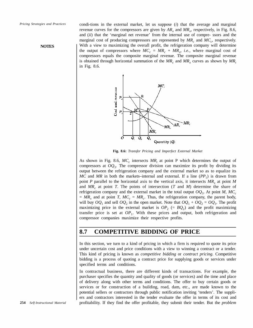
Pricing Strategies and Practices condi-tions in the external market, let us suppose (i) that the average and marginalrevenue curves for the compressors are given by ARx and MRx, respectively, in Fig. 8.6,and (ii) that the ‘marginal net revenue’ from the internal use of compressors and themarginal cost of producing compressors are represented by MRc and MCc, respectively.With a view to maximizing the overall profit, the refrigeration company will determinethe output of compressors where MCc = MRc + MRx, i.e., where marginal cost ofcompressors equals the composite marginal revenue. The composite marginal revenueis obtained through horizontal summation of the MRc and MRx curves as shown by MRtin Fig. 8.6.

Fig. 8.6: Transfer Pricing and Imperfect External Market

As shown in Fig. 8.6, MCc intersects MRt at point P which determines the output ofcompressors at OQ3. The compressor division can maximize its profit by dividing itsoutput between the refrigeration company and the external market so as to equalize itsMC and MR in both the markets–internal and external. If a line (PP1) is drawn frompoint P parallel to the horizontal axis to the vertical axis, it intersects MRx at point Mand MRc at point T. The points of intersection (T and M) determine the share ofrefrigeration company and the external market in the total output OQ3. At point M, MCc= MRx and at point T, MCc = MRc. Thus, the refrigeration company, the parent body,will buy OQ1 and sell OQ2 in the open market. Note that OQ1 + OQ2 = OQ3. The profitmaximizing price in the external market is OP2 (= BQ2) and the profit maximizingtransfer price is set at OP1. With these prices and output, both refrigeration andcompressor companies maximize their respective profits.

8.7 COMPETITIVE BIDDING OF PRICE

In this section, we turn to a kind of pricing in which a firm is required to quote its priceunder uncertain cost and price conditions with a view to winning a contract or a tender.This kind of pricing is known as competitive bidding or contract pricing. Competitivebidding is a process of quoting a contract price for supplying goods or services underspecified terms and conditions.In contractual business, there are different kinds of transactions. For example, thepurchaser specifies the quantity and quality of goods (or services) and the time and placeof delivery along with other terms and conditions. The offer to buy certain goods orservices or for construction of a building, road, dam, etc., are made known to thepotential sellers or contractors through public notification inviting ‘tenders’. The suppli-ers and contractors interested in the tender evaluate the offer in terms of its cost andprofitability. If they find the offer profitable, they submit their tender. But the problem

NOTES


Pricing Strategies and Practiceshere is not simply to quote a suitable supply price while submitting the tender. In fact,the foremost problem is to quote a supply price which can win the contract withoutunduly reducing the profit margin. For this the quoted supply price should be lower thanthat of the rival contractors.To bid a contract winning supply price is an extremely difficult task mainly because theprices of the rival firms or contractors are unknown. The problem becomes much morecomplicated if there is uncertainty about the future prices of the inputs, particularlywhen input prices are subject to fluctuation. Uncertainty about future cost conditionsincreases the degree of risk because bidding takes place at current prices and thecontracted goods and services are to be produced and supplied at future input priceswhich may be uncertain. Despite these difficulties in bidding competitive pricescontractors do quote a supply price which wins them a contract and yields profits. Letus briefly discuss the process of competitive price bidding. We assume that there areno ‘bribes’ and ‘kickbacks’.

8.7.1 Major Factors in Competitive BiddingThere are three major factors which contractors analyse in the process of competitivebidding. These are:

(i) bidder’s current and projected capacity to handle the contract,(ii) the overall objective of the bidder, and(iii) the expected bid of the rival contractors.

Bidder’s present and projected capacity to handle the contract matters a great deal incompetitive bidding. Given his present capacity, the contractor may find himself with(a) excess capacity, (b) full utilization of capacity, and (c) undertaking activity in excessof capacity. The three kinds of different capacity positions put the bidder in threedifferent positions to bid the supply price. If the bidder has an excess capacity, he maybid a price at par with his cost or even below the cost if his circumstances so demand.This kind of bidding may be motivated by the contractor’s desire (i) to popularize hisbusiness, (ii) to retain the contract–giving parties, in face of tough competition, and(iii) to retain the labour and other services. Even if contractors are engaged to theircapacity, they may submit their tender with a view to maintaining their reputation andto give the potential contracting bodies a feeling that they can still handle more business,though they may not really want to win the contract. If they do not want to win thecontract, they usually bid a high price and lose the contract to their competitors, but notnecessarily. If a contractor has a high reputation in comparison with his rivals, there isalways a chance that the contract is awarded to him. Therefore, they keep their bid highenough to cover the additional cost resulting from their overcapacity operation and theextra cost in case they go for sub-contracting a part or whole of their new contracts.

8.7.2 Determining the Competitive BidApart from the general pattern of competitive bidding on the basis of contractors’capacity, another and a more important issue is how to bid a price which can really winthe contract under normal competitive conditions. The normal conditions may bedescribed as (i) the competing firms are not new to this business, and are not facingthe problem of entering the contract, (ii) the firm does not face the problem of retainingits labour and other services, and (iii) the firm is neither excessively under-worked norover–worked. Under these conditions, the contracting firm is confronted with theproblem of bidding a price which can win a profitable contract.In order to analyse the method of determining a competitive price, let us consider asimple case in which there are only two contractors, X and Y, bidding against each otherfor supplying jeeps to the government, and discuss competitive bidding from X’s angle.

NOTES


Pricing Strategies and Practices If Y’s cost and profit margins were known, it would not be difficult for X to quote acontract winning price. But if Y’s cost and profit margin are unknown, X may assumethat Y’s cost is not significantly different from his own cost of production, since quality,design, size and horse-power etc., are specified in the tender. But X may not be sureabout Y’s profit margin. The information regarding Y’s profit margin may, however, beobtained from the past bids made by Y. Thus, X may find out a competitive bid-pricefor winning the contract for supplying jeeps to the government.The competitive bidding, is not as simple as described above. In fact, there is a largenumber of bidders and it may not be possible for X to obtain data on the productioncost of all the competing bidders. And, it may not be realistic to assume the identicalcost condition. Besides, profit margin of the competing bidders might vary from con-tract to contract. Now, a question arises: How will X determine the competitive bid. Thisquestion is answered below in the two bidders case.Although Y’s cost is unknown to X, his past bid-prices are known to X or to any othercompetitor for the matter. The first step for X is, therefore, to examine the relationshipbetween his own cost and Y’s bid-price in respect of each contract or bid. For hisanalysis X will prepare a frequency distribution of relationship between his own cost andY’s bid-price and also obtain their probability distribution. Let us suppose that thefrequency distribution of ratios between X ’s cost and Y’s bid-price (i.e., Y’s bid price∏ X ’s cost) in respect of 100 past contracts is given as presented in Table 8.1.

Table 8.1: Frequency Distribution of Bids and Probability

Y’s bid No. of bids Probability÷ X’s cost Distribution

0.80 5 0.051.00 10 0.101.20 20 0.201.40 50 0.501.60 15 0.15Total 100 1.00

The information contained in Table 8.1 may be interpreted as follows. On 5 occasions,Y had bid a price equal to 80 per cent of X’s cost; in 10 bids, Y had quoted a priceequal to X’s cost; on 20 occasions, Y had quoted a price 20 per cent higher than X’scost; in his 50 bids (out of 100) Y had bid a price 40 per cent above X’s cost and in15 bids Y’s price was higher by 60 per cent. Assuming the same frequency distributionof relationship between Y’s bid-price and X’s cost to persist in future, X can calculatethe probability of winning a contract at a given price and also his profit. The probabilitydistribution is given in the last column of Table 8.1. For example, if X bids a price below80 per cent of his cost, the probability of winning the contract is 0.95, i.e., 1–0.05, or95 per cent. If X bids a price equal to his own cost, the probability of winning thecontract is 0.90 (i.e., 1.00–0.10) or 90 per cent. Similarly, if X bids a price 40 per centhigher than his own cost, his chance or winning the contract is 1–0.50 = 0.50, i.e., 50per cent.Considering the whole range of probability distribution, X may decide on the bid price.On the basis of probability distribution given in Table 8.1, it may be inferred that if Xbids a price equal to, say, 139 per cent of his cost (i.e., 1 per cent less than 140 percent), his chance of winning the jeep contract is more than 50 per cent. That is, thelower the percentage (than 140%), the greater the chance of winning the contract.So far so good. But, it is quite likely that X expects Y to bid at 140 per cent of X’s costand Y bids at 120 per cent of X’s cost. This pattern of bidding may be expected inrespect of all probabilities. Under this condition, X is bound to lose the contract to Y.But for the fear of losing the contract, X cannot always keep his bid equal to his cost

NOTES


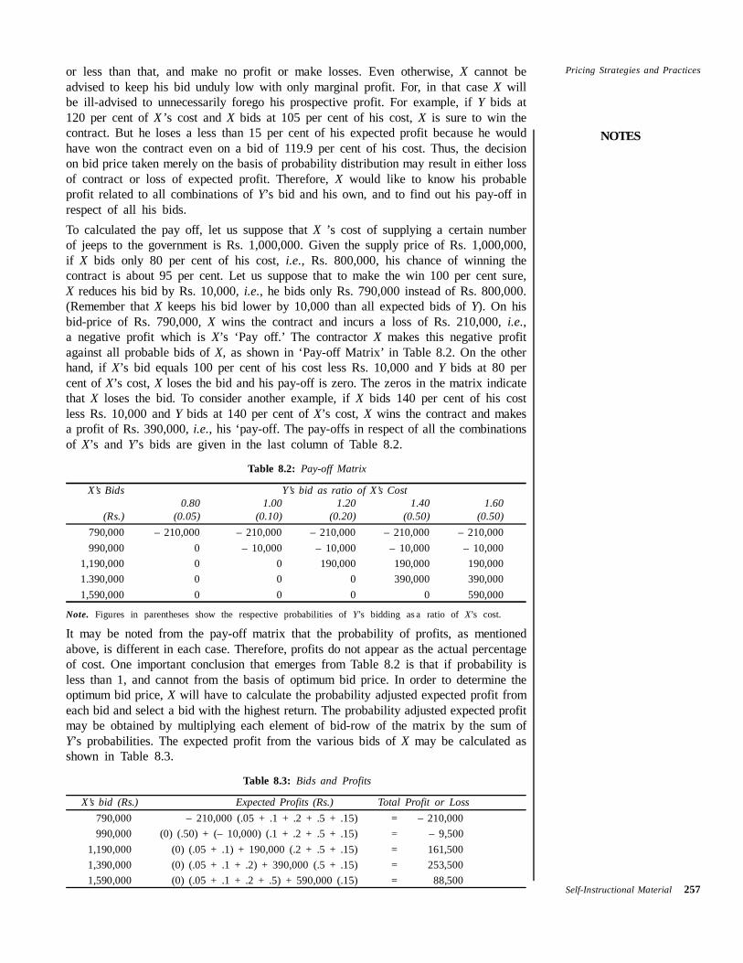
Pricing Strategies and Practicesor less than that, and make no profit or make losses. Even otherwise, X cannot beadvised to keep his bid unduly low with only marginal profit. For, in that case X willbe ill-advised to unnecessarily forego his prospective profit. For example, if Y bids at120 per cent of X ’s cost and X bids at 105 per cent of his cost, X is sure to win thecontract. But he loses a less than 15 per cent of his expected profit because he wouldhave won the contract even on a bid of 119.9 per cent of his cost. Thus, the decisionon bid price taken merely on the basis of probability distribution may result in either lossof contract or loss of expected profit. Therefore, X would like to know his probableprofit related to all combinations of Y’s bid and his own, and to find out his pay-off inrespect of all his bids.To calculated the pay off, let us suppose that X ’s cost of supplying a certain numberof jeeps to the government is Rs. 1,000,000. Given the supply price of Rs. 1,000,000,if X bids only 80 per cent of his cost, i.e., Rs. 800,000, his chance of winning thecontract is about 95 per cent. Let us suppose that to make the win 100 per cent sure,X reduces his bid by Rs. 10,000, i.e., he bids only Rs. 790,000 instead of Rs. 800,000.(Remember that X keeps his bid lower by 10,000 than all expected bids of Y). On hisbid-price of Rs. 790,000, X wins the contract and incurs a loss of Rs. 210,000, i.e.,a negative profit which is X’s ‘Pay off.’ The contractor X makes this negative profitagainst all probable bids of X, as shown in ‘Pay-off Matrix’ in Table 8.2. On the otherhand, if X’s bid equals 100 per cent of his cost less Rs. 10,000 and Y bids at 80 percent of X’s cost, X loses the bid and his pay-off is zero. The zeros in the matrix indicatethat X loses the bid. To consider another example, if X bids 140 per cent of his costless Rs. 10,000 and Y bids at 140 per cent of X’s cost, X wins the contract and makesa profit of Rs. 390,000, i.e., his ‘pay-off. The pay-offs in respect of all the combinationsof X’s and Y’s bids are given in the last column of Table 8.2.

Table 8.2: Pay-off Matrix

X’s Bids Y’s bid as ratio of X’s Cost0.80 1.00 1.20 1.40 1.60

(Rs.) (0.05) (0.10) (0.20) (0.50) (0.50)790,000 – 210,000 – 210,000 – 210,000 – 210,000 – 210,000990,000 0 – 10,000 – 10,000 – 10,000 – 10,000

1,190,000 0 0 190,000 190,000 190,0001.390,000 0 0 0 390,000 390,0001,590,000 0 0 0 0 590,000

Note. Figures in parentheses show the respective probabilities of Y’s bidding as a ratio of X’s cost.

It may be noted from the pay-off matrix that the probability of profits, as mentionedabove, is different in each case. Therefore, profits do not appear as the actual percentageof cost. One important conclusion that emerges from Table 8.2 is that if probability isless than 1, and cannot from the basis of optimum bid price. In order to determine theoptimum bid price, X will have to calculate the probability adjusted expected profit fromeach bid and select a bid with the highest return. The probability adjusted expected profitmay be obtained by multiplying each element of bid-row of the matrix by the sum ofY’s probabilities. The expected profit from the various bids of X may be calculated asshown in Table 8.3.

Table 8.3: Bids and Profits

X’s bid (Rs.) Expected Profits (Rs.) Total Profit or Loss790,000 – 210,000 (.05 + .1 + .2 + .5 + .15) = – 210,000990,000 (0) (.50) + (– 10,000) (.1 + .2 + .5 + .15) = – 9,500

1,190,000 (0) (.05 + .1) + 190,000 (.2 + .5 + .15) = 161,5001,390,000 (0) (.05 + .1 + .2) + 390,000 (.5 + .15) = 253,5001,590,000 (0) (.05 + .1 + .2 + .5) + 590,000 (.15) = 88,500

NOTES


Pricing Strategies and Practices It may be noted from the Table 8.3 that the probability adjusted (expected) profit ismaximum when X’s bid price is Rs. 1,390,000. If X bids Rs. 1,390,000 there is greatpossibility that X wins the contract for supplying jeeps to the government.

8.8 PEAK LOAD PRICING

There are certain non-storable goods, e.g., electricity, telephones etc., which aredemanded in varying amounts in day and night times. Consumption of electricity reachesits peak in day time. It is called ‘peak-load’ time. It reaches its bottom in the night. Thisis called ‘off-peak’ time. Electricity consumption peaks in daytime because all businessestablishments, offices and factories come into operation. It decreases during nightsbecause most business establishments are closed and household consumption falls to itsbasic minimum. Also, in India, demand for electricity peaks during summers due to useof ACs and coolers, and it declines to its minimum level during winters. Similarly,consumption of telephone services is at its peak at day time and at its bottom at nights.Another example of ‘peak’ and ‘off-peak’ demand is of railway services. During festivalsand summer holidays, ‘Pooja’ vacations, the demand for railway travel services rises toits peak.A technical feature of such products is that they cannot be stored. Therefore, theirproduction has to be increased in order to meet the ‘peak-load’ demand and reduced to‘off-peak’ level when demand decreases. Had they been storable, the excess productionin ‘off-peak’ period could be stored and supplied during the ‘peak-load’ period. But thiscannot be done. Besides, given the installed capacity, their production can be increasedbut at an increasing marginal cost (MC).

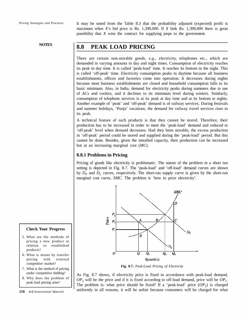
8.8.1 Problems in PricingPricing of goods like electricity is problematic. The nature of the problem in a short runsetting is depicted in Fig. 8.7. The ‘peak-load’ and ‘off-load’ demand curves are shownby DP and DL curves, respectively. The short-run supply curve is given by the short-runmarginal cost curve, SMC. The problem is ‘how to price electricity’.

Fig. 8.7: Peak-Load Pricing of Electricity

As Fig. 8.7 shows, if electricity price is fixed in accordance with peak-load demand,OP3 will be the price and if it is fixed according to off-load demand, price will be OP1.The problem is: what price should be fixed? If a ‘peak-load’ price (OP3) is chargeduniformly in all reasons, it will be unfair because consumers will be charged for what

Check Your Progress

5. What are the methods ofpricing a new product inrelation to establishedproducts?

6. What is meant by transferpricing with externalcompetitive market?

7. What is the method of pricingunder competitive bidding?

8. Why does the problem ofpeak load pricing arise?

NOTES


Pricing Strategies and Practicesthey do not consume. Besides, it may affect business activities adversely. If electricityproduction is a public monopoly, the government will not allow a uniform ‘peak-load’price.On the other hand, if a uniform ‘off load’ price (OP1) is charged, production will fallto OQ2 and there will be acute shortage of electricity during peak hours. It leads to‘breakdowns’ and ‘load-shedding’ during peak-load periods, which disrupt productionand make life miserable. This is a regular feature in Delhi, the capital city of India. Thisis because electricity rates in Delhi are said to be one of the lowest in the country.Alternatively, if an average of the two prices, say P2 is charged, it will have the demeritsof both ‘peak-load’ and ‘off-load’ prices. There will be an excess production to theextent of AB during the ‘off-load’ period, which will go waste as it cannot be stored.If production is restricted to OQ1, price P2 will be unfair. And, during the “peak-load”period, there will be a shortage to the extent of BC, which can be produced only at anextra marginal cost of CD.

8.8.2 Double Pricing SystemFor the above reasons, generally, a double pricing system is adopted. A higher price,called ‘peak-load price’ (OP3) is charged during the ‘peak-load’ period and a lower price(OP1) is charged during the ‘off–peak’ period. During the ‘peak-load’ period, productionis increased to OQ3 at which DP intersects SMC, and production is reduced to OQ1during the ‘off-peak’ period.Advantages Peak-load pricing system has two advantages.(i) It results in an efficient distribution of electricity consumption. Housewives run their

dishwashers and washing machines during the ‘off-peak’ period.(ii) It helps in preventing a loss to the electricity company and ensures regular supply

of electricity in the long run.Disadvantages This system has two disadvantages too.(i) The businesses which are by nature day-business pay higher rates than those which

can be shifted to ‘off-peak’ period.(ii) Billing system is the greatest problem. Each consumer will have to install two

meters—one for ‘peak-load’ and another for ‘off-load’ period with an automaticswitch-over system. This can be done.Alternatively, the problem can be resolved by adopting a progressive tariff rate for the

use of electricity. But, in a country like India, all pervasive corruption will make itinefficient. Delhi Vidyut Board (DVB) is reportedly able to collect only about 50% of itscost of production. The rest goes to the unauthorized users of electricity.

8.9 SUMMARY

Some economists have challenged the conventional theory of pricing. Besides,there are certain conditions under which theoretical pricing method cannot beapplied. Therefore firms adopt different methods of and rules of pricing. Somepricing practices are discussed here briefly.A common practice of pricing a product is ‘cost-plus pricing’ method. Under thismethod price of a product is determined on the basic of a formula, i.e., P = AVC+ AVC (m), where m is profit margin as percentage of average variable cost (AVC).In case a firm produces multiple brands of a product, it follows the traditionaltheoretical rule, i.e., the profit maximization rule for each product a different demandcurve.

NOTES


Pricing Strategies and Practices Different methods are used in pricing a product over the period of its life cycle—introduction, growth, a penetration price policy is adopted at the introduction stageand skimming price policy later when there is no close substitute.In case of pricing a new product in relation to established products, three kinds ofpricing policies are used depending on market conditions (i) pricing below themarket price, (ii) pricing at market price, and (iii) pricing above the market price.Similarly different methods are used in pricing a product used by the firm itself,called transfer pricing; pricing a product under competitive bidding, and pricing aproduct whose demand varies seasonally like electricity.

8.10 ANSWERS TO ‘CHECK YOUR PROGRESS’

1. The formula for cost-plus pricing is given as Price (P) = AVC + AVC (m), wherem is profit margin of average variable cost (AVC).

2. Cost plus pricing is not much different from margined rule pricing. By using therelationship between price (P) and MR, it can be shown that both the methods ofclose to one another.

3. Pricing different products of a multiple product firm is the same as the marginalrule of pricing. Equilibrium output of each product is determined where itsMC = MR. One output is determined, the price of a determined automatically givenits demand curve.

4. The life cycle of a product has five stages: (i) Introduction, (ii) Growth,(iii) Maturity, and (iv) Saturation, and (v) Decline.

5. Depending on the market conditions, three methods are generally used in pricing anew product in relation to established ones, viz., (i) pricing below the market pricefor capturing a market share, (ii) pricing at par with market price if purpose is toavoid competition and to show comparable quality, and (iii) pricing above themarket price, especially in case of luxury goods sold in prestigious malls.

6. In case of competitive external market, market demand for the product of asubsidiary is considered to be a straight horizontal line and AR = MR. In that caseprice is determined at a point where MC curve of its subsidiary interacts the demandcurve.

7. Given the objective of the bidding firm-whether or not to win-pricing is done onthe basis of past experience and the probability rate of winning the bid.

8. Problem of peak load pricing arises because of variation in demand for a product(e.g., electricity) from season to season between low and peak demand. Here theproblem is how to find the average seasonal price.

8.11 EXERCISES AND QUESTIONS

1. Discuss the controversy between marginal theorists and the empiricists on therelevance of ‘marginal rule’ in pricing the products by the manufacturing firms.

2. Describe mark-up pricing and show that mark-up pricing is based on ‘marginalrule’.

3. Distinguish between skimming price and penetration price policy. Which of thesepolicies is relevant in pricing a new product under different competitive conditionsin the market?

4. What is transfer pricing? How is transfer price determined if (i) there is no externalmarket for the transfer product, and (ii) there is an external market for it?

NOTES


Pricing Strategies and Practices5. What is competitive bidding? Describe the technique of competitive bidding of priceunder the condition of uncertainty.

6. What kind of pricing strategy is adopted over the life-cycle of a product. What doyou think will be an appropriate price policy when the demand reaches its saturationand substitute products are likely to enter the market?

7. Discuss the technique of multiple product pricing. Illustrate your answer. Why can’ta single average price be fixed for all products?

8. What is meant by ‘peak-load pricing’? Why is sometimes peak-load pricinginevitable? What are its advantages and disadvantages?

8.12 FURTHER READING

Brigham, Eugene, F. and James L. Pappas, Managerial Economics, 3rd Edn., DrydenPress, Hinsdale, III, 1979, Ch. 11.Douglas, Evan J., Managerial Economics: Theory, Proactice and Problem, Prentice HallInc., N.J., 1979, Ch. 11.Koutsoyiannis, A., Modern Microeconomics, Macmillan Press Ltd., 1979, Ch. 11.Spencer Milton H., Managerial Economics, Richard D, Irwin, III, 1968. Ch. 11.Webb, Samuel, C., Managerial Economics, Houghton Miffln, Boston, 1976, Ch. 8.

References1. The ‘fair’ percentage of profit margin is usually determined on the basis of the

firm’s past experience and the practice of the rival firms.2. A. Silbertson, “Price Behaviour of Firms”, Economic Journal, September, 1970.3 . For Example, the different models of Maruti automobiles, viz., Maruti 800, Zen,

Maruti 1000, Esteem, Maruti Van and Wagon-R, etc.4. E.W. Clemens, ‘Price Discrimination and Multiple Product Firm’, Review of Eco-

nomic Studies (1950–51). Reprinted in Industrial Organisation and Public policy(Am. Eco. Assn.) Richard D. Irwin, Illinois, 1959.

5. Managerial Economics., op. cit., p. 425.6. Jack Hirshleifer, “On the Economics of Transfer Pricing” Journal of Business, July,

1956.7. The MRc can also be obtained by asking the compressor division how much it will

supply at different transfer prices. MRr – Tp gives MRc, also known as “marginalnet revenue”.

All rights reserved. No part of this publication which is material protected by this copyright noticemay be reproduced or transmitted or utilized or stored in any form or by any means now known orhereinafter invented, electronic, digital or mechanical, including photocopying, scanning, recordingor by any information storage or retrieval system, without prior written permission from the Publisher.

Information contained in this book has been published by VIKAS® Publishing House Pvt. Ltd. and hasbeen obtaine1d by its Authors from sources believed to be reliable and are correct to the best of theirknowledge. However, the Publisher, its Authors & Mahatma Gandhi University shall in no event beliable for any errors, omissions or damages arising out of use of this information and specificallydisclaim any implied warranties or merchantability or fitness for any particular use.

Vikas® is the registered trademark of Vikas® Publishing House Pvt. Ltd.

VIKAS® PUBLISHING HOUSE PVT LTDE-28, Sector-8, Noida - 201301 (UP)Phone: 0120-4078900 � � Fax: 0120-4078999Regd. Office: 576, Masjid Road, Jangpura, New Delhi 110 014Website: www.vikaspublishing.com � Email: [email protected]

UBS The Sampuran Prakash School of Executive EducationGurgaon, Haryana, Indiawww.ubs.edu.in

Copyright © Author, 2010

Documents

UNIT 8 PRICING STRATEGIES AND PRACTICES …application.dbuglobal.com/assets/Pu18ME1002/CPu18ME1002...NOTES Self-Instructional Material 243 Pricing Strategies and Practices UNIT 8 PRICING