Unit ed Sta te s E n v ironment al P rot ect ion IE NSC

SCIENCE

United StatesEnvironmental ProtectionAgency

EPA 600/R-08/041B | September 2012 | www.epa.gov/ord

User’s Manual TEVA-SPOT ToolkitVERSION 2.5.2

Office of Research and DevelopmentNational Homeland Security Research Center

Printed Sep 2012

User's Manual

TEVA-SPOT Toolkit 2.5.2

by

Jonathan Berry, Erik Boman, Lee Ann Riesen

Scalable Algorithms Dept

Sandia National Laboratories

Albuquerque, NM 87185

William E. Hart, Cynthia A. Phillips, Jean-Paul Watson

Discrete Math and Complex Systems Dept


Albuquerque, NM 87185

Project O�cer:

Regan Murray

National Homeland Security Research Center

Office of Research and Development

U.S. Environmental Protection Agency

Cincinnati, OH 45256

2

The U.S. Environmental Protection Agency (EPA) through its Office of Research and Develop-ment funded and collaborated in the research described here under an Inter-Agency Agreementwith the Department of Energy’s Sandia National Laboratories (IAG # DW8992192801). Thisdocument has been subjected to the Agency’s review, and has been approved for publication asan EPA document. EPA does not endorse the purchase or sale of any commercial products orservices.

NOTICE: This report was prepared as an account of work sponsored by an agency of the UnitedStates Government. Accordingly, the United States Government retains a nonexclusive, royalty-free license to publish or reproduce the published form of this contribution, or allow others todo so for United States Government purposes. Neither Sandia Corporation, the United StatesGovernment, nor any agency thereof, nor any of their employees makes any warranty, expressor implied, or assumes any legal liability or responsibility for the accuracy, completeness, orusefulness of any information, apparatus, product, or process disclosed, or represents that its usewould not infringe privately-owned rights. Reference herein to any specific commercial product,process, or service by trade name, trademark, manufacturer, or otherwise does not necessarilyconstitute or imply its endorsement, recommendation, or favoring by Sandia Corporation, theUnited States Government, or any agency thereof. The views and opinions expressed herein donot necessarily state or reflect those of Sandia Corporation, the United States Government orany agency thereof.

Questions concerning this document or its application should be addressed to:

Regan MurrayUSEPA/NHSRC (NG 16)26 W Martin Luther King DriveCincinnati OH 45268(513) [email protected]

Sandia is a multiprogram laboratory operated by Sandia Corpora-tion, a Lockheed Martin Company, for the United States Depart-ment of Energy's National Nuclear Security Administration underContract DE-AC04-94-AL85000.

3

Forward

Since its inception in 1970, EPA's mission has been to pursue a cleaner, healthier environment for theAmerican people. The Agency was assigned the daunting task of repairing the damage already done tothe natural environment and establishing new criteria to guide Americans in making a cleaner environmenta reality. Since 1970, the EPA has worked with federal, state, tribal, and local partners to advance itsmission to protect human health and the environment. In order to carry out its mission, EPA employs andcollaborates with some of the nation's best scienti�c minds. EPA prides itself in applying sound science andstate of the art techniques and methods to develop and test innovations that will protect both human healthand the environment.

Under existing laws and recent Homeland Security Presidential Directives, EPA has been called upon to playa vital role in helping to secure the nation against foreign and domestic enemies. The National HomelandSecurity Research Center (NHSRC) was formed in 2002 to conduct research in support of EPA's role inhomeland security. NHSRC research e�orts focus on �ve areas: water infrastructure protection, threat andconsequence assessment, decontamination and consequence management, response capability enhancement,and homeland security technology testing and evaluation. EPA is the lead federal agency for drinking waterand wastewater systems and the NHSRC is working to reduce system vulnerabilities, prevent and prepare forterrorist attacks, minimize public health impacts and infrastructure damage, and enhance recovery e�orts.

This Users Manual for the TEVA-SPOT Toolkit software package is published and made available by EPA'sO�ce of Research and Development to assist the user community and to link researchers with their clients.

Jonathan Herrmann, Director

National Homeland Security Research CenterO�ce of Research and DevelopmentU. S. Environmental Protection Agency

4

License Notice

TEVA-SPOT Toolkit is Copyright 2008 Sandia Corporation. Under the terms of Contract DE-AC04-94AL85000 with Sandia Corporation, the U.S. Government retains certain rights in this software.

The �library� refers to the TEVA-SPOT Toolkit software, both the executable and associated source code.This library is free software; you can redistribute it and/or modify it under the terms of the BSD License aspublished by the Free Software Foundation.

This library is distributed in the hope that it will be useful, but WITHOUT ANY WARRANTY; withouteven the implied warranty of MERCHANTABILITY or FITNESS FOR A PARTICULAR PURPOSE. Seethe GNU Lesser General Public License for more details.

The TEVA-SPOT Toolkit utilizes a variety of external executables that are distributed under separateopen-source licenses:

• PICO - BSD and Common Public License

• randomsample, sideconstraints - ATT Software for noncommercial use.

• u� - Common Public License

5

Acknowledgements

The National Homeland Security Research Center would like to acknowledge the following organizations andindividuals for their support in the development of the TEVA-SPOT Toolkit User's Manual and/or in thedevelopment and testing of the TEVA-SPOT Toolkit Software.

O�ce of Research and Development - National Homeland Security Research Center

Robert JankeRegan MurrayTerra Haxton


Jonathan BerryErik BomanWilliam HartLee Ann RiesenCynthia PhillipsJean-Paul WatsonDavid HartKatherine Klise

Argonne National Laboratory

Thomas Taxon

University of Cincinnati

James Uber

American Water Works Association Utility Users Group

Kevin Morley

6

Contents

1 Introduction 1

1.1 What is TEVA-SPOT? . . . . . . . . . . . . . . . . . . . . . . . . . . . . . . . . . . . . . . . . . . . . . . . . . . . . . . . . . . 1

1.2 About This Manual . . . . . . . . . . . . . . . . . . . . . . . . . . . . . . . . . . . . . . . . . . . . . . . . . . . . . . . . . . . . . 2

2 TEVA-SPOT Toolkit Basics 3

2.1 Approaches to Sensor Placement . . . . . . . . . . . . . . . . . . . . . . . . . . . . . . . . . . . . . . . . . . . . . . . . . . 3

2.2 The Main Steps in Using SPOT . . . . . . . . . . . . . . . . . . . . . . . . . . . . . . . . . . . . . . . . . . . . . . . . . . . 4

2.2.1 Simulating Contamination Incidents . . . . . . . . . . . . . . . . . . . . . . . . . . . . . . . . . . . . . . . . . 4

2.2.2 Computing Contamination Impacts . . . . . . . . . . . . . . . . . . . . . . . . . . . . . . . . . . . . . . . . . . 4

2.2.3 Performing Sensor Placement . . . . . . . . . . . . . . . . . . . . . . . . . . . . . . . . . . . . . . . . . . . . . . . 5

2.2.4 Evaluating a Sensor Placement . . . . . . . . . . . . . . . . . . . . . . . . . . . . . . . . . . . . . . . . . . . . . . 5

2.3 Installation and Requirements for Using SPOT . . . . . . . . . . . . . . . . . . . . . . . . . . . . . . . . . . . . . . 6

2.4 Reporting Bugs and Feature Requests . . . . . . . . . . . . . . . . . . . . . . . . . . . . . . . . . . . . . . . . . . . . . . 7

3 Sensor Placement Formulations 8

3.1 The Standard SPOT Formulation . . . . . . . . . . . . . . . . . . . . . . . . . . . . . . . . . . . . . . . . . . . . . . . . . 8

3.2 Robust SPOT Formulations . . . . . . . . . . . . . . . . . . . . . . . . . . . . . . . . . . . . . . . . . . . . . . . . . . . . . . 9

3.3 Min-Cost Formulations . . . . . . . . . . . . . . . . . . . . . . . . . . . . . . . . . . . . . . . . . . . . . . . . . . . . . . . . . . 10

3.4 Formulations with Multiple Objectives . . . . . . . . . . . . . . . . . . . . . . . . . . . . . . . . . . . . . . . . . . . . . 10

3.5 The SPOT Formulation with Imperfect Sensors . . . . . . . . . . . . . . . . . . . . . . . . . . . . . . . . . . . . . . 11

4 Contamination Incidents and Impact Measures 12

4.1 Simulating Contamination Incidents . . . . . . . . . . . . . . . . . . . . . . . . . . . . . . . . . . . . . . . . . . . . . . . 12

4.2 Using tso2Impact . . . . . . . . . . . . . . . . . . . . . . . . . . . . . . . . . . . . . . . . . . . . . . . . . . . . . . . . . . . . . . . 12

4.3 Impact Measures . . . . . . . . . . . . . . . . . . . . . . . . . . . . . . . . . . . . . . . . . . . . . . . . . . . . . . . . . . . . . . . 13

4.4 Advanced Tools for Large Sensor Placements Problems . . . . . . . . . . . . . . . . . . . . . . . . . . . . . . . . 15

5 Sensor Placement Solvers 16

5.1 A Simple Example . . . . . . . . . . . . . . . . . . . . . . . . . . . . . . . . . . . . . . . . . . . . . . . . . . . . . . . . . . . . . . 16

5.2 Computing a Bound on the Best Sensor Placement Value . . . . . . . . . . . . . . . . . . . . . . . . . . . . . . 20

7

5.3 Minimizing the Number of Sensors . . . . . . . . . . . . . . . . . . . . . . . . . . . . . . . . . . . . . . . . . . . . . . . . . 20

5.4 Fixing Sensor Placement Locations . . . . . . . . . . . . . . . . . . . . . . . . . . . . . . . . . . . . . . . . . . . . . . . . 21

5.5 Robust Optimization of Sensor Locations . . . . . . . . . . . . . . . . . . . . . . . . . . . . . . . . . . . . . . . . . . . 22

5.6 Multi-Criteria Analysis . . . . . . . . . . . . . . . . . . . . . . . . . . . . . . . . . . . . . . . . . . . . . . . . . . . . . . . . . . 23

5.7 Sensor Placements without Penalties . . . . . . . . . . . . . . . . . . . . . . . . . . . . . . . . . . . . . . . . . . . . . . . 26

5.8 Limited-Memory Sensor Placement Techniques . . . . . . . . . . . . . . . . . . . . . . . . . . . . . . . . . . . . . . . 28

5.9 Two-tiered Sensor Placement Approach . . . . . . . . . . . . . . . . . . . . . . . . . . . . . . . . . . . . . . . . . . . . . 29

5.10 Evaluating a Sensor Placement . . . . . . . . . . . . . . . . . . . . . . . . . . . . . . . . . . . . . . . . . . . . . . . . . . . . 30

5.11 Sensor Placement with Imperfect Sensors . . . . . . . . . . . . . . . . . . . . . . . . . . . . . . . . . . . . . . . . . . . 32

5.12 Summary of Solver Features . . . . . . . . . . . . . . . . . . . . . . . . . . . . . . . . . . . . . . . . . . . . . . . . . . . . . . 33

6 File Formats 35

6.1 TSG File . . . . . . . . . . . . . . . . . . . . . . . . . . . . . . . . . . . . . . . . . . . . . . . . . . . . . . . . . . . . . . . . . . . . . . 35

6.2 TSI File . . . . . . . . . . . . . . . . . . . . . . . . . . . . . . . . . . . . . . . . . . . . . . . . . . . . . . . . . . . . . . . . . . . . . . 36

6.3 DVF File . . . . . . . . . . . . . . . . . . . . . . . . . . . . . . . . . . . . . . . . . . . . . . . . . . . . . . . . . . . . . . . . . . . . . . 36

6.4 TAI File . . . . . . . . . . . . . . . . . . . . . . . . . . . . . . . . . . . . . . . . . . . . . . . . . . . . . . . . . . . . . . . . . . . . . . 37

6.5 ERD File . . . . . . . . . . . . . . . . . . . . . . . . . . . . . . . . . . . . . . . . . . . . . . . . . . . . . . . . . . . . . . . . . . . . . 39

6.6 Sensor Placement File . . . . . . . . . . . . . . . . . . . . . . . . . . . . . . . . . . . . . . . . . . . . . . . . . . . . . . . . . . . 39

6.7 Impact File . . . . . . . . . . . . . . . . . . . . . . . . . . . . . . . . . . . . . . . . . . . . . . . . . . . . . . . . . . . . . . . . . . . . 40

6.8 LAG File . . . . . . . . . . . . . . . . . . . . . . . . . . . . . . . . . . . . . . . . . . . . . . . . . . . . . . . . . . . . . . . . . . . . . . 40

6.9 Scenario File . . . . . . . . . . . . . . . . . . . . . . . . . . . . . . . . . . . . . . . . . . . . . . . . . . . . . . . . . . . . . . . . . . . 41

6.10 Node File . . . . . . . . . . . . . . . . . . . . . . . . . . . . . . . . . . . . . . . . . . . . . . . . . . . . . . . . . . . . . . . . . . . . . 41

6.11 Sensor Placement Con�guration File . . . . . . . . . . . . . . . . . . . . . . . . . . . . . . . . . . . . . . . . . . . . . . . 41

6.12 Sensor Placement Costs File . . . . . . . . . . . . . . . . . . . . . . . . . . . . . . . . . . . . . . . . . . . . . . . . . . . . . . 42

6.13 Placement Locations File . . . . . . . . . . . . . . . . . . . . . . . . . . . . . . . . . . . . . . . . . . . . . . . . . . . . . . . . 42

6.14 Sensor Class File . . . . . . . . . . . . . . . . . . . . . . . . . . . . . . . . . . . . . . . . . . . . . . . . . . . . . . . . . . . . . . . 43

6.15 Junctions Class File . . . . . . . . . . . . . . . . . . . . . . . . . . . . . . . . . . . . . . . . . . . . . . . . . . . . . . . . . . . . . 43

Appendix

A Unix Installation 47

A.1 Downloading . . . . . . . . . . . . . . . . . . . . . . . . . . . . . . . . . . . . . . . . . . . . . . . . . . . . . . . . . . . . . . . . . . . 47

A.2 Con�guring and Building . . . . . . . . . . . . . . . . . . . . . . . . . . . . . . . . . . . . . . . . . . . . . . . . . . . . . . . . 47

8

B Data Requirements 48

C Executable evalsensor 57

C.1 Overview . . . . . . . . . . . . . . . . . . . . . . . . . . . . . . . . . . . . . . . . . . . . . . . . . . . . . . . . . . . . . . . . . . . . . . 57

C.2 Command-Line Help . . . . . . . . . . . . . . . . . . . . . . . . . . . . . . . . . . . . . . . . . . . . . . . . . . . . . . . . . . . . 57

C.3 Description . . . . . . . . . . . . . . . . . . . . . . . . . . . . . . . . . . . . . . . . . . . . . . . . . . . . . . . . . . . . . . . . . . . . 58

D Executable �lter_impacts 59

D.1 Overview . . . . . . . . . . . . . . . . . . . . . . . . . . . . . . . . . . . . . . . . . . . . . . . . . . . . . . . . . . . . . . . . . . . . . . 59

D.2 Usage . . . . . . . . . . . . . . . . . . . . . . . . . . . . . . . . . . . . . . . . . . . . . . . . . . . . . . . . . . . . . . . . . . . . . . . . 59

D.3 Options . . . . . . . . . . . . . . . . . . . . . . . . . . . . . . . . . . . . . . . . . . . . . . . . . . . . . . . . . . . . . . . . . . . . . . . 59

D.4 Arguments . . . . . . . . . . . . . . . . . . . . . . . . . . . . . . . . . . . . . . . . . . . . . . . . . . . . . . . . . . . . . . . . . . . . 59

D.5 Description . . . . . . . . . . . . . . . . . . . . . . . . . . . . . . . . . . . . . . . . . . . . . . . . . . . . . . . . . . . . . . . . . . . . 59

D.6 Notes . . . . . . . . . . . . . . . . . . . . . . . . . . . . . . . . . . . . . . . . . . . . . . . . . . . . . . . . . . . . . . . . . . . . . . . . . 59

E Executable PICO 60

E.1 Overview . . . . . . . . . . . . . . . . . . . . . . . . . . . . . . . . . . . . . . . . . . . . . . . . . . . . . . . . . . . . . . . . . . . . . . 60

E.2 Usage . . . . . . . . . . . . . . . . . . . . . . . . . . . . . . . . . . . . . . . . . . . . . . . . . . . . . . . . . . . . . . . . . . . . . . . . 60

E.3 Options . . . . . . . . . . . . . . . . . . . . . . . . . . . . . . . . . . . . . . . . . . . . . . . . . . . . . . . . . . . . . . . . . . . . . . . 60

E.4 Description . . . . . . . . . . . . . . . . . . . . . . . . . . . . . . . . . . . . . . . . . . . . . . . . . . . . . . . . . . . . . . . . . . . . 60

E.5 Notes . . . . . . . . . . . . . . . . . . . . . . . . . . . . . . . . . . . . . . . . . . . . . . . . . . . . . . . . . . . . . . . . . . . . . . . . . 60

F Executable randomsample 61

F.1 Overview . . . . . . . . . . . . . . . . . . . . . . . . . . . . . . . . . . . . . . . . . . . . . . . . . . . . . . . . . . . . . . . . . . . . . . 61

F.2 Usage . . . . . . . . . . . . . . . . . . . . . . . . . . . . . . . . . . . . . . . . . . . . . . . . . . . . . . . . . . . . . . . . . . . . . . . . 61

F.3 Arguments . . . . . . . . . . . . . . . . . . . . . . . . . . . . . . . . . . . . . . . . . . . . . . . . . . . . . . . . . . . . . . . . . . . . 61

F.4 Description . . . . . . . . . . . . . . . . . . . . . . . . . . . . . . . . . . . . . . . . . . . . . . . . . . . . . . . . . . . . . . . . . . . . 61

F.5 Notes . . . . . . . . . . . . . . . . . . . . . . . . . . . . . . . . . . . . . . . . . . . . . . . . . . . . . . . . . . . . . . . . . . . . . . . . . 61

G Executable scenarioAggr 62

G.1 Overview . . . . . . . . . . . . . . . . . . . . . . . . . . . . . . . . . . . . . . . . . . . . . . . . . . . . . . . . . . . . . . . . . . . . . . 62

G.2 Usage . . . . . . . . . . . . . . . . . . . . . . . . . . . . . . . . . . . . . . . . . . . . . . . . . . . . . . . . . . . . . . . . . . . . . . . . 62

G.3 Options . . . . . . . . . . . . . . . . . . . . . . . . . . . . . . . . . . . . . . . . . . . . . . . . . . . . . . . . . . . . . . . . . . . . . . . 62

G.4 Description . . . . . . . . . . . . . . . . . . . . . . . . . . . . . . . . . . . . . . . . . . . . . . . . . . . . . . . . . . . . . . . . . . . . 62

9

G.5 Notes . . . . . . . . . . . . . . . . . . . . . . . . . . . . . . . . . . . . . . . . . . . . . . . . . . . . . . . . . . . . . . . . . . . . . . . . . 62

H Executable createIPData 63

H.1 Overview . . . . . . . . . . . . . . . . . . . . . . . . . . . . . . . . . . . . . . . . . . . . . . . . . . . . . . . . . . . . . . . . . . . . . . 63

H.2 Command-Line Help . . . . . . . . . . . . . . . . . . . . . . . . . . . . . . . . . . . . . . . . . . . . . . . . . . . . . . . . . . . . 63

H.3 Description . . . . . . . . . . . . . . . . . . . . . . . . . . . . . . . . . . . . . . . . . . . . . . . . . . . . . . . . . . . . . . . . . . . . 63

H.4 Notes . . . . . . . . . . . . . . . . . . . . . . . . . . . . . . . . . . . . . . . . . . . . . . . . . . . . . . . . . . . . . . . . . . . . . . . . . 63

I Executable sideconstraints 64

I.1 Overview . . . . . . . . . . . . . . . . . . . . . . . . . . . . . . . . . . . . . . . . . . . . . . . . . . . . . . . . . . . . . . . . . . . . . . 64

I.2 Usage . . . . . . . . . . . . . . . . . . . . . . . . . . . . . . . . . . . . . . . . . . . . . . . . . . . . . . . . . . . . . . . . . . . . . . . . 64

I.3 Arguments . . . . . . . . . . . . . . . . . . . . . . . . . . . . . . . . . . . . . . . . . . . . . . . . . . . . . . . . . . . . . . . . . . . . 64

I.4 Description . . . . . . . . . . . . . . . . . . . . . . . . . . . . . . . . . . . . . . . . . . . . . . . . . . . . . . . . . . . . . . . . . . . . 64

J Executable sp 65

J.1 Overview . . . . . . . . . . . . . . . . . . . . . . . . . . . . . . . . . . . . . . . . . . . . . . . . . . . . . . . . . . . . . . . . . . . . . . 65

J.2 Command-Line Help . . . . . . . . . . . . . . . . . . . . . . . . . . . . . . . . . . . . . . . . . . . . . . . . . . . . . . . . . . . . 65

J.3 Description . . . . . . . . . . . . . . . . . . . . . . . . . . . . . . . . . . . . . . . . . . . . . . . . . . . . . . . . . . . . . . . . . . . . 68

J.4 Notes . . . . . . . . . . . . . . . . . . . . . . . . . . . . . . . . . . . . . . . . . . . . . . . . . . . . . . . . . . . . . . . . . . . . . . . . . 69

K Executable sp-2tier 70

K.1 Overview . . . . . . . . . . . . . . . . . . . . . . . . . . . . . . . . . . . . . . . . . . . . . . . . . . . . . . . . . . . . . . . . . . . . . . 70

K.2 Command-Line Help . . . . . . . . . . . . . . . . . . . . . . . . . . . . . . . . . . . . . . . . . . . . . . . . . . . . . . . . . . . . 70

K.3 Description . . . . . . . . . . . . . . . . . . . . . . . . . . . . . . . . . . . . . . . . . . . . . . . . . . . . . . . . . . . . . . . . . . . . 71

K.4 Notes . . . . . . . . . . . . . . . . . . . . . . . . . . . . . . . . . . . . . . . . . . . . . . . . . . . . . . . . . . . . . . . . . . . . . . . . . 72

L Executable spotSkeleton 73

L.1 Overview . . . . . . . . . . . . . . . . . . . . . . . . . . . . . . . . . . . . . . . . . . . . . . . . . . . . . . . . . . . . . . . . . . . . . . 73

L.2 Usage . . . . . . . . . . . . . . . . . . . . . . . . . . . . . . . . . . . . . . . . . . . . . . . . . . . . . . . . . . . . . . . . . . . . . . . . 73

L.3 Description . . . . . . . . . . . . . . . . . . . . . . . . . . . . . . . . . . . . . . . . . . . . . . . . . . . . . . . . . . . . . . . . . . . . 73

L.4 Notes . . . . . . . . . . . . . . . . . . . . . . . . . . . . . . . . . . . . . . . . . . . . . . . . . . . . . . . . . . . . . . . . . . . . . . . . . 73

M Executable tevasim 75

M.1 Overview . . . . . . . . . . . . . . . . . . . . . . . . . . . . . . . . . . . . . . . . . . . . . . . . . . . . . . . . . . . . . . . . . . . . . . 75

M.2 Command-Line Help . . . . . . . . . . . . . . . . . . . . . . . . . . . . . . . . . . . . . . . . . . . . . . . . . . . . . . . . . . . . 75

10

N Executable tso2Impact 76

N.1 Overview . . . . . . . . . . . . . . . . . . . . . . . . . . . . . . . . . . . . . . . . . . . . . . . . . . . . . . . . . . . . . . . . . . . . . . 76

N.2 Command-Line Help . . . . . . . . . . . . . . . . . . . . . . . . . . . . . . . . . . . . . . . . . . . . . . . . . . . . . . . . . . . . 76

N.3 Description . . . . . . . . . . . . . . . . . . . . . . . . . . . . . . . . . . . . . . . . . . . . . . . . . . . . . . . . . . . . . . . . . . . . 77

N.4 Notes . . . . . . . . . . . . . . . . . . . . . . . . . . . . . . . . . . . . . . . . . . . . . . . . . . . . . . . . . . . . . . . . . . . . . . . . . 77

O Executable u� 78

O.1 Overview . . . . . . . . . . . . . . . . . . . . . . . . . . . . . . . . . . . . . . . . . . . . . . . . . . . . . . . . . . . . . . . . . . . . . . 78

O.2 Usage . . . . . . . . . . . . . . . . . . . . . . . . . . . . . . . . . . . . . . . . . . . . . . . . . . . . . . . . . . . . . . . . . . . . . . . . 78

O.3 Options . . . . . . . . . . . . . . . . . . . . . . . . . . . . . . . . . . . . . . . . . . . . . . . . . . . . . . . . . . . . . . . . . . . . . . . 78

O.4 Arguments . . . . . . . . . . . . . . . . . . . . . . . . . . . . . . . . . . . . . . . . . . . . . . . . . . . . . . . . . . . . . . . . . . . . 78

O.5 Description . . . . . . . . . . . . . . . . . . . . . . . . . . . . . . . . . . . . . . . . . . . . . . . . . . . . . . . . . . . . . . . . . . . . 78

11

12

1 Introduction

Drinking water distribution systems are inherently vulnerable to accidental or intentional contaminationbecause of their distributed geography. Further, there are many challenges to detecting contaminants indrinking water systems: municipal distribution systems are large, consisting of hundreds or thousands ofmiles of pipe; �ow patterns are driven by time-varying demands placed on the system by customers; anddistribution systems are looped, resulting in mixing and dilution of contaminants. The use of on-line,real-time contaminant warning systems (CWSs) is a promising strategy for mitigating these risks. Onlinesensor data can be combined with public health surveillance systems, physical security monitoring, customercomplaint surveillance, and routine sampling programs to e�ect a rapid response to contamination incidents[22].

A variety of technical challenges need to be addressed to make CWSs a practical, reliable element of water se-curity systems. A key aspect of CWS design is the strategic placement of sensors throughout the distributionnetwork. Given a limited number of sensors, a desirable sensor placement minimizes the potential economicand public health impacts of a contaminant incident. There are a wide range of important design objectivesfor sensor placements (e.g., minimizing the cost of sensor installation and maintenance, the response time toa contamination incident, and the extent of contamination). In addition, �exible sensor placement tools areneeded to analyze CWS designs in large scale networks.

1.1 What is TEVA-SPOT?

The Threat Ensemble Vulnerability Assessment and Sensor Placement Optimization Tool (TEVA-SPOT)has been developed by the U. S. Environmental Protection Agency, Sandia National Laboratories, ArgonneNational Laboratory, and the University of Cincinnati. TEVA-SPOT has been used to develop sensor networkdesigns for several large water utilities [12], including the pilot study for EPA's Water Security Initiative.

TEVA-SPOT allows a user to specify a wide range of modeling inputs and performance objectives forcontamination warning system design. Further, TEVA-SPOT supports a �exible decision framework forsensor placement that involves two major steps: a modeling process and a decision-making process [13].The modeling process includes (1) describing sensor characteristics, (2) de�ning the design basis threat, (3)selecting impact measures for the CWS, (4) planning utility response to sensor detection, and (5) identifyingfeasible sensor locations.

The design basis threat for a CWS is the ensemble of contamination incidents that a CWS should bedesigned to protect against. In the simplest case, a design basis threat is a contamination scenario with asingle contaminant that is introduced at a speci�c time and place. Thus, a design basis threat consists ofa set of contamination incidents that can be simulated with standard water distribution system modelingsoftware [18]. TEVA-SPOT provides a convenient interface for de�ning and computing the impacts of designbasis threats. In particular, TEVA-SPOT can simulate many contamination incidents in parallel, which hasreduced the computation of very large design basis threats from weeks to hours on EPA's high performancecomputing system.

TEVA-SPOT was designed to model a wide range of sensor placement problems. For example, TEVA-SPOTsupports a number of impact measures, including the number of people exposed to dangerous levels of acontaminant, the volume of contaminated water used by customers, the number of feet of contaminatedpipe, and the time to detection. Response delays can also be speci�ed to account for the time a water utilitywould need to verify a contamination incident before notifying the public. Finally, the user can specify thefeasible locations for sensors and �x sensor locations during optimization. This �exibility allows a user toevaluate how di�erent factors impact the CWS performance and to iteratively re�ne a CWS design.

1

1.2 About This Manual

The capabilities of TEVA-SPOT can be accessed either with a GUI or from command-line tools. This usermanual describes the TEVA-SPOT Toolkit, which contains these command-line tools. The TEVA-SPOTToolkit can be used within either a MS Windows DOS shell or any standard Unix shell (e.g. the Bash shell).

The following sections describe the TEVA-SPOT Toolkit, which is referred to as SPOT throughout thismanual:

• TEVA-SPOT Toolkit Basics - An introduction to the process of sensor placement, the use of SPOTcommand-line tools, and installation of the SPOT executables.

• Sensor Placement Formulations - The mathematical formulations used by the SPOT solvers.

• Contamination Incidents and Impact Measures - A description of how contamination incidentsare computed, and the impact measures that can be used in SPOT to analyze them.

• Sensor Placement Solvers - A description of how to apply the SPOT sensor placement solvers.

• File Formats - Descriptions of the formats of �les used by the SPOT solvers.

In addition, the appendices of this manual describe the syntax and usage of the SPOT command-line exe-cutables.

2

2 TEVA-SPOT Toolkit Basics

This section provides an introduction to the process of sensor placement, the use of SPOT command-linetools, and the installation of the SPOT executables.

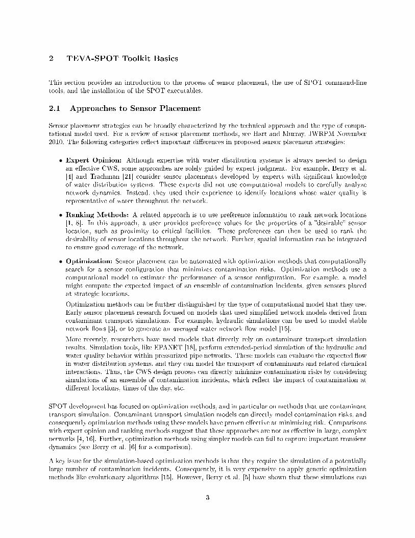
2.1 Approaches to Sensor Placement

Sensor placement strategies can be broadly characterized by the technical approach and the type of compu-tational model used. For a review of sensor placement methods, see Hart and Murray, JWRPM November2010. The following categories re�ect important di�erences in proposed sensor placement strategies:

• Expert Opinion: Although expertise with water distribution systems is always needed to designan e�ective CWS, some approaches are solely guided by expert judgment. For example, Berry et al.[4] and Trachman [21] consider sensor placements developed by experts with signi�cant knowledgeof water distribution systems. These experts did not use computational models to carefully analyzenetwork dynamics. Instead, they used their experience to identify locations whose water quality isrepresentative of water throughout the network.

• Ranking Methods: A related approach is to use preference information to rank network locations[1, 8]. In this approach, a user provides preference values for the properties of a �desirable� sensorlocation, such as proximity to critical facilities. These preferences can then be used to rank thedesirability of sensor locations throughout the network. Further, spatial information can be integratedto ensure good coverage of the network.

• Optimization: Sensor placement can be automated with optimization methods that computationallysearch for a sensor con�guration that minimizes contamination risks. Optimization methods use acomputational model to estimate the performance of a sensor con�guration. For example, a modelmight compute the expected impact of an ensemble of contamination incidents, given sensors placedat strategic locations.

Optimization methods can be further distinguished by the type of computational model that they use.Early sensor placement research focused on models that used simpli�ed network models derived fromcontaminant transport simulations. For example, hydraulic simulations can be used to model stablenetwork �ows [3], or to generate an averaged water network �ow model [15].

More recently, researchers have used models that directly rely on contaminant transport simulationresults. Simulation tools, like EPANET [18], perform extended-period simulation of the hydraulic andwater quality behavior within pressurized pipe networks. These models can evaluate the expected �owin water distribution systems, and they can model the transport of contaminants and related chemicalinteractions. Thus, the CWS design process can directly minimize contamination risks by consideringsimulations of an ensemble of contamination incidents, which re�ect the impact of contamination atdi�erent locations, times of the day, etc.

SPOT development has focused on optimization methods, and in particular on methods that use contaminanttransport simulation. Contaminant transport simulation models can directly model contamination risks, andconsequently optimization methods using these models have proven e�ective at minimizing risk. Comparisonswith expert opinion and ranking methods suggest that these approaches are not as e�ective in large, complexnetworks [4, 16]. Further, optimization methods using simpler models can fail to capture important transientdynamics (see Berry et al. [6] for a comparison).

A key issue for the simulation-based optimization methods is that they require the simulation of a potentiallylarge number of contamination incidents. Consequently, it is very expensive to apply generic optimizationmethods like evolutionary algorithms [15]. However, Berry et al. [5] have shown that these simulations can

3

be performed in an o�-line preprocessing step that is done in advance of the optimization process. Thus, thetime needed for simulation does not necessarily impact the time spent performing sensor placement.

2.2 The Main Steps in Using SPOT

The following example illustrates the main steps required to (1) simulate contamination incidents, (2) com-pute contamination impacts, (3) perform sensor placement, and (4) evaluate a sensor placement. Thisexample places sensors in EPANET Example 3 (Net3), a small distribution system with 97 junctions.

The data �les used in this example are available with the SPOT software package (C:\spot\examples\simpledirectory). Installation instruction are included in Section 2.3 (p. 6). In general, a user will need to usea variety of data sources to develop a sensor placement model. Data requirements for TEVA-SPOT aredescribed in detail in the Appendix (p. 48). File formats are described in Section 6 (p. 35).

2.2.1 Simulating Contamination Incidents

Simulation of contamination incidents is performed with the tevasim command, which iteratively callsEPANET to simulation an ensemble of contamination incidents. The tevasim command has the followinginputs and outputs:

• Inputs:

� TSG File: de�nes an ensemble of contamination scenarios

� INP File: the EPANET input �le for the network

• Outputs:

� ERD File: a binary �le that stores the contamination results for all incidents (ERD database �lesinclude a erd, index.erd, hyd.erd, and qual.erd �le)

� OUT File: a plain text log �le

For example, the �le C:\spot\examples\simple\Net3.tsg de�nes an ensemble of contamination scenarios forNet3. Contamination incidents are simulated for all network junctions, one for each hour of the day, and eachcontamination incident models an injection that continues for 24 hours. The tevasim command performsthese contaminant transport simulations, using the following command line:

tevasim −−t sg Net3 . t sg Net3 . inp Net3 . out Net3

2.2.2 Computing Contamination Impacts

TSO and ERD �les contain raw data about the extent of a contamination throughout a network. This dataneeds to be post-processed to compute relevant impact statistics. The tso2Impact command processes aTSO and ERD �les and generates one or more IMPACT �les. An IMPACT �le is a plain text �le thatsummarizes the consequence of each contamination incident in a manner that facilitates optimization. Thetso2Impact command has the following inputs and outputs:

• Inputs:

� ERD or TSO File: a binary �le that stores the contamination result data generated by tevasim

• Outputs:

� IMPACT File(s): plain text �les that summarize the observed impact at each location where acontamination incident could be observed by a potential sensor.

4

� NODEMAP File(s): plain text �les that map sensor placement ids to the network junction labels(de�ned by EPANET).

The tso2Impact command generates IMPACT �les with the following command line:

tso2Impact −−mc −−vc −−td −−nfd −−ec Net3 Net3 . erd

This command generates IMPACT �les for each of the �ve objectives speci�ed: mass consumed (mc), volumeconsumed (vc), time to detection (td), number of failed detections (nfd) and extent of contamination (ec).For each impact �le (e.g. Net3_mc.impact), a corresponding id �le is generated (e.g. Net3_mc.impact.id).

The ERD �le format replaced the TSO and SDX index �le format, created by previous versions of tevasim,to extend tevasim capability for multi-specie simulation using EPANET-MSX. While tevasim producesonly ERD �les (even for single specie simulation), tso2Impact accepts both ERD and TSO �le formats.

2.2.3 Performing Sensor Placement

An IMPACT �le can be used to de�ne a sensor placement optimization problem. The standard problemsupported by SPOT is to minimize the expected impact over an ensemble of incidents while limiting thenumber of potential sensors. By default, sensors can be placed at any junction in the network. The sp

command coordinates the application of optimization solvers for sensor placement. The sp command has arich interface, but the simplest use of it requires the following inputs and outputs:

• Inputs:

� IMPACT File(s): plain text �les that summarize the observed impact at each location

� NODEMAP File(s): plain text �les that map sensor placement ids to the network junction labels

• Outputs:

� SENSORS File: a plain text �le that summarizes the sensor locations identi�ed by the optimizer

For example, the command

sp −−path=$bin −−pr int−l og −−network="Net3" −−ob j e c t i v e=mc −−s o l v e r=snl_grasp \−−ub=ns , 5 −−seed=1234567

generates the �le Net3.sensors, and prints a summary of the impacts for this sensor placement.

2.2.4 Evaluating a Sensor Placement

The �nal output provided by the sp command is actually generated by the evalsensor command, and thiscommand can be directly used to evaluate a sensor placement for a wide variety of di�erent objectives. Theevalsensor command requires the following inputs:

• Inputs:

�

� IMPACT File(s): plain text �les that summarize the observed impact at each location

� NODEMAP File(s): plain text �les that map sensor placement ids to the network junction labels

� SENSORS File: a plain text �le that de�nes a sensor placement

5

For example, the command

eva l s en s o r −−nodemap=Net3 . nodemap Net3 . s en s o r s Net3_ec . impact Net3_mc . impact \Net3_nfd . impact

will summarize the solution in the Net3.sensors �le for the ec, mc and nfd impact measures. No �les aregenerated by evalsensors.

2.3 Installation and Requirements for Using SPOT

Instructions for installing SPOT in Unix are included in the Appendix (p. 47).

To install SPOT on MS Windows platforms, an installer executable can be downloaded from

https://software.sandia.gov/trac/spot/downloader

Note that the �rst time this page is accessed, the user must register. When run, this installer places theSPOT software in the directory

C:\tevaspot

The installer places executables in the directory

C:\tevaspot\bin

This directory should be added to the system PATH environment variable to allow SPOT commands to berun within any DOS shell.

Some of the SPOT commands use the Python scripting language. Python is not commonly installed in MSWindows machines, but an installer script can be downloaded from

http://www.python.org/download/

The system path needs to be modi�ed to include the Python executable. A nice video describing how toedit the system path is available at:

http://showmedo.com/videos/video?name=960000&fromSeriesID=96

No other utilities need to be installed to run the SPOT commands. EPANET is linked into thetevasim executable. Detailed information about the SPOT commands is provided on the SPOT wiki:

https://software.sandia.gov/trac/spot/wiki/Tools

Note that all SPOT commands need to be run from the DOS command shell. This can be launchedfrom the "Accessories/Command Prompt" menu. Numerous online tutorials can provide informationabout DOS commands. For example, see http://en.wikipedia.org/wiki/List_of_DOS_commands orhttp://www.computerhope.com/msdos.htm

The plain text input �les used by SPOT can be edited using standard text editors. For example, at a DOSprompt you can type notepad Net3.tsg to open up the Net3.tsg �le with the MS Windows Notepadapplication. The plain text output �les can be viewed in a similar manner. The binary �les generated bySPOT cannot be viewed in this manner. Generally, output �les should not be modi�ed manually since manyare used as input to other programs.

6

2.4 Reporting Bugs and Feature Requests

The TEVA-SPOT development team uses Trac tickets to communicate requests for features and bug �xes.The TEVA-SPOT Trac site can can be accessed at: https://software.sandia.gov/trac/spot. Externalusers can insert a ticket, which will be moderated by the developers. Note that this is the only mechanismfor ensuring that bug �xes will be made a high priority by the development team.

7

3 Sensor Placement Formulations

SPOT integrates solvers for sensor placement that have been developed by Sandia National Laboratoriesand the Environmental Protection Agency, along with a variety of academic collaborators [3, 5, 7, 9, 13, 14].SPOT includes (1) general-purpose heuristic solvers that consistently locate optimal solutions in minutes,(2) integer- and linear-programming heuristics that �nd solutions of provable quality, (3) exact solvers that�nd globally optimal solutions, and (4) bounding techniques that can evaluate solution optimality. Thesesolvers optimize a representation of the sensor placement problem that may be either implicit or explicit.However, in either case the mathematical formulation for this problem can be described.

This section describes the mixed integer programming (MIP) formulations optimized by the SPOT solvers.This presentation assumes that the reader is familiar with MIP modeling. First, the standard SPOT for-mulation, eSP, is described which minimizes expected impact given a sensor budget. Subsequently, severalother sensor placement formulations that SPOT solvers can optimize are presented. This discussion is limitedto a description of the mathematical structure of these sensor placement problems. In many cases, SPOThas more than one optimizer for these formulations. These optimizers are described later in this manual.However, the goal of this section is to describe the mathematical structure of these formulations.

3.1 The Standard SPOT Formulation

The most widely studied sensor placement formulation for CWS design is to minimize the expected impactof an ensemble of contamination incidents given a sensor budget. This formulation has also become thestandard formulation in SPOT, since it can be e�ectively used to select sensor placements in large waterdistribution networks.

A MIP formulation for expected-impact sensor placement is:

(eSP) min∑

a∈A αa

∑i∈La

daixai

s.t.∑

i∈Laxai = 1 ∀a ∈ A

xai ≤ si ∀a ∈ A, i ∈ La∑i∈L cisi ≤ p

si ∈ {0, 1} ∀i ∈ L0 ≤ xai ≤ 1 ∀a ∈ A, i ∈ La

This MIP minimizes the expected impact of a set of contamination incidents de�ned by A. For each incidenta ∈ A, αa is the weight of incident a, frequently a probability. This formulation integrates contaminationsimulation results, which are reported at a set of locations from the full set, denoted L, where a locationrefers to a network junction. For each incident a, La ⊆ L is the set of locations that can be contaminatedby a. Thus, a perfect sensor at a location i ∈ La can detect contamination from incident a at the timecontamination �rst arrives at location i. Each incident is witnessed by the �rst sensor to see it. For eachincident a ∈ A and location i ∈ La, dai de�nes the impact of the contamination incident a if it is witnessedby location i. This impact measure assumes that as soon as a sensor witnesses contamination, then anyfurther contamination impacts are mitigated (perhaps after a suitable delay that accounts for the responsetime of the water utility). The si variables indicate where sensors are placed in the network; ci is the costof placing a sensor at location i, and p is the budget.

The xia variables indicate whether incident a is witnessed by a sensor at location i. A given set of sensorsmay not be able to witness all contamination incidents. To account for this, L contains a dummy location, q.This dummy location is in all subsets La. If the dummy location witnesses and incident, it generally meansthat no real sensor can detect that incident. The impact for this location is handled in two di�erent ways: (1)it is the impact of the contamination incident after the entire contaminant transport simulation has �nished,

8

which estimates the impact that would occur without an online CWS, or (2) it has zero impact. The �rstapproach treats detection by this dummy location as a penalty. The second approach simply ignores thedetection by this dummy, though this only makes sense with an additional side-constraint on the maximumnumber of failed detections. Without this extra side constraint, selecting the dummy to witness each event,essentially placing no sensors, would appear to give zero impact, or total protection.

The current implementation of eSP contains an additional set of constraints for the case where dummyimpact is zero:

xaq ≤ 1− si ∀a ∈ A, i ∈ La \ {q}.This constraint does not allow the selection of the zero-impact dummy for incidents that are truly witnessedby a real sensor. Because this constraint only makes sense when coupled with a side constraint on themaximum number of failed detections, we will not explicitly include it in MIP formulations in this section.However, the user should be aware of its existance because it a�ects the computation of sensor placementaverage impact. Without this constraint, if a sensor placement is allowed to miss r incidents, then the MIPwill choose the (zero-impact) dummy for the r highest impact events, whether the event is detected or not.With this constraint, all true detections are counted. Di�erent sensor placements will have varying numbersof incidents contributing to the average impact. Thus the optimal sensor placement, and the value of theoptimal sensor placement, will be di�erent when this constraint is there compared to when it is not.

The eSP formulation with the above extra constraint set is a slight generalization of the sensor placementmodel described by Berry et al. [5]. Berry et al. treat the impact of the dummy as a penalty. In that casethe extra constraints are redundant. The impact of a dummy detection is no smaller than all other impactsfor each incident, so the witness variable xai for the dummy will only be selected if no sensors have beenplaced that can detect this incident with smaller impact.

Berry et al. note that eSP without the extra constraints is identical to the well-known p-median facilitylocation problem [11] when ci = 1. In the p-median problem, p facilities (e.g., central warehouses) are tobe located on m potential sites such that the sum of distances dai between each of n customers (e.g., retailoutlets) and the nearest facility i is minimized. In comparing eSP and p-median problems, there is equivalencebetween (1) sensors and facilities, (2) contamination incidents and customers, and (3) contamination impactsand distances. While eSP allows placement of at most p sensors, p-median formulations generally enforceplacement of all p facilities; in practice, the distinction is irrelevant unless p approaches the number ofpossible locations.

3.2 Robust SPOT Formulations

The eSP model can be viewed as optimizing one particular statistic of the distribution of impacts de�nedby the contaminant transport simulations. However, other statistics may provide more "robust" solutions,that are less sensitive to changes in this distribution [24]. Consider the following reformulation of eSP:

(rSP) min Impactf (α, d, x)s.t.

∑i∈La

xai = 1 ∀a ∈ Axai ≤ si ∀a ∈ A, i ∈ La∑

i∈L cisi ≤ psi ∈ {0, 1} ∀i ∈ L0 ≤ xai ≤ 1 ∀a ∈ A, i ∈ La

The function Impactf (α, d, x) computes a statistic of the impact distribution. The following functions aresupported in SPOT (see Watson, Hart and Murray [24] for further discussion of these statistics):

• Mean: This is the statistic used in eSP.

• VaR: Value-at-Risk (VaR) is a percentile-based metric. Given a con�dence level β ∈ (0, 1), the VaR isthe value of the distribution at the 1− β percentile [20]. The value of VaR is less than the TCE value

9

(see below).

Mathematically, suppose a random variable W describes the distribution of possible impacts. Then

VaR(W,β) = min{w | Pr[W ≤ w] ≥ β}.

Note that the distribution W changes with each sensor placement. Further, VaR can be computedusing the α, d and x values.

• TCE: The Tail-Conditioned Expectation (TCE) is a related metric which measures the conditionalexpectation of impact exceeding VaR at a given con�dence level. Given a con�dence level 1−β, TCE isthe expectation of the worst impacts with probability β. This value is between VaR and the worst-casevalue.

Mathematically, then

TCE(β) = E [W | W ≥ VaR(β)] .

The Conditional Value-at-Risk (CVaR) is a linearization of TCE investigated by Uryasev and Rock-afellar [17]. CVaR approximates TCE with a continuous, piecewise-linear function of β, which enablesthe use of CVaR in a MIP models for rSP.

• Worst: The worst impact value can be easily computed, since a �nite number of contaminationincidents are simulated. Further, rSP can be reworked to formulate a worst-case MIP formulation.However, this statistic is sensitive to changes in the number of contamination incidents that are mod-eled; adding additional contamination incidents may signi�cantly impact this statistic.

3.3 Min-Cost Formulations

A standard variant of eSP and rSP is to minimize cost while constraining the impact to be below a speci�edthreshold, u . For example, the eSP MIP can be revised to formulate a MIP to minimize cost:

(ceSP) min∑

i∈L cisi

s.t.∑

i∈Laxai = 1 ∀a ∈ A

xai ≤ si ∀a ∈ A, i ∈ La∑a∈A αa

∑i∈La

daixai ≤ usi ∈ {0, 1} ∀i ∈ L0 ≤ xai ≤ 1 ∀a ∈ A, i ∈ La

Minimal cost variants of rSP can also be easily formulated.

3.4 Formulations with Multiple Objectives

CWS design generally requires the evaluation and optimization of a variety of performance objectives. Someperformance objectives cannot be simultaneously optimized, and thus a CWS design must be selected froma trade-o� between these objectives [23].

SPOT supports the analysis of these trade-o�s with the speci�cation of additional constraints on impactmeasures. For example, a user can minimize the expected extent of contamination (ec) while constrainingthe worst-case time to detection (td). SPOT allows for the speci�cation of more than one impact constraint.However, the SPOT solvers cannot reliably optimize formulations with more than one impact constraint.

10

3.5 The SPOT Formulation with Imperfect Sensors

The previous sensor placement formulations make the implicit assumption that sensors work perfectly. Thatis, they never fail to detect a contaminant when it exists, and they never generate an erroneous detectionwhen no contaminant exists. In practice, sensors are imperfect, and they generate these types of errors.

SPOT addresses this issue by supporting a formulation that models simple sensor failures [2]. Each sensor,si, has an associated probability of failure, pi. With these probabilities, we can easily assess the probabilitythat a contamination incident will be detected by a particular sensor. Thus, it is straightforward to computethe expected impact of a contamination incident.

This formulation does not explicitly allow for the speci�cation of probabilities of false detections. Theseprobabilities do not impact the performance of a CWS during a contamination incident. Instead, theyimpact the day-to-day maintenance and use of the CWS; erroneous detections create work for the CWSusers, which is an ongoing cost. The overall likelihood of false detections is simply a function of the sensorsthat are selected. In cases where every sensor has the same likelihoods, this implies a simple constraint onthe number of sensors.

11

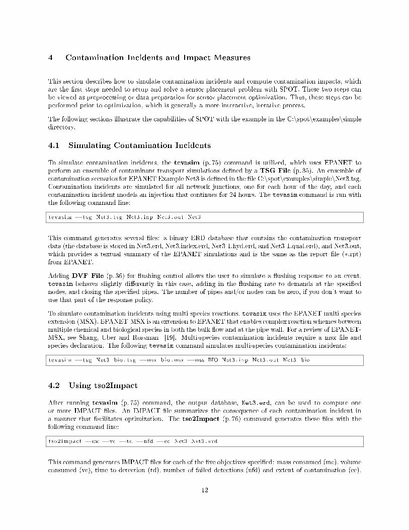
4 Contamination Incidents and Impact Measures

This section describes how to simulate contamination incidents and compute contamination impacts, whichare the �rst steps needed to setup and solve a sensor placement problem with SPOT. These two steps canbe viewed as preprocessing or data preparation for sensor placement optimization. Thus, these steps can beperformed prior to optimization, which is generally a more interactive, iterative process.

The following sections illustrate the capabilities of SPOT with the example in the C:\spot\examples\simpledirectory.

4.1 Simulating Contamination Incidents

To simulate contamination incidents, the tevasim (p. 75) command is utilized, which uses EPANET toperform an ensemble of contaminant transport simulations de�ned by a TSG File (p. 35). An ensemble ofcontamination scenarios for EPANET Example Net3 is de�ned in the �le C:\spot\examples\simple\Net3.tsg.Contamination incidents are simulated for all network junctions, one for each hour of the day, and eachcontamination incident models an injection that continues for 24 hours. The tevasim command is run withthe following command line:

tevasim −−t sg Net3 . t sg Net3 . inp Net3 . out Net3

This command generates several �les: a binary ERD database that contains the contamination transportdata (the database is stored in Net3.erd, Net3.index.erd, Net3-1.hyd.erd, and Net3-1.qual.erd), and Net3.out,which provides a textual summary of the EPANET simulations and is the same as the report �le (∗.rpt)from EPANET.

Adding DVF File (p. 36) for �ushing control allows the user to simulate a �ushing response to an event.tevasim behaves slightly di�erently in this case, adding in the �ushing rate to demands at the speci�ednodes, and closing the speci�ed pipes. The number of pipes and/or nodes can be zero, if you don't want touse that part of the response policy.

To simulate contamination incidents using multi-species reactions, tevasim uses the EPANET multi-speciesextension (MSX). EPANET-MSX is an extension to EPANET that enables complex reaction schemes betweenmultiple chemical and biological species in both the bulk �ow and at the pipe wall. For a review of EPANET-MSX, see Shang, Uber and Rossman [19]. Multi-species contamination incidents require a msx �le andspecies declaration. The following tevasim command simulates multi-species contamination incidents:

tevasim −−t sg Net3_bio . t sg −−msx bio .msx −−mss BIO Net3 . inp Net3 . out Net3_bio

4.2 Using tso2Impact

After running tevasim (p. 75) command, the output database, Net3.erd, can be used to compute oneor more IMPACT �les. An IMPACT �le summarizes the consequence of each contamination incident ina manner that facilitates optimization. The tso2Impact (p. 76) command generates these �les with thefollowing command line:

tso2Impact −−mc −−vc −−td −−nfd −−ec Net3 Net3 . erd

This command generates IMPACT �les for each of the �ve objectives speci�ed: mass consumed (mc), volumeconsumed (vc), time to detection (td), number of failed detections (nfd) and extent of contamination (ec).

12

For each IMPACT �le (e.g. Net3_mc.impact ), a corresponding ID �le is generated to map the sensorplacement ids back to the network junction labels (e.g. Net3_mc.impact.id ).

The impact measures computed by tso2Impact represent the amount of impact that would occur up untilthe point where a contamination incident is detected. This computation assumes that sensors work perfectly(i.e., there are no false positive or false negative errors). However, the sensor behavior can be generalizedin two ways. First, a detection threshold can be speci�ed; contaminants are only detected above a speci�edconcentration limit (the default limit is zero). Second, a response time can be speci�ed, which accountsfor the time needed to verify the presence of contamination (e.g. by �eld investigation) and then informthe public (the default response time is zero). The contamination impact is computed at the time wherethe response has completed (the detection time plus response time), which is called the e�ective response

time. For undetected incidents, the e�ective response time is simply the end of the contaminant transportsimulation. The following illustrates how to specify these options:

tso2Impact −−responseTime 60 −−de te c t i onL imi t 0 . 1 −−mc Net3 Net3 . erd

This computes impacts for a 60 minute response time, with a 0.1 detection threshold. Note that the unitsfor --detectionLimit are the same as for the MASS values that are speci�ed in the TSG �le.

Impacts from multiple ERD �les can be combined to generate a single IMPACT �le using the followingsyntax:

tso2Impact −−de te c t i onL imi t 30000000 −−de te c t i onL imi t 0 .0001 −−mc Net3 Net3_1a . erdNet3_1b . erd

Note that the value of 30000000 corresponds to the detection threshold for the contaminant described inNet3_1a.erd and 0.0001 is the detection threshold for the contaminant described in Net3_1b.erd. Forexample, this can be used to combine simulation results from di�erent types of contaminants, in which theERD �les would have been generated from di�erent TSG �les. Murray et al. [13] use this technique tocombine data from di�erent types of contamination incidents into a single impact metric.

The dvf option speci�es that the demands added due to �ushing be subtracted out prior to calculating theimpact measures. Add this in if the demands creating by simulating �ushing are not �consumed� - i.e., youdon't want the mass included in mass consumed, or other impacts. The time-extent-of-contamination (tec)impact measure integrates the time that each pipe contains contaminated water, rather than just the lengthof pipe that ever contains contaminated water. The result is in units of ft-hrs.

The species option speci�es which species to use to compute impacts. This option is required for multi-speciescontamination incidents created by tevasim. For example:

tso2Impact −−mc −−vc −−td −−nfd −−ec −−s p e c i e s BIO Net3_bio Net3_bio . erd

4.3 Impact Measures

After running tevasim (p. 75) command, the output database, Net3.erd, can be used to compute oneor more IMPACT �les. An IMPACT �le summarizes the consequence of each contamination incident in amanner that facilitates optimization. A variety of objective measures are supported by tso2Impact to re�ectthe di�erent criteria that decision makers could use in CWS design. For most of these criteria, there is adetected and undetected version of the objective. This di�erence concerns how undetected contaminationincidents are modeled.

For example, the default time-to-detection objective, td, uses the time at which the EPANET simulationsare terminated to de�ne the time for incidents that are not detected. The e�ect of this is that undetectedincidents severely penalize sensor network designs. By contrast, the detected time-to-detection, dtd, simply

13

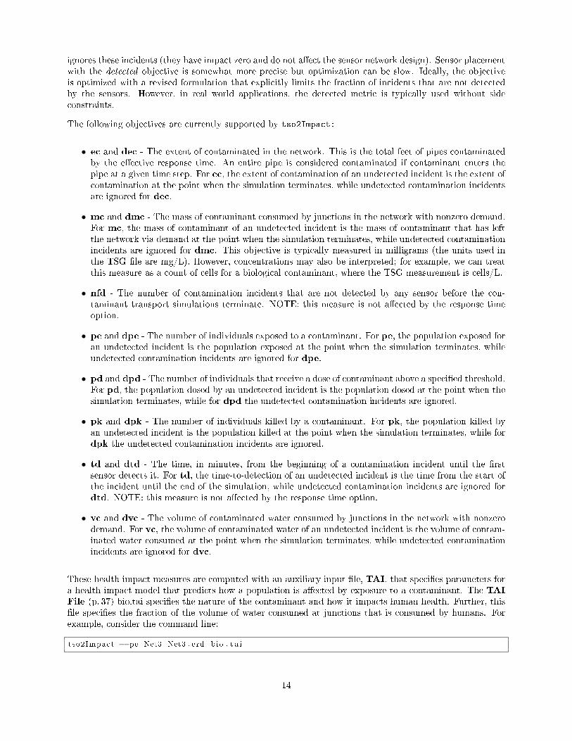
ignores these incidents (they have impact zero and do not a�ect the sensor network design). Sensor placementwith the detected objective is somewhat more precise but optimization can be slow. Ideally, the objectiveis optimized with a revised formulation that explicitly limits the fraction of incidents that are not detectedby the sensors. However, in real world applications, the detected metric is typically used without sideconstraints.

The following objectives are currently supported by tso2Impact:

• ec and dec - The extent of contaminated in the network. This is the total feet of pipes contaminatedby the e�ective response time. An entire pipe is considered contaminated if contaminant enters thepipe at a given time step. For ec, the extent of contamination of an undetected incident is the extent ofcontamination at the point when the simulation terminates, while undetected contamination incidentsare ignored for dec.

• mc and dmc - The mass of contaminant consumed by junctions in the network with nonzero demand.For mc, the mass of contaminant of an undetected incident is the mass of contaminant that has leftthe network via demand at the point when the simulation terminates, while undetected contaminationincidents are ignored for dmc. This objective is typically measured in milligrams (the units used inthe TSG �le are mg/L). However, concentrations may also be interpreted; for example, we can treatthis measure as a count of cells for a biological contaminant, where the TSG measurement is cells/L.

• nfd - The number of contamination incidents that are not detected by any sensor before the con-taminant transport simulations terminate. NOTE: this measure is not a�ected by the response timeoption.

• pe and dpe - The number of individuals exposed to a contaminant. For pe, the population exposed foran undetected incident is the population exposed at the point when the simulation terminates, whileundetected contamination incidents are ignored for dpe.

• pd and dpd - The number of individuals that receive a dose of contaminant above a speci�ed threshold.For pd, the population dosed by an undetected incident is the population dosed at the point when thesimulation terminates, while for dpd the undetected contamination incidents are ignored.

• pk and dpk - The number of individuals killed by a contaminant. For pk, the population killed byan undetected incident is the population killed at the point when the simulation terminates, while fordpk the undetected contamination incidents are ignored.

• td and dtd - The time, in minutes, from the beginning of a contamination incident until the �rstsensor detects it. For td, the time-to-detection of an undetected incident is the time from the start ofthe incident until the end of the simulation, while undetected contamination incidents are ignored fordtd. NOTE: this measure is not a�ected by the response time option.

• vc and dvc - The volume of contaminated water consumed by junctions in the network with nonzerodemand. For vc, the volume of contaminated water of an undetected incident is the volume of contam-inated water consumed at the point when the simulation terminates, while undetected contaminationincidents are ignored for dvc.

These health impact measures are computed with an auxiliary input �le, TAI, that speci�es parameters fora health impact model that predicts how a population is a�ected by exposure to a contaminant. The TAIFile (p. 37) bio.tai speci�es the nature of the contaminant and how it impacts human health. Further, this�le speci�es the fraction of the volume of water consumed at junctions that is consumed by humans. Forexample, consider the command line:

tso2Impact −−pe Net3 Net3 . erd bio . t a i

14

4.4 Advanced Tools for Large Sensor Placements Problems

In some applications, the size of the IMPACT �les is very large, which can lead to optimization models thatcannot be solved on standard 32-bit workstations. SPOT includes several utilities that are not commonly usedto address this challenge: the scenarioAggr (p. 62) executable aggregates similar contamination incidents,and the �lter_impacts (p. 59) script �lters out contamination incidents that have low impacts.

The scenarioAggr (p. 62) executable reads an IMPACT �le, �nds similar incidents, combines them, andwrites out another IMPACT �le. This aggregation technique combines two incidents that impact the samelocations in the same order, allowing for the possibility that one incident continues to impact other locations.For example, two contamination incidents should travel in the same pattern if they di�er only in the nature ofthe contaminant, though one may decay more quickly than the other. Aggregated incidents can be combinedby simply averaging the impacts that they observe and updating the corresponding incident weight.

For example, consider the command:

scenar ioAggr −−numEvents=236 Net3_mc . impact

This creates the �les aggrNet3_mc.impact and aggrNet3_mc.impact.prob; where the Net3_mc.impact

�le has 236 events. The �le aggrNet3_mc.impact is the new IMPACT �le, and the �le aggrNet3_-

mc.impact.prob contains the probabilities of the aggregated incidents.

The �lter_impacts (p. 59) script reads an impact �le, �lters out the low-impact incidents, rescales theimpact values, and writes out another IMPACT �le. The command:

f i l t e r_ impac t s −−percent=5 Net3_mc . impact f i l t e r e d . impact

generates an IMPACT �le that contains the incidents whose impacts (without sensors) are the largest 5%of the incidents in Net3_mc.impact. Similarly, the --num=k option selects the k incidents with the largestimpacts, and the option --threshold=h selects the incidents with the impacts greater than or equal to h.

The filter_impacts command also includes options to rescale the impact values. The --rescale optionrescales impact values with a log-scale and the --round option rescales impact values to rounded log-scalevalues.

15

5 Sensor Placement Solvers

The SPOT sensor placement solvers are launched with the sp (p. 65) command. The sp command reads inone or more IMPACT �les, and computes a sensor placement. Command-line options for sp can specify anyof a set of performance or cost goals as the objective to be optimized, as well as constraints on performanceand cost goals.

The sp command currently interfaces with three di�erent sensor placement optimizers:

• MIP solvers - Several di�erent MIP solvers can be used by the sp command: the commercial CPLEXsolver and the open-source PICO solver. These optimizers use the MIP formulations to �nd globallyoptimal solutions. However, this may be a computationally expensive process (especially for largeproblems), and the size of the MIP formulation can become prohibitively large in some cases.

Two di�erent MIP solvers can be used: the public-domain glpk solver and the commercial solver. PICOis included in distributions of SPOT.

• GRASP heuristic - The GRASP heuristic performs sensor placement optimization without explicitlycreating a MIP formulation. Thus, this solver uses much less memory, and it usually runs very quickly.Although the GRASP heuristic does not guarantee that a globally optimal solution is found, it hasproven e�ective at �nding optimal solutions to a variety of large-scale applications.

Two di�erent implementations of the GRASP solvers can be used: an ATT commercial solver (att_-grasp) and an open-source implementation of this solver (snl_grasp).

• Lagrangian Heuristic - The Lagrangian heuristic uses the structure of the p-median MIP formulation(eSP) to �nd near-optimal solutions while computing a lower bound on the best possible solution.

The following sections provide examples that illustrate the use of the sp command. A description of spcommand line options is available in the Appendix (p. 65).

The sp command has many di�erent options. The following examples show how di�erent sensor place-ment optimization problems can be solved with sp. Note that these examples can be run in theC:\spot\examples\simple directory. The user needs to generate IMPACT �les for these examples withthe following commands:

tevasim −−t sg Net3 . t sg Net3 . inp Net3 . out Net3tso2Impact −−mc −−vc −−td −−nfd −−ec Net3 Net3 . erd

5.1 A Simple Example

The following simple example illustrates the way that SPOT has been most commonly used. In this example,SPOT minimizes the extent of contamination (ec) while limiting the number of sensors (ns) to no more than5. This problem formulation (eSP) can be e�ciently solved with all solvers for modest-size distributionnetworks, and heuristics can e�ectively perform sensor placement on very large networks.

We begin by using the PICO solver to solve this problem, with the following command line:

sp −−path=$bin −−path=$pico −−path=$mod −−network=Net3 −−ob j e c t i v e=ec −−ub=ns , 5 −−s o l v e r=pico

This speci�es that network Net3 is analyzed. The objective is to minimize ec, the extent of contamination,and an upper-bound of 5 is placed on ns, the number of sensors. The solver selected is pico, the PICO MIPsolver.

16

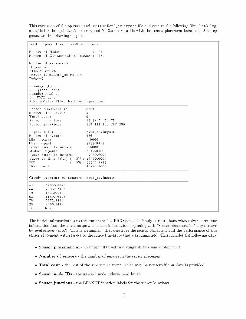
This execution of the sp command uses the Net3_ec.impact �le and creates the following �les: Net3.log,a log�le for the optimization solver, and Net3.sensors, a �le with the sensor placement locations. Also, spgenerates the following output:

read_impact_f i les : Net3_ec . impact

Number o f Nodes : 97Number o f Contamination Impacts : 9480

Number o f s en s o r s=5Object ive=ecS t a t i s t i c=meanImpact f i l e=Net3_ec . impactDelay=0

Running g l p s o l . . .. . . g l p s o l doneRunning PICO . . .. . . PICO done# No weights f i l e : Net3_ec . impact . prob−−−−−−−−−−−−−−−−−−−−−−−−−−−−−−−−−−−−−−−−−−−−−−−−−−−−−−−−−−−−−−−−−−−−−−−−−−−−−−Sensor placement id : 8869Number o f s en s o r s : 5Total co s t : 0Sensor node IDs : 19 28 54 63 75Sensor j unc t i on s : 119 141 193 207 239

Impact F i l e : Net3_ec . impactNumber o f events : 236Min impact : 0 .0000Mean impact : 8499.9419Lower q u a r t i l e impact : 0 .0000Median impact : 6949.0000Upper q u a r t i l e impact : 12530.0000Value at Risk (VaR) ( 5%): 25960.0000TCE ( 5%): 33323.2833Max impact : 42994.8000−−−−−−−−−−−−−−−−−−−−−−−−−−−−−−−−−−−−−−−−−−−−−−−−−−−−−−−−−−−−−−−−−−−−−−−−−−−−−−−−−−−−−−−−−−−−−−−−−−−−−−−−−−−−−−−−−−−−−−−−−−−−−−−−−−−−−−−−−−−−−−−−−−−−−−−−−−−−Greedy orde r ing o f s en s o r s : Net3_ec . impact−−−−−−−−−−−−−−−−−−−−−−−−−−−−−−−−−−−−−−−−−−−−−−−−−−−−−−−−−−−−−−−−−−−−−−−−−−−−−−−1 59035.889054 29087.316519 18650.245363 11492.649675 9972.844528 8499.9419Done with sp

The initial information up to the statement "... PICO done" is simply output about what solver is run andinformation from the solver output. The next information beginning with "Sensor placement id:" is generatedby evalsensor (p. 57). This is a summary that describes the sensor placement and the performance of thissensor placement with respect to the impact measure that was minimized. This includes the following data:

• Sensor placement id - an integer ID used to distinguish this sensor placement

• Number of sensors - the number of sensors in the sensor placement

• Total cost: - the cost of the sensor placement, which may be nonzero if cost data is provided

• Sensor node IDs - the internal node indexes used by sp

• Sensor junctions - the EPANET junction labels for the sensor locations

17

The performance of the sensor placement is summarized for each IMPACT �le used with sp. The impactstatistics included are:

• min - The minimum impact over all contamination events. If we make the assumption that a sensorprotects the node at which it is placed, then this measure will generally be zero.

• mean - The mean (or average) impact over all contamination events.

• lower quartile - 25% of contamination events, weighted by their likelihood, have an impact value lessthan this quartile.

• median - 50% of contamination events, weighted by their likelihood, have an impact value less thanthis quartile.

• upper quartile - 75% of contamination events, weighted by their likelihood, have an impact valueless than this quartile.

• VaR - The value at risk (VaR) uses a user-de�ned percentile. Given 0.0 < β < 1.0, VaR is theminimum value for which 100 ∗ (1− β)% of contamination events have a smaller impact.

• TCE - The tailed-conditioned expectation (TCE) is the mean value of the impacts that are greaterthan or equal to VaR.

• worst - The value of the worst impact.

Finally, a greedy sensor placement is described by evalsensor, which takes the �ve sensor placements andplaces them one-at-a-time, minimizing the mean impact as each sensor is placed. This gives a sense of therelative priorities for these sensors. The evalsensor command can evaluate a sensor placement for a widevariety of di�erent objectives. For example, the command

eva l s en s o r −−nodemap=Net3 . nodemap Net3 . s en s o r s Net3_ec . impact \Net3_mc . impact Net3_nfd . impact

will summarize the solution in the Net3.sensors �le for the ec, mc and nfd impact measures.

The following example shows how to solve this same problem with the GRASP heuristic. This solver �ndsthe same (optimal) solution as the MIP solver, though much more quickly. The command

sp −−path=$bin −−network=Net3 −−ob j e c t i v e=ec −−ub=ns , 5 −−s o l v e r=snl_grasp

generates the following output:

read_impact_f i les : Net3_ec . impactNote : w i tnes s aggregat i on d i s ab l ed f o r grasp



Running i t e r a t e d descent SNL grasp f o r ∗ p e r f e c t ∗ s enso r modelI t e r a t ed descent completed# No weights f i l e : Net3_ec . impact . prob−−−−−−−−−−−−−−−−−−−−−−−−−−−−−−−−−−−−−−−−−−−−−−−−−−−−−−−−−−−−−−−−−−−−−−−−−−−−−−

18

Sensor placement id : 8909Number o f s en s o r s : 5Total co s t : 0Sensor node IDs : 21 33 54 63 75Sensor j unc t i on s : 121 151 193 207 239


Finally, the following example shows how to solve this problem with the Lagrangian heuristic. This solverdoes not �nd as good a solution as the GRASP heuristic. The command

sp −−path=$bin −−network=Net3 −−ob j e c t i v e=ec −−ub=ns , 5 −−s o l v e r=lagrang ian





Se t t i ng up Lagrangian data f i l e s . . .Running UFL s o l v e r . . .. . / . . / . . / bin // u f l Net3_ec . l ag 6 0

# No weights f i l e : Net3_ec . impact . prob−−−−−−−−−−−−−−−−−−−−−−−−−−−−−−−−−−−−−−−−−−−−−−−−−−−−−−−−−−−−−−−−−−−−−−−−−−−−−−Sensor placement id : 8928Number o f s en s o r s : 5Total co s t : 0Sensor node IDs : 19 28 54 63 75Sensor j unc t i on s : 119 141 193 207 239

Impact F i l e : Net3_ec . impactNumber o f events : 236Min impact : 0 .0000Mean impact : 8499.9419Lower q u a r t i l e impact : 0 .0000Median impact : 6949.0000Upper q u a r t i l e impact : 12530.0000

19

Value at Risk (VaR) ( 5%): 25960.0000TCE ( 5%): 33323.2833Max impact : 42994.8000−−−−−−−−−−−−−−−−−−−−−−−−−−−−−−−−−−−−−−−−−−−−−−−−−−−−−−−−−−−−−−−−−−−−−−−−−−−−−−−−−−−−−−−−−−−−−−−−−−−−−−−−−−−−−−−−−−−−−−−−−−−−−−−−−−−−−−−−−−−−−−−−−−−−−−−−−−−−Greedy orde r ing o f s en s o r s : Net3_ec . impact−−−−−−−−−−−−−−−−−−−−−−−−−−−−−−−−−−−−−−−−−−−−−−−−−−−−−−−−−−−−−−−−−−−−−−−−−−−−−−−1 59035.889054 29087.316519 18650.245363 11492.649675 9972.844528 8499.9419Done with sp

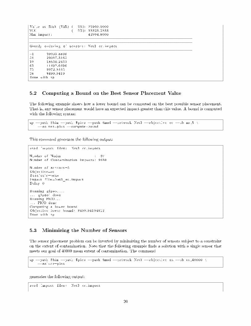
5.2 Computing a Bound on the Best Sensor Placement Value

The following example shows how a lower bound can be computed on the best possible sensor placement.That is, any sensor placement would have an expected impact greater than this value. A bound is computedwith the following syntax:

sp −−path=$bin −−path=$pico −−path=$mod −−network=Net3 −−ob j e c t i v e=ec −−ub=ns , 5 \−−s o l v e r=pico −−compute−bound

This command generates the following output:




Running g l p s o l . . .. . . g l p s o l doneRunning PICO . . .. . . PICO doneComputing a lower boundObject ive lower bound : 8499.94194912Done with sp

5.3 Minimizing the Number of Sensors

The sensor placement problem can be inverted by minimizing the number of sensors subject to a constrainton the extent of contamination. Note that the following example �nds a solution with a single sensor thatmeets our goal of 40000 mean extent of contamination. The command

sp −−path=$bin −−path=$pico −−path=$mod −−network=Net3 −−ob j e c t i v e=ns −−ub=ec ,40000 \−−s o l v e r=pico



20


WARNING: Locat ion aggregat i on does not work with s i d e c on s t r a i n t sWARNING: Turning o f f l o c a t i o n aggregat ionNumber o f s en s o r s=nsObject ive=nsS t a t i s t i c=meanImpact f i l e=Net3_ns . impactDelay=0

Running g l p s o l . . .. . . g l p s o l doneRunning PICO . . .. . . PICO done# No weights f i l e : Net3_ec . impact . prob−−−−−−−−−−−−−−−−−−−−−−−−−−−−−−−−−−−−−−−−−−−−−−−−−−−−−−−−−−−−−−−−−−−−−−−−−−−−−−Sensor placement id : 9196Number o f s en s o r s : 1Total co s t : 0Sensor node IDs : 37Sensor j unc t i on s : 161

Impact F i l e : Net3_ec . impactNumber o f events : 236Min impact : 0 .0000Mean impact : 27097.7191Lower q u a r t i l e impact : 3940.0000Median impact : 22450.0000Upper q u a r t i l e impact : 38855.0000Value at Risk (VaR) ( 5%): 71377.8000TCE ( 5%): 81046.0667Max impact : 103746.0000−−−−−−−−−−−−−−−−−−−−−−−−−−−−−−−−−−−−−−−−−−−−−−−−−−−−−−−−−−−−−−−−−−−−−−−−−−−−−−−−−−−−−−−−−−−−−−−−−−−−−−−−−−−−−−−−−−−−−−−−−−−−−−−−−−−−−−−−−−−−−−−−−−−−−−−−−−−−Greedy orde r ing o f s en s o r s : Net3_ec . impact−−−−−−−−−−−−−−−−−−−−−−−−−−−−−−−−−−−−−−−−−−−−−−−−−−−−−−−−−−−−−−−−−−−−−−−−−−−−−−−1 59035.889037 27097.7191Done with sp

5.4 Fixing Sensor Placement Locations

Properties of the sensor locations can be speci�ed with the --sensor-locations option. This optionsspeci�es a Placement Locations File (p. 42) that can control whether sensor locations are feasible orinfeasible, and �xed or un�xed. For example, suppose the �le locations contains

i n f e a s i b l e 193 119 141 207 239f i x ed 161

The following example shows how these restrictions impact the solution. Compared to the �rst exampleabove, we have a less-optimal solution, since the sensor locations above cannot be used and junction 161

must be included. The command

sp −−path=$bin −−path=$pico −−path=$mod −−network=Net3 −−ob j e c t i v e=ec −−ub=ns , 5 \−−s o l v e r=pico −−sensor−l o c a t i o n s=l o c a t i o n s



21



Running g l p s o l . . .. . . g l p s o l doneRunning PICO . . .. . . PICO done# No weights f i l e : Net3_ec . impact . prob−−−−−−−−−−−−−−−−−−−−−−−−−−−−−−−−−−−−−−−−−−−−−−−−−−−−−−−−−−−−−−−−−−−−−−−−−−−−−−Sensor placement id : 9273Number o f s en s o r s : 5Total co s t : 0Sensor node IDs : 17 33 37 50 66Sensor j unc t i on s : 115 151 161 185 211


5.5 Robust Optimization of Sensor Locations

The following example demonstrates the optimization of sensor placements using the TCE measure. TCE isthe mean value of the worst incidents in the ensemble being evaluated. Given a con�dence level 1− β, TCEis the expectation of the worst impacts with probability β. Compared with our �rst example, this �nds abetter solution in terms of TCE, although the mean performance is slightly worse.

The command

sp −−path=$bin −−network=Net3 −−ob j e c t i v e=ec_tce −−ub=ns , 5 −−s o l v e r=snl_grasp




Number o f s en s o r s=5

22

Object ive=ecS t a t i s t i c=tceImpact f i l e=Net3_ec . impactDelay=0

Running i t e r a t e d descent SNL grasp f o r ∗ p e r f e c t ∗ s enso r modelI t e r a t ed descent completed# No weights f i l e : Net3_ec . impact . prob−−−−−−−−−−−−−−−−−−−−−−−−−−−−−−−−−−−−−−−−−−−−−−−−−−−−−−−−−−−−−−−−−−−−−−−−−−−−−−Sensor placement id : 9289Number o f s en s o r s : 5Total co s t : 0Sensor node IDs : 17 19 24 65 88Sensor j unc t i on s : 115 119 127 209 267

Impact F i l e : Net3_ec . impactNumber o f events : 236Min impact : 0 .0000Mean impact : 10287.0856Lower q u a r t i l e impact : 1650.0000Median impact : 10400.0000Upper q u a r t i l e impact : 16930.0000Value at Risk (VaR) ( 5%): 24199.0000TCE ( 5%): 26376.2167Max impact : 28564.8000−−−−−−−−−−−−−−−−−−−−−−−−−−−−−−−−−−−−−−−−−−−−−−−−−−−−−−−−−−−−−−−−−−−−−−−−−−−−−−−−−−−−−−−−−−−−−−−−−−−−−−−−−−−−−−−−−−−−−−−−−−−−−−−−−−−−−−−−−−−−−−−−−−−−−−−−−−−−Greedy orde r ing o f s en s o r s : Net3_ec . impact−−−−−−−−−−−−−−−−−−−−−−−−−−−−−−−−−−−−−−−−−−−−−−−−−−−−−−−−−−−−−−−−−−−−−−−−−−−−−−−1 59035.889088 30705.948719 19271.898365 12589.056817 11151.390724 10287.0856Done with sp

Note that the greedy ordering of sensors is less useful in this case. Although we optimized to minimize TCE,the greedy ordering uses the mean value to select each sensor location.

5.6 Multi-Criteria Analysis

The sp command supports multi-objective analysis through an iterative process. SPOT does not have ageneral "pareto search" optimizer. Instead, users can specify constraints with sp that ensure that previouslyoptimized objectives are "close" to their previous values. In this way, the user can explicitly search fortrade-o�s between one-or-more performance objectives.

The examples above consider the extent-of-contamination objective. The sensor placements generated abovecan be assessed as to how they minimize other objectives like the expected mass of contaminant consumedusing evalsensor. Consider the solution generated by the previous example (which minimized ec_tce),which was copied into the �le Net3_ec.sensors.

The command

eva l s en s o r −−nodemap=Net3 . nodemap Net3_ec . s en s o r s Net3_mc . impact


# No weights f i l e : Net3_mc . impact . prob−−−−−−−−−−−−−−−−−−−−−−−−−−−−−−−−−−−−−−−−−−−−−−−−−−−−−−−−−−−−−−−−−−−−−−−−−−−−−−Sensor placement id : 9304

23

Number o f s en s o r s : 5Total co s t : 0Sensor node IDs : 17 19 24 65 88Sensor j unc t i on s : 115 119 127 209 267

Impact F i l e : Net3_mc . impactNumber o f events : 236Min impact : 0 .0000Mean impact : 70907.8333Lower q u a r t i l e impact : 503.9170Median impact : 83150.7000Upper q u a r t i l e impact : 143999.0000Value at Risk (VaR) ( 5%): 144329.0000TCE ( 5%): 144555.3333Max impact : 144732.0000−−−−−−−−−−−−−−−−−−−−−−−−−−−−−−−−−−−−−−−−−−−−−−−−−−−−−−−−−−−−−−−−−−−−−−−−−−−−−−−−−−−−−−−−−−−−−−−−−−−−−−−−−−−−−−−−−−−−−−−−−−−−−−−−−−−−−−−−−−−−−−−−−−−−−−−−−−−−Greedy orde r ing o f s en s o r s : Net3_mc . impact−−−−−−−−−−−−−−−−−−−−−−−−−−−−−−−−−−−−−−−−−−−−−−−−−−−−−−−−−−−−−−−−−−−−−−−−−−−−−−−1 137028.526365 71611.965888 71269.077524 71055.007617 70965.273819 70907.8333

The mean mass consumed is 70907, which is far from the optimal value of 21782 (which we computed sepa-rately). The robust optimization example in the previous section is revisited here; "extent of contamination- tce" is still the primary objective, but now a "side constraint" is imposed that precludes any solution thatadmits an average mass consumed of worse than 30,000 units. The command

#!/bin / sh

bin=`pwd ` / . . / . . / . . / binmod=`pwd ` / . . / . . / . . / e t c /modpico=`pwd ` / . . / . . / . . / . . / acro−pico /binpythonpath=`pwd ` / . . / . . / . . / python/binexport PATH=$bin : $pythonpath : $p ico :$PATH

i f [ ! −e Net3 . erd ] ; then# @prelim :tevasim −−t sg Net3 . t sg Net3 . inp Net3 . out Net3tso2Impact −−mc −−vc −−td −−nfd −−ec Net3 Net3 . erd# @: pre l ime l s ecp data/Net3 . erd .cp data/Net3 ∗ . erd .i f [ ! −e Net3_mc . impact ] ; thentso2Impact −−mc −−vc −−td −−nfd −−ec Net3 Net3 . erdf if i

# @sp :sp −−path=$bin −−network=Net3 −−ob j e c t i v e=ec_tce −−ub=mc_mean,30000 −−ub=ns , 5 \

−−s o l v e r=snl_grasp# @: sp


read_impact_f i les : Net3_ec . impactread_impact_f i les : Net3_mc . impactNote : w i tnes s aggregat i on d i s ab l ed f o r grasp

Number o f Nodes : 97

24

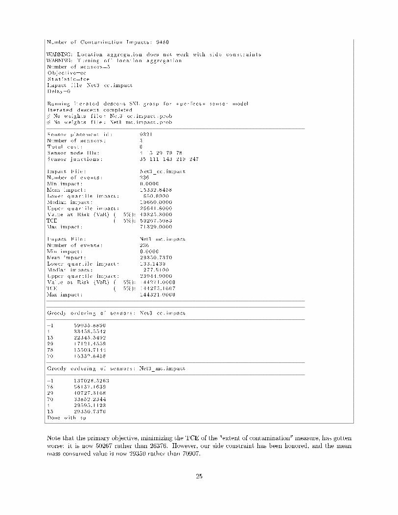
Number o f Contamination Impacts : 9480

WARNING: Locat ion aggregat i on does not work with s i d e c on s t r a i n t sWARNING: Turning o f f l o c a t i o n aggregat ionNumber o f s en s o r s=5Object ive=ecS t a t i s t i c=tceImpact f i l e=Net3_ec . impactDelay=0

Running i t e r a t e d descent SNL grasp f o r ∗ p e r f e c t ∗ s enso r modelI t e r a t ed descent completed# No weights f i l e : Net3_ec . impact . prob# No weights f i l e : Net3_mc . impact . prob−−−−−−−−−−−−−−−−−−−−−−−−−−−−−−−−−−−−−−−−−−−−−−−−−−−−−−−−−−−−−−−−−−−−−−−−−−−−−−Sensor placement id : 9321Number o f s en s o r s : 5Total co s t : 0Sensor node IDs : 4 15 29 70 78Sensor j unc t i on s : 35 111 143 219 247

Impact F i l e : Net3_ec . impactNumber o f events : 236Min impact : 0 .0000Mean impact : 15332.8458Lower q u a r t i l e impact : 1650.0000Median impact : 10660.0000Upper q u a r t i l e impact : 26641.8000Value at Risk (VaR) ( 5%): 40825.8000TCE ( 5%): 50267.5083Max impact : 71329.0000

Impact F i l e : Net3_mc . impactNumber o f events : 236Min impact : 0 .0000Mean impact : 29350.7370Lower q u a r t i l e impact : 133.1430Median impact : 1277.5100Upper q u a r t i l e impact : 23944.9000Value at Risk (VaR) ( 5%): 144271.0000TCE ( 5%): 144275.1667Max impact : 144321.0000−−−−−−−−−−−−−−−−−−−−−−−−−−−−−−−−−−−−−−−−−−−−−−−−−−−−−−−−−−−−−−−−−−−−−−−−−−−−−−−−−−−−−−−−−−−−−−−−−−−−−−−−−−−−−−−−−−−−−−−−−−−−−−−−−−−−−−−−−−−−−−−−−−−−−−−−−−−−Greedy orde r ing o f s en s o r s : Net3_ec . impact−−−−−−−−−−−−−−−−−−−−−−−−−−−−−−−−−−−−−−−−−−−−−−−−−−−−−−−−−−−−−−−−−−−−−−−−−−−−−−−1 59035.88904 33458.554215 22345.549229 17121.455978 15503.714470 15332.8458−−−−−−−−−−−−−−−−−−−−−−−−−−−−−−−−−−−−−−−−−−−−−−−−−−−−−−−−−−−−−−−−−−−−−−−−−−−−−−Greedy orde r ing o f s en s o r s : Net3_mc . impact−−−−−−−−−−−−−−−−−−−−−−−−−−−−−−−−−−−−−−−−−−−−−−−−−−−−−−−−−−−−−−−−−−−−−−−−−−−−−−−1 137028.526378 58137.163929 40727.316870 33852.23444 29595.112315 29350.7370Done with sp

Note that the primary objective, minimizing the TCE of the "extent of contamination" measure, has gottenworse: it is now 50267 rather than 26376. However, our side constraint has been honored, and the meanmass consumed value is now 29350 rather than 70907.

25

5.7 Sensor Placements without Penalties

A fundamental issue for sensor placement is how to handle the fact that a limited budget of sensors will not beable to cover all possible incidents. SPOT addresses this issue by providing impact measures that integratean impact 'penalty' for incidents that are not detected by a CWS design. Thus, in the previous examplesthere was an implicit trade-o� between impact reduction and reduction in the number of contaminationincidents that are detected.

SPOT also includes impact measures that do not contain these penalties, which allows a user to more directlyassess the performance of a CWS design in the context where detections have occurred. For example,the time-to-detection measure (td) includes a penalty for undetected incidents, but the detected-time-to-detection measure (dtd) has no penalty (or, more precisely, a zero penalty).

For example, consider the simple example above, which minimizes the extent of contamination. Theevalsensors command is applied to the �nal solution to evaluate the ec, dec and nfd impact measures:

eva l s en s o r −−nodemap=Net3 . nodemap Net3_orig . s en s o r s Net3_ec . impact Net3_dec . impact \Net3_nfd . impact

This generates the following output:

# No weights f i l e : Net3_ec . impact . prob# No weights f i l e : Net3_dec . impact . prob# No weights f i l e : Net3_nfd . impact . prob−−−−−−−−−−−−−−−−−−−−−−−−−−−−−−−−−−−−−−−−−−−−−−−−−−−−−−−−−−−−−−−−−−−−−−−−−−−−−−Sensor placement id : 9360Number o f s en s o r s : 5Total co s t : 0Sensor node IDs : 19 28 54 63 75Sensor j unc t i on s : 119 141 193 207 239

Impact F i l e : Net3_ec . impactNumber o f events : 236Min impact : 0 .0000Mean impact : 8499.9419Lower q u a r t i l e impact : 0 .0000Median impact : 6949.0000Upper q u a r t i l e impact : 12530.0000Value at Risk (VaR) ( 5%): 25960.0000TCE ( 5%): 33323.2833Max impact : 42994.8000

Impact F i l e : Net3_dec . impactNumber o f events : 236Min impact : 0 .0000Mean impact : 8184.5182Lower q u a r t i l e impact : 0 .0000Median impact : 6949.0000Upper q u a r t i l e impact : 12530.0000Value at Risk (VaR) ( 5%): 25960.0000TCE ( 5%): 33323.2833Max impact : 42994.8000

Impact F i l e : Net3_nfd . impactNumber o f events : 236Min impact : 0 .0000Mean impact : 0 .2500Lower q u a r t i l e impact : 0 .0000Median impact : 0 .0000Upper q u a r t i l e impact : 0 .0000Value at Risk (VaR) ( 5%): 1 .0000TCE ( 5%): 1 .0000Max impact : 1 .0000

26

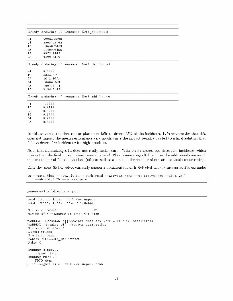
−−−−−−−−−−−−−−−−−−−−−−−−−−−−−−−−−−−−−−−−−−−−−−−−−−−−−−−−−−−−−−−−−−−−−−−−−−−−−−−−−−−−−−−−−−−−−−−−−−−−−−−−−−−−−−−−−−−−−−−−−−−−−−−−−−−−−−−−−−−−−−−−−−−−−−−−−−−−Greedy orde r ing o f s en s o r s : Net3_ec . impact−−−−−−−−−−−−−−−−−−−−−−−−−−−−−−−−−−−−−−−−−−−−−−−−−−−−−−−−−−−−−−−−−−−−−−−−−−−−−−−1 59035.889054 29087.316519 18650.245363 11492.649675 9972.844528 8499.9419−−−−−−−−−−−−−−−−−−−−−−−−−−−−−−−−−−−−−−−−−−−−−−−−−−−−−−−−−−−−−−−−−−−−−−−−−−−−−−Greedy orde r ing o f s en s o r s : Net3_dec . impact−−−−−−−−−−−−−−−−−−−−−−−−−−−−−−−−−−−−−−−−−−−−−−−−−−−−−−−−−−−−−−−−−−−−−−−−−−−−−−−1 0 .000019 4845.777128 3613.467854 10806.363163 7097.611475 8184.5182−−−−−−−−−−−−−−−−−−−−−−−−−−−−−−−−−−−−−−−−−−−−−−−−−−−−−−−−−−−−−−−−−−−−−−−−−−−−−−Greedy orde r ing o f s en s o r s : Net3_nfd . impact−−−−−−−−−−−−−−−−−−−−−−−−−−−−−−−−−−−−−−−−−−−−−−−−−−−−−−−−−−−−−−−−−−−−−−−−−−−−−−−1 1 .000075 0 .271228 0 .250019 0 .250054 0 .250063 0 .2500

In this example, the �nal sensor placement fails to detect 25% of the incidents. It is noteworthy that thisdoes not impact the mean performance very much, since the impact penalty has led to a �nal solution thatfails to detect few incidents with high penalties.

Note that minimizing dtd does not really make sense. With zero sensors, you detect no incidents, whichmeans that the �nal impact measurement is zero! Thus, minimizing dtd requires the additional constrainton the number of failed detections (nfd) as well as a limit on the number of sensors (or total sensor costs).

Only the 'pico' SPOT solver currently supports optimization with 'detected' impact measures. For example:

sp −−path=$bin −−path=$pico −−path=$mod −−network=Net3 −−ob j e c t i v e=dec −−ub=ns , 5 \−−ub=nfd , 0 . 2 5 −−s o l v e r=pico


read_impact_f i les : Net3_dec . impactread_impact_f i les : Net3_nfd . impact


WARNING: Locat ion aggregat i on does not work with s i d e c on s t r a i n t sWARNING: Turning o f f l o c a t i o n aggregat ionNumber o f s en s o r s=5Object ive=decS t a t i s t i c=meanImpact f i l e=Net3_dec . impactDelay=0

Running g l p s o l . . .. . . g l p s o l doneRunning PICO . . .. . . PICO done# No weights f i l e : Net3_dec . impact . prob

27

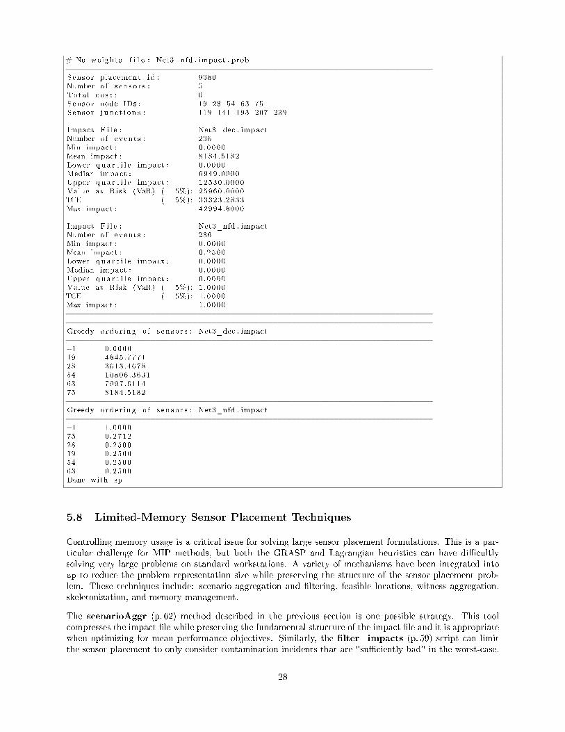
# No weights f i l e : Net3_nfd . impact . prob−−−−−−−−−−−−−−−−−−−−−−−−−−−−−−−−−−−−−−−−−−−−−−−−−−−−−−−−−−−−−−−−−−−−−−−−−−−−−−Sensor placement id : 9380Number o f s en s o r s : 5Total co s t : 0Sensor node IDs : 19 28 54 63 75Sensor j unc t i on s : 119 141 193 207 239

Impact F i l e : Net3_dec . impactNumber o f events : 236Min impact : 0 .0000Mean impact : 8184.5182Lower q u a r t i l e impact : 0 .0000Median impact : 6949.0000Upper q u a r t i l e impact : 12530.0000Value at Risk (VaR) ( 5%): 25960.0000TCE ( 5%): 33323.2833Max impact : 42994.8000

Impact F i l e : Net3_nfd . impactNumber o f events : 236Min impact : 0 .0000Mean impact : 0 .2500Lower q u a r t i l e impact : 0 .0000Median impact : 0 .0000Upper q u a r t i l e impact : 0 .0000Value at Risk (VaR) ( 5%): 1 .0000TCE ( 5%): 1 .0000Max impact : 1 .0000−−−−−−−−−−−−−−−−−−−−−−−−−−−−−−−−−−−−−−−−−−−−−−−−−−−−−−−−−−−−−−−−−−−−−−−−−−−−−−−−−−−−−−−−−−−−−−−−−−−−−−−−−−−−−−−−−−−−−−−−−−−−−−−−−−−−−−−−−−−−−−−−−−−−−−−−−−−−Greedy orde r ing o f s en s o r s : Net3_dec . impact−−−−−−−−−−−−−−−−−−−−−−−−−−−−−−−−−−−−−−−−−−−−−−−−−−−−−−−−−−−−−−−−−−−−−−−−−−−−−−−1 0 .000019 4845.777128 3613.467854 10806.363163 7097.611475 8184.5182−−−−−−−−−−−−−−−−−−−−−−−−−−−−−−−−−−−−−−−−−−−−−−−−−−−−−−−−−−−−−−−−−−−−−−−−−−−−−−Greedy orde r ing o f s en s o r s : Net3_nfd . impact−−−−−−−−−−−−−−−−−−−−−−−−−−−−−−−−−−−−−−−−−−−−−−−−−−−−−−−−−−−−−−−−−−−−−−−−−−−−−−−1 1 .000075 0 .271228 0 .250019 0 .250054 0 .250063 0 .2500Done with sp

5.8 Limited-Memory Sensor Placement Techniques

Controlling memory usage is a critical issue for solving large sensor placement formulations. This is a par-ticular challenge for MIP methods, but both the GRASP and Lagrangian heuristics can have di�cultlysolving very large problems on standard workstations. A variety of mechanisms have been integrated intosp to reduce the problem representation size while preserving the structure of the sensor placement prob-lem. These techniques include: scenario aggregation and �ltering, feasible locations, witness aggregation,skeletonization, and memory management.

The scenarioAggr (p. 62) method described in the previous section is one possible strategy. This toolcompresses the impact �le while preserving the fundamental structure of the impact �le and it is appropriatewhen optimizing for mean performance objectives. Similarly, the �lter_impacts (p. 59) script can limitthe sensor placement to only consider contamination incidents that are "su�ciently bad" in the worst-case.

28

Another strategy is to limit the number of sensor placements, using the --sensor-locations option de-scribed above. Eliminating feasible locations reduces the problem representation used by the sp solvers.

The witness aggregation technique can be used to limit the size of the sensor placement formulation. Thisterm refers to the variables in the MIP formulation that "witness" a contamination event. By default,variables that witness contamination events with the same impact are aggregated, and this typically reducesthe MIP constraint matrix by a signi�cant amount. Further reductions can be performed with more aggressiveaggregations.

To illustrate the use of witness aggregation, we generated impact �les with the C:\spot\etc\tsg\hourly.tsgTSG �le. The following table illustrates the use of the two witness aggregation options when optimizingthe mean extent of contamination: --aggregation-percent and --aggregation-ratio (used with the--distinguish-detection option, which helps this aggregation option). The second line of data in thistable is the default aggregation, which has about half as many non-zero values in the MIP constraint matrix.Both the percent and ratio aggregation strategies e�ectively reduce the problem size while �nding near-optimal solutions.

Aggr Type Aggr Value Binary Vars MIP Nonzeros Solution ValueNone NA 97 220736 8525Percent 0.0 97 119607 8525Percent 0.125 97 49576 9513Ratio 0.125 97 12437 10991

Another option to reduce the memory requirement for sensor placement is to reduce the size of the networkmodel through skeletonization. Skeletonization groups neighboring nodes based on the topology of thenetwork and pipe attributes. The TEVA-SPOT Skeleton code, spotSkeleton (p. 73), provides techniquesfor branch trimming, series pipe merging, and parallel pipe merging. Skeletonization eliminates pipes andjunctions that have little impact on the overall hydraulics of the system. This e�ectively contracts a connectedpiece of the network into a single node, called a supernode. Skeletonized networks can be used to de�negeographic proximity in a two-tiered sensor placement approach for large network models. Details on thetwo-tiered sensor placement approach can be found in Section 5.9 (p. 29).

Additionally, the GRASP heuristic has several options for controlling how memory is managed. The--grasp-representation option can be used to control how the local search steps are performed. Bydefault, a dense matrix is precomputed to perform local search steps quickly, but a sparse matrix can beused to perform local search with less memory. Also, the GRASP heuristic can be con�gured to use thelocal disk to store this matrix. It should be noted that the Lagrangian heuristic requires less memory thanthe GRASP heuristic, and thus similar techniques have not been developed for it.

5.9 Two-tiered Sensor Placement Approach

The two-tiered sensor placement approach uses geographic aggregation on the large impact �les to selectcandidate locations for secondary optimization. While the approach uses detailed hydraulic calculations, itavoids solving sensor placement using the large impact �le directly, a process that can exceed the memoryavailable on a personal computer. Geographic aggregation combines witness locations over all scenariosbased on their geographic proximity. To maintain hydraulic equivalence as much as possible, skeletonizationis used to de�ne geographic proximity. This process is similar to witness aggregation, where witness locationsfor a single scenario are combined based upon their witness quality. In both cases, the number of possiblesensor locations is reduced.

Geographic aggregation reduces the impact �le by grouping nodes that are co-located in the skeletonizationprocess. In essence, this reduces the impact �le to include only skeletonized nodes (i.e. supernodes) de�nedin the skeletonized network. From the skeletonized viewpoint, the contaminant hits a supernode when it�rst crosses the curve de�ning the supernode. Depending upon the direction the contaminant approaches, it

29

will hit the real nodes inside the supernodes in di�erent orders. With geographic aggregation, the minimum,maximum, mean, or median could be used to group the time and impact for the real nodes in each supernode.For a sensor on a single real node in the supernode, the maximum statistic is pessimistic for incidents thatthe node detects. Similarly, using the minimum is always optimistic. For example, consider one supernodethat represents four nodes in the original network. The impact values for those nodes are 100, 200, 250, and300. After geographic aggregation, the impact value is 100 using the minimum, 300 using the maximum,212.5 using the mean, and 225 using the median. The time associated with each of these impacts is groupedthe same way. The new time and impact pair is the aggregated representation of the impact �le for thatnode. For this supernode, four lines of the impact �le are reduced to one. This aggregation is performedfor each scenario and each supernode. While this greatly reduces the size of the impact �le, the number ofscenarios remains the same. This method is not in�uenced by the modi�ed hydraulics of the skeletonizednetwork; rather, the original impact �le is modi�ed to re�ect geographic aggregation from the skeletonizednetwork.

In the �rst-tier (Tier 1), sensor placement �lters candidate sensor locations based on a geographic aggrega-tion of the impact �le. Heuristically, sensor placement in this course search identi�es supernodes that arepromising regions for sensors. Only real nodes within these selected supernodes are considered candidatesensor locations. All other locations from the impact �le generated from the original, most-re�ned networkmodel are removed. The second-tier (Tier 2) sensor placement uses this re�ned impact �le to place sensorsin the original network. Since sensor placement in each tier runs on a smaller impact �le than a directplacement on the original network, the two-tiered approach reduces the maximum memory requirement.

The two-tiered sensor placement approach can be run using sp-2tier (p. 70). The method calls spotSkele-ton (p. 73) to de�ne geographic proximity from skeletonized networks. The two-tiered method has beenshown to maintain solution quality while greatly reducing the memory footprint need for sensor placement.For additional details, see Klise, Phillips, and Janke [10].

The sp-2tier executable is run with the following command line:

sp−2 t i e r −−path=$bin −−network=Net3 −−ob j e c t i v e=mc −−s k e l e t on=8 −−s t a t=min\−−ub1=ns , 5 −−ub2=ns , 5 −−s o l v e r 1=snl_grasp −−s o l v e r 2=snl_grasp

This command generates aggregated and re�ned impact �les, along with output �les from sp based on Tier1 and Tier 2 sensor placement.

5.10 Evaluating a Sensor Placement

The evalsensor (p. 57) executable takes sensor placements in a Sensor Placement File (p. 39) and eval-uates them using data from an Impact File (p. 40) (or a list of impact �les). This executable measures theperformance of each sensor placement with respect to the set of possible contamination locations. This anal-ysis assumes that probabilities have been assigned to these contamination locations, and if no probabilitiesare given then uniform probabilities are used by evalsensor.

The following example illustrates the use of evalsensor after running the �rst sensor placement optimizationexample. The command

eva l s en s o r −−nodemap=Net3 . nodemap Net3_orig . s en s o r s Net3_ec . impact Net3_mc . impact


# No weights f i l e : Net3_ec . impact . prob# No weights f i l e : Net3_mc . impact . prob−−−−−−−−−−−−−−−−−−−−−−−−−−−−−−−−−−−−−−−−−−−−−−−−−−−−−−−−−−−−−−−−−−−−−−−−−−−−−−Sensor placement id : 9404Number o f s en s o r s : 5

30

Total co s t : 0Sensor node IDs : 19 28 54 63 75Sensor j unc t i on s : 119 141 193 207 239

Impact F i l e : Net3_ec . impactNumber o f events : 236Min impact : 0 .0000Mean impact : 8499.9419Lower q u a r t i l e impact : 0 .0000Median impact : 6949.0000Upper q u a r t i l e impact : 12530.0000Value at Risk (VaR) ( 5%): 25960.0000TCE ( 5%): 33323.2833Max impact : 42994.8000

Impact F i l e : Net3_mc . impactNumber o f events : 236Min impact : 0 .0000Mean impact : 43649.6779Lower q u a r t i l e impact : 220.0020Median impact : 1903.6700Upper q u a r t i l e impact : 105363.0000Value at Risk (VaR) ( 5%): 144271.0000TCE ( 5%): 144327.6667Max impact : 144477.0000−−−−−−−−−−−−−−−−−−−−−−−−−−−−−−−−−−−−−−−−−−−−−−−−−−−−−−−−−−−−−−−−−−−−−−−−−−−−−−−−−−−−−−−−−−−−−−−−−−−−−−−−−−−−−−−−−−−−−−−−−−−−−−−−−−−−−−−−−−−−−−−−−−−−−−−−−−−−Greedy orde r ing o f s en s o r s : Net3_ec . impact−−−−−−−−−−−−−−−−−−−−−−−−−−−−−−−−−−−−−−−−−−−−−−−−−−−−−−−−−−−−−−−−−−−−−−−−−−−−−−−1 59035.889054 29087.316519 18650.245363 11492.649675 9972.844528 8499.9419−−−−−−−−−−−−−−−−−−−−−−−−−−−−−−−−−−−−−−−−−−−−−−−−−−−−−−−−−−−−−−−−−−−−−−−−−−−−−−Greedy orde r ing o f s en s o r s : Net3_mc . impact−−−−−−−−−−−−−−−−−−−−−−−−−−−−−−−−−−−−−−−−−−−−−−−−−−−−−−−−−−−−−−−−−−−−−−−−−−−−−−−1 137028.526375 59420.206928 44491.590863 43867.975254 43672.700919 43649.6779

The evalsensors command can also evaluate a sensor placement in the case where sensors can fail, and thereis some small number of di�erent classes of sensors (grouped by false negative probability). This informationis de�ned by a Sensor Class File (p. 43) and a Junction Class File (p. 43). Consider the sensor class orsc �le, Net3.imperfectsc, which de�nes di�erent categories of sensor failures:

1 0 .252 0 .503 0 .754 1 .0

Sensors of class "1" give false negative readings 25% of the time, sensors of class "2" give them 50% of thetime, etc.

Once failure classes have been de�ned, the junctions of the network are assigned to classes. This is donewith a junction class or jc �le, like Net3.imperfectjc (here we show just the beginning of this �le):

1 12 1

31

3 14 15 16 17 18 19 110 1

Given the junction classes, we can run evalsensor to determine the expected impact of a sensor placement,given that sensors may fail. Again, using the solution from the original example:

eva l s en s o r −−nodemap=Net3 . nodemap −−sc−p r o b a b i l i t i e s=Net3 . impe r f e c t s c \−−s c s=Net3 . impe r f e c t j c Net3_orig . s en s o r s Net3_ec . impact


AA# No weights f i l e : Net3_ec . impact . prob−−−−−−−−−−−−−−−−−−−−−−−−−−−−−−−−−−−−−−−−−−−−−−−−−−−−−−−−−−−−−−−−−−−−−−−−−−−−−−Sensor placement id : 9425Number o f s en s o r s : 5Total co s t : 0Sensor node IDs : 19 28 54 63 75Sensor j unc t i on s : 119 141 193 207 239

Impact F i l e : Net3_ec . impactNumber o f events : 236Min impact : 0 .0000Mean impact : 17193.3515Lower q u a r t i l e impact : 3940.0000Median impact : 15307.2500Upper q u a r t i l e impact : 26537.2156Value at Risk (VaR) ( 5%): 47637.7773TCE ( 5%): 54977.0644Max impact : 75509.9043−−−−−−−−−−−−−−−−−−−−−−−−−−−−−−−−−−−−−−−−−−−−−−−−−−−−−−−−−−−−−−−−−−−−−−−−−−−−−−−−−−−−−−−−−−−−−−−−−−−−−−−−−−−−−−−−−−−−−−−−−−−−−−−−−−−−−−−−−−−−−−−−−−−−−−−−−−−−Greedy orde r ing o f s en s o r s : Net3_ec . impact−−−−−−−−−−−−−−−−−−−−−−−−−−−−−−−−−−−−−−−−−−−−−−−−−−−−−−−−−−−−−−−−−−−−−−−−−−−−−−−1 59035.889054 36574.459663 25675.975428 21230.246375 18841.648819 17193.3515

Note that the mean impact of this "extent of contamination" changes dramatically if sensors are allowed tofail. The original solution, 8499 pipe feet, was misleading if sensors fail according to the probabilities wehave assigned. With sensor failures, the expected impact is 17193 pipe feet -- more than twice the "perfectsensor" impact.

5.11 Sensor Placement with Imperfect Sensors

The GRASP heuristics in SPOT can optimize sensor placements that take into account sensor failures. Forexample, we can perform sensor placement optimization with imperfect sensors using the Net3.imperfectscand Net3.imperfectjc �les de�ned in the previous section. The command

sp −−path=$bin −−network=Net3 −−ob j e c t i v e=ec −−ub=ns , 5 −−imper fect− s c f i l e=Net3 . impe r f e c t s c \−−imper fect− j c f i l e=Net3 . impe r f e c t j c −−s o l v e r=snl_grasp

32





Running i t e r a t e d descent grasp f o r ∗ imper f e c t ∗ s enso r modelI t e r a t ed descent completed# No weights f i l e : Net3_ec . impact . prob−−−−−−−−−−−−−−−−−−−−−−−−−−−−−−−−−−−−−−−−−−−−−−−−−−−−−−−−−−−−−−−−−−−−−−−−−−−−−−Sensor placement id : 9460Number o f s en s o r s : 5Total co s t : 0Sensor node IDs : 53 63 75 83 87Sensor j unc t i on s : 191 207 239 257 265

Impact F i l e : Net3_ec . impactNumber o f events : 236Min impact : 0 .0000Mean impact : 13469.6464Lower q u a r t i l e impact : 3610.0000Median impact : 9640.0000Upper q u a r t i l e impact : 20634.3937Value at Risk (VaR) ( 5%): 34425.0000TCE ( 5%): 44607.7281Max impact : 53214.0000−−−−−−−−−−−−−−−−−−−−−−−−−−−−−−−−−−−−−−−−−−−−−−−−−−−−−−−−−−−−−−−−−−−−−−−−−−−−−−−−−−−−−−−−−−−−−−−−−−−−−−−−−−−−−−−−−−−−−−−−−−−−−−−−−−−−−−−−−−−−−−−−−−−−−−−−−−−−Greedy orde r ing o f s en s o r s : Net3_ec . impact−−−−−−−−−−−−−−−−−−−−−−−−−−−−−−−−−−−−−−−−−−−−−−−−−−−−−−−−−−−−−−−−−−−−−−−−−−−−−−−1 59035.889087 28180.312763 22144.765383 16917.750475 15020.820253 13469.6464Done with sp

After this optimization, the mean impact is 13469 pipe feet rather than the 17193 pipe feet value for thesolution optimized with perfect sensors. Thus, it is clear that the GRASP heuristic makes di�erent choicesif the sensors are imperfect.

5.12 Summary of Solver Features

The following table highlights the capabilities of the SPOT optimizers. The previous examples illustrateSPOT's capabilities, but the advanced features in SPOT are not available for all optimizers.

33

Solver Feature MIP GRASP LagrangianMinimize mean impact1 YES YES YESMinimize worst impact2 YES YES NOMinimize number ofsensors3

YES NO NO

Robust objectives4 YES YES NOSide-constraints5 YES YES YESFixed/Invalidlocations6

YES YES NO

Witness aggregation7 YES NO YESIncident probabilities8 YES NO YESIncident aggregation9 YES NO YESSparse datamanagement10

NO YES NO

Imperfect sensormodel11

NO YES NO

One imperfectwitness12

YES YES NO

Computes lowerbound13

YES NO YES

Footnotes:1. The mean sensor placement formulation has been tested on a wide range of network models. The GRASPheuristic reduces memory requirements for large problems with reliable solutions. The Lagrangian solvercan be used to �nd a lower bound. The Langrangian solver solutions generally have larger errors thanGRASP. MIP is provably optimal but can be slower and require more memory.2. Worst case is slow with GRASP. GRASP has much larger error ratios than for mean. The standard MIPformulation is di�cult and may not solve. Improvements pending.3. MIP can be slow for a mean side-constraint. Improvements pending for worst-case side constraints.Other side constraints not tested.4. VAR and CVAR are slow with GRASP. GRASP has much larger error ratios than for mean. Thestandard MIP formulation is di�cult and may not solve.5. Not extensively tested. MIP and GRASP side constraints are hard. Lagrangian is soft/heuristic. Sideconstraint may not be satis�ed. Likely worse for main objective as well. Developers recognize the need totune this.6. Fixed and invalid locations currently work with both MIP and GRASP solvers. Pending for Lagrangian.7. Witness aggregation signi�cantly reduces solution quality for Lagrangian, though does reduce memory.No-error aggregation is on by default for MIP.8. Incident weightings are only implemented for mean or CVAR.9. Incident aggregation introduces no errors and can reduce space. In initial testing, the pre�x propertynecessary for this aggregation is rare, so this is o� by default given the cost of searching and implementing.10. This is not supported in the SNL GRASP implementation.11. This is a nonlinear formulation.12. This is a linear approximation for imperfect sensors implemented with the mean solvers. This is muchfaster than the GRASP solver for the nonlinear formulation and seems to give values close to the GRASPsolution value.13. Lower bounds provably show how close a solution is to optimal. MIP solvers give gaps or give provablyoptimal solutions. A lower bound from the Lagrangian solver can validate the quality of a solution (upperbound) from GRASP.

34

6 File Formats

6.1 TSG File

• Description: speci�es how an ensemble of EPANET simulations will be performed.

• Format: ascii

• Created By: SPOT user

• Used By: tevasim

• Details: Each line of a TSG �le speci�es injection location(s), specie (optional), injection mass, andthe injection time-frame: NZD MASS <specie> <injection-mass> <start-time> <end-time>

It is suggested that these �les use the *.tsg extension. If <specie> is included, tevasim uses EPANET-MSX. The simulation data generator uses the speci�cations in the TSG �le to construct a separatethreat simulation input (TSI) �le that describes each individual threat scenario in the ensemble. Eachline in the TSG �le uses a simple language that is expanded to de�ne the ensemble, as described below.The entire ensemble is comprised of the cumulative e�ect of all lines in the TSG �le.

<Src1><SrcN> <SrcType> <SrcSpec ie> <SrcStrngth> <Start> <Stop>

<Src i >: A l a b e l that d e s c r i b e s the i t h source l o c a t i o n o f an N−source ensemble .This can be e i t h e r : 1) An Epanet node ID l a b e l i d e n t i f y i n g one nodewhere contaminant i s introduced , 2) The s t r i n g "ALL" ( without quotes ) ,denot ing a l l j unc t i on nodes ( exc lud ing tanks and r e s e r v o i r s ) , 3) Thes t r i n g "NZD" , denot ing a l l j unc t i on nodes with non−zero demands . Thiss imple language a l l ows easy s p e c i f i c a t i o n o f s i n g l e− or multi−sourceensembles . [ Character s t r i n g s ]

<SrcType>: The source type , one o f : MASS, CONCEN, FLOWPACED, SETPOINT ( see Epanetmanual f o r in fo rmat ion about these types o f water qua l i t y sour c e s ) .[ Character s t r i n g ]

<SrcSpec ie >: The cha rac t e r ID o f the water qua l i t y s p e c i e added by the source . Thisparameter must be omitted when us ing execu tab l e s b u i l t from the standardepanet d i s t r i b u t i o n [ Character s t r i n g ]

<SrcStrngth >: The s t r ength o f the contaminant source ( s ee Epanet documentation f o r thevar i ous source types . )

<Start >: The time , in seconds , measured from the s t a r t o f s imulat ion , when thecontaminant i n j e c t i o n i s s t a r t ed . [ I n t eg e r ]

<Stop>: The time , in seconds , measured from the s t a r t o f s imulat ion , when thecontaminant i n j e c t i o n i s stopped . [ I n t eg e r ]

Examples are g iven below .

One s c ena r i o with a s i n g l e i n j e c t i o n at node ID "10" , mass ra t e o f 5 mg/min o f s p e c i eSPECIE1 , s t a r t time o f 0 , and stop time o f 1000 :10 MASS SPECIE1 5 0 1000

Mult ip l e s c e n a r i o s with s i n g l e i n j e c t i o n s at a l l non−zero demand junc t i on s :NZD MASS SPECIE1 5 0 1000

Mult ip l e s c e n a r i o s with two i n j e c t i o n s , one at node ID "10" , and the other at a l lnon−zero demand junc t i on s :10 NZD MASS SPECIE1 5 0 1000

Mult ip l e s c e n a r i o s with three i n j e c t i o n s , at a l l combinat ions o f a l l j unc t i on nodes( i f the re are N junc t i on nodes , t h i s would generate N3 s c ena r i o s f o r the ensemble ) :ALL ALL ALL MASS SPECIE1 5 0 1000

Note : t h i s language w i l l generate s c e n a r i o s with repeat i n s t an c e s o f i n j e c t i o n node

35

l o c a t i o n s ( e . g . , ALL ALL would generate one s c ena r i o f o r node i and j , and anotheri d e n t i c a l one f o r node j and i ) . Also , i t w i l l generate multi−source s c e n a r i o s with thesame node repeated . In t h i s l a t t e r case , the source mass ra t e at the repeated node i sthe mass ra t e s p e c i f i e d in <SrcStrngth >.

6.2 TSI File

• Description: speci�es how an ensemble of EPANET simulations will be performed.

• Format: ascii



• Details: It is suggested that these �les use the *.tsi extension. The TSI �le is generated as outputand would not normally be used, but it is available after the run for reviewing each scenario thatwas generated for the ensemble. The TSG �le is essentially a �short hand� for generation of the morecumbersome TSI �le. Each record in the TSI input �le speci�es the unique attributes of one threatscenario, in the following format. There is no restriction on the number of scenarios.

<NodeID1> <SrcTypeIDX1> <SrcSpecieIDX1> <SrcStrngth1> <Start1> <Stop1> <NodeIDN> . . .<SrcTypeIDXN> <SrcSpecieIDXN> <SrcStrngthN> <StartN> <StopN>

<NodeIDi>: Epanet l a b e l i d e n t i f y i n g the i t h node where contaminant i sint roduced . [ Character s t r i n g ]

<SrcTypeIDXi>: The Epanet source type index o f the i t h contaminant source .Each Epanet source type i s a s s o c i a t ed with an i n t e g e r index( s ee Epanet t o o l k i t documentation fo r e f e r e n c e ) . [ Int ]

<SrcSpecieIDXi >: The Epanet s p e c i e index o f the i t h contaminant source [ Int ]<SrcStrngth i >: The s t r ength o f the i t h contaminant source ( s ee Epanet

documentation f o r d e s c r i p t i o n o f s ou r c e s ) . This va luer ep r e s en t s the product o f contaminant f low ra t e andconcent ra t i on . [ Float ]

<Sta r t i >: The time , in seconds , measured from the s t a r t o f s imulat ion ,when the i t h contaminant i n j e c t i o n i s s t a r t ed . [ I n t eg e r ]

<Stopi >: The time , in seconds , measured from the s t a r t o f s imulat ion ,when the i t h contaminant i n j e c t i o n i s stopped . [ I n t e g e r ]

One water qua l i t y s imu la t i on w i l l be run f o r each s c ena r i o s p e c i f i e d in the th r ea ts imu la t i on input f i l e . For each such s imulat ion , the source a s s o c i a t ed with eachcontaminant l o c a t i o n <NodeIDi>, i =1 , ,N w i l l be ac t i va t ed as the s p e c i f i e d type source ,and a l l other water qua l i t y sour c e s d i s ab l ed . I f a source node i s s p e c i f i e d in theEpanet input f i l e , the " ba s e l i n e source s t r ength " and " source type" w i l l be ignored ,but the source pattern w i l l be used , i f one i s s p e c i f i e d .

6.3 DVF File

• Description: provides representation of �ushing variables (open hydrants and closed pipes)

• Format: ascii

• Created By: generic_tevasim_flush_ecobj.m (�ushing utility)

• Used By: tevasim and tso2Impact

• Details:

DEBUG

36

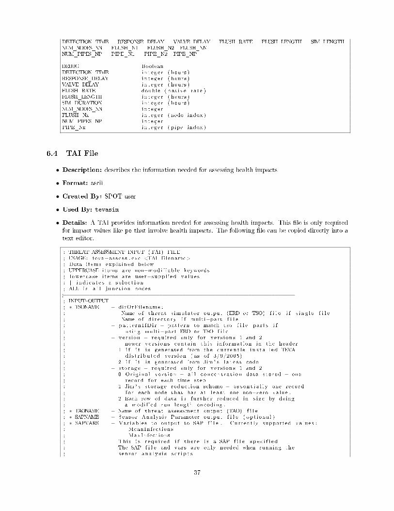
DETECTION_TIME RESPONSE_DELAY VALVE_DELAY FLUSH_RATE FLUSH_LENGTH SIM_LENGTHNUM_NODES_NN FLUSH_N1 FLUSH_N2 FLUSH_NNNUM_PIPES_NP PIPE_N1 PIPE_N2 PIPE_NP

DEBUG BooleanDETECTION_TIME in t e g e r ( hours )RESPONSE_DELAY in t e g e r ( hours )VALVE_DELAY in t e g e r ( hours )FLUSH_RATE double ( nat ive ra t e )FLUSH_LENGTH in t e g e r ( hours )SIM_DURATION in t e g e r ( hours )NUM_NODES_NN in t e g e rFLUSH_Nx in t e g e r ( node index )NUM_PIPES_NP in t e g e rPIPE_Nx in t e g e r ( pipe index )

6.4 TAI File

• Description: describes the information needed for assessing health impacts

• Format: ascii



• Details: A TAI provides information needed for assessing health impacts. This �le is only requiredfor impact values like pe that involve health impacts. The following �le can be copied directly into atext editor.

; THREAT ASSESSMENT INPUT (TAI) FILE; USAGE: teva−a s s e s s . exe <TAI f i l ename>; Data items exp la ined below; UPPERCASE items are non−mod i f i ab l e keywords; l owercase items are user−supp l i ed va lue s; | i n d i c a t e s a s e l e c t i o n; ALL i s a l l j unc t i on nodes;−−−−−−−−−−−−−−−−−−−−−−−−−−−−−−−−−−−−−−−−−−−−−−−−−−−−−−−−−−−−−−−−−−−−−−; INPUT−OUTPUT; ∗ TSONAME − dirOrFilename :; Name o f th r ea t s imu la to r output (ERD or TSO) f i l e i f s i n g l e f i l e; Name o f d i r e c t o r y i f multi−part f i l e; − pa t t e rn I fD i r − pattern to match t so f i l e par t s i f; us ing multi−part ERD or TSO f i l e; − ve r s i on − r equ i r ed only f o r v e r s i on s 1 and 2; newer v e r s i on s conta in t h i s in fo rmat ion in the header; 1 i f i t i s generated from the cu r r e n t l e i n s t a l l e d TEVA; d i s t r i b u t e d ve r s i on ( as o f 3/9/2005); 2 i f i t i s generated from Jim ' s l a t e s t code; − s t o rage − r equ i r ed only f o r v e r s i on s 1 and 2; 0 Or i g i na l v e r s i on − a l l concent ra t i on data s to r ed − one; r ecord f o r each time step; 1 Jim ' s s t o rage reduct ion scheme − e s s e n t i a l l y one record; f o r each node that has at l e a s t one non−zero value .; 2 Each row o f data i s f u r t h e r reduced in s i z e by doing; a modi f i ed run length encoding .; ∗ TAONAME − Name o f th r ea t assessment output (TAO) f i l e; ∗ SAPNAME − Sensor Ana lys i s Parameter output f i l e ( op t i ona l ); ∗ SAPVARS − Var iab l e s to output to SAP f i l e . Current ly supported va lue s :; MeanInfect ions; MaxInfect ions; This i s r equ i r ed i f the re i s a SAP f i l e s p e c i f i e d; The SAP f i l e and vars are only needed when running the; s enso r an a l y s i s s c r i p t s

37

;−−−−−−−−−−−−−−−−−−−−−−−−−−−−−−−−−−−−−−−−−−−−−−−−−−−−−−−−−−−−−−−−−−−−−−TSONAME cha r s t r i n gTAONAME cha r s t r i n gSAPNAME cha r s t r i n gSAPVARS varname_1 . . . varname_n;−−−−−−−−−−−−−−−−−−−−−−−−−−−−−−−−−−−−−−−−−−−−−−−−−−−−−−−−−−−−−−−−−−−−−−; DOSE−RESPONSE PARAMETERS; ∗ A − f unc t i on c o e f f i c i e n t; ∗ M − f unc t i on c o e f f i c i e n t; ∗ N − f unc t i on c o e f f i c i e n t; ∗ TAU − f unc t i on c o e f f i c i e n t; ∗ BODYMASS − exposed i nd i v i dua l body mass (Kg); ∗ NORMALIZE − Dose in mg/Kg ( ' yes ' ) or mg ( ' no ' ); ∗ BETA − Beta value f o r p rob i t dose re sponse model; ∗ LD50 − LD50 or ID50 value f o r the agent being s tud i ed; ∗ TYPE − e i t h e r PROBIT or OLD depending on the dose re sponse equat ion; to be used . I f i t i s PROBIT, only the LD50 and BETA va lues; need to be s p e c i f i e d , and i f i t i s OLD, the A, M, N, and TAU; va lue s need to be s p e c i f i e d . The BODYMASS and NORMALIZE; apply to both equat ions .;−−−−−−−−−−−−−−−−−−−−−−−−−−−−−−−−−−−−−−−−−−−−−−−−−−−−−−−−−−−−−−−−−−−−−−DR:A valueDR:M valueDR:N valueDR:TAU valueBODYMASS valueNORMALIZE YES|NODR:BETA valueDR:LD50 valueDR:TYPE prob i t | o ld

;−−−−−−−−−−−−−−−−−−−−−−−−−−−−−−−−−−−−−−−−−−−−−−−−−−−−−−−−−−−−−−−−−−−−−−; DISEASE MODEL; ∗ LATENCYTIME − time from exposed to symptoms ( hours ); ∗ FATALITYTIME − time from symptoms t i l l death ( hours ); ∗ FATALITYRATE − Fract ion o f exposed populat ion that d i e;−−−−−−−−−−−−−−−−−−−−−−−−−−−−−−−−−−−−−−−−−−−−−−−−−−−−−−−−−−−−−−−−−−−−−−LATENCYTIME valueFATALITYTIME valueFATALITYRATE value

;−−−−−−−−−−−−−−−−−−−−−−−−−−−−−−−−−−−−−−−−−−−−−−−−−−−−−−−−−−−−−−−−−−−−−−; EXPOSURE MODEL; ∗ DOSETYPE − TOTAL = to t a l i ng e s t ed mass; ∗ INGESTIONTYPE − DEMAND = ing e s t i o n p r obab i l i t y prop . to demand; ATUS RANDOM = ATUS ing e s t i o n model , random volume; s e l e c t i o n from volume curve; ATUS MEAN = ATUS ing e s t i o n model , mean volume o f va lue; FIXED5 RANDOM = 5 f i x ed i n g e s t i o n t imes (7am, 9 :30am,Noon , 3PM,6PM) ,; random volume s e l e c t i o n from volume curve; FIXED5 MEAN = 5 f i x ed i n g e s t i o n t imes (7am, 9 :30am,Noon , 3PM,6PM) ,

mean volume o f va lue; ∗ INGESTIONRATE − vo lumetr i c i n g e s t i o n ra t e ( l i t e r s /day ) − used f o r demand and

ATUS MEAN and FIXED5 MEAN;−−−−−−−−−−−−−−−−−−−−−−−−−−−−−−−−−−−−−−−−−−−−−−−−−−−−−−−−−−−−−−−−−−−−−−DOSETYPE TOTALINGESTIONTYPE DEMANDINGESTIONRATE value

;−−−−−−−−−−−−−−−−−−−−−−−−−−−−−−−−−−−−−−−−−−−−−−−−−−−−−−−−−−−−−−−−−−−−−−; POPULATION MODEL; ∗ POPULATION FILE − value i s the f i l ename that conta in s the node−based; populat ion . The format o f the f i l e i s s imply one l i n e; per node with the node id and the popuylat ion value; f o r that node .; ∗ POPULATION DEMAND − value i s the per cap i ta usage ra t e ( f low un i t s / person ) .; The populat ion w i l l be est imated by demand;−−−−−−−−−−−−−−−−−−−−−−−−−−−−−−−−−−−−−−−−−−−−−−−−−−−−−−−−−−−−−−−−−−−−−−

38

POPULATION FILE | DEMAND value;−−−−−−−−−−−−−−−−−−−−−−−−−−−−−−−−−−−−−−−−−−−−−−−−−−−−−−−−−−−−−−−−−−−−−−; DOSE OVER THRESHOLD MODEL; ∗ DOSE_THRESHOLDS − The dose over each thr e sho ld s p e c i f i e d w i l l be; computed and output to the TAO f i l e .; ∗ DOSE_BINDATA − S p e c i f i e s the endpoints o f b ins to t a l l y the number; o f people with a dose between the two endpoints .; Values can be e i t h e r does va lue s or re sponse va lue s −; Response va lue s are converted to Dose va lue s us ing the; dose−re sponse data s p e c i f i e d in t h i s f i l e and are i nd i c a t ed; on t h i s l i n e by the keyword RESPONSE. Dose va lue s are; IDENTIFIED by the keyword DOSE;−−−−−−−−−−−−−−−−−−−−−−−−−−−−−−−−−−−−−−−−−−−−−−−−−−−−−−−−−−−−−−−−−−−−−−DOSE_THRESHOLDS value1 . . . value_nDOSE_BINDATA (DOSE | RESPONSE) value1 . . . value_n

6.5 ERD File

• Description: provides a compact representation of simulation results.

• Format: binary

• Created By: tevasim

• Used By: tso2Impact

• Details: The simulation data generator produces four output �le containing the results of all threatsimulation scenarios. The database �les include an index �le (index.erd), hydraulics �le (hyd.erd) andwater quality �le (qual.erd). The �les are unformatted binary �le in order to save disk space andcomputation time. They are not readable using an ordinary text editor.

• Note: ERD �le format replaced the TSO and SDX �le format, created by previous versions of tevasim,to extend tevasim capability for multi-specie simulation using EPANET-MSX. While tevasim producesonly ERD �les (even for single specie simulation), tso2Impact accepts both ERD and TSO �le formats.

6.6 Sensor Placement File

• Description: describes one or more sensor placements

• Format: ascii

• Created By: sp

• Used By: evalsensor

• Details:

Lines in a sensor placement �le that begin with the '#' character are assumed to be comments.Otherwise, lines of this �le have the format

<sp-id> <number-of-sensors> <node-index-1> ...

The sensor placement ID is used to identify sensor placements in the �le. Sensor placements may havedi�ering numbers of sensors, so each line contains this information. The node indices map to values inthe Node File (p. 41).

39

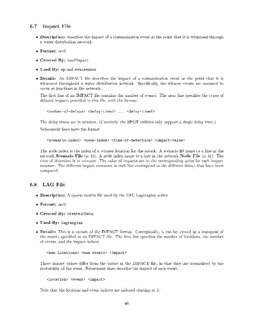
6.7 Impact File

• Description: describes the impact of a contamination event at the point that it is witnessed througha water distribution network.

• Format: ascii

• Created By: tso2Impact

• Used By: sp and evalsensor

• Details: An IMPACT �le describes the impact of a contamination event at the point that it iswitnessed throughout a water distribution network. Speci�cally, the witness events are assumed tooccur at junctions in the network.

The �rst line of an IMPACT �le contains the number of events. The next line speci�es the types ofdelayed impacts provided in this �le, with the format:

<number-of-delays> <delay-time1> ... <delay-timeN>

The delay times are in minutes. (Currently, the SPOT utilities only support a single delay time.)

Subsequent lines have the format

<scenario-index> <node-index> <time-of-detection> <impact-value>

The node index is the index of a witness location for the attack. A scenario ID maps to a line in thenetwork Scenario File (p. 41). A node index maps to a line in the network Node File (p. 41). Thetime of detection is in minutes. The value of impacts are in the corresponding units for each impactmeasure. The di�erent impact measures in each line correspond to the di�erent delays that have beencomputed.

6.8 LAG File

• Description: A sparse matrix �le used by the UFL Lagrangian solver

• Format: ascii

• Created By: createIPData

• Used By: lagrangian

• Details: This is a variant of the IMPACT format. Conceptually, it can be viewed as a transpose ofthe matrix speci�ed in an IMPACT �le. The �rst line speci�es the number of locations, the numberof events, and the impact values:

<num-locations> <num-events> <impact>

These impact values di�er from the values in the IMPACT �le, in that they are normalized by theprobability of the event. Subsequent lines describe the impact of each event:

<location> <event> <impact>

Note that the location and event indices are indexed starting at 1.

40

6.9 Scenario File

• Description: The scenario �le provides auxiliary information about each contamination incident.

• Format: ascii


• Used By: evalsensor

• Details: Each line of this �le has the format:

<node-index> <EPANET-ID> <source-type> <source-start-time> <source-stop-time> <source-strength>

The node index maps to the networkNode File (p. 41), and the EPANET ID provides this information(redundantly). The scenario start and stop are in minutes, and these values are relative to the startof the EPANET simulation. The source type is the injection mode for an attack, e.g., �ow-paced or�xed-concentration. The source strength is the concentration of contaminant at the attack source.

6.10 Node File

• Description: provides a mapping from the indices used for sensor placement to the junction IDs usedwithin EPANET

• Format: ascii


• Used By: evalsensor and sensor placement solvers

• Details: The node �le provides a mapping from the indices used for sensor placement to the IDs usedwithin EPANET. Each line of this �le has the format:

<node-index> <EPANET-ID>

This mapping is generated by tso2Impact (p. 76), and all sensor placement solvers subsequently usethe node indices internally.

6.11 Sensor Placement Con�guration File

• Description: a con�guration �le used to de�ne a sensor placement problem

• Format: ascii

• Created By: sp

• Used By: createIPData

• Details: The sensor placement con�guration �le is generated by the sp (p. 65) solver interface, and itcontains all of the information that is needed to de�ne a sensor placement problem. The �le has thefollowing format:

<number-of-junctions> <response-delay>

<number-of-goals>

<goal-name> <goal-filename> <compression-threshold> <compression-percentage> <attack-collapse-flag>\

<number-of-measures>\

41

<measure-name> ... <measure-name> <objective-flag>\

<bound-value> ... <bound-value>

<fixed-sensor-placements>

<invalid-sensor-placements>

<cost-values>

The values in this �le correspond to the command-line arguments of the sp (p. 65) solver. Compressionthreshold or percentage refers to node aggregation values. The attack-collapse-�ag is a 0 or 1 value inthe con�guration �le, indicating whether compression/aggregation can make an attack trivial (singlesupernode equivalent to no detection). The <�xed-sensor-placements>, <invalid-sensor-placements>and <cost-values> data sets are simply an import of the data from the corresponding �les that arespeci�ed within the sp (p. 65) solver interface.

6.12 Sensor Placement Costs File

• Description: speci�es the costs for installing sensors at di�erent junctions throughout a network

• Format: ascii


• Used By: sp


<EPANET-ID> <cost>

Junctions not explicitly enumerated in this �le are assumed to have zero cost unless the ID '__-default__' is speci�ed. For example:

__default 1.0

This example would specify that all un-enumerated junctions have a cost of 1.0.

6.13 Placement Locations File

• Description: speci�es whether sensor placements are �xed and whether locations are feasible sensorplacement

• Format: ascii


• Used By: sp


<keyword> <EPANET-ID> ... <EPANET-ID>

The valid keywords are feasible, infeasible, �xed and un�xed. These keywords correspond to twosemantic states for each location: (1) the feasibility of sensor placement and (2) whether a sensorplacement is forced. The semantics of these keywords are as follows:

� feasible - the speci�ed locations are feasible and un�xed

� infeasible - the speci�ed locations are infeasible and un�xed

42

� �xed - the speci�ed locations are constrained to contain a sensor (�xed and feasible)

� un�xed - the speci�ed locations are not constrained to contain a sensor (un�xed and feasible)

The locations are EPANET-IDs from the network model. Additionally, the keyword ALL or ∗ can beused to specify that all network locations are to be processed.

A location �le is processed sequentially. The initial state is that all locations are feasible and un�xed.Subsequently, each line updates the state of the locations, given the state de�ned by the previous linesof this �le. For example, the �le:

infeasible ALL

feasible A B C

makes all locations infeasible except for locations A, B and C. Similarly

fixed ALL

feasible A B C

makes all locations �xed except for locations A, B and C; the feasible keyword has the same semanticsas the un�xed keyword.

6.14 Sensor Class File

• Description: contains false-negative probabilities for di�erent types of sensors

• Format: ascii


• Used By: sp

• Details: The �le has format:

<class id> <false negative probability>

<class id> <false negative probability>

....

For example, the following �le de�nes a failure class 1, with a false negative rate of 25 percent, and a failureclass 2 with a false negative rate of 50 percent:

1 0.25

2 0.5

....

6.15 Junctions Class File

• Description: provides the mapping from EPANET junction IDs to failure classes

• Format: ascii

• Created By: EPANET user

• Used By: sp

43

• Details: When a sensor class �le is being used, the "junction class" �le provides the mapping fromjunction (node) id's to failure classes. The format of this �le is:

<node id> <failure class>

<node id> <failure class>

....

For example, supposing that junction 1 is of class 2, junction 2 is of class 1, and junction 3 is of class 1:

1 2

2 1

3 1

....

44

Bibliography

[1] R. Bahadur, W. B. Samuels, W. Grayman, D. Amstutz, and J. Pickus. Pipelinenet: A model formonitoring introduced contaminants in a distribution system. In Proc. World Water and Environmental

Resources Congress. ASCE, 2003.

[2] J. Berry, R. D. Carr, W. E. Hart, V. J. Leung, C. A. Phillips, and J.-P. Watson. Designing contaminationwarning systems for municipal water networks using imperfect sensors. Journal of Water Resources

Planning and Management, 135(4):253�263, 2009.

[3] J. Berry, L. Fleischer, W. E. Hart, C. A. Phillips, and J.-P. Watson. Sensor placement in municipalwater networks. J. Water Resources Planning and Management, 131(3):237�243, 2005.

[4] J. Berry, W. E. Hart, C. A. Phillips, J. Uber, and T. Walski. Water quality sensor placement in waternetworks with budget constraints. In Proc. World Water and Environment Resources Conference, 2005.

[5] J. Berry, W. E. Hart, C. E. Phillips, J. G. . Uber, and J.-P. Watson. Sensor placement in municiple waternetworks with temporal integer prog ramming models. J. Water Resources Planning and Management,132(4):218�224, 2006.

[6] J. W. Berry, W. E. Hart, and C. A. Phillips. Scalability of integer programming computations for sensorplacement in municipal water networks. In Proc. World Water and Environmental Resources Congress.ASCE, 2005.

[7] R. Carr, H. Greenberg, W. Hart, G. Konjevod, E. Lauer, H. Lin, T. Morrison, and C. Phillips. Robustoptimization of contaminant sensor placement for community water systems. Mathematical Program-

ming, 107(1):337�356, 2006.

[8] J. R. Chastain, Jr. A Heuristic Methodology for Locating Monitoring Stations to Detect Contamination

Events in Potable Water Distribution Systems. PhD thesis, University of South Florida, 2004.

[9] W. E. Hart, J. Berry, R. Murray, C. A. Phillips, L. A. Riesen, and J.-P. Watson. SPOT: A sensorplacement optimization toolkit for drinking water contaminant warning system design. Technical ReportSAND2007-4393, Sandia National Laboratories, 2007.

[10] K. Klise, C. Phillips, and R. Janke. Two-tiered sensor placement using skeletonized water distributionnetwork models. in review.

[11] P. Mirchandani and R. Francis, editors. Discrete Location Theory. John Wiley and Sons, 1990.

[12] K. Morley, R. Janke, R. Murray, and K. Fox. Drinking water contamination warning systems: Waterutilities driving water research. J. AWWA, pages 40�46, 2007.

[13] R. Murray, J. Berry, and W. E. Hart. Sensor network design for contamination warning systems: Toolsand applications. In Proc. AWWA Water Security Congress, 2006.

[14] R. Murray, J. Uber, and R. Janke. Modeling acute health impacts resulting from ingestion of contami-nated drinking water. J. Water Resources Planning and Management: Special Issue on Drinking Water

Distribution Systems Security, 2006.

[15] A. Ostfeld and E. Salomons. Optimal layout of early warning detection stations for water distributionsystems security. J. Water Resources Planning and Management, 130(5):377�385, 2004.

[16] A. Ostfeld, J. G. Uber, E. Salomons, J. W. Berry, W. E. Hart, C. A. Phillips, J.-P. Watson, G. Dorini,P. Jonkergouw, Z. Kapelan, F. di Pierro, S.-T. Khu, D. Savic, D. Eliades, M. Polycarpou, S. R. Ghimire,B. D. Barkdoll, R. Gueli, J. J. Huang, E. A. McBean, W. James, A. Krause, J. Leskovec, S. Isovitsch,J. Xu, C. Guestrin, J. VanBriesen, M. Small, P. Fischbeck, A. Preis, M. Propato, O. Piller, G. B.

45

Trachtman, Z. Y. Wu, and T. Walski. The battle of the water sensor networks (BWSN): A designchallenge for engineers and algorithms. J Water Resources Planning and Management, 134(6):556�568,Nov/Dec 2008.

[17] R. T. Rockafellar and S. Uryasev. Conditional value-at-risk for general loss distributions. J. of Bankingand Finance, 26(7):1443�1471, 2002.

[18] L. A. Rossman. The EPANET programmer's toolkit for analysis of water distribution systems. InProceedings of the Annual Water Resources Planning and Management Conference, 1999. Available athttp://www.epa.gov/nrmrl/wswrd/dw/epanet.html.

[19] F. Shang, J. Uber, and L. Rossman. Epanet mutli-species extension user's manual. Technical ReportEPA/600/S-07/021, USEPA, 2011.

[20] N. Topaloglou, H. Vladimirou, and S. Zenios. CVaR models with selective hedging for internationalasset allocation. J. of Banking and Finance, (26):1535�1561, 2002.

[21] G. B. Trachtman. A �strawman� common sense approach for water quality sensor site selection. InProc. 8th Annual Water Distribution System Analysis Symposium, 2006.

[22] USEPA. WaterSentinel System Architecture. Technical report, U.S. Environmental Protection Agency,2005.

[23] J.-P. Watson, H. J. Greenberg, and W. E. Hart. A multiple-objective analysis of sensor placementoptimization in water networks. In Proc. World Water and Environment Resources Conference, 2004.

[24] J.-P. Watson, W. E. Hart, and R. Murray. Formulation and optimization of robust sensor placementproblems for contaminant warning systems. In Proc. Water Distribution System Symposium, 2006.

46

http://www.epa.gov/nrmrl/wswrd/dw/epanet.html

A Unix Installation

The TEVA-SPOT Toolkit employs the integer programming solvers provided by the Acro software. Thisexample illustrates how to build both SPOT and Acro. After release 2.1.1, SPOT and Acro need to be builtand con�gured separately.

A.1 Downloading

There are several ways that SPOT and Acro can be downloaded. First, these two packages can be downloadeddirectly from the subversion repository using the svn command, which is commonly available on Linuxcomputers. The SPOT and Acro subversion repositories support anonymous checkouts, so you should notneed passwords. The following steps checkout the latest trunk version of these packages:

svn checkout -q https://software.sandia.gov/svn/public/acro/acro-pico/trunk acro-pico

svn checkout -q https://software.sandia.gov/svn/teva/spot/spot/trunk spot

Alternatively, recent tarballs of the acro-pico and spot software can be downloaded from the Acro downloadsite and SPOT download site. Once downloaded, these compressed tarballs can be expanded using the tarcommand:

tar xvfz filename.tar.gz

A.2 Con�guring and Building

Acro can be con�gured using the standard build syntax:

cd acro-pico

./setup

autoreconf -i -f

./configure

make

This builds libraries in acro-pico/lib, along with executables in acro-pico/bin. The setup command bootstrapsthe con�guration process with �les from the bootstrap directory.

SPOT can be con�gured and built in a similar manner:

cd spot

./setup

autoreconf -i -f

./configure

make

47

B Data Requirements

The Threat Ensemble Vulnerability Assessment Sensor Placement Optimization Tool, TEVA-SPOT, is asoftware product and decision-making process developed by EPA's TEVA Research program to assist indetermining the best location for sensors in a distribution system. In the past, the TEVA-SPOT softwarehas been applied by EPA sta� using models and data provided by utilities. In some cases, signi�cantimprovements in the models have been made in order to bring them up to the standards required by theTEVA-SPOT software. In order to streamline the application of TEVA-SPOT, this document was developedto describe the requirements and steps that utilities must follow to participate in the TEVA program and/oruse TEVA-SPOT.

Table 1 summarizes the data and information required for a water utility to use TEVA-SPOT; each com-ponent is described in more detail in the text. In addition to having an appropriate utility network model,utilities will need to make decisions about the nature of the Contamination Warning System they are de-signing and the types of security incidents that they would like to detect.

Table 1. Information and data required for utilities to design sensor networks using TEVA-SPOT.

INFORMATION AND DATANEEDED FOR SENSORPLACEMENT

DESCRIPTION

Utility Network Model The model (e.g. EPANET input �le) should be up-to-date, capa-ble of simulating operations for a 7-10 day period, and calibratedwith �eld data.

Sensor Characteristics Type of sensors or sampling program, detection limits, and (ifapplicable) event detection system

Design Basis Threat Data describing type of event that the utility would like to beable to detect: speci�c contaminants, behavior of adversary, andcustomer behavior

Performance Measures Utility speci�c critical performance criteria, such as time to de-tection, number of illnesses, etc.

Utility Response Plan for response to a positive sensor reading, including total timerequired for the utility to limit further public exposure.

Potential Sensor Locations List of all feasible locations for placing sensors, including associ-ated model node/junction.

UTILITY NETWORK MODEL

The TEVA-SPOT software relies upon an EPANET hydraulic model of the network as the mechanismfor calculating the impacts resulting from contamination incidents. Therefore, an acceptable model of thedistribution system is needed in order to e�ectively design the sensor system. The following sub-sectionsdescribe the various issues/characteristics of an acceptable hydraulic model for use within TEVA-SPOT.

EPANET Software Requirement TEVA-SPOT uses EPANET, a public domain water distribution sys-tem modeling software package. In order to utilize TEVA-SPOT, existing network models that were notdeveloped in EPANET must be converted to and be demonstrated to properly operate within EPANET (Ver-sion 2.00.11). Most commercial software packages utilize the basic EPANET calculation engine and containa conversion tool for creating an EPANET input �le from the �les native to the commercial package. Theuser may encounter two potential types of problems when they attempt to make the conversion: (1) somecommercial packages support component representations that are not directly compatible with EPANETsuch as representation of variable speed pumps. The representation of these components may need to be

48

modi�ed in order to operate properly under EPANET; (2) additionally, the conversion programs developedby the commercial software vendors may also introduce some unintended representations within EPANETthat may require manual correction. Following conversion, the output from the original model should becompared with the EPANET model output to ensure that the model results are the same or acceptably close(see section on Model Testing).

Extended Period Simulation TEVA-SPOT uses both the hydraulic and water quality modeling portionsof EPANET. In order to support the water quality modeling, the model must be an extended period simula-tion (EPS) that represents the system operation over a period of several days. Typically a model that usesrules to control operations (e.g., turn pump A on when the water level in tank B drops to a speci�ed level)are more resilient and amenable to long duration runs than are those that use controls based solely on timeclocks. Model output should be examined to ensure that tank water levels are not systematically increasingor decreasing over the course of the run since that will lead to unsustainable situations.

The required length of simulation depends on the size and operation of the speci�c water system. However,in general, the length of the simulation should re�ect the longest travel times from a source to customernodes. This can be calculated by running the EPANET model for water age and determining the higherwater age areas. In determining the required simulation length, small dead-ends (especially those with zerodemand nodes) can be ignored. Typically a run length of 7 to 10 days is required for TEVA-SPOT thoughshorter periods may su�ce for smaller systems and longer run times required for larger or more complexsystems.

Seasonal Models In most cases, water security incidents can take place at any time of the day or any seasonof the year. As a result, sensor systems should be designed to operate during one or more representativeperiods in the water system. It should be noted that this di�ers signi�cantly from the normal design criteriafor a water system where pipes are sized to accommodate water usage during peak seasons or during unusualevents such as �res. In many cases, the only available models are representative of these extreme cases andgenerally, modi�cations to such models should be made to re�ect a broader time period prior to use withTEVA-SPOT. Speci�c guidance on selecting models is provided below:

• Optimal situation: the utility has multiple models representing average conditions throughout theyear, typical higher demand case (e.g., average summer day) and typical lower demand case (e.g.,average winter day).

• Minimal situation: the utility has a single model representing relatively average conditions through-out the year.

• Situations to avoid: the utility has a single model representing an extreme case (e.g., maximum daymodel).

• Exceptions: (1) If a sensor system is being designed to primarily monitor a water system during aspeci�c event such as a major annual festival, then one of the models should re�ect conditions duringthat event; and (2) If the water system experiences little variation in water demand and water systemoperation over the course of the year, then a single representative model would su�ce.

Model Detail A su�cient amount of detail should be represented in the model for use within TEVA-SPOT.This does not mean that an all-pipes model is required nor does it mean that a model that only representstransmission lines would su�ce. At a minimum, all parts of the water system that are considered criticalfrom a security standpoint should be included in the model, even if they are on the periphery of the system.The following guidance drawn from the Initial Distribution System Evaluation (IDSE) Guidance Manual ofthe Final Stage 2 Disinfectants and Disinfection Byproducts Rule provides a reasonable lower limit for thelevel of detail required for a TEVA-SPOT analysis (USEPA, 2006).

Most distribution system models do not include every pipe in a distribution system. Typically, small pipesnear the periphery of the system and other pipes that a�ect relatively few customers are excluded to agreater or lesser extent depending on the intended use of the model. This process is called skeletonization.

49

Models including only transmission networks (e.g. pipes larger than 12 inches in diameter only) are highlyskeletonized while models including many smaller diameter distribution mains (e.g. 4 to 6 inches in diameter)are less skeletonized. In general, water moves quickly through larger transmission piping and slower throughthe smaller distribution mains. Therefore, the simulation of water age or water quality requires that thesmaller mains be included in the model to fully capture the residence time and potential water qualitydegradation between the treatment plant and the customer. Minimum requirements for physical systemmodeling data for the IDSE process are listed below.

• At least 50 percent of total pipe length in the distribution system.

• At least 75 percent of the pipe volume in the distribution system.

• All 12-inch diameter and larger pipes.

• All 8-inch diameter and larger pipes that connect pressure zones, mixing zones from di�erent sources,storage facilities, major demand areas, pumps, and control valves, or are known or expected to besigni�cant conveyors of water.

• All 6-inch diameter and larger pipes that connect remote areas of a distribution system to the mainportion of the system or are known or expected to be signi�cant conveyors of water.

• All storage facilities, with controls or settings applied to govern the open/closed status of the facilitythat re�ect standard operations.

• All active pump stations, with realistic controls or settings applied to govern their on/o� status thatre�ect standard operations.

• All active control valves or other system features that could signi�cantly a�ect the �ow of water throughthe distribution system (e.g., interconnections with other systems, pressure reducing valves betweenpressure zones).

Model Demands The movement of water through a distribution system is largely driven by water demands(consumption) throughout the system. During higher demand periods, �ows and velocities generally increaseand vice versa. Demands are usually represented within a model as average or typical demands at most nodesand then (a) global or regional demand multipliers are applied to all nodes to represent periods of higheror lower demand, and (b) temporal demand patterns are applied to de�ne how the demands vary over thecourse of a day. In some models, demands within a large area have been aggregated and assigned to a centralnode. In building a model for use with TEVA-SPOT, rather than aggregating the demands and assigningthem to only a few nodes, each demand should be assigned to the node that is nearest to the actual point ofuse. Both EPANET and most commercial software products allow the user to assign multiple demands to anode with di�erent demands assigned to di�erent diurnal patterns. For example, part of the demand at anode could represent residential demand and utilize a pattern representative of residential demand. Anotherportion of the demand at the same node may represent commercial usage and be assigned to a representativecommercial diurnal water use pattern. TEVA-SPOT supports either a single demand or multiple demandsassigned to nodes.

Model Calibration/Validation Calibration is the process of adjusting model parameters so that predictedmodel outputs generally re�ect the actual behavior of the system. Validation is the next step after calibration,in which the calibrated model is compared to independent data sets (i.e., data that was not used in thecalibration phase) in order to ensure that the model is valid over wider range of conditions. There are noformal standards in the water industry concerning how closely the model results need to match �eld resultsnor is there formal guidance on the amount of �eld data that must be collected. Calibration methods thatare frequently used include roughness (c-factor) tests, hydrant �ow tests, tracer tests and matching modelresults over extended periods for pressure, �ow and tank water levels to �eld data collected from SCADAsystems or special purpose data collection e�orts.

50

The IDSE Guidance Manual stipulates the following minimum criteria in order to demonstrate calibration.�The model must be calibrated in extended period simulation for at least a 24-hour period. Because storagefacilities have such a signi�cant impact upon water age and reliability of water age predictions throughoutthe distribution system, you must compare and evaluate the model predictions versus the actual waterlevels of all storage facilities in the system to meet calibration requirements.� For TEVA-SPOT application,the water utility should calibrate the model to a level that they are con�dent that the model adequatelyre�ects the actual behavior of the water system being represented by the model. Some general guidelines forcalibration/validation are shown below:

• If the model has been in operation actively and for several years and has been applied successfullyin a variety of extended period simulation situations, then further substantial calibration may notbe necessary. However, even in this case, it is prudent to demonstrate the validity of the model bycomparing the model results to �eld measurements such as time-varying tank water levels and/or �eldpressure measurements.

• If the model has been used primarily for steady state applications, then further calibration/validationemphasizing extended period simulation is needed.

• If the model has been recently developed and not undergone signi�cant application, then a formalcalibration/validation process is needed.

Model Tanks Tank mixing models: Most water distribution system models use a �complete mix� tankrepresentation that assumes that tanks are completely and instantaneously mixed. EPANET (and mostcommercial modeling software models) allow for alternative mixing models such as last in-�rst out (LIFO),�rst in-�rst out (FIFO), and compartment models. If a utility has not previously performed water qualitymodeling, they may not have determined the most appropriate tank mixing model for each tank. Since thetank mixing model can a�ect contaminant modeling and thus the sensor placement decisions, tank mixingmodels should be speci�ed in the EPANET model input �les.

Model Testing The �nal step in preparing the model for use in TEVA-SPOT is to put the model througha series of candidate tests. Following is a list of potential tests that should be considered.

• If the model was developed and applied using a software package other than EPANET, then followingits conversion to EPANET, the original model and the new EPANET model should be run in parallelunder EPS and the results compared. The models should give virtually the same results or very similarresults. Comparisons should include tank water levels and �ows in major pipes, pumps and valves overthe entire time period of the simulation. If there are signi�cant di�erences between the two models,then the EPANET model should be modi�ed to better re�ect the original model or di�erences shouldbe explained and justi�ed.

• The EPANET model should be run over an extended period (typically 1 to 2 weeks) to test forsustainability. In a sustainable model, tank water levels cycle over a reasonable range and do notdisplay any systematic drops or increases. Thus, the range of calculated minimum and maximumwater levels in all tanks should be approximately the same in the last few days of the simulation asthey were in the �rst few days. Typically, a sustainable model will display results that are in dynamicequilibrium in which temporal tank water level and �ow patterns will repeat themselves on a daily (orother periodic) basis.

• If the water system has multiple sources, then the source tracing feature in EPANET should be usedto test the movement of water from each source. In most multiple source systems, operators generallyhave a good idea as to how far the water from each source travels. The model results should be shownto the knowledgeable operators to ensure that the model is operating in a manner that is compatiblewith their understanding of the system.

• The model should be run for a lengthy period (1 to 2 weeks) using the water age option in EPANETin order to determine travel times. Since the water age in tanks is not usually known before modeling,

51

a best guess (not zero hours) should be used to set an initial water age for each tank. Then after thelong run of the model, a graph of calculated water age should be examined for each tank to ensurethat it has reached a dynamic equilibrium and is still not increasing or decreasing. If the water ageis still systematically increasing or decreasing, then the plot of age for each tank should be visuallyextrapolated to estimate an approximate �nal age and that value should be reinserted in the model asan initial age, and the model rerun for the extended period. The model output of water age shouldthen be investigated for reasonableness, e.g., are there areas where water age seems unreasonably high?This exercise will also help to de�ne a reasonable upper limit for the duration of the model run to beused in the TEVA-SPOT application.

Following these test runs, any identi�ed modi�cations should be made in the model to ensure that themodel will operate properly under TEVA-SPOT. Many utilities will not be able to make all of the abovemodi�cations to their network model. In that case, TEVA-SPOT can still be applied; however the overallaccuracy of the results will be questionable and should only be considered applicable to the system asdescribed by the model.

SENSOR CHARACTERISTICS

The TEVA-SPOT analysis requires some assumptions about the detection characteristics of the sensors. Inparticular, the sensor type, detection limit, and accuracy need to be speci�ed. For example, the analysis canspecify a contaminant-speci�c detection limit that re�ects the ability of the water quality sensors to detectthe contaminant. Alternatively, the analysis can assume perfect sensors that are capable of detecting allnon-zero concentrations of contaminants with 100

In order to quantify detection limits for water quality sensors, the utility must indicate the type of waterquality sensor being used, as well as the disinfection method used in the system. Generally, water qualitysensors are more sensitive to contaminant introduction with chlorine disinfection than with chloramine. Asa result, contaminant detection limits may need to be increased in the design of a sensor network for achloraminated system.

Ongoing pilot studies for EPA's Water Security Initiative use a platform of water quality sensors, includingfree chlorine residual, total organic carbon (TOC), pH, conductivity, oxidation reduction potential (ORP),and turbidity (USEPA, 2005b). The correlation between contaminant concentration and the change in thesewater quality parameters can be estimated from experimental data, such as pipe loop studies (Hall et al.,2007; USEPA, 2005c). Of these parameters, chlorine residual and TOC seem to be most likely to detect awide range of contaminants.

Detection limits for water quality sensors can be de�ned in terms of the concentration that would change oneor more water quality parameters enough that the change would be detected by an event detection system(for example, Cook et al., 2005; McKenna, Wilson and Klise, 2006) or a water utility operator. A utilityoperator may be able to recognize a possible contamination incident if a change in water quality is signi�cantand rapid. For example, if the chlorine residual decreased by 1 mg/L, the conductivity increased by 1505Sm/cm, or TOC increased by 1 mg/L.

DESIGN BASIS THREAT

A design basis threat identi�es the type of threat that a water utility seeks to protect against when designinga CWS. In general, a CWS is designed to protect against contamination threats; however, there are a largenumber of potentially harmful contaminants and a myriad of ways in which a contaminant can be introducedinto a distribution system. Some utilities may wish to design a system that can detect not only high impactincidents, but also low impact incidents that may be caused by accidental back�ow or cross-connections. Itis critical for a water utility to agree upon the most appropriate design basis threat before completing thesensor network design.

Contamination incidents are speci�ed by the type of contaminant(s), the quantity of contaminant, thelocation(s) at which the contaminant is introduced into the water distribution system, the time of day of

52

the introduction, and the duration of the contaminant introduction. Given that it is di�cult to predict thebehavior of adversaries, it is unlikely that a water utility will know, with any reasonable level of certainty,the speci�c contamination threats that they may face. The TEVA-SPOT approach assumes that most ofthese parameter values cannot be known precisely prior to an incident; therefore, the modeling process musttake this uncertainty into account.

As an example, probabilities are assigned to each location in a distribution system indicating the likelihoodthat the contaminant would be introduced at that location. The default assumption is that each location isequally likely to be selected by an adversary (each has the same probability assigned to it). A large numberof contamination incidents (an ensemble of incidents) are then simulated and sensor network designs areselected based on how well they perform for the entire set of incidents. Based on their completed vulnerabilityassessment and other security related studies, a utility may have some knowledge or preconceived ideas thatwill assist in re�ning these assumptions. Some speci�c questions to consider are listed below:

• Are there certain locations that should be assigned higher probabilities? Should all nodes be consideredas possible introduction sites or only nodes with consumer demand?

• Should utility infrastructure sites, such as storage tanks, be considered as potential contaminationentry locations?

• Are there speci�c contaminants of concern to this utility?

PERFORMANCE MEASURES

The TEVA-SPOT software utilizes an optimization model that selects the best sensor design in order tomeet a speci�c set of performance measures. These measures are also sometimes referred to as objectives ormetrics. There are several performance measures that are currently supported by TEVA-SPOT including:

• the number of persons who become ill from exposure to a contaminant

• the percentage of incidents detected

• the time of detection

• the length of pipe contaminated

Although it requires more time and input from the user, TEVA-SPOT can also consider multiple objectivesin its analysis. If the water utility has any preferences in the area of performance measures, they shouldspecify which of the above measures should be used and the relative importance (weight) to be assigned toeach measure. If there are other quantitative measures that they wish to be considered, these should bespeci�ed.

UTILITY RESPONSE

The TEVA-SPOT analysis uses the concept of �response times� in the analysis of the e�ectiveness of a sensorsystem. Response time is an aggregate measure of the total time between the indication of a contaminationincident (e.g., detection of an unusual event by a sensor system) and full implementation of an e�ectiveresponse action such that there are no more consequences. The following response activities are likelyfollowing sensor detection (USEPA, 2004; Bristow and Brumbelow, 2006):

• Credibility determination: integrating data to improve con�dence in detection; for example, by lookingfor additional sensor detections or detection by a di�erent monitoring strategy, and checking sensormaintenance records.

• Veri�cation of contaminant presence: collection of water samples in the �eld, �eld tests and/or labo-ratory analysis to screen for potential contaminants.

53

• Public warning: communication of public health notices to prevent further exposure to contaminatedwater.

• Utility mitigation: implementing appropriate utility actions to reduce likelihood of further exposure,such as isolation of contaminated water in the distribution system or other hydraulic control options.

• Medical mitigation: public health actions to reduce the impacts of exposure, such as providing medicaltreatment and/or vaccination.

Past analyses have shown that the bene�ts of a contaminant warning system (CWS) are very dependent ona rapid response time. Typically, the TEVA-SPOT analysis assesses a range of response times between 0 and24 hours. A zero hour response time is obviously infeasible but is usually analyzed in TEVA-SPOT as thebest-case scenario and thus the maximum bene�ts that can be associated with a CWS. Water utilities shouldassess their own emergency response procedures and their acceptable risk tolerance in terms of false negativeand false positive responses in order to de�ne a range of response times to be used in the TEVA-SPOTanalysis.

POTENTIAL SENSOR LOCATIONS

TEVA-SPOT searches potential sensor locations to determine those set of locations (nodes) that will resultin the optimal performance measure for a particular number of sensors. Utilities can choose to consider allnodes as potential sensor locations or to limit the search to a subset of speci�ed nodes.

The primary physical requirements for locating sensors at a particular location are accessibility, electricity,physical security, data transmission capability, sewage drains, and temperatures within the manufacturerspeci�ed range for the instrumentation (ASCE, 2004). Accessibility is required for installation and main-tenance of the sensor stations. Electricity is necessary to power sensors, automated sampling devices, andcomputerized equipment. Physical security protects the sensors from natural elements and vandalism ortheft. Data transmission is needed to transmit sensor signals back to a centralized SCADA database, andcan be accomplished through a variety of solutions including digital cellular, private radio, land-line, or �ber-optic cable. Sewage drains are required to dispose of water and reagents from some sensors. Temperaturecontrols may be needed to avoid freezing or heat damage.

Most drinking water utilities can identify many locations satisfying the above requirements, such as pumpingstations, tanks, valve stations, or other utility-owned infrastructure. Many additional locations may meetthe above requirements for sensor locations or could be easily and inexpensively adapted. Other utilityservices, such as sewage systems, own sites that likely meet most of the requirements for sensor locations(e.g., collection stations, wastewater treatment facilities, etc.). In addition, many publicly-owned sites couldbe easily adapted, such as �re and police stations, schools, city and/or county buildings, etc. Finally, manyconsumer service connections would also meet many of the requirements for sensor placement, although theremay be di�culties in securing access to private homes or businesses. Nevertheless, the bene�t of using theselocations may be worth the added cost. Compliance monitoring locations may also be feasible sites.

The longer the list of potential sensor sites, the more likely one is to design a high-performing CWS. Typically,the TEVA-SPOT analysis will consider two or three subsets of nodes. For example, the set of all nodes inthe model, the set of all publicly-owned facilities, and the set of all water utility owned facilities. The utilityshould develop a list of the (EPANET) node numbers associated with the facilities that they would like tohave considered as potential sensor locations. Multiple lists indicating di�erent subsets (such as water utilityowned, publicly owned, etc.) may also be speci�ed.

POPULATION

In TEVA-SPOT analyses, the most commonly used performance measure for sensor placement is the numberof persons made ill following exposure to contaminated drinking water. In order to estimate health impacts,information is needed on the population at each node. There are a variety of methods that can be used toestimate nodal population.

54

• The simplest method is to assume a constant relationship between demand assigned to a node andthe population for that node. This method is most appropriate for a homogeneous, largely residentialarea. If a water demand-based population method is to be used, the total population calculated by themodel using a per capita water usage rate needs to be veri�ed with the population served consideringbilling records.

• Alternatively, if the number of service connections and types of service connections (i.e. residential,commercial, industrial, etc.) are known for each node, then this information can be used to estimatepopulation.

• A third alternative involves independent determination of population based on census data. If the useof a census-based population is desired, the population associated with each non-zero demand nodeof the model needs to be determined using the census data and GIS software. The resulting totalpopulation needs to be veri�ed with the population served by the water system.

If the second or third method is used to estimate nodal population, a �le (text �le or spreadsheet) shouldbe developed listing model node numbers and the population assigned to that node.

For more information about applying the TEVA-SPOT methodology, see Murray et al. (2007) or visit theEPA website http://www.epa.gov/nhsrc/water/teva.html.

ADDITIONAL READING

American Society of Civil Engineers (ASCE), 2004. Interim Voluntary Guidelines for Designing an OnlineContaminant Monitoring System.

Berry, J. et al, 2005. Sensor Placement in Municipal Water Networks. Jour. Wat. Res. Plan. Manag. 131(3): 237-243.

Berry, J. et al, 2006. Sensor Placement in Municipal Networks with Temporal Integer Programming Models.Jour. Wat. Res. Plan. Manag. 132(4): 218-224.

Bristow, E. and Brumbelow, K., 2006. Delay between sensing and response in water contamination events.Jour. Infrastructure Systems, p. 87-95.

Cook, J. et al, 2005. Decision Support System for Water Distribution System Monitoring for HomelandSecurity. Proceedings of the AWWA Water Security Congress, Oklahoma City.

Hall, J. et al, 2007. On-line Water Quality Parameters as Indicators of Distribution System Contamination.Jour. AWWA, 99:1:66-77.

McKenna, S. et al, 2006. Detecting Changes in Water Quality. Jour. AWWA, to appear.

Murray, R., Janke, R. Hart, W., Berry, J., Taxon, T. and Uber, J, 2007. A sensor network design decisionframework for Contamination Warning Systems. Submitted to Jour. AWWA.

U. S. Environmental Protection Agency, 2004. Response Protocol Toolbox: Plan-ning for and Responding to Drinking Water Contamination Threats and Incidents.http://www.epa.gov/safewater/watersecurity/pubs/rptb_response_guidelines.pdf

U. S. Environmental Protection Agency, 2005a. Review of State-of-the-Art Early Warning Systems forDrinking Water.

U. S. Environmental Protection Agency, 2005b. WaterSentinel System Architecture.http://epa.gov/watersecurity/pubs/watersentinel_system_architecture.pdf

U. S. Environmental Protection Agency, 2005c. WaterSentinel Online Water Quality Monitoring as anIndicator of Contamination. http://epa.gov/watersecurity/pubs/watersentinel_wq_monitoring.pdf

55

U. S. Environmental Protection Agency, 2006. Initial Distribution System Evaluation GuidanceManual for the Final Stage 2 Disinfectants and Disinfection Byproducts Rule. EPA 815-B-06-002.http://www.epa.gov/safewater/disinfection/stage2/pdfs/guide_idse_full.pdf

56

C Executable evalsensor

C.1 Overview

The evalsensor executable is used to compute information about the impact of contamination events forone (or more) sensor placements.

C.2 Command-Line Help

Usage : e va l s en s o r [ opt ions . . . ] <sensor− f i l e > <impact−f i l e 1 >[<impact−f i l e 2 > . . . ]

Usage : e va l s en s o r [ opt ions . . . ] none <impact−f i l e 1 > [<impact−f i l e 2 > . . . ]A command to read in one or more s enso r placements and summarize t h e i rperformance accord ing to var i ous metr i c s .

opt i ons :

−−a l l−l o c s−f e a s i b l e A boolean f l a g that i n d i c a t e s that a l l l o c a t i o n sare t r ea t ed as f e a s i b l e .

−−c o s t s A f i l e with the co s t in fo rmat ion f o r eachl o c a t i o n id .

−−debug A boolean f l a g that adds output in fo rmat ionabout each i n c i d en t .

−−format The type o f output that the eva lua t i on w i l lgenerate :cout Generates output that i s e a s i l y read .

( d e f au l t )x l s Generates output that i s e a s i l y

imported in to a MS Excel spreadshee t .xml Generates an XML−formated output that

i s used to communicate with the TEVAGUI . (Not cu r r en t l y supported . )

−−gamma The f r a c t i o n o f the t a i l d i s t r i b u t i o n used tocompute the VaR and TCE performance measures .(The d e f au l t va lue i s 0 . 0 5 ) .

−h , −−help Display usage in fo rmat ion−−i n c ident−weights A f i l e with the weights o f the d i f f e r e n t

contaminat ion i n c i d en t s .−−nodemap A f i l e with the node map informat ion , f o r

t r a n s l a t i n g node IDs in to junc t i on l a b e l s .−r , −−responseTime This parameter i n d i c a t e s the number o f minutes

that are needed to respond to the de t e c t i on o f acont inant . As the response time in c r e a s e s , theimpact i n c r e a s e s because the contaminant a f f e c t sthe network f o r a g r e a t e r l ength o f time . Unit :minutes .

−−sc−p r o b a b i l i t i e s A f i l e with the p r obab i l i t y o f d e t e c t i on f o reach senso r category .

−−s c s A f i l e with the s enso r category in fo rmat ion f o reach l o c a t i o n id .

−−ve r s i on Display ve r s i on in fo rmat ion

arguments :

sensor− f i l e : A senso r placement f i l e , which conta in s one or more s enso rplacements that w i l l be eva luated . I f ' none ' i s s p e c i f i e d , theneva l s en s o r w i l l eva luate impacts with no s en so r s .

impact− f i l e : A f i l e that conta in s the impact data concern ing contaminationi n c i d en t s . I f one or more impact f i l e s are s p e c i f i e d , then eva lua t i on sare performed f o r each impact s epa r a t e l y .

57

Note that opt ions l i k e ' responseTime ' can be s p e c i f i e d with the syntax'−−responseTime 10 . 0 ' or '−−responseTime =10.0 ' .

C.3 Description

The evalsensor executable takes sensor placements in a Sensor Placement File (p. 39) and evaluatesthem using data from an Impact File (p. 40) (or a list of impact �les). This executable measures theperformance of each sensor placement with respect to the set of possible contamination locations.

See Section 5.9 (p. 30) for further description of this command.

58

D Executable �lter_impacts

D.1 Overview

The �lter_impacts script �lters out the low-impact incidents from an impact �le.

D.2 Usage

filter_impacts [options...] <impact-file> <out-file>

D.3 Options

--threshold=<val>

Keep only the incidents whose undetected impact is above a

specified threshold.

--percent=<num>

Keep the <num> percent of the incidents with the worst

undetected impact.

--num=<num>

Keep the <num> incidents with the worst

undetected impact.

--rescale

Rescale the impacts using a log10 scale.

--round

Round input values to the nearest integer.

D.4 Arguments

<impact-file>

The input impact file.

<out-file>

The output impact file.

D.5 Description

The �lter_impacts command reads an impact �le, �lters out the low-impact incidents, rescales the impactvalues, and writes out another impact �le.

D.6 Notes

None.

59

E Executable PICO

E.1 Overview

The PICO executable used by sp that solves linear programs and mixed-integer linear programs.

E.2 Usage

PICO [options...] <input-file>

E.3 Options

Documentation of PICO options is available from the PICO User Manual, which is available fromhttp://software.sandia.gov/Acro/PICO.

E.4 Description

PICO is a general-purpose solver for linear and integer programs. This command is not directly used bythe user.

PICO uses public-domain software components, and thus it can be used without licensing restrictions. Theinteger programming format used in SPOT is de�ned with the AMPL modeling language. PICO integratesthe GLPK mathprog problem reader, which is compatible with a subset of the AMPL modeling language.This enables PICO to process an integer programming formulation in SPOT that can also be used withAMPL.

E.5 Notes

• On large-scale tests, we have noted that PICO's performance is often limited by the performance ofthe public-domain LP solvers that it employs. In some cases, we have noted that these solvers can beover 100 times slower than the state-of-the-art CPLEX LP solver.

60

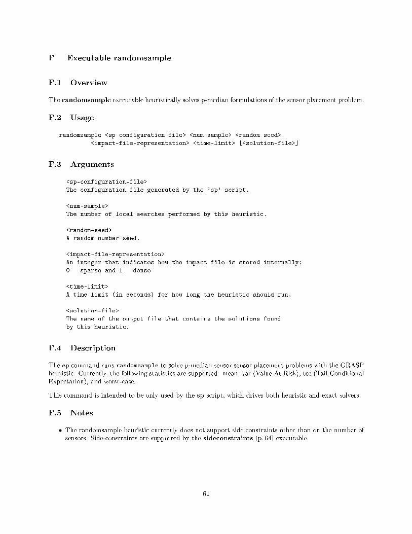
F Executable randomsample

F.1 Overview

The randomsample executable heuristically solves p-median formulations of the sensor placement problem.

F.2 Usage

randomsample <sp-configuration-file> <num-sample> <random-seed>

<impact-file-representation> <time-limit> [<solution-file>]

F.3 Arguments

<sp-configuration-file>

The configuration file generated by the 'sp' script.

<num-sample>

The number of local searches performed by this heuristic.

<random-seed>

A random number seed.

<impact-file-representation>

An integer that indicates how the impact file is stored internally:

0 - sparse and 1 - dense

<time-limit>

A time limit (in seconds) for how long the heuristic should run.

<solution-file>

The name of the output file that contains the solutions found

by this heuristic.

F.4 Description

The sp command runs randomsample to solve p-median sensor sensor placement problems with the GRASPheuristic. Currently, the following statistics are supported: mean, var (Value At Risk), tce (Tail-ConditionalExpectation), and worst-case.

This command is intended to be only used by the sp script, which drives both heuristic and exact solvers.

F.5 Notes

• The randomsample heuristic currently does not support side constraints other than on the number ofsensors. Side-constraints are supported by the sideconstraints (p. 64) executable.

61

G Executable scenarioAggr

G.1 Overview

The scenarioAggr executable takes an IMPACT �le and produces an aggregated impact �le.

G.2 Usage

scenarioAggr --numEvents=<num_incidents> <impact file>

G.3 Options

--numEvents=<number>

The number of incidents that should be aggregated.

G.4 Description

The scenarioAggr executable reads an IMPACT �le, �nds similar incidents, combines them, and writesout another IMPACT �le. The convention is to append the string "aggr" to the output.

The following �les are generated during the execution of scenarioAggr, assuming that the input was named"network.impact":

• aggrnetwork.impact - the new Impact File (p. 40)

• aggrnetwork.impact.prob - the probabilities of the aggregated incidents. These are non-uniform, soany solver must recognize incident probabilities.

G.5 Notes

• Not all solvers in SPOT can perform optimization with aggregated IMPACT �les. In particular,the heuristic GRASP solver does not currently support aggregation because it does not use incidentprobabilities. The Lagrangian and PICO solvers support incident aggregation. However, initial resultssuggest that although the number of incidents is reduced signi�cantly, the number of impacts may notbe, and solvers may not run much faster.

62

H Executable createIPData

H.1 Overview

The createIPData executable is used by the sp solver interface to setup an integer programming formulationfor sensor placement.

H.2 Command-Line Help

Usage : createIPData [ opt ions . . . ] <con f i g− f i l e >A command to generate AMPL data f i l e s , which are used by i n t e g e r programmings o l v e r s .

opt i ons :

−−gamma The f r a c t i o n o f the t a i l used to compute VaR andTCE s t a t i s t i c s

−h , −−help Display usage in fo rmat ion−−output The output f i l e−−ve r s i on Display ve r s i on in fo rmat ion

arguments :

con f i g− f i l e : Contains a l l o f the in fo rmat ion needed to setup a senso rplacement problem .

The createIPData executab l e i s used to setup an i n t e g e r programming problemfors enso r placement that can be so lved us ing the GeneralSP IP model . Thec on f i g u r a t i on f i l e input f i l e i s generated by the sp op t im i z a t i o n s c r i p t . Theoutput o f t h i s executab l e c o n s i s t s o f AMPL data commandsthat are used togenerate an in s t ance o f the GeneralSP IP model .

H.3 Description

The input �le used by createIPData is a Sensor Placement Con�guration File (p. 41). The output ofthis executable is sent to standard out, and it is in a format that can be processed by PICO (p. 60) and theAMPL solver interface.

H.4 Notes

• This executable is not meant to be run interactively.

• The scalability of this solver has not been well-characterized for large datasets, even when using ag-gressive aggregation.

63

I Executable sideconstraints

I.1 Overview

The sideconstraints executable heuristically solves p-median formulations of the sensor placement problemwhere one or more side-constraints are speci�ed. These side constraints are tight, meaning that any solutionthat violates the side constraints is considered infeasible.

I.2 Usage

sideconstraints <sp-configuration-file> <num-samples> <random-seed>

<impact-file-representation> <time-limit> [<solution-file>]

I.3 Arguments


The configuration file generated by the `sp' script.

<num-sample>

The number of local searches performed by this heuristic.

<random-seed>

A random number seed.

<impact-file-representation>

An integer that indicates how the impact file is stored internally:

0 - sparse and 1 - dense

<time-limit>

A time limit (in seconds) for how long the heuristic should run.

<solution-file>

The name of the output file that contains the solutions found

by this heuristic.

I.4 Description

The sp command runs sideconstraints to solve p-median sensor placement problems that include side-constraints with the GRASP heuristic. Currently, the following statistics are supported: mean, var (ValueAt Risk), tce (Tail-Conditional Expectation), and worst-case.

64

J Executable sp

J.1 Overview

The sp executable provides a common interface for sensor placement solvers in TEVA-SPOT.

J.2 Command-Line Help

Usage : sp [ opt ions ]

Options :−h , −−help show th i s he lp message and ex i t−n NETWORK, −−network=NETWORK

Name o f network f i l e−−ob j e c t i v e=OBJECTIVE

Object ive names have the form : <goal>_<s t a t i s t i c >. . The ob j e c t i v e goa l s are :. . . . c o s t the co s t o f s enso r placement. . . . ec extent o f contamination. . . . dec detec ted extent o f contamination. . . . td time to de t e c t i on. . . . dtd detec ted time to de t e c t i on. . . . mc mass consumed. . . . dmc detec ted mass consumed. . . . nfd number o f f a i l e d d e t e c t i on s. . . . ns the number o f s en s o r s. . . . pe populat ion exposed. . . . dpe detec ted populat ion exposed. . . . pk populat ion k i l l e d. . . . dpk detec ted populat ion k i l l e d. . . . pd populat ion dosed. . . . dpd detec ted populat ion dosed. . . . vc volume consumed. . . . dvc detec ted volume consumed. . The ob j e c t i v e s t a t i s t i c s are :. . . . mean the mean impact. . . . median the median impact. . . . var value−at−r i s k o f impact d i s t r i b u t i o n. . . . t c e t a i l−cond i t i oned expec ta t i on o f imp d i s t. . . . cvar approximation to TCE used with IPs. . . . worst the worst impactAn ob j e c t i v e name o f the form <goal> i s assumed tor e f e r to the ob j e c t i v e <goal>_mean . This opt ion maybe l i s t e d more than once .

−r DELAY, −−responseTime=DELAYThis parameter i n d i c a t e s the number o f minutes thatare needed to respond to the de t e c t i on o f acontaminant . As the response time in c r e a s e s , theimpact i n c r e a s e s because the contaminant a f f e c t s thenetwork f o r a g r e a t e r l ength o f time . Unit : minutes .

−g GAMMA, −−gamma=GAMMASp e c i f i e s the f r a c t i o n o f the d i s t r i b u t i o n o f impactsthat w i l l be used to compute the var , cvar and tcemeasures . Gamma i s assumed to l i e in the i n t e r v a l( 0 , 1 ] . I t can be i n t e r p r e t ed as s p e c i f y i n g the100∗gamma percent o f the worst contaminat ion i n c i d en t sthat are used f o r the se c a l c u l a t i o n s . Defau l t : . 05

−−i n c ident−weights=INCIDENT_WEIGHTSThis parameter s p e c i f i e s a f i l e that conta in s theweights f o r contamination i n c i d en t s . This f i l esupports the opt imiza t i on o f weighted impact metr i c s .By de fau l t , i n c i d en t s are opt imized with weight 1 .0

65

−−imper fect− s c f i l e=SCFILESp e c i f i e s the name o f a f i l e d e f i n i n g de t e c t i onp r o b a b i l i t i e s f o r a l l s enso r c a t e g o r i e s . Used with theimper fect−s enso r model . Must be s p e c i f i e d incon junct ion with the −−imper fect− j c f i l e opt ion .

−−imper fect− j c f i l e=JCFILESp e c i f i e s the name o f a f i l e d e f i n i n g a senso rcategory f o r each network junc t i on . Used with theimper fect−s enso r model . Must be s p e c i f i e d incon junct ion with the −−imper fect− s c f i l e opt ion .

−−num=NUMSAMPLES, −−numsamples=NUMSAMPLESSp e c i f i e s the number o f candidate s o l u t i o n s generatedby the grasp h e u r i s t i c . De fau l t s vary based ons t a t i s t i c and senso r model fo rmulat ion ( p e r f e c t vs .imper f e c t ) .

−−grasp−r ep r e s en t a t i on=GRASP_REPRESENTATIONSp e c i f i e s whether the grasp h e u r i s t i c uses a spar s ematrix (0 ) or dense matrix (1 ) r ep r e s en t a t i on to s t o r ethe impact f i l e contents . The d e f au l t i s 1 .

−−impact−d i r=IMPACT_DIRECTORYSp e c i f i e s the d i r e c t o r y the conta in s impact f i l e s . Byde f au l t the cur rent d i r e c t o r y i s used .

−−aggregat ion−th r e sho ld=AGGREGATION_THRESHOLD, −−th r e sho ld=AGGREGATION_THRESHOLDSp e c i f i e s the value ( as `<goal >,<value > ') used toaggregate ` s im i l a r ' impacts . This i s used to reducethe t o t a l s i z e o f the s enso r placement fo rmulat ion( f o r l a r g e problems ) . The s o l u t i o n generated with non−zero th r e sho ld s i s not guaranteed to be g l o b a l l yoptimal .

−−aggregat ion−percent=AGGREGATION_PERCENT, −−percent=AGGREGATION_PERCENTA `<goal >,<value >' pa i r where va lue i s a doublebetween 0 .0 and 1 . 0 . This i s an a l t e r n a t e way tocompute the aggregat ion th r e sho ld . Over a l lcontaminat ion in c id en t s , we compute the maximumd i f f e r e n c e d between the impact o f the contaminationi n c i d en t i s not detec ted and the impact i t i s detec tedat the e a r l i e s t p o s s i b l e f e a s i b l e l o c a t i o n . We s e tthe th r e sho ld to d ∗ aggregat ion_percent . I f bothth r e sho ld and percent are s e t to va l i d va lue s in thecommand l i n e , percent takes p r i o r i t y .

−−aggregat ion−r a t i o=AGGREGATION_RATIOA `<goal >,<value >' pa i r where va lue i s a doublebetween 0 .0 and 1 . 0 .

−−conserve−memory=MAXIMUM_IMPACTSI f l o c a t i o n aggregat i on i s chosen , and the o r i g i n a limpact f i l e s are very la rge , you can choose to p roce s sthem in a memory conse rv ing mode . For example "−−conserve_memory=10000" r eque s t s that whi l e o r i g i n a limpact f i l e s are being proce s sed in to sma l l e raggregated f i l e s , no more than 10000 impacts should beread in to memory at any one time . Defau l t i s 10000impacts . Set to 0 to turn t h i s o f f .

−−d i s t i n gu i s h−de t e c t i on=DISTINGUISH_GOAL, −−no−event−c o l l a p s e=DISTINGUISH_GOALA goa l f o r which aggregat i on should not a l lowi n c i d en t s to become t r i v i a l . That i s , i f the th r e sho ldi s so l a r g e that a l l l o c a t i on s , i n c l ud ing the dummy,would form a s i n g l e supe r l o ca t i on , t h i s f o r c e s thedummy to be in a supe r l o c a t i on by i t s e l f . Thus thes enso r placement w i l l d i s t i n g u i s h between de t e c t i ngand not de t e c t i ng . This opt ion can be l i s t e d mul t ip l etimes , to s p e c i f y mu l t ip l e goa l s . Note : the ` detected 'impact measures ( e . g . dec , dvc ) are alwaysd i s t i n gu i s h ed .

−−d i sab l e−aggregat i on=DISABLE_AGGREGATIONDisab le aggregat i on f o r t h i s goal , even at va lue zero ,which would incur no e r r o r . Each wi tnes s i n c i d en tw i l l be in a separa t e supe r l o c a t i on . This opt ion canbe l i s t e d mul t ip l e times , to s p e c i f y mu l t ip l e goa l s .

66

You may l i s t the goa l ` a l l ' to s p e c i f y a l l g oa l s .−−ub−c on s t r a i n t=UB_CONSTRAINT, −−ub=UB_CONSTRAINT

This opt ion s p e c i f i e s a c on s t r a i n t (<ob j e c t i v e >,<ub−value >) on the maximal va lue o f an ob j e c t i v e type .This opt ion can be repeated mul t ip l e t imes withd i f f e r e n t o b j e c t i v e s .

−−base l i n e−c on s t r a i n t=BASELINE_CONSTRAINT, −−ba s e l i n e=BASELINE_CONSTRAINTBase l i ne c on s t r a i n t s are not cu r r en t l y supported .

−−reduct ion−c on s t r a i n t=REDUCTION_CONSTRAINT, −−r educt i on=REDUCTION_CONSTRAINTReduction c on s t r a i n t s are not cu r r en t l y supported .

−−c o s t s=COST_FILE, −−cos t s_ids=COST_FILEThis f i l e conta in s c o s t s f o r the i n s t a l l a t i o n o fs en s o r s throughout the d i s t r i b u t i o n network . Thisf i l e conta in s id / co s t pa i r s , and de f au l t c o s t s can bes p e c i f i e d with the id : __default__ .

−−cos t s−i n d i c e s=COST_INDEX_FILEThis f i l e conta in s c o s t s f o r the i n s t a l l a t i o n o fs en s o r s throughout the d i s t r i b u t i o n network . Thisf i l e conta in s index / co s t pa i r s , and de f au l t c o s t s canbe s p e c i f i e d with the index : −1.

−−sensor−l o c a t i o n s=LOCATIONS_FILEThis f i l e conta in s in fo rmat ion about whether networki d s are f e a s i b l e f o r s enso r placement , and whether as enso r placement i s f i x ed at a g iven l o c a t i o n .

−−s o l v e r=SOLVER This opt ion s p e c i f i e s the type o f s o l v e r that i s usedto f i nd senso r placement ( s ) . The f o l l ow i ng s o l v e rtypes are cu r r en t l y supported :. . att_grasp mu l t i s t a r t l o c a l s earch h e u r i s t i c (AT&T). . snl_grasp TEVA−SPOT l i c e n s e−f r e e grasp c lone. . l ag rang ian lag rang ian r e l a x a t i o n h e u r i s t i c s o l v e r. . p i co mixed−i n t e g e r programming s o l v e r (PICO). . g lpk mixed−i n t e g e r programming s o l v e r (GLPK). . picoamp MIP s o l v e r with AMPL. . cplexamp commercial MIP s o l v e rThe de f au l t s o l v e r i s snl_grasp .

−−so l ve r−opt ions=SOLVER_OPTIONSThis opt ion conta in s so lve r−s p e c i f i c opt ions f o rc o n t r o l l i n g the s enso r placement s o l v e r . The opt ionsare added to the s o l v e r command l i n e .

−−runtime=RUNTIME Terminate the s o l v e r a f t e r the s p e c i f i e d number o fwa l l c l o ck minutes have e lapsed . By de fau l t , no l im i ti s p laced on the runtime . Some s o l v e r s can prov idet h e i r bes t s o l u t i o n so f a r at the po int o fte rminat ion .

−−no t i f y=INTERVAL Some s o l v e r s can output pre l im inary s o l u t i o n s whi l ethey are running . This opt ion supp l i e s the i n t e r v a l inminutes at which candidate s o l u t i o n s should be pr in tedout .

−−compute−bound Only compute a bound on the value o f the optimals o l u t i o n .

−−memmon Summarize the maximum memory used by any o f theexecu tab l e s

−−memcheck=MEMCHECKTARGETThis opt ion i n d i c a t e s that va l g r i nd should run on oneor more execu tab l e s .. . a l l run on a l l exe cu tab l e s. . s o l v e r run on the s o l v e r executab l e. . createIPData run on createIPData. . preproces s Impacts run on preprocess Impacts. . e v a l s en s o r run on eva l s en s o r. . aggregateImpacts run on aggregateImpacts Outputw i l l be wr i t t en to memcheck . { name} .{ pid } .

−−tmp− f i l e=TMP_FILE Name o f temporary f i l e p r e f i x used in t h i scomputation . The d e f au l t name i s `<network−name> '.

−o OUTPUT_FILE, −−output=OUTPUT_FILEName o f the output f i l e that conta in s the senso rplacement . The d e f au l t name i s `<network−name>. sensor s ' .

67

−−summary=SUMMARY_FILEName o f the output f i l e that conta in s summaryin fo rmat ion about the s enso r placement .

−−format=FORMAT Format o f the summary in fo rmat ion−−pr int−l og Pr int the s o l v e r output−−path=PATH Add th i s path to the s e t o f paths searched f o r

execu tab l e s and IP models .−−amplcplexpath=AMPLCPLEXPATH

Look f o r ampl and cplexamp executab l e s in t h i sd i r e c t o r y . This d e f a u l t s to a ` blank ' path , whichimp l i e s that the user ' s system path i s used .

−−picopath=PICOPATH Look f o r the PICO executab l e in t h i s d i r e c t o r y . Thisd e f a u l t s to the path used f o r execu tab l e s s p e c i f i e dby . the −−path opt ion .

−−glpkpath=GLPKPATH Look f o r the GLPK executab l e in t h i s d i r e c t o r y . Thisd e f a u l t s to the path used f o r execu tab l e s s p e c i f i e d bythe −−path opt ion .

−−ampl=AMPL The name o f the ampl executab l e ( t h i s d e f a u l t s to` ampl ' ) .

−−ampldata=AMPLDATA An aux i l l a r y AMPL data f i l e . This opt ion i s used wheni n t e g r a t i n g aux i l l a r y in fo rmat ion in to the AMPL IPmodel .

−−amplmodel=AMPLMODELAn a l t e r n a t i v e AMPL model f i l e . This opt ion i s usedwhen apply ing a non−standard AMPL model f o r s o l v i n gsenso r placement with an IP .

−−seed=SEED The value o f a seed f o r the random number genera torused by the s o l v e r . This can be used to ensure ade t e rm in i s t i c , r epea tab l e output from the s o l v e r .Should be >= 1 .

−−eval−a l l This opt ion s p e c i f i e s that a l l impact f i l e s found w i l lbe used to eva luate the f i n a l s o l u t i o n ( s ) .

−−debug L i s t s t a tu s messages whi l e p r o c e s s i ng .−−gap=GAP TODO gap help s t r i n g .−−ve r s i on Pr int v e r s i on in fo rmat ion f o r the compiled execu tab l e s

used by t h i s command .

J.3 Description

The sp executable is a Python script that coordinates the execution of the SPOT sensor placement solvers.The sp options can �exibly specify the objective to be optimized, as well as constraints on performance/costgoals.

The sp script currently interfaces with integer programming (IP) solvers, GRASP heuristics, and a La-grangian heuristic. The IP formulation can be used to �nd globally optimal solutions, the GRASP heuristichas proven e�ective at �nding optimal solutions to a variety of large-scale applications, and the Lagrangianheuristic �nds a near-optimal selection while computing a con�dence bound.

The following �les are generated during the execution of sp:

• <tmp�le>.con�g - the Sensor Placement Con�guration File (p. 41)

• <tmp�le>.dat - an AMPL data �le (if using an IP solver)

• <tmp�le>.mod - an AMPL script (if using an IP solver)

• <tmp�le>.log - a log �le that captures the solver output

• <tmp�le>.sensors - a Sensor Placement File (p. 39) that contains the �nal solution

68

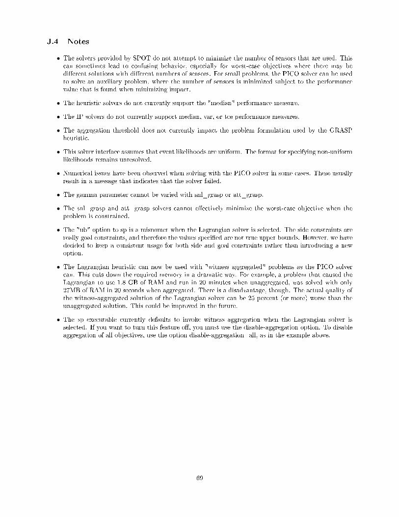
J.4 Notes

• The solvers provided by SPOT do not attempt to minimize the number of sensors that are used. Thiscan sometimes lead to confusing behavior, especially for worst-case objectives where there may bedi�erent solutions with di�erent numbers of sensors. For small problems, the PICO solver can be usedto solve an auxiliary problem, where the number of sensors is minimized subject to the performancevalue that is found when minimizing impact.

• The heuristic solvers do not currently support the "median" performance measure.

• The IP solvers do not currently support median, var, or tce performance measures.

• The aggregation threshold does not currently impact the problem formulation used by the GRASPheuristic.

• This solver interface assumes that event likelihoods are uniform. The format for specifying non-uniformlikelihoods remains unresolved.

• Numerical issues have been observed when solving with the PICO solver in some cases. These usuallyresult in a message that indicates that the solver failed.

• The gamma parameter cannot be varied with snl_grasp or att_grasp.

• The snl_grasp and att_grasp solvers cannot e�ectively minimize the worst-case objective when theproblem is constrained.

• The "ub" option to sp is a misnomer when the Lagrangian solver is selected. The side constraints arereally goal constraints, and therefore the values speci�ed are not true upper bounds. However, we havedecided to keep a consistent usage for both side and goal constraints rather than introducing a newoption.

• The Lagrangian heuristic can now be used with "witness aggregated" problems as the PICO solvercan. This cuts down the required memory in a dramatic way. For example, a problem that caused theLagrangian to use 1.8 GB of RAM and run in 20 minutes when unaggregated, was solved with only27MB of RAM in 20 seconds when aggregated. There is a disadvantage, though. The actual quality ofthe witness-aggregated solution of the Lagrangian solver can be 25 percent (or more) worse than theunaggregated solution. This could be improved in the future.

• The sp executable currently defaults to invoke witness aggregation when the Lagrangian solver isselected. If you want to turn this feature o�, you must use the disable-aggregation option. To disableaggregation of all objectives, use the option disable-aggregation=all, as in the example above.

69

K Executable sp-2tier

K.1 Overview

The sp-2tier executable provides a interface for sensor placement using a two-tiered approach in TEVA-SPOT. This executable calls the sp script. In tier 1, sp-2tier transforms the impact �le using geographicaggregation. The aggregated impact �le is used to �lter out candidate sensor placement locations. In tier 2,sp-2tier re�nes the original impact �le to include only candidate locations for the �nal sensor placement.sp-2tier uses spotSkeleton to de�ne the geographic proximity used to transform the original impact �le.See Section 5.9 (p. 29). for additional information on the two-tiered sensor placement approach.

K.2 Command-Line Help

Usage : sp_2t ier [ opt ions ]

Options :−h , −−help show th i s he lp message and ex i t−n NETWORK, −−network=NETWORK

Name o f network f i l e−−ob j e c t i v e=OBJECTIVE

Object ive names have the form : <goal>_<s t a t i s t i c >. . The ob j e c t i v e goa l s are :. . . . c o s t the co s t o f s enso r placement. . . . ec extent o f contamination. . . . dec detec ted extent o f contamination. . . . td time to de t e c t i on. . . . dtd detec ted time to de t e c t i on. . . . mc mass consumed. . . . dmc detec ted mass consumed. . . . nfd number o f f a i l e d d e t e c t i on s. . . . ns the number o f s en s o r s. . . . pe populat ion exposed. . . . dpe detec ted populat ion exposed. . . . pk populat ion k i l l e d. . . . dpk detec ted populat ion k i l l e d. . . . pd populat ion dosed. . . . dpd detec ted populat ion dosed. . . . vc volume consumed. . . . dvc detec ted volume consumed. . The ob j e c t i v e s t a t i s t i c s are :. . . . mean the mean impact. . . . median the median impact. . . . var value−at−r i s k o f impact d i s t r i b u t i o n. . . . t c e t a i l−cond i t i oned expec ta t i on o f imp d i s t. . . . cvar approximation to TCE used with IPs. . . . worst the worst impactAn ob j e c t i v e name o f the form <goal> i s assumed tor e f e r to the ob j e c t i v e <goal>_mean .

−−s k e l e t on=SKELETON Sp e c i f i e s the pipe diameter th r e sho ld used inspotSke l e ton .

−−s t a t=STAT S t a t i s t i c used in geographic aggregat ion o f the inputf i l e . Options in c lude :. . . min. . . max. . . mean. . . medianStreaming a lgor i thms are used to aggregate the impactf i l e . For the median option , the impact f i l e must beso r t ed .

−−ub1−c on s t r a i n t=UB1_CONSTRAINT, −−ub1=UB1_CONSTRAINT

70

This opt ion s p e c i f i e s a c on s t r a i n t (<ob j e c t i v e >,<ub−value >) on the maximal va lue o f an ob j e c t i v e type int i e r 1 .

−−ub2−c on s t r a i n t=UB2_CONSTRAINT, −−ub2=UB2_CONSTRAINTThis opt ion s p e c i f i e s a c on s t r a i n t (<ob j e c t i v e >,<ub−value >) on the maximal va lue o f an ob j e c t i v e type int i e r 2 .

−−s o l v e r 1=SOLVER1 This opt ion s p e c i f i e s the type o f s o l v e r that i s usedto f i nd senso r placement ( s ) in t i e r 1 . The f o l l ow i ngs o l v e r types are cu r r en t l y supported :. . att_grasp mu l t i s t a r t l o c a l s earch h e u r i s t i c (AT&T). . snl_grasp TEVA−SPOT l i c e n s e−f r e e grasp c lone. . l ag rang ian lag rang ian r e l a x a t i o n h e u r i s t i c s o l v e r. . p i co mixed−i n t e g e r programming s o l v e r (PICO). . g lpk mixed−i n t e g e r programming s o l v e r (GLPK). . picoamp MIP s o l v e r with AMPL. . cplexamp commercial MIP s o l v e rThe de f au l t s o l v e r i s snl_grasp .

−−s o l v e r 2=SOLVER2 This opt ion s p e c i f i e s the type o f s o l v e r that i s usedto f i nd senso r placment ( s ) in t i e r 2 . The f o l l ow i n gs o l v e r types are cu r r en t l y supported :. . att_grasp mu l t i s t a r t l o c a l s earch h e u r i s t i c (AT&T). . snl_grasp TEVA−SPOT l i c e n s e−f r e e grasp c lone. . l ag rang ian lag rang ian r e l a x a t i o n h e u r i s t i c s o l v e r. . p i co mixed−i n t e g e r programming s o l v e r (PICO). . g lpk mixed−i n t e g e r programming s o l v e r (GLPK). . picoamp MIP s o l v e r with AMPL. . cplexamp commercial MIP s o l v e rThe de f au l t s o l v e r i s snl_grasp .

−−path=PATH Add th i s path to the s e t o f paths searched f o rexecu tab l e s and IP models .

K.3 Description

Based on the command line naming conventions, the following �les are required for execution of sp-2tier:

INPUT FILE DESCRIPTIONNETWORK.inp Original EPANET input �leNETWORK_OBJECTIVE.impact Impact �le for a single objective, output from tevasim/tso2impact using the

original EPANET input �le.NETWORK.nodemap Nodemap �le used to translate between epanetID (used in the inp �le) and

nodeID (used in the impact �le).

From the data directory, sp-2tier creates a results directory called NETWORK_SKELETON. For example, Net3_8contains output �les from sp-2tier using Net3 and a skeleton threshold of 8 inches. The following �les aregenerated during the execution of sp-2tier:

71

OUTPUT FILE DESCRIPTIONNETWORK_SKELETON.inp Skeletonized EPANET inp �leNETWORK_SKELETON.map Map �le (notation in epanetID)SKELETON_time.out Time used to run spotSkeletonSKELETON_memmon.out Memory used to run spotSkeletonNETWORK_SKELETON_OBJECTIVE.impact Impact �le after geographic aggregationNETWORK_SKELETON.nodemap Nodemap �le after geographic aggregationaggregate_time.out Time used to aggregate the impact �leaggregate_memmon.out Memory used to aggregate the impact �leNETWORK_SKELETON.log sp log �le for tier 1 sensor placementNETWORK_SKELETON.sensors sp sensors �le for tier 1 sensor placementNETWORK_SKELETON.con�g sp con�g �le for tier 1 sensor placementsp1_SKELETON.out sp output �le for tier 1 sensor placement. Contains memory used.sp1_time.out Time used to run tier 1 sensor placementNETWORK_SKELETONR_OBJECTIVE.impact Re�ned impact �le based on sp1 resultNETWORK_SKELETONR.nodemap Re�ned nodemap �le. This �le contains 4 columns (as opposed to the stan-

dard 2 for nodemap �les) and is used to convert between re�ned nodeID andepanetID on the original network. Col1 = nodeID in the re�ned impact �le.Col2 = supernode membership. Col3 = nodeID in the original impact �le.Col4 = epanetID in the original inp �le

re�ne_time.out Time used to re�ne the impact �lere�ne_memmon.out Memory used to re�ne the impact �leNETWORK_SKELETONR.log sp log �le for tier 2 sensor placementNETWORK_SKELETONR.sensors sp sensors �le for tier 2 sensor placementNETWORK_SKELETONR.con�g sp con�g �le for tier 2 sensor placementsp2_SKELETONR.out sp output �le for tier 2 sensor placement. Contains memory used.sp2_time.out Time used to run tier 2 sensor placement

K.4 Notes

• sp-2tier will not recreate the skeletonized inp and map �les if the �le NETWORK_SKELETON.map is inthe results directory NETWORK_SKELETON.

• sp-2tier will not recreate the aggregated impact �le if the �le NETWORK_SKELETON_OBJECTIVE.impactis in the results directory NETWORK_SKELETON.

72

L Executable spotSkeleton

L.1 Overview

The TEVA-SPOT skeletonizer, spotSkeleton, reduces the size of a network model by grouping neighbor-ing nodes based on the topology of the network and pipe diameter threshold. spotSkeleton requires anEPANET inp network �le and a pipe diameter threshold along with output �le names for the skeletonizedEPANET inp network �le and map �le. spotSkeleton contracts connected pieces of the network into asingle node; this node is call a supernode. The map �le de�nes the nodes that belong to each supernode.

L.2 Usage

spotSkeleton <input inp file> <pipe diameter threshold> <output inp file> <output map file>

L.3 Description

spotSkeleton includes branch trimming, series pipe merging, and parallel pipe merging. A pipe diameterthreshold determines candidate pipes for skeleton steps. spotSkeleton maintains pipes and nodes withhydraulic controls as it creates the skeletonized network. It performs series and parallel pipe merges if bothpipes are below the pipe diameter threshold, calculating hydraulic equivalency for each merge based onthe average pipe roughness of the joining pipes. For all merge steps, the larger diameter pipe is retained.For a series pipe merge, demands (and associated demand patterns) are redistributed to the nearest node.Branch trimming removes deadend pipes smaller than the pipe diameter threshold and redistributes demands(and associated demand patterns) to the remaining junction. spotSkeleton repeats these steps until nofurther pipes can be removed from the network. spotSkeleton creates an EPANET-compatible skeletonizednetwork inp �le and a 'map �le' that contains the mapping of original network model nodes into skeletonizedsupernodes.

Under the skeletonization steps described above, there is a limit to how much a network can be reducedbased on its topology, e.g., number of deadend pipes, or pipes in series and parallel. For example, sectionsof the network with a loop, or grid, structure will not reduce under these skeleton steps. Additionally, thenumber of hydraulic controls in�uences skeletonization, as all pipes and nodes associated with these featuresare preserved.

L.4 Notes

• Commercial skeletonization codes include Haestad Skelebrator, MWHSoft H2OMAP, and MWHSoftInfoWater. Two-tiered sensor placement requires mapping between the skeletonized and original net-work (map �le). Commercial skeletonizers do not provide this information directly. The MWHSoftInfowater/H2OMAP history log �le provides it indirectly in a history log �le. The history log �le trackssequential skeleton steps and records merge and trim operations on a pipe-by-pipe basis.

• To validate spotSkeleton, we compared its output to that of MWHSoft H2OMAP and Infowater.Input parameters were chosen to match spotSkeleton options. Pipe diameter thresholds of 8 inches, 12inches, and 16 inches were tested using two large networks. MWHSoft and TEVA-SPOT skeletonizerswere compared using the Jaccard index (Jaccard, 1901). The Jaccard index measures similarity betweentwo sets by dividing the intersection of the two sets by the union of the two sets. In this case, theintersection is the number of pipes that are either both removed or not removed by the two skeletonizers,the union is the number of all pipes in the original network. If the two skeletonizers de�ne the samesupernodes, the Jaccard index equals 1. Skeletonized networks from the MWHSoft and TEVA-SPOT

73

skeletonizers result in a Jaccard index between 0.93 and 0.95. Thus, we believe the spotSkeleton isa good substitute for commercial skeletonizers.

74

M Executable tevasim

M.1 Overview

The tevasim executable uses EPANET to perform an ensemble of contaminant transport simulations.

M.2 Command-Line Help

Usage : tevasim [ opt ions ] <epanet−input− f i l e > <epanet−output− f i l e ><erd−db−name>

A u t i l i t y f o r running an ensemble o f water qua l i t y s imulat ions , whose r e s u l t sare s to r ed in a TSO f i l e .

opt i ons :

−−dvf The Dec i s i on Var iab le F i l e (DVF) f i l e used tos p e c i f y the f l u s h i n g / va lve c on t r o l s .

−h , −−help Display usage in fo rmat ion−−mss The MSX sp e c i e s to save .−−msx The MSX f i l e f o r s p e c i f y i n g multi−s p e c i e s

EPANET.−−t sg The TSG f i l e used to s p e c i f y the i n j e c t i o n

i n c i d en t s .−−t s i The TSI f i l e used to s p e c i f y the i n j e c t i o n

i n c i d en t s .−−ve r s i on Display ve r s i on in fo rmat ion

arguments :

epanet−input− f i l e : EPANET network f i l e .

epanet−output− f i l e : Output f i l e generated by EPANET.

erd−db−name : The ERD database name . A d i r e c t o r y can be s p e c i f i e d as parto f t h i s name − i f the r e i s one , the db f i l e s w i l l be s to r ed there

The tevasim command i s used to s imulate contaminat ion i n c i d en t s . This commanduses EPANET to perform an ensemble o f contaminant t ranspo r t s imulat ions ,de f i ned by a TSG F i l e . The f o l l ow i ng f i l e s are generated during the execut iono f tevasim :− a binary ERD f i l e that conta in s the contaminat ion t ranspor t data ,− a binary SDX f i l e that prov ide s an index in to the ERD Fi l e , and− an output f i l e that prov ide s a t ex tua l summary o f the EPANET s imu la t i on s .

Note that opt ions l i k e ` tsg ' can be s p e c i f i e d with the syntax `−− t sg f i l e . tsg 'or `−− t sg=f i l e . tsg ' .

75

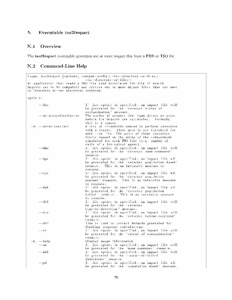
N Executable tso2Impact

N.1 Overview

The tso2Impact executable generates one or more impact �les from a ERD or TSO �le.

N.2 Command-Line Help

Usage : tso2Impact [ opt ions ] <output−pre f i x > <tso−d i r e c to ry−or− f i l e s ><ta i−d i r e c to ry−or− f i l e s >

An app l i c a t i on that reads a TSO f i l e ( and a s s o c i a t ed TAI f i l e i f hea l thimpacts are to be computed ) and c r e a t e s one or more impact f i l e s that are usedto formulate s enso r placement problems .

opt ions :

−−dec I f t h i s opt ion i s s p e c i f i e d , an impact f i l e w i l lbe generated f o r the ` detec ted extent o fcontamination ' measure .

−−detec t i onConf idence The number o f s en s o r s that must de t e c t an eventbe f o r e the impacts are c a l c u l a t ed . Normallyt h i s i s 1 s enso r .

−d , −−de te c t i onL imi t A l i s t o f th r e sho ld s needed to perform de t e c t i onwith a senso r . There must be one th r e sho ld f o reach . t so f i l e . The un i t s o f the se de t e c t i onl im i t s depend on the un i t s o f the contaminants imulated f o r each TSO f i l e ( e . g . number o fc e l l s o f a b i o l o g i c a l agent ) .

−−dmc I f t h i s opt ion i s s p e c i f i e d , an impact f i l e w i l lbe generated f o r the ` detec ted mass consumed 'measure .

−−dpd I f t h i s opt ion i s s p e c i f i e d , an impact f i l e w l lbe generated f o r the ` detec ted populat ion dosed 'measure . This i s an i n t e n s i v e measure tocompute .

−−dpe I f t h i s opt ion i s s p e c i f i e d , an impact f i l e w l lbe generated f o r the ` detec ted populat ionexposed ' measure . This i s an i n t e n s i v e measureto compute .

−−dpk I f t h i s opt ion i s s p e c i f i e d , an impact f i l e w l lbe generated f o r the ` detec ted populat ionk i l l e d ' measure . This i s an i n t e n s i v e measureto compute .

−−dtd I f t h i s opt ion i s s p e c i f i e d , an impact f i l e w i l lbe generated f o r the ` detec tedtime−to−detec t ion ' measure .

−−dvc I f t h i s opt ion i s s p e c i f i e d , an impact f i l e w i l lbe generated f o r the ` detec ted volume consumed 'measure .

−−dvf This i s used to c o r r e c t demands generated f o rf l u s h i n g response c a l c u l a t i o n s

−−ec I f t h i s opt ion i s s p e c i f i e d , an impact f i l e w i l lbe generated f o r the ` extent o f contamination 'measure .

−h , −−help Display usage in fo rmat ion−−mc I f t h i s opt ion i s s p e c i f i e d , an impact f i l e w i l l

be generated f o r the `mass consumed ' measure .−−nfd I f t h i s opt ion i s s p e c i f i e d , an impact f i l e w i l l

be generated f o r the ` number−of−f a i l e dde t e c t i on s ' measure .

−−pd I f t h i s opt ion i s s p e c i f i e d , an impact f i l e w l lbe generated f o r the ` populat ion dosed ' measure .

76

This i s an i n t e n s i v e measure to compute .−−pe I f t h i s opt ion i s s p e c i f i e d , an impact f i l e w l l

be generated f o r the ` populat ion exposed 'measure . This i s an i n t e n s i v e measure tocompute .

−−pk I f t h i s opt ion i s s p e c i f i e d , an impact f i l e w l lbe generated f o r the ` populat ion k i l l e d 'measure . This i s an i n t e n s i v e measure tocompute .

−r , −−responseTime This opt ion i n d i c a t e s the number o f minutes thatare needed to respond to the de t e c t i on o f acont inant . As the response time in c r e a s e s , theimpact i n c r e a s e s because the contaminant a f f e c t sthe network f o r a g r e a t e r l ength o f time . Unit :minutes .

−−s p e c i e s Name o f s p e c i e s to use in computing impacts .−−td I f t h i s opt ion i s s p e c i f i e d , an impact f i l e w i l l

be generated f o r the ` time−to−detec t ion 'measure .

−−t e c I f t h i s opt ion i s s p e c i f i e d , an impact f i l e w i l lbe generated f o r the ` timed extent o fcontamination ' measure .

−−vc I f t h i s opt ion i s s p e c i f i e d , an impact f i l e w i l lbe generated f o r the ` volume consumed ' measure .

−−ve r s i on Display ve r s i on in fo rmat ion

arguments :

output−p r e f i x : The p r e f i x used f o r a l l f i l e s generated by tso2Impact .

erd−or−tso− f i l e : This argument i n d i c a t e s e i t h e r a TSO or ERD f i l e .

ta i−d i r e c to ry−or− f i l e : This argument i n d i c a t e s a TAI f i l e name . The TAIinput f i l e i s a th rea t_as se s s input that s p e c i f i e s parameters l i k edosage , response , l e t h a l i t y , e t c . There should be one TAI f i l e f o r eachTSO f i l e .

Note that opt ions l i k e ` responseTime ' can be s p e c i f i e d with the syntax`−−responseTime 10 . 0 ' or `−−responseTime =10.0 ' .

N.3 Description

The tso2Impact executable generates impact �les that are used for sensor placement. This executableprocesses a ERD or TSO File (p. 39), which summarizes the result of an EPANET computation. Thefollowing �les are generated during the execution of tso2Impact:

• <output-pre�x>.nodemap - a Node File (p. 41).

• <output-pre�x>.scenariomap - a Scenario File (p. 41).

• <output-pre�x>_<impact-type>.impact - an Impact File (p. 40) for a given impact.

N.4 Notes

• The `--tsoPattern` option allows a set of ERD or TSO �les to be speci�ed without explicitly listing allof them on the command-line. The user speci�es a regular expression, and all �les that match thatexpression are included in the analysis.

77

O Executable u�

O.1 Overview

The u� executable heuristically solves p-median formulations of the sensor placement problem while alsocomputing a valid lower bound on the best possible sensor placement value.

O.2 Usage

ufl <sp-configuration-file> <p> [--gap=<fraction>][<goal-constraint-data-file> <upper-bound>]

O.3 Options

--gap=<fraction>

This option tells the solver to stop when the solution is within a certain percentage

of optimal. Let \b icost be the current best integer solution found and \b lb be the

current lower bound. The solver will stop with <b> (icost - lb)/lb </b> is less that

the gap. For example, if the gap is 0.1, then the solver will stop when it has a

solution that is within 10 percent of optimality.

O.4 Arguments


A LAG file that defines impacts for the objective.

<p>

The number of sensors.

<goal-constraint-data-file>

A LAG file that defines impacts for a side-constraint.

<upper-bound>

The upper bound for this side constraint.

O.5 Description

"u�" stands for "uncapacitated facility location," and this code is a Sandia-modi�ed version of the com-bination of Lagrangian relaxation and the "Volume Algorithm" that is found in the open-source "COIN"repository (that the PICO solver uses).

The sp executable automatically generates u� commands, including those with goal constraints. The userspeci�es the number of sensors, and sp passes to u� one more than this number. The Lagrangian heuristicimplemented in u� then places the correct number of sensors, and one "dummy" sensor that catches allundetected events.

Note that the u� command uses LAG File (p. 40) inputs, which are a modi�ed format of impact �les.These �les are generated by the tso2Impact (p. 76) executable.

As of teva-spot-1.2, u� handles "goal constraints." For example, we may minimize the contaminant massconsumed subject to the goal of limiting the extent of contamination in pipe feet to a constant such as

78

15,000. This is di�erent from specifying a side constraint for the "sideconstraints" local search executable.The latter will reject any solution in which the extent of contamination is greater than 15,000, even if it isonly 15,001. Many goal constraints may be provided simultaneously, and the Lagrangian solver will attemptto �nd a solution that honors those constraints. It will report one that has a good combination of primaryobjective value and small violations of the goals.

This technology is young, and experience shows that user attempts to make the goal constraints too tight canconfuse the solver. We o�er the following guidance to avoid this problem. Suppose that we wish to use theLagrangian heuristic to �nd a good solution that minimizes the average contaminant mass consumed subjectto utility guidelines on the average extent of contamination, and also the average volume of contaminatedwater consumed.

1. Using a solver of choice for the particular problem, �nd single-objective optimal values for each objec-tive.

2. Using evalsensor, evaluate the single-objective sensor placements against each of the other objectives.The result is a matrix of objective values.

3. Determine goal constraints for the secondary objectives by selecting a value between the optimalsingle-objective value for that secondary objective, and its value under the sensor placement obtainedby solving the single-objective problem for the primary objective.

For example, for a real test problem, minimizing the average contaminant mass consumed yielded an objectivevalue of 638,344 units. Taking the sensor placement obtained from that solve, we found that the averageextent of contamination was 78,037 feet, and the average volume of contaminated water consumed was282,689 units.

Solving individually for these objectives, we found that the optimal solutions for extent of contaminationand volume consumed were 40,867 and 217,001, respectively. From this information, we decided to applygoal constraints of 45,000 feet for the extent of contamination, and 250,000 units for the volume consumed.

Minimizing the mass consumed with these two goal constraints, the Lagrangian heuristic found a new sensorplacement that incurred objective values of 678,175 units for mass consumed, 49,016 feet for the extent ofcontamination, and 256,615 units for volume consumed. Note that neither goal was strictly met, but eachgoal helped improve its related objective value.

We now compare this technology to the side-constrained local search heuristic (the "sideconstraints" exe-cutable). Each heuristic has advantages and disadvantages. The goal-constrained Lagrangian solver canhandle an arbitrary number of goal constraints, producing a solution that is well balanced, as above. Whenwe attempt to reproduce the results above using the "sideconstraints" executable, which is currently limitedto only one side constraint, we see the untreated objective su�er. For example, with the same setup asabove, and a side constraint of 50,000 feet for average extent of contamination, the sideconstraints heuristicproduces a solution with an expected mass consumed of 670,399 units, an expected extent of contaminationof 49,827 feet, and an expected volume consumed of 326,943. We see a similar type of result with a singleside constraint on the volume consumed (the extent of contamination increases substantially). The sidecon-straints code could be extended to handle multiple side constraints, of course, but the neighborhood searchmight have di�culty �nding feasible solutions. Since Lagrangian relaxation is a global technique and slightlyinfeasible solutions are permitted, we are more likely to �nd a good trade-o�.

However, the Lagrangian heuristic has disadvantages as well. If a particular goal constraint is set too tightly,the solution can degenerate such that all of the objectives get substantially worse. We do not understand thisphenomenon well yet, and further research into the algorithm itself may be necessary to make this technologygenerally usable. For now, it is sometimes necessary to manipulate the values of the goal constraints manuallyin order to �nd a good solution.

79

SCIENCE

EPA 600/R-08/041B | September 2012 | www.epa.gov/ord

United StatesEnvironmental ProtectionAgency

Office of Research and DevelopmentNational Homeland Security Research CenterCincinnati, OH 45268

Official BusinessPenalty for Private Use$300

PRESORTED STANDARDPOSTAGE & FEES PAID

EPAPERMIT NO. G-35

Documents

Unit ed Sta te s E n v ironment al P rot ect ion IE NSC