Embed Size (px)
Citation preview
UNIT I ISDN – STANDARDS AND SERVICES
Switching networks•Long distance transmission are done over anetwork of switched nodes. Nodes notconcerned with content of data.•End devices are stations:Computer, terminal, phone,etc.•A collection of nodes and connection is anetwork.•Data routed being by network node by node.
Switching networks•Long distance transmission are done over anetwork of switched nodes. Nodes notconcerned with content of data.•End devices are stationsComputer,terminal,phone,etc.•A collection of nodes and connection is anetwork.•Data routed being by network node by node.
Nodes:•Nodes may connect to other nodes only, or to stations and other nodes•Node to node links usually multiplexed•Network is usually partially connected
Some redundant connections are desirable for reliability
•Two different switching technologiesCircuit switchingPacket switching
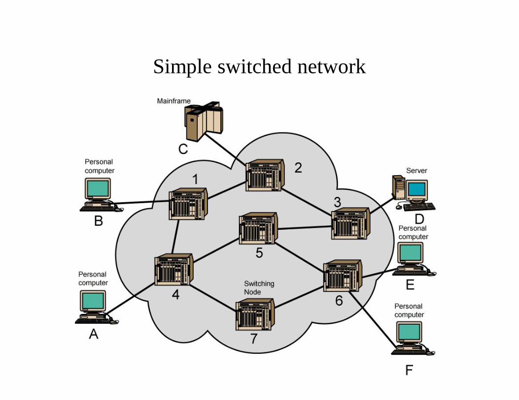
Simple switched network
Circuit switching
•Dedicated communication path betweentwo stations•Three phases
EstablishTransferDisconnect
•Must have switching capacity and channelcapacity to establish connection`•Must have intelligence to work out routing
Circuit Switching Concepts•Digital Switch
Provide transparent signal pathbetween devices
•Network Interface•Control Unit
Establish connectionsGenerally on demandHandle and acknowledgerequestsDetermine if destination is freeconstruct path
•Maintain connection•Disconnect
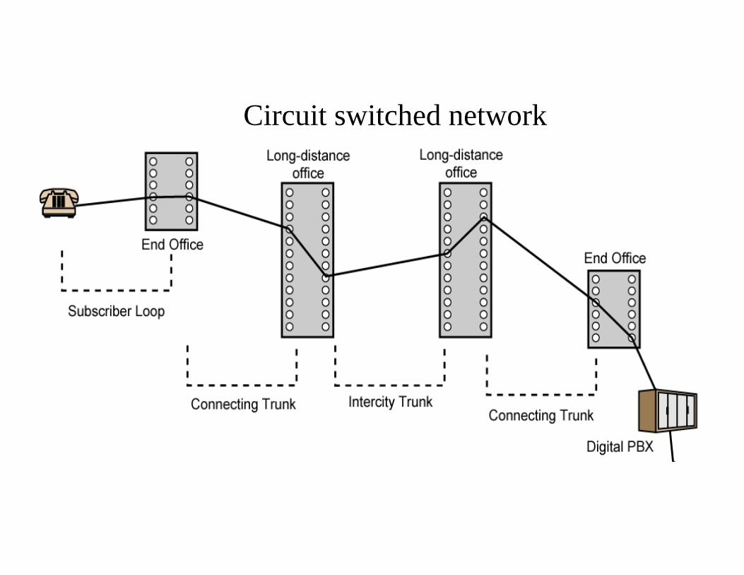
Circuit switched network
Telecomms Components
•SubscriberDevices attached to network
•Subscriber lineLocal LoopSubscriber loopConnection to networkFew km up to few tens of km
•ExchangeSwitching centersEnd office - supports subscribers
Packet Switching PrinciplesPacket switching designed for voice
•Resources dedicated to a particular call•Much of the time a data connection isidle•Data rate is fixed•Both ends must operate at the same rate
•Data transmitted in small packetsTypically 1000 octets•Longer messages split into seriesof packets•Each packet contains a portion ofuser data plus some control info
•Control info Routing (addressing)info Packets are received, storedbriefly (buffered) and past on to thenext node•Store and forward
Switching Techniques:
•Station breaks long message into packets•Packets sent one at a time to the network•Packets handled in two ways
DatagramVirtual circuit
Datagram:
•Each packet treated independently•Packets can take any practical route•Packets may arrive out of order•Packets may go missing•Up to receiver to re-order packets and recover from missing packets
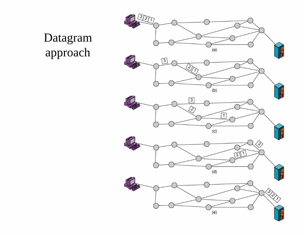
Datagram approach
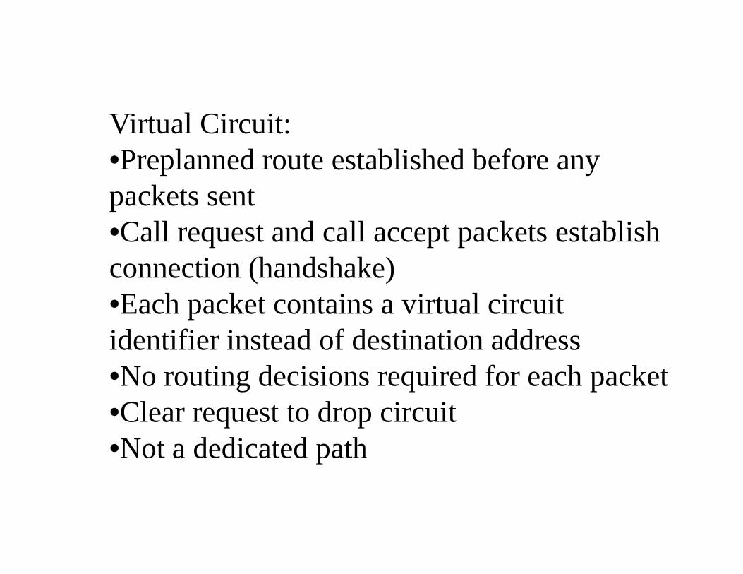
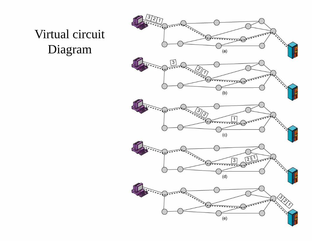
Virtual Circuit:•Preplanned route established before any packets sent•Call request and call accept packets establish connection (handshake)•Each packet contains a virtual circuit identifier instead of destination address•No routing decisions required for each packet•Clear request to drop circuit•Not a dedicated path
Virtual circuit Diagram
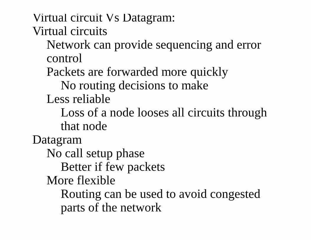
Virtual circuit Vs Datagram:Virtual circuits
Network can provide sequencing and error controlPackets are forwarded more quickly
No routing decisions to makeLess reliable
Loss of a node looses all circuits through that node
DatagramNo call setup phase
Better if few packetsMore flexible
Routing can be used to avoid congested parts of the network
Circuit Vs Packet switching:Performance
Propagation delayTransmission timeNode delay
The importance of switching in communication• The cost of switching is high
Definition: Transfer input sample points to the correct output ports at the correct time Terminology :
• Switching • Digital switching (sample points amplitudes are 0's and 1's) • PABX • Circuit • Circuit switching • Packet switching
Integrated Services Digital Network
• Public networks are used for a variety of services– Public Switched Telephone Network– Private Lines (leased)– Packet Switched Data Networks– Circuit Switched Data networks
ISDN
• Users have a variety of equipment to connect to public networks– Telephones– Private Branch Exchanges– Computer Terminals or PCs– Mainframe Computers
• A variety of physical interfaces and access procedures are required for connection
ISDN
• The telephone network has evolved into a digital one with digital exchanges and links
• The signalling system has become a digital message-oriented common channel signalling system (SS#7)
• The term ‘Integrated Digital Network’ is used to describe these developments
ISDN
• The Public Switched Telephone network is still analogue from the subscriber to the local exchange
• The need has arisen to extend the digital network out to subscribers and to provide a single standardised interface to all different users of public networks
• ISDN fulfils that need
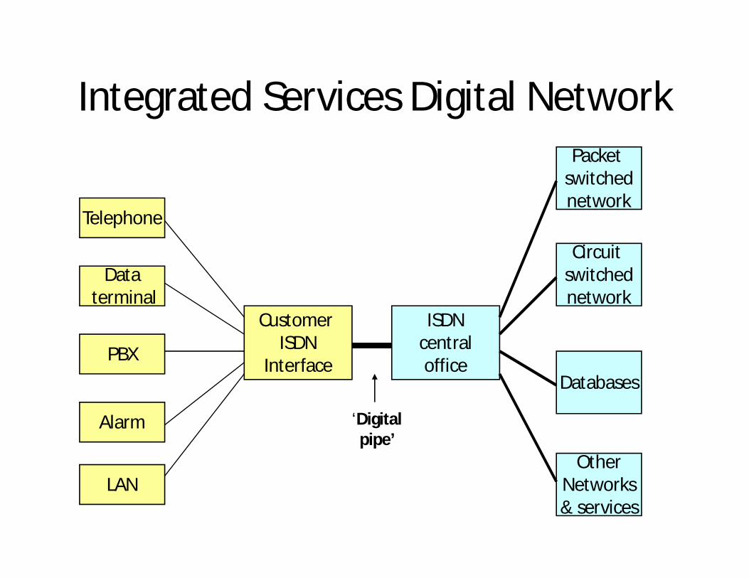
Integrated Services Digital Network
Telephone
Dataterminal
PBX
Alarm
LAN
Customer ISDN
Interface
ISDNcentraloffice
Packet switchednetwork
Circuit switchednetwork
Databases
OtherNetworks& services
‘Digitalpipe’
ISDN
• In Practice there are multiple networks providing the service nationally
• The user however, sees a single network

Benefits to Subscribers
• Single access line for all services• Ability to tailor service purchased to suit needs• Competition among equipment vendors due to
standards• Availability of competitive service providers
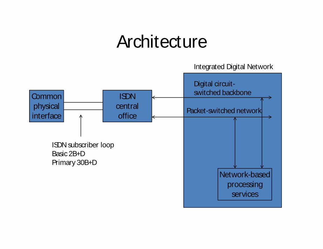
Architecture
Commonphysicalinterface
ISDNcentraloffice
Network-basedprocessing
services
Digital circuit-switched backbone
Packet-switched network
Integrated Digital Network
ISDN subscriber loopBasic 2B+DPrimary 30B+D
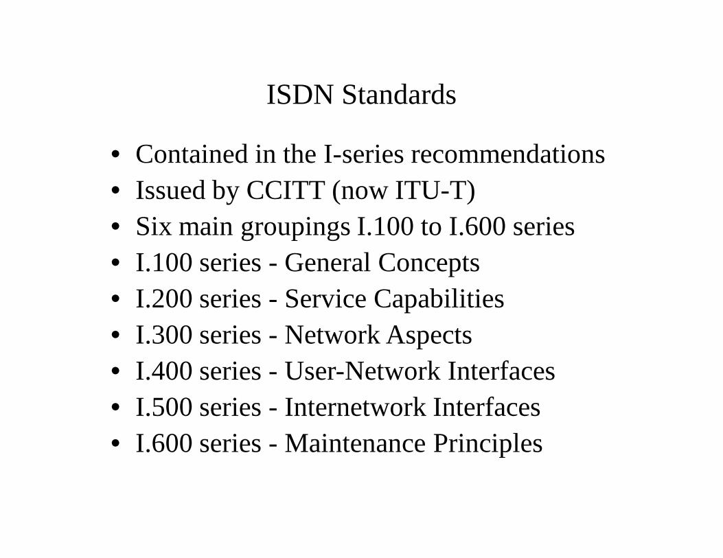
ISDN Standards
• Contained in the I-series recommendations• Issued by CCITT (now ITU-T)• Six main groupings I.100 to I.600 series• I.100 series - General Concepts• I.200 series - Service Capabilities• I.300 series - Network Aspects• I.400 series - User-Network Interfaces• I.500 series - Internetwork Interfaces• I.600 series - Maintenance Principles
ISDN Channels
• The Digital pipe is made up of channels - one of three types
• B channel, D channel or H channel• Channels are grouped and offered as a package
to users
B Channel
• B channel-64 kbps • B is basic user channel
– can carry digital data or PCM-encoded voice – or mixture of lower rate traffic.
B Channel
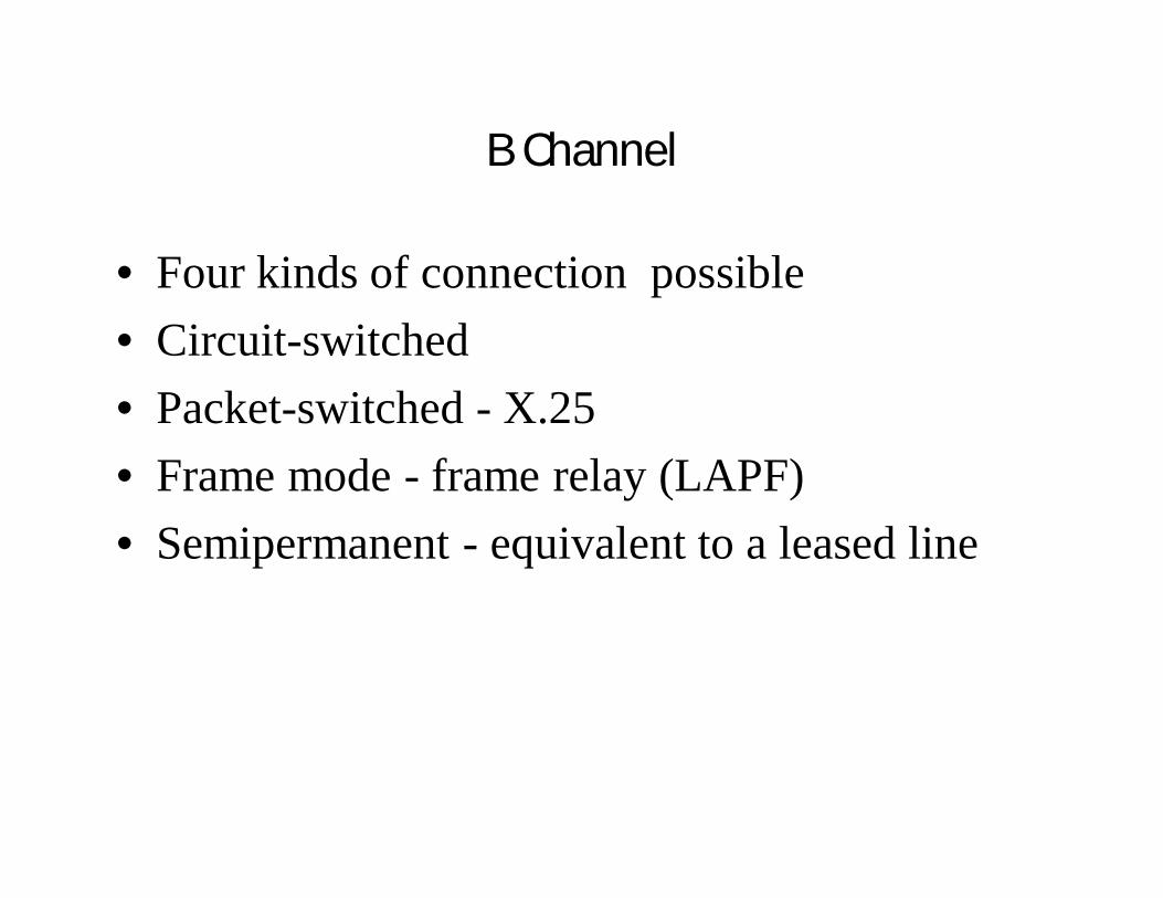
• Four kinds of connection possible• Circuit-switched• Packet-switched - X.25• Frame mode - frame relay (LAPF)• Semipermanent - equivalent to a leased line
D Channel
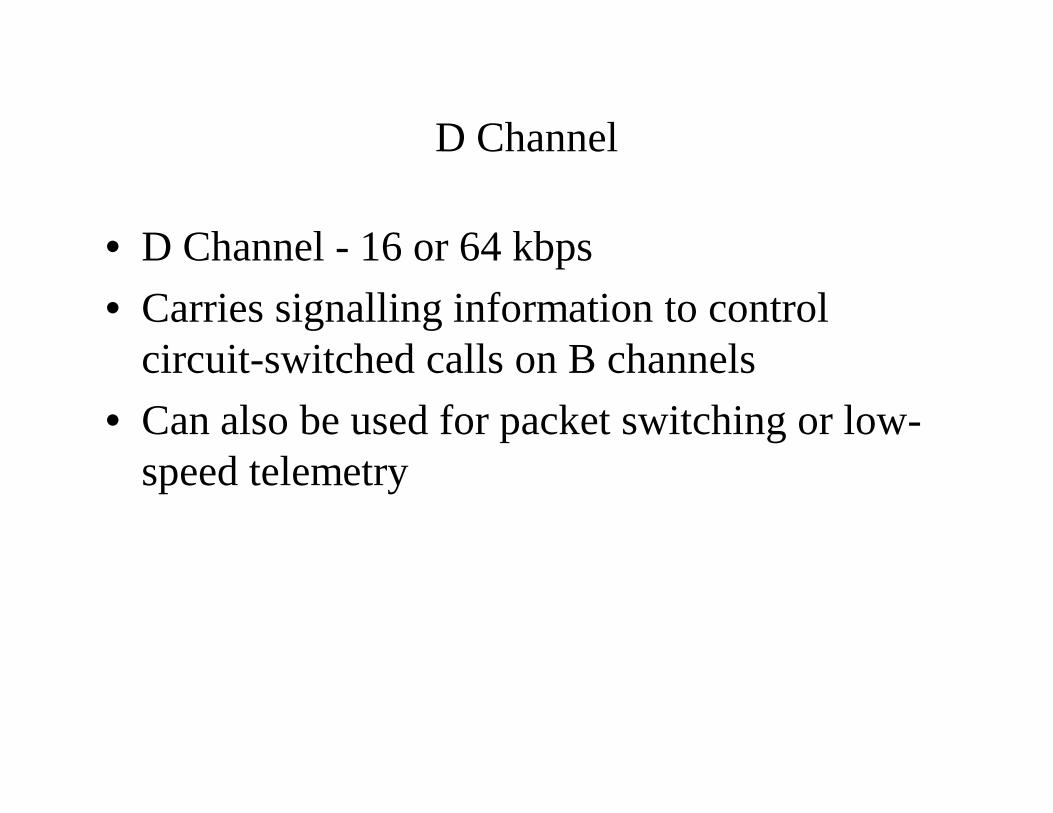
• D Channel - 16 or 64 kbps• Carries signalling information to control
circuit-switched calls on B channels• Can also be used for packet switching or low-
speed telemetry
H Channel
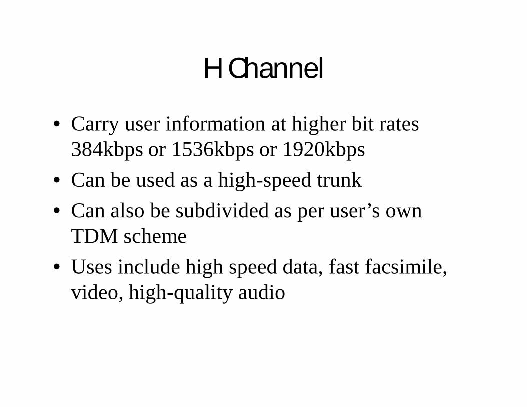
• Carry user information at higher bit rates 384kbps or 1536kbps or 1920kbps
• Can be used as a high-speed trunk• Can also be subdivided as per user’s own
TDM scheme• Uses include high speed data, fast facsimile,
video, high-quality audio
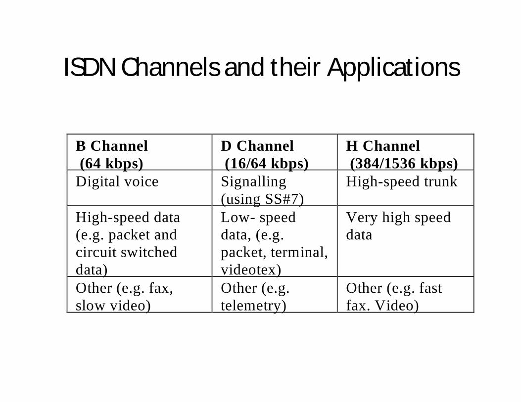
ISDN Channels and their Applications
B Channel (64 kbps)
D Channel (16/64 kbps)
H Channel (384/1536 kbps)
Digital voice Signalling(using SS#7)
High-speed trunk
High-speed data(e.g. packet andcircuit switcheddata)
Low- speeddata, (e.g.packet, terminal,videotex)
Very high speeddata
Other (e.g. fax,slow video)
Other (e.g.telemetry)
Other (e.g. fastfax. Video)
ISDN Channel Groupings
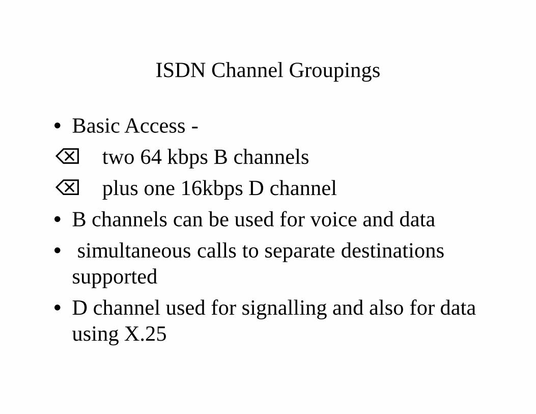
• Basic Access - two 64 kbps B channels plus one 16kbps D channel• B channels can be used for voice and data• simultaneous calls to separate destinations
supported• D channel used for signalling and also for data
using X.25
ISDN Basic Access
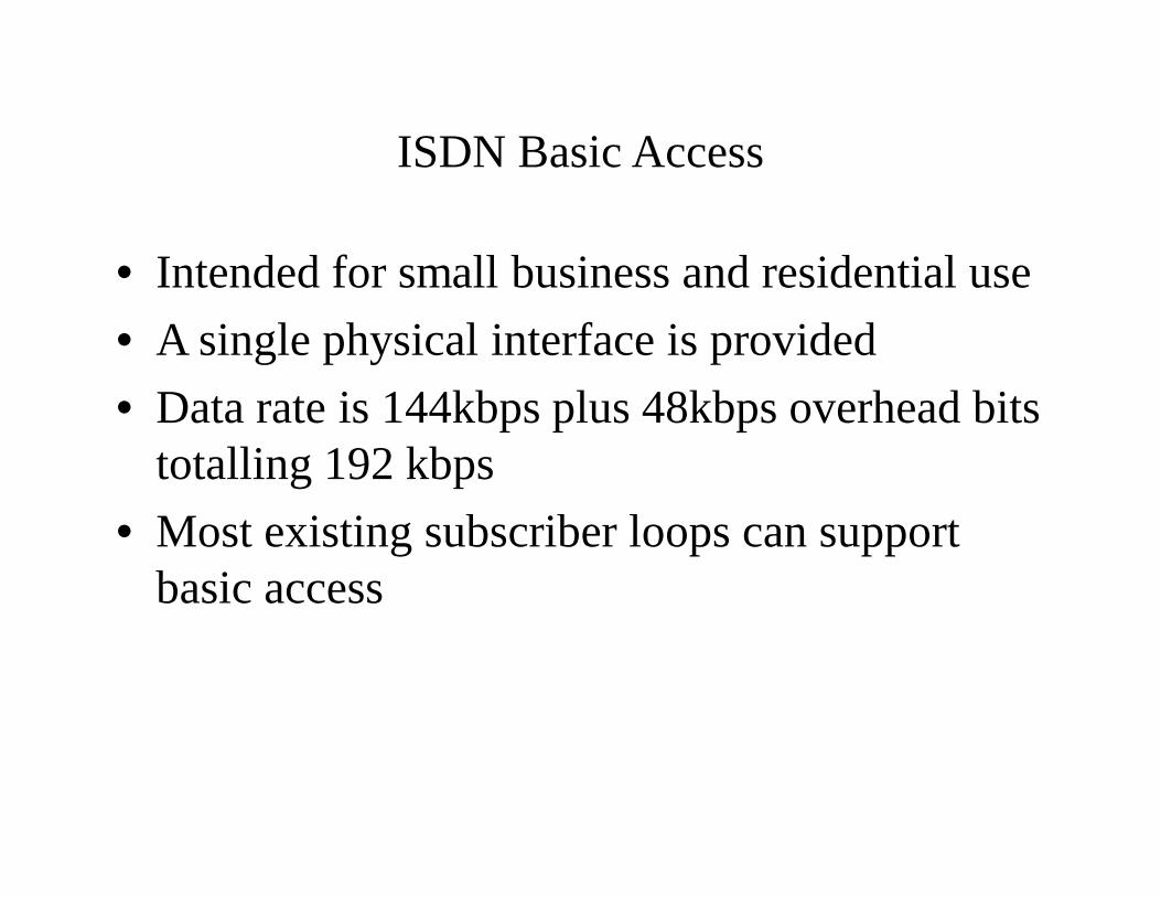
• Intended for small business and residential use• A single physical interface is provided• Data rate is 144kbps plus 48kbps overhead bits
totalling 192 kbps • Most existing subscriber loops can support
basic access
ISDN Primary Access
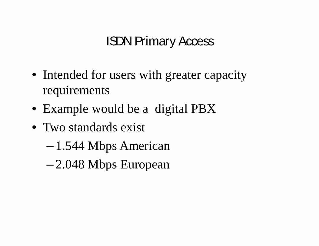
• Intended for users with greater capacity requirements
• Example would be a digital PBX• Two standards exist
– 1.544 Mbps American– 2.048 Mbps European
ISDN Primary Access
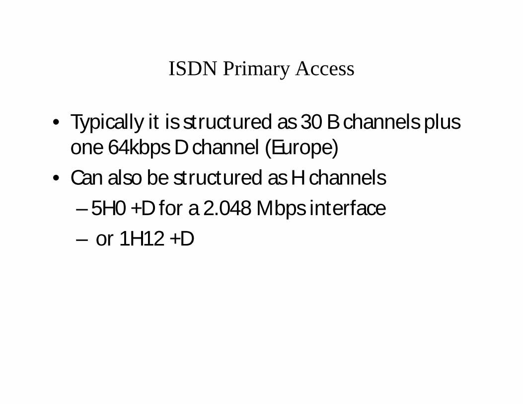
• Typically it is structured as 30 B channels plus one 64kbps D channel (Europe)
• Can also be structured as H channels– 5H0 +D for a 2.048 Mbps interface– or 1H12 +D
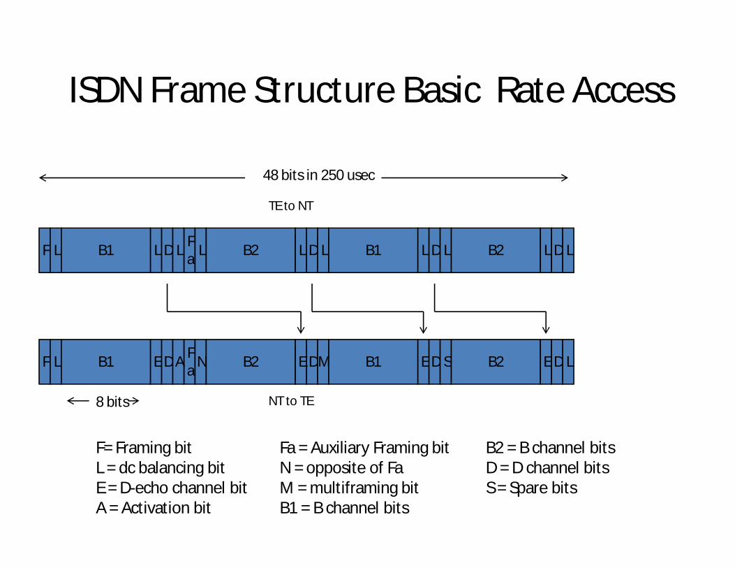
ISDN Frame Structure Basic Rate Access
F L B1 L D FaL L B2 DL L B1 L D L B2 L D L
F L B1 E D FaA N B2 DE M B1 E D S B2 E D L
48 bits in 250 usec
TE to NT
NT to TE8 bits
F= Framing bitL = dc balancing bitE = D-echo channel bitA = Activation bit
Fa = Auxiliary Framing bitN = opposite of FaM = multiframing bitB1 = B channel bits
B2 = B channel bitsD = D channel bitsS = Spare bits
ISDN Contention Resolution
• Several TE’s can share a single line• How is contention resolved? • B-channel Traffic
– No contention as each channel dedicated to particular TE
• D - Channel used for data and control so requires a contention resolution mechanism
D Channel Contention
• Incoming Traffic – LAPD protocol resolves contention
• Outgoing Traffic – Multiple devices share D channel– Contention resolution algorithm required
D Channel Contention
• Idle TEs sends binary 1s on D channel• This means no signal (pseudoternery)• NT echos received binary value back as echo
bit• When NT wishes to send on D channel, it
listens to echo bits• If it hears a string of 1’s equal in length to a
threshold value Xi, it may transmit• Otherwise it must wait
D Channel Contention
• If two TE’s start transmitting simultaneously a collision occurs
• This is detected by each TE by monitoring E bits
• If E bits are identical to D bits sent then no collision
• If discrepency detected TE stops and listens
D Channel Contention
• Priority mechanisms based on threshold values– Control information has priority over user data– When TE has sent data its priority is lowered until
other terminals transmit
D Channel Priorities
• Control Information– Normal Priority X1 =8– Lower Priority X1 =9
• User Data– Normal Priority X2 =10– Lower Priority X2 =11
ISDN Primary Interface
• Multiple channels multiplexed on single medium
• Only point to point configuration is allowed• Typically supports a digital PBX and provides
a synchronous TDM facility
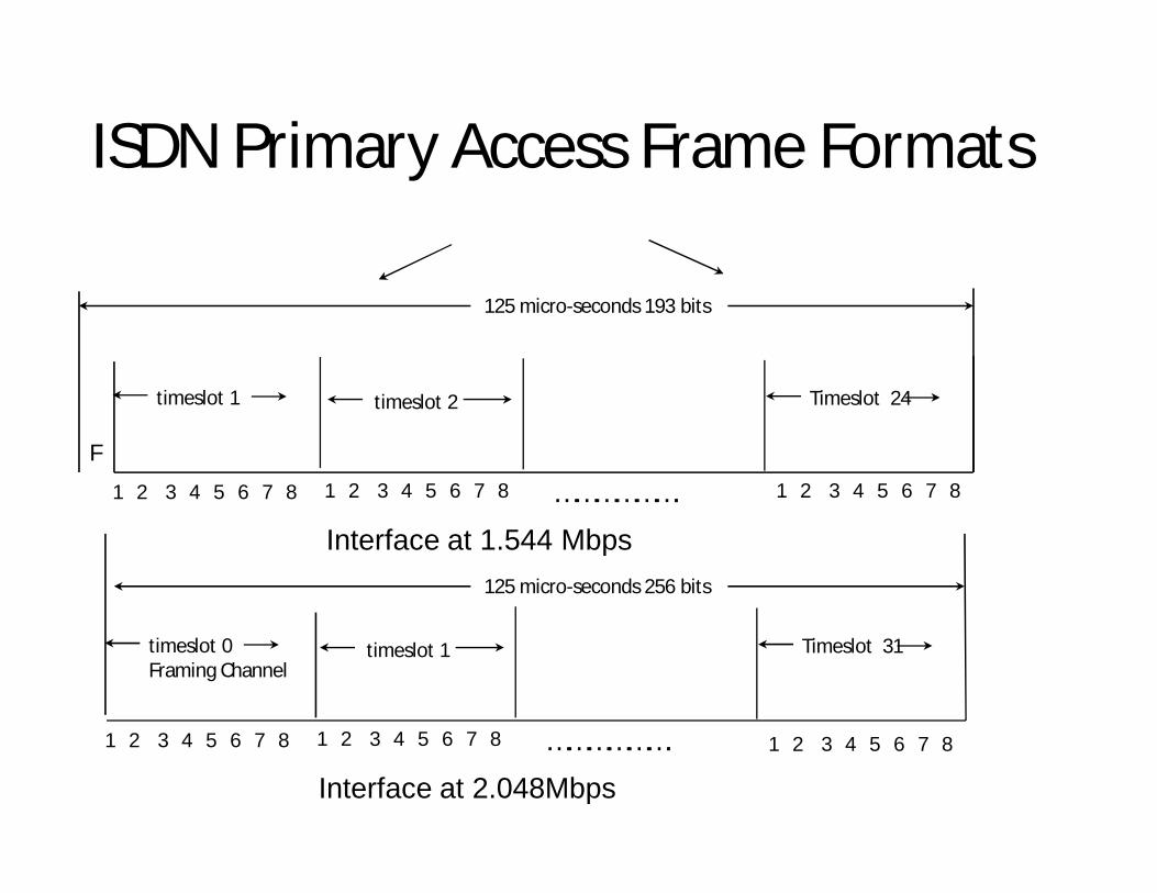
ISDN Primary Access Frame Formats
1 2 3 4 5 6 7 8 1 2 3 4 5 6 7 8 1 2 3 4 5 6 7 8
timeslot 1 timeslot 2 Timeslot 24
……………….F
125 micro-seconds 193 bits
Interface at 1.544 Mbps
1 2 3 4 5 6 7 8 1 2 3 4 5 6 7 8 1 2 3 4 5 6 7 8
timeslot 0Framing Channel
timeslot 1 Timeslot 31
……………….
125 micro-seconds 256 bits
Interface at 2.048Mbps
User Access
• Defined using two concepts– Functional groupings of equipment– Reference points to separate functional
groupings
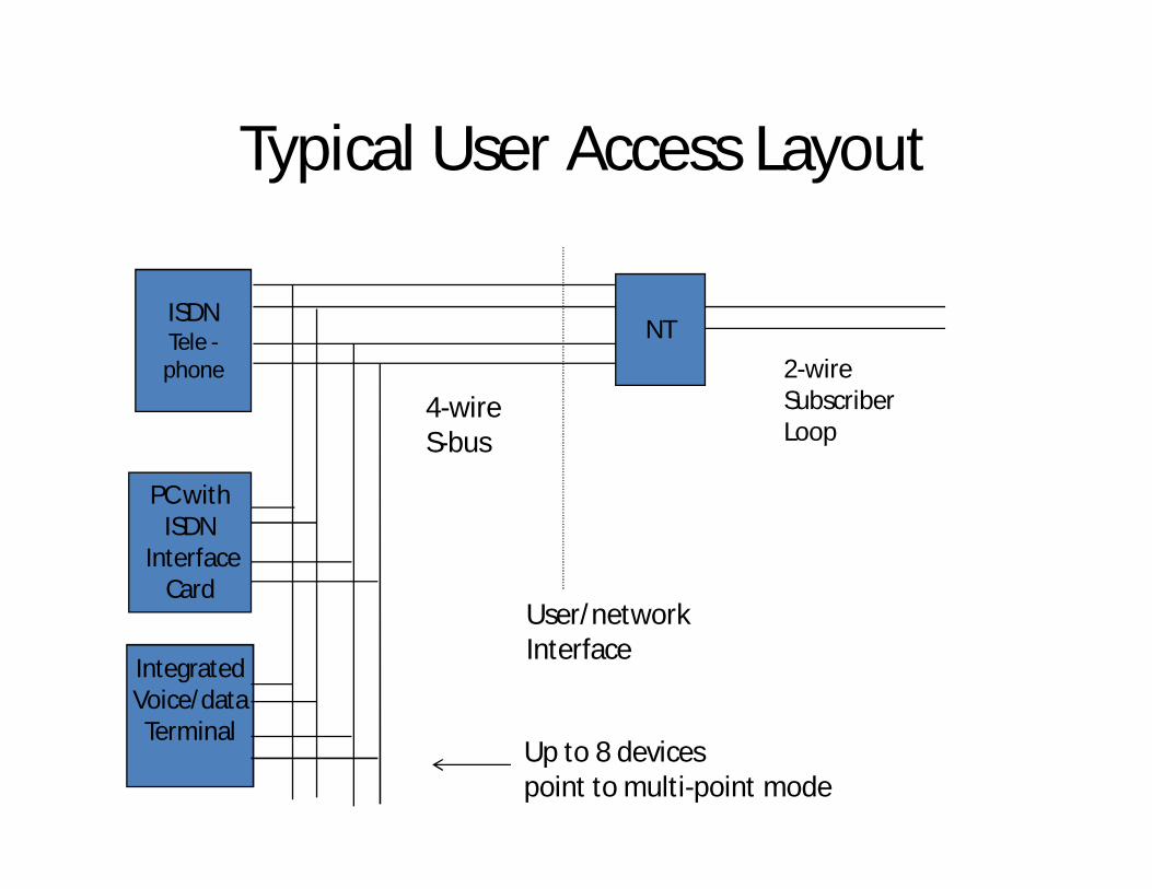
Typical User Access Layout
ISDNTele -phone
PC withISDN
InterfaceCard
NT
IntegratedVoice/dataTerminal
2-wireSubscriberLoop
User/networkInterface
4-wireS-bus
Up to 8 devices point to multi-point mode
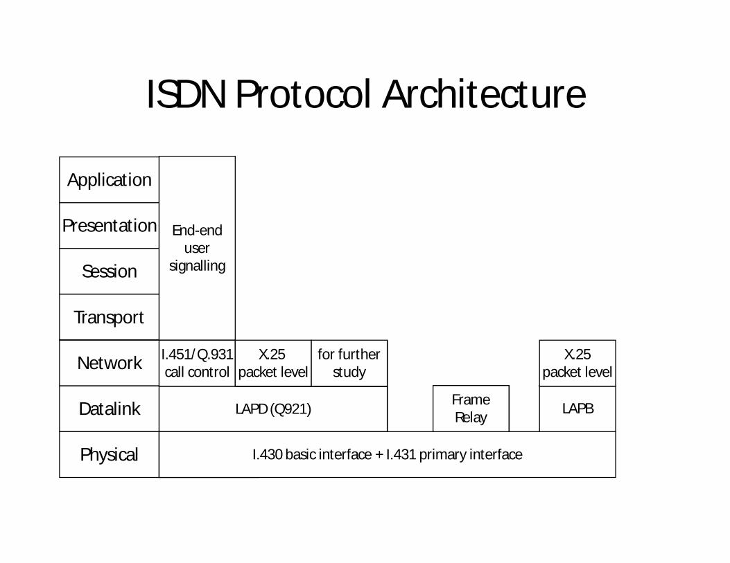
ISDN Protocol Architecture
Application
Presentation
Session
Transport
Network
Datalink
Physical
End-enduser
signalling
Physical
I.451/Q.931call control
LAPD (Q921)
I.430 basic interface + I.431 primary interface
X.25 packet level
for furtherstudy
LAPBFrameRelay
X.25packet level
ISDN Data Link Layer
• Link Access Protocol for the D channel (LAPD) defined for ISDN
• Three applications are supported– Control Signalling– Packet Switching– Telemetry
Network Layer Above LAPD
• Control Signalling– Call Control Protocol (I.451 / Q.931)
• Establishes, maintains and terminates connections on B channels
• Possibility of user - user control signalling above this layer
B-Channel
• Uses– Circuit Switching– Semi-permanent circuits– Packet switching
B-Channel
• Circuit Switching– Circuit is set up on B-channel on demand– D-channel call control protocol is used– Transparent full-duplex digital data path
established between users– Layers 2 to 7 are not visible to ISDN or
specified
B-Channel
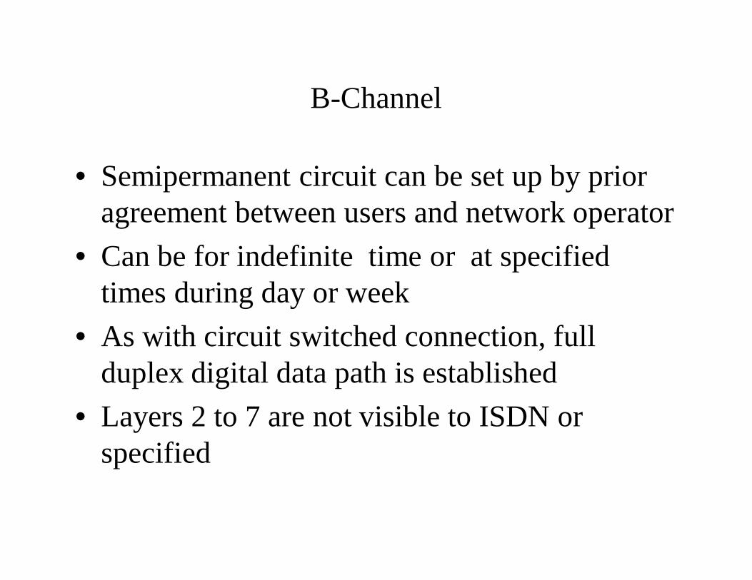
• Semipermanent circuit can be set up by prior agreement between users and network operator
• Can be for indefinite time or at specified times during day or week
• As with circuit switched connection, full duplex digital data path is established
• Layers 2 to 7 are not visible to ISDN or specified
B-Channel Packet Switching
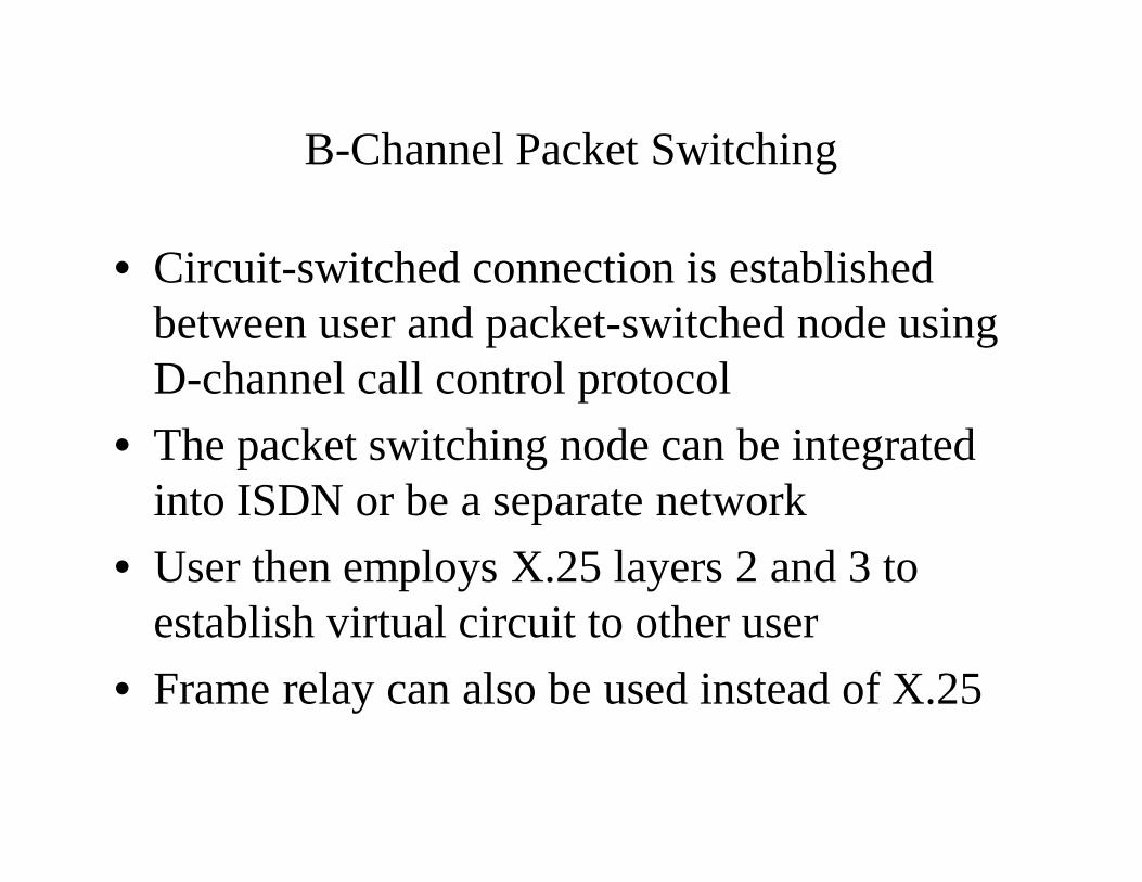
• Circuit-switched connection is established between user and packet-switched node using D-channel call control protocol
• The packet switching node can be integrated into ISDN or be a separate network
• User then employs X.25 layers 2 and 3 to establish virtual circuit to other user
• Frame relay can also be used instead of X.25
D-Channel Packet Switching
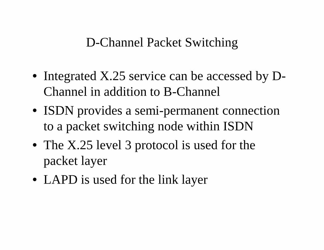
• Integrated X.25 service can be accessed by D-Channel in addition to B-Channel
• ISDN provides a semi-permanent connection to a packet switching node within ISDN
• The X.25 level 3 protocol is used for the packet layer
• LAPD is used for the link layer
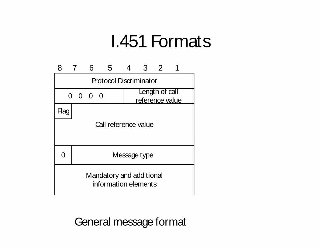
I.451 Formats
0 0 0 0 Length of callreference value
Flag
Call reference value
Protocol Discriminator
Mandatory and additionalinformation elements
Message type
General message format
8 7 6 5 4 3 2 1
0
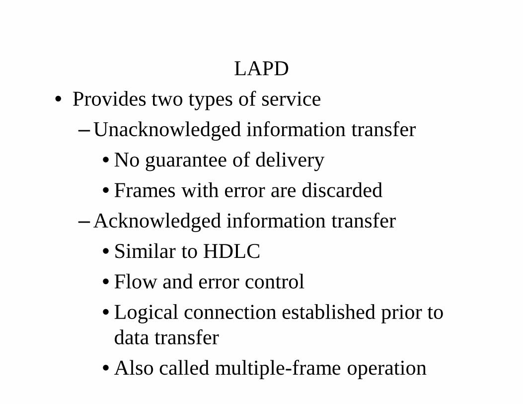
LAPD• Provides two types of service
– Unacknowledged information transfer• No guarantee of delivery• Frames with error are discarded
– Acknowledged information transfer• Similar to HDLC• Flow and error control• Logical connection established prior to
data transfer• Also called multiple-frame operation
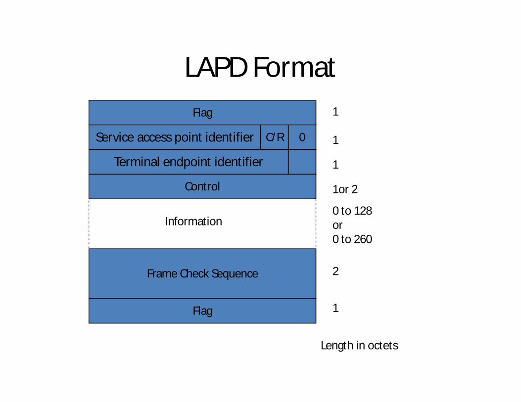
LAPD Format
Terminal endpoint identifier
Service access point identifier C/R 0
Control
Flag
Frame Check Sequence
Flag
Information0 to 128 or0 to 260
1
1
1
1or 2
2
1
Length in octets
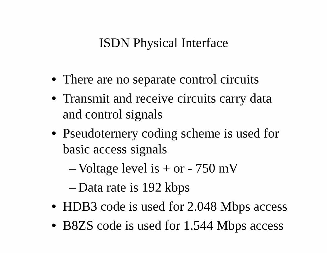
ISDN Physical Interface
• There are no separate control circuits• Transmit and receive circuits carry data
and control signals• Pseudoternery coding scheme is used for
basic access signals– Voltage level is + or - 750 mV– Data rate is 192 kbps
• HDB3 code is used for 2.048 Mbps access• B8ZS code is used for 1.544 Mbps access
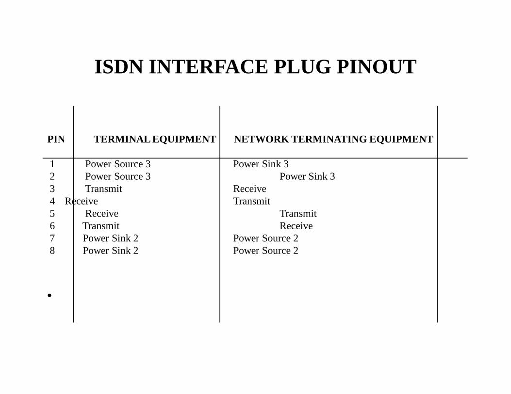
ISDN INTERFACE PLUG PINOUT
PIN TERMINAL EQUIPMENT NETWORK TERMINATING EQUIPMENT
1 Power Source 3 Power Sink 32 Power Source 3 Power Sink 33 Transmit Receive4 Receive Transmit5 Receive Transmit6 Transmit Receive7 Power Sink 2 Power Source 28 Power Sink 2 Power Source 2
•
Broadband ISDN
• Recommendations to support video services as well as normal ISDN services
• Provides user with additional data rates– 155.52 Mbps full-duplex – 155.52 Mbps / 622.08 Mbps– 622.08 Mbps full-duplex
• Exploits optical fibre transmission technology
• Very high performance switches
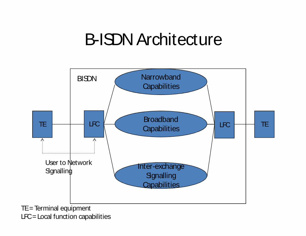
B-ISDN Architecture
TE LFC LFC TE
NarrowbandCapabilities
BroadbandCapabilities
Inter-exchangeSignalling
Capabilities
BISDN
User to NetworkSignalling
TE = Terminal equipmentLFC = Local function capabilities
B-ISDN
• ATM is specified for Information transfer across the user-network interface
• Fixed size 53 octet packet with a 5 octet header
• Implies that internal switching will be packet-based
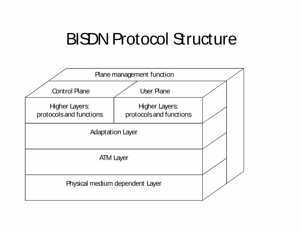
BISDN Protocol Structure
Higher Layers:protocols and functions
Higher Layers:protocols and functions
Adaptation Layer
ATM Layer
Physical medium dependent Layer
Plane management function
Control Plane User Plane
UNIT II - ISDN PROTOCOL ARCHITECTURE AND SIGNALING
ISDN and the OSI Reference Model
• The ISDN Physical Layer• The ISDN Data Link Layer• The ISDN Network Layer
ISDN Protocols
• E-series protocols—Telephone network standards for ISDN.
• I-series protocols—Specify ISDN concepts and interfaces.
• Q-series protocols—Standards for ISDN switching and signaling.
• Operate at the physical, data link, and network layers of the OSI reference model
ISDN Protocol Operating OSI Layers 1 Through 3
• Physical layer ISDN protocols– BRI (ITU-T I.430) / PRI (ITU-T I.431)
• Defines two ISDN physical layer frame formats
–Inbound (local exchange to ISDN customer)
–Outbound (ISDN customer to local exchange )
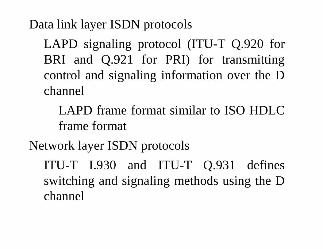
Data link layer ISDN protocolsLAPD signaling protocol (ITU-T Q.920 forBRI and Q.921 for PRI) for transmittingcontrol and signaling information over the Dchannel
LAPD frame format similar to ISO HDLCframe format
Network layer ISDN protocolsITU-T I.930 and ITU-T Q.931 definesswitching and signaling methods using the Dchannel
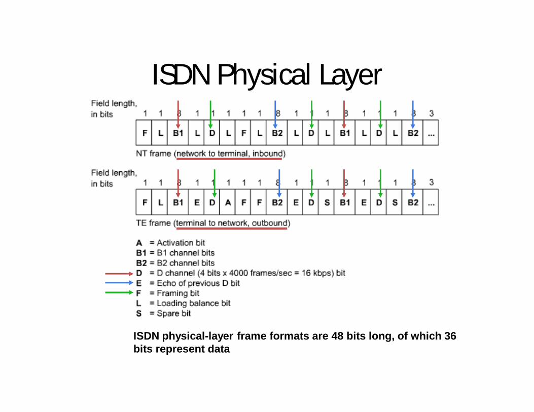
ISDN Physical Layer
ISDN physical-layer frame formats are 48 bits long, of which 36 bits represent data
D Channel
• When a TCP connection is established, there is an exchange of information called the connection setup. – This information is exchanged over the path
on which the data will eventually be transmitted.
– Both the control information and the data share the same pathway.
– This is called in-band signaling. • ISDN however, uses a separate channel for
control information, the D channel.
•The D channel carries signaling messages, such as call setup and teardown, to control calls on B channels. •Traffic over the D channel employs the Link Access Procedure on the D Channel (LAPD) protocol. •LAPD is a data link layer protocol based on HDLC.
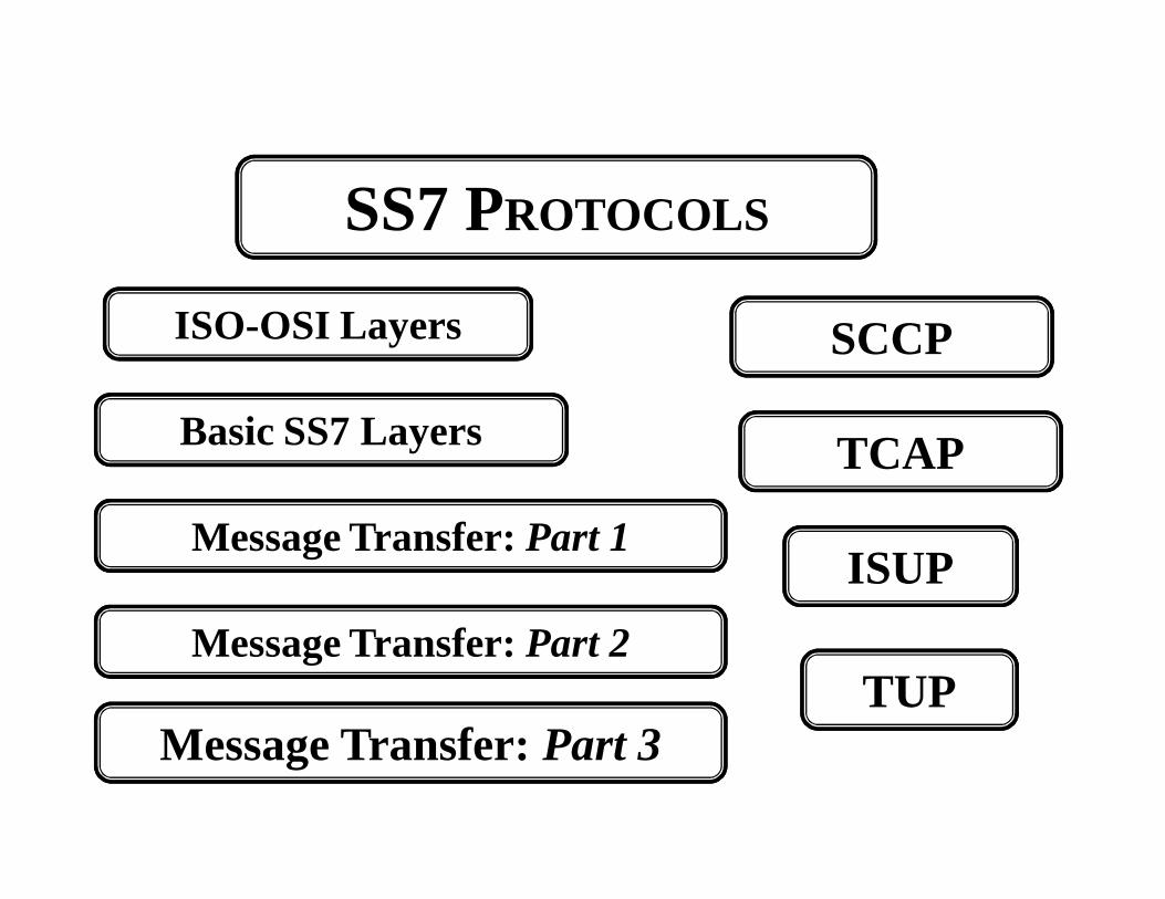
SS7 PROTOCOLS
Basic SS7 Layers
ISO-OSI Layers
Message Transfer: Part 1
TUPMessage Transfer: Part 2
Message Transfer: Part 3
ISUP
TCAP
SCCP
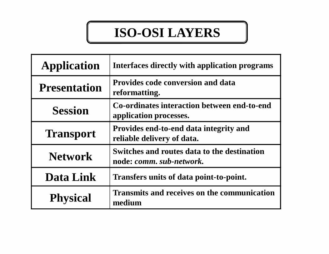
ISO-OSI LAYERS
Application Interfaces directly with application programs
Presentation Provides code conversion and data reformatting.
Session Co-ordinates interaction between end-to-end application processes.
Transport Provides end-to-end data integrity and reliable delivery of data.
Network Switches and routes data to the destination node: comm. sub-network.
Data Link Transfers units of data point-to-point.
Physical Transmits and receives on the communication medium
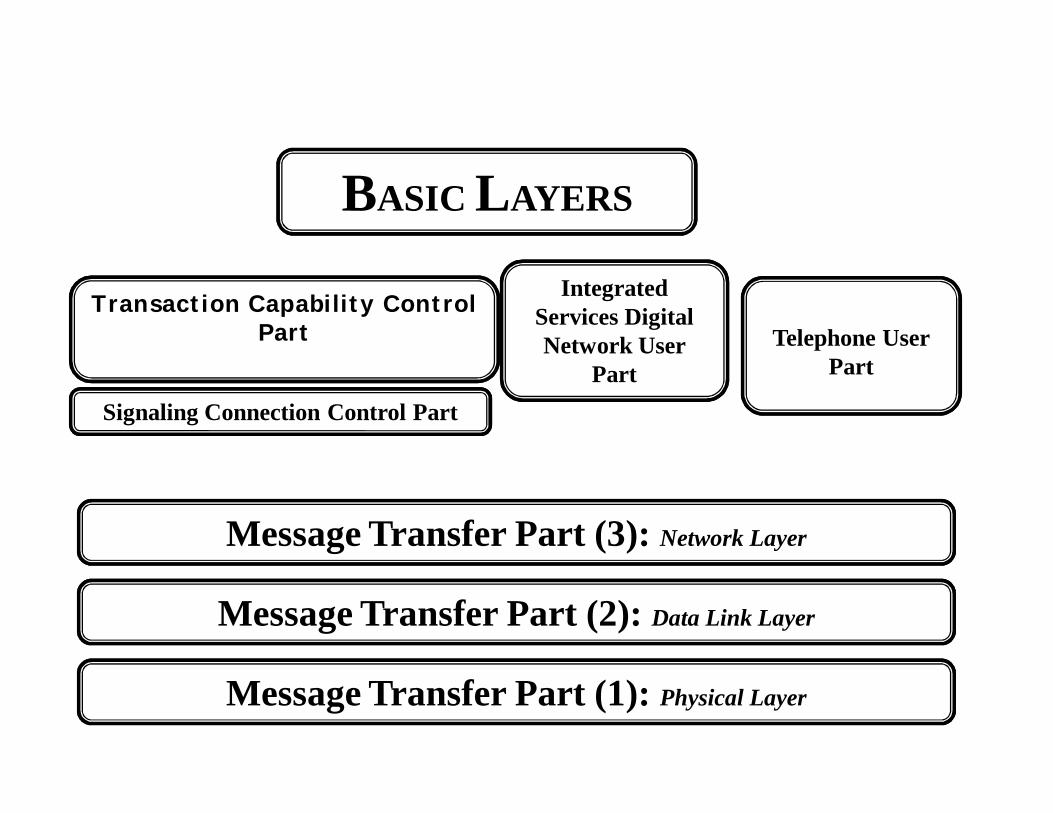
BASIC LAYERS
Signaling Connection Control Part
Message Transfer Part (1): Physical Layer
Message Transfer Part (2): Data Link Layer
Message Transfer Part (3): Network Layer
Transaction Capability Control Part
Integrated Services Digital Network User
PartTelephone User
Part
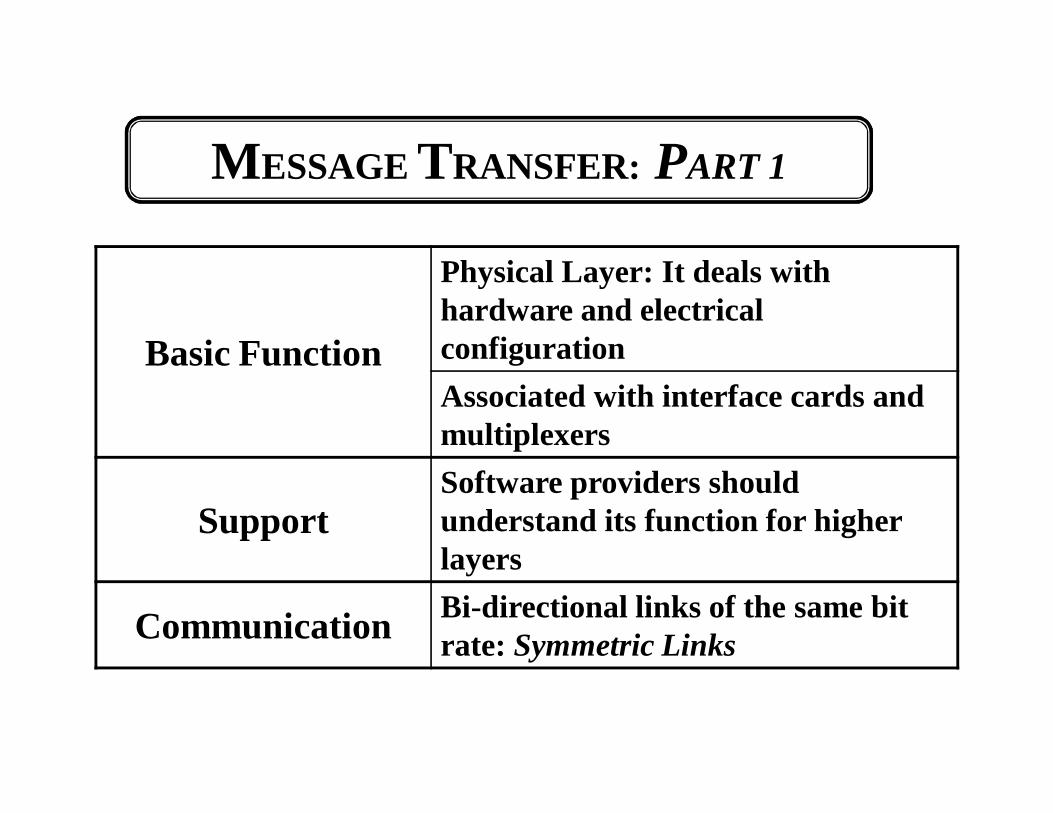
MESSAGE TRANSFER: PART 1
Basic Function
Physical Layer: It deals with hardware and electrical configurationAssociated with interface cards and multiplexers
SupportSoftware providers should understand its function for higher layers
Communication Bi-directional links of the same bit rate: Symmetric Links
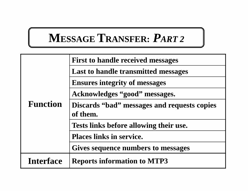
MESSAGE TRANSFER: PART 2
Function
First to handle received messagesLast to handle transmitted messagesEnsures integrity of messagesAcknowledges “good” messages.Discards “bad” messages and requests copies of them.Tests links before allowing their use.Places links in service.Gives sequence numbers to messages
Interface Reports information to MTP3
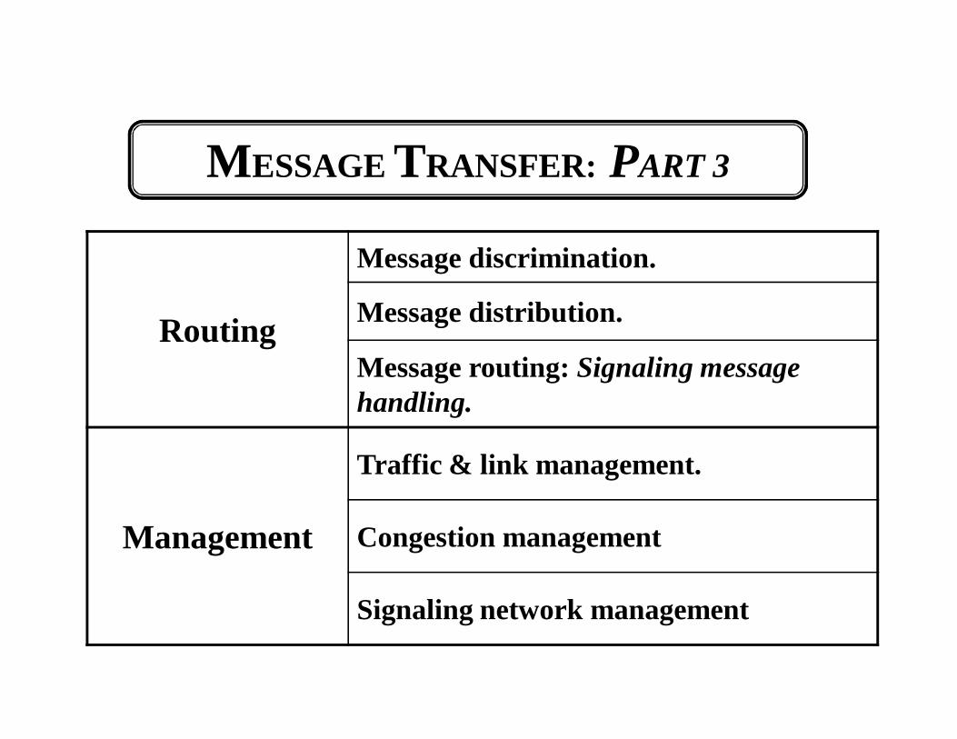
MESSAGE TRANSFER: PART 3
Routing
Message discrimination.
Message distribution.
Message routing: Signaling message handling.
Management
Traffic & link management.
Congestion management
Signaling network management
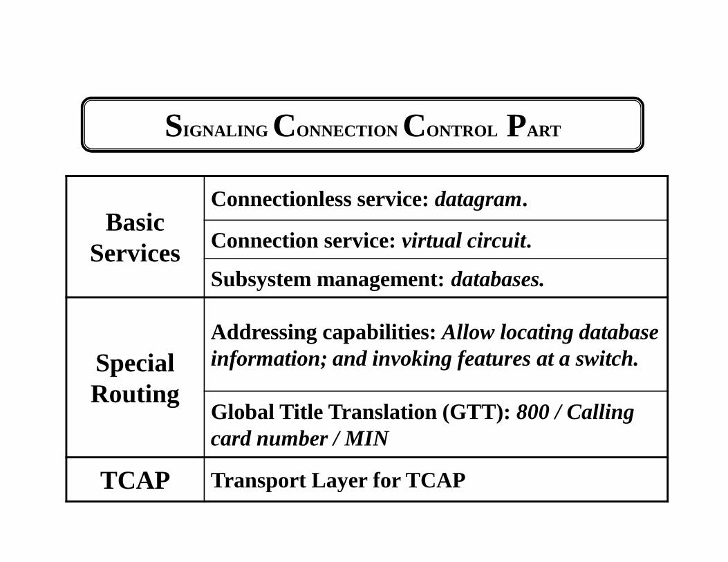
SIGNALING CONNECTION CONTROL PART
Basic Services
Connectionless service: datagram.
Connection service: virtual circuit.
Subsystem management: databases.
Special Routing
Addressing capabilities: Allow locating database information; and invoking features at a switch.
Global Title Translation (GTT): 800 / Calling card number / MIN
TCAP Transport Layer for TCAP
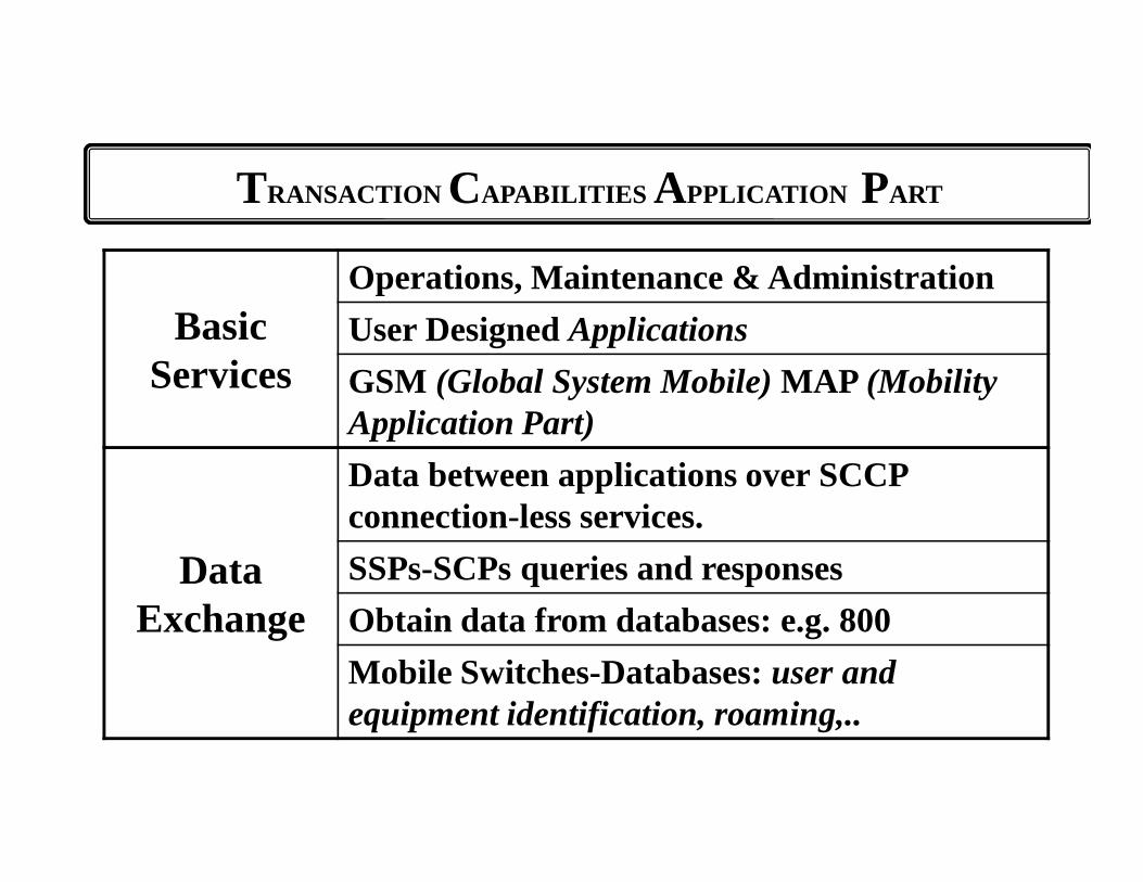
TRANSACTION CAPABILITIES APPLICATION PART
Basic Services
Operations, Maintenance & AdministrationUser Designed ApplicationsGSM (Global System Mobile) MAP (Mobility Application Part)
Data Exchange
Data between applications over SCCP connection-less services.SSPs-SCPs queries and responsesObtain data from databases: e.g. 800Mobile Switches-Databases: user and equipment identification, roaming,..
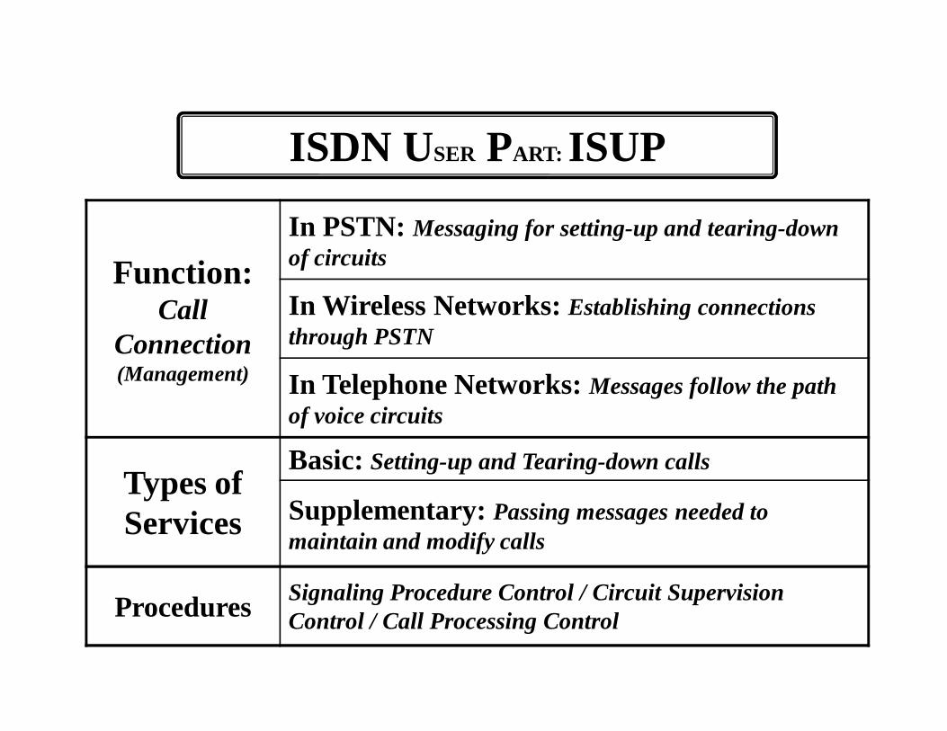
ISDN USER PART: ISUP
Function: Call
Connection (Management)
In PSTN: Messaging for setting-up and tearing-down of circuits
In Wireless Networks: Establishing connections through PSTN
In Telephone Networks: Messages follow the path of voice circuits
Types of Services
Basic: Setting-up and Tearing-down calls
Supplementary: Passing messages needed to maintain and modify calls
Procedures Signaling Procedure Control / Circuit Supervision Control / Call Processing Control
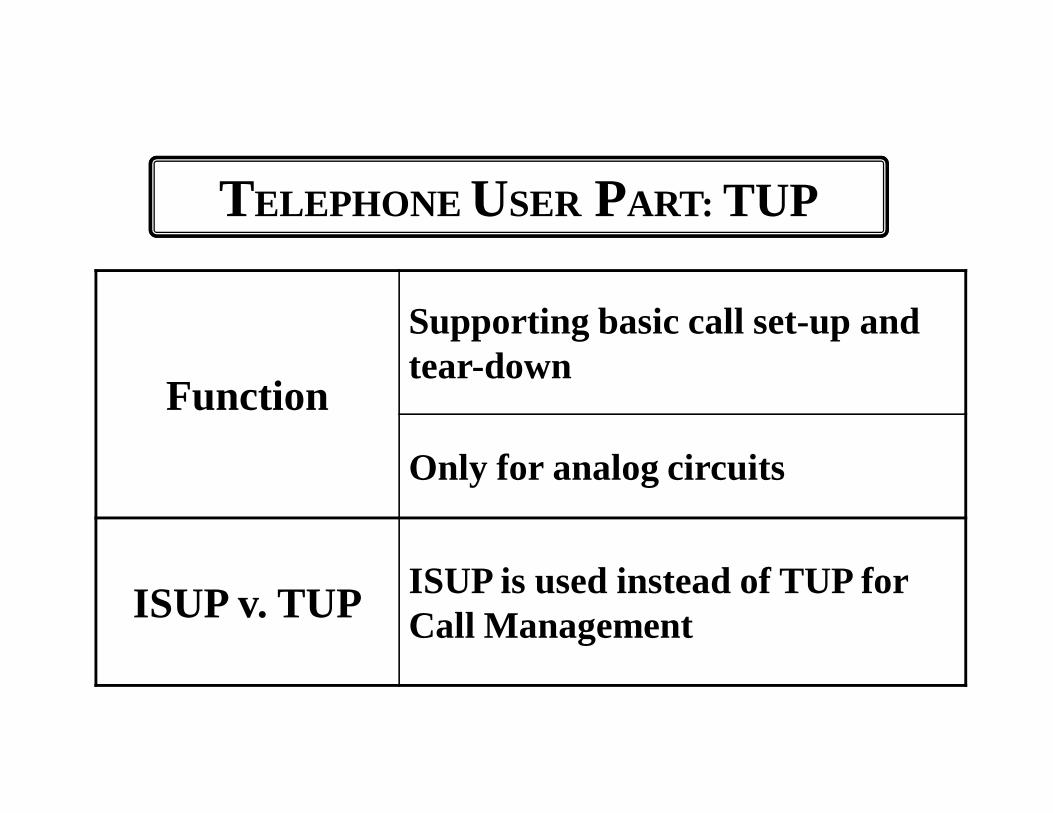
TELEPHONE USER PART: TUP
Function
Supporting basic call set-up and tear-down
Only for analog circuits
ISUP v. TUP ISUP is used instead of TUP for Call Management
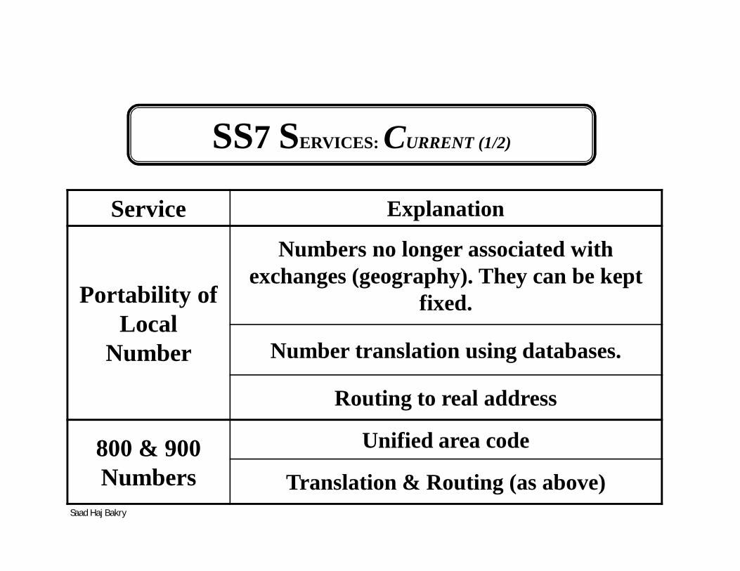
SS7 SERVICES: CURRENT (1/2)
Saad Haj Bakry
Service Explanation
Portability of Local
Number
Numbers no longer associated with exchanges (geography). They can be kept
fixed.
Number translation using databases.
Routing to real address
800 & 900 Numbers
Unified area code
Translation & Routing (as above)

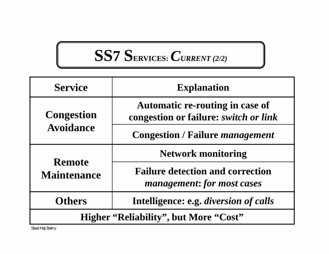
SS7 SERVICES: CURRENT (2/2)
Saad Haj Bakry
Service Explanation
Congestion Avoidance
Automatic re-routing in case of congestion or failure: switch or link
Congestion / Failure management
Remote Maintenance
Network monitoring
Failure detection and correction management: for most cases
Others Intelligence: e.g. diversion of callsHigher “Reliability”, but More “Cost”

SS7 SERVICES: CURRENT (1/2)
Saad Haj Bakry
Service Explanation
Portability of Local
Number
Numbers no longer associated with exchanges (geography). They can be kept
fixed.
Number translation using databases.
Routing to real address
800 & 900 Numbers
Unified area code
Translation & Routing (as above)
SS7 SERVICES: CURRENT (2/2)
Saad Haj Bakry
Service Explanation
Congestion Avoidance
Automatic re-routing in case of congestion or failure: switch or link
Congestion / Failure management
Remote Maintenance
Network monitoring
Failure detection and correction management: for most cases
Others Intelligence: e.g. diversion of callsHigher “Reliability”, but More “Cost”
Using ISDN for IP Data Networks
• Characteristics– Speed– Fast call setup– Bandwidth on Demand
Using ISDN for IP Data Networks
• Modes of Usage– Dial Up (LAN or host)– Bandwidth on Demand – Backup lines– Permanent connections
ISDN, CEENet Workshop '97, Zagreb, August '97 90
Dial Up
• Providers need:– subscribe for PRI connections or multiple
BRI connections– ISDN Access Server
ISDN Access Servers
• Digital modems (accepting analog and ISDN calls)– software busy-out feature
• 56 kbit/s technologies• Rate adaption (V.110, V.120,..)• Compression (Stac,..)• Synchronous PPP (with CHAP/PAP
authentication)
ISDN Access Servers 2
• PPP Multilink• BACP• Controlling the number of B-channels per user• D-channel based callback• CLIP - Caller Line Identification Presentation
ISDN, CEENet Workshop '97, Zagreb, August '97 93
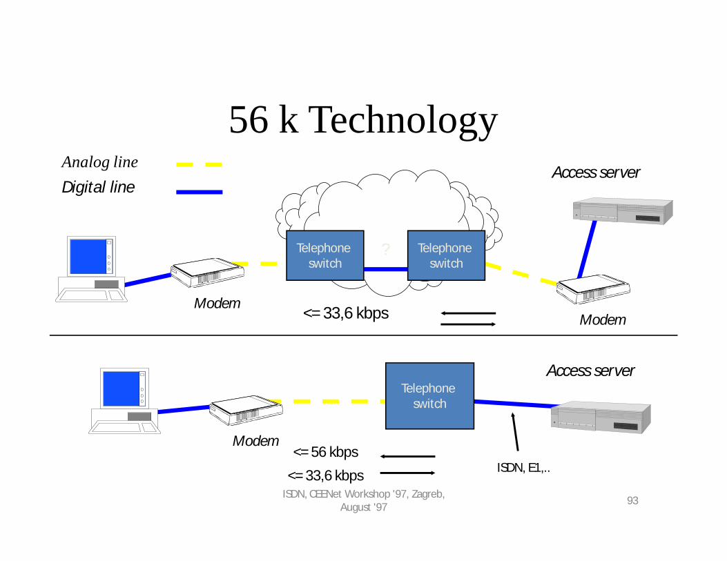
56 k TechnologyAccess server
Modem
Telephone switch
Telephone switch
Telephone switch
?
Access server
Modem
Modem
Digital lineAnalog line
<= 33,6 kbps
<= 56 kbpsISDN, E1,..<= 33,6 kbps
56 k Prerequisites
• Only one analogue/digital conversion– less noise and faster digital lines
• Digital Access Server • Same technology in Access Server and in dial-
up modem – K56Flex from Lucent Technologies and
Rocwell– X2 from U.S. Robotics, Texas Instruments
and Cirrus Logic
56 k Considerations
• 56 k not reached in reality– 43 kbps practical maximum
• Cost for upgrading equipment to ITU standard
Dial Up
• Users need for host connections:– subscribe for BRI connection– ISDN Adapter
• Users need for LAN connections– subscribe for PRI or BRI connection– ISDN router (commercial, PC version with
ISDN Adapter,..)
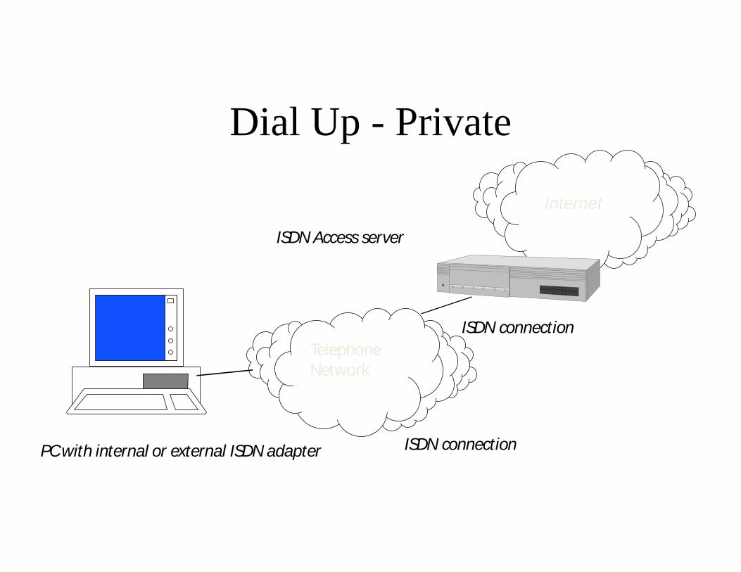
Dial Up - Private
PC with internal or external ISDN adapter
Internet
ISDN Access server
ISDN connection
ISDN connectionTelephone Network
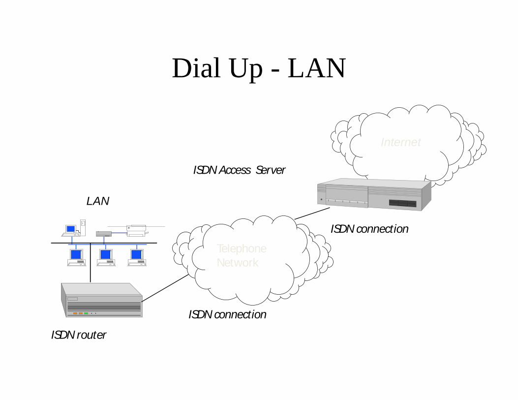
Dial Up - LAN
ISDN connection
ISDN connection
ISDN router
Internet
LAN
ISDN Access Server
Telephone Network
ISDN Adapters
• Internal/external• Active/passive (for internal)• Integrated NT• Plug for telephone line• Integrated modem• Synchronous PPP (with CHAP/PAP
authentication)
ISDN Adapters 2
• PPP Multilink• Rate adaption (V.110, V.120,..)• CAPI• Compression (Stac,…)
ISDN Routers
• Integrated NT• Plug for telephone line• Integrated modem• Synchronous PPP (with CHAP/PAP
authentication)• PPP Multilink• Compression (Stac,…)• Tarrif management
Bandwidth on Demand
• Router to router connections • ISDN call setup when leased line overloaded
Backup lines
• Router to router connections• ISDN call setup when leased line fails
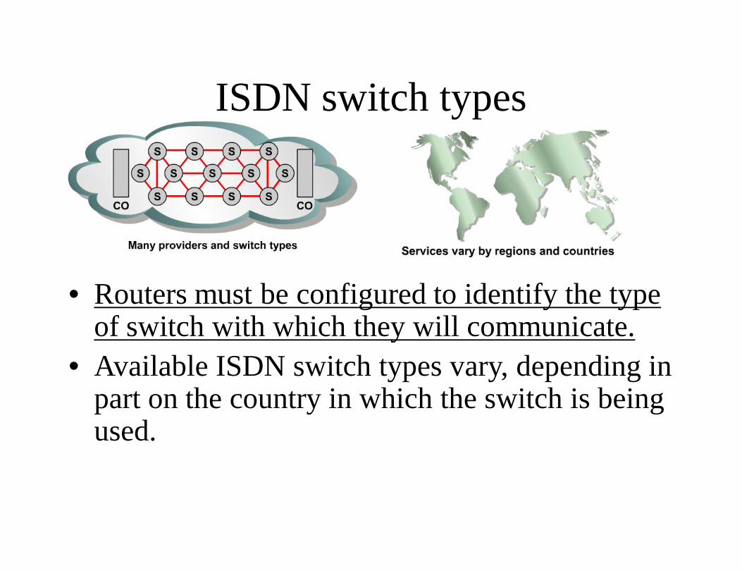
ISDN switch types
• Routers must be configured to identify the type of switch with which they will communicate.
• Available ISDN switch types vary, depending in part on the country in which the switch is being used.
As a consequence of various implementations ofQ.931, the D channel signaling protocol used onISDN switches varies from vendor to vendor.Before the router can be connected to an ISDNservice, it must be configured for the switch typeused at the CO.This information must be specified during routerconfiguration.
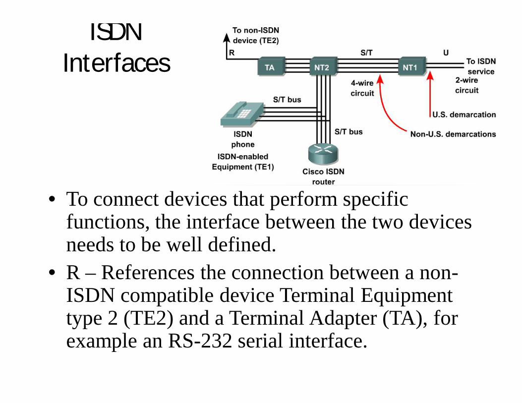
ISDN Interfaces
• To connect devices that perform specific functions, the interface between the two devices needs to be well defined.
• R – References the connection between a non-ISDN compatible device Terminal Equipment type 2 (TE2) and a Terminal Adapter (TA), for example an RS-232 serial interface.
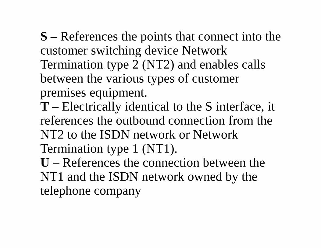
S – References the points that connect into the customer switching device Network Termination type 2 (NT2) and enables calls between the various types of customer premises equipment. T – Electrically identical to the S interface, it references the outbound connection from the NT2 to the ISDN network or Network Termination type 1 (NT1). U – References the connection between the NT1 and the ISDN network owned by the telephone company
UNIT III - BROAD BAND ISDN
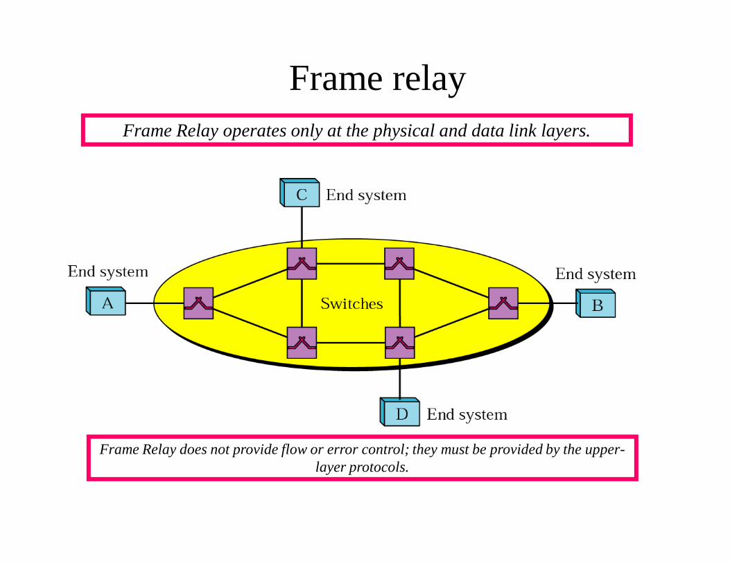
Frame relayFrame Relay operates only at the physical and data link layers.
Frame Relay does not provide flow or error control; they must be provided by the upper-layer protocols.
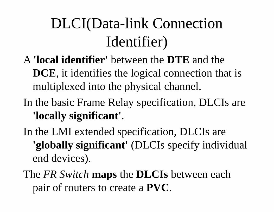
A 'local identifier' between the DTE and the DCE, it identifies the logical connection that is multiplexed into the physical channel.
In the basic Frame Relay specification, DLCIs are 'locally significant'.
In the LMI extended specification, DLCIs are 'globally significant' (DLCIs specify individual end devices).
The FR Switch maps the DLCIs between each pair of routers to create a PVC.
DLCI(Data-link Connection Identifier)

Frame Relay-Interface types
• UNI: User-|Network Interface• NNI: Network-Network Interface
Frame Relaynetwork
Frame Relaynetwork
Frame Relaynetworkuser user
UNI UNINNI NNIPVC segment
Multi-network PVC
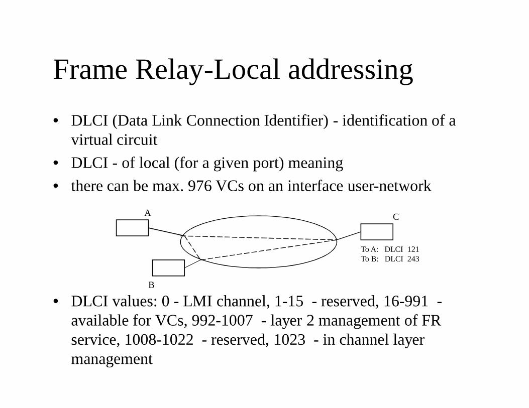
Frame Relay-Local addressing• DLCI (Data Link Connection Identifier) - identification of a
virtual circuit• DLCI - of local (for a given port) meaning• there can be max. 976 VCs on an interface user-network
• DLCI values: 0 - LMI channel, 1-15 - reserved, 16-991 -available for VCs, 992-1007 - layer 2 management of FR service, 1008-1022 - reserved, 1023 - in channel layer management
A
B
C
To A: DLCI 121To B: DLCI 243
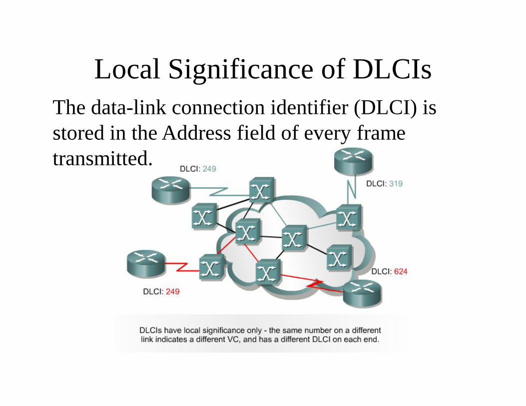
Local Significance of DLCIsThe data-link connection identifier (DLCI) is stored in the Address field of every frame transmitted.
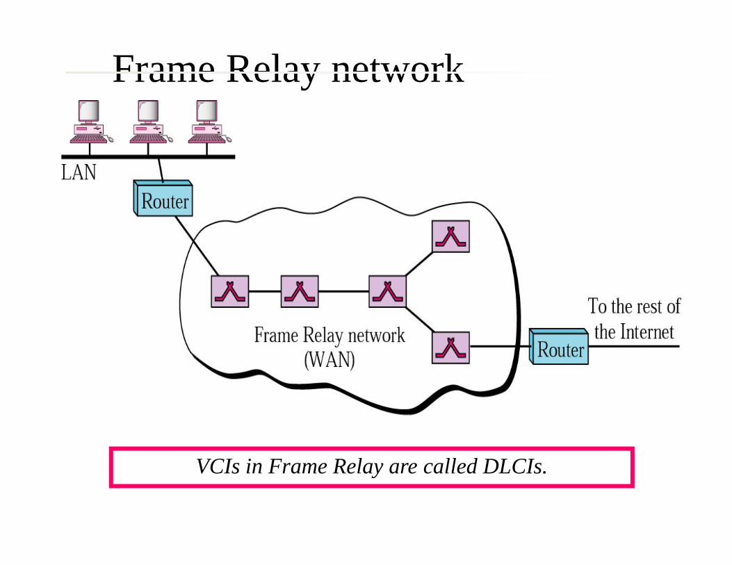
Frame Relay network
VCIs in Frame Relay are called DLCIs.
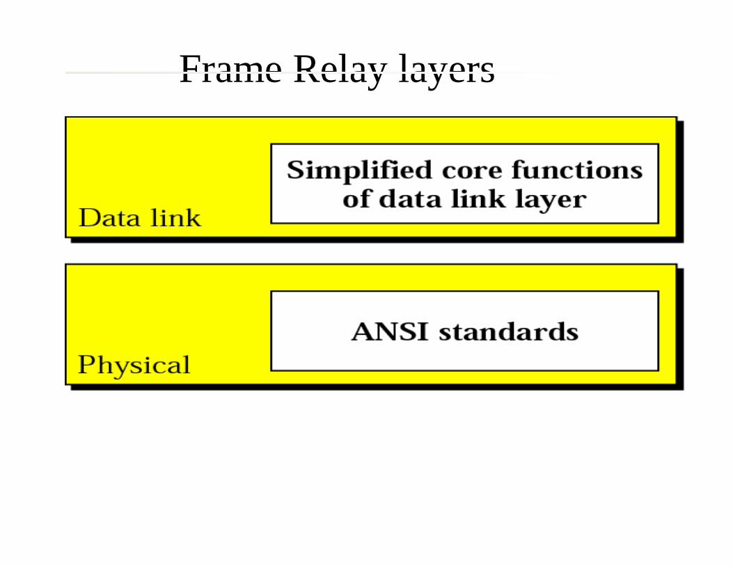
Frame Relay layers
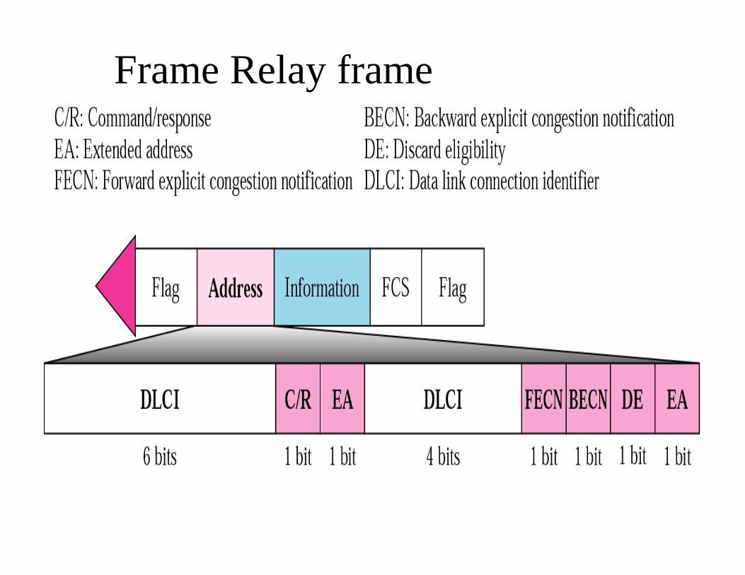
Frame Relay frame
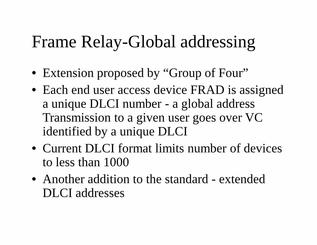
Frame Relay-Global addressing
• Extension proposed by “Group of Four”• Each end user access device FRAD is assigned
a unique DLCI number - a global addressTransmission to a given user goes over VC identified by a unique DLCI
• Current DLCI format limits number of devices to less than 1000
• Another addition to the standard - extended DLCI addresses
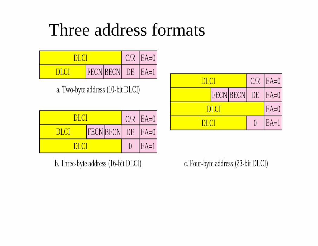
Three address formats
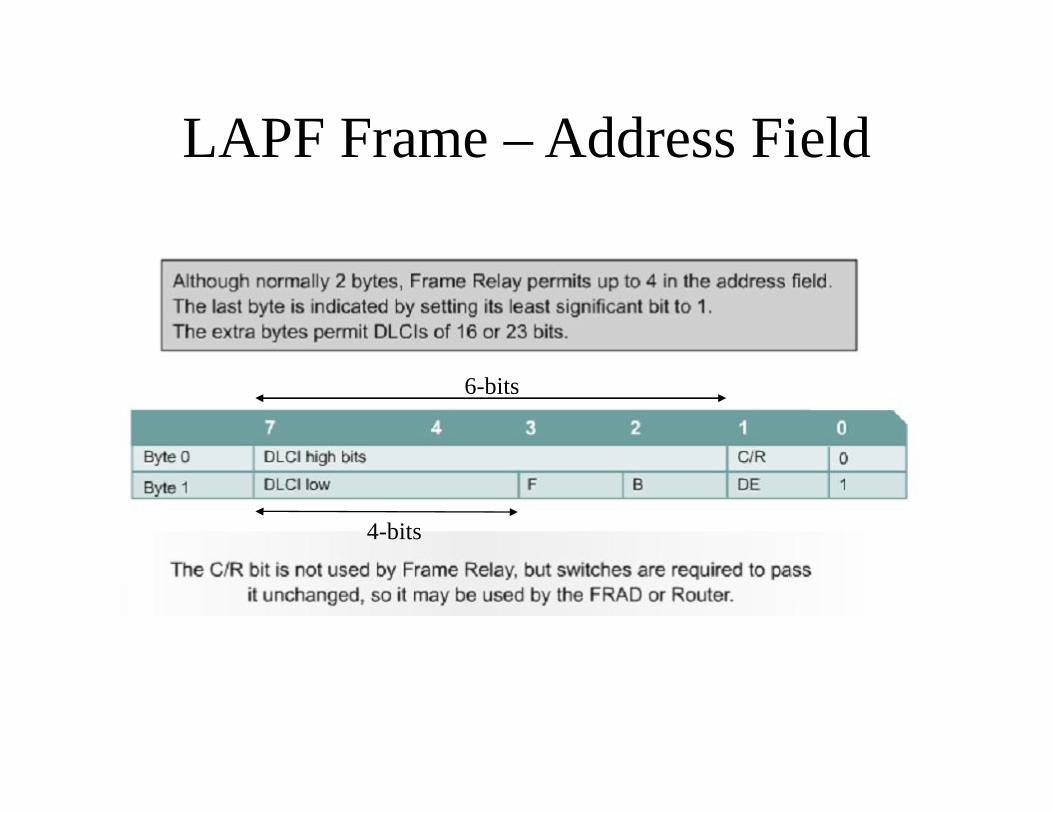
LAPF Frame – Address Field
6-bits
4-bits
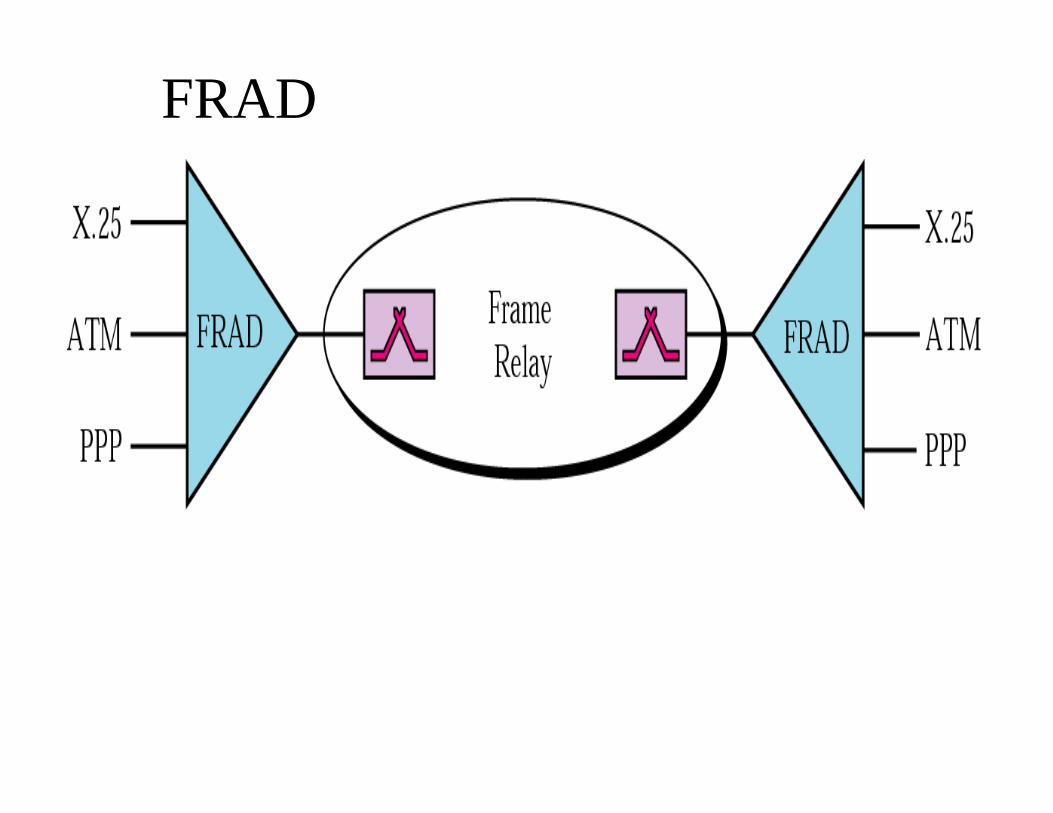
FRAD
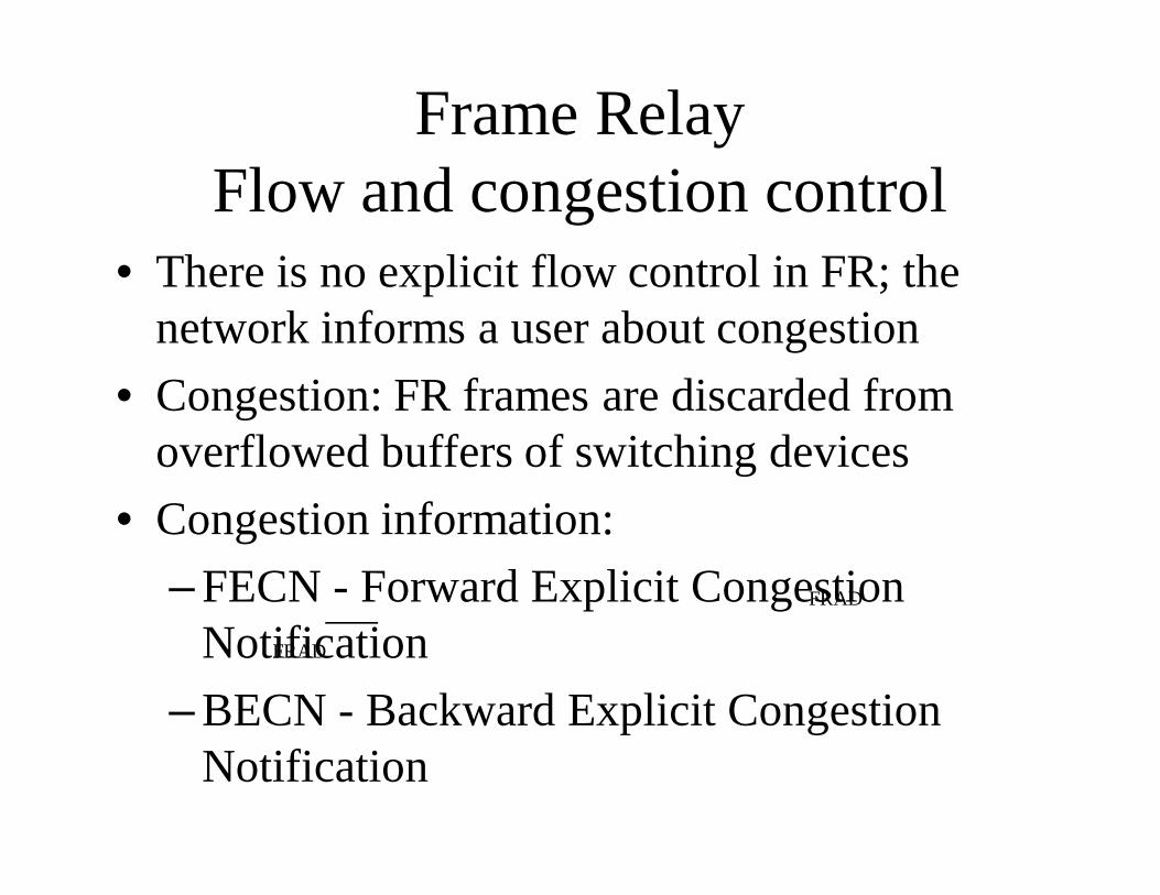
Frame RelayFlow and congestion control
• There is no explicit flow control in FR; the network informs a user about congestion
• Congestion: FR frames are discarded from overflowed buffers of switching devices
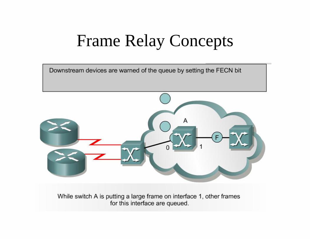
• Congestion information:– FECN - Forward Explicit Congestion
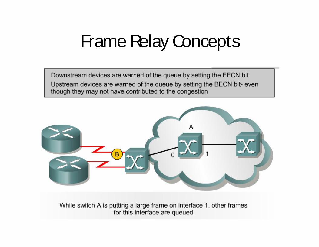
Notification– BECN - Backward Explicit Congestion
Notification
FRAD
FRAD
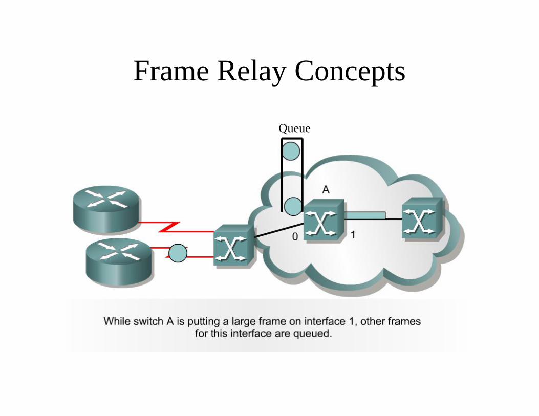
Frame Relay Concepts
Queue
Frame Relay Concepts
Frame Relay Concepts
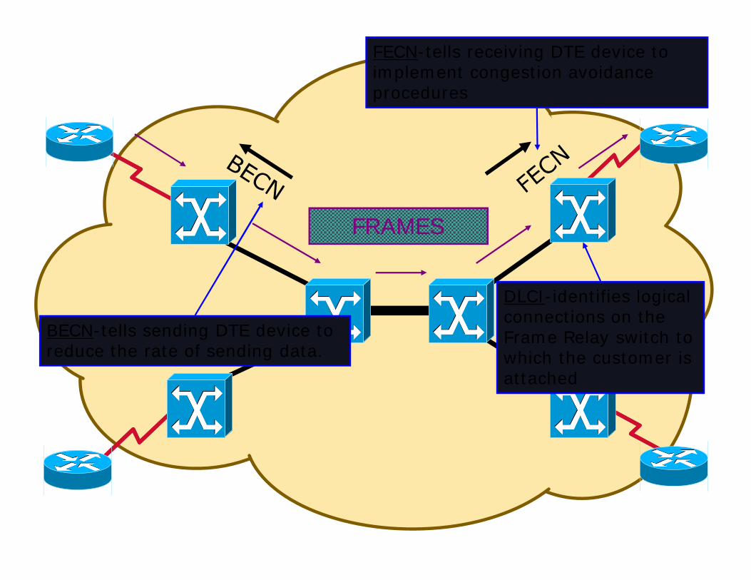
DLCI-identifies logical connections on the Frame Relay switch to which the customer is attached
BECN-tells sending DTE device to reduce the rate of sending data.
FECN-tells receiving DTE device to implement congestion avoidance procedures
FRAMES
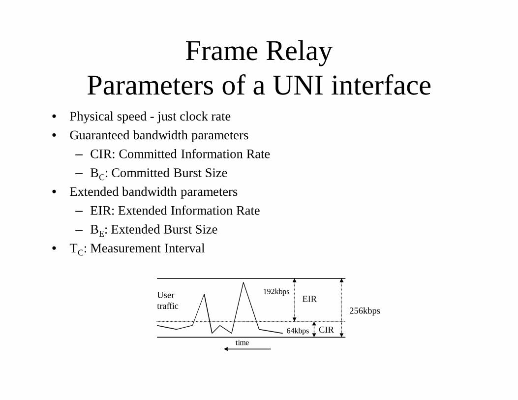
Frame RelayParameters of a UNI interface
• Physical speed - just clock rate• Guaranteed bandwidth parameters
– CIR: Committed Information Rate– BC: Committed Burst Size
• Extended bandwidth parameters– EIR: Extended Information Rate– BE: Extended Burst Size
• TC: Measurement Interval
Usertraffic
192kbps
64kbps
EIR
CIR
256kbps
time
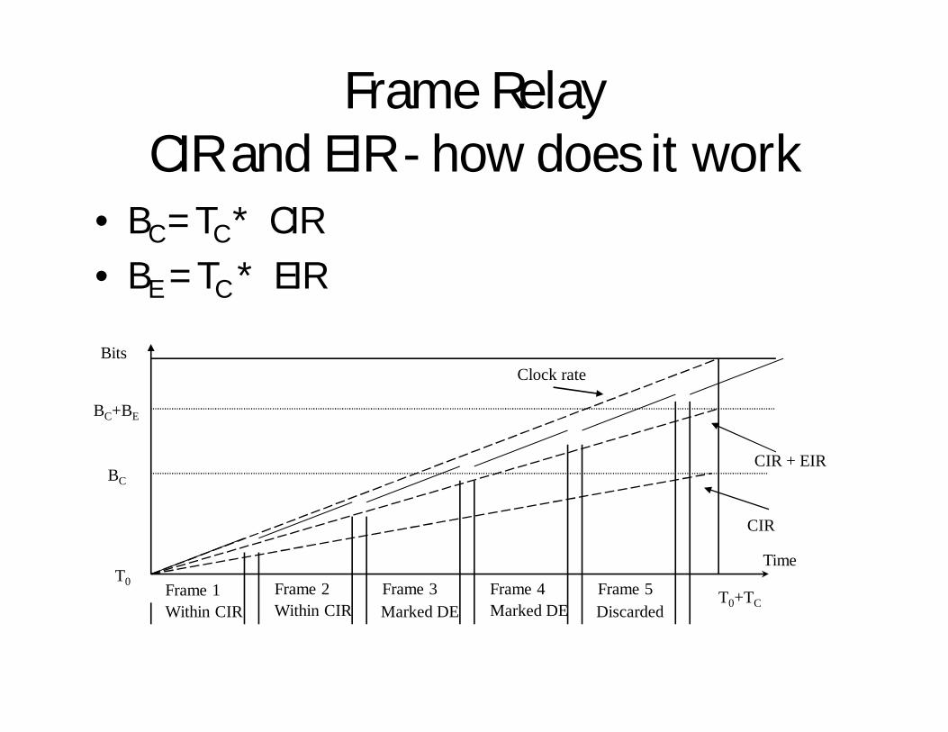
Frame RelayCIR and EIR - how does it work
• BC = TC * CIR• BE = TC * EIR
Frame 1 Frame 2 Frame 3 Frame 4 Frame 5Within CIR Within CIR Marked DE Marked DE Discarded
Bits
BC+BE
BC
T0T0+TC
Time
CIR
CIR + EIR
Clock rate
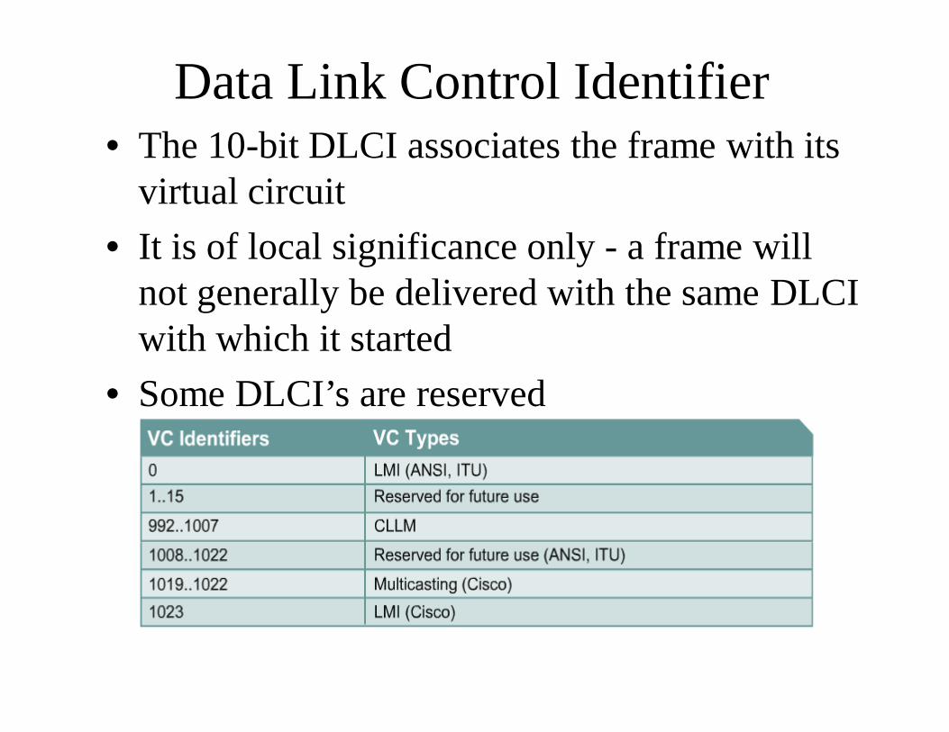
Data Link Control Identifier• The 10-bit DLCI associates the frame with its
virtual circuit• It is of local significance only - a frame will
not generally be delivered with the same DLCI with which it started
• Some DLCI’s are reserved
Frame Relay Local Management Interface - LMI• LMI - a signaling protocol used on an
interface: end user - network (UNI)• Implementation optional (everybody
implements it...)• Usage:
– notification about: creation, deletion, existence of PVCs on a given port
– notification about status and availability of PVCs
Local Management Interface (LMI)
• Three types of LMIs are supported by Cisco routers:
Cisco — The original LMI extensions Ansi — Corresponding to the ANSI standard T1.617 Annex D q933a — Corresponding to the ITU standard Q933 Annex A
Frame Relay Map
• The term map means to “map” or bind a Layer 2 address to a Layer 3 address.– An ARP table maps MACs to IPs in a LAN– In ISDN, we use the dailer-map command
to map SPIDs to IP addresses• In Frame Relay, we need to map the data link
layer’s DLCI to the IP address– We use the frame-relay map command
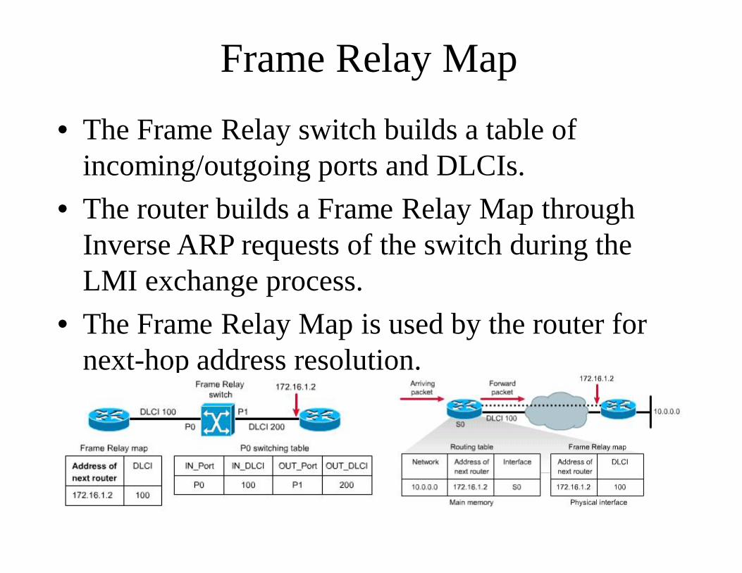
Frame Relay Map• The Frame Relay switch builds a table of
incoming/outgoing ports and DLCIs.• The router builds a Frame Relay Map through
Inverse ARP requests of the switch during the LMI exchange process.
• The Frame Relay Map is used by the router for next-hop address resolution.
Frame Relay-IARP
• FRADs know DLCIs of available PVCs (through LMI), but don’t know IP addresses of other ends
• IP addresses for given DLCIs are obtained automatically; mapping IP-DLCI is generated - dynamic mapping
• IARP can be switched of; static maps have to be generated by FRAD user
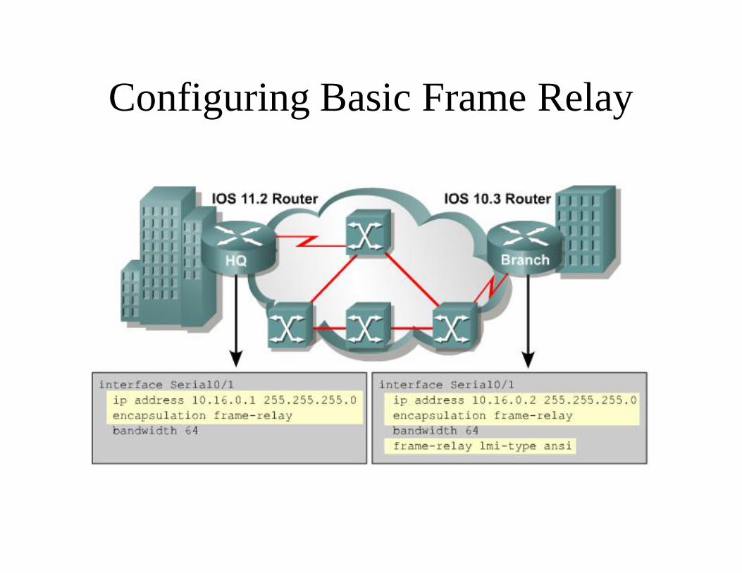
Configuring Basic Frame Relay
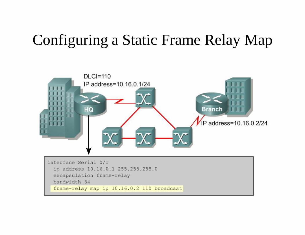
Configuring a Static Frame Relay Map
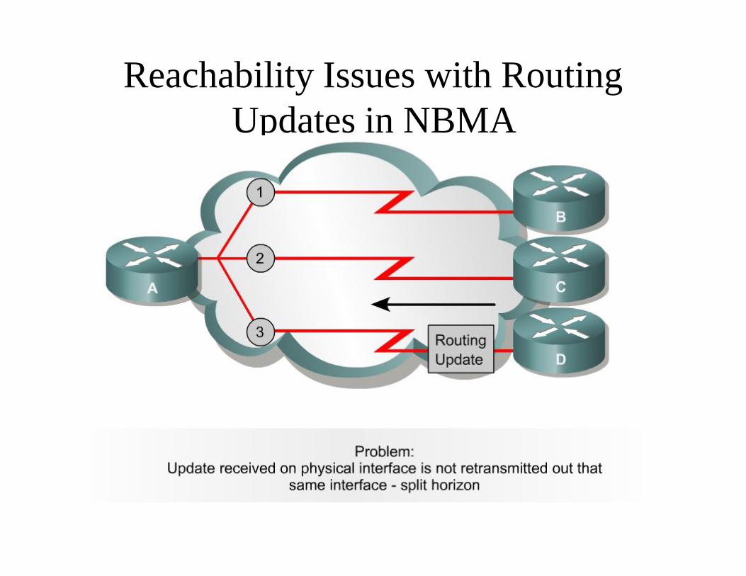
Reachability Issues with Routing Updates in NBMA
Reachability Issues with Routing Updates in NBMA
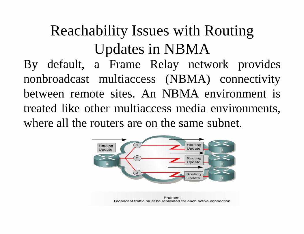
By default, a Frame Relay network providesnonbroadcast multiaccess (NBMA) connectivitybetween remote sites. An NBMA environment istreated like other multiaccess media environments,where all the routers are on the same subnet.
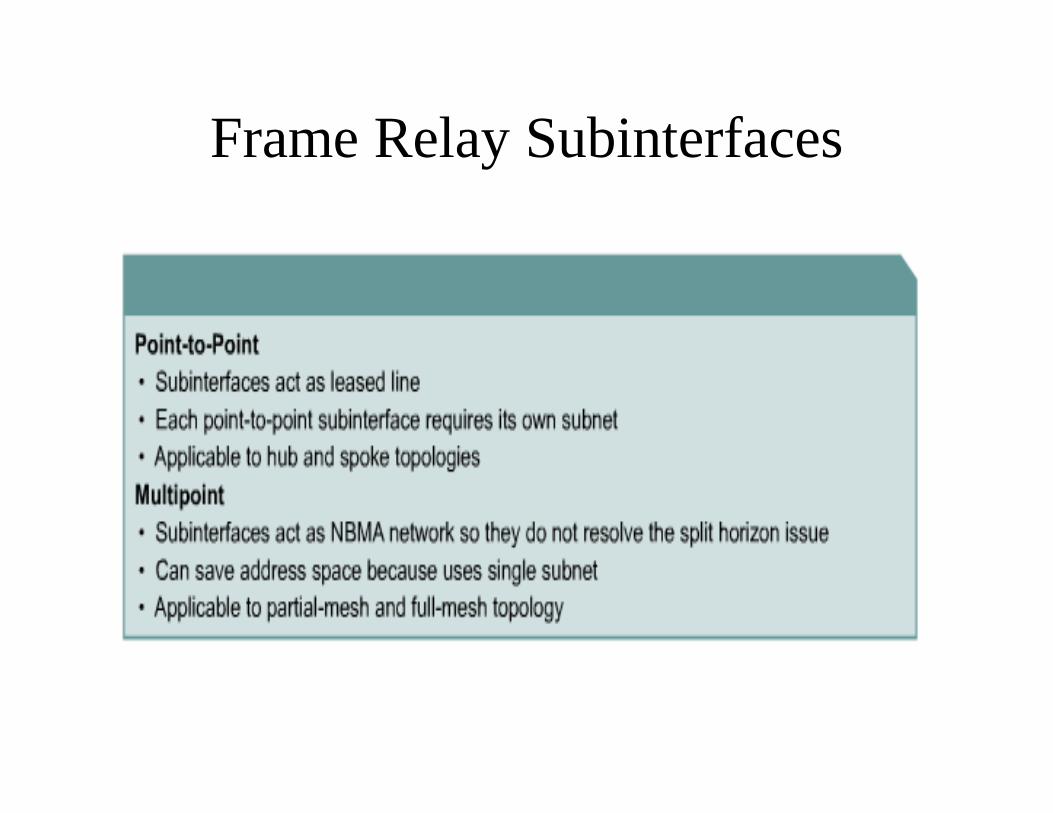
Frame Relay Subinterfaces
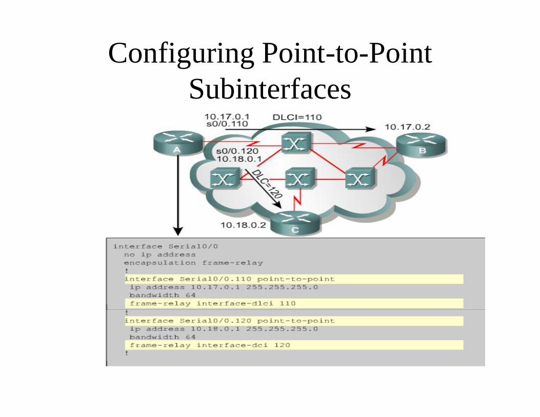
Configuring Point-to-Point Subinterfaces
Verifying Frame Relay
• The show interfaces command displays information regarding the encapsulation and Layer 1 and Layer 2 status. It also displays information about the following:
The LMI type The LMI DLCI The Frame Relay data terminal equipment/data circuit-terminating equipment (DTE/DCE) type

ATM
Broadband Integrated Services Networks
• In the mid-1980s, the ITU-T (formerly CCITT) initiated a standardization effort to merge voice, video and data on a single network
• The goal was to replace all existing networks (telephony networks, Cable TV network, data networks) with a single network infrastructure. The effort was called B-ISDN (Broadband Integrated Services Digital Networks)
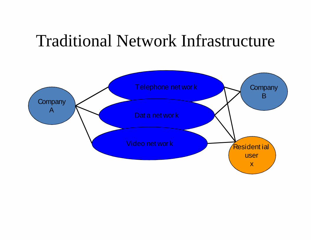
Traditional Network Infrastructure
CompanyA
CompanyB
Telephone network
Data network
Residential user
x
Video network
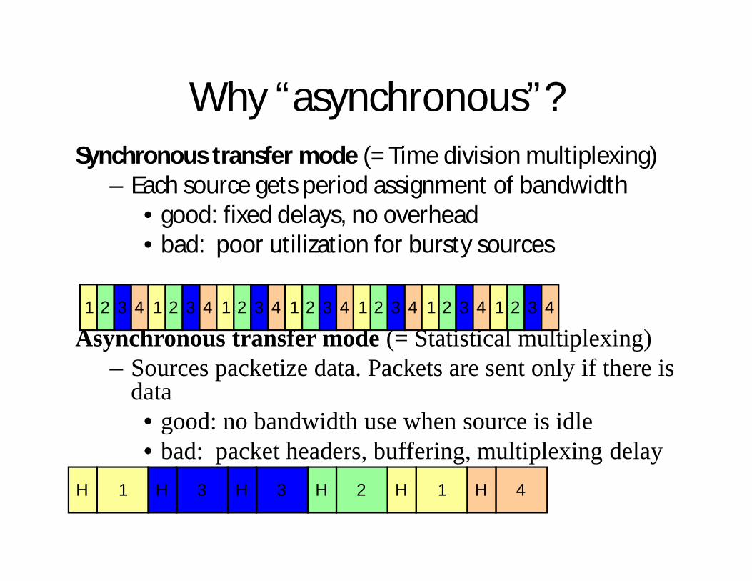
Why “asynchronous”? Synchronous transfer mode (= Time division multiplexing)
– Each source gets period assignment of bandwidth• good: fixed delays, no overhead• bad: poor utilization for bursty sources
Asynchronous transfer mode (= Statistical multiplexing) – Sources packetize data. Packets are sent only if there is
data• good: no bandwidth use when source is idle• bad: packet headers, buffering, multiplexing delay
1 2 3 4 1 2 3 4 1 2 3 4 1 2 3 4 1 2 3 4 1 2 3 4 1 2 3 4
1H 3H 3H 2H 1H 4H
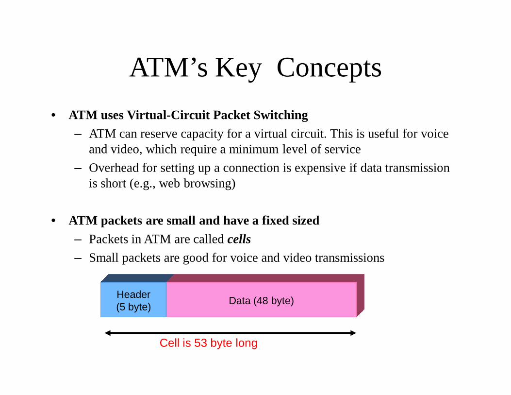
ATM’s Key Concepts • ATM uses Virtual-Circuit Packet Switching
– ATM can reserve capacity for a virtual circuit. This is useful for voice and video, which require a minimum level of service
– Overhead for setting up a connection is expensive if data transmission is short (e.g., web browsing)
• ATM packets are small and have a fixed sized – Packets in ATM are called cells– Small packets are good for voice and video transmissions
Header(5 byte) Data (48 byte)
Cell is 53 byte long
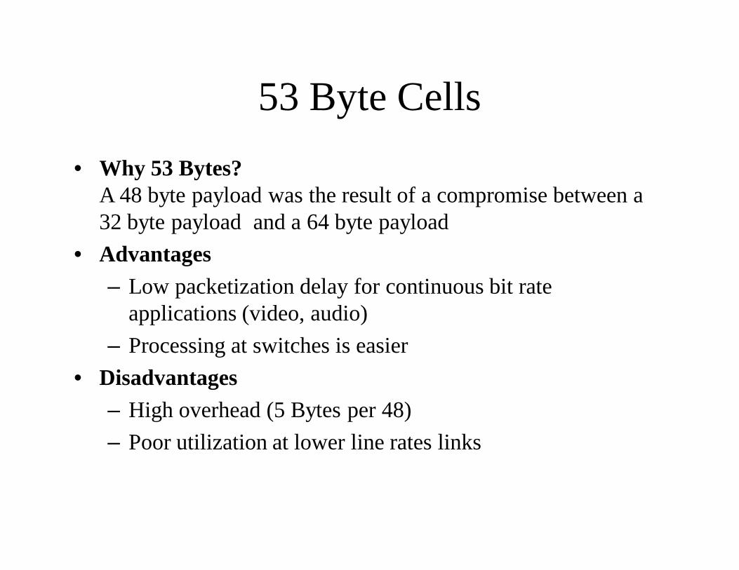
53 Byte Cells• Why 53 Bytes?
A 48 byte payload was the result of a compromise between a 32 byte payload and a 64 byte payload
• Advantages– Low packetization delay for continuous bit rate
applications (video, audio) – Processing at switches is easier
• Disadvantages– High overhead (5 Bytes per 48)– Poor utilization at lower line rates links
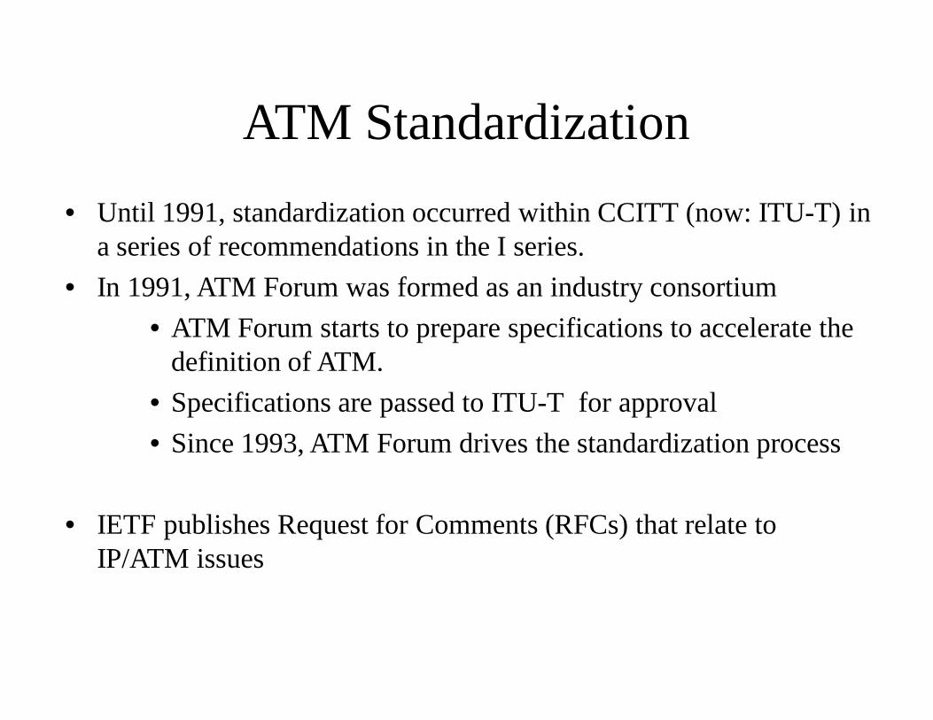
ATM Standardization• Until 1991, standardization occurred within CCITT (now: ITU-T) in
a series of recommendations in the I series.• In 1991, ATM Forum was formed as an industry consortium
• ATM Forum starts to prepare specifications to accelerate the definition of ATM.
• Specifications are passed to ITU-T for approval• Since 1993, ATM Forum drives the standardization process
• IETF publishes Request for Comments (RFCs) that relate to IP/ATM issues
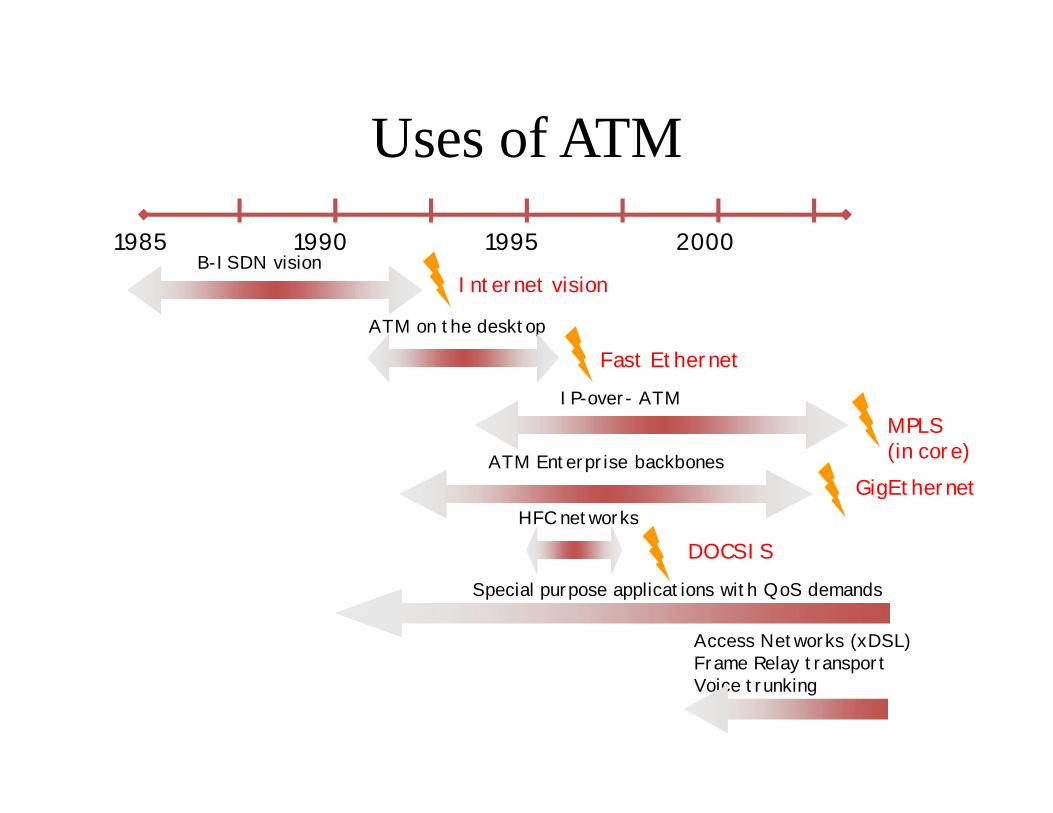
Uses of ATM1985 1990 1995 2000
B-ISDN vision
ATM on the desktop
IP-over- ATM
ATM Enterprise backbones
Fast Ethernet
MPLS (in core)
Internet vision
GigEthernet
Special purpose applications with QoS demands
Access Networks (xDSL)Frame Relay transport Voice trunking
DOCSISHFC networks
ATM ArchitectureOverview
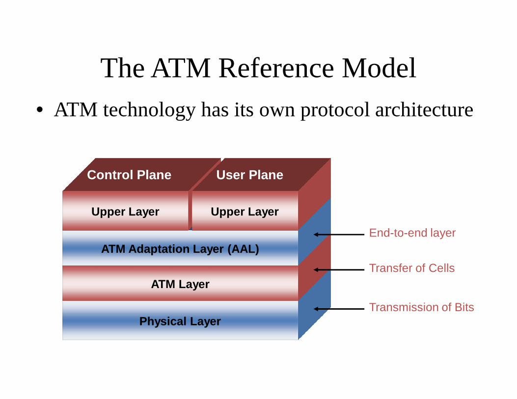
The ATM Reference Model• ATM technology has its own protocol architecture
Physical Layer
ATM Layer
ATM Adaptation Layer (AAL)
Upper Layer Upper Layer
Control Plane User Plane
Transmission of Bits
Transfer of Cells
End-to-end layer
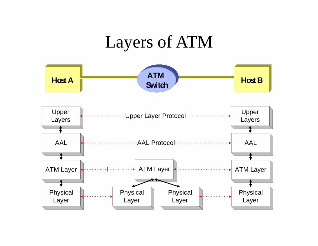
Layers of ATM
AAL
ATM Layer
PhysicalLayer
PhysicalLayer
PhysicalLayer
ATM Layer
AAL
ATM Layer
PhysicalLayer
AAL Protocol
l
UpperLayers
UpperLayersUpper Layer Protocol
Host AATM Switch
Host B
ATM Layer
• The ATM Layer is responsible for the transport of 53 byte cells across an ATM network
• Multiplex logical channels within a physical channel
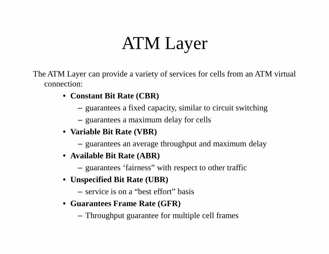
ATM LayerThe ATM Layer can provide a variety of services for cells from an ATM virtual
connection:• Constant Bit Rate (CBR)
– guarantees a fixed capacity, similar to circuit switching– guarantees a maximum delay for cells
• Variable Bit Rate (VBR)– guarantees an average throughput and maximum delay
• Available Bit Rate (ABR)– guarantees ‘fairness” with respect to other traffic
• Unspecified Bit Rate (UBR)– service is on a “best effort” basis
• Guarantees Frame Rate (GFR)– Throughput guarantee for multiple cell frames
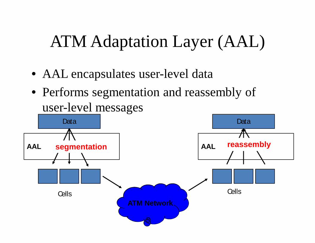
ATM Adaptation Layer (AAL)
• AAL encapsulates user-level data• Performs segmentation and reassembly of
user-level messagesData
AAL
Data
AAL
Cells Cells
ATM Network
segmentation reassembly

ATM Cells
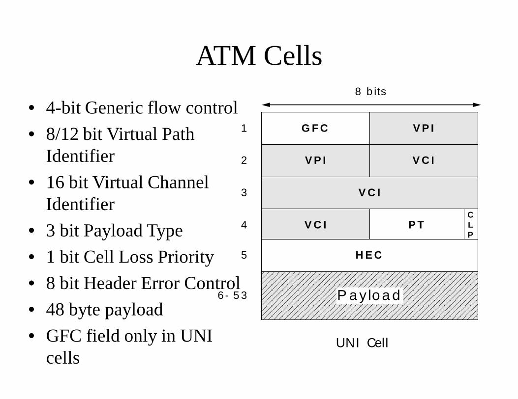
ATM Cells
• 4-bit Generic flow control • 8/12 bit Virtual Path
Identifier• 16 bit Virtual Channel
Identifier• 3 bit Payload Type• 1 bit Cell Loss Priority• 8 bit Header Error Control• 48 byte payload• GFC field only in UNI
cells
V C I
8 b its
G F C V P I
V P I V C I
V C I P TCLP
H E C
1
2
3
4
5
P a ylo a d6 - 5 3
UNI Cell
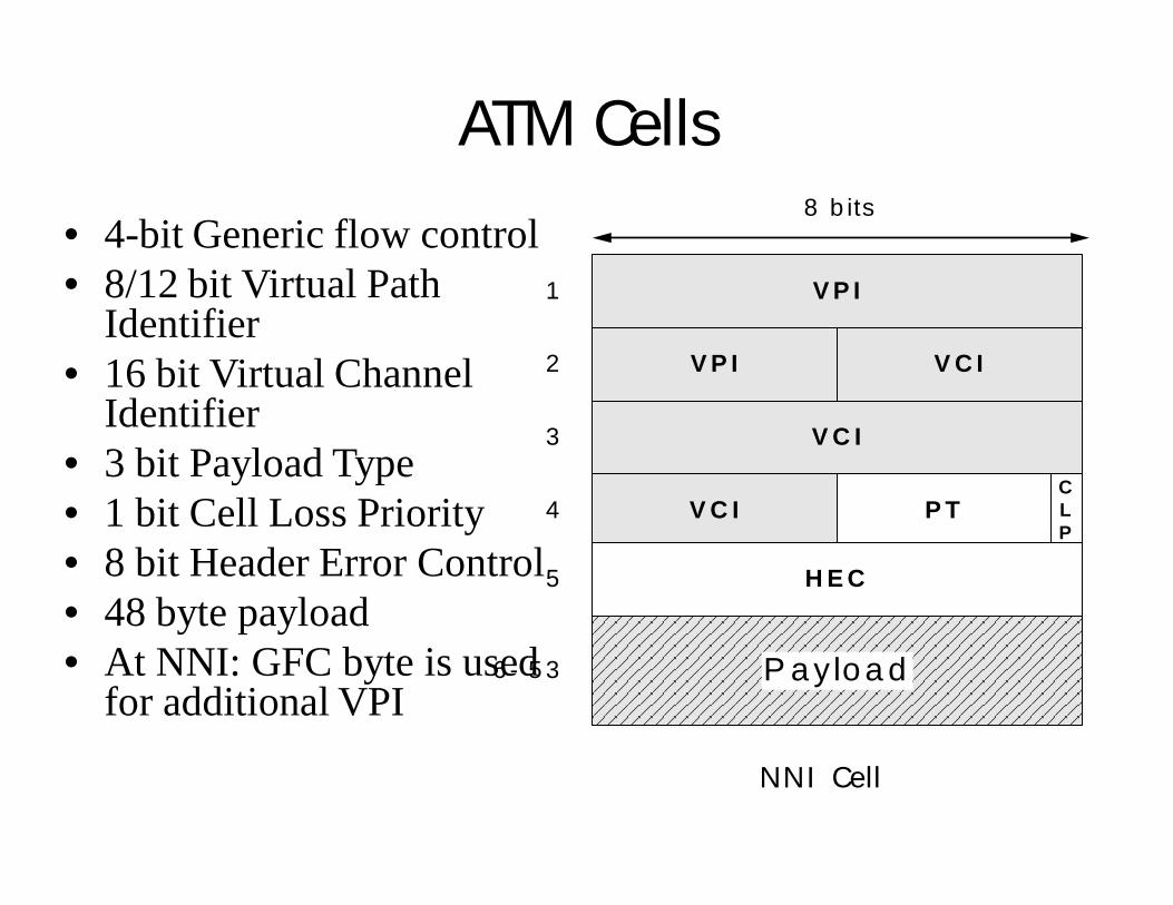
ATM Cells• 4-bit Generic flow control • 8/12 bit Virtual Path
Identifier• 16 bit Virtual Channel
Identifier• 3 bit Payload Type• 1 bit Cell Loss Priority• 8 bit Header Error Control• 48 byte payload• At NNI: GFC byte is used
for additional VPI
V C I
8 b its
V P I V C I
V C I P TCLP
H E C
1
2
3
4
5
P a ylo a d6 - 5 3
V P I
NNI Cell
ATM Connections
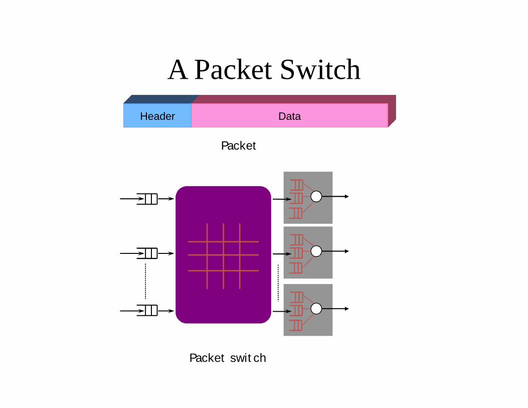
A Packet SwitchHeader Data
Packet switch
Packet
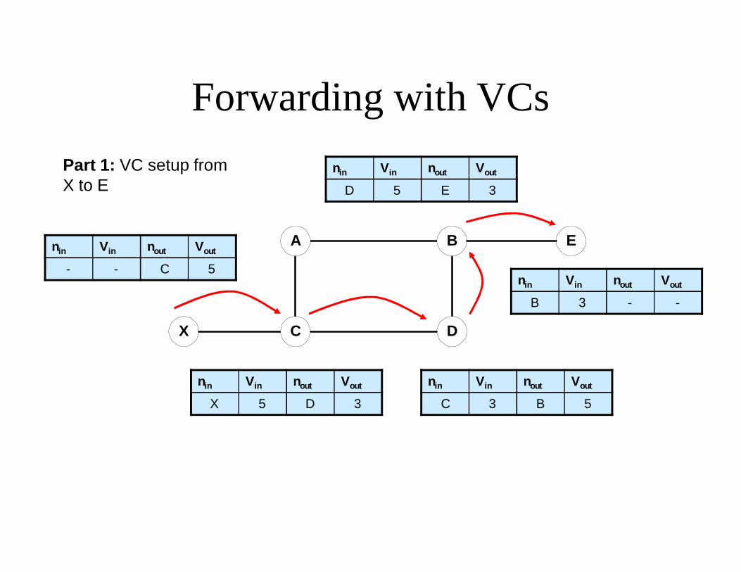
Forwarding with VCs
X
EA
C
B
D
nin Vin nout Vout
- - C 5
nin Vin nout Vout
X 5 D 3nin Vin nout Vout
C 3 B 5
nin Vin nout Vout
D 5 E 3
nin Vin nout Vout
B 3 - -
Part 1: VC setup from X to E
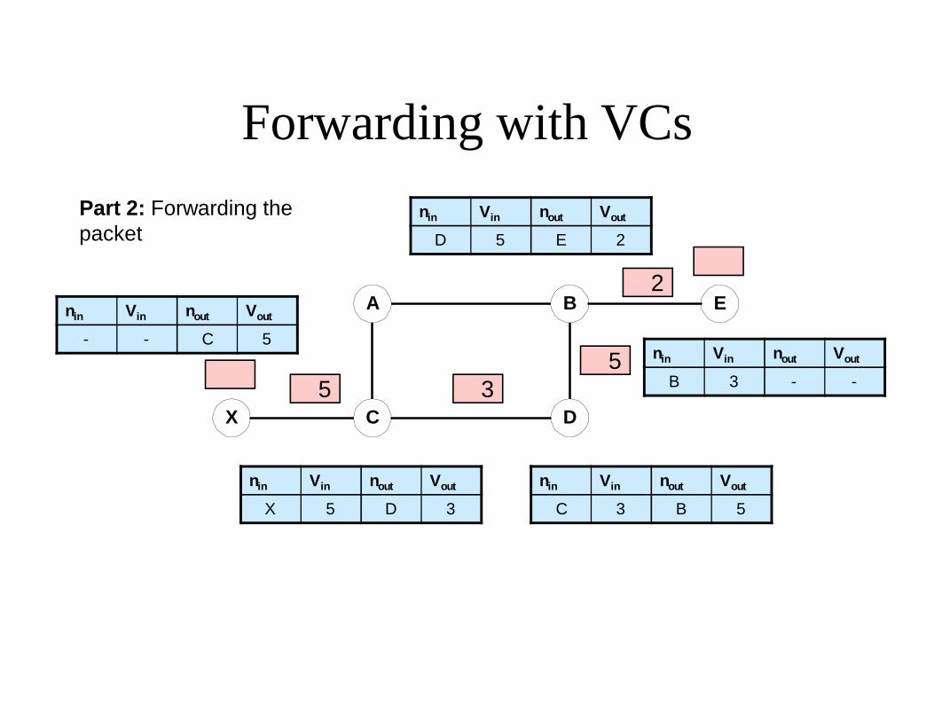
Forwarding with VCs
X
EA
C
B
D
nin Vin nout Vout
- - C 5
nin Vin nout Vout
X 5 D 3nin Vin nout Vout
C 3 B 5
nin Vin nout Vout
D 5 E 2
nin Vin nout Vout
B 3 - -55
3
2
Part 2: Forwarding the packet
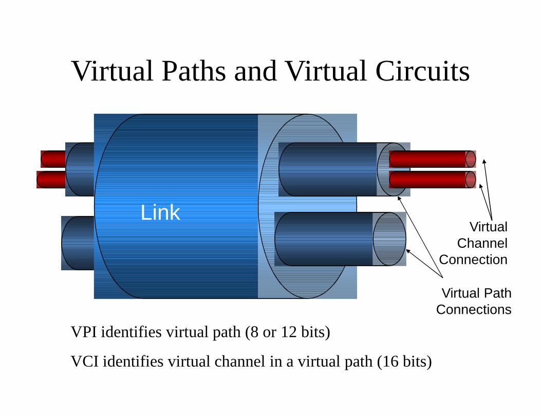
Virtual Paths and Virtual Circuits
Virtual Path Connections
Virtual Channel
Connection
VPI identifies virtual path (8 or 12 bits)
VCI identifies virtual channel in a virtual path (16 bits)
Link
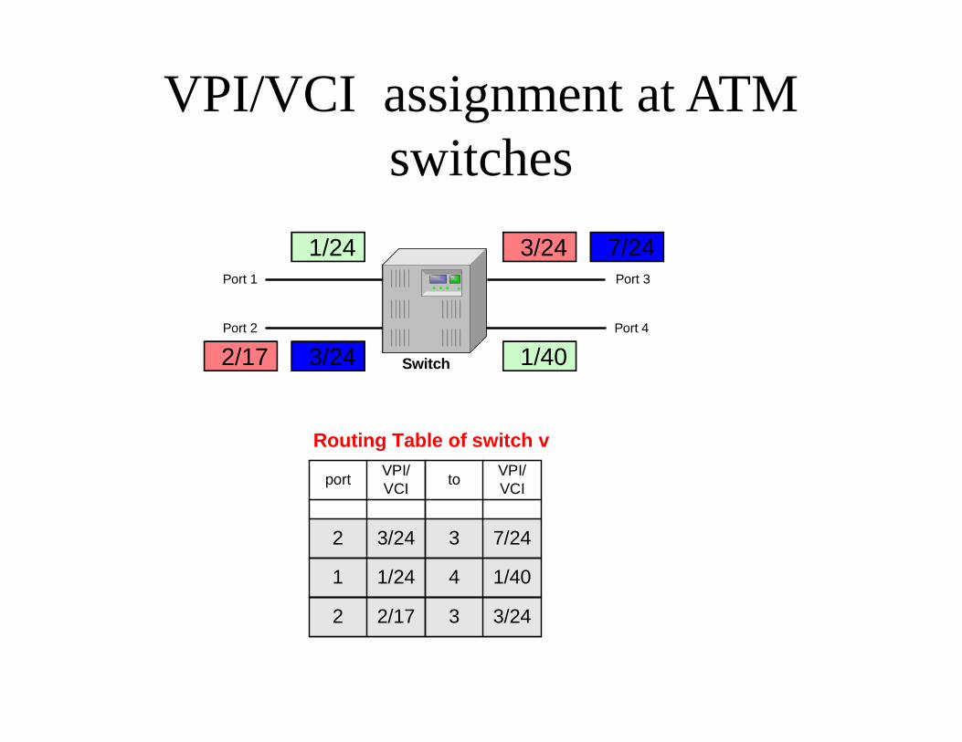
3/2432/172
7/2433/242
1/4041/241
Routing Table of switch v
port VPI/VCI to VPI/
VCI
Port 1
Port 2
Port 3
Port 4
Switch
VPI/VCI assignment at ATM switches
1/24 7/24
3/24 1/40
3/24
2/17
Addressing and Signaling
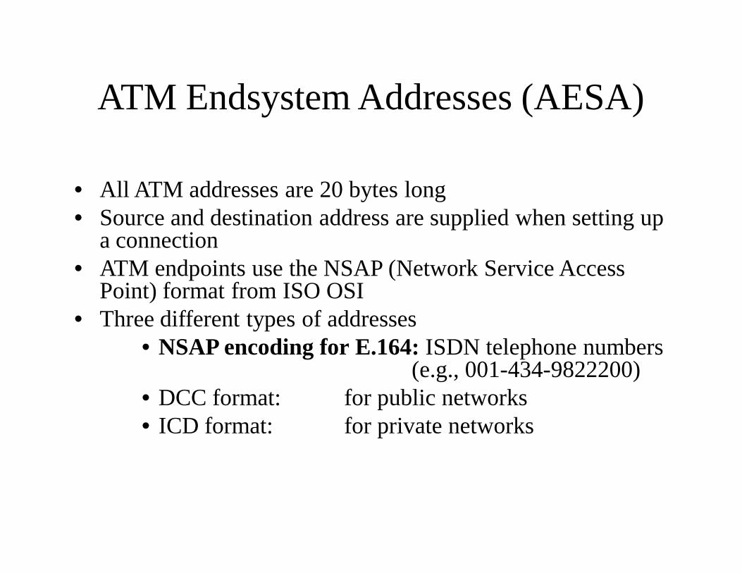
ATM Endsystem Addresses (AESA)
• All ATM addresses are 20 bytes long• Source and destination address are supplied when setting up
a connection• ATM endpoints use the NSAP (Network Service Access
Point) format from ISO OSI• Three different types of addresses
• NSAP encoding for E.164: ISDN telephone numbers (e.g., 001-434-9822200)
• DCC format: for public networks• ICD format: for private networks
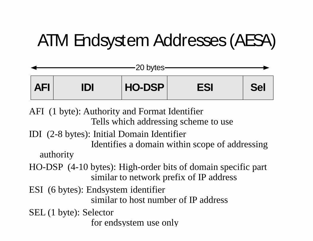
ATM Endsystem Addresses (AESA)
AFI (1 byte): Authority and Format IdentifierTells which addressing scheme to use
IDI (2-8 bytes): Initial Domain IdentifierIdentifies a domain within scope of addressing
authorityHO-DSP (4-10 bytes): High-order bits of domain specific part
similar to network prefix of IP addressESI (6 bytes): Endsystem identifier
similar to host number of IP addressSEL (1 byte): Selector
for endsystem use only
AFI
20 bytes
IDI HO-DSP ESI Sel
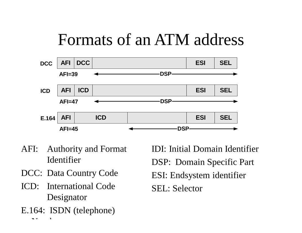
Formats of an ATM address
AFI: Authority and Format Identifier
DCC: Data Country CodeICD: International Code
DesignatorE.164: ISDN (telephone)
Number
DSP
AFI DCC ESI SELDCC
AFI=39
DSP
AFI ICD ESI SELICD
AFI=47
DSP
AFI ICD ESI SELE.164
AFI=45
IDI: Initial Domain IdentifierDSP: Domain Specific PartESI: Endsystem identifierSEL: Selector
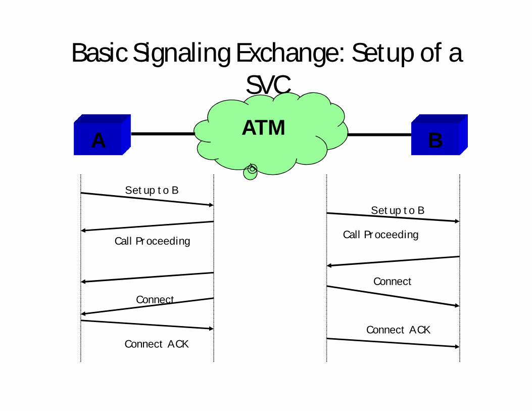
Basic Signaling Exchange: Setup of a SVC
A
Setup to B
Call Proceeding
Setup to B
ConnectConnect
Connect ACKConnect ACK
BATM
Call Proceeding
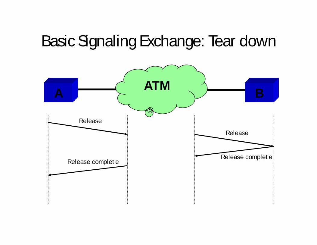
Release
Release
Release completeRelease complete
Basic Signaling Exchange: Tear down
A BATM

ATM Layer Services
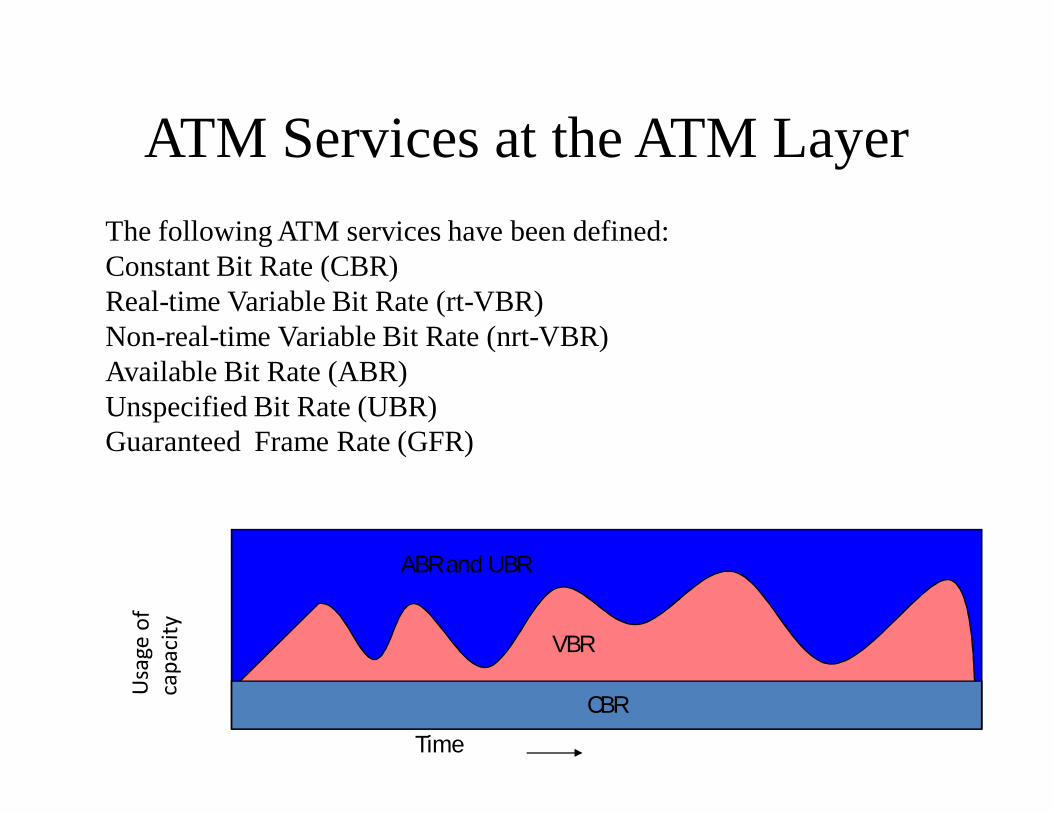
ATM Services at the ATM LayerThe following ATM services have been defined:Constant Bit Rate (CBR)Real-time Variable Bit Rate (rt-VBR)Non-real-time Variable Bit Rate (nrt-VBR)Available Bit Rate (ABR) Unspecified Bit Rate (UBR)Guaranteed Frame Rate (GFR)
Time
CBR
VBR
ABR and UBR
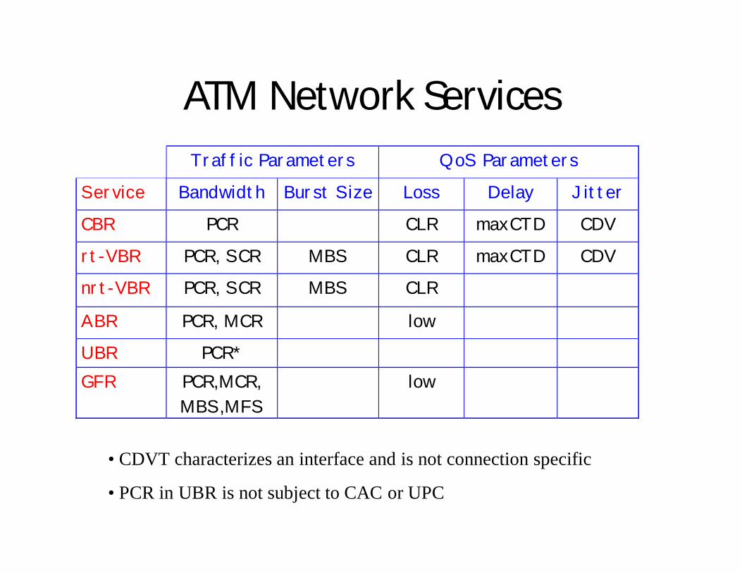
ATM Network Services Traffic Parameters QoS Parameters
Service Bandwidth Burst Size Loss Delay Jitter
CBR PCR CLR maxCTD CDV
rt-VBR PCR, SCR MBS CLR maxCTD CDV
nrt-VBR PCR, SCR MBS CLR
ABR PCR, MCR low
UBR PCR* GFR PCR,MCR,
MBS,MFS low
• CDVT characterizes an interface and is not connection specific
• PCR in UBR is not subject to CAC or UPC
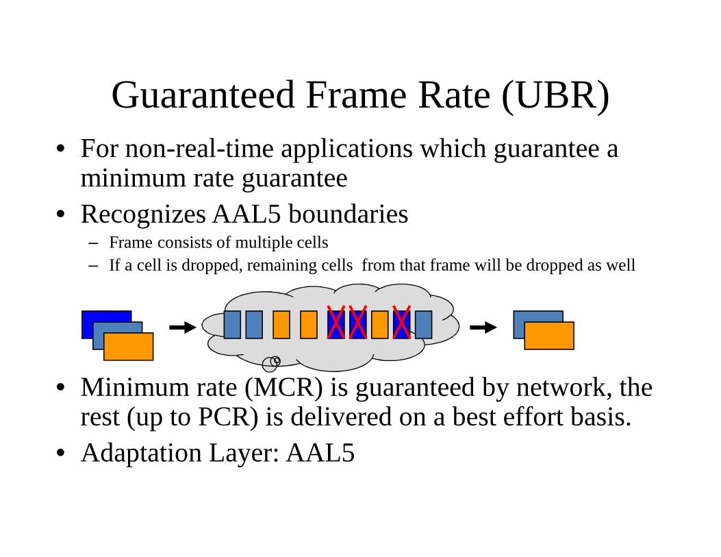
Guaranteed Frame Rate (UBR)• For non-real-time applications which guarantee a
minimum rate guarantee • Recognizes AAL5 boundaries
– Frame consists of multiple cells– If a cell is dropped, remaining cells from that frame will be dropped as well
• Minimum rate (MCR) is guaranteed by network, the rest (up to PCR) is delivered on a best effort basis.
• Adaptation Layer: AAL5
UNIT IV NETWORK TRAFFIC MANAGEMENT
ATM Traffic and congestion control
Why Traffic Management?• The ATM technology is intended to support a wide variety of
services and applications such as voice, video, and data• ATM promises to support all these different requirements with
a common network• Within such a network all connections may impact on each
other• ATM must manage traffic fairly and provide effective
allocation of network resources for these different applications • It is the task of ATM traffic control to:
– protect the network and the end-systems from congestion in order to provide specified and guaranteed levels of Quality of Service (QoS)
– use available network resources efficiently
Network Congestion• Network congestion is a state when the network cannot meet
the negotiated network performance objectives for established connections or for new connection requests
• Network congestion can be caused by:– Unpredictable statistical fluctuation of traffic flows– Fault conditions within the network
• ATM layer traffic control is a set of actions taken by the network to avoid network congestion
• Traffic control takes measures to adapt to unpredictable fluctuations in traffic flows and other problems within the network.
• ATM layer congestion control refers to the set of actions taken by the network to minimize the intensity, spread, and duration of congestion
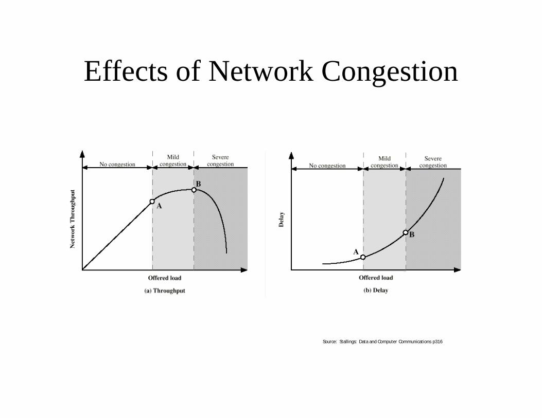
Effects of Network Congestion
Source: Stallings: Data and Computer Communications p316
Traffic Parameters• Traffic parameters describe traffic characteristics of a
connection• For a given connection, traffic parameters are grouped into a
source traffic descriptor• Traffic parameters specified in ATM Forum UNI
– Peak Cell Rate (PCR)• An upper bound on the rate that traffic can be submit on
a connection• Measured in cells/second
– Sustainable Cell Rate (SCR)• An upper bound on the average cell rate of a burst
traffic of an ATM connection • Measured in cells/second
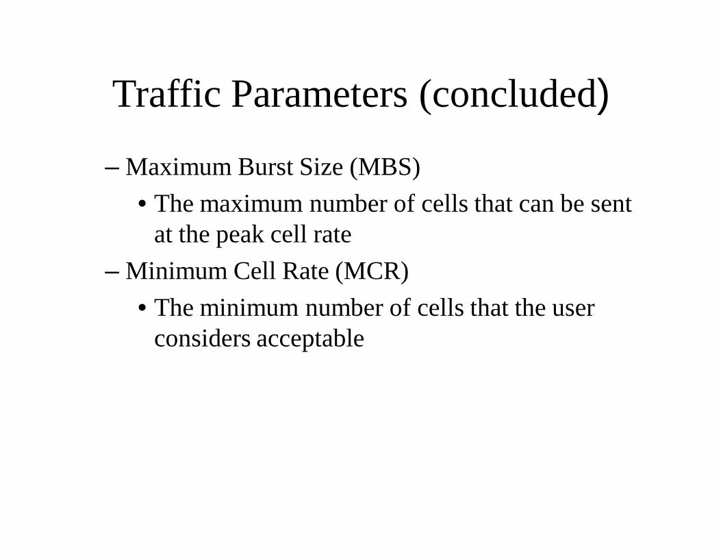
Traffic Parameters (concluded)
– Maximum Burst Size (MBS)• The maximum number of cells that can be sent
at the peak cell rate– Minimum Cell Rate (MCR)
• The minimum number of cells that the user considers acceptable
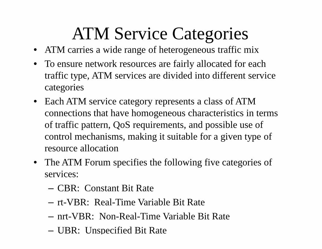
ATM Service Categories• ATM carries a wide range of heterogeneous traffic mix• To ensure network resources are fairly allocated for each
traffic type, ATM services are divided into different service categories
• Each ATM service category represents a class of ATM connections that have homogeneous characteristics in terms of traffic pattern, QoS requirements, and possible use of control mechanisms, making it suitable for a given type of resource allocation
• The ATM Forum specifies the following five categories of services:– CBR: Constant Bit Rate– rt-VBR: Real-Time Variable Bit Rate– nrt-VBR: Non-Real-Time Variable Bit Rate– UBR: Unspecified Bit Rate
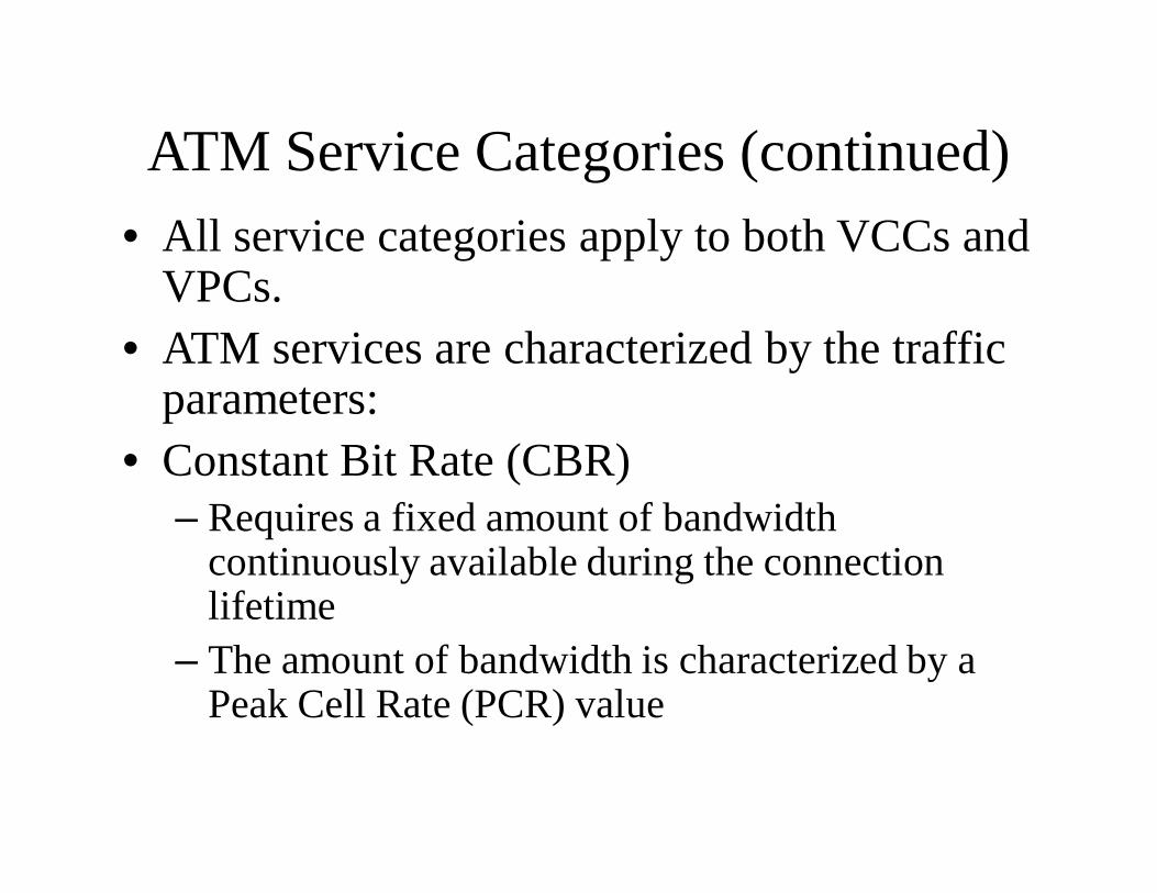
ATM Service Categories (continued)• All service categories apply to both VCCs and
VPCs.• ATM services are characterized by the traffic
parameters:• Constant Bit Rate (CBR)
– Requires a fixed amount of bandwidth continuously available during the connection lifetime
– The amount of bandwidth is characterized by a Peak Cell Rate (PCR) value
ATM Service Categories (continued)
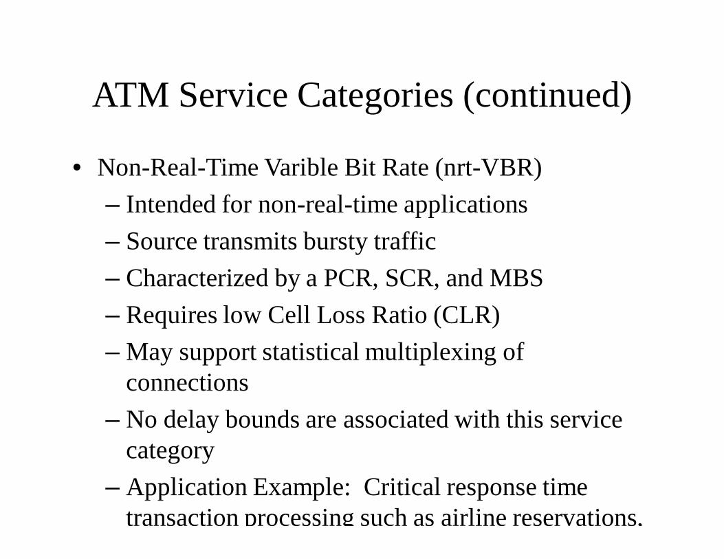
• Non-Real-Time Varible Bit Rate (nrt-VBR)– Intended for non-real-time applications– Source transmits bursty traffic– Characterized by a PCR, SCR, and MBS– Requires low Cell Loss Ratio (CLR)– May support statistical multiplexing of
connections– No delay bounds are associated with this service
category– Application Example: Critical response time
transaction processing such as airline reservations,
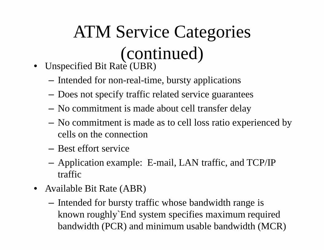
ATM Service Categories (continued)
• Unspecified Bit Rate (UBR)– Intended for non-real-time, bursty applications– Does not specify traffic related service guarantees– No commitment is made about cell transfer delay– No commitment is made as to cell loss ratio experienced by
cells on the connection– Best effort service– Application example: E-mail, LAN traffic, and TCP/IP
traffic• Available Bit Rate (ABR)
– Intended for bursty traffic whose bandwidth range is known roughly`End system specifies maximum required bandwidth (PCR) and minimum usable bandwidth (MCR)
Quality of Service (QoS)• QoS is a set of user-perceivable performance
parameters that characterize the traffic over an ATM connection
• Defined on an end-to-end basis• User requests a QoS class for an ATM connection• The requested QoS class is a part of the traffic
contract• The network commits to meet the requested QoS as
long as the user complies with the traffic contract• ATM Forum QoS Classes
Quality of Service (QoS) Parameters
• QoS parameters describe the level of service for each connection
• ATM Forum specified six QoS parameters• Through the use of network signaling to establish an
ATM connection, three of these may be negotiated between the end-system and the network– Peak-to-peak Cell Delay Variation (peak-to-peak
CDV)– Maximum Cell Transfer Delay (maxCTD)– Cell Loss Ratio (CLR)
Quality of Service (QoS) Parameters (continued)
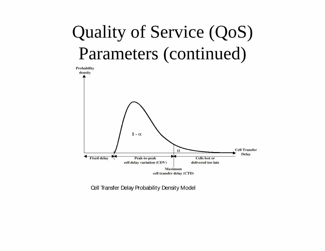
Cell Transfer Delay Probability Density Model
Quality of Service (QoS) Parameters (concluded)
• Higher values of cell loss is dominated by the effects of queuing strategy and buffer sizes
• Delay, delay variation, and cell loss are impacted by buffer size and buffering strategy
• The error rate is determined by fiber transmission characteristics
Traffic Contract• Agreement between user and network across UNI regarding:
– The QoS that a network is expected to provide– The Connection Traffic Descriptor, which includes
• Source Traffic Descriptor• Cell Delay Variation Tolerance (CDVT)• Conformance Definition
– Source Traffic Descriptor• Defines the characteristics of ATM traffic coming into
the network • Includes several negotiable traffic parameters: PCR,
SCR, MBS, and Burst Tolerance (BT)• Specifies flow for CLP = 0 and/or CLP = 0 + 1
– Cell Delay Variation Tolerance (CDVT)
Traffic Contract (concluded)
• A separate traffic contract for each Virtual Path Connection (VPC) or Virtual Channel Connection (VCC)
• Negotiated at connection time– Signaling message for SVC– Circuit provision for PVC
Traffic Control Functions
• Connection Admission Control (CAC)• Usage Parameter Control (UPC)• Selective cell discarding• Traffic Shaping• Explicit Forward Congestion Indication (EFCI)• Cell Loss Priority Control• Network Resource Management (NRM)• Frame discard• ABR Flow Control• Others
Selective Cell Discard and EFCI• Selective Cell discard
– A congested network may selectively discard cells which meet either or both the following conditions:
• Cells which belong to a non-compliant ATM connection• Cells which have CLP = 1
– This is to protect the CLP = 0 flow as much as possible• Explicit Forward congestion Indication (EFCI)
– A network element in an impending congested state or a congested state may set an EFCI in the cell header
– This indication may be examined by the destination end-system
– The end-system may adaptively lower the cell rate of the connection
Traffic Shaping
• A mechanism that alters the traffic characteristics of a cell stream on a connection to achieve better network efficiency or to ensure conformance to the traffic parameters in the traffic contract
• Traffic shaping examples:– Peak cell rate reduction– Burst length limiting– Spacing cells in time to reduce CDV– Cell scheduling policy
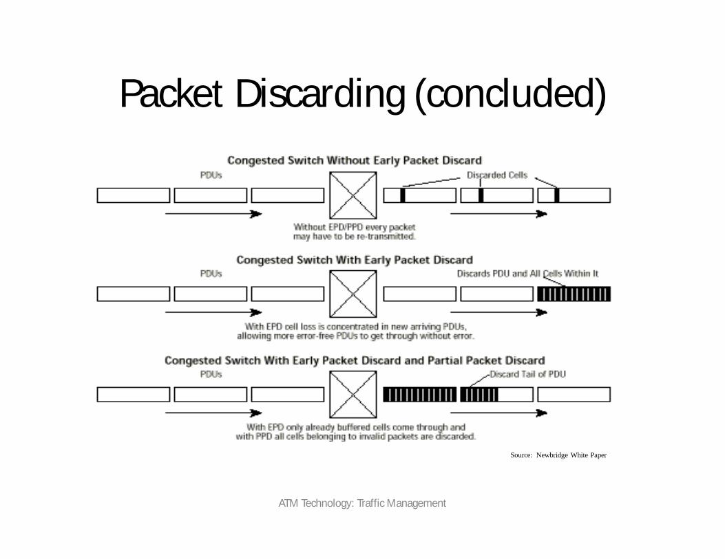
Packet Discarding• The ATM Adaptation Layer (AAL) segments higher layer
packets into small fixed-size cells for transporting over the ATM network
• A cell discarded by a switch causes the loss of the entire packet and eventually requires end-to-end error recovery through packet retransmission
• A small congestion problem could potentially escalate to a more serious one
• To prevent congestion escalation, Early Packet Discard (EPD) and Partial Packet Discard (PPD) can be used to discard cells on a packet basis
• EPD and PPD are applied for ABR and UBR traffic of AAL-5 connections
Packet Discarding (continued)– The remaining buffer space can then be used for cells
belonging to packets that already have entered the queue
– EPD maximizes the chances for already queued packets to leave the queue successfully
• PPD– If EPD does not remove congestion and cells arriving
at a queue have to be discarded because of buffer overflow PPD is applied
– PPD discards all subsequent cells associated with the same packet rather than just a few cells within the packet during buffer overflow
ATM Technology: Traffic Management
Packet Discarding (concluded)
Source: Newbridge White Paper
• Traffic Management Roles:– Maximize efficiency– Minimize data loss– Control traffic during times of heavy
utilization• Control is based on:
– Connection Admission Control (CAC)– Call Routing– Network Resource Allocation
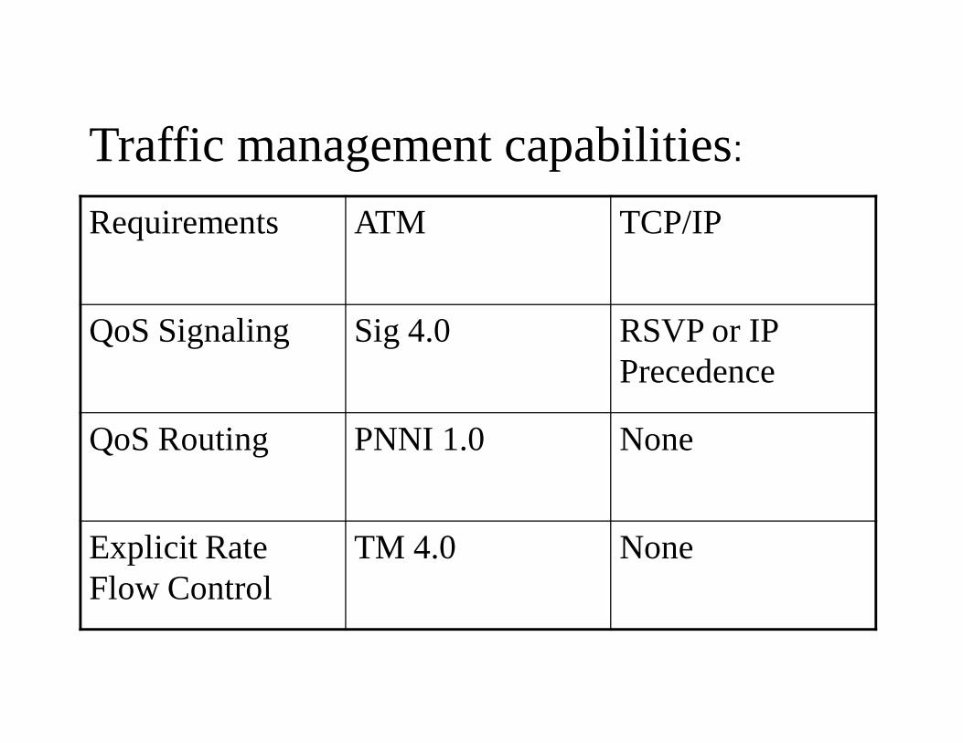
Traffic management capabilities:
Requirements ATM TCP/IP
QoS Signaling Sig 4.0 RSVP or IP Precedence
QoS Routing PNNI 1.0 None
Explicit Rate Flow Control
TM 4.0 None
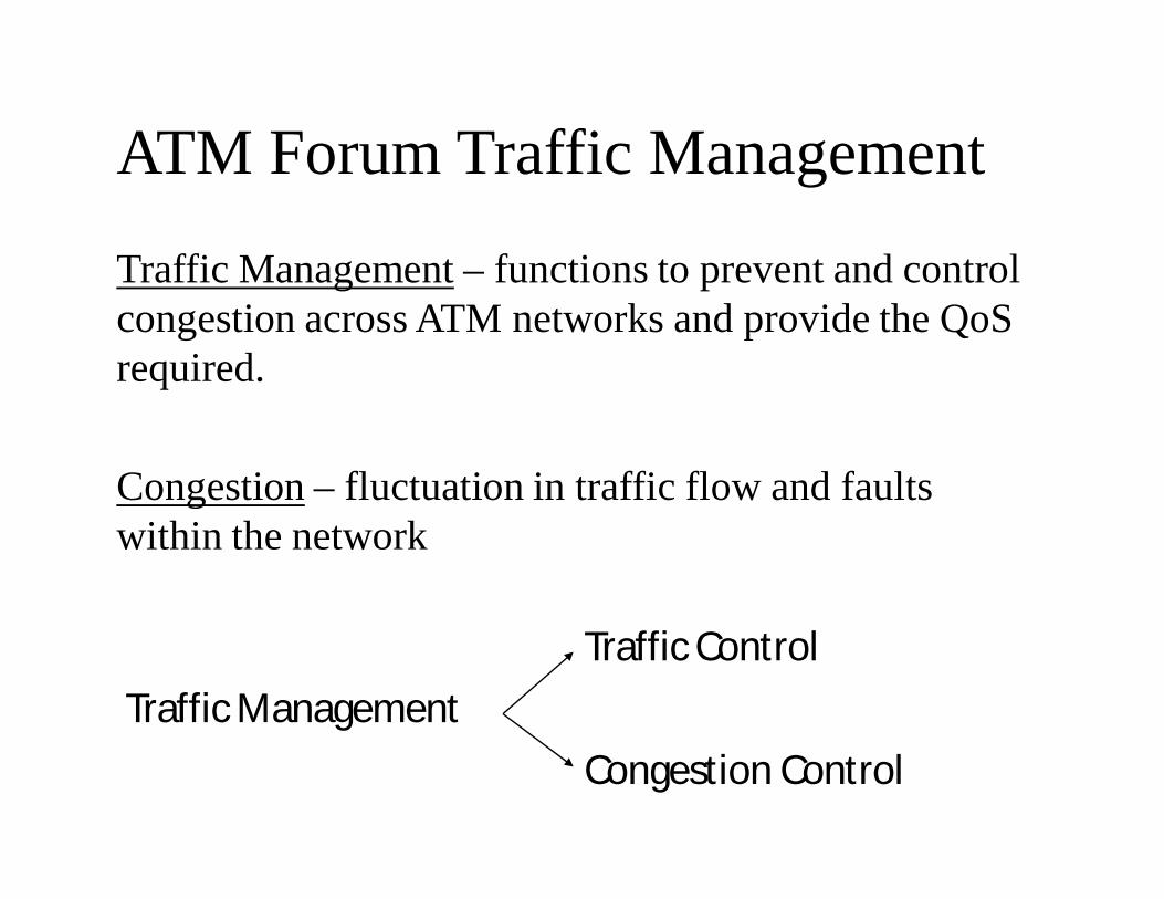
ATM Forum Traffic Management
Traffic Management – functions to prevent and control congestion across ATM networks and provide the QoSrequired.
Congestion – fluctuation in traffic flow and faults within the network
Traffic ManagementTraffic Control
Congestion Control
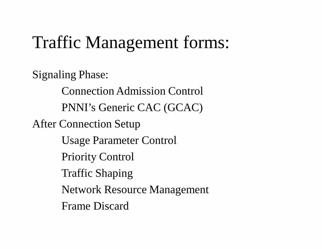
Traffic Management forms:
Signaling Phase:Connection Admission ControlPNNI’s Generic CAC (GCAC)
After Connection SetupUsage Parameter ControlPriority ControlTraffic ShapingNetwork Resource ManagementFrame Discard
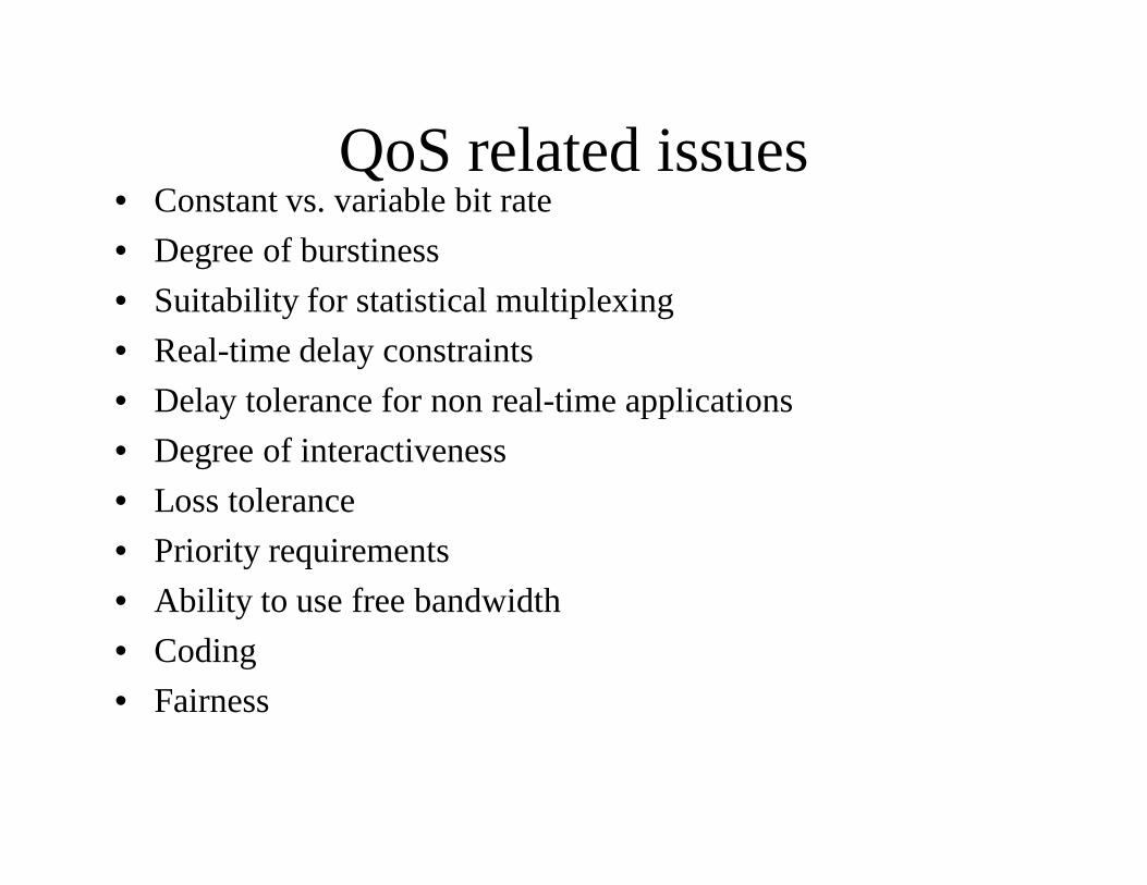
QoS related issues • Constant vs. variable bit rate• Degree of burstiness• Suitability for statistical multiplexing• Real-time delay constraints• Delay tolerance for non real-time applications• Degree of interactiveness• Loss tolerance• Priority requirements• Ability to use free bandwidth• Coding• Fairness

ATM Forum service categories:• Constant Bit Rate (CBR)• Real-time and non-real-time Variable Bit Rate (rt-
VBR nrt-VBR)• Unspecified Bit Rate (UBR)• Available Bit Rate (ABR)QoS Parameters:• Peak-to-peak Cell Delay Variation (ppCDV)• Maximum Cell Transfer Delay(Max CTD)• Mean Cell Transfer Delay (Mean CTD)• Cell Loss Ratio (CLR)
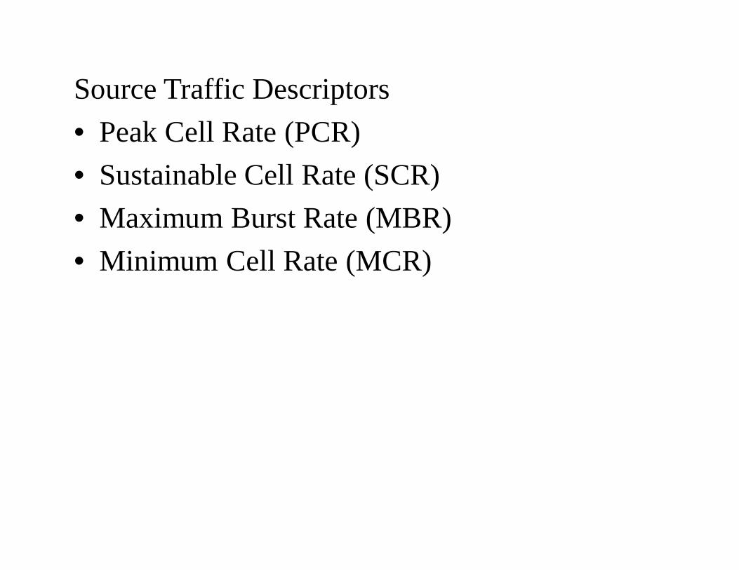
Source Traffic Descriptors• Peak Cell Rate (PCR)• Sustainable Cell Rate (SCR)• Maximum Burst Rate (MBR)• Minimum Cell Rate (MCR)
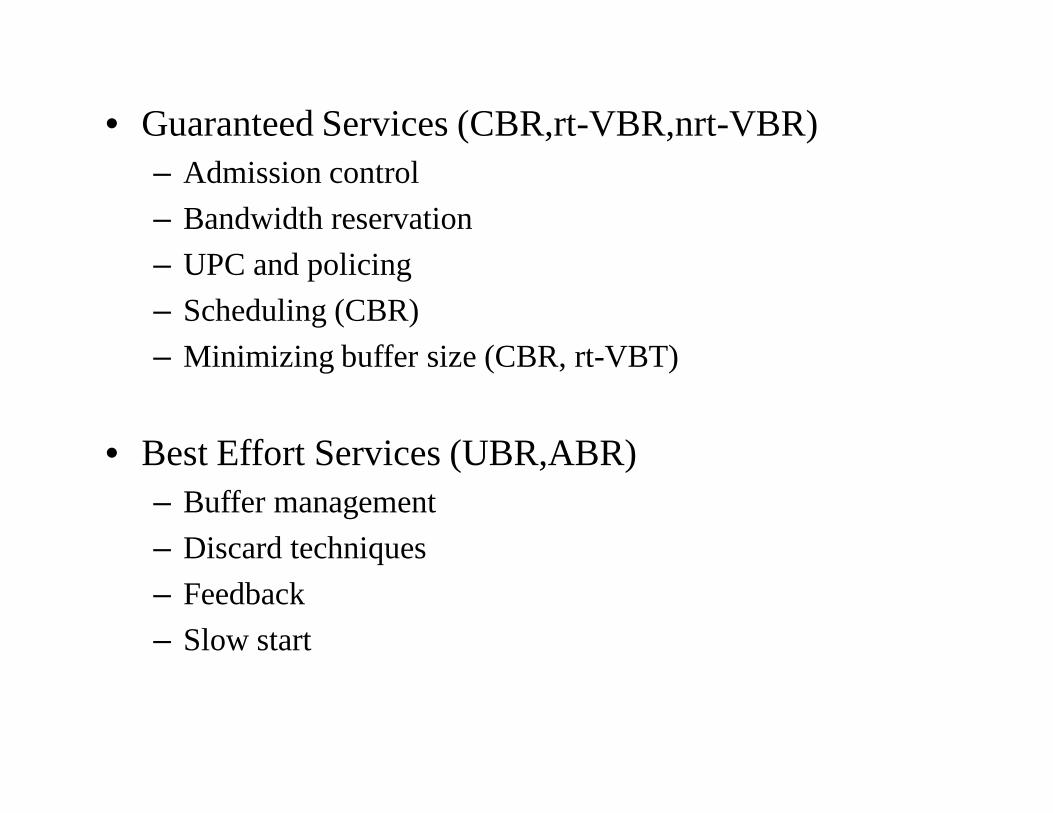
• Guaranteed Services (CBR,rt-VBR,nrt-VBR)– Admission control– Bandwidth reservation – UPC and policing– Scheduling (CBR)– Minimizing buffer size (CBR, rt-VBT)
• Best Effort Services (UBR,ABR)– Buffer management– Discard techniques– Feedback– Slow start
ABR
ABR
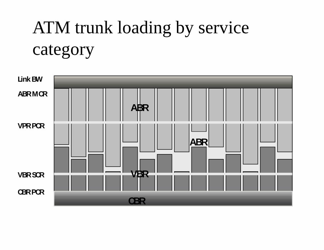
Link BW
ATM trunk loading by service category
CBR PCRCBR
CBR
VBR SCR
ABR MCR
VPR PCR
VBR
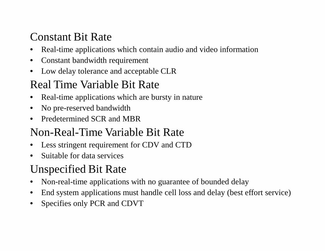
Constant Bit Rate• Real-time applications which contain audio and video information• Constant bandwidth requirement• Low delay tolerance and acceptable CLR
Real Time Variable Bit Rate• Real-time applications which are bursty in nature• No pre-reserved bandwidth • Predetermined SCR and MBR
Non-Real-Time Variable Bit Rate• Less stringent requirement for CDV and CTD• Suitable for data services
Unspecified Bit Rate• Non-real-time applications with no guarantee of bounded delay• End system applications must handle cell loss and delay (best effort service)• Specifies only PCR and CDVT
Available Bit Rate:• Sources which may vary in transmission rate but need service guarantees• Require low cell loss but allow for some delay• Can specify a minimal bandwidth
Traffic and Congestion Control Functions• Network Resource Management• Connection Admission Control• Usage Parameter Control• Selective Cell or Packet discarding• Traffic Shaping and Scheduling• Explicit Forward Congestion Indication• VP Resource Management• The ABR Mechnism
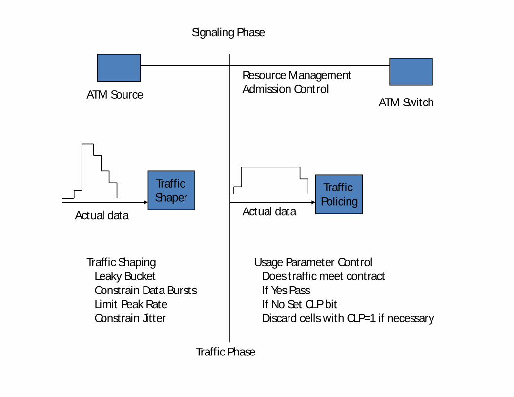
ATM Source
Signaling Phase
ATM Switch
Resource ManagementAdmission Control
Traffic Shaper
Actual data
Traffic Policing
Actual data
Traffic ShapingLeaky BucketConstrain Data BurstsLimit Peak RateConstrain Jitter
Traffic Phase
Usage Parameter ControlDoes traffic meet contractIf Yes PassIf No Set CLP bitDiscard cells with CLP=1 if necessary
Preventive Congestion Control• Leaky Bucket Algorithm – congestion control at the entry of
an ATM network• EFCI – feedback-based flow control• EPD and TPD – selective cell discarding
Reactive Congestion Control• Information propagates from ATM switches to ATM sources• Credit based or rate based• Rate based – uses bits in ATM header to inform the source
about the networks condition• Credit based – a form of windowing mechanism
ABR Service:• The source must adapt to network availability and limit it’s
output in order to receive an acceptable QoS• The source must specify a PCR and MCR• The network will divide the available network resources
among ABR connections
ABR: protocol operations• At setup the source specifies a number of parameters:
PCR,MCR, Initial Cell rate, Rate Increase Factor, Rate Decrease Factor, Transfer Buffer Exposure, Fixed Round Trip Time.
• The source sends RM cells in order to regulate it’s transmission rate
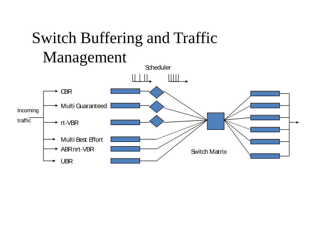
Switch Buffering and Traffic Management
Incoming
traffic
CBR
Multi Guaranteed
rt-VBR
Multi Best EffortABR nrt-VBR
UBR
Scheduler
Switch Matrix
Congestion: Effects
• Congestion is undesirable because it can cause:Increased delay, due to queueing within the networkPacket loss, due to buffer overflowReduced throughput, due to packet loss and retransmission
• Analogy: “rush hour” traffic
Congestion: Causes
• The basic cause of congestion is that the input traffic demands exceed the capacity of the network
• In typical packet switching networks, this can occur quite easily when:
- output links are slower than inputs- multiple traffic sources competing for same output link at the same time
Motivation
• The congestion control problem is even more acute in high speed networks
• Faster link speeds mean that congestion can happen faster than beforee.g., 64 kilobyte buffer
@ 64 kbps: 8.2 seconds@ 10 Mbps: 52 milliseconds@ 1 Gbps: 0.52 milliseconds
Reactive versus Preventive• There are two fundamental approaches to
congestion control: reactive approaches and preventive approaches
• Reactive: feedback-based– attempt to detect congestion, or the onset of
congestion, and take action to resolve the problem before things get worse
• Preventive: reservation-based– prevent congestion from ever happening in the
first place, by reserving resources
Reactive versus Preventive (Cont’d)• Most of the Internet approaches are reactive
schemes– TCP Slow Start– Random-Early-Detection (RED) Gateways– Source Quench
• The large d x b product means that many of these approaches are not applicable to high speed networks
• Most ATM congestion control strategies are preventive, reservation-based
Congestion Control in ATM
• When people discuss congestion control in the context of high speed ATM networks, they usually distinguish between call-level controls and cell-level controls
Call-Level Control
• An example of the call-level approach to congestion control is call admission control (to be discussed later this semester)
• Tries to prevent congestion by not allowing new calls or connections into the network unless the network has sufficient capacity to support them
Call-Level Control (Cont’d)
• At time of call setup (connection establishment) you request the resources that you need for the duration of the call (e.g., bandwidth, buffers)
• If available, your call proceeds• If not, your call is blocked• E.g., telephone network, busy signal
Call-Level Control (Cont’d)
• Tradeoff: aggressive vs conservative• Want to accept enough calls to have
reasonably high network utilization, but don’t want to accept so many calls that you have a high probability of network congestion (which might compromise the QOS requirements that you are trying to meet)
Cell-Level Control• Also called input rate control• Control the input rate of traffic sources to
prevent, reduce, or control the level of congestion
• Many possible mechanisms:Traffic shaping, traffic policing, UPCLeaky bucket (token bucket)Cell tagging (colouring), cell discardingCell scheduling disciplines
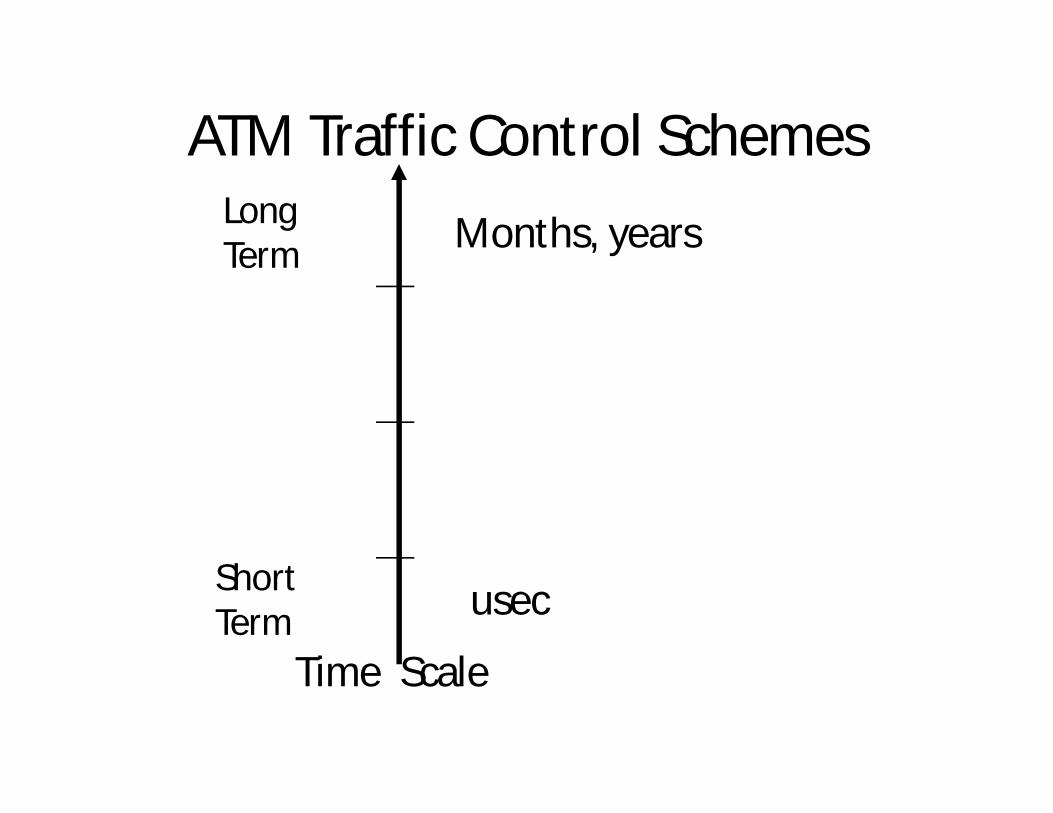
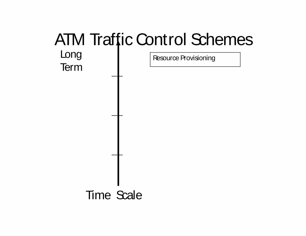
ATM Traffic Control Schemes
Time Scale
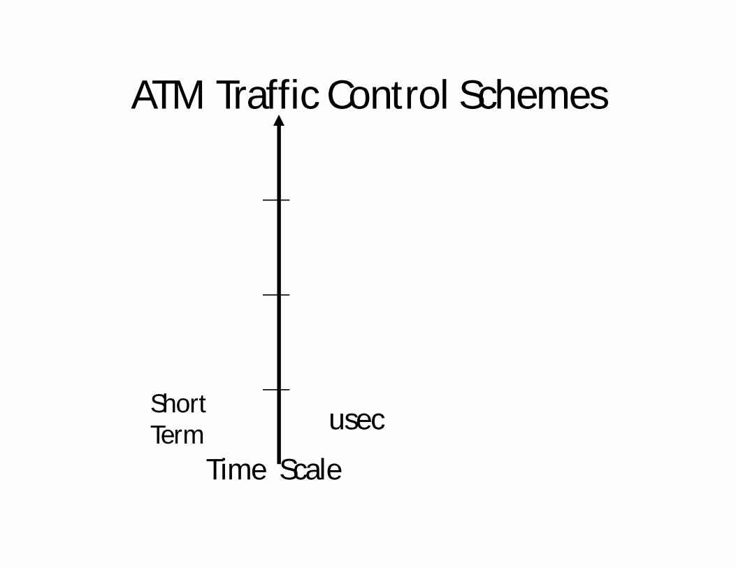
ATM Traffic Control Schemes
Time Scale
ShortTerm usec
ATM Traffic Control Schemes
Time Scale
ShortTerm usec
LongTerm Months, years

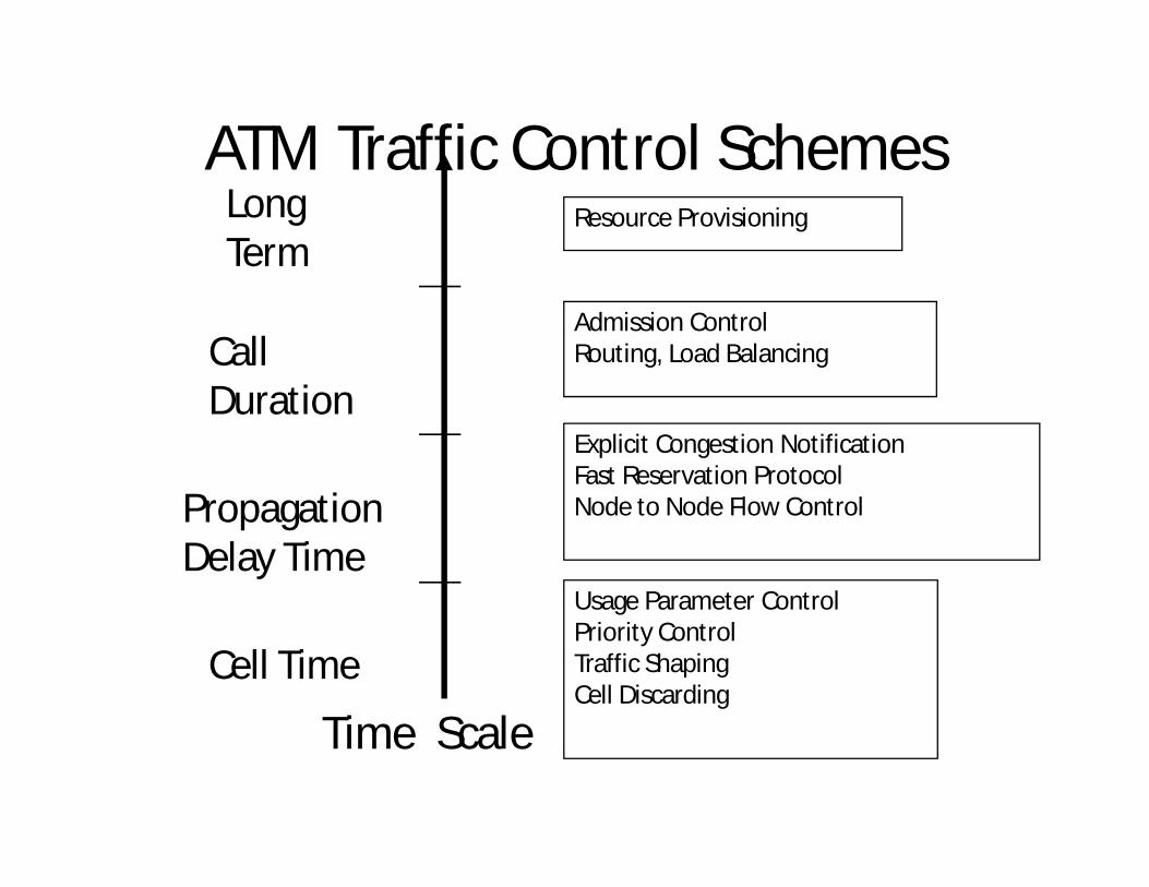
ATM Traffic Control Schemes
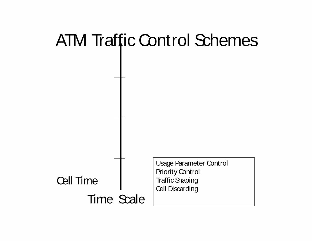
Time ScaleCell Time
Usage Parameter ControlPriority ControlTraffic ShapingCell Discarding
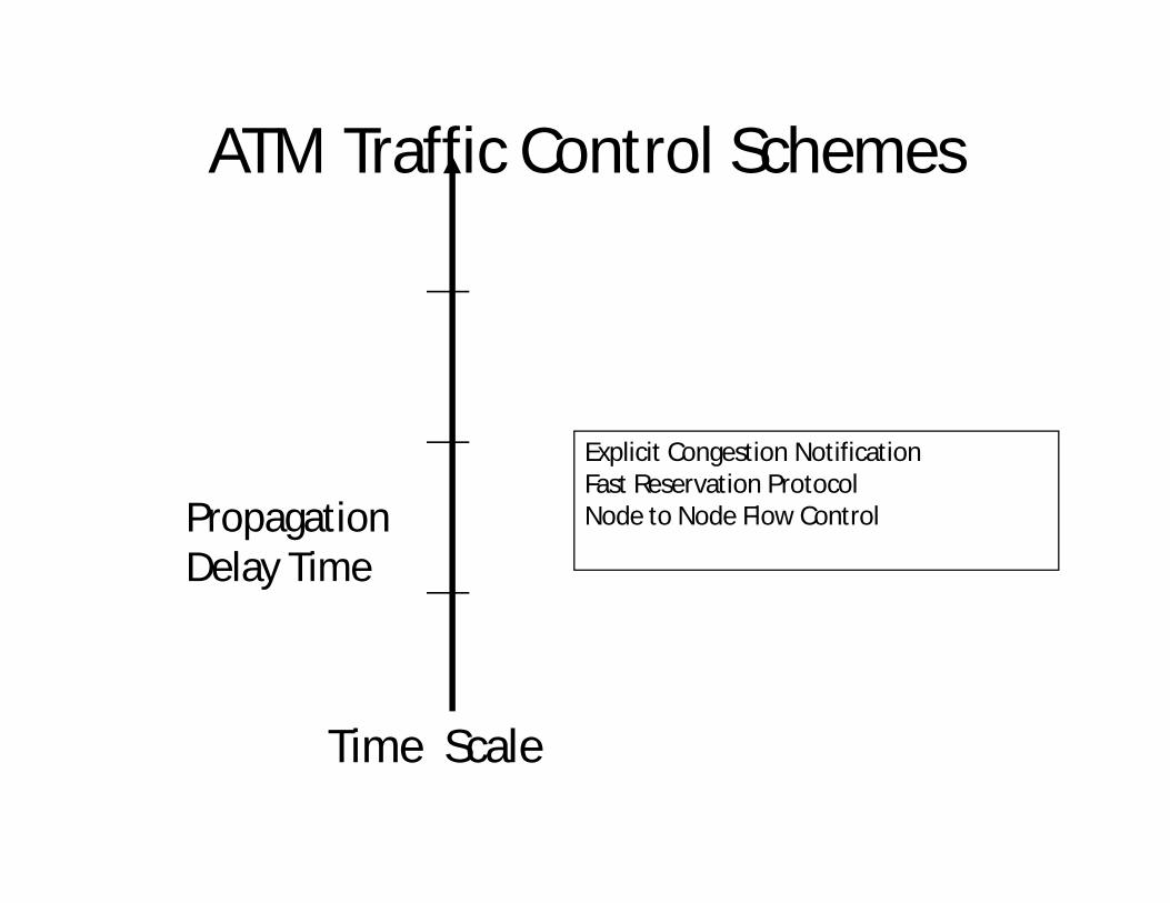
PropagationDelay Time
Explicit Congestion NotificationFast Reservation ProtocolNode to Node Flow Control
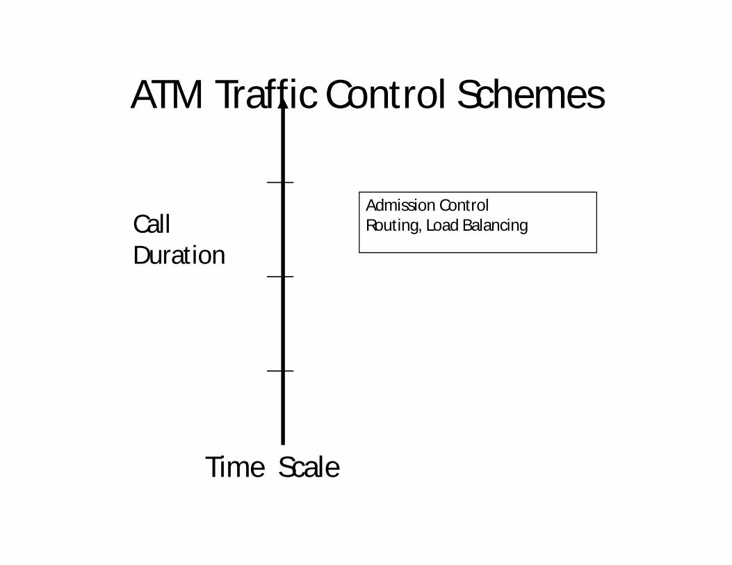
CallDuration
Admission ControlRouting, Load Balancing
LongTerm
Resource Provisioning
ATM Traffic Control Schemes
Time ScaleCell Time
Usage Parameter ControlPriority ControlTraffic ShapingCell Discarding
ATM Traffic Control Schemes
Time Scale
PropagationDelay Time
Explicit Congestion NotificationFast Reservation ProtocolNode to Node Flow Control
ATM Traffic Control Schemes
Time Scale
CallDuration
Admission ControlRouting, Load Balancing
ATM Traffic Control Schemes
Time Scale
LongTerm
Resource Provisioning
ATM Traffic Control Schemes
Time ScaleCell Time
Usage Parameter ControlPriority ControlTraffic ShapingCell Discarding
PropagationDelay Time
Explicit Congestion NotificationFast Reservation ProtocolNode to Node Flow Control
CallDuration
Admission ControlRouting, Load Balancing
LongTerm
Resource Provisioning
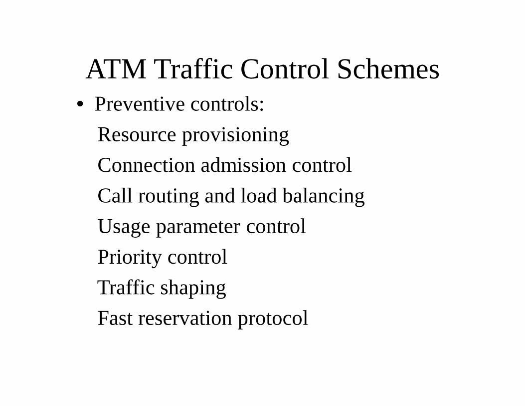
ATM Traffic Control Schemes• Preventive controls:
Resource provisioningConnection admission controlCall routing and load balancingUsage parameter controlPriority controlTraffic shapingFast reservation protocol
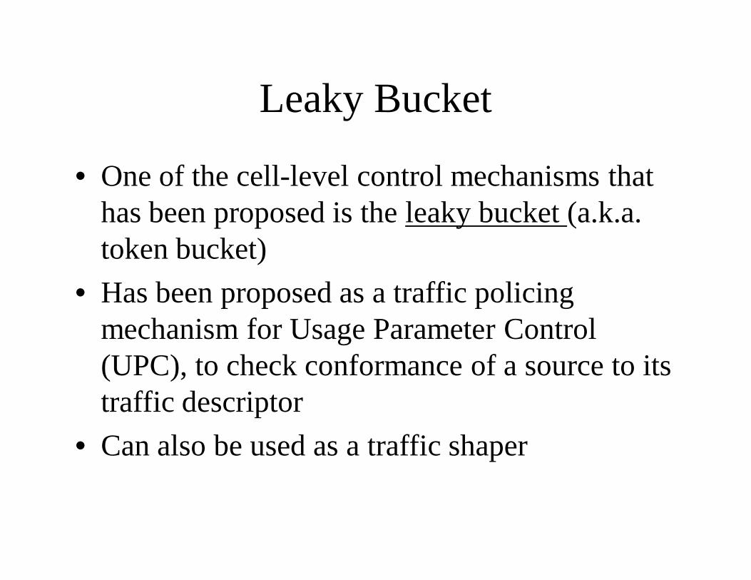
Leaky Bucket
• One of the cell-level control mechanisms that has been proposed is the leaky bucket (a.k.a. token bucket)
• Has been proposed as a traffic policing mechanism for Usage Parameter Control (UPC), to check conformance of a source to its traffic descriptor
• Can also be used as a traffic shaper
Leaky Bucket (Cont’d)
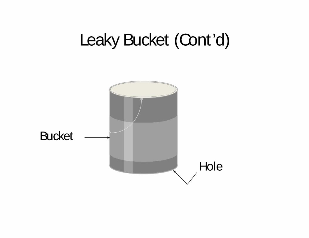
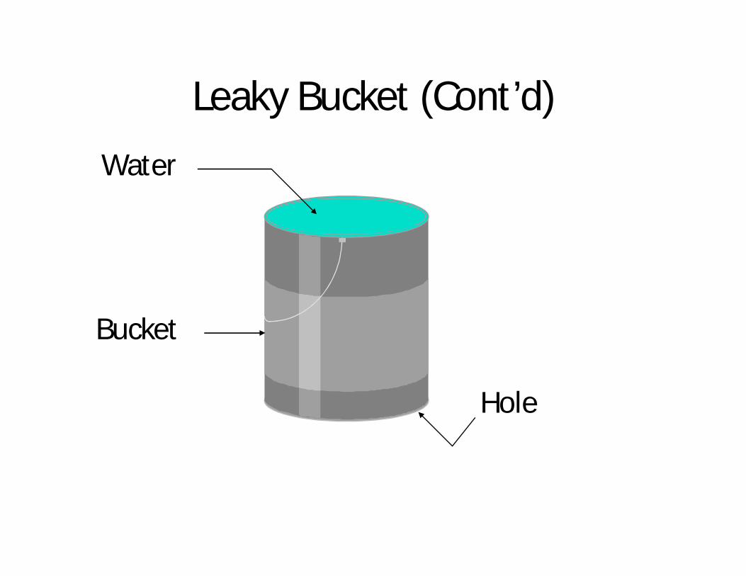
• Think of a bucket (pail) with a small hole in the bottom
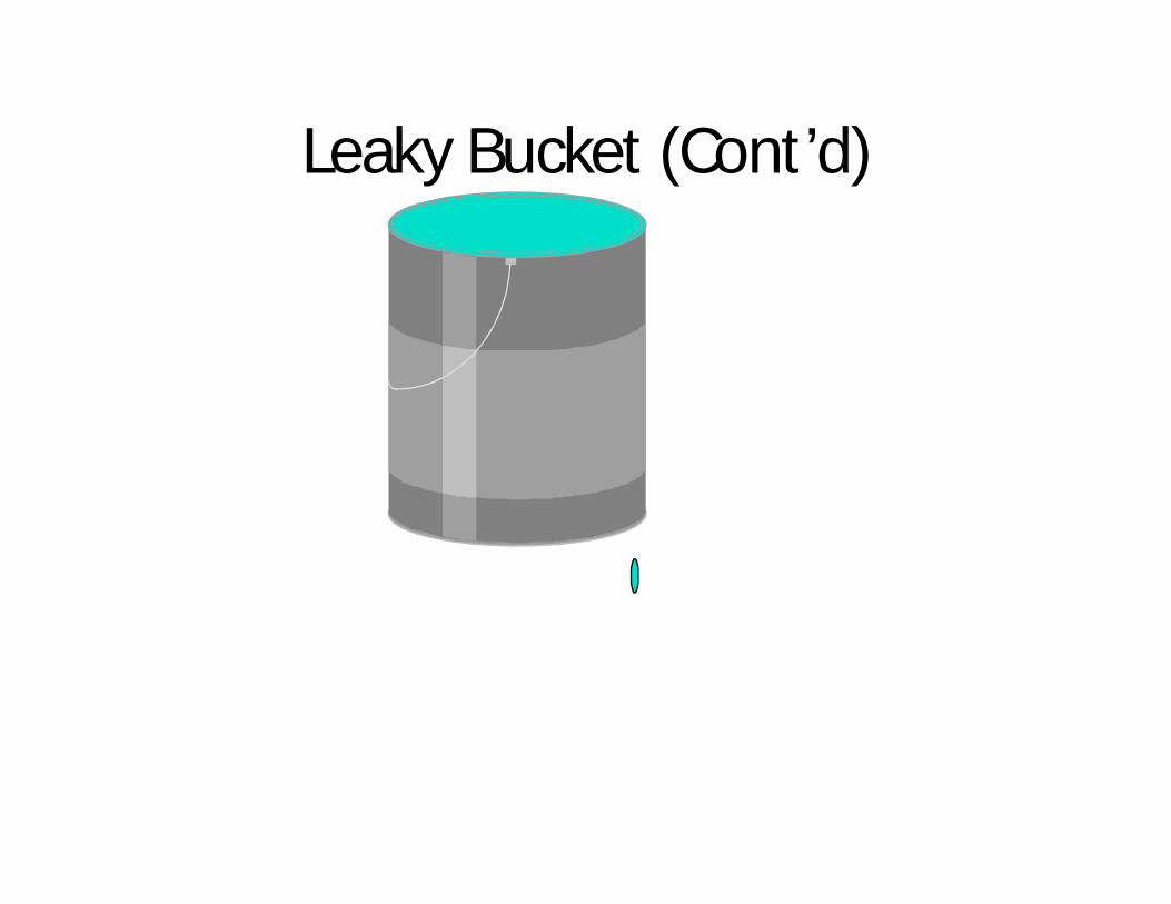
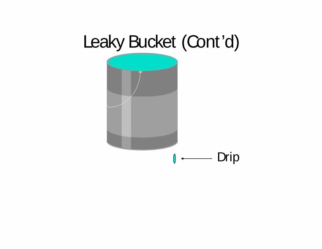
• You fill the bucket with water• Water drips out the bottom at a nice constant
rate: drip, drip, drip...
Leaky Bucket (Cont’d)
Leaky Bucket (Cont’d)
Bucket
Leaky Bucket (Cont’d)
Bucket
Empty
Leaky Bucket (Cont’d)
Bucket
Hole
Leaky Bucket (Cont’d)
Bucket
Water
Hole
Leaky Bucket (Cont’d)
Leaky Bucket (Cont’d)
Drip

Leaky Bucket (Cont’d)
Leaky Bucket (Cont’d)
Leaky Bucket (Cont’d)
Leaky Bucket (Cont’d)
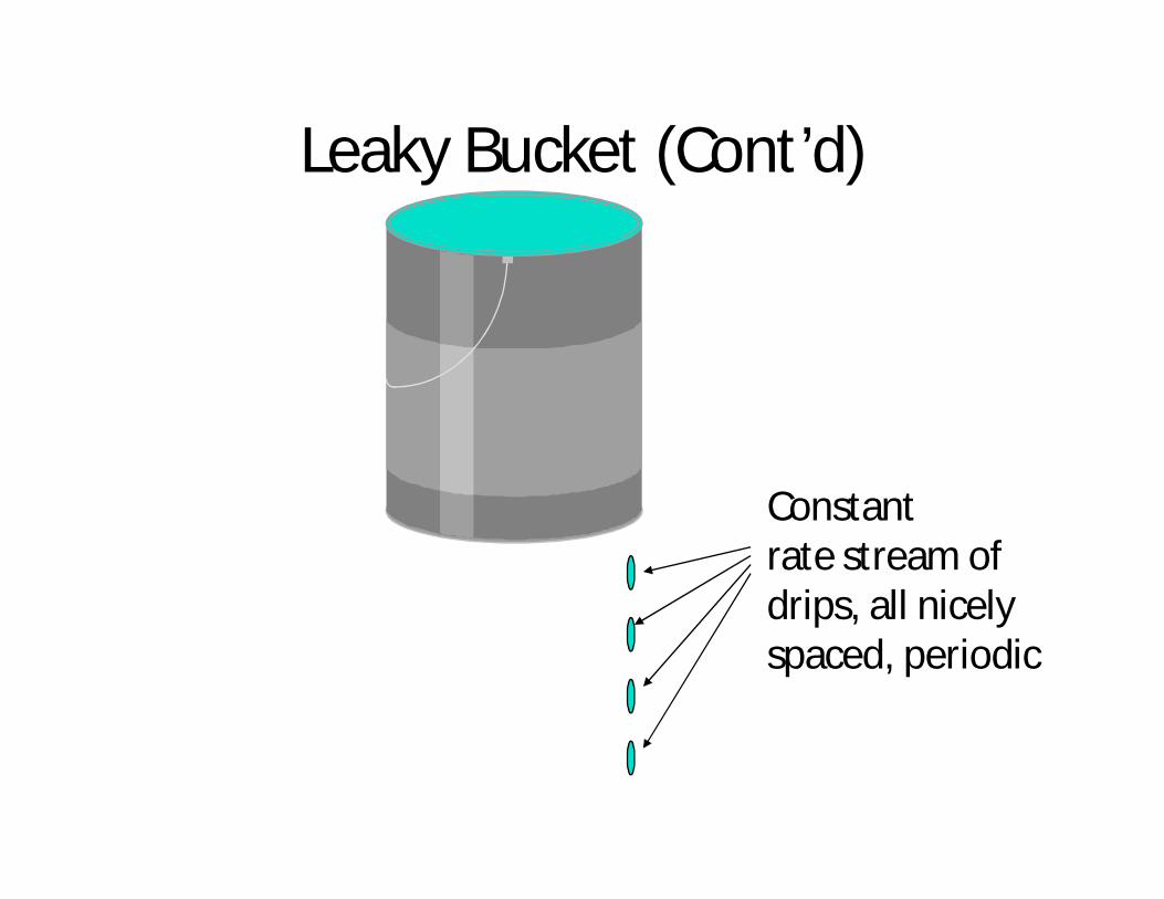
Constantrate stream ofdrips, all nicelyspaced, periodic
Leaky Bucket (Cont’d)
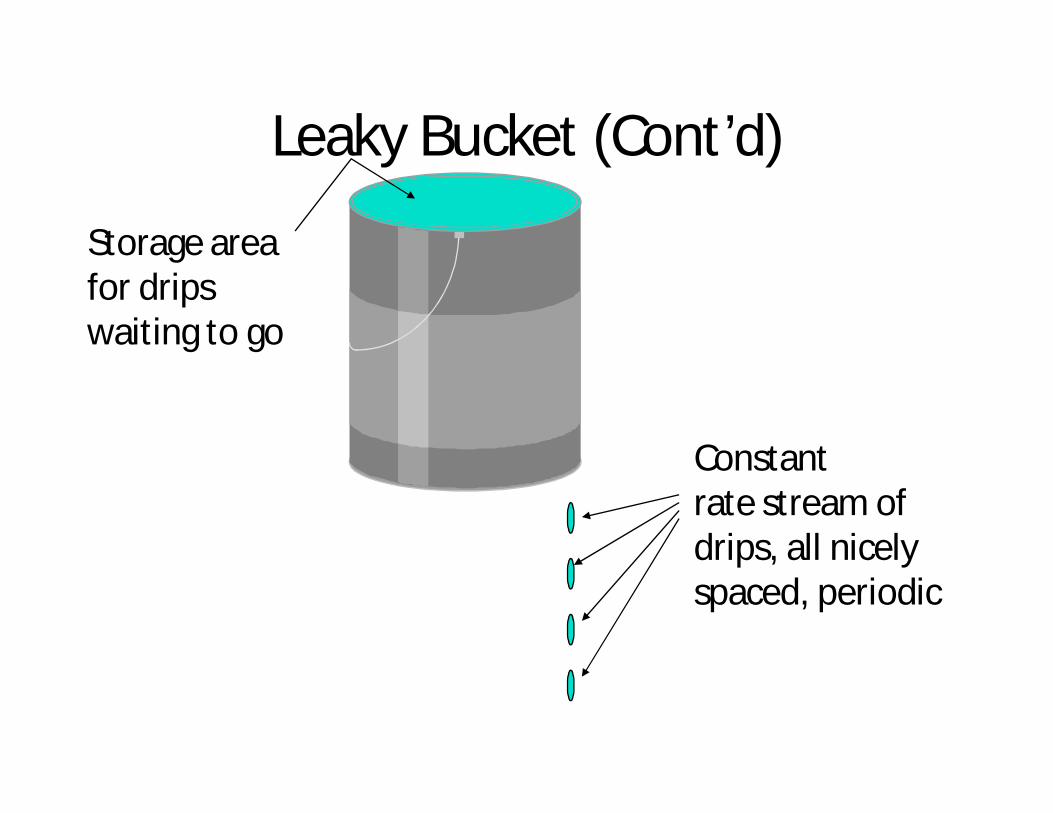
Constantrate stream ofdrips, all nicelyspaced, periodic
Storage areafor dripswaiting to go
Leaky Bucket (Cont’d)
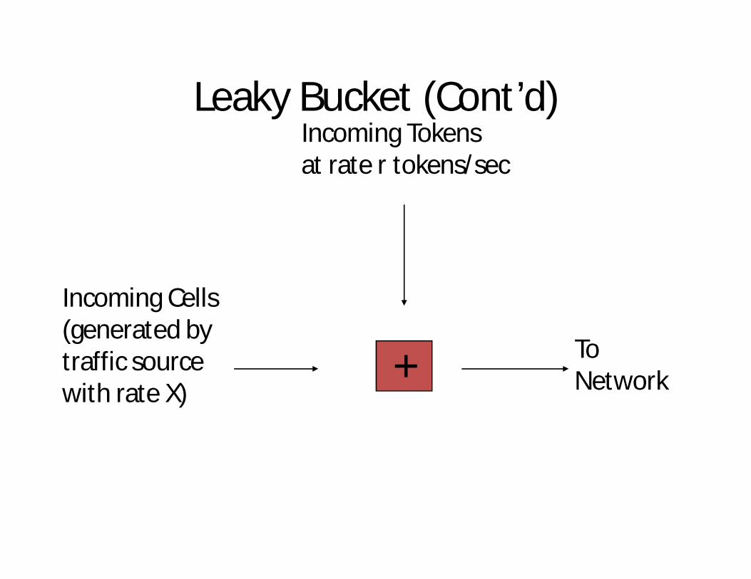
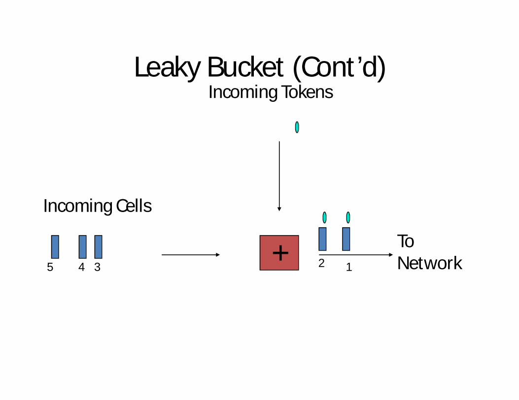
Incoming Cells(generated bytraffic sourcewith rate X)
Incoming Tokensat rate r tokens/sec
+ ToNetwork
Leaky Bucket (Cont’d)
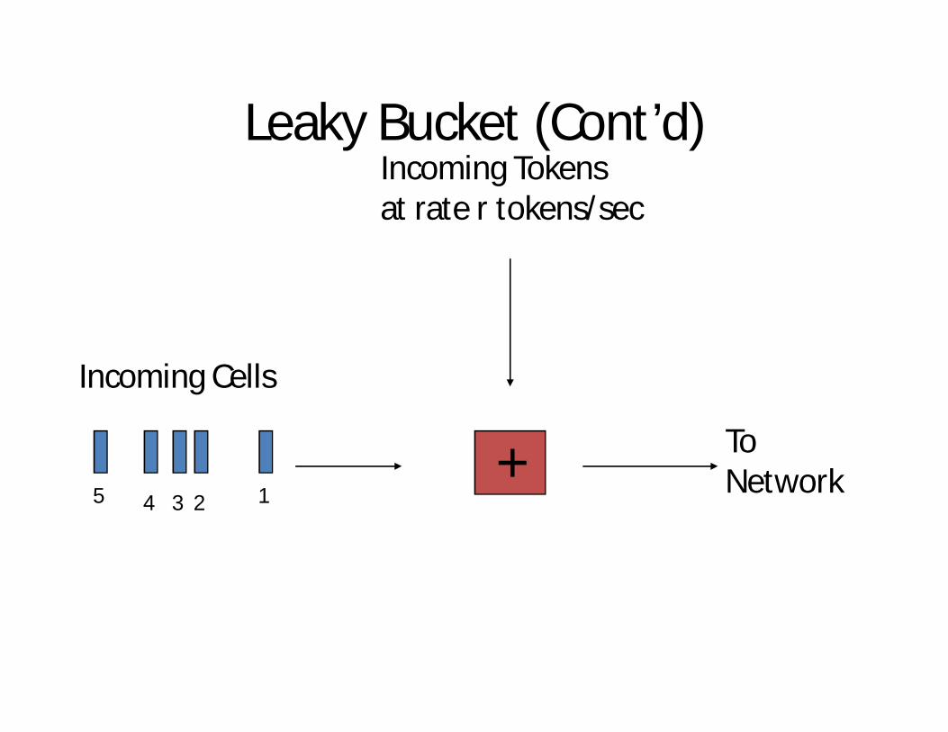
Incoming Cells
Incoming Tokensat rate r tokens/sec
+ ToNetwork12345
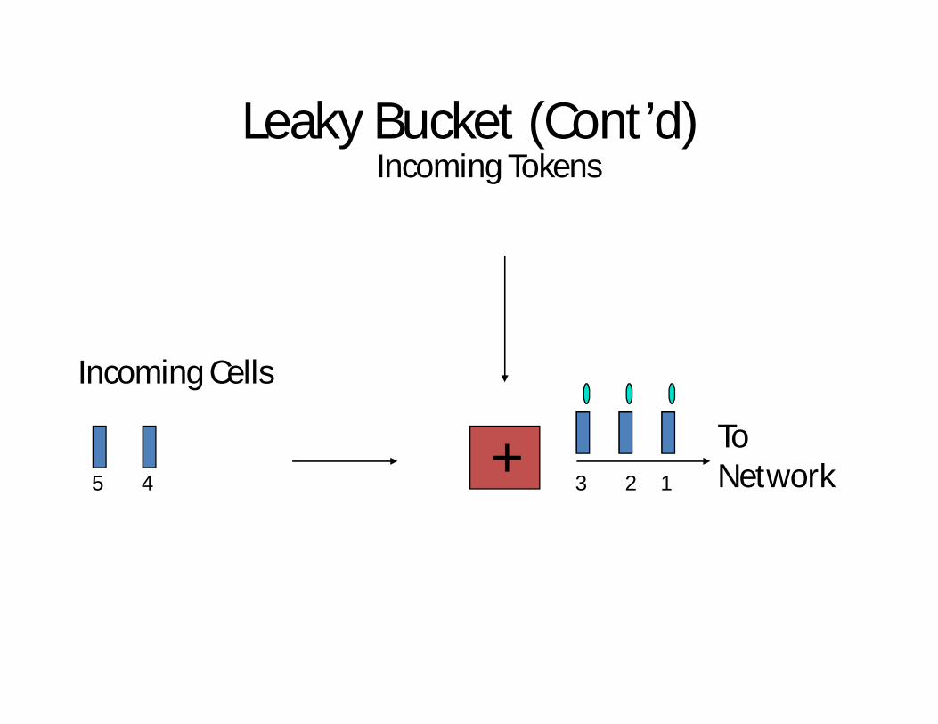
Leaky Bucket (Cont’d)
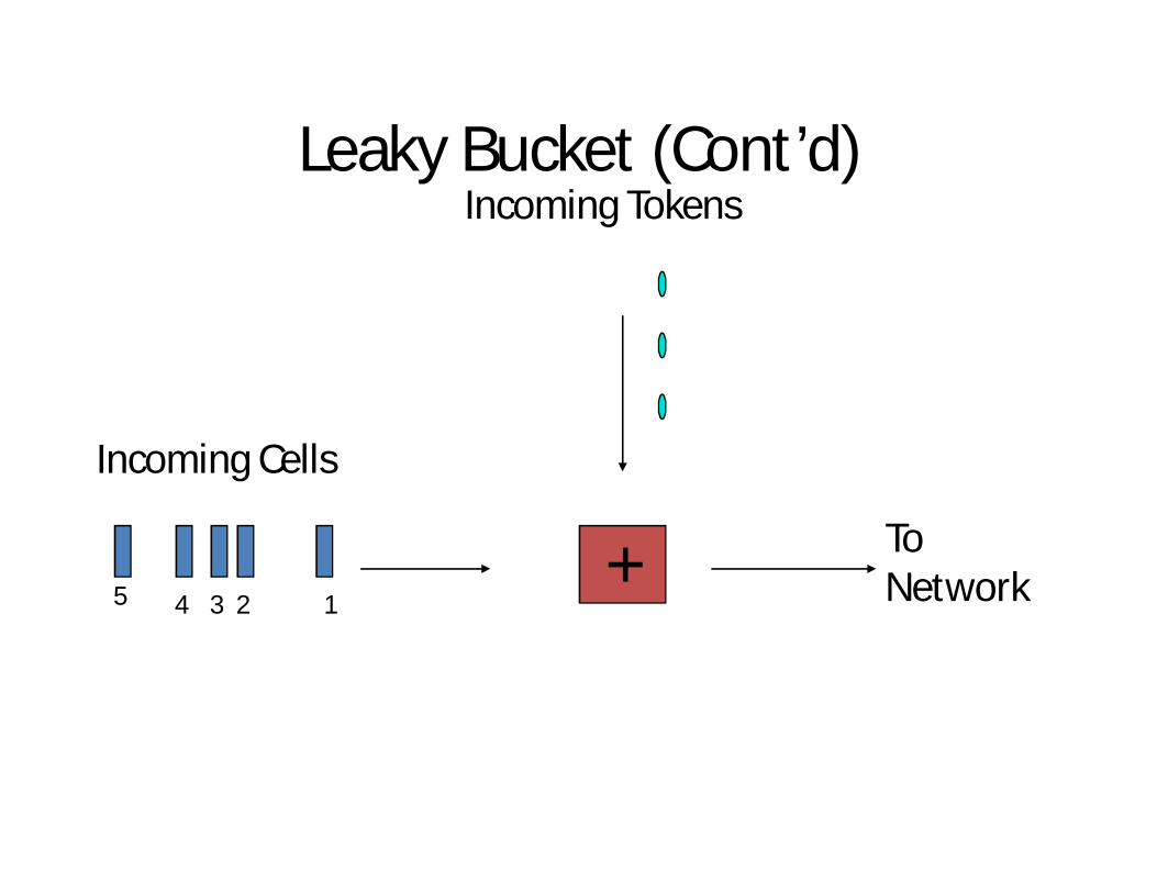
Incoming Cells
Incoming Tokens
+ ToNetwork12345
Leaky Bucket (Cont’d)
Incoming Cells
Incoming Tokens
+ ToNetwork12345
Leaky Bucket (Cont’d)
Incoming Cells
Incoming Tokens
+ ToNetwork12345
Leaky Bucket (Cont’d)
Incoming Cells
Incoming Tokens
+ ToNetwork12345
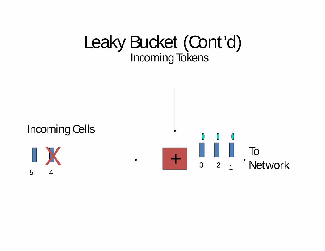
Leaky Bucket (Cont’d)
Incoming Cells
Incoming Tokens
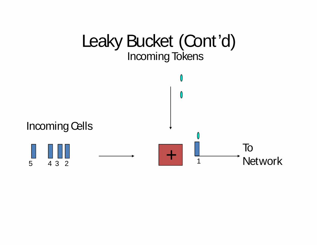
+ ToNetworkX 123
45

Leaky Bucket (Cont’d)
Incoming Cells
Incoming Tokens
+ ToNetworkXX 123
45
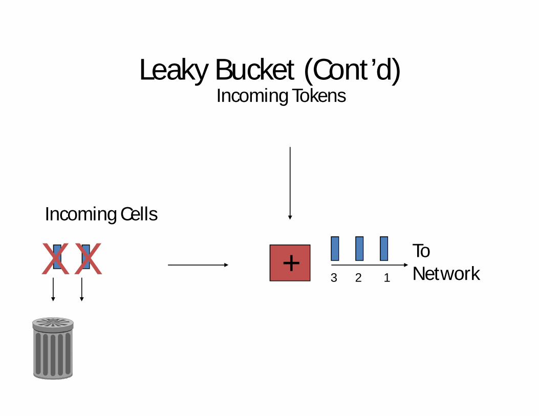
Leaky Bucket (Cont’d)
Incoming Cells
Incoming Tokens
+ ToNetworkXX 123
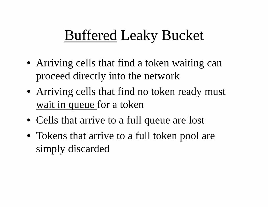
Buffered Leaky Bucket
• Arriving cells that find a token waiting can proceed directly into the network
• Arriving cells that find no token ready must wait in queue for a token
• Cells that arrive to a full queue are lost• Tokens that arrive to a full token pool are
simply discarded
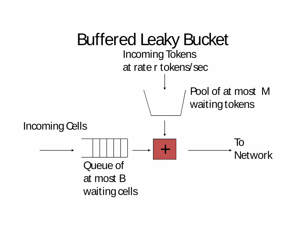
Buffered Leaky Bucket
Incoming Cells
Incoming Tokensat rate r tokens/sec
+ ToNetwork
Queue ofat most Bwaiting cells
Pool of at most Mwaiting tokens
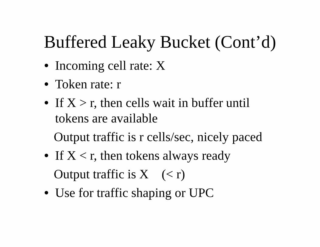
Buffered Leaky Bucket (Cont’d)• Incoming cell rate: X• Token rate: r• If X > r, then cells wait in buffer until
tokens are availableOutput traffic is r cells/sec, nicely paced
• If X < r, then tokens always readyOutput traffic is X (< r)
• Use for traffic shaping or UPC
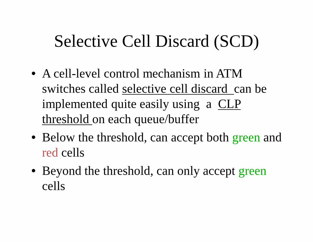
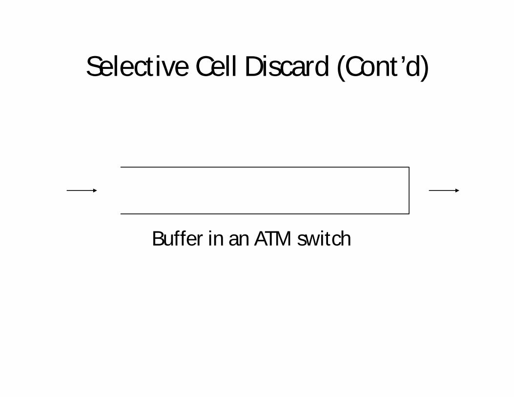
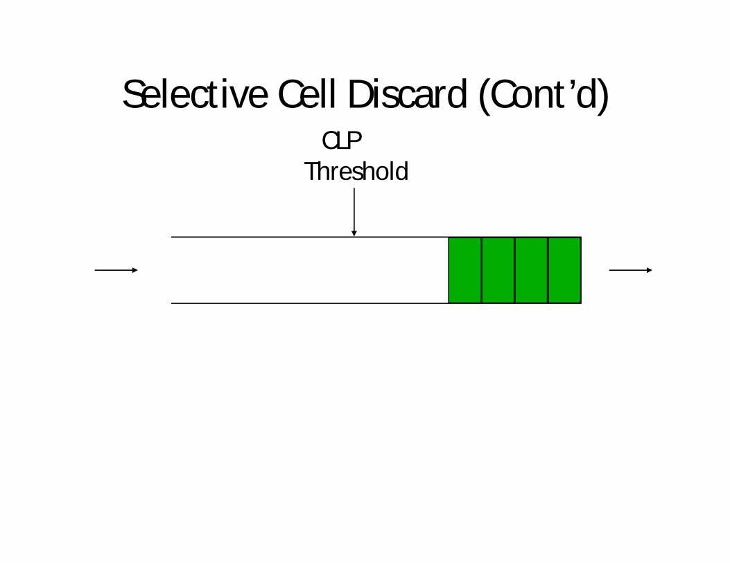
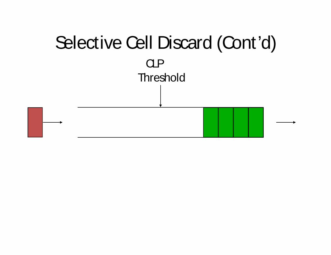
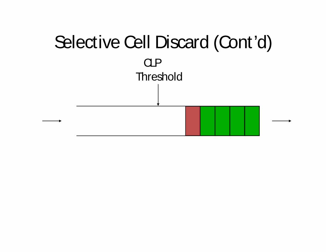
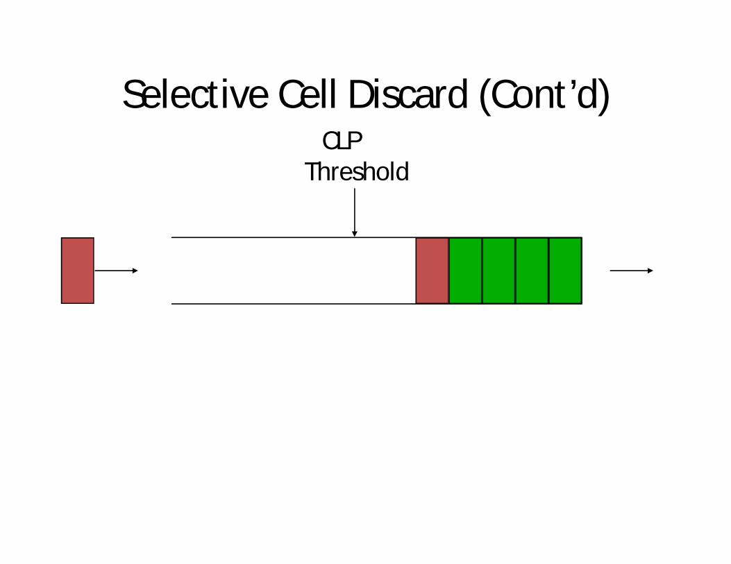
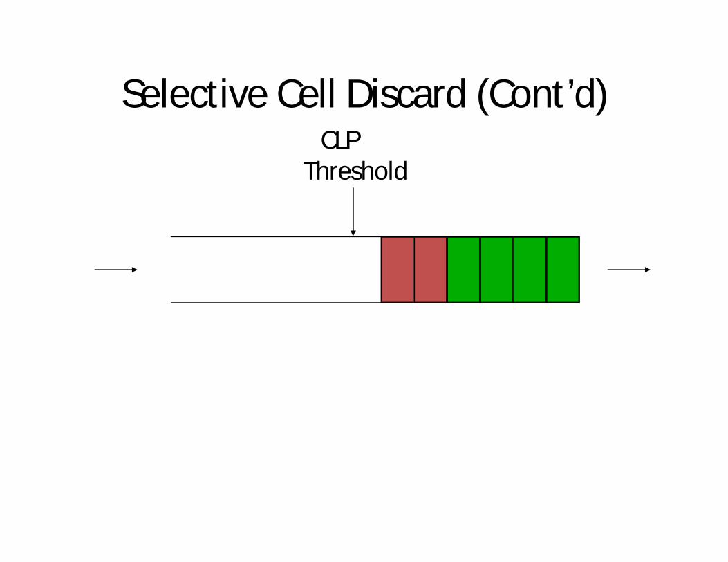
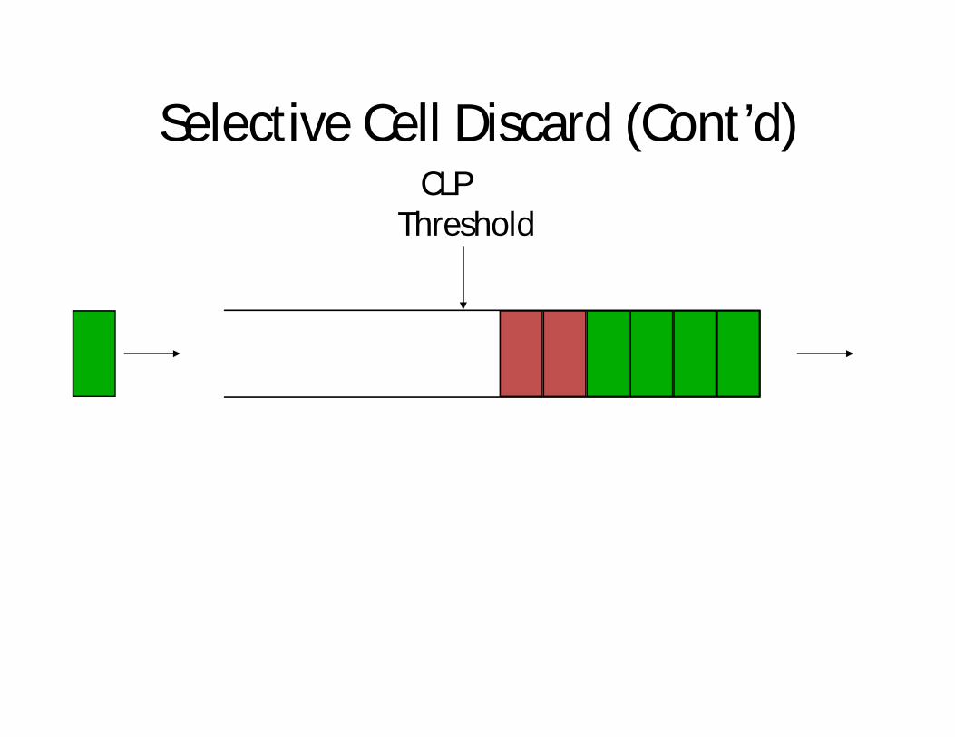
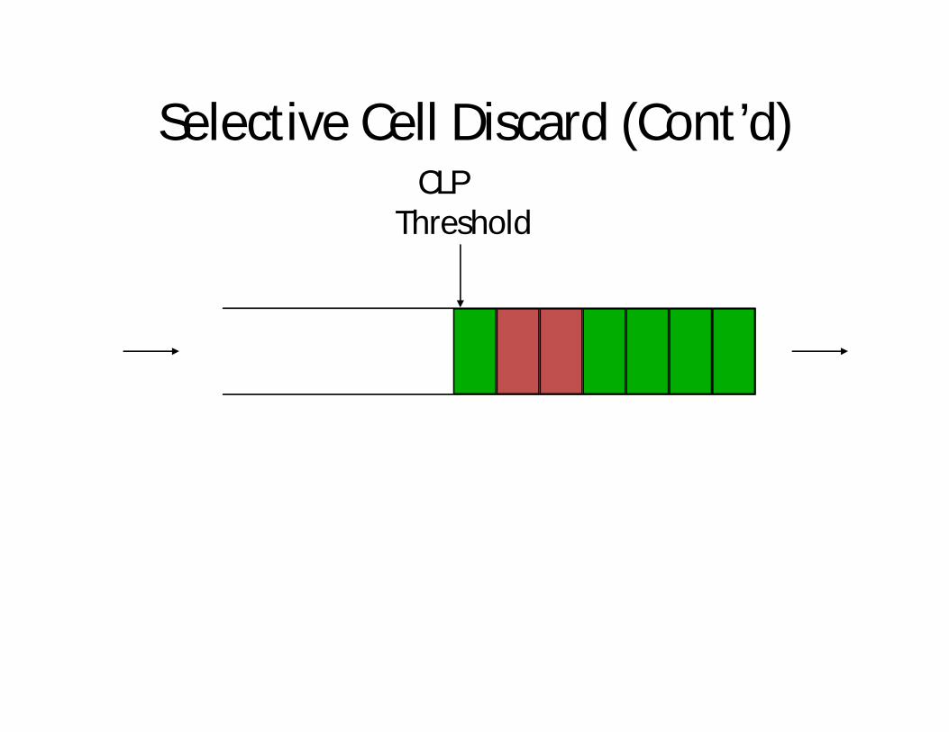
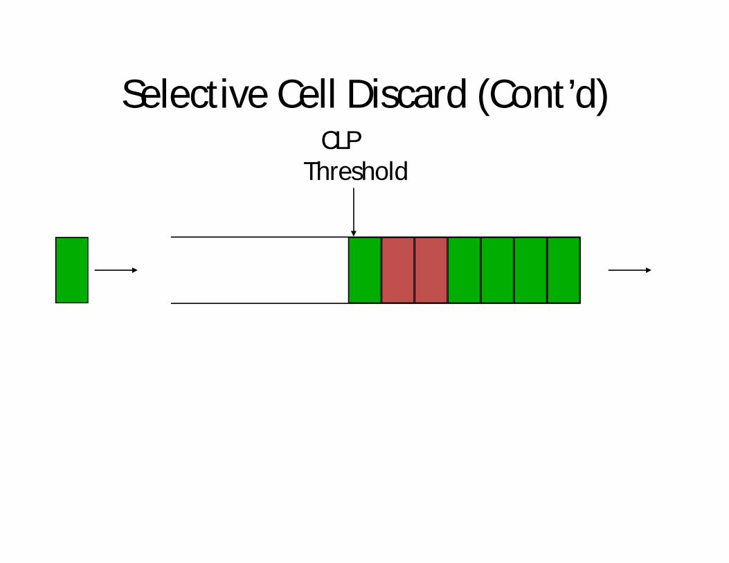
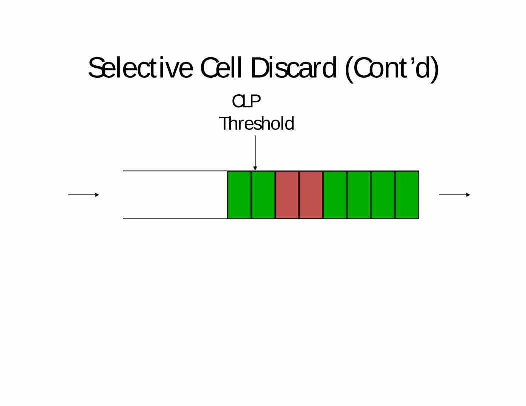
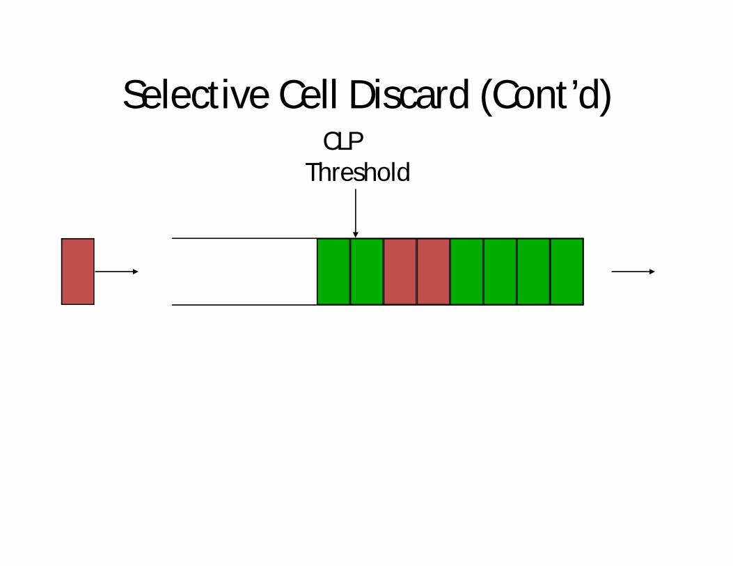
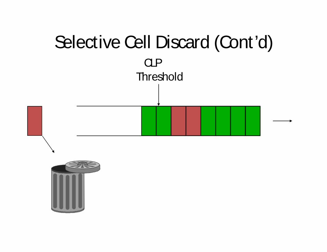
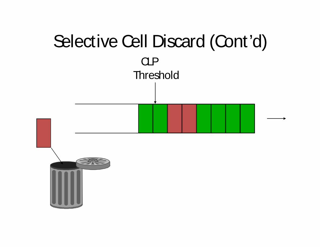
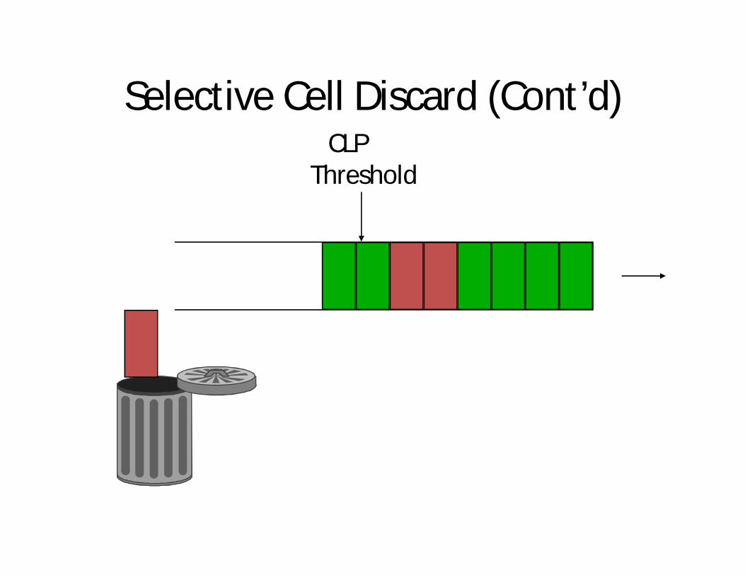
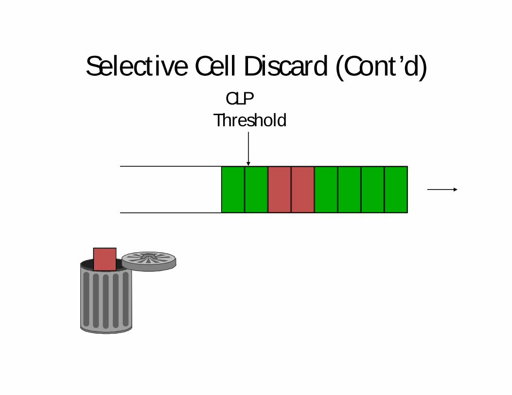
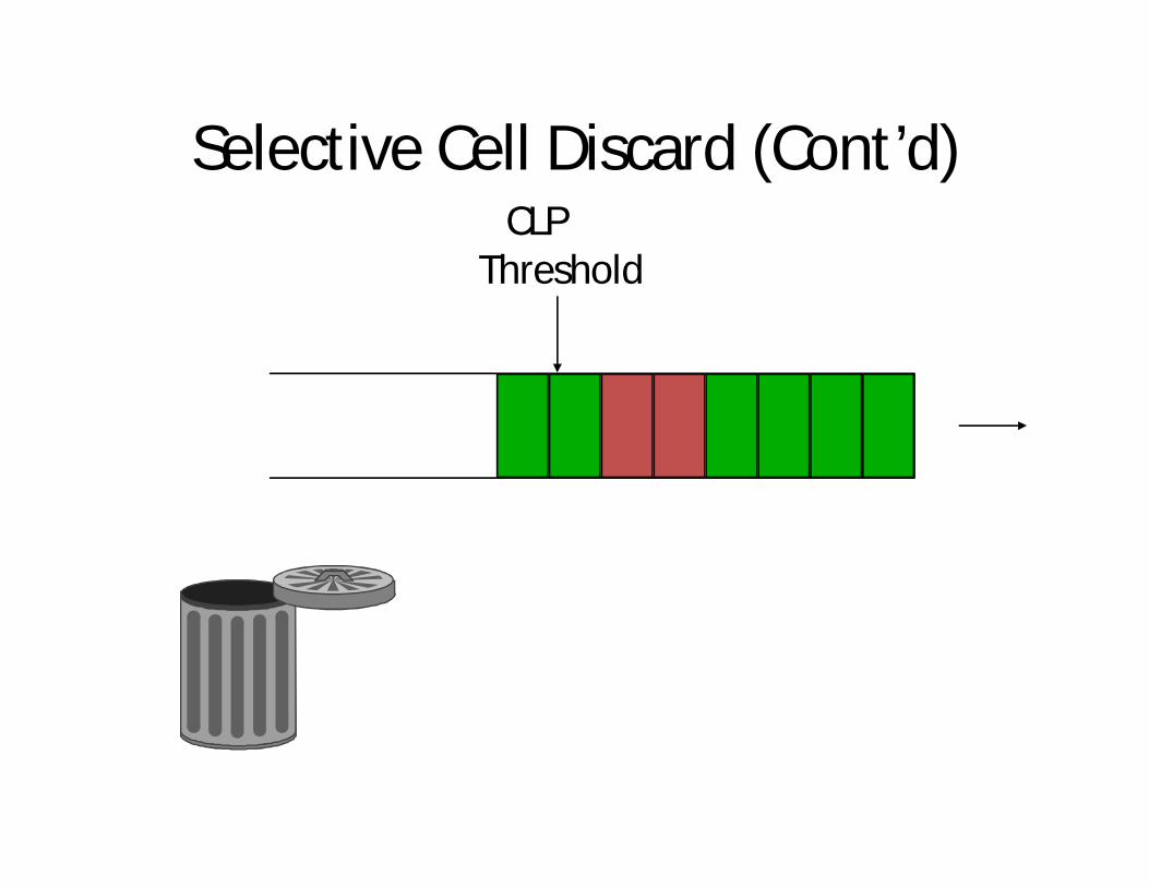
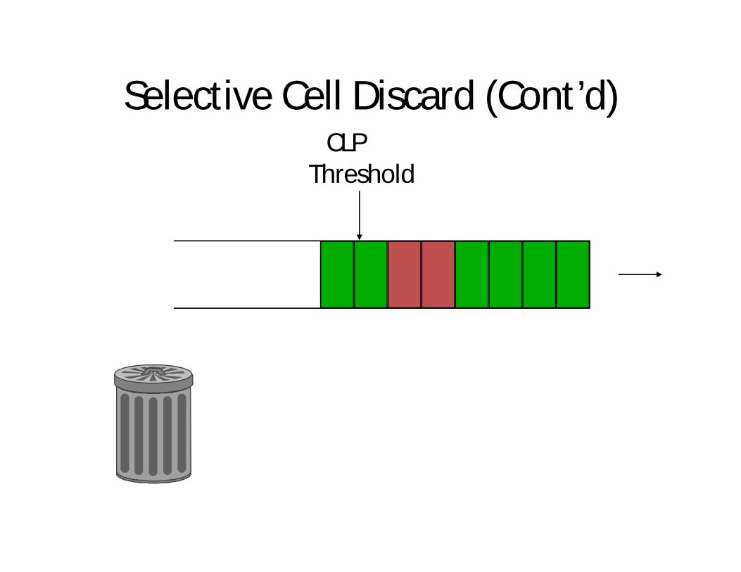
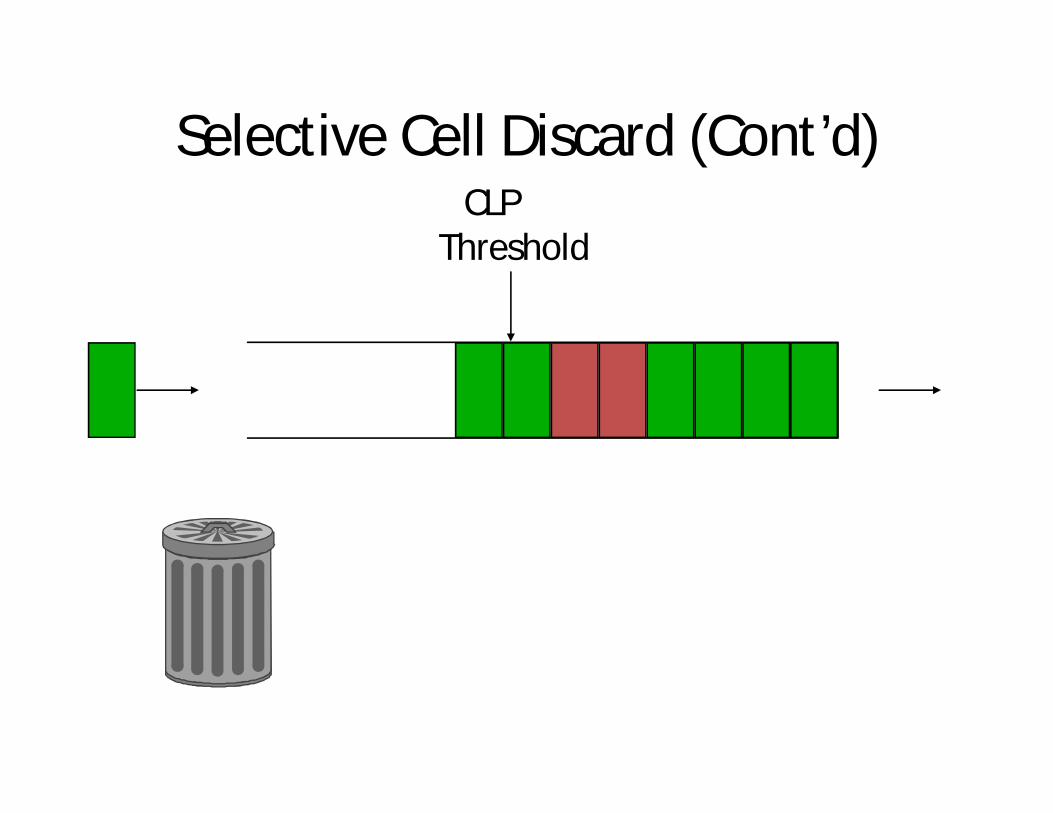
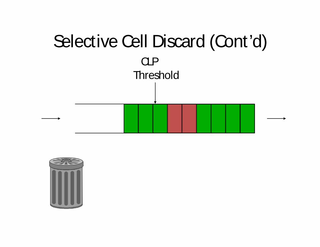
Selective Cell Discard (SCD)
• A cell-level control mechanism in ATM switches called selective cell discard can be implemented quite easily using a CLP threshold on each queue/buffer
• Below the threshold, can accept both green and red cells
• Beyond the threshold, can only accept greencells

Selective Cell Discard (Cont’d)
Buffer in an ATM switch
Selective Cell Discard (Cont’d)
Buffer in an ATM switch
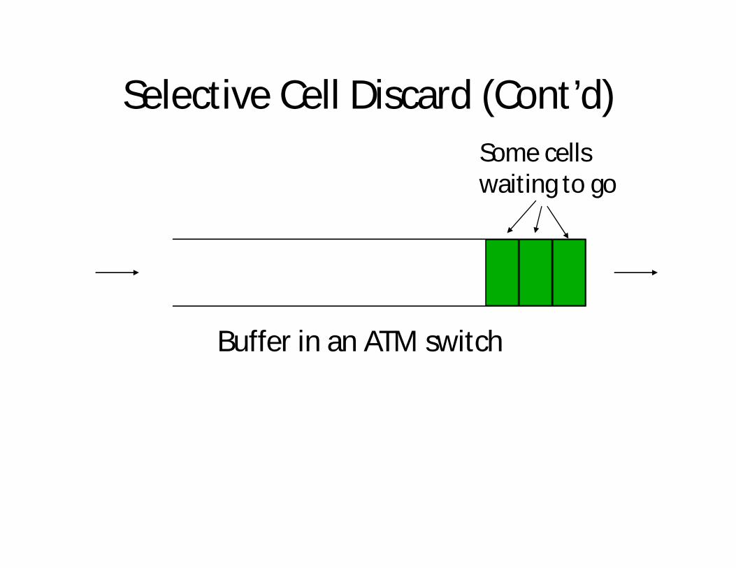
Selective Cell Discard (Cont’d)
Buffer in an ATM switch
Some cellswaiting to go
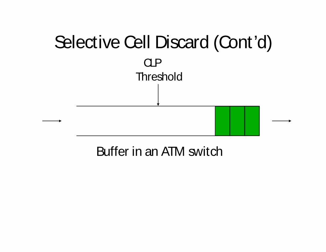
Selective Cell Discard (Cont’d)CLP
Threshold
Buffer in an ATM switch
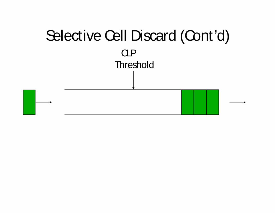
Selective Cell Discard (Cont’d)CLP
Threshold
Selective Cell Discard (Cont’d)CLP
Threshold
Selective Cell Discard (Cont’d)CLP
Threshold
Selective Cell Discard (Cont’d)CLP
Threshold
Selective Cell Discard (Cont’d)CLP
Threshold
Selective Cell Discard (Cont’d)CLP
Threshold
Selective Cell Discard (Cont’d)CLP
Threshold
Selective Cell Discard (Cont’d)CLP
Threshold
Selective Cell Discard (Cont’d)CLP
Threshold
Selective Cell Discard (Cont’d)CLP
Threshold
Selective Cell Discard (Cont’d)CLP
Threshold

Selective Cell Discard (Cont’d)CLP
Threshold
Selective Cell Discard (Cont’d)CLP
Threshold
Selective Cell Discard (Cont’d)CLP
Threshold
Selective Cell Discard (Cont’d)CLP
Threshold
Selective Cell Discard (Cont’d)CLP
Threshold
Selective Cell Discard (Cont’d)CLP
Threshold
Selective Cell Discard (Cont’d)CLP
Threshold
Selective Cell Discard (Cont’d)CLP
Threshold
Selective Cell Discard (Cont’d)CLP
Threshold
Explicit Congestion Notification
• There are some proposals to use reactive congestion control approaches for end-to-end flow control in ATM
• One of the mechanisms proposed is called Explicit Forward Congestion Notification (EFCN) (or EFCI, for Explicit Forward Congestion Indication)
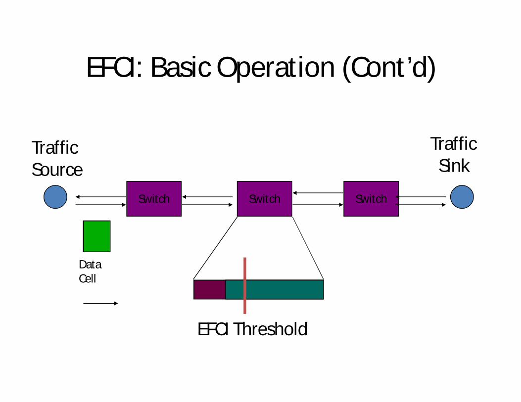
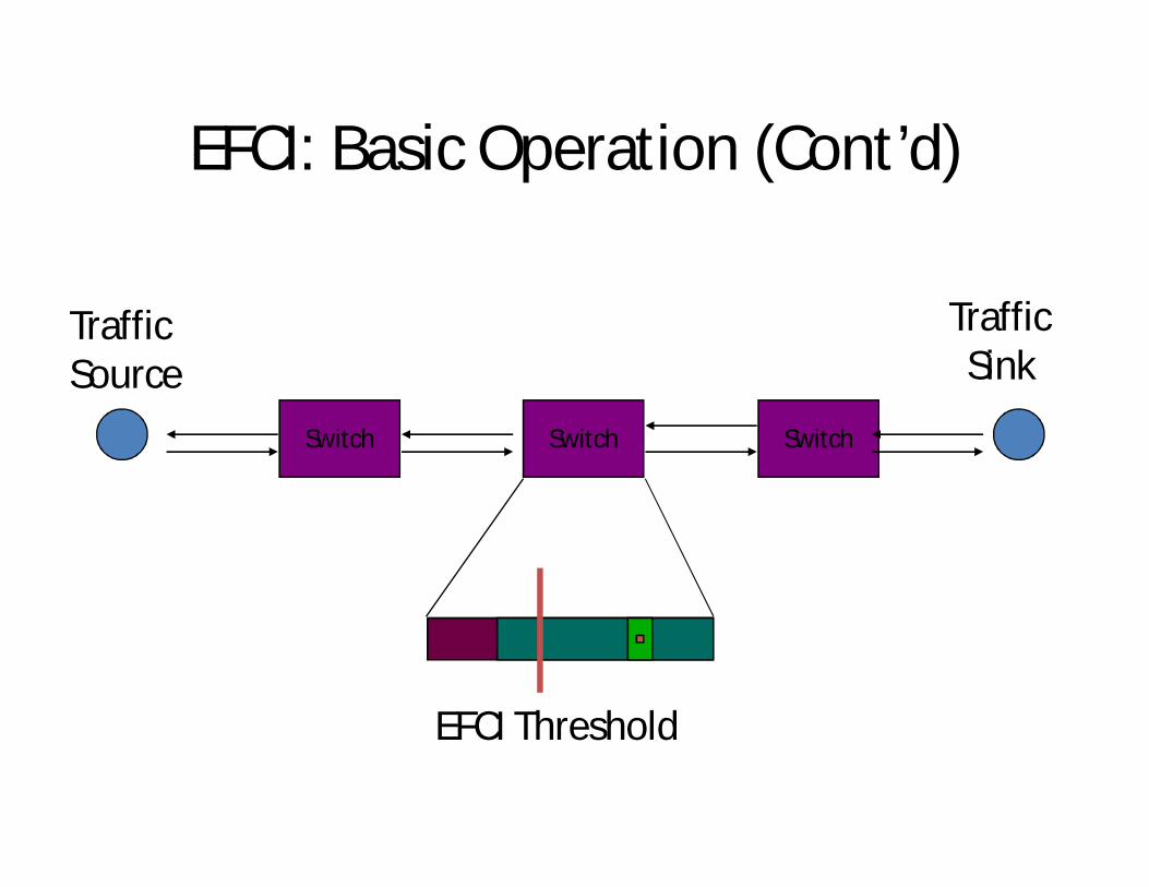
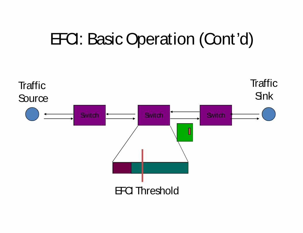
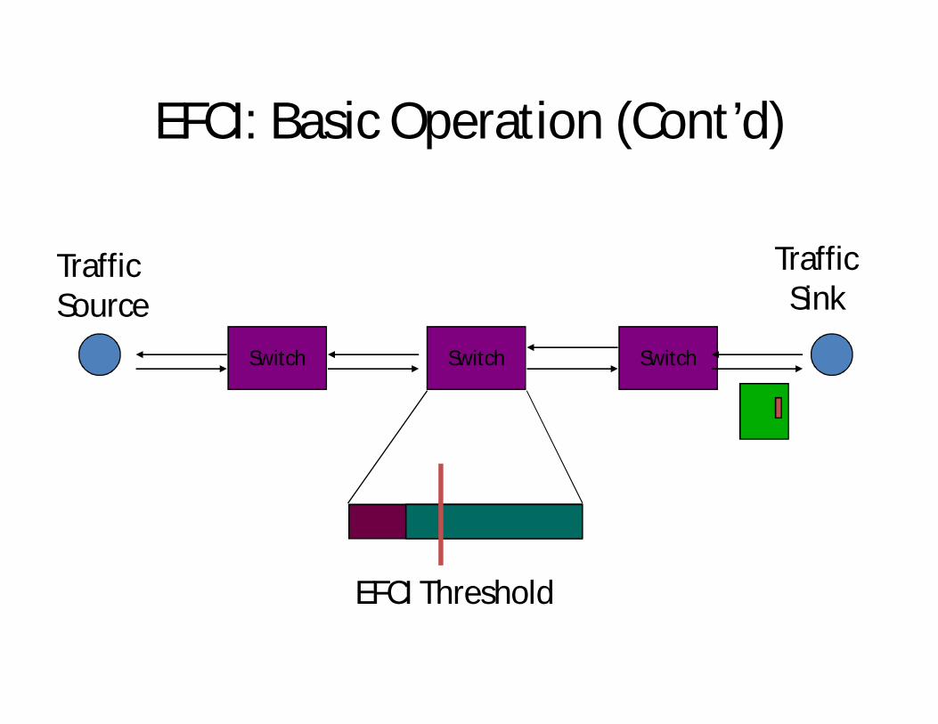
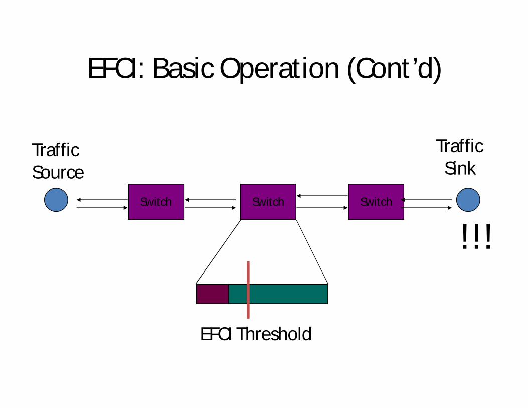
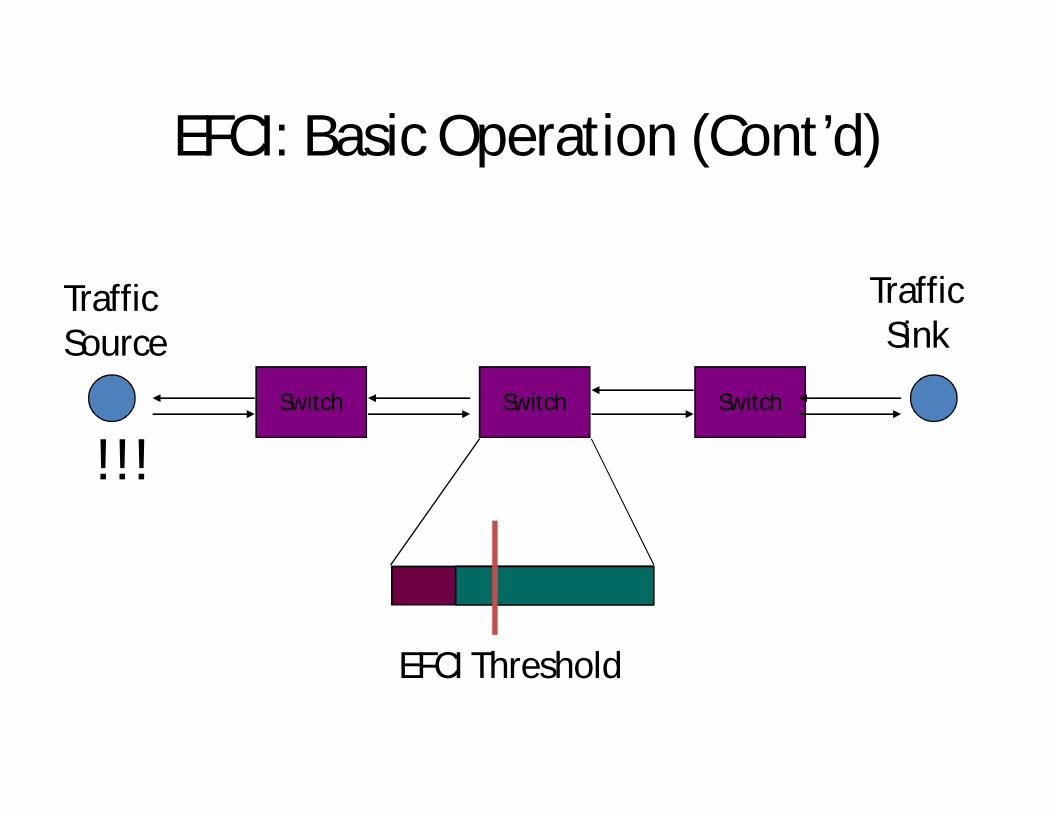
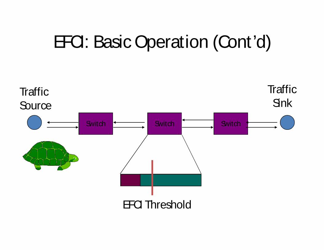
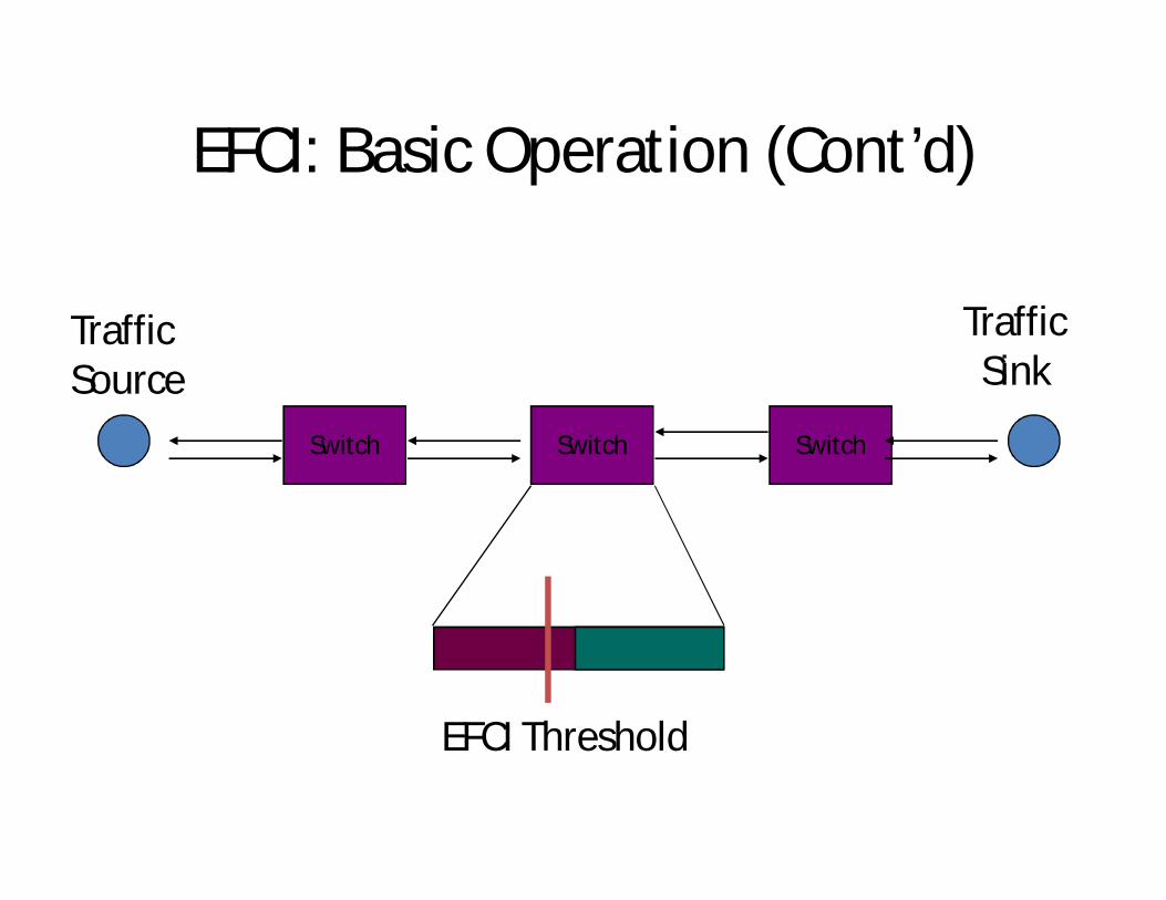
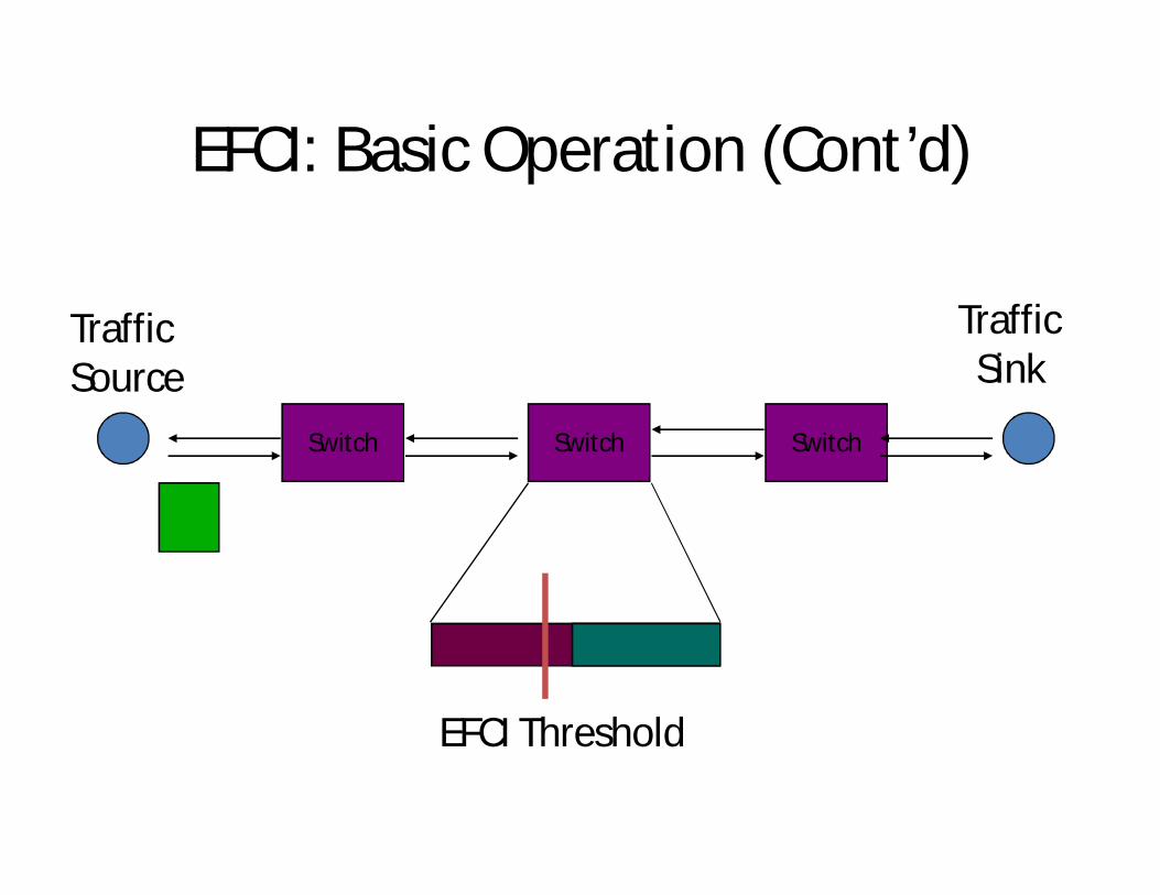
EFCI: Basic Operation
• Switches can detect the onset of congestion (e.g., buffers filling up)
• Switches set a control bit in cell headers to indicate this congestion condition
• Sources react by reducing the volume of traffic that they are sending through that switch
• Suitable for VBR or ABR traffic
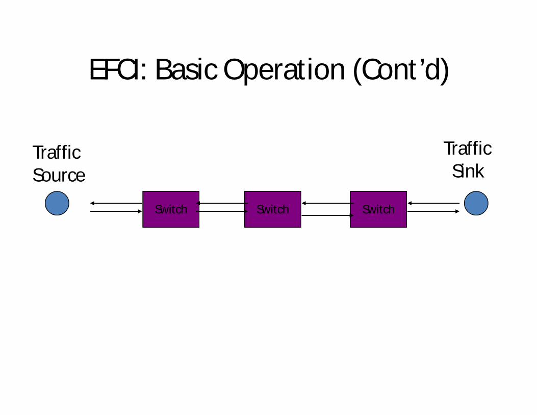
EFCI: Basic Operation (Cont’d)
Traffic Source
Traffic Sink
Switch Switch Switch
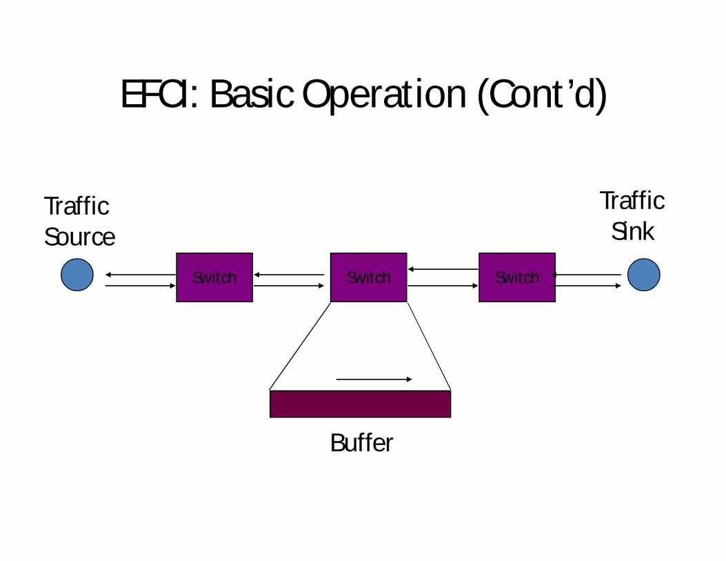
EFCI: Basic Operation (Cont’d)
Traffic Source
Traffic Sink
Switch Switch Switch
Buffer
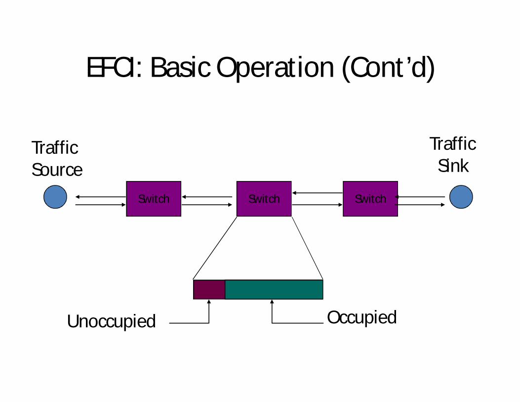
EFCI: Basic Operation (Cont’d)
Traffic Source
Traffic Sink
Switch Switch Switch
OccupiedUnoccupied
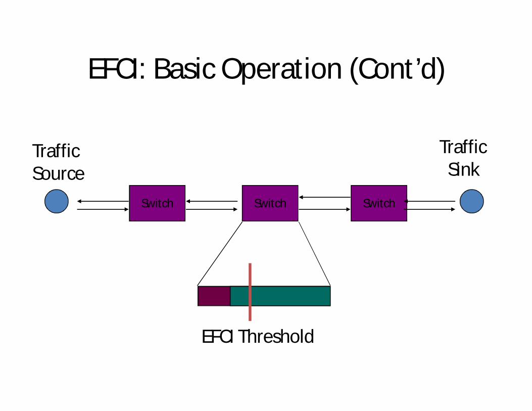
EFCI: Basic Operation (Cont’d)
Traffic Source
Traffic Sink
Switch Switch Switch
EFCI Threshold
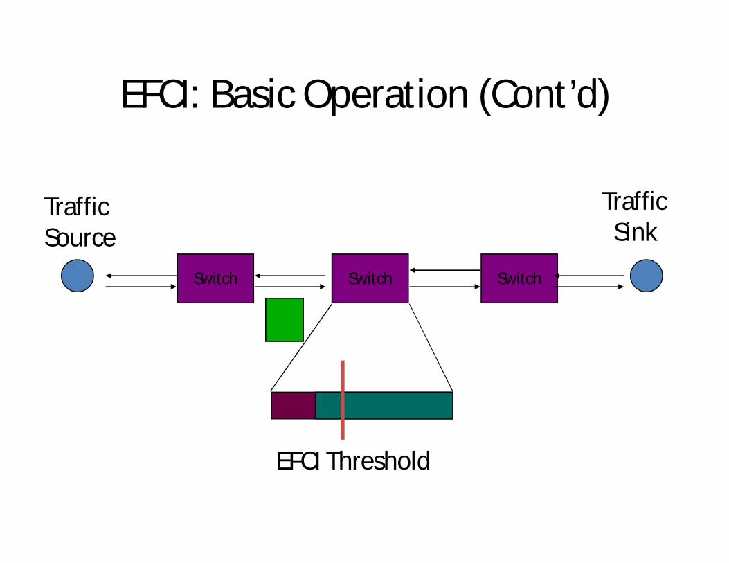
EFCI: Basic Operation (Cont’d)
Traffic Source
Traffic Sink
Switch Switch Switch
EFCI Threshold
DataCell
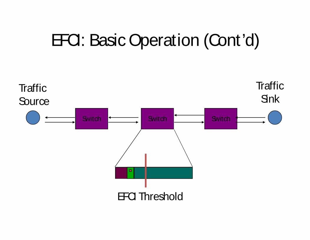
EFCI: Basic Operation (Cont’d)
Traffic Source
Traffic Sink
Switch Switch Switch
EFCI Threshold
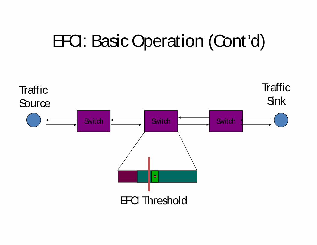
EFCI: Basic Operation (Cont’d)
Traffic Source
Traffic Sink
Switch Switch Switch
EFCI Threshold
EFCI: Basic Operation (Cont’d)
Traffic Source
Traffic Sink
Switch Switch Switch
EFCI Threshold
EFCI: Basic Operation (Cont’d)
Traffic Source
Traffic Sink
Switch Switch Switch
EFCI Threshold

EFCI: Basic Operation (Cont’d)
Traffic Source
Traffic Sink
Switch Switch Switch
EFCI Threshold
EFCI: Basic Operation (Cont’d)
Traffic Source
Traffic Sink
Switch Switch Switch
EFCI Threshold
EFCI: Basic Operation (Cont’d)
Traffic Source
Traffic Sink
Switch Switch Switch
EFCI Threshold
EFCI: Basic Operation (Cont’d)
Traffic Source
Traffic Sink
Switch Switch Switch
EFCI Threshold
!!!
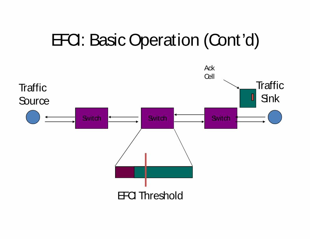
EFCI: Basic Operation (Cont’d)
Traffic Source
Traffic Sink
Switch Switch Switch
EFCI Threshold
AckCell
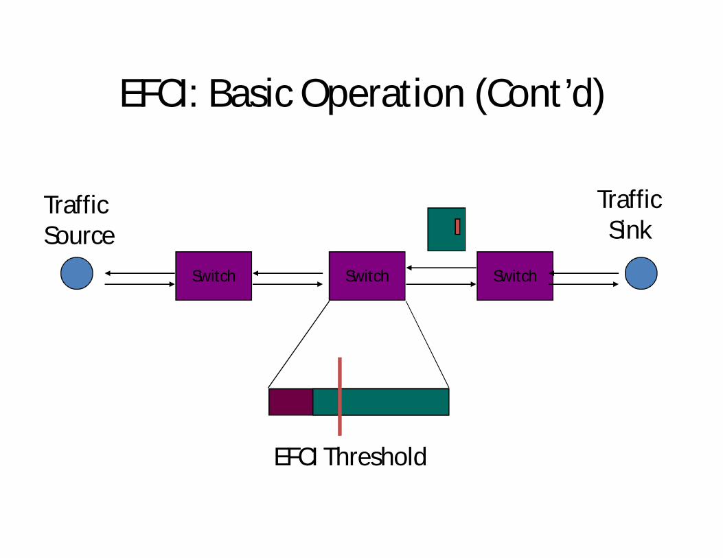
EFCI: Basic Operation (Cont’d)
Traffic Source
Traffic Sink
Switch Switch Switch
EFCI Threshold
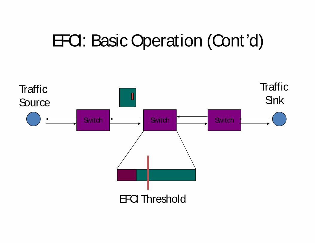
EFCI: Basic Operation (Cont’d)
Traffic Source
Traffic Sink
Switch Switch Switch
EFCI Threshold
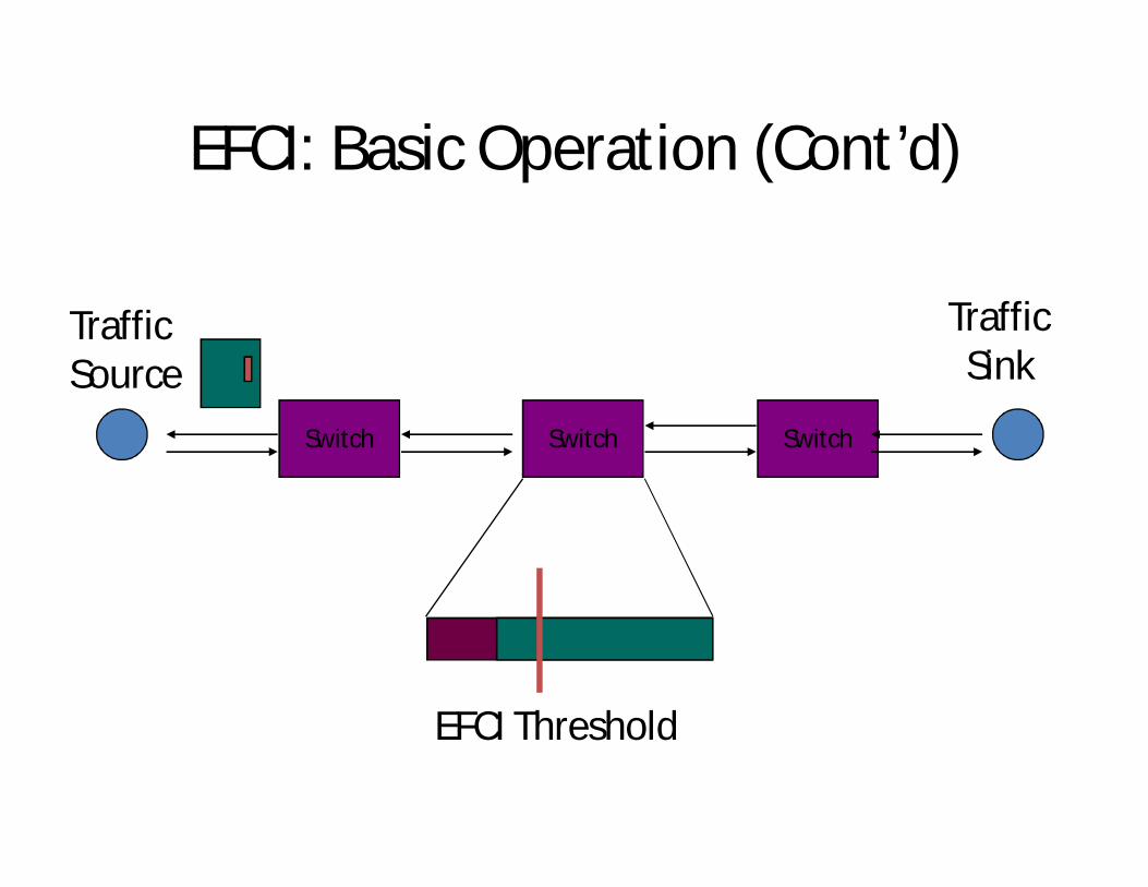
EFCI: Basic Operation (Cont’d)
Traffic Source
Traffic Sink
Switch Switch Switch
EFCI Threshold
EFCI: Basic Operation (Cont’d)
Traffic Source
Traffic Sink
Switch Switch Switch
EFCI Threshold
!!!
EFCI: Basic Operation (Cont’d)
Traffic Source
Traffic Sink
Switch Switch Switch
EFCI Threshold

EFCI: Basic Operation (Cont’d)
Traffic Source
Traffic Sink
Switch Switch Switch
EFCI Threshold

EFCI: Basic Operation (Cont’d)
Traffic Source
Traffic Sink
Switch Switch Switch
EFCI Threshold
EFCI: Basic Operation (Cont’d)
Traffic Source
Traffic Sink
Switch Switch Switch
EFCI Threshold
EFCI: Basic Operation (Cont’d)
Traffic Source
Traffic Sink
Switch Switch Switch
EFCI Threshold
UNIT V -NETWORK PERFORMANCE MODELING
AND ESTIMATION
Queuing Analysis
• Elements of Waiting Line Analysis
• The Single-Server Waiting Line System
• Undefined and Constant Service Times
• Finite Queue Length
• Finite Calling Problem
• The Multiple-Server Waiting Line
• Additional Types of Queuing Systems
Queuing AnalysisOverview
• Significant amount of time spent in waiting lines by people, products, etc.
• Providing quick service is an important aspect of quality customer service.
• The basis of waiting line analysis is the trade-off between the cost of improving service and the costs associated with making customers wait.
• Queuing analysis is a probabilistic form of analysis.
• The results are referred to as operating characteristics.
• Results are used by managers of queuing operations to make decisions.
Queuing AnalysisElements of Waiting Line Analysis
• Waiting lines form because people or things arrive at a service faster than they can be served.
• Most operations have sufficient server capacity to handle customers in the long run..
• Customers however, do not arrive at a constant rate nor are they served in an equal amount of time.
• Waiting lines are continually increasing and decreasing in length.and approach an average rate of customer arrivals and an average service time, in the long run.
• Decisions concerning the management of waiting lines are based on these averages for customer arrivals and service times.
• They are used in formulas to compute operating characteristics of the system which in turn form the basis of decision making.
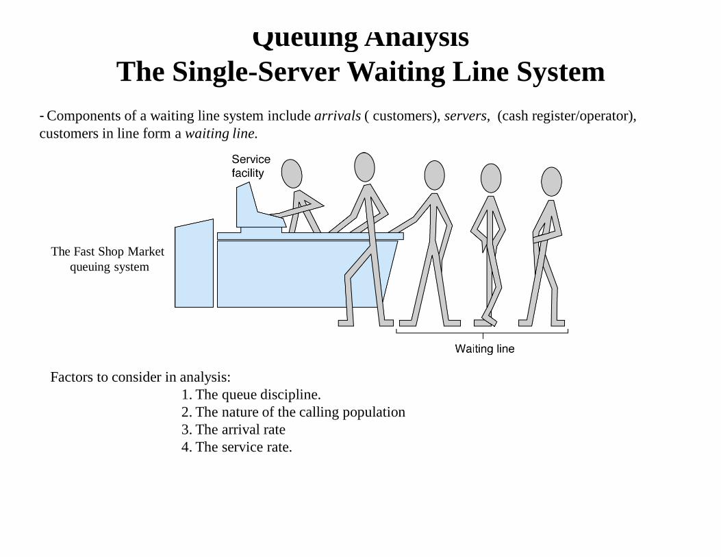
Queuing AnalysisThe Single-Server Waiting Line System
- Components of a waiting line system include arrivals ( customers), servers, (cash register/operator), customers in line form a waiting line.
Factors to consider in analysis: 1. The queue discipline.2. The nature of the calling population3. The arrival rate4. The service rate.
The Fast Shop Market queuing system
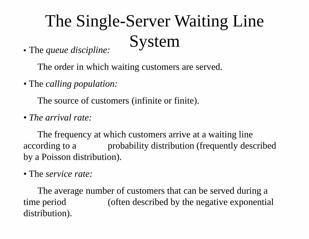
The Single-Server Waiting Line System
• The queue discipline:
The order in which waiting customers are served.
• The calling population:
The source of customers (infinite or finite).
• The arrival rate:
The frequency at which customers arrive at a waiting line according to a probability distribution (frequently described by a Poisson distribution).
• The service rate:
The average number of customers that can be served during a time period (often described by the negative exponential distribution).
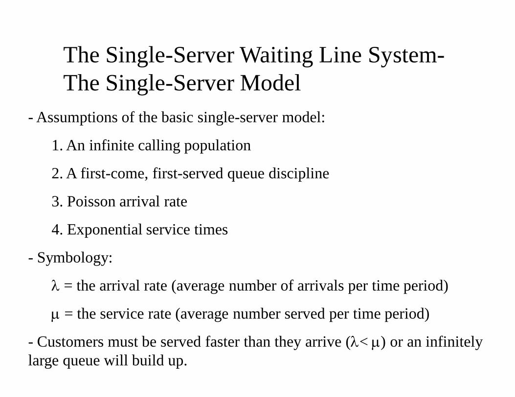
The Single-Server Waiting Line System-The Single-Server Model
- Assumptions of the basic single-server model:
1. An infinite calling population
2. A first-come, first-served queue discipline
3. Poisson arrival rate
4. Exponential service times
- Symbology:
= the arrival rate (average number of arrivals per time period)
= the service rate (average number served per time period)
- Customers must be served faster than they arrive (< ) or an infinitely large queue will build up.
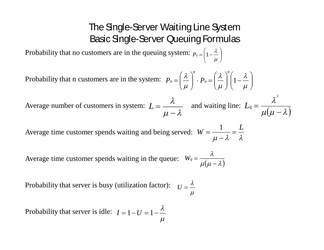
The Single-Server Waiting Line SystemBasic Single-Server Queuing Formulas
Probability that no customers are in the queuing system:
Probability that n customers are in the system:
Average number of customers in system: and waiting line:
Average time customer spends waiting and being served:
Average time customer spends waiting in the queue:
Probability that server is busy (utilization factor):
Probability that server is idle:
1oP
1
n
o
n
n PP
2
qL
LW
1
qW
U
11 UI
L
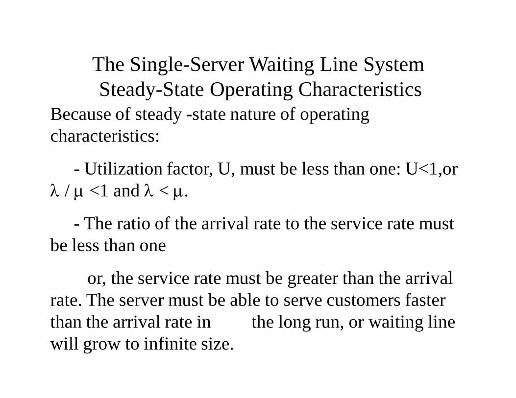
The Single-Server Waiting Line SystemSteady-State Operating Characteristics
Because of steady -state nature of operating characteristics:
- Utilization factor, U, must be less than one: U<1,or / <1 and < .
- The ratio of the arrival rate to the service rate must be less than one
or, the service rate must be greater than the arrival rate. The server must be able to serve customers faster than the arrival rate in the long run, or waiting line will grow to infinite size.
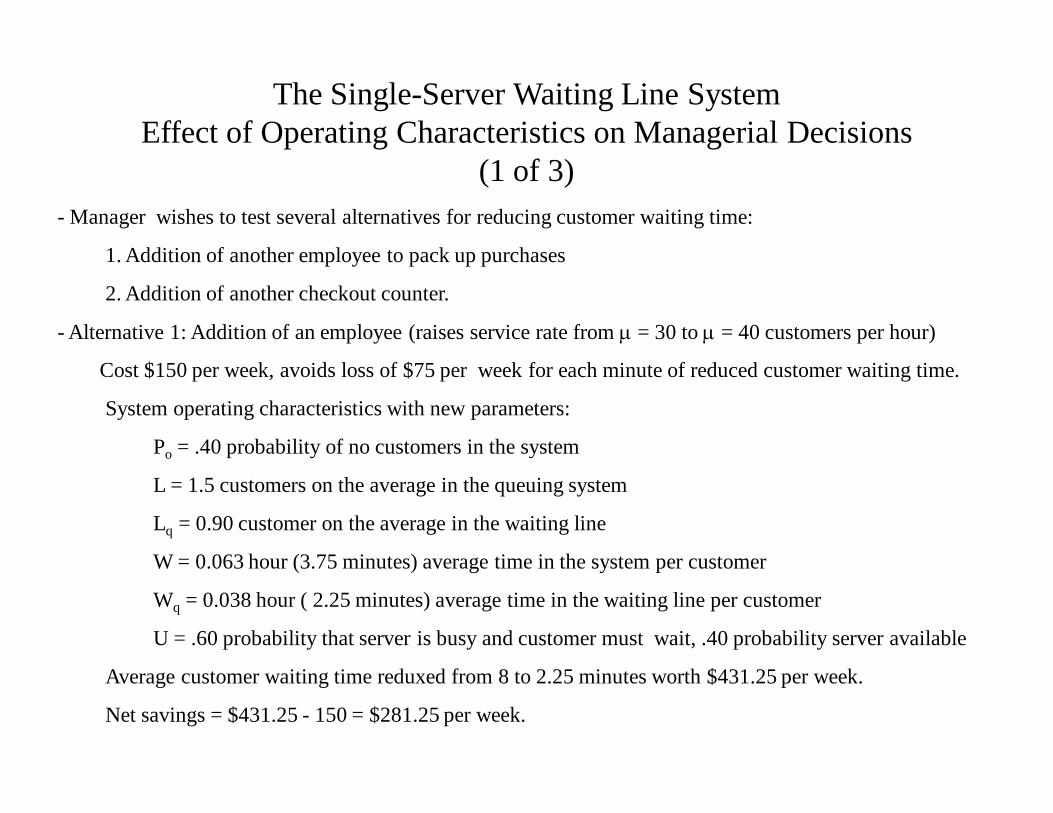
The Single-Server Waiting Line SystemEffect of Operating Characteristics on Managerial Decisions
(1 of 3)- Manager wishes to test several alternatives for reducing customer waiting time:
1. Addition of another employee to pack up purchases
2. Addition of another checkout counter.
- Alternative 1: Addition of an employee (raises service rate from = 30 to = 40 customers per hour)
Cost $150 per week, avoids loss of $75 per week for each minute of reduced customer waiting time.
System operating characteristics with new parameters:
Po = .40 probability of no customers in the system
L = 1.5 customers on the average in the queuing system
Lq = 0.90 customer on the average in the waiting line
W = 0.063 hour (3.75 minutes) average time in the system per customer
Wq = 0.038 hour ( 2.25 minutes) average time in the waiting line per customer
U = .60 probability that server is busy and customer must wait, .40 probability server available
Average customer waiting time reduxed from 8 to 2.25 minutes worth $431.25 per week.
Net savings = $431.25 - 150 = $281.25 per week.
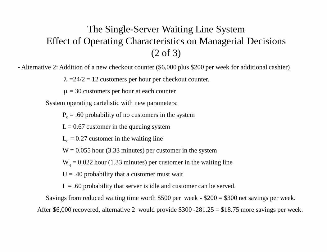
The Single-Server Waiting Line SystemEffect of Operating Characteristics on Managerial Decisions
(2 of 3)- Alternative 2: Addition of a new checkout counter ($6,000 plus $200 per week for additional cashier)
=24/2 = 12 customers per hour per checkout counter.
= 30 customers per hour at each counter
System operating cartelistic with new parameters:
Po = .60 probability of no customers in the system
L = 0.67 customer in the queuing system
Lq = 0.27 customer in the waiting line
W = 0.055 hour (3.33 minutes) per customer in the system
Wq = 0.022 hour (1.33 minutes) per customer in the waiting line
U = .40 probability that a customer must wait
I = .60 probability that server is idle and customer can be served.
Savings from reduced waiting time worth $500 per week - $200 = $300 net savings per week.
After $6,000 recovered, alternative 2 would provide $300 -281.25 = $18.75 more savings per week.
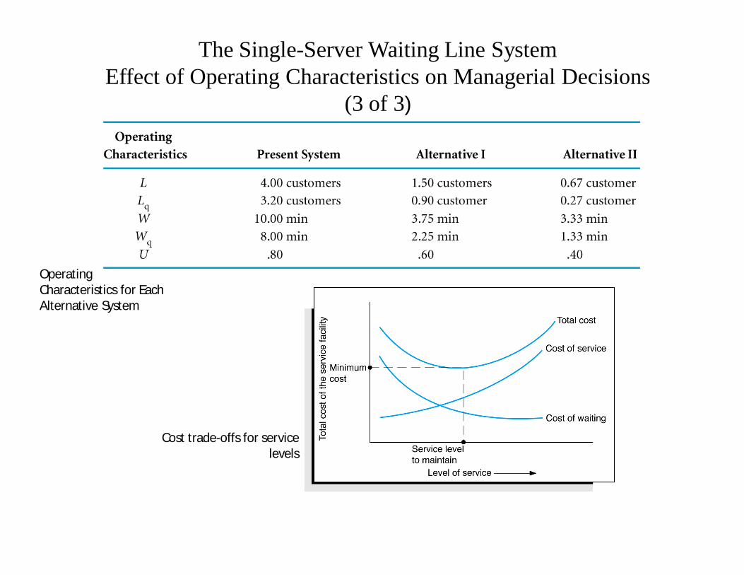
The Single-Server Waiting Line SystemEffect of Operating Characteristics on Managerial Decisions
(3 of 3)
Operating Characteristics for Each Alternative System
Cost trade-offs for service levels
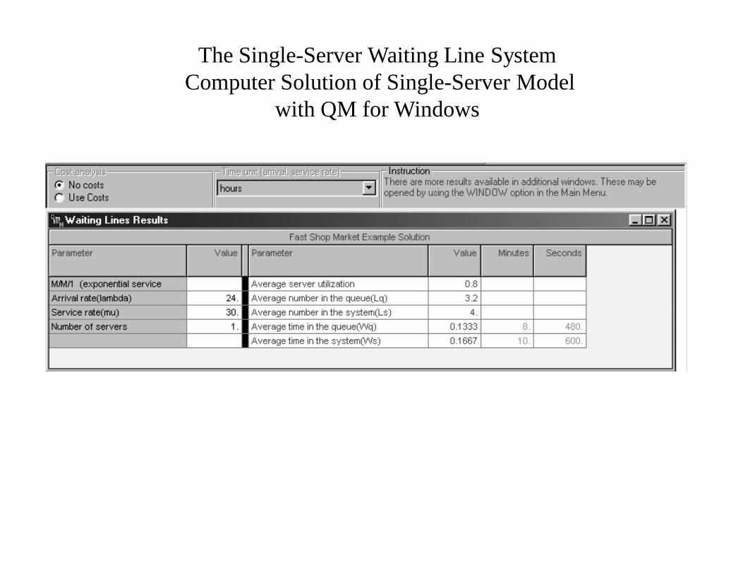
The Single-Server Waiting Line SystemComputer Solution of Single-Server Model
with QM for Windows
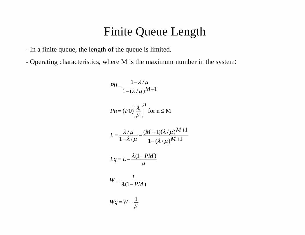
Finite Queue Length- In a finite queue, the length of the queue is limited.
- Operating characteristics, where M is the maximum number in the system:
1
)1(
)1(
1)/(1
1)/)(1(/1
/
M n for )0(
1)/(1/10
WWq
PMLW
PMLLq
MMML
nPPn
MP
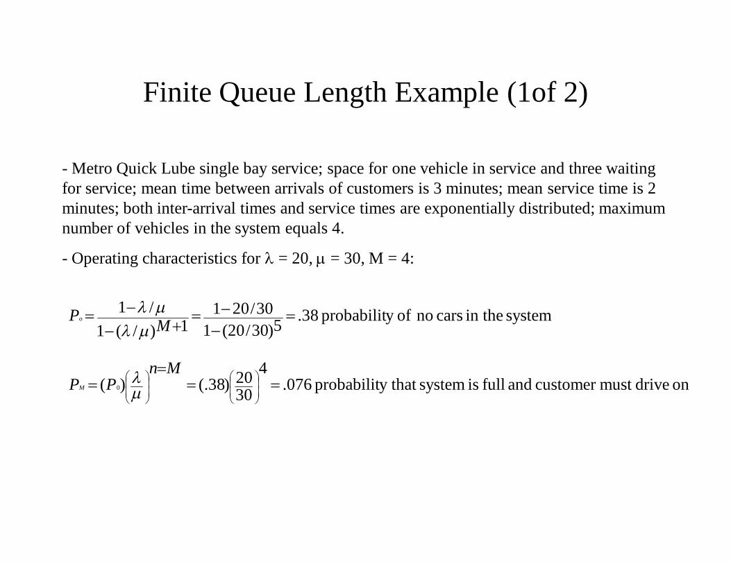
Finite Queue Length Example (1of 2)
- Metro Quick Lube single bay service; space for one vehicle in service and three waiting for service; mean time between arrivals of customers is 3 minutes; mean service time is 2 minutes; both inter-arrival times and service times are exponentially distributed; maximum number of vehicles in the system equals 4.
- Operating characteristics for = 20, = 30, M = 4:
on drivemust customer and full is systemy that probabilit .076 4
3020)38(.)(
system in the cars no ofy probabilit .38 5)30/20(130/201
1)/(1/1
0
Mn
PP
MP
M
o
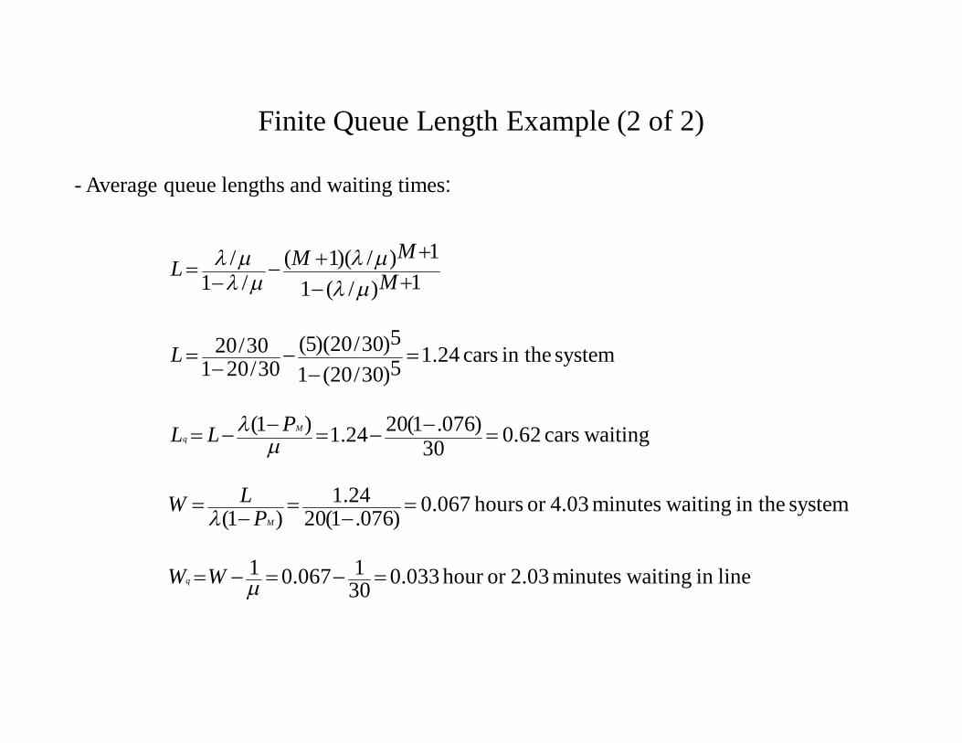
Finite Queue Length Example (2 of 2)
- Average queue lengths and waiting times:
linein waitingminutes 2.03or hour 0.033301067.01
system in the waitingminutes 4.03or hours 0.067 )076.1(2024.1
)1(
waitingcars 0.62 30)076.1(2024.1)1(
system in the cars 1.24 5)30/20(1
5)30/20)(5(30/201
30/20
1)/(1
1)/)(1(/1
/
WW
PLW
PLL
L
MMML
q
M
Mq
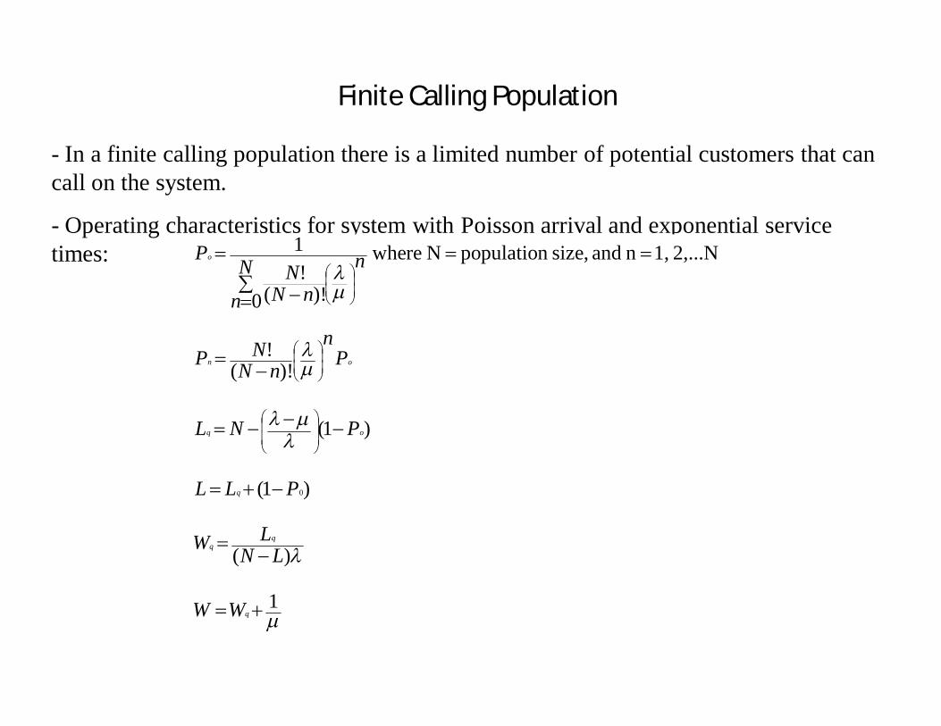
Finite Calling Population
- In a finite calling population there is a limited number of potential customers that can call on the system.
- Operating characteristics for system with Poisson arrival and exponential service times:
1
)(
)1(
)1(
)!(!
2,...N 1, n and size, population N where
0 )!(!
1
0
q
q
oq
on
o
WW
LNLW
PLL
PNL
Pn
nNNP
nN
n nNN
P
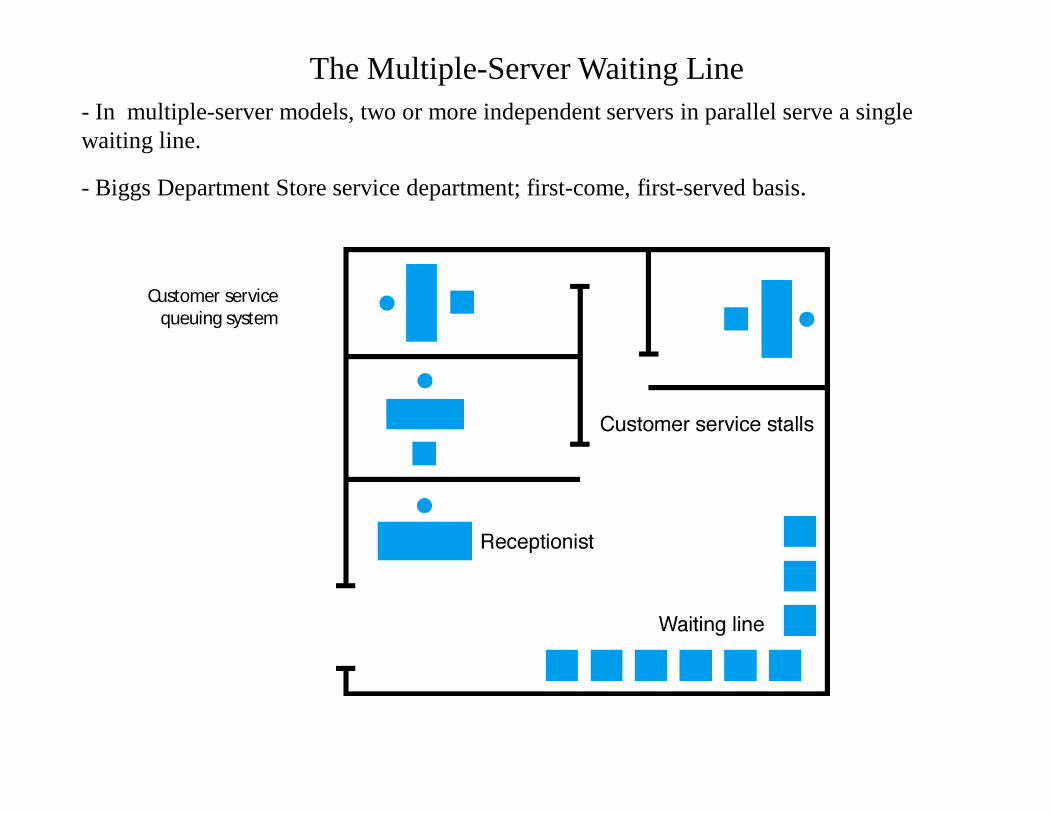
The Multiple-Server Waiting Line- In multiple-server models, two or more independent servers in parallel serve a single waiting line.
- Biggs Department Store service department; first-come, first-served basis.
Customer service queuing system
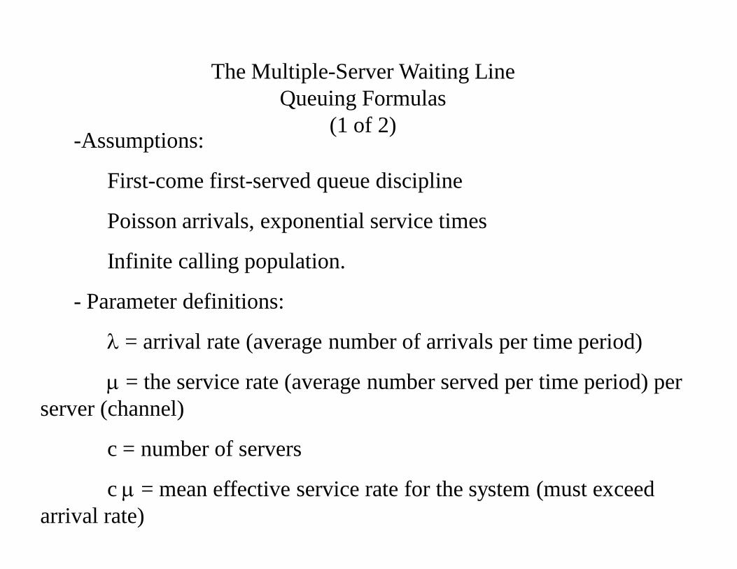
The Multiple-Server Waiting LineQueuing Formulas
(1 of 2) -Assumptions:
First-come first-served queue discipline
Poisson arrivals, exponential service times
Infinite calling population.
- Parameter definitions:
= arrival rate (average number of arrivals per time period)
= the service rate (average number served per time period) per server (channel)
c = number of servers
c = mean effective service rate for the system (must exceed arrival rate)
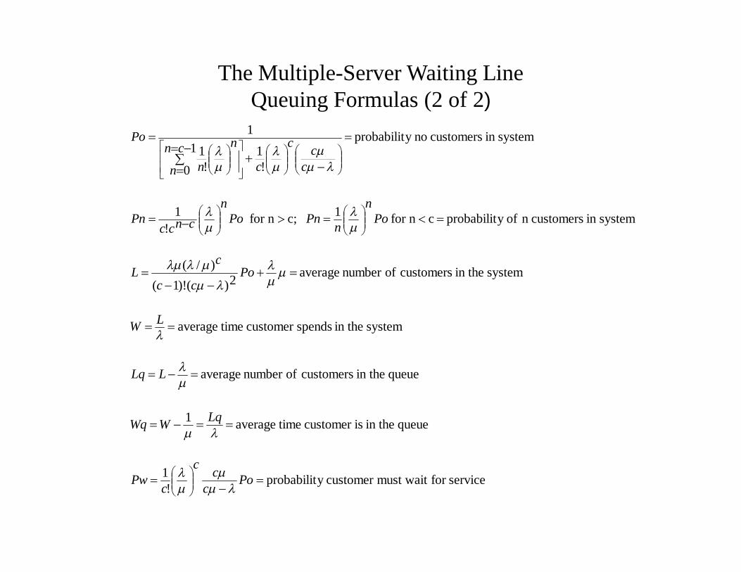
The Multiple-Server Waiting LineQueuing Formulas (2 of 2)
servicefor must wait customer y probabilit !
1
queue in the iscustomer timeaverage 1
queue in the customers ofnumber average
system in the spendscustomer timeaverage
system in the customers ofnumber average 2)()!1()/(
systemin customersn ofy probabilit c nfor 1 c;nfor !
1
systemin customers noy probabilit
!11
0 !1
1
Poc
cc
cPw
LqWWq
LLq
LW
Pocc
cL
Pon
nPnPo
ncncc
Pn
ccc
ccn
n
n
n
Po
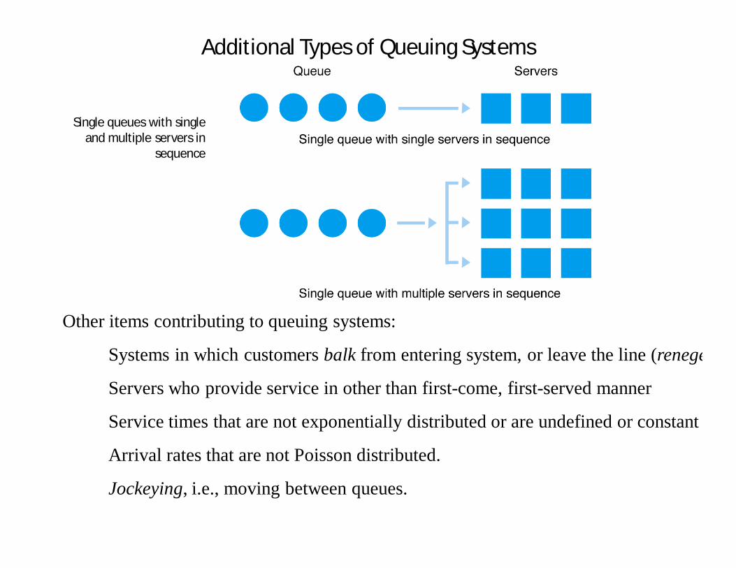
Additional Types of Queuing Systems
Other items contributing to queuing systems:
Systems in which customers balk from entering system, or leave the line (renege).
Servers who provide service in other than first-come, first-served manner
Service times that are not exponentially distributed or are undefined or constant
Arrival rates that are not Poisson distributed.
Jockeying, i.e., moving between queues.
Single queues with single and multiple servers in
sequence
Queuing analysis-Queuing System Concepts Arrival Rate, Occupancy, Time in the System
• Queuing system – Data network where packets arrive, wait in
various queues, receive service at various points, and exit after some time
• Arrival rate– Long-term number of arrivals per unit time
• Occupancy– Number of packets in the system (averaged over a
long time)• Time in the system (delay)
– Time from packet entry to exit (averaged over many packets)
Stability and Steady-State• A single queue system is stable if
packet arrival rate < system transmission capacity• For a single queue, the ratio
packet arrival rate / system transmission capacityis called the utilization factor– Describes the loading of a queue
• In an unstable system packets accumulate in various queues and/or get dropped
• For unstable systems with large buffers some packet delays become very large– Flow/admission control may be used to limit the packet
arrival rate– Prioritization of flows keeps delays bounded for the
important traffic
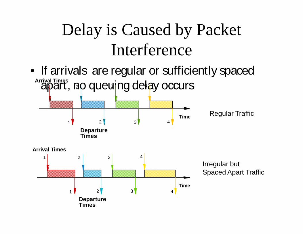
Delay is Caused by Packet Interference
• If arrivals are regular or sufficiently spaced apart, no queuing delay occurs
Regular Traffic
Irregular but Spaced Apart Traffic
Time
Arrival Times
Departure Times
1 3 42
1 3 42
Time
Arrival Times
Departure Times
1 3 42
1 3 42
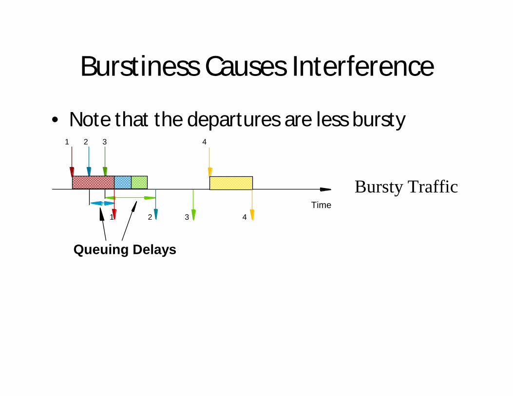
Burstiness Causes Interference
• Note that the departures are less bursty
Time
Queuing Delays
Bursty Traffic
1 2 3 4
1 2 3 4
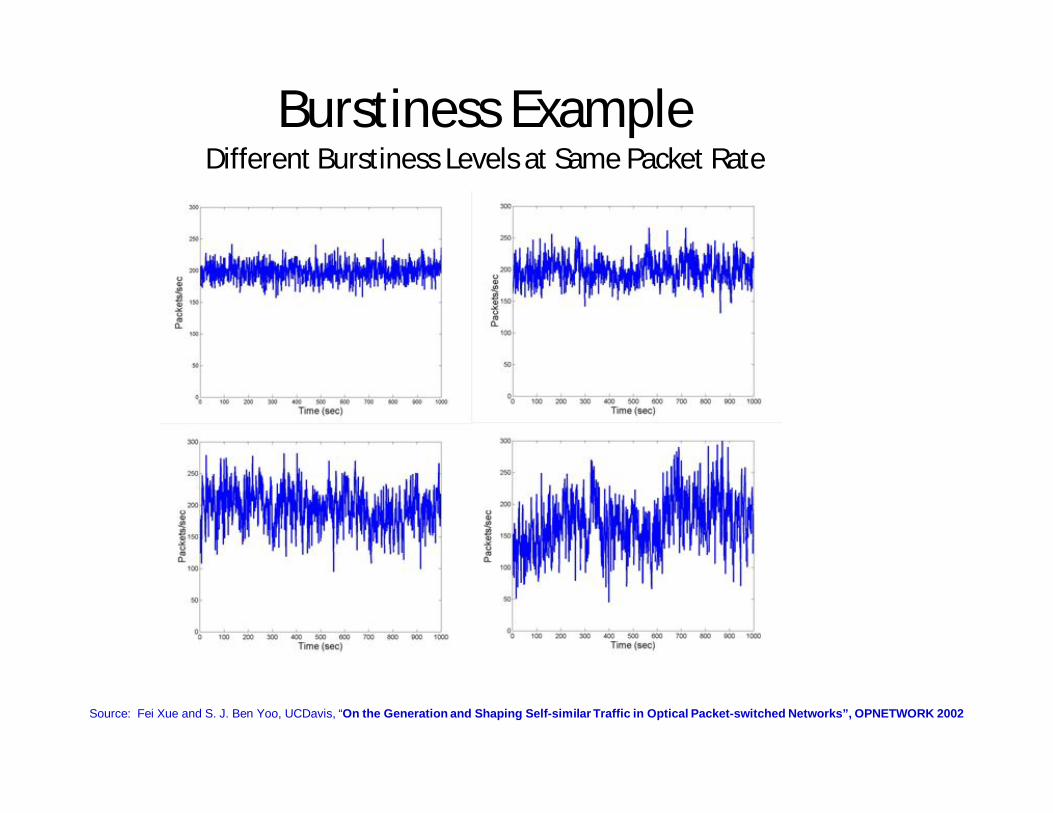
Burstiness ExampleDifferent Burstiness Levels at Same Packet Rate
Source: Fei Xue and S. J. Ben Yoo, UCDavis, “On the Generation and Shaping Self-similar Traffic in Optical Packet-switched Networks”, OPNETWORK 2002
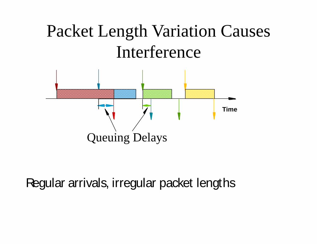
Packet Length Variation Causes Interference
Regular arrivals, irregular packet lengths
Time
Queuing Delays
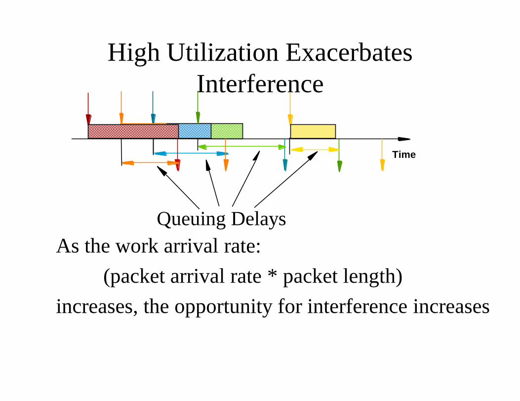
High Utilization Exacerbates Interference
As the work arrival rate: (packet arrival rate * packet length)
increases, the opportunity for interference increases
Time
Queuing Delays
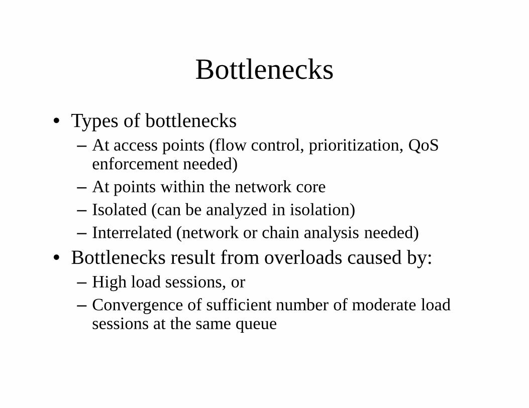
Bottlenecks
• Types of bottlenecks– At access points (flow control, prioritization, QoS
enforcement needed)– At points within the network core– Isolated (can be analyzed in isolation)– Interrelated (network or chain analysis needed)
• Bottlenecks result from overloads caused by: – High load sessions, or – Convergence of sufficient number of moderate load
sessions at the same queue
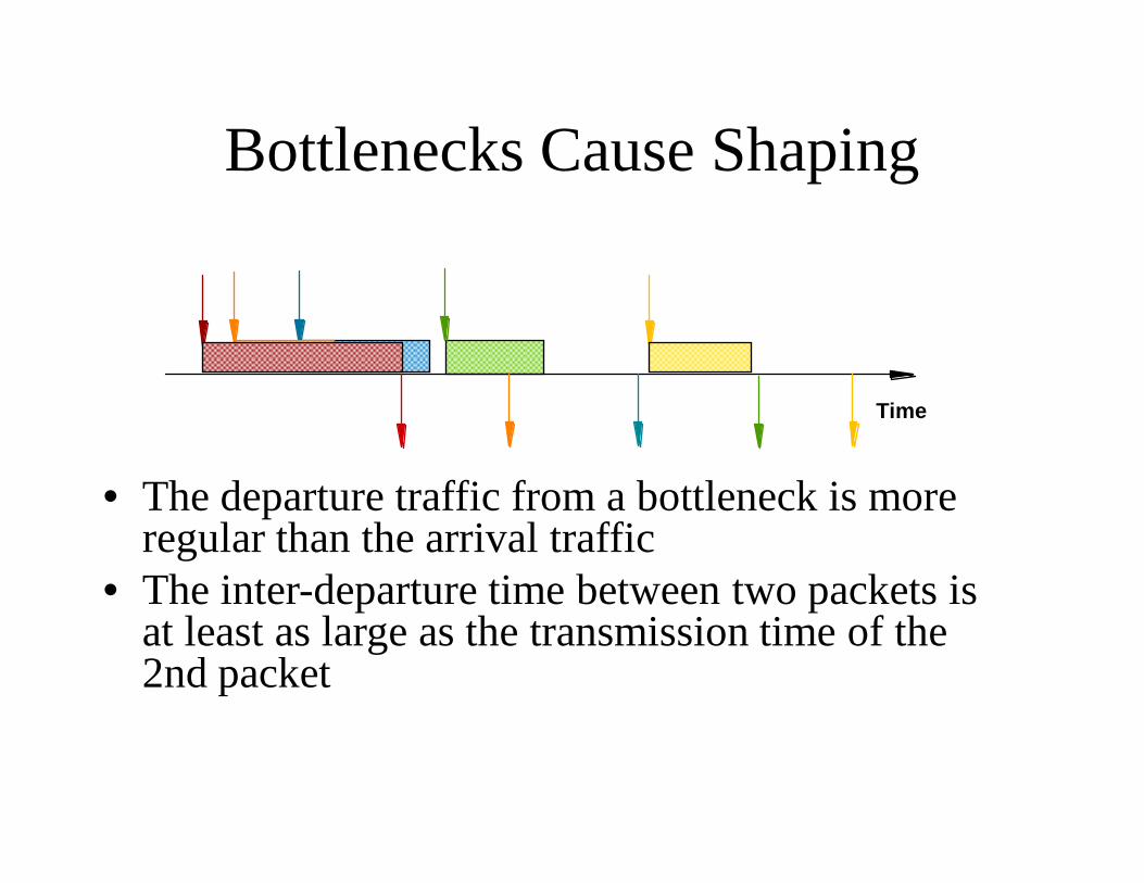
Bottlenecks Cause Shaping
• The departure traffic from a bottleneck is more regular than the arrival traffic
• The inter-departure time between two packets is at least as large as the transmission time of the 2nd packet
Time
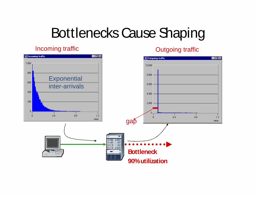
Bottlenecks Cause Shaping
Bottleneck 90% utilization
Outgoing trafficIncoming traffic
Exponentialinter-arrivals
gap
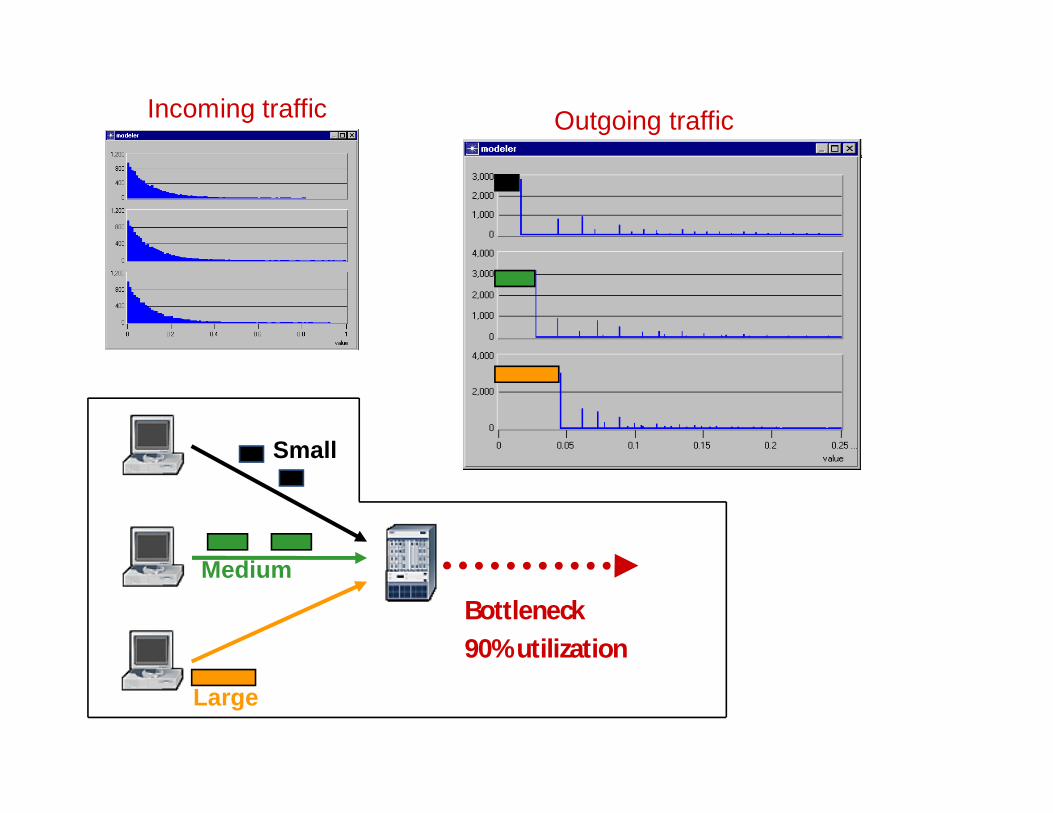
Bottleneck 90% utilization
Outgoing trafficIncoming traffic
Large
Medium
Small
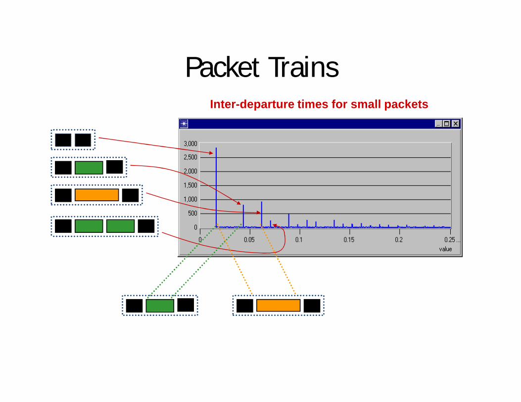
Packet TrainsInter-departure times for small packets
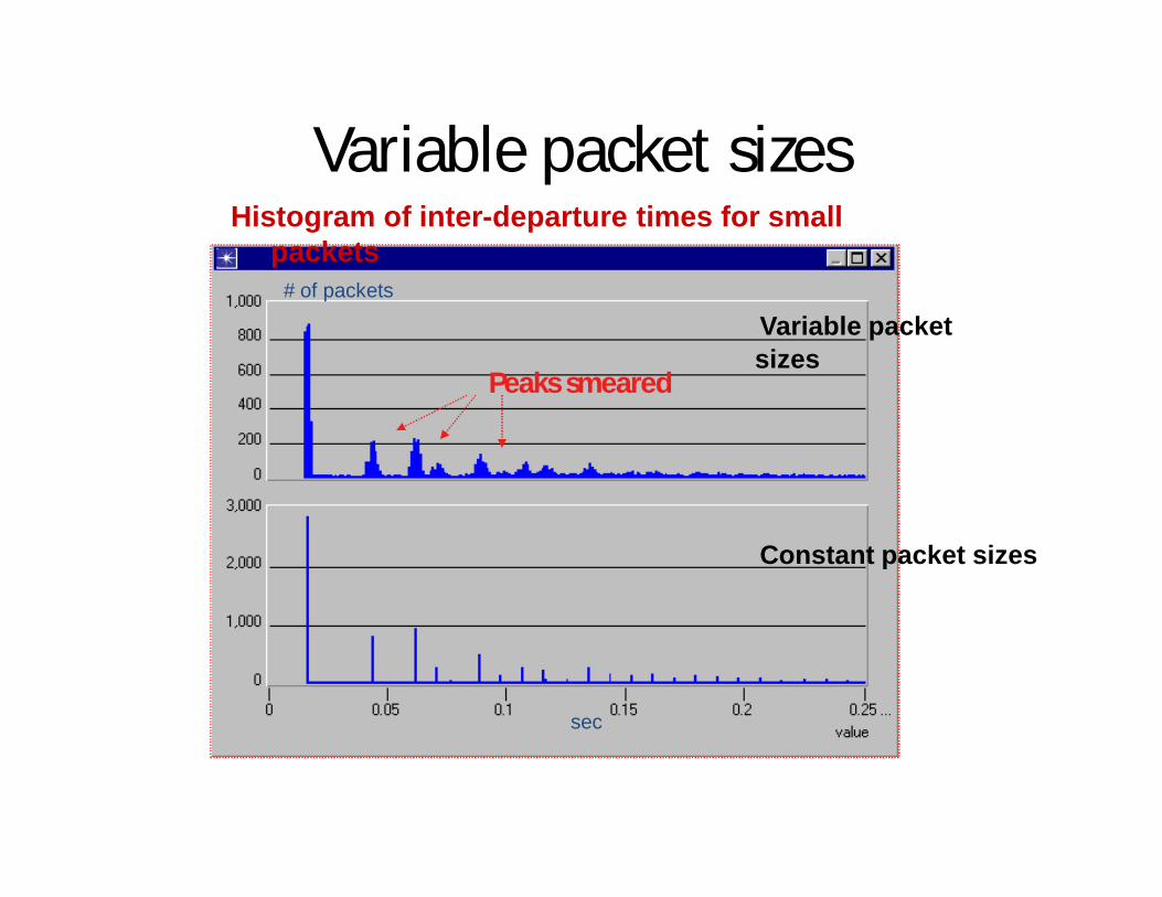
Variable packet sizesHistogram of inter-departure times for small
packets
sec
# of packets
Peaks smeared
Variable packet sizes
Constant packet sizes
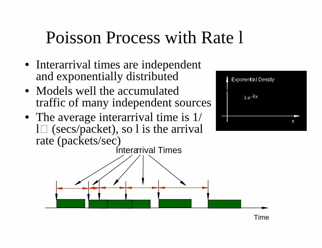
Poisson Process with Rate l• Interarrival times are independent
and exponentially distributed• Models well the accumulated
traffic of many independent sources• The average interarrival time is 1/
l (secs/packet), so l is the arrival rate (packets/sec)
Time
Interarrival Times
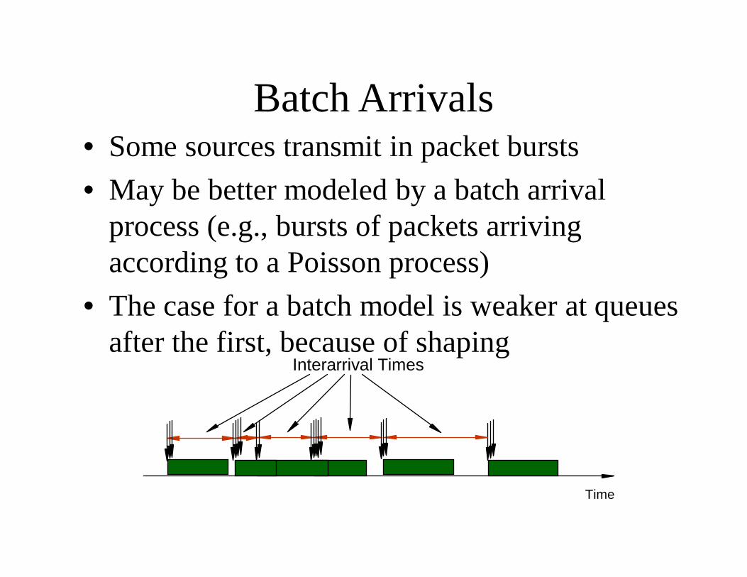
Batch Arrivals• Some sources transmit in packet bursts • May be better modeled by a batch arrival
process (e.g., bursts of packets arriving according to a Poisson process)
• The case for a batch model is weaker at queues after the first, because of shaping
Time
Interarrival Times
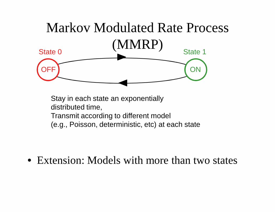
Markov Modulated Rate Process (MMRP)
• Extension: Models with more than two states
Stay in each state an exponentially distributed time, Transmit according to different model (e.g., Poisson, deterministic, etc) at each state
State 0 State 1
OFF ON
Source Types
• Voice sources• Video sources• File transfers• Web traffic• Interactive traffic• Different application types have different QoS
requirements, e.g., delay, jitter, loss, throughput, etc.
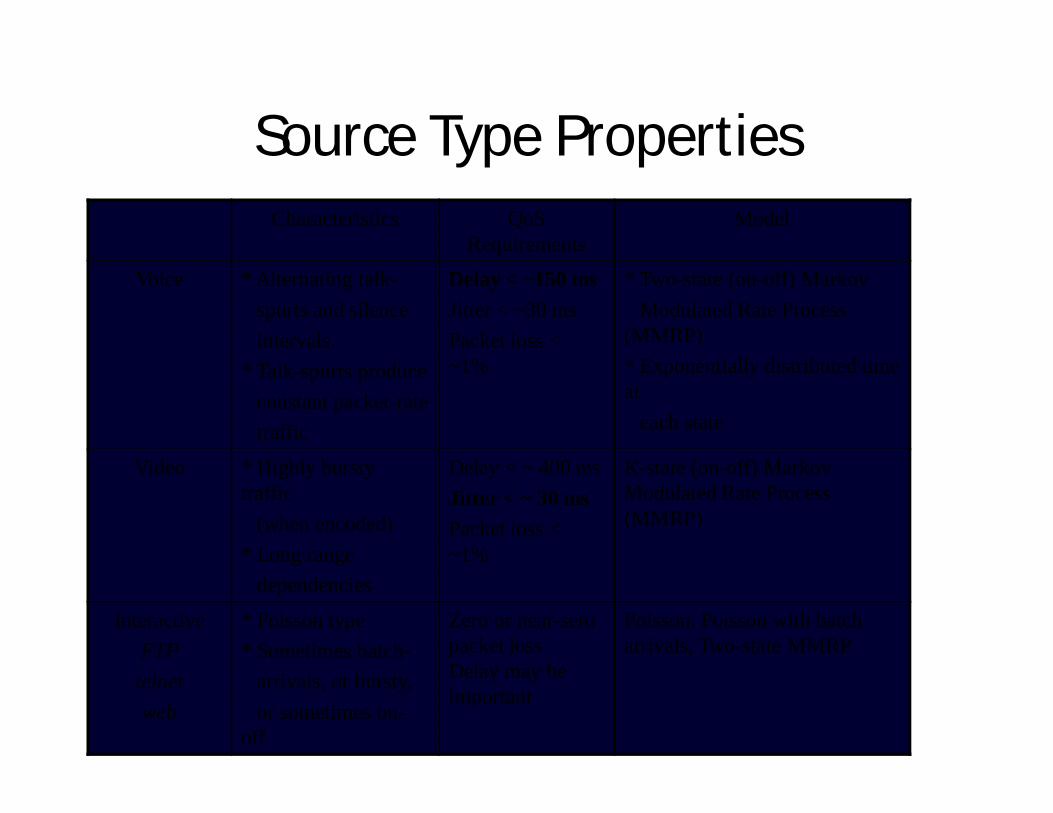
Source Type Properties Characteristics QoS
RequirementsModel
Voice * Alternating talk-spurts and silence intervals.
* Talk-spurts produce constant packet-rate traffic
Delay < ~150 msJitter < ~30 msPacket loss < ~1%
* Two-state (on-off) Markov Modulated Rate Process
(MMRP)* Exponentially distributed time at
each state
Video * Highly bursty traffic
(when encoded)* Long range
dependencies
Delay < ~ 400 msJitter < ~ 30 msPacket loss < ~1%
K-state (on-off) Markov Modulated Rate Process (MMRP)
InteractiveFTPtelnetweb
* Poisson type * Sometimes batch-
arrivals, or bursty, or sometimes on-
off
Zero or near-sero packet loss Delay may be important
Poisson, Poisson with batch arrivals, Two-state MMRP
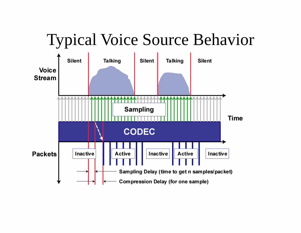
Typical Voice Source Behavior
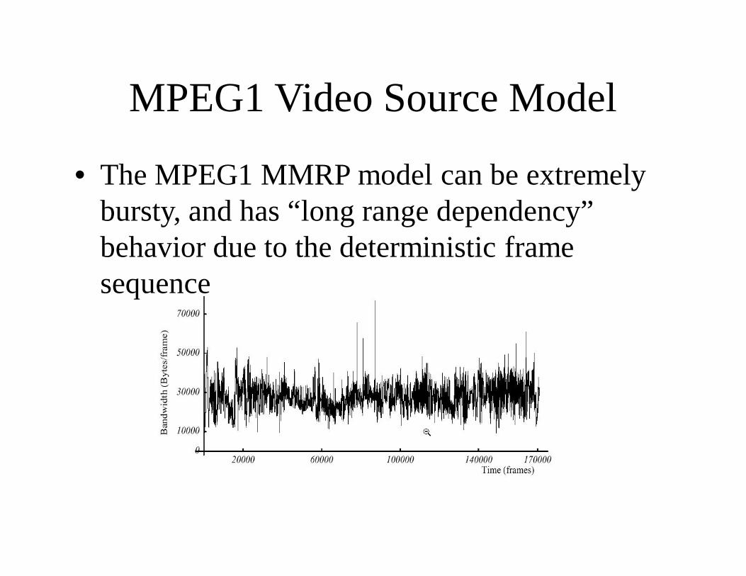
MPEG1 Video Source Model
• The MPEG1 MMRP model can be extremely bursty, and has “long range dependency” behavior due to the deterministic frame sequence
Device Queuing Mechanisms• Common queue examples for IP routers
– FIFO: First In First Out– PQ: Priority Queuing– WFQ: Weighted Fair Queuing– Combinations of the above
• Service types from a queuing theory standpoint– Single server (one queue - one transmission line)– Multiple server (one queue - several transmission lines)– Priority server (several queues with hard priorities - one
transmission line)– Shared server (several queues with soft priorities - one
transmission line)
Single Server FIFO
• Single transmission line serving packets on a FIFO (First-In-First-Out) basis
• Each packet must wait for all packets found in the system to complete transmission, before starting transmission– Departure Time = Arrival Time + Workload Found
in the System +Transmission time• Packets arriving to a full buffer are dropped
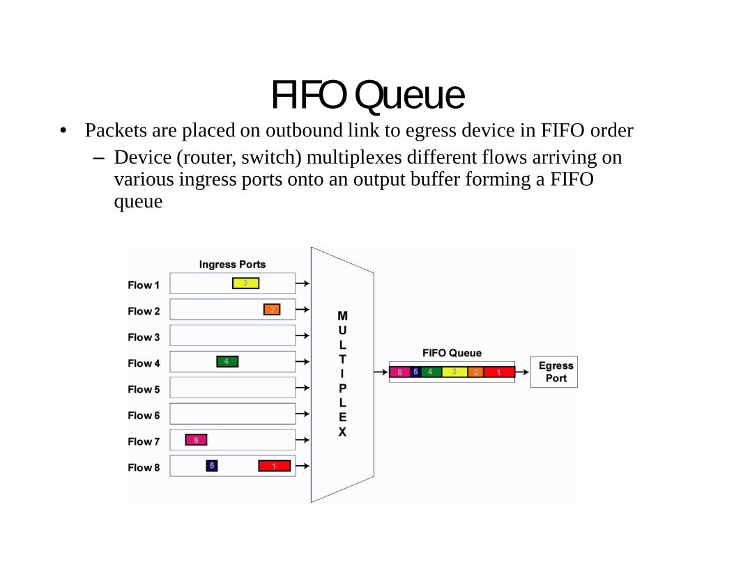
FIFO Queue• Packets are placed on outbound link to egress device in FIFO order
– Device (router, switch) multiplexes different flows arriving on various ingress ports onto an output buffer forming a FIFO queue
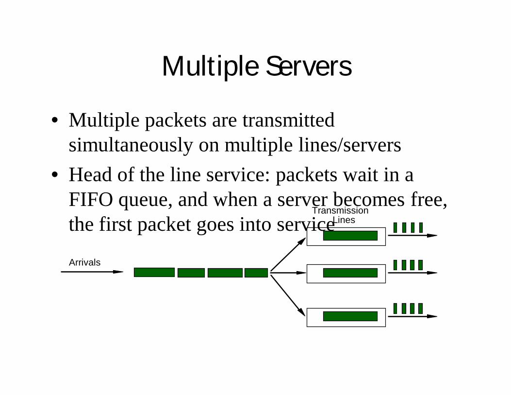
Multiple Servers
• Multiple packets are transmitted simultaneously on multiple lines/servers
• Head of the line service: packets wait in a FIFO queue, and when a server becomes free, the first packet goes into service
Arrivals
Transmission Lines
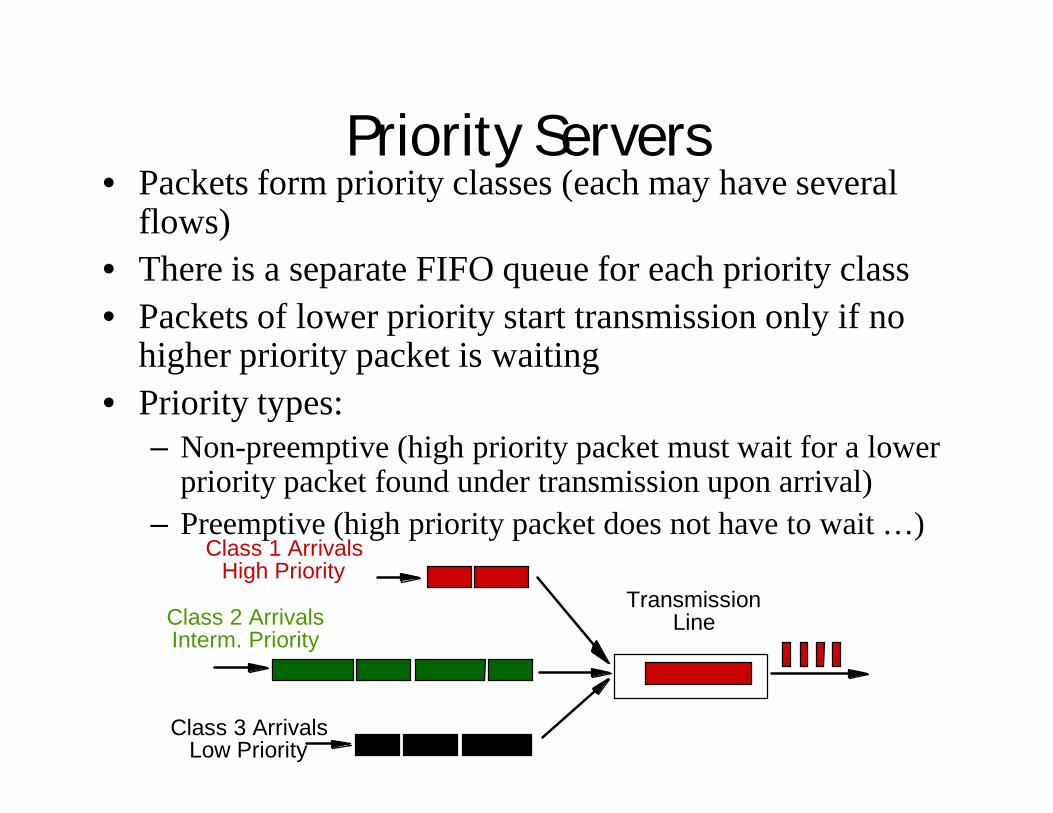
Priority Servers• Packets form priority classes (each may have several
flows)• There is a separate FIFO queue for each priority class• Packets of lower priority start transmission only if no
higher priority packet is waiting• Priority types:
– Non-preemptive (high priority packet must wait for a lower priority packet found under transmission upon arrival)
– Preemptive (high priority packet does not have to wait …)Class 1 Arrivals
High PriorityTransmission
Line
Class 3 Arrivals Low Priority
Class 2 Arrivals Interm. Priority
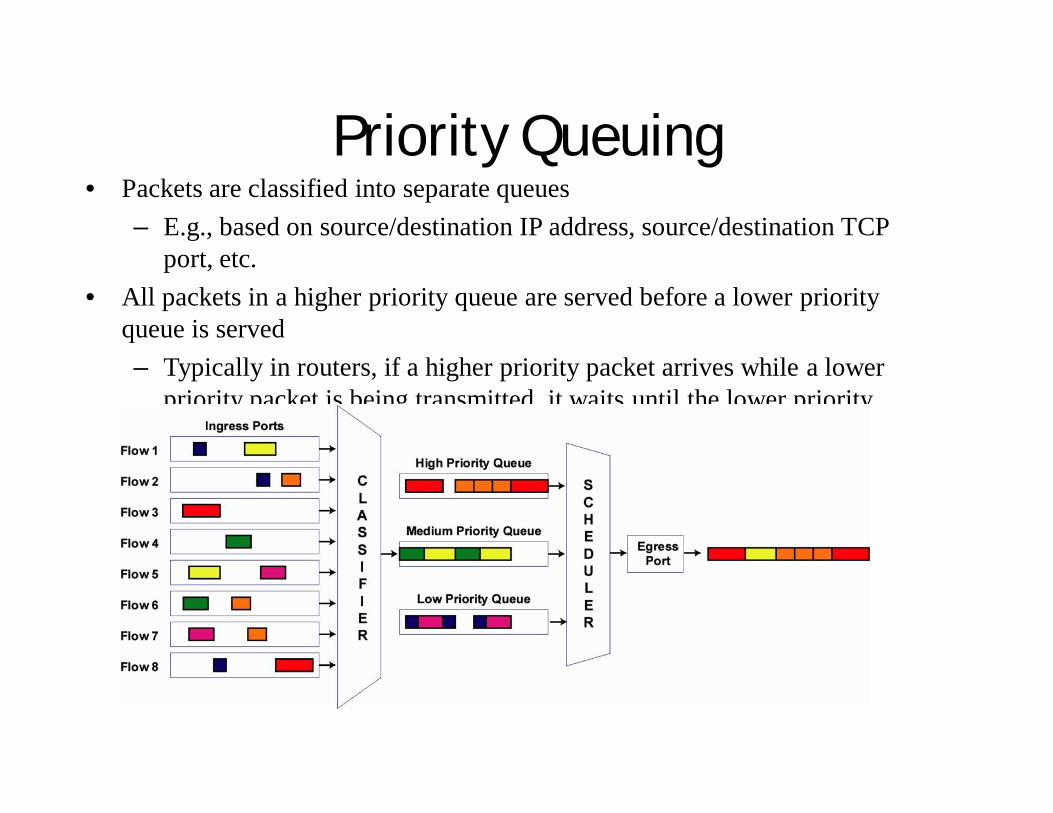
Priority Queuing• Packets are classified into separate queues
– E.g., based on source/destination IP address, source/destination TCP port, etc.
• All packets in a higher priority queue are served before a lower priority queue is served– Typically in routers, if a higher priority packet arrives while a lower
priority packet is being transmitted, it waits until the lower priority packet completes
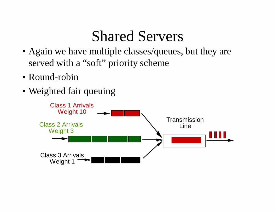
Shared Servers• Again we have multiple classes/queues, but they are
served with a “soft” priority scheme• Round-robin• Weighted fair queuing
Class 1 Arrivals Weight 10
Transmission Line
Class 3 Arrivals Weight 1
Class 2 Arrivals Weight 3
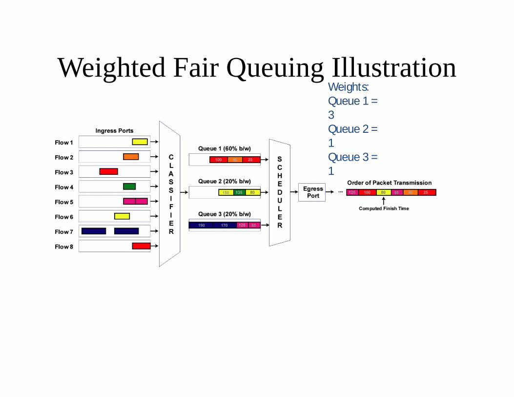
Weighted Fair Queuing IllustrationWeights:Queue 1 = 3Queue 2 = 1Queue 3 = 1
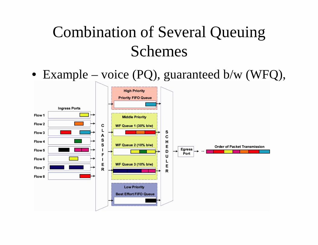
Combination of Several Queuing Schemes
• Example – voice (PQ), guaranteed b/w (WFQ), Best Effort(Cisco’s LLQ implementation)
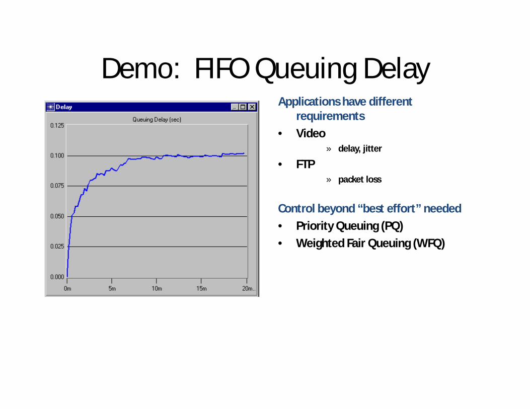
Demo: FIFO Queuing DelayApplications have different
requirements• Video
» delay, jitter
• FTP» packet loss
Control beyond “best effort” needed• Priority Queuing (PQ)• Weighted Fair Queuing (WFQ)
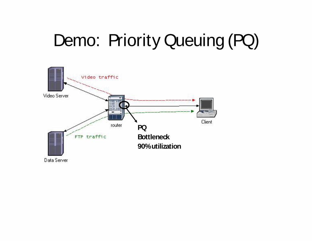
Demo: Priority Queuing (PQ)
PQBottleneck 90% utilization
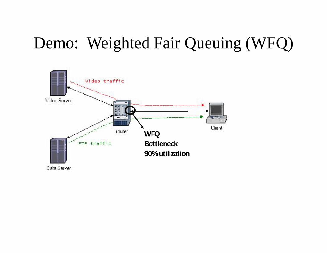
Demo: Weighted Fair Queuing (WFQ)
WFQBottleneck 90% utilization
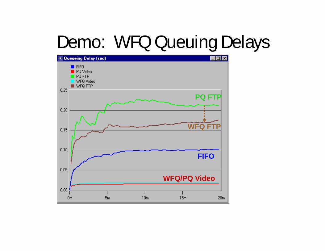
Demo: WFQ Queuing Delays
FIFO
WFQ/PQ Video
PQ FTP
WFQ FTP
Queuing: Take Away Points
• Choice of queuing mechanism can have a profound effect on performance
• To achieve desired service differentiation, appropriate queuing mechanisms can be used
• Complex queuing mechanisms may require simulation techniques to analyze behavior
• Improper configuration (e.g., queuing mechanism selection or weights) may impact performance of low priority traffic
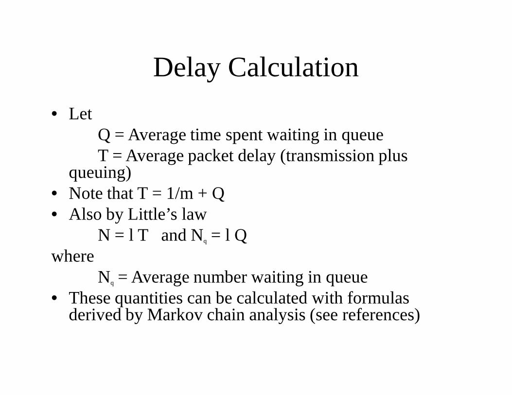
Delay Calculation• Let
Q = Average time spent waiting in queueT = Average packet delay (transmission plus
queuing) • Note that T = 1/m + Q• Also by Little’s law
N = l T and Nq = l Q where
Nq = Average number waiting in queue• These quantities can be calculated with formulas
derived by Markov chain analysis (see references)
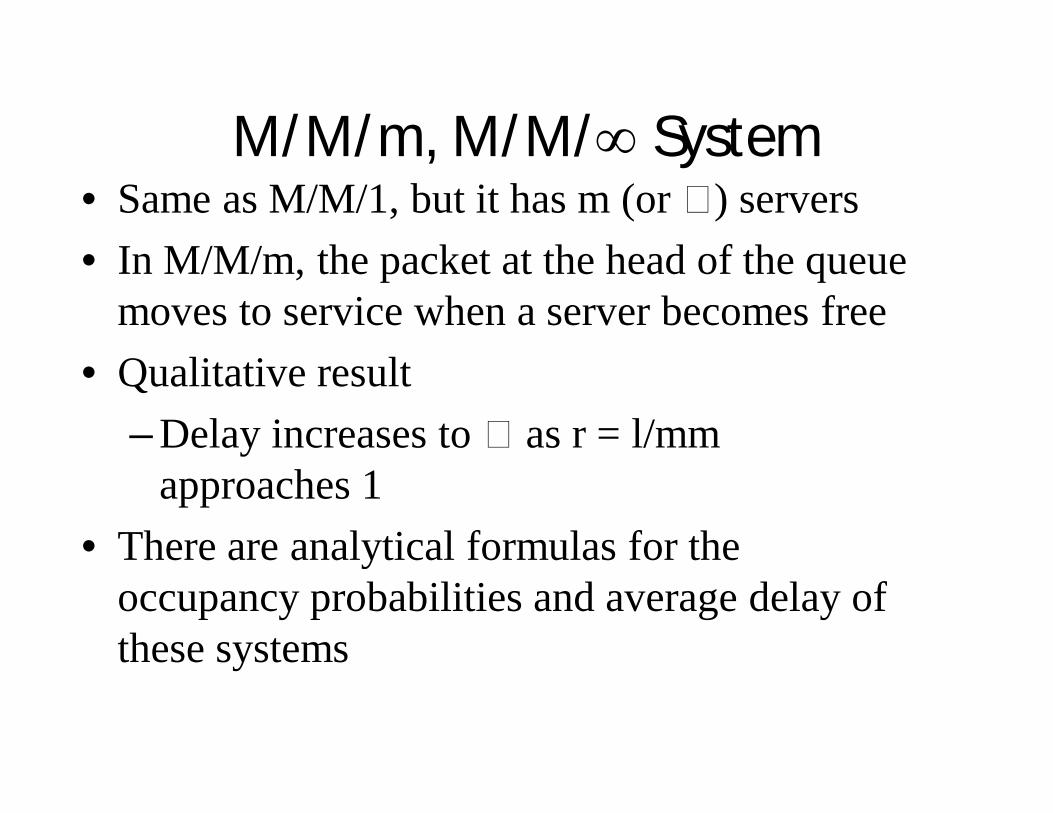
M/M/m, M/M/ System• Same as M/M/1, but it has m (or ) servers• In M/M/m, the packet at the head of the queue
moves to service when a server becomes free• Qualitative result
– Delay increases to as r = l/mm approaches 1
• There are analytical formulas for the occupancy probabilities and average delay of these systems
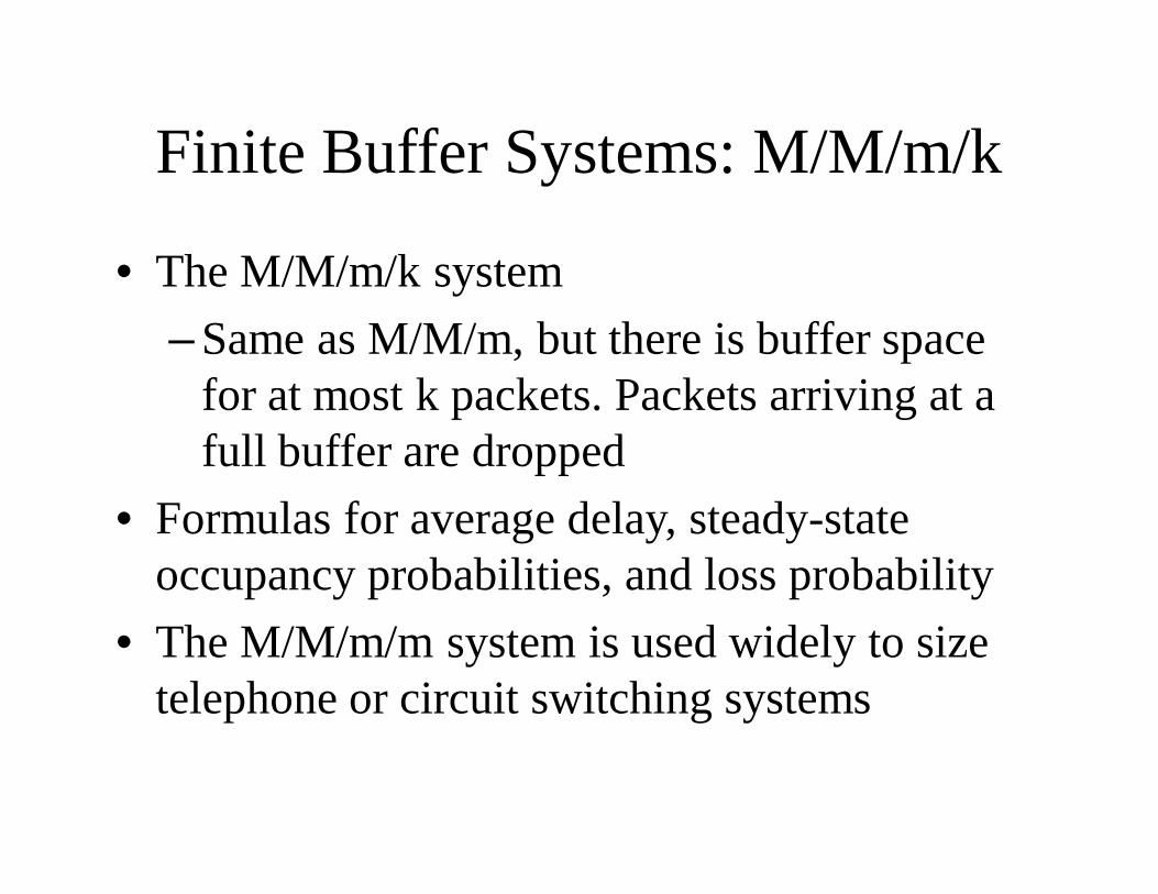
Finite Buffer Systems: M/M/m/k
• The M/M/m/k system– Same as M/M/m, but there is buffer space
for at most k packets. Packets arriving at a full buffer are dropped
• Formulas for average delay, steady-state occupancy probabilities, and loss probability
• The M/M/m/m system is used widely to size telephone or circuit switching systems
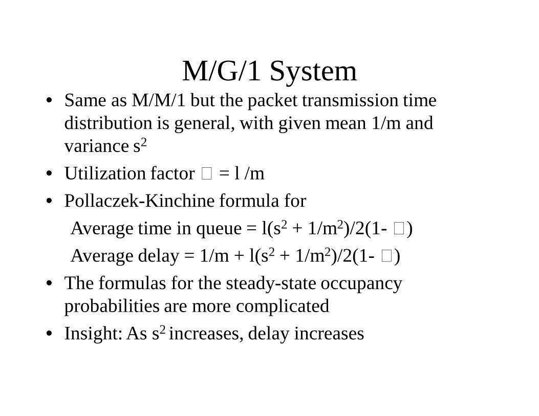
M/G/1 System• Same as M/M/1 but the packet transmission time
distribution is general, with given mean 1/m and variance s2
• Utilization factor = l /m• Pollaczek-Kinchine formula for
Average time in queue = l(s2 + 1/m2)/2(1- )Average delay = 1/m + l(s2 + 1/m2)/2(1- )
• The formulas for the steady-state occupancy probabilities are more complicated
• Insight: As s2 increases, delay increases
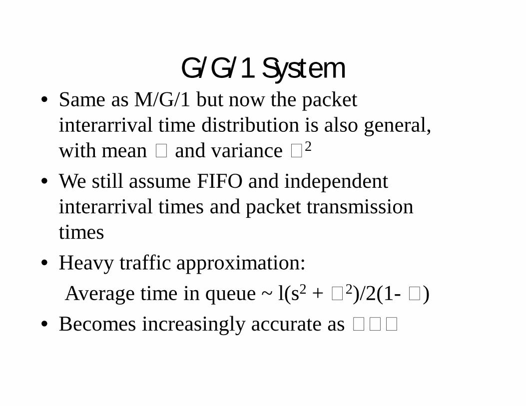
G/G/1 System• Same as M/G/1 but now the packet
interarrival time distribution is also general, with mean and variance 2
• We still assume FIFO and independent interarrival times and packet transmission times
• Heavy traffic approximation:Average time in queue ~ l(s2 + 2)/2(1- )
• Becomes increasingly accurate as
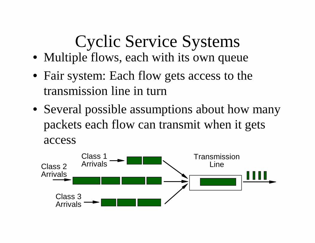
Cyclic Service Systems• Multiple flows, each with its own queue• Fair system: Each flow gets access to the
transmission line in turn• Several possible assumptions about how many
packets each flow can transmit when it gets access
Class 1 Arrivals
Transmission Line
Class 3 Arrivals
Class 2 Arrivals
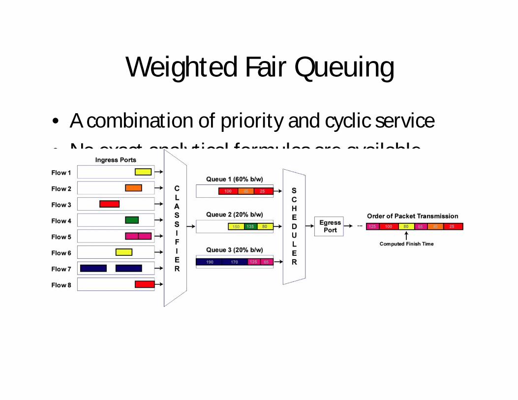
Weighted Fair Queuing
• A combination of priority and cyclic service• No exact analytical formulas are available
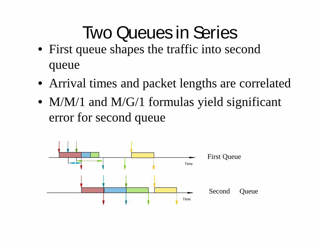
Two Queues in Series• First queue shapes the traffic into second
queue• Arrival times and packet lengths are correlated• M/M/1 and M/G/1 formulas yield significant
error for second queue
Time
First Queue
Time
Second Queue
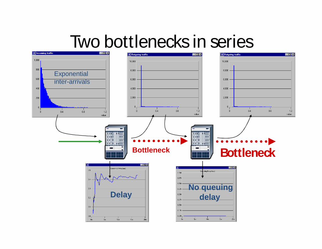
Two bottlenecks in series
Bottleneck
Exponentialinter-arrivals
Bottleneck
No queuing delayDelay
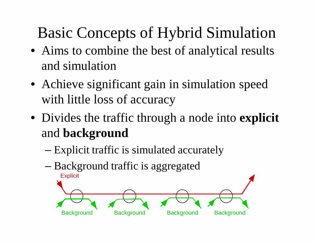
Basic Concepts of Hybrid Simulation• Aims to combine the best of analytical results
and simulation• Achieve significant gain in simulation speed
with little loss of accuracy• Divides the traffic through a node into explicit
and background– Explicit traffic is simulated accurately– Background traffic is aggregated
Explicit
Background BackgroundBackgroundBackground
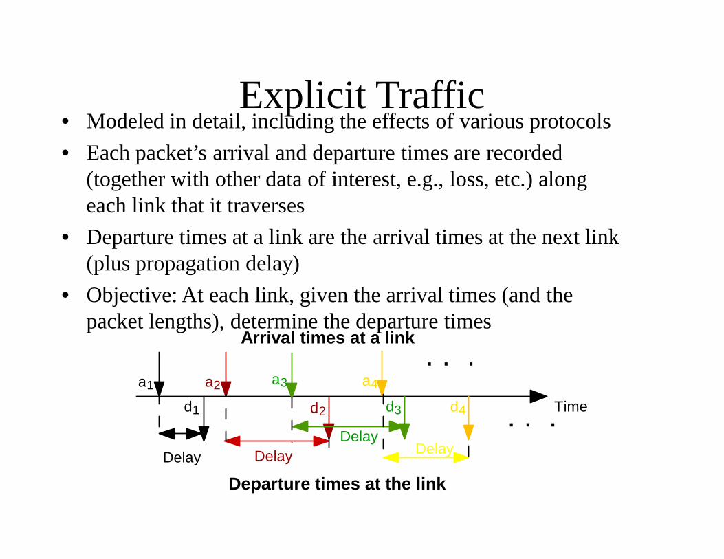
Explicit Traffic• Modeled in detail, including the effects of various protocols• Each packet’s arrival and departure times are recorded
(together with other data of interest, e.g., loss, etc.) along each link that it traverses
• Departure times at a link are the arrival times at the next link (plus propagation delay)
• Objective: At each link, given the arrival times (and the packet lengths), determine the departure times
Time
a1 a2 a3 a4
d1 d4d2 d3
. . .
. . .Delay Delay
DelayDelay
Arrival times at a link
Departure times at the link
Aggregated Traffic• Simplified modeling
– We don’t keep track of individual packets, only workload counts (number of packets or bytes)
– We “generate” workload counts• by probabilistic/analytical modeling, or• by simplified simulation
• Aggregated (or background) traffic is local (per link)• Shaping effects are complex to incorporate• Some dependences between explicit and background
traffic along a chain of links are complicated and are ignored
Steady-State Queue Length Distribution
• If the interval between two successive explicit packets is very long, we can assume that the queue found by the second packet is in steady state.So, we can obtain wk+1 by sampling the steady-state distribution
• Applies to cases where the steady-state distribution can be found or can be reasonably approximated– M/M/1 and other M/M/. Queues– Some M/G/. systems
Self-Similarity in Network Traffic

What is Self-Similarity?
• Self-similarity describes the phenomenon where a certain property of an object is preserved with respect to scaling in space and/or time.
• If an object is self-similar, its parts, when magnified, resemble the shape of the whole.
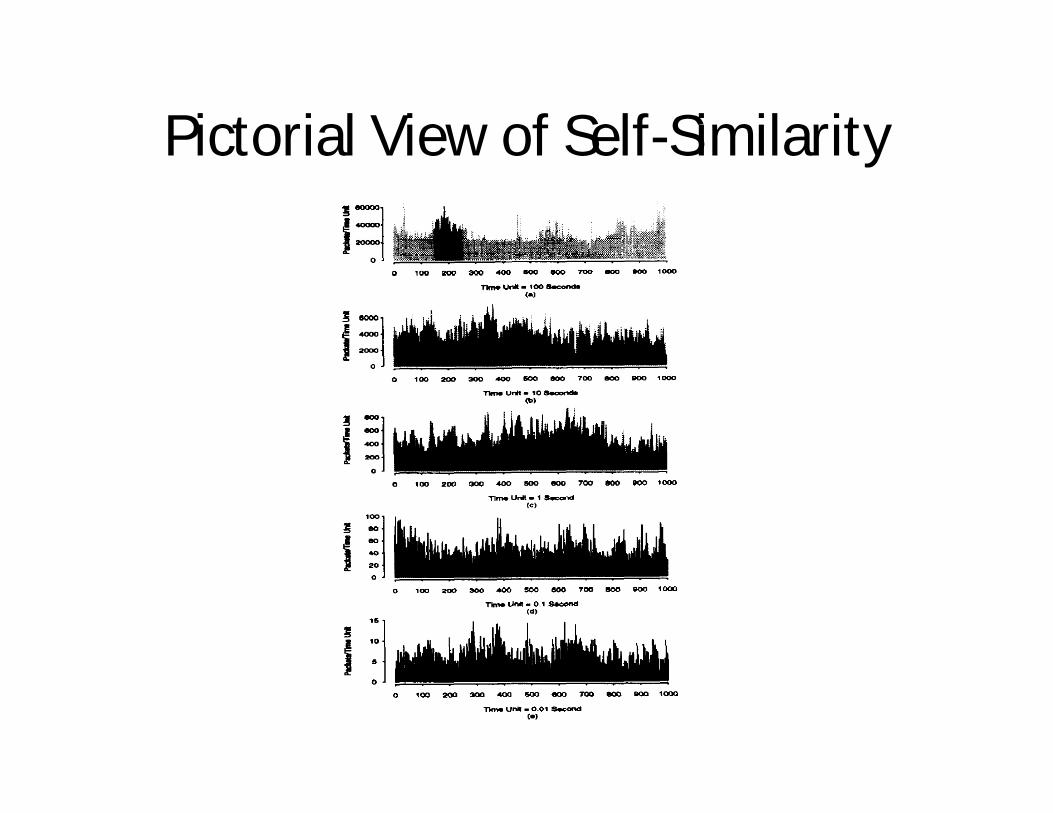
Pictorial View of Self-Similarity
Why is Self-Similarity Important?
• Recently, network packet traffic has been identified as being self-similar.
• Current network traffic modeling using Poisson distributing (etc.) does not take into account the self-similar nature of traffic.
• This leads to inaccurate modeling which, when applied to a huge network like the Internet, can lead to huge financial losses.
Definitions and Properties
• Long-range Dependence– covariance decays slowly
• Hurst Parameter– Developed by Harold Hurst (1965)– H is a measure of “burstiness”
• also considered a measure of self-similarity– 0 < H < 1– H increases as traffic increases
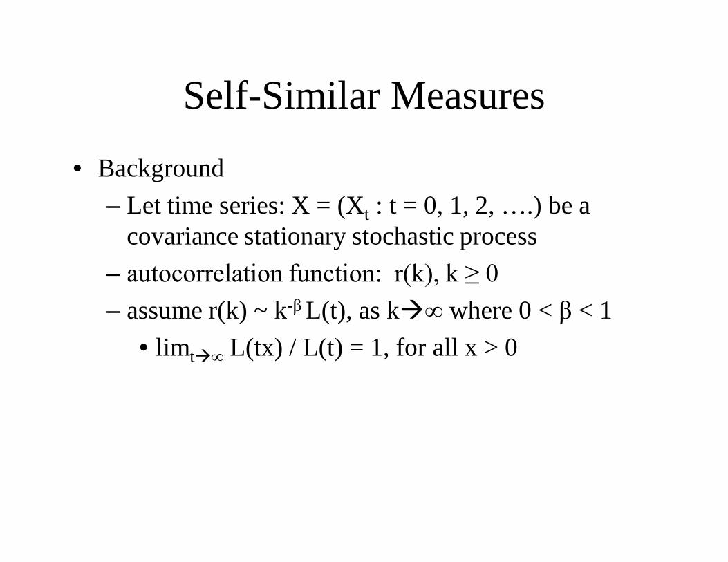
Self-Similar Measures
• Background– Let time series: X = (Xt : t = 0, 1, 2, ….) be a
covariance stationary stochastic process– autocorrelation function: r(k), k ≥ 0– assume r(k) ~ k-β L(t), as k∞ where 0 < β < 1
• limt∞ L(tx) / L(t) = 1, for all x > 0
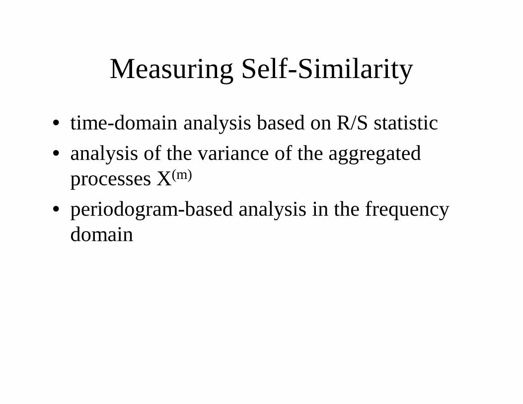
Measuring Self-Similarity
• time-domain analysis based on R/S statistic• analysis of the variance of the aggregated
processes X(m)
• periodogram-based analysis in the frequency domain


![Cis TelePresenCo Ce isDn link...ISDN PRI Interface 1 testShutdown ISDN BRI Interface [1..4] testLoopmode ISDN BRI Interface [1..4] testPattern Cisco telePresence ISDN Link Administrator](https://img.pdfslide.net/doc/110x75/6131c5191ecc51586944f1c2/cis-telepresenco-ce-isdn-link-isdn-pri-interface-1-testshutdown-isdn-bri-interface.jpg)