UNIT III

INTERFERENCE

Cochannel Interference: The frequency-re method is useful for increasing the efficiency of

spectrum usage but results in cochannel interference because the same frequency channel is used

repeatedly in different cochannel cells. Application of the cochannel interference reduction factor

q= D/R = 4.6 for a seven- cell reuse pattern (K = 7). In most mobile radio environments, use of a

seven-cell reuse pattern is not sufficient to avoid cochannel interference. Increasing K > 7 would

reduce the number of channels per cell, and that would also reduce spectrum efficiency.

Therefore, it might be advisable to retain the same number of radios as the seven-cell system but

to sector the cell radially, as if slicing a pie. This technique would reduce cochannel interference

and use channel sharing and channel borrowing schemes to increase spectrum efficiency.

When customer demand increases, the channels which are limited in number, have to be

repeatedly reused in different areas, which provides many cochannel cells, which increases the

system’s capacity. But co channel interference may be the result, in this situation the received

voice quality is affected by both the grade of coverage and the amount of cochannel interference.

For detection of serious channel interference areas in a cellular system, two tests are suggested.

Test 1—find the cochannel interference area from a mobile receiver:

Cochannel interference which occurs in one channel will occur equally in all the other channels in

a given area. We can then measure cochannel interference by selecting any one channel (as one

channel represents all the channels) and transmitting on that channel at all cochannel sites at night

while the mobile receiver is traveling in one of the cochannel cells. While performing this test we

watch for any change detected by a field-strength recorder in the mobile unit and compare the data

with the condition of no cochannel sites being transmitted. This test must be repeated as the

mobile unit travels in every cochannel cell. To facilitate this test, we can install a channel

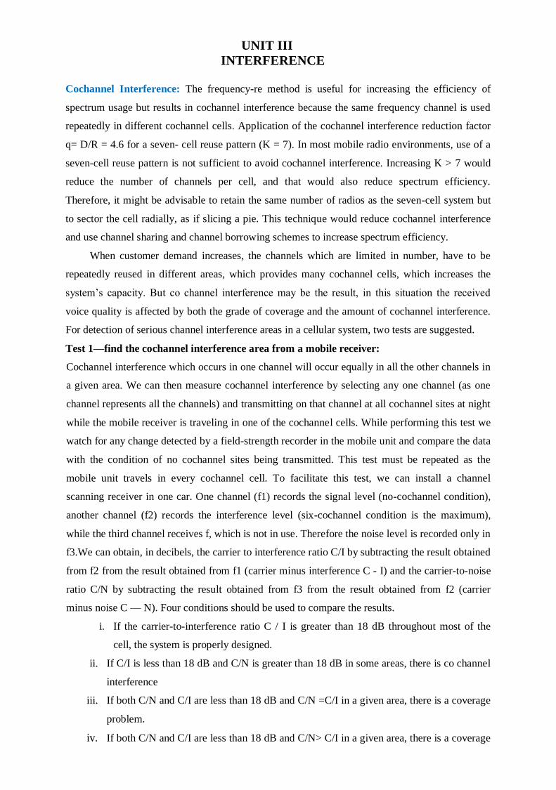
scanning receiver in one car. One channel (f1) records the signal level (no-cochannel condition),

another channel (f2) records the interference level (six-cochannel condition is the maximum),

while the third channel receives f, which is not in use. Therefore the noise level is recorded only in

f3.We can obtain, in decibels, the carrier to interference ratio C/I by subtracting the result obtained

from f2 from the result obtained from f1 (carrier minus interference C - I) and the carrier-to-noise

ratio C/N by subtracting the result obtained from f3 from the result obtained from f2 (carrier

minus noise C — N). Four conditions should be used to compare the results.

i. If the carrier-to-interference ratio C / I is greater than 18 dB throughout most of the

cell, the system is properly designed.

ii. If C/I is less than 18 dB and C/N is greater than 18 dB in some areas, there is co channel

interference

iii. If both C/N and C/I are less than 18 dB and C/N =C/I in a given area, there is a coverage

problem.

iv. If both C/N and C/I are less than 18 dB and C/N> C/I in a given area, there is a coverage

problem and cochannel interference.

Fig.3.1 cochannel interference at mobile unit

Test 2—find the cochannel interference area which affects a cell site:

The reciprocity theorem can be applied for the coverage problem but not for cochannel

interference. Therefore, we cannot assume that the first test result will apply to the second test

condition. We must perform the second test as well. Because it is difficult to use seven cars

simultaneously, with each car traveling in each cochannel cell for this test, an alternative app

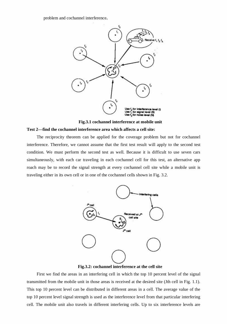
roach may be to record the signal strength at every cochannel cell site while a mobile unit is

traveling either in its own cell or in one of the cochannel cells shown in Fig. 3.2.

Fig.3.2: cochannel interference at the cell site

First we find the areas in an interfering cell in which the top 10 percent level of the signal

transmitted from the mobile unit in those areas is received at the desired site (Jth cell in Fig. 1.1).

This top 10 percent level can be distributed in different areas in a cell. The average value of the

top 10 percent level signal strength is used as the interference level from that particular interfering

cell. The mobile unit also travels in different interfering cells. Up to six interference levels are

obtained from a mobile unit running in six interfering cells. We then calculate the average of the

bottom 10 percent level of the signal strength which is transmitted from a mobile unit in the

desired cell (Jth cell) and received at the desired cell site as a carrier reception level. Then we can

reestablish the carrier-to-interference ratio received at a desired cell, say, the Jth cell site as

follows.The number of cochannel cells in the system can be less than six. We must be aware that

all Cj and Ii were read in decibels, Therefore, a translation from decibels to linear is needed before

summing all the interfering sources. The test can be carried out repeatedly for any given cell. We

then compare Cj/I and Cj/N and determine the cochannel interference condition, which will be the

same as that in test 1. Nj is the noise level in the Jth cell assuming no interference exists.

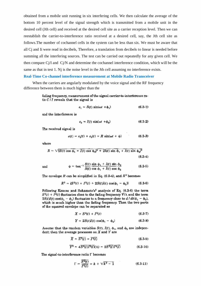
Real-Time Co-channel interference measurement at Mobile Radio Transceiver

When the carriers are angularly modulated by the voice signal and the RF frequency

difference between them is much higher than the

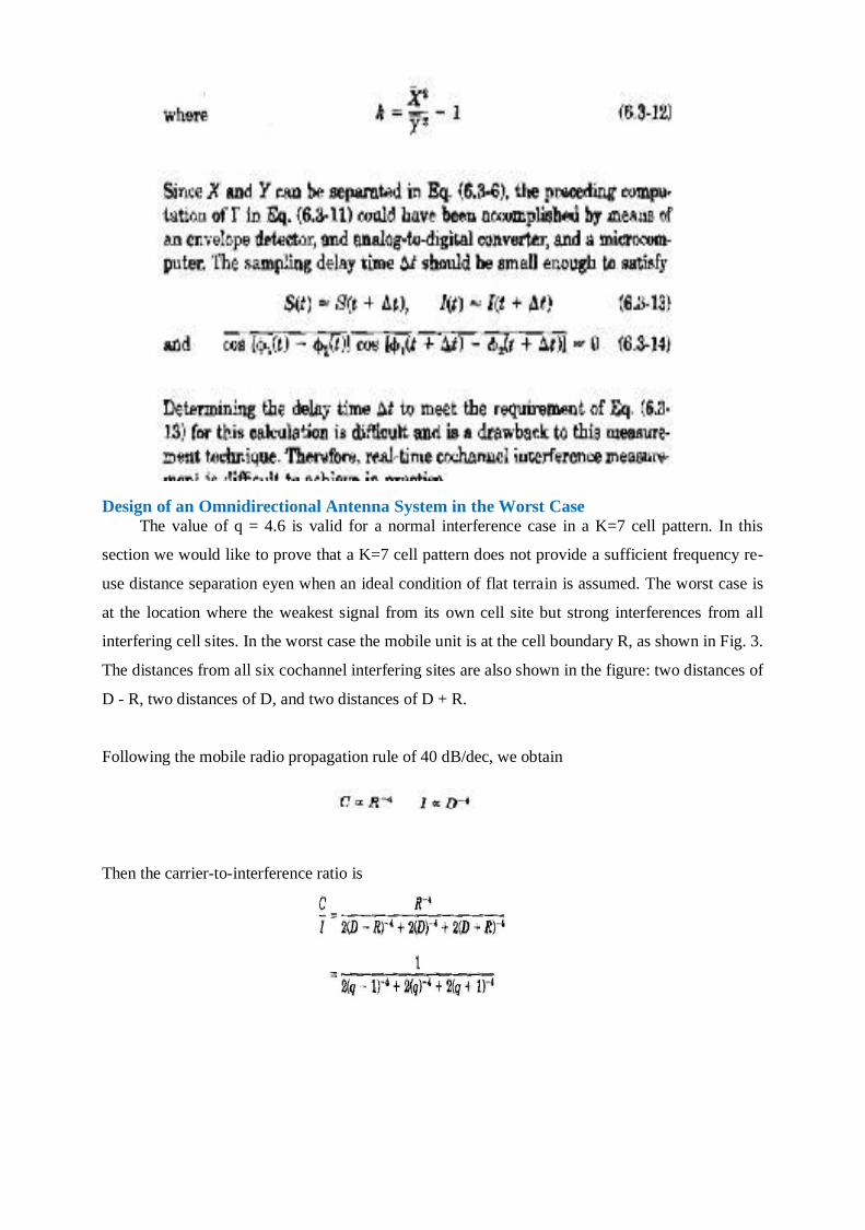
Design of an Omnidirectional Antenna System in the Worst Case The value of q = 4.6 is valid for a normal interference case in a K=7 cell pattern. In this

section we would like to prove that a K=7 cell pattern does not provide a sufficient frequency re-

use distance separation eyen when an ideal condition of flat terrain is assumed. The worst case is

at the location where the weakest signal from its own cell site but strong interferences from all

interfering cell sites. In the worst case the mobile unit is at the cell boundary R, as shown in Fig. 3.

The distances from all six cochannel interfering sites are also shown in the figure: two distances of

D - R, two distances of D, and two distances of D + R.

Following the mobile radio propagation rule of 40 dB/dec, we obtain

Then the carrier-to-interference ratio is

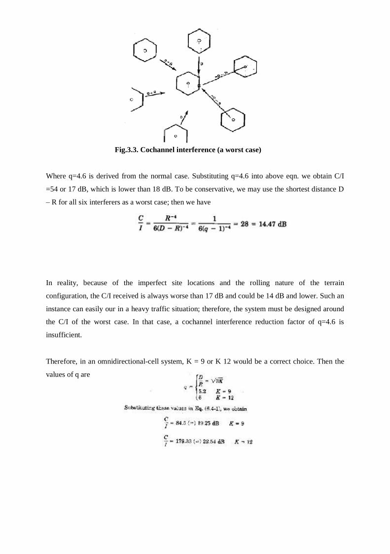
Fig.3.3. Cochannel interference (a worst case)

Where q=4.6 is derived from the normal case. Substituting q=4.6 into above eqn. we obtain C/I

=54 or 17 dB, which is lower than 18 dB. To be conservative, we may use the shortest distance D

– R for all six interferers as a worst case; then we have

In reality, because of the imperfect site locations and the rolling nature of the terrain

configuration, the C/I received is always worse than 17 dB and could be 14 dB and lower. Such an

instance can easily our in a heavy traffic situation; therefore, the system must be designed around

the C/I of the worst case. In that case, a cochannel interference reduction factor of q=4.6 is

insufficient.

Therefore, in an omnidirectional-cell system, K = 9 or K 12 would be a correct choice. Then the

values of q are

Design of a Directional Antenna System:

When the call traffic begins to increase, we need to use the frequency spectrum efficiently

and avoid increasing the number of cells K in a seven-cell frequency reuse pattern. When K

increases, the number of frequency channels assigned in a cell must become smaller (assuming a

total allocated channel divided by K) and the efficiency of applying the frequency reuse scheme

decrease.

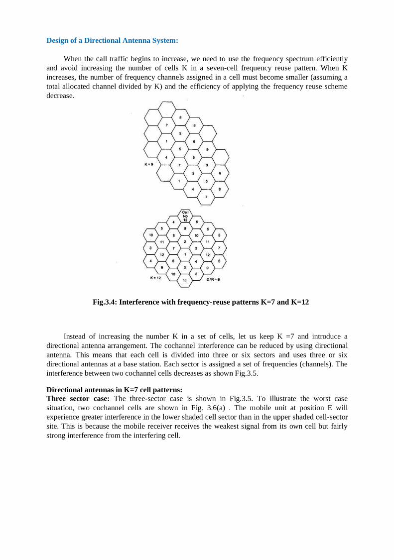
Fig.3.4: Interference with frequency-reuse patterns K=7 and K=12

Instead of increasing the number K in a set of cells, let us keep K =7 and introduce a

directional antenna arrangement. The cochannel interference can be reduced by using directional

antenna. This means that each cell is divided into three or six sectors and uses three or six

directional antennas at a base station. Each sector is assigned a set of frequencies (channels). The

interference between two cochannel cells decreases as shown Fig.3.5.

Directional antennas in K=7 cell patterns: Three sector case: The three-sector case is shown in Fig.3.5. To illustrate the worst case

situation, two cochannel cells are shown in Fig. 3.6(a) . The mobile unit at position E will

experience greater interference in the lower shaded cell sector than in the upper shaded cell-sector

site. This is because the mobile receiver receives the weakest signal from its own cell but fairly

strong interference from the interfering cell.

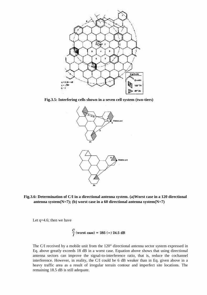
Fig.3.5: Interfering cells shown in a seven cell system (two-tiers)

Fig.3.6: Determination of C/I in a directional antenna system. (a)Worst case in a 120 directional

antenna system(N=7); (b) worst case in a 60 directional antenna system(N=7)

Let q=4.6; then we have

The C/I received by a mobile unit from the 120° directional antenna sector system expressed in

Eq. above greatly exceeds 18 dB in a worst case. Equation above shows that using directional

antenna sectors can improve the signal-to-interference ratio, that is, reduce the cochannel

interference. However, in reality, the C/I could be 6 dB weaker than in Eq. given above in a

heavy traffic area as a result of irregular terrain contour and imperfect site locations. The

remaining 18.5 dB is still adequate.

Six-sector case: We may also divide a cell into six sectors by using six 60°-beam directional

antennas as shown in Fig.4.2. In this case, only one instance of interference can occur in each

sector as shown in Fig, 4.2. Therefore, the carrier-to -interference ratio in this case is which

shows a further reduction of cochannel interference. If we use the same argument as we did for

Eq. above and subtract 6 dB from the result of Eq. the remaining 23 dB is still more than

adequate. When heavy traffic occurs, the 60°-sector configuration can be used to reduce

cochannel interference. However, fewer channels are generally allowed in a 60° sector and the

trunking efficiency decreases. In certain cases, more available channels could be assigned in a

60° sector.

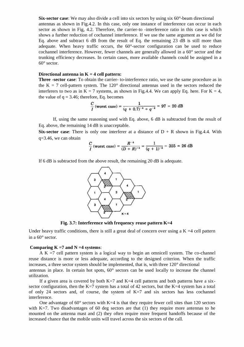
Directional antenna in K = 4 cell pattern: Three -sector case: To obtain the carrier- to-interference ratio, we use the same procedure as in

the K = 7 cell-pattern system. The 120° directional antennas used in the sectors reduced the

interferers to two as in K = 7 systems, as shown in Fig.4.4. We can apply Eq. here. For K = 4,

the value of q = 3.46; therefore, Eq. becomes

If, using the same reasoning used with Eq. above, 6 dB is subtracted from the result of

Eq. above, the remaining 14 dB is unacceptable.

Six-sector case: There is only one interferer at a distance of D + R shown in Fig.4.4. With

q=3.46, we can obtain

If 6 dB is subtracted from the above result, the remaining 20 dB is adequate.

Fig. 3.7: Interference with frequency reuse pattern K=4

Under heavy traffic conditions, there is still a great deal of concern over using a K =4 cell pattern

in a 60° sector.

Comparing K =7 and N =4 systems: A K =7 cell pattern system is a logical way to begin an omnicell system. The co-channel

reuse distance is more or less adequate, according to the designed criterion. When the traffic

increases, a three sector system should be implemented, that is, with three 120° directional

antennas in place. In certain hot spots, 60° sectors can be used locally to increase the channel

utilization.

If a given area is covered by both K=7 and K=4 cell patterns and both patterns have a six-

sector configuration, then the K=7 system has a total of 42 sectors, but the K=4 system has a total

of only 24 sectors and, of course, the system of K=7 and six sectors has less cochannel

interference. One advantage of 60° sectors with K=4 is that they require fewer cell sites than 120 sectors

with K=7. Two disadvantages of 60 deg sectors are that (1) they require more antennas to he

mounted on the antenna mast and (2) they often require more frequent handoffs because of the

increased chance that the mobile units will travel across the six sectors of the call.

Furthermore, assigning the proper frequency channel to the mobile unit in each sector is

more difficult unless the antenna height at the cell site is increased so that the mobile unit can be

located more precisely. In reality the terrain is not flat, end coverage is never uniformly

distributed; in addition, the directional antenna front-to-back power ratio in the field is very

difficult to predict. In small cells, interference could become uncontrollable; then the use of a K =

4 pattern with 60 deg sectors in small cells needs to be considered only for special

implementations such an portable cellular systems or narrow beam applications. For small cells, a

better alternative scheme is to use a K =7 pattern with 120° sectors plus the underlay-overlay

configuration.

Lowering the Antenna Height:

Lowering the antenna height does not always reduce the co-channel interference. In some

circumstances, such as on fairly flat ground or in a valley situation, lowering the antenna height

will be very effective for reducing the cochannel and adjacent-channel interference, However,

there are three cases where lowering the antenna height may or may not effectively help reduce

the interference.

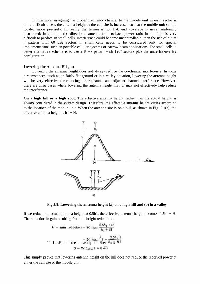
On a high hill or a high spot: The effective antenna height, rather than the actual height, is

always considered in the system design. Therefore, the effective antenna height varies according

to the location of the mobile unit. When the antenna site is on a bill, as shown in Fig. 5.1(a), the

effective antenna height is h1 + H.

Fig 3.8: Lowering the antenna height (a) on a high hill and (b) in a valley

If we reduce the actual antenna height to 0.5h1, the effective antenna height becomes 0.5h1 + H.

The reduction in gain resulting from the height reduction is

If h1<<H, then the above equation becomes

This simply proves that lowering antenna height on the kill does not reduce the received power at

either the cell site or the mobile unit.

In a valley: The effective antenna height as seen from the mobile unit shown in Fig. 5.1(b) is he1,

which is less than the actual antenna height h1. If he1= 2/3 h1, and the antenna is lowered to ½ h1,

then the new effective antenna height is

Then the antenna gain is reduced by

This simply proves that the lowered antenna height in a valley is very effective in reducing the

radiated power in a distant high elevation area. However, in the area adjacent to the cell-site

antenna the effective antenna height is the same as the actual antenna height. The power reduction

caused by decreasing antenna height by half is only

In a forested area: In a forested area, the antenna should clear the tops of any trees in the

vicinity, especially when they are very close to the antenna. In this case decreasing the height of

the antenna would not be the proper procedure for reducing cochannel interference because

excessive attenuation of the desired signal would occur in the vicinity of the antenna and in its cell

boundary if the antenna were below the treetop level.

Antenna Parameters and their effects

The different methods used to reduce co-channel interference are broadly classified into

three. They are

1. By providing large separation among the two co-channel cells.

2. By reducing the antenna heights at the base station.

3. By the usage of directional antennas at the base station.

The first two techniques ne not employed because they have disadvantageous effects i.e.,

method 1 is responsible for reducing the system efficiency for increase in number for

frequency range channels. While method 2 is responsible for reducing the reception level at

the mobile unit. The method 3 is most commonly used because, along with reducing co-

channel interference, it also increases the channel capacity (during heavy traffic).

There are different techniques to generate directional antennas

Tilting the antenna and creating a notch along the unwanted space.

Using umbrella patterns.

Using parasitic elements.

1. Tilting the Antenna: The tilting of an antenna in a desired manner produces an energy

pattern with a notch in the desired direction. Hence, ibis notch prevents the co-channel

interference problem. The tilting of the antenna is done in two ways.

(1) Electrically (ii) Mechanically

In the electronic down tilting, the phases between the elements of a co-linear array antenna are

varied. In the mechanical down tilting the physical rotation of antenna is occurred.

2. Umbrella Pattern: The umbrella pattern is obtained with the help of a staggered discone

antenna. The umbrella pattern reduces the long distance co-channel interference problems,

particularly cross talk. Even though, the umbrella pattern is not used for a directional antenna

pattern, it can be used for an omnidirectional antenna pattern. In hilly areas, where the height of

antenna cannot be increased to cover weak signal spots, results in co-channel interference. In this

case also we can use umbrella pattern. The umbrella pattern allows us to increase the antenna

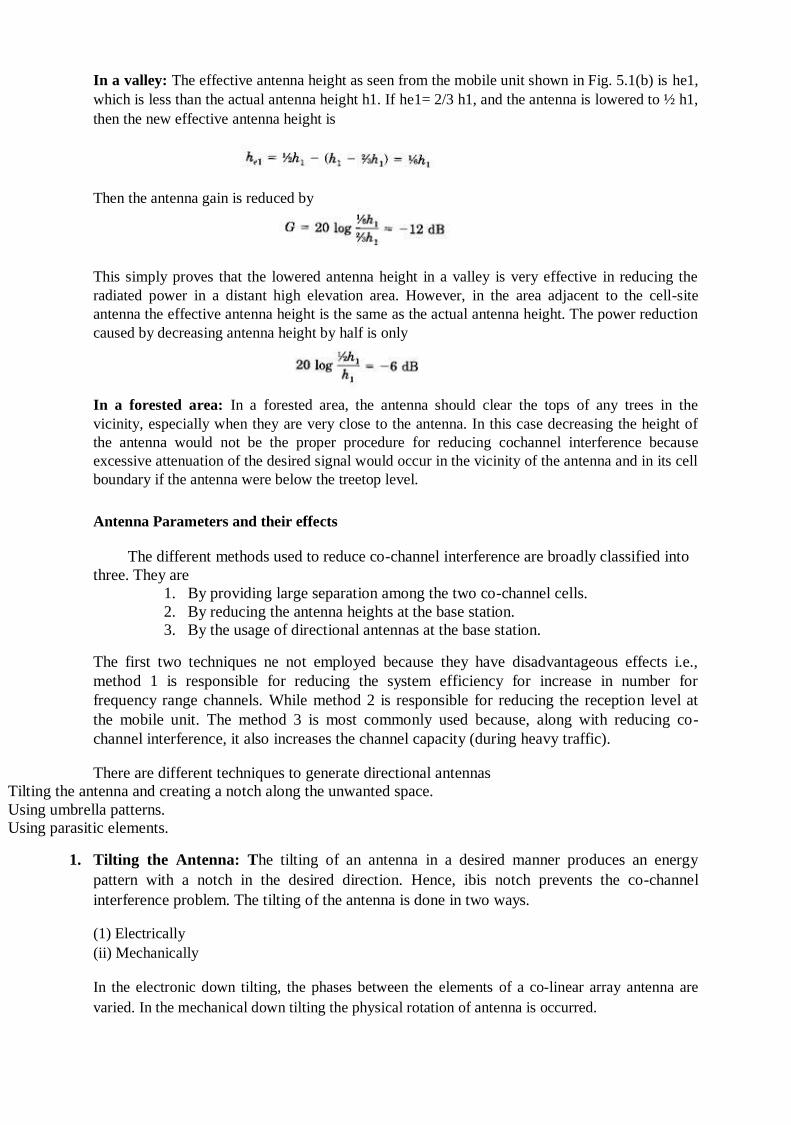
height but, we can still decrease cochannel interference. 3. Parasitic Elements: The use of parasitic elements provides the desired pattern and hence we

can avoid the cochannel interference. This antenna combination has a parasitic antenna and a

driving antenna, the driving antenna is the source of current flowing in the parasitic antenna. The

different combinations of their arrangements produce different patterns as described below.

When the lengths of the elements are identical and closely spaced the current flowing through

the parasitic clement is strong. This creates equal level of patterns.

When the length of parasite is more than drive antenna, the parasite act as reflector and the pattern

in the reflected direction is more.

When the length of parasite is less than drive antenna, the parasite acts as a director and the

pattern is more inclined in the forward direction. These three patterns are illustrated in figure (a)

figure (b) and figure (c) respectively.

Fig 3.9: Antenna patterns with different parasite lengths

Channel Combiner:

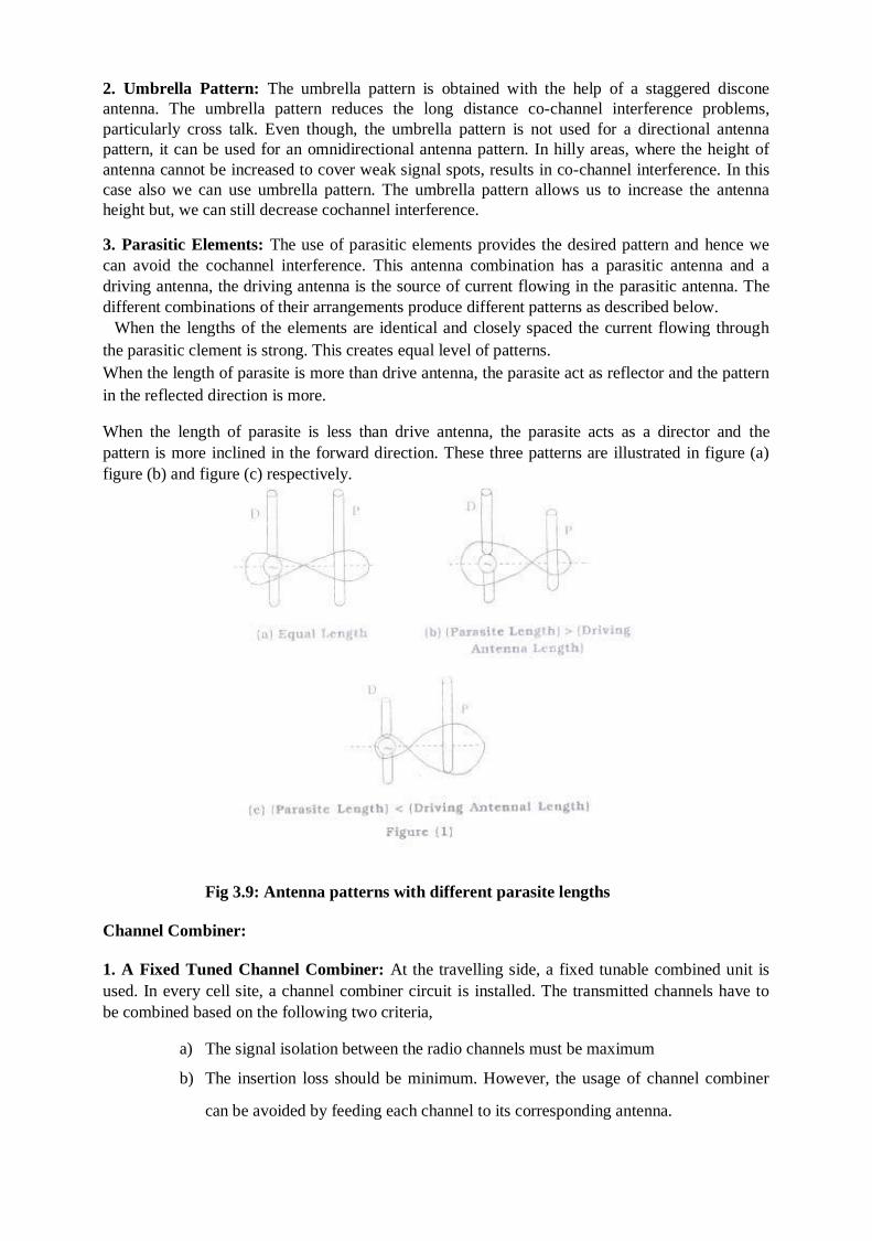
1. A Fixed Tuned Channel Combiner: At the travelling side, a fixed tunable combined unit is

used. In every cell site, a channel combiner circuit is installed. The transmitted channels have to

be combined based on the following two criteria,

a) The signal isolation between the radio channels must be maximum

b) The insertion loss should be minimum. However, the usage of channel combiner

can be avoided by feeding each channel to its corresponding antenna.

But, if there are I6 channels available in a cell site, there will be requirement of 16 antennas

for operation which is bottle neck for real time functionalities. It is not economical to hive huge

hardware setups. Thus, a conventional combiner can he used, which has 16 channel combining

capacity and it is based on the frequency subset of 16 channels of cell site.

The channel combiner would be responsible for each of the 16 channels to exhibit a 3 dB

loss due to the signal insertion in to the channel combiner. The signal isolation would be 17dB, if

every channel is separated from its neighboring channels by 630 kHz frequency.

2. Tunable Combiner: Tunable combiner is also referred as frequency agile combiner. The

frequency agile combiner is an advanced combiner circuit with additional features. It can return

any frequency in real time by remote control device, namely microprocessor. This combiner is

essentially a waveguide resonator with a tuning bar facility. A motor makes the tuning bar to

rotate and once the motor starts rotating, the Voltage Standing Wave Ratio (VSWR) can be

measured.

The controller unit has self-adjusting feature and it accepts an optimum value of VSWR as the

motor complete, a full turn. The controller is compatible only with dynamic frequency assignment.

The cell-sites should be flexible to change their operating frequency ‘f’ that is controlled by

MTSO/MSC. Thus, we can use this frequency agile combiner in the cell site transceiver setup.

3. Ring Combiner: Ring combiner is used to combine two groups of channels to give one output.

This combiner has an insertion loss of 3 dB. For example, using a ring combiner two 16 channel

groups into one 32 channel output. Even 64 channels can be used with this combiner if two

antennas arc available in the cell site. In case of low transmitter power more than one ring

combiner can be used for combining. However, the demerits of ring combiners are.

a) It reduces adjacent-channel separation.

b) They may be affected from the problem of power limitations

Fig 3.10: Channel Combiners

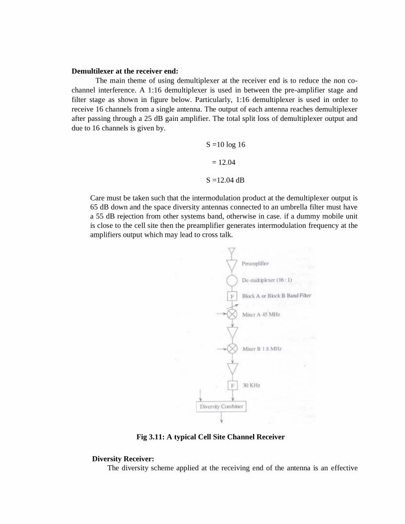
Demultilexer at the receiver end:

The main theme of using demultiplexer at the receiver end is to reduce the non co-

channel interference. A 1:16 demultiplexer is used in between the pre-amplifier stage and

filter stage as shown in figure below. Particularly, 1:16 demultiplexer is used in order to

receive 16 channels from a single antenna. The output of each antenna reaches demultiplexer

after passing through a 25 dB gain amplifier. The total split loss of demultiplexer output and

due to 16 channels is given by.

S =10 log 16

= 12.04

S =12.04 dB

Care must be taken such that the intermodulation product at the demultiplexer output is

65 dB down and the space diversity antennas connected to an umbrella filter must have

a 55 dB rejection from other systems band, otherwise in case. if a dummy mobile unit

is close to the cell site then the preamplifier generates intermodulation frequency at the

amplifiers output which may lead to cross talk.

Fig 3.11: A typical Cell Site Channel Receiver

Diversity Receiver:

The diversity scheme applied at the receiving end of the antenna is an effective

technique for reducing interference because any measures taken at the receiving end to

improve signal performance will not cause additional interference. The diversity

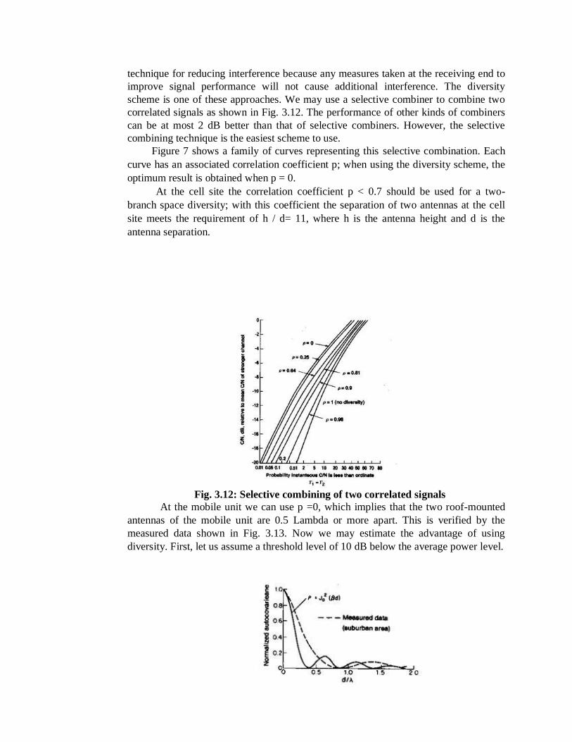
scheme is one of these approaches. We may use a selective combiner to combine two

correlated signals as shown in Fig. 3.12. The performance of other kinds of combiners

can be at most 2 dB better than that of selective combiners. However, the selective

combining technique is the easiest scheme to use.

Figure 7 shows a family of curves representing this selective combination. Each

curve has an associated correlation coefficient p; when using the diversity scheme, the

optimum result is obtained when p = 0.

At the cell site the correlation coefficient p < 0.7 should be used for a two-

branch space diversity; with this coefficient the separation of two antennas at the cell

site meets the requirement of h / d= 11, where h is the antenna height and d is the

antenna separation.

Fig. 3.12: Selective combining of two correlated signals

At the mobile unit we can use p =0, which implies that the two roof-mounted

antennas of the mobile unit are 0.5 Lambda or more apart. This is verified by the

measured data shown in Fig. 3.13. Now we may estimate the advantage of using

diversity. First, let us assume a threshold level of 10 dB below the average power level.

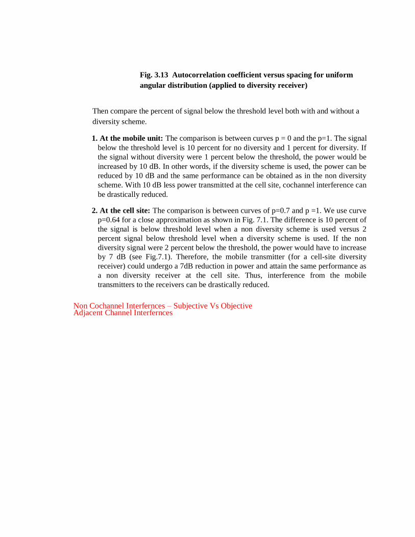
Fig. 3.13 Autocorrelation coefficient versus spacing for uniform

angular distribution (applied to diversity receiver)

Then compare the percent of signal below the threshold level both with and without a

diversity scheme.

1. At the mobile unit: The comparison is between curves p = 0 and the p=1. The signal

below the threshold level is 10 percent for no diversity and 1 percent for diversity. If

the signal without diversity were 1 percent below the threshold, the power would be

increased by 10 dB. In other words, if the diversity scheme is used, the power can be

reduced by 10 dB and the same performance can be obtained as in the non diversity

scheme. With 10 dB less power transmitted at the cell site, cochannel interference can

be drastically reduced.

2. At the cell site: The comparison is between curves of p=0.7 and p =1. We use curve

p=0.64 for a close approximation as shown in Fig. 7.1. The difference is 10 percent of

the signal is below threshold level when a non diversity scheme is used versus 2

percent signal below threshold level when a diversity scheme is used. If the non

diversity signal were 2 percent below the threshold, the power would have to increase

by 7 dB (see Fig.7.1). Therefore, the mobile transmitter (for a cell-site diversity

receiver) could undergo a 7dB reduction in power and attain the same performance as

a non diversity receiver at the cell site. Thus, interference from the mobile

transmitters to the receivers can be drastically reduced.

Non Cochannel Interfernces – Subjective Vs Objective Adjacent Channel Interfernces

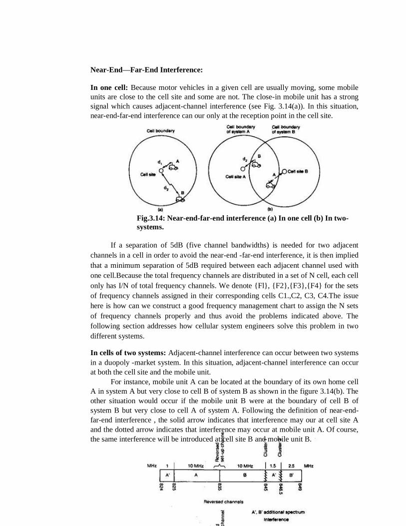
Near-End—Far-End Interference:

In one cell: Because motor vehicles in a given cell are usually moving, some mobile

units are close to the cell site and some are not. The close-in mobile unit has a strong

signal which causes adjacent-channel interference (see Fig. 3.14(a)). In this situation,

near-end-far-end interference can our only at the reception point in the cell site.

Fig.3.14: Near-end-far-end interference (a) In one cell (b) In two-

systems.

If a separation of 5dB (five channel bandwidths) is needed for two adjacent

channels in a cell in order to avoid the near-end -far-end interference, it is then implied

that a minimum separation of 5dB required between each adjacent channel used with

one cell.Because the total frequency channels are distributed in a set of N cell, each cell

only has I/N of total frequency channels. We denote {Fl}, {F2},{F3},{F4} for the sets

of frequency channels assigned in their corresponding cells C1.,C2, C3, C4.The issue

here is how can we construct a good frequency management chart to assign the N sets

of frequency channels properly and thus avoid the problems indicated above. The

following section addresses how cellular system engineers solve this problem in two

different systems.

In cells of two systems: Adjacent-channel interference can occur between two systems

in a duopoly -market system. In this situation, adjacent-channel interference can occur

at both the cell site and the mobile unit.

For instance, mobile unit A can be located at the boundary of its own home cell

A in system A but very close to cell B of system B as shown in the figure 3.14(b). The

other situation would occur if the mobile unit B were at the boundary of cell B of

system B but very close to cell A of system A. Following the definition of near-end-

far-end interference , the solid arrow indicates that interference may our at cell site A

and the dotted arrow indicates that interference may occur at mobile unit A. Of course,

the same interference will be introduced at cell site B and mobile unit B.

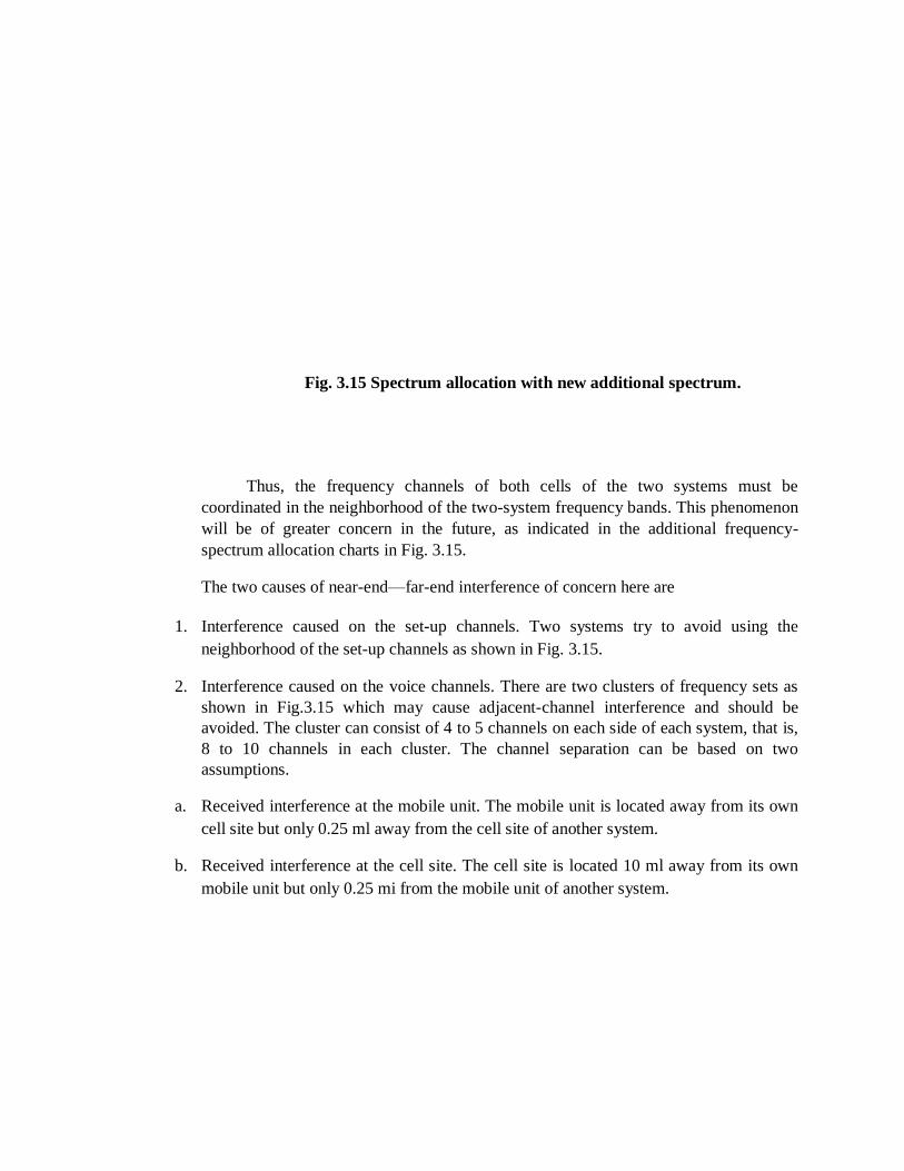
Fig. 3.15 Spectrum allocation with new additional spectrum.

Thus, the frequency channels of both cells of the two systems must be

coordinated in the neighborhood of the two-system frequency bands. This phenomenon

will be of greater concern in the future, as indicated in the additional frequency-

spectrum allocation charts in Fig. 3.15.

The two causes of near-end—far-end interference of concern here are

1. Interference caused on the set-up channels. Two systems try to avoid using the

neighborhood of the set-up channels as shown in Fig. 3.15.

2. Interference caused on the voice channels. There are two clusters of frequency sets as

shown in Fig.3.15 which may cause adjacent-channel interference and should be

avoided. The cluster can consist of 4 to 5 channels on each side of each system, that is,

8 to 10 channels in each cluster. The channel separation can be based on two

assumptions.

a. Received interference at the mobile unit. The mobile unit is located away from its own

cell site but only 0.25 ml away from the cell site of another system.

b. Received interference at the cell site. The cell site is located 10 ml away from its own

mobile unit but only 0.25 mi from the mobile unit of another system.