Embed Size (px)
Citation preview
www.unicourse.org Unit Workbook 3 – Level 4 EEE - U1 Analytical Methods for Engineers – LO3 Calculus author: Michael Lopez BEng(Hons) MSc PGCert CertEd MIFL MIET FHEA ©Unicourse Ltd 2016
Rev3: Feb 2016
Page 1 of 41 1 of 41
online learning
Pearson BTEC Higher Nationals in Electrical and Electronic Engineering (QCF)
Unit 1: Analytical Methods for Engineers (core)
Unit Workbook 3 in a series of 4 for this unit
Learning Outcome
Calculus

www.unicourse.org Unit Workbook 3 – Level 4 EEE - U1 Analytical Methods for Engineers – LO3 Calculus author: Michael Lopez BEng(Hons) MSc PGCert CertEd MIFL MIET FHEA ©Unicourse Ltd 2016
Rev3: Feb 2016
Page 2 of 41 2 of 41
Contents INTRODUCTION .................................................................................................................................................. 3
GUIDANCE .......................................................................................................................................................... 3
3.1 Calculus ................................................................................................................................................... 5
3.1.1 The Concept of the Limit, Continuity and the Derivative ................................................................ 5
3.1.2 Derivatives of Standard Functions ................................................................................................... 6
3.1.3 Notion of the Derivative and Rates of Change .............................................................................. 10
3.1.4 Differentiating a Function of a Function ........................................................................................ 11
3.1.5 The Product Rule ............................................................................................................................ 13
3.1.6 The Quotient Rule .......................................................................................................................... 15
3.1.7 Integral Calculus ............................................................................................................................. 16
3.1.8 Definite Integrals and Areas under Curves .................................................................................... 22
3.2 Further Differentiation .......................................................................................................................... 25
3.2.1 Higher Derivatives .......................................................................................................................... 25
3.2.2 Logarithmic Differentiation ........................................................................................................... 26
3.2.3 Differentiation of Inverse Trigonometric Functions ...................................................................... 29
3.2.4 Differentiation of Inverse Hyperbolic Functions ........................................................................... 30
3.3 Further Integration ................................................................................................................................ 32
3.3.1 Integration by Parts ....................................................................................................................... 32
3.3.2 Integration by Substitution ............................................................................................................ 35
3.3.3 Integration using Partial Fractions ................................................................................................. 36
3.4 Solution of Engineering Problems with Calculus .................................................................................. 39
3.4.1 Charging RC Circuit ........................................................................................................................ 39
3.4.2 Energising Inductor ........................................................................................................................ 40

www.unicourse.org Unit Workbook 3 – Level 4 EEE - U1 Analytical Methods for Engineers – LO3 Calculus author: Michael Lopez BEng(Hons) MSc PGCert CertEd MIFL MIET FHEA ©Unicourse Ltd 2016
Rev3: Feb 2016
Page 3 of 41 3 of 41
Purpose
Theory
Example
INTRODUCTION This Workbook guides you through the learning outcomes related to:
Calculus: the concept of the limit and continuity; definition of the derivative; derivatives of standard
functions; notion of the derivative and rates of change; differentiation of functions using the product,
quotient and function of a function rules; integral calculus as the calculation of area and the inverse of
differentiation; the indefinite integral and the constant of integration; standard integrals and the
application of algebraic and trigonometric functions for their solution; the definite integral and area under
curves
Further differentiation: second order and higher derivatives; logarithmic differentiation; differentiation of
inverse trigonometric functions; differential coefficients of inverse hyperbolic functions
Further integration: integration by parts; integration by substitution; integration using partial fractions
Applications of the calculus: e.g. maxima and minima, points of inflexion, rates of change of temperature,
distance and time, electrical capacitance, rms values, electrical circuit analysis, AC theory, electromagnetic
fields, velocity and acceleration problems, complex stress and strain, engineering structures, simple
harmonic motion, centroids, volumes of solids of revolution, second moments of area, moments of inertia,
rules of Pappus, radius of gyration, thermodynamic work and heat energy
Engineering problems: e.g. stress and strain, torsion, motion, dynamic systems, oscillating systems, force
systems, heat energy and thermodynamic systems, fluid flow, AC theory, electrical signals, information
systems, transmission systems, electrical machines, electronics
GUIDANCE This document is prepared to break the unit material down into bite size chunks. You will see the learning
outcomes above treated in their own sections. Therein you will encounter the following structures;
Explains why you need to study the current section of material. Quite often learners
are put off by material which does not initially seem to be relevant to a topic or
profession. Once you understand the importance of new learning or theory you will
embrace the concepts more readily.
Conveys new material to you in a straightforward fashion. To support the treatments
in this section you are strongly advised to follow the given hyperlinks, which may be
useful documents or applications on the web.
The examples/worked examples are presented in a knowledge-building order. Make
sure you follow them all through. If you are feeling confident then you might like to
treat an example as a question, in which case cover it up and have a go yourself.
Many of the examples given resemble assignment questions which will come your
way, so follow them through diligently.

www.unicourse.org Unit Workbook 3 – Level 4 EEE - U1 Analytical Methods for Engineers – LO3 Calculus author: Michael Lopez BEng(Hons) MSc PGCert CertEd MIFL MIET FHEA ©Unicourse Ltd 2016
Rev3: Feb 2016
Page 4 of 41 4 of 41
Question
Challenge
ee
Video
Questions should not be avoided if you are determined to learn. Please do take the
time to tackle each of the given questions, in the order in which they are presented.
The order is important, as further knowledge and confidence is built upon previous
knowledge and confidence. As an Online Learner it is important that the answers to
questions are immediately available to you. Contact your Unit Tutor if you need help.
You can really cement your new knowledge by undertaking the challenges. A
challenge could be to download software and perform an exercise. An alternative
challenge might involve a practical activity or other form of research.
Videos on the web can be very useful supplements to your distance learning efforts.
Wherever an online video(s) will help you then it will be hyperlinked at the
appropriate point.

www.unicourse.org Unit Workbook 3 – Level 4 EEE - U1 Analytical Methods for Engineers – LO3 Calculus author: Michael Lopez BEng(Hons) MSc PGCert CertEd MIFL MIET FHEA ©Unicourse Ltd 2016
Rev3: Feb 2016
Page 5 of 41 5 of 41
3.1 Calculus There are a couple of great webpages for checking your answers to Calculus problems…
Check Differentiation answers
Check Integration answers
3.1.1 The Concept of the Limit, Continuity and the Derivative Calculus deals with functions which continually vary and is based upon the concept of a limit and
continuity. Let’s refer to a diagram to understand the concept of a limit…
Here we have indicated a point P on part of a function (the red curve) with Cartesian co-ordinates (𝑥1, 𝑦1).
We require another point Q on the function to be a small increment away from P and will designate a small
increment with the symbol 𝛿 (delta).
What we then have is…
𝑷 = (𝒙𝟏, 𝒚𝟏)
𝑸 = (𝒙𝟏 + 𝜹𝒙, 𝒚𝟏 + 𝜹𝒚)
Look now at the chord PQ (drawn as the straight line in blue). If we can determine the slope of this chord
and then make it infinitesimally short we will end up with a tangent to the function. It is the slope of this
tangent which forms the basis of Differential Calculus (normally called differentiation).
By inspection, we see that the slope of the chord is given by…
𝒔𝒍𝒐𝒑𝒆 𝒐𝒇 𝒄𝒉𝒐𝒓𝒅 𝑷𝑸 =𝜹𝒚
𝜹𝒙

www.unicourse.org Unit Workbook 3 – Level 4 EEE - U1 Analytical Methods for Engineers – LO3 Calculus author: Michael Lopez BEng(Hons) MSc PGCert CertEd MIFL MIET FHEA ©Unicourse Ltd 2016
Rev3: Feb 2016
Page 6 of 41 6 of 41
Worked Example 1
If we deliberately make 𝛿𝑥 approach zero (i.e. make it as short as possible) then we shall reach a limit,
which may expressed mathematically as…
𝒅𝒚
𝒅𝒙= 𝜹𝒙
𝒍𝒊𝒎𝒊𝒕→ 𝟎
𝜹𝒚
𝜹𝒙
The term 𝑑𝑦 𝑑𝑥⁄ is written in Leibnitz notation and indicates the slope of the chord when the chord only
touches the function at one single point. This is achieved by continual reduction of 𝛿𝑥.
What we can now say is that we are able to find the slope of any function by adopting this process. Hence,
given a function 𝑓(𝑥) we are able to differentiate that function, meaning find its slope at all points. We can
write…
The slope at any point of a function 𝑓(𝑥) is given by 𝒅(𝒇(𝒙))
𝒅𝒙
This process is called finding the derivative of a function.
3.1.2 Derivatives of Standard Functions What we don’t want to be doing is to spend too much time drawing graphs of functions just to work out
the derivative. Fortunately there are standard ways to determine the derivative of functions and some of
the frequent ones which engineers meet are given in the table below.
Function Derivative 𝐴𝑥𝑛 𝑛𝐴𝑥𝑛−1
A sin (𝑥) A cos (𝑥)
A cos (𝑥) −𝐴 sin (𝑥)
𝐴 𝑒𝑘𝑥 𝑘𝐴𝑒𝑘𝑥
𝐴 𝑙𝑜𝑔𝑒(𝑥) 𝐴𝑥⁄
A sinh (𝑥) A cosh (𝑥)
A cosh (𝑥) A sinh (𝑥)
Let’s look at some examples of using these standard derivatives…

www.unicourse.org Unit Workbook 3 – Level 4 EEE - U1 Analytical Methods for Engineers – LO3 Calculus author: Michael Lopez BEng(Hons) MSc PGCert CertEd MIFL MIET FHEA ©Unicourse Ltd 2016
Rev3: Feb 2016
Page 7 of 41 7 of 41
Worked Example 2
Worked Example 3
Worked Example 4
Differentiate the function 𝒚 = 𝟑𝒙𝟒 with respect to 𝒙.
We see that this function is similar to that in row 1 of our table. We can see that 𝐴 = 3 and 𝑛 = 4. We may
then write…
𝑑𝑦
𝑑𝑥= 𝑛𝐴𝑥𝑛−1 = (4)(3)𝑥4−1 = 12𝑥3
Differentiate the function 𝒚 = 𝟔𝒙−𝟓 with respect to 𝒙.
We see that this function is similar to that in row 1 of our table. We can see that 𝐴 = 6 and 𝑛 = −5. We
may then write…
𝑑𝑦
𝑑𝑥= 𝑛𝐴𝑥𝑛−1 = (−5)(6)𝑥−5−1 = −30𝑥−6
Differentiate the function 𝒗 = 𝟏𝟐 𝒔𝒊𝒏(𝒕) with respect to 𝒕.
Don’t worry that 𝑦 and 𝑥 have disappeared here. We can use any letters we like. The letter 𝑣 means
voltage and 𝑡 is time. All we want to do here then is to find 𝑑𝑣 𝑑𝑡⁄ .
We see that the function is similar to that in row 2 of our table. We may write…
𝑑𝑣
𝑑𝑡= 𝐴 cos(𝑡) = 12 cos (𝑡)
Differentiate the function 𝒊 = 𝟓 𝒄𝒐𝒔(𝒕) with respect to 𝒕.

www.unicourse.org Unit Workbook 3 – Level 4 EEE - U1 Analytical Methods for Engineers – LO3 Calculus author: Michael Lopez BEng(Hons) MSc PGCert CertEd MIFL MIET FHEA ©Unicourse Ltd 2016
Rev3: Feb 2016
Page 8 of 41 8 of 41
Worked Example 5
Worked Example 6
Worked Example 7
Worked Example 8
The letter 𝑖 means current and 𝑡 is time. All we want to do here then is to find 𝑑𝑖 𝑑𝑡⁄ .
We see that the function is similar to that in row 3 of our table. We may write…
𝑑𝑖
𝑑𝑡= −𝐴 sin(𝑡) = −5 sin (𝑡)
Differentiate the function 𝒚 = 𝟒𝒆𝟐𝒙 with respect to 𝒙.
From row 4 of our table we can write…
𝑑𝑦
𝑑𝑥= 𝑘𝐴𝑒𝑘𝑥 = (2)(4)𝑒2𝑥 = 8𝑒2𝑥
Differentiate the function 𝒚 = 𝟏𝟔 𝒍𝒐𝒈𝒆(𝒙) with respect to 𝒙.
We refer to row 5 of our table and write…
𝑑𝑦
𝑑𝑥=𝐴
𝑥=16
𝑥
Differentiate the function 𝒚 = 𝟗 𝒔𝒊𝒏𝒉(𝒙) with respect to 𝒙.
We refer to row 6 of our table and write…
𝑑𝑦
𝑑𝑥= 𝐴 cosh(𝑥) = 9 cosh (𝑥)
Differentiate the function 𝒚 = −𝟏𝟒. 𝟓 𝒄𝒐𝒔𝒉(𝒙) with respect to 𝒙.
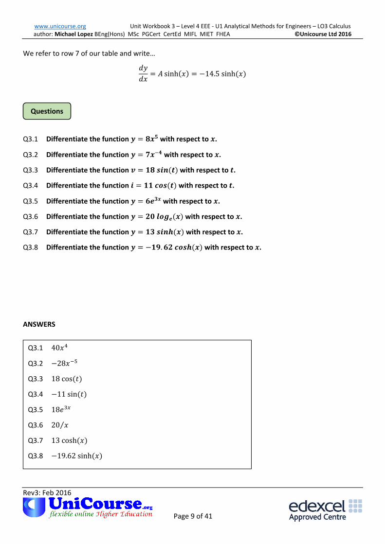
www.unicourse.org Unit Workbook 3 – Level 4 EEE - U1 Analytical Methods for Engineers – LO3 Calculus author: Michael Lopez BEng(Hons) MSc PGCert CertEd MIFL MIET FHEA ©Unicourse Ltd 2016
Rev3: Feb 2016
Page 9 of 41 9 of 41
Questions
We refer to row 7 of our table and write…
𝑑𝑦
𝑑𝑥= 𝐴 sinh(𝑥) = −14.5 sinh (𝑥)
Q3.1 Differentiate the function 𝒚 = 𝟖𝒙𝟓 with respect to 𝒙.
Q3.2 Differentiate the function 𝒚 = 𝟕𝒙−𝟒 with respect to 𝒙.
Q3.3 Differentiate the function 𝒗 = 𝟏𝟖 𝒔𝒊𝒏(𝒕) with respect to 𝒕.
Q3.4 Differentiate the function 𝒊 = 𝟏𝟏 𝒄𝒐𝒔(𝒕) with respect to 𝒕.
Q3.5 Differentiate the function 𝒚 = 𝟔𝒆𝟑𝒙 with respect to 𝒙.
Q3.6 Differentiate the function 𝒚 = 𝟐𝟎 𝒍𝒐𝒈𝒆(𝒙) with respect to 𝒙.
Q3.7 Differentiate the function 𝒚 = 𝟏𝟑 𝒔𝒊𝒏𝒉(𝒙) with respect to 𝒙.
Q3.8 Differentiate the function 𝒚 = −𝟏𝟗. 𝟔𝟐 𝒄𝒐𝒔𝒉(𝒙) with respect to 𝒙.
ANSWERS
Q3.1 40𝑥4
Q3.2 −28𝑥−5
Q3.3 18 cos(𝑡)
Q3.4 −11 sin(𝑡)
Q3.5 18𝑒3𝑥
Q3.6 20 𝑥⁄
Q3.7 13 cosh(𝑥)
Q3.8 −19.62 sinh(𝑥)

www.unicourse.org Unit Workbook 3 – Level 4 EEE - U1 Analytical Methods for Engineers – LO3 Calculus author: Michael Lopez BEng(Hons) MSc PGCert CertEd MIFL MIET FHEA ©Unicourse Ltd 2016
Rev3: Feb 2016
Page 10 of 41 10 of 41
Video These videos will boost your knowledge of differentiation
3.1.3 Notion of the Derivative and Rates of Change The notion of taking the derivative of a function and examining rate of change can be readily explained
with reference to the diagram below…
Here we have plotted a section of a sine wave in red. Notice that we have used pink arrows to indicate the
slope at various points on the sine wave. For example, at the start the sine wave is rising to a positive more
rapidly than at any other point. The pink arrow indicates this positive growth by pointing upwards in the
direction of the sine wave at that beginning point. The second arrow shows the slope of the sine wave at
𝜋 2⁄ radians (or 900 if you like). Here it is at a plateau and has zero slope (meaning that it just moves
horizontally, with no vertical movement at all). The third arrow indicates a negative slope (its moving down
very steeply). The picture continues in a similar way for the remaining arrows.
Here’s the really interesting bit. When we record all of the slopes on our sine wave we get the dotted
waveform in blue. What does that look like? Of course, it is a cosine wave. So we have just proved
graphically that finding the slope (differentiating) at all points on a sine wave leads to a cosine wave.
∴ 𝒅{𝐬𝐢𝐧 (𝒕)}
𝒅𝒕= 𝐜𝐨𝐬 (𝒕)
… as given in our table of standard derivatives in section 3.1.2.
If we had loads of time to kill we could prove all of the other derivatives graphically.

www.unicourse.org Unit Workbook 3 – Level 4 EEE - U1 Analytical Methods for Engineers – LO3 Calculus author: Michael Lopez BEng(Hons) MSc PGCert CertEd MIFL MIET FHEA ©Unicourse Ltd 2016
Rev3: Feb 2016
Page 11 of 41 11 of 41
Challenge
ee
Determine a graphical proof (as above) for…
𝒅{𝐜𝐨𝐬 (𝒕)}
𝒅𝒕= −𝐬𝐢𝐧 (𝒕)
3.1.4 Differentiating a Function of a Function What do we mean by this term ‘function of a function’? Well, the motion of kicking a ball involves moving
your leg, which in turn involves brain activity to control the kick. We can therefore say that kicking a ball is
a ‘function of a function’ of brain activity. So it is with much of mathematics.
If you see a simple function like 𝑦 = 2𝑥 you would agree that is a straight line graph with a slope of 2. It
also a function, because we can plot functions can’t we? What if we looked at something like…
𝒚 = 𝐬𝐢𝐧 (𝟐𝒙)
Is that a function? Yes it is, and we can plot it. But, it is also a function of a function. In fact, it is a sine
function of a 2𝑥 function. How are we then going to evaluate this function of a function? Let’s analyse
what we have…
Let 𝑢 = 2𝑥 ∴ 𝑢 = 2𝑥1 This looks like the first function in our table of standard derivatives. Let’s
differentiate in the way we did in Worked Example 1…
𝒅𝒖
𝒅𝒙= (𝟏)(𝟐)𝒙𝟏−𝟏 = 𝟐𝒙𝟎 = 𝟐 × 𝟏 = 𝟐
OK, so where does that get us? If we now use this 𝑢 in the original question we get…
𝑦 = sin(2𝑥) = sin (𝑢)
Let’s now differentiate that…
𝒅𝒚
𝒅𝒖= 𝐜𝐨𝐬 (𝒖)
The trick in ‘function of a function’ problems is to combine those two derivatives by multiplying them
together…
𝑑𝑢
𝑑𝑥∙𝑑𝑦
𝑑𝑢=𝑑𝑦
𝑑𝑥= 2 cos (𝑢)
Those two 𝑑𝑢 terms have cancelled each other out. Since we know what 𝑢 is (it’s 2𝑥) we can now write the
final answer…
𝒅𝒚
𝒅𝒙= 𝟐 𝐜𝐨𝐬 (𝟐𝒙)

www.unicourse.org Unit Workbook 3 – Level 4 EEE - U1 Analytical Methods for Engineers – LO3 Calculus author: Michael Lopez BEng(Hons) MSc PGCert CertEd MIFL MIET FHEA ©Unicourse Ltd 2016
Rev3: Feb 2016
Page 12 of 41 12 of 41
Worked Example 9
Worked Example 10
Let’s look at a couple of worked examples on the ‘function of a function’ process…
Differentiate 𝒚 = (𝒙𝟒 + 𝟑)𝟐 with respect to 𝒙.
The best approach is to let the term in brackets equal 𝑢 and proceed as before…
𝑳𝒆𝒕 𝒖 = 𝒙𝟒 + 𝟑 ∴ 𝒅𝒖
𝒅𝒙= (𝟒)𝒙𝟒−𝟏 + (𝟎)𝒙𝟎−𝟏 = 𝟒𝒙𝟑
Notice above that the solitary 3 at the end disappeared when we differentiated it. Think about what the
number 3 looks like on a graph. It’s just a horizontal line passing through the 𝑦 axis at the point 𝑦 = 3
right? Sketching it you realise that the slope is zero everywhere on the line. So the golden rule for solitary
numbers is that we ignore them when differentiating. Let’s proceed with the remainder of the original
problem…
𝒚 = (𝒖)𝟐 ∴ 𝒅𝒚
𝒅𝒖= (𝟐)𝒖𝟐−𝟏 = 𝟐𝒖𝟏 = 𝟐𝒖
Combining our results gives…
𝒅𝒚
𝒅𝒙=𝒅𝒖
𝒅𝒙∙𝒅𝒚
𝒅𝒖= 𝟒𝒙𝟑 × 𝟐𝒖 = 𝟒𝒙𝟑 × 𝟐(𝒙𝟒 + 𝟑) = 𝟖𝒙𝟑(𝒙𝟒 + 𝟑) = 𝟖𝒙𝟕 + 𝟐𝟒𝒙𝟑
Differentiate 𝒚 = 𝒄𝒐𝒔(𝟒𝒙𝟑 + 𝟑𝒙−𝟐 − 𝟔𝒙 + 𝟖) with respect to 𝒙.
𝐿𝑒𝑡 𝑢 = 4𝑥3 + 3𝑥−2 − 6𝑥 + 8
∴ 𝒅𝒖
𝒅𝒙= 𝟏𝟐𝒙𝟐 − 𝟔𝒙−𝟑 − 𝟔
𝐴𝑙𝑠𝑜, 𝑦 = cos (𝑢)
www.unicourse.org Unit Workbook 3 – Level 4 EEE - U1 Analytical Methods for Engineers – LO3 Calculus author: Michael Lopez BEng(Hons) MSc PGCert CertEd MIFL MIET FHEA ©Unicourse Ltd 2016
Rev3: Feb 2016
Page 13 of 41 13 of 41
Questions
Video
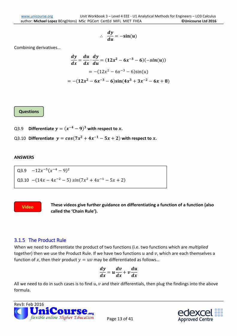
∴ 𝒅𝒚
𝒅𝒖= −𝐬𝐢𝐧 (𝒖)
Combining derivatives…
𝒅𝒚
𝒅𝒙=𝒅𝒖
𝒅𝒙∙𝒅𝒚
𝒅𝒖= (𝟏𝟐𝒙𝟐 − 𝟔𝒙−𝟑 − 𝟔)(−𝒔𝒊𝒏(𝒖))
= −(12𝑥2 − 6𝑥−3 − 6)sin (𝑢)
= −(𝟏𝟐𝒙𝟐 − 𝟔𝒙−𝟑 − 𝟔)𝐬𝐢𝐧 (𝟒𝒙𝟑 + 𝟑𝒙−𝟐 − 𝟔𝒙 + 𝟖)
Q3.9 Differentiate 𝒚 = (𝒙−𝟒 − 𝟗)𝟑 with respect to 𝒙.
Q3.10 Differentiate 𝒚 = 𝒄𝒐𝒔(𝟕𝒙𝟐 + 𝟒𝒙−𝟏 − 𝟓𝒙 + 𝟐) with respect to 𝒙.
ANSWERS
These videos give further guidance on differentiating a function of a function (also
called the ‘Chain Rule’).
3.1.5 The Product Rule When we need to differentiate the product of two functions (i.e. two functions which are multiplied
together) then we use the Product Rule. If we have two functions 𝑢 and 𝑣, which are each themselves a
function of 𝑥, then their product 𝑦 = 𝑢𝑣 may be differentiated as follows…
𝒅𝒚
𝒅𝒙= 𝒖
𝒅𝒗
𝒅𝒙+ 𝒗
𝒅𝒖
𝒅𝒙
All we need to do in such cases is to find 𝑢, 𝑣 and their differentials, then plug the findings into the above
formula.
Q3.9 −12𝑥−5(𝑥−4 − 9)2
Q3.10 −(14𝑥 − 4𝑥−2 − 5) 𝑠𝑖𝑛(7𝑥2 + 4𝑥−1 − 5𝑥 + 2)
www.unicourse.org Unit Workbook 3 – Level 4 EEE - U1 Analytical Methods for Engineers – LO3 Calculus author: Michael Lopez BEng(Hons) MSc PGCert CertEd MIFL MIET FHEA ©Unicourse Ltd 2016
Rev3: Feb 2016
Page 14 of 41 14 of 41
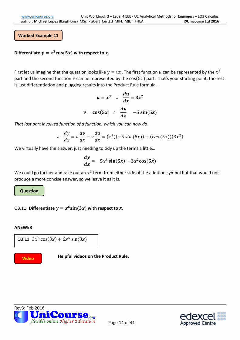
Worked Example 11
Question
Video
Differentiate 𝒚 = 𝒙𝟑𝐜𝐨𝐬 (𝟓𝒙) with respect to 𝒙.
First let us imagine that the question looks like 𝑦 = 𝑢𝑣. The first function 𝑢 can be represented by the 𝑥3
part and the second function 𝑣 can be represented by the cos (5𝑥) part. That’s your starting point, the rest
is just differentiation and plugging results into the Product Rule formula…
𝒖 = 𝒙𝟑 ∴ 𝒅𝒖
𝒅𝒙= 𝟑𝒙𝟐
𝒗 = 𝐜𝐨𝐬(𝟓𝒙) ∴ 𝒅𝒗
𝒅𝒙= −𝟓 𝐬𝐢𝐧 (𝟓𝒙)
That last part involved function of a function, which you can now do.
∴ 𝑑𝑦
𝑑𝑥= 𝑢
𝑑𝑣
𝑑𝑥+ 𝑣
𝑑𝑢
𝑑𝑥= (𝑥3)(−5 𝑠𝑖𝑛 (5𝑥)) + (𝑐𝑜𝑠 (5𝑥))(3𝑥2)
We virtually have the answer, just needing to tidy up the terms a little…
𝒅𝒚
𝒅𝒙= −𝟓𝒙𝟑 𝐬𝐢𝐧(𝟓𝒙) + 𝟑𝒙𝟐𝐜𝐨𝐬 (𝟓𝒙)
We could go further and take out an 𝑥2 term from either side of the addition symbol but that would not
produce a more concise answer, so we leave it as it is.
Q3.11 Differentiate 𝒚 = 𝒙𝟔𝐬𝐢𝐧(𝟑𝒙) with respect to 𝒙.
ANSWER
Helpful videos on the Product Rule.
Q3.11 3𝑥6 cos(3𝑥) + 6𝑥5 sin(3𝑥)

www.unicourse.org Unit Workbook 3 – Level 4 EEE - U1 Analytical Methods for Engineers – LO3 Calculus author: Michael Lopez BEng(Hons) MSc PGCert CertEd MIFL MIET FHEA ©Unicourse Ltd 2016
Rev3: Feb 2016
Page 15 of 41 15 of 41
Worked Example 12
Question
3.1.6 The Quotient Rule When we need to differentiate the quotient of two functions (i.e. two functions which are divided) then we
use the Quotient Rule. If we have two functions 𝑢 and 𝑣, which are each themselves a function of 𝑥, then
their quotient 𝑦 = 𝑢 𝑣⁄ may be differentiated as follows…
𝒅𝒚
𝒅𝒙=𝒗𝒅𝒖𝒅𝒙− 𝒖
𝒅𝒗𝒅𝒙
𝒗𝟐
All we need to do in such cases is to find 𝑢, 𝑣 and their differentials, then plug the findings into the above
formula.
Differentiate the following function with respect to 𝒙…
𝒚 =𝒙𝟐
𝒔𝒊𝒏(𝟐𝒙)
𝐿𝑒𝑡 𝑢 = 𝑥2 ∴ 𝑑𝑢
𝑑𝑥= 2𝑥
𝐿𝑒𝑡 𝑣 = sin(2𝑥) ∴ 𝑑𝑣
𝑑𝑥= 2 cos(2𝑥)
Placing these results in the formula gives…
𝑑𝑦
𝑑𝑥=𝑣𝑑𝑢𝑑𝑥− 𝑢
𝑑𝑣𝑑𝑥
𝑣2=(𝑠𝑖𝑛(2𝑥))(2𝑥) − (𝑥2)(2𝑐𝑜𝑠(2𝑥))
𝑠𝑖𝑛2(2𝑥)
=𝟐𝒙[𝐬𝐢𝐧(𝟐𝒙) − 𝒙 𝐜𝐨𝐬 (𝟐𝒙)]
𝒔𝒊𝒏𝟐(𝟐𝒙)
Q3.12 Differentiate the following function with respect to 𝒙…

www.unicourse.org Unit Workbook 3 – Level 4 EEE - U1 Analytical Methods for Engineers – LO3 Calculus author: Michael Lopez BEng(Hons) MSc PGCert CertEd MIFL MIET FHEA ©Unicourse Ltd 2016
Rev3: Feb 2016
Page 16 of 41 16 of 41
𝒚 =𝒙𝟓
𝒔𝒊𝒏(𝟒𝒙)
ANSWER
3.1.7 Integral Calculus Integration is the reverse process of differentiation. The process of integration actually involves summing
parts together. Notice the bold s in the word ‘summing’. The symbol we use for integration is an elongated
version of the letter s and…
𝐼𝑛𝑡𝑒𝑔𝑟𝑎𝑡𝑖𝑜𝑛 𝑢𝑠𝑒𝑠 𝑡ℎ𝑒 𝑠𝑦𝑚𝑏𝑜𝑙: ∫
You will see later on how we sum parts to find the areas under curves. For now let’s look at this idea of
integration being the reverse of differentiation.
A bit more notation is needed to understand integration. When we integrate a function of 𝑥 me must
indicate the variable being integrated by placing a ′𝑑𝑥′ at the end of the expression…
∫𝑓(𝑥)𝑑𝑥
This is known as an indefinite integral since there are no limits to the integration. More on this in a later
section. Let’s take a look at a simple differentiation problem and see if we can reverse the solution (i.e. do
a bit of integration)…
𝑦 = 3𝑥4 + 8
∴ 𝑑𝑦
𝑑𝑥= 12𝑥3
That was easy enough. Our current task is to take that answer and integrate it with respect to the variable
𝑥. Let’s use our new notation for this problem…
∫12𝑥3𝑑𝑥
Q3.12 5𝑥4 sin(4𝑥)−4𝑥5cos(4𝑥)
𝑠𝑖𝑛2(4𝑥)

www.unicourse.org Unit Workbook 3 – Level 4 EEE - U1 Analytical Methods for Engineers – LO3 Calculus author: Michael Lopez BEng(Hons) MSc PGCert CertEd MIFL MIET FHEA ©Unicourse Ltd 2016
Rev3: Feb 2016
Page 17 of 41 17 of 41
We know that what comes out of this integration must involve the term 3𝑥4 so how do we go about that?
For this type of problem what we do is add one to the power and divide by the new power…
∴ ∫ 12𝑥3𝑑𝑥 =12𝑥4
4= 3𝑥4 Quite good, but what about that 8?
When we wish to integrate a function we have no idea whether their needs to be a constant. Just in case
there is we tend to place a 𝑪 at the end of our answer to accommodate any possible constant. To complete
the answer to our integration problem then, we may write…
∫𝟏𝟐𝒙𝟑𝒅𝒙 = 𝟑𝒙𝟒 + 𝑪 Perfect!
There are other types of integration problems which we shall face, each type with its own standard
integral. The table below gives some of the standard integrals encountered by engineers…
Function 𝒇(𝒙)
Standard Integral
∫𝒇(𝒙)𝒅𝒙
𝒂𝒙𝒏 𝒂𝒙𝒏+𝟏
𝒏 + 𝟏+ 𝑪
𝐬𝐢𝐧 (𝒂𝒙) −𝟏
𝒂𝐜𝐨𝐬(𝒂𝒙) + 𝑪
𝐜𝐨𝐬 (𝒂𝒙) 𝟏
𝒂𝐬𝐢𝐧(𝒂𝒙) + 𝑪
𝒆𝒂𝒙 𝟏
𝒂𝒆𝒂𝒙 + 𝑪

www.unicourse.org Unit Workbook 3 – Level 4 EEE - U1 Analytical Methods for Engineers – LO3 Calculus author: Michael Lopez BEng(Hons) MSc PGCert CertEd MIFL MIET FHEA ©Unicourse Ltd 2016
Rev3: Feb 2016
Page 18 of 41 18 of 41
Worked Example 13
Worked Example 14
Question
𝟏
𝒙 𝒍𝒐𝒈𝒆(𝒙) + 𝑪
𝐬𝐢𝐧𝐡 (𝒂𝒙) 𝟏
𝒂𝐜𝐨𝐬𝐡(𝒂𝒙) + 𝑪
𝐜𝐨𝐬𝐡 (𝒂𝒙) 𝟏
𝒂𝐬𝐢𝐧𝐡(𝒂𝒙) + 𝑪
Solve: ∫(𝟐𝒙−𝟑 + 𝟓𝒙𝟐 − 𝟒𝒙 + 𝟏𝟐)𝒅𝒙
Each of the terms looks to be in the form 𝑎𝑥𝑛 so we just need to apply the standard integral for that type
of term…
=2𝑥−3+1
−2+5𝑥2+1
3−4𝑥1+1
2+12𝑥0+1
1+ 𝐶
= −𝒙−𝟐 +𝟓
𝟑𝒙𝟑 − 𝟐𝒙𝟐 + 𝟏𝟐𝒙 + 𝑪
Q3.13 Solve: ∫(𝟔𝒙−𝟒 − 𝟓𝒙−𝟐 + 𝟐𝒙 − 𝟕)𝒅𝒙
ANSWER
Solve: ∫𝟓 𝐬𝐢𝐧(𝟒𝐱)𝐝𝐱
Q3.13 −2𝑥−3 + 5𝑥−1 + 𝑥2 − 7𝑥 + 𝐶
www.unicourse.org Unit Workbook 3 – Level 4 EEE - U1 Analytical Methods for Engineers – LO3 Calculus author: Michael Lopez BEng(Hons) MSc PGCert CertEd MIFL MIET FHEA ©Unicourse Ltd 2016
Rev3: Feb 2016
Page 19 of 41 19 of 41
Question
Worked Example 15
Question
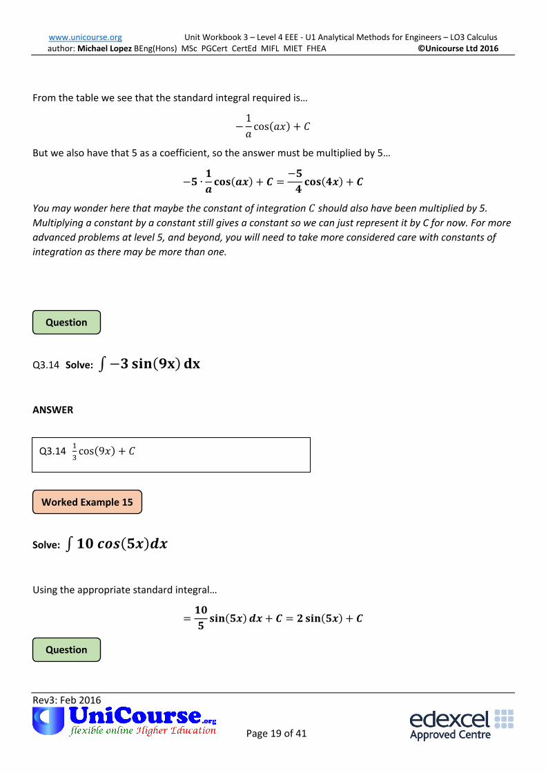
From the table we see that the standard integral required is…
−1
𝑎cos(𝑎𝑥) + 𝐶
But we also have that 5 as a coefficient, so the answer must be multiplied by 5…
−𝟓 ∙𝟏
𝒂𝐜𝐨𝐬(𝒂𝒙) + 𝑪 =
−𝟓
𝟒𝐜𝐨𝐬(𝟒𝒙) + 𝑪
You may wonder here that maybe the constant of integration 𝐶 should also have been multiplied by 5.
Multiplying a constant by a constant still gives a constant so we can just represent it by C for now. For more
advanced problems at level 5, and beyond, you will need to take more considered care with constants of
integration as there may be more than one.
Q3.14 Solve: ∫−𝟑 𝐬𝐢𝐧(𝟗𝐱)𝐝𝐱
ANSWER
Solve: ∫𝟏𝟎 𝒄𝒐𝒔(𝟓𝒙)𝒅𝒙
Using the appropriate standard integral…
=𝟏𝟎
𝟓𝐬𝐢𝐧(𝟓𝒙)𝒅𝒙 + 𝑪 = 𝟐𝐬𝐢𝐧(𝟓𝒙) + 𝑪
Q3.14 1
3cos(9𝑥) + 𝐶

www.unicourse.org Unit Workbook 3 – Level 4 EEE - U1 Analytical Methods for Engineers – LO3 Calculus author: Michael Lopez BEng(Hons) MSc PGCert CertEd MIFL MIET FHEA ©Unicourse Ltd 2016
Rev3: Feb 2016
Page 20 of 41 20 of 41
Worked Example 16
Question
Worked Example 17
Question
Q3.15 Solve: ∫𝟑𝟎 𝒄𝒐𝒔(𝟔𝒙)𝒅𝒙
Solve: ∫𝟐𝟒𝒆𝟖𝒙𝒅𝒙
Using the appropriate standard integral…
=𝟐𝟒
𝟖𝒆𝟖𝒙 + 𝑪 = 𝟑𝒆𝟖𝒙 + 𝑪
Q3.16 Solve: ∫𝟔𝒆𝟐𝒙𝒅𝒙
ANSWER
Solve: ∫𝟔
𝒙𝒅𝒙
Using the appropriate standard integral…
= 𝟔 𝒍𝒐𝒈𝒆(𝒙) + 𝑪
Q3.15 5 sin(6𝑥) + 𝐶
Q3.16 3𝑒2𝑥 + 𝐶
www.unicourse.org Unit Workbook 3 – Level 4 EEE - U1 Analytical Methods for Engineers – LO3 Calculus author: Michael Lopez BEng(Hons) MSc PGCert CertEd MIFL MIET FHEA ©Unicourse Ltd 2016
Rev3: Feb 2016
Page 21 of 41 21 of 41
Worked Example 18
Question
Question
Q3.17 Solve: ∫𝟗
𝒙𝒅𝒙
ANSWER
Solve: ∫(𝟖 𝐬𝐢𝐧𝐡(𝟒𝒙) + 𝟏𝟐 𝐜𝐨𝐬𝐡 (𝟔𝒙))𝒅𝒙
Here we have a sum of two functions. That’s not a problem, we just treat them as individual terms, find the
appropriate standard integrals, and add the results of the integration…
=8
4cosh(4𝑥) +
12
6sinh(6𝑥) + 𝐶 = 2 cosh(4𝑥) + 2 sinh(6𝑥) + 𝐶
You could then possibly go on to simplify this answer…
= 𝟐[𝐜𝐨𝐬𝐡(𝟒𝒙) + 𝐬𝐢𝐧𝐡 (𝟔𝒙)] + 𝑪
Q3.18 Solve: ∫(𝟔 𝐬𝐢𝐧𝐡(𝟑𝒙) + 𝟗 𝐜𝐨𝐬𝐡 (𝟒𝒙))𝒅𝒙
ANSWER
Perhaps you could try a more involved combination problem…
Q3.17 9 𝑙𝑜𝑔𝑒(𝑥) + 𝐶
Q3.18 2 cosh(3𝑥) +9
4sinh(4𝑥) + 𝐶

www.unicourse.org Unit Workbook 3 – Level 4 EEE - U1 Analytical Methods for Engineers – LO3 Calculus author: Michael Lopez BEng(Hons) MSc PGCert CertEd MIFL MIET FHEA ©Unicourse Ltd 2016
Rev3: Feb 2016
Page 22 of 41 22 of 41
Q3.19 Solve: ∫(−𝟑𝒙−𝟔 + 𝟒𝐬𝐢𝐧(𝟐𝒙) + 𝟖𝒆𝟒𝒙 + 𝟔 𝐬𝐢𝐧𝐡 (𝟑𝒙))𝒅𝒙
ANSWER
3.1.8 Definite Integrals and Areas under Curves In the previous section we mentioned that indefinite integrals do not have any limits imposed upon them.
In the case where there are limits imposed on an integral we call this a definite integral. These definite
integrals are useful for finding the area under a curve or function.
Let’s consider a nice simple function and see if we can work out the area beneath it between some given
limits. Suppose we take the function…
𝑦 = 2𝑥
We wish to find the area under that function for extremes of 𝑥 between 3 and 5. Here’s the idea…
The notation we use for such a case of definite integration is…
∫ 2𝑥 𝑑𝑥5
3
Notice that the lower limit (3) of the variable 𝑥 is placed at the lower end of the summation symbol and the
upper limit (5) is placed at the upper end of the summation symbol.
Another good thing to notice here is the use of that word ‘summation’. Looking at the graph for the
function it is clear that the area under the curve between our two limits (shown shaded) is a summation of
the area of the bit at the top, which looks like a triangle, and the lower bit, which looks like a rectangle.
You are probably thinking that you can work out that area in your head. If you did it would evaluate as 4
square units for the triangle and 12 square units for the rectangle, giving a total shaded area of 16 square
units. The actual summation for the integration is not done in chunks like that, it’s done as a sum of areas
moving horizontally, but the idea is the same.
Q3.19 3
5𝑥−5 − 2 cos(2𝑥) + 2𝑒4𝑥 + 2 cosh(3𝑥) + 𝐶

www.unicourse.org Unit Workbook 3 – Level 4 EEE - U1 Analytical Methods for Engineers – LO3 Calculus author: Michael Lopez BEng(Hons) MSc PGCert CertEd MIFL MIET FHEA ©Unicourse Ltd 2016
Rev3: Feb 2016
Page 23 of 41 23 of 41
Worked Example 19
Let’s see if we can perform our definite integration to arrive at the same answer.
∫ 2𝑥 𝑑𝑥5
3
= [2𝑥2
2]3
5
= [
𝑥2
]3
5
What we now do with our limits is place them into the variable in turn, separating each term with a ‘minus’
sign…
∫ 2𝑥 𝑑𝑥5
3
= [2𝑥2
2]3
5
= [
𝑥2
]3
5
= 52 − 32 = 25 − 9 = 16 𝑠𝑞𝑢𝑎𝑟𝑒 𝑢𝑛𝑖𝑡𝑠
You will notice that the constant of integration 𝐶 has not appeared here. It’s not that it was forgotten, in
fact it appeared twice, but that minus sign cancelled out those two 𝐶′𝑠.
That function 𝑦 = 2𝑥 was a straightforward one to visualise between horizontal limits. Let’s take a look at
one involving a sine wave…
Given the function 𝒚 = 𝐬𝐢𝐧 (𝒙) find the area under this function, bounded by limits of 𝒙 between 𝟎 and
𝝅.
Let’s go straight into this solution with our definite integral…
∫ sin(𝑥) 𝑑𝑥 = [
− cos (𝑥)
]0
𝜋
= (− cos (𝜋) − (− cos(0)) = 1 + 1 = 2 𝑠𝑞𝑢𝑎𝑟𝑒 𝑢𝑛𝑖𝑡𝑠𝜋
0
That one needed a lot of care with those minus signs. Let’s see how it looks graphically…

www.unicourse.org Unit Workbook 3 – Level 4 EEE - U1 Analytical Methods for Engineers – LO3 Calculus author: Michael Lopez BEng(Hons) MSc PGCert CertEd MIFL MIET FHEA ©Unicourse Ltd 2016
Rev3: Feb 2016
Page 24 of 41 24 of 41
Question
Q3.20 Given the function 𝒚 = 𝐜𝐨𝐬 (𝒙) find the area under this function, bounded by limits of 𝒙
between 𝟎 and 𝝅 𝟐⁄ .
ANSWER
Q3.20 1 square unit

www.unicourse.org Unit Workbook 3 – Level 4 EEE - U1 Analytical Methods for Engineers – LO3 Calculus author: Michael Lopez BEng(Hons) MSc PGCert CertEd MIFL MIET FHEA ©Unicourse Ltd 2016
Rev3: Feb 2016
Page 25 of 41 25 of 41
Worked Example 20
3.2 Further Differentiation
3.2.1 Higher Derivatives So far we have differentiated functions only once. When we differentiate a function more than once we
are finding higher derivatives of that function. At this point it is useful to introduce some shorthand
notation…
𝑑𝑦
𝑑𝑥≡ 𝑓′(𝑥)
Those three bars mean ‘equivalent to’. So, 𝑓′(𝑥) is a shorthand way of writing 𝑑𝑦 𝑑𝑥⁄ . Another piece of
more succinct shorthand is to use 𝑦′ as the first derivative of a function 𝑦. We may use these notations
interchangeably, therefore…
𝑑𝑦
𝑑𝑥≡ 𝑓′(𝑥) ≡ 𝑦′
When a function is differentiated for a second time we are saying…
𝑑 {𝑑𝑦𝑑𝑥}
𝑑𝑥
In other words, we are differentiating the contents of the curly brackets with respect to 𝑥. That doesn’t
look to good though, does it? The generally accepted ways to write this second derivative are…
𝑑2𝑦
𝑑𝑥2≡ 𝑓′′(𝑥) ≡ 𝑦′′
Each ‘dash’ represents a differentiation step. Therefore, a function which is differentiated 3 times can be
indicated in either of the following 3 ways…
𝑑3𝑦
𝑑𝑥3≡ 𝑓′′′(𝑥) ≡ 𝑦′′′
Let’s take a look at an example of taking higher derivatives…
Given the function 𝒚 = 𝟒𝒙𝟑 + 𝟑𝒆𝟐𝒙 + 𝟓 𝐬𝐢𝐧(𝟑𝐱) find 𝑦′′.
If you have worked through all of the previous examples and questions then you will have no problem at all
in being able to tackle such a question. Let’s get into the solution…
Firstly, we need to find 𝑦′…
𝑦′ = 12𝑥2 + 6𝑒2𝑥 + 15 cos (3𝑥)

www.unicourse.org Unit Workbook 3 – Level 4 EEE - U1 Analytical Methods for Engineers – LO3 Calculus author: Michael Lopez BEng(Hons) MSc PGCert CertEd MIFL MIET FHEA ©Unicourse Ltd 2016
Rev3: Feb 2016
Page 26 of 41 26 of 41
Question
Easy enough. If we now take the derivative of what we just found we shall have 𝑦′′…
𝒚′′ = 𝟐𝟒𝒙 + 𝟏𝟐𝒆𝟐𝒙 − 𝟒𝟓 𝐬𝐢𝐧 (𝟑𝒙)
Q3.21 Given the function 𝒚 = 𝟔𝒙𝟐 + 𝟐𝒆𝟔𝒙 − 𝟒 𝐜𝐨𝐬(𝟓𝐱) find 𝑦′′.
ANSWER
3.2.2 Logarithmic Differentiation When functions get quite complex it is frequently convenient to take natural logarithms of all the terms
before the process of differentiation takes place. Let’s review the three basic laws of logarithms in their
natural form…
𝒍𝒐𝒈𝒆(𝑨𝑩) = 𝒍𝒐𝒈𝒆(𝑨) + 𝒍𝒐𝒈𝒆(𝑩)
𝒍𝒐𝒈𝒆 (𝑨
𝑩) = 𝒍𝒐𝒈𝒆(𝑨) − 𝒍𝒐𝒈𝒆(𝑩)
𝒍𝒐𝒈𝒆(𝑨𝒏) = 𝒏 𝒍𝒐𝒈𝒆(𝑨)
As well as using those log laws we also need to understand a couple of important formulae before we can
use logarithmic differentiation. Consider the problem of differentiating 𝑦 = 𝑙𝑜𝑔𝑒(4𝑥3 + 3𝑥 − 6) with
respect to 𝑥. Our 𝑓(𝑥) here is 4𝑥3 + 3𝑥 − 6.
You will, of course, realise that this is a ‘function of a function’ type of problem…
𝐿𝑒𝑡 𝑢 = 4𝑥3 + 3𝑥 − 6 ∴ 𝑑𝑢
𝑑𝑥= 12𝑥2 + 3
𝐴𝑙𝑠𝑜, 𝑦 = 𝑙𝑜𝑔𝑒(𝑢) ∴ 𝑑𝑦
𝑑𝑢=1
𝑢
𝐶𝑜𝑙𝑙𝑒𝑐𝑡 𝑟𝑒𝑠𝑢𝑙𝑡𝑠: 𝑑𝑦
𝑑𝑥=𝑑𝑢
𝑑𝑥∙𝑑𝑦
𝑑𝑢=12𝑥2 + 3
𝑢=
12𝑥2 + 3
4𝑥3 + 3𝑥 − 6
That last result looks like 𝑓′(𝑥) 𝑓(𝑥)⁄ . So, our first important result is…
𝒅
𝒅𝒙[𝒍𝒐𝒈𝒆(𝒇(𝒙))] =
𝒇′(𝒙)
𝒇(𝒙)
Q3.21 12 + 72𝑒6𝑥 + 100 cos(5𝑥)

www.unicourse.org Unit Workbook 3 – Level 4 EEE - U1 Analytical Methods for Engineers – LO3 Calculus author: Michael Lopez BEng(Hons) MSc PGCert CertEd MIFL MIET FHEA ©Unicourse Ltd 2016
Rev3: Feb 2016
Page 27 of 41 27 of 41
Worked Example 21
On to our second important result then…
If we are given 𝑙𝑜𝑔𝑒(𝑦) and are asked to differentiate it with respect to 𝑥 then that is not the type of
problem which we have met before. All of our problems so far have involved explicit functions, where we
would have been given something like 𝑦 = 𝑓(𝑥). That’s not the case here. In fact, what we are currently
given is called an implicit function. Here’s how we go about differentiating 𝑙𝑜𝑔𝑒(𝑦) with respect to the
implicit variable 𝑥…
𝐹𝑖𝑛𝑑 𝑑
𝑑𝑥{𝑙𝑜𝑔𝑒(𝑦)}
𝐿𝑒𝑡 𝑢 = 𝑙𝑜𝑔𝑒(𝑦) ∴ 𝑑𝑢
𝑑𝑦=1
𝑦
𝑅𝑒𝑎𝑙𝑖𝑠𝑖𝑛𝑔 𝑡ℎ𝑎𝑡: 𝑑𝑢
𝑑𝑥=𝑑𝑢
𝑑𝑦∙𝑑𝑦
𝑑𝑥 ∴
𝑑
𝑑𝑥{𝑙𝑜𝑔𝑒(𝑦)} =
1
𝑦∙𝑑𝑦
𝑑𝑥
Let’s just emphasise that last result…
𝒅
𝒅𝒙{𝒍𝒐𝒈𝒆(𝒚)} =
𝟏
𝒚∙𝒅𝒚
𝒅𝒙
We are now in a position to be able to perform logarithmic differentiation.
There are plenty of problems where using the Product Rule, Quotient Rule etc. sends us to a dead end. This
is usually where logarithmic differentiation comes to the fore. Consider differentiating the following
function with respect to 𝑥…
𝑦 =𝑥2cosh (𝑥)
𝑒4𝑥sin (𝑥)
Wow, that looks complicated. Below is a section of the function drawn in Graph (on the left) and the
function along with the derivative (in red and blue respectively, on the right). Our job is to produce an
equation for that blue curve.
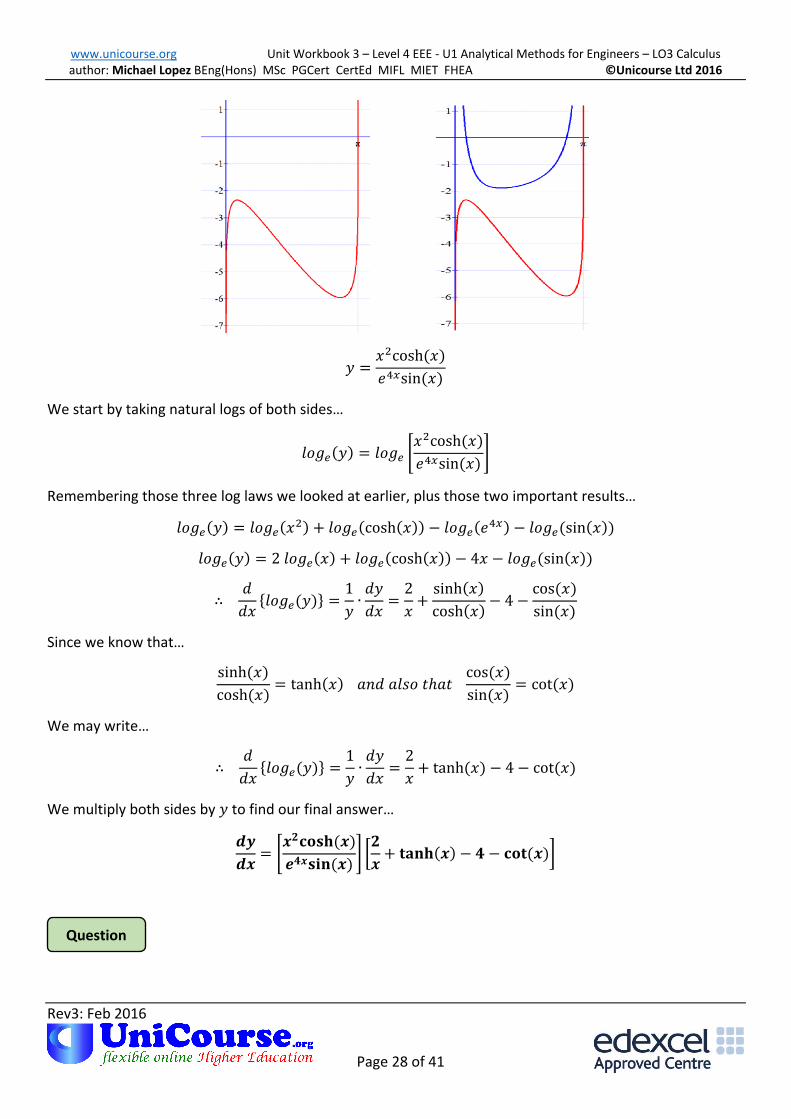
www.unicourse.org Unit Workbook 3 – Level 4 EEE - U1 Analytical Methods for Engineers – LO3 Calculus author: Michael Lopez BEng(Hons) MSc PGCert CertEd MIFL MIET FHEA ©Unicourse Ltd 2016
Rev3: Feb 2016
Page 28 of 41 28 of 41
Question
𝑦 =𝑥2cosh (𝑥)
𝑒4𝑥sin (𝑥)
We start by taking natural logs of both sides…
𝑙𝑜𝑔𝑒(𝑦) = 𝑙𝑜𝑔𝑒 [𝑥2cosh (𝑥)
𝑒4𝑥sin (𝑥)]
Remembering those three log laws we looked at earlier, plus those two important results…
𝑙𝑜𝑔𝑒(𝑦) = 𝑙𝑜𝑔𝑒(𝑥2) + 𝑙𝑜𝑔𝑒(cosh(𝑥)) − 𝑙𝑜𝑔𝑒(𝑒
4𝑥) − 𝑙𝑜𝑔𝑒(sin(𝑥))
𝑙𝑜𝑔𝑒(𝑦) = 2 𝑙𝑜𝑔𝑒(𝑥) + 𝑙𝑜𝑔𝑒(cosh(𝑥)) − 4𝑥 − 𝑙𝑜𝑔𝑒(sin(𝑥))
∴ 𝑑
𝑑𝑥{𝑙𝑜𝑔𝑒(𝑦)} =
1
𝑦∙𝑑𝑦
𝑑𝑥=2
𝑥+sinh(𝑥)
cosh(𝑥)− 4 −
cos (𝑥)
sin (𝑥)
Since we know that…
sinh (𝑥)
cosh (𝑥)= tanh(𝑥) 𝑎𝑛𝑑 𝑎𝑙𝑠𝑜 𝑡ℎ𝑎𝑡
cos (𝑥)
sin (𝑥)= cot (𝑥)
We may write…
∴ 𝑑
𝑑𝑥{𝑙𝑜𝑔𝑒(𝑦)} =
1
𝑦∙𝑑𝑦
𝑑𝑥=2
𝑥+ tanh (𝑥) − 4 − cot (𝑥)
We multiply both sides by 𝑦 to find our final answer…
𝒅𝒚
𝒅𝒙= [𝒙𝟐𝐜𝐨𝐬𝐡 (𝒙)
𝒆𝟒𝒙𝐬𝐢𝐧 (𝒙)] [𝟐
𝒙+ 𝐭𝐚𝐧𝐡(𝒙) − 𝟒 − 𝐜𝐨𝐭 (𝒙)]

www.unicourse.org Unit Workbook 3 – Level 4 EEE - U1 Analytical Methods for Engineers – LO3 Calculus author: Michael Lopez BEng(Hons) MSc PGCert CertEd MIFL MIET FHEA ©Unicourse Ltd 2016
Rev3: Feb 2016
Page 29 of 41 29 of 41
Q3.22 Differentiate the following function with respect to 𝒙…
𝒚 = 𝟑𝒙 𝐬𝐢𝐧(𝒙) 𝐜𝐨𝐬 (𝒙)
ANSWER
3.2.3 Differentiation of Inverse Trigonometric Functions Suppose we have the equation…
𝑦 = 𝑠𝑖𝑛−1(𝑥)
How do we then go about finding 𝑑𝑦 𝑑𝑥⁄ ? Maybe we should write this in a different form…
𝑥 = sin(𝑦)
Now can differentiate…
𝑑𝑥
𝑑𝑦= cos(𝑦) ∴ 𝑓𝑙𝑖𝑝 𝑏𝑜𝑡ℎ 𝑠𝑖𝑑𝑒𝑠:
𝑑𝑦
𝑑𝑥=
1
cos (𝑦)
Next we shall remember one of our handy trig. Identities…
𝑐𝑜𝑠2(𝑦) + 𝑠𝑖𝑛2(𝑦) = 1 ∴ 𝑐𝑜𝑠2(𝑦) = 1 − 𝑠𝑖𝑛2(𝑦) ∴ cos(𝑦) = √1 − 𝑠𝑖𝑛2(𝑦)
Since we know 𝑥 = sin(𝑦) then if we square both sides we shall have 𝑥2 = 𝑠𝑖𝑛2(𝑦)
So we may re-write our transposed trig. identity as…
cos(𝑦) = √1 − 𝑥2
Now we can put this latest result back into our differential…
𝒅𝒚
𝒅𝒙=
𝟏
𝐜𝐨𝐬 (𝒚)=
𝟏
√𝟏 − 𝒙𝟐=
𝟏
(𝟏 − 𝒙𝟐)𝟎.𝟓= (𝟏 − 𝒙𝟐)−𝟎.𝟓
That was a bit tricky, but we managed to find 𝑦′.
Let’s go on and see if we can find 𝑦′′…
𝑦′ = (1 − 𝑥2)−0.5
Q3.22 [3𝑥 𝑠𝑖𝑛(𝑥) cos (𝑥)] [ 1
𝑥+ cot(𝑥) − tan (𝑥)]
www.unicourse.org Unit Workbook 3 – Level 4 EEE - U1 Analytical Methods for Engineers – LO3 Calculus author: Michael Lopez BEng(Hons) MSc PGCert CertEd MIFL MIET FHEA ©Unicourse Ltd 2016
Rev3: Feb 2016
Page 30 of 41 30 of 41
Question
This is where that shorthand notation for derivatives comes in really handy…
𝐿𝑒𝑡 𝑢 = 1 − 𝑥2 ∴ 𝑑𝑢
𝑑𝑥= −2𝑥
∴ 𝑦′ = 𝑢−0.5
∴ 𝑑𝑦′
𝑑𝑢= −0.5𝑢−1.5
∴ 𝑦′′ =𝑑𝑢
𝑑𝑥∙ 𝑑𝑦′
𝑑𝑢= −2𝑥 × −0.5𝑢−1.5
∴ 𝒚′′ = 𝒙𝒖−𝟏.𝟓 = 𝒙(𝟏 − 𝒙𝟐)−𝟏.𝟓
Q3.23 Find 𝒚′′ for 𝒚 = 𝒄𝒐𝒔−𝟏(𝟐𝒙)
ANSWER
3.2.4 Differentiation of Inverse Hyperbolic Functions Consider the function…
𝑦 = 𝑠𝑖𝑛ℎ−1(𝑥)
Our task here is to find 𝑦′′. We proceed in a similar manner to the previous problem…
𝑥 = sinh (𝑦)
∴ 𝑑𝑥
𝑑𝑦= cosh(𝑦) ∴
𝑑𝑦
𝑑𝑥=
1
cosh (𝑦)
A useful identity is…
𝑐𝑜𝑠ℎ2(𝑦) − 𝑠𝑖𝑛ℎ2(𝑦) = 1 ∴ 𝑐𝑜𝑠ℎ2(𝑦) = 1 + 𝑠𝑖𝑛ℎ2(𝑦)
∴ 𝑐𝑜𝑠ℎ2(𝑦) = 1 + 𝑥2 ∴ cosh(𝑦) = √1 + 𝑥2
∴ 𝒅𝒚
𝒅𝒙= 𝒚′ =
𝟏
√𝟏 + 𝒙𝟐= (𝟏 + 𝒙𝟐)−𝟎.𝟓
Q3.23 −8𝑥
(1−4𝑥2)1.5

www.unicourse.org Unit Workbook 3 – Level 4 EEE - U1 Analytical Methods for Engineers – LO3 Calculus author: Michael Lopez BEng(Hons) MSc PGCert CertEd MIFL MIET FHEA ©Unicourse Ltd 2016
Rev3: Feb 2016
Page 31 of 41 31 of 41
Question
Now to find that second derivative…
𝑦′ = (1 + 𝑥2)−0.5
𝐿𝑒𝑡 𝑢 = 1 + 𝑥2 ∴ 𝑑𝑢
𝑑𝑥= 2𝑥
∴ 𝑦′ = 𝑢−0.5 ∴ 𝑑𝑦′
𝑑𝑢= −0.5𝑢−1.5
∴ 𝑦′′ =𝑑𝑢
𝑑𝑥∙ 𝑑𝑦′
𝑑𝑢= 2𝑥 × −0.5𝑢−1.5 = −𝑥(1 + 𝑥2)−1.5
Q3.24 Find 𝒚′′ for 𝒚 = 𝒄𝒐𝒔𝒉−𝟏(𝟐𝒙)
ANSWER
Q3.24 −8𝑥
(4𝑥2−1)1.5

www.unicourse.org Unit Workbook 3 – Level 4 EEE - U1 Analytical Methods for Engineers – LO3 Calculus author: Michael Lopez BEng(Hons) MSc PGCert CertEd MIFL MIET FHEA ©Unicourse Ltd 2016
Rev3: Feb 2016
Page 32 of 41 32 of 41
3.3 Further Integration
3.3.1 Integration by Parts This technique provides us with a way to integrate the product of two simple functions. We shall develop a
formula to use as a framework for the technique.
The starting point for our formula lies with the Product Rule, which you mastered in Section 3.1.5…
𝑑
𝑑𝑥(𝑢𝑣) = 𝑢
𝑑𝑣
𝑑𝑥+ 𝑣
𝑑𝑢
𝑑𝑥
Let’s rearrange this formula…
𝑢𝑑𝑣
𝑑𝑥=𝑑
𝑑𝑥(𝑢𝑣) − 𝑣
𝑑𝑢
𝑑𝑥
If we now integrate both sides with respect to 𝑥 then we need to place a ∫ sign before each term and a 𝑑𝑥
at the end of each term, like so…
∫𝑢𝑑𝑣
𝑑𝑥𝑑𝑥 = ∫
𝑑
𝑑𝑥(𝑢𝑣)𝑑𝑥 − ∫𝑣
𝑑𝑢
𝑑𝑥𝑑𝑥
Some simplifications can be noticed here:
In the first integral the two 𝑑𝑥 terms cancel each other out
In the second integral we are taking the ‘integral of the differential’ of 𝑢𝑣. Since integration is the
reverse of differentiation then the ’integral of a differential’ drops away, just leaving 𝑢𝑣
In the third integral the two 𝑑𝑥 terms cancel each other out
Performing these simplifications gives…
∫𝒖 𝒅𝒗 = 𝒖𝒗 −∫𝒗 𝒅𝒖
That is our formula for integration by parts.
What we do with the formula is to look at the left hand side and see the integral of a product. That product
is composed of 𝑢 and 𝑑𝑣. When using integration by parts you have a choice of which part of the product
to call 𝑢 and which to call 𝑑𝑣. Fortunately, your choice is guided…
The 𝑢 part will become a constant after taking multiple derivatives
The 𝑑𝑣 part is readily integrated by using standard integrals.
www.unicourse.org Unit Workbook 3 – Level 4 EEE - U1 Analytical Methods for Engineers – LO3 Calculus author: Michael Lopez BEng(Hons) MSc PGCert CertEd MIFL MIET FHEA ©Unicourse Ltd 2016
Rev3: Feb 2016
Page 33 of 41 33 of 41
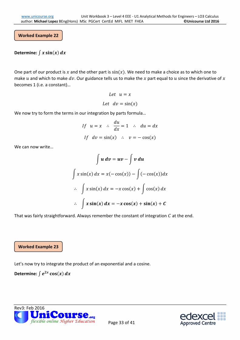
Worked Example 22
Worked Example 23
Determine: ∫𝒙 𝐬𝐢𝐧(𝒙)𝒅𝒙
One part of our product is 𝑥 and the other part is sin (𝑥). We need to make a choice as to which one to
make 𝑢 and which to make 𝑑𝑣. Our guidance tells us to make the 𝑥 part equal to 𝑢 since the derivative of 𝑥
becomes 1 (i.e. a constant)…
𝐿𝑒𝑡 𝑢 = 𝑥
𝐿𝑒𝑡 𝑑𝑣 = sin (𝑥)
We now try to form the terms in our integration by parts formula…
𝐼𝑓 𝑢 = 𝑥 ∴ 𝑑𝑢
𝑑𝑥= 1 ∴ 𝑑𝑢 = 𝑑𝑥
𝐼𝑓 𝑑𝑣 = sin(𝑥) ∴ 𝑣 = − cos (𝑥)
We can now write…
∫𝒖 𝒅𝒗 = 𝒖𝒗 −∫𝒗 𝒅𝒖
∫𝑥 sin(𝑥) 𝑑𝑥 = 𝑥(− cos(𝑥)) − ∫(− cos(𝑥))𝑑𝑥
∴ ∫ 𝑥 sin(𝑥) 𝑑𝑥 = −𝑥 cos(𝑥) + ∫cos(𝑥) 𝑑𝑥
∴ ∫𝒙 𝐬𝐢𝐧(𝒙) 𝒅𝒙 = −𝒙𝐜𝐨𝐬(𝒙) + 𝐬𝐢𝐧(𝒙) + 𝑪
That was fairly straightforward. Always remember the constant of integration 𝐶 at the end.
Let’s now try to integrate the product of an exponential and a cosine.
Determine: ∫𝒆𝟐𝒙 𝐜𝐨𝐬(𝒙) 𝒅𝒙

www.unicourse.org Unit Workbook 3 – Level 4 EEE - U1 Analytical Methods for Engineers – LO3 Calculus author: Michael Lopez BEng(Hons) MSc PGCert CertEd MIFL MIET FHEA ©Unicourse Ltd 2016
Rev3: Feb 2016
Page 34 of 41 34 of 41
Our two products here are 𝑒2𝑥 and cos (𝑥). Neither of them will reduce to a constant when differentiated
so it doesn’t matter which one we call 𝑢 and which we call 𝑑𝑣. You will see here that we need to do
integration by parts twice to arrive at our answer.
Just as in the previous worked example we need to decide on assignments for 𝑢 and 𝑑𝑣, then find 𝑣 and
𝑑𝑢. Let’s do that…
𝐿𝑒𝑡 𝑢 = 𝑒2𝑥 ∴ 𝑑𝑢
𝑑𝑥= 2𝑒2𝑥 ∴ 𝑑𝑢 = 2𝑒2𝑥𝑑𝑥
𝐿𝑒𝑡 𝑑𝑣 = cos(𝑥) ∴ 𝑣 = sin (𝑥)
To aid our working here (and save some ink) we normally assign the capital letter 𝐼 to the integral in our
question.
∴ 𝐼 = ∫𝑒2𝑥 cos(𝑥) 𝑑𝑥
∴ 𝐼 = 𝑒2𝑥 sin(𝑥) − ∫sin(𝑥) 2𝑒2𝑥𝑑𝑥
This needs tidying…
∴ 𝐼 = 𝑒2𝑥 sin(𝑥) − 2∫𝑒2𝑥sin(𝑥) 𝑑𝑥
We were rather hoping for an answer, but what we seem to have is another ‘integration by parts’ problem
embedded into our development. Don’t worry, that’s quite normal for this type of problem. All we do is
attack that last part with ‘integration by parts’ once more, using square brackets. Our desired result will
then appear…
𝐼 = 𝑒2𝑥 sin(𝑥) − 2 [𝑒2𝑥(−cos (𝑥)) − ∫−cos (𝑥)2𝑒2𝑥𝑑𝑥]
Expanding these terms gives…
𝐼 = 𝑒2𝑥 sin(𝑥) + 2𝑒2𝑥 cos(𝑥) − 4∫𝑒2𝑥 cos(𝑥) 𝑑𝑥
That last integral is the same as 𝐼, which is really handy, so we may now write…
𝐼 = 𝑒2𝑥 sin(𝑥) + 2𝑒2𝑥 cos(𝑥) − 4𝐼
∴ 5𝐼 = 𝑒2𝑥 sin(𝑥) + 2𝑒2𝑥cos (𝑥)
If we divide both sides by 5 then we have our final answer…

www.unicourse.org Unit Workbook 3 – Level 4 EEE - U1 Analytical Methods for Engineers – LO3 Calculus author: Michael Lopez BEng(Hons) MSc PGCert CertEd MIFL MIET FHEA ©Unicourse Ltd 2016
Rev3: Feb 2016
Page 35 of 41 35 of 41
Question
Worked Example 24
𝑰 =𝒆𝟐𝒙 𝐬𝐢𝐧(𝒙) + 𝟐𝒆𝟐𝒙𝐜𝐨𝐬 (𝒙)
𝟓
Q3.25 Determine: ∫𝒆𝟒𝒙𝒔𝒊𝒏(𝟐𝒙)𝒅𝒙
ANSWER
3.3.2 Integration by Substitution Quite often we come across integrals which are a function of a linear algebraic function. To solve such
problems we introduce the variable 𝑢, as seen earlier, and make a convenient substitution with the
derivative of 𝑢. Let’s look at an example…
Determine: ∫(𝟑𝒙 − 𝟐)𝟓𝒅𝒙
This looks like an integration of a ‘function of a function’ problem. We know already how to find the
derivative of ‘function of a function’ problems, but now we learn how to find their integrals.
As mentioned, we shall introduce 𝑢 and make it equal to the contents of the brackets…
𝑢 = 3𝑥 − 2 ∴ 𝑑𝑢
𝑑𝑥= 3
We are going to find it useful to have an expression for 𝑑𝑥 𝑑𝑢⁄ . This is not a problem, we just need to flip
both sides…
∴ 𝑑𝑥
𝑑𝑢=1
3
Let’s now express our original problem in terms of 𝑢…
Q3.25 4𝑒4𝑥 sin(2𝑥)−2𝑒4𝑥cos(2𝑥)
20

www.unicourse.org Unit Workbook 3 – Level 4 EEE - U1 Analytical Methods for Engineers – LO3 Calculus author: Michael Lopez BEng(Hons) MSc PGCert CertEd MIFL MIET FHEA ©Unicourse Ltd 2016
Rev3: Feb 2016
Page 36 of 41 36 of 41
Question
Worked Example 25
∫𝑢5𝑑𝑥
We can’t solve that in its current form. What we need to do is to change the variable. Here’s the trick…
∫𝑢5𝑑𝑥 = ∫𝑢5𝑑𝑥
𝑑𝑢𝑑𝑢
Notice that those 𝑑𝑢 terms potentially cancel each other out, so what we have written is perfectly fine.
Another thing we notice here is that we actually know what 𝑑𝑥 𝑑𝑢⁄ is. We worked it out before as 1/3. We
can now write…
∫𝑢5𝑑𝑥 = ∫𝑢5𝑑𝑥
𝑑𝑢𝑑𝑢 =
1
3∫𝑢5𝑑𝑢 =
1
3∙𝑢6
6+ 𝐶 =
𝑢6
18+ 𝐶
If we now replace 𝑢 with its original value of (3𝑥 − 2) we shall arrive at our answer…
∫(𝟑𝒙 − 𝟐)𝟓𝒅𝒙 =(𝟑𝒙 − 𝟐)𝟔
𝟏𝟖+ 𝑪
Q3.26 Determine: ∫(𝟐𝒙 − 𝟔)𝟒𝒅𝒙
ANSWER
3.3.3 Integration using Partial Fractions Many functions must be expressed in terms of partial fractions before they can be integrated. Partial
fractions were covered in Workbook 1. Let’s take a look at an integration problem requiring the use of
partial fractions.
Determine:
∫𝒙𝟐
(𝒙 + 𝟐)(𝒙 − 𝟏)𝟐𝒅𝒙
Q3.26 (2𝑥−6)5
10+ 𝐶

www.unicourse.org Unit Workbook 3 – Level 4 EEE - U1 Analytical Methods for Engineers – LO3 Calculus author: Michael Lopez BEng(Hons) MSc PGCert CertEd MIFL MIET FHEA ©Unicourse Ltd 2016
Rev3: Feb 2016
Page 37 of 41 37 of 41
Question
We need to break the problem up into smaller fractions. Partial fractions are the result. Let’s use our
knowledge from Workbook 1 to determine these partial fractions.
𝑥2
(𝑥 + 2)(𝑥 − 1)2≡
𝐴
(𝑥 + 2)+
𝐵
(𝑥 − 1)+
𝐶
(𝑥 − 1)2
Now multiply both sides by (𝑥 + 2)(𝑥 − 1)2. This will give us a one line expression…
𝑥2 = 𝐴(𝑥 − 1)2 + 𝐵(𝑥 + 2)(𝑥 − 1) + 𝐶(𝑥 + 2)
𝐿𝑒𝑡 𝑥 = 1:
(1)2 = 3𝐶 ∴ 𝐶 = 1 3⁄
𝐿𝑒𝑡 𝑥 = −2:
(−2)2 = 9𝐴 ∴ 𝐴 = 4 9⁄
We now need to find 𝐵. One way to do that is to equate coefficients of 𝑥2…
[𝑥2]: 1 = 𝐴 + 𝐵
∴ 𝐵 = 1 − 𝐴 = 1 − 4 9⁄ = 5 9⁄
Since we now know the value of each of the three constants we may express the initial problem as…
∫𝑥2
(𝑥 + 2)(𝑥 − 1)2𝑑𝑥 = ∫(
49⁄
(𝑥 + 2)+
59⁄
(𝑥 − 1)+
13⁄
(𝑥 − 1)2)𝑑𝑥
The right hand side may be split into three integrals, as follows…
∫𝑥2
(𝑥 + 2)(𝑥 − 1)2𝑑𝑥 =
4
9∙ ∫
1
(𝑥 + 2)𝑑𝑥 +
5
9∙ ∫
1
(𝑥 − 1)𝑑𝑥 +
1
3∙ ∫
1
(𝑥 − 1)2𝑑𝑥
These three integrals on the right hand side may be evaluated as…
∫𝒙𝟐
(𝒙 + 𝟐)(𝒙 − 𝟏)𝟐𝒅𝒙 =
𝟒
𝟗𝒍𝒐𝒈𝒆(𝒙 + 𝟐) +
𝟓
𝟗𝒍𝒐𝒈𝒆(𝒙 − 𝟏) −
𝟏
𝟑𝒙 − 𝟑+ 𝑪
Q3.27 Determine:
∫𝒙𝟐
(𝒙 − 𝟐)(𝒙 + 𝟏)𝟐𝒅𝒙
www.unicourse.org Unit Workbook 3 – Level 4 EEE - U1 Analytical Methods for Engineers – LO3 Calculus author: Michael Lopez BEng(Hons) MSc PGCert CertEd MIFL MIET FHEA ©Unicourse Ltd 2016
Rev3: Feb 2016
Page 38 of 41 38 of 41
ANSWER
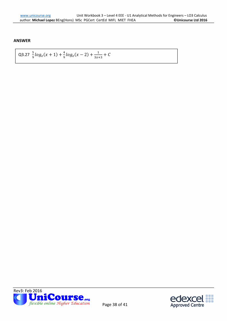
Q3.27 5
9𝑙𝑜𝑔𝑒(𝑥 + 1) +
4
9𝑙𝑜𝑔𝑒(𝑥 − 2) +
1
3𝑥+3+ 𝐶

www.unicourse.org Unit Workbook 3 – Level 4 EEE - U1 Analytical Methods for Engineers – LO3 Calculus author: Michael Lopez BEng(Hons) MSc PGCert CertEd MIFL MIET FHEA ©Unicourse Ltd 2016
Rev3: Feb 2016
Page 39 of 41 39 of 41
3.4 Solution of Engineering Problems with Calculus
3.4.1 Charging RC Circuit For the circuit below, use Calculus to find the charge stored in the capacitor 2 seconds after the switch
closes. Assume zero charge on the capacitor before this event.
For a capacitor charging via a DC source voltage, through a series resistor, the formula for instantaneous
current is…
𝑖 =𝐸
𝑅∙ 𝑒(
−𝑡𝑅𝐶⁄ ) 𝐴𝑚𝑝𝑠
Since current is the defined as the rate of change of charge (𝑞, carried by passing electrons) we may say…
𝑖 =𝑑𝑞
𝑑𝑡
If we integrate both sides with respect to 𝑡 we will have…
∫𝑖 𝑑𝑡 = ∫𝑑𝑞
𝑑𝑡 𝑑𝑡 = ∫𝑑𝑞 = 𝑞
So we may say that…
𝑞 = ∫ 𝑖 𝑑𝑡
If we wish to find the amount of charge store stored within a certain time period (i.e. 2 seconds in this
example) we write…
𝑞(0−2) = ∫ 𝑖 𝑑𝑡
2
0
= ∫𝐸
𝑅∙ 𝑒(
−𝑡𝑅𝐶⁄ )
2
0
𝑑𝑡
=𝐸
𝑅[𝑒{−1𝑅𝐶}𝑡
−1𝑅𝐶⁄]
0
2
=−𝐸𝑅𝐶
𝑅[𝑒(
−𝑡𝑅𝐶⁄ )]
0
2= −𝐸𝐶 [𝑒(
−𝑡𝑅𝐶⁄ )]
0
2

www.unicourse.org Unit Workbook 3 – Level 4 EEE - U1 Analytical Methods for Engineers – LO3 Calculus author: Michael Lopez BEng(Hons) MSc PGCert CertEd MIFL MIET FHEA ©Unicourse Ltd 2016
Rev3: Feb 2016
Page 40 of 41 40 of 41
Since we know that 𝑅 = 1𝑀Ω and 𝐶 = 1𝜇𝐹 then 𝑅𝐶 = 1 × 106 × 1 × 10−6 = 106−6 = 100 = 1 we may
write…
𝑞(0−2) = −𝐸𝐶 [𝑒(−𝑡 1⁄ )]
0
2= −𝐸𝐶[𝑒−𝑡]0
2 = −𝐸𝐶[𝑒−2 − 𝑒−0] = −𝐸𝐶[0.135 − 1]
We also know that the DC supply voltage (𝐸) is 10V…
∴ 𝒒(𝟎−𝟐) = −𝟏𝟎 × 𝟏 × 𝟏𝟎−𝟔[−𝟎. 𝟖𝟔𝟓] = 𝟖. 𝟔𝟓 × 𝟏𝟎−𝟔 𝑪𝒐𝒖𝒍𝒐𝒎𝒃𝒔 = 𝟖. 𝟔𝟓 𝝁𝑪
The plot below illustrates the integration we have just performed…
Current is on the vertical axis and time on the horizontal. When we multiply current by time we get charge,
which is shown as the shaded area between 0 and 2 seconds. You may like to experiment with the Graph
simulator to produce similar results.
3.4.2 Energising Inductor Consider the series RL circuit below…
If 𝑬 = 𝟏𝟎 𝑽, 𝑹 = 𝟏𝑴𝛀 and 𝑳 = 𝟐𝟎𝟎𝒎𝑯, use Calculus to determine the voltage across the inductor after
𝟎. 𝟏𝝁𝒔. Use the following formulae in your solution development…

www.unicourse.org Unit Workbook 3 – Level 4 EEE - U1 Analytical Methods for Engineers – LO3 Calculus author: Michael Lopez BEng(Hons) MSc PGCert CertEd MIFL MIET FHEA ©Unicourse Ltd 2016
Rev3: Feb 2016
Page 41 of 41 41 of 41
𝒊 =𝑬
𝑹(𝟏 − 𝒆
−𝑹𝒕𝑳⁄ ) 𝒂𝒏𝒅 𝒗𝑳 = 𝑳
𝒅𝒊
𝒅𝒕
We start with…
𝑣𝐿 = 𝐿𝑑𝑖
𝑑𝑡= 𝐿
𝑑 {𝐸𝑅(1 − 𝑒
−𝑅𝑡𝐿⁄ )}
𝑑𝑡
=𝐿𝐸
𝑅∙𝑑 (1 − 𝑒
−𝑅𝑡𝐿⁄ )
𝑑𝑡=𝐿𝐸
𝑅(𝑅
𝐿∙ 𝑒−𝑅𝑡
𝐿⁄ ) = 𝐸𝑒−𝑅𝑡
𝐿⁄
Putting in the values for E, R, t and L gives…
𝒗𝑳 = 𝟏𝟎𝒆(−𝟏𝟎𝟔×𝟎.𝟏×𝟏𝟎−𝟔
𝟎.𝟐 )= 𝟔. 𝟎𝟔𝟓 𝒗𝒐𝒍𝒕𝒔