Embed Size (px)
Citation preview
1
UNITED STATES ANTHROPOGENIC EMISSIONS RATE OF PROGRESS
1.0 INTRODUCTION
The United States anthropogenic emissions Rate of Progress (RoP) is an alternative approach to the
Uniform Rate of Progress (URP) Glidepath to estimate whether visibility impairment at Class I areas
(CIAs) is on a path toward no manmade impairment in 2064.
1.1 Overview
Photochemical grid model (PGM) source apportionment modeling is used to develop the United States
(U.S.) anthropogenic emissions RoP analysis to estimate the rate that visibility impairment due to U.S.
anthropogenic emissions is being reduced over time. The Comprehensive Air-quality Model with
extensions (CAMx) PGM simulations are conducted for a 2002 Hindcast year, a Representative Baseline
(RepBase2) current year (representing 2014-2018 conditions) and a 2028 future year (2028OTBa2). The
CAMx Particulate Source Apportionment Technology (PSAT) source apportionment tool is used to isolate
the contributions of U.S. anthropogenic emissions, along with other sources (e.g., International
anthropogenic emissions, fires and natural sources), to visibility extinction at IMPROVE monitoring sites
representing CIAs in the western U.S. This allows for the estimation of the changes in visibility
impairment due to U.S. anthropogenic emissions at CIAs over time and whether they are trending
toward no impairment due to U.S. anthropogenic emissions by 2064.
A second use of the CAMx 2002 Hindcast simulation is for a Dynamic Evaluation that evaluates the
model’s ability to predict a change in visibility due to a change in emissions using the same procedures
as used to make future year 2028 visibility projections. The future year 2028 visibility projection
procedures use the relative change in modeling results between current (RepBase2) and future
(2028OTBa2) year conditions to scale the observed current year (2014-2018) visibility conditions for the
IMPROVE 20% Most Impaired Days (MID) to estimate the 2028 MID visibility conditions. The Dynamic
Evaluation compares the modeled projected and observed changes in visibility between the 2000-2004
Baseline and the 2014-2018 current 5-year planning period for the IMPROVE MID.
1.2 Webpage Organization
This webpage is organized into four major sections as follows:
1. Introduction: Provides an overview, background and purpose of the analysis.
2. U.S. Anthropogenic Emissions Rate of Progress: Results of the modeled U.S. anthropogenic
emissions RoP and whether the modeled U.S. anthropogenic emissions impairment at CIAs in
2028 are on a path toward no U.S. manmade impairment in 2064.
3. Dynamic Evaluation: Evaluates the WRAP 2028 visibility projection procedures by using the
CAMx current year (RepBase) and 2002 Hindcast modeling results to make visibility projections
that are compared with the observed 2000-2004 and 2014-2018 IMPROVE MID visibility
conditions.
4. CAMx 2002 Hindcast Simulation Development: The assumptions and procedures used for
making the CAMx 2002 Hindcast simulation are presented in the last major section of this
webpage.
1.3 Regional Haze Rule Objectives
2
The main objective of the Regional Haze Rule (RHR) is to mitigate manmade visibility impairment at CIAs.
There are 156 CIAs that consists of national parks and wilderness areas with a vast majority of them
located in the western U.S. As part of the development of the second round of Regional Haze Rule
(RHR) State Implementation Plans (SIPs), states need show that reasonable progress is being made
toward natural conditions to be achieved by 2064 (EPA, 2016). EPA has recently developed a new Most
Impaired Days (MID) visibility metric based on measured PM species concentrations at IMPROVE
monitoring sites that is the recommended metric for tracking visibility progress toward natural
conditions (EPA, 2018). The EPA method for identifying the IMPROVE MID uses a statistical procedure
that is designed to identify days at IMPROVE monitoring sites that are likely to be most impaired by
anthropogenic emissions, primarily relying on the assumption that measured extinction due to
ammonium sulfate (AmmSO4) and ammonium nitrate (AmmNO3) are primarily from manmade
emissions. Using the IMPROVE sampling record from 2000-2014, the IMPROVE MID statistical
procedure estimates the contributions of routine natural haze and natural haze due to episodic events
using measured light extinction due to carbon and geogenic species as proxies for impacts due to,
respectively, wildfires and windblown dust (WBD) with the remainder of the extinction assumed to be
mainly anthropogenic in origin. The IMPROVE MID visibility metric is obtained for each year as the 20%
days with highest anthropogenic visibility impairment after the statistical procedures have identified the
natural components due to fire and dust contributions from carbon and geogenic filter mass
measurements. The IMPROVE MID is the metric required in the procedure recommended by EPA to
evaluate progress for the 2028 planning milestone toward reaching the distant long-term goal of
achieving estimated natural conditions at CIAs by 2064 (EPA, 2018).
To help assess whether a CIA is on a path toward this RHR long-term goal, the trends in the IMPROVE
MID visibility impairment are compared against the URP Glidepath that is obtained as a straight line
trend in visibility (in deciview, dv) from the measured IMPROVE MID from the 2000-2004 Baseline to
2064 natural conditions. As part of an RHR SIP, future year visibility projections are made at IMPROVE
sites representing CIAs using PGM results for comparison against the URP Glidepath with the current
(second) round of RHR SIPs estimating whether the projected IMPROVE MID at a CIA in the 2028
milestone planning year is progressing reasonably toward estimated natural conditions in 2064.
1.4 Example URP Glidepath
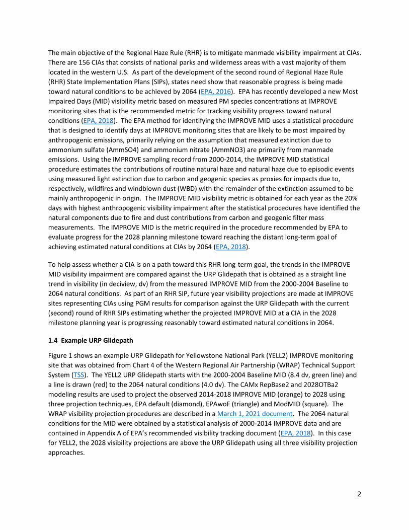
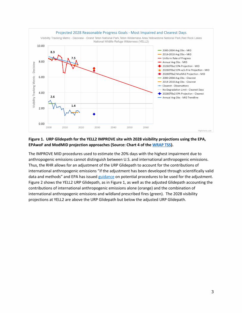
Figure 1 shows an example URP Glidepath for Yellowstone National Park (YELL2) IMPROVE monitoring
site that was obtained from Chart 4 of the Western Regional Air Partnership (WRAP) Technical Support
System (TSS). The YELL2 URP Glidepath starts with the 2000-2004 Baseline MID (8.4 dv, green line) and
a line is drawn (red) to the 2064 natural conditions (4.0 dv). The CAMx RepBase2 and 2028OTBa2
modeling results are used to project the observed 2014-2018 IMPROVE MID (orange) to 2028 using
three projection techniques, EPA default (diamond), EPAwoF (triangle) and ModMID (square). The
WRAP visibility projection procedures are described in a March 1, 2021 document. The 2064 natural
conditions for the MID were obtained by a statistical analysis of 2000-2014 IMPROVE data and are
contained in Appendix A of EPA’s recommended visibility tracking document (EPA, 2018). In this case
for YELL2, the 2028 visibility projections are above the URP Glidepath using all three visibility projection
approaches.
3
Figure 1. URP Glidepath for the YELL2 IMPROVE site with 2028 visibility projections using the EPA,
EPAwoF and ModMID projection approaches (Source: Chart 4 of the WRAP TSS).
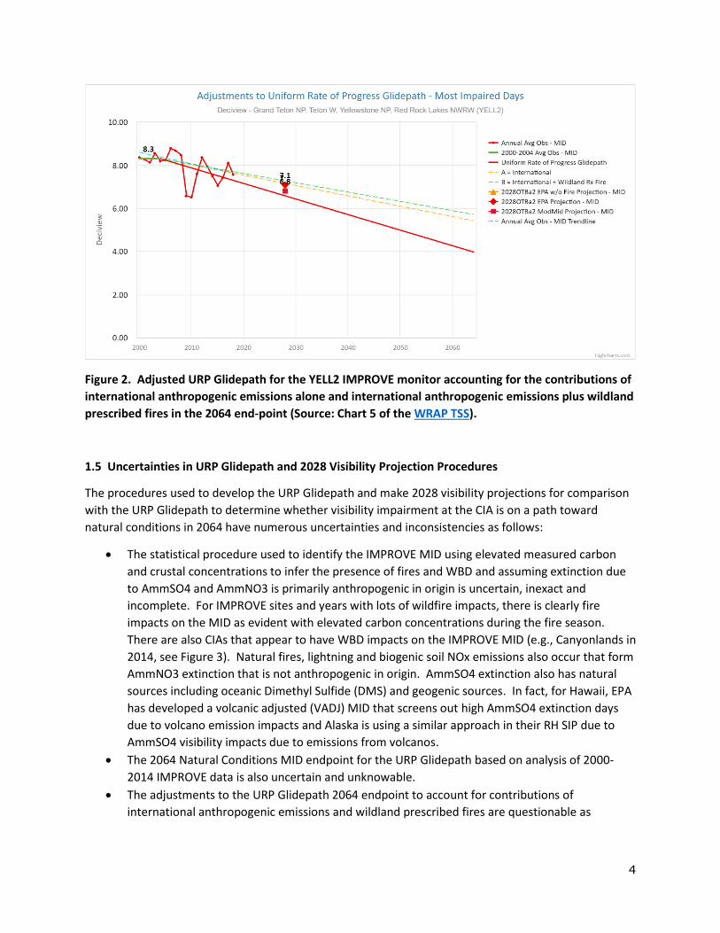
The IMPROVE MID procedures used to estimate the 20% days with the highest impairment due to
anthropogenic emissions cannot distinguish between U.S. and international anthropogenic emissions.
Thus, the RHR allows for an adjustment of the URP Glidepath to account for the contributions of
international anthropogenic emissions “if the adjustment has been developed through scientifically valid
data and methods” and EPA has issued guidance on potential procedures to be used for the adjustment.
Figure 2 shows the YELL2 URP Glidepath, as in Figure 1, as well as the adjusted Glidepath accounting the
contributions of international anthropogenic emissions alone (orange) and the combination of
international anthropogenic emissions and wildland prescribed fires (green). The 2028 visibility
projections at YELL2 are above the URP Glidepath but below the adjusted URP Glidepath.
4
Figure 2. Adjusted URP Glidepath for the YELL2 IMPROVE monitor accounting for the contributions of
international anthropogenic emissions alone and international anthropogenic emissions plus wildland
prescribed fires in the 2064 end-point (Source: Chart 5 of the WRAP TSS).
1.5 Uncertainties in URP Glidepath and 2028 Visibility Projection Procedures
The procedures used to develop the URP Glidepath and make 2028 visibility projections for comparison
with the URP Glidepath to determine whether visibility impairment at the CIA is on a path toward
natural conditions in 2064 have numerous uncertainties and inconsistencies as follows:
• The statistical procedure used to identify the IMPROVE MID using elevated measured carbon
and crustal concentrations to infer the presence of fires and WBD and assuming extinction due
to AmmSO4 and AmmNO3 is primarily anthropogenic in origin is uncertain, inexact and
incomplete. For IMPROVE sites and years with lots of wildfire impacts, there is clearly fire
impacts on the MID as evident with elevated carbon concentrations during the fire season.
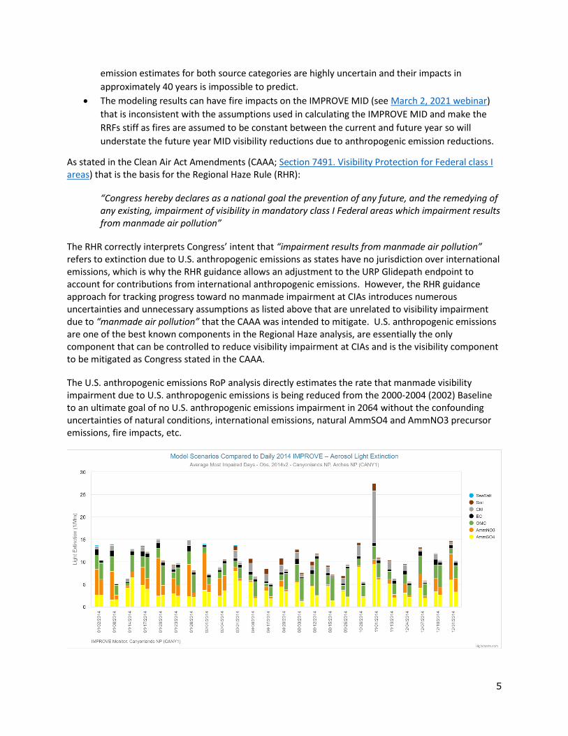
There are also CIAs that appear to have WBD impacts on the IMPROVE MID (e.g., Canyonlands in
2014, see Figure 3). Natural fires, lightning and biogenic soil NOx emissions also occur that form
AmmNO3 extinction that is not anthropogenic in origin. AmmSO4 extinction also has natural
sources including oceanic Dimethyl Sulfide (DMS) and geogenic sources. In fact, for Hawaii, EPA
has developed a volcanic adjusted (VADJ) MID that screens out high AmmSO4 extinction days
due to volcano emission impacts and Alaska is using a similar approach in their RH SIP due to
AmmSO4 visibility impacts due to emissions from volcanos.
• The 2064 Natural Conditions MID endpoint for the URP Glidepath based on analysis of 2000-
2014 IMPROVE data is also uncertain and unknowable.
• The adjustments to the URP Glidepath 2064 endpoint to account for contributions of
international anthropogenic emissions and wildland prescribed fires are questionable as
5
emission estimates for both source categories are highly uncertain and their impacts in
approximately 40 years is impossible to predict.
• The modeling results can have fire impacts on the IMPROVE MID (see March 2, 2021 webinar)
that is inconsistent with the assumptions used in calculating the IMPROVE MID and make the
RRFs stiff as fires are assumed to be constant between the current and future year so will
understate the future year MID visibility reductions due to anthropogenic emission reductions.
As stated in the Clean Air Act Amendments (CAAA; Section 7491. Visibility Protection for Federal class I areas) that is the basis for the Regional Haze Rule (RHR):
“Congress hereby declares as a national goal the prevention of any future, and the remedying of any existing, impairment of visibility in mandatory class I Federal areas which impairment results from manmade air pollution”
The RHR correctly interprets Congress’ intent that “impairment results from manmade air pollution” refers to extinction due to U.S. anthropogenic emissions as states have no jurisdiction over international emissions, which is why the RHR guidance allows an adjustment to the URP Glidepath endpoint to account for contributions from international anthropogenic emissions. However, the RHR guidance approach for tracking progress toward no manmade impairment at CIAs introduces numerous uncertainties and unnecessary assumptions as listed above that are unrelated to visibility impairment due to “manmade air pollution” that the CAAA was intended to mitigate. U.S. anthropogenic emissions are one of the best known components in the Regional Haze analysis, are essentially the only component that can be controlled to reduce visibility impairment at CIAs and is the visibility component to be mitigated as Congress stated in the CAAA.
The U.S. anthropogenic emissions RoP analysis directly estimates the rate that manmade visibility impairment due to U.S. anthropogenic emissions is being reduced from the 2000-2004 (2002) Baseline to an ultimate goal of no U.S. anthropogenic emissions impairment in 2064 without the confounding uncertainties of natural conditions, international emissions, natural AmmSO4 and AmmNO3 precursor emissions, fire impacts, etc.
6
Figure 3. Observed and modeled 2014v2 light extinction at Canyonlands on the 2014 IMPROVE MID showing likely observed WBD impacts on November 1, 2014 (Source WRAP TSS Chart 2).
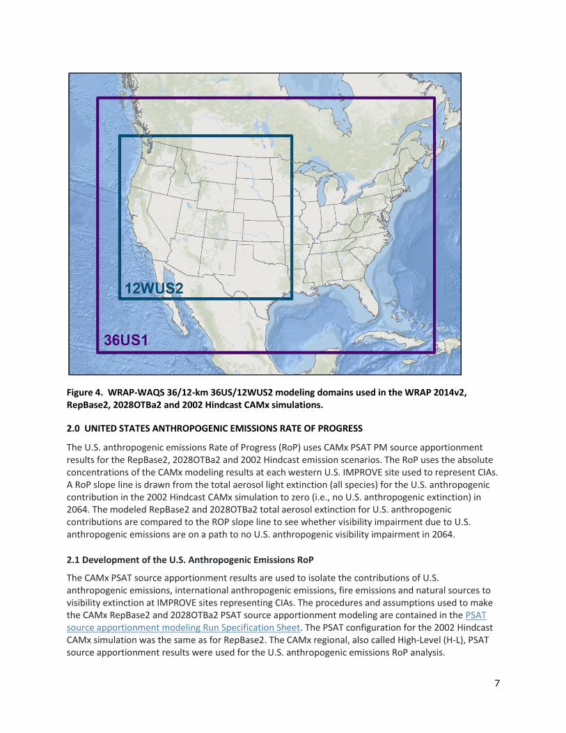
1.6 WRAP Regional Haze Modeling
The Western Regional Air Partnership (WRAP) is conducting PGM modeling for the western states that
includes making 2028 visibility projections at western CIAs for comparison with URP Glidepath to
evaluate whether progress is being made toward natural conditions in 2064. WRAP is using the
Comprehensive Air-quality Model with extension (CAMx) to model the 2014 calendar year using a
36/12-km resolution two-way nested domains (Figure 4) for several emission scenarios, including:
• 2014v2: 2014 actual emissions used in the model performance evaluation (MPE).
• RepBase2: Representative Baseline that represent emissions during the 2014-2018 period,
which are used to project the observed IMPROVE MID from 2014-2018 to the 2028 future year.
• 2028OTBa2: 2028 On-the-Book emissions scenario used in the future year visibility projections.
• 2002 Hindcast: U.S. anthropogenic emissions are backcast to the 2002 year with all other
emissions and boundary conditions held constant at RepBase2 levels.
The assumptions for the RepBase2 and 2028OTBa2 emission scenarios are contained in a
RepBase2/2028OTBa2 Run Specification Sheet. A separate 2002 Dynamic Evaluation Run Specification
Sheet describes the assumptions for the 2002 Hindcast scenario.
EPA’s ozone, PM2.5 and regional haze modeling guidance (EPA, 2018) has recommended procedures for
projecting future year visibility conditions using current and future year modeling results. The EPA-
recommended visibility projection procedure calculates species-specific Relative Response Factors
(RRFs) that are the ratio of future (2028OTBa2) to current (RepBase2) year modeling results averaged
across days in the 2014 IMPROVE MID. The RRFs are used to scale the daily PM species concentrations
from the observed 2014-2018 IMPROVE MID to obtain 2028 future year PM2.5 species concentrations
from which visibility is obtained using the second IMPROVE visibility equation. WRAP has developed
alternative projection methods to the EPA-recommended default approach that differ in how fires are
treated and the days used in the RRFs. The EPA without fire (EPAwoF) visibility projection method is
exactly the same as the EPA default method only contributions from fires are excluded when calculating
the RRFs. A third visibility projection method calculates RRFs using the RepBase2 modeled most
impaired days (ModMID) instead of the 2014 IMPROVE MID and also excludes fire contributions from
the RRF calculations. Details on the three WRAP visibility projection procedures are contained in a
visibility projection document dated March 1, 2021.
7
Figure 4. WRAP-WAQS 36/12-km 36US/12WUS2 modeling domains used in the WRAP 2014v2, RepBase2, 2028OTBa2 and 2002 Hindcast CAMx simulations.
2.0 UNITED STATES ANTHROPOGENIC EMISSIONS RATE OF PROGRESS
The U.S. anthropogenic emissions Rate of Progress (RoP) uses CAMx PSAT PM source apportionment results for the RepBase2, 2028OTBa2 and 2002 Hindcast emission scenarios. The RoP uses the absolute concentrations of the CAMx modeling results at each western U.S. IMPROVE site used to represent CIAs. A RoP slope line is drawn from the total aerosol light extinction (all species) for the U.S. anthropogenic contribution in the 2002 Hindcast CAMx simulation to zero (i.e., no U.S. anthropogenic extinction) in 2064. The modeled RepBase2 and 2028OTBa2 total aerosol extinction for U.S. anthropogenic contributions are compared to the ROP slope line to see whether visibility impairment due to U.S. anthropogenic emissions are on a path to no U.S. anthropogenic visibility impairment in 2064.
2.1 Development of the U.S. Anthropogenic Emissions RoP
The CAMx PSAT source apportionment results are used to isolate the contributions of U.S. anthropogenic emissions, international anthropogenic emissions, fire emissions and natural sources to visibility extinction at IMPROVE sites representing CIAs. The procedures and assumptions used to make the CAMx RepBase2 and 2028OTBa2 PSAT source apportionment modeling are contained in the PSAT source apportionment modeling Run Specification Sheet. The PSAT configuration for the 2002 Hindcast CAMx simulation was the same as for RepBase2. The CAMx regional, also called High-Level (H-L), PSAT source apportionment results were used for the U.S. anthropogenic emissions RoP analysis.
8
The CAMx 2002 Hindcast, RepBase2 and 2028OTBa2 PSAT results were extracted at the western U.S. IMPROVE sites used to represent CIAs for each day of the 2014 calendar year. The revised or second IMPROVE visibility extinction equation (Pitchford et al., 2012) was used to convert the CAMx modeled daily sulfate (SO4), nitrate (NO3), organic aerosol (OA), elemental carbon (EC), elemental PM2.5 species and coarse mass (CM) concentrations into extinction using site-specific relative humidity adjustment factors [f(RH)] with Rayleigh background added to the species extinction to obtain total extinction that can be converted to deciview (dv).
In an approach analogous to the URP Glidepath, a U.S. anthropogenic emissions RoP slope line is obtained by drawing a straight line from the modeled 2002 Hindcast total aerosol light extinction due to U.S. anthropogenic contributions to a 2064 target end-point of no U.S. anthropogenic emissions impairment. The modeled U.S. anthropogenic aerosol extinction from the RepBase2 and 2028OTBa2 results at the CIA are compared to the U.S. anthropogenic emissions RoP slope line to see whether the reduction in extinction from U.S. anthropogenic emissions is on a path toward no U.S. manmade contributions in 2064 (on or below the RoP slope line) or not (above the RoP slope line). Unlike the URP Glideslope that is constructed for the IMPROVE MID from the base year, the RoP slope can be constructed for any set of days from the 2014 modeling year and has been implemented for the 2014 IMPROVE MID, modeled Most Impaired Days (ModMID), IMPROVE sampling days and all 365 days in the year. So rather than examining visibility for a small (~6%) set of days per year as in the URP Glidepath using the IMPROVE MID, the RoP slope line analysis can be conducted for any set of days or even all days in a year.
2.2. U.S. Anthropogenic Emissions RoP Results
The WRAP TSS Model Express Tools Charts 6 and 7 display results of the U.S. anthropogenic emissions RoP:
• Chart 6 – Modeled Visibility Progress – Source Categories: Stacked bar charts of total modeled extinction at IMPROVE sites by source category (U.S. anthropogenic international anthropogenic, fires, natural, and Rayleigh) averaged across the user-selected time periods (IMPROVE MID, ModMID, IMPROVE sampling and all days in 2014) for the 2002 Hindcast, RepBase2 and 2028OTBa2 CAMx simulations.
• Chart 7 – Modeled Visibility Progress – U.S. Anthro Extinction Composition: Stacked bar charts of the species extinction contribution to the total extinction due to U.S. anthropogenic emissions averaged over the user-selected days.
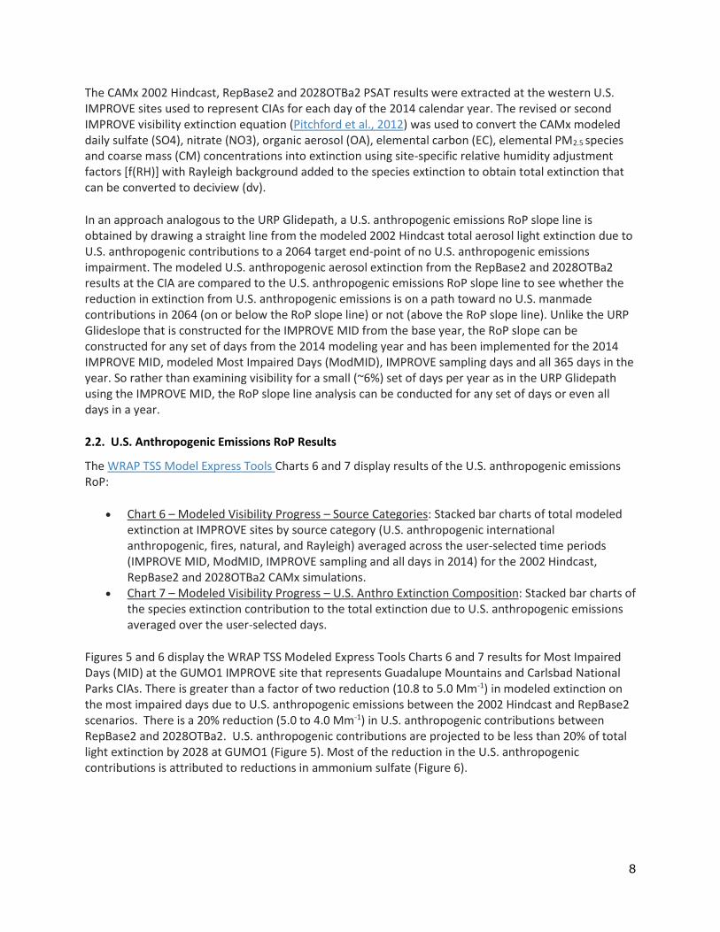
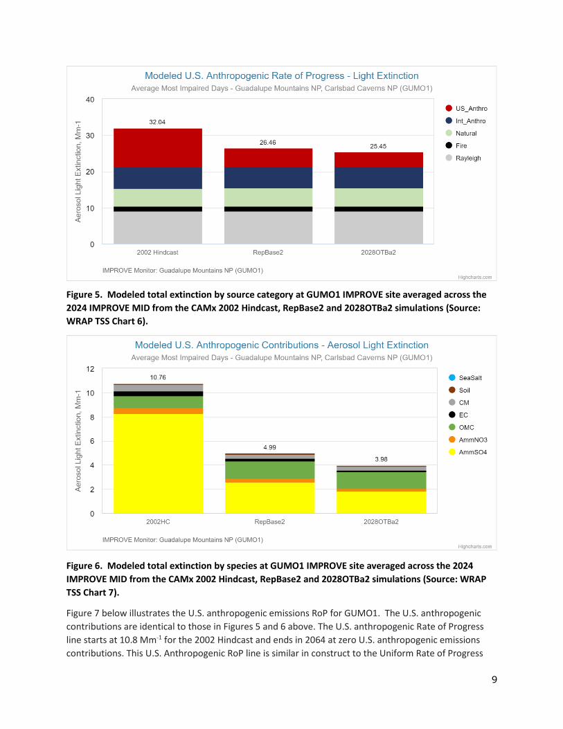
Figures 5 and 6 display the WRAP TSS Modeled Express Tools Charts 6 and 7 results for Most Impaired Days (MID) at the GUMO1 IMPROVE site that represents Guadalupe Mountains and Carlsbad National Parks CIAs. There is greater than a factor of two reduction (10.8 to 5.0 Mm-1) in modeled extinction on the most impaired days due to U.S. anthropogenic emissions between the 2002 Hindcast and RepBase2 scenarios. There is a 20% reduction (5.0 to 4.0 Mm-1) in U.S. anthropogenic contributions between RepBase2 and 2028OTBa2. U.S. anthropogenic contributions are projected to be less than 20% of total light extinction by 2028 at GUMO1 (Figure 5). Most of the reduction in the U.S. anthropogenic contributions is attributed to reductions in ammonium sulfate (Figure 6).
9
Figure 5. Modeled total extinction by source category at GUMO1 IMPROVE site averaged across the
2024 IMPROVE MID from the CAMx 2002 Hindcast, RepBase2 and 2028OTBa2 simulations (Source:
WRAP TSS Chart 6).
Figure 6. Modeled total extinction by species at GUMO1 IMPROVE site averaged across the 2024
IMPROVE MID from the CAMx 2002 Hindcast, RepBase2 and 2028OTBa2 simulations (Source: WRAP
TSS Chart 7).
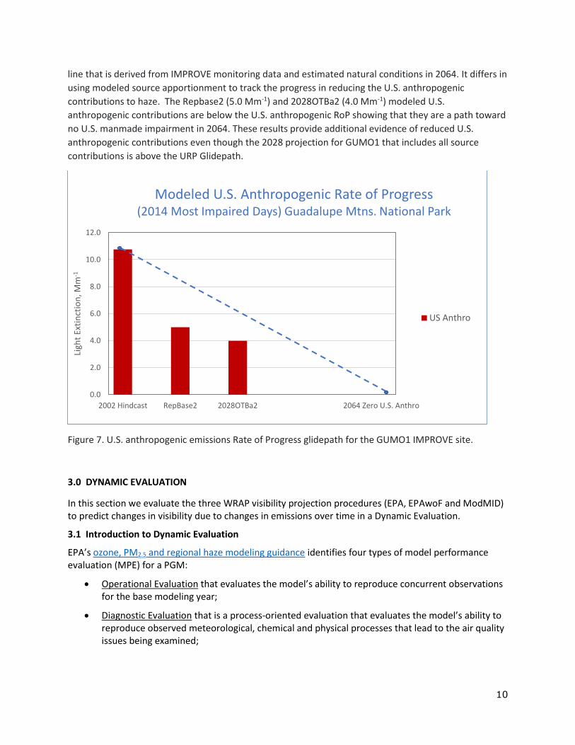
Figure 7 below illustrates the U.S. anthropogenic emissions RoP for GUMO1. The U.S. anthropogenic
contributions are identical to those in Figures 5 and 6 above. The U.S. anthropogenic Rate of Progress
line starts at 10.8 Mm-1 for the 2002 Hindcast and ends in 2064 at zero U.S. anthropogenic emissions
contributions. This U.S. Anthropogenic RoP line is similar in construct to the Uniform Rate of Progress
10
line that is derived from IMPROVE monitoring data and estimated natural conditions in 2064. It differs in
using modeled source apportionment to track the progress in reducing the U.S. anthropogenic
contributions to haze. The Repbase2 (5.0 Mm-1) and 2028OTBa2 (4.0 Mm-1) modeled U.S.
anthropogenic contributions are below the U.S. anthropogenic RoP showing that they are a path toward
no U.S. manmade impairment in 2064. These results provide additional evidence of reduced U.S.
anthropogenic contributions even though the 2028 projection for GUMO1 that includes all source
contributions is above the URP Glidepath.
Figure 7. U.S. anthropogenic emissions Rate of Progress glidepath for the GUMO1 IMPROVE site.
3.0 DYNAMIC EVALUATION
In this section we evaluate the three WRAP visibility projection procedures (EPA, EPAwoF and ModMID) to predict changes in visibility due to changes in emissions over time in a Dynamic Evaluation.
3.1 Introduction to Dynamic Evaluation
EPA’s ozone, PM2.5 and regional haze modeling guidance identifies four types of model performance evaluation (MPE) for a PGM:
• Operational Evaluation that evaluates the model’s ability to reproduce concurrent observations for the base modeling year;
• Diagnostic Evaluation that is a process-oriented evaluation that evaluates the model’s ability to reproduce observed meteorological, chemical and physical processes that lead to the air quality issues being examined;
0.0
2.0
4.0
6.0
8.0
10.0
12.0
2002 Hindcast RepBase2 2028OTBa2 2064 Zero U.S. Anthro
Ligh
t Ex
tin
ctio
n, M
m-1
Modeled U.S. Anthropogenic Rate of Progress (2014 Most Impaired Days) Guadalupe Mtns. National Park
US Anthro
11
• Dynamic Evaluation that evaluates the model’s ability to correctly simulate the changes in concentrations/visibility in response to changes in emissions; and
• Probabilistic Evaluation that assesses the level of confidence in the model predictions through techniques such as ensemble model simulations.
The WRAP regional haze modeling has conducted Operational and Diagnostic Evaluation of the PGM 2014 base case simulations that are available on the WRAP-WAQS 2014 platform development 2014v1 and 2014v2 webpages. The WRAP regional haze Dynamic Evaluation is described below, WRAP did not conduct a Probabilistic Evaluation.
The first step of the Dynamic Evaluation is to backcast the 2014v2 U.S. anthropogenic emissions to the year 2002 so that a CAMx 2002 Hindcast simulation can be conducted. The CAMx 2002 Hindcast simulation uses 2014 meteorological inputs, 2002 U.S. anthropogenic emissions, and the same natural and international emissions and 2014 Boundary Conditions (BCs) as used in the RepBase2 simulation. The procedures used and results for backcasting the 2014v2 U.S. anthropogenic emissions to 2002 are provided in Section 4.0 of this Webpage.
3.2 Dynamic Evaluation Procedures
The same procedures used in the EPA, EPAwoF and ModMID projection methods to project the observed 2014-2018 IMPROVE MID to the 2028 future year using the CAMx RepBase2 and 2028OTBa2 modeling results are used to examine the changes in modeled and observed MID between the current (RepBase2) and past (2002) years. The 2028 visibility projection procedures use EPA’s Software for Modeled Attainment Test (SMAT) tool to project the observed 2014-2018 IMPROVE MID to 2028 using relative response factors (RRFs) that are the ratio of the 2028OTBa2 to RepBase2 modeling results (RRF = 2028OTBa2/RepBase2). The RRFs are used to scale the observed 2014-2018 IMPROVE MID to make the 2028 MID visibility projections (2028 MID = RRF x 2014-2018 IMPROVE MID). Details on the WRAP EPA, EPAwoF and ModMID 2028 visibility projections procedures are described in the WRAP visibility projection document.
The Dynamic Evaluation conducted a 2002DE backward projection where the observed 2014-2018 IMPROVE MID are projected backward to 2002 using the three projection procedures (RRF = 2002 Hindcast / RepBase2) and the 2002DE visibility MID projections are compared against the average of the observed 2000-2004 IMPROVE MID average to determine which projection procedure can best replicate the observed 2000-2004 MID visibility.
In addition to the backward 2002DE visibility projection, the Dynamic Evaluation also conducted a RepBase2DE forward projection by projecting the observed 2000-2004 IMPROVE MID to RepBase2DE using the 2002 Hindcast and RepBase2 CAMx modeling results (RRF = RepBase2 / 2002 Hindcast). The RepBase2DE visibility MID projection is evaluated by comparing it to the observed 2014-2018 IMPROVE MID.
3.3 Dynamic Evaluation Results
The 2002DE and RepBase2DE projected visibility extinction are compared against the observed 5-year average IMPROVE MID from, respectively, 2000-2004 and 2014-2018, for total extinction (TBext), deciview, and for each species component of extinction (AmmSO4, AmmNO3, OMC, EC, Soil and CM). Scatter plots and performance statistics are contained in a Dynamic Evaluation Excel spreadsheet that can be downloaded with a few examples as follows.
12
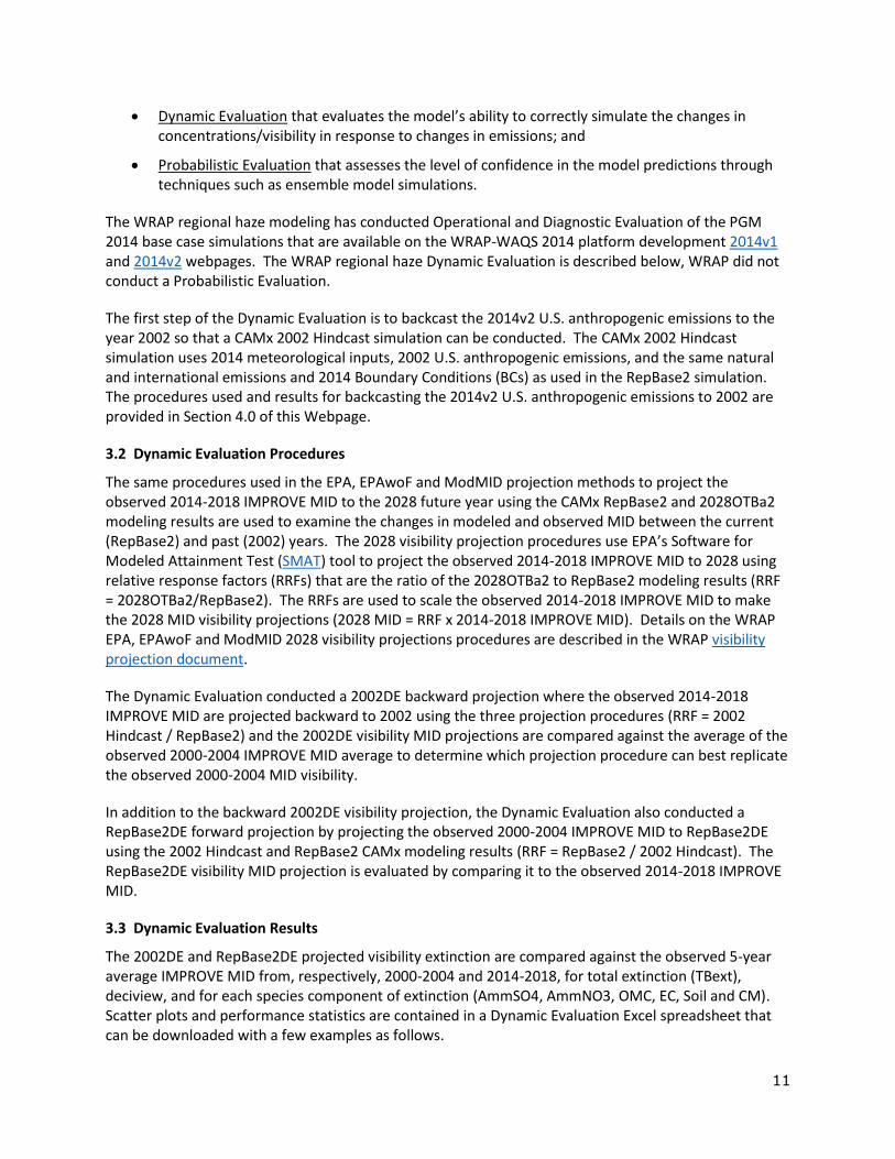
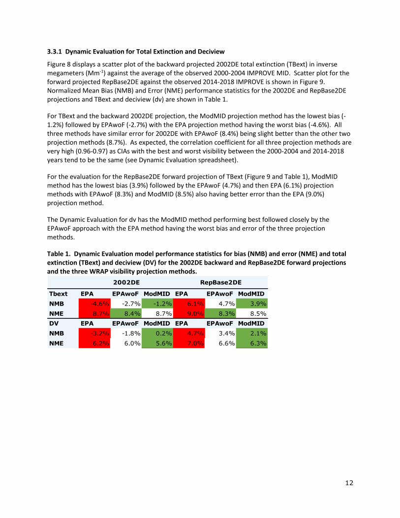
3.3.1 Dynamic Evaluation for Total Extinction and Deciview
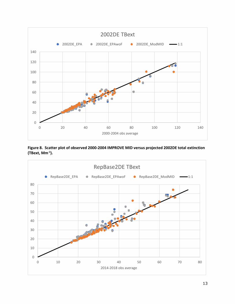
Figure 8 displays a scatter plot of the backward projected 2002DE total extinction (TBext) in inverse megameters (Mm-1) against the average of the observed 2000-2004 IMPROVE MID. Scatter plot for the forward projected RepBase2DE against the observed 2014-2018 IMPROVE is shown in Figure 9. Normalized Mean Bias (NMB) and Error (NME) performance statistics for the 2002DE and RepBase2DE projections and TBext and deciview (dv) are shown in Table 1.
For TBext and the backward 2002DE projection, the ModMID projection method has the lowest bias (-1.2%) followed by EPAwoF (-2.7%) with the EPA projection method having the worst bias (-4.6%). All three methods have similar error for 2002DE with EPAwoF (8.4%) being slight better than the other two projection methods (8.7%). As expected, the correlation coefficient for all three projection methods are very high (0.96-0.97) as CIAs with the best and worst visibility between the 2000-2004 and 2014-2018 years tend to be the same (see Dynamic Evaluation spreadsheet).
For the evaluation for the RepBase2DE forward projection of TBext (Figure 9 and Table 1), ModMID method has the lowest bias (3.9%) followed by the EPAwoF (4.7%) and then EPA (6.1%) projection methods with EPAwoF (8.3%) and ModMID (8.5%) also having better error than the EPA (9.0%) projection method.
The Dynamic Evaluation for dv has the ModMID method performing best followed closely by the EPAwoF approach with the EPA method having the worst bias and error of the three projection methods.
Table 1. Dynamic Evaluation model performance statistics for bias (NMB) and error (NME) and total extinction (TBext) and deciview (DV) for the 2002DE backward and RepBase2DE forward projections and the three WRAP visibility projection methods.
Tbext EPA EPAwoF ModMID EPA EPAwoF ModMID
NMB -4.6% -2.7% -1.2% 6.1% 4.7% 3.9%
NME 8.7% 8.4% 8.7% 9.0% 8.3% 8.5%
2002DE RepBase2DE
DV EPA EPAwoF ModMID EPA EPAwoF ModMID
NMB -3.2% -1.8% 0.2% 4.7% 3.4% 2.1%
NME 6.2% 6.0% 5.6% 7.0% 6.6% 6.3%
13
Figure 8. Scatter plot of observed 2000-2004 IMPROVE MID versus projected 2002DE total extinction (TBext, Mm-1).
0
20
40
60
80
100
120
140
0 20 40 60 80 100 120 140
2000-2004 obs average
2002DE TBext
2002DE_EPA 2002DE_EPAwoF 2002DE_ModMID 1:1
0
10
20
30
40
50
60
70
80
0 10 20 30 40 50 60 70 80
2014-2018 obs average
RepBase2DE TBext
RepBase2DE_EPA RepBase2DE_EPAwoF RepBase2DE_ModMID 1:1
14
Figure 9. Scatter plot of observed 2014-2018 IMPROVE MID versus projected RepBase2DE total extinction (TBext, Mm-1).
3.3.2 Dynamic Evaluation for PM Species Extinction
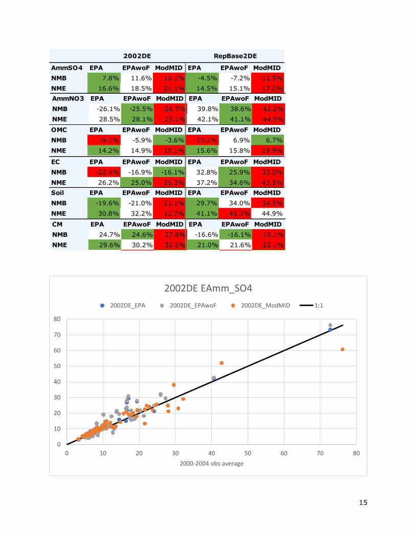
The Dynamic Evaluation for individual extinction components is performed for AmmSO4, AmmNO3 organic mass carbon (OMC), elemental carbon (EC, also called Light Absorbing Carbon, LAC), Soil and coarse mass (CM). Table 2 displays the bias and error performance statistics for the PM extinction components with scatter plots for AmmSO4 and AmmNO3 shown in Figures 10 through 13. Scatter plots for the other species are contained in the Dynamic Evaluation Excel spreadsheet cited earlier.
The EPA projection method performs best for AmmSO4 with the lowest bias for both the 2002DE backward (7.8%) and RepBase2DE forward (-4.5%) projections. The EPAwoF is the next best projection method for AmmSO4 with ModMID being the worst.
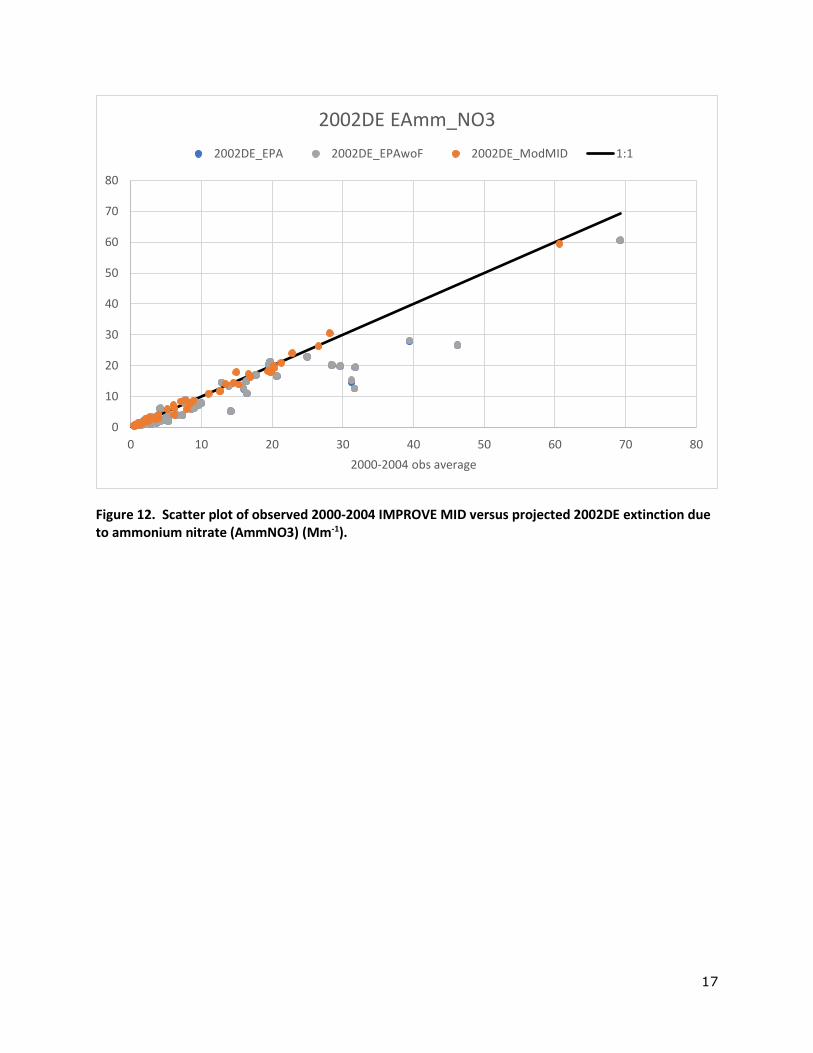
All three projection methods perform poorly for AmmNO3 with a large underestimation bias for the 2002DE backward projection (-26%) and large overestimation bias (39-42%) for the RepBase2DE forward projection. The error is almost the same magnitude as the bias indicating that the underestimation for 2002DE and overestimation for RepBase2DE is almost systematic. Many of the AmmNO3 extinctions are extremely small (Figures 12 and 13) so that small changes in AmmNO3 can produce large percentage changes in the bias and error statistics.
The projection performance for OMC extinction is fairly good with lower bias and error for all three projection methods. The performance statistics are mixed with ModMID having the lowest bias and highest error and EPA having the lowest error but highest bias resulting in EPAwoF being the best performing projection method for OMC. EC extinction has higher bias and error than OMC with EPAwoF being the best performing projection method.
The error and bias values are also higher for Soil and CM with the performance of the EPA and EPAwoF being comparable and the ModMID projection method clearly being the worst performing.
Table 2. Bias (NMB) and error (NME) model performance statistics for the Dynamic Evaluation of the EPA, EPAwoF and ModMID visibility projection methods for the backward (2002DE) and forward (RepBase2DE) projections and the individual light impairing PM species.
15
AmmSO4 EPA EPAwoF ModMID EPA EPAwoF ModMID
NMB 7.8% 11.6% 16.1% -4.5% -7.2% -12.9%
NME 16.6% 18.5% 21.1% 14.5% 15.1% 17.0%
2002DE RepBase2DE
AmmNO3 EPA EPAwoF ModMID EPA EPAwoF ModMID
NMB -26.1% -25.5% -26.7% 39.8% 38.6% 42.2%
NME 28.5% 28.1% 29.1% 42.1% 41.1% 44.9%
OMC EPA EPAwoF ModMID EPA EPAwoF ModMID
NMB -9.1% -5.9% -3.6% 10.2% 6.9% 6.7%
NME 14.2% 14.9% 18.1% 15.6% 15.8% 19.9%
EC EPA EPAwoF ModMID EPA EPAwoF ModMID
NMB -22.4% -16.9% -16.1% 32.8% 25.9% 33.0%
NME 26.2% 25.0% 26.3% 37.2% 34.6% 43.5%
Soil EPA EPAwoF ModMID EPA EPAwoF ModMID
NMB -19.6% -21.0% -21.1% 29.7% 34.0% 34.5%
NME 30.8% 32.2% 32.7% 41.1% 45.3% 44.9%
CM EPA EPAwoF ModMID EPA EPAwoF ModMID
NMB 24.7% 24.6% 27.8% -16.6% -16.1% -18.1%
NME 29.6% 30.2% 32.6% 21.0% 21.6% 22.1%
0
10
20
30
40
50
60
70
80
0 10 20 30 40 50 60 70 80
2000-2004 obs average
2002DE EAmm_SO4
2002DE_EPA 2002DE_EPAwoF 2002DE_ModMID 1:1
16
Figure 10. Scatter plot of observed 2000-2004 IMPROVE MID versus projected 2002DE extinction due to ammonium sulfate (AmmSO4) (Mm-1).
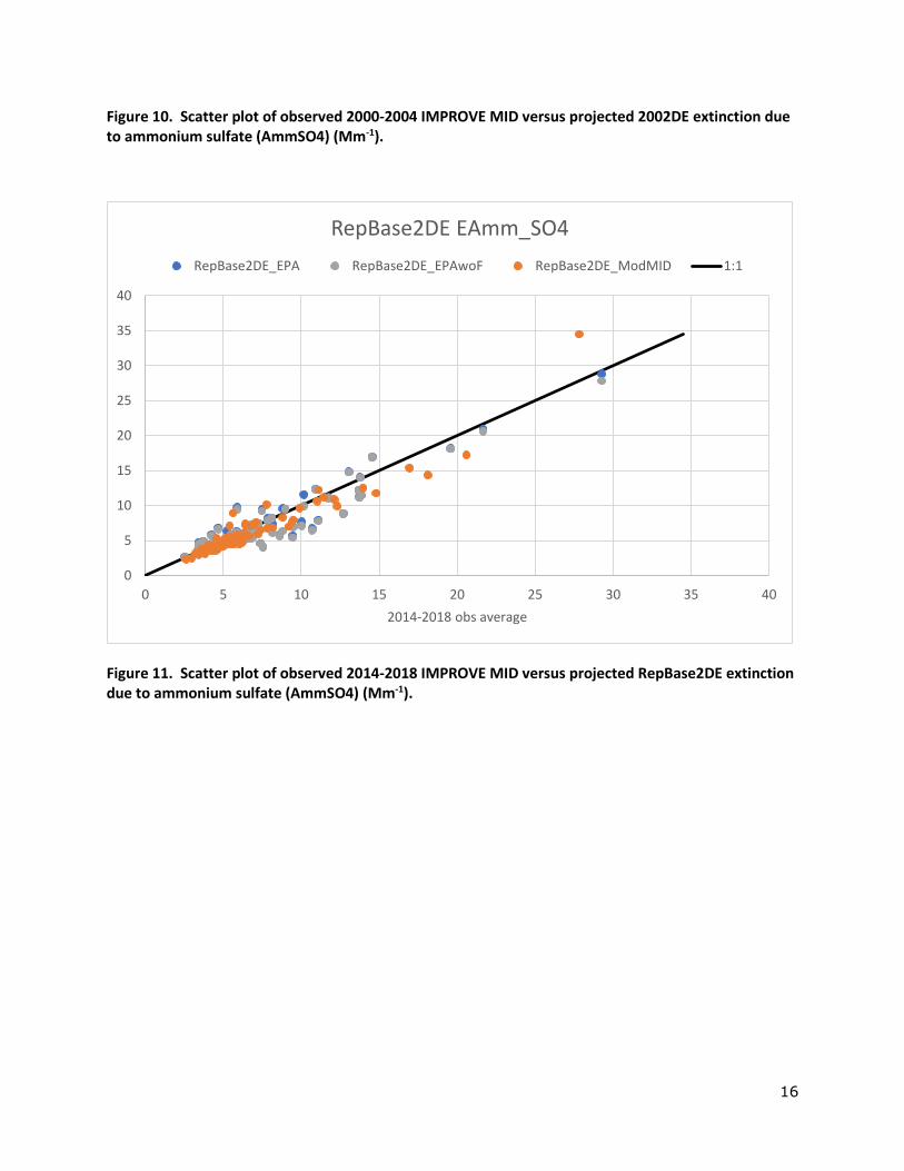
Figure 11. Scatter plot of observed 2014-2018 IMPROVE MID versus projected RepBase2DE extinction due to ammonium sulfate (AmmSO4) (Mm-1).
0
5
10
15
20
25
30
35
40
0 5 10 15 20 25 30 35 40
2014-2018 obs average
RepBase2DE EAmm_SO4
RepBase2DE_EPA RepBase2DE_EPAwoF RepBase2DE_ModMID 1:1
17
Figure 12. Scatter plot of observed 2000-2004 IMPROVE MID versus projected 2002DE extinction due to ammonium nitrate (AmmNO3) (Mm-1).
0
10
20
30
40
50
60
70
80
0 10 20 30 40 50 60 70 80
2000-2004 obs average
2002DE EAmm_NO3
2002DE_EPA 2002DE_EPAwoF 2002DE_ModMID 1:1
18
Figure 13. Scatter plot of observed 2014-2018 IMPROVE MID versus projected RepBase2DE extinction due to ammonium sulfate (AmmSO4) (Mm-1).
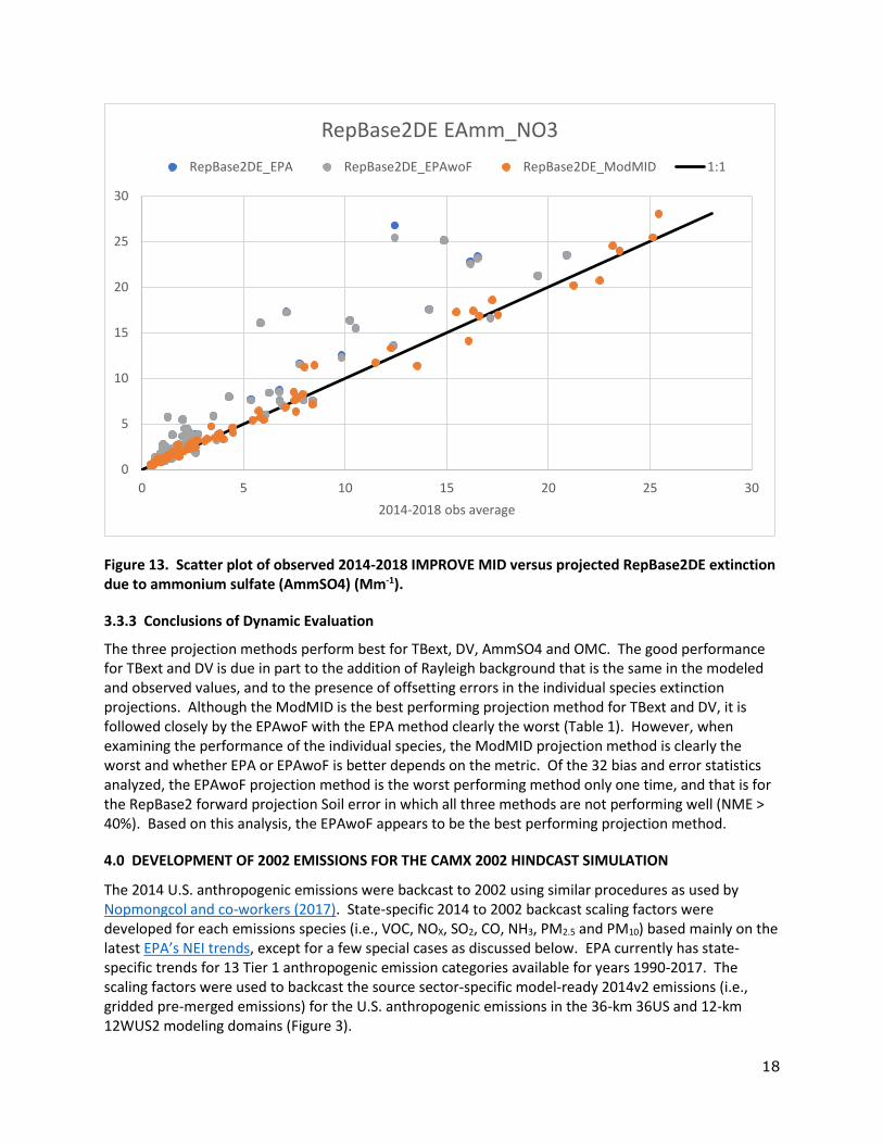
3.3.3 Conclusions of Dynamic Evaluation
The three projection methods perform best for TBext, DV, AmmSO4 and OMC. The good performance for TBext and DV is due in part to the addition of Rayleigh background that is the same in the modeled and observed values, and to the presence of offsetting errors in the individual species extinction projections. Although the ModMID is the best performing projection method for TBext and DV, it is followed closely by the EPAwoF with the EPA method clearly the worst (Table 1). However, when examining the performance of the individual species, the ModMID projection method is clearly the worst and whether EPA or EPAwoF is better depends on the metric. Of the 32 bias and error statistics analyzed, the EPAwoF projection method is the worst performing method only one time, and that is for the RepBase2 forward projection Soil error in which all three methods are not performing well (NME > 40%). Based on this analysis, the EPAwoF appears to be the best performing projection method.
4.0 DEVELOPMENT OF 2002 EMISSIONS FOR THE CAMX 2002 HINDCAST SIMULATION
The 2014 U.S. anthropogenic emissions were backcast to 2002 using similar procedures as used by Nopmongcol and co-workers (2017). State-specific 2014 to 2002 backcast scaling factors were developed for each emissions species (i.e., VOC, NOX, SO2, CO, NH3, PM2.5 and PM10) based mainly on the latest EPA’s NEI trends, except for a few special cases as discussed below. EPA currently has state-specific trends for 13 Tier 1 anthropogenic emission categories available for years 1990-2017. The scaling factors were used to backcast the source sector-specific model-ready 2014v2 emissions (i.e., gridded pre-merged emissions) for the U.S. anthropogenic emissions in the 36-km 36US and 12-km 12WUS2 modeling domains (Figure 3).
0
5
10
15
20
25
30
0 5 10 15 20 25 30
2014-2018 obs average
RepBase2DE EAmm_NO3
RepBase2DE_EPA RepBase2DE_EPAwoF RepBase2DE_ModMID 1:1
19
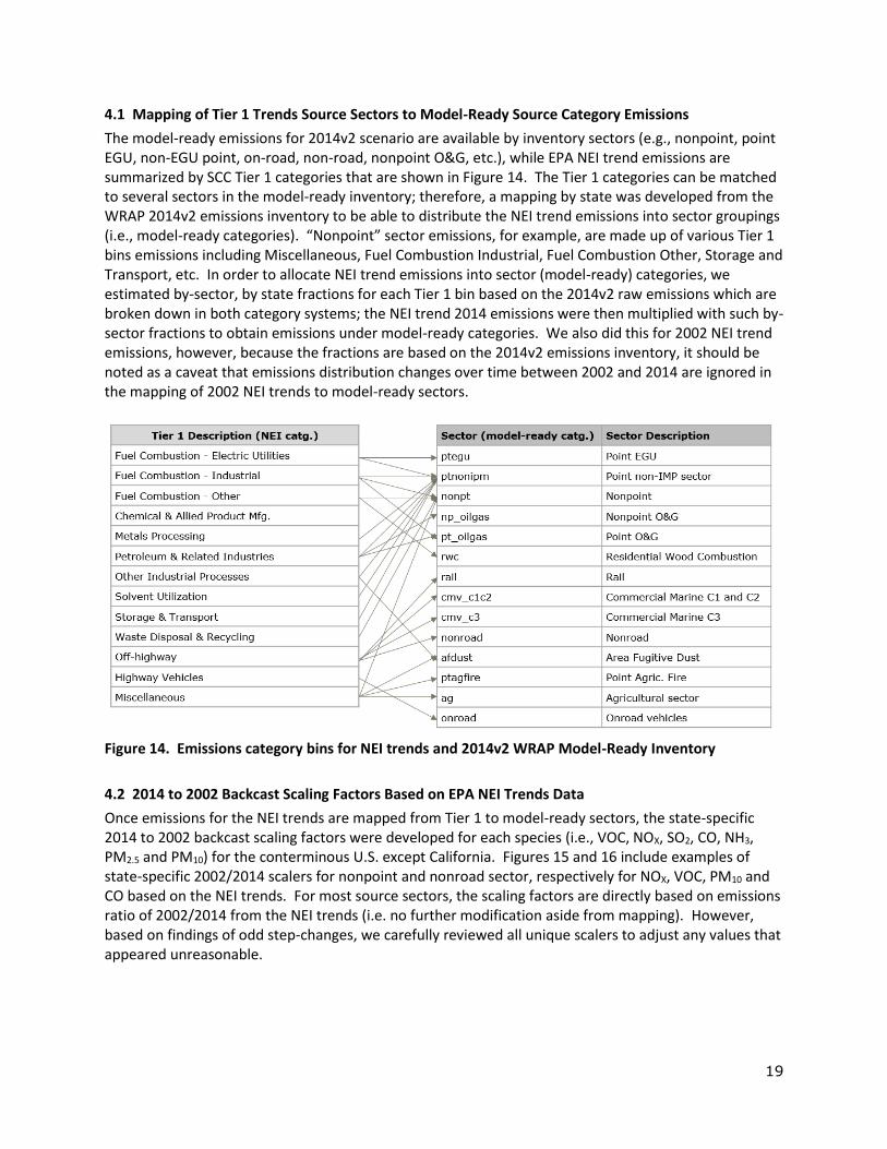
4.1 Mapping of Tier 1 Trends Source Sectors to Model-Ready Source Category Emissions
The model-ready emissions for 2014v2 scenario are available by inventory sectors (e.g., nonpoint, point EGU, non-EGU point, on-road, non-road, nonpoint O&G, etc.), while EPA NEI trend emissions are summarized by SCC Tier 1 categories that are shown in Figure 14. The Tier 1 categories can be matched to several sectors in the model-ready inventory; therefore, a mapping by state was developed from the WRAP 2014v2 emissions inventory to be able to distribute the NEI trend emissions into sector groupings (i.e., model-ready categories). “Nonpoint” sector emissions, for example, are made up of various Tier 1 bins emissions including Miscellaneous, Fuel Combustion Industrial, Fuel Combustion Other, Storage and Transport, etc. In order to allocate NEI trend emissions into sector (model-ready) categories, we estimated by-sector, by state fractions for each Tier 1 bin based on the 2014v2 raw emissions which are broken down in both category systems; the NEI trend 2014 emissions were then multiplied with such by-sector fractions to obtain emissions under model-ready categories. We also did this for 2002 NEI trend emissions, however, because the fractions are based on the 2014v2 emissions inventory, it should be noted as a caveat that emissions distribution changes over time between 2002 and 2014 are ignored in the mapping of 2002 NEI trends to model-ready sectors.
Figure 14. Emissions category bins for NEI trends and 2014v2 WRAP Model-Ready Inventory
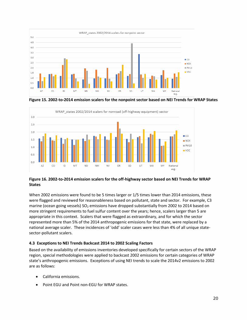
4.2 2014 to 2002 Backcast Scaling Factors Based on EPA NEI Trends Data
Once emissions for the NEI trends are mapped from Tier 1 to model-ready sectors, the state-specific 2014 to 2002 backcast scaling factors were developed for each species (i.e., VOC, NOX, SO2, CO, NH3, PM2.5 and PM10) for the conterminous U.S. except California. Figures 15 and 16 include examples of state-specific 2002/2014 scalers for nonpoint and nonroad sector, respectively for NOX, VOC, PM10 and CO based on the NEI trends. For most source sectors, the scaling factors are directly based on emissions ratio of 2002/2014 from the NEI trends (i.e. no further modification aside from mapping). However, based on findings of odd step-changes, we carefully reviewed all unique scalers to adjust any values that appeared unreasonable.
20
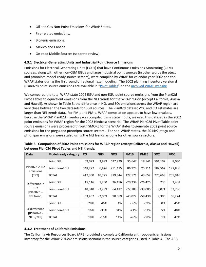
Figure 15. 2002-to-2014 emission scalers for the nonpoint sector based on NEI Trends for WRAP States
Figure 16. 2002-to-2014 emission scalers for the off-highway sector based on NEI Trends for WRAP States
When 2002 emissions were found to be 5 times larger or 1/5 times lower than 2014 emissions, these were flagged and reviewed for reasonableness based on pollutant, state and sector. For example, C3 marine (ocean going vessels) SO2 emissions have dropped substantially from 2002 to 2014 based on more stringent requirements to fuel sulfur content over the years; hence, scalers larger than 5 are appropriate in this context. Scalers that were flagged as extraordinary, and for which the sector represented more than 5% of the 2014 anthropogenic emissions for that state, were replaced by a national average scaler. These incidences of ‘odd’ scaler cases were less than 4% of all unique state-sector-pollutant scalers.
4.3 Exceptions to NEI Trends Backcast 2014 to 2002 Scaling Factors
Based on the availability of emissions inventories developed specifically for certain sectors of the WRAP region, special methodologies were applied to backcast 2002 emissions for certain categories of WRAP state’s anthropogenic emissions. Exceptions of using NEI trends to scale the 2014v2 emissions to 2002 are as follows:
• California emissions.
• Point EGU and Point non-EGU for WRAP states.
21
• Oil and Gas Non-Point Emissions for WRAP States.
• Fire-related emissions.
• Biogenic emissions.
• Mexico and Canada.
• On-road Mobile Sources (separate review).
4.3.1 Electrical Generating Units and Industrial Point Source Emissions
Emissions for Electrical Generating Units (EGUs) that have Continuous Emissions Monitoring (CEM) sources, along with other non-CEM EGUs and large industrial point sources (in other words the ptegu and ptnonipm model-ready source sectors), were compiled by WRAP for calendar year 2002 and the WRAP states during the first round of regional haze modeling. The 2002 planning inventory version d (Plan02d) point source emissions are available in “Pivot Tables” on the archived WRAP website.
We compared the total WRAP state 2002 EGU and non-EGU point source emissions from the Plan02d Pivot Tables to equivalent emissions from the NEI trends for the WRAP region (except California, Alaska and Hawaii). As shown in Table 3, the difference in NOX and SO2 emissions across the WRAP region are very close between the two datasets for EGU sources. The Plan02d dataset VOC and CO estimates are larger than NEI trends data. For PM10 and PM2.5, WRAP compilation appears to have lower values. Because the WRAP Plan02d inventory was compiled using state inputs, we used this dataset as the 2002 point emissions for WRAP region for the 2002 Hindcast scenario. The WRAP Plan02d Pivot Table point source emissions were processed through SMOKE for the WRAP states to generate 2002 point source emissions for the ptegu and ptnonipm source sectors . For non-WRAP states, the 2014v2 ptegu and ptnonipm emissions were scaled using the NEI trends as done for other source sectors.
Table 3. Comparison of 2002 Point emissions for WRAP region (except California, Alaska and Hawaii) between Plan02d Pivot Tables and NEI trends.
Data Model ready category CO NH3 NOX PM10 PM25 SO2 VOC
Plan02d 2002 emissions
(TPY)
Point EGU 69,073 3,899 627,929 35,647 18,541 594,107 8,030
Point non-EGU 348,277 6,826 251,415 86,924 25,111 182,562 197,886
TOTAL 417,350 10,725 879,344 122,571 43,652 776,668 205,916
Difference in TPY
[Plan02d – NEI trend]
Point EGU 15,116 1,230 26,156 -20,234 -26,425 236 2,488
Point non-EGU 48,340 -3,299 64,412 -22,789 -33,005 9,071 63,786
TOTAL 63,457 -2,069 90,569 -43,022 -59,430 9,306 66,274
% difference [(Plan02d - NEI) /NEI]
Point EGU 28% 46% 4% -36% -59% 0% 45%
Point non-EGU 16% -33% 34% -21% -57% 5% 48%
TOTAL 18% -16% 11% -26% -58% 1% 47%
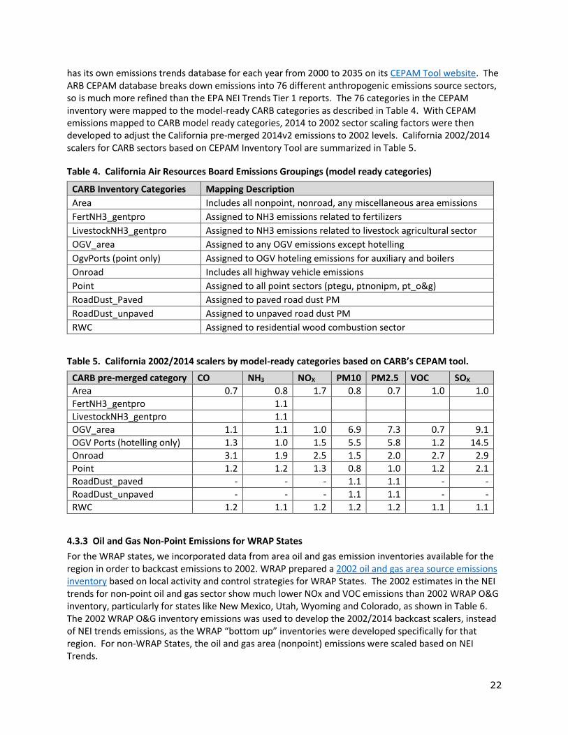
4.3.2 Treatment of California Emissions
The California Air Resources Board (ARB) provided a complete California anthropogenic emissions inventory for the WRAP 2014v2 emissions scenario in the source categories listed in Table 4. The ARB
22
has its own emissions trends database for each year from 2000 to 2035 on its CEPAM Tool website. The ARB CEPAM database breaks down emissions into 76 different anthropogenic emissions source sectors, so is much more refined than the EPA NEI Trends Tier 1 reports. The 76 categories in the CEPAM inventory were mapped to the model-ready CARB categories as described in Table 4. With CEPAM emissions mapped to CARB model ready categories, 2014 to 2002 sector scaling factors were then developed to adjust the California pre-merged 2014v2 emissions to 2002 levels. California 2002/2014 scalers for CARB sectors based on CEPAM Inventory Tool are summarized in Table 5.
Table 4. California Air Resources Board Emissions Groupings (model ready categories)
CARB Inventory Categories Mapping Description
Area Includes all nonpoint, nonroad, any miscellaneous area emissions
FertNH3_gentpro Assigned to NH3 emissions related to fertilizers
LivestockNH3_gentpro Assigned to NH3 emissions related to livestock agricultural sector
OGV_area Assigned to any OGV emissions except hotelling
OgvPorts (point only) Assigned to OGV hoteling emissions for auxiliary and boilers
Onroad Includes all highway vehicle emissions
Point Assigned to all point sectors (ptegu, ptnonipm, pt_o&g)
RoadDust_Paved Assigned to paved road dust PM
RoadDust_unpaved Assigned to unpaved road dust PM
RWC Assigned to residential wood combustion sector
Table 5. California 2002/2014 scalers by model-ready categories based on CARB’s CEPAM tool.
CARB pre-merged category CO NH3 NOX PM10 PM2.5 VOC SOX
Area 0.7 0.8 1.7 0.8 0.7 1.0 1.0
FertNH3_gentpro 1.1 LivestockNH3_gentpro 1.1 OGV_area 1.1 1.1 1.0 6.9 7.3 0.7 9.1
OGV Ports (hotelling only) 1.3 1.0 1.5 5.5 5.8 1.2 14.5
Onroad 3.1 1.9 2.5 1.5 2.0 2.7 2.9
Point 1.2 1.2 1.3 0.8 1.0 1.2 2.1
RoadDust_paved - - - 1.1 1.1 - -
RoadDust_unpaved - - - 1.1 1.1 - -
RWC 1.2 1.1 1.2 1.2 1.2 1.1 1.1
4.3.3 Oil and Gas Non-Point Emissions for WRAP States
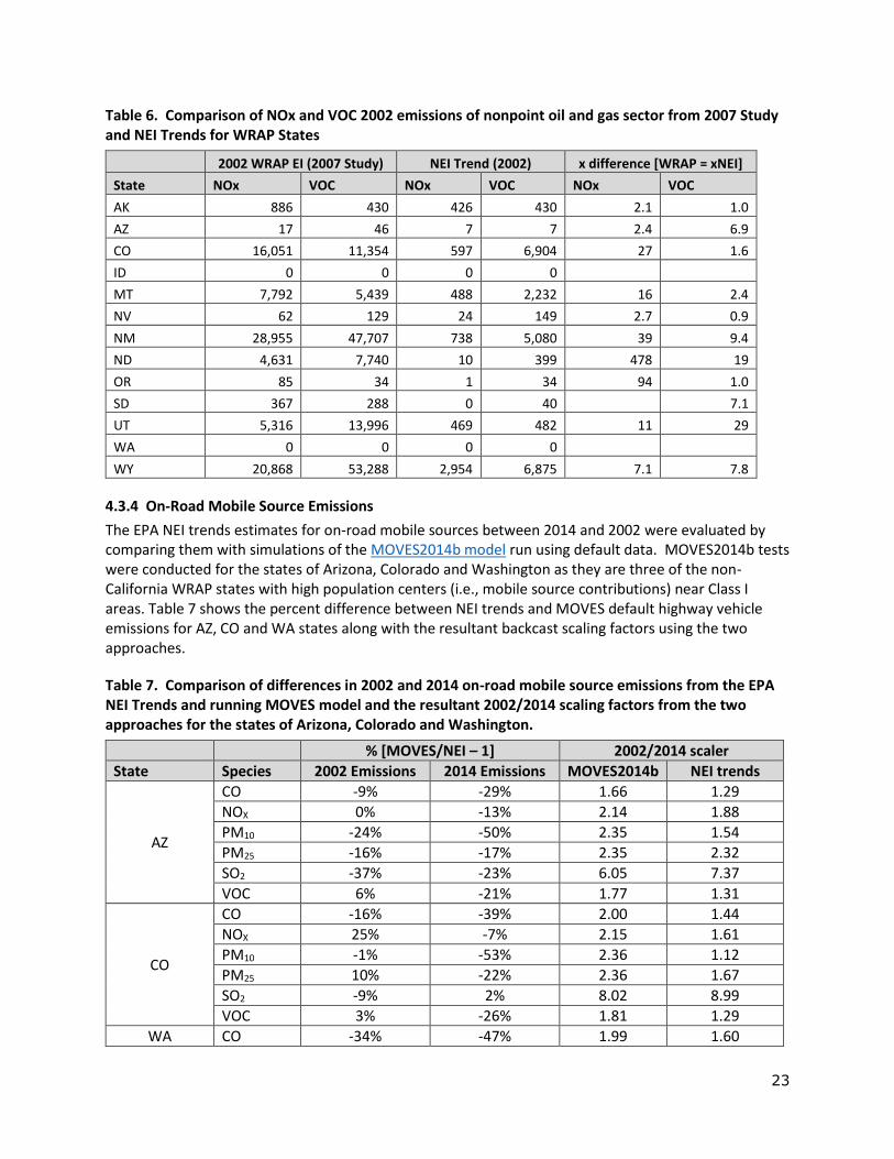
For the WRAP states, we incorporated data from area oil and gas emission inventories available for the region in order to backcast emissions to 2002. WRAP prepared a 2002 oil and gas area source emissions inventory based on local activity and control strategies for WRAP States. The 2002 estimates in the NEI trends for non-point oil and gas sector show much lower NOx and VOC emissions than 2002 WRAP O&G inventory, particularly for states like New Mexico, Utah, Wyoming and Colorado, as shown in Table 6. The 2002 WRAP O&G inventory emissions was used to develop the 2002/2014 backcast scalers, instead of NEI trends emissions, as the WRAP “bottom up” inventories were developed specifically for that region. For non-WRAP States, the oil and gas area (nonpoint) emissions were scaled based on NEI Trends.
23
Table 6. Comparison of NOx and VOC 2002 emissions of nonpoint oil and gas sector from 2007 Study and NEI Trends for WRAP States
2002 WRAP EI (2007 Study) NEI Trend (2002) x difference [WRAP = xNEI]
State NOx VOC NOx VOC NOx VOC
AK 886 430 426 430 2.1 1.0
AZ 17 46 7 7 2.4 6.9
CO 16,051 11,354 597 6,904 27 1.6
ID 0 0 0 0
MT 7,792 5,439 488 2,232 16 2.4
NV 62 129 24 149 2.7 0.9
NM 28,955 47,707 738 5,080 39 9.4
ND 4,631 7,740 10 399 478 19
OR 85 34 1 34 94 1.0
SD 367 288 0 40 7.1
UT 5,316 13,996 469 482 11 29
WA 0 0 0 0
WY 20,868 53,288 2,954 6,875 7.1 7.8
4.3.4 On-Road Mobile Source Emissions
The EPA NEI trends estimates for on-road mobile sources between 2014 and 2002 were evaluated by comparing them with simulations of the MOVES2014b model run using default data. MOVES2014b tests were conducted for the states of Arizona, Colorado and Washington as they are three of the non-California WRAP states with high population centers (i.e., mobile source contributions) near Class I areas. Table 7 shows the percent difference between NEI trends and MOVES default highway vehicle emissions for AZ, CO and WA states along with the resultant backcast scaling factors using the two approaches.
Table 7. Comparison of differences in 2002 and 2014 on-road mobile source emissions from the EPA NEI Trends and running MOVES model and the resultant 2002/2014 scaling factors from the two approaches for the states of Arizona, Colorado and Washington.
% [MOVES/NEI – 1] 2002/2014 scaler
State Species 2002 Emissions 2014 Emissions MOVES2014b NEI trends
AZ
CO -9% -29% 1.66 1.29
NOX 0% -13% 2.14 1.88
PM10 -24% -50% 2.35 1.54
PM25 -16% -17% 2.35 2.32
SO2 -37% -23% 6.05 7.37
VOC 6% -21% 1.77 1.31
CO
CO -16% -39% 2.00 1.44
NOX 25% -7% 2.15 1.61
PM10 -1% -53% 2.36 1.12
PM25 10% -22% 2.36 1.67
SO2 -9% 2% 8.02 8.99
VOC 3% -26% 1.81 1.29
WA CO -34% -47% 1.99 1.60
24
% [MOVES/NEI – 1] 2002/2014 scaler
State Species 2002 Emissions 2014 Emissions MOVES2014b NEI trends
NOX -3% -22% 2.17 1.76
PM10 -20% -56% 2.36 1.30
PM25 -12% -27% 2.36 1.97
SO2 -30% 4% 8.03 11.98
VOC -6% -42% 1.83 1.13
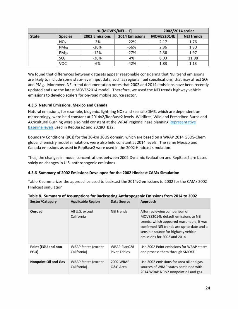
We found that differences between datasets appear reasonable considering that NEI trend emissions are likely to include some state-level input data, such as regional fuel specifications, that may affect SO2 and PM10. Moreover, NEI trend documentation notes that 2002 and 2014 emissions have been recently updated and use the latest MOVES2014 model. Therefore, we used the NEI trends highway vehicle emissions to develop scalers for on-road mobile source sector.
4.3.5 Natural Emissions, Mexico and Canada
Natural emissions, for example, biogenic, lightning NOx and sea salt/DMS, which are dependent on meteorology, were held constant at 2014v2/RepBase2 levels. Wildfires, Wildland Prescribed Burns and Agricultural Burning were also held constant at the WRAP regional haze planning Representative Baseline levels used in RepBase2 and 2028OTBa2.
Boundary Conditions (BCs) for the 36-km 36US domain, which are based on a WRAP 2014 GEOS-Chem global chemistry model simulation, were also held constant at 2014 levels. The same Mexico and Canada emissions as used in RepBase2 were used in the 2002 Hindcast simulation.
Thus, the changes in model concentrations between 2002 Dynamic Evaluation and RepBase2 are based solely on changes in U.S. anthropogenic emissions.
4.3.6 Summary of 2002 Emissions Developed for the 2002 Hindcast CAMx Simulation
Table 8 summarizes the approaches used to backcast the 2014v2 emissions to 2002 for the CAMx 2002
Hindcast simulation.
Table 8. Summary of Assumptions for Backcasting Anthropogenic Emissions from 2014 to 2002
Sector/Category Applicable Region Data Source Approach
Onroad All U.S. except
California
NEI trends After reviewing comparison of
MOVES2014b default emissions to NEI
trends, which appeared reasonable, it was
confirmed NEI trends are up-to-date and a
sensible source for highway vehicle
emissions for 2002 and 2014
Point (EGU and non-
EGU)
WRAP States (except
California)
WRAP Plan02d
Pivot Tables
Use 2002 Point emissions for WRAP states
and process them through SMOKE
Nonpoint Oil and Gas WRAP States (except
California)
2002 WRAP
O&G Area
Use 2002 emissions for area oil and gas
sources of WRAP states combined with
2014 WRAP NEIv2 nonpoint oil and gas
25
Source
Inventory
emissions to develop backcasting scaler
for this sector.
Remaining
anthropogenic
emissions
All U.S. NEI trends Mapped SCC Tier 1 category emissions in
NEI trends to model-ready sectors.
Developed 2002/2014 scalers by state and
by sector
California
Anthropogenic
Emissions
California CARB CEPAM
inventory
Mapped CEPAM emissions to CARB
model-ready categories. Developed
2002/2014 scalers
Natural Emissions and
Agricultural Fires
All U.S. n/a Includes wildfires, biogenics, prescribed
fires, agricultural fires. Assumed to remain
a constant level from Representative
Baseline levels
Mexico and Canada International n/a Assumed to remain a constant level from
2014v2/Representative Baseline
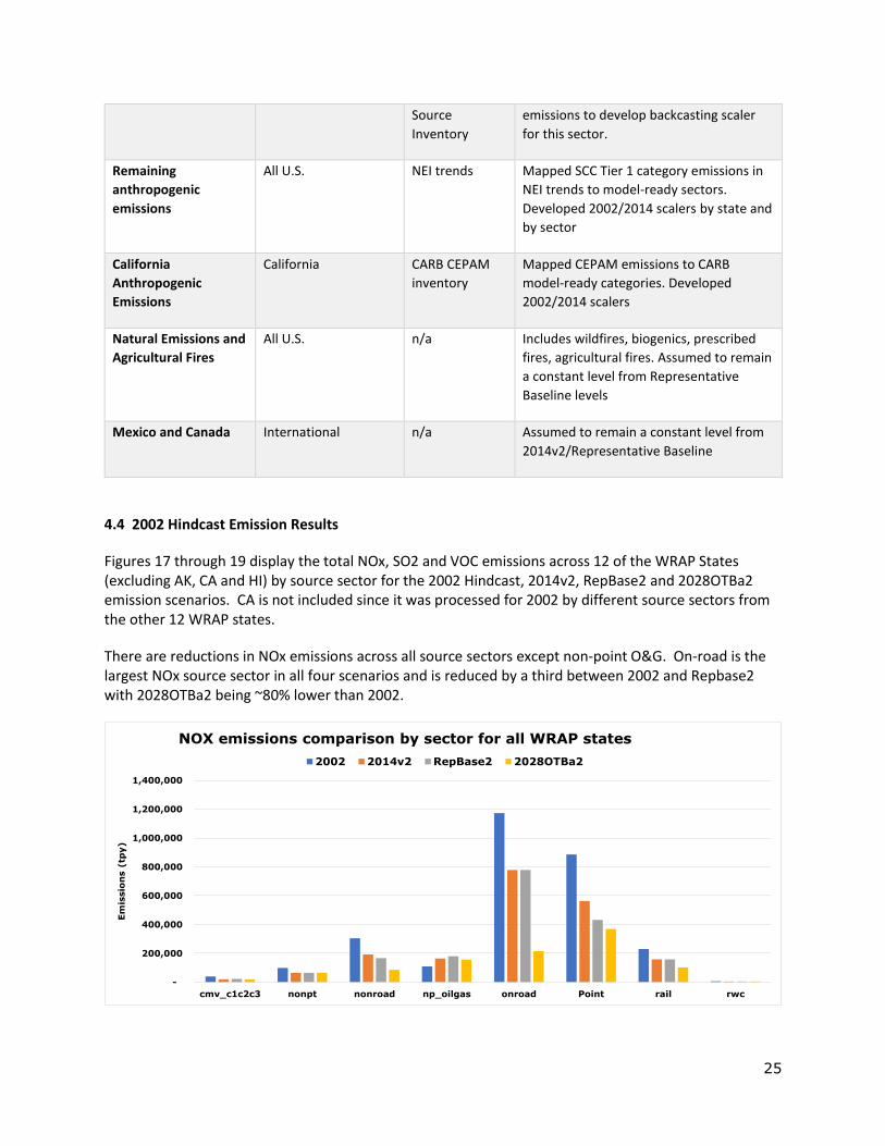
4.4 2002 Hindcast Emission Results
Figures 17 through 19 display the total NOx, SO2 and VOC emissions across 12 of the WRAP States (excluding AK, CA and HI) by source sector for the 2002 Hindcast, 2014v2, RepBase2 and 2028OTBa2 emission scenarios. CA is not included since it was processed for 2002 by different source sectors from the other 12 WRAP states.
There are reductions in NOx emissions across all source sectors except non-point O&G. On-road is the largest NOx source sector in all four scenarios and is reduced by a third between 2002 and Repbase2 with 2028OTBa2 being ~80% lower than 2002.
-
200,000
400,000
600,000
800,000
1,000,000
1,200,000
1,400,000
cmv_c1c2c3 nonpt nonroad np_oilgas onroad Point rail rwc
Em
issio
ns (
tpy)
NOX emissions comparison by sector for all WRAP states
2002 2014v2 RepBase2 2028OTBa2
26
Figure 17. Comparison of source sector NOx emissions across the 13 WRAP states and four emission scenarios.
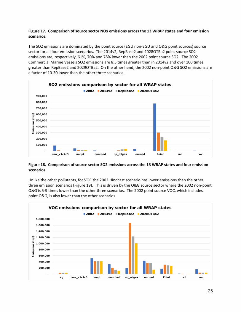
The SO2 emissions are dominated by the point source (EGU non-EGU and O&G point sources) source sector for all four emission scenarios. The 2014v2, RepBase2 and 2028OTBa2 point source SO2 emissions are, respectively, 61%, 70% and 78% lower than the 2002 point source SO2. The 2002 Commercial Marine Vessels SO2 emissions are 8.5 times greater than in 2014v2 and over 100 times greater than RepBase2 and 2029OTBa2. On the other hand, the 2002 non-point O&G SO2 emissions are a factor of 10-30 lower than the other three scenarios.
Figure 18. Comparison of source sector SO2 emissions across the 13 WRAP states and four emission scenarios.
Unlike the other pollutants, for VOC the 2002 Hindcast scenario has lower emissions than the other three emission scenarios (Figure 19). This is driven by the O&G source sector where the 2002 non-point O&G is 5-9 times lower than the other three scenarios. The 2002 point source VOC, which includes point O&G, is also lower than the other scenarios.
-
100,000
200,000
300,000
400,000
500,000
600,000
700,000
800,000
900,000
cmv_c1c2c3 nonpt nonroad np_oilgas onroad Point rail rwc
Em
issio
ns (
tpy)
SO2 emissions comparison by sector for all WRAP states
2002 2014v2 RepBase2 2028OTBa2
-
200,000
400,000
600,000
800,000
1,000,000
1,200,000
1,400,000
1,600,000
1,800,000
ag cmv_c1c2c3 nonpt nonroad np_oilgas onroad Point rail rwc
Em
issio
ns (
tpy)
VOC emissions comparison by sector for all WRAP states
2002 2014v2 RepBase2 2028OTBa2
27
Figure 19. Comparison of source sector SO2 emissions across the 13 WRAP states and four emission scenarios.
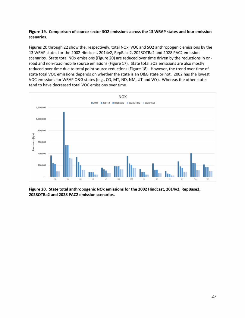
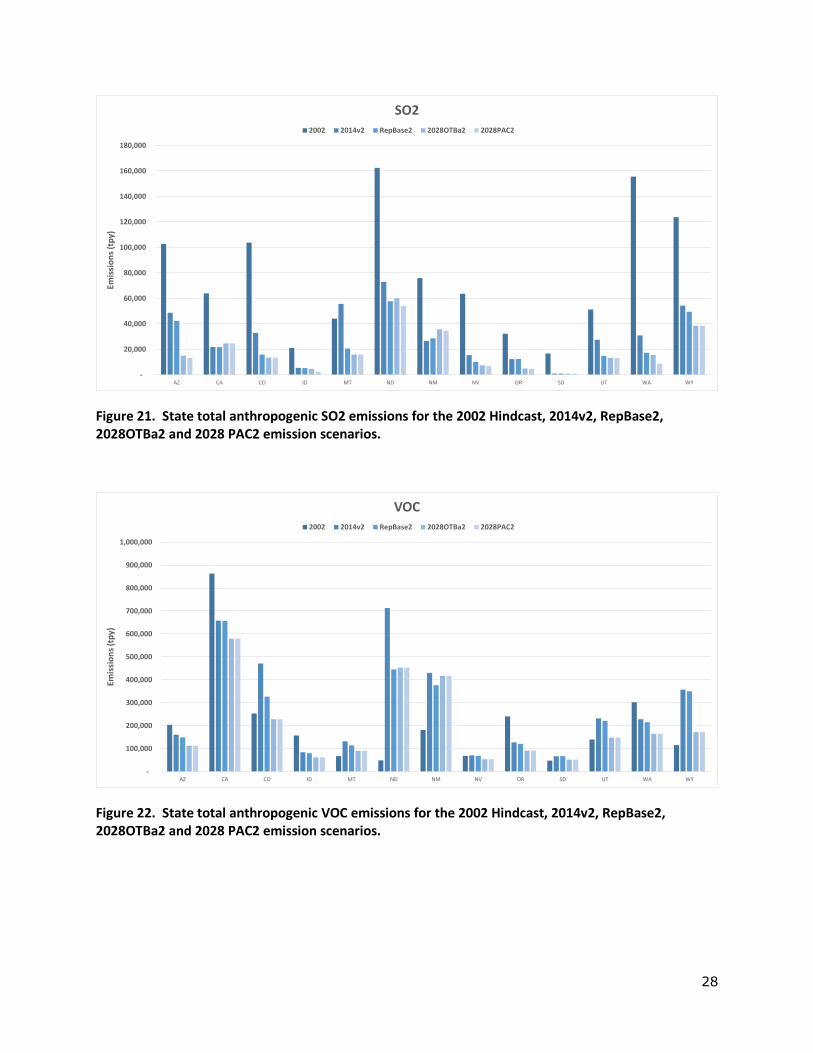
Figures 20 through 22 show the, respectively, total NOx, VOC and SO2 anthropogenic emissions by the 13 WRAP states for the 2002 Hindcast, 2014v2, RepBase2, 2028OTBa2 and 2028 PAC2 emission scenarios. State total NOx emissions (Figure 20) are reduced over time driven by the reductions in on-road and non-road mobile source emissions (Figure 17). State total SO2 emissions are also mostly reduced over time due to total point source reductions (Figure 18). However, the trend over time of state total VOC emissions depends on whether the state is an O&G state or not. 2002 has the lowest VOC emissions for WRAP O&G states (e.g., CO, MT, ND, NM, UT and WY). Whereas the other states tend to have decreased total VOC emissions over time.
Figure 20. State total anthropogenic NOx emissions for the 2002 Hindcast, 2014v2, RepBase2, 2028OTBa2 and 2028 PAC2 emission scenarios.
-
200,000
400,000
600,000
800,000
1,000,000
1,200,000
AZ CA CO ID MT ND NM NV OR SD UT WA WY
Emis
sio
ns
(tp
y)
NOX2002 2014v2 RepBase2 2028OTBa2 2028PAC2
28
Figure 21. State total anthropogenic SO2 emissions for the 2002 Hindcast, 2014v2, RepBase2, 2028OTBa2 and 2028 PAC2 emission scenarios.
Figure 22. State total anthropogenic VOC emissions for the 2002 Hindcast, 2014v2, RepBase2, 2028OTBa2 and 2028 PAC2 emission scenarios.
-
20,000
40,000
60,000
80,000
100,000
120,000
140,000
160,000
180,000
AZ CA CO ID MT ND NM NV OR SD UT WA WY
Emis
sio
ns
(tp
y)SO2
2002 2014v2 RepBase2 2028OTBa2 2028PAC2
-
100,000
200,000
300,000
400,000
500,000
600,000
700,000
800,000
900,000
1,000,000
AZ CA CO ID MT ND NM NV OR SD UT WA WY
Emis
sio
ns
(tp
y)
VOC2002 2014v2 RepBase2 2028OTBa2 2028PAC2