United States Department of the Interior

Translation No. Bureau of Reclamation

Team No. General Engineering and Research Center

Book No. 12,721

• ....... • . ........ • ........... • . •

DESIGNING SPILLWAY AERATORS

Dimensionierung von Scharinnenbeleftern

by

Hans-Peter Koschitzky

Translated from the West German Journal Wasserwirtschaft

5/88, May 1988, 220 - 227

Dr. Sue Ellen Wright, Translator

XXXXXXXXXXXXICXXXXXXXXXXXXXXXXXXXXXXXXXXXXXXXXXXXXXXXXXXXXXXXXXXX=XXXXXXXXX

Division of Foreign Activities

USBR Translations Code D-2000

Denver, Colorado (October, 1988)

Team No. General Book No. 12,721 Paper No.

DESIGNING SPILLWAY AERATORS

Dimensionierung von SchuBrinnenbelliftern

Hans-Peter Koschitzky

Abstract

A design procedure to prevent cavitation damage in spillway aerators is presented and the design steps are explained. The central topic is the design of the bottom aerator. Air entrainment functions required for designing dif-ferent aerator geometries are given based on studies using a hydraulic model and on published data. A calculation method for determining total air en-trainment is presented that considers the interaction between water flow in the spillway and air flow in the aerator. The influence of aeration on high-speed flow is discussed and approaches for calculating this factor are given.

1. Introductory Comment

The kind of high-speed flow occurring in concrete spillways and sluiceways can

rapidly lead to structural damage resulting from cavitation and related cavitation

erosion. Numerous cases of damage confirm this observation [1, 2, 10, 121.

One effective option that has already been used in numerous systems to pre-

vent this kind of damage is the installation of bottom aerators to aerate the flow. For

instance, [5] and [211 provide comprehensive discussions of aerator geometries that

have been utilized for this purpose.

Although there is as yet no clear-cut scientific explanation how the air en-

trained in the water prevents cavitation damage, it has been known for a long time

that even a 5% to 8% air component [13] is adequate to prevent cavitation damage.

Moreover, Russel [15] has demonstrated the effectiveness of air entrainment by con-

ducting studies in a cavitation channel using a velocity of 46 m/s. Within half an

hour exposure, concrete samples exposed to flow without air entrainment suffered

2

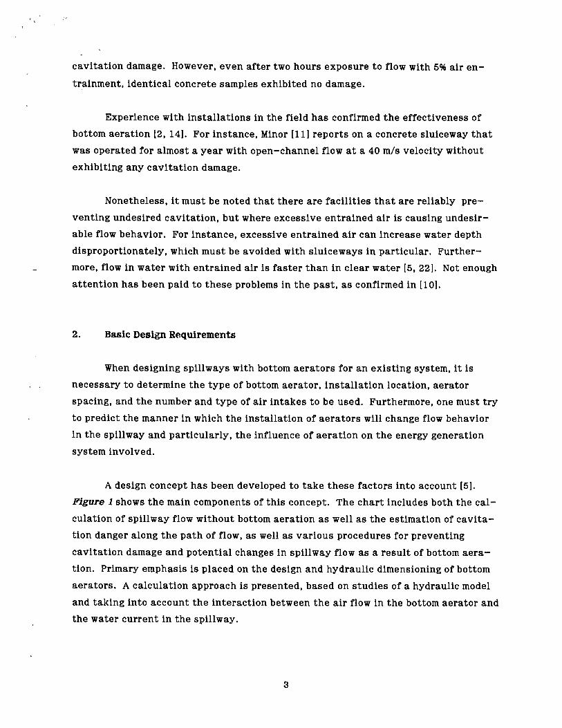
cavitation damage. However, even after two hours exposure to flow with 5% air en—

trainment, identical concrete samples exhibited no damage.

Experience with installations in the field has confirmed the effectiveness of

bottom aeration [2, 14]. For instance, Minor [11] reports on a concrete sluiceway that

was operated for almost a year with open—channel flow at a 40 m/s velocity without

exhibiting any cavitation damage.

Nonetheless, it must be noted that there are facilities that are reliably pre—

venting undesired cavitation, but where excessive entrained air is causing undesir—

able flow behavior. For instance, excessive entrained air can increase water depth

disproportionately, which must be avoided with sluiceways in particular. Further—

more, flow in water with entrained air is faster than in clear water [5, 221. Not enough

attention has been paid to these problems in the past, as confirmed in [10].

2. Basic Design Requirements

When designing spillways with bottom aerators for an existing system, it is

necessary to determine the type of bottom aerator, installation location, aerator

spacing, and the number and type of air intakes to be used. Furthermore, one must try

to predict the manner in which the installation of aerators will change flow behavior

in the spillway and particularly, the influence of aeration on the energy generation

system involved.

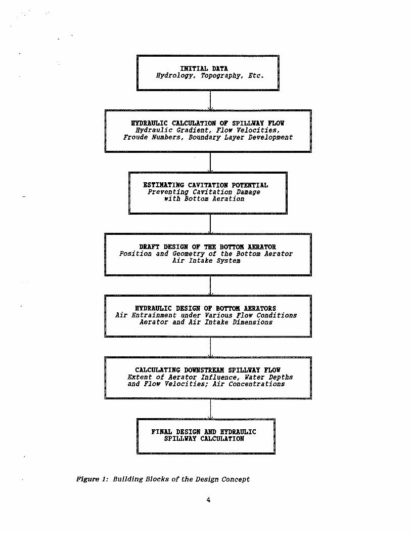
A design concept has been developed to take these factors into account [5].

Figure 1 shows the main components of this concept. The chart includes both the cal—

culation of spillway flow without bottom aeration as well as the estimation of cavita—

tion danger along the path of flow, as well as various procedures for preventing

cavitation damage and potential changes in spillway flow as a result of bottom aera—

tion. Primary emphasis is placed on the design and hydraulic dimensioning of bottom

aerators. A calculation approach is presented, based on studies of a hydraulic model

and taking into account the interaction between the air flow in the bottom aerator and

the water current in the spillway.

3

INITIAL DATA Hydrology, Topography, Etc.

HYDRAULIC CALCULATION OF SPILLWAY FLOW Hydraulic Gradient, Flow Velocities,

Fronde Numbers, Boundary Layer Development

ESTIMATING CAVITATION POTENTIAL Preventing Cavitation Damage

with Bottom Aeration

DRAFT DESIGN OF THE BOTTOM AERATOR Position and Geometry of the Bottom Aerator

Air Intake System

HYDRAULIC DESIGN OF BOTTOM AERATORS Air Entrainment under Various Flow Conditions

Aerator and Air Intake Dimensions

CALCULATING DOWNSTREAM SPILLWAY FLOW Extent of Aerator Influence, Water Depths and Flow Velocities; Air Concentrations

FINAL DESIGN AND HYDRAULIC SPILLWAY CALCULATION

Figure I: Building Blocks of the Design Concept

TOTAL AIR

ATMOSPHERIC

ENTRAINITENT PRESSURE Pa,

AIR INTAKE SYSTEM Nairrd

4I\

TWO-DIPENSIONAL

CROSS SECTION

r BOTTCP1

LOW • PRESSURE Ap SPECIFI AIR

ENTRAINMENT tt P < Patm

WATER

ANTURE

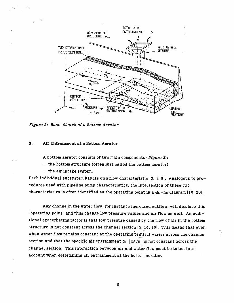
Figure 2: Basic Sketch of a Bottom Aerator

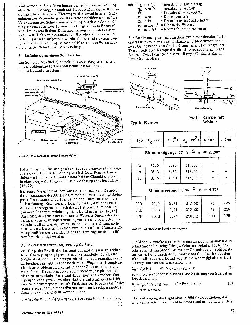
3. Air Entrainment at a Bottom Aerator

A bottom aerator consists of two main components (Figure 2):

- the bottom structure (often just called the bottom aerator)

- the air intake system.

Each individual subsystem has its own flow characteristic [3, 4, 61. Analogous to pro-

cedures used with pipeline pump characteristics, the intersection of these two

characteristics is often identified as the operating point in a QL -Ap diagram [16, 20].

Any change in the water flow, for instance increased outflow, will displace this

"operating point" and thus change low pressure values and air flow as well. An addi-

tional exacerbating factor is that low pressure caused by the flow of air in the bottom

structure is not constant across the channel section [5, 14, 161. This means that even

when water flow remains constant at the operating print, it varies across the channel

section and that the specific air entrainment I m2 Is I is not constant across the

channel section. This interaction between air and water flow must be taken into

account when determining air entrainment at the bottom aerator.

5

t‘

Figure 3.

CROSS SECTIONAL AREA

Type I: Ramp

CROSS Ao SECTIONAL AREA

Type H: Ramp with Bottom Groove

3.1 Two—Dimensional Air Entrainment Function

Although the question of the physics of air entrainment has been considered in

a basic study [3] and conceptual models have been attempted [6, 71, no one has as yet

described the air entrainment mechanism in a precise, formulaic way. Given the com—

plexity of the problem, we are not likely to see this in the near future. Consequently,

we must attempt to develop empirical approaches to the problem. Based on analytical

dimensional considerations, it is possible to demonstrate that the air entrainment rate

for a bottom aerator geometry can be represented as a function of the Froude number

Fr of the water flow and a non—dimensional pressure parameter Ap/Pw`ryw:

(for a given geometry) (1) Where: q. in m2 /s = Specific air entrainment

qw in m2 /s = Specific water outflow

Fr = Froude number = vw/Vg71-4, yw in m = Clear water depth

tip in Pa = Low pressure in the bottom aerator

Pw in kg/m3 = Water density

g in m/s2 = Normal case acceleration

Vif in m/s = Clear water velocity

In order to determine the two—dimensional air entrainment function, extensive

tests were conducted using a model with two basic types of bottom aerators (Figure 3).

Type 1 represents a ramp for use in steep channels, and Type II incorporates a bottom

groove with a ramp for flat channels or sluiceways.

AIR INTAKE AIR

INTAKE

6

Typ tR (mm) e (°) A0 (cm2) s (mm) t (mm)

CHANNEL SLOPE : 37 % '2: m == 20.300

IA 25.0 5,20 215,00 _ _

IB 31,3 6.54 215,00 - -

IC 37.5 7.90 215.00

CHANNEL SLOPE : 3 Vo == m = 1.72°

IID 40.0 5.71 312.50 75 225

IIE 50.0 5.71 312.50 75 225

IIF 50.0 5.71 250.12 100 175

Figure 3, cont. from previous page: Types of Bottom Aerators Studied

The model studies were conducted in a two—dimensional crosssectional model,

which is described in detail in [5, 61. Low pressure values in the bottom aerator were

varied in the model and reduced to a value of zero using a blower. Thus it was possi—

ble to determine the relationship between the air entrainment rate and the water flow

A p (2) 130 = ft, (Fr) (for — 0)

p w * g * yw

as well as the change in S for a given Froude number with the pressure parameter

A P (3) Bp = fp ) (for Fr = constant)

p w * g * yw

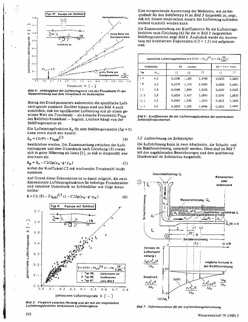
When the results are plotted in Figure 4, it becomes clear that the specific air

entrainment rate increases as the Froude number increases on the one hand and the

value of the pressure parameter decreases on the other hand. Figure 4 also reveals

that significant air entrainment does not begin until the Froude number reaches a

certain value -- identified here as the critical Froude number Fre r t of the

7

Frcr 3,5

ATMOSPHERIC PRESSURE

TYPE IIF: RAMP WITH BOTTOM SLOT

\\ /7

01 a •

0.0 2 0 3.0 4.0 5.0 6:0 7.0 9.0 9.0 10.0 11.0 12.0 13.0 14.0

SP

EC

IFIC

AIR

Q •3

, LOW PRESSURE // PARAMETER • - VALUES

LOW Ap PRESSURE

HIGH PRESSURE Ap

PARAMETER VALUEp;,z:

0.8

' 0.7

C2 0.6

0.5

0.1

3%

Froude Number Fr

Figure 4: Air entrainment rate as a function of the Froude number Fr of the water flow and the low pressure in the bottom aerator

aerator. The latter is a function of aerator geometry. Thus the air entrainment func-

tion Bo can be described for an aerator geometry (tp = 0) with the following formula:

= Cl (Fr - Frtrit)C3 (4)

The relationship between the air entrainment rate and the low pressure value accord-

ing to equation (3) approximates a linear equation [51, so that it can be represented

as:

p = i 0 - C2(Ap/pw • g • yw ) (5)

where the coefficient C2 increases slightly as the Froude number increases.

Based on these findings, it is possible to represent the two-dimensional air

entrainment function for any Froude number and variable low pressure values in the

bottom aerator as follows:

13 =c1 (Fr - Frcrit)C C2Ap/pw • g •_yw (6)

8

0 . 8 0 . 1 0 . 2 0 . 3 0 • 4 0 . 5 0 • 6 0 . 7

xx xx v

ync: X

401Y Y

Ap 8 = Cl(Fr - Frc 1'5 C2 P.gY.

v Typ HD, NUMERICAL VALUES OF THE

z Typ „r """ COEFFICIENTS:

Typ 11F, SEE FIGURE 6

0 . 7

0 . 6

. 5

0 . 4

0 . 3

0 . 2

0. I

0 • 0 00

CZ

CALCULATED AIR ENTRAINMENT RATE

A corresponding evaluation of measured data such as that represented in the

example of a Type II aerator in Figure 5 reveals that this empirical approach is satis-

factory for determining air entrainment.

Figure 6 illustrates the combination of the coefficients for the air entrainment func-

tion according to Equation (6) for the aerator geometries represented in Figure 3.

Evaluation using the constant exponents (C3 = 1.5) was also included in this chart.

3.2 Air Flow in the Bottom Aerator

Air flow can be divided into two components, the shaft and the aerator flow.

Figure 7illustrates the terms and variables used to identify the components of the

system and includes the qualitative pressure curve in the bottom structure.

TYPE II RAIri3 WITH BOTTOM SLOT

MEASURED AIR ENTRAINMENT RATE

Figure 5: Comparison between measured and calculated air entrainment rate based on the empirical air entrainment function

9

WATER FLOW Q.,

1.0 z/B

i i+1 ;+2 II I

Az

AERATOR FLOW

0,5

CHANNEL AXIS OR

SIDEWALL

POTENTIAL AIR FLOW

LOSS AN, 05-

BACK-UP PRESSURE

cio+iiSPECIFIC_AIR ENTRAINMENT OL -13-

9 ' 1 OVE1) 0

SHAF

T FLO

W

LOSS IN AIR SHAFT ALONG

2 pLkol2

AP0

1-t0

AplApo

Figure 7: Definitive sketch for calculating air flow

Ap(z) Apa

Apo 2

ply012

Apo

2 pLqi+2/2

Apo

10

TOTAL AIR

ENTRAIIVIENT QL

OPL v0/2

SPECIFIC AIR C3 ENTRAINIYENT FUNCTION

B = 1C1(Fr -- Frex) Ap

C2 (1 p.gy. )

BOTTOM AERATOR

C3 VARIABLE C3 = 1,5 = const.

TYPE Fr . Cl C3 C2 C1 C2 crit

I A 4,2 0,0196 1,565 0,4784 0,0205 0,0001

I B 3,2 0,0174 1,714 0,9092 0,0228 0,0001

I C 2,8 0,0168 1,854 1,5325 0,0247 0,0325

II 0 3,8 0,0238 1,437 1,0970 0,0197 1,0920

II E 3,5 0,0182 1,585 1,3573 0,0212 1,3400

II F 3,5 0,0253 1,500 1,4448 0,0253 1,4447

Figure 6: Coefficients for the air entrainment function of aerator geometries studied

3.2.1 Shaft Flow

Air flow in the intake system is called shaft flow. It includes the path of flow

from the entrance into the intake system up to the intake crosssection Ao in the side-

wall of the spillway. The flow of air passing along this path is constant and equal to

the total air entrainment QL . Shaft flow can be calculated according to the classic

procedure of flow mechanics. The Bernoulli equation yields the following for low

pressure in the intake crosssection A0:

AL vLo 2 AL Apo = +EE + CE +Cu + 1.0)

2 4 rhy (7)

where:

.1C) Loss coefficient for entrance, elbow and reduction fitting loss (for As =

Ao), with reference to the entrance crosssection Ao

Moody coefficient of friction A = f (4rhy iks , Re)

my in m Hydraulic radius of the air shaft

L in m Length of the air flow path in the shaft

The following values can be used to estimate friction loss for the standard

natural dimensions of the air intake system:

- Hydraulic radius rhy : given the respective rectangular crosssection with side

ratios a:b of between 1:1 and 1:3, this value lies between 0.25a and 0.375a and

is usually smaller than 1.5 m for common air shaft dimensions.

- Path of air flow: in the range from 10 m to 15 m.

- Reynolds number: (Re = v. * 4 rhy/A ) where (vL > 2m/s) is always greater than

5*106

- where ks is the equivalent sand roughness of the concrete, 4 rhy /ks lies be-

tween 1,300 and 13,000.

These values yield a friction coefficient A between 0.01 and 0.02 and a total

coefficient of friction loss AL/4rh v between 0.025 and 0.05. In comparison to local

losses, this value is usually negligible. The loss coefficients for local losses can be

taken from the literature, e.g. [91.

11

3.2.2 Aerator Flow

Air flowing in the bottom structure transverse of the water flow is called aera—

tor flow. From the entrance crosssection Ao to the channel axis, or in the case of one—

sided aeration up to the opposite sidewall, the flow of air through the system

decreases from the value of the total air entrainment QL to the value 0 because of air

entrainment in the water flow. This produces a pronounced low pressure gradient in

the transverse section.

Based on the calculation of shaft flow, the low pressureA Po in the entrance

crosssection A0, the dynamic pressure pi. vi, 0 2 /2, and thus the pressure loss up to Ao

are all known. Assuming for the sake of simplification that losses in aerator flow are

negligible in comparison to shaft flow, the following equation can be used to determine

the low pressure value at the end of the aerator flow (see Figure 7):

1 APB = APo -- p L VL 0 2

(8)

2

The assumption on which Eq. (8) is based has been confirmed by model studies

using a full three—dimensional model of a spillway with aerators as shown in Figure 3

[5]. Channel width B was varied using a sliding bulkhead and total air entrainment

was measured for various flow conditions with the respective low pressure curve.

Figure 8 shows a non—dimensional representation of the measured distributions

with the low pressure Apo in the entrance crosssection Ao and the respective channel

width B as a reference variable. This graph indicates on the one hand that the curve

Is independent of channel width, and on the other hand that we can safely assume

zero losses in aerator flow. Loss in shaft flow, however, cannot be disregarded.

Model studies also confirm that the crosssectional surface can be assumed to be

constant for calculating aerator flow and that the entrance area Ao can be used as a

good approximation of this value.

12

0.6 FgEASURED LIMES IN THE AIR SYSTEM

0.5

LOSSES IN AIR SHAFT 44,0,1.a

Ap.bip.= PRES

SUR

E R

AT

IO

0.4

0.3 -

0.2 -

0.1

TOTAL ENTRAINMENT

1.0

Pressure Distribution in Type IA Bottom Aerator • Spillway width B = 200 mm 4. Spillway width B = 300 mm • Spillway width B = 400 mm I Spillway width B = 500 mm 41 Spillway width B = 600 mm [Average values for flows studied Qw

0.9

0.8

0.7

BACK A c PRESSURE

p‘vi.a

13.

0.0 0.1 0.2 0.3 0:4 0:5 0:6 0:7 0:8 0:9 0.0

WIDTH RATIO V8

Figure 8: Measured pressure distribution in Type I bottom aerator for variable spill-way width

3.2.3 Total Air Entrainment

Based on the cited factors, when the air entrainment function according to

Equation (6) is known, it is possible to determine the low pressure curve across the

spillway in the bottom structure. This is accomplished using the energy equation and

viewing the crosssection in sections, working step by step from the edge of the spill-

way to the middle under the control condition that the sum of the calculated air

entrainment rate qL i for each step width Az is equal to the total air entrainment QL on

which the calculation is based. The iterative calculation can be divided into the fol-

lowing steps:

1. Determination of an estimated value for total air entrainment (QL = qL * B) from

Equation (6), assuming average low pressure of Ap (meaningful value 2.0 to 8.0

kPa.

13

2. Determination of low pressure Apo in the entrance crosssection A0 according to

equation (7) and of Alps in the center of the spillway (or on the opposite wall)

according to Equation (8).

3. Determination of air intake qL i for a specified step width Az according to Equa-

tion (6) with low pressure Apo (see Figure 7).

4. Low pressure Apt is derived from the sum of the backwater pressure

(AL svL ,12 /2) at that point (1=1) (air velocity (vi.. = (QL - Amu_ , )/A0 )) and

low pressure ApB

5. Determination of air entrainment qL , i +1 based on Equation (6) using the low

pressure calculated in Point 4, followed by calculation steps analogous to

Point 3.

The calculation sequence is continued up to (z = B) and iterated until

(EqL , i =QL ). This calculation can be easily performed using a pocket calculator or a

computer program. The decisive factor here is that water flow is coupled with air flow

by using the air entrainment function in conjunction with the air flow calculation,

hence accounting for the interaction of both flows.

4. Influence of the Bottom Aerator on Water Flow

In addition to achieving the desired protection from cavitation erosion, instal-

lation of the bottom aerator, combined with subsequent air entrainment, leads to

changes in flow, which must be accounted for in the design of the spillway and parti-

cularly in the energy generation system.

4.1 Hydrodynamic Load at the Jet Impact Point

The bottom structure causes a water jet to rise from the bottom. Depending on

the geometry of the aerator, it spurts between 10 m and 25 m, at which point it strikes

the bottom of the spillway again. This leads to hydrodynamic loads at the point of

impact. The size and fluctuation of these loads can exceed the hydrostatic water

pressure considerably. (See [5] for examples.)

14

4.2 Inception of Surface Aeration at the Bottom Aerator

Observations from both field and model studies indicate that surface aeration

begins directly at the aerator for bottom aerators with deflectors. Presumably this is

attributable to abrupt pressure displacement in the water jet directly after exiting

the ramp. Generation of supplemental turbulence is associated with this phenomenon,

comparable to that experienced with abrupt widening in a pipe flow, which can trigger

self—aeration on the surface. Based on field observations, Pinto [14] indicates that

surface aeration generated in this fashion in the Foz do Areia spillway achieved

values as high as 48%, which is much greater than values for anticipated surface

aeration without a bottom aerator. In this case, surface aeration was not calculated

to begin until further downstream.

4.3 Increased Water Depth Due to Entrained Air

Downstream of the bottom aerator, water depth increases as a result both of air

entrainment at the bottom aerator as well as of the initiation of surface aeration.

This effect, which is called "bulking" in the context of the self—aeration problem, can

be approximated assuming that the flow velocity of the water—air mixture vwL is equal

to the flow velocity of the clear water vw, , estimated to be:

yw = (11(1—F))yw (9)

where: yw = clear water without air component

= air concentration for average depth

If we use only the air entrainment rate B as the basis for the bottom limit for

determining the depth of the water—air mixture, Equation (9) can be represented as:

= (1+B)yw (10)

which yields a reference value for water depth that must be taken into account in

determining the height of the side wall.

15

4.4 Spray Formation on the Surface of the Water

Bottom aeration, combined with the initiation of surface aeration, often leads

to average air concentrations downstream of the aerator that are far greater than the

maximum transport equilibrium concentration for the water flow. Consequently, this

generates air detrainment on the surface of the water, combined with heavy water

vapor and spray formation, which can also be observed in small scale model studies.

This must also be taken into account when designing the side wall.

4.5 Energy Loss due to the Air Entrainment, Mixing and Transport Process

Both the air entrainment process along the aerator jet, as well as the mixing

and transport process in the flow of the water-air mixture downstream of the bottom

aerator require energy, which must therefore be withdrawn from the water flow. Com-

parison of the kinetic energy of spillway flow with the maximum kinetic energy of the

air flow in the bottom aerator reveals that the latter amounts to only 0.5% to 1% of

the water flow, even for very high air entrainment rates B. This means that energy

loss due to the air entrainment process amounts to a maximum 0.5% to 1% of the kine-

tic energy in spillway flow and is thus negligible.

Energy loss resulting from the air mixture and transport process is analogous to

these values. The amount of energy loss in this kind of case for non-uniform flow

with the air concentration varying along the course of flow has not been researched at

this time and consequently cannot be clearly indicated. However, an estimated mag-

nitude [5] using results for uniform flow with surface aeration indicates that this

energy loss is also negligible for the purpose of hydraulic design. At least one

remains on the safe side with respect to the design dimensions of the energy genera-

tion system.

4.6 Increased Acceleration along the Path of the Jet

Along the path of the water jet at the bottom aerator there is a no-flow boun-

dary on the bottom side of the jet. Hence wall friction (aside from that for the two

side walls no longer counteracts the flow in this area. This means that the flow will

16

experience increased acceleration along the path of the water jet. It is possible to

approximate this acceleration by decreasing the bottom friction loss or setting it

equal to zero in the previous determination of the length of the water jet [5].

4.7 Increased Acceleration due to the Reduction of Shear Stress on the Bottom

High air concentrations occur downstream of the impact point. This phenomen-

on decreases as one moves away from the impact point, but it should not sink below a

value of 5% to 8% simply because of the need to maintain minimum bottom concentra-

tion in order to prevent cavitation. The resulting decrease in the friction coefficient

will also accelerate the flow, as can be demonstrated with the following considera-

tions. If we substitute the density of the water-air mixture PwL for the water density

pw in the definition of the bottom shear stress:

= (Xw/8) (Pwvw2 )

where Aw is Moody's coefficient of friction, we can then simplify the equation to:

Pw L = pw(1 — (12)

It is also necessary to account for the fact that only the air concentration cw near the

bottom is significant, hence it follows from Equations (11) and (12) for the bottom

shear stress of the water mixture that:

rs,v/L = (Xw/8) • (p(1— c) vw (13)

The ratio of the bottom shear stress values for clear water depth and the flow

of the water-air mixture, and thus for the influence of friction as well, can thus be

represented as:

Ts,w L = (1 — cs)

(14)

This indicates that the influence of friction on the bottom decreases as the air con-

centration increases, thus accelerating the flow.

17

FRIC

TIO

N C

OE

FFIC

IEN

T

A

EQUILIBRIUM TRANSPORT ogovim E-FOR 089

We can estimate this effect using Wood's work [22], which indicates the rela—

tionship between the coefficient of friction and the transport equilibrium concentra—

tion in uniform flow for an average depth [Figure 91. If we add the bottom concentra—tions es associated with these air concentrations -6 as an additional axis in Figure 9,

it is possible to ascertain that although the coefficient of friction decreases consider—ably beginning with average concentrations -6' of over 30%, this is nonetheless asso—

ciated with significantly lower bottom concentrations. Even for a minimum bottom

concentration of only 5%, the change in the coefficient of friction is clearly visible.

However, since actual bottom concentrations are considerably greater than this 5%

over broad stretches, it is wise to assume, particularly in the case of several suc—

cessive bottom aerators, that the acceleration effect due to decreased bottom friction

is significant. This means that flow in the spillway will be faster than it would be

without bottom aeration, which has been described in field observations [10].

Using Figure 9 it is possible to estimate flow velocities downstream of the im—

pact point provided one knows the amount of air entrained in the bottom aerator (see Point 3).

UNIFORM FLOW

E in %

10 20 30 40 50 60 70

cs .̀.: 2 % I I ii 5 15 38 48 5865

RESP. BOTTOM CONCENTRATION

in 4

0,8

0,6 E

0,4

0,2 u z

0 FE1

`85

Figure 9: The coefficient of friction as a function of the air concentration

18

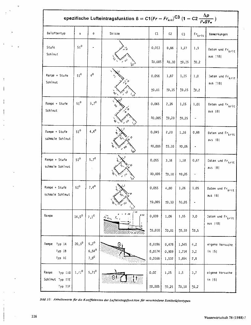
5. Summary and Outlook

Currently we do not yet have any definitive formulas that take all listed phen—

omena into account for the exact calculation of air entrainment in a bottom aerator

and for the flow of the water—air mixture downstream of the aerator. Nonetheless, the

discussion introduced here indicates that satisfactory calculations can be made for

practical air entrainment conditions for a large number of different bottom aerator

geometries (Figure 10) using an empirical air entrainment function [5] that accounts

for air flow in the bottom aerator. It is also possible to use standard hydraulic cal—

culation procedures for the section—by—section description of the influence of bottom

aeration on flow downstream of the bottom aerator. In this context, it is definitely

significant that water flow with bottom aeration exhibits higher flow velocities than

flow without bottom aeration.

In closing, it is important to note that neither the air entrainment mechanism

nor flow behavior of the water—air mixture downstream of the bottom aerator has yet

been adequately researched and that appropriate calculation procedures still need to

be developed for this purpose. Consequently, studies using hydraulic models will re—

main an important aid in finalizing spillway designs, but the design concept described

here can significantly shorten the draft phase.

19

SPECIFIC AIR ENTRAINPENT FUNCTION B = Cl (Fr - Fcri C3 (1 - Ap C2

P.9Y. )

AERATOR TYPE a± SKETCH Cl C2 C3 Fr

crit COPPENTS

STEP

BOTTCM GROOVE

51° ,. ...+

l-- 5,

0,013

10,005

- from

0,86

r0,10

1,27

10,15

1,9

.10,2

DATA & Frcrit

[18]

Rreft3 + STEP[

8071OM GROOVE

510 40

\ •

..1,

. t'' In.

0,056

1'0,01

1,87

10,15

1,15

10,15

1,0

10,2

DATA & Frcrit

from [18]

RAPP + STEP

BOTTOM GROOVE

51° 5,7°

+

. '

0,065

±.0,005

2,35

10,20

1,15

10,15

1,01 DATA & Ercrit

from

RAPP + STEP

NARROW

BOTTOM GROOVE

51° 4,4° ,.:

t,

‘ ,,•''4,":'

.

. •1P s»

0,045

±0,005

2,20

1'0,10

1,16

1:0,05

0,68 DATA & Frcrit .

from [8]

NARROW

BOTTOM GROOVE

RAM P + STEP 51° 5,7° c 1. . ,,• .

s 'i., 4,-,

:

0,055

10,005

3,16

10,10

1,18

±0,05

0,67

-

DATA & Frcrit

from [8]

RAPP + STEP

NARROW

BOTTOM GROOVE

510 7,4° s . . .., -...-, ,,..

.

i .

0,055

1.0,005

4,00

1.0,10

1,26

±0,05

1,05 DATA & Frcrit

from [8]

RAMP 14,5° 7,1°

•• • '

IS „, 2L, , 0 20, co 0,039

1.0,010

1,06

1'0,01

1,55

1,0,10

3,0

10,5

DATA & Frcrit,

from [18]

RAN13 TYPE IA

TYPE 15

TYPE IC

20,3° 5,2°

6,54°

7,9°

0

: - .

0,0196

0,0174

0,0168

0,478

0,909

1,532

1,565

1,714

1,854

4,2

3,2

2,8

AUTHOR'S OWN

TESTS IN

[5] ,

RAPP TYPE [10

BOT. TYPE IIE

GROOVE TYPE [IF

1,71° 5,71° 0,02

10,005

1,25

.4:0,25

1,5

1.0,10

3,7

1.0,2

AUTHOR'S OWN

TESTS IN

[51 t t

•

Figure 10: Reference values for the coefficients of the air entrainment function for various types of bottom aerators

20

Bibliography

[1] Aksoy, Sahap, Ethembabaoglu, Sakir. "Cavitation Damage at the Discharge Channels of Keban Dam," 13th ICOLD Congress, New Delhi, 1979.

[2] Hamilton, W.S. "Preventing Cavitation Damage to Hydraulic Structures," Water Power & Dam Construction, Nov., Dec. 1983, Jan. 1984.

[3] Kobus, H. "Local Air Entrainment and Detrainment," IAHR Symposium on Scale Effects in Modelling Hydraulic Structures, Esslingen am Neckar, Sept. 1984, Paper 4.10, Proceedings (Editor: H. Kobus).

[4] Kobus, H. "An Introduction to Air-water Flows in Hydraulics," Mitteilungen Institut Mr Wasserbau, Universiat Stuttgart, Vol. 61, October 1985.

[5] Koschitzky, H.P. "Dimensionierungskonzept fur Sohlbeltifter in Schutirinnen zur Vermeidung von Kavitationsschaden" ["Design Concept for Bottom Aerators in Spillways for Prevention of Cavitation Damage"], Mitteilungen Institut fiir Was-serbau, Universitat Stuttgart, Vol. 65, July 1987.

[6] Koschitzky, H.P., B. Westrich, H. Kobus. "Effects of Model Configuration, Flow Conditions and Scale in Modelling Spillway Aeration Grooves," IAHR Symposium on Scale Effects in Modelling Hydraulic Structures, Esslingen am Neckar, Sept. 1984, Paper 4.4, Proceedings (Editor: H. Kobus).

[7] Koschitzky, H.P., B. Barczewski, "Theoretische und experimentelle Vorstudien zur Frage des Lufteintrags und Lufttransports an Sohlbelliftern in Hochge-schwindigkeitsstromungen. Zwischenbericht zum DFG-Forschungs-vorhaben 'Lufteintrag an Sohlbeluftern" ["Theoretical and Experimental Preliminary In-vestigations on the Question of Air Entrainment and Air Transport at Bottom Aerators in High-speed Flow. Preliminary Report to the DFG [German Research Institute] Project 'Air Entrainment in Bottom Aerators," Wissenschaftlicher Bericht HWV No. 089, Institut Mr Wasserbau, Universitat Stuttgart, 1987.

[8] Low Heng Seng. "Model Studies of Clyde Dam Spillway Aerators: Research Report 86-6." Department of Civil Engineering, University of Canterbury Christchurch, New Zealand, March 1986.

[9] Miller, D.S. Internal Flow Systems. BHRA Fluid Engineering Series, Vol. 5, 1978.

[10] Minor, E. "Erfahrungen mit Schularinnenbeliiftung" ["Experience with Spillway Aeration"], 7th German Dam Symposium, March, 1987; Special edition of Wasser-wirtschaft, Vol. 6, June 1987.

[11] Minor, E. "Der Grundablai3 der Wasserkraftanlage Alicura in Argentinien" ["The Sluiceway at the Alicura Power Plant in Argentina"], 7th German Dam Sympo-sium, March, 1987; Special edition of Wasserwirtschaft, Vol. 6, June 1987.

[12] Naudascher, E. "Kavitationsprobleme in Grundablassen" ["Cavitation Problems in Sluices"], Wasserwirtschaft 72, Vol. 3, 1982.

[13] Peterka, A.J., "The Effect of Entrained Air on Cavitation Pitting," IAHR/ASCE Proceedings, Minnesota International Hydraulics Convention, Minneapolis, Minnesota, Sept. 1953.

21

Bibliography, cont.

[14] Pinto, H.L., "Model Evaluation of Aerators in Shooting Flow," IAHR Symposium on Scale Effects in Modelling Hydraulic Structures, Esslingen am Neckar, Sept. 1984, Paper 4.2, Proceedings (Editor: H. Kobus).

[151 Russel, S.O., G.J. Sheehan, "Effect of Entrained Air on Cavitation Damage," De-partment of Civil Engineering, University of British Columbia, Canadian Journal of Civil Engineering, Vancouver, 1974.

[16] Rutschmann, P, "Die transversale Druckverteilung unter Sprungstrahlen von SchuBrinnenbeluftern Folgen ftir den Lufteintrag" ("The Transverse Pres- sure Gradient under Shooting Flow in Spillway Aerators -- Consequences for Air Entrainment"), Wasserwirtschaft, Vol. 5, 1987.

[171 Rutschmann, P., P. Volkart, I.R. Wood, "Air Entrainment at Spillway Aerators," 9th Australasian Fluid Mechanics Conference, Auckland, Dec. 1986.

[18] Tan, P., "Model Studies of Aerators on Spillways," Research Report No. 84-6, University of Canterbury Christchurch, New Zealand, Feb. 1984.

[19] Vischer, D., "Kavitationen in SchuBrinnen" E"Caviation in Spillways"], 7th Ger-man Dam Symposium, March, 1987; Special edition of Wasserwirtschaft, Vol. 6, June 1987.

[20] Volkart, P., "Sohlenbeltiftung gegen Kavitationserosion in SchuBrinnen" ["Bottom Aeration to Prevent Cavitation Erosion in Spillways"], Wasserwirt-schaft 74, Vol. 9, Sept. 1984.

[21] Volkart, P., P. Rutschmann, "Air Entrainment Devices (Air Slots)," Mitteilungen der Versuchsanstalt fUr Wasserbau, Hydrologie und Glaziologie an der ETH Zurich, Vol. No. 72, 1984 (Editor: D. Vischer).

[22] Wood, I.R., "Air Water Flows," 21st IAHR Congress, Melbourne, Australia, Aug. 1985.

Address of the author: Dr.-Ing. Hans-Peter Koschitzky, Institut ftir 'Wasserbau, Universitat Stuttgart, Pfaffenwaldring 61, 7000 Stuttgart 80.

22

Hans-Peter Koschitzky

Kurzfassung / Abstract

Fiir den Entwurf und die hydraulische Dimensionierung von Sohlbeliiftern in Schuilrinnen wird em n Dimensionierungskon-zept vorgestellt, die Vorgehensweise bei der Dimensionierung wird erlautert. Den Schwerpunkt bildet die Dimensionierung eines Sohlbeliifters. Die hierzu erforderliche Lufteintrags-funktion wurde ftir verschiedene Beltiftergeometrien durch hydraulische Modellversuche und anhand veroffentlichter Daten bestimmt. Far die &mittlung des Gesamtlufteintrags unter Beriicksichtigung der Interaktion zwischen Wasserstr6-mung und LuftstrOmung im BeRifler wird em n Berechnungs-ansatz vorgestellt. Die Veranderung der Stromung durch den Einbau von Sohlbeltiftern wird diskutiert und Ansatze ftir deren Abschatzung aufgezeigt.

A design procedure for spillway aerators to prevent cavita-tion damages is presented and the design steps are explained. Necessary air entrainment functions for the design of differ-ent aerator geometries are given on the basis of hydraulic model investigations and of published data. A calculation method for the determination of the total air entrainment is given which considers the interaction between the water flow in the spillway and the air flow in the aerator. The influence of the aeration on the high-speed flow is discussed and calcu-lation estimates are given.

1 Vorbemerkungen

Durch Hochgeschwindigkeitsstromungen, wie sie in Beton-schuBrinnen und Grundablassen auftreten, kann es durch Kavitation und die damit einhergehende Kavitationserasion innerhalb kurzer Zeit zu erheblichen Schaden an Anlagen kommen. Zahlreiche Schadensfalle bestatigen dies [1,2, 10, 12].

Eine wirkungsvolle und heute auch an zahlreichen Anlagen bereits praktizierte MOglichkeit zur Vermeidung dieser Sella-den stellt die Beltiftung der StrOmung mit Hilfe von Sohlbe-liiftern dar. Die hierbei zur Anwendung kommenden Beliifter-geometrien sind zum Beispiel in [5, 21] umfassend dargestellt.

Bis heute ist zwar wissenschaftlich nicht eindeutig geklart, auf welche Weise die dem Wasser beigemischte Luft die Kavi-tationsschaden verhindert, es ist aber seit langem bekannt, dak. bereits 5% bis 8% Luftgehalt [13] ausreichend sind, urn Kavitationsschaden zu vermeiden. Mehr noch zeigte Russel [15], dal?) selbst Schaden, die an Betonproben ohne Luftzu-gabe in einem Kavitationskanal bei 46 m/s innerhalb einer halben Stunde entstanden waren, an gleichen Proben nach Beimischung von 5 % Luft, selbst nach einer Betriebszeit von zwei Stunden, nicht mehr entstanden.

Die Wirksamkeit der Sohlbeliiftung wird auch durch Erfahrun-gen an Naturausftihrungen bestatigt [2, 14]; so berichtet Minor [11] von einem betonierten Grundabla13, der nahezu em n Jalu lang mit Stromungsgeschwindigkeiten von tiber 40 m/s im FreispiegelabfluB betrieben wurde, ohne Kavita-tionsschaden zu zeigen.

Allerdings darf nicht verschwiegen werden, daB es auch Anla-gen gibt, die zwar im Hinblick auf die gewiinschte Kavita-

tionsvermeidung zuverlassig arbeiten, aber durch zuviel einge-mischte Luft em unerwiinschtes Abflui3geschehen zeigen. So kann zuviel eingemischte Luft die Wassertiefe ithermailig ver-graern, was insbesondere bei Grundablassen vermieden wer-den muB. AuBerdem wurde der Tatsache, dalS durch die ein-gemischte Luft die Stromung im Vergleich zur Klarwasser-stromung schneller wird [5, 22], bisher offensichtlich nicht ausreichend Rechnung getragen, wie auch Ausfiihrungen in [10] bestatigen.

2 Ben6tigte Entwurfsgrundlagen

Bei der Dimensionierung von SchuBrinnen mit Sohlbeliiftern mull ftir eine vorliegende Anlagensituation der Sohlbeliifter-typ, dessen Einbauort, der Beliifterabstand, die Anzahl und das Luftzufuhrsystem festgelegt werden. Dariiber hinaus mull die Veranderung des Abflul3geschehens in der SchuiSrinne durch den Einbau der Beliifter abgeschatzt und insbesondere die Auswirkungen der Beliiftung auf die anschlieBende Ener-gieumwandlungsanlage beriicksichtigt werden.

Hierftir wurde em Dimensionierungskonzept erarbeitet [5], dessen Hauptbestandteile in Bild 1 dargestellt sind. Dabei

i AUSGANGSDATEN Hydrologie; Topographie: etc.

HYDRAULISCHE BERECHNUNG DER SCHUSSRINNENSTROMUNG

Wasserspiegelverlaue StrOmungsgeschwindigkeiten; Froudezahlen; Grenzschichtentwicklung

ABSCHATZUNG DER KAVITATIONSGEFAHR

Vermeidung von Kavitationsschaden durch Sohlbelatung

VORENTWURF DES SOHLBELOFTERS Position des SohlbelUtters;

Belaftergeometrie: Luftzuluhrsystem

HYDRAULISCHE DIMENSIONIERUNG DES SOHLBELCIFTERS

Lultaufnahme bei verschiedenen AbftuBzustanden Abmessungen von Sohlbelafter und Luftzufuhrsystem

BERECHNUNG DER NACHFOLGENDEN SCHUSSRINNENSTROMUNG

Wirkungslange des BelOfters; Wassertielen und Stremungsgeschwindigkeiten; Luftkonzentrationen

Dimensionierung von SchuBrinnenbeliiftern The Design of Spillway Aerators

Traweita Priut* Lvit. Diff.4#44- 7,....-a Dem,

Team No. Book No. Paper No.

Bild Bausteine des Dimensionie-rungskonzeptes

ENDGOLTIGER ENTWURF UND HYDRAULISCHE BERECHNUNG

DER SCHUSSRINNE

220 Wasserwirtschaft 78 (1988) 5

Luttzutuhrsystem I Ausschnitt tar zweidimensionale 1?etrachtung

Atmospharendruck

,.......i..... Sox hleinbau

Unterdruck Ap

2

P < Patm

spezitischer lutteintrag (h.

Wasser-Lutt-Gemisch

EintrMsflache A. Eintnttstlacht

Typ I: Rampe Typ II: Rampe mit

Sohlnut

Lultzufuhr

\

luftzuluhr

77

in m'is qw in m2/s Fr yw in m tp in Pa pw in kg/m3 g in m/s2

mit: wird sowohl auf die Berechnung der Scharinnenstromung ohne Sohlbeliiftung, als auch auf die Abschatzung der Kavita-tionsgefahr entlang des F1ie13weges, die verschiedenen Ma13-nahmen zur Vermeidung von Kavitationsschaden u•ad auf die Veranderung der SchuBrinnenstromung durch die F..ohlbeliif-tung eingegangen. Der Schwerpunkt liegt auf dem Entwurf und der hydraulischen Dimensionierung der Sohlbeliifter, worth mit Hilfe von hydraulischen Modellversuchen em n Be-rechnungsansatz aufgestellt wurde, der die Interaktion zwi-schen der Luftstromung im Sohlbeliifter und der Wasserstro-mung in der SchuBrinne berticksichtigt.

3 Lufteintrag an einem Sohlbehifter

Ein Sohlbeliifter (Bild 2) besteht aus zwei Hauptelementen. — der Sohleinbau (oft als Sohlbeliifter bezeichnet) — das Luftzufuhrsystem.

Gesamtlutteintrag Q,

Bild 2: Prinzipskizze eines Sohlbeliifters

Jedes Teilsystem fur sich gesehen, hat seine eigene Str6mungs-charakteristik [3,4,6]. Analog wie bei Rohr-Pumpenkenn-linien wird der Schnittpunkt dieser beiden Charakteristiken in einem QL - Ap Diagramm oft als Arbeitspunkt bezeichnet [16,20].

Bei einer Veranderung der Wasserstromung, zum Beispiel durch Zunahme des Abflusses, verschiebt sich dieser „Arbeits-punkt" und somit andert sich auch der Unterdruck und die Luftstromung. Erschwerend kommt hinzu, dai3 der Unter-druck — hervorgerufen durch die Luftstr6mung im Sohlein-bau — in Rinnenquerrichtung nicht konstant ist [5,14,16]. Das heiBt, daf, selbst bei konstanter Wasserstromung der Ar-beitspunkt in Rinnenquerrichtung variiert und somit der spe-zifische Lufteintrag qL km2/s1 in Rinnenquerrichtung nicht konstant ist. Diese Interaktion zwischen Luft- und Wasserstro-mung mu13 bei der Ermittlung des Lufteintrags an Sohlbeliif-tern beriicksichtigt werden.

3.1 Zweidimensionale Lufteintragsfunktion

Zur Frage der Physik des Lufteintrags gibt es zwar grundsatz-liche Oberlegungen [3] und Gedankenmodelle [5, 7], eine Moglichkeit, den Lufteintragmechanismus formelmailig exakt zu beschreiben, gibt es aber noch nicht. Wegen der Komplexi-tat dieses Problems ist hiermit in naher Zukunft auch nicht zu rechnen. Deshalb mu l3 versucht werden, empirische An-satze zu entwickeln. Aufgrund dimensionsanalytischer Ober-legungen kann gezeigt werden, dai3 die Lufteintragsrate L flir eine Sohlbeliiftergeometrie als Funktion der Froudezahl Fr der Wasserstr6mung und eines dimensionslosen Druckparameters Ap/pw • g • yw dargestellt werden kann:

13 = qL/qw = f (Fr; Ap/pw• g • yw ) (bei gegebener Geometrie)

(1)

Wasserwirtschaft 78 (1988) 5

= spezinsener Luitemtrag = spezifischer Abflull = Froudezahl = vw/sig yw = Klarwassertiefe = Unterdruck im Sohlbeliifter = Dichte des Wassers = Normalfallbeschleunigung

Zur Bestimmung der empirischen zweidimensionalen Luft-eintragsfunktion wurden umfangreiche Modellversuche an zwei Grundtypen von Sohlbeliiftern (Bud 3) durchgeftihrt. Typ I stellt eine Rampe dar ftir die Anwendung in steilen Rinnen, Typ II eine Sohlitut mit Rampe ftir flache Rinnen bzw. Grundablasse.

Typ tR ( run) o ( 0 ) Ao (cm2 ) s (m) t (m)

Rinnenneigung: 37 °A -'.-1' a = 20.300

IA 25,0 5,20 215,00 - -

IB 31,3 6,54 215,00 - -

IC 37,5 7,90 215,00 - -

Rinnenneigung: 3 °A ---- a = 1.72°

IID 40,0 5,71 312,50 75 225

I IE 50,0 5,71 312,50 75 225

I IF 50,0 5,71 250,12 100 175

Bild 3: Untersuchte Sohlbeinftertypen

Die Modellversuche wurden in einem zweidimensionalen Aus-schnittmodell durchgefiihrt, welches im Detail in [5,6] be-schrieben ist. Im Modell wurde der Unterdruck im Sohlbeliif-ter variiert und durch den Einsatz eines Geblases bis auf den Wert null reduziert. Damit konnte die Abhangigkeit der Luft-eintragsrate von der Wasserstromung

130 = f0 (Fr) (Mr Ap/pw • g • yw = 0) (2)

sowie bei gegebener Froudezahl die Anderung von IS mit dem Druckparameter

ilp = fp (Ap/pw • g • yw) (fur Fr = const.) (3)

ermittelt werden.

Die Auftragung der Ergebnisse in Bild 4 verdeutlichen, dal3 mit wachsender Froudezahl einerseits und mit abnelunendem

221

Typ IF: Rampe mit Soh!nut

-1.

Unterdruck dp

Atmospharendruck p,„„

• kleine Werte des Druckparameters

0.2

Fr„„= 3.5 grotto Werte des Ap Druckparameters

0.0 20 3.0 4.0 0.0 63 7.0 9 0 9.0 10.0 11.0 12.0 13.0 14.0

OS

0 Rinnenachse

oder

Seitenwand

Gesamtlufteintrag (30

T(

0.5 1,0 z/B

Wasserstromung Q.

C1L,I+1 s ezifischer Lufteintrag (IL *"

— 7CiLd li K

°L(6) = i•1 1,2

t-1 I Liz r.

Beliifterstromung

Schach

tstr

om

un

g

Verluste im

Luftschacht

entlang 1

Apo

mogliche Verluste in

1 der Beliifterstromung

Staudruck 2

pLVL,./2

APo

ApE, PL'0+21' APo

Apo 2

pLy0/2

Apo 1-to

‘plAP.

Bild 7: Definitionsskizze ffir die LuftstrOmungsberechnung

Froudezahl Fr [ - ] Biid 4: Abluingigkeit der Lufteintragsrate von der Froudezahl Fr der WasserstrOmung und dem Unterdruck im Sohlbeliifter

Betrag des Druckparameters andererseits die spezifische Luft-eintragsrate zunimmt. Darilber hinaus wird aus Bild 4 auch ersichtlich, dat em signifikanter Lufteintrag erst ab einem ge-wissen Wert der Froudezahl — als kritische Froudezahl Frkrit des Beliifters bezeichnet — beginnt. Letztere hangt von der Beliiftergeometrie ab.

Die Lufteintragsfunktion fur eine Beliiftergeometrie (L1,p = 0) kann somit durch den Ansatz:

Bo = Cl (Fr - Frkiit)C 3 (4)

beschrieben werden. Der Zusammenhang zwischen der Luft-eintragsrate und dem Unterdruck nach Gleichung (3) erwies sich in guter Naherung als linear [5], so dat er dargestellt wer-den kann als:

Bp = to - C2(Ap/pw • g • yw ) (5) wobei der Koeffizient C2 mit wachsender Froudezahl leicht zunimmt.

Auf Grund dieser Erkenntnisse ist es damit moglich, die zwei-dimensionale Lufteintragsfunktion fiir beliebige Froudezahlen und variablen Unterdruck im Sohlbellifter wie folgt darzu-stellen:

2o' Cl (Fr - Fria&C 3 ( 1 - C2Ap/p, • g • yw )

(6)

Typ II Rampe mit Sohlnut

0.7

g— r„ 1 t,

.5 q" 01 U

0.5

0.4

0.3

0 • 2

0. 1

0.0 0 . 0 0 0.2 0.3 0.4 0.5 0.6 0.7 0.8

gemessene Lufteintragsrate B E - Bad 5: Vergleich zwischen Messung und der mit der empirischen Lufteintragsfunktion berechneten Lufteintragsrate

Eine entsprechende Auswertung der Metdaten, wie sie bei-spielhaft fur den Beliiftertyp II im Bild 5 dargestellt ist, zeigt, dat mit diesem empirischen Ansatz der Lufteintrag zufrieden-stellend ermittelt werden kann.

Die Zusammenstellung der Koeffizienten fiir die Lufteintrags-funktion nach Gleichung (6) fur die in Bild 3 dargestellten Beliiftergeometrien zeigt Bild 6. Zusatzlich wurde die Auswer-tung mit konstantem Exponenten (C3 = 1,5) mit aufgenom-men.

spezifische Lufteintragsfunktion IS = Cl(Fr — Fr„,)C3 Ap

C2 (1 — ) P.9Y.

Sohlbehifter C3 vanabel C3 . 1,5 = const.

Typ Fr,„ Cl C3 C2 Cl C2

1 A 4,2 0,0196 1,565 0,4784 0,0205 0,0001

1 8 3,2 0,0174 1,714 0,9092 0,0228 0,0001

1 C 2,8 0,0168 1,854 1,5325 0,0247 0,0325

11 0 3,8 0,0238 1,437 1,0970 0,0197 1,0920

11 E 3,5 0,0182 1,585 1,3573 0,0212 1,3400

:: r 3,5 0,0253 1,500 1,4448 0,0253 1,4447

Bild 6: Koeffizienten fiir die Lufteintragsfunktion der untersuchten Sohlbeliiftergeometrien

3.2 Luftstromung im Sohlbeliifter

Die Luftstr6mung kann in zwei Abschnitte, die Schacht- und die Beliifterstromung, unterteilt werden. Diese sind im Bild 7 mit den zugehorenden Bezeichnungen und dem qualitativen Druckverlauf im Sohleinbau dargestellt.

gere

ch

ne t

e L

uftein

tra

gsr

ate

B [ —

]

13 Ap = Cl(Fr — Fr„.„)1' 5 (1 — C2— p.gy. )

Typ Ho, Zahlenwerte der

I Typ 11E, Koeffizienten • Typ 11F, siehe Elitd 6

3%

222 Wasserwirtschaft 78 (1988) 5

Untenlyvelryorl•Bung Irn Sehibplutter Typ IA

0.2 0.1 0. 4 0.5 0:6 0:7 0.0

Breitenyerhiltnis z/B —

Bild 8: Gemessene Unterdruckvertettung im Sohlbeliifter Typ I het variabler Schufirinnenbreite

andererseits die Verluste in der Bellifterstromung zu null ange-nommen werden kOnnen. Der Vtrlust in der Schachtstromung kann hingegen nicht vernachlassigt werden.

Die Modelluntersuchungen bestatigten auch, dati die Quer-schnittsflache fiir die Berechnung der Belilfterstromung als konstant angenommen und in guter Naherung hierfiir die Eintrittsflache Ao angesetzt werden kann [5].

3.2.3 Gesamtlufteintrag

Aufgrund der genannten Tatsachen kann bei bekannter Luft-eintragsfunktion nach Gleichung (6) der Unteraruckverlauf quer zur SchuBrinne im Sohleinbau abschnittsweise mit Hilfe der Energiegleichung bestimmt werden. Die Berechnung er-folgt schrittweise von der Rinnenwand bis zur Rinnenmitte mit der Kontrollbedingung, dai3 die Summe der pro Schritt-weite Az berechneten Lufteintragsraten qL,i gleich dem der Berechnung zugrunde gelegten Gesamtlufteintrag QL ist. Die iterativen Berechnung IdAt sich in die folgenden Schritte unterteilen:

1. Ermittlung eines Schatzwertes fur den Gesamtlufteintrag (QL = qL • B) aus Gleichung (6) mit einem angenomme- nen mittleren Unterdruck Ap (sinnvoller Wert 2,0 bis 8,0 kPa).

2. Bestimmung des Unterdrucks Apo im Eintrittsquerschnitt Ao nach Gleichung (7) und von ApB in Rinnenmitte (bzw. an der gegenilberliegenden Wand) nach Gleichung (8).

3. Ermittlung des Lufteintrags qL,1 filr eine festgelegte Schritt- weite Az nach Gleichung (6) mit dem Unterdruck Apo (siehe Bild 7).

4. Der Unterdruck Api ergibt sich aus der Summe des Stau-drucks (PL • vL,?/2) an der Stelle (i = 1) (Luftgeschwin-digkeit (vL3 = (QL - AzqL,I)/A0 )) und dem Unterdruck APB•

5. Bestimmung des Lufteintrags qL,i+1 aus Gleichung (6) mit dem im Punkt 4 berechneten Unterdruck; dann analoge Rechenschritte ab Punkt 3.

Der Berechnungsgang wird bis zu (z = B) fortgeflihrt und solange iteriert, bis (EqL,i = QL) ist. Dies kann mit Hilfe eines Taschenrechners oder eines Rechenprogramms einfach durchgefiihrt werden. Entscheidend hierbei ist, daB durch die Verwendung der Lufteintragsfunktion in Verbindung mit der Luftstromungsberechnung hier eine Kupplung der Wasserstr6-mung mit der Luftstromung erfolgt, die Interaktion dieser beiden Stromungen also beracksichtigt wird.

3.2.1 Schachtstr6mung

Als Schachtstromung wird die Luftstromung im Zufuhrsystem bezeichnet. Sie umfaik den Stromungsweg vom Eintritt ins Zufuhrsystem bis zum Eintrittsquerschnitt Ao in der SchuB-rinnenseitenwand. Entlang dieser Stromung ist der Luftdurch-flui3 konstant und gleich dem Gesamtlufteintrag QL. Die Schachtstromung kann nach den klassischen Methoden der Stromungsmechanik berechnet werden. Aus der Bernoulli- Gleichung ergibt sich fur den Unterdruck im Eintrittsquer-schnitt Ao:

Apo = pLvL,02 /2 (X1/4rhy + tE + K + En + 1,0) (7) mit:

Verlustbeiwert fur den Einlauf-, Kriimmer- und tlbergangsverlust (far As = A0 ), bezogen auf den Eintrittsquerschnitt Ao

X Reibungsbeiwert nach Moody (X = f(4rhy/k5, Re)) rhy in m hydraulischer Radius des Luftschachtes 1 in m Flieliweg der Schachtstromung

Eine Abschatzung des Reibungsverlusts kann filr die tiblichen Naturabmessungen der Luftzufuhrsysteme mit den folgenden Werten vorgenommen werden:

7 hydraulischer Radius rhy: bei den vorkommenden Recht-eckquerschnitten mit Seitenverhaltnissen a:b von 1:1 bis 1:3 liegt dieser zwischen 0,25 a und 0,375 a und ist bei den gebrauchlichen Abmessungen der Luftschachte, in der Regel kleiner als 1,5 m.

— FlieBweg der Luft: im Bereich von 10 m bis 15 m. — Reynoldszahl: (Re = vj 4 rhy/PL) mit (vL > 20 m/s)

ist immer groBer 5•10°. — 4 rhy/ks: mit ks als aquivalenter Sandrauheit des Betons,

liegt zwischen 1300 und 13000.

Damit ergibt sich em n Reibungsbeiwert X zwischen 0,01 und 0,02 und em n Gesamtreibungsverlustbeiwert X1/4rhy zwischen 0,025 bis 0,05. lin Vergleich zu den Ortlichen Verlusten kann dieser in der Regel vernachlassigt werden. Die Verlustbeiwerte fur die ortlichen Verluste konnen aus der Literatur entnom-men werden, z.B. [9].

3.2.2 Beliifterstromung

Als BeliifterstrOmung wird die Luftstromung im Sohleinbau bezeichnet, welche quer zur Wasserstromung im Sohleinbau verlauft. Vom Eintrittsquerschnitt Ao bis zur Rinnenachse, bzw. bei einseitiger Beliiftung bis zur gegeniiberliegenden Seitenwand, nimmt der Luftdurchfluii wegen des Lufteintrags in die Wasserstromung vom Wert des Gesamtlufteintrags QL bis auf den Wert 0 ab, wodurch es zu einer ausgepragten Unterdruckverteilung in Querrichtung kommt.

Ausgehend von der Schachtstr6mungsberechnung sind so-wohl der Unterdruck Apo im Eintrittsquerschnitt Ao, der dynamische Druck pLvL,02/ 2 und somit auch der Druckver-lust bis zu Ao bekannt. linter der vereinfachten Annahme, dal die Verluste in der Beliifterstromung gegeniiber denen der Schachtstr6mung vernachlassigbar sind, kann der Unter- druck am Ende der Belafterstromung bestimmt werden zu (siehe Bild 7):

APB = APo - PL • vL,02/2 (8) Die der Gleichung (8) zugrunde gelegte Annahme wurde durch Modellversuche in einem dreidimensionalen Vollmo-dell einer Scharinne mit den Beliiftern nach Bild 3 besta-tigt [5]. Durch eine verschiebbare Trennwand wurde die Rinnebreite B variiert und fur verschiedene Abflui3zustande der Gesamtlufteintrag mit dem zugeharigen Unterdruckver-lauf gemessen.

Eine dimensionslose Darstellung der gemessenen Verteilungen (Bild 8) mit dem Unterdruck Ap0 im Eintrittsquerschnitt Ao und der jewelligen Rinnenbreite B als BezugsgroBe zeigt, dal3 einerseits der Verlauf unabhangig von der Rinnenbreite ist und

224 Wasserwirtschaft 78 (1988) 5

- 4 Auswirkungen der Sohlbeliftung aus die Wasserstromung

Neben dem erwiinschten Kavitationserosionsschutz fiihrt der Einbau eines Sohlbeliifters und die eingetragene Luft zu Ver-anderungen in der Str6mung, die beim Entwurf der Schufl-rinne und insbesondere der anschlieBenden Energieumwand-lungsanlage berticksichtigt werden miissen.

4.1 Hydrodynamische Belastung im Strahlauftreffpunkt

Durch den Sohlbeinbau wird em n sich von der Sohle abheben-der Wasserstrahl erzeugt, der je nach Geometrie des Belilfters zwischen 10 m und 25 m weit springt, bis er wieder auf der Rinnensohle auftrifft. Dies fart zu hydrodynamischen Bela-stungen im Bereich des Auftreffpunktes, deren Gr&e und Schwankungen den hydrostatischen Wasserdruck deutlich iibersteigen kOnnen, Beispiele sind in [5] dargestellt.

4.2 Beginn der OberflOchenbeliiftung am Sohlbeliifter

Aus Natur- und" Modellbeobachtungen ist bekannt, dafl bei Sohlbeliiftern mit Deflektoren unmittelbar am Beliifter die Oberflachenbeliiftung beginnt. Dies riihrt vermutlich daher, da.6 es im Wasserstrahl unmittelbar nach dem Verlassen der Rampe zu einer schlagartigen Druckumlagerung kommt. Ver-gleichbar einer plotzlichen Erweiterung in einer Rohrstromung ist damit eine zusatzliche Turbulenzproduktion verbunden, was dann die Selbstbeliiftung an der Oberflache auslosen kann. Pinto [14] gibt aus Naturbeobachtungen an, dafl die dadurch hervorgerufene Oberflachenbeliiftung in der SchuB-rinne in Foz do Areia Werte bis zu 48% erreicht hat, was weit iiber den Werten flir die zu erwartende Oberflachenbe-liiftung ohne Sohlbeliifter lag, die rechnerisch zudem erst weiter stromab einsetzen

4.3 Vergrofierung der Wassertiefe durch die eingemischte Luft

Unterstrom des Sohlbeliifters nimmt infolge des Lufteintrags am Sohlbeliifter wie auch durch die einsetzende Oberflachen-beliiftung die Wassertiefe zu. Dieser Effekt, beim Problem der Selbstbeliiftung als das sogenannte „bulking" bezeichnet, kann in erster Naherung unter der Annahme, daiS die Stro-mungsgeschwindigkeit des Wasser-Luft-Gemisches vwL gleich der Stromungsgeschwindigkeit der Klarwasserstromung vw ist, abgeschatzt werden zu:

YwL = (1/(1-F))31w (9)

mit: yw = Klarwassertiefe ohne Luftanteil = tiefengemittelte Luftkonzentration

Legt man als untere Grenze fiir die Ermittlung der Gemisch-wassertiefe nur die Lufteintragsrate zugrunde, kann Glei-chung (9) dargestellt werden als:

YwL = (1 + B)Yw ( 10)

woraus sich em n Anhaltswert fur die Wassertiefe ergibt, welcher bei der Festlegung der Seitenwandhohe zu beriicksichtigen ist.

4.4 Gischtbildung an der Wasseroberfldche

Die Sohlbeliiftung, verbunden mit der einsetzenden Oberfla-chenbeliiftung, fiihrt unterstrom der Bellifter oft zu mittleren Luftkonzentrationen, die weit ilber den maximalen Gleichge-wichts-Transportkonzentrationen der Wasserstromung liegen. Daher kommt es zum Luftaustrag an der Wasseroberflache, verbunden mit einer starken Wassernebel- und Gischtbildung, welche auch in k1einma13stab1ichen Modellversuchen beobach-tet werden kann. Dies ist zusatzlich bei der Festlegung der SeitenwandhOhe zu beriicksichtigen.

4.5 Energieverlust durch den Lufteintrags-Vermischungs- und Transportprozeft

Sowohl der Lufteintragsproze13 entlang des Sprungstrahls als auch der Vermischungs- und Transportprozei3 in der Wasser-Luft-Gemischstromung unterstrom des Sohlbeliifters, benoti-

Wasserwirtschaft 78 (1988) 5

gen Energie, welche folglich der WasserstrOmung entzogen werden mull. Ein Vergleich der kinetischen Energie der SchuArinnenstromung mit der maximalen kinetischen Energie der Luftstromung im Sohlbeliifter zeigt, dat diese selbst bei extrem groBen Lufteintragsraten 1 nur 0,5% bis 1% der Was-serstromung betragt. Dies bedeutet, der durch den Luftein-tragsprozefl hervorgerufene Energieverlust betragt maximal 0,5% bis 1% der kinetischen Energie der SchuBrinnenstro-mung. Er ist somit vernachlassigbar.

Analoges gilt fur den Energieverlust zufolge des Luftvermi-schungs- und Transportprozesses. Die Gro1e dieses Energie-verlustes fur den hier vorliegenden Fall einer nicht gleichfOr-migen Str6mung mit sich in FlieBrichtung verandernden Luftkonzentration, ist heute zwar noch nicht erforscht und daher nicht eindeutig anzugeben, eine Abschatzung der GrO-Benordnung [5] mit Hilfe der Erkenntnisse fur eine gleichfor-mige StrOmung mit Oberflachenbeliiftung zeigt aber, da13 dieser Energieverlust bei der hydraulischen Dimensionierung ebenfalls vernachlassigt werden kann. Damit liegt man, ins-besondere auch in Hinblick auf die Dimensionierung der Energieumwandlungsanlage, auf der sicheren Seite.

4.6 Erheihte Beschleunigung entlang der Sprungweite

Entlang des Sprungwegs des Wasserstrahls am Sohlbeliifter fehlt an der Strahlunterseite die Stromungsberandung. Da-durch wirkt der Stromung in diesem Bereich, von den beiden Seitenwanden abgesehen, keine Wandreibung mehr entgegen. Das heiBt, die Stromung erfahrt entlang des Sprungwegs eine erhohte Beschleunigung. Dieser kann naherungsweise dadurch Rechnung getragen werden, da13 nach vorheriger Bestimmung der Strahlsprungweite [5], der Sohlreibungsverlust entlang dieser verringert bzw. zu Null angesetzt wird.

4.7 Erhohte Beschleunigung durch die Reduktion der Sohlschubspannung

Unterstrom des Auftreffpunktes sind an der Sohle hohe Luft-konzentrationen vorhanden, die zwar mit fortschreitender FlieBrichtung abnehmen, aber allein schon aus der Forderung der zur Kavitationsvermeidung ben6tigten Mindestkonzentra-tion an der Sohle, nicht unter Werte von 5% bis 8% absinken sollen. Die dadurch hervorgerufene Verringerung des Reibungs-beiwertes fiihrt ebenfalls zu einer erhohten Beschleunigung der Stromung, wie durch die folgenden Oberlegungen gezeigt werden kann. Fiihrt man in die Definition der Sohlschub-spannung:

Ts = (Xw/8) (Pwvw2 ) (11)

mit: Xw Reibungsbeiwert nach Moody

an Stelle der Dichte pw des Wassers die Dichte pw,L des Wasser-Luft-Gemisches, welche vereinfacht angesetzt werden kann zu:

Pw,L = pw(1 - (12)

gleichformige StrEimung I

1,0 0,0

0,8

iaT) 0,02 0,6

0,4 0,01

e"i2 8 0,2 tietengemittelte Gleichgewichts-

transportkonzentration C" in % °

0 10 20 30 40 50 60 70

cs< 2 % I I

15 38 48 58 65 zugehorige Sohlkonzentration c, in %

Bild 9: Abhangigkeit des Rauheitsbeiwenes von der Luftkonzentration

225

Ver

ha

ltnis

de

r R

eib

ung

sbeiw

erte

spezifische Lufteintragsfunktion B = Cl (Fr - Fr„it )C3 (1 -

,

Ap C2 P.gYw )

BelUftertyp a a Skizze Cl C2 C3 Frkrit Bemerkungen

Stufe

Sohinut

51° - c4

c p

L__ 51°

0,013

t0,005

0,86

t0,10

1,27

10,15

1,9

t0,2

Daten und Frkr t

aus 1181

Rampe + Stufe

Sohlnut

51° 4° l P

, ,

c,

, .

is • ,sr.

0,056

+0,01

1,87

10,15

1,15

10,15

1,0

10,2

Oaten und Frkrit

aus 1181

Rampe + Stufe

Sohlnut

51° 5,7° ,e :

.',,

'"P is

. -,

0,065

t0,005

2,35

10,20

1,15

t0,15

1,01

-

Daten und Frkrit

aus 181

Rampe + Stufe

schmale Sohlnut

51° 4,4° c •

+0 • is

' ,...-

r

0,045

±0,005

2,20

t0,10

1,16

t0,05

1

0,68

-

Oaten und Frkrit

aus 181

Rampe + Stufe

schmale Sohlnut

51° 5,7° t• c 4

+

,

L_ 5r

0,055

t0,005

3,16

10,10

1,18

±0,05

0,67

-

Daten und Frkrit

aus 181

Rampe + Stufe

schmale Sohlnut

51° 7,4° i '

...-f, '''\ .4)

\ _

r

0,055

t0,005

4,00

t0,10

1,26

t0,05

1,05

-

Daten und Frkrit

aus 181

Rampe 14,5o 7,1° t

-'se, A, a 0 2

0!

4 I I

iso

1 1 j

,

050 0,039

1:0,010

1,06

"10,01

1,55

+0,10

3,0

t0,5

Daten und Frkrit

aus 1 181 i

, 7/MV2ti

Rampe Typ IA

Typ IB

Typ IC

20,3° 5,2°

6,54°

7,90

0

-

..

0,0196

0,0174

0,0168

0,478

0,909

1,532

1,565

1,714

1,854

4,2

3,2

2,8

eigene Versuche

in 151

-

Rampe Typ LID

Sohlnut Typ LIE

• Typ IIF

1,71° 5,71° MI.% 0,02

t0,005

1,25

t0,25

1,5

-10,10

3,7

+0,2

eigene Versuche

in 151 f di Al

Bild 10: Anhaltswerte fir die Koeffizienten der Lufteintragsfunktion fir verschiedene Sohlbeliiftertypen

226 Wasserwirtschaft 78 (1988) 5

ein und benicksicnngt auseruem, LI4110 Itil 1 /4“,

nung nur die sohlnahe Luftkonzentration cs von Bedeutung ist, folgt aus den Gleichungen (11) und (12), far die Sohl-schubspannung des Wasser-Luft-Gemisches:

rs,wL = (Xw/8) • (Pw(1- cs) vw2) (13)

Das Verhaltnis der Sohlschubspannungen zwischen der Klar-wassertiefe und der Wasser-Luft-GemischstrOmung und somit der Reibungseinflui3 kann damit dargestellt werden als:

rs,wL / Ts (1 Cs ) (14)

Dies zeigt, daii mit zunehmender Luftkonzentration der Rei-bungseinfluii an der Sohle zurtickgeht, somit die Stromung eine erhohte Beschleunigung erfahrt. Eine Abschatzung dieses Effekts ist mit Hilfe der Arbeit von Wood [22] mOglich, der die Abhangigkeit des Reibungsbei-wertes von der tiefengemittelten Gleichgewichtstransportkon-zentration in einer gleichformigen Striimung angibt (BO 9). Erganzt man die zu diesen mittleren Luftkonzentrationen zugehOrenden Sohlkofizentrationen cs als zusatzliche Achse in Bild 9 ist festzustellen, daS sich zwar erst ab mittleren Konzentrationen a- von tiber 30% der Rauheitsbeiwert deut-lich verringert, hierzu aber deutlich geringere Sohlkonzentra-tionen gehiiren. Bereits ftir die Mindestsohlkonzentrationen von nur 5% ist die Veranderung des Reibungsbeiwerts deut-lich sichtbar. Da die tatsachlichen Sohlkonzentrationen aber iiber weite Strecken erheblich iiber diesen 5% liegen, ist ein-sichtig, daS insbesondere im Fall von mehreren hintereinander liegenden Sohlbelliftern der durch die Verminderung der Sohl-reibung hervorgerufene Beschleunigungseffekt von Bedeutung ist. Das heist, die Schufkinnenstromung wird schneller als ohne Sohlbelfiftung, was die in [10] gemachten Naturbeob-achtungen erklart. Mit Hilfe von Bild 9 ist es damit moglich, bei Kenntnis der Luftaufnahme im Sohlbeliifter (siehe Punkt 3) StrOmungs-geschwindigkeiten unterstrom des Auftreffpunktes abzuschat- zen.

5 Zusammenfassung und Ausblick

Fiir die exakte Berechnung des Lufteintrags an einem Sohl-beliifter und der Wasser-Luft-Gemisch-Striimung unterstrom des Beliifters, unter Berticksichtigung aller aufgeftihrten Phan-omene, liegen heute noch keine geschlossenen Ansatze vor. Die Ausfiihrungen zeigen aber, daS ftir praktische Belange der Lufteintrag ftir eine ganze Anzahl verschiedener Sohlbeliifter-geometrien (Bud 10) mit Hilfe einer empirischen Lufteintrags-funktion [5] unter Beriicksichtigung der Luftstriimung im Sohlbeliifter zufriedenstellend ermittelt werden kann. Ebenso kann unterstrom des Sohlbeliifters durch eine abschnittsweise Betrachtung mit Hilfe der bblichen hydraulischen Berechnungs-verfahren der Einflui3 der Sohlbeliiftung auf die Stromung er-fa2,t werden. Von entscheidender Bedeutung hierbei ist, (Jail eine WasserstrOmung mit Sohlbeiiiftung hohere Stromungs-geschwindigIceiten aufweist als ohne Sohlbeliiftung.

AbschlieBend sei darauf hingewiesen, dalS weder der Luftein-tragsmechanismus noch die Stromungsvorgange der Wasser-Luft-GemischstrOmung unterstrom von Sohlbeliiftern bisher geniigend erforscht sind und hierftir noch entsprechende Berechnungsverfahren entwickelt werden milssen. Daher wird auch weiterhin der hydraulische Modellversuch em n wichtiges Hilfsmittel bei der endgUltigen Dirnensionierung von Saha-rinnen bleiben, die Entwurfsphase kann aber mit Hilfe des aufgestellten Dimensionierungskonzeptes wesentlich verkiirzt werden.

[ 1] Aksoy, Sahap, Ethembabaoglu, Sakir: Cavitation damage at the discharge channels of Keban Dam. 13th ICOLD Congress, New Delhi, 1979

[ 2] Hamilton, W.S.: Preventing cavitation damage to hydraulic struc- tures. Water Power & Dam Construction, Nov., Dec. 1983, Jan. 1984

31 Kobus, H.: Local air entrainment and detrainment. IAHR Sym-posium on Scale Effects in Modelling Hydraulic Structures, Esslingen am Neckar, Sept. 1984, Paper 4.10, Proceedings (Editor: H. Kobus)

41 Kobus, H.: An introduction to air-water flows in hydraulics. Mitteilungen Institut ftir Wasserbau, Universitat Stuttgart, Heft 61, Oktober 198$

[ 5 Koschitzky, H.-P.: Dimensionierungskonzept flir Sohlbeltifter in Scharinnen zur Vermeidung von Kavitationsschaden. Mitteilun- gen Institut fiir Wasserbau, Universitat Stuttgart, Heft 65, Juli 1987

[ 61 Koschitzky, H.-P., B. Westrich, H. Kobus: Effects of model configuration, flow conditions and scale in modelling spillway aeration grooves. IAHR Symposium on Scale Effects in Model- ling Hydraulic Structures. Esslingen am Neckar, Sept. 1984, Paper 4.4, Proceedings (Editor: H. Kobus)

71 Koschitzky, H.-P., B. Barczewski: Theoretische und experimen- telle Vorstudien zur Frage des Lufteintrags und Lufttransports an Sohlbelaftern in HochgeschwindigkeitsstrOmungen. Zwischen- bericht zum DFG-Forschungsvorhaben „Lufteintrag an Sohl- beltiftern", Wissenschaftlicher Bericht HWV Nr. 089, Institut ftir Wasserbau, Universitiit Stuttgart, 1987

[ 81 Low Heng Seng: Model studies of Clyde Dam spillway aerators; Research report 86-6, Department of Civil Engineering, Univer- sity of Canterbury Christchurch, New Zealand, March 1986

[ 9] Miller, D.S.: Internal flow systems. BHRA Fluid Engineering Series, Volume 5, 1978

[10] Minor, E.: Erfahrungen mit SchuBrinnenbelaftung. 7. Deutsches Talsperren-SymPosium, Marz 1987; Sonderheft Wasserwirtschaft Heft 6, Juni 1987

[11] Minor, E.: Der Grundablail der Wasserkraftanlage Alicura in Argentinien. 7. Deutsches Talsperren-Symposium, Miirz 1987; Sonderheft Wasserwirtschaft, Heft 6, Juni 1987

[12] Naudascher, E.: Kavitationsprobleme in Grundablassen. Wasser- wirtschaft 72, Heft 3, 1982

[13] Peterka, A.J.: The effect of entrained air on cavitation pitting. IAHR/ASCE Proceedings, Minnesota International Hydraulics Convention, Minneapolis, Minnesota, September 1953

[14] Pinto, N.L.: Model evaluation of aerators in shooting flow. IAHR, Symposium on Scale Effects in Modelling Hydraulic Structures, Esslingen am Neckar, Sept. 1984, Paper 4.2, Proceed- ings (Editor: H. Kobus)

[15] Russel, S.O., G.J. Sheehan: Effect of entrained air on cavitation damage. Department of Civil Engineering, University of British Columbia, Canadian Journal of Civil Engineering, Vancouver 1974

[16] Rutschmann, P.: Die transversale Druckverteilung unter Sprung-strahlen von SchuBrinnenbeliiftern — Folgen fur den Lufteintrag. Wasserwirtschaft, Heft 5, 1987

[17] Rutschmann, P., P. Volkart, I.R. Wood: Air entrainment at spill- way aerators. 9th Australasian Fluid Mechanics Conference, Auckland, Dec. 1986

[18] Tan, P.: Model studies of Aerators on Spillways. Research re-port 84-6, Department of Civil Engineering, University of Can- terbury Christchurch, New Zealand, Feb. 1984

[19] Vischer, D.: Kavitation in Schatrinnen. 7. Deutsches Talsperren-Symposium, Marz 1987; Sonderheft Wasserwirtschaft, Heft 6, Juni 1987

[20] Volkart, P.. Sohlenbeliiftung gegen Kavitationserosion in Schuil- rinnen. Wasserwirtschaft 74, Heft 9, September 1984

[21] Volkart, P., P. Rutschmann: Air entrainment devices (air slots). Mitteilungen der Versuchsanstalt ftir Wasserbau, Hydrologie und Glaziologie an der ETH Ziirich, Heft Nr. 72, 1984 (Herausgeber: D. Vischer)

[22] Wood, I.R.: Air water flows. 21st IAHR Congress, Melbourne, Australia, Aug. 1985

Anschrift des Verfassers: Dr.-Ing. Hans-Peter Koschitzky, Institut fur Wasserbau, Universitat Stuttgart, Pfaffenwaldring 61, 7000 Stuttgart 80

Anzeigenschla fiir die Juni-Ausgabe, Schwerpunktthema: Gewasserpflege, am 23. Mai 1988

Anzeigenschlug -Mr die Doppelheft-Ausgabe Juli/August, Schwerpunktthema: Aktuelle Themen des Wasserbaus, am 24. Juni 1988

227 Wasserwirtschaft 78 (1988) 5