Embed Size (px)
Citation preview

Ozark-OuachitaHighlands Assessment
Air Quality
United StatesDepartment ofAgriculture
Forest Service
SouthernSouthernSouthernSouthernSouthernResearch StationResearch StationResearch StationResearch StationResearch Station
General TechnicalReport SRS-32
REPORT
2OF 5

Cover photo: Clear day in the Ozarks
Photo by A.C. Haralson, Arkansas Department of Parks and Recreation, Little Rock, AR.
Natural resource specialists and research scientists worked together to produce the five GeneralTechnical Reports that comprise the Ozark-Ouachita Highlands Assessment:
• Summary Report• Air Quality• Aquatic Conditions• Social and Economic Conditions• Terrestrial Vegetation and Wildlife
For information regarding how to obtain these Assessment documents, please contact: USDA ForestService, P.O. Box 1270, Hot Springs, AR 71902 or telephone 501-321-5202.
To limit publication costs, few color maps and figures were used in the Assessment reports. For colorversions of some of the Assessment figures and supplemental material, please see the Assessment’s homepage on the Internet at <http://www.fs.fed.us/oonf/ooha/welcome.htm>. The Assessment reports willbe online for about 2 years after the date on this publication; then they will be archived.
Please note: When “authors” are agency or business names, most are abbreviated to save space in thecitations of the body of the report. The “References” at the end of the report contain both the full nameand abbreviations. Because abbreviations sometimes are not in the same alphabetical order as the refer-ences, for clarifications of abbreviations, consult the “Glossary of Abbreviations and Acronyms.”
The use of trade, firm, or corporation names in this publication is for the information and convenience ofthe readers. Such use does not constitute an official endorsement of any product or service by the USDAForest Service.
December 1999
Southern Research StationP.O. Box 2680
Asheville, North Carolina 28802

Ozark-Ouachita Highlands Assessment:
Air Quality
Eastern RegionU.S. Department of Agriculture
Forest ServiceMilwaukee, WI
North Central Research StationU.S. Department of Agriculture
Forest ServiceSt. Paul, MN
Southern RegionU.S. Department of Agriculture
Forest ServiceAtlanta, GA
Southern Research StationU.S. Department of Agriculture
Forest ServiceAsheville, NC


Contents
Page
Preface . . . . . . . . . . . . . . . . . . . . . . . . . . . . . . . . . . . . v
Contributors to This Report . . . . . . . . . . . . . . . . . . vi
Acknowledgments . . . . . . . . . . . . . . . . . . . . . . . . . . viii
Executive Summary . . . . . . . . . . . . . . . . . . . . . . . . . ix
Chapter 1: Major Air Pollutants . . . . . . . . . . . . . . 1
Air Quality in the Assessment Area . . . . . . . . . . . . 1Primary Pollutants . . . . . . . . . . . . . . . . . . . . . . . . . . 1Key Findings . . . . . . . . . . . . . . . . . . . . . . . . . . . . . . 2Data Sources and Methods of Analysis . . . . . . . . . 2Patterns and Trends . . . . . . . . . . . . . . . . . . . . . . . . . 4
Particulate Matter . . . . . . . . . . . . . . . . . . . . . . . . 4Nitrogen Oxides . . . . . . . . . . . . . . . . . . . . . . . . . . 6Volatile Organic Compounds . . . . . . . . . . . . . . . . 8Sulfur Dioxide . . . . . . . . . . . . . . . . . . . . . . . . . . 10Pollution Exposure Index Results . . . . . . . . . . . 11Emission Trends . . . . . . . . . . . . . . . . . . . . . . . . . 12
Implications and Opportunities . . . . . . . . . . . . . . . 13
Chapter 2: Particulate Matter (PM10) in the Air . . . . . . . . . . . . . . 15
Key Findings . . . . . . . . . . . . . . . . . . . . . . . . . . . . . 16Data Sources and Methods of Analysis . . . . . . . . 16Patterns and Trends . . . . . . . . . . . . . . . . . . . . . . . . 17Implications and Opportunities . . . . . . . . . . . . . . . 20
Page
Chapter 3: Visibility . . . . . . . . . . . . . . . . . . . . . . . . 23
Key Findings . . . . . . . . . . . . . . . . . . . . . . . . . . . . . 24Data Sources and Methods of Analysis . . . . . . . . 24Patterns and Trends . . . . . . . . . . . . . . . . . . . . . . . . 25Implications and Opportunities . . . . . . . . . . . . . . . 31
Chapter 4: Ground-Level Ozone . . . . . . . . . . . . . 33
Key Findings . . . . . . . . . . . . . . . . . . . . . . . . . . . . . 34Data Sources and Methods of Analysis . . . . . . . . 34Patterns and Trends . . . . . . . . . . . . . . . . . . . . . . . . 36Implications and Opportunities . . . . . . . . . . . . . . . 38
Chapter 5: Acid Deposition . . . . . . . . . . . . . . . . . 43
Key Findings . . . . . . . . . . . . . . . . . . . . . . . . . . . . . 43Data Sources and Methods of Analysis . . . . . . . . 44Patterns and Trends . . . . . . . . . . . . . . . . . . . . . . . . 44Implications and Opportunities . . . . . . . . . . . . . . . 47
References . . . . . . . . . . . . . . . . . . . . . . . . . . . . . . . . 49
Glossary of Terms . . . . . . . . . . . . . . . . . . . . . . . . . 52
Glossary of Abbreviations and Acronyms . . . . 54
List of Tables . . . . . . . . . . . . . . . . . . . . . . . . . . . . . . 55
List of Figures . . . . . . . . . . . . . . . . . . . . . . . . . . . . . 56
iii


Preface
Change is evident across the Ozark and Ouachita Highlands. Whether paying attention to State andregional news, studying statistical patterns and trends, or driving through the Highlands, one cannot escapesigns that growth may be putting strains on the area’s natural resources and human communities. Howpeople regard these changes varies widely, however, as does access to reliable information that might helpthem assess the significance of what is happening in the Highlands. The Assessment reports providewindows to a wealth of such information.
The Air Quality report is one of five that document the results of the Ozark-Ouachita HighlandsAssessment. Federal and State natural resource agency employees and university and other cooperatorsworked together to produce the four technical reports that examine air quality; aquatic conditions; socialand economic conditions; and terrestrial vegetation and wildlife. Dozens of experts in various fieldsprovided technical reviews. Other citizens were involved in working meetings and supplied valuable ideasand information. The Summary Report provides an overview of the key findings presented in the fourtechnical reports. Data sources, methods of analysis, findings, discussion of implications, and links todozens of additional sources of information are included in the more detailed technical reports.
The USDA Forest Service initiated the Assessment and worked with other agencies to develop asynthesis of the best information available on conditions and trends in the Ozark-Ouachita Highlands.Assessment reports emphasize those conditions and trends most likely to have some bearing on the futuremanagement of the region’s three national forests—the Mark Twain, Ouachita, and Ozark-St. Francis.People who are interested in the future of the region’s other public lands and waters or of this remarkableregion as a whole should also find the reports valuable.
No specific statutory requirement led to the Assessment. However, data and findings assembled in thereports will provide some of the information relevant for an evaluation of possible changes in the land andresource management plans of the Highland’s three national forests. The National Forest ManagementAct directs the Forest Service to revise such management plans every 10 to 15 years, which means thatthe national forests of Arkansas, Missouri, and Oklahoma are slated to publish revised plans in the year2001. Due to restrictions in the 1998 appropriations bill that provides funding for the Forest Service, it isuncertain when these revisions can begin.
The charter for the Ozark-Ouachita Highlands Assessment established a team structure and listedtentative questions that the teams would address. Assembled in mid-1996, the Terrestrial, Aquatic andAtmospheric, and Human Dimensions (Social-Economic) Teams soon refined and condensed thesequestions and then gathered and evaluated vast quantities of information. They drafted their key findings inlate 1997 and refined them several times through mid-1999. In addition to offering relevant data and keyfindings in the reports, the authors discuss some of the possible implications of their findings for futurepublic land management in the Highlands and for related research. The Assessment reports, however, stopwell short of making decisions concerning management of any lands in the Highlands or about futureresearch. In no way do the reports represent management plans. Instead, the findings and conclusionsoffered in the Assessment reports are intended to stimulate discussion and further study.
v

Contributors to This Report
Assessment Team Leader
William F. Pell, Ecologist, USDA Forest Service, Hot Springs, AR
Aquatic-Atmospheric Team Leader
J. Alan Clingenpeel, Forest Hydrologist, USDA Forest Service, Ouachita National Forest, Hot Springs, AR
Authors
Chapter 1: Major Air Pollutants
William A Jackson
Chapter 2: Particulate Matter in the Air
Cliff F. Hunt, Warren E. Heilman
Chapter 3: Visibility
Cliff F. Hunt
Chapter 4: Ground-Level Ozone
William A Jackson
Chapter 5: Acid Deposition
Cliff F. Hunt, Warren E. Heilman
Author Information
Warren E. Heilman, Research Meteorologist, USDA Forest Service, North Central Research Station, EastLansing, MI.
Cliff F. Hunt, Air Resource Management Specialist (now retired), USDA Forest Service, National Forestsin Arkansas, Oklahoma, and Texas, Hot Springs, AR.
William A Jackson, Air Resource Management Specialist, USDA Forest Service, National Forests inNorth Carolina, South Carolina, and Tennessee, Asheville, NC.
vi

Other Contributors
The Cooperative Institute for Research in the Atmosphere (CIRA), Colorado State University, FortCollins, CO—two figures that include IMPROVE data.
Scott Copeland, Visibility Data Analyst, CIRA, Colorado State University, Fort Collins, CO—the visibilitydata analysis.
Jeffrey W. Grimm, Research Assistant, The Pennsylvania State University, University Park, PA—aciddeposition data modeling.
Janna E. Hummel, Environmental Engineer, E. H. Pechan & Associates, Inc., Durham, NC—emissionsdata.
Allen S. Lefohn, President, A.S.L. & Associates, Helena, MT—data to conduct the ground-level ozoneanalysis.
James A. Lynch, Professor of Forest Hydrology, The Pennsylvania State University, University Park,PA—acid deposition data modeling.
Michael V. Miller, Senior Planner/Analyst, Geographic Information System, CH2M Hill, Portland, OR—emissions data and construction of the Pollution Exposure Index model.
Kent Norvill, Atmospheric Scientist, CH2M Hill, Portland, OR—emissions data and construction of thePollution Exposure Index model.
Ruth A. Tatom, Environmental Protection Specialist, U.S. Environmental Protection Agency, Region 6,Dallas, TX—PM10 data.
Jeremy S. Vestal, Hydrologist Co-op, USDA Forest Service, Ouachita National Forest, Hot Springs, AR—final figure refinement.
Robert C. Weih, Associate Professor, University of Arkansas, School of Forest Resources, Monticello,AR—critical Geographic Information System (GIS) work, advice, and assistance.
Ozark-Ouachita Highlands Assessment Steering Team
G. Samuel Foster, Assistant Station Director of Research Programs–West, USDA Forest Service,Southern Research Station, Asheville, NC.
Randy Moore, Forest Supervisor, USDA Forest Service, Mark Twain National Forest, Rolla, MO.Lynn C. Neff, former Forest Supervisor, USDA Forest Service, Ozark-St. Francis National Forests,
Russellville, AR.Alan G. Newman, Forest Supervisor, USDA Forest Service, Ouachita National Forest, Hot Springs, AR.
Editorial Team
Donna M. Paananen, Technical Publications Writer-Editor, USDA Forest Service, North CentralResearch Station, East Lansing, MI.
Ariana M. Mikulski, Editorial Assistant, USDA Forest Service, North Central Research Station, EastLansing, MI.
Amy Susan Buckler, Intern, USDA Forest Service, North Central Research Station, East Lansing, MI.Louise A. Wilde, Production Editor, USDA Forest Service, Southern Research Station, Asheville, NC.
vii

Acknowledgments
The Atmospheric Team would like to thank members of the public who attended meetings and/orprovided written or oral input during the Assessment process. The team also wishes to thank the previ-ously named organizations and individuals who contributed information used to write this report.
In addition, the Atmospheric Team appreciates the help of the many individuals who reviewed all orpart of this general technical report. Their comments and suggestions contributed to the preparation of thisfinal document; information about them follows.
Reviewers
Bruce A. Bayle, Program Manager, Air Resources, USDA Forest Service, Southern Region, Atlanta,GA—entire air quality report.
Scott Copeland, Visibility Data Analyst, Cooperative Institute for Research in the Atmosphere, FortCollins, CO—Chapter 3.
Ken Luckow, Soil Scientist, USDA Forest Service, Ouachita National Forest, Hot Springs, AR—entire airquality report.
Keith Michaels, Air Division Chief, Arkansas Department of Pollution Control and Ecology, Little Rock,AR—entire air quality report.
Robert C. Musselman, Plant Physiologist, USDA Forest Service, Rocky Mountain Research Station, FortCollins, CO—Chapter 4.
Roger D. Ottmar, Research Forester, USDA Forest Service, Pacific Northwest Station, Seattle, WA—entire air quality report.
Marc Pitchford, Chief, Applied Sciences Branch, Air Resources Laboratory, National Oceanic Atmo-spheric Administration, Las Vegas, NV—Chapter 3.
Brian E. Potter, Research Meteorologist, USDA Forest Service, North Central Research Station, EastLansing, MI—entire air quality report.
Jerome Thomas, Program Manager, Air Resources, USDA Forest Service, Eastern Region, Milwaukee,WI—entire air quality report.
Kathy Tonnessen, Ecologist, USDI National Park Service, Air Resources Division, Denver, CO—entireair quality report.
Robert C. Weih, Associate Professor, University of Arkansas, School of Forest Resources, Monticello,AR—entire air quality report.
viii

Executive Summary
This Assessment of the Ozark-Ouachita Highlandsarea began in May of 1996 and was completed in May of1998. It was designed as an interagency effort led by theUSDA Forest Service to collect and analyze ecological,social, and economic data concerning the Highlands ofArkansas, Missouri, and Oklahoma. The informationcompiled will facilitate an ecosystem approach to man-agement of the natural resources on public lands withinthe Ozark Highlands, the Boston Mountains, the Arkan-sas River Valley, and the Ouachita Mountains. TheAtmospheric Team studied air quality conditions in theseand surrounding areas.
The Atmospheric Team, with input from scientists,forest planners, and concerned citizens, identified fivequestions that needed to be addressed in order to under-stand air quality conditions and trends in the Ozark-Ouachita Highlands. Following is a summary of theteam’s findings.
Chapter 1: Major Air Pollutants
What are the major emissions characteristics inthe Ozark-Ouachita Highlands Assessment area,and what areas receive the greatest exposure topollutants?
• The major types of air-pollution emissions with thepotential to impact the natural resources of the Ozark-Ouachita Highlands are particulate matter, nitrogenoxides, volatile organic compounds, and sulfur dioxide.
• Emissions of particulate matter are greatest along thenorthern and western boundaries of the Assessmentarea, where they are usually generated by fugitive dustsources (e.g., sources of uncontrolled dust emissionssuch as dirt roads or agriculture fields). Emissions in thefuture are expected to remain constant unless wildlandfires or prescribed fires increase beyond current levels.
• Motor vehicles and electrical utilities are the usualsources of nitrogen oxides nationally; however, in theAssessment area, fuel combustion at industrial sourcesis the major source of these emissions. Currentmeasures taken by the U.S. Environmental ProtectionAgency (EPA) are likely to reduce emissions ofnitrogen oxides from electrical utilities and possiblyother sources.
• Nationally and in the Ozark-Ouachita Highlands,motor vehicles are the main source of volatile organiccompounds caused by human activities. Available datawere insufficient to enable the Atmospheric Team toproject how volatile organic compounds will change inthe future.
• Fuel combustion from electrical utilities is the greatestsource of sulfur dioxide in the Highlands area; theAtmospheric Team expects the amount of emissionsto decrease in the future due to the enactment of andfull compliance with the Clean Air Act amendmentsof 1990.
Chapter 2: Particulate Matter (PM10) in the Air
What is the status of particulate matter in theOzark-Ouachita Highlands?
• Particulate matter (PM10) concentrations show adefinite seasonal trend over the Assessment area. Thehighest concentrations between 1991 and 1995 wereduring the summer months, with an average period con-centration of 33.05 milligrams per cubic meter (µg m-3);the average winter concentration was 19.84 µg m-3.
• Rural areas have lower PM10 concentrations thanurban areas.
• There is a spatial distribution of PM10 across theAssessment area, with the lowest annual averagePM10 concentrations occurring in western Arkansas.
• The Assessment area is well within the NationalAmbient Air Quality Standards (NAAQS) for PM10.Implementation of the new PM2.5 regulations maycreate a challenge to prescribed burning programs offarmers and land management agencies such as theUSDA Forest Service.
Chapter 3: Visibility
How good is visibility in the Assessment area; howdoes air pollution affect visibility?
• A definite seasonal pattern exists. The best visibilityoccurs during the fall, and the worst visibility occursduring the summer. (Summer is also the time ofhighest PM2.5 concentrations.)
ix

• The Upper Buffalo Wilderness on the Ozark-St.Francis National Forests has the best visibility of thethree Class I wilderness areas on national forestswithin the Assessment area.
• Visibility impairment in the form of regional haze existswithin the Assessment area, but the team found thatthere is insufficient data to identify trends.
• Sulfates are the primary aerosols responsible forvisibility impairment within the Assessment area.
• Compliance with the Clean Air Act amendments of1990 should reduce sulfates and improve visibility.
Chapter 4: Ground-Level Ozone
What impact does ground-level ozone have onforests?
• Using available ozone monitoring data, it appears thatground-level ozone had a minimal impact on forest treegrowth between 1990 and 1995.
• There are few ozone monitors within the Assessmentarea. Consequently, there could be localized areaswhere growth losses occurred in trees that are highlysensitive to ozone.
• Future ozone exposure may be less as Federal, State,and local air pollution control agencies implementstrategies to reduce pollution, especially nitrogen oxide.
Chapter 5: Acid Deposition
To what extent are resources in the Highlandsbeing affected by acid deposition?
• Atmospheric wet acid loadings are less than theloadings observed in the Southern Appalachian region.Nitrate and sulfate loadings are expected to decreasein the future.
• Most surface waters within the Assessment area donot appear to be adversely impacted by the previousand present rate of acid deposition.
• The low acid neutralizing capacity headwater areas ofthe Ouachita Mountains make them most at risk whilethe limestone areas of the Ozark Highlands are least atrisk.
Implications and Opportunities
Each chapter concludes with a section on the implica-tions and opportunities that the key findings present formanagement and research in the Assessment area.Following is a brief summary of implications and opportu-nities for each subject.
Emissions
To discuss air quality within the Assessment area, theAtmospheric Team needed to understand where pollutionreleases are the greatest and what types of sources areemitting specific pollutants. The team compiled county-level data that can be used by land managers and othersto see how a proposed action may influence emissions.Emissions estimates are critical for such determinations.
Particulate Matter (PM10)
Approximately 70 percent of the particulate matterproduced by wildland fuels is within the PM2.5 size class(diameter of 2.5 microns or smaller). Proposed regula-tions call for the 24-hour standard to be less than 65 µgm-3 and the annual average to be less than 15 µg m-3. The1992 to 1995 annual average concentration of such finemass particles was between 9 and 11 µg m-3 over themore rural parts of the Assessment area based on interpo-lated IMPROVE network data. These concentrationsrepresent 60 to 73 percent of the proposed standard annualaverage of 15 µg m-3 and 18 to 22 percent of the currentannual standard of 50 µg m-3. Thus, even with theimplementation of the new PM2.5 standards, the morerural sections of the Assessment area should still be incompliance if current PM2.5 concentration averagescontinue to characterize the region.
According to Forest Service records, most prescribedburning occurs during March in the Assessment area.Average PM10 concentrations in the Assessment areaduring the month of March (1991 to 1995) ranged fromminimums of 10 to 20 µg m-3 to maximums of 30 to 40 µgm-3, with a mean of 22.7 µg m-3. If prescribed firebecomes a more prominent land management tool in theAssessment area during the normal prescribed fireseason, total PM10 and PM2.5 emissions and concentra-tions in the atmosphere will likely increase during thespringtime.
x

Visibility
Title IV (Acid Deposition Control) of the Clean AirAct amendments of 1990 specifies that sulfur dioxideemissions be reduced by 10 million tons and nitrogenoxide emissions by 2 million tons from 1980 emissionlevels. When these reductions are fully implemented bythe year 2000, visibility should be improved. Sulfates arethe major factor in visibility reduction, especially duringthe summer when visibility is poorest. Newly proposedPM2.5 and ozone regulations, while targeted to improvehuman health, should have the added benefit of improvingvisibility through anticipated reductions in atmosphericsulfate concentrations.
Ground-Level Ozone
Ozone exposures in the study area result from thechemical reaction of nitrogen oxides and volatile organiccompounds. The volatile organic compounds are knownto be so abundant that it appears nitrogen oxides may bethe limiting factor in ozone formation. Implementation ofand compliance with the Clean Air Act Amendments of1990 should reduce nitrogen oxide emissions nationally by2 million tons and may reduce ozone exposures furtherwithin the Assessment area. Other strategies that reducenitrogen oxides may also result in lower ozone exposuresfor the Ozark-Ouachita Highlands area. Recently, theEPA notified State and local air pollution control agenciesin 22 Eastern States that further reductions in nitrogenoxides are needed for some urban areas to satisfy theNAAQS for ground-level ozone. Included were Illinois,
Kentucky, Missouri, and Tennessee, where the neededreduction of nitrogen oxides is between 35 and 43percent. Implementation of nitrogen oxide reductions ofthis magnitude likely will reduce the amount of ground-level ozone in the Assessment area.
Acid Deposition
Acid deposition can pose a threat to forest ecosys-tems—especially on poorly buffered, higher elevationwatersheds. Acid deposition patterns in the Assessmentarea are affected by emissions of sulfur dioxide andnitrogen oxides and by the patterns of precipitation overthe region. Future reductions in the emissions of sulfurdioxide and nitrogen oxides should lead to reducedatmospheric sulfate and nitrate concentrations, therebyreducing the potential for acid deposition episodes.However, future changes in precipitation patterns as aresult of changes in regional climate may also influencethe amount of acid deposition over the Assessment area.
Comprehensive assessments of future acid depositionpatterns over the Assessment area will require the use ofcoupled high-resolution models that take into accountcomplex atmospheric processes, cloud formation andprecipitation occurrence, surface-atmosphere interactionsas they relate to the hydrologic cycle, and the chemicalreactions that control the formation of sulfuric and nitricacid in the atmosphere. Information from these modelsshould aid natural resource managers in the developmentof management strategies for watersheds in the Assess-ment area that are sensitive to acid rain episodes.
xi
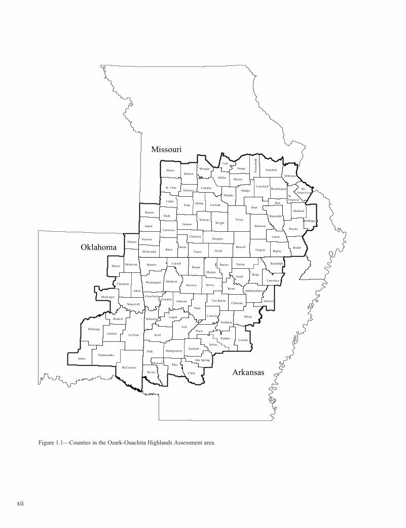
Figure 1.1—Counties in the Ozark-Ouachita Highlands Assessment area.
xii

Chapter 1: Major Air Pollutants
Question 1: What are the major emissionscharacteristics in the Ozark-Ouachita HighlandsAssessment area, and what areas receive thegreatest exposure to pollutants?
Air Quality in the Assessment Area
The term “air pollution” calls up images of dark fumesbillowing from tailpipes, black smoke from factorychimney stacks, or smog hanging over a city. Americansdepend on the combustion of fossil fuels for transporta-tion, electricity, industrial processes, and heating homesand businesses. This combustion of fossil fuels not onlygenerates energy, it also creates toxic gases and particu-lates. These pollutants can be transformed in the atmo-sphere and transported throughout the area of origin andbeyond. People and resources in the Ozark-OuachitaHighlands Assessment area (fig. 1.1) cannot escape airpollution and its effects.
Rarely can air pollution impacts be traced back to asingle source. Moreover, pollutants are generated fromboth within and outside of the Assessment area—evenfrom hundreds of miles away. Air pollution is producedby both human and natural activities and has three majorsources: (1) stationary or point sources such as power-generating plants, service stations and industrial facilities;(2) area sources such as dust from roads and smokefrom fires; and (3) mobile sources such as automobiles,trucks, and aircraft. The primary pollutants (such assulfur dioxide or nitrogen oxides) emitted directly fromthese sources are transformed in the atmosphere intosecondary pollutants such as sulfate or nitrates. In thisreport, the secondary pollutants discussed are those thatmost likely affect the forest environment.
The information presented in the following sections isfor a broad-scale assessment that focuses on air qualityissues concerning potential impacts to forest ecosystems.The information and data presented should be used
cautiously and may not be appropriate for local planning;that is, a statement that in general holds true for thewhole Ozark-Ouachita Highlands may not hold true for aspecific site in the Assessment area.
Primary Pollutants
Natural events such as dust storms, lightning-causedwildfires, and volcanoes release pollutants into theatmosphere as do human activities (also called anthropo-genic sources) such as agriculture, industry, transporta-tion, and prescribed fires.
In their analysis, the Atmospheric Team identified fourprimary pollutants released from human activities thateventually affect the Assessment area: particulate matter(10 microns and smaller, called PM10), nitrogen oxides,volatile organic compounds, and sulfur dioxide. Thesepollutants represent some of the six “Criteria Pollutants”recognized by the U.S. Environmental Protection Agency(EPA) (U.S. EPA 1995). The team selected these primarypollutants because secondary pollutants formed fromthem are suspected of causing visibility reductions andimpacts to vegetation and aquatic ecosystems. Informa-tion presented on these primary pollutants includes thelocation and intensity of emissions and likely future trendsin emissions.
Regional climate change resulting from emissions ofcarbon dioxide and other greenhouse gases is not dis-cussed in this report. Although the team recognized thatresources in the Ozark-Ouachita Highlands could besusceptible to climatic change, uncertainty concerning thenature of regional climatic changes and the global aspectsof the phenomenon led the team to conclude that acomprehensive analysis of this issue was beyond thescope of this Assessment. However, an overview of thebaseline climatic characteristics in the Assessment areacan be found in the “Climate” section of Chapter 1 of theOzark-Ouachita Highlands Assessment: AquaticConditions (USDA FS 1999).

Key Findings
1. The major types of air-pollution emissions with thepotential to impact the natural resources of theOzark-Ouachita Highlands are particulate matter,nitrogen oxides, volatile organic compounds, andsulfur dioxide.
2. Emissions of particulate matter are greatest alongthe northern and western boundaries of the Assess-ment area, where they are usually generated byfugitive dust sources (e.g., sources of uncontrolleddust emissions such as dirt roads or agriculturefields). Emissions in the future are expected toremain constant unless wildland or prescribed firesincrease beyond the current normal occurrences.
3. Nationally, motor vehicles and electrical utilities arethe usual sources of nitrogen oxides; however, in theAssessment area, fuel combustion at industrialsources is the major source of these emissions.Current measures taken by the U.S. EnvironmentalProtection Agency are likely to reduce emissions ofnitrogen oxides from electrical utilities and possiblyother sources.
4. Nationally and in the Ozark-Ouachita Highlands,motor vehicles are the main source of volatileorganic compounds caused by human activities.Available data were insufficient to enable theAtmospheric Team to project how volatile organiccompounds will change in the future.
5. Fuel combustion from electrical utilities is thegreatest source of sulfur dioxide in the Highlandsarea; the Atmospheric Team expects the amount ofemissions to decrease in the future due to theenactment of and full compliance with the Clean AirAct Amendments of 1990.
Data Sources and Methods of Analysis
States included in this analysis—Arkansas, Illinois,Kansas, Kentucky, Louisiana, Mississippi, Missouri,Nebraska, Oklahoma, Tennessee, and Texas—arelocated within 120 miles of the Ozark-Ouachita High-lands Assessment boundary. Table 1.1 lists the maincategories of emissions used in the analysis for thisAssessment (Miller 1997).
The Atmospheric Team obtained data from the EPAfor county-level estimates (tons/year) of emissions from
point and area sources for the 11 States. The team usedthe adjusted data from the EPA’s 1985 National AcidPrecipitation Assessment Program (NAPAP) inventory,using economic activity data to estimate the emissions for1994. The NAPAP inventory is organized by area andpoint source emission categories (Placet and others 1991).
The EPA also provided 1995 data on emissions ofnatural sources of nitrogen oxides and volatile organiccompounds for each county within the area (U.S. EPA1996). A simple rating system developed by the EPA(1996) was used to classify each county by the amount ofnatural or anthropogenic emissions recorded there. Theteam categorized each county by dividing the emissionsestimate for a pollutant by the area of the county, result-ing in “tons/square mile” (tons/mi2). They condensed thefive category system (table 1.2) used by the EPA (1996)into three categories: (1) low or below average, (2)average or above average, and (3) high. These categoriesallow comparisons of the emissions from a particularcounty with emissions from other areas in the UnitedStates. For example, a county with high emissions ofnitrogen oxides in the Assessment area would have more
2
Table 1.1—Main categories of area, mobile, andpoint source emissions in the Assessment area
Categorynumber Main category name
1 Fuel combustion, electrical utility 2 Fuel combustion, industrial 3 Fuel combustion, other 4 Chemical and allied product manufacturing 5 Metals processing 6 Petroleum and related industries 7 Other industrial processes 8 Solvent utilization 9 Residential wood and other10 Waste disposal and recycling11 Highway vehicles12 Off-highway vehicles13 Natural sources14 Miscellaneous15 Off-highway, other16 Agriculture and forestry17 Fugitive dust
Source: Miller (1997).

emissions per square mile than most counties in theUnited States.
It is difficult to define a specific boundary area for“contributing” sources because the atmospheric pro-cesses that control pollutant formation and transport varyby pollutant and as a function of weather conditions.Sources within the designated 120-mi radius and moredistant sources could contribute to pollutant levels.Atmospheric transport and dispersion models are tradi-tionally used to simulate pollution exposures across thelandscape or to map the potential downwind impact of apollution source. The most accepted regional models arevery expensive to use and were beyond the financialresources of this Assessment. Instead, a simplifiedapproach called statistical modeling was used for theanalysis. As shown in figure 1.2, the Atmospheric Teamlocated 28 receptors (spatial locations) over the Assess-ment area, using a 60-mi by 60-mi spacing. The teamselected a 120-mi radius to illustrate which sections of theOzark-Ouachita Highlands are likely to receive thegreatest pollution exposure. Only anthropogenic emissionswithin 120 mi of the receptors were used in the simplemodeling exercise.
The statistical model used for this Assessment is calledthe Pollution Exposure Index (PEI) (Miller 1997). Themodel has been developed using ArcView® software asan interface to perform the calculations. The team usedemissions from up to 405 counties in the analysis. Ifemissions from a county were less than 40 tons/year, theteam did not use them in the PEI model. Separate calcu-lations were performed for PM10, nitrogen oxides, sulfur
Table 1.2—Emissions categories described by the range of pollutants (tons per square mile)resulting from natural sources and human activities
Natural Human activity
Category NOx VOC PM10 NOx VOC SO2
- - - - - - - - - - - - - - - - - - - - - - - - - - Tons per square mile - - - - - - - - - - - - - - - - - - - - - - - - -
Low 0 – 0.20 0 – 2.0 0 – 6.9 0 – 1.13 0 – 1.21 0 – 0.07Below average 0.21– 0.30 2.1– 6.0 7.0 – 10.3 1.14 – 2.40 1.22– 2.61 0.08– 0.20Average 0.31– 0.60 6.1– 15.0 10.4 – 14.2 2.41 – 4.60 2.62– 4.76 0.21– 0.70Above average 0.61– 1.0 15.1– 25.0 14.3 – 19.7 4.61 –11.40 4.77–11.53 0.71– 4.80High > 1.0 > 25.0 > 19.7 > 11.40 >11.53 > 4.80
NOx = nitrogen oxides; VOC = volatile organic compounds; PM10 = particulate matter 10 microns or smaller; SO2 = sulfurdioxide.Source: U.S. EPA (1996).
dioxide, and volatile organic compounds. The model usedthe following equation:
PEIip = j
N
=∑
1
[(Fij * Tij) * Qjp / Dij]
and calculated a value for each of the 28 receptors. (Seethe sidebar for a complete explanation of the equationused.)
Figure 1.2—Location of receptors used for statisticalmodeling of pollution exposure within and near theAssessment area.
3

Patterns and Trends
Particulate Matter
Particulate matter in the atmosphere includes wind-blown soil, soot, smoke, and liquid droplets. It alsoincludes fine particles of sulfates, nitrates, and organiccompounds that are 2.5 microns or smaller in size(PM2.5). Particles are emitted into the air by sourcessuch as factories, power plants, construction activities,automobiles, fires, and agricultural activities. Relative tothe United States as a whole, many counties on thenorthern and western boundaries of the Assessment areahave high emissions of PM10 (fig. 1.3). Within the
The Atmospheric Team used the unpublished PEI model described by Miller (1997), which is as follows:
PEIip = j
N
=∑
1[(Fij * Tij) * Qjp / Dij]
where
PEIip = total index value for each receptor and pollutant of interest.i = receptors.p = pollutant of interest.N = total number of sources.j = source (i.e., the emissions from a county).Fij = annual wind direction percent frequency (using a 22.5 degree “window”), using the nearest surface wind station between the receptor and source.Tij = the calculated terrain factor between the receptor and the source (i.e., the county center).Qjp = pollutant emission rate (tons per year) for a particular pollutant.Dij = distance (kilometers) between the receptor and the source. Values less than or equal to 0.06 miles (0.1 km) were set to 0.06 miles (0.1 km).
The terrain factor (Tij) is an adjustment made if there are mountains between the receptor andsource. The calculation uses the following two equations:
Ee = max (Er, Es, Em)
Tij = Mh / Mh + (Ee - Es)where
Ee = largest value for Er, Es, or Em.Er = maximum receptor elevation (feet).Es = maximum source (i.e., county center) elevation (feet).Em = highest elevation (feet) along a line drawn between the source and the receptor.Mh = mixing height (average annual value of 2,689 feet was used).
The team then used the values at the receptors toestimate the PEI values between the receptors. SpatialAnalyst® (an ArcView® extension) was used to performthe estimates (also called interpolations). The team useda spline technique for the interpolations to a 6-mi by 6-migrid. The nearest 12 points to each grid were used for thespline interpolation. The results for the PEI model aregiven in tons per year per kilometer, which lacks meaningexcept as an index. Those areas with the highest valuesare believed to have the highest risk of impact from aparticular pollutant. The results from the PEI modelshould be used cautiously and in conjunction with avail-able ambient monitoring data.
4
5
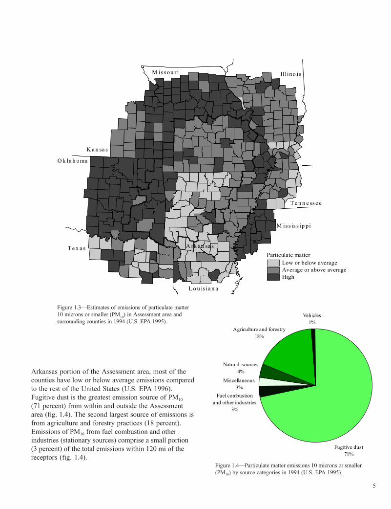
Figure 1.3—Estimates of emissions of particulate matter10 microns or smaller (PM
10) in Assessment area and
surrounding counties in 1994 (U.S. EPA 1995).
Figure 1.4—Particulate matter emissions 10 microns or smaller(PM10) by source categories in 1994 (U.S. EPA 1995).
Natural sources4%
Vehicles1%
Agriculture and forestry18%
Fugitive dust71%
Miscellaneous3%
Fuel combustion and other industries
3%
Arkansas portion of the Assessment area, most of thecounties have low or below average emissions comparedto the rest of the United States (U.S. EPA 1996).Fugitive dust is the greatest emission source of PM10
(71 percent) from within and outside the Assessmentarea (fig. 1.4). The second largest source of emissions isfrom agriculture and forestry practices (18 percent).Emissions of PM10 from fuel combustion and otherindustries (stationary sources) comprise a small portion(3 percent) of the total emissions within 120 mi of thereceptors (fig. 1.4).

Vehicles22%
Other industries7%
Fuel combustion, industrial
28%
Fuel combustion, other9%
Fuel combustion, electrical utilities
20%
Miscellaneous 14%
Nitrogen Oxides
More than 95 percent of nitrogen oxide emissions is inthe form of nitric oxide. In the presence of volatileorganic compounds and sunlight, this gas is rapidlyconverted in the atmosphere to nitrogen dioxide, whichcan subsequently be altered by sunlight to produce ozone.Available evidence suggests that nitrogen oxides are acontrolling factor in the formation of ground-level ozonein rural areas of the Southern United States (Chameidesand Cowling 1995). When trapped in sufficient quantities,nitrogen dioxide can be seen as a brownish haze. Second-ary pollutants formed from nitrogen oxides also reducevisibility and contribute to acid deposition. The largestcontributors of nitrogen oxides within 120 mi of thereceptors (fig. 1.5) are fuel combustion from industrialsources (28 percent), motorized vehicles (22 percent),and electrical utilities (20 percent). Nationally, greaterportions of total nitrogen oxide emissions come from
motorized vehicles (45 percent) and electrical utilities (33percent). On the other hand, national nitrogen oxideemissions from industrial fuel combustion comprise asmaller portion (14 percent) of the total than in theAssessment area (U.S. EPA 1995).
Figure 1.6 shows which counties have the largestreleases of nitrogen oxides from anthropogenic sources.The areas with high annual emissions correspond to thelarger cities within or outside the Assessment areaincluding Little Rock, AR; St. Louis, MO; Kansas City,MO; Tulsa, OK; and Dallas, TX. Within the Assessmentarea, most of the county-level emission estimates arelow or below average in comparison to other counties inthe United States. Figure 1.6 does not include emissionestimates of nitrogen oxides from natural sources. The1995 emissions from natural sources were low or belowaverage throughout most of the Assessment area(fig. 1.7).
Figure 1.5—Emissions of nitrogen oxide (NOx) by source categories, based on1994 data (U.S. EPA 1995).
6

Figure 1.6—Estimates of human-caused nitrogenoxide (NOx) emissions in Assessment area andsurrounding counties in 1994 (U.S. EPA 1995).
Figure 1.7—Estimates of natural nitrogen oxide (NOx) emissions inAssessment area counties in 1995.
7

Volatile Organic Compounds
Volatile organic compounds represent a wide range oforganic chemicals that are emitted into the atmosphere.Combined with nitrogen dioxide, these chemicals contrib-ute to the formation of ground-level ozone. Trees are theprimary source of naturally produced volatile organiccompounds (Placet and others 1991), and much of theAssessment area is forested and has high natural emis-sions (see fig. 1.8) compared to other counties in theUnited States. As in the rest of the Nation, motor vehicleuse is the main human (anthropogenic) source of volatileorganic compounds, accounting for 37 percent of the totalemissions (U.S. EPA 1995) (fig. 1.9). Solvent utilization(27 percent) and processes at petroleum and relatedindustries (14 percent) also release volatile organiccompounds within 120 mi of the receptors. Figure 1.10shows a wide range of anthropogenic emissions fromcounties within 120 mi of the receptors; the highestemissions of volatile organic compounds occur near citiessuch as Dallas, TX; St. Louis, MO; and Memphis, TN.
Vehicles37%
Solvent utilization27%
Petroleum and related industries
14%
Miscellaneous12%
Fuel combustion and other industries
10%
8
Figure 1.8—Estimates of natural volatile organic compoundemissions in Assessment area counties in 1995.
Figure 1.9—Sources of volatile organic compound emissions in 1994 (U.S.EPA 1995).

Figure 1.10—Estimates of human-caused volatile organic compound emissions in Assessment area and surround-ing counties in 1994 (U.S. EPA 1995).
9

Sulfur Dioxide
Sulfur dioxide is a gas transformed in the atmosphereinto secondary pollutants called sulfates, the main con-tributors to visibility reduction and acid deposition. Electri-cal utilities are the largest source of sulfur dioxideaffecting the Highlands (72 percent) (fig. 1.11), which isconsistent with the national pattern (U.S. EPA 1995).There are very few emissions of sulfur dioxide fromnatural sources in the Assessment area. As with nitrogenoxides or volatile organic compounds, the counties withthe largest emissions are near the largest cities (fig. 1.12).
Vehicles1%
Fuel combustion, electrical utilities
72%
Fuel combustion, industrial
15%
Other industries and miscellaneous
11%
Fuel combustion, other1%
10
Figure 1.11—Sources of sulfur dioxide (SO2) emissions in1994 (U.S. EPA 1995).
Figure 1.12—Estimates of human-caused sulfur dioxide (SO2) emissions in Assessment area and surrounding counties in1994 (U.S. EPA 1995).
Fuel combustion,electrical utilities
72%
Vehicles1%
Other industries andmiscellaneous
11%
Fuel combustion, other1%
Fuel combustion,industrial
15%

Pollution Exposure Index Results
The Atmospheric Team used two approaches toidentify which areas receive the greatest exposure topollutants: (1) ambient monitoring data and (2) a statisticalapproach. The team found that there were few ambientmonitoring sites across the Assessment area, which is thecase in rural areas such as the Ozark-Ouachita High-lands. With little data, it is difficult to interpret pollutionpatterns, so the team chose an additional approach. Theyconsidered using an atmospheric dispersion model topredict the transformation of primary pollutants (such assulfur dioxide) and where the secondary pollutants (suchas sulfates) are likely to be the greatest. There arenumerous complex atmospheric models available, but thecost was prohibitive. Therefore, the Atmospheric Teamchose to use the statistical PEI model (Miller 1997),described earlier, to identify areas with the greatestpollution exposure.
The PEI values are calculated based upon: (1) theannual emission of the specific pollutant, (2) the distancebetween the source and receptor, (3) the frequency ofwinds blowing from the source toward the receptor(assuming a straight-line windflow), and (4) the degree towhich hills or mountains impede the windflow. The resultsfrom the PEI model do not predict pollutant deposition ofsecondary pollutants (such as sulfates or ozone). There-fore, the model results should not be used to say thatimpacts are occurring from a specific pollutant. Further-more, the PEI uses the direction frequency of groundlevel winds, which is usually not reliable at locations farfrom a measurement site. Atmospheric dispersion modelsuse the results of complex meteorology modeling toestimate wind directions and speeds at ground level andvarious heights in the atmosphere. The PEI model doesnot take into account local topographic effects on windfields; therefore, a person must be cautious when makingany strong statements about a specific spot in the As-sessment area. The model is useful because it predictswhich portions of the region are most likely to have thegreatest pollution exposure from anthropogenic sources,and it may be useful in locating where further monitoringshould be conducted.
As has been noted, the greatest source of PM10
emissions is fugitive dust (fig. 1.4) in the western andnorthern counties within the Assessment area (fig. 1.3).Therefore, the PEI model predicts that PM10 exposures
are likely to be greatest along the western portions of theAssessment area (fig. 1.13). PM10 exposures in the airare likely to be less in the central portions of the Assess-ment area because particles transported eastward bypredominately westerly winds are likely to deposit fromthe atmosphere near their sources (fig. 1.13).
The team did not have emission estimates from naturalsources of volatile organic compounds and nitrogenoxides within 120 mi of the receptors (fig. 1.2). There-fore, only anthropogenic emission estimates for volatileorganic compounds and nitrogen oxides were used asinput into the PEI model. Assessing where these pollut-ants have the potential for the greatest impact is difficultsince the PEI model does not include transformation ofthese emissions to ground-level ozone or nitrate deposi-tion. The PEI results for nitrogen oxides and volatileorganic compounds are shown in figures 1.14 and 1.15,respectively. The model simulations suggest that anthro-pogenic exposure to nitrogen oxides and volatile organiccompounds is lowest in the interior and highest near theperimeter of the Assessment area—particularly near theeast-central, west-central, and northeastern perimeters.
Figure 1.13—Pollution Exposure Index modeling resultsusing 1994 particulate matter (PM10) emissions data.
11

Chameides and Cowling (1995) suggest that ozoneformation is likely to be greater downwind of nitrogenoxide sources because volatile organic compoundstypically are not a limiting factor in rural areas of theSouthern United States. The PEI results for nitrogenoxides (fig. 1.14) suggest ozone exposures are likely tobe greatest in the Ozark-Ouachita Highlands downwindof St. Louis, MO; Little Rock, AR; Dallas, TX; andTulsa, OK.
The Atmospheric Team decided the PEI results shouldnot be used to predict where sulfate and nitrate depositionwould be the greatest because the total deposition in agiven area is the sum of the amount in the rainfall, dry fall(usually seen as haze), and cloud water. Furthermore, fineparticles (2.5 microns or smaller) of sulfates and nitratestravel very long distances before settling to the ground.The PEI results in figures 1.14 and 1.16 show wherenitrogen and sulfur (such as nitrogen oxide and sulfurdioxide) exposures may be the greatest. As mentionedpreviously, exposures to nitrogen oxide emissions may bethe greatest downwind of several large cities within ornear the Assessment area (fig. 1.14). Exposure to sulfurcompounds is likely to be greatest in the northeasternportion of the Assessment area near St. Louis, MO.
One consistent pattern from the PEI model results isevident (figs. 1.13 to 1.16). The modeling results of theemissions from the four primary pollutants of interestindicate a pattern throughout a large portion of theAssessment area that suggests that pollution exposuresshould be less there, whereas they appear to be higherclose to the boundary.
Emission Trends
The Clean Air Act (CAA) is the primary means bywhich the American public’s health and welfare (as theyrelate to air pollution) are protected. Implementation ofthe CAA and its amendments since 1977 has resulted insignificant reductions for several primary pollutants (fig.1.17). Nationally, particulate matter emissions fromstationary sources decreased significantly between 1940and 1994 (fig. 1.17), but total PM10 emissions have notdecreased because a large portion is from fugitive dustsources (U.S. EPA 1995). Therefore, total PM10 emis-sions are predicted to remain constant in the futurebecause there are no initiatives that would significantlyreduce fugitive dust emission.
Figure 1.14—Pollution Exposure Index modeling resultsusing 1994 human-caused nitrogen oxide (NOx)emissions data.
Figure 1.15—Pollution Exposure Index modeling resultsusing 1994 human-caused volatile organic compoundemissions data.
12
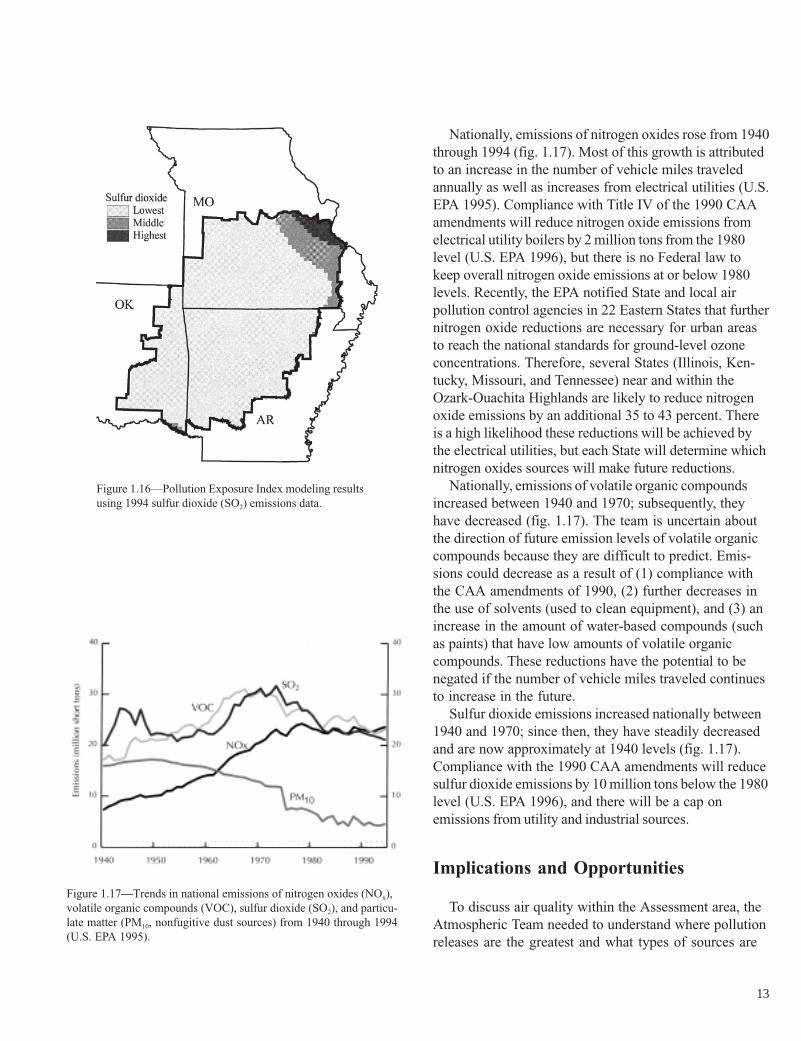
Figure 1.16—Pollution Exposure Index modeling resultsusing 1994 sulfur dioxide (SO2) emissions data.
Figure 1.17—Trends in national emissions of nitrogen oxides (NOx),volatile organic compounds (VOC), sulfur dioxide (SO2), and particu-late matter (PM10, nonfugitive dust sources) from 1940 through 1994(U.S. EPA 1995).
Nationally, emissions of nitrogen oxides rose from 1940through 1994 (fig. 1.17). Most of this growth is attributedto an increase in the number of vehicle miles traveledannually as well as increases from electrical utilities (U.S.EPA 1995). Compliance with Title IV of the 1990 CAAamendments will reduce nitrogen oxide emissions fromelectrical utility boilers by 2 million tons from the 1980level (U.S. EPA 1996), but there is no Federal law tokeep overall nitrogen oxide emissions at or below 1980levels. Recently, the EPA notified State and local airpollution control agencies in 22 Eastern States that furthernitrogen oxide reductions are necessary for urban areasto reach the national standards for ground-level ozoneconcentrations. Therefore, several States (Illinois, Ken-tucky, Missouri, and Tennessee) near and within theOzark-Ouachita Highlands are likely to reduce nitrogenoxide emissions by an additional 35 to 43 percent. Thereis a high likelihood these reductions will be achieved bythe electrical utilities, but each State will determine whichnitrogen oxides sources will make future reductions.
Nationally, emissions of volatile organic compoundsincreased between 1940 and 1970; subsequently, theyhave decreased (fig. 1.17). The team is uncertain aboutthe direction of future emission levels of volatile organiccompounds because they are difficult to predict. Emis-sions could decrease as a result of (1) compliance withthe CAA amendments of 1990, (2) further decreases inthe use of solvents (used to clean equipment), and (3) anincrease in the amount of water-based compounds (suchas paints) that have low amounts of volatile organiccompounds. These reductions have the potential to benegated if the number of vehicle miles traveled continuesto increase in the future.
Sulfur dioxide emissions increased nationally between1940 and 1970; since then, they have steadily decreasedand are now approximately at 1940 levels (fig. 1.17).Compliance with the 1990 CAA amendments will reducesulfur dioxide emissions by 10 million tons below the 1980level (U.S. EPA 1996), and there will be a cap onemissions from utility and industrial sources.
Implications and Opportunities
To discuss air quality within the Assessment area, theAtmospheric Team needed to understand where pollutionreleases are the greatest and what types of sources are
13

emitting specific pollutants. The team compiled county-level data that can be used by land managers and othersto see how a proposed action (e.g., a community in theAssessment area is looking for a new industry or pre-scribed fire is needed to reduce undergrowth) mayinfluence emissions from a specific county. Emissionsestimates are critical for such determinations. Futureassessments should gather emission estimates for the
primary pollutants considered in this report, as well asparticulate matter 2.5 microns and smaller (PM2.5) in size.Also, further work after this Assessment, or a futureassessment, could use one or more complex atmosphericdispersion models to gain a more complete understandingof how the emissions from an area will impact a down-wind region.
14

Chapter 2: Particulate Matter (PM10) in the Air
Question 2: What is the status of particulatematter in the Ozark-Ouachita Highlands?
The previous chapter provided a description of someof the relevant pollutant emissions characteristics withinthe Assessment area, including particulate matter. Thischapter provides a more indepth analysis of the typicalseasonal particulate matter concentration patterns in theatmosphere over the Assessment area that result fromthe emissions patterns described in Chapter 1.
Particulate matter (PM10) as an air pollutant consistsof those particles suspended in the atmosphere that are10 microns or smaller in diameter. The most importantconstituents of particulate matter are particles 2.5microns in diameter (PM2.5) or smaller. These tinyparticles can be breathed into human lungs and createserious health problems (e.g., respiratory ailments andasthma). White (1995) of the American Lung Associa-tion maintains that there is no tolerance level belowwhich particulates do not affect human health. Statedanother way—any increase in particulate concentration
can cause an increase in human health problems. Theseproblems have been triggered at concentrations wellbelow current National Ambient Air Quality Standards(NAAQS) (White 1995).
Particulates come from many sources: industry,electrical power production, internal combustion engineexhaust, dust from natural and artificial sources, smokefrom agricultural and forestry burning, and wildland fires.The U.S. Environmental Protection Agency (EPA)categorizes sources of particulate matter emissions thatare 10 microns or smaller in diameter (PM10) as pointsources (smokestack emissions) or fugitive processsources (e.g., dust, leaks, uncontrolled vents). Fugitivedust is also generated by wind erosion, agricultural tilling,mining, construction, and both paved and unimprovedroads (U.S. EPA 1996).
Even though industrial production has increasednationally during recent decades, pollution control equip-ment has dramatically reduced PM10 emissions fromindustrial processes (fig. 1.17). Figure 2.1 illustrates thatin 1970, smokestacks generated over 12 million tons ofPM10 particles, while in 1995, they produced only about2.5 million tons (U.S. EPA 1996). The Clean Air Act
Figure 2.1—National smokestack and miscellaneous particulate matter (PM10) emissions(in million short tons) from 1970 through 1995 (U.S. EPA 1996).
15

(1970) and its amendments (1977 and 1990) encouragedthis abatement.
According to the guidelines of the NAAQS, PM10
concentrations at any location are not to exceed 150micrograms per cubic meter (µg m-3) during a 24-hourperiod. The NAAQS also limit the average annualexposure of PM10 at any location to 50 µg m-3. In July1997, the EPA implemented a new ambient air qualitystandard based on particulate matter 2.5 microns orsmaller in diameter (PM2.5). This new standard statesthat the average annual and 24-hour concentrations arenot to exceed 15 µg m-3 and 65 µg m-3, respectively, atmonitoring sites that represent a large-scale area and arenot related to a specific source.
In addition to its potential effect on human health,particulate matter reduces visibility (discussed in the nextchapter). Within the Assessment area, all areas presentlymeet the PM10 NAAQS. There are no chronic particu-late matter (PM) problems on or near national forestlands in Arkansas or Oklahoma. In southern Missouri,however, the charcoal industry has created a locality withreoccurring days of high PM concentrations (Braun1996). The State is looking into this situation.
Key Findings
1. Particulate matter concentrations (PM10) show adefinite seasonal trend over the Assessment area.The highest concentrations between 1991 and 1995were during the summer months, with an averageperiod concentration of 33.05 micrograms per cubicmeter (µg m-3); the average winter concentrationwas 19.84 µg m-3.
2. Rural areas have lower PM10 concentrations thanurban areas.
3. There is a spatial distribution of PM10 across theAssessment area, with the lowest annual averagePM10 concentrations occurring in western Arkansas.
4. The Assessment area is well within the NationalAmbient Air Quality Standards (NAAQS) for PM10.Implementation of the new PM2.5 regulations maycreate a challenge to prescribed burning programs offarmers and land management agencies such as theUSDA Forest Service.
Data Sources and Methods of Analysis
Most data analyzed for this Assessment are from theEPA’s Aerometric Information Retrieval System (AIRS).In addition, the team used data from the InteragencyMonitoring of Protected Visual Environment (IMPROVE)monitoring network.
The AIRS data base is the national data storagesystem for all Criteria Pollutants. Data were obtainedfrom AIRS sites both inside and within 100 miles (mi) ofthe Assessment area boundary. The EPA sets rigid datacollection standards and assures the quality of all dataentered into the system. Because the EPA changed PMstandards in 1987 from measurement of total suspendedparticles (TSP) to PM10, the team decided to avoid usingTSP data and instead chose PM10 data from 1991 to1995 because all sites were monitoring with PM10
equipment by 1991. The point data were displayed usingthe Geographic Information System (GIS) softwarecalled ArcInfo®. These data were analyzed across theAssessment area using the “inverse distance weightingmethod” (Burrough 1988) and then displayed in a gridformat. Each grid was assigned a value. These gridvalues represent estimated rather than measured values.This limitation needs to be considered when makingassertions or recommendations using these or similardata.
16
Patterns and Trends
Table 2.1 shows the seasonal, annual, and periodmeans of PM10 concentrations over the entire Assess-ment area based on observational data from the AIRSnetwork (mainly urban areas). The numbers in table 2.1represent averages of all the PM10 monitors inside theAssessment area from 1991 through 1995. The seasonal-ity of PM10 is clearly evident in table 2.1, with theaverage PM10 concentrations at AIRS monitoring sitesover the entire Assessment area typically increasing fromwintertime minimum values to summertime maximumvalues. Figure 2.2 shows the typical, large-scale spatialdistributions of PM10 concentrations for each season overthe Assessment area based solely on AIRS networkdata. Because most observation sites in the AIRSnetwork are in urban areas where PM10 concentrationstend to be higher than in rural settings, the interpolatedspatial patterns of PM10 concentrations across theAssessment area most likely overestimate nonurbanPM10 concentrations. Nevertheless, the spatial patternsshown in figure 2.2 provide a general indication of theimpact of urban PM10 emission sites on PM10 concentra-tions in the Assessment area.
The interpolated mean winter PM10 data from theAIRS network shown in figure 2.2 indicate that mostPM10 concentrations in the Assessment area are lessthan 22.5 µg m-3 (based on 1991 to 1995 data). Concen-trations tend to increase during the spring months overparts of the Assessment area, particularly over thewestern and eastern sections of the Assessment area aswell as in southern Missouri (fig. 2.2). The interpolated
Table 2.1—Average PM10 concentrations (in µg m-3) in theAssessment area by season, year, and 5-year period
1991–Season 1991 1992 1993 1994 1995 1995
Winter 21.68 21.04 19.47 19.74 18.33 19.84Spring 23.75 25.05 22.32 25.53 24.69 24.08Summer 34.04 31.29 34.12 25.47 32.81 33.05Fall 26.74 23.52 21.61 23.59 28.09 24.77Annual 26.35 25.20 24.29 25.43 25.93 25.47
PM10 = particulate matter 10 microns or smaller; µg m-3 = microgramsper cubic meter.
AIRS PM10 data indicate average spring concentrationsin these regions are about 22.51 to 27.5 µg m-3, althoughactual mean concentrations in some of the more rurallocations in these regions are probably less. In centralArkansas, average springtime concentrations are gener-ally lower. The highest particulate matter concentrationsthroughout the Assessment area are usually found duringthe summer months (fig. 2.2). The interpolated AIRSdata suggest summertime PM10 concentrations in theAssessment area often exceed 27.5 µg m-3 (especially inurban areas). Particulate matter concentrations tend todecrease during the fall months, although they are stillrelatively high compared to the wintertime minimumconcentrations (fig. 2.2). The far northern sections of theAssessment area experience the most dramatic decreasein PM10 concentrations from the summer to fall seasons.Based solely on AIRS network data, the annual meanPM10 concentrations for the entire period over most ofthe Assessment area range from 22.51 to 27.5 µg m-3
(fig. 2.3), well within the present NAAQS of 50 µg m-3.The seasonality of PM10 is partly due to increased dust
production in the spring and summer months compared tothe winter months—especially during dry years—as wellas increased power production for air conditioning. Also,emissions from automobiles and other internal combustionengines increase during the summer. Another source ofparticulate matter is the natural increase in atmosphericmoisture (water vapor) during the summer. Certain kindsof particles, especially sulfates, are hygroscopic (meaningthey attract water), which increases their weight. TheAIRS data also appear to indicate the effects of agricul-tural tillage. For example, in March, higher PM10 valuesshow up in southwestern Missouri during tillage; in Apriland May, these higher concentrations are in the agricul-tural areas in Arkansas (tillage occurs later because thearea retains wetness). (Monthly maps are available uponrequest from the Forest Service in Arkansas—seeinformation inside the front cover of this report.)
Figure 2.4 illustrates the average PM10 mass concen-trations in µg m-3 from 1992 to 1995 at sites in theIMPROVE network. These are Class I wildernessareas—wildernesses that are larger than 5,000 acres andnational parks larger than 6,000 acres in existence on orbefore August 7, 1977. Class I areas are defined by theClean Air Act (CAA) amendments of 1977 as having“special protection” from effects of air pollution because
17

Figure 2.2—Average PM10 values (µg m-3) during winter, spring, summer, and fall from 1991 through 1995.
18

Figure 2.3—Average PM10 values (µg m-3) for the 1991 through 1995 period.
of their “air-quality related values (AQRV’s),” i.e., waterquality, native vegetation, ecosystem integrity, andvisibility. Figure 2.4 indicates that the annual mean PM10
concentrations in the Class I areas within the Assessmentarea are between 15 and 18 µg m-3 (average concentra-tion at Deer, AR—a nonurban area—is 17.4 µg m-3).Comparing these values with the annual mean PM10
concentration in urban areas (AIRS network data) withinthe Assessment area (25.47 µg m-3 from table 2.1)suggests that the rural forested regions in the Assessmentarea have about 30 to 40 percent less particulate matterthan the urban areas when averaged over an entire year.
Prescribed burning is currently a minor source ofparticulate emissions in the Highlands area on a yearlybasis. The 1995 level of managed burning reported by theEPA produced 538 short tons of emissions, accountingfor 1.3 percent of the national total PM10 emissions (U.S.EPA 1996). These emissions include silvicultural andagricultural burning. On shorter time scales, however,prescribed burning can result in significant local emissionsof particulate matter. Two studies have been reported inthe Southern States where portable PM10 monitors wereset up adjacent to prescribed fires for 2 to 12 hours. TheFlorida Department of Environmental Protection and the
19
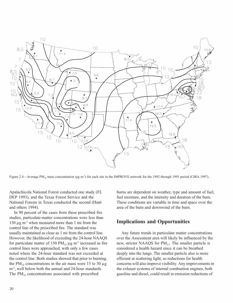
Figure 2.4—Average PM10 mass concentration (µg m-3) for each site in the IMPROVE network for the 1992 through 1995 period (CIRA 1997).
Apalachicola National Forest conducted one study (FLDEP 1993), and the Texas Forest Service and theNational Forests in Texas conducted the second (Huntand others 1994).
In 90 percent of the cases from these prescribed firestudies, particulate-matter concentrations were less than150 µg m-3 when measured more than 1 mi from thecontrol line of the prescribed fire. The standard wasusually maintained as close as 1 mi from the control line.However, the likelihood of exceeding the 24-hour NAAQSfor particulate matter of 150 PM10 µg m-3 increased as firecontrol lines were approached, with only a few casesnoted where the 24-hour standard was not exceeded atthe control line. Both studies showed that prior to burning,the PM10 concentrations in the air mass were 15 to 30 µgm-3, well below both the annual and 24-hour standards.The PM10 concentrations associated with prescribed
burns are dependent on weather, type and amount of fuel,fuel moisture, and the intensity and duration of the burn.These conditions are variable in time and space over thearea of the burn and downwind of the burn.
Implications and Opportunities
Any future trends in particulate matter concentrationsover the Assessment area will likely be influenced by thenew, stricter NAAQS for PM2.5. The smaller particle isconsidered a health hazard since it can be breatheddeeply into the lungs. The smaller particle also is moreefficient at scattering light, so reductions for healthconcerns will also improve visibility. Any improvements inthe exhaust systems of internal combustion engines, bothgasoline and diesel, could result in emission reductions of
20

particulate matter. Also, dust abatement on gravel roadsmay become necessary in some areas. Until the PM2.5
monitoring system mandated by the new NAAQSprovides the data, the impact of the stricter standards onthe use of prescribed fire will remain conjecture. It will beapproximately 5 years before these data will be available.
How will the new PM2.5 regulations impact the use ofprescribed fire? Haddow (1990) found that approxi-mately 70 percent of the particulate matter produced bywildland fuels is within the PM2.5 size class. The pro-posed regulations call for the 24-hour standard to be lessthan 65 µg m-3 and the annual average to be less than15 µg m-3. Figure 2.5 illustrates that the 1992 to 1995annual average concentration of fine mass particles(diameter of 2.5 microns or smaller) was between 9 and11 µg m-3 over the more rural areas of the Assessment
area based on interpolated IMPROVE network data.These concentrations represent between 60 and 73percent of the proposed standard annual average of15 µg m-3 and 18 to 22 percent of the current annualstandard of 50 µg m-3. Thus, even with the implementa-tion of the new PM2.5 standards, the more rural sectionsof the Assessment area should still be in compliance ifcurrent PM2.5 concentration averages continue tocharacterize the region.
According to Forest Service records, most prescribedburning occurs during March in the Assessment area.Average PM10 concentrations in the Assessment areaduring March (from 1991 through 1995)—when pre-scribed burning is common—ranged from a minimumof 10 to 20 µg m-3 to a maximum of 30 to 40 µg m-3
(fig. 2.6) with a mean of 22.7 µg m-3 (based on
Figure 2.5—Average fine particle mass (PM2.5) concentrations (µg m-3) for each site in the IMPROVE network for the 1992 through 1995 period(CIRA 1997).
21

interpolated AIRS data). If prescribed fire becomes amore widely used land management tool in the Assess-ment area during the normal prescribed fire season, totalPM10 and PM2.5 emissions and concentrations in the
Figure 2.6—Average PM10 concentrations (µg m-3) during March for the 1991 through 1995 period.
atmosphere will likely increase during the springtime.These increases would lead to a more dramatic degra-dation of air quality from the winter to spring seasonsthan what is currently observed (fig. 2.2).
22
Chapter 3: Visibility
Question 3: How good is visibility in theAssessment area; how does air pollution affectvisibility?
The Ozark-Ouachita Highlands are blessed withscenic beauty. Visitors and residents want to be able toenjoy the natural sights surrounding them. In fact, one ofthe reasons most often given for living near or visiting theHighlands is to enjoy the scenery. The clarity of air—orvisibility—affects the ability to see the pine and oakcovered mountains, rocky bluffs, and scenic streams ofthe Highlands. In addition to being an important compo-nent of the quality of life in the region and a major factorin recreation and tourism, visibility is protected by Federallaw. The Clean Air Act (CAA) amendments of 1977declared “ . . . as a national goal the prevention of anyfuture, and the remedying of any existing, impairment ofvisibility in mandatory Class I Federal areas . . .” whensuch an impairment results from air pollution caused byhuman activities. Within the Highlands, there are threeClass I areas: Caney Creek Wilderness on the OuachitaNational Forest, Upper Buffalo Wilderness on the Ozark-St. Francis National Forests, and Hercules Glade Wilder-ness on the Mark Twain National Forest. (MingoWilderness, a Class I area managed by the U.S. Fish andWildlife Service, lies near the eastern border of theMissouri Ozarks.)
Visibility impairment is most simply described as thehaze that obscures clarity, color, texture, and form.Several components interact to determine visibilityconditions: (1) the object being viewed, (2) atmosphericconditions influencing the sight path, (3) lighting condi-tions, and (4) the viewer. Visibility impairment is causedby aerosols (solid or liquid particles dispersed in the air)or gases in the atmosphere that scatter or absorb light.Knowledge of the chemical and physical properties of the
aerosols responsible for visibility impairment can provideinsight into the causes of visibility problems. Scatteringefficiency for visible light is greatest for particles andaerosols with diameters in the 0.1 to 1.0 micron range.Fine particles with diameters of 2.5 microns or smaller(PM2.5) contribute greatly to the scattering and absorptionof light, the sum of which is called light extinction. Thesignificant chemical components in fine aerosols aresulfates, nitrates, organic carbon, soot (light-absorbingcarbon), and soil dust.
A wide variety of pollutants may result from dailyactivities that include driving cars, generating electricity,and producing consumer goods. Depending on location,time of year, and atmospheric conditions, these pollutantscan significantly reduce visibility.
Once pollutants enter the atmosphere, their fate islargely determined by meteorological conditions, espe-cially winds, relative humidity, and solar radiation.According to the U.S. Environmental Protection Agency(EPA) (1995), most visibility impairment results from thetransport by winds of emitted aerosols, often over greatdistances (typically hundreds of miles). Consequently,visibility impairment is usually a regional problem ratherthan a local one. Regional haze is caused by the com-bined effects of emissions from many sources distributedover a large area, rather than from individual plumescaused by a few sources at specific sites. Stable atmo-spheric conditions produce stagnation areas that inhibitmovement of pollutants, sometimes leading to severehaze episodes (Holzworth and Fisher 1979).
Relative humidity is another weather parameter thataffects visibility. In a humid atmosphere, sulfate particlescombine with water and grow to sizes that make themmore efficient light scatterers. Thus, for a given level ofpollution, an atmosphere with higher relative humidity willhave more haze than one with lower relative humidity(Sisler and others 1993).
23

Key Findings
1. A definite seasonal pattern exists. The best visibilityoccurs during the fall, and the worst visibility occursduring the summer. Summer is also the time ofhighest PM2.5 concentrations.
2. The Upper Buffalo Wilderness on the Ozark-St.Francis National Forests has the best visibility of thethree Class I wilderness areas on national forestswithin the Assessment area.
3. Sulfates are the primary aerosols responsible forvisibility impairment within the Assessment area.
4. Visibility impairment in the form of regional hazeexists within the Assessment area, but the teamfound that there are not enough data to identifytrends.
5. Compliance with the Clean Air Act amendments of1990 should reduce sulfates and improve visibility.
Data Sources and Methods of Analysis
Scientists and resource managers use several differenttypes of equipment to measure visibility conditions, eachof which differs in terms of cost, siting restrictions, easeof operation, and usefulness of data. The most commontypes of optical visibility-monitoring equipment include thetransmissometer and the nephelometer. These toolsdirectly measure the light-extinction coefficient andscattering coefficient, respectively. Scenic monitoringuses interpretation of 35-mm photographic slides. Aerosolmonitors measure the particles in the atmosphere thataffect visibility. Combinations of these types of equipmentare used to describe and define visibility.
Three different parameters are used to expressvisibility: standard visual range (SVR), light extinctioncoefficient (Bext), and the deciview (dv). The ForestService commonly uses the SVR derived from photo-graphs to measure visibility, although this method has afair amount of uncertainty associated with it because ofthe subjective nature of estimates from photographs. TheSVR, usually expressed in kilometers, is the greatestdistance at which an observer can barely see a black
object the size of a mountain viewed against the horizonsky. The higher the SVR value, the better the visibility.
Another common measure of visibility is the Bext,which represents the ability of the atmosphere to absorband scatter light. As the light-extinction coefficientincreases, visibility decreases. Direct relationships existbetween concentrations of particles in the air and theircontribution to the extinction coefficient. These relation-ships are often presented in an annual extinction-budgetplot showing the percentage of light extinction attributedto each particle type. The extinction budget (discussedfurther later) is an important method for assessing thecauses of visibility impairment.
Neither the SVR nor the Bext has a consistent directrelationship to perceived visual changes caused by uniformhaze. Depending on baseline visibility conditions, a specificchange in the SVR or the Bext can result in a visualchange that is either obvious or imperceptible relative tothe total SVR. For example, an improvement of 10 miles(mi) in SVR may be quite perceptible at an easternlocation with an annual average visibility of 40 mi, but a10-mi change in SVR may not be perceptible at a west-ern location with an annual average visibility of 150 mi.
The dv is another commonly used measure of visibility(Pitchford and Malm 1994). The dv is designed to beperceptually linear (similar to the decibel scale for sound),meaning that a change of any given dv should appear tohave approximately the same magnitude of visual changeon any scene regardless of baseline visibility conditions.(The dv is designed to describe changes in visibilityperception across locations with all types of baselineconditions.) A change of 1 dv is about a 10 percentchange in the Bext—a small but perceptible change invisibility. The dv value increases as haze increases, so itis known as a haziness index.
The Forest Service has collected visibility data withcameras at the three Class I areas within the Assessmentarea, and Air Resource Specialists, Inc., of Fort Collins,CO, has analyzed the findings. Fine mass data (PM2.5)were collected as part of the IMPROVE network (Sislerand others 1996). These data were then used to deter-mine extinction budgets showing the percentage of eachdifferent aerosol pollutant that causes visibility degrada-tion measured in terms of the SVR.
24

Patterns and Trends
Table 3.1 gives the average annual camera-basedSVR in miles and kilometers as well as the haze factor indv’s for the Class I wilderness areas of the Assessmentarea from 1988 to 1995. Estimates in this table indicatethat Upper Buffalo has the best visibility—perhapsbecause of the remoteness of this wilderness and prevail-ing precipitation patterns. Caney Creek normally receivesmore precipitation than Upper Buffalo and HerculesGlade. The resultant greater number of foggy days andhigher relative humidity at Caney Creek would accountfor the reduced visibility. Photographs of the visibilityconditions at the three Class I wildernesses can be seenin figures 3.1 to 3.3.
Figures 3.4 and 3.5 represent the average “clear day,”“median day,” and “hazy day” fine particle (PM2.5)budgets at the Upper Buffalo IMPROVE site for the fourseasons from 1992 through 1995. The “fine mass budget”pie charts show the actual percentages of the particlecomponents, based on weight. The “extinction budget”pie charts show by what percentage each constituentreduces visibility.
The top half of figure 3.4 shows that during the wintermonths over this time period, PM2.5 concentrations at theUpper Buffalo site averaged 3.5 milligrams per cubicmeter (µg m-3) on “clear days,” 6.7 µg m-3 on “mediandays,” and 13.5 µg m-3 on “hazy days.” On average, thepercentage contribution of nitrate to the fine mass budget(28 percent) equaled the sulfate contribution on “cleardays” during the winter months. Increases in sulfateconcentration percentages from 28 percent (“cleardays”) to 40 percent (“hazy days”) were the main causeof visibility reductions during the winter months over thisperiod. The extinction budgets shown in the top half offigure 3.4 indicate that sulfate contributed an average of18 percent to the reduction of the SVR (average of 113kilometers (km)) during “clear days” and 33 percentduring “hazy days” (SVR average of 38 km). Thereduction in the SVR due to Rayleigh scattering (scatter-ing of light by gas molecules, e.g., nitrogen and oxygenmolecules) typically becomes less important relative tothe effects of increased sulfate concentrations in theatmosphere when comparing “hazy days” to “cleardays.”
Table 3.1—Visibility in Class I wilderness areas represented by camera-based estimates of theaverage annual standard visual range and haze, 1988 to 1995
Clearesta Medianb Haziestc
Class I wilderness SVR Haze SVR Haze SVR Haze
mi km dv mi km dv mi km dv
Caney Creek, AR 64 102 13.4 29 47 21.2 13 21 29.2Hercules Glades, MO 78 125 11.4 46 73 16.8 24 39 23.1Upper Buffalo, AR 86 137 10.5 47 75 16.5 19 30 25.7
SVR = standard visual range; mi = miles; km = kilometers; dv = deciviews.a “Clearest” represents the best visibility conditions. Of all the observations, only 10 percent were better and 90percent were worse than these conditions.b “Median” represents median visibility conditions. Of all the observations, 50 percent were better and 50 percentwere worse than the median conditions.c “Haziest” represents the worst visibility conditions. Of all the observations, 90 percent were better and 10 percentwere worse than these conditions.
25
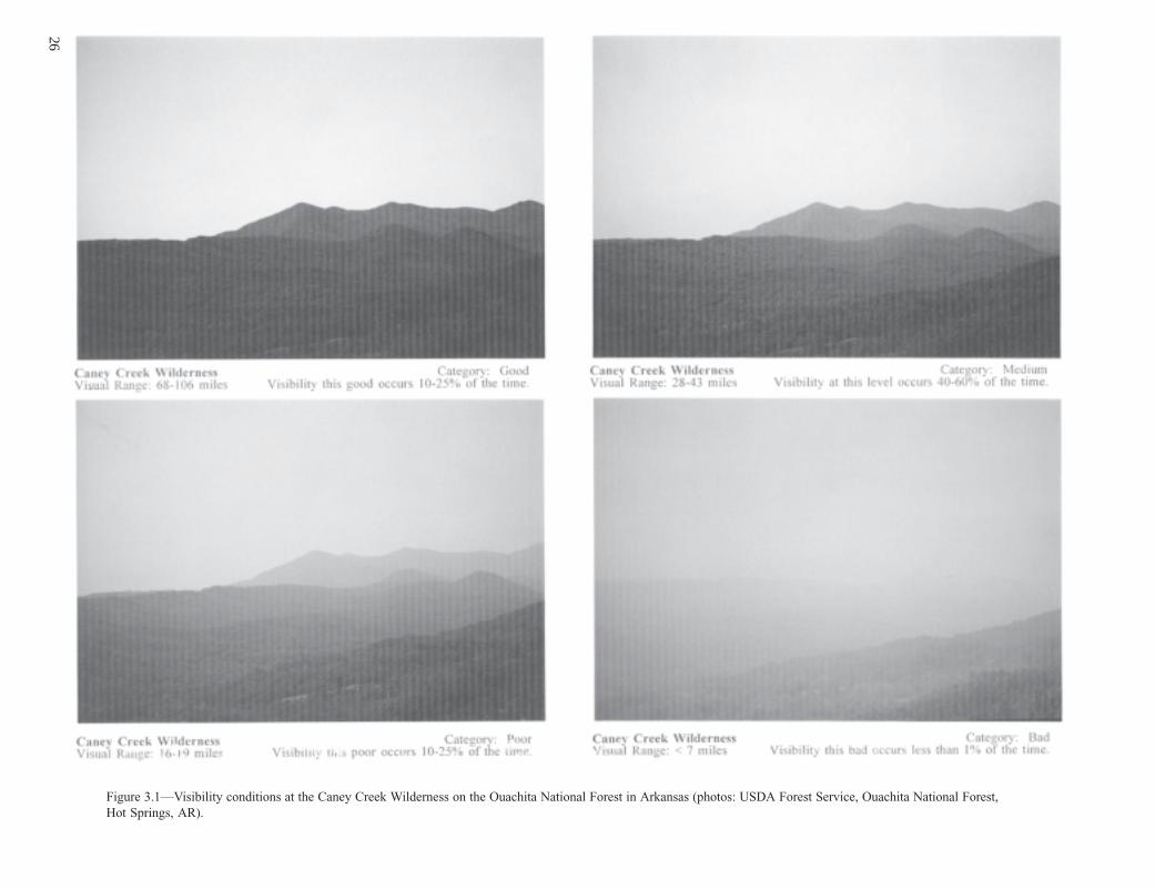
Figure 3.1—Visibility conditions at the Caney Creek Wilderness on the Ouachita National Forest in Arkansas (photos: USDA Forest Service, Ouachita National Forest,Hot Springs, AR).
26
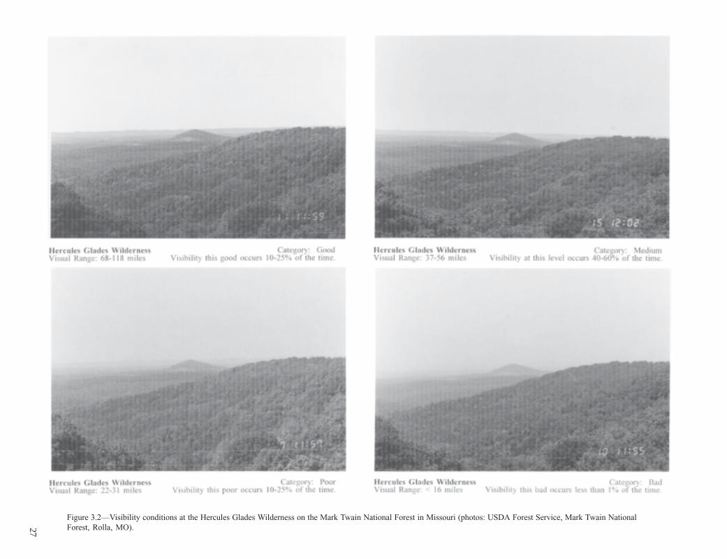
Figure 3.2—Visibility conditions at the Hercules Glades Wilderness on the Mark Twain National Forest in Missouri (photos: USDA Forest Service, Mark Twain NationalForest, Rolla, MO).27

Figure 3.3—Visibility conditions at the Upper Buffalo Wilderness on the Ozark-St. Francis National Forests in Arkansas (photos: USDA Forest Service, Ozark-St.Francis National Forests, Russellville, AR).
28

Figure 3.4—The fine particle (PM2.5) budget at the Upper Buffalo Wilderness IMPROVE site for winter (tophalf) and spring (lower half) from 1992 through 1995. The “fine mass budget” pie charts show the actualpercentages of particle components, based on weight. The “extinction budgets” show by what percentageeach constituent reduces the standard visual range (SVR).
Clear Day Extinction Budget
Hazy Day Fine Mass Budget Median Day Fine Mass Budget Clear Day Fine Mass Budget
Hazy Day Extinction Budget Median Day Extinction Budget
Soot5%
Soil4%
Nitrate27%
Sulfate34%
Organics30%
Organics26%
Soil2%
Soot5%
Nitrate27%
Sulfate40%
Coarse & soil
10%
Rayleigh29%
Nitrate18%
Sulfate18%
Organics12%Soot
13%
Sulfate25%
Nitrate21%
Soot15%
Rayleigh18%
Organics14%
Coarse & soil7%
Sulfate33%
Organics14%
Coarse & soil4%
Soot16%
Rayleigh10%
Nitrate23%
6.7 µg/m3 13.5 µg/m3
SVR = 113km SVR = 69km SVR = 38km
Sulfate28%
Soot7%
Soil6%
Organics31%
Nitrate28%
3.5 µg/m3
Hazy Day Fine Mass Budget
Hazy Day Extinction Budget
Clear Day Fine Mass Budget
Clear Day Extinction Budget Median Day Extinction Budget
Median Day Fine Mass Budget
Soot5%
Sulfate42%
Soil9%
Organics27%
Nitrate17%
Organics26%
Nitrate15%
Sulfate49%
Soot4%
Soil6%
Organics26%
Nitrate6%
Soil6%Soot
4%
Sulfate58%
Sulfate31%
Nitrate12%
Organics12%
Soot13%
Coarse & soil9%
Rayleigh23%
Sulfate40%
Nitrate12%
Soot14%
Coarse & soil6%
Rayleigh15%
Organics13%
Sulfate50%
Organics14%
Nitrate5%
Rayleigh9%
Soot16%
Coarse & soil6%
4.9 µg/m38.4 µg/m3 15.4 µg/m3
SVR = 88km SVR = 58km SVR = 34km
29

Figure 3.5—The fine particle (PM2.5) budget at the Upper Buffalo Wilderness IMPROVE site for summer(top half) and fall (lower half) from 1992 through 1995. The “fine mass budget” pie charts show the actualpercentages of particle components, based on weight. The “extinction budgets” show by what percentageeach constituent reduces the standard visual range (SVR).
Hazy Day Extinction Budget Median Day Extinction Budget Clear Day Extinction Budget
Clear Day Fine Mass Budget Median Day Fine Mass Budget Hazy Day Fine Mass Budget
Organics33%
Soil11%
Nitrate5%
Sulfate47%
Soot4%
Sulfate51%
Organics27%
Soot3%
Soil15%
Nitrate4%
Organics21%
Soot2%
Soil23%
Nitrate2%
Sulfate52%
Organics15%
Soot13%
Rayleigh19%
Coarse & soil7%
Nitrate5%
Sulfate41%
Organics14%
Nitrate4%
Sulfate51%
Coarse & soil7%
Soot14%
Rayleigh10%
Nitrate3%
Organics11%
Soot17%
Sulfate56%
Rayleigh5%Coarse &
soil8%
6.0 µg/m3 12.7 µg/m326.1 µg/m3
SVR = 73km SVR = 39km SVR = 21km
Hazy Day Extinction Budget
Hazy Day Fine Mass Budget Median Day Fine Mass Budget Clear Day Fine Mass Budget
Clear Day Extinction Budget Median Day Extinction Budget
Sulfate39%
Soil8%
Nitrate12%
Organics34%
Soot7%
Organics32%
Soot5%
Soil5%
Sulfate40%
Nitrate18%
Organics32%
Soot4%
Soil6%
Nitrate3%
Sulfate55%
Sulfate24%
Nitrate7%
Organics13%
Soot14%
Rayleigh32%
Coarse &soil
10%
Sulfate32%
Nitrate14%
Organics16%
Coarse & soil6%
Soot16%
Rayleigh16%
Nitrate3%
Organics18%
Soot17%
Sulfate48%
Coarse & soil5%
Rayleigh9%
3.2 µg/m3 7.7 µg/m316.0 µg/m3
SVR = 122km SVR = 63km SVR = 34km
30

As average PM2.5 concentrations increase from thewinter to spring months, visibility typically decreases. Thefine mass budgets shown in the lower half of figure 3.4indicate that average PM2.5 concentrations at the UpperBuffalo Wilderness site ranged from 4.9 µg m-3 to 15.4µg m-3 for “clear” and “hazy” days, respectively, from1992 through 1995. As in the winter months, increases insulfate concentrations were responsible for the reductionsin the SVR (88 km during “clear days,” 58 km during“median days,” and 34 km during “hazy days”). Sulfateaccounted for 42 percent of the PM2.5 mass budget on“clear days” and 58 percent of the PM2.5 mass budget on“hazy days.” Nitrate, on the other hand, decreased from17 percent of the PM2.5 mass budget on “clear days” to 6percent on “hazy days.”
The poorest visibility at the Upper Buffalo Wildernesssite typically occurs during the summer months, as shownin the top half of figure 3.5. The average SVR on “cleardays” from 1992 through 1995 was 73 km and decreasedto 21 km during “hazy days.” Changes in the PM2.5 massbudget associated with “clear” and “hazy” days includeda slight increase in the sulfate percentage (47 to 52percent), an increase in the soil percentage (11 to 23percent), and a decrease in the organics percentage (33to 21 percent). These constituent changes in the budgetresulted in average PM2.5 concentrations of 6.0 µg m-3 on“clear days” and 26.1 µg m-3 on “hazy days.” Althoughthe contribution of soil particles to the increase in PM2.5
concentrations on “hazy days” was significant, thepercentage contribution of soil particles to the SVRextinction budget did not change substantially from “cleardays” to “hazy days” at the site from 1992 through 1995(7 to 8 percent). In contrast to the soil particles, the slightincrease in the sulfate percentage of the fine mass budget(47 to 52 percent) from “clear” to “hazy” days resulted ina 41 to 56 percent change in the contribution that sulfatemade to the SVR extinction budget.
The lower half of figure 3.5 shows the fall fine massbudgets and extinction budgets for the Upper BuffaloWilderness site from 1992 through 1995. The averagePM2.5 concentration during fall “clear days” over thisperiod was similar to the average concentrations observedduring winter “clear days” (3.2 µg m-3 vs. 3.5 µg m-3), andaverage concentrations on fall “median days” (7.7 µg m-3)and “hazy days” (16 µg m-3) were similar to the observedspringtime concentrations (8.4 µg m-3 and 15.4 µg m-3,
respectively). The percentages of the all the fine massparticle components that make up the fall fine massbudget did not change significantly from “clear days” to“hazy days” over this period, except for the sulfate andnitrate percentages. The nitrate percentage decreasedfrom 12 percent of the total fine mass budget to 3 percenton “clear days” vs. “hazy days,” while the sulfate per-centage increased from 39 to 55 percent. This increase inthe contribution of sulfate to the total fine mass budgetfrom “clear days” to “hazy days” resulted in a 24 to 48percent change in the contribution of sulfate to thereduction in the average SVR (122 km on “clear days”and 34 km on “hazy days”).
Implications and Opportunities
To address the “remedying of any existing impair-ment” portion of the 1977 CAA amendments, the EPApublished a “Notice of Proposed [Regional Haze Regula-tions]” in the July 31, 1997, Federal Register, Vol. 62, No.147. These regulations proposed (1) that a “reasonableprogress target” be set to reduce visibility impairment dueto regional haze and (2) that visibility on the best 20percent of days not be degraded more than 0.1 dv. Inaddition, on the 20 percent of most impaired days,visibility must be improved at either the rate of 1 dv per10 years or 1 dv per 15 years (U.S. EPA 1997).
Title IV (Acid Deposition Control) of the CAAamendments of 1990 specifies that sulfur dioxide (SO2)emissions will be reduced by 10 million tons and nitrogenoxide (NOx) emissions by 2 million tons from 1980emission levels (U.S. EPA 1996). When these reductionsare fully implemented by the year 2000, visibility shouldbe improved. As figures 3.4 and 3.5 show, sulfates arethe major factor in visibility reduction, especially duringthe summer when visibility is poorest. Newly proposedPM2.5 and ozone regulations, while targeted to improvehuman health, should have the added benefit of improvingvisibility through anticipated reductions in atmosphericsulfate concentrations.
31


Chapter 4: Ground-Level Ozone
Question 4: What impact does ground-level ozonehave on forests?
Ozone, a naturally occurring chemical in the upperatmosphere and at ground level, is potentially the mostsignificant pollutant affecting forests in North America(Barnard and others 1991). Hourly average concentrationlevels of ozone near the ground are usually less than0.04 parts per million (ppm) in undeveloped areas of theworld with little anthropogenic pollution (Lefohn andothers 1990). Hourly average concentrations above0.05 ppm are frequently recorded at monitoring stationsin the Eastern United States (Lefohn and Jones 1986).
Ozone is formed by the reaction of nitrogen oxideswith volatile organic compounds on hot sunny days (NRC1991). Chameides and Cowling (1995) suggest thatground-level ozone formation is likely to be limited in theSouthern United States by the amount of nitrogen oxidesin the atmosphere. High amounts of nitrogen oxides areemitted in counties with large cities within and outside ofthe Ozark-Ouachita Highlands (fig. 1.6). The release ofnitrogen oxides, in combination with natural and anthropo-genic sources of volatile organic compounds, has thepotential to result in ozone concentrations that candamage or injure forest vegetation.
Ozone enters a leaf through openings called stomata.Several factors affect the uptake of ozone by a plant, butprimarily, a plant’s genetic makeup influences its re-sponse. Plant species vary in sensitivity to ozone; evenwithin a species, variations can occur. For instance,during field surveys, researchers have found one plantwith severe ozone symptoms growing adjacent to anindividual of the same species with no ozone symptoms.In an example outside the Assessment area, a portion ofthe most ozone-sensitive eastern white pines appears tohave been removed from the population due to ozoneexposures (U.S. EPA 1986). Other factors, such as light,temperature, relative humidity, soil nutrients, and soilmoisture also influence the uptake of ozone. The U.S.
Environmental Protection Agency (EPA) (1986) haspresented evidence that indicates that drought stress mayreduce the impact of ozone on plants (because the closedstomata prevent ozone entry into the leaves). Thevegetation could suffer growth losses, of course, due tothe lack of moisture.
Monitored concentrations in the atmosphere arerecorded as hourly average values in parts per million inthe data base. These concentrations represent “expo-sure,” defined as the amount of ozone that contacts theoutside of the leaf. As used here, the term “dose” is theamount of ozone that actually enters the leaf. Estimatesof dose are difficult to make without detailed modeling ofthe relationship between exposure and dose. Exposure isused as a surrogate for dose; researchers and policy-makers use exposures to assess the possible effects ofozone on vegetation.
Ozone inside the leaf is either destroyed by biochemi-cal processes or the ozone kills the cells found just belowthe upper leaf surface and between the veins of the leaf.Cells that are killed lose their green pigmentation andusually turn reddish or black in a process called stippling.The symptoms of ozone injury cannot be observed until alarge number of cells are dead. People who conduct fieldsurveys have a checklist of characteristics to identifyplants with ozone symptoms. The visible symptoms(stippling) indicate that the plant has had a physiologicalresponse to the ozone dose, resulting in injury. Damageresults when the ozone dose was large enough to reducethe intended human use or the value of the plant orecosystem (Tingey and others 1991).
Several surveys of ozone symptoms have beenconducted within and near the Ozark-Ouachita High-lands. Between 1991 and 1995, the incidence of ozonesymptoms at the Caney Creek Wilderness and UpperBuffalo Wilderness was low. The percentage of black-berry plants with ozone symptoms was highest in 1991,with 14 percent showing symptoms at Caney Creek and24 percent at Upper Buffalo. In 1995, there were noozone symptoms on any of the blackberry plants (Kertzand others 1995).
33
This chapter will focus on the possible extent andfrequency of damage from ozone to trees in forestsettings. The Atmospheric Team uses the term “damage”to mean that ozone exposure has likely been sufficient tocause reduced tree growth (Dowsett and others 1992).
Key Findings
1. Using available ozone monitoring data, it appearsthat ground-level ozone had a minimal impact onforest tree growth between 1990 and 1995.
2. There are few ozone monitors within the Assess-ment area. Consequently, there could be localizedareas where growth losses occurred to trees that arehighly sensitive to ozone.
3. Future ozone exposure may be less as Federal,State, and local air pollution control agencies imple-ment strategies to reduce pollution, especiallynitrogen oxide (which will, in turn, reduce theformation of ground-level ozone).
Data Sources and Methods of Analysis
Ozone formation is strongly influenced by meteorologi-cal conditions and the amounts of ozone precursorspresent in the atmosphere (NRC 1991). For example,1988 was a hot and dry year during which large sectionsof the Eastern United States had high ozone exposures.In comparison, 1989 was cool and moist, and the ozoneexposures were low (Lefohn and others 1997). Therange in yearly ozone exposures required that more than1 year be examined to describe the current condition forthe study area. Therefore the team selected 1990 through1995 as the period for analysis.
For this Assessment, data in the EPA’s AerometricInformation Retrieval System (AIRS) data base and fromthe National Dry Deposition Network program wereused. The monitoring sites included those in the States ofArkansas, Illinois, Kansas, Kentucky, Louisiana, Missis-sippi, Missouri, Oklahoma, Tennessee, and Texas. Themonitoring sites selected from these States had 75percent or greater data capture for each particular year.Numerous statistics were calculated using the 24-hourperiod over the growing season, defined as the months of
April through October. Initially, many researchers usedlong-term average concentrations to describe ozoneexposures when assessing vegetation effects (Heck andothers 1982). The EPA (1989) examined the peer-reviewed literature and concluded that long-term aver-ages are not adequate indicators for relating ozoneexposure to plant response. Furthermore, the EPA (1986and 1992) concluded that greater effects to vegetationoccur when the exposures include short-term, highconcentrations rather than long-term, low concentrations.The team chose to use the mathematical index W126, asdescribed by Lefohn and Runeckles (1987), to evaluatewhether trees within the Assessment area may besuffering from growth losses (damage). All of theavailable hourly ozone estimates were used to calculatethe seasonal W126. Results obtained from the W126calculations (or any other cumulative exposure index) canhave high values, but concentrations equal to or above0.10 ppm may not occur. Consequently, the AtmosphericTeam followed the recommendation of Lefohn and Foley(1992) and included the number of hours greater than orequal to 0.10 ppm in the analysis.
Numerous studies have been conducted to examinethe relationship between ozone exposures and treeresponse. Lefohn and others (1997) reviewed thecontrolled exposure studies and recommended a tech-nique that divided the landscape into four categories,based on the W126 statistic and the number of hours theozone concentration was greater than or equal to 0.10ppm. To accomplish this task, it was necessary toextrapolate the ozone monitoring data beyond the moni-toring sites. Extrapolations of the W126 values across theAssessment area were accomplished using a statisticaltechnique described in a report by Lefohn and others(1995). The W126 estimates were made for the center ofgrid cells of 0.5 degrees latitude by 0.5 degrees longitudeacross much of the region (fig. 4.1). Estimates were notavailable for the northern portion of the Assessmentarea. The add-on software to ArcView® called SpatialAnalyst® was used to interpolate the W126 valuesbetween the points and for the northern portion of theAssessment area. A spline technique was used for theinterpolations to a 6.2-mile (mi) by 6.2-mi grid. Twelvepoints were used for the spline interpolation, but esti-mates only were made for the area within the Assess-ment boundary.
34

The team then categorized the interpolated W126values (grids) as follows:• Minimal—Ozone exposure is so low that little or no
growth loss is predicted to occur in any species.Ozone symptoms may have been present even thoughthe exposures were low.
• Level 1—Ozone exposure is high enough to causegrowth reductions in species considered highly sensi-tive to ozone, such as black cherry.
• Level 2—Ozone exposure is high enough to causegrowth reductions in species with moderate sensitivityto ozone, such as tulip poplar, in addition to thosespecies that are included in Level 1.
• Level 3—Ozone exposure at this level is high enoughto cause growth loss in many species—even thosenormally considered resistant to ozone exposures suchas red oak—in addition to those species in Level 1 andLevel 2.
Figure 4.1—Locations of W126 estimates.
The Atmospheric Team used a subjective analysis toclassify the amount of area within a tree responsecategory (table 4.1). The criteria listed in table 4.1required consistency with both the W126 and the numberof hours with concentrations greater than or equal to 0.10ppm. Because the number of hours greater than or equalto 0.10 ppm was not statistically extrapolated across thestudy area, it was necessary to finish the classification byvisually examining the monitored values for the number ofhours greater than or equal to 0.10 ppm. Grids that hadone or more ozone monitors present were classified usingthe results from the ozone monitors, but cells that did nothave an ozone monitor were classified by examining thepattern from ozone monitors surrounding the cell to beclassified. Grids that met the W126 criteria for a particu-lar category and not the number of hours greater than orequal to 0.10 ppm for the same category were assignedthe category that matched the number of occurrencesgreater than or equal to 0.10 ppm.
The experimental studies summarized by Lefohn andothers (1997) used plants grown under optimum condi-tions of adequate soil moisture and nutrients. Before theteam applied the criteria in table 4.1, they gathered
Table 4.1—Forest tree response categories based on W126values and exposure hours required for various levels of foresttree damage
W126 ExposureForest tree response category values hours
ppm >0.10 hours ppm
Minimal > 0 and > 0Level 1 (only highly sensitive
species affected, e.g., blackcherry) > 5.9 and > 6
Level 2 (moderately sensitivespecies affected, e.g., yellow-
poplar) > 23.8 and > 51Level 3 (resistant species
affected, e.g., red oak) > 66.6 and 135
W126 = ozone exposure index; ppm = parts per million; exposure hours= number of hours the hourly average ozone concentrations is > 0.10ppm.Source: Lefohn and others (1997).
35

Figure 4.2—Palmer Hydrologic Index results for April through July1990.
information on whether the environmental conditionswere favorable for ozone to enter the leaf. Of theenvironmental conditions that need to be considered, soilmoisture has been identified as an important variable thatinfluences the uptake of ozone by a plant (U.S. EPA1986). Showman (1991) and Jackson and others (1992)have observed fewer ozone symptoms on sensitivespecies during periods of drought than in seasons withadequate rainfall, even though ozone exposures werehigher during the drought. Thus, the Atmospheric Teamchose the Palmer Hydrologic Index (Palmer 1965) as asurrogate measurement of soil moisture. The index is amonthly value computed for specific climate divisions(regions within a State with similar climatic and hydro-logic characteristics). Also, the index indicates theseverity of a wet or dry spell. A Palmer HydrologicIndex of less than -2 (minus two) was considered toindicate low soil-moisture conditions, that is, a drought(Briffa and others 1994). The team hypothesized thatozone exposure would not damage the plants during adrought. Values above -2 indicated adequate soil mois-ture, when ozone could potentially penetrate leaves anddamage plants. The average Palmer Hydrologic Indexfor April through July was calculated for each climatedivision.
Combining the results from the Palmer HydrologicIndex (fig. 4.2) and ozone exposure (fig. 4.3) provides anindication that (1) soil moisture was sufficient for plantsto keep their stomata open enough for ozone to penetratethe leaves and (2) ozone exposures were severe enoughto cause growth losses. Areas classified as experiencinga drought (dry) were assigned the growth responsecategory of “minimal” effect from ozone; otherwise thesensitivity category value remained the same afterapplying the criteria in table 4.1.
Patterns and Trends
The average April to July Palmer Hydrologic Indexvalues from 1990 to 1995 indicate that normal to wetconditions were prevalent over the Assessment area (fig.4.2 shows the average April to July Palmer HydrologicIndex values for 1990 only). Consequently, the teamhypothesized that the stomata were open at times duringthe growing season, and ozone could have penetrated intothe leaves. The results from statistical estimates placed
almost all of the Assessment area into W126 values of5.9 to 23.8 ppm hours (Level 1) for the years 1991through 1993 (figs. 4.4, 4.5, and 4.6). Whereas, in 1990,1994, and 1995 (figs. 4.3, 4.7, and 4.8), most of theAssessment area had W126 values between 23.8 and66.5 ppm hours (Level 2), no areas were classified ashaving less than 5.9 ppm hours (minimal). Using only theW126 values would indicate that Level 1 and/or Level 2tree species may have had growth losses for the 6 years.However, hourly average ozone concentrations wereseldom greater than or equal to 0.10 between 1990 and1995.
Most of the ozone monitors within and near theAssessment area indicated less than 6 hours during thegrowing season when the average hourly concentrationswere greater than or equal to 0.10 ppm (figs. 4.3 to 4.8).Therefore, by following the recommendation of Lefohnand Foley (1992) and the procedure of Lefohn and others(1997), the team decided it is likely that ground-levelozone exposures had a minimal impact to forest trees andthat no growth losses resulted from ozone exposures. Thelack of ozone symptoms reported by Kertz and others
36

Figure 4.3—Ozone estimates for 1990 showing sites classified according to tree response categories (see table 4.1)and W126 values.
(1995) provides additional evidence that ozone likely hada minimal impact on forest tree growth.
The team believes caution should be used in interpret-ing these findings since there were less than 10 ozonemonitors collecting data within the Assessment areabetween 1990 and 1995. There could be localized areaswithin the Ozark-Ouachita Highlands with more than 5hours of hourly averaged ozone concentrations greaterthan or equal to 0.10 ppm. If such events did occur, thepotential for growth losses to the most sensitive species
(Level 1) may have been realized in localized areas,possibly near St. Louis, MO, and Tulsa, OK. Conversely,it is important to note that the W126 exposure indexvalues for this study were accumulated for the growingseason—April through October. Most of the experimentaldata used in this Assessment were collected for 3 to 4months (Lefohn and others 1997). Thus, using a 7-monthperiod to accumulate the W126 value may overestimatethe likelihood of predicted growth losses.
37

Figure 4.4—Ozone estimates for 1991 showing sites classified according to tree response categories (see table 4.1) andW126 values.
Implications and Opportunities
Current emission strategies implemented by local,State, and Federal air pollution agencies may reduceozone exposures in rural forests in the future. For ex-ample, there could be a lowering of ozone exposures inthe Ozark-Ouachita Highlands as ozone nonattainmentareas outside the study area (such as Dallas) implementcontrol strategies that bring the urban area back intocompliance with Federal law. Furthermore, the revision ofthe National Ambient Air Quality Secondary (NAAQS)
standard to an 8-hour average of .085 ppm is likely tobenefit forests. To lessen the risk of tree growth loss, airpollution control agencies will have to implement emissionreduction strategies in areas that violate the new primarystandard and decrease the number of hours of averageozone concentrations greater than or equal to 0.10 ppm.
Ozone exposures in the study area result from thechemical reaction of nitrogen oxides and volatile organiccompounds. The volatile organic compounds are knownto be so abundant (figs. 1.8 and 1.10) that it appearsnitrogen oxides may be the limiting factor in ozone
38

Figure 4.5—Ozone estimates for 1992 showing sites classified according to tree response categories (see table 4.1) andW126 values.
formation (Chameides and Cowling 1995). Implementa-tion of and compliance with the Clean Air Act Amend-ments of 1990 should reduce nitrogen oxide emissionsnationally by 2 million tons and may reduce ozone expo-sures further within the Assessment area. Other strate-gies that reduce nitrogen oxides may also result in lowerozone exposures for the Ozark-Ouachita Highlands area.Recently, the EPA notified State and local air pollutioncontrol agencies in 22 Eastern States that further reduc-
tions in nitrogen oxides are needed for some urban areasto satisfy the NAAQS for ground-level ozone. Of theStates included in this analysis, the EPA requested thatIllinois, Kentucky, Missouri, and Tennessee reducebetween 35 and 43 percent of emissions of nitrogenoxides. Implementation of nitrogen oxide reductions ofthis magnitude likely will reduce the amount of ground-level ozone in the Assessment area.
39

Figure 4.6—Ozone estimates for 1993 showing sites classified according to tree response categories (see table 4.1)and W126 values.
40
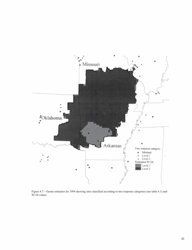
Figure 4.7—Ozone estimates for 1994 showing sites classified according to tree response categories (see table 4.1) andW126 values.
41

Figure 4.8—Ozone estimates for 1995 showing sites classified according to tree response categories (see table 4.1) andW126 values.
42

Chapter 5: Acid Deposition
Question 5: To what extent are resources in theHighlands being affected by acid deposition?
Sulfur dioxide (SO2) and nitrogen oxides (NOx)present in the atmosphere can react with water, oxygen,and oxidants (such as ozone) to form mild solutions ofsulfuric acid and nitric acid (U.S. EPA 1998a). Theseacidic solutions are often found in rainwater, snow, fog,and other forms of precipitation. When precipitationcontaining these acidic compounds falls to the earth, theacidic compounds are deposited on the earth’s surface(acid deposition or wet deposition), and the precipitationcarrying the acidic compounds is referred to as “acidrain.” Scientists have discovered that air pollution fromthe burning of fossil fuels is the major cause of acid rain.Acidic compounds in the atmosphere and the depositionof acidic compounds on the earth’s surface can disruptforest and aquatic ecosystem functions, impair visibility,and create human health problems.
Chapter 1 provides a regional perspective on sourcesand amounts of nitrogen (fig. 1.6) and sulfur compounds(fig. 1.12) emitted into the atmosphere. It is worthrestating that 28 percent of nitrogen oxide (NOx) emis-sions in the Assessment area and nearby are fromindustrial fuel combustion sources, 22 percent are fromvehicles (internal combustion engines), and 20 percentare from electric utilities (fig. 1.5). As figure 1.11 shows,sulfur dioxide (SO2) is primarily produced from electricpower generation (72 percent), with all other industrysources producing 15 percent (U.S. EPA 1996).
Since the mid- to late 1970’s, emissions of SO2 andNOx have decreased and leveled off, respectively, incontrast to the upward trends in emissions of these gasesexperienced from the early 1950’s to the mid-1970’s (fig.1.17). Vehicle miles traveled have doubled since 1970, but
exhaust emissions have only slightly increased (U.S. EPA1996) because of better fuel economy and more efficientengines. Since 1996, this same strategy has been appliedto selected nonroad categories (e.g., small engines suchas lawn mowers and outboard motors). The Environmen-tal Protection Agency (EPA) (1996) expects significantemission reductions after the year 2000. Sulfur emissionshave also been reduced per unit of production. From 1970to 1995, SO2 emissions from electric utilities decreasedabout 31 percent (U.S. EPA 1996). Implementation ofthe Clean Air Act amendments of 1990 should reduceSO2 emissions by 10 million tons and NOx by 2 milliontons by the year 2000 (U.S. EPA 1996).
The impact of acid deposition on forest and aquaticecosystems has been the subject of much research anddebate. The 1980 to 1990 National Acid PrecipitationAssessment Program (NAPAP) provided indepthresearch on these impacts (see Baker and others1991). As NAPAP and others have reported, thepotential harmful effects of acidic deposition include:(1) leaching of nutrients from plant foliage and the soil byhydrogen, sulfate, or nitrate ions (Lee and Webber 1982);(2) alteration of beneficial micro-organisms in the forestfloor and upper soil horizons, including damage to symbi-otic nitrogen-fixing organisms (Francis 1982); (3) acid-induced mobility and toxicity of aluminum in the soilsolution leading to toxic levels of aluminum in streamflowand water bodies (Steiner and others 1980; Ulrich andothers 1980; Johnson and others 1981); (4) increasedsusceptibility of trees and plants to environmentalstresses, including drought (Johnson and others 1981; Leeand Webber 1982); (5) delayed frost hardiness leading tovegetation damage (DeHayes 1992); and (6) acidificationof aquatic ecosystems (Herlihy and others 1996). Im-pacts may thus affect entire ecosystems includingvegetation, soil, and the receiving watercourse.
43

Key Findings
1. Atmospheric wet acid loadings are less than theloadings observed in the Southern Appalachianregion. Nitrate and sulfate loadings are expected todecrease in the future based on expected decreasesin emissions of sulfur dioxide and nitrogen oxides(see Chapter 1).
2. Most surface waters within the Assessment area donot appear to be adversely impacted by the previousand present rate of acid deposition.
3. The low acid neutralizing capacity headwater areasof the Ouachita Mountains make them most at riskwhile the limestone areas of the Ozark Plateau areleast at risk.
Data Sources and Methods of Analysis
Because nitrate and sulfate depositions over a regionare related to precipitation patterns, it was necessary toassess the spatial variations in precipitation over theAssessment area at a sufficient resolution to account formajor elevation changes. The deposition model of Lynchand others (1997), used in this Assessment for generatingnitrate and sulfate deposition maps, incorporates precipita-tion patterns that account for the changes in topographicvariations observed in the Assessment area. The coordi-nates, elevations, and monthly precipitation records fromthe National Oceanic and Atmospheric Administration’s(NOAA) precipitation monitoring sites in the States withinand adjacent to the Assessment area constitute theprecipitation-volume data set used to develop the deposi-tion model. Lynch and others (1997) obtained precipitationconcentration data for sulfates and nitrates from weeklyrainfall samples collected at monitoring sites within andadjacent to the Assessment area.
The deposition model uses a statistical method thatincludes: (1) the precipitation observed at monitoring sites,(2) elevation, and (3) a set of variables representing bothslope and aspect. The derived regression equations fromeach 0.1-degree block are then applied to correspondingdigital elevation data to produce a grid of precipitationestimates. The current model compares the predicted andobserved quarterly and annual precipitation volumes atapproximately 1,500 validation sites scattered over the
Assessment area. The average annual estimation error isconsistently near 3.0 inches (in.) for each year from 1991through 1993 (Lynch and others 1997).
The NOAA data set comprises the only precipitationvalues that cover the Assessment area at a site densitysufficient for deposition modeling. A major limitation onthe accuracy of the model’s precipitation calculations isthe imprecise coordinates of the NOAA precipitationsites. NOAA coordinates for the location of a rain gaugeare reported at a resolution no finer than 1 minute of adegree of latitude or longitude. This level of uncertaintyimpedes the modeling of localized—but important—geographic influences on precipitation. The modificationsthat Lynch and others (1997) made to the model over-came the imprecision of the coordinates and estimatedmore precise coordinates of each NOAA precipitationmonitoring station.
Because precipitation varies year to year, the amountof deposition also varies. Deposition rates, therefore, aremodeled values, not measured values; they should beconsidered relative rather than absolute values and usedwith caution. Actual values determined at the site ofconcern will be needed to document any influence on thelocal ecosystem.
Patterns and Trends
Figures 5.1 and 5.2 indicate that the southwestern partof the Assessment area has the highest sulfate andnitrate deposition. Figure 5.2 shows that sulfate depositionexceeds 20 pounds per acre (lbs/ac) in the high elevationand high precipitation areas of the southwest portion ofthe Ouachita range. An EPA finding suggests this patterncould be a result of sulfur dioxide emissions from coal-burning industries in Louisiana and Texas (OK WRB1990). The other area receiving high sulfates but not highnitrate deposition is the northeastern portion of theAssessment area, including the Potosi-FredericktownDistrict and the eastern half of the Salem District of theMark Twain National Forest.
Figure 5.3 shows the average modeled sulfate andnitrate deposition within the Assessment area from 1983to 1995. Compared to the Southern Appalachians, theannual sulfate deposition in the Ozark-Ouachita High-lands is moderate—15 lbs/ac in the Highlands comparedto 20 to 25 lbs/ac for the Southern Appalachians. The
44

average annual nitrate deposition in the Assessment areais 10 lbs/ac compared to 15 to 20 lbs/ac in the SouthernAppalachians (SAMAB 1996).
During the NAPAP era (1980 to 1990), there was aneffort to look for evidence that acidic deposition wasaffecting surface waters within the Assessment area.Between 1984 and 1986, the EPA conducted one of thelargest limnological reconnaissance projects ever under-taken—the National Surface Water Survey (NSWS)—the results of which are available from the EPA. TheNAPAP and NSWS used the acid neutralizing capacity(ANC) to rate streams and lakes. This survey found thata relatively high percentage of streams with ANC equalto or greater than 200 existed in the interior Southeastregion, which includes the Assessment area, while nolakes or streams in this region had ANC values less than
or equal to zero (Baker and others 1991). However, thissame report indicated that the Ozark-Ouachita area had19 percent of the streams with ANC greater than zeroand less than or equal to 50 (Baker and others 1991).These poorly buffered systems can be considered at riskfor acidification.
Within the Assessment area, the headwater sectionsof the Ouachita Mountains in Arkansas contain very littlelimestone bedrock, while the Ozark Plateau area inMissouri contains large areas of limestone and karsttopography (irregular limestone with sinks, undergroundstreams, and caverns). These geological differencessuggest that the Ouachita Mountain headwaters are likelyto be more at risk for acidification than streams in theOzark Plateau.
Figure 5.1—The period average for nitrate deposition (lbs/ac) in the Assessment area from 1983 through1995 (Lynch and others 1997).
45
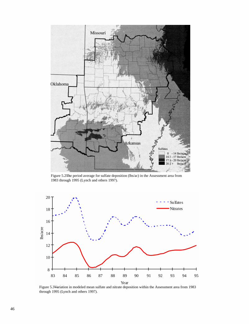
8
10
12
14
16
18
20
83 84 85 86 87 88 89 90 91 92 93 94 95
Year
lbs/
acre
Sulfates
Nitrates
46
Figure 5.2—The period average for sulfate deposition (lbs/ac) in the Assessment area from1983 through 1995 (Lynch and others 1997).
Figure 5.3—Variation in modeled mean sulfate and nitrate deposition within the Assessment area from 1983through 1995 (Lynch and others 1997).

Another test of acidification is the amount of nitratesand sulfates moving through a system. The consensus ofNAPAP is that the streams in the Ozark-OuachitaHighlands are at equilibrium for sulfates and that 99percent of the nitrates are being retained. Sulfate enrich-ment is occurring in some waters in the Ozark-OuachitaHighlands (Baker and others 1991).
Nix and Thornton (1987) confirmed the overallNAPAP and NSWS assessment that the higher elevationstreams in the Ouachitas are vulnerable to acid deposi-tion. Their major findings were that: (1) during stormevents, ionic aluminum is released into surface waters;(2) 90 percent of nitrogen is being retained; (3) sulfatesare near equilibrium; and (4) base cations are beingexported at twice the rate of precipitation input. Theyconcluded that headwater streams that have low ANCare potentially at risk with respect to acidic deposition.
Precipitation patterns strongly influence acid deposi-tion. As explained in the “Data Sources and Methods”section of this chapter, elevation changes can impactprecipitation amounts. The Ouachita Mountains in thesouthwestern part of the Assessment area can produceorographic lifting (the lifting of air when it flows overhigher elevation terrain) of moist air moving northwardfrom the Gulf of Mexico across the Gulf Coastal Plain.The Atmospheric Team expects this area will receive thegreatest amount of deposition. Kress and others (1988)found that an average 400-foot increase in elevation fromthe Gulf Coastal Plain to the Ouachita Mountains insoutheastern Oklahoma resulted in a 12-percent increasein average annual precipitation (60.2 to 67.6 in. in 1984 to1985). They also found the average pH decreased withincreased elevation of the station (4.67 at the CoastalPlain to 4.53 at the Ouachita Mountains). Total nitratedeposition increased from 3.2 to 3.5 lbs/ac, and totalsulfate deposition increased from 28.3 to 32.7 lbs/ac aselevation increased.
Implications and Opportunities
Acid deposition can pose a threat to forest and aquaticecosystems—especially on poorly buffered, higherelevation watersheds. Acid deposition patterns in theAssessment area as a result of sulfate and nitrate in theatmosphere are affected by the emissions of SO2 andNOx and the patterns of precipitation over the region. Asnoted in Chapter 1, emissions of SO2 from electricalutilities in the Assessment area are expected to decreaseas the Clean Air Act Amendments of 1990 are fullyimplemented. Furthermore, the emissions of nitrogenoxides from fuel combustion at industrial sources in theAssessment area will likely be reduced in response tocurrent efforts by the EPA. Future reductions in theemissions of sulfur dioxide and nitrogen oxides shouldlead to reduced atmospheric sulfate and nitrate concen-trations, thereby reducing the potential for acid depositionepisodes. However, future changes in precipitationpatterns as a result of changes in regional climate andclimate variability may also impact the amount of aciddeposition over the Assessment area.
A comprehensive assessment of how acid depositionpatterns might change over the Assessment area as aresult of changing emissions of SO2 and NOx and achanging climate (including precipitation patterns) willrequire the use of coupled, high-resolution atmosphericmesoscale and chemistry models that can generateplausible scenarios of acid deposition, e.g., the U.S. EPA(1998b) Regional Acid Deposition Model. The develop-ment of these future scenarios of acid deposition musttake into account the complex atmospheric dynamicsassociated with the emission, transport, and diffusion ofthe chemical species involved in the formation of acidrain; the dynamics of cloud formation and precipitationoccurrence over the region; surface-atmosphere interac-tions that influence the hydrologic cycle in the region; andthe overriding chemical reactions that lead to the forma-tion of sulfuric and nitric acid in the atmosphere. The aciddeposition scenarios generated by coupled atmosphericmesoscale and chemistry models can provide vitalinformation to natural resource managers as they developmanagement strategies for specific watersheds in theAssessment area known to be sensitive to potential aciddeposition events.
47


References
Baker, Lawrence A.; Kaufmann, Philip R.; Herlihy, Alan T. [andothers]. 1991. Current status of surface water acid-basechemistry. In: Irving, Patricia M., ed.-in-chief. Aquaticprocesses and effects. Volume II of Acidic deposition: stateof science and technology. Washington, DC: U.S. NationalAcid Precipitation Assessment Program: Rep. 9: 9-5 – 9-D-2.
Barnard, Joseph E.; Lucier, Allen A.; Brooks, Robert T. [andothers]. 1991. Changes in forest health and productivity inthe United States and Canada. In: Irving, Patricia M., ed.-in-chief. Terrestrial materials, health and visibility effects.Volume III of Acidic deposition: state of science andtechnology. Washington, DC: U.S. National AcidPrecipitation Assessment Program: Rep. 16: 16-3 – 16-186.
Braun, Stephen. 1996. Winds of change imperil Ozark charcoalovens. Arkansas Democrat-Gazette. December 28: 5B.
Briffa, K.R.; Jones, P.D.; Hulme, M. 1994. Summer moistureavailability across Europe, 1892–1991: an analysis based onthe Palmer Drought Severity Index. International Journal ofClimatology. 14: 475–506.
Burrough, P.A. 1988. Principles of geographical informationsystems for land resource assessment. New York: OxfordUniversity Press. 194 p.
Chameides, W.L.; Cowling, Ellis B. 1995. The state of theSouthern Oxidant Study (SOS): Policy-relevant findings inozone pollution research 1988–1994. Southern OxidantStudy. Raleigh, NC: College of Forest Resources, NorthCarolina State University. 136 p.
Cooperative Institute for Research in the Atmosphere (CIRA).[Accessed October 1997]. PM10.CGM; PM2.5.CGM. <ftp://alta_vista.cira.colostate.edu/data/improve/usmaps/annual>.Ft. Collins, CO: Colorado State University. 2 p.
DeHayes, Donald H. 1992. Winter injury and developmentalcold tolerance of red spruce. In: Eager, Christopher; Adams,Mary Beth, eds. Ecology and decline of red spruce inEastern United States. New York: Springer-Verlag:295–337.
Dowsett, Sally E.; Anderson, Robert L.; Hoffard, William H.1992. Review of selected articles on ozone sensitivity andassociated symptoms for plants commonly found in theforest environment. R8-TP 18. Atlanta, GA: U.S. Departmentof Agriculture, Southern Region, Forest Pest Management.22 p.
Fisher, Rich. USDA Forest Service personal communication,September 30, 1997. [Manuscript on file at the Zone AirSpecialist’s office on the Ouachita National Forest, HotSprings, AR.]
Florida Department of Environmental Protection (FL DEP). 1993.Apalachicola National Forest controlled burn study usingPM10 saturation samples. Tallahassee, FL: FloridaDepartment of Environmental Protection, Air MonitoringSection. 10 p. [Unpublished report on file at the Zone AirSpecialist’s office on the Ouachita National Forest, HotSprings, AR.]
Francis, A.J. 1982. Effects of acidic precipitation and acidity onsoil microbial processes. Water, Air, Soil Pollution. 18: 374–394.
Haddow, Dennis. April 2–11, 1990. Unit II–J, air resourcemanagement, fire in resource management. Marana, AZ:National Advanced Resource Technology Center. 9 p.[Manuscript from this course on file at the Zone AirSpecialist’s office on the Ouachita National Forest, HotSprings, AR.]
Heck, W.W.; Taylor, O.C.; Adams, R.M. [and others]. 1982.Assessment of crop loss from ozone. Journal of the AirPollution Control Association. 32: 353–361.
Herlihy, Alan T.; Kaufmann, Philip R.; Stoddard, John L. [andothers]. 1996. Effects of acidic deposition on aquaticresources in the Southern Appalachians with a special focuson Class I wilderness areas. Asheville, NC: The SouthernAppalachian Initiative. 91 p.
Holzworth, G.C.; Fisher, R.W. 1979. Climatological summaries ofthe lower few kilometers of Rawinsonde observations. EPA600/4-79-026. Washington, DC: U.S. EnvironmentalProtection Agency.
Hunt, Clifford F.; Barber, Brad; Ford, Larry. 1994. Monitoringsmoke from prescribed fires on National Forests in Texas,spring 1994. Lufkin, TX: U.S. Department of Agriculture,Forest Service, National Forests in Texas. [Manuscript onfile at the Zone Air Specialist’s office on the OuachitaNational Forest, Hot Springs, AR.] 9 p.
Jackson, W.A; Iskra, A.; Edwards, P.J. 1992. Characterization ofozone symptoms on native vegetation at the Dolly Sods andOtter Creek wildernesses. In: Berglund, R., ed. Troposphericozone and the environment II. Pittsburgh, PA: Air and WasteManagement Association: 526–536.
49

Johnson, Noye M.; Driscoll, Charles T.; Eaton, John S. [andothers]. 1981. “Acid rain,” dissolved aluminum and chemicalweathering at the Hubbard Brook Experimental Forest, NewHampshire. Geochemica et Cosmochimica. Acta. 45: 1421–1437.
Kertz, Ronald C.; Starkey, Dale A.; Bruce, William A. [andothers]. 1995. Ozone damage to vegetation associated with 4Forest Service wilderness areas in Alabama, Arkansas andTexas. Forest Pest Management Report No. 96-2-01.Alexandria, LA: U.S. Department of Agriculture, ForestService, Alexandria Field Office. 15 p.
Kress, M.W.; Wigington, P.R., Jr.; Miller, E.L. 1988.Atmospheric deposition in the Ouachita Mountains ofsoutheast Oklahoma. Proceedings of the OklahomaAcademy of Science. 68: 63–68.
Lee, J.J.; Webber, D.E. 1982. Effects of sulfuric acid rain onmajor cation and sulfate concentrations of water percolatingthrough two model hardwood forests. Journal ofEnvironmental Quality. 11: 57–64.
Lefohn, A.S.; Foley, J.K. 1992. NCLAN results and theirapplication to the standard-setting process: protectingvegetation from surface ozone exposures. Journal of AirWaste Management Association. 42(8): 1046–1052.
Lefohn, A.S.; Jackson, William; Shadwick, Douglas S. [andothers]. 1997. Effect of surface ozone exposures onvegetation grown in the Southern Appalachian mountains:identification of possible areas of concern. AtmosphericEnvironment. 31(11): 1695–1708.
Lefohn, A.S.; Jones, C.K. 1986. The characterization of ozoneand sulfur dioxide air quality data for assessing possiblevegetation effects. Journal of the Air Pollution ControlAssociation. 36: 1123–1129.
Lefohn, A.S.; Knudsen, H.P.; Shadwick, D.S. 1995. Usingkriging to estimate the 7-month (April-October) SUM06 andW126 indices for the Southeastern United States from 1983until 1993. Prepared for the Tennessee Valley Authority. 76p. [Report on file with the Zone Air Resource Specialist,National Forests in North Carolina, Asheville, NC.]
Lefohn, A.S.; Krupa, S.V.; Winstanley, D. 1990. Surface ozoneexposures measured at clear locations around the world.Environmental Pollution. 63: 189–224.
Lefohn, A.S.; Runeckles, V.C. 1987. Establishing a standard toprotect vegetation-ozone exposure/dose consideration.Atmospheric Environment. 21: 561–568.
Lynch, James A.; Grimm, Jeffrey W.; Corbett, Edward S. 1997.Enhancement of regional wet deposition estimate based onmodeled precipitation inputs. University Park, PA: ThePennsylvania State University, School of Forest Resources.[Manuscript on file with the Zone Air Specialist, OuachitaNational Forest, Hot Springs, AR.]
Miller, Michael V. 1997. U.S. Forest Service, Region 8 PollutionExposure Index Model, Version III Workplan. 21 p. [Reporton file with the Zone Air Resource Specialist, NationalForests in North Carolina, Asheville, NC.]
Muncy, Jack A. 1986. A plan for revegetation completion ofTennessee’s Copper Basin. Norris, TN: Tennessee ValleyAuthority, Division of Land and Economic Resources.32 p.
National Research Council (NRC). 1991. Rethinking the ozoneproblem in urban and regional air pollution. Washington,DC: National Academy Press. 500 p.
Nix, Joe F.; Thornton, Kent W. 1987. Storm event sampling oftwo low alkalinity southwestern Arkansas streams. EPACooperative Agreement 811863-01-0. Little Rock, AR: FTNAssociates, Ltd. 143 p.
Oklahoma Water Resources Board (OK WRB). 1990. OklahomaWater Atlas Publication 135. Norman, OK: Oklahoma WaterResources Board. 360 p.
Palmer, Wayne C. 1965. Meteorological drought. U.S. WeatherBureau Report No. 45. Washington, DC: U.S. Department ofCommerce. 58 p.
Pitchford, Marc L.; Malm, William C. 1994. Development andapplication of a standard visual index. AtmosphericEnvironments. 28(5): 1049–1054.
Placet, Marylynn; Battye, Rebecca E.; Fehsenfield, Fred C. [andothers]. 1991. Emissions involved in acidic depositionprocesses. In: Irving, Patricia M., ed.-in-chief. Emissions,atmospheric processes, and deposition. Volume I of Acidicdeposition: state of science and technology. Washington,DC: U.S. National Acid Precipitation Assessment Program:Rep. 1: 1-3 – 1-183.
Showman, R.E. 1991. A comparison of ozone injury tovegetation during moist and drought years. Journal of theAir Waste Management Association. 41: 63–64.
Sisler, James F.; Huffman, Dale; Latimer, Douglas A. 1993.Spatial and temporal patterns and the chemical compositionof haze in the United States: an analysis of data from theIMPROVE network, 1988–1991. Fort Collins, CO:Cooperative Institute for Research in the Atmosphere,Colorado State University. 141 p.
50

Sisler, James F.; Malm, William C.; Gebhart, Kresti A. 1996.Spatial and seasonal patterns and long term variability ofthe composition of the haze in the United States: ananalysis of data from the IMPROVE network. Fort Collins,CO: Cooperative Institute for Research in the Atmosphere,Colorado State University. 181 p.
Southern Appalachian Man and the Biosphere (SAMAB).1996. The Southern Appalachian Assessment atmospherictechnical report. Report 3 of 5. Atlanta, GA: U.S.Department of Agriculture, Forest Service, SouthernRegion. 84 p.
Steiner, K.C.; McCormick, L.H.; Canavera, D.S. 1980.Differential response of paper birch provenances toaluminum solution culture. Canadian Journal of ForestResearch. 10: 25–29.
Tingey, D.T.; Hogsett, W.E.; Lee, E.H. [and others]. 1991. Anevaluation of various alternative ambient ozone standardsbased on crop yield loss data. In: Berglund, R.; Lawson, D.;McKee, D., eds. Transactions of the tropospheric ozoneand environment specialty conference. Pittsburgh, PA: Airand Waste Management Association: 272–288.
Ulrich, B.; Mayer, R.; Khanna, P.K. 1980. Chemical changes dueto acid precipitation in a loess-derived soil in CentralEurope. Soil Science Journal. 130: 193–199.
U.S. Department of Agriculture, Forest Service (USDA FS).1999. Ozark-Ouachita Highlands Assessment: aquaticconditions. Gen. Tech. Rep. SRS-33. Asheville, NC: U.S.Department of Agriculture, Forest Service, SouthernResearch Station. 318 p.
U.S. Environmental Protection Agency (U.S. EPA). 1986. Airquality criteria for ozone and other photochemical oxidants.EPA-600/8-84/020a-e. Research Triangle Park, NC: U.S.Environmental Protection Agency, Office of Air QualityPlanning and Standards. [Available from: NTIS, Springfield,VA.] 306 p.
U.S. Environmental Protection Agency (U.S. EPA). 1989.Review of the national ambient air quality standards forozone assessment of scientific and technical information.EPA/450-2-92-001. Research Triangle Park, NC: U.S.Environmental Protection Agency, Office of Air QualityPlanning Standards. [Available from: NTIS, Springfield, VA.]344 p.
U.S. Environmental Protection Agency (U.S. EPA). 1992.Summary of selected new information on effects of ozone onhealth and vegetation. EPA-600/8-88/105A. Supplement toair quality criteria for ozone and other photochemicaloxidants. Washington, DC: U.S. Environmental ProtectionAgency, Office of Health and Environmental Assessment.[Available from: NTIS, Springfield, VA.] 91 p.
U.S. Environmental Protection Agency (U.S. EPA). 1995.National air pollutant emission trends, 1900–1994. EPA-454/R-95-011. Research Triangle Park, NC: U.S. EnvironmentalProtection Agency, Office of Air Quality Planning andStandards. 201 p.
U.S. Environmental Protection Agency (U.S. EPA). 1996.National air pollutant emission trends, 1900–1995. EPA-454/R-96-007. Research Triangle Park, NC: U.S. EnvironmentalProtection Agency, Office of Air Quality Planning andStandards. 64 p.
U.S. Environmental Protection Agency (U.S. EPA). 1997. 40CFR PART 51, Regional haze regulations proposedrulemaking. Federal Register July 31, 1997. 73197, vol. 62, no.147. Washington, DC: U.S. Government Printing Office: 41,138–41, 160.
U.S. Environmental Protection Agency (U.S. EPA). [AccessedMarch 1998a]. Acid rain formation. <http://www.epa.gov/acidrain/effects/diagram.html>. 1 p.
U.S. Environmental Protection Agency (U.S. EPA). [AccessedMay 1998b]. The Regional Acid Deposition Model(RADM). <http://www.epa.gov/asmdnerl/racid.html>. 1 p.
White, Ronald H. 1995. Revision of the PM10 national ambientair quality standard. In: Proceedings of the environmentalregulation and prescribed fire conference: legal and socialchallenges. 1995 March 14–17; Tampa, FL. Tallahassee, FL:Florida State University: 63.
51

Glossary of Terms
acid deposition: rain, snow, or particulate matter containinghigh concentrations of sulfuric acid, nitric acid, or hydro-chloric acid, usually produced by atmospheric transforma-tion of the by-products of fossil fuel combustion. Precipita-tion with a pH lower than 5.0 is generally considered to beacidic.
anthropogenic gases: chemical gases released into theatmosphere from human activities such as electrical genera-tion, vehicle operation, and manufacturing.
aerosol: a suspension of colloidal particles in a gas.
Class I areas: those areas defined by the Clean Air Actamendments of 1977 as having “special protection” fromeffects of air pollution because of their “air-quality relatedvalues (AQRV’s)” (i.e., water quality, native vegetation,ecosystem integrity, and visibility). Class I wilderness areasare wildernesses larger than 5,000 acres and national parkslarger than 6,000 acres that were in existence on or beforeAugust 7, 1977.
Criteria Pollutants: pollutants for which National Ambient AirQuality Standards have been implemented to protect humanhealth and welfare. They include: particulate matter, sulfuroxides, nitrogen oxides, carbon monoxide, ozone, and lead.
deciview (dv): the metric unit based on light extinction used foran atmospheric haze index, such that uniform changes inhaziness correspond to the same metric increment acrossthe entire range from pristine to highly impaired hazeconditions. Deciview values are calculated by multiplyingby 10 the natural logarithm of one tenth of the atmosphericlight extinction coefficient expressed in units of inversemegameters. As used in this report, it is also a visibilityindex designed to describe changes in visibility perceptionacross locations with all types of baseline conditions.
dose: the amount of ozone that enters a leaf.
emissions: the amount of a specific pollutant released into theatmosphere.
exposure: the amount of ozone that is found in the ground-level atmosphere or that contacts the outside of the leaf.
fine mass particle: particle with a diameter equal to or smallerthan 2.5 microns. Fine particles are responsible for mostatmospheric particle-induced light extinction.
fugitive dust: dust generated from geologic wind erosion,agricultural tilling, mining, construction, paved and im-proved roads, and fugitive process sources (e.g., dust,leaks, uncontrolled vents) at process sites. Fugitive dust isthe greatest emission source (71 percent) of PM10 fromwithin and outside the Assessment area.
fugitive emissions: air pollution from an unducted source, i.e.,not emanating from an exhaust pipe or stack. Roadway dustand emissions from refinery valves are examples.
fugitive process sources: an EPA category used to discussPM10. Some fugitive process sources are leaks and uncon-trolled vents. Fugitive dust is also generated from geologicwind erosion, agricultural tilling, mining, construction,paved and improved roads, wildlife, prescribed fires, andwildfires.
hygroscopic: having the ability to attract water.
microgram: 0.000001 gram.
micron: 0.000001 meter.
National Ambient Air Quality Standards (NAAQS): air qualitystandards established and maintained by the EnvironmentalProtection Agency under the authority of the Clean Air Act.The standards are intended to protect human health andwelfare.
National Acid Precipitation Assessment Program (NAPAP):the 10-year (1980 to 1990) interagency research programdesigned to investigate acid deposition and its effectsnationwide. The products of this program are the series ofState of Science and Technology documents that summarizewhat is known about the severity of acid deposition and theresources it affects.
nitric oxide: a gas formed under high temperature and/or highpressure combustion in furnaces and internal combustionengines. Nitric oxide is converted to nitrogen dioxide in thepresence of oxygen.
nitrogen oxides: a designation of all oxides of nitrogen thatincludes nitrogen dioxide, nitric oxide, and nitrous oxide, allof which are precursors of atmospheric ozone or nitrogendeposition.
ozone: an atmospheric gas for which a standard is maintainedwithin the NAAQS. This report deals with ozone concentra-tions near the earth’s surface that may cause injury to plantsand animals.
52

ozone damage: in the context of this report, ozone exposurethat is large enough to cause a growth loss in a speciesknown to be sensitive to ozone.
ozone injury: a physiological response to ozone that hasentered into a plant’s leaf.
ozone symptoms: a discoloration, called stippling, of the upperleaf surface of a plant species known to be sensitive toozone exposures under controlled conditions. The ozonesymptoms are used during field surveys to identify speciesthat are likely to exhibit a physiological response to ozoneexposures.
particulate matter: any substance, except pure water, thatexists as a liquid or solid in the atmosphere under normalconditions and is of microscopic or submicroscopic size butlarger than molecular dimensions (e.g., dust and smoke).Standards for particulate matter are maintained within theNAAQS.
parts per million (ppm): a unit of measure used for describingozone exposure.
pH: the negative logarithm of hydrogen ion activity. The pHscale goes from 1 (most acidic) to 14 (most alkaline). Thedifference of 1 pH unit indicates a tenfold change inhydrogen ion activity.
point source: includes any identifiable conveyance from whichpollutants might enter the air of the United States (e.g.,smokestack).
Pollution Exposure Index (PEI): a statistical modeling tech-nique used to assess where pollution exposures may be thegreatest.
prescribed burn or fire: a fire burning within the parameters ofa written statement that defines objectives to be attainedand conditions under which the fire will be allowed to burn(e.g., wind direction and speed, fuel moisture content).
Rayleigh extinction: the natural reduction in visibility causedby nitrogen and oxygen molecules (clean air).
reasonable progress target (visibility): an improvement in theaverage of the 20 percent most impaired days each year,equivalent to an improvement (decrease) of (Option A) 1.0deciview (dv) per 10 years or (Option B) 1.0 dv per 15 yearsand no degradation (less than 0.1 dv increase) in the averageof the 20 percent least impaired days each year.
receptors: spatial locations.
silviculture: the theory and practice of controlling forestestablishment, composition, structure, and growth.
standard visual range (SVR): the SVR is the greatest distanceat which an observer can barely see a black object viewedagainst the horizon sky. The higher the SVR value—usuallyexpressed in kilometers—the better the visibility conditions.
sulfur dioxide (SO2): a colorless gas produced by industrialprocesses, especially the burning of fossil fuels such as coaland oil. Most sulfur dioxide emissions come from largepower plants, refineries, and smelters. This gas is trans-formed in the atmosphere to sulfate particles and sulfuricacid, which can be transported to surface waters and soils inwetfall or dryfall. SO2 is the form of sulfur that provides thebasis of emission mass calculations for NAAQS.
visibility impairment: the extent to which haze obscures clarity,color, texture, and form.
volatile organic compounds (VOC): numerous carbon com-pounds that readily vaporize. Many such compounds areprecursors in the formation of atmospheric ozone.
53

Glossary of Abbreviations and Acronyms
AIRS: Aerometric Information Retrieval System (of the U.S.EPA)
Al: aluminum
ANC: acid neutralizing capacity
AQRV’s: air-quality related values
Bext: a light-extinction coefficient that represents the ability ofthe atmosphere to absorb and scatter light
CAA: Clean Air Act
dv: deciview
EPA: U.S. Environmental Protection Agency
FL DEP: Florida Department of Environmental Protection
GIS: Geographic Information System
IMPROVE: Interagency Monitoring of Protected VisualEnvironments
µg m-3: microgram per cubic meter
NAAQS: National Ambient Air Quality Standards
NAPAP: National Acid Precipitation Assessment Program
NOx: nitrogen oxide
NOAA: National Oceanic and Atmospheric Administration
NRC: National Research Council
NSWS: National Surface Water Survey
OK WRB: Oklahoma Water Resources Board
PEI: Pollution Exposure Index
pH: a measure of hydrogen ion concentration or acidity
PM: particulate matter
PM10: that portion of particulate matter that has an aerody-namic diameter of 10 microns or less
PM2.5: that portion of particulate matter that has an aerody-namic diameter of 2.5 microns or less
ppm: parts per million
SAMAB: Southern Appalachian Man and the Biosphere
SO2: sodium dioxide
SVR: standard visual range
TSP: total suspended particles
USDA: United States Department of Agriculture
USDA FS: USDA Forest Service
USDI: United States Department of the Interior
U.S. EPA: U.S. Environmental Protection Agency
VOC: volatile organic compounds
W126: a mathematical index of ozone exposure that placesemphasis on high concentrations of ozone but does notignore potential effects that can occur at lower concentra-tions; a statistically weighted function to describe ozoneexposures for a predefined time
54

List of Tables
Page
Table 1.1—Main categories of area, mobile, and point source emissions in the Assessment area . . . . . . . . . . . . . 2
Table 1.2—Emissions categories described by the range of pollutants (tons per square mile) resulting fromnatural sources and human activities . . . . . . . . . . . . . . . . . . . . . . . . . . . . . . . . . . . . . . . . . . . . . . . . . . . . . . . . . . . 3
Table 2.1—Average PM10
concentrations (in µg/m3) in the Assessment area by season, year, and5-year period . . . . . . . . . . . . . . . . . . . . . . . . . . . . . . . . . . . . . . . . . . . . . . . . . . . . . . . . . . . . . . . . . . . . . . . . . . . . . . 17
Table 3.1—Visibility in Class I wilderness areas represented by camera-based estimates of the average annualstandard visual range and haze, 1988 to 1995 . . . . . . . . . . . . . . . . . . . . . . . . . . . . . . . . . . . . . . . . . . . . . . . . . . . . . 25
Table 4.1—Forest tree response categories based on W126 values and exposure hours required for variouslevels of forest tree damage . . . . . . . . . . . . . . . . . . . . . . . . . . . . . . . . . . . . . . . . . . . . . . . . . . . . . . . . . . . . . . . . . . 35
55

List of Figures
Page
Figure 1.1—Counties in the Ozark-Ouachita Highlands Assessment area. . . . . . . . . . . . . . . . . . . . . . . . . . . . . . . xii
Figure 1.2—Location of receptors used for statistical modeling of pollution exposure within and near theAssessment area. . . . . . . . . . . . . . . . . . . . . . . . . . . . . . . . . . . . . . . . . . . . . . . . . . . . . . . . . . . . . . . . . . . . . . . . . . . 3
Figure 1.3—Estimates of emissions of particulate matter 10 microns or smaller (PM10) in Assessment area andsurrounding counties in 1994 (U.S. EPA 1995). . . . . . . . . . . . . . . . . . . . . . . . . . . . . . . . . . . . . . . . . . . . . . . . . . . . . 5
Figure 1.4—Particulate matter emissions 10 microns or smaller (PM10) by source categories in 1994 (U.S. EPA1995). . . . . . . . . . . . . . . . . . . . . . . . . . . . . . . . . . . . . . . . . . . . . . . . . . . . . . . . . . . . . . . . . . . . . . . . . . . . . . . . . . . . . 5
Figure 1.5—Emissions of nitrogen oxide (NOx) by source categories, based on 1994 data (U.S. EPA 1995). . . . . . 6
Figure 1.6—Estimates of human-caused nitrogen oxide (NOx) emissions in Assessment area and surroundingcounties in 1994 (U.S. EPA 1995). . . . . . . . . . . . . . . . . . . . . . . . . . . . . . . . . . . . . . . . . . . . . . . . . . . . . . . . . . . . . . . 7
Figure 1.7—Estimates of natural nitrogen oxide (NOx) emissions in Assessment area counties in 1995. . . . . . . . . 7
Figure 1.8—Estimates of natural volatile organic compound emissions in Assessment area counties in 1995. . . . 8
Figure 1.9—Sources of volatile organic compound emissions in 1994 (U.S. EPA 1995). . . . . . . . . . . . . . . . . . . . . 8
Figure 1.10—Estimates of human-caused volatile organic compound emissions in Assessment area andsurrounding counties in 1994 (U.S. EPA 1995). . . . . . . . . . . . . . . . . . . . . . . . . . . . . . . . . . . . . . . . . . . . . . . . . . . . . 9
Figure 1.11—Sources of sulfur dioxide (SO2) emissions in 1994 (U.S. EPA 1995). . . . . . . . . . . . . . . . . . . . . . . . . . 10
Figure 1.12—Estimates of human-caused sulfur dioxide (SO2) emissions in Assessment area and surroundingcounties in 1994 (U.S. EPA 1995). . . . . . . . . . . . . . . . . . . . . . . . . . . . . . . . . . . . . . . . . . . . . . . . . . . . . . . . . . . . . . . 10
Figure 1.13—Pollution Exposure Index modeling results using 1994 particulate matter (PM10) emissions data. . . 11
Figure 1.14—Pollution Exposure Index modeling results using 1994 human-caused nitrogen oxide (NOx)emissions data. . . . . . . . . . . . . . . . . . . . . . . . . . . . . . . . . . . . . . . . . . . . . . . . . . . . . . . . . . . . . . . . . . . . . . . . . . . . . 12
Figure 1.15—Pollution Exposure Index modeling results using 1994 human-caused volatile organic compoundemissions data. . . . . . . . . . . . . . . . . . . . . . . . . . . . . . . . . . . . . . . . . . . . . . . . . . . . . . . . . . . . . . . . . . . . . . . . . . . . . 12
Figure 1.16—Pollution Exposure Index modeling results using 1994 sulfur dioxide (SO2) emissions data. . . . . . . 13
Figure 1.17—Trends in national emissions of nitrogen oxides (NOx), volatile organic compounds (VOC), sulfurdioxide (SO2), and particulate matter (PM10, nonfugitive dust sources) from 1940 through 1994 (U.S. EPA 1995). 13
Figure 2.1—National smokestack and miscellaneous particulate matter (PM10) emissions (in million short tons)from 1970 through 1995 (U.S. EPA 1996). . . . . . . . . . . . . . . . . . . . . . . . . . . . . . . . . . . . . . . . . . . . . . . . . . . . . . . . . 15
Figure 2.2—Average PM10 values (µg m-3) during winter, spring, summer, and fall from 1991 through 1995. . . . . 18
Figure 2.3—Average PM10 values (µg m-3) for the 1991 through 1995 period. . . . . . . . . . . . . . . . . . . . . . . . . . . . . 19
Figure 2.4—Average PM10 mass concentration (µg m-3) for each site in the IMPROVE network for the 1992through 1995 period (CIRA 1997). . . . . . . . . . . . . . . . . . . . . . . . . . . . . . . . . . . . . . . . . . . . . . . . . . . . . . . . . . . . . . . 20
Figure 2.5—Average fine particle mass (PM2.5) concentrations (µg m-3) for each site in the IMPROVE networkfor the 1992 through 1995 period (CIRA 1997). . . . . . . . . . . . . . . . . . . . . . . . . . . . . . . . . . . . . . . . . . . . . . . . . . . . . 21
Figure 2.6—Average PM10 concentrations (µg m-3) during March for the 1991 through 1995 period. . . . . . . . . . . 22
56
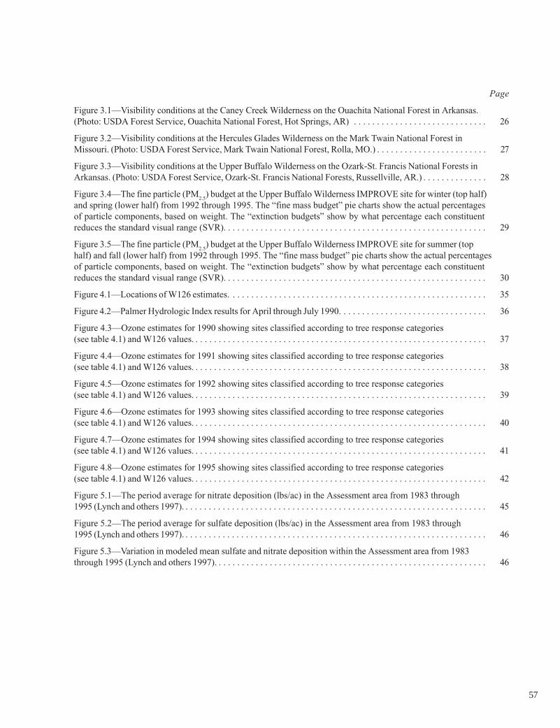
Page
Figure 3.1—Visibility conditions at the Caney Creek Wilderness on the Ouachita National Forest in Arkansas.(Photo: USDA Forest Service, Ouachita National Forest, Hot Springs, AR) . . . . . . . . . . . . . . . . . . . . . . . . . . . . . 26
Figure 3.2—Visibility conditions at the Hercules Glades Wilderness on the Mark Twain National Forest inMissouri. (Photo: USDA Forest Service, Mark Twain National Forest, Rolla, MO.) . . . . . . . . . . . . . . . . . . . . . . . . 27
Figure 3.3—Visibility conditions at the Upper Buffalo Wilderness on the Ozark-St. Francis National Forests inArkansas. (Photo: USDA Forest Service, Ozark-St. Francis National Forests, Russellville, AR.) . . . . . . . . . . . . . . 28
Figure 3.4—The fine particle (PM2.5
) budget at the Upper Buffalo Wilderness IMPROVE site for winter (top half)and spring (lower half) from 1992 through 1995. The “fine mass budget” pie charts show the actual percentagesof particle components, based on weight. The “extinction budgets” show by what percentage each constituentreduces the standard visual range (SVR). . . . . . . . . . . . . . . . . . . . . . . . . . . . . . . . . . . . . . . . . . . . . . . . . . . . . . . . . 29
Figure 3.5—The fine particle (PM2.5
) budget at the Upper Buffalo Wilderness IMPROVE site for summer (tophalf) and fall (lower half) from 1992 through 1995. The “fine mass budget” pie charts show the actual percentagesof particle components, based on weight. The “extinction budgets” show by what percentage each constituentreduces the standard visual range (SVR). . . . . . . . . . . . . . . . . . . . . . . . . . . . . . . . . . . . . . . . . . . . . . . . . . . . . . . . . 30
Figure 4.1—Locations of W126 estimates. . . . . . . . . . . . . . . . . . . . . . . . . . . . . . . . . . . . . . . . . . . . . . . . . . . . . . . . 35
Figure 4.2—Palmer Hydrologic Index results for April through July 1990. . . . . . . . . . . . . . . . . . . . . . . . . . . . . . . . 36
Figure 4.3—Ozone estimates for 1990 showing sites classified according to tree response categories(see table 4.1) and W126 values. . . . . . . . . . . . . . . . . . . . . . . . . . . . . . . . . . . . . . . . . . . . . . . . . . . . . . . . . . . . . . . . 37
Figure 4.4—Ozone estimates for 1991 showing sites classified according to tree response categories(see table 4.1) and W126 values. . . . . . . . . . . . . . . . . . . . . . . . . . . . . . . . . . . . . . . . . . . . . . . . . . . . . . . . . . . . . . . . 38
Figure 4.5—Ozone estimates for 1992 showing sites classified according to tree response categories(see table 4.1) and W126 values. . . . . . . . . . . . . . . . . . . . . . . . . . . . . . . . . . . . . . . . . . . . . . . . . . . . . . . . . . . . . . . . 39
Figure 4.6—Ozone estimates for 1993 showing sites classified according to tree response categories(see table 4.1) and W126 values. . . . . . . . . . . . . . . . . . . . . . . . . . . . . . . . . . . . . . . . . . . . . . . . . . . . . . . . . . . . . . . . 40
Figure 4.7—Ozone estimates for 1994 showing sites classified according to tree response categories(see table 4.1) and W126 values. . . . . . . . . . . . . . . . . . . . . . . . . . . . . . . . . . . . . . . . . . . . . . . . . . . . . . . . . . . . . . . . 41
Figure 4.8—Ozone estimates for 1995 showing sites classified according to tree response categories(see table 4.1) and W126 values. . . . . . . . . . . . . . . . . . . . . . . . . . . . . . . . . . . . . . . . . . . . . . . . . . . . . . . . . . . . . . . . 42
Figure 5.1—The period average for nitrate deposition (lbs/ac) in the Assessment area from 1983 through1995 (Lynch and others 1997). . . . . . . . . . . . . . . . . . . . . . . . . . . . . . . . . . . . . . . . . . . . . . . . . . . . . . . . . . . . . . . . . . 45
Figure 5.2—The period average for sulfate deposition (lbs/ac) in the Assessment area from 1983 through1995 (Lynch and others 1997). . . . . . . . . . . . . . . . . . . . . . . . . . . . . . . . . . . . . . . . . . . . . . . . . . . . . . . . . . . . . . . . . . 46
Figure 5.3—Variation in modeled mean sulfate and nitrate deposition within the Assessment area from 1983through 1995 (Lynch and others 1997). . . . . . . . . . . . . . . . . . . . . . . . . . . . . . . . . . . . . . . . . . . . . . . . . . . . . . . . . . . 46
57
U.S. Department of Agriculture, Forest Service. 1999. Ozark-Ouachita HighlandsAssessment: air quality. Report 2 of 5. Gen. Tech. Rep. SRS-32. Asheville, NC:U.S. Department of Agriculture, Forest Service, Southern Research Station. 57 p.
This publication provides information about the atmospheric conditions in and nearthe national forests in the Ozark-Ouachita Highlands: the Mark Twain in Missouri, theOuachita in Arkansas and Oklahoma, and the Ozark-St. Francis National Forests inArkansas. This report includes information about particulate matter, visibility, ozoneconcentrations, and acid deposition in the Ozark-Ouachita Highlands Assessment area.
Keywords: Acid deposition, Clean Air Act, ozone, particulate matter, pollution,visibility.
The Forest Service, U.S. Department of Agriculture, provides leadership in the manage-ment, protection, and use of the Nation’s forests and rangelands. The Agency takes anecological approach to the implementation of multiple-use management, providing
sustained yields of renewable resources such as water, forage, wildlife, wood, and recreation. TheForest Service has embraced ecosystem management as its operating philosophy and is committedto the preservation of wilderness, biodiversity, and landscape beauty as well as the protection ofthe basic resources of soil, water, and air quality.
The Forest Service is responsible for the 191.8-million-acre National Forest System, with its 155national forests and 20 grasslands in 44 States, Puerto Rico, and the Virgin Islands. In addition, theAgency works with State land management organizations to help private landowners apply goodnatural resource management practices on their lands. The International Program of the ForestService enables the Agency to share its technical expertise and managerial skills with other nations.The Research and Development Program of the Forest Service conducts extensive research toenhance and protect productivity on all of America’s forests and rangelands, with special attentionto long-term natural resource issues of national and international scope.
The U. S. Department of Agriculture (USDA) prohibits discrimination in all its programs andactivities on the basis of race, color, national origin, gender, religion, age, disability, political beliefs,sexual orientation, and marital or familial status. (Not all prohibited bases apply to all programs.)Persons with disabilities who require alternative means for communication of program information(Braille, large print, audiotape, etc.) should contact USDA’s TARGET Center at 202-720-2600 (voiceand TDD).
To file a complaint of discrimination, write USDA, Director, Office of Civil Rights, Room 326-W,Whitten Building, 14th and Independence Avenue, SW, Washington, DC 20250, or call 202-720-5964(voice or TDD). USDA is an equal employment opportunity provider and employer.

This report is one of five that documents the results of the Ozark-Ouachita HighlandsAssessment. Three of the remaining reports examine Aquatic Conditions, Social andEconomic Conditions, and Terrestrial Vegetation and Wildlife, respectively, and the fourthprovides an overall summary.
Summary Report
REPORT
1OF 5
Ozark-OuachitaHighlands Assessment
United StatesDepartment ofAgriculture
Forest Service
General TechnicalReport SRS-31 Aquatic Conditions
REPORT
3OF 5
Highlands AssessmentOzark-Ouachita
General TechnicalReport SRS-33
United StatesDepartment ofAgriculture
Forest Service
Terrestrial Vegetation and Wildlife
REPORT
5OF 5
Highlands AssessmentOzark-Ouachita
General TechnicalReport SRS-35
United StatesDepartment ofAgriculture
Forest Service
REPORT
4OF 5
Ozark-OuachitaHighlands Assessment
United StatesDepartment ofAgriculture
Forest Service
General TechnicalReport SRS-34 Social and Economic Conditions