United We Fight: National Unity and Interstate Conflict

By

Andrew Douglas Bertoli

A dissertation submitted in partial satisfaction of the

requirements for the degree of

Doctor of Philosophy

in

Political Science

in the

Graduate Division

of the

University of California, Berkeley

Committee in Charge:

Professor Ron Hassner, Co-chairProfessor Jasjeet Sekhon, Co-chair

Professor Thad DunningProfessor Aila MatanockProfessor Daniel Sargent

Summer 2016

Abstract

United We Fight: National United and Interstate Conflict

Andrew Douglas Bertoli

Doctor of Philosophy in Political Science

University of California, Berkeley

Professor Ron Hassner, Co-chair Professor Jasjeet Sekhon, Co-chair

Does unity within countries increase conflict between them? In this dissertation, I investigate whether it does using natural experiments. The first essay tests how exogenous surges of nationalism affect state aggression by exploiting a natural experiment that was created by the World Cup. The second essay analyzes whether united government increases state aggression by looking at a similar natural experiment. The third essay considers some of the methodological challenges that arose over the course of this project and draws lessons for future research. Along with shedding new light on the relationship between domestic unity and interstate conflict, this project demonstrates the value of using natural experiments to study international security.

1

Introduction

A central question in the study of international relations is how domestic unity affectsinterstate conflict. While national cohesion is generally viewed as having many benefits atthe domestic level, such as increasing government efficiency and economic growth, manyscholars worry that it can have a negative impact on international relations. These scholarsargue that two types of domestic unity are potentially dangerous. The first is social unity,or what is more commonly referred to as nationalism (Mearsheimer 1990). Among inter-national relations scholars, nationalism is widely viewed as a major source of internationalconflict, and researchers have linked it to state aggression using a wide range of method-ologies (Cederman, Warren, and Sornette 2011; Schrock-Jacobson 2012). The second isunited government, which occurs when one party controls the main bodies of government.Many international relations scholars believe that united government increases the likeli-hood of interstate conflict, since it gives leaders more freedom to take aggressive actionagainst other countries (Howell and Pevehouse 2005; Clark and Nordstrom 2006; Brulé2006).

Nonetheless, determining how domestic unity affects interstate conflict is very difficult.First, the relationship may be explained by reverse causality. That is, countries might be-come more united in the lead-up to international conflict, which could make it appear thatdomestic unity has a large effect on state aggression when it really does not. Second, therelationship could be driven by confounding factors. For example, the underlying politi-cal disputes could increase national unity in the lead-up to conflict, inducing a correlationbetween domestic unity and state aggression that is not actually causal.

In this dissertation, I attempt to overcome these problems by using regression disconti-nuity designs. Regression discontinuity is a type of natural experiment that takes advan-tage of scoring systems with important cut-points. The classic example is a test whereeveryone who scores above a 50% receives a scholarship and everyone who scores belowdoes not. If researchers wanted to analyze how winning the scholarship affected futureincome, they could compare the students who score 50’s to the students who score 49’s.The idea is that it should be nearly random which of them get the scholarship and whichdo not, so the data around the cut-point should be similar to experimental data.

The first paper in this dissertation uses a regression discontinuity involving the WorldCup to test how nationalism affects state aggression. Specifically, I compare countries thatbarely qualified for the World Cup to countries that barely missed. I find that World Cupparticipation increases the likelihood that countries will initiate military disputes againstother states. I also find that the countries that played against each other at that WorldCup were much more likely to have military conflicts afterward. These results underscorethe importance of being wary of other sources of nationalism, such as major national

1

achievements, tragedies, and revolutions. They also help legitimize concerns that the U.S.can provoke backlash by pursuing an activist grand strategy that foments nationalism inother countries.

The second paper in this dissertation tests how government unity affects state aggres-sion. Specifically, I look at close national elections where parties barely achieved or barelyfell short of united government. The results show that united government greatly increasesthe chances that democracies will initiate high-level disputes, and that it has no discernibleimpact on low-level disputes. The estimated effect is particularly large for the UnitedStates. These findings suggest that policymakers and the public should be alert to the po-tential danger of unnecessary conflicts when one party is in power. At the same time, theyshould be aware that divided governments might avoid some necessary conflicts, sinceopposition parties may wrongly oppose disputes where their countries should actually getinvolved. In short, believing that domestic politics “stop at the water’s edge” can increasethe chances that important foreign policy mistakes go unnoticed.

The third paper discusses some of the methodological challenges that arose over thecourse of this project and draws lessons for future research. The first issue discussedarises when units are grouped into different strata. For example, in the scholarship testscenario, students might be grouped in to classes of different sizes, with the top five stu-dents from each class getting the scholarship. This complication can threaten the validityof the design if not handled properly. The second issue involves units that appear in thesample multiple times, which would occur if students were allowed to retake the exam inthe test scholarship scenario. This issue can complicate the design, since some units wouldhave more than one score. The third issue arises when the treatment that researchers careabout is not actually assigned by the regression discontinuity. For example, a researchermight be interested in testing whether economic outcomes are better when Republicans orDemocrats win close elections, even though the ideology of politicians is not as-if random.Researchers can learn important lessons from these cases, but they need to be careful whenanalyzing this type of design.

While these projects shed light on important substantive and methodological questions,they also demonstrate the promise of using natural experiments to study international con-flict. The design-based inference movement that has led to breakthroughs in American andcomparative politics is still just gaining traction in IR, due to the difficulty of studying ma-jor questions in international relations with natural experiments. This dissertation showshow important international relations topics can be addressed with design-based methods.

2

REFERENCES

Brulé, David. 2006. “Congressional Opposition, the Economy, and US Dispute Initiation,1946-2000.” Journal of Conflict Resolution 50(4): 463-483.

Cederman, Lars-Erik, T. Camber Warren and Didier Sornette. 2011. “Testing Clausewitz:Nationalism, Mass Mobilization, and the Severity of War.” International Organization65(4), 605-38.

Clark, David H. 2000. “Agreeing to disagree: Domestic institutional congruence and USdispute behavior.” Political Research Quarterly 53(2): 375-400.

Mearsheimer, John. 1990. “Why We Will Soon Miss the Cold War.” The Atlantic Monthly266(2), 35-50.

Howell, William G. and Jon C. Pevehouse. 2005. “Presidents, Congress, and the Use ofForce.” International Organization 59(1): 209-232.

Schrock-Jacobson, Gretchen. 2012. “The Violent Consequences of the Nation: National-ism and the Initiation of Interstate War.” Journal of Conflict Resolution 56(5), 825-52.

3

Nationalism and Interstate Conflict:A Regression Discontinuity Analysis

Andrew Bertoli

27 March 2016

ABSTRACT. Does nationalism make interstate conflict much more likely, or are its effectslargely constrained by strategic realities? This question matters for how scholars thinkand theorize about international relations, but answering it has been difficult because ofendogeneity and measurement issues. To overcome these problems, I look to one of themost powerful sources of nationalism in the modern era–international sports. I begin byinvestigating several cases where surges of nationalism from sporting events led to militaryor political conflict between countries. I then analyze a regression discontinuity that wascreated by the format of the World Cup qualification process from 1958-2010. The resultsprovide strong evidence that World Cup participation increases state aggression, especiallyfor countries where soccer is the most popular sport. I also show that nationalism bestexplains these results by investigating two cases from the dataset and considering someadditional evidence.

Scholars use nationalism to explain international conflicts from the Napoleonic Warsto the U.S. invasion of Iraq following September 11 (Rosato 2003; McCartney 2004; Ce-derman, Warren, and Sornette 2011). In fact, nationalism is one of the few factors thatinternational relations theorists across paradigms view as an important force for interstateviolence (Mearsheimer 1990; Wendt 1999; Keohane and Nye 2001). Scholars argue that itcan increase enmity between countries (Walt 2011), undermine international cooperation(Rosato 2011), motivate societies to fight costly wars (Posen 1993), and cause govern-ments to overestimate their relative military power (Snyder 2000). Moreover, many the-ories of war are premised on the idea that nationalism is an important source of conflict.Some examples include the theory that war can result from surges of nationalism follow-ing revolutions (Snyder and Mansfield 1995) and the theory that charismatic leaders whomanipulate national sentiments make conflict more likely (Byman and Pollack 2001).

Nevertheless, whether fluctuations in nationalism can actually have a causal impacton interstate violence is a question that has thus far remained unanswered (Posen 1993;Schrock-Jacobson 2012). One concern is that national identities are already so salient thatadditional increases in nationalism may have a very small effect on the likelihood of war.Another is that surges of nationalism might make little difference given the constraints

4

imposed on states by the international system. Past studies that have sought to address thisquestion have faced two major challenges. First, there is no comprehensive dataset thattracks nationalism across the international system, or even an established way to measureit in any given case. Second, even though nationalism often appears to increase in thelead-up to war, it is very difficult to show that this relationship is causal. For instance, theexisting political disputes underlying the conflict might create the nationalism, or leadersmight try to incite it to increase morale for a future war (Posen 1993).

This paper tests how fluctuations in nationalism influence state aggression by lookingat surges of nationalism that were created by international sports. Sporting events are anideal place to look because it is widely accepted that they increase the salience of nationalidentities. Scholars have shown that they often lead to feelings of national unity and hatredtowards other countries (Vincent et al. 2010). These sentiments have resulted in frequentoutbreaks of nationalistic violence at games (Markovits and Rensmann 2010), and at timeshave intensified rivalries at the international level (Reid 1999; Hitchens 2010; Schama2014). Some famous examples include the 1969 Football War between El Salvador andHonduras, the 2009 Egypt-Algeria World Cup Dispute, the 1936 Nazi Olympics, and thecontroversial Moscow Dynamo soccer club trip to Britain in 1945 (Orwell 1945; Lindsey2009).

To overcome the endogeneity problem, I analyze a regression discontinuity that wascreated by the format of the World Cup qualification process from 1958-2010. Over thisperiod, many countries qualified for the World Cup by playing a round of games againstother states and achieving a top position in the final standings. It is therefore possibleto compare the group of countries that barely qualified to the group that barely missed.These countries went to the World Cup or stayed home based on small differences in theirrecords after many games, so the data obtained by this procedure should be similar to whatwould be expected in a randomized experiment.

Using this approach, I construct a sample of countries that barely qualified or barelymissed the World Cup. Specifically, I select pairs of countries where one country qualifiedand the other fell short, provided that they were separated by no more than two points inthe standings and the qualifier scored at least five points. I made these design choices priorto collecting the data, believing that they would lead to a sufficiently large sample underwhich qualification was as-if random. In total, the sample consists of 142 countries, with71 barely qualifying and 71 barely missing. The qualifiers and non-qualifiers are balancedacross a wide range of political, economic, and demographic factors, which supports theas-if random assumption. They are also balanced on past levels of aggression, which Imeasure in the standard way as the number of militarized interstate disputes that a countryinitiates.

The results show that going to the World Cup increases aggression substantially. Thecountries that barely qualified experienced a significant spike in aggression during theWorld Cup year. The disputes that they started also tended to be much more violent

5

than the disputes started by the non-qualifiers. The results hold under various robust-ness checks, and the estimated treatment effect is much higher for countries where socceris the most popular sport. Substantively, the estimates suggest that going to the World Cupincreases state aggression by about two-fifths as much as a revolution does, and that it hasroughly the same effect as electing a leader who is backed by the military.

It is also possible to replicate the analysis using the FIFA regional soccer championshipslike the European Football Championship and the African Cup of Nations. In total, thisnew sample consists of 78 countries that barely made or barely missed their regional soc-cer tournaments. The qualifiers and non-qualifiers were again well-balanced on aggressionlevels prior to qualification, but the qualifiers became significantly more aggressive follow-ing qualification. The results from this analysis are available in the Online Appendix.

This paper proceeds as follows: I first review the existing theoretical and empirical workabout the relationship between nationalism and war. I then elaborate on why internationalsports provide an excellent opportunity to test whether exogenous surges of nationalismhave a major causal impact on state aggression. Next, I examine some qualitative evidencefrom the history of international sports that suggests that nationalism can lead to conflict onthe international stage, and I consider some of the mechanisms through which this processcan unfold. I then explain my research design in more depth and present the results fromthe World Cup analysis. After that, I explore two cases from the dataset and perform someadditional tests. The final section concludes.

SECTION 1: EXISTING LITERATURE ON NATIONALISM AND WAR

Nationalism is generally defined as the practice of identifying with a nation-state andviewing other nations as competitors that are culturally or morally inferior (Orwell 1945).For many, this identification is so powerful that it compels them to kill and die for theircountries (Rosato 2003). While this devotion may be somewhat difficult to explain at theindividual level, most scholars agree that it is a wide-spread phenomenon (Anderson 1983;Robinson 2014), and that it plays a central role in international relations (Mearsheimer1990; Wendt 1999). Most importantly, it defines the boundaries of the international systemthat scholars often take for granted. It also helps explain how major war between countriesis possible by ensuring that there will be people who are willing to die for the nationalinterest.

Nevertheless, there is much less certainty about whether surges of nationalism have animportant causal impact on state behavior. The effects of nationalism might be greatlyconstrained by strategic factors, or nationalism might not fluctuate enough to have notice-able effects at the international level. A central problem in answering this question hasbeen endogeneity. As Posen (1993) explains, “Leaders use nationalism to mobilize publicsupport for military preparation and sacrifices. When war seems imminent, for any reason,the intensity of propaganda increases. The same is true when wars last for any length of

6

time. Thus it will often be difficult to show that nationalism caused any conflict, becauseit will generally be accompanied and accentuated by other causes of the conflict.”

But despite this concern, many international relations scholars believe that nationalismhas been an important source of conflict throughout history. For instance, they have usedit to explain the conquests of Imperial Germany and Japan, the breakup of the SovietUnion, and the Balkans Wars (Mearsheimer 1990; Snyder and Mansfield 1995; Van Evera1994). The view that nationalism can be a force for conflict also underpins many importantarguments made by international relations scholars, like that bombing civilians duringwartime makes the target population less willing to surrender (Pape 1996) and that theUnited States can provoke backlash by stationing military troops abroad (Posen 2013).No doubt, the idea that nationalism can cause interstate violence influences how manyscholars think about international relations.

Moreover, many theories of war are predicated on the idea that high levels of national-ism make conflict more likely. For instance, this idea is central to the theory that emergingdemocracies are likely to start wars as a result of the hypernationalistic rhetoric of theirleaders who seek to increase their domestic support (Snyder and Mansfield 1995; Snyder2000). Similarly, this idea underpins the theory that war can be caused by charismaticleaders who have the ability to rally mass nationalism (Byman and Pollack 2001). It isalso key to theories that focus on variation in nationalism across the international system.For example, the idea that grievances from past wars or atrocities can explain why somenations fight each other is based on the idea that the intensity of nationalism can have animportant impact on the likelihood of conflict (Van Evera 1994).

In short, knowing the extent to which nationalism affects state aggression matters forhow scholars think and theorize about international relations. While past quantitative ef-forts to investigate this question have remained limited, in part because there is no compre-hensive dataset that tracks nationalism, a number of recent studies have made noteworthyprogress. First, several experiments have found that people tend to think more hawkishlywhen they see their national flags (Hassin 2007; Kemmelmeier and Winter 2008). Thesestudies provide important micro-level evidence of a causal link between nationalism andconflict. However, they fall short of showing that nationalism affects state behavior, be-cause they only look at the responses of individuals.

Second, Schrock-Jacobson (2012) recently provided a major contribution to this re-search program by conducting the first large-N cross-national study that tests the rela-tionship between nationalism and military conflict directly. To deal with the measure-ment problem, she selected a random sample of state-years from 1816-1997 and coded forwhether countries experienced a nationalistic movement in those years. Using regression,she shows that there is a correlation between nationalism and the onset of war that does notdisappear after controlling for some baseline factors. While this result provides valuableobservational evidence for a causal relationship between nationalism and conflict, it may

7

be explained by omitted variable bias. This problem is concerning because countries usu-ally become more nationalistic in the lead-up to war, and the anticipation of future conflictis a difficult variable to observe or proxy.

Thus, measurement and endogeneity issues have made it difficult to test whether surgesof nationalism can have an important impact on interstate violence. In the next section, Ipropose a new strategy to overcome these challenges.

SECTION 2: USING INTERNATIONAL SPORTS AS A SOURCE OF NATIONALISM

International sports provide an excellent opportunity to test whether nationalism hasa causal effect on interstate conflict. First, they offer a way around the measurementproblem. While past studies have struggled to find a reliable, comprehensive measureof nationalism that spans across countries and time, most political scientists agree thatinternational sporting events increase it (Cha 2009; Markovits and Rensmann 2010; Walt2011). Sociologists have also shown that international sports often make the nationaldiscourses within countries more hawkish, with reporters describing games in militaryterminology and comparing wins and losses to past battles (Garland and Rowe 1999). AsVincent (2010) explains, “only warfare feeds the imagination and cements national identitymore than sports.”

There are many examples where international sports have increased national unity withincountries. One of the most famous cases was Nelson Mandela’s use of rugby to unite SouthAfrica following the end of the apartheid regime (Steenveld and Strelitz 1998). Similarly,qualification for the 2006 World Cup helped unify the Ivory Coast after four years of civilwar (Mehler 2008). Government leaders in Yemen also used the national soccer team tohelp break down divisions between the northern and southern regions of the country fol-lowing integration in 1990 (Cha 2009). In short, international sports can evoke feelings ofnationalism that spill over into the political realm.

A second advantage is that it is very hard to imagine how sports could increase thechances of interstate conflict in any way besides generating nationalism. The most plau-sible alternative explanation may be that sports distract the public, giving leaders morefreedom to do what they want on the international stage. However, this mechanism wouldonly explain a very short term effect, which is inconsistent with the data that I presentlater in this paper. Other possibilities that are unrelated to nationalism are hard to thinkof, in part because international sports and nationalism are inextricably linked. The vastmajority of fans root for their countries because of national identification, and the very actof cheering for one’s side is an expression of nationalism (Hobsbawm 1990).

A third major advantage of using international sports is that the most popular sportingevent, the World Cup, created a regression discontinuity where surges of nationalism wereessentially exogenous. As I will discuss more in the coming sections, qualification for the

8

World Cup was as-if random for a large number countries. This natural experiment allowsus to avoid the endogeneity problem that has left past research somewhat inconclusive.

There are also many historical cases that suggest that international sports increase thechances of interstate violence by inciting nationalism, so it is plausible that this designcould work. I will turn to these cases in the next section to provide some preliminaryqualitative evidence that nationalism from sporting events can increase state aggressionand to consider some of the ways that this process can occur.

SECTION 3: INVESTIGATING THE HISTORICAL EVIDENCE

The idea that nationalism from sporting events can increase the likelihood of interstateconflict has been advanced by many writers (Orwell 1945; Reid 2000; Hitchens 2010;Markovits and Rensmann 2010; Schama 2014). These scholars have identified a numberof cases where nationalism from sporting events appears to have led to major militaryor political conflict between countries. Their research suggests that conflict is often theunintended consequence of sports nationalism, but that leaders also sometimes exploitinternational sporting events to generate support for their foreign policy ambitions. Ineither case, mass nationalism increases leaders’ opportunity and incentive to go on theoffensive. I discuss these cases below, and then I conclude by highlighting some importantpoints to note from history.

1969 Football War. Many studies have concluded that this war was caused by a seriesof soccer riots that exacerbated an already tense political situation between El Salvadorand Honduras (Anderson 1981; Reid 2000; Kapuscinski 2013). In the late 1960s, theHonduran government began taking land from the Salvadoran immigrants living in itscountry and giving it to Honduran-born peasants in response to unrest among Honduranagricultural workers. This policy led to skirmishes between Honduran and Salvadorannationals and prompted a media war between the two countries that further encouragedxenophobia.

In this volatile political atmosphere, Honduras and El Salvador played three World Cupqualification games. The night before the first game in Honduras, a mob of Honduranssurrounded the hotel where the Salvadoran players were staying and made as much noiseas possible to prevent them from sleeping. The next day, El Salvador lost 1-0, but storiesof the incident were widely reported throughout El Salvador and incited public outrage.When the Honduran team traveled to El Salvador to play the next game, Salvadoran fansthrew rocks through the windows of the hotel where the Honduran players were stayingand used drums, horns, and bands to keep the team up all night. The crowd was so hostilethat the next morning the Honduran players had to be driven to and from the stadiumin armored cars, and the Salvadoran army was needed to provide security at the game.Outside the stadium, Salvadoran fans assaulted many Hondurans, burned their cars, and insome cases chased them to the border. Honduras lost the game 3-0.

9

When news of what happened reached Honduras, it prompted widespread violenceagainst Salvadoran nationals living in the country, and thousands were forced to flee toEl Salvador. Tensions escalated again when the countries played a tie-breaking game thir-teen days later in Mexico City that needed to be supervised by the Mexican military. Thatday, the two sides broke diplomatic ties and El Salvador formally accused the Hondurangovernment of human rights violations for not protecting the Salvadoran nationals livingin its country. Less than three weeks later, El Salvador invaded Honduras, starting a warthat caused about two thousand casualties (Reid 2000).

2009 Egyptian-Algerian World Cup Dispute. This conflict began after Egyptian fans at-tacked a bus transporting the Algerian team and injured three players. Algerians retaliatedagainst Egyptian companies and property in Algeria. In response, Mubarak removed theEgyptian ambassador from Algiers, gave an impassioned speech about Egypt’s insultednational pride, and accused the Algerian government of staging the attacks on its players(Lindsey 2009). Egypt also sent a plane into Algeria to rescue Egyptian nationals from thesoccer violence, although the aircraft was not granted permission to land (Shenker 2009).As Hitchens (2010) describes, “Before the match in Khartoum, Egypt and Algeria hadno diplomatic quarrel. After the game, perfectly serious people in Cairo were saying theatmosphere resembled that following the country’s defeat in the June 1967 war.” In fact,the Arab League responded to this incident by proposing that politicians from its memberstates should not attend sensitive sports games because these events could make them morehostile toward other countries (Belmary 2009).

2014 Serbian-Albanian Drone Conflict. Serbian and Albanian soccer fans have a historythat is so marred with violence that they are not allowed to attend each other’s games. Ata UEFA Cup qualifying game in Serbia on October 14, 2014, Albanian fans flew a smalldrone into the stadium that was carrying an Albanian flag. When the drone got closeenough to the ground, a Serbian player ripped the flag off, sparking a fight between theSerbian and Albanian teams. Serbian fans rushed the field to attack the Albanian players,who were barely able to get back to their locker room.1 Serbia called the drone stuntan “act of terrorism” designed to provoke Serbian fans and claimed that the brother ofthe Albanian president was behind it (Riach 2014). Albania accused Serbian police ofattacking Albanian players.

1934 Italian World Cup. Throughout the 1930s, Mussolini intentionally used sports toincrease support for the Italian war machine. As Tunis (1936) describes, the main pur-pose of sports for Mussolini was “the mass production of cannon fodder.” He writes,“sport ceased to be a free activity and became a function of the government... The resultsare watched, collected, catalogued and exploited, at home and abroad.” Similarly, Martin

1. A video of this incident is available at http://www.tubechop.com/watch/6035427.

10

Table 1 Notable Cases Where Scholars Have Claimed ThatSports Nationalism Led to Interstate Conflict

1. Football War (1969)2. Egypt-Algeria World Cup Dispute (2009)3. Serbia-Albania Drone Conflict (2014)4. Italian World Cup (1934)5. Nazi Olympics (1936)6. Bodyline (1932)7. Moscow Dynamo Soccer Trip to Britain (1945)8. Croatian War of Independence (1991)

(2004) explains that the 1934 World Cup “was more like a fascist rally than a sporting con-test.” Goldblatt (2008) draws a clear link between this competition and Italian aggressiontoward other countries. As he describes, “The preparations for the tournament coincidedwith a steadily more expansionist and aggressive foreign policy that would culminate afterthe World Cup in the invasion of Abyssinia (Ethiopia), intervention in the Spanish CivilWar and relentless pressure on Albania and Central Europe.”

1936 Nazi Olympics. Following Mussolini’s example, Hitler used the 1936 Nazi Olympicsto provoke feelings of Aryan supremacy and victimization in Germany during the lead-upto World War II (Rippon 2006). Large (2007) describes the games as “a crucial part of theNazi regime’s ‘spiritual mobilization’ to win the hearts and minds of the German people,”and Schama (2014) argues that they played a pivotal role in creating domestic support forGerman expansion. In fact, Hitler did not care about sports until his advisers convincedhim that they could be used to generate support for the German war machine (Krüger1998). Of course, these scholars are not suggesting that World War II would not havehappened without the 1936 Olympics, but the case illustrates how leaders with militaryambitions can use nationalism from sports to increase public support for aggression.

Other Cases. Table 1 lists the examples discussed above along with some other notablecases where scholars have argued that nationalism from sporting events led to major mili-tary or political conflict between countries. Bodyline (1932) was a dispute between Britainand Australia over cricket that resulted in rioting, nationalistic vandalism, boycotts, andother economic fallout. Many Australians consider Bodyline to be one of the two mainreasons that Anglo-Australian relations collapsed in the 1930s, with the other being theGreat Depression (Frith 2013; Swan 2013). The Moscow Dynamo soccer trip to Britain

11

(1945) involved a series of games that were supposed to help strengthen relations betweenBritain and the Soviet Union following World War II. However, they led to fights and nu-merous controversies over cheating, and Britain canceled the tour early when it becameclear that the Soviets were exploiting the games to generate nationalism at home (Orwell1945; Kowalski and Porter 1997). I also include the Croatian War of Independence as acase because it was prefaced by a substantial amount of soccer violence. In fact, manySerbs and Croats consider a battle in the Croatian soccer stadium to be the unofficial be-ginning of the war (Ðordevic 2009). While there were major underlying political disputesat the time, Sack and Suster (2000) argue that “it would be a mistake to view these matchesas mere epiphenomena mirroring larger social and political events but having no power toinfluence them.”

Key Points. These cases illustrate three key points about conflicts from internationalsporting events:

(1) The nationalism can be unintended or driven by government leaders. In manycases, especially the Football War and Bodyline, international tension arose simply fromthe passions that sports evoke. Emotions over the sporting event changed public opinion,and leaders then had to respond. However, in other cases, most notably the 1934 WorldCup and the 1936 Olympics, leaders deliberately exploited international sports to generatepublic support for their aggressive foreign policy agendas. The sporting event gave thema way to create a surge of nationalism in their country that could change public opinion.Thus, these cases suggest that nationalistic conflict may be accidental or elite-driven. Bothcausal paths appear to be valid ways that nationalism can intensify international rivalry.

(2) The conflict is sometimes between countries that compete against each other head-to-head, but not always. As the 1934 World Cup and the 1936 Olympics demonstrate,nationalism from sporting events can increase the likelihood of conflict between coun-tries even when they do not play against each other directly. Ethoipia did not attend the1934 World Cup, but it was the first target of Italian expansion in 1935. Similarly, theSoviet Union and Jewish community boycotted the 1936 Olympics, although they foundthemselves the victims of German nationalism in the coming years. This idea that sportsnationalism can lead to conflict indirectly is also supported by Iraq’s experience at the2007 Asian Cup, which Stephens (2007) claims increased Iraqi nationalism and feelingsof resentment toward the United States. Similarly, when countries play games againststates that they do not have an international rivalry with, it is common for their fans toburn flags of their traditional rival countries.

This distinction between the direct and indirect effects of sports nationalism is importantbecause the main test in this paper focuses on the indirect effect. Since countries playonly a few other states at the World Cup, most of whom are far away geographically,the test in this paper primarily relies on indirect conflicts. Thus, it investigates whether

12

state aggression can increase from general nationalism (like in the case of the FrenchRevolution), rather than from nationalism that is directed at a specific rival country (likein the case of the Football War). However, I also show in the results section that the pairsof countries that played against each other at the World Cup became much more likely toengage in military disputes afterward.

(3) Nationalism from sports appears capable of having downstream effects. In caseslike the 1934 World Cup and Croatian War of Independence, tension from sports did notimmediately translate into conflict at the international level. Rather, it appears to haveprimed people to think more aggressively towards other countries, thereby influencingtheir behavior when disputes did arise in the future. The analog case in U.S. history mightbe how nationalism from September 11 made many Americans much more willing toinvade Iraq over a year-and-a-half later (McCartney 2004). Thus, we should expect thatthe World Cup may have downstream effects that appear a year or two afterward.

SECTION 4: DESIGN

Strategy for Identifying the Causal Effect. I estimate the impact of World Cup partic-ipation on state aggression by using a regression discontinuity design. This method hasbecome an increasingly popular research technique in the social sciences over the lastdecade for its ability to identify causal effects (Dunning 2012). It can be used when atreatment is given to units that surpass a certain cut-point in a scoring system. The ideais to compare the group of units that scored just above the cut-point to the group thatscored just below it. For example, if there was a test where everyone who scored a 50%or higher received a scholarship, we could assess the impact of winning the scholarship bycomparing people who scored 50% to people who scored 49%. As long as there is somerandomness in the scoring process, it should be close to random who ended up on eitherside of the cut-point (Lee 2008). Thus, this method should produce the type of data thatwe would expect in a randomized experiment.

There are two main approaches to analyzing regression discontinuities. The first is tocompare the units that scored just above the cut-point to units that scored just below itusing normal experimental tests (Dunning 2012; Cattaneo, Frandsen, and Titiunik 2015).The advantage of this approach is that it makes very few statistical assumptions, since it isessentially a natural experiment with a quasi-random treatment. The major decision thatresearchers must make is how to define barely making and barely missing the treatment.In the test example, researchers might look at the students who scored 49% and 50%, orthey might also want to include students who scored 48% and 51%.

The second approach is to estimate the difference in the potential outcomes at the cut-point using two regression lines (Voeten 2013). This approach does not assume as-if ran-domness in a small window around the cut-point. Instead, it requires that the potential

13

outcomes are smooth in an area around the cut-point and that they can be estimated rea-sonably well using regression. Researchers using this approach must make a number ofdecisions, including which smoother and bandwidth selection procedure to use and howto estimate the confidence intervals for the regression lines.

My results are significant for both approaches, although I focus on the first approach inthis paper. The main reason is that the standard procedures for the second approach arenot valid when dealing with a scoring system that has discrete values, such as the WorldCup qualification process (Lee and Card 2008; Cattaneo, Frandsen, and Titiunik 2015). Inaddition, the first approach is more intuitive and requires less design choices. It also doesnot depend on regression predictions at the cut-point, which may be unreliable since thecut-point is an endpoint for both regression lines.

To address the fact that which countries barely qualify and barely miss is not perfectlyrandom, I use a difference-in-differences estimator to reduce any possible bias. Thus, Icompare the change in aggression for the countries that barely qualified to the change inaggression for the countries that barely missed. As a robustness check, I also control forbaseline differences between the qualifier and non-qualifier groups using linear regression.The findings remain significant under all specifications, which are primarily detailed in thesupporting information. I also show that the results are insensitive to the limited numberof design choices that I made, such as how I defined the bare qualifiers and bare non-qualifiers. I explain these choices in the next section.

Constructing the Treatment and Control Groups. The World Cup takes place once ev-ery four years during the summer, with the qualification process ending the winter before.The first qualification round was held in 1934, and it has been in place ever since. Thehost country qualifies automatically, as did the winner of the previous World Cup up until2010. All other countries are required to play their way in. They do so in one of two ways:(1) by playing a round of games against other states in their region and earning a certainposition in the standings or (2) by winning a play-in game or several playoff games. Eitherway, the format is set well in advance.

This study focuses on the standings format, which is illustrated in Table 2.2 In thestandings format, countries that were very close to the qualification cut-point went to theWorld Cup or stayed home based on small differences in their records after many games.Thus, qualification should be close to random for these countries. This as-if randomnessshould make the group of states that barely qualified similar to the group that barely missedacross observable and unobservable factors. Moreover, we can check that the qualifiers andnon-qualifiers are balanced to verify that the design worked.

The playoff format is less easy to exploit with regression discontinuity analysis. Coun-tries make or miss the World Cup based on their performance in the final round, which

2. Before 1994, countries earned two points for a win, one point for a tie, and nothing for a loss. Startingin 1994, the value of a win was increased to three points.

14

Table 2 Example of the Final Standings from a 1994Qualification Round

Rank Country Score Qualified1 Italy 16 Yes2 Switzerland 15 Yes3 Portugal 14 No4 Scotland 11 No5 Malta 4 No6 Estonia 1 No

Note: The sample consists of pairs of countries like Switzerland andPortugal that barely made and barely missed qualification.

could be correlated with other factors that are related to their likelihood of future aggres-sion. This problem is particularly concerning because the last game in the playoff formatis often played between countries from different regions that have large disparities in termsof GDP and population, along with many other factors. However, the findings in this studyremain significant when close playoff games are included, so the results are not sensitiveto whether the outcomes of these games are considered random or not.

Using data from the standings format from 1934-2010, I select pairs of countries thatwere separated by no more than two points in the standings, provided that the winnerscored at least five points. In total, the sample consists of 142 countries, which are listedin Table 3. There were seven pairs before 1958 where the winner scored less than fivepoints. In these cases, the teams played only a small number games, typically three or lesseach. Since the goal of the design was to obtain two groups of countries that were assignedto treatment or control based on small differences in their records after many games, thesecountries were dropped from the analysis.

Seventeen of the 71 pairs tied in the standings. Nine of these ties were broken by aplayoff game, seven were decided by looking at which country had the larger averagemargin of victory, and one was decided by which team scored more goals. I include thesepairs in the analysis for two reasons. First, the playoff games were more like toss-upsbecause they were played between teams of comparable skill. Second, there are not strongreasons to believe that comparable teams would sort based on margin of victory or totalgoals scored. Nevertheless, the results remain significant whether ties are included or not.

Lastly, I had to remove pairs where one of the teams did not represent a country. Iexclude Scotland, Northern Ireland, and Wales from this analysis, and I count Englandas Britain. I also exclude the Representation of Czechs and Slovaks, which was a union

15

Table 3 Countries That Barely Made and Barely Missed the World CupQualifier Non-qualifier Year Qualifier Non-qualifier Year

Yugoslavia Romania 1958 Tunisia Egypt 1978France Belgium 1958 France Ireland 1982Austria Netherlands 1958 Austria Bulgaria 1982

Soviet Union Poland 1958 Britain Romania 1982Hungary Bulgaria 1958 Peru Uruguay 1982Britain Ireland 1958 El Salvador Mexico 1982

Paraguay Uruguay 1958 New Zealand China 1982Argentina Bolivia 1958 Portugal Sweden 1986Bulgaria France 1962 Soviet Union Switzerland 1986

Switzerland Sweden 1962 Bulgaria East Germany 1986Portugal Czechoslovakia 1966 Romania Denmark 1990Bulgaria Belgium 1966 Austria Turkey 1990

West Germany Sweden 1966 Czechoslovakia Portugal 1990Chile Ecuador 1966 United States Trinidad 1990

Czechoslovakia Hungary 1970 UAE Qatar 1990Romania Greece 1970 Ireland Denmark 1994Bulgaria Poland 1970 Switzerland Portugal 1994

Italy East Germany 1970 Bulgaria France 1994Sweden France 1970 Netherlands Britain 1994Belgium Yugoslavia 1970 Bolivia Uruguay 1994

Peru Bolivia 1970 Cameroon Zimbabwe 1994Morocco Nigeria 1970 Nigeria Ivory Coast 1994Sweden Austria 1974 Morocco Zambia 1994

Netherlands Belgium 1974 South Korea Japan 1994Yugoslavia Spain 1974 Nigeria Guinea 1998

East Germany Romania 1974 Jamaica Costa Rica 1998Poland Britain 1974 Chile Peru 1998

Uruguay Colombia 1974 Senegal Morocco 2002Argentina Paraguay 1974 Nigeria Liberia 2002

Haiti Trinidad 1974 Ivory Coast Cameroon 2006Italy Britain 1978 Tunisia Morocco 2006

Austria East Germany 1978 Togo Senegal 2006France Bulgaria 1978 Angola Nigeria 2006Poland Portugal 1978 Algeria Egypt 2010Sweden Norway 1978 Nigeria Tunisia 2010Spain Romania 1978

16

of players from the Czech Republic and Slovakia that played from 1992-93. No otherchanges were necessary.

Measuring Aggression. Similar to past studies (Lai and Slater 2006; Colgan 2010), Imeasure aggression using the number of militarized interstate disputes (MIDs) that a coun-try initiates. These disputes are instances where states explicitly threaten, display, or useforce against other countries (Ghosn, Palmer, Bremer 2004). This measure is commonlyused in security studies, since wars happen too infrequently to be a useful measure in moststatistical tests. While most MIDs are low-level and not very interesting in their own right,they are a good proxy for the likelihood of major interstate conflict. They are indicativeof the foreign policy stance of a country and whether that country is willing to initiateconflicts with its rivals. I also show in the next section that the results remain significantfor high-level disputes that involved a direct attack, clash, or the start of interstate war.

Checking for Balance. The goal of the design was to achieve balance across observableand unobservable pre-treatment characteristics. The qualifier and non-qualifier groupsshould be similar except that the qualifiers went to the World Cup and the non-qualifiersdid not.

Of course, we should not expect the two groups to look exactly the same on pre-treatment factors. There will be some baseline differences simply by chance. In ran-domized experiments, the p-values for pre-treatment characteristics should be distributeduniformly between 0 and 1. Thus, there are statistically significant differences at the 5%level for about one out of every 20 pre-treatment characteristics, simply because of chancevariation. But the inferences drawn from this study will be most credible if the quali-fiers and non-qualifiers are balanced on all observable characteristics that might influencefuture aggression, as well as on past levels of aggression.

Figure 1 provides a comparison between the two groups. Since the qualification roundends about six months prior to the summer of the World Cup, the data used in this summarywere taken from the year before the World Cup. The qualification rounds finished at theend of this year. For each variable, I plot the p-value from a two-tailed paired t-test thatevaluates the difference in means between the qualifier and non-qualifier groups. I alsoplot the p-values for aggression levels in the years leading up to the World Cup.

Overall, the balance between the qualifiers and non-qualifiers looks similar to whatwould be expected in a randomized experiment. The p-values seem to be distributed uni-formly between 0 and 1, which supports the idea that this data is like experimental data.Most importantly, the qualifiers and non-qualifiers are balanced on levels of aggression inthe years leading up to the World Cup. In fact, this comparability extends much furtherback. If you compare the aggression levels of the qualifiers and non-qualifiers in eachof the 50 years prior to qualification, there is statistical significance only twice at the 5%level, in Year -10 and Year -36. Aside from these years, the difference in aggression levelsbetween the two groups is never significant at even the 10% level. The p-value over the

17

Figure 1 Balance Between the Qualifiers and Non-Qualifiers

VariableName

TreatmentMean

ControlMean

Total Population 33,438,500 35,742,500Urban Population 9,189,200 8,879,540

Imports 23,614,700,000 18,628,100,000Exports 21,695,600,000 18,894,900,000

Material Power Score 0.01 0.009Level of Democracy 0.465 0.465

Engaged in Civil War 0.01 0.01Resolved Civil War 0.01 0

Year of State Formation 1881 1877Birth Rate 23.6 24

Infant Mortality 51.1 50.6Life Expectancy 65.6 66

Median Age 27.7 27.7Number of Alliances 15.7 16.5

U.S. Ally 0.4 0.479Soccer Most Popular Sport 0.93 0.93

Appearance at Previous World Cup 0.352 0.31MIDs Initiated in the Year Before 0.183 0.113

MIDs Initiated in the 3 Years Before 0.69 0.577MIDs Initiated in the 5 Years Before 1.07 0.873

0 .05 .1 1

p−value

entire 50-year period is p = 0.46, with the qualifiers averaging 0.04 disputes per year morethan the non-qualifiers.

Thus, the data passes an important placebo test. It is unlikely that the balance plotleft out some factor that would make the qualifiers significantly more aggressive than thenon-qualifiers after qualification, since this factor should have also made the qualifiersmuch more aggressive before qualification. So aside from the treatment effect, there islittle reason to suspect that the qualifiers would behave much more aggressively than thenon-qualifiers after qualification.

SECTION 5: FINDINGS

Although the qualifiers and non-qualifiers were comparable on past levels of aggression,the story is much different following qualification. Figure 2 tracks the aggression levelsof the two groups over this period. Prior to qualification, they had very similar records

18

Figure 2 Comparing Aggression Before and After the World Cup

Qua

lific

atio

nW

orld

Cup

__Qualifiers

Non−qualifiers

0

5

10

15

−5 −4 −3 −2 −1 1 2 3 4Years Since Qualification and the World Cup

Milit

arize

d In

ters

tate

Dis

pute

s In

itiat

ed

of aggression. However, the qualifiers became much more aggressive following qualifi-cation, and they remained so until about the second year after the tournament. The factthat the increase in aggression begins after qualification is consistent with historical evi-dence showing that many countries experience a surge of nationalism when their countriesqualify for the World Cup (Ralph 2007; Mehler 2008).

Note that the aggression levels of the two groups drop the year before qualification, andthen the qualifiers spike while the non-qualifiers stay low. This trend is consistent withthe theory that the World Cup causes conflict. Recall that four years before qualification,some of the countries from both groups went to the previous World Cup. These effectsappear to wear off fully in the year before qualification. In fact, the countries that went

19

to the previous World Cup were about 50% more aggressive in the years leading up toqualification than the countries that did not, although they were actually less aggressiveprior to the previous World Cup.

The treatment effect seems to wear off after the second year following the World Cup,which is consistent with the qualitative evidence presented earlier suggesting that nation-alism from sporting events can have downstream effects. However, this trend could partlybe explained by the fact that the qualifiers started many conflicts in the first two yearsthat reoccur in the third year. In fact, roughly 50% of the disputes started by the qual-ifiers between Year 2 and Year 3 were against countries that they attacked at least oncesince qualification. Put simply, when a group of countries experiences a large spike inaggression, it is likely to affect their aggression levels for several years, since some of thedisputes that they start could lead to additional conflicts in the near future. Thus, part ofthe longevity of the effect is likely explained by this feedback mechanism.

The qualifiers not only took military action more often than the non-qualifiers, but theactions they took tended to be more violent. The Militarized Interstate Dispute datasetcodes for the highest level of action taken by each country, with one being the threat touse force and 20 being the start of interstate war. In the two years after the World Cup,the median for the qualifiers was 15, whereas the median for the non-qualifiers was 11.Similarly, the qualifiers initiated seven disputes that resulted in fatalities, whereas the non-qualifiers initiated one. The Militarized Interstate Dispute dataset also codes for whethereach dispute was intended to revise the status quo. In the two years following the WorldCup, 72% of the disputes started by the qualifiers were revisionist, compared to only 54%for the non-qualifiers (p=0.001).

Table 4 shows the estimated treatment effects for different subsets of the data. Theresults are significant at the 1% level for the entire sample. They are also significant at the1% level for the subset of countries where soccer is the most popular sport. On the otherhand, there was no change in aggression for the subset of countries where soccer is not themost popular sport. This group includes the United States, Japan, New Zealand, Ireland,Australia, the United Arab Emirates, Jamaica, and Trinidad. Based on estimates fromother studies, these results suggest that the World Cup increases state aggression abouttwo-fifths as much as a revolution (Colgan 2010), and that it is comparable to electing aleader who is backed by the military (Lai and Slater 2006).

Table 4 also shows that the findings remain significant under various robustness checks,including tests that are insensitive to outliers and linear regression that controls for baselinedifferences between the two groups. The results are also robust to changes in the design.For instance, the findings remain significant when the two-point regression discontinuitywindow is set at one point or three points, as well as when ties are dropped. The resultsare also insensitive to shifting the five-point minimum score requirement and adjusting thetime interval used for these tests. A full summary of these results and other robustnesschecks is available in the supporting information.

20

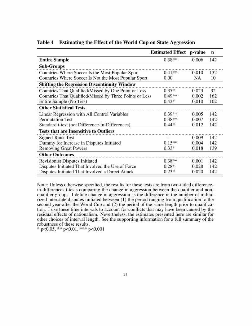
Table 4 Estimating the Effect of the World Cup on State Aggression

Estimated Effect p-value nEntire Sample 0.38** 0.006 142Sub-GroupsCountries Where Soccer Is the Most Popular Sport 0.41** 0.010 132Countries Where Soccer Is Not the Most Popular Sport 0.00** NA 10Shifting the Regression Discontinuity WindowCountries That Qualified/Missed by One Point or Less 0.37** 0.023 92Countries That Qualified/Missed by Three Points or Less 0.49** 0.002 162Entire Sample (No Ties) 0.43** 0.010 102Other Statistical TestsLinear Regression with All Control Variables 0.39** 0.005 142Permutation Test 0.38** 0.007 142Standard t-test (not Difference-in-Differences) 0.44** 0.012 142Tests that are Insensitive to OutliersSigned-Rank Test –** 0.009 142Dummy for Increase in Disputes Initiated 0.15** 0.004 142Removing Great Powers 0.33** 0.018 139Other OutcomesRevisionist Disputes Initiated 0.38** 0.001 142Disputes Initiated That Involved the Use of Force 0.28** 0.028 142Disputes Initiated That Involved a Direct Attack 0.23** 0.020 142

Note: Unless otherwise specified, the results for these tests are from two-tailed difference-in-differences t-tests comparing the change in aggression between the qualifier and non-qualifier groups. I define change in aggression as the difference in the number of milita-rized interstate disputes initiated between (1) the period ranging from qualification to thesecond year after the World Cup and (2) the period of the same length prior to qualifica-tion. I use these time intervals to account for conflicts that may have been caused by theresidual effects of nationalism. Nevertheless, the estimates presented here are similar forother choices of interval length. See the supporting information for a full summary of therobustness of these results.* p<0.05, ** p<0.01, *** p<0.001

21

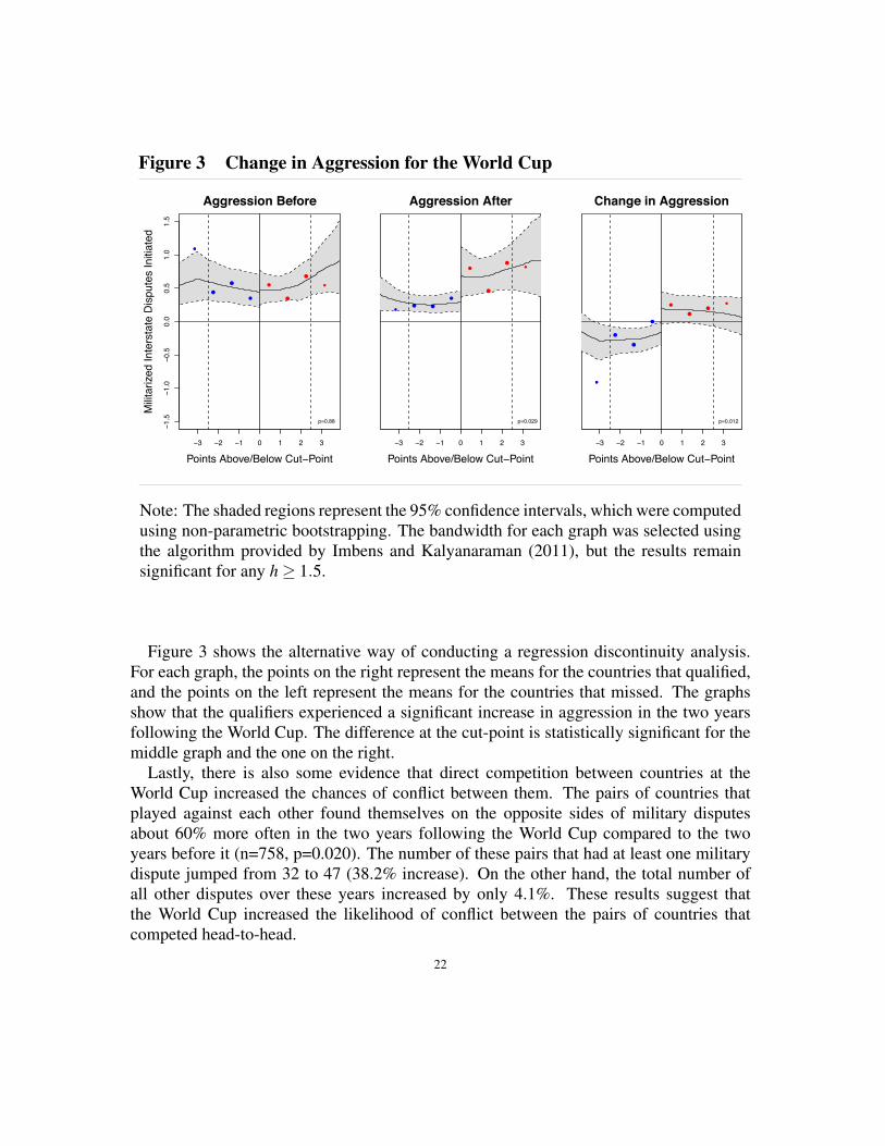
Figure 3 Change in Aggression for the World Cup

●

●

●

●

●

●

●

−1.5

−1.0

−0.5

0.0

0.5

1.0

1.5

Aggression Before

Points Above/Below Cut−Point

Milit

arize

d In

ters

tate

Dis

pute

s In

itiat

ed

●

●

●

●

●

● ● ●

●

●

●

●

●

●

●

●

●

●

●

●

● ● ●

−3 −2 −1 0 1 2 3

p=0.88

●

●

●

●

●● ●

●

Aggression After

Points Above/Below Cut−Point

●

●

●●

●

●

●

●●

●

●

●

●● ●

●

●

●

●●

●

●

●

●

−3 −2 −1 0 1 2 3

p=0.029

●

●

●

●

●

●

●

●

Change in Aggression

Points Above/Below Cut−Point

●

●●

●

●

●

●

●

●

●

●

●

●

●

●●

●

●

−3 −2 −1 0 1 2 3

p=0.012

Note: The shaded regions represent the 95% confidence intervals, which were computedusing non-parametric bootstrapping. The bandwidth for each graph was selected usingthe algorithm provided by Imbens and Kalyanaraman (2011), but the results remainsignificant for any h � 1.5.

Figure 3 shows the alternative way of conducting a regression discontinuity analysis.For each graph, the points on the right represent the means for the countries that qualified,and the points on the left represent the means for the countries that missed. The graphsshow that the qualifiers experienced a significant increase in aggression in the two yearsfollowing the World Cup. The difference at the cut-point is statistically significant for themiddle graph and the one on the right.

Lastly, there is also some evidence that direct competition between countries at theWorld Cup increased the chances of conflict between them. The pairs of countries thatplayed against each other found themselves on the opposite sides of military disputesabout 60% more often in the two years following the World Cup compared to the twoyears before it (n=758, p=0.020). The number of these pairs that had at least one militarydispute jumped from 32 to 47 (38.2% increase). On the other hand, the total number ofall other disputes over these years increased by only 4.1%. These results suggest thatthe World Cup increased the likelihood of conflict between the pairs of countries thatcompeted head-to-head.

22

Figure 4 Conflict Between Countries That Played at the World Cup

Total Militarized Interstate Dipsutes

Pairs with at Least One Dispute

59

47

34

37

30

40

50

60

Two Years Before Two Years AfterTime Period

SECTION 6: EVIDENCE OF THE MECHANISM

As I discussed earlier, past historical evidence suggests that international sports leadto conflict because they incite mass nationalism. By doing so, they give leaders moreincentive and opportunity to initiate military conflicts. Given the large estimated effect ofthe World Cup on state aggression found in the previous section, it is worth asking if thereis also evidence that this mechanism is at work.

In fact, there are two noteworthy trends in the aggregate data that suggests that the WorldCup led to more nationalism and militarism. Along with increasing state aggression, theWorld Cup also appears to have encouraged military participation and military spending.For military participation, the estimated effect is quite large. About 46% of the qualifiersexperienced an increase in military personnel following the World Cup, whereas only30% of the non-qualifiers did (p=0.047). Similarly, the countries that barely qualifiedexperienced a much larger increase in military spending than the countries that barelymissed (p=0.071). These results provide further evidence that the World Cup had an effecton mass nationalism as well as government decision-making.

There are also cases from the sample that suggest that World Cup nationalism is behindthe results. The first is Senegal (2002), which initiated a dispute against Gambia abouttwo weeks after its final World Cup game. In fact, the only time that Senegal has evergone to the World Cup was in 2002, and the dispute that it started just afterward was the

23

only dispute that it was involved in from 1993-2010. This case is also striking becauseSenegal did surprisingly well at the World Cup. In the group stage, it defeated France, thedefending World Cup champion and its former colonizer. The victory was so remarkablethat CNN lists it as one of the ten greatest upsets in World Cup history. Senegal then beatSweden in the first round of the knockout stage, making it just the second African team toadvance to the quarterfinals. It lost its next game to Turkey 0-1, exiting the tournament onJune 22, 2002.

No doubt, the World Cup created a powerful surge of nationalism in Senegal, whichbegan immediately after qualification. Senegal’s president, Abdoulaye Wade, was visit-ing Jacques Chirac in France at the time, but returned home early to celebrate Senegal’squalification for the World Cup. As he explained, “it’s the most important thing that canhappen to any country and I will join the team and the nation in celebrating by reducingthe amount of time I was expected to stay in Paris” (Ralph 2007). To reward his players,he invited them to his palace and presented each of them with bonuses of about $15,000.Nation-wide celebrations also broke out after Senegal defeated France and Sweden, andthey were encouraged by the government. For instance, after the win over France, Presi-dent Wade declared a national holiday and paraded around the capital in a vehicle with thetop open so that fans could see him juggling a soccer ball.

On July 7, 2002, just 15 days after losing to Turkey in the knockout stage, Senegalinitiated a military dispute against Gambia. Specifically, it asserted its control over theCasamance region in southern Senegal by expelling a group of rebels who were allegedlysupported by Gambia. Senegal then deployed troops along the Gambian border to ensurethat the rebels would not reenter the country. This example featured clear military action,but it is most notable because of its timing. The fact that it is the only dispute that Senegalinitiated in an almost twenty-year period and that it happened just after Senegal madeits only World Cup appearance in history suggests that sports nationalism can encourageleaders to make aggressive foreign policy moves.

A second notable case from the sample is Cameroon (1994), which illustrates how theWorld Cup can lead to reoccurring disputes. In October of 1993, Cameroon qualified forthe World Cup, causing celebrations to erupt throughout the country. In the followingMarch, about three months before the World Cup was set to begin, Cameroon invadedthe Bakassi Peninsula, an oil-rich region located between Cameroon and Nigeria. Thisdispute was the first that Cameroon was involved in since 1987. It resulted in a seriesof clashes between Cameroon and Nigerian troops in the following years, two of whichwere coded as new disputes initiated by Cameroon (December 1995 and March 1996).This case demonstrates how one dispute can lead to a series of conflicts, which may helpexplain the longevity of the effect.

These cases also suggest another possible mechanism that may be at work. In somecases, leaders may not just be reacting to changing public opinion; they may be passionatefans themselves who become more nationalistic from watching their teams play. No doubt,

24

it is common for government leaders to attend games, and some even schedule their cabinetmeetings around them so that they can watch their teams play on television (Markovits andRensmann 2010). After all, most state leaders are men, who are much more likely to besports fans than women. Simply watching games could therefore encourage some leadersto see other states as competitors, which would bypass the public opinion mechanism.

Of course, it is very difficult to assess this mechanism empirically, since it requiresknowing leaders’ inner thoughts. For instance, Senegal’s president seemed passionateabout soccer, but it all might have been for show. There are also clear examples of leaderslike Hitler who did not care about sports for their own sake, and who were just interestedin how they could be used to manipulate public opinion. Thus, this mechanism cannotexplain all of the conflicts that have occurred because of sports nationalism, but it mayexplain some of them, and it is therefore worth taking seriously.

CONCLUSIONThis study provides strong evidence that surges of nationalism can have a substantial

impact on interstate conflict. In doing so, it confirms an important causal relationship thathas been assumed in much international relations scholarship, but had yet to be empiricallyestablished. Put simply, the history of international sports provides enough qualitative andquantitative evidence to conclude that fluctuations in nationalism can have a large impacton state aggression.

In short, nationalism should continue to play an important role in the study of inter-national relations. The premise that nationalism causes conflict can be very useful forinterpreting history, constructing theories, and making arguments to policymakers. Morework is also needed to identify other potentially dangerous sources of nationalism. Onepromising avenue would be to look at whether major national achievements and tragediestend to increase state aggression in the short run. Some research has already been done onhow nationalism from September 11 made many Americans more willing to invade Iraq(McCartney 2004), but there is still room for a broader theory that takes into account otherevents that cause temporary spikes in nationalism.

This study also has some important policy implications. Since international sports area powerful source of nationalism, we should try to limit the ability of certain leaders touse that nationalism to increase domestic support for their aggressive foreign policies. Forexample, allowing Putin to host the 2014 Winter Olympics and 2018 World Cup was apoor decision, and international sports organizations should be careful not to make similarmistakes in the future.

We might also consider having some sporting events where countries play as smallregional blocks like a Scandinavian team and Balkans team. This format would encouragepeople to identify with their regions rather than their nations, and could therefore improvehow people perceive neighboring states. They would be allies rather than competitors.Moreover, this format would ensure that a country’s opponents would typically be groups

25

of countries that were further away geographically and less likely to be possible targets offuture military aggression. Thus, this format would probably have a much more positiveeffect on international relations than the current practice of constantly pitting countriesagainst each other on the international stage.

26

REFERENCES

Anderson, Benedict. 1991. Imagined Communities: Reflections on the Origin and Spreadof Nationalism. Rev. ed. New York: Verso.

Anderson, Thomas. 1983. The War of the Dispossessed: Honduras and El Salvador.Lincoln: University of Nebraska Press.

Belmary, Ramadan. 2009. “Egypt & Algeria Soccer Spat Reaches Arab League.” AlArabiya News, 23 November.

Byman, Daniel and Kenneth Pollack. 2001. “Let Us Now Praise Great Men: Bringing theStatesman Back In.” International Security 25(4): 107-146.

Cattaneo, Matias, Brigham Frandsen, and Rocio Titiunik. 2015. “Randomization Infer-ence in the Regression Discontinuity Design: An Application to Party Advantages inthe US Senate.” Journal of Causal Inference 3(1): 1-24.

Cederman, Lars-Erik, T. Camber Warren and Didier Sornette. 2011. “Testing Clausewitz:Nationalism, Mass Mobilization, and the Severity of War.” International Organization65(4), 605-38.

Cha, Victor. 2009. “A Theory of Sport and Politics.” The International Journal of theHistory of Sport 26(11), 1581-1610

Colgan, Jeff. 2010. “Oil and Revolutionary Governments: Fuel for International Conflict.”International Organization 64(4): 661-694.

Ðordevic, Ivan. 2012. “Twenty Years Later: The War Did (not) Begin at Maksimir. AnAnthropological Analysis of the Media Narratives About a Never Ended Football Game.”Bulletin of the Ethnographic Institute SASA, 201-215

Dunning, Thad. 2012. Natural Experiments in the Social Sciences: A Design-BasedApproach. New York: Cambridge University Press.

Frith, David. 2013. Bodyline Autopsy: The Full Story of the Most Sensational Test CricketSeries: Australia v England 1932-33. Aurum Press Limited.

Garland, Jon, and Mike Rowe. 1999. “War Minus the Shooting?: Jingoism, the EnglishPress, and Euro 96.” Journal of Sport and Social Issues 23(1), 80-95.

Goldblatt, David. 2008. The Ball Is Round: A Global History of Soccer. New York:Penguin.

Ghosn, Faten, Glenn Palmer, and Stuart Bremer. 2004. “The MID3 Data Set, 1993-2001:Procedures, Coding Rules, and Description.” Conflict Management and Peace Science21(2), 133-54.

Hassin, Ran, et al. 2007. “Subliminal Exposure to National Flags Affects PoliticalThought and Behavior.” Proceedings of the National Academy of Sciences 104(50):19757-19761.

Hitchens, Christopher. 2010. “Why the Olympics and Other Sports Cause Conflict.”Newsweek.

27

Hobsbawm, Eric. 1990. Nations and Nationalism since 1780: Programme, Myth, Reality.New York: Cambridge University Press.

Imbens, Guido, and Karthik Kalyanaraman. 2011. “Optimal Bandwidth Choice for theRegression Discontinuity Estimator.” The Review of Economic Studies: rdr043.

Kapuscinski, Ryszard. 2013. The Soccer War. New York: Random House LLC.Kemmelmeier, Markus, and David Winter. 2008. “Sowing Patriotism, but Reaping Na-

tionalism? Consequences of Exposure to the American Flag.” Political Psychology29(6): 859-879.

Keohane, Robert, and Joseph Nye Jr. 2001. “Between Centralization and Fragmentation:The Club Model of Multilateral Cooperation and Problems of Democratic Legitimacy.”

Kowalski, Ronald, and Dilwyn Porter. 1997. “Political football: Moscow Dynamo inBritain, 1945.” The International Journal of the History of Sport 14(2): 100-121.

Krüger, Arnd. 1998. “The Role of Sport in German Politics, 1918-1945.” In Sport andInternational Politics: Impact of Fascism and Communism on Sport, edited by PierreArnaud and Jim Riordan, 79-93. New York: Routledge.

Lai, Brian, and Dan Slater. 2006. “Institutions of the Offensive: Domestic Sources of Dis-pute Initiation in Authoritarian Regimes, 1950Ð1992.” American Journal of PoliticalScience 50(1): 113-126.

Large, David. 2007. Nazi Games: The Olympics of 1936. New York: WW Norton &Company.

Lee, David. 2008. “Randomized Experiments from Non-Random Selection in US HouseElections.” Journal of Econometrics 142(2), 675-697.

Lee, David, and David Card. 2008. “Regression Discontinuity Inference with Specifica-tion Error.” Journal of Econometrics 142(2): 655-674.

Lindsey, Ursula. 2009. “The Soccer Wars.” Foreign Policy.Mansfield, Edward, and Jack Snyder. 1995. “Democratization and the Danger of War.”

International Security, 5-38.Markovits, Andrei, and Lars Rensmann. 2010. Gaming the World: How Sports are Re-

shaping Global Politics and Culture. Princeton, NJ: Princeton University Press.Martin, Simon. 2004. Football and Fascism: The National Game Under Mussolini. New

York: BergMcCartney, Paul. 2002. “American Nationalism and U.S. Foreign Policy from September

11 to the Iraq War.” Political Science Quarterly 119(3): 399-423.Mearsheimer, John. 1990. “Why We Will Soon Miss the Cold War.” The Atlantic Monthly

266(2), 35-50.Mehler, Andreas. 2008. “Political Discourse in Football Coverage: The Cases of Côte

d’Ivoire and Ghana.” Soccer & Society 9(1): 96-110.Orwell, George. 1945. “The Sporting Spirit.” The London Tribune.Pape, Robert. 1996. Bombing to Win: Air Power and Coercion in War. New York: Cornell

University Press.

28

Posen, Barry. 1993. “The Security Dilemma and Ethnic Conflict.” Survival 35(1), 27-47.Posen, Barry R. 2013. “Pull Back: The Case for a Less Activist Foreign Policy.” Foreign

Affairs 92(1): 116-28.Ralph, Michael. 2007. “ ‘Crimes of History’ Senegalese Soccer and the Forensics of

Slavery.” Souls 9(3): 193-222.Reid, Gerard. 2000. Football and War. Cheshire: Sigma Leisure.Riach, James. 2014. “Albanian FA Claims Serbian Police Attacked Players After Aban-

doned Match.” The Guardian, October 16.Rippon, Anton. 2006. Hitler’s Olympics: The Story of the 1936 Nazi Games. South

Yorkshire: Pen & Sword Books.Rosato, Sebastian. 2011. Europe United. Ithaca, New York: Cornell University Press.Rosato, Sebastian. 2003. “The Flawed Logic of Democratic Peace Theory.” American

Political Science Review 97 (4): 585-602.Robinson, Amanda L. “National Versus Ethnic Identification in Africa: Modernization,

Colonial Legacy, and the Origins of Territorial Nationalism.” World Politics 66(4):709-746.

Sack, Allen, and Zeljan Suster. 2000. “Soccer and Croatian Nationalism a Prelude toWar.” Journal of Sport and Social Issues 24(3), 305-20.

Schama, Simon. 2014. Interview on Bill Maher (21 March).Schrock-Jacobson, Gretchen. 2012. “The Violent Consequences of the Nation: National-

ism and the Initiation of Interstate War.” Journal of Conflict Resolution 56(5), 825-52.Shenker, Jack. 2009. “More to Egypt Riots than Football.” The Guardian, November 25.Snyder, Jack. From Voting to Violence: Democratization and Nationalist Conflict. New

York: Norton, 2000.Steenveld, Lynette, and Larry Strelitz. 1998. “The 1995 Rugby World Cup and the Politics

of Nation-Building in South Africa.” Media, Culture and Society 20(4), 609-29.Stephens, Scott. 2007. “Iraq’s Asia Cup Victory Hides Reality of Ungovernable Society.”

Eureka Street 17(15), 22.Swan, Wayne. 2013. “Bodyline’s Final Legacy May Be an Australian Republic” The

Sydney Morning Herald. 25 January.Van Evera, Stephen. 1994. “Hypotheses on Nationalism and War.” International Security

18(4), 5-39.Vincent, John, et al. 2010. “England Expects: English Newspapers’ Narratives About the

English Football Team in the 2006 World Cup.” International Review for the Sociologyof Sport 45(2), 199-223.

Voeten, Erik. 2013. “Does Participation in International Organizations Increase Coopera-tion?” The Review of International Organizations 8(3), 1-24.

Walt, Stephen. 2011. “Nationalism Rules.” Foreign Policy.Wendt, Alexander. 1999. Social Theory of International Politics. New York: Cambridge

University Press.

29

United We Fight: DemocraticUnity and State Aggression

Andrew Bertoli

ABSTRACT. Are democratic leaders more likely to use force abroad when their co-partisanscontrol the main bodies of government? Past studies have sought to answer this questionwith regression analysis, but their statistical models lead to incompatible results. I shednew light on this debate using a regression discontinuity design. Looking at democraciesfrom 1815-2010, I compare cases where political parties barely gained control of govern-ment to cases where they barely fell short of doing so. The results provide compellingevidence that government unity increases state aggression. Specifically, I find that unitedgovernment makes countries much more likely to initiate high-level disputes. The effectis particularly notable for the United States. These results underscore the importance ofbeing alert to the impact of domestic political developments on foreign policy.

In August of 2013, Republican leaders in the House of Representatives announcedthat Obama’s request to use force against Syria would not pass. Obama had asked theRepublican-controlled House for authorization to retaliate against Assad for his use ofchemical weapons in the Syrian Civil War. While it is not necessary for presidents to re-ceive permission from the House for conflicts lasting shorter than 60 days, it would havelegitimized Obama’s decision, ensured that Republicans would not try to punish him foracting without their approval, and allowed him to stay involved in the conflict if it lastedlonger than two months. However, the normally hawkish Republicans refused to authorizethe military strike. As Republican Representative Tim Griffin explained, “I am reluctantto give him a license for war when, with all due respect, I have little confidence he knowswhat he is doing.”1 Clearly, circumstances were very different from the situation in 2009and 2010, when the legislative branch was controlled by the Democrats. During this pe-riod, Obama had a substantial amount of freedom when it came to foreign policy, allowinghim to shift military troops from Iraq to Afghanistan and expand the drone program with-out having to worry about congressional resistance.

This case raises a key question about the impact of domestic factors on foreign policy:Are democracies more likely to take military action when their governments are united,

I would like to thank Jasjeet Sekhon, Ron Hassner, Thad Dunning, Aila Matanock, Michaela Mattes,Fredrick Salve, Josh Kalla, Caroline Brandt, Nina Kelsey, Jason Klocek, Anne Meng, Tara Buss, AliceCiciora, Elizabeth Herman, Melissa Carlson, Bora Park, and Jay Varellas for helpful comments.1The New York Times, 31 August 2013.

30

meaning that their executive and legislative branches are both controlled by a single party?No doubt, there are compelling reasons to think that united government may make coun-tries more aggressive. On one hand, leaders of united governments may be less constrainedwhen it comes to foreign policy, making it easier to take military action against other states(Howell and Pevehouse 2005). Additionally, they may feel that they are less likely tobe punished by the legislature for taking unpopular military action. However, there arealso reasons to think that united government might not make aggression more likely. Na-tional security information is often kept secret, so decisions by leaders to use force maybe largely uninfluenced by the legislature (Rosato 2003). Leaders facing strong oppositionparties might also be unable to advance their agendas at home, giving them more reasonto focus on international relations where they may have more autonomy (Brulé 2006).

This question has important implications for our understanding of international rela-tions. First, one proposed explanation for the democratic peace is that strong opposi-tion parties make it difficult for leaders to take military action against other countries. Ifdemocracies tend to behave more aggressively when they are united, then it would provideevidence for this important causal mechanism while also pointing to a caveat of the theory:that the democratic peace is more likely to hold when democracies are divided. Second, ifgovernment unity increases state aggression, then policymakers and the public should bealert to the potential danger of unnecessary conflicts when one party is in power.

But despite the importance of this question, past researchers have been unable to reacha consensus on how united government affects state aggression. Their studies, which relyprimarily on regression analysis, come to a wide range of competing conclusions. Manyfind that united government increases state aggression (Clark 2000; Clark and Nordstrom2006; Brulé 2006; Pevehouse 2005). However, others find little evidence that this is thecase, instead concluding that politics stop at the water’s edge (Gowa 1998; Schultz 1999;Leblang and Chan 2003). Put simply, efforts to resolve this question with statistical modelshave led to incompatible results.

I shed new light on this debate by taking advantage of a natural experiment where gov-ernment unity was assigned to countries as-if randomly. Specifically, I compare caseswhere political parties barely gained control of their governments to cases where theybarely fell short of doing so. The idea is that when parties are on the verge of achievingunited government, it is basically a coin-flip which ones barely succeed and which onesbarely fail. This conjecture is likely true because large national elections have many un-predictable elements. Thus, it would be very difficult for parties to know exactly how closethey were to united government beforehand and precisely manipulate turnout to get justenough votes to take control of government. In short, when countries are at the threshold,whether they become united or divided is largely left up to chance.

The results provide compelling evidence that united government increases state aggres-sion. While the countries with barely united and barely divided governments were verysimilar prior to the elections, the countries with barely united governments became much

31

more aggressive after their governments came to power. Specifically, they were much morelikely to initiate high-level military disputes against other states. However, they were notsignificantly more likely to initiate low-level disputes.

This paper proceeds as follows. Section 1 considers several theoretical arguments aboutthe relationship between united government and state aggression. Section 2 reviews theobservational evidence. Section 3 lays out the research design in more detail and verifiesthat the countries with barely united and barely divided governments were very similar onpre-treatment characteristics. Section 4 analyzes the results with a number of statisticalmethods. Section 5 considers the broader implications of these findings. The final sectionconcludes.

SECTION 1: THEORYThe argument that united government increases state aggression rests on three basic

ideas. The first is that opposition parties will constrain leaders when government is di-vided, specifically because they have the opportunity and incentive to do so. The secondis that leaders will not become less interested in foreign policy during times of unitedgovernment, say because they will be much more focused on passing domestic legislationthrough a favorable legislature. The third is that the countries that are the potential targetsof aggression will not be more willing to make concessions when facing a united gov-ernment, because they realize that they are negotiating with a less constrained adversary.Assuming that these conditions hold, united government should tend to increase the like-lihood of state aggression. However, if even one of these conditions is typically untrue,then the effect of united government could be negligible.

Opposition Parties. Let us start with the question of whether opposition parties can betterconstrain leaders when government is divided. The most obvious way that they could doso is by refusing to give leaders permission to use military force abroad (Brulé 2006).For instance, if the legislature is responsible for approving any military engagement, thenopposition parties in divided governments may simply be able to vote down such policieswhen leaders request them. Thus, the legislature could act as a veto player that simplydenies the leader permission to use force (Tsebelis 1995).

However, it is typically not this easy for opposition parties to constrain leaders. Al-though most democratic legislatures are formally responsible for authorizing military ac-tion, leaders often launch military strikes without legislative approval. For instance, theUnited States government used force against other countries in 126 separate military dis-putes from 1815-2010, but only 13 of these cases were actually authorized by Congress,and only four involved a formal declaration of war (French and Bradshaw 2014). This abil-ity of leaders to bypass the legislature is partly explained by the need to make decisionsquickly in international crises and keep vital national security information secret (Rosato

32

2003). Thus, the formal institutional power that legislatures are usually granted over thedecision to use force often fails to keep executives in check.

A more likely way that the opposition can exert influence in divided government isby threatening to punish leaders. Strong opposition parties can often defund unwantedmilitary campaigns, remove leaders from office, or refuse to cooperate in other policyareas. Thus, leaders who face a divided government might realize that acting against thewishes of the opposition would be costly and opt not to use military force. This typeof deterrence would primarily apply to cases that involve the actual use of force againstother states. After all, the legislature would not be able to defund or credibly punish verylow-level disputes that merely involve saber-rattling. Thus, we should expect that a strongopposition party could, at most, prevent leaders from taking significant military actionagainst other countries.

Of course, even if opposition parties have the power to constrain aggression, they mustalso have incentives to do so. Whether they do will largely depend on how much theirforeign policy goals differ from those of the leader. For instance, if one party had muchmore dovish foreign policy preferences than the other, then we might expect military con-flict to occur more when the hawkish party achieves a united government. Another caseof competing foreign policies could arise if both parties were equally willing to use forcebut had very different interests. They might favor different allies or fear different foreignenemies, and thus block each other’s military initiatives whenever possible.

However, even if the leader and the opposition agree on when force should be used,opposition parties might have other reasons to prevent leaders from taking military action.For example, they might doubt that the leader is competent enough to manage the conflicteffectively, as Representative Tim Griffin claimed when Obama requested authorizationto attack Syria. Another possibility is that the opposition might fear that foreign conflictwould improve the leader’s approval rating. A number of scholars have shown that inter-state conflict often produces a “Rally ’Round the Flag Effect” that increases the executive’spopularity (Mueller 1970; Oneal and Bryan 1995). By doing so, it may strengthen theleader’s party at the expense of the opposition, since popular executives can improve theelectoral prospects of their co-partisans in the legislature (Campbell and Sumners 1990;Howell and Pevehouse 2005). Thus, even when the members of the opposition largelyshare the leaders’ foreign policy goals, they may still fear that military conflict will ulti-mately hurt them in the polls.

Leaders. A second condition that must hold is that united government cannot distractleaders from foreign policy. If it encourages them to turn their attention to domestic poli-tics, where they will have an easier time passing legislation, then united government mightmake countries less aggressive.

However, this logic assumes that leaders often struggle to focus on multiple things atonce, even when the conditions make advancing their agenda relatively easy. Given that

33

they have the manpower and resources to research many issues simultaneously, it is un-likely that greater opportunity domestically would divert attention away from foreign pol-icy. In fact, leaders might not need to spend as much time on domestic policy whengovernment is united, because they will not have to negotiate with the other party on everypiece of legislation. Thus, there is little reason to think that united government will causeleaders to pay less attention to foreign policy.

Target States. Lastly, because military conflict often results from one country refusing togive into another country’s demands, it is also important to consider how united govern-ment might influence the strategy of a democracy’s adversaries. If these states recognizethat they are negotiating with a less constrained leader, they might be more willing to makeconcessions that prevent conflict from breaking out.

However, there are several reasons for believing that target states would not be moreconciliatory when facing a united government. First, the target country might not realizethat the democratic leader is in a better position to use force against it. Given that politicalscientists disagree about whether united government gives leaders more freedom in foreignpolicy, it is likely that many target countries are also unsure whether they are negotiatingwith a less constrained state. Second, even if the leaders in the target country understoodthe increased possibility of being attack, they might still prefer to risk conflict than makeconcessions. For instance, they might fear how looking weak on the international stagewould hurt them in domestic politics, or they might be very confident in their chances ofwinning a fight. Third, the target country might doubt the resolve of the united democracyif the opposition parties in that democracy, unable to prevent the conflict through legislativeaction, voice their opposition to the conflict in the media. Thus, there is good reason tothink that target states will not necessarily be more willing to make concessions whenfacing a united government.

SECTION 2: EXISTING EVIDENCEExisting evidence about the relationship between united government and state aggres-

sion is unclear. On one hand, the U.S. record of major war suggests that government unityhas a large impact on a country’s likelihood of engaging in large-scale military conflict.Since the Revolutionary War, there have been nine interstate wars that involved at least1,000 U.S. battle deaths. The American government was united before entering all butone of them�the recent war in Afghanistan following September 11. As Figure 1 shows,this number is strikingly large given that the United States has only been united for abouthalf of its history. In fact, the wars started under united government resulted in a total of434,609 American battle deaths, while the war started under divided government resultedin 1,724 American battle deaths.

34

Figure 1. Interstate Wars with at Least 1,000 U.S. Battle Deaths

● ● ● ● ● ● ●

●

●

Divided

United

1800 1850 1900 1950 2000

However, this correlation between united government and international conflict mightbe explained by confounding factors rather than a true causal relationship. For example,publics might be more willing to elect a united government when the international systemseems particularly dangerous. To overcome this problem, a number of studies have usedregression analysis to control for possible confounders. However, these studies come tocompeting conclusions. For example, Clark and Nordstrom (2006) find that united govern-ment increases the likelihood that countries will initiate military disputes, while Schultz(1999) finds little statistical evidence that opposition parties effectively constrain leadersfrom initiating military disputes. Leblang and Chan (2003) reach similar conclusions wheninvestigating involvement in interstate wars.

Even research that just focuses on the United States has failed to reach agreement. Gowa(1998) finds that united government has a negative and insignificant effect on U.S. mili-tary disputes. On the other hand, Clark (2000) and Brulé (2006) conclude that governmentunity increases the likelihood that the United States will initiate military disputes. Mean-while, Howell and Pevehouse (2005) find that the United States tends to initiate morehigh-level disputes under united government, but that this pattern does not hold for low-level disputes. Put simply, regression analysis has failed to produce a clear answer, whichis not entirely surprising given that regression results can vary widely based on modelspecification and the variables that researchers choose to control.

The ideal way to get around this problem would be to run an experiment where we tooka large group of countries and randomly assigned some to be united and others to be di-vided. Randomization would get around the confounding problem because it would createbalance across observable and unobservable characteristics. Thus, it would allow for usto make a fair comparison between countries with united and divided governments. If thegroup of countries with united governments behaved much more aggressively, we couldconclude that this difference was due to government unity rather than some confoundingfactor.

Of course, we cannot run a real experiment to answer this question, because assigninga large number of countries to be united or divided is infeasible. However, the process

35

of national elections within democracies created a natural experiment that is very similarto the ideal study described above. I turn my attention to this natural experiment in thefollowing sections.

SECTION 3: RESEARCH DESIGNStrategy for Identifying the Causal Effect. This paper tests how united governmentaffects state aggression by using a regression discontinuity (RD) design. RD is a quasi-experimental approach that can be used when a treatment is given to units that surpassan important cut-point in a scoring system (Dunning 2012). The idea is to compare thegroup of units that scored just above the cut-point to the group that scored just below it.As long as there is some randomness in the scoring process, it should be close to randomwhich units end up on either side of the cut-point (Lee 2008). Thus, the units just abovethe cut-point should be, on average, similar to the units just below the cut-point, exceptthat the units above received the treatment and the units below did not.

In political science, RD is most often used to estimate the effects of winning close elec-tions on a variety of outcomes, including personal wealth and the probability that a personor party will win the next election (Eggers and Hainmueller 2009; Titiunik 2009; Broock-man 2009; Gerber, Kessler, and Meredith 2011; Eggers, Folke, Fowler, Hainmueller, Hall,and Snyder 2013). However, RD has also been used to study questions in internationalrelations, like how being elected to the UN Security Council affects the willingness ofcountries to contribute to peacekeeping missions (Voeten 2013), how barely qualifying forthe World Cup affects state aggression (Bertoli 2016), and how electing a younger leaderaffects a country’s likelihood of engaging in military conflict (Bertoli, Dafoe, and Trager2016).

For this study, I compare cases where parties barely gained control of government tocases where they barely fell short of doing so. For instance, in 1990, the strongest party inCosta Rica, the Social Christian Unity Party, won the presidency by about 4% of the voteand gained control of the parliament by exactly one seat. However, when the next elec-tion came around in 1994, the situation was reversed. The strongest party (this time theNational Liberation Party) won the presidency by 2% of the vote but fell short of gainingcontrol of the parliament by exactly one seat. In very close national elections like these,whether countries ended up barely united or barely divided should be essentially random.Thus, the group of countries that where barely united should be, on average, pretty sim-ilar to the group of countries that were barely divided, except for the key difference ingovernment unity.

Democracy and Election Data Sources. To construct the dataset, I began by identify-ing every democracy in the international system from 1815-2010. Following past stud-ies (Schrock-Jacobson 2012; Marshall, Gurr, and Jaggers 2013), I counted a country as

36

a democracy in a given year if it had a POLITY IV Institutionalized Democracy Scoreabove five. After creating the list of democracies, I collected election data from an numberof sources. The key volumes were Elections in the Americas: A Data Handbook (2005),Elections in Europe: A Data Handbook (2010), Elections in Africa: A Data Handbook(1999), and Elections in Asia and the Pacific: A Data Handbook (2001). I also had touse some online databases to get information on elections in recent years. These sourcesincluded the International Foundation for Electoral Systems’ Election Guide, the AfricanElection Database, and the European Election Database.

Scenarios. There are three basic ways that power is shared between different governmentbodies in a democracy. First, some countries have an independently elected executivebranch and exactly one legislative body (unicameral presidential systems). These coun-tries are united if one party controls the executive and legislative body, and they are dividedotherwise. Countries with this form of government include Austria, France, Finland, Ire-land, and South Korea. Second, some democracies have two legislative bodies, such as ahouse and senate, while lacking an independently elected executive branch (bicameral par-liamentary systems). In these countries, the executive is typically elected by one of the twolegislative bodies. Countries with this government structure include Australia, Belgium,Italy, Japan, and Spain. These countries are united if one party controls both legislativebodies. Third, some countries have an independently elected executive branch and twolegislative bodies (bicameral presidential systems), like the United States, Brazil, Mexico,Colombia, and the Philippines. In order for these countries to be united, a party must con-trol all three of these government organizations. I exclude from this analysis democraciesthat have only one legislative branch that chooses a prime minister (unicameral parliamen-tary systems), since these countries are always united under whatever party or coalitioncontrols the legislature.

It is fairly straightforward to think about how close governments are to being unitedin the three main contexts described above. Figure 2 illustrates government control forcountries with a president and one legislative body as a two-dimensional RD. Each pointrepresents the level of control for the strongest party in the country. Points to the rightof the vertical axis are cases where the party controlled the legislature, and points abovethe horizontal axis are cases where the party controlled the presidency. Thus, the up-per right-hand quadrant contains the cases where the most powerful party controlled boththe executive and legislative bodies (united government), and all other quadrants containdivided governments. Countries that were barely united or barely divided are the onesthat are very close to being inside or outside of the upper right-hand quadrant. Similarly,Figure 3 depicts countries with two legislative bodies and no independently elected pres-ident. Again, points in the upper right hand quadrant represent united government, whilepoints in all other quadrants depict divided governments. Countries with an independentlyelected executive and two legislative bodies must be thought of as a three-dimensional

37

Figure 2. Strength of Most Powerful Party in Elections witha President and Legislature

●

●

●

●

●●

●

●

●

●

●

● ●●●

●

●

● ●

●

●

●

●

●

●

●

●

●

●

●

●

●

●

●

●

●

●

●

●

●

●

●

●

●

●●

●

●

●

●

●

●

●

● ● ●●

●

●

●

●

●●

●

●

●

●

●

●

●

●

●●

●

●

●

●

●

●● ●

●●

●

●

●

●

●

●

●●

● ●

●

●●

●

●

●

●

●

●

●●

●

●

●

●

●

●

0.0

0.4

0.8

−0.2 0.0 0.2 0.4Percent of Seats from Controlling Legislature

Perc

ent o

f Vot

es fr

om C

ontro

lling

Pres

iden

cy

Figure 3. Strength of Most Powerful Party in Elections withTwo Legislative Bodies

●●

●

●● ●●

● ●

●●

● ●●

●●

●●

●

●

●

●

●

●

●

●

●

●

●

●

● ●

●

●●

●

●

●

●

●●

●

●

●

●

●

●

●

●●●

●

●

●

●

●

● ●

●●

●

●

●

●●● ●

●

●

●●

●

●

● ●

●

●●

●

●

● ●

●

●●

●●●●●

●●

●●

●

●

●●

●●

●

●

●

●

●●

●●●

●●

−0.25

0.00

0.25

0.50

−0.2 0.0 0.2Percent of Seats from Controlling House

Perc

ent o

f Sea

ts fr

om C

ontro

lling

Sena

te

38

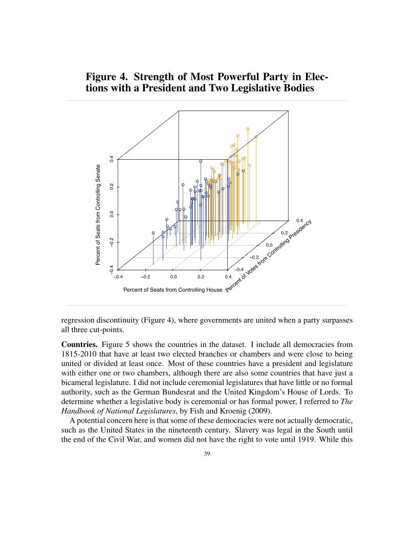
Figure 4. Strength of Most Powerful Party in Elec-tions with a President and Two Legislative Bodies

−0.4 −0.2 0.0 0.2 0.4

−0.4

−0.2

0.0

0.2

0.4

−0.4

−0.2

0.0

0.2

0.4

Percent of Seats from Controlling House

Perc

ent o

f Sea

ts fr

om C

ontro

lling

Sena

te

●

●

●

●

●

●●

●

●

●

●

●

●

●

●

●

●

●

●

●

●

●

●

●

●

●

●

●

●●

●

●●

●

●

●

●

●●

●

●● ●

●

●

●

●

●●

●

●

●

●

●

●

●

●

●

●

●

●

●

●●

●

●

●

●

●●

●

●

●

●

●

●

●

●

●

●

●

●●

Percent of V

otes from Contro

lling Presid

ency

regression discontinuity (Figure 4), where governments are united when a party surpassesall three cut-points.

Countries. Figure 5 shows the countries in the dataset. I include all democracies from1815-2010 that have at least two elected branches or chambers and were close to beingunited or divided at least once. Most of these countries have a president and legislaturewith either one or two chambers, although there are also some countries that have just abicameral legislature. I did not include ceremonial legislatures that have little or no formalauthority, such as the German Bundesrat and the United Kingdom’s House of Lords. Todetermine whether a legislative body is ceremonial or has formal power, I referred to TheHandbook of National Legislatures, by Fish and Kroenig (2009).

A potential concern here is that some of these democracies were not actually democratic,such as the United States in the nineteenth century. Slavery was legal in the South untilthe end of the Civil War, and women did not have the right to vote until 1919. While this

39

Figure 5. Countries in the Sample

BoliviaBrazil

BurundiColombia

Dominican RepMexico

United StatesUruguay

AustraliaBelgium

Czech RepublicItaly

JapanSpain

Turkey

AustriaCape VerdeCosta Rica

CroatiaEcuador

FranceEl Salvador

GhanaGuatemala

HondurasIrelandKenya

MadagascarMalawi

MaliMongolia

NicaraguaPanamaPortugal

South KoreaTaiwan

1850 1900 1950 2000Years Countries Were Democracies

Bic

amer

al

B

icam

eral

U

nica

mer

al

Pre

side

ntia

l P

arlim

enta

ry

P

resi

dent

ial

Syst

ems

Sys

tem

s

S

yste

ms

point is legitimate, the key reason that I focus on democracies is their fair elections, nottheir human rights records or who they allow to vote. In fair elections, political partiesshould not be able to manipulate their vote share to barely achieve united government,so we have strong reasons to believe that united government was essentially random inclose cases. On the other hand, in non-democracies, political parties may be able to rig theelection in their favor. In fact, there is good evidence that parties were able to manipulatetheir vote shares when they were close to united government, which I present in the OnlineAppendix. In contrast, parties in democracies appear to have been unable to do so, as Iwill show in the following sections.

Forcing Variable. Regression discontinuity analysis requires a well-defined forcing vari-able, or measure for how close units are to the cut-point. I define the forcing variablefollowing Bernecker’s (2014) working paper about the effect of united government onwelfare reform in U.S. states between 1978 and 2010. To my knowledge, his paper is theonly other that attempts to uncover a natural experiment about united government usingregression discontinuity.

40

His way of defining the forcing variable is intuitively appealing. For united govern-ments, the value of the forcing variable is simply the shortest linear distance to the cut-point when the election is represented graphically. Thus, if Republicans in the UnitedStates gained control of the Presidency by 3%, the House by 6%, and the Senate by 7%,the value of the forcing variable would be 3%. For divided governments, the value of theforcing variable is the sum of the linear distances from the cut-point in all governmentbodies where the strongest party lacks control. For instance, if the Republicans won thePresidency by 9%, but lost the House by 2% and Senate by 1%, then the value of theforcing variable would be -2%+(-1%)=-3%. This metric is called the L1 norm (or taxicabdistance), and it is formally written as

d1(a,b) = Âni=1 |ai �bi|

where a is the coordinates of the country-year and b is the coordinates of the closest pointto a on the cut-point.

In cases where one or more government bodies were not up for a vote, such as midtermelections in the United States, no more than one party can be in a position to achieve unitedgovernment. For example, if the Democrats controlled the Presidency, the Republicanswould have no way of getting a united government in the midterm elections. In thesecases, I use the minimum distance to the cut-point for the only party that can achieve aunited government. Thus, if the Democrats lost the House and Senate by 6% each in themidterm, then the value of the forcing variable would be -12%. Cases where no partycould achieve a united government were dropped from the analysis.

Figure 6 plots this forcing variable for the countries in the sample. There is no evidencethat countries tended to sort toward being barely united or barely divided, which is whatwe should expect if treatment assignment is essentially random around the cut-point. Infact, the distribution is very smooth through the cut-point, suggesting that countries didnot sort. This graph also shows that the sample size is not small. Overall, there are 257observations within 10% of the cut-point, and 66 observations within 2% of the cut-point.Thus, we have enough data to estimate a treatment effect with some precision.

Other Methodological Issues. Before moving on, there are two final issues that need tobe addressed. First, there were 7 cases where a party won exactly 50% of a legislativebody, raising the question of whether this counted as control. Fortunately, in three of thesecases there were clear tie-breaking rules that gave the advantage to the party that controlledthe executive branch. I count the four remaining cases as instances where countries fellsomewhere between united and divided government, and therefore leave them out of theanalysis. However, the main results are robust to including them in either the treatment orcontrol group. Second, there were some cases where governments were barely united orbarely divided following elections, but they changed afterward because some politiciansswitched parties. Fortunately, these cases are exceptionally rare. However, reclassifying

41

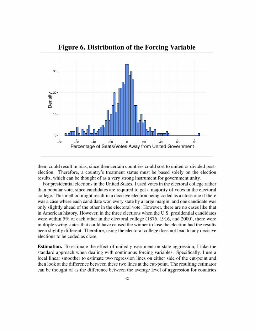
Figure 6. Distribution of the Forcing Variable

0

10

20

30

−80 −60 −40 −20 0 20 40 60 80Percentage of Seats/Votes Away from United Government

Den

sity

them could result in bias, since then certain countries could sort to united or divided post-election. Therefore, a country’s treatment status must be based solely on the electionresults, which can be thought of as a very strong instrument for government unity.

For presidential elections in the United States, I used votes in the electoral college ratherthan popular vote, since candidates are required to get a majority of votes in the electoralcollege. This method might result in a decisive election being coded as a close one if therewas a case where each candidate won every state by a large margin, and one candidate wasonly slightly ahead of the other in the electoral vote. However, there are no cases like thatin American history. However, in the three elections when the U.S. presidential candidateswere within 5% of each other in the electoral college (1876, 1916, and 2000), there weremultiple swing states that could have caused the winner to lose the election had the resultsbeen slightly different. Therefore, using the electoral college does not lead to any decisiveelections to be coded as close.

Estimation. To estimate the effect of united government on state aggression, I take thestandard approach when dealing with continuous forcing variables. Specifically, I use alocal linear smoother to estimate two regression lines on either side of the cut-point andthen look at the difference between these two lines at the cut-point. The resulting estimatorcan be thought of as the difference between the average level of aggression for countries

42

with united governments and the average level of aggression for countries with dividedgovernments, as it is defined exactly at the cut-point. To carry out this estimation, I usethe “rdrobust” software developed by Calonico, Cattaneo, and Titiunik (2014), which pro-duces bias-corrected estimates with robust standard errors. Their software also calculatesthe optimal bandwidth to minimize the mean-squared error, which is the standard crite-rion for bandwidth selection. To illustrate the treatment effect, I also create the normalregression discontinuity graphs with bootstrapped standard errors. These graphs do notshow the bias correction, but the results are very similar to the bias-corrected estimates.To make this estimator doubly robust, I use the change in aggression for each country(difference-in-differences) rather than just its unadjusted aggression level.

Measuring Aggression. Similar to past studies (Gartzke 2007; Dafoe, Oneal, and Rus-sett 2013), I measure aggression using the number of militarized interstate disputes (MIDs)that a country initiates. These disputes are instances where states explicitly threaten, dis-play, or use force against other countries (Ghosn, Palmer, Bremer 2004). Furthermore, Idistinguish between high-level disputes that involve the use of force and low-level disputesthat do not. This distinction is important because there are theoretical reasons to expectunited government to have a larger effect on high-level disputes than low-level disputes.Since the amount of time between elections varies across cases, I also divide the number ofdisputes in each case by the total number of years that the government remained in power.Thus, the unit of measurement is disputes-per-year for each country.

Checking for Balance. Before moving on to the main results, we can check whether theestimator identifies systematic imbalances for any important covariate. Figure 7 shows thebalance tests for a number of key pre-treatment characteristics. Overall, the balance looksbetter than what we would expect in a typical randomized experiment, where p-valueswould be normally distributed between 0 and 1. The only variable that is close to beingimbalanced is low-level disputes, primarily because the bare non-qualifiers initiated sur-prisingly few low-level disputes in the previous period. The two groups were comparableon high-level disputes, which is the main outcome of interest in this study. Moreover,when high and low-level disputes are combined, the two groups are fairly well balanced(p=0.24).

SECTION 4: FINDINGSFigure 8 tracks the aggression levels of the countries that were within 2% of the cut-

point. This sample consists of 33 countries that were barely united and 33 that were barelydivided. The graph shows that the barely united countries initiated many more disputesthan the barely divided ones, even though the two groups had similar aggression levels inthe prior period. On average, the barely united countries initiated about 0.38 disputes per

43

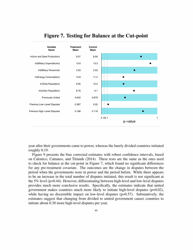
Figure 7. Testing for Balance at the Cut-point

VariableName

TreatmentMean

ControlMean

ln(Iron and Steel Production) 9.07 8.95 ●

ln(Military Expenditures) 13.6 13.3 ●

ln(Military Personnel) 4.53 4.53 ●

ln(Energy Consumption) 10.8 11.4 ●

ln(Total Population) 9.95 10.4 ●

ln(Urban Population) 8.76 9.1 ●

Previously United 0.642 0.679 ●

Previous Low−Level Disputes 0.367 0.02 ●

Previous High−Level Disputes 0.168 0.118 ●

0 .05.1 1p−value

year after their governments came to power, whereas the barely divided countries initiatedroughly 0.19.

Figure 9 presents the bias corrected estimates with robust confidence intervals, basedon Calonico, Cattaneo, and Titiunik (2014). These tests are the same as the ones usedto check for balance at the cut-point in Figure 7, which found no significant differencesfor any pre-treatment covariate. The outcomes are the change in disputes between theperiod when the governments were in power and the period before. While there appearsto be an increase in the total number of disputes initiated, this result is not significant atthe 5% level (p=0.44). However, differentiating between high-level and low-level disputesprovides much more conclusive results. Specifically, the estimates indicate that unitedgovernment makes countries much more likely to initiate high-level disputes (p=0.02),while having no discernible impact on low-level disputes (p=0.57). Substantively, theestimates suggest that changing from divided to united government causes countries toinitiate about 0.38 more high-level disputes per year.

44

Figure 8. Change in Aggression for Barely Unitedand Barely Divided Countries

Barely UnitedBarely Divided

Elec

tion

0

1

2

3

4

5

6

Previous Period Period in PowerTime

Milit

ary

Dis

pute

s In

itiat

ed

Note: This graph shows the disputes initiated by countries that were within2% of being united or divided.

Individual Countries. To illustrate which countries are most responsible for influencingthe results, I have provided a standard regression discontinuity graph (Figure 10) wherethe observations close to the cut-point are labeled. Specifically, I labelled any country thathad at least one high level military dispute and fell within the bandwidth (h= 1.83%). Thisbandwidth was selected using the algorithm provided by Calonico, Cattaneo, and Titiunik(2014).The graph shows that the United States is playing an important role in influencingthe results, but no other country stands out. In fact, the results are almost significant forjust the United States (p=0.053).

45

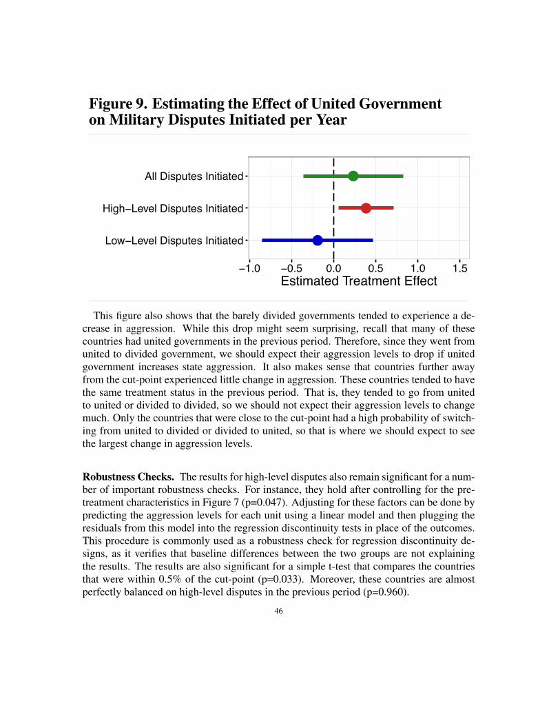
Figure 9. Estimating the Effect of United Governmenton Military Disputes Initiated per Year

●

●

●Low−Level Disputes Initiated

High−Level Disputes Initiated

All Disputes Initiated

−1.0 −0.5 0.0 0.5 1.0 1.5Estimated Treatment Effect

This figure also shows that the barely divided governments tended to experience a de-crease in aggression. While this drop might seem surprising, recall that many of thesecountries had united governments in the previous period. Therefore, since they went fromunited to divided government, we should expect their aggression levels to drop if unitedgovernment increases state aggression. It also makes sense that countries further awayfrom the cut-point experienced little change in aggression. These countries tended to havethe same treatment status in the previous period. That is, they tended to go from unitedto united or divided to divided, so we should not expect their aggression levels to changemuch. Only the countries that were close to the cut-point had a high probability of switch-ing from united to divided or divided to united, so that is where we should expect to seethe largest change in aggression levels.

Robustness Checks. The results for high-level disputes also remain significant for a num-ber of important robustness checks. For instance, they hold after controlling for the pre-treatment characteristics in Figure 7 (p=0.047). Adjusting for these factors can be done bypredicting the aggression levels for each unit using a linear model and then plugging theresiduals from this model into the regression discontinuity tests in place of the outcomes.This procedure is commonly used as a robustness check for regression discontinuity de-signs, as it verifies that baseline differences between the two groups are not explainingthe results. The results are also significant for a simple t-test that compares the countriesthat were within 0.5% of the cut-point (p=0.033). Moreover, these countries are almostperfectly balanced on high-level disputes in the previous period (p=0.960).

46

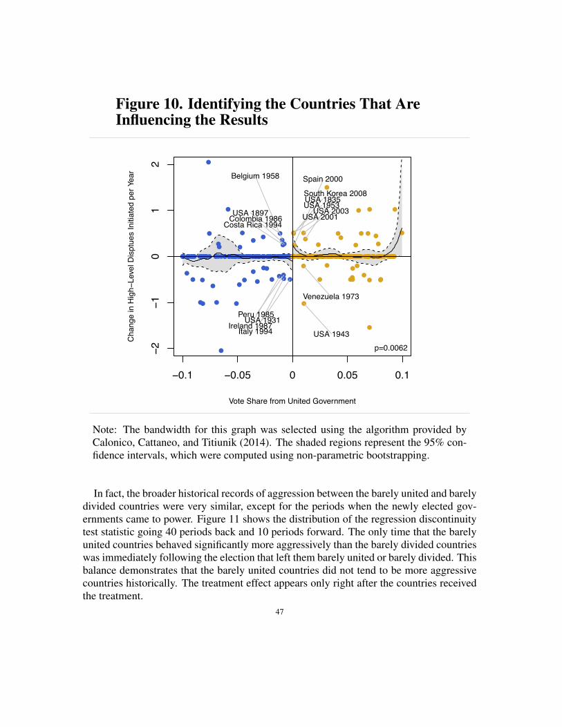
Figure 10. Identifying the Countries That AreInfluencing the Results

●

●

●

●●

●

●

●

●

●

●

●

●

●

●● ●

●

●●

●

●● ●●●

● ●

● ●●

●

●● ●●●

●

●

● ● ●● ● ●●●● ●

●

●

●● ●● ●● ●●

●

●●

●

● ●●● ● ●●● ●●● ●●

●

● ●●

●● ● ●

●

●

●

● ●

●

● ●● ● ●●● ●●● ● ●●

●

● ●● ●● ●

●

●●

●

● ● ●● ●●

●

●

●

●

●

●

−2−1

01

2

Vote Share from United Government

Cha

nge

in H

igh−

Leve

l Dis

ptue

s In

itiat

ed p

er Y

ear

●

●

●●

● ●

● ●

●●

● ●●

●

●

●

● ●

●

●

●

●

●

●●●

●●

●

●

●

●

● ●● ● ●● ●●●● ● ●●

●●

●● ●●● ●● ●● ●●●

●

● ●●

●

●

●

●

●● ● ●● ●●●●

●

●●●

●

●●

●●

●●●● ●●● ● ●● ● ● ●●● ● ●● ●● ●●● ●● ●●●●●

●●● ●● ●●● ●

●

● ●●●●●

●

●

●

●●

●

●

●

●

●

●

●

●

●

●● ●

●

●●

●

●● ●●●

● ●

● ●●

●

●● ●●●

●

●

● ● ●● ● ●●●● ●

●

●

●● ●● ●● ●●

●

●●

●

● ●●● ● ●●● ●●● ●●

●

● ●

●

●● ● ●

●

●

●

● ●

●

● ●● ● ●●● ●●● ● ●●

●

● ●● ●● ●

●

●●

●

● ● ●● ●●

●

●

●

●

●

●

●

●

●●

● ●

● ●

●●

● ●●

●

●

●

● ●

●

●

●

●

●

●●●

●●

●

●

●

●

● ●● ● ●● ●●●● ● ●●

●

●

●● ●●● ●● ●● ●●●

●

● ●●

●

●

●

●

●● ● ●● ●●●●

●

●●●

●

●●

●●

●●●● ●●● ● ●● ● ● ●●● ● ●● ●● ●●● ●● ●●●

●●

●●● ●● ●●● ●

●

● ●●●●●

−0.1 −0.05 0 0.05 0.1

p=0.0062

USA 2003USA 2001USA 1953

USA 1943USA 1931

USA 1897USA 1835

Colombia 1986

Peru 1985

Venezuela 1973

Costa Rica 1994

Ireland 1987

South Korea 2008

Belgium 1958

Italy 1994

Spain 2000

Note: The bandwidth for this graph was selected using the algorithm provided byCalonico, Cattaneo, and Titiunik (2014). The shaded regions represent the 95% con-fidence intervals, which were computed using non-parametric bootstrapping.

In fact, the broader historical records of aggression between the barely united and barelydivided countries were very similar, except for the periods when the newly elected gov-ernments came to power. Figure 11 shows the distribution of the regression discontinuitytest statistic going 40 periods back and 10 periods forward. The only time that the barelyunited countries behaved significantly more aggressively than the barely divided countrieswas immediately following the election that left them barely united or barely divided. Thisbalance demonstrates that the barely united countries did not tend to be more aggressivecountries historically. The treatment effect appears only right after the countries receivedthe treatment.

47

Figure 11. Testing for a Treatment Effect over Time

Elec

tion

−1

0

1

2

−40 −30 −20 −10 0 10Period

Test

Sta

tistic

SECTION 5: DISCUSSIONThis study finds strong evidence that united government increases the likelihood of

interstate conflict. While the results are fairly straightforward to interpret, there are severalimportant points that are worth keeping in mind about this finding.

First, it does not imply that increasing government unity will tend to make state ag-gression more likely for all types of countries. After all, the countries considered in thisstudy are all democracies. Whether an exogenous increase in government unity wouldhave a similar effect on an autocratic regime is a different question. In fact, the literatureon diversionary war theory suggests that government unity may actually decrease aggres-sion for non-democracies, since it alleviates leaders’ need to use international rivalry tostrengthen their support at home (Oakes 2006). Another group of countries that may re-spond differently are democracies that are experiencing severe economic downturns, astheir leaders may find military action an easier way to win public support than trying topass legislation through a divided government (Brulé 2006). Thus, it seems very unlikelythat government unity increases state aggression under all conditions. The results of thisstudy simply indicate that democracies typically tend to resort to military force more oftenwhen their governments are barely united.

Second, these findings suggest that opposition parties play an important role in con-straining democratic aggression. In fact, we might expect that democratic peace theory

48

will be more likely to hold for democracies with divided governments. Of course, otherfactors may also contribute to the democratic peace, such as liberal norms, open interna-tional markets, and better information about government capabilities and intentions. How-ever, the role of strong opposition parties in constraining democratic aggression should notbe overlooked. As this study shows, foreign policy is more constrained when oppositionparties possess greater institutional power.

Third, these results suggest that the political opposition often opposes the military am-bitions of leaders. This suggests that opposition parties may be concerned about the “Rally’Round the Flag” effect that could strengthen the power of the leader’s party at their ex-pense. Thus, the results might be best understood not simply as a one-way effect of do-mestic politics on international relations. Rather, they may involve the interaction betweenthese two realms. Events at the international level can affect outcomes at the domesticlevel, which means that domestic actors could have incentives to shape those events andthereby influence international relations.

CONCLUSIONWhile united government may lead to positive outcomes at the domestic level, scholars

have long suspected that it has adverse effects on international relations. Past researchon this topic provided compelling reasons for why institutional unity might matter, butdifferent statistical models led to competing conclusions about the true effect of unitedgovernment on interstate conflict. This study shed new light on the debate by taking ad-vantage of a natural experiment where united government was assigned to countries as-ifrandomly. The results provide strong evidence that united government increases the like-lihood of state aggression, especially when it comes to high level-disputes.

This study should make policymakers and the general public much more wary about thepotential for unnecessary conflicts when government is united. At the same time, it shoulddraw attention to the possibility that divided governments might avoid some necessaryconflicts, since opposition parties may wrongly oppose aggressive foreign policy movesthat would actually be in the best interests of their countries. This danger seems to beespecially concerning for the United States, which influences the results more than anyother country. In sum, Americans should be acutely aware of the potential for domesticpolitics to have a negative impact on foreign policy.

49

REFERENCESBarbieri, Katherine, Omar M. G. Keshk, and Brian Pollins. 2009. “Trading Data: Eval-

uating our Assumptions and Coding Rules.” Conflict Management and Peace Science.26(5): 471-491.

Bernecker, Andreas. 2014. “Divided We Reform? Evidence from US Welfare Policies.”Working Paper.

Bertoli, Andrew. 2015. “Nationalism and Interstate Conflict: A Regression DiscontinuityAnalysis.” Working Paper.

Bommarito, Michael J., Daniel Martin Katz, and Paul Poast. 2011. “World Treaty Index.”Broockman, David E. 2009. “Do Congressional Candidates Have Reverse Coattails? Evi-

dence from a Regression Discontinuity Design.” Political Analysis 17(4), 418-34.Brulé, David. 2006. “Congressional Opposition, the Economy, and US Dispute Initiation,

1946-2000.” Journal of Conflict Resolution 50(4): 463-483.Calonico, Sebastian, Matias D. Cattaneo, and Rocio Titiunik. 2014. “Robust Nonparamet-

ric Confidence Intervals for Regression-Discontinuity Designs.” Econometrica 82(6):2295-2326.

Calonico, Sebastian, Matias D. Cattaneo, and Rocio Titiunik. 2014. “rdrobust: An RPackage for Robust Inference in Regression-Discontinuity Designs.” preparation forJournal of Statistical Software.

Campbell, James E., and Joe A. Sumners. 1990. “Presidential Coattails in Senate Elec-tions.” American Political Science Review 84(2): 513-524.

Cederman, Lars-Erik and T. Camber Warren and Didier Sornette. 2011. “Testing Clause-witz: Nationalism, Mass Mobilization, and the Severity of War.” International Organi-zation 65(4), 605-38.

Clark, David H. 2000. “Agreeing to disagree: Domestic institutional congruence and USdispute behavior.” Political Research Quarterly 53(2): 375-400.

Clark, David H., and Timothy Nordstrom. 2005. “Democratic Variants and DemocraticVariance: How Domestic Constraints Shape Interstate Conflict.” Journal of Politics67(1): 250-270.

Dafoe, Allan, John R. Oneal, and Bruce Russett. 2013. The Democratic Peace: Weighingthe Evidence and Cautious Inference. International Studies Quarterly 57(1), 201-14.

Dunning, Thad. Natural Experiments in the Social Sciences: A Design-Based Approach.Cambridge University Press: 2012.

Eggers, Andrew, Anthony Fowler, Jens Hainmueller, Andrew B. Hall, and James M. Sny-der Jr. 2014. “On the validity of the regression discontinuity design for estimatingelectoral effects: New evidence from over 40,000 close races.” Formerly MIT PoliticalScience Department Working Paper Series 2013-26.

Eggers, A., and J. Hainmueller. 2009. “MP’s for Sale: Returns to Office in Postwar BritishPolitics.” American Political Science Review 103(4): 513-543.

50

French, Bill and John Bradshaw. “Ending the Endless War An Incremental Approach toRepealing the 2001 AUMF.” Published by the National Security Network.

Gartzke, Erik. 2007. “The Capitalist Peace.” American Journal of Political Science 51(1),166-91.

Gerber, Alan S., Daniel P. Kessler, and Marc Meredith. 2011. “The Persuasive Effectsof Direct Mail: A Regression Discontinuity Based Approach.” The Journal of Politics73(01), 140-55.

Ghosn, Faten, Glenn Palmer, and Stuart A. Bremer. 2004. “The MID3 Data Set, 1993-2001: Procedures, Coding Rules, and Description.” Conflict Management and PeaceScience 21(2), 133-54.

Gowa, Joanne. 1998. “Politics at the Water’s Edge: Parties, Voters, and the Use of ForceAbroad.” International Organization 52(2): 307-324.

Howell, William G. and Jon C. Pevehouse. 2005. “Presidents, Congress, and the Use ofForce.” International Organization 59(1): 209-232.

Leblang, David, and Steve Chan. 2003. “Explaining Wars Fought by Established Democ-racies: Do Institutional Constraints Matter?” Political Research Quarterly 56(4): 385-400.

Lee, David S. 2008. Randomized Experiments from Non-Random Selection in US HouseElections. Journal of Econometrics 142(2), 675-697.

Mueller, John E. 1970. “Presidential Popularity from Truman to Johnson.” AmericanPolitical Science Review 64(1): 18-34.

Nohlen, Dieter, ed. 2005. Elections in the Americas: A Data Handbook. OUP Oxford.Nohlen, Dieter, Florian Grotz, and Christof Hartmann, eds. 2001. Elections in Asia and

the Pacific: A Data Handbook. Oxford University Press.Nohlen, Dieter, and Philip Stöver, eds. 2010. Elections in Europe: A Data Handbook.

OUP Oxford.Nohlen, Dieter, Bernard Thibaut, and Michael Krennerich, eds. 1999. Elections in Africa:

A Data Handbook. OUP Oxford.Oakes, Amy. 2006. “Diversionary war and Argentina’s invasion of the Falkland Islands.”

Security Studies 15(3): 431-463.Oneal, John R., and Anna Lillian Bryan. 1995. “The Rally ’Round the Flag Effect in US

Foreign Policy Crises, 1950-1985.” Political Behavior 17(4): 379-401.Pevehouse, Jon C., Timothy Nordstrom, and Kevin Warnke. 2004. “The COW-2 Inter-

national Organizations Dataset Version 2.0.” Conflict Management and Peace Science21:101-119.

Marshall, Monty G., Ted Robert Gurr, and Keith Jaggers. 2013. “Polity ? Project: PoliticalRegime Characteristics and Transitions, 1800-2012.” Arlington: Polity IV Project.

Rosato, Sebastian. 2003. “The Flawed Logic of Democratic Peace Theory.” AmericanPolitical Science Review 97(04): 585-602.

51

Samii, Cyrus. 2013. “Perils or Promise of Ethnic Integration? Evidence from a Hard Casein Burundi.” American Political Science Review 107(03), 558-73.

Schrock-Jacobson, Gretchen. 2012. “The Violent Consequences of the Nation: National-ism and the Initiation of Interstate War.” Journal of Conflict Resolution 56(5), 825-52.

Schultz, Kenneth A. 1999. “Do Democratic Institutions Constrain or Inform? ContrastingTwo Institutional Perspectives on Democracy and War.” International Organization53(2): 233-266.

Titiunik, Rocio. 2009. “Incumbency Advantage in Brazil: Evidence from MunicipalMayor Elections.” University of California-Berkeley, mimeo.

Tsebelis, George. 1995. “Decision Making in Political Systems: Veto Players in Presi-dentialism, Parliamentarism, Multicameralism and Multipartyism.” British Journal ofPolitical Science 25(3): 289-325.

Voeten, Erik. 2013. “Does Participation in International Organizations Increase Coopera-tion?” The Review of International Organizations 8(3), 1-24.

52

Regression Discontinuity in Practice: Solving

Common Problems in Applied Research

Andrew Bertoli

ABSTRACT. Although regression discontinuity (RD) is a very simple research design intheory, many applications are riddled with subtle complexities, even when treatment as-signment is random close to the cut-point. In this paper, I examine three of the most com-mon problems for regression discontinuity designs: (1) variation in competitiveness acrossstrata, (2) units that appear in the sample multiple times, and (3) independent variables ofinterest that are not actually assigned by the RD. In each case, I explain the problem for-mally, offer straightforward solutions, and illustrate the main points with simulations andreal-world data. To increase clarity, I treat regression discontinuity as a natural experimentin a narrow window around the cut-point. While this approach differs from the more stan-dard practice of taking units’ scores as fixed and estimating the difference at the cut-pointusing two regression lines, I show that the two approaches are very similar mathematically.

Over the last decade, regression discontinuity (RD) has gained popularity in many sci-entific fields. Not only is it one of the most trusted tools of causal inference short of anexperiment (Bernardi and Skoufias 2004; Green et al., 2009), but its simplicity allowsresearchers to present their findings to other scholars and the general public much moreeffectively (Hopkins and McCabe 2012; Hall 2015). Given its virtues, the popularity ofthe regression discontinuity design is likely to continue to grow for the foreseeable future,especially considering the prevalence of scoring systems with cut-points. In recent years,it has even spread to fields like sociology (Rao, Yue, and Ingram 2011; Legewie 2013;Bernardi 2014), international relations (Voeten 2013), peace and conflict studies (Crost,Felter, and Johnston 2014), and criminology (Chen and Shapiro 2007; Vollaard 2009).

But despite RD’s simple and intuitive nature, applications often face subtle problemsthat can pose serious threats to inference. The concern that tends to receive the most atten-tion is that certain units close to the cut-point may be able to manipulate their scores andsort into the treatment or control groups (Imbens and Lemieux 2008; Caughey and Sekhon2011; Eggers et al. 2014). However, even when units cannot sort, other complications canstill occur that are just as problematic. These issues usually arise either from the complexrules of the scoring system or because researchers want to make certain comparisons thatare not necessarily guaranteed to be valid by the RD.

While applied researchers have made important progress in addressing these problems,there are cases where they have confused the issues, sometimes simply because theywanted to avoid undesired complexity in their articles. No doubt, students hoping to learn

53

from past examples of RD could easily be misguided by the choices made in some of themost important applications. Unfortunately, there have only been a few attempts to clarifyand resolve the complications that can occur in real world situations (Keele and Titiu-nik 2014), and some of the most widespread issues have not been explored in scholarlywriting.

In this essay, I investigate three of the most important problems that arise in applied RD,all of which have been largely unaddressed by methodologists. The first occurs when unitsare organized into strata that vary in terms of their competitiveness. For instance, the unitscould be candidates running in different districts, and the districts could vary in terms ofnumber of candidates with a realistic chance of winning. In these cases, researchers mustbe careful which units they include in their sample, or else they risk inducing bias. Thesecond problem occurs when units appear in the sample multiple times, such as whenstudents retake a test or candidates rerun for office. This scenario can cause some units tohave multiple scores and possibly sort from one side of the cut-point to the other. The thirdarises when the independent variable of interest is not actually assigned by the RD. Forinstance, researchers might want to estimate how the likelihood of international conflictchanges when a woman barely defeats a man in an election for head-of-state, even thoughgender is a basic human characteristic that was never itself randomized to politicians. Thisissue can make it difficult to interpret the treatment effect.

To help clarify these problems, I treat regression discontinuity as a natural experimentwhere the treatment is assigned randomly to units within a certain distance of the cut-point(Cattaneo, Frandsen, and Titiunik 2014). This approach differs from the more commonpractice of treating units’ scores as fixed and estimating the difference at the cut-pointwith two regression lines. However, in the next section I show that although these twoapproaches are conceptually very different, they are extremely similar mathematically.Their only major difference is that the continuity approach controls for the score. Bydoing so, the continuity approach has an important advantage. However, it can also makeit harder to identify fundamental design problems that are easier to see when using thenatural experiment approach. A major advantage of the natural experiment setup is thatit prompts researchers to consider whether all units have roughly the same probability oftreatment assignment close to the cut-point.

SECTION 1: THE BASICS OF REGRESSION DISCONTINUITY

Regression discontinuity is a quasi-experimental research design that estimates causaleffects by exploiting scoring systems with important thresholds. The classic example isan exam where every student who scores above a cut-point receives an award and everystudents who scores below does not (Thistlethwaite and Campbell 1960). The idea is thatreceiving the award should be close to random for students who barely made or barely

54

missed the cutoff. Thus, the cut-point creates a source of exogeneity that gives researchersa natural experiment.

In many cases, all of the units that score above the threshold will receive the treatment,while all of the units that score below do not. These situations are referred to as sharp RDs.However, this clean set-up is not always necessary. We can still estimate the causal effectsif some of the units that surpassed the cut-point did not receive the treatment or some unitsthat fell short did. The key is that scoring above the cut-point cannot lower any unit’sprobability of receiving the treatment, and it must increase the probability that at leastsome units got the treatment. In these situations, surpassing the cut-point can be thoughtof as receiving an instrument that increases the probability of treatment assignment forat least some units. These cases are called fuzzy RDs, and they can be analyzed using acombination of regression discontinuity and instrumental variable techniques.

To make this paper more accessible to readers, I write out the notation in terms ofthe conventional (sharp) RD design where all units to the right of the cut-point get thetreatment and all units to the left do not. However, the main points of this paper carry overto fuzzy RDs with the intention-to-treat estimator, since all fuzzy RDs are sharp RDs if wetake the instrument to be our treatment of interest.

There are two ways that researchers analyze regression discontinuities. I describe eachof them below and then discuss their similarities and differences.

The Natural Experiment Set-up. This approach treats regression discontinuity as a natu-ral experiment where the treatment is assigned randomly to units within a certain distanceof the cut-point. Under this set-up, analysis is very straightforward. First, researchers mustchoose a size for their regression discontinuity window. Ideally, they make this decisionprior to looking at the outcomes, and they are normally expected to report the results forother reasonable window choices as a robustness check. Next, researchers focus their at-tention on the units inside the RD window, excluding the others so that they do not effectthe results. This move is valid even if it was somewhat random which units ended up in theRD window. It is similar to a situation where units were selected to be in an experiment ina semi-random manner. Which units ended up in the experiment could be taken as fixed,and then internally valid inferences could be drawn about that sample.

Next, the units inside the RD window are treated as though they were part of a realexperiment. The standard notation is as follows. Denote the number of units as n. Unit i’streatment status is Ti 2 {0,1} and its score as Zi. Under the assumption of non-interferencebetween units, each unit has two potential outcomes, one under treatment (Yit) and theother under control (Yic). The parameter that we are interested in is the Local AverageTreatment Effect (LATE), which is written as

tRD = 1n Âi(Yit �Yic)

This parameter is just the average treatment effect for units inside the RD window. If m isthe number of treated units, then the estimator is

55

tRD = 1m ÂiYitTi � 1

n�m ÂiYic(1�Ti)

which is simply the difference in means between the treated and control units inside theRD window. As in a normal experiment, the standard error of this estimator is typicallyapproximated by bootstrapping or by using the formula

ˆSE =q

s2t

m + s2c

n�m

where s2t and s2

c are the estimated variances of the treated and control units. These areeach calculated using the standard sample-to-population variance formula

s2 = 1N�1 Âi(xi � x)2

The p-value can be approximated using the estimated standard error, or it can be com-puted exactly (for the sharp null hypothesis of no treatment effect) by using permutationinference.

As with real experiments, it is usually possible to decrease the standard errors and re-duce bias from baseline differences between the two groups by controlling for covariatesthat are predictive of the outcome. For instance, we could run a regression on the sampleor do difference-in-differences estimation, as is commonly done with experimental data.However, these adjustment methods are usually considered robustness checks rather thanvalid procedures to get the main results. The reason is that allowing researchers to controlfor whatever covariates they want makes it possible for them to manipulate their results sothat they can get lower p-values (Masicampo and Lalande 2012).

However, when analyzing a regression discontinuity, there is one additional reason toconsider performing covariate adjustment that does apply to real experiments. In experi-ments, the treatment is randomized, making the unadjusted difference in means estimatoris unbiased. On the other hand, regression discontinuity gives us two groups that werenot actually randomized. For instance, if we are comparing leaders who won or lost theirelections by less than 100 votes, we should expect the bare winners to differ from the barelosers in small but systematic ways. We might expect the bare winners to be slightly higherquality, wealthier, or smarter than the bare losers, and if we had a large enough sample sizewe would actually be able to pin-point these differences using difference in means tests.

The most direct way to account for these systematic differences is to control for thescore, Z, using some linear or non-parametric model. This step will eliminate small base-line imbalances that result from differences in the score for units on either side of thecut-point, provided that the relationship between the score and outcome is modeled cor-rectly. I will discuss some possible models in the next section, as well as draw connectionsbetween these models and the second regression discontinuity approach.

The Continuity Set-up. Rather than treating regression discontinuity as a localized nat-ural experiment, most researchers include all of the data and use two regression lines toestimate the difference between the average outcomes of treated and control units at the

56

cut-point. By using regression lines, they are treating the scores as fixed rather than ran-dom. The randomness is now in the error terms of the y’s, and the regression lines are theconditional mean functions that estimate the expected value of y across different values ofthe score. I call this approach the continuity set-up. When researchers use it, the majorquestion that they face is how to construct the regression lines. Specifically, they have twokey decisions to make.

One of these decisions is what bandwidth to use. The bandwidth, denoted as h, can bethought of as analogous to the size of the RD window. It specifies how far to the right or leftof each point z to look to compute the value of the regression line at z. For instance, if thebandwidth is set at h = 2, then the value of the regression function at z would be estimatedby using observations that lie between (z-2, z+2). The bandwidth would normally bechosen using an optimal bandwidth selection algorithm like the one provided by Imbensand Kalyanaraman (2011) or Calonico, Cattaneo, and Titiunik (2014).

The other decision that researchers need to make is how to estimate the regression func-tion using the points within the bandwidth. They could simply use the mean of thesepoints (nearest-neighbor smoother) or a weighted mean that discounts observations thefarther they are from z (kernel smoother). They could also run a (new) regression linethrough these points and take the y value at z (they would then repeat this process for ev-ery z to construct their two regression lines). This method is called local regression. Forinstance, they could run weighted or unweighted regression through the points around in(z�h,z+h) for every z (local linear regression), or they could use polynomial regression(local polynomial regression).

But regardless of how they decide to construct their two regression lines, the regressiondiscontinuity estimator is

tRD = E[Y |Z = c+]�E[Y |Z = c�]which is just the difference between the two regression lines at the cut-point. Thus, whencalculating their estimate, they are only focusing on the value of the regression lines at thecut-point, where Z=c. By doing so, they are ignoring all units that are farther than h awayfrom the cut-point. This is why the bandwidth is analogous to the size of the RD window.It specifies how far to the left and right of the cut-point researchers will look to find pointsto estimate the values of the two regression lines at the cut-point.

Comparing the Two RD Approaches. On a conceptual level, the two regression dis-continuity approaches are very different. The natural experiment approach estimates theaverage treatment effect for the units within the RD window. This is a well defined causaleffect provided that the treatment was as-if random for those units. On the other hand, thecontinuity approach estimates the average treatment effect at the cut-point, where no unitsexist. In this sense, there is no sample where this treatment effect is defined, making itradically different than a traditional causal parameter. Moreover, the continuity approachmakes no as-if random assumption, except at the cut-point where there are no units.

57

Nonetheless, the two approaches are very similar mathematically. As mentioned be-fore, the size of the RD window in the natural experiment approach is analogous to thebandwidth in the continuity approach. All points that fall outside the RD window (orbandwidth) have no impact on the results. In the same way, if we take the natural experi-ment approach and control for only the score, how we control for it is analogous to how weconstruct the regression lines in the continuity approach. In fact, as long as the bandwidthequals the size of the RD window and we use the same method to compute the standarderrors, the natural experiment and continuity set-ups will have mathematically equivalentforms.

The parallels are very straightforward. If we take the natural experiment approach andconduct a weighted difference in means test that weights units by their scores, it is math-ematically equivalent to using a kernel smoother in the continuity approach, provided weused the same kernel (or weighting rule) for both approaches. If we take the natural ex-periment approach and run a regression on the sample within the RD window that controlsfor Z and the interaction Z ⇤T , that is equivalent to using local regression linear regression(unweighted) in the continuity approach. If we take the natural experiment approach andcontrol for for Z,Z2, ...,Zk and the interactions Z ⇤T , Z2 ⇤T , ..., Zk ⇤T , that is equivalentto using a local polynomial regression of order k (unweighted) in the continuity approach.

Figure 1 summarizes these relationships graphically, using a study by Voeten (2013) thatlooks at how being elected to the UN Security Council influences countries’ willingness toparticipate in peace keeping missions. Voting for the UN Security Council is sometimesdone through competitive elections, where countries secure a position if they receive atleast 50% of the votes. I set the bandwidth (or size of the RD window) at h = 0.1, or10%, which is close to the optimal bandwidth using the algorithm proposed by Calonico,Cattaneo, and Titiunik (2014). Thus, we are focusing on countries that received between40% and 60% approval. Normally, we would also want to try smaller bandwidths wherethe as-if random assumption is more plausible, especially if we were not controlling forthe score. However, since we are just using this study as an illustrative example, we willfix the bandwidth at 10%.

The figure shows that using the mathematical similarity between the natural experimentand continuity approaches. If we use the natural experiment approach and control for thesystematic discrepancies between the treatment and control groups resulting from smalldifferences in the score, we are really just doing a version of the continuity approach.Which version we are doing simply depends on how we control for the score.

A key point here is the importance of the as-if randomness for both approaches. Allthat the continuity set-up addresses is the bias that can result from units on one side of thecut-point being slightly different than units on the other side due to the small differences intheir score. If certain units are more likely to be in bare winners than others for any reasonother than the small differences in their scores, than the continuity approach is not longerunbiased. For instance, we can live with the fact that candidates that won by less than

58

Figure 1. Similarity of the RD Approaches

Natural Experiment Setup

● ●

●

●●

●

●

●

●

●

●

●

●

●●

●

●

●

02

46

8

Votes from Winning Position on UN Security Council

ln(P

eace

keep

ing

Mis

sion

s)

●●

●

●

●

●

●

●

●

●

●

●

●

●

●

●

●●

●

● ●

●

●

●

●

●

●

●

●

●

●

●

●

●

●

●

●

●

● ● ●●

●

● ●●

●

●

●●

●

●

●●

●

●

●●

●

●

●

●●

●

−30% −20% −10% 0% 10% 20% 30%

Weight Difference in Means

t = 1.999 p = 0.036

Continuity Setup

● ●

●

●●

●

●

●

●

●

●

●

●

●●

●

●

●

02

46

8

Votes from Winning Position on UN Security Council

ln(P

eace

keep

ing

Mis

sion

s)

●●

●

●

●

●

●

●

●

●

●

●

●

●

●

●

●●

●

● ●

●

●

● ●

●

●●

●

●

●

●

●

●

●

●

●●

●

●

●

●●

●

●

●

●

●

●

●

●

●

●

●

●

●

●

●●

●

●●

●

●

−30% −20% −10% 0% 10% 20% 30%

p=0.036

Kernel Smoother

t = 1.999 p = 0.036

● ●

●

●●

●

●

●

●

●

●

●

●

●●

●

●

●

02

46

8

Votes from Winning Position on UN Security Council

ln(P

eace

keep

ing

Mis

sion

s)

●●

●

●

●

●

●

●

●

●

●

●

●

●

●

●

●●

●

● ●

●

●

●

●

●

●

●

●

●

●

●

●

●

●

●

●

●

● ● ●●

●

● ●●

●

●

●●

●

●

●●

●

●

●●

●

●

●

●●

●

−30% −20% −10% 0% 10% 20% 30%

Y = a +b1T +b2Z +b3T ⇤Z

t = 0.4705 p = 0.7

● ●

●

●●

●

●

●

●

●

●

●

●

●●

●

●

●

02

46

8

Votes from Winning Position on UN Security Council

ln(P

eace

keep

ing

Mis

sion

s)

●●

●

●

●

●

●

●

●

●

●

●

●

●

●

●

●●

●

● ●

●

●

● ●

●

●●

●

●

●

●

●

●

●

●

●●

●

●

●

●●

●

●

●

●

●

●

●

●

●

●

●

●

●

●

●●

●

●●

●

●

−30% −20% −10% 0% 10% 20% 30%

p=0.7

Local Linear Regression (Unweighted)

t = 0.4705 p = 0.7

● ●

●

●●

●

●

●

●

●

●

●

●

●●

●

●

●

02

46

8

Votes from Winning Position on UN Security Council

ln(P

eace

keep

ing

Mis

sion

s)

●●

●

●

●

●

●

●

●

●

●

●

●

●

●

●

●●

●

● ●

●

●

●

●

●

●

●

●

●

●

●

●

●

●

●

●

●

● ● ●●

●

● ●●

●

●

●●

●

●

●●

●

●

●●

●

●

●

●●

●

−30% −20% −10% 0% 10% 20% 30%

Y = a +b1T +b2Z +b3Z2 +b4T ⇤Z +b5T ⇤Z2

t =�1.885 p = 0.24

● ●

●

●●

●

●

●

●

●

●

●

●

●●

●

●

●

02

46

8

Votes from Winning Position on UN Security Council

ln(P

eace

keep

ing

Mis

sion

s)

●●

●

●

●

●

●

●

●

●

●

●

●

●

●

●

●●

●

● ●

●

●

● ●

●

●●

●

●

●

●

●

●

●

●

●●

●

●

●

●●

●

●

●

●

●

●

●

●

●

●

●

●

●

●

●●

●

●●

●

●

−30% −20% −10% 0% 10% 20% 30%

p=0.24

Local Polynomial Regression (2nd Order)

t =�1.885 p = 0.24

Note: For the p-values to be equal, they must be bootstrapped, as there are small differ-ences in some of the methods for computing p-values across the approaches.

100 votes might tend to be of slightly higher quality than candidates who lost by less than100 votes. This bias can be eliminated by using the continuity approach, or by taking thenatural experiment approach and controlling the score. However, we cannot live with thesituation where certain units had other advantages that increased their chances of landing

59

in the bare winning group. Of course, if we control for the score, we must also assumethat the model correctly captures the relationship between the score and the outcome.

Now while these two approaches are very similar mathematically, they each have theirown advantages conceptually. In particular, the natural experiment approach is particularlyuseful for thinking about the design. Specifically, we can ask whether units that are veryclose to the cut-point all had roughly the same probability of being treated, or if some unitshad an advantage that cannot be accounted for by controlling for score. This question doesnot make sense in the continuity set-up, as each unit’s score is considered fixed. However,it is an essential question for any regression discontinuity design. It can help researchersidentify major problems and their solutions, as I will illustrate in the next three sections.

SECTION 2: VARIATION IN COMPETITIVENESS ACROSS STRATA

In the simplest RD set-up, units are all grouped together into the same pool, such astest-takers competing for a fixed number of scholarships. In these cases, there is onlyone strata, and all units belong to it. Analysis under this set-up is fairly straightforward.As long as the units around the cut-point could not manipulate their scores in a preciseway, the treatment assignment around the cut-off should be “as-if” random. We shouldnot expect imbalances on factors like gender, wealth, or ideology, since these should bebalanced by the exogeneity of the treatment.

However, many regression discontinuities have more complicated formats where unitsare grouped into strata. For example, RDs that involve elections have units that are groupedinto electoral strata (districts, states, countries, etc.) and the candidates in each stratacompete against each other for office. This format has also appeared in other types of RD,including Van der Klaauw (2002), Niu, Xinchun, and Tienda (2013), and Bertoli (2015a).

The problem is that differences across strata could bias the results if they correlate withthe probability of barely winning or barely losing. Before I lay out this problem formally,let me first illustrate it with an example. Consider an electoral system with two majorparties. Now imagine that a third party decides to run in districts where it believes it has agood chance of winning, and that in many cases it scores close to the cut-point, along withthe other two parties. For these districts where three candidates are in the RD window,the candidates would have roughly a 1/3 chance of barely winning and a 2/3 chance ofbarely losing. Thus, the candidates running in these districts would be more likely to bebare losers. If these candidates differed in systematic ways from the candidates running indistricts with only two candidates in the RD window, the unequal probability of treatmentassignment could bias the results.

This problem can arise anytime the strata vary in terms of their competitiveness. In thesecases, more competitive strata will tend to have more bare losers than less competitivestrata. In the election example, a district with four competitive parties may have three barelosers, whereas a district with two competitive parties can only have one bare loser. Thus,

60

when we combine a sample of bare winners and bare losers in close elections, we wouldexpect the following two observable implications:

(1) The bare loser group should be larger than the bare winner group.

(2) The bare loser group should have more units from competitive districts than thebare-winner group.

We should also expect these problems to worsen as the number of districts with multipleparties close to the cut-point grows.

This source of imbalance will be particularly dangerous if we are trying to estimatesomething like the party incumbency advantage, which many recent studies have tried todo in multi-party systems (Uppal 2009; Titiunik 2009). Bare losers will be more likelyto be running in districts where they are up against multiple rival parties that have a goodchance of winning. Thus, when we look at whether these parties won in their next election,we should expect them to win at lower rates than if they were running against just onecompetitive party. In short, they are more likely to lose this time and more likely to losenext time. The result is that barely losing will appear to be more costly than it really is,causing us to overestimate the incumbency advantage.

Researchers using the continuity approach might argue that their design avoids thisproblem because it estimates the LATE exactly at the cut-point, and the probability of athird place candidate existing at this point rapidly converges to 0 for a continuous run-ning variable. Most importantly, it converges to 0 much faster than the probability forsecond-place candidate being at the cut-point. In other words, while it is very unlikely thatone candidate will lose by exactly one vote, it is far less likely that two candidates fromthe same district will both lose by exactly one vote. Thus, the influence of third-placecandidates should be negligible at the cut-point.

However, in RD applications, inferences about the cut-point are always drawn from thedata around the cut-point, and multiple bare losers from one strata can influence the results.As I will show momentarily, whether controlling for Z helps eliminate this bias depends onwhether the model correctly captures the way that the third-place units’ influence decreasesthe closer they get to the cut-point. If it overestimates or underestimates the rate at whichtheir influence changes, then the regression function can be severely biased at the cut-point.

Before we get to that, let us first write this problem out formally using the simple naturalexperiment set-up. The estimator we will use is tFull , which will be the difference in meansestimator for all units that fall in the RD window. We will assume for now that there canonly be one winner, as in electoral cases. Then our estimator is written as

tFull =1m Ân

i=1YitTi � 1n�m Ân

i=1Yic(1�Ti)

61

Let Ci denote the number of units that are in the RD window in Unit i’s strata. SoI(Ci = k) is an indicator variable that equals 1 if there are k units in the RD window inUnit i’s strata, and equals 0 otherwise. Moreover, let q be the maximum number of unitsin the RD window in any strata. Then tFull can be decomposed as follows

tFull =1m Ân

i=1YitI(Ci = 2)� 1n�m Ân

i=1YicI(Ci = 2)+

1m Ân

i=1YitI(Ci = 3)� 1n�m Ân

i=1YicI(Ci = 3)+...1m Ân

i=1YitI(Ci = q)� 1n�m Ân

i=1YicI(Ci = q)

Now note that for a strata with k units in the RD window, the probability of barely winningis P(Ti = 1) = 1

k and the probability of barely losing is P(Ti = 0) = k�1k . Using these

expression, we can write out the expected value of our estimator as follows:

E[tFull] =1m · 1

2 Âni=1YitI(Ci = 2)� 1

n�m · 12 Ân

i=1YicI(Ci = 2)+

1m · 1

3 Âni=1YitI(Ci = 3)� 1

n�m · 23 Ân

i=1YicI(Ci = 3)+...1m · 1

q Âni=1YitI(Ci = q)� 1

n�m · q�1q Ân

i=1YicI(Ci = q)which reduces to

E[tFull] =1n Ân

i=1[YitI(Ci = 2)+YitI(Ci = 3)/(3/2)+ ...+YitI(Ci = k)/(k/2)]�1n Ân

i=1[YicI(Ci = 2)� (3/2) ·YicI(Ci = 3)� (k/2) ·YicI(Ci = k)]

Of the two terms on the right hand side, the top estimates the average outcome under treat-ment, 1

n Âni=1Yit , and the bottom estimates the average outcome under control, 1

n Âni=1Yic.

However, the estimate of the average outcome under treatment underweights units fromstrata with many units in the RD window, while the estimate for the average outcomeunder control overweights these units.

Now let us examine this problem by looking at legislative elections across a numbercountries. Eggers et al. (2014) compile a dataset that provides the vote shares of the firstthree parties in about 200,000 elections across ten countries, which include two-party andmulti-party systems. In two-party systems, there are only two candidates close to the cut-point in any election, aside from the rare cases where an independent or minor third-partycandidate performs very well. Thus, we should not expect variation in competitivenessacross strata to be a major problem when dealing with two-party systems. Without thisvariation, there should not be many more bare losers than there are bare winners. On thehand, in countries where there are several competitive parties, we should expect third-partycandidates to cause differences in competitiveness across strata, which will lead to a largerbare loser group.

62

0 2 4 6 8

0.0

0.2

0.4

0.6

0.8

1.0

Figure 2: McCrary Sorting Test Results Third Party Competitiveness Increases

Percent of Elections Where There Are 3 Parties Within 2% of Winning

One

Sid

ed p−v

alue

for D

ownw

ard

Sorri

ng

●●

●●

●

United States

Canada

United KingdomGermanyFrance

AustraliaNew Zealand

India

Brazil

Mexico

Sorting Toward the Losing Side

Balanced

Sorting Toward the Winning Side

Figure 2 shows whether there tended to be more bare losers in the countries using theMcCrary sorting test. This test checks for whether there was an overall tendency for unitsto sort to one side of the cut-point or the other. Any such sorting would be a threat toinference, unless it was entirely independent of the potential outcomes. As this figureshows, countries that had more districts with multiple candidates near the cut-point tendedto fail the McCrary sorting test, Specifically, they had more bare losers than we wouldexpect if each candidate was about equally likely to be on one side of the cut-point or theother.

Figure 3 shows that countries that had more districts with multiple candidates near thecut-point also tended to have more imbalance on the competitiveness of district. There

63

0 2 4 6 8

0.0

0.2

0.4

0.6

0.8

1.0

Figure 3: Testing for Imbalance on Competitiveness of District Across Countries

Percent of Elections Where There Are 3 Parties Within 2% of Winning

One

Sid

ed p−v

alue

for S

ortin

g on

Com

petit

ivene

ss

●

●

●

●

United States

CanadaUnited Kingdom

Germany

FranceAustraliaNew Zealand

IndiaBrazilMexico

Bare Losers Are From More Competitive Disticts

Balanced

Bare Winners Are From More Competitive Disticts

Note: p-values values are computed using difference in means tests for the sample ofcandidates that won or lost by less than 2%.

is no imbalance for countries like Australia, France, and New Zealand, where there areonly two competitive parties in close elections. However, the p-values are close to 0 forcounties like India, Mexico, Brazil, and the United Kingdom (which has the largest numberof close elections aside from the United States). For the entire sample, about 2.8% of thebare losing candidates came from competitive districts, compared to about 1.4% of thebare winning candidates. For a t-test in the RD window, the p-value is p ⇡ 1.7 ·10�11.

64

In fact, it is fairly easy to see that this imbalance must exist. Each winner has exactly onecorresponding runner-up. For instance, if the winning party won by 1%, then the runner-up must have lost by 1%. Moreover, both of these units are either from a district withonly two parties close to the cut-point, or they are both from a more competitive districtwith three parties close to the cut-point. Thus, the winners and runner-ups by themselveswill always be balanced on competitiveness of district, since they are a mirror image ofeach other. However, in cases where there is a third-place party in the RD window, thatparty adds an additional unit in that district. When this happens in many districts, theseadditional bare losers will create the imbalance that is evident in Figure 3.

Because the density of third-place candidates decreases the closer we get to the cut-point, our estimator might be unbiased if we control for Z with a model that accuratelycaptures the decreasing influence of third place candidates as they approach the cut-point.In the case of elections with three parties, the influence of third-place parties will actuallydecrease linearly close to the cut-point. For example, imagine that we set the size of theRD window at (-2%,+2%). The score of a third-place candidate in this RD window is(roughly) the minimum of two draws from the random variable Unif(-2%,0%), which hasa linear density (in this case, f (x) =�x/2 for x 2 (�2,0))). Thus, local linear regressioncan substantially reduce bias in the three-party case. The kernel smoother, however, canlead to badly biased results, as it incorrectly models the relationship between Z and com-petitiveness. The nearest-neighbor smoother can also be biased, since it is equivalent to adifference in means test.

While the local linear smoother can help us avoid bias when some strata have three can-didates in the RD window, it cannot resolve cases where some strata have four or morecandidates close to the cut-point. Put simply, these strata will induce a non-linear relation-ship between Z and the influence of additional bare losers. The fourth place candidateswill be distributed f1(x) = 3x2/8 and the third place candidates will be distributed forf2(x) = �3x2/2� 3x for x 2 (�2,0). These distributions are easily derived using orderstatistics formulas. Without the linearly decreasing influence of the additional bare losers,the local linear smoother can be badly biased. For instance, if you take Eggers et al. datasetof roughly 20,000 bare winners and bare losers and add just 91 fourth-place candidates,each of whom scores half-way between -2% and the third-place candidates, the local linearestimator returns significant imbalance on competitiveness of district. While high-orderpolynomial smoothers may be able to capture the non-linear influence of the additionalbare losers to some extent, they will also be more sensitive to noise in the data and have amuch higher variance (Gelman and Imbens 2014).

In short, when strata have varying numbers of units in the RD window, how we controlfor Z matters. It is no longer a robustness check, but a key decision about the designthat can greatly impact the results. In the three-candidate case, we can go from no biaswith a local linear smoother to substantial bias with a kernel or nearest-neighbor smoother.If we add some fourth-place candidates into the dataset, local linear regression will also

65

become biased. Put simply, the additional bare losers make our results highly sensitive toour modeling assumptions.

Since one of the most appealing features of RD is that it tends to be much less sensitiveto how we model the data, we should consider some ways of resolving this problem. Theeasiest solution is just to restrict the analysis to the two units in each strata that were closestto making and closest to missing the cut-point. While this approach involves droppingunits, and therefore losing some information, it maintains balance over strata and time.In other words, the bare winners and bare losers in the election example will be perfectlybalanced on district and year, since every bare winner has a corresponding bare loser.Thus, this procedure creates a blocking scheme that should increase balance in the sample.Researchers can also still adjust for Z and present the normal continuity graphs with tworegression lines that meet at the cut-point. It is just that all units that were not the closestto making or missing the cut-point would be left out of this graph.

The second solution is to reweight units based on their probability of treatment assign-ment given their strata. If Unit i is from a strata with k units in the RD window and jbare winners, then we would give Unit i weight k

n ·k� j

k if it barely won and weight kn ·

jk if

it barely lost. We could then use a difference in means test under the natural experimentset-up. In electoral settings, this estimator would be

tReweightedFull =1

n2/2 Âni=1YitTiI(Ci = 2)� 1

n2/2 Âni=1Yic(1�Ti)I(Ci = 2)+

1n3/3 Ân

i=1YitTiI(Ci = 3)� 12n3/3 Ân

i=1Yic(1�Ti)I(Ci = 3)+...

1nq/q Ân

i=1YitTiI(Ci = q)� 1(q�1)nq/q Ân

i=1Yic(1�Ti)I(Ci = q)

where nk is the number of units from strata with k outcomes close to the cut-point. Thisestimator is easy proven to be unbiased under the as-if random assumption by taking theexpected value of tReweighedFull . W could still control for the score by using weightedregression with this weighting scheme, thus getting the benefits of local linear or localpolynomial regression. By reweighting, this procedure maintains balance across stratawhile also using all of the data in the RD window. The drawback is that researchers canno longer construct the continuity graph, since variation in the units’ weights cannot beeasily represented graphically.

SECTION 3: UNITS THAT REAPPEAR IN THE SAMPLE

There are two versions of the multiple-score problem. The simple version occurs whenunits have outcomes for each scoring round, such that each score is associated with asingle outcome. In these cases, researchers can simply treat every time that a unit receivesa score as a separate observation. The more problematic version arises when each unit hasonly one outcome, meaning that multiple scores will now correspond to single outcome.

66

For instance, if we wanted to estimate how passing an exam influenced the chances thatstudents went to college, we would have a problem if the students could take the exammultiple times. However, there is a fairly straightforward solution to this problem that Iwill discuss in the second half of this section.Unique Outcomes for Every Score. This issue arises for many studies, including (Lee2008), Hainmueller and Kern (2008), Lalive (2008), Lemieux and Milligan (2008), Broock-man (2009), Titiunik (2009), Cellini, Ferreira, and Rothstein (2010), Hall (2014), Eggerset al. (2014), and Bertoli (2015a; 2015b). For example, consider the RD studies thatlook at the incumbency advantage. Their goal is to estimate how winning an election attime t affects a party’s vote share and winning probability at time t + 1. To increase thesample size, these studies look at long historical periods rather than a single election year,treating each election as a separate observation. The units are parties within each district.These parties’ treatment assignment is whether they won, their score is how close theywere to winning, and their outcome is how they did in the next election. One entry in thedataset would be Party k in District i with the treatment assigned at time t and the outcomeassigned at time t +1, another would be the same party and district with the treatment as-signed at t +1 and the outcome assigned at t +2, and so on. Thus, the problem of havingmultiple scores for single outcomes does not arise, but there is still the issue of rerunningunits.

In these cases, the key question is whether the treatment effect in each round influencesthe LATE in future rounds. If there is good reason to believe that it does not, then re-searchers can consider each case where a unit received a score can as a single observation.However, if the treatment assignment in one round affects either who is in the RD windowlater or the size of future individual treatment effects, then researchers need to be morecareful about how they proceed.

Since this issue is probably clearest in the party incumbency advantage literature, I willstick with that example. First, let us assume that treatment assignment is as good as randomwithin a small window around the cut-point. Now imagine that winning an election at timet increases vote share at t +1 by 3 points. This implies that treatment assignment in roundt can affect which units are very close to the cut-point at time t +1, so treatment in earlyrounds affects who is influencing the LATE in later rounds. Furthermore, imagine thatsome units also receive a 5-point bump for winning if they won in the previous round, butthey only experience a 3-point bump if they lost in the previous round. If some of theseunits are in the RD window back-to-back years, then treatment assignment affects bothwho influences the LATE and the size of treatment effects for some units after the firstround.

We can still test the sharp null hypothesis that incumbency has no impact of vote sharein future rounds, since this hypothesis guarantees independence between rounds. How-ever, deriving point estimates and confidence intervals for the LATE is no longer a simplematter. On one hand, there is no longer a single LATE, since both who is close to the

67

cut-point and how large some of the individual treatment effects are in later rounds dependon treatment assignment in earlier rounds. Thus, the LATE is a random variable. Theparameter that we might be interested in estimating is the expected value of the LATE

over all treatment assignments:

Surprisingly, the normal RD procedures give us an unbiased estimate of this value,assuming that the treatment is random within the RD window and we restrict our attentionto the pair of candidates closest to the cut-point. Let T be the treatment assignment vector,which is composed of the treatment assignment vectors in each of the k rounds.

T = T

1

[T

2

[ ...[T

k

Let the number of units per round be denoted by n1,n2

, ...,nk

units, which are also randomvariables that depend on the treatment assignments in previous rounds, with the exceptionof n1. Furthermore, the LATE is a random variable that is the sum of the LATE’s fromeach round, LAT E1, LATE

2

, ..., LATE

K

, where each of these terms is multiplied by thepercentage of units that are coming from that round:

LATE = n1n

LAT E1 +n

2

n

LATE

2

+ ...+ n

k

n

LATE

k

So the parameter we are interested in is

E[LATE] = E[n1n

LAT E1]+E[n

2

n

LATE

2

]+ ...+E[n

k

n

LATE

k

]

The normal RD estimator can also be broken down into the estimates for each round.The estimate for the first round is clearly unbiased under the normal as-if randomnessassumption, since there is no rerunning problem in this round. However, T1 is not onlyone of 2

n12 possible treatment assignments for Round 1, but also one of 2

n12 possible paths

to Round 2, which is selected at random. Moreover, the RD estimate for Round 2 is anunbiased estimator for all possible treatment assignments in Round 2 on that path. So werandomly selected our path to Round 2, and then got an unbiased estimate for Round 2conditional on that path. Similarly, T2 is a randomly selected path to Round 3, and weagain get an unbiased estimate of the LATE in that round conditional on that path. Thispattern continues until we reach the last round.

The result is that the full path from Round 1 to Round k is randomly selected from allpossible paths, and in each round along the way we have an unbiased estimator for theLATE in that round conditional on being on that path. So we have

E[tRD

] = E[n1n

LAT E1 +E[n

2

n

LATE

2

|T1]+ ...+E[n

k

n

LATE

k

|Tk�1, ...,T1]]

The tower property gives us

E[tRD

] = E[n1n

LAT E1]+E[n

2

n

LATE

2

]+ ...+E[n

k

n

LATE

k

]

E[tRD

] = E[LATE]

68

So even when the size of the effects and observations in the RD window depend on thetreatment, we can still estimate an important parameter of interest. It should be noted,however, that we do not have an unbiased estimate of the realized LATE that occurred onthe observed path unconditional on the path, unless that LATE equals E[LATE]. It willalso not necessarily be an unbiased estimate of the realized LATE conditional on the path.For instance, some LATE’s may only come about if the bare winners and losers in the firstround are very different on baseline covariates, and in these cases t

RD

will be biased fromthe chance imbalance early on.

While we can obtain an unbiased point estimate of E[LATE], confidence intervals aremore complicated? Unfortunately, we have no way of determining what the distribution ofthe LATE looks like. We only have unbiased estimates for each round on a randomly de-termined path, but with possible correlation between treatment assignment and the LATEin future rounds. Simulations suggest that the normal RD confidence intervals can bemisleading if the LATE in future rounds is highly dependent on treatment assignment inearlier rounds. Of course, this problem does not apply if we are simply testing the sharpnull hypothesis.

This issue is a major limitation if we care about quantifying the uncertainty of our pointestimate, which is certainly true in the party incumbency literature. In cases like this,where we both care about the confidence interval and believe that treatment assignmentinfluences the LATE in later rounds, it would probably make more sense to take a differentapproach. One option would be to drop every district after it appears in the RD windowonce, which would limit the sample size and change the parameter to a different LATE,but would provide us with a valid confidence interval under the normal RD assumptions.

Only One Outcome for Each Unit. A more complicated scenario arises when units havemultiple scores but only one outcome. In these cases, there are usually units that bothmake and fall short of the cut-point at different times. The problem is that it is not entirelyclear whether they belong in the treatment or control group, or what values of their scoresshould be used.

The most famous application that deals with this problem Eggers and Hainmueller(2009) APSR article “MP’s for Sale: Returns to Office in Postwar British Politics,” whichtests how winning a seat in British Parliament influences wealth at death. To get aroundthe rerunning issue, they count all candidates who won at least once as winners and usetheir scores from their first winning races, while counting all candidates who never wonas losers and using their scores from their best losing races. For instance, a candidate whoran twice and lost with scores {�30%,�2%} would be given the score �2%, and a can-didate who ran four times with scores {�5%,14%,�1%,�4%} would be given the firstwinning score of 14%. Eggers and Hainmueller then use the usual RD procedures on thisnew sample, where each candidate has only one score and outcome. I call the estimatorthat is obtained by these procedures the First-Winning-Best-Losing (FWBL) estimator.

69

While the FWBL estimator ensures that no unit will have multiple scores, it createsseveral other problems. The first is that the expected size of the treatment group will nowbe much larger than the expected size of the control group. This problem occurs becausebare losers can switch to winners by rerunning, but bare winners are immediately fixed asbare winners provided that they did not already win in a previous round.

Thus, there are four types of candidates: (1) candidates who lose on their first attemptsand fall outside the RD window, and who can rerun in later rounds and move right; (2)candidates who lose on their first attempt and fall inside the RD window, and who can alsorerun in later rounds and move right; (3) candidates who win on their first attempts andfall inside the RD window, and who now have fixed scores in the treatment group; and (4)candidates who win on their first attempts and fall outside the RD window, whose scoresare now also fixed at their first winning score. Although the sizes of the bare winner andbare loser groups should be about equal after every candidate’s first run, candidates in thesecond group (bare losers) can rerun and switch to the bare winner group or to the groupof winners who scored outside the RD window. The result is that the bare loser group getsdepleted, with some of their members switching to the bare winning group. While initiallosers in the first group can rerun and replace them, these units are just as likely to be barewinners as bare losers in any future round. Moreover, even if they move up to becomebare losers, they can still sort out of this group by winning an election in a future round.

In short, the more opportunities that candidates have to win, the more likely they are tobe counted as a bare winners and the less likely they are to be counted as bare losers. Thus,within the RD window, treatment should be correlated with the likelihood of rerunning.More specifically, it should be correlated with their probabilities of rerunning after losing,since they become fixed in the sample after their first win. Since a candidate’s probabilityof rerunning after losing is likely to be related to individual resources and determination,there is reason to suspect that the FWBL estimator will be biased in many cases.

There is also another potential source of bias that would arise even if all units were guar-anteed to run the same number of times. Imagine that there are two types of candidates,those who respond to barely losing by working hard and succeeding later, and those whoget frustrated and put little effort into future campaigns. The more resilient candidateswould tend to sort out of the bare loser category in later rounds, whereas their more easilydiscouraged counterparts would lose badly and be counted as bare losers based on theirperformance in the first round. Thus, even if there was a predetermined rule that requiredeach candidate to run exactly two times, the FWBL could be confounded by this addi-tional source of bias. Specifically, we would expect bare losers to be less resilient thanbare winners.

The nature of this bias is fundamentally more problematic than the imbalance on com-petitiveness across strata in Section 2 because a well-chosen smoother cannot eliminatethis type of bias. In the prior example, the influence of the additional bare losers con-verged to 0 at the cut-point, since the probability of multiple candidates from one strata

70

Figure 2: Types of Candidates Based on First Score

Clear LosersCan Sort Rightin Later Rounds

Bare LosersCan Sort Rightin Later Rounds

Bare WinnersFixed As

Bare Winners

Clear WinnersFixed As

Clear Winnersbarely losing rapidly converged to 0 when Z is continuous. Thus, we could eliminatebias if we chose a smoother that accurately captured the relationship between Z and thedecreasing influence of the additional bare losers. However, in this case the influence ofcandidates rerunning does not converge to 0 the closer we get to the cut-point. Candidatesthat lose by one vote would probably be very likely to rerun, and would bias the FWBLestimator if they won in a later election.

One potential solution to this problem is to use a different estimator that is proposed byQuerubin and Snyder (2011) in a similar study. Their study looks at how winning a seatin US Congress affected individual wealth during the mid-nineteenth century. Rather thanlooking at each candidates first win or best loss, they look at the first time each candidateran. Thus, they count any candidate who lost in his first round as a loser, even if he wonand held office in a later round. Their justification for using this estimator is that onlyabout 9% of candidates who lost on their first try attempted to rerun, so very few of theirlosers ended up holding office later.

This estimator can be thought of as an intention-to-treat (ITT) estimator. The idea here isthat a candidate’s outcome on his first try is an instrument for whether he ever held office.Winning on the first attempt guarantees that the candidate would hold office, whereaslosing increases the probability that the candidate would never hold office. Thus, we canthink of the candidates who lost on their first attempt and never held office as compliers,and the candidates who lost on their first attempt but won later as non-compliers. Ofcourse, all units who won on their first attempt are compliers, since they were guaranteedto hold office. Thus, we have an instrument (winning or losing on the first attempt) andone-way non-compliance, making the estimator that Querubin and Snyder use an ITTestimator.

A third approach is just to acknowledge that the outcome in the first round is an instru-ment and proceed with the fuzzy regression discontinuity design. Fuzzy RDs are situa-tions where the cut-point determines who receives an instrument instead of who receivesthe treatment. The Fuzzy RD estimator is the ITT estimator divided by the estimated localcompliance rate, which is defined as the percentage of first-time losing candidates in theRD window who never held office. I denote this parameter as aLAT E . So the estimator is

LAT EFRD = LAT EIT TaLAT E

71

Since aLAT E < 1, this value will have a larger absolute value than the ITT estimator. Aswith any fuzzy RD, the p-value for this estimator is the same as the ITT estimator p-value,which tests whether the instrument has an affect on the outcome.

The difference between the ITT and Fuzzy RD estimators is that the ITT estimatorcaptures the impact of the instrument (succeeding the first time), whereas the Fuzzy RDestimator captures the effect of the treatment (succeeding at some point). In most applica-tions, the Fuzzy RD estimator will probably be preferable, even when the compliance rateis high. Since the p-values from the two approaches are the same, the decision to use oneestimator over the other matters for the size of the effect but not the statistical significanceof the results.

There are two drawbacks of the Fuzzy RD estimator. First, it requires researchers toassume that the exclusion restriction holds. The instrument cannot affect the outcomethrough in any way aside from affecting the likelihood of the treatment. This assumptionmay be invalid in many cases. In the economic returns to office example, we would haveto assume that the candidates’ outcome in their first races do not affect their future wealthexcept in how they change the probability of holding office at some point. This assumptionwould be violated if there were candidates who would win a future election if they barelyfail the first time, and whether they succeeded the first time affects their future wealth. Inthis scenario, their performance on the first run does not affect their probability of holdingoffice, which is 1 regardless of whether they win or lose. However, it does influencetheir outcomes, thus violating the exclusion restriction. It is therefore very important thatresearchers consider whether the exclusion restriction holds before using the Fuzzy RDestimator.

Second, the Fuzzy RD estimator will usually be biased in finite samples, as is normallythe case with instrumental variable estimators. The reason is that we can estimate bothLAT EIT T and aLAT E without bias, but we cannot convert these values into an unbiasedestimate of LAT EIT T

aLAT E. This problem results from the rule in probability that E[A]

E[B] 6= E[AB ] in

general. However, if the sample size were to go to infinity, the variances of the numeratorand denominator would go to 0, giving us an unbiased estimate of the LAT EIT T

aLAT E. Therefore,

the Fuzzy RD estimator is consistent, albeit not unbiased.It is also possible to increase the power of both of the ITT and Fuzzy RD estimators by

disregarding any attempt where a candidate scored below the RD window. In other words,only count an attempt as an attempt if the unit won or scored within the RD window. Thus,any early attempt where a candidate scored below the RD window would not disqualifythat unit from the analysis. This rule will increase the sample size by retaining any can-didate who had a bad early loss but produced a more competitive score later. I call theseestimators the Refined ITT and Refined Fuzzy RD estimators.

72

In Figure 1, I compare the five estimators using a simple simulation. The simulationprocedures are as follows, although the patterns observed here do not depend on the spe-cific details, but will arise anytime the probability of rerunning is correlated with base-line determinants of the outcome. There are four election years, each with 10,000 candi-dates who run against unnamed opponents. Candidates who score above 50% win theirelections, and candidates that score below 50% lose. Each candidate has a quality levelQi ⇠Uni f (0.2,0.8). The vote share for a candidate in any election is Zi = Qi + e , wheree ⇠ Uni f (�0.2,0.2). Every candidate reruns with probability Pi ⇠ Uni f (0,1), and can-didates that drop out are replaced by new candidates. Ti is the treatment indicator whichequals 1 if the candidate ever held office and 0 if not. A candidate’s baseline wealth isBi = 100,000 ·Pi + e⇤, where e⇤ is another random error term. Finally, wealth at death isWi = Bi+10,000 ·Ti. Thus, the treatment effect of holding office is a constant of $10,000,and wealthier candidates are slightly more likely to rerun than poorer candidates.

The left-hand column shows the density of the running variable for each estimator.All densities are smooth around the cut-point except for the FWBL estimator, which weexpected to be discontinuous since bare losers can sort right. The middle column showsthe bias for each estimator as a function of the correlation between the baseline outcomeand the probability of rerunning. As expected, the FWBL estimator is substantially biased,since wealthier candidates are more likely to rerun and become bare winners if we use theirfirst-winning or best-losing vote share. The Fuzzy RD and Refined Fuzzy RD estimatorsare also biased, even though the exclusion restriction holds in this example. The othertwo estimators perform very well, although they focus on the intention to treat effect (orthe effect of winning the first time). The third column presents the standard errors foreach estimator. The standard errors for the Refined ITT and Fuzzy RD and estimators areslightly lower than the standard errors for the unrefined estimators, since these estimatorsincrease the sample size.

It should be noted, however, that this simulation may not capture what is happeningin Hainmueller’s and Eggers’s study. It depends on the extent to which the probabilityof rerunning correlates with wealth, and they only have a measure of wealth at the timeof each candidate’s death. Querubin and Snyder do have an estimate of baseline wealth.However, very few of their candidates ever won after losing the first-time, so the compli-ance rate is too large to distinguish between these four types of estimators using their data.Thus, it is difficult to illustrate this problem with a real-world example. However, thereare clear theoretical reasons to believe that the FWBL estimator will provide misleadingresults in cases where the compliance rate is lower (many units win after their first loss)and their is a strong correlation between the outcome and the probability of rerunning, andthe simulation illustrates the problem very clearly.

73

Figure 4: Comparing Estimators with a Simulation

0.0

0.5

1.0

1.5

2.0

0.00.10.20.30.40.50.60.70.80.91.0Vote ShareFi

rst−

Win

ning−B

est−

Losi

ng E

stim

ator

Den

sity

Distribution of the Forcing Varible

0.0

0.5

1.0

1.5

0.00.10.20.30.40.50.60.70.80.91.0Vote Share

Inte

ntio

n−to−T

reat

Est

imat

or

Den

sity

0

1

2

3

0.0 0.1 0.2 0.3 0.4 0.5 0.6 0.7 0.8 0.9 1.0Vote Share

Ref

ined

Inte

ntio

n−To−T

reat

Est

imat

or

Den

sity

0.0

0.5

1.0

1.5

0.00.10.20.30.40.50.60.70.80.91.0Vote Share

Fuzz

y R

DD

Est

imat

or

Den

sity

0

1

2

3

0.0 0.1 0.2 0.3 0.4 0.5 0.6 0.7 0.8 0.9 1.0Vote Share

Ref

ined

Fuz

zy R

DD

Est

imat

or

Den

sity

−10000−5000

05000

10000

0.25 0.50 0.75Correlation Between Rerun Probability

and Baseline Outcome

Bias

Bias of the Estimator

−10000

−5000

0

5000

10000

0.25 0.50 0.75Correlation Between Rerun Probability

and Baseline Outcome

Bias

−10000

−5000

0

5000

10000

0.25 0.50 0.75Correlation Between Rerun Probability

and Baseline Outcome

Bias

−10000

−5000

0

5000

10000

0.25 0.50 0.75Correlation Between Rerun Probability

and Baseline Outcome

Bias

−10000

−5000

0

5000

10000

0.25 0.50 0.75Correlation Between Rerun Probability

and Baseline Outcome

Bias

010002000300040005000

0.25 0.50 0.75Correlation Between Rerun Probability

and Baseline Outcome

Stan

dard

Erro

r

Standard Error of the Estimator

0

1000

2000

3000

4000

5000

0.25 0.50 0.75Correlation Between Rerun Probability

and Baseline Outcome

Stan

dard

Erro

r

0

1000

2000

3000

4000

5000

0.25 0.50 0.75Correlation Between Rerun Probability

and Baseline OutcomeSt

anda

rd E

rror

0

1000

2000

3000

4000

5000

0.25 0.50 0.75Correlation Between Rerun Probability

and Baseline Outcome

Stan

dard

Erro

r

0

1000

2000

3000

4000

5000

0.25 0.50 0.75Correlation Between Rerun Probability

and Baseline Outcome

Stan

dard

Erro

r

Note: The dotted horizontal line in the middle graph shows the intention-to-treat effect.Thus, the Refined Intention-to-Treat Estimator provides the best estimate of the intention-to-treat effect, and the Refined Fuzzy RD estimator provides the best estimate of the treat-ment effect.

74

SECTION 4: INDEPENDENT VARIABLES NOT ASSIGNED BY THE RDIn the previous examples, scoring above or below the cut-point determined who received

some treatment, like holding office or earning a scholarship. The main question of interestwas how that treatment affected units, which could be estimated if the treatment was as-ifrandom around the cut-point. However, there are other cases where the main variable thatresearchers care about is not actually a treatment, but an attribute. For instance, Meyersson(2014) compares Turkish municipalities where an Islamic party barely won and barely lostelections to test how Islamic rule affects women’s rights. Other scholars have focused oncases where Democrats or Republicans narrowly won or lost gubernatorial races, lookingat outcomes like taxation (Fredriksson, Wang, and Warren 2013), unemployment (Leigh2007), and racial inequality (Beland 2014). Another example is Clots-Figuerasa’s (2012)use of close races where women barely won or lost their elections to test whether femalepoliticians increase the likelihood that children will receive a primary education.

This type of regression discontinuity can be very informative, but it is first importantto recognize what we cannot learn from it using the normal RD assumptions alone. Thatis, it does not allow us to estimate the impact of the attribute of interest on the outcome.For instance, Meyersson finds that the municipalities where an Islamist party barely wonhad better women’s rights records afterward, but this finding tells us little about the ef-fect of political Islam on women’s rights. After all, Islamist parties differ from the non-Islamist parties in many ways besides religion and ideology, and the observed treatmenteffect could be due to some of these other differences. Put another way, his study tells usvery little about how convincing a secular politician to join an Islamist party would affectwomen’s rights. Similarly, Leigh finds that electing Democratic governors tends to resultin less unemployment, but this does not mean that if we convinced a Republican gover-nor to become a Democrat we should expect a similar effect. After all, Republican andDemocratic governors differ in many ways besides their ideologies.

To understand what this type of regression discontinuity tells us under the normal as-sumptions, we must think of the RD set-up in a different way than before. In the moretraditional RD cases, like when test-takers try to earn a scholarship, the units are the in-dividuals and the treatment is getting the scholarship. However, in cases where the inde-pendent variable of interest is an attribute, the unit is no longer the individual. Instead, theunits are the open “spots” that individuals or parties can fill, such as seats in Congress. Thetreatment is whether that open spot received an individual with a particular characteristic,although that characteristic was not randomly assigned across individuals or parties and islikely confounded with other important factors.

In this context, the regression discontinuity gives us causal leverage by creating ex-changeability across the open spots, rather than across the units that fill them. For instance,municipalities where Islamist parties barely defeated secular parties should be similar tomunicipalities where they barely lost to secular parties. This exchangeability allows us

75

to be confident that there are not systematic differences between districts controlled by Is-lamist and secular parties, but we still must be cautious that differences between the partiesbesides political Islam may be driving the results.

Thus, this type of regression discontinuity tells us how the outcome will tend to changeif the seat to be occupied by someone of Type A or Type B, given that the race is tight.For example, if we were voters in Turkey who cared about women’s rights, we shouldconsider voting for the Islamist party if the election was a toss-up. However, whether thecausal mechanism has anything to do with the party being Islamist is an open question.Similarly, Clots-Figuerasa’s study tells us whether voting for a female politician in a closeelection is good for educational levels. However, it tells us very little about the effectof gender on education, since the female politicians in her study are not being comparedto a similar group of counterfactual male candidates. We simply do not know what thatcomparison might reveal. Therefore, this type of regression discontinuity is more usefulfor predicting the impact of a certain decision, in these cases who to elect in tight races,than it is for understanding the effect of characteristics that were never assigned by theRD.

However, the RD can make it easier to estimated the effect of the characteristic whencombined with observational methods. What the RD does is guarantee that the environ-ments where units of Type A win are comparable to the environments where units of TypeB win. If we can control for some of the confounding factors that make candidates ofType A different than candidates of Type B, then we may have a better case for arguingdifferences in outcomes are explained by the characteristics.

Consider the best case scenario where we randomly assigned certain politicians to beRepublicans or Democrats prior to the election. If we observed that economic outcomeswere better when the Republicans won office, we could not be sure that result was ex-plained by our randomized treatment. After all, Republicans might be elected more oftenwhen the economy is already doing well, meaning that systematic differences in the ex-ternal environment are confounding our analysis. However, if we randomized both partyidentification and who won the elections, we would have an unbiased estimate of the im-pact of our treatment on the economic outcomes.

CONCLUSION

This paper has covered several key points, which can be summarized as follows:

(1) The natural experiment approach and continuity approach are mathematically sim-ilar despite their conceptual differences. The question is not about which of these ap-proaches researchers use, but how they control for the score. A major advantage of thenatural experiment approach is that it can helps researchers evaluate their research de-signs.

76

(2) In cases where units are grouped together into strata that vary in terms of their compet-itiveness, researchers should restrict their focus to the pair of units that are closest to thecut-point�the highest scoring loser and the lowest scoring winner. Failing to do so canresult in bias if the smoother does not accurately capture the relationship between Z andthe changing influence of additional bare winners and losers on the estimates.

(3) Units that are in the sample multiple times do not pose a problem if they have oneoutcome for every score, although they can pose a threat to quantifying the uncertainty ofthe estimates. This problem can be managed by dropping certain units from the sample.

(4) When units with multiple scores have only one outcome, researchers should use theRefined Fuzzy RD design, where the instrument is whether the unit won or lost in the firstcase where it scored in the RD window or above it. It is important to consider whether theexclusion restriction holds in these cases.

(5) RDs cannot help researchers estimate the impact of an characteristic that was not as-signed by the RD. They can only help researchers determine what will happen if an indi-vidual with that characteristic barely wins or barely loses.

Keeping these points in mind can help researchers avoid bias in applications of RD.The subtle problems explored in this paper also underscore how important it is for re-

searchers to offer a clear theoretical explanation for why the treatment should be as-ifrandom around the cut-point. Because of the emphasis on balance tests, not much atten-tion is payed to whether the design makes sense in theory. The key is to show that allunits close to the cut-point should have roughly the same probability of treatment assign-ment. The only possible systematic difference would result from the small imbalance inthe score, and that could be accounted for by controlling for it.

If researchers take advantage of the natural experiment approach to identify potentialproblems with their designs, then RD can be a very powerful tool for inference. Scor-ing system are a central feature of modern society, used in areas like education, sports,public health, criminal justice, domestic politics, and international relations. Although thescoring system will often be more complicated than the classic example of high-schoolstudents taking a test, researchers who are careful about their designs can use these casesto make new and fascinating discoveries.

77

REFERENCES

Bernardi, Fabrizio and Emmanuel Skoufias. 2014. “Compensatory Advantage as a Mech-anism of Educational Inequality A Regression Discontinuity Based on Month of Birth.”Sociology of Education 87(2) 74-88.

Bertoli, Andrew. 2015a. “Nationalism and Interstate Conflict: A Regression DiscontinuityAnalysis.” Working Paper. 2015.

Bertoli, Andrew. 2015b. “United We Fight: Democratic Unity and State Aggression.”Working Paper. 2015.

Broockman, David E. 2009. “Do congressional candidates have reverse coattails? Evi-dence from a regression discontinuity design.” Political Analysis 17(4): 418-434.

Brollo, Fernanda, and Tommaso Nannicini. 2012. “Tying your enemy’s hands in closeraces: The politics of federal transfers in Brazil.” American Political Science Review106(04): 742-761.

Buddelmeyer, Hielke, and Emmanuel Skoufias. 2004. An evaluation of the performanceof regression discontinuity design on PROGRESA. Vol. 827. World Bank Publications.

Calonico, Sebastian, Matias D. Cattaneo, and Rocio Titiunik. 2013. “Robust nonparamet-ric confidence intervals for regression-discontinuity designs.” Manuscript.

Cattaneo, Matias, Brigham Frandsen, and Rocio Titiunik. 2014. “Randomization infer-ence in the regression discontinuity design: An application to the study of party advan-tages in the US Senate.” Journal of Causal Inference.

Caughey, D., and J. Sekhon. 2011. “Elections and the Regression Discontinuity Design:Lessons from Close U.S. House Races, 1942-2008.” Political Analysis 19(4): 385-408.

Cellini, Stephanie Riegg, Fernando Ferreira, and Jesse Rothstein. 2010.“The value ofschool facility investments: Evidence from a dynamic regression discontinuity design.”The Quarterly Journal of Economics 125(1): 215-261.

Chen, M. Keith, and Jesse M. Shapiro. 2007.“Do harsher prison conditions reduce recidi-vism? A discontinuity-based approach.” American Law and Economics Review 9(1):1-29.

Crost, Benjamin, Joseph Felter and Patrick Johnston. 2014. “Aid Under Fire: Develop-ment Projects and Civil Conflict.” American Economic Review 104(6): 1833-1856.

Do, Quoc-Anh, Yen-Teik Lee, and Bang Dang Nguyen. 2014. “Political connections andfirm value: evidence from the regression discontinuity design of close gubernatorialelections.” Working paper.

Eggers, Andrew, Anthony Fowler, Jens Hainmueller, Andrew B. Hall, and James M. Sny-der Jr. 2014. “On the validity of the regression discontinuity design for estimatingelectoral effects: New evidence from over 40,000 close races.” Formerly MIT PoliticalScience Department Working Paper Series 2013-26.

Eggers, A., and J. Hainmueller. 2009. “MP’s for Sale: Returns to Office in Postwar BritishPolitics.” American Political Science Review 103(4): 513-543.

78

Green, D. P., Leong, T. Y., Kern, H. L., Gerber, A. S., & Larimer, C. W. (2009). “Test-ing the accuracy of regression discontinuity analysis using experimental benchmarks.”Political Analysis 17(4): 400-417.

Hall, Andrew B. 2015. “What Happens When Extremists Win Primaries?” Forthcoming,American Political Science Review.

Hainmueller, Jens, and Holger Lutz Kern. 2008. “Incumbency as a source of spillovereffects in mixed electoral systems: Evidence from a regression-discontinuity design.”Electoral Studies 27(2): 213-227.

Hopkins, Daniel J. and Katherine T. McCabe. 2012. “After ItÕs Too Late Estimating thePolicy Impacts of Black Mayoralties in US Cities.” American Politics Research 40(4):665-700.

Imbens, Guido, and Karthik Kalyanaraman. 2011. “Optimal bandwidth choice for theregression discontinuity estimator.” The Review of Economic Studies: rdr043.

Imbens, Guido W., and Thomas Lemieux. 2008. “Regression discontinuity designs: Aguide to practice.” Journal of Econometrics 142(2): 615-635.

Keele, Luke, and Rocio Titiunik. 2014. “Geographic boundaries as regression discontinu-ities.” Political Analysis.

Lalive, Rafael. 2008. “How do extended benefits affect unemployment duration? A re-gression discontinuity approach.” Journal of Econometrics 142(2): 785-806.

Lee, D. 2008. “Randomized experiments from non-random selection in U.S. House elec-tions.” Journal of Econometrics 142: 675-97.

Lemieux, Thomas, and Kevin Milligan. 2008. “Incentive effects of social assistance: Aregression discontinuity approach.” Journal of Econometrics 142(2): 807-828.

Masicampo, E. J., and Daniel R. Lalande. 2012. “A Peculiar Prevalence of P-Values JustBelow 05.” The Quarterly Journal of Experimental Psychology 65(11): 2271-2279.

Niu, Sunny Xinchun, and Marta Tienda. 2010. “The impact of the Texas top ten percentlaw on college enrollment: A regression discontinuity approach.” Journal of PolicyAnalysis and Management 29(1): 84-110.

Querubin, Pablo, and James M. Snyder Jr. 2013. “The Control of Politicians in NormalTimes and Times of Crisis.” Quarterly Journal of Political Science 8(4): 409-450.

Rao, Hayagreeva, Lori Qingyuan Yue, and Paul Ingram. 2011. “Laws of Attraction Regu-latory Arbitrage in the Face of Activism in Right-to-Work States." American Sociolog-ical Review 76(3): 365-385.

Redmond, Paul, and John Regan. 2013. “Incumbency Advantage in Irish Elections: ARegression Discontinuity Analysis."

Thistlethwaite, Donald L., and Donald T. Campbell. 1960. “Regression-DiscontinuityAnalysis: An Alternative to the Ex Post Facto Experiment.” Journal of EducationalPsychology 51(6): 309.

Titiunik, Rocio. 2009. “Incumbency Advantage in Brazil: Evidence from MunicipalMayor Elections.” University of California-Berkeley, mimeo.

79

Uppal, Yogesh. 2009. “The disadvantaged incumbents: estimating incumbency effects inIndian state legislatures." Public Choice 138 (1-2): 9-27.

Van der Klaauw, Wilbert. 2002. “Estimating the Effect of Financial Aid Offers on CollegeEnrollment: A RegressionÐDiscontinuity Approach.” International Economic Review43(4): 1249-1287.

Voeten, Erik. 2013. “Does Participation in International Organizations Increase Coopera-tion?” The Review of International Organizations 8(3), 1-24.

Vollaard, B. 2009. “Does regulation of built-in security reduce crime? Evidence from aregression discontinuity approach.” first Bonn/Paris Workshop on Law and Economics.

80