Igor Sokolov, Humboldt-Universität zu Berlin

Aging, ergodicity breaking and universal fluctuations in

continuous time random walks: Theory and (possible)

experimental manifestations

Outline

1. Normal Diffusion and random walks2. Anomalous diffusion3. Continuous-time random walk schemes4. Aging and death of linear response5. Nonergodicity6. Universal fluctuations

The diffusion equation (1855)

Continuity

+ linear response

the diffusion equation ),(div),( ttnt

xjx −=∂∂

),(grad tnK xj −= ),(),( tnKtnt

xx ∆=∂∂

Emergence of normal diffusionEinstein (1905)

Postulates:0)i) ∃ time interval τ < ∞, so that theparticle’s motion during the two consequent intervals is independentii) The displacements s during subsequent τ-intervals are identicallydistributed. For unbiased diffusion:iii) The second moment of s exists

∞<= ∫∞

∞−

dsss )(22 φλ

)()( ss −= φφ

),(),( txPtxn →

Essentially, a Random Walk Model(1880, 1900, 1905×2)

”Can any of you readers refer me to a work wherein I should find a solution of the following problem, or failing the knowledge of any existing solution provide me with an original one? I should be extremely grateful for the aid in the matter. A man starts from the point O and walks l yards in a straight line; he then turns through any angle whatever and walks another l yards in a second straight line. He repeats this process n times. Inquire the probability that after n stretches he is at a distance between r and r + δr from his starting point O”.

K. Peasron, 1905

”Can any of you readers refer me to a work wherein I should find a solution of the following problem, or failing the knowledge of any existing solution provide me with an original one? I should be extremely grateful for the aid in the matter. A man starts from the point O and walks l yards in a straight line; he then turns through any angle whatever and walks another l yards in a second straight line. He repeats this process n times. Inquire the probability that after n stretches he is at a distance between r and r + δr from his starting point O”.

K. Peasron, 1905

∑=

=N

iistx

1)(Motion as a sum of small independent increments:

mean relaxation timemean free path2/12

is=λ∞<< λ0

2/12/ vλτ ∝∞<< τ0τ/tN ≅

ji

N

ii ssNsNstx 2)( 2

2

1

2 +=⎟⎠⎞

⎜⎝⎛= ∑

=

the central limit theorem

⎟⎠

⎞⎜⎝

⎛−= −

KtxKttxP

4exp)4(),(

22/1π

τλτ /22 ≡∝ vKwith

1

)(2

≠

∝

α

αttx

R Fernandez et al. 2004 Lévy walk patterns in the foraging movements of spider monkeys (Ateles geoffroyi); Behav. Ecol. Sociol. 55 223–230

The Zoo of Superdiffusion

An old story: In disordered solids…

The sum of slopesis always 2

H. Scher and E. Montroll, 1975

Explanation: Multple trapping and CTRW

)/exp()/exp()(

0

0

TkEEEE

Bii

ii

ττρ

=−∝

αψ −−∝ 1)( ttThe waiting-time distribution between the two jumpswith 0/ ETkB=αDiffusion anomalies for 0 < α < 1: the mean waiting time diverges!

Mean squared displacement 1with)(2 <∝ ααttx

Mean density of steps 1)( −∝= αtdtdNtM

more subdiffusion…

J.W. Kirchner, X. Feng & C. Neal, Nature 403, 524 (2000), M. Dentz, A. Cortis, H. Scher, B. Berkowitz, Adv. Water Res. 27, 155 (2004)

K Ritchie et al., Biophys. J. 88 2266 (2005)

Experiments on protein relaxation

H. Yang, G. Luo, P. Karnchanaphanurach, T.-M. Louie, I. Rech, S. Cova, L. Xun, X. Sunney Xie, Science 302, 262 (2003)

• Anomalous is normal• Happy families are all alike; every

unhappy family is unhappy in its own way:Possible sources of anomalous subdiffusion:

1. CTRW with power-law waiting times as arising from random potential models (energetic disorder)

2. Diffusion on fractal structures, e.g. on the percolation cluster (geometrical disorder)

3. Temporal correlations due to slow modes.

The three cases correspond to different models and are described using different theoretical instruments.

SM: i)

M: ii)

NM: i) + iii)

An old story: In disordered solids…Mean field model for a rugged potential landscape (trap model)

The sum of slopesis always 2

H. Scher and E. Montroll, 1975

The Subordination

PDF of the particle’sposition after n steps

(say, a Gaussian)

Probability to makeexactly n steps up to

the time t

∑∞

=

=0

)(),(),(n

n tnxWtxP χ

Transition to continuum:

τττ dtTxWtxP ∫∞

=0

),(),(),(

operational time

Short way to the result:• Independent steps => •Steps follow inhomogeneously in the physical time t.•The number of steps up to the time t may be calculated using the renewal approach:

∫−=t

dttt0

0 ')'(1)( ψχ

∫ −=t

dttttt0

01 ')'()'()( χψχ........................................

∫ −= −

t

nn dttttt0

1 ')'()'()( χψχ

no steps up to time t:

1 step up to time t:

n steps up to time t:

)()( 22 tnatx =

?)()(0

== ∑∞

=nn tntn χ

)(~)(~1)(~ uu

uu nn ψψχ −

=After Laplace-transform:

[ ].)(~1)(~

)(~~)(~)(~1

)(~~)(~)(~1)(~)(~1)(~

0

00

∑

∑∑∞

=

∞

=

∞

=

−=

−=

−=

−=

n

n

n

n

n

n

uuuu

ddu

uu

uddu

uuun

uuun

ψψψ

ψψψ

ψψ

ψψψψ

αψ −−∝ 1)( tt ...1)(~ +−≅ αψ cuu

α−−−≅ 11)(~ ucunαttn ∝)(

Nonstationarity[ ] )(2)()()( 2121

2212 ttDttxtxtx −=−=−In normal diffusion:

Explanation: Since )()()(,/)( 1212 ttntntnttn −=−= τ

In all other cases

t = 0 ttN t1 1 2

The process ages.

[ ] )()()()( 122

12 tntnntxtx −=∝−

⎩⎨⎧

<<−−>>−

=−

112121

1

1122

)( tttttttttt

α

α

αα12 tt −∝

•Anomalous diffusion at long times•Normal diffusion at short times

E.g.: Death of linear response

1

1

m t( )

f t( )

1

1

0

0

2

2

3

3

4

4

5

5

6

6

t

t

1.

t = 0 ttN t1 1 2

[ ]( )γγ

1

1

1

const

)()()()(

tt

tNtNatnatm

−⋅=

−=

=

Field off Field on

fa µ=Death of linear response

Fractional subdiffusion (CTRW)2/)](1[)( xfxw ε−=− 2/)](1[)( xfxw ε+=+Model:

f(t)

t

t <t1

t = 0i i+1i−1

Waiting time pdf:10with)( 1 <<∝ −− αψ αtt

A master equation: probability balance

•Local balance −+ −= iii JJtp )(&f(t)

•Balance during transitions

t

t <t1

t = 0i i+1i−1

)()()()()( 1,11,1 tJtwtJtwtJ iiiiiii−++

−−−

+ +=

•Linear response to bias

)(22

1)(

)(22

1)(

,1

,1

tftw

tftw

ii

ii

ε

ε

−=

+=

+

−

• Balance equation

)()()()()()( 1,11,1 tJtJtwtJtwtp iiiiiiii−−

++−−− −+=&

Memory function

')'()'()0()()(0

dttJttpttJt

iii ∫ +− −+= ψψ

−+ −= iii JJtp )(&no jumps arrival at t = t´

[ ] ')'()'()'()0()()(0

dttJtpttpttJt

iiii ∫ −− +−+= &ψψ

•Express through

•Jump probability per unit time at time t:

• In Laplace domain

+iJ

)(~)(~1

)(~)(~ up

uuuuJ ii ψ

ψ−

=− ∫ −=Φ=−t

ii dttpttMdtdtptJ

0

')'()'()(ˆ)(

• In time domain

[ ])(~)0()(~)(~)0()(~)(~ uJpupuupuuJ iiiii−− +−+= ψψ

in Laplace domain

Densityof steps

Generalized master equation

);()()()()()( 1,11,1 tJtJtwtJtwtp iiiiiiii−−

++−−− −+=&

General balance equation

+ memory kernel

∫ −=Φ=−t

ii dttpttMdtdtptJ

0

')'()'()(ˆ)(

= generalized master equation

)(ˆ)'(ˆ)()'(ˆ)()(1,11,1 tptptwtptw

dttdp

iiiiiiii Φ−Φ+Φ= −−−−

For power-law waiting time densities one has .αψ −−∝ 1)( tt α−1∝Φ tD0ˆ

( )[ ] ),(),(),( 10 tpDtfKtp

t t xxx αµ −⋅∇−∆=∂∂

Continuum limit:

LFP

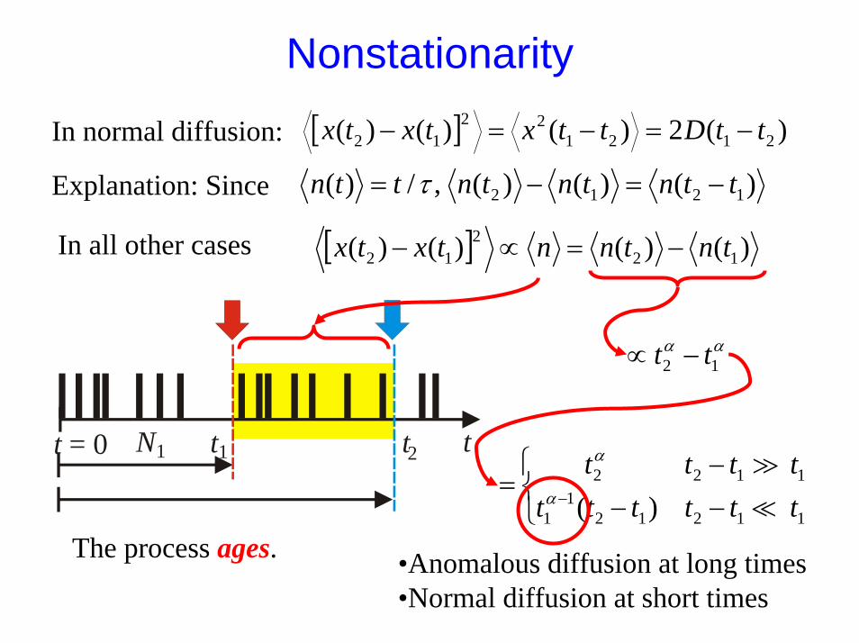
Aging and death of linear response

0 2π 4π 6π 8π 10π t0

m t(

)1

∫=t

tMtdtftm001 )'('sin')( ωµ

iuiuMiuMfum

2)(~)(~

)(~01

ωωµ +−−=

For linear response stagnates:

)(Im)( 01 ωµ iMftm −−→

Trick: + shift theorem in Laplace domain

ieet titi 2/)(sin ωωω −−=

∞→t

I.M. Sokolov and J. Klafter, Phys. Rev. Lett. 97, 140602 (2006)

Exp.: “Experimental quenching of harmonic stimuli …” by P.Allegrini et al.Numerics: M.-C. Néel, A. Zoia and M. Joelson, “Mass transport subject to time-dependent flow with nonuniform sorption in porous media”, PRE 80, 056301 (2009)

We argue that this theory is a universal property, which is not confined to physical processes such as turbulent or excitable media, and that it holds true in all possible conditions, and for all possible systems, including complex networks, thereby establishing a bridge between statistical physics and all thefields of research in complexity.

Kusumi, A., Sako, Y. & Yamamoto, M. Confined lateral diffusion of membranereceptors as studied by single particle tracking (nanovid microscopy). Effects ofCalcium-induced differentiation in cultured epithelial cells. Biophys. J. 65, 2021-2040 (1993).

Kenich, S., Ritchie, K., Kajikawa, E., Fujiwara, T. & Kusumi, A. Rapid hopdiffusion of a G0protein-coupled receptor in the plasma membrane as revealed bysingle-molecule techniques. Biophys. J. 88, 3659-3680 (2005).

Golding, I. & Cox, E.C. Physical nature of bacterial cytoplasm. Phys. Rev. Let.96:098102-1 – 09102-4 (2006).

Seisenberger, G., Ried, M.U. Endreß, T., Büning, H., Hallek, M. & Bräuchle, C.Real-time single-molecule imaging of the infection pathway of an adeno-associated virus. Sience. 294, 1929-1932 (2001)

Single molecule tracking

Ham’s schon mal eins g’sehn?(Have you ever seen one?)

Ernst Mach

•In most experiments on subdiffusion, say in disordered semiconductors, the ensemble average is implied by the multiparticle nature of the problem.

•In single particle tracking experiments moving time average is a typical procedure used to obtain the diffusion coefficient.

Normal diffusion:

Kttx 2)(2 =

[ ]∫−

−+−

=tT

Tdttxttx

tTtx

0

22 ')'()'(1)(

Normal diffusion is an ergodic process: The ensemble average gives the same result as a time-moving average

for a single long trajectory.

•Although the discrimination between normal diffusion and subdiffusion according to

and

seems simple, in practice, however, the situation is quite involved.

αα

αtKtx

)1(2)(2

+Γ=

Kttx 2)(2 =

enstx )(2

•The question of what is the “correct” averaging procedure in the anomalous case has seldom been discussed.

Single particle trajectories calculated from a CTRW with 2/3~)( −ttψ

Model simulations

A. Lubelski, I.M.S, J. Klafter, PRL 100, 250602 (2008)

Ensemble-averaged moving time-averaged behavior

Ensemble-averaged behavior

moving time-averaged behaviorin a single realization

8.1~)( −ttψSome numerical results for the case

The distribution p(K) of diffusion coefficients obtained from time averaged single trajectories for the case of T=2·106, and t=500.

Nonergodicity mimicks inhomogeneity…

8.1~)( −ttψ

Y. He, S. Burov, R. Metzler and E. Barkai, PRL 101, 058101 (2008)A. Lubelski, I.M.Sokolov and J. Klafter, PRL 100, 250602 (2008)

Seisenberger, G., Ried, M.U. Endreß, T., Büning, H., Hallek, M. & Bräuchle, C., Real-time single-molecule imaging of the infection pathway of an adeno-associated virus. Sience. 294, 1929-1932 (2001)

Explanation of the result forens

2 )(T

tx

αAttn ≅ens

)(

[ ] [ ]ens1ens2

2

ens

212 )()()()( tntnatxtx −=−

enstnatx )()( 22 =

•Interchanging the sequence of averaging

[ ] [ ]∫∫ −+=−+=TT

Tdtttt

TAadttnttn

Tatx

0

2

0ensens

2

ens

2 '')'(')'()'(1)( αα

tATatxT

12

ens

2 )( −= αTt <<•For one gets:

•Prediction: time dependent mean diffusion coefficient

2/)( 12eff

−= αATaTK

Numerical check for the prediction

Advice for experimentalists: Check for the time-dependence of diffusion coefficient!

Numerics/ExperimentsAbsence of nonergodicity, and the subdiffusive behavior of the moving time averages is a witness against a whatever trap model of anomalous diffusion.

T.Neusius, I. Daidone, I.M. Sokolov,J.C. Smith, PRL 100, 188103 (2008)

MR121 GSGSW peptide

T.Neusius, I.M. Sokolov, J.C. Smith, PRE 80, 011109 (2009)

The fractal dimension of the main valley in the peptide’s potential landscape is around .7≈fd

)1010( 32 ÷=d

Realistic rugged potential landscapein d = 3.

Universal fluctiuations

I.M. Sokolov, E. Heinsalu, P. Hänggi and I. GoychukUniversal fluctuations in subdiffusive transportEPL 86 (2009) 30009

M. Esposito, K. Lindenberg and I.M. SokolovOn the relation between event-based and time-based current statistics,Europhys. Lett. 89, 10008 (2010)

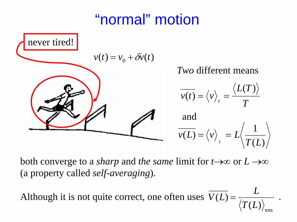
“normal” motion

Two different means

TTL

vtvt

)()( ==

ens)(

)(LTLLV =

)(1)(LT

LvLvL

==

and

both converge to a sharp and the same limit for t→∞ or L →∞(a property called self-averaging).

Although it is not quite correct, one often uses .

)()( 0 tvvtv δ+=never tired!

“anomalous” motion (TOF)

(stolen from Haus and Kehr)

Fixed-time and TOF setups

αψ −−∝ 1)( tt

αttn ∝)(αδ tx ∝

ααδαtxv )1( +Γ=

Units: Time in units of τlength in units of <a>subvelocity in units of

ατα /)1(0 av +Γ=

?Directed RW

Fixed-time velocity

)1()( >>= ntnaxδ

∫−==t

dttttp0

0 ')'(1)(),0( ψχ

∫ −==t

dtttptttp0

1 ')',0()'()(),1( ψχ........................................

∫ −−==t

n dtttnptttnp0

')',1()'()(),( ψχ

no steps up to time t:

1 step up to time t:

n steps up to time t:

[ ] [ ] ( )ααααψψ nuuunuuu

uunp n −≅−≅−

= −− exp)1ln(exp)()(1),( 11

{ } α

αuexLL −=)(ˆ

t = T fixed

⎟⎠⎞

⎜⎝⎛≅ + αααα /1/11

1),(nTL

nTTnp

Universal fluctuations

Scaled velocity 0/ vv=αξ

Distribution of scaled velocity:

⎥⎥⎦

⎤

⎢⎢⎣

⎡⎟⎟⎠

⎞⎜⎜⎝

⎛ +Γ+Γ= +

α

ααα

α

α ξα

αξαξ

/1

/11

/1 )1()1()( Lp

Moments of scaled velocity

1=αξ

)21()1(2 2

2

ααξα +Γ

+Γ=

Moments have to be obtained by additional ensemble averaging!

Independent on T⇒Universal fluctuations

TOF setup

L fixed ⇒ number of steps n fixedNote: meanvelocity cannot be defined as

sincediverges!!! *

t

αtLv /=

)()( /1/1 tnLntp αα

α −−=

Change of variables to ααξ tL /)1( +Γ=

⇓

⎥⎥⎦

⎤

⎢⎢⎣

⎡⎟⎟⎠

⎞⎜⎜⎝

⎛ +Γ+Γ= +

α

ααα

α

α ξα

αξαξ

/1

/11

/1 )1()1()( Lp 1=αξ

)21()1(2 2

2

ααξα +Γ

+Γ=

the same as in the fixed time setup.

Same for periodic potential

FxxVxV −= )2cos()( 0 π

)(Fvv αξ =

Dimensionless velocity is defined as

with

[ ][ ]∫ ∫+

−−

−−= λ λ

αα

β

λβλ

0)()(exp

)]exp(1[)( x

xyUxUdydx

FKFv

as following from the solution of FFPE

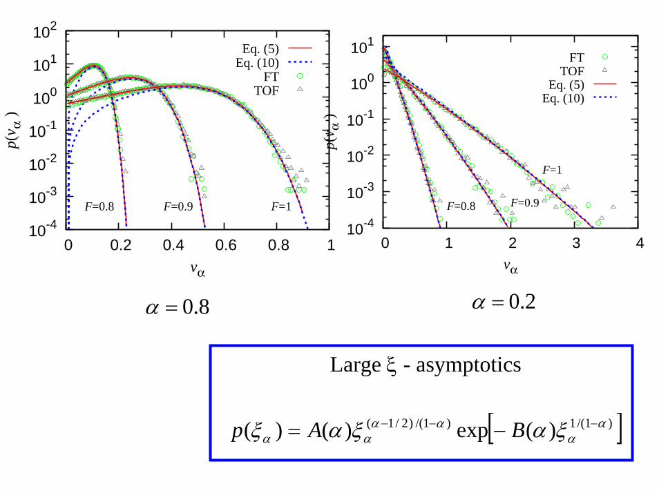
10-4

10-3

10-2

10-1

100

101

0 1 2 3 4

p(v α

)

vα

F=1

F=0.9F=0.8

FTTOF

Eq. (5)Eq. (10)

2.0=α

10-4

10-3

10-2

10-1

100

101

102

0 0.2 0.4 0.6 0.8 1

p(v α

)

vα

F=1F=0.9F=0.8

Eq. (5)Eq. (10)

FTTOF

8.0=α

[ ])1/(1)1/()2/1( )(exp)()( αα

αααα ξαξαξ −−− −= BAp

Large ξ - asymptotics

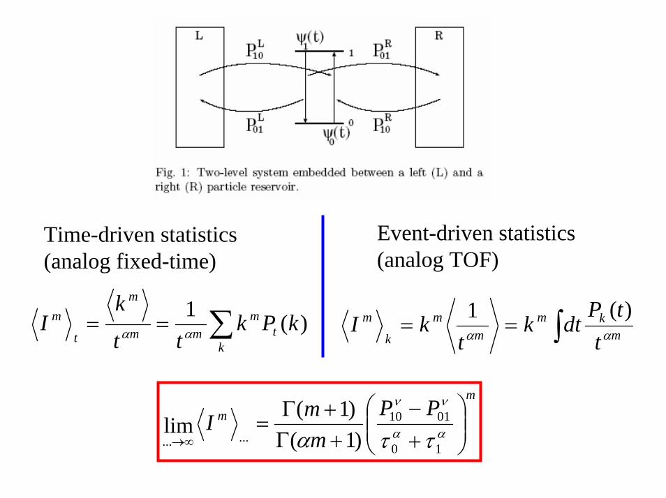
Event-driven statistics (analog TOF)

Time-driven statistics (analog fixed-time)

∑==k

tm

mm

m

t

m kPktt

kI )(1

αα ∫== mkm

mm

k

m

ttP

dtkt

kI αα

)(1

mm PP

mmI ⎟⎟

⎠

⎞⎜⎜⎝

⎛+−

+Γ+Γ

=∞→

αα

νν

ττα 10

0110...... )1(

)1(lim

Conclusions

• Anomalous is normal• Happy families are all alike; every

unhappy family is unhappy in its own way• In subdiffusive systems governed by

CTRW only ensemble averages attain sharp values, the time averages show universal fluctuations!

• If you want to get mean velocity or current, average velocity or current