PHYSICAL REVIEW E 96, 052136 (2017)

Universal Gaussian behavior of driven lattice gases at short times

Valerio Volpati,1 Urna Basu,2 Sergio Caracciolo,3 and Andrea Gambassi21Institut de Physique Théorique (IPhT), Université Paris Saclay, CEA, CNRS, F-91191 Gif-sur-Yvette, France

2SISSA–International School for Advanced Studies and INFN, via Bonomea 265, I-34136 Trieste, Italy3Dipartimento di Fisica and INFN, Università degli Studi di Milano, via Celoria 16, I-20133 Milano, Italy

(Received 24 August 2017; published 27 November 2017)

The dynamic and static critical behaviors of driven and equilibrium lattice gas models are studied in twospatial dimensions. We show that in the short-time regime immediately following a critical quench, the dynamicsof the transverse anisotropic order parameter, its autocorrelation, and Binder cumulant are consistent with theprediction of a Gaussian, i.e., noninteracting, effective theory, both for the nonequilibrium lattice gases and, tosome extent, their equilibrium counterpart. Such a superuniversal behavior is observed only at short times aftera critical quench, while the various models display their distinct behaviors in the stationary states, described bythe corresponding, known universality classes.

DOI: 10.1103/PhysRevE.96.052136

I. INTRODUCTION

The search for universal behavior, which unites a class ofsystems in terms of some common collective properties, liesat the very heart of statistical physics. Both in its static anddynamic manifestations, universality emerges in large systemsof interacting degrees of freedom close to a critical point, whenthey display a behavior that is actually independent of their mi-croscopic features. This critical behavior is usually dictated bysymmetry properties, or conservation laws; critical phenomenaoccurring in various systems having the same symmetriesbelong to the same universality class. Beyond its numerousand celebrated manifestations in equilibrium [1], universalityplays an important role also in the dynamical relaxation ofnonequilibrium systems [2], ranging from diffusive [3] andreaction-diffusion [4] systems to surface growth [5].

Remarkably, universality emerges not only in systems thatare close to their stationary state, but also far from it, i.e., duringthe early stages of the relaxation process, when the correlationlength of the fluctuations of the relevant order parameter isstill very small compared to the system size [6,7]. This factoften translates into the observation of novel critical exponents,but also into the possibility to measure the equilibrium anddynamical critical exponents, which characterize the stationarystate from the observation of this nonequilibrium relaxation,with a substantial reduction of the numerical costs [8–10].

Classifying and characterizing nonequilibrium universalityclasses remain a challenge in statistical physics. Investigationsof lattice models are very useful in this respect: their sim-plicity makes them amenable to numerical, and sometimesanalytical, studies, yet they often show rich and novel physicalphenomena. Lattice gases, which describe stochastic hoppingof particles on a lattice, belong to one such class of models,which has been extensively used to explore critical phenomenain and out of equilibrium [11,12]. These systems oftenshow a continuous transition to an ordered state, where theparticles cluster together, at a certain critical temperature. Suchtransitions are relevant in various physical situations includingbinary mixtures [3], driven diffusive systems [12], viscoelasticfluids [13], vehicular traffic [14], and active matter [15,16].

The critical behavior characterizing the phase transitions inthe various lattice gas models depends on the symmetries oftheir specific dynamics: equilibrium [17], driven [12,18], and

randomly driven [19] lattice gases therefore belong to differentuniversality classes. All these models have one commonfeature though: the density of particles is locally conserved bythe dynamics. Such a conservation law strongly constrains andslows the dynamics down, hence different dynamical behaviorsare expected and observed compared to nonconserved models[2]. While a considerable amount of work has been devotedto study the critical behaviors of the latter, both in and outof equilibrium, much less attention has been given to theshort-time dynamics of the former.

In this paper we show that, remarkably, a sort of superuni-versality, which unites the different lattice gas models, emergesin the short-time regime after a critical quench, irrespectiveof their specific critical behavior. In this regime, in fact,the dynamical behavior of certain observables, which can beconsidered the natural order parameters for these transitionsare described by a noninteracting (Gaussian) effective theory.In particular, we will focus on the behavior of transverseobservables in the driven lattice gas, the randomly drivenlattice gas, and the equilibrium lattice gas in two spatialdimensions. Despite the fact that features such as the drivingor the spatial anisotropy introduce relevant perturbations in thelattice gases, which change entirely the critical properties of thesystem, the short-time behavior of these natural observablesis independent of these features. The peculiar properties ofspecific universality classes are recovered, for all observables,only at longer times.

The paper is organized as follows. In Sec. II we recallthe equilibrium and driven lattice gas models and definecertain relevant observables. A brief discussion of the differenteffective field theories introduced in the past in order to studythe critical behaviors of these models is presented in Sec. III.Based on a Gaussian theory, the dynamical behavior of thetransverse order parameters and autocorrelation of one ofthem are computed. This section elaborates and substantiallyextends the analysis of Ref. [20]. In Sec. IV we comparethe results obtained from Monte Carlo simulations in theshort-time regime with the predictions of a Gaussian effectivetheory for both the driven and equilibrium lattice gases. Thetime evolution of the Binder cumulant starting from variousinitial states is also studied in the various models. Section Vis devoted to the study of the stationary-state behavior of

2470-0045/2017/96(5)/052136(12) 052136-1 ©2017 American Physical Society

VOLPATI, BASU, CARACCIOLO, AND GAMBASSI PHYSICAL REVIEW E 96, 052136 (2017)

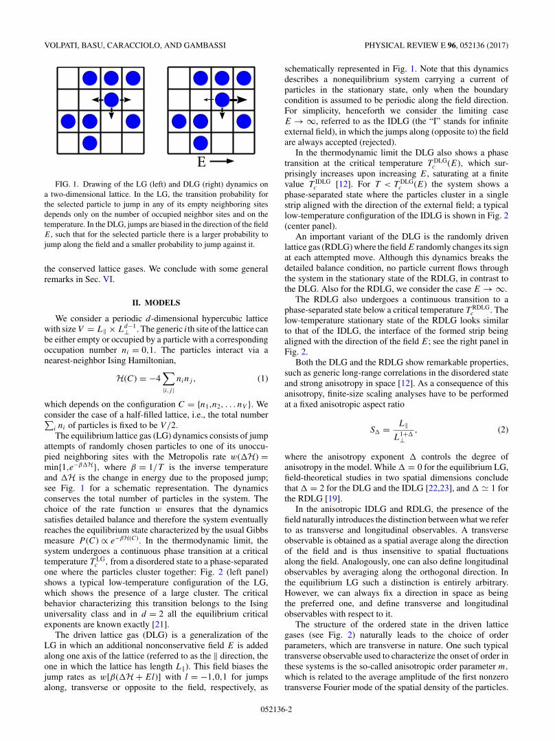
EFIG. 1. Drawing of the LG (left) and DLG (right) dynamics on

a two-dimensional lattice. In the LG, the transition probability forthe selected particle to jump in any of its empty neighboring sitesdepends only on the number of occupied neighbor sites and on thetemperature. In the DLG, jumps are biased in the direction of the fieldE, such that for the selected particle there is a larger probability tojump along the field and a smaller probability to jump against it.

the conserved lattice gases. We conclude with some generalremarks in Sec. VI.

II. MODELS

We consider a periodic d-dimensional hypercubic latticewith size V = L‖ × Ld−1

⊥ . The generic ith site of the lattice canbe either empty or occupied by a particle with a correspondingoccupation number ni = 0,1. The particles interact via anearest-neighbor Ising Hamiltonian,

H(C) = −4∑〈i,j〉

ninj , (1)

which depends on the configuration C = {n1,n2, . . . nV }. Weconsider the case of a half-filled lattice, i.e., the total number∑

i ni of particles is fixed to be V/2.

The equilibrium lattice gas (LG) dynamics consists of jumpattempts of randomly chosen particles to one of its unoccu-pied neighboring sites with the Metropolis rate w(�H) =min{1,e−β�H}, where β = 1/T is the inverse temperatureand �H is the change in energy due to the proposed jump;see Fig. 1 for a schematic representation. The dynamicsconserves the total number of particles in the system. Thechoice of the rate function w ensures that the dynamicssatisfies detailed balance and therefore the system eventuallyreaches the equilibrium state characterized by the usual Gibbsmeasure P (C) ∝ e−βH(C). In the thermodynamic limit, thesystem undergoes a continuous phase transition at a criticaltemperature T LG

c , from a disordered state to a phase-separatedone where the particles cluster together: Fig. 2 (left panel)shows a typical low-temperature configuration of the LG,which shows the presence of a large cluster. The criticalbehavior characterizing this transition belongs to the Isinguniversality class and in d = 2 all the equilibrium criticalexponents are known exactly [21].

The driven lattice gas (DLG) is a generalization of theLG in which an additional nonconservative field E is addedalong one axis of the lattice (referred to as the ‖ direction, theone in which the lattice has length L‖). This field biases thejump rates as w[β(�H + El)] with l = −1,0,1 for jumpsalong, transverse or opposite to the field, respectively, as

schematically represented in Fig. 1. Note that this dynamicsdescribes a nonequilibrium system carrying a current ofparticles in the stationary state, only when the boundarycondition is assumed to be periodic along the field direction.For simplicity, henceforth we consider the limiting caseE → ∞, referred to as the IDLG (the “I” stands for infiniteexternal field), in which the jumps along (opposite to) the fieldare always accepted (rejected).

In the thermodynamic limit the DLG also shows a phasetransition at the critical temperature T DLG

c (E), which sur-prisingly increases upon increasing E, saturating at a finitevalue T IDLG

c [12]. For T < T DLGc (E) the system shows a

phase-separated state where the particles cluster in a singlestrip aligned with the direction of the external field; a typicallow-temperature configuration of the IDLG is shown in Fig. 2(center panel).

An important variant of the DLG is the randomly drivenlattice gas (RDLG) where the field E randomly changes its signat each attempted move. Although this dynamics breaks thedetailed balance condition, no particle current flows throughthe system in the stationary state of the RDLG, in contrast tothe DLG. Also for the RDLG, we consider the case E → ∞.

The RDLG also undergoes a continuous transition to aphase-separated state below a critical temperature T RDLG

c . Thelow-temperature stationary state of the RDLG looks similarto that of the IDLG, the interface of the formed strip beingaligned with the direction of the field E; see the right panel inFig. 2.

Both the DLG and the RDLG show remarkable properties,such as generic long-range correlations in the disordered stateand strong anisotropy in space [12]. As a consequence of thisanisotropy, finite-size scaling analyses have to be performedat a fixed anisotropic aspect ratio

S� = L‖L1+�

⊥, (2)

where the anisotropy exponent � controls the degree ofanisotropy in the model. While � = 0 for the equilibrium LG,field-theoretical studies in two spatial dimensions concludethat � = 2 for the DLG and the IDLG [22,23], and � 1 forthe RDLG [19].

In the anisotropic IDLG and RDLG, the presence of thefield naturally introduces the distinction between what we referto as transverse and longitudinal observables. A transverseobservable is obtained as a spatial average along the directionof the field and is thus insensitive to spatial fluctuationsalong the field. Analogously, one can also define longitudinalobservables by averaging along the orthogonal direction. Inthe equilibrium LG such a distinction is entirely arbitrary.However, we can always fix a direction in space as beingthe preferred one, and define transverse and longitudinalobservables with respect to it.

The structure of the ordered state in the driven latticegases (see Fig. 2) naturally leads to the choice of orderparameters, which are transverse in nature. One such typicaltransverse observable used to characterize the onset of order inthese systems is the so-called anisotropic order parameter m,

which is related to the average amplitude of the first nonzerotransverse Fourier mode of the spatial density of the particles.

052136-2

UNIVERSAL GAUSSIAN BEHAVIOR OF DRIVEN LATTICE . . . PHYSICAL REVIEW E 96, 052136 (2017)

FIG. 2. Snapshots of the typical low-temperature (ordered) configurations of the LG (left), IDLG (center), and RDLG (right) at half-fillingand in the stationary state as obtained from the Monte Carlo simulation on square lattices of size 128 × 128. Blue dots represent particles, whileempty sites are shown as gray dots. In the case of the LG on a square lattice, the interface between the high-density and low-density regionscan be aligned with either axis of the lattice with equal probability; here we report an instance in which it is aligned with the vertical direction.In the driven cases, both for the IDLG and the RDLG, the driving occurs here along the horizontal direction and the interface between thehigh-density and low-density regions is parallel to the driving direction. The temperature T = 2.0 is below the critical temperature in all thethree cases.

To define it precisely, let us consider a (d = 2)-dimensionallattice of size V = L‖ × L⊥ and associate, to each site (x,y),a spin variable σxy = 2nxy − 1, which takes values ±1. Therelevant quantity is its Fourier transform

σ̃ (k‖,k⊥) =L‖−1∑x=0

L⊥−1∑y=0

ei(k‖x+k⊥y)σxy, (3)

where, due to the periodic boundary conditions, the allowedlongitudinal and transverse momenta are

(k‖,k⊥) =(

2πn‖L‖

,2πn⊥L⊥

), (4)

with integers 0 � n‖ � L‖ and 0 � n⊥ � L⊥. The half-fillingcondition on particle density implies that the total magnetiza-tion

∑xy σxy vanishes and in turn, σ̃ (0,0) = 0.

The anisotropic order parameter m is defined as thestatistical average of the absolute value of the first nonzerotransverse mode μ = σ̃ (0,2π/L⊥), i.e., as

m = 〈|μ|〉/V, (5)

where 〈·〉 denotes the statistical average. In order to character-ize the dynamical behavior it is also instructive to consider thetemporal autocorrelation function Cm of the anisotropic orderparameter, i.e.,

Cm(s,t) = 1

V[〈|μ(s)μ(t)|〉 − 〈|μ(s)|〉〈|μ(t)|〉]. (6)

An alternative observable used to detect the onset of an orderedphase in these systems is the average absolute value O of themagnetization along the field direction, which was proposedand studied in Ref. [9],

O = 1

V

L⊥−1∑y=0

˝∣∣∣∣∣∣L||−1∑x=0

σxy

∣∣∣∣∣∣˛. (7)

Both O and m are expected to be nonzero in the orderedphase, where the particles cluster together to form a singlestrip aligned along the direction of the drive, although theirstationary values are expected to be different. On the otherhand, both m and O vanish in the disordered phase in the

thermodynamic limit thus providing two alternative definitionsof an order parameter.

The alternative order parameter O is also a transverseobservable, as it can be expressed as a sum of transverse modes,

O = 1

V 2

L⊥−1∑y=0

˝∣∣∣∣∣∣L‖−1∑x=0

∑k‖,k⊥

e−i(k‖x+k⊥y)σ̃ (k‖,k⊥)

∣∣∣∣∣∣˛

= 1

V

⟨∣∣∣∣∣L⊥−1∑n⊥=1

σ̃

(0,

2πn⊥L⊥

)∣∣∣∣∣⟩

. (8)

The last equality follows from the condition σ̃ (0,0) = 0 andthe fact that the expectation value on the first line does notdepend on y.

The critical behavior of the three lattice gas modelsmentioned above belongs to three distinct universality classes.In Sec. III below we will briefly mention the differenteffective field theories, which describe the critical behaviorsof these models. Next, we will discuss an effective Gaussian(noninteracting) theory and some aspects of the behavior ofall the conserved lattice gases, which turn out to be describedby it [20].

III. MESOSCOPIC DESCRIPTION:FIELD-THEORETICAL APPROACH

The critical behavior of the lattice gas models can beunderstood based on effective, mesoscopic field-theoretical de-scriptions of their dynamics [2]. Near criticality, the evolutionof the coarse-grained local spin density φ(x,t) is expected tobe governed by a Langevin equation, which takes into accountthe relevant interactions specific to each universality class.We briefly recall some basic facts about the effective theoriescorresponding to the lattice gases discussed here.

Equilibrium lattice gas. The phase transition in the equilib-rium lattice gas belongs to the Ising universality class, whichis characterized by the standard φ4 theory [17]. Its dynamics,in the case of conserved order parameter φ, is described by thecorresponding Langevin equation (known as Model B) [2,3],

∂tφ = α[(τ − ∇2)∇2φ] + u∇2φ3 − ∇ · ξ, (9)

052136-3

VOLPATI, BASU, CARACCIOLO, AND GAMBASSI PHYSICAL REVIEW E 96, 052136 (2017)

where τ measures the distance from the critical point, u > 0 isthe interaction strength, α is a positive constant, and ξ is a whitenoise with 〈ξi(x,t)ξj (x ′,t ′)〉 ∝ δij δ

d (x − x ′)δ(t − t ′). The re-sulting critical behavior and exponents are known exactly ind = 2 [21] while the upper critical spatial dimensionality dc

is 4.Driven lattice gas. The mesoscopic description of the

driven lattice gas was developed independently by Janssenand Schmittmann [22] and Leung and Cardy [23]. This theory,henceforth referred to as JSLC theory, differs from the LG intwo respects: the external field introduces a new interactionterm and induces strong anisotropy. Correspondingly, theLangevin equation describing the evolution of the coarse-grained spin density in the near-critical DLG (and IDLG) isgiven by

∂tφ = α[(τ − ∇2⊥)∇2

⊥φ + τ‖∇2‖φ + E∇‖φ2]

+u∇2⊥φ3 − ∇ · ξ, (10)

where E represents the coarse-grained driving field, while ∇⊥and ∇‖ denote spatial derivatives orthogonal and parallel to thedriving directions, respectively. The presence of an additionalrelevant interaction term E∇‖φ2 and spatial anisotropy causethe critical behavior to change compared to that of the Isinguniversality class. Also in this case, the critical exponentsare known exactly in all spatial dimensions d � 2 up to theupper critical dimension dc = 5; of primary importance forthe purpose of the present study is the anisotropy exponent� = 2 in two spatial dimensions, which will intervene in thefollowing analysis. The specific form of the interaction termcauses the behavior of φ at vanishing parallel wave vectork‖ = 0 to be effectively described by a noninteracting theoryand therefore its transverse fluctuations are expected to bedescribed by a simple Gaussian theory discussed below [24].

Randomly driven lattice gas. The Langevin equation takesa different form compared to Eq. (10) when the driving fieldchanges sign randomly, i.e., in the case of the RDLG; theparticle current is no longer relevant, but anisotropy continuesto be a significant factor, resulting in the effective equation

∂tφ = α[(τ − ∇2⊥)∇2

⊥φ + τ‖∇2‖φ] + u∇2

⊥φ3 − ∇ · ξ. (11)

In turn, this results in yet another universality class, differentfrom both LG and DLG; the critical exponents are known interms of a series expansion around the upper critical dimensiondc = 3 [19,25]. In addition, the anisotropy exponent � 1differs from that of the DLG in d = 2.

Gaussian effective theory. The Gaussian or noninteractingtheory describes a fluctuating field in the absence of nonlinearinteractions. The corresponding Langevin equation for asystem with locally conserved field can be obtained by settingu = 0 in Eq. (9),

∂tφ = α(τ − ∇2)∇2φ − ∇ · ξ. (12)

Irrespective of the fact that the phase transitions in the threedifferent models, namely LG, DLG, and RDLG belong tothree different universality classes, the short-time dynamicalbehaviors of certain transverse observables, after a quench tothe critical point, turn out to be very similar in all these models.In fact, as discussed in Ref. [20], transverse modes in all thelattice gas models show a behavior at short times, which is

consistent with a free theory, i.e., the distribution of transversemodes is effectively Gaussian. Some of the results of thissection have already been briefly anticipated in Ref. [20]; in thefollowing we also provide additional details of that analysis.

In particular, our objective is to determine the temporalbehavior of the order parameters introduced in Sec. II fora model system, which is described by an effective Gaussiantheory. In order to do so we need to look at the time evolution ofthe transverse modes σ̃k [defined in Eq. (3)], which is obtainedby taking the Fourier transform of the Langevin equation (12).However, since we are interested in lattice models, the spatialgradients in that equation have to be interpreted as beingdefined on a lattice. Consequently, the amplitude σ̃k of thetransverse mode k = (0,k⊥) evolves according to,

d

dtσ̃k(t) = −γkσ̃k(t) + ik̂ η̃k(t), (13)

where k̂ = 2 sin(k/2) is the lattice momentum and

γk = α(τ + k̂2)k̂2. (14)

As mentioned above, α is a coarse-grained diffusion constant,possibly depending on the lattice parameters and τ measuresthe distance from the critical point. Additionally, η̃ is a whitenoise in momentum space, obtained by taking the Fouriertransform of the noise in real space, and is also δ correlated,with

〈η̃k(t)η̃k′(t ′)〉 = 2αTηL‖L⊥δ(k + k′)δ(t − t ′), (15)

where the normalization factor Tη signifies an effectivetemperature associated with the noise in terms of which thefluctuation-dissipation theorem [26] is effectively satisfiedwhen looking at correlations and response functions ofthe transverse fluctuations. Note that the noise strength inmomentum space is proportional to the volume of the latticebecause of the discrete nature of the allowed momenta.

Let us consider the case in which the system is initially in adisordered configuration corresponding to a high temperature,so that σ̃k(t = 0) = 0 for all transverse modes k. For this initialcondition Eq. (13) has the solution

σ̃k(t) = ik̂

∫ t

0dsηk(s)e−γk(t−s). (16)

This leads to a Gaussian behavior, i.e., the kth Fourier modehas a Gaussian probability distribution P at any time t,

P [σ̃k(t)] = Nk(t) exp

[− |σ̃k(t)|2

L‖L⊥G⊥(t,k)

], (17)

where G⊥(t,k) is the transverse propagator,

G⊥(t,k) = 1

L‖L⊥〈|σ̃k(t)|2〉 (18)

and Nk(t) = [πL‖L⊥G̃⊥(t,k)]−1 is the normalization. Thetransverse propagator is easily computed from Eq. (16),

G⊥(t,k) = αTη

k̂2

γk

(1 − e−2γkt ). (19)

052136-4

UNIVERSAL GAUSSIAN BEHAVIOR OF DRIVEN LATTICE . . . PHYSICAL REVIEW E 96, 052136 (2017)

The anisotropic order parameter m(t) [defined in Eq. (5)] canbe calculated easily from Eqs. (19) and (17),

m(t) = 2πNk1 (t)

L‖L⊥

∫ ∞

0drr2 exp

[− r2

L‖L⊥G⊥(t,k1)

]

=√

π

4

G⊥(t,k1)

L‖L⊥, (20)

where k1 ≡ 2π/L⊥ indicates the first nonzero mode allowedin the transverse direction.

We are particularly interested in the dynamical behavior ofm(t) in the short-time regime, i.e., immediately after the criticalquench, when the system is far from reaching its stationarystate. In this regime, one can expand the exponential in Eq. (19)and keep only the linear term in t, finding, for any τ,

G⊥(t,k1) = 2αTηk̂21 t + O(t2). (21)

In the thermodynamic limit, i.e., for large L⊥, we have k̂1 =2 sin(k1/2) 2π/L⊥. To the leading order in t, then, Eq. (20)implies,

m(t) ≈√

2π3αTη

t

L‖L3⊥

, (22)

for t � L4⊥. This spells a clearer meaning to the term short-

time regime: this behavior is expected to hold up to a time thatis much shorter than the time scale set by the system size.

At longer times, instead, m(t) approaches a stationary valuemS , which can also be obtained from Eq. (20). In particular, atthe critical point τ = 0,

mS ≡ limt→∞ m(t) =

√Tη

16π

L⊥L‖

, (23)

which depends only on the isotropic aspect ratio L⊥/L‖.In order to predict the behavior of the order parameter

O, defined in Eq. (8), we first note that as each singlemode σ̃k [see Eq. (13)] is a stochastic variable with aGaussian distribution, their sum in Eq. (8) also has a Gaussiandistribution. Accordingly,

O(t) =√

π

4

D(t)

L⊥L||, (24)

where D(t) is the sum of the transverse propagators of themodes appearing in Eq. (8), i.e.,

D(t) =L⊥−1∑n⊥=1

G⊥

(t,

2πn⊥L⊥

). (25)

For sufficiently large L⊥ one can take the continuum limitof this expression and the sum over n⊥ is replaced by amomentum integral; at the critical point τ = 0, one then finds,

D(t) TηL⊥∫ π

−π

dk

2π

1 − e−2αtk4

k2

= TηL⊥π2

{(2αt)1/4π [�(3/4) − �(3/4,2αtπ4)]

+ e−2αtπ4 − 1}, (26)

where �(x) is the Gamma function and �(x,s) is the incom-plete Gamma function; see, e.g., Eq. 8.2.2 in Ref. [27]. Inparticular, for large enough αt � 1,

D(t) TηL⊥π

�(3/4)(2αt)1/4. (27)

Accordingly, from Eq. (25), O grows, in this intermediate timeregime, as

O(t) t1/8

2L1/2‖

√Tη(2α)1/4�(3/4), (28)

i.e., O(t) ∼ t1/8 upon increasing t. We emphasize here thatthe limits L⊥ → ∞ and t → ∞ do not commute. To obtainthe stationary value OS of O(t), one can perform a directsummation in Eq. (25) with G⊥ given by Eq. (19), and get,

limt→∞ D(t) = Tη

L⊥−1∑n⊥=1

1

2 sin(πn⊥/L⊥)= Tη

12(L2

⊥ − 1).

Accordingly, from Eq. (25), assuming L⊥ � 1,

OS ≡ limt→∞ O(t) =

√Tηπ

48

L⊥L‖

. (29)

One comment is in order here. As we will show in the nextsection, the short-time behavior of the order parameters m andO predicted on the basis of the effective Gaussian theory [inEqs. (22) and (28)] holds in driven lattices gases irrespectiveof the system size and of any specific geometrical aspect ratioof the lattices [20]. On the other hand, the stationary state,reached at larger times, is different for the various lattice gasesand it is only for the specific case of IDLG that the JSLCtheory predicts a Gaussian behavior of transverse modes, alsoin the stationary state. Consequently, the behaviors of m andO, in the stationary state, as predicted by the Gaussian theory[in Eqs. (23) and (29), respectively] are expected to hold onlyfor the IDLG assuming the appropriate anisotropic scaling.

The auto-correlation Cm of the order parameter m, definedin Eq. (6), can also be easily calculated within the Gaussianmodel discussed here. The joint distribution of σ̃k(s) and σ̃k(t)following from Eq. (16) is nothing but a multivariate Gaussiandistribution [28],

P [σ̃k(s), σ̃k(t)] = 1

4π2D exp

{− 1

2D [λtt |σ̃k(s)|2

+ λss |σ̃k(t)|2 − 2λstRe (σ̃k(s)σ̃ ∗k (t))]

},

(30)

where ∗ denotes the complex conjugate, and

λt1t2 = 〈[Reσ̃k(t1)][Reσ̃k(t2)]〉

= αTηV

2

k̂2

γk

e−γk (t2−t1)(1 − e−2γkt1 ), (31)

with D = λssλtt − λ2st > 0. To obtain the autocorrelation

Cm(s,t) of the lowest mode μ with k = k1, we need to compute

052136-5

VOLPATI, BASU, CARACCIOLO, AND GAMBASSI PHYSICAL REVIEW E 96, 052136 (2017)

a double spherical integral,

〈|μ(s)μ(t)|〉 = 1

4π2D

∫ ∞

0dr1dr2

∫ 2π

0dθ1dθ2r

21 r2

2

× exp

{− 1

2D[λtt r

21 + λssr

22 − 2λst r1r2

× cos(θ2 − θ1)]}

=√

λttλss[2E(y) − (1 − y)K(y)], (32)

where y = λ2st /(λttλss). Here K(x) and E(x) are the Legen-

dre’s complete elliptic integrals of the first and second kind,respectively; see Sec. 19.2 in Ref. [27].

In the short-time regime where s < t � γ −1k , one has

λssλtt (αTηV )2k̂4st and λ2st /(λttλss) s/t. The connected

correlation function [defined in Eq. (6)], in this regime, is thenobtained from Eq. (32) and Eq. (20),

Cm(s,t) = αTηk̂2t

√s

t

[2E

(s

t

)−

(1 − s

t

)K

(s

t

)− π

2

].

(33)

Moreover, for small x,

K(x) = π

2+ πx

8+ O(x2),

E(x) = π

2− πx

8+ O(x2). (34)

Combining Eq. (33) with Eq. (34) yields, to the leading orderin s/t ,

Cm(s,t) = αTηk̂2 π

8t

(s

t

)3/2

. (35)

This behavior is expected to hold in the short-time regime, i.e.,for s/t � 1.

A useful indicator of deviation from the Gaussian behavioris the so-called Binder cumulant g [29]. Its appropriatedefinition for systems with conserved order parameter has beenproposed in Ref. [30],

g = 2 − 〈|μ|4〉〈|μ|2〉2

, (36)

where μ is defined before Eq. (5). For a Gaussian field,〈|μ|4〉 = 2〈|μ|2〉2 = 2V 2G2

⊥ and thus the Binder cumulantvanishes. Its possible finite value is therefore a good measureof the deviation from a Gaussian behavior.

In the following Secs. IV and V we compare the predic-tions of the Gaussian theory with the results of numericalsimulations in the three different lattice gas models, both inthe short-time regime and in the stationary state.

IV. SHORT-TIME REGIME

We perform Monte Carlo simulations to determine thedynamical behavior of the order parameters m and O and theirautocorrelations in all the three lattice gas models introducedabove, namely, LG, IDLG, and RDLG. The simulations aredone on two-dimensional rectangular lattices of size L‖ × L⊥where ‖ and ⊥ denote the directions parallel and transverse to

the driving field in IDLG and RDLG, and arbitrary directionsin LG. Periodic boundary conditions are assumed in both thespatial directions. Each Monte Carlo step, which sets the unitof time, consists of V = L‖L⊥ attempted jumps.

In each case, the system is prepared initially in a disorderedconfiguration corresponding to the stationary state at T → ∞in which both the order parameters m and O vanish. The timeevolution is studied at the critical temperature Tc, which isdifferent for the three models with T LG

c = 2.269 [21], T IDLGc =

3.20 [10], and T RDLGc = 3.15 [20], (see also Sec. V B below

for the determination of T RDLGc ), respectively. In Sec. IV C

below we will also consider the time evolution of the Bindercumulant starting from different initial conditions and studyhow this affects the short-time Gaussian behavior.

A. Evolution of the order parameters

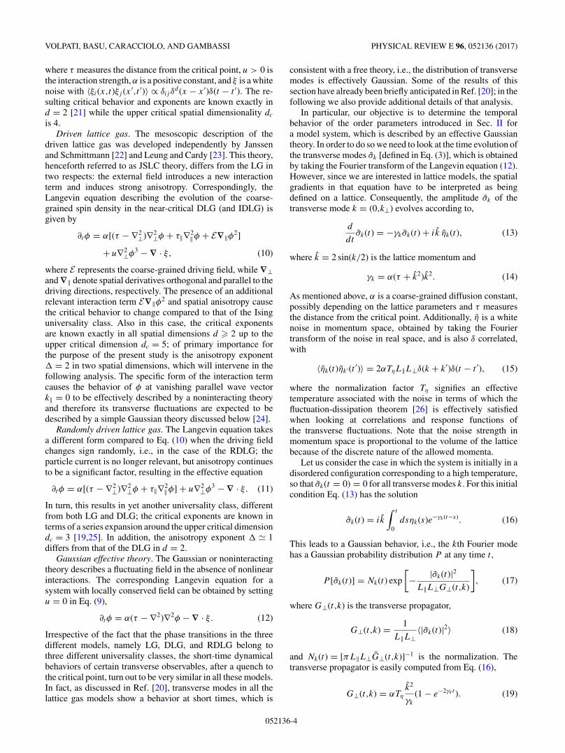
The behavior of the order parameters m and O agree verywell with the predictions of the Gaussian theory in Eqs. (22)and (28), the only exception being the case of O in LG [20].This can be seen in Fig. 3 where we compare m(t) and O(t)for different models for the same system size. In the short-timeregime the curves corresponding to IDLG and RDLG arealmost identical with m(t) ∼ t1/2 and O(t) ∼ t1/8. For LG, in-stead, O(t) ∼ t1/10 while the anisotropic order parameter m(t)still shows a ∼t1/2 growth, consistent with a Gaussian behav-ior. The different behavior of O in LG can be attributed to thefact that the higher modes show deviation from Gaussian be-havior in this case (see Ref. [20] for more details). This obser-vation is the first indication that the Gaussian behavior is moreapparent in the driven models than in the equilibrium one.

The Gaussian theory provides a way to determine thenormalization constants α and Tη independently. From a fitof the curves of m(t) and O(t) according to Eqs. (22) and (28)in the short-time regime (excluding possible lattice effects forvery small t) one can determine the combinations αTη andα1/4Tη, respectively. These values along with the individualestimates of α and Tη obtained using them are reported inTable II. The values of α and Tη for the IDLG and the RDLG arevery close, consistent with their behavior as seen in Fig. 3. Wehave also checked that these values do not depend significantly

100 102 104t10-3

10-2

10-1

m

IDLGRDLGLG

100 102 104t

10-1O

IDLGRDLGLG

(a) (b)

t1/8

t1/10

t1/2

t1/2

FIG. 3. Short-time dynamical behavior of the order parametersm (a) and O (b) at T = Tc in all the lattice gas models: RDLG(topmost curves in both panels), IDLG (middle curves), and LG(lowest curves), on a L‖ × L⊥ = 128 × 32 lattice. The anisotropicorder parameter m grows as t1/2 as a function of time t in all casesin (a). In (b), O grows as t1/8 upon increasing t both for the IDLGand the RDLG, while it grows as t1/10 for the equilibrium LG. Eachcurve has been obtained by averaging over at least 104 independentrealizations.

052136-6

UNIVERSAL GAUSSIAN BEHAVIOR OF DRIVEN LATTICE . . . PHYSICAL REVIEW E 96, 052136 (2017)

10-2 10-1 100s/t

10-4

10-2

Cm

(s,t)tζ

s=50s=100s=150s=200

102 103t

10-1

100

Cm

(s,t)

(a)

IDLG

10-2 10-1 100s/t

10-4

10-2

Cm

(s,t)tζ

s=50s=100s=150s=200

102 103t

10-1

100

Cm

(s,t)

(b)

RDLG

10-2 10-1 100s/t

10-4

10-2

Cm

(s,t)t-ζ

s=100s=150s=200s=250

102 103t

10-1

100

Cm

(s,t)

(c)

LG

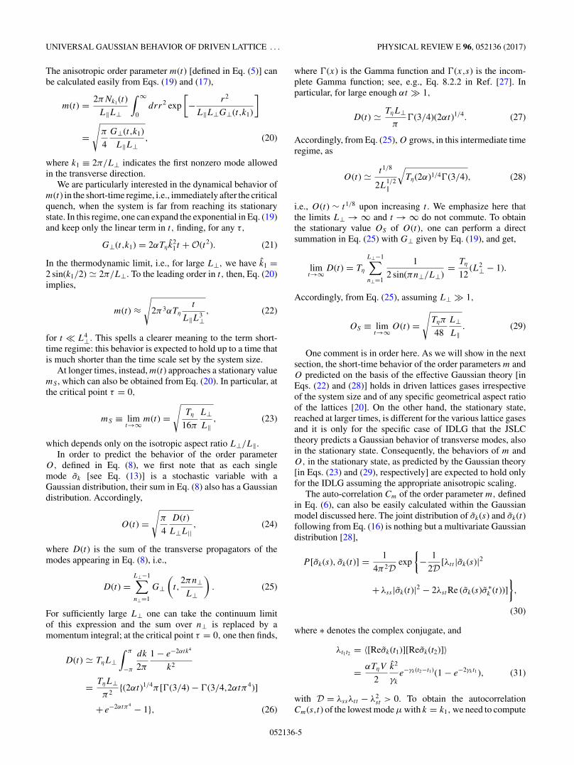
FIG. 4. Plot of Cm(t,s)t−ζ as a function of s/t for (a) IDLG, (b) RDLG, and (c) LG and a set of values of s. The best collapse of the curvesis attained with ζ = 0.96(2) for IDLG, ζ = 0.96(2) for RDLG and ζ = 0.95(1) for LG. The dashed red lines correspond to (s/t)3/2 and theinsets show the unscaled data in all three cases. The dash-dotted line in (c) shows the behavior (s/t)3/2(1 − 0.19 log(s/t)). The system size isL‖×L⊥ = 128 × 32 in all panels. Each curve has been obtained by averaging over 105 independent realizations.

on the system size. For the LG, instead, only m follows theGaussian prediction and we can determine the combinationαTη only, not the individual parameters and this estimate ofαTη (see lowest row on Table II) differs considerably fromthose for the driven lattice gases.

It is interesting to note that Tη/Tc is very close to unityfor both IDLG and RDLG. This suggests that the dynamicsof the lowest transverse modes at short-times is not only ruledby an effective Gaussian model leading to a linear Langevinequation, but also that this dynamics occurs as in an equilib-rium system at the same temperature as that ruling the particletransitions on the lattice transversely to the driving field.

B. Autocorrelation of the order parameter

Close to a phase transition, the temporal autocorrelation ofthe order parameter also typically carries the signature of theuniversal critical behavior [31]. This fact has been used in theliterature to distinguish between different universality classesof driven lattice gases by studying, e.g., the particle densityautocorrelation of the IDLG [10]. In this view, it is interestingto explore the behavior of the autocorrelation of the anisotropicorder parameter m for the various lattice gas models andcompare it with the prediction of the Gaussian theory.

To this end, we measure the autocorrelation Cm(s,t)[defined in Eq. (6)] of the order parameter m in the short-timeregime after a critical quench for all the three models usingMonte Carlo simulations. Figure 4 shows plots of Cm(s,t)t−ζ

as a function of s/t for IDLG [Fig. 4(a)], RDLG [Fig. 4(b)],and LG [Fig. 4(c)] where ζ is the exponent obtained from thebest collapse of the data. In particular, we obtain, ζ = 0.96(2)for the IDLG, ζ = 0.96(2) for the RDLG and ζ = 0.95(2)for the LG. All these three values agree rather well withthe prediction ζ = 1 of the Gaussian theory, see Eq. (35).Moreover, the behaviors of the scaled curves is also consistentwith the Gaussian theory in all the cases, showing a growth∼ (s/t)3/2 upon increasing s/t (dashed red lines in Fig. 4).Note that, in the LG case the (s/t)3/2 behavior is seen for anarrower window with s/t � 1 compared to the driven cases;this, again, seemingly suggest that LG is, in some sense, lessGaussian than its driven counterparts. This is confirmed by thefact that a better fit is obtained by introducing a logarithmicviolation to the (s/t)3/2 behavior. In Fig. 4(c) the dash-dotted

line shows a curve of the form (s/t)3/2[1 − b log(s/t)] forcomparison.

It must be mentioned here that other two-time quantitiessuch as the density autocorrelation, which cannot be expressedas a function of the transverse modes only, can be successfullyused in order to discriminate the different models evenin the short-time regime, as it has been demonstrated inRef. [10]. This fact clearly shows that, in the presence of alocal conservation law, an attentive choice of observables isnecessary in order to be able to distinguish between differentuniversality classes and that some choices turn out to beinadequate at short times in spite of the fact that they naturallyappear as being bona fide order parameters.

C. Binder cumulant: Dependence on the initial condition

The Binder cumulant g is an effective measure of Gaussianbehavior or deviation therefrom. Beyond its widespreadapplications in equilibrium statistical physics, it has also beenused in the context of nonequilibrium lattice gases in orderto characterize the stationary-state behavior [25,30]. Morerecently, g has been used to show that the dynamical behaviorof the first nontrivial transverse mode is well described by aGaussian theory up to a time which scales as Lz

⊥ in all the threedifferent lattice gas models [20]. However, the stationary valueof the Binder cumulant conclusively distinguishes betweenthese three universality classes. It is therefore natural to askwhat is the origin of the observed superuniversal Gaussianbehavior in the short-time regime and, via the analysis of thebehavior of g, to investigate how much of it depends on thespecific choice of the initial condition, chosen to be disorderedin Ref. [20]. Accordingly, in the following we explore thedynamical behavior of the Binder cumulant starting from thevarious initial conditions depicted schematically in Fig. 5. Inparticular, we consider the following configurations:

(I) Disordered configuration: This corresponds to a typicalconfiguration at high temperature, as the particles are dis-tributed randomly; we ensure that the magnetization on eachrow is exactly zero so that m vanishes in this state. This initialcondition is the one used to study the behavior of the orderparameters in Sec. IV.

(II) Column-ordered configuration: This initial condi-tion resembles a phase-separated state but the interface is

052136-7

VOLPATI, BASU, CARACCIOLO, AND GAMBASSI PHYSICAL REVIEW E 96, 052136 (2017)

I II

III IV

FIG. 5. Schematic representations of the various initial conditionsconsidered in Sec. IV C. The blue dots correspond to particles. In thedriven systems the field acts along the horizontal direction.

orthogonal to the direction of the field and hence theanisotropic order parameter m vanishes. Note that this con-figuration corresponds to one of the two equivalent low-temperature configurations of the LG on a square lattice.

(III) Mixed-ordered configuration: For this initial condi-tion the particles are arranged on the lattice in order toform a checker board pattern, the top right and bottom leftsubrectangles are the only ones being occupied. Also in thisconfiguration the order parameter m vanishes.

(IV) Row-ordered configuration: Here we start from thephase-separated state, with the interface being parallel to thedirection of the drive. In the case of the LG, this is taken tobe the x direction, mimicking the ordered configuration in thedriven cases. This configuration corresponds to a finite nonzerovalue of m.

The Binder cumulant g is computed, as discussed in Sec. III,with reference to the first transverse mode, according toEq. (36).

Figure 6 shows plots of the time evolution of the Bindercumulant g starting from these various initial configurationsfor all the three lattice gas models, at the corresponding criticaltemperatures. Although the three initial conditions I, II, and IIIall correspond to a vanishing value of the order parameter m,

the particle distributions in space are very different in the threecases. However, in each case, after an initial transient there isan intermediate regime where the transverse fluctuations areGaussian, as indicated by the vanishingly small value of g (seethe light orange, dark green, and purple curves in Fig. 6). Thisobservation reinforces the idea that, at criticality, the short-timeevolution of the transverse modes of the lattice gases is indeedgoverned by a Gaussian dynamics as in Eq. (16) as long asthe initial configuration of the lattice is a not-ordered one, i.e.,with a vanishing initial value of the order parameter.

Note that, the LG, in contrast with the IDLG and the RDLG,shows a more pronounced initial nonzero stretch. Also, forthe LG with the column initial condition II, the onset ofgrowth of the Binder cumulant is marked by an unexpecteddip. These features speak for the Gaussian behavior being lesspronounced in LG compared to the driven lattice gases.

In fact, it is rather surprising that the Binder cumulant showsa vanishingly small value for a considerably long time forthe LG [see Fig. 6(c)], because, as it is well known, it isactually described by an interacting φ4 theory characterizedby a nonvanishing stationary value of the cumulant g [17].

In order to understand the short-time behavior of the Bindercumulant in the LG model we perform a perturbative analysisfor the φ4 theory around the Gaussian fixed point. We calculatethe evolution of g for a small interaction strength u, as definedin Eq. (9). It turns out that the growth of g is slowed down by afactor of k4 compared to the nonconserved case. Consequently,for the first transverse mode with the smallest value of k, g

appears to be vanishingly small; see Appendix A for the details.The configuration IV corresponds to an ordered state, and

in this case, for all the models considered, the Binder cumulantg starts from unity and monotonically decreases towards thestationary value (uppermost, light brown curves in the plotsof Fig. 6). In the long-time limit, as expected, g attains the

100 101 102 103 104t

-0.4

0

0.4

0.8

g

IIIIIIIV

(a)

IDLG

100 101 102 103 104t

-0.4

0

0.4

0.8

g

IIIIIIIV

(b)

RDLG

100 102 104t

-0.4

0

0.4

0.8

g

IIIIIIIV

(c)

LG

FIG. 6. Time evolution of the Binder cumulant g for (a) IDLG, (b) RDLG, and (c) LG and the various initial conditions indicated by I, II,III, and IV in Fig. 5. The numerical data have been obtained from Monte Carlo simulations on a lattice of size L‖ × L⊥ = 32×32 in all thecases. The curves for IDLG and RDLG are obtained by averaging over at least 104 and 105 independent realizations, respectively. For the LG,instead, at least 105 independent realizations have been used to obtain the curves corresponding to initial conditions II and III whereas thosefor the initial conditions I and IV are generated by using 5×103 realizations.

052136-8

UNIVERSAL GAUSSIAN BEHAVIOR OF DRIVEN LATTICE . . . PHYSICAL REVIEW E 96, 052136 (2017)

same stationary value irrespective of the initial conditions,depending only on the specific model. This is clearly shownby all curves in Fig. 6.

V. STATIONARY STATE

The stationary state of the lattice gas models bears thesignatures of the specific universality class, displaying differ-ent behavior for the three different models considered in thisstudy. In the case of the IDLG, also the stationary behavior oftransverse observables is described by the Gaussian theory inthe limit of large system size, as predicted by the correspondingJSLC theory [22,23]. However, this is not the case for LG andRDLG, the stationary properties of which are significantlydifferent from those predicted by a Gaussian theory. In thefollowing we discuss the stationary behavior of the orderparameters m and O in the driven lattice gases and comparethem with the Gaussian behavior.

A. Stationary values of the order parameters

The predictions of the Gaussian theory for the stationaryvalues of m and O are reported in Eqs. (23) and (29),respectively. Accordingly, at the critical temperature, thesetransverse observables in the IDLG should reach the stationaryvalues,

mS =√

Tη

16π

L⊥L||

, and OS =√

Tηπ

48

L⊥L||

, (37)

which depend on the geometry of the lattice only via theisotropic aspect ratio L⊥/L‖.

An alternative way to predict the finite-size behavior of mS

and OS is to use the scaling theory, which demands that, at thecritical point, the order parameter vanishes as

mS ∼ L−β/ν

⊥ , (38)

upon increasing the system size L⊥ [30]. To connect theprediction of the scaling theory with that of the Gaussiantheory, we need to express the behavior of mS as a functionof the isotropic aspect ratio L⊥/L‖. In order to do so, weremember that the finite-size scaling of the driven latticegases has to be performed at a fixed anisotropic aspect ratioS� = L‖/L1+�

⊥ [12], which, in turn, implies L⊥/L‖ ∼ L−�⊥ .

TABLE I. Critical exponents in d = 2 for the JSLC [22,23],RDLG [19], and LG [17]. The values listed for the JSLC and theRDLG refer to the transverse exponents; those of the JSLC and LGare exact, while the ones of the RDLG are obtained approximatelyfrom a series expansion.

JSLC RDLG LGdc 5 3 4

� 2 0.992 0β 1/2 0.315 1/8ν 1/2 0.626 1η 0 0.016 1/4z 4 3.984 15/4

TABLE II. Values of normalization factors Tη and α as obtainedfrom the temporal growth of m(t) and O(t) in the different lattice gasmodels. The system size L‖ × L⊥ used to determine these quantitiesare 1024×64 for the IDLG, 144×48 for the RDLG, and 128×64 forthe LG.

αTη α1/4Tη α Tη Tη/Tc

IDLG 0.23264 1.6485 0.0735 3.166 0.989RDLG 0.23374 1.62275 0.0755 3.096 0.983LG 0.06978 – – – –

Then, from Eq. (38) we have,

mS ∼(

L⊥L‖

)β/(ν�)

. (39)

OS is also expected to scale in the same way.For the IDLG, � = 2 and β/ν = 1 (see Table I) and Eq. (39)

is compatible with the prediction of the Gaussian theory (37).For the RDLG, instead, � 1 and β/ν 1/2 and, oncemore, Eq. (39) predicts m ∼ √

L⊥/L‖, similar to the Gaussiantheory, in spite of the fact that the stationary state of the RDLGis definitely non-Gaussian. It is to be emphasized, however,that this behavior is expected to hold only when an appropriatefinite-size scaling is performed, i.e., when different lattice sizesare compared at fixed S�, with the proper value for �, whichis different for IDLG and RDLG (see Table I).

Figure 7 shows plots of the stationary values mS and OS

as functions of L⊥/L|| for IDLG with � = 2 [Fig. 7(a)] andRDLG with � = 1 [Fig. 7(b)], for two sets of values of S�.

The behavior of both the observables are consistent with theprediction in Eq. (39). Accordingly, the dependence of thestationary values of the order parameters on the isotropic aspectratio, cannot be used in order to distinguish between the IDLGand the RDLG universality classes [32]. Note that it is notpossible to make a similar analysis for the LG since � = 0in this case and one cannot vary the aspect ratio keeping S�

fixed.

B. Stationary values of the Binder cumulant

An effective and direct way of distinguishing betweenthe different universality classes of lattice gas models isto investigate the Binder cumulants in the stationary state

10-1 100L⊥/L||

10-1

100

OSmS

10-1 100L⊥/L||

10-1

100

OSmS

(a) (b) SΔ = 2−4

SΔ = 2−2

SΔ = 2−8

SΔ = 2−6

FIG. 7. Stationary values of O and m as functions of L⊥/L||:(a) IDLG with � = 2 and two different values of S� = 2−8 and2−6. (b) RDLG with � = 1 and S� = 2−2 and 2−4. The solid redlines indicate the dependence

√L⊥/L||, as predicted by the Gaussian

theory.

052136-9

VOLPATI, BASU, CARACCIOLO, AND GAMBASSI PHYSICAL REVIEW E 96, 052136 (2017)

3.13 3.14 3.15 3.16 3.17 3.18T

0.25

0.30

0.35

0.40

gS

64 X 16100 X 20144 X 24256 X 32

Tc

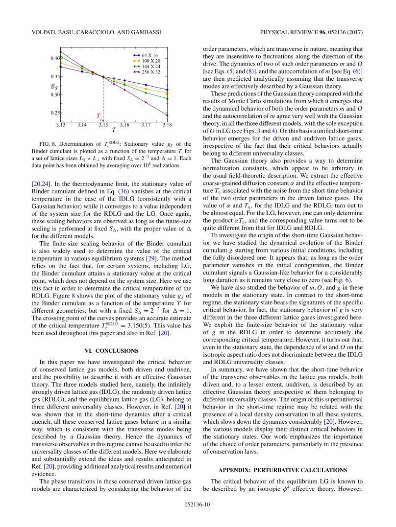
FIG. 8. Determination of T RDLGc : Stationary value gS of the

Binder cumulant is plotted as a function of the temperature T fora set of lattice sizes L‖ × L⊥ with fixed S� = 2−2 and � = 1. Eachdata point has been obtained by averaging over 108 realizations.

[20,24]. In the thermodynamic limit, the stationary value ofBinder cumulant defined in Eq. (36) vanishes at the criticaltemperature in the case of the IDLG (consistently with aGaussian behavior) while it converges to a value independentof the system size for the RDLG and the LG. Once again,these scaling behaviors are observed as long as the finite-sizescaling is performed at fixed S�, with the proper value of �

for the different models.The finite-size scaling behavior of the Binder cumulant

is also widely used to determine the value of the criticaltemperature in various equilibrium systems [29]. The methodrelies on the fact that, for certain systems, including LG,the Binder cumulant attains a stationary value at the criticalpoint, which does not depend on the system size. Here we usethis fact in order to determine the critical temperature of theRDLG. Figure 8 shows the plot of the stationary value gS ofthe Binder cumulant as a function of the temperature T fordifferent geometries, but with a fixed S� = 2−2 for � = 1.

The crossing point of the curves provides an accurate estimateof the critical temperature T RDLG

c = 3.150(5). This value hasbeen used throughout this paper and also in Ref. [20].

VI. CONCLUSIONS

In this paper we have investigated the critical behaviorof conserved lattice gas models, both driven and undriven,and the possibility to describe it with an effective Gaussiantheory. The three models studied here, namely, the infinitelystrongly driven lattice gas (IDLG), the randomly driven latticegas (RDLG), and the equilibrium lattice gas (LG), belong tothree different universality classes. However, in Ref. [20] itwas shown that in the short-time dynamics after a criticalquench, all these conserved lattice gases behave in a similarway, which is consistent with the transverse modes beingdescribed by a Gaussian theory. Hence the dynamics oftransverse observables in this regime cannot be used to infer theuniversality classes of the different models. Here we elaborateand substantially extend the ideas and results anticipated inRef. [20], providing additional analytical results and numericalevidence.

The phase transitions in these conserved driven lattice gasmodels are characterized by considering the behavior of the

order parameters, which are transverse in nature, meaning thatthey are insensitive to fluctuations along the direction of thedrive. The dynamics of two of such order parameters m and O

[see Eqs. (5) and (8)], and the autocorrelation of m [see Eq. (6)]are then predicted analytically assuming that the transversemodes are effectively described by a Gaussian theory.

These predictions of the Gaussian theory compared with theresults of Monte Carlo simulations from which it emerges thatthe dynamical behavior of both the order parameters m and O

and the autocorrelation of m agree very well with the Gaussiantheory, in all the three different models, with the sole exceptionof O in LG (see Figs. 3 and 4). On this basis a unified short-timebehavior emerges for the driven and undriven lattice gases,irrespective of the fact that their critical behaviors actuallybelong to different universality classes.

The Gaussian theory also provides a way to determinenormalization constants, which appear to be arbitrary inthe usual field-theoretic description. We extract the effectivecoarse-grained diffusion constant α and the effective tempera-ture Tη associated with the noise from the short-time behaviorof the two order parameters in the driven lattice gases. Thevalue of α and Tη, for the IDLG and the RDLG, turn out tobe almost equal. For the LG, however, one can only determinethe product αTη, and the corresponding value turns out to bequite different from that for IDLG and RDLG.

To investigate the origin of the short-time Gaussian behav-ior we have studied the dynamical evolution of the Bindercumulant g starting from various initial conditions, includingthe fully disordered one. It appears that, as long as the orderparameter vanishes in the initial configuration, the Bindercumulant signals a Gaussian-like behavior for a considerablylong duration as it remains very close to zero (see Fig. 6).

We have also studied the behavior of m,O, and g in thesemodels in the stationary state. In contrast to the short-timeregime, the stationary state bears the signatures of the specificcritical behavior. In fact, the stationary behavior of g is verydifferent in the three different lattice gases investigated here.We exploit the finite-size behavior of the stationary valueof g in the RDLG in order to determine accurately thecorresponding critical temperature. However, it turns out that,even in the stationary state, the dependence of m and O on theisotropic aspect ratio does not discriminate between the IDLGand RDLG universality classes.

In summary, we have shown that the short-time behaviorof the transverse observables in the lattice gas models, bothdriven and, to a lesser extent, undriven, is described by aneffective Gaussian theory irrespective of them belonging todifferent universality classes. The origin of this superuniversalbehavior in the short-time regime may be related with thepresence of a local density conservation in all these systems,which slows down the dynamics considerably [20]. However,the various models display their distinct critical behaviors inthe stationary states. Our work emphasizes the importanceof the choice of order parameters, particularly in the presenceof conservation laws.

APPENDIX: PERTURBATIVE CALCULATIONS

The critical behavior of the equilibrium LG is known tobe described by an isotropic φ4 effective theory. However,

052136-10

UNIVERSAL GAUSSIAN BEHAVIOR OF DRIVEN LATTICE . . . PHYSICAL REVIEW E 96, 052136 (2017)

the behavior of the Binder cumulant g measured in MonteCarlo simulations (see Fig. 6) is seemingly consistent with theGaussian theory in the short-time regime following a criticalquench. To understand this surprising fact, we perform a first-order perturbative calculation of the Binder cumulant for theLG. For simplicity, we assume the lattice to be sufficientlylarge to replace it with a continuum.

The time evolution of the coarse-grained spin field φ(x,t) inLG is governed by the Langevin equation (9) where u denotesthe strength of the perturbation. To linear order in u,

φ(x,t) = φ0(x,t) + uφ1(x,t), (A1)

where φ0(x,t) is the solution of Eq. (9) with u = 0 (Gaussian)and φ1(x,t) is the perturbative correction. It is useful to recallthat the Fourier transform φ0

k (t) of φ0(x,t) is the continuumversion of Eq. (16), i.e.,

φ0k (t) = ik

∫ t

0dsηk(s)e−γk (t−s), (A2)

where γk = αk2(τ + k2) [see Eq. (14) with k̂ → k], and ηk

is the white noise on the continuum with 〈ηk(t)ηk′(t ′)〉 =2αTη(2π )dδ(k + k′)δ(t − t ′). The time evolution of the Fouriertransform φ1

k (t) of the linear correction φ1(x,t) follows fromEq. (9), which takes the form

d

dtφ1

k (t) = −γkφ1k (t) − αk2fk(t), (A3)

where fk(t) is the Fourier transform of [φ0(x,t)]3, i.e.,

fk(t) =∫

dk1

(2π )ddk2

(2π )dφ0

k−k1(t)φ0

k1−k2(t)φ0

k2(t). (A4)

Equation (A3) can be solved and yields,

φ1k (t) = −αk2

∫ t

0dse−γk (t−s)fk(s). (A5)

To compute the Binder cumulant of the kth mode, as defined inEq. (36), we need to evaluate the second and fourth moment ofφk(t). For the Gaussian theory, the Binder cumulant g vanisheswhile, to the leading order in u it takes the value

g = u

[4δ2

〈|φ0k |2〉

− δ4

〈|φ0k |2〉2

], (A6)

where the coefficients δ2 and δ4 are correlations between theGaussian field φ0 with the linear correction φ1:

δ2 = ⟨φ0

kφ1−k

⟩ + ⟨φ0

−kφ1k

⟩δ4 = 2

[⟨φ0

kφ0−kφ

0−kφ

1k

⟩ + ⟨φ0

kφ0kφ

0−kφ

1−k

⟩]. (A7)

Here all the fields φ0k and φ1

k are evaluated at the same timet. Since φ1

k contains product of three φ0k s, δ2, and δ4 are four-

and six-point correlations of the Gaussian field, which can beevaluated via Wick’s theorem. The two contributions in δ4 areconnected by a k → −k exchange and it is straightforward tosee that

δ4 = 4〈|φ0k |2〉δ2 − 4g̃, (A8)

where g̃ contains the contributions from the connected terms,i.e., terms in which each φ0

k (t) is contracted with a φ0k′(s) for a

time t > s. There are six such connected contributions, which

can be obtained explicitly from Eqs. (A4) and (A5). It is easyto see that they all contribute the same and we finally get

g̃ = 6αk2∫ t

0dse−γk (t−s)

∫dk1

(2π )ddk2

(2π )d

× ⟨φ0

k (t)φ0k−k1

(s)⟩⟨φ0

−k(t)φ0k1−k2

(s)⟩⟨φ0

−k(t)φ0k2

(s)⟩. (A9)

The autocorrelation of the Gaussian field φ0k (t) is directly

obtained from Eq. (A2),

⟨φ0

k (t)φ0k′(s)

⟩ = αTη

(2π )dk2

γk

e−γk (t−s)(1 − e−2γks)δ(k + k′)

(A10)

for t > s. Using Eq. (A10), the momentum integrals inEq. (A9) can be calculated, and, at the critical point (i.e.,with γk = αk4) we get,

g̃ = 6αT 3η (2π )d

k4e−4αk4t

∫ t

0dseαk4s

(eαk4s − e−αk4s

)3

= 6T 3η (2π )d

k8

[1

4+ 1

2e−6αk4t + 3e−4αk4t

(1

4+ αk4t

)

− 3

2e−2αk4t

]. (A11)

Finally, combining Eqs. (A6), (A8), and (A11) we get thelinear correction to the Binder cumulant for a φ4 theory,

g = 4ug̃

〈|φ0k |2〉2

= 24uTη

(2π )dk4

1(1 − e−2αk4t

)2

[1

4+ 1

2e−6αk4t

+ 3e−4αk4t

(1

4+ αk4t

)− 3

2e−2αk4t

].

(A12)

We are particularly interested in the behavior of g in theshort-time regime, which can be obtained by expanding theexponential in Eq. (A12) and by keeping the lowest-orderterms in t. It turns out that the Binder cumulant growsquadratically upon increasing t,

g ∼ k4t2 + O(t3). (A13)

In order to appreciate the role of the local conservation of φ itis useful to repeat this calculation for the nonconserved field,in which case γk = αk2 at the critical point. Following thesame steps, one finds,

g ∼ t2 + O(t3). (A14)

This lowest-order perturbative calculation is strictly validaround the upper critical dimensionality dc = 4 of the model.However, the qualitative feature that is of importance here isthe fact that in the conserved case in Eq. (A13) the growth ofg is reduced by a factor of k4 compared to the nonconservedcase in Eq. (A14). For the first mode on a large lattice of linearsize L, k ∼ 1/L and hence g appears to be vanishingly smallfor the LG. This heuristic calculation provides a way to seehow drastically conservation can alter the dynamical behaviorof a system.

052136-11

VOLPATI, BASU, CARACCIOLO, AND GAMBASSI PHYSICAL REVIEW E 96, 052136 (2017)

[1] L. P. Kadanoff, in Critical Phenomena, Proceedings of the Int.School of Physics, Enrico Fermi, Course LI, edited by M. S.Green (Academic Press, New York, 1971).

[2] U. C. Täuber, Critical Dynamics: A Field Theory Approachto Equilibrium and Non-Equilibrium Scaling Behavior (Cam-bridge University Press, Cambridge, 2014).

[3] P. Hohenberg and B. I. Halperin, Rev. Mod. Phys. 49, 435 (1977).[4] J. Cardy and U. C. Täuber, Phys. Rev. Lett. 77, 4780 (1996).[5] M. Kardar, G. Parisi, and Y. C. Zhang, Phys. Rev. Lett. 56, 889

(1986).[6] H. K. Janssen, B. Schaub, and B. Schmittmann, Z. Phys. B 73,

539 (1989).[7] B. Zheng, Int. J. Mod. Phys. B 12, 1419 (1998).[8] E. V. Albano et. al., Rep. Prog. Phys. 74, 026501 (2011).[9] E. V. Albano and G. Saracco, Phys. Rev. Lett. 88, 145701 (2002).

[10] G. L. Daquila and U. C. Täuber, Phys. Rev. Lett. 108, 110602(2012).

[11] J. Marro and R. Dickman, Nonequilibrium Phase Transitions inLattice Models (Cambridge University Press, Cambridge, 2005).

[12] B. Schmittmann and R. K. P. Zia, in Statistical Mechanics ofDriven Diffusive Systems, edited by C. Domb and J. L. Lebowitz,Phase Transitions and Critical Phenomena Vol. 17 (AcademicPress, London, 1995).

[13] H. Tanaka, J. Phys.: Condens. Matter 12, R207 (2000).[14] D. Chowdhury, L. Santen, and A. Schadschneider, Phys. Rep.

329, 199 (2000).[15] J. Stenhammar, A. Tiribocchi, R. J. Allen, D. Marenduzzo, and

M. E. Cates, Phys. Rev. Lett. 111, 145702 (2013).[16] R. Wittkowski, A. Tiribocchi, J. Stenhammar, R. J. Allen, D.

Marenduzzo, and M. E. Cates, Nat. Commun. 5, 4351 (2014).

[17] G. Mussardo, Statistical Field Theory: An Introduction toExactly Solved Models in Statistical Physics (Oxford UniversityPress, Oxford, 2010).

[18] S. Katz, J. L. Lebowitz, and H. Spohn, Phys. Rev. B 28, 1655(R)(1983); J. Stat. Phys. 34, 497 (1984).

[19] B. Schmittmann, Europhys. Lett. 24, 109 (1993).[20] U. Basu, V. Volpati, S. Caracciolo, and A. Gambassi, Phys. Rev.

Lett. 118, 050602 (2017).[21] R. J. Baxter, Exactly Solved Models in Statistical Mechanics

(Academic Press, London, 1982).[22] H. K. Janssen and B. Schmittmann, Z. Phys. B 64, 503 (1986).[23] K.-t. Leung and J. L. Cardy, J. Stat. Phys. 44, 567 (1986).[24] S. Caracciolo, A. Gambassi, M. Gubinelli, and A. Pelissetto,

J. Phys. A 36, L315 (2003).[25] S. Caracciolo, A. Gambassi, M. Gubinelli, and A. Pelissetto,

Phys. Rev. E 72, 056111 (2005).[26] R. Kubo, Rep. Prog. Phys. 29, 255 (1966).[27] M. Abramowitz and I. A. Stegun, Handbook of Mathematical

Functions (Dover, New York, 1972).[28] A. Gut, An Intermediate Course in Probability (Springer,

New York, 2009).[29] K. Binder and D. Heermann, Monte Carlo Simulation in

Statistical Physics (Springer-Verlag, Berlin, 2010).[30] S. Caracciolo, A. Gambassi, M. Gubinelli, and A. Pelissetto,

J. Stat. Phys. 115, 281 (2004).[31] C. Godrèche, F. Krzakała, and F. Ricci-Tersenghi, J. Stat. Mech.

(2004) P04007.[32] Note, however, that if the same quantities are plotted as functions

of only the orthogonal lattice size L⊥, the two models areexpected to be distinguishable according to Eq. (38).

052136-12