Universal structure of covariant holographic two-point functions inmassless higher-order gravities

Yue-Zhou Li, H. Lu and Zhan-Feng Mai

Yukawa Institute of Theoretical Physics (YITP)

11th, February, 2019

Abstract and main result

We manily consider massless high-order gravities in general D = d + 1 dimensions,which are Einstein gravity extended with higher-order curvature invariants in such away that the linearized spectrum around the AdS vacca involes only the masslessgraviton. We derive the covariant holographic two-point function and find that theyhave a universal structure.

the theory-dependent overall coefficient factor CT can be universally expressedby (d − 1)CT = `(∂a/∂`), where a is the holographic a-charge and ` is the AdSradius.

We verify this relations in Gauss-Bonnet, Lovelock and Einstein cubic gravities.

In d = 4, we also find an intriguing relation between the holographic c and acharges, namely c = 1

3 `∂a∂`

, which implies CT = c.

Introduction

According to the basic idea of the AdS/CFT Correspondence providing a moremanageable approach to compute n-point functions is the field-operator duality. Theboundary value φ0 of φ is identified as the source coupled to the operator, andfurthermore the partition function of the boundary CFTd is identified with theon-shell action of AdSd+1 gravities

Sgr|φ0 =< exp(−∫

ddxφ0Oφ) > . (1)

With the identification, the n-point function of the operator Oφ of the CFTd can becomputed by evaluating on-shell action of the gravity theories:

< Oφ(x1) · · · Oφ(xn) >=δnS

δφ0(x1) · · · δφ0(xn). (2)

In pure gravities, the only available field is the metric, and the correspondingoperator is the energy-momentum tensor of the boundary CFT. The correspondingtwo-point functions in Einstein gravity in general dimensions were previouslyobtained.[hep-th/9804083]

Introduction

In this paper, we compute covariant holographic two-point functions in masslesshigher-order gravities. We mainly follow the method of[Arxiv:1205.5804][Arxiv:1411.3158]developed for four dimensions. We generalizedto general D = d + 1 dimensions and obtain that

< Tij(x)Tkl(0) >=N2CTIijkl(x)

x2d . (3)

where N2 is a numerical constant depending only on d. The boundary spacetimetensor Iijkl(x) is defined by

Iijkl =12

(IikIjl + IilIjk) −1dηijηkl (4)

Iij = ηij −2xixj

x2 . (5)

where xi are the cartesian coodinates of the boundary Minkowski spacetime ηij. Thestructure matches the result ofCFT[hep-th/930710][hep-th/96050009][Arxiv:1203.1339], and also matches theresult of Einstein gravity and Gauss-Bonnet Gravity [Arxiv:0911.4257]

Introduction

The coefficient CT depend on the detail of the theory, however, for masslesshigher-order gravities, we find that there is a universal expression relating CT toa-charge:

CT =1

d − 1`∂a∂`

(6)

where a is the coefficient of the Euler density in the holographic conformalanomaly.(See,e,g.[hep-th/9806087][hep-th/9812032][hep-th/9910267])The parameter ` is the radius of the AdS vacuum. It is important to emphasize thatthe a-charge must be expressed in terms of the ` and the bare coupling constants ofthe higher-curvature invariants as independent parameters, with the barecosmological constant Λ0 solved in terms of thesed quantities by the E.O.M.

The covariant structure of two-point functions

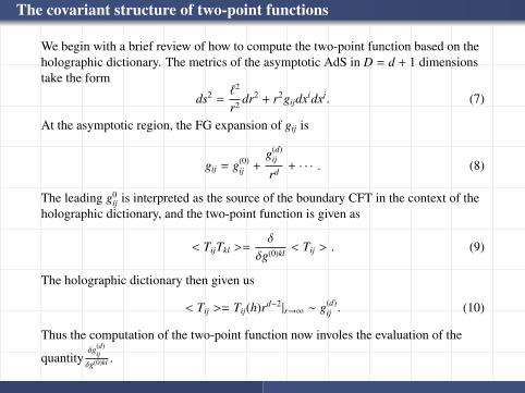
We begin with a brief review of how to compute the two-point function based on theholographic dictionary. The metrics of the asymptotic AdS in D = d + 1 dimensionstake the form

ds2 =`2

r2 dr2 + r2gijdxidxj. (7)

At the asymptotic region, the FG expansion of gij is

gij = g(0)ij +

g(d)ij

rd + · · · . (8)

The leading g0ij is interpreted as the source of the boundary CFT in the context of the

holographic dictionary, and the two-point function is given as

< TijTkl >=δ

δg(0)kl < Tij > . (9)

The holographic dictionary then given us

< Tij >= Tij(h)rd−2|r→∞ ∼ g(d)ij . (10)

Thus the computation of the two-point function now involes the evaluation of the

quantityδg(d)

ij

δg(0)kl .

The covariant structure of two-point functions

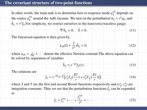
In other words, the main task is to determine how to response mode g(d)ij depends on

the source g(0)ij around the AdS vacuum. We turn on the perturbation hij = r2ηij, and

hij = r2fij.For simplicity, we restrict ourselves to the transverse-traceless gauge:

∇jhij = 0, h = 0. (11)

The linearized equation is then given by

κeff(� +2`2 )hij = 0. (12)

where κeff = 116π + · · · denote the effective Newton constant.The above equation can

be solved by separation of variables

hij = e−ipxfij(r). (13)

The solutions arefij = e−iEtr−

d2(ca

ijJ d2

(E`r

)+ cb

ijY d2

(E`r

))). (14)

where J and Y are the first and second Bessel functions respectively and (caij, c

bij) are

integration constants. Thus we see that the perturbation functions fij can be expandedas

fij = f (0)ij + · · · +

f (d)ij

rd + · · · . (15)

The covariant structure of two-point functions

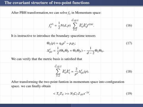
After PBH transformation,we can solve fij in Momentum space:

f (d)ij =

12

N(d, p)

d2+d−42∑

I=d

EIklE

Iijf

(0)kl. (16)

It is instructive to introduce the boundary spacetime tensors

Θij(p) = ηijp2 − pipj; (17)

∆dijkl =

12

(ΘikΘjl + ΘilΘjk) −1

d − 2ΘijΘkl.

We can verify that the metric basis is satisfied that

d2+d−42∑

I=d

EIklE

Jij =

2p4 ∆d

ijkl(p). (18)

After transforming the two-point funtion in momentum space into configurationspace. we can finally obtain

< TijTkl >= N2CTIijklx−2d. (19)

The covariant structure of two-point functions

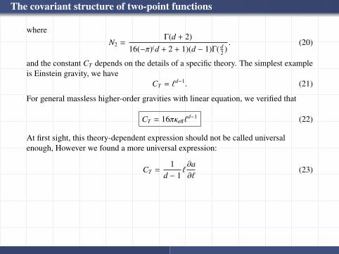
whereN2 =

Γ(d + 2)16(−π)(d + 2 + 1)(d − 1)Γ( d

2 ). (20)

and the constant CT depends on the details of a specific theory. The simplest exampleis Einstein gravity, we have

CT = `d−1. (21)

For general massless higher-order gravities with linear equation, we verified that

CT = 16πκeff`d−1 (22)

At first sight, this theory-dependent expression should not be called universalenough, However we found a more universal expression:

CT =1

d − 1`∂a∂`

(23)

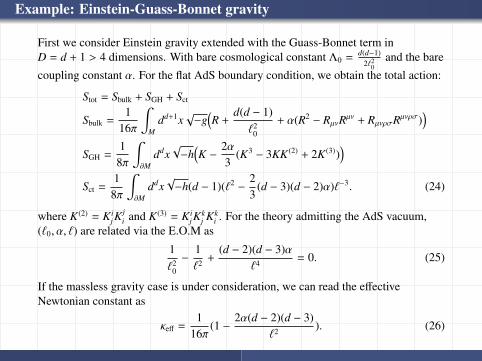
Example: Einstein-Guass-Bonnet gravity

First we consider Einstein gravity extended with the Guass-Bonnet term inD = d + 1 > 4 dimensions. With bare cosmological constant Λ0 =

d(d−1)2`2

0and the bare

coupling constant α. For the flat AdS boundary condition, we obtain the total action:

Stot = Sbulk + SGH + Sct

Sbulk =1

16π

∫M

dd+1x√−g

(R +

d(d − 1)`2

0

+ α(R2 − RµνRµν + RµνρσRµνρσ))

SGH =1

8π

∫∂M

ddx√−h

(K −

2α3

(K3 − 3KK(2) + 2K(3)))

Sct =1

8π

∫∂M

ddx√−h(d − 1)(`2 −

23

(d − 3)(d − 2)α)`−3. (24)

where K(2) = Kij K

ji and K(3) = Ki

j Kkj Kk

i . For the theory admitting the AdS vacuum,(`0, α, `) are related via the E.O.M as

1`2

0

−1`2 +

(d − 2)(d − 3)α`4 = 0. (25)

If the massless gravity case is under consideration, we can read the effectiveNewtonian constant as

κeff =1

16π(1 −

2α(d − 2)(d − 3)`2 ). (26)

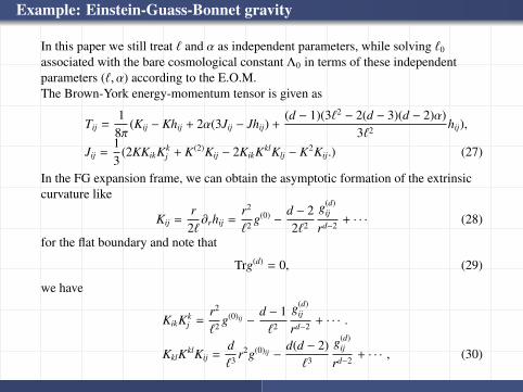
Example: Einstein-Guass-Bonnet gravity

In this paper we still treat ` and α as independent parameters, while solving `0

associated with the bare cosmological constant Λ0 in terms of these independentparameters (`, α) according to the E.O.M.The Brown-York energy-momentum tensor is given as

Tij =1

8π(Kij − Khij + 2α(3Jij − Jhij) +

(d − 1)(3`2 − 2(d − 3)(d − 2)α)3`2 hij),

Jij =13

(2KKikKkj + K(2)Kij − 2KikKklKlj − K2Kij.) (27)

In the FG expansion frame, we can obtain the asymptotic formation of the extrinsiccurvature like

Kij =r

2`∂rhij =

r2

`2 g(0) −d − 22`2

g(d)ij

rd−2 + · · · (28)

for the flat boundary and note that

Trg(d) = 0, (29)

we have

KikKkj =

r2

`2 g(0)ij −d − 1`2

g(d)ij

rd−2 + · · · .

KklKklKij =d`3 r2g(0)ij −

d(d − 2)`3

g(d)ij

rd−2 + · · · , (30)

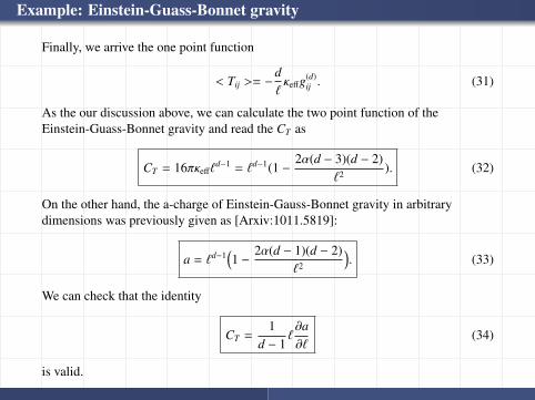
Example: Einstein-Guass-Bonnet gravity

Finally, we arrive the one point function

< Tij >= −d`κeffg(d)

ij . (31)

As the our discussion above, we can calculate the two point function of theEinstein-Guass-Bonnet gravity and read the CT as

CT = 16πκeff`d−1 = `d−1(1 −

2α(d − 3)(d − 2)`2 ). (32)

On the other hand, the a-charge of Einstein-Gauss-Bonnet gravity in arbitrarydimensions was previously given as [Arxiv:1011.5819]:

a = `d−1(1 −

2α(d − 1)(d − 2)`2

). (33)

We can check that the identity

CT =1

d − 1`∂a∂`

(34)

is valid.

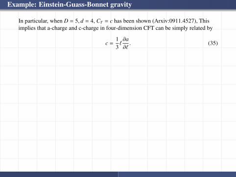
Example: Einstein-Guass-Bonnet gravity

In particular, when D = 5, d = 4, CT = c has been shown (Arxiv:0911.4527), Thisimplies that a-charge and c-charge in four-dimension CFT can be simply related by

c =13`∂a∂`. (35)

Example: Einstein-Lovelock Gravities

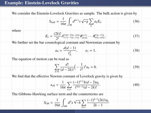
We consider the Einstein-Lovelock Gravities as sample. The bulk action is given by

Sbulk =1

16π

∫M

dd+1x√−g

∑k

akEk. (36)

whereEk =

(2k)!2k δ

µ1µ2 ···µ2k−1µ2kν1ν2 ···ν2k−1ν2k Rν1ν2

µ1µ2· · ·Rν2k−1ν2k

µ2k−1µ2k . (37)

We further set the bar cosmological constant and Newtonian constant by

a0 =d(d − 1)

`20

, a1 = 1. (38)

The equation of motion can be read as∑k>0

d!(d − 2k)!

(−

1`2 )kak = 0. (39)

We find that the effective Newton constant of Lovelock gravity is given by

κeff =1

16π

∑k≥1

(−1)k+1k(d − 2)ak

`2(k−1)(d − 2k)!. (40)

The Gibbons-Hawking surface term and the counterterms are

SGH =1

16π

∫∂M

ddx√−h

∑k≥1

(−1)k−1(2k)!ak

2k − 1

δi1 ···i2k−1j1 ···j2k−1

Kj1i1· · ·Kj2k−1

i2k−1(41)

Sct =1

16πddx√−h

∑k

2k(−1)k(d − 1)ak

(2k − 1)(d − 2k)!(1`

)2k−1.

Example: Einstein-Lovelock Gravities

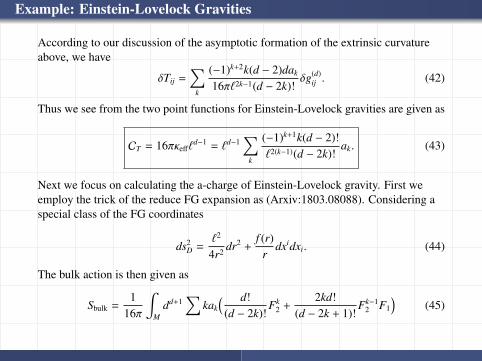
According to our discussion of the asymptotic formation of the extrinsic curvatureabove, we have

δTij =∑

k

(−1)k+2k(d − 2)dak

16π`2k−1(d − 2k)!δg(d)

ij . (42)

Thus we see from the two point functions for Einstein-Lovelock gravities are given as

CT = 16πκeff`d−1 = `d−1

∑k

(−1)k+1k(d − 2)!`2(k−1)(d − 2k)!

ak. (43)

Next we focus on calculating the a-charge of Einstein-Lovelock gravity. First weemploy the trick of the reduce FG expansion as (Arxiv:1803.08088). Considering aspecial class of the FG coordinates

ds2D =

`2

4r2 dr2 +f (r)

rdxidxi. (44)

The bulk action is then given as

Sbulk =1

16π

∫M

dd+1∑

kak

( d!(d − 2k)!

Fk2 +

2kd!(d − 2k + 1)!

Fk−12 F1

)(45)

Example: Einstein-Lovelock Gravities

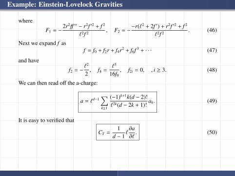
where

F1 = −2r2ff ′′ − r2f ′2 + f 2

`2f 2 , F2 = −−r(`2 + 2f ′) + r2f ′2 + f 2

`2f 2 . (46)

Next we expand f asf = f0 + f2r + f4r2 + f6f 3 + · · · (47)

and have

f2 = −`2

2, f4 =

`3

16f0, f2i = 0, , i ≥ 3. (48)

We can then read off the a-charge:

a = `d−1∑k≥1

(−1)k+1k(d − 2)!`2k(d − 2k + 1)!

ak. (49)

It is easy to verified that

CT =1

d − 1`∂a∂`. (50)

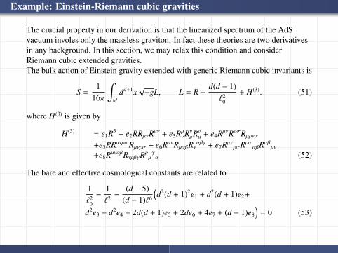
Example: Einstein-Riemann cubic gravities

The crucial property in our derivation is that the linearized spectrum of the AdSvacuum involes only the massless graviton. In fact these theories are two derivativesin any background. In this section, we may relax this condition and considerRiemann cubic extended gravities.The bulk action of Einstein gravity extended with generic Riemann cubic invariants is

S =1

16π

∫M

dd+1x√−gL, L = R +

d(d − 1)`2

0

+ H(3). (51)

where H(3) is given by

H(3) = e1R3 + e2RRµνRµν + e3RµνR

νρR

ρµ + e4RµνRρσRµρνσ

+e5RRµνρσRµνρσ + e6RµνRµαβRναβγ + e7Rµν

ρσRρσαβRαβ

µν

+e8RµναβRνρβγRρµγα (52)

The bare and effective cosmological constants are related to

1`2

0

−1`2 −

(d − 5)(d − 1)`6

(d2(d + 1)2e1 + d2(d + 1)e2+

d2e3 + d2e4 + 2d(d + 1)e5 + 2de6 + 4e7 + (d − 1)e8

)= 0 (53)

Example: Einstein-Riemann cubic gravities

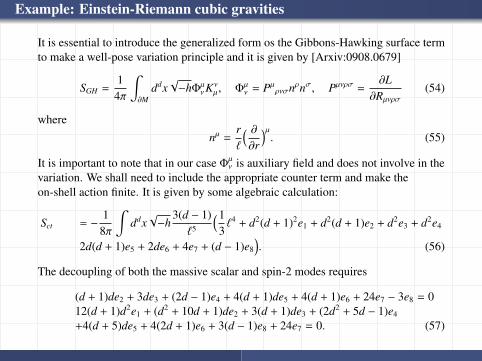
It is essential to introduce the generalized form os the Gibbons-Hawking surface termto make a well-pose variation principle and it is given by [Arxiv:0908.0679]

SGH =1

4π

∫∂M

ddx√−hΦµ

νKνµ, Φµ

ν = Pµρνσnρnσ, Pµνρσ =

∂L∂Rµνρσ

(54)

wherenµ =

r`

( ∂∂r

)µ. (55)

It is important to note that in our case Φµν is auxiliary field and does not involve in the

variation. We shall need to include the appropriate counter term and make theon-shell action finite. It is given by some algebraic calculation:

Sct = −1

8π

∫ddx√−h

3(d − 1)`5

(13`4 + d2(d + 1)2e1 + d2(d + 1)e2 + d2e3 + d2e4

2d(d + 1)e5 + 2de6 + 4e7 + (d − 1)e8

). (56)

The decoupling of both the massive scalar and spin-2 modes requires

(d + 1)de2 + 3de3 + (2d − 1)e4 + 4(d + 1)de5 + 4(d + 1)e6 + 24e7 − 3e8 = 012(d + 1)d2e1 + (d2 + 10d + 1)de2 + 3(d + 1)de3 + (2d2 + 5d − 1)e4

+4(d + 5)de5 + 4(2d + 1)e6 + 3(d − 1)e8 + 24e7 = 0. (57)

Example: Einstein-Riemann cubic gravities

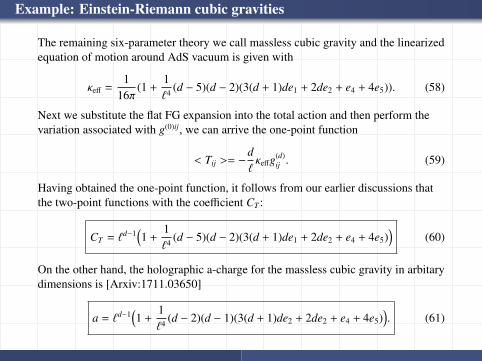
The remaining six-parameter theory we call massless cubic gravity and the linearizedequation of motion around AdS vacuum is given with

κeff =1

16π(1 +

1`4 (d − 5)(d − 2)(3(d + 1)de1 + 2de2 + e4 + 4e5)). (58)

Next we substitute the flat FG expansion into the total action and then perform thevariation associated with g(0)ij, we can arrive the one-point function

< Tij >= −d`κeffg(d)

ij . (59)

Having obtained the one-point function, it follows from our earlier discussions thatthe two-point functions with the coefficient CT :

CT = `d−1(1 +

1`4 (d − 5)(d − 2)(3(d + 1)de1 + 2de2 + e4 + 4e5)

)(60)

On the other hand, the holographic a-charge for the massless cubic gravity in arbitarydimensions is [Arxiv:1711.03650]

a = `d−1(1 +

1`4 (d − 2)(d − 1)(3(d + 1)de2 + 2de2 + e4 + 4e5)

). (61)

Example: Einstein-Riemann cubic gravities

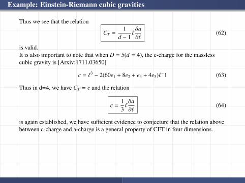
Thus we see that the relation

CT =1

d − 1`∂a∂`

(62)

is valid.It is also important to note that when D = 5(d = 4), the c-charge for the masslesscubic gravity is [Arxiv:1711.03650]

c = `3 − 2(60e1 + 8e2 + e4 + 4e5)`−1 (63)

Thus in d=4, we have CT = c and the relation

c =13`∂a∂`

(64)

is again established, we have sufficient evidence to conjecture that the relation abovebetween c-charge and a-charge is a general property of CFT in four dimensions.

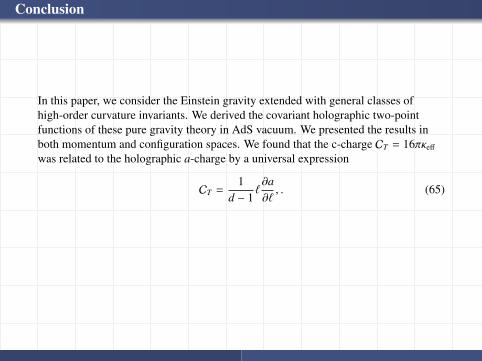
Conclusion

In this paper, we consider the Einstein gravity extended with general classes ofhigh-order curvature invariants. We derived the covariant holographic two-pointfunctions of these pure gravity theory in AdS vacuum. We presented the results inboth momentum and configuration spaces. We found that the c-charge CT = 16πκeff

was related to the holographic a-charge by a universal expression

CT =1

d − 1`∂a∂`, . (65)