Embed Size (px)
Citation preview
UNIVERSIDAD SAN FRANCISCO DE QUITO USFQ
Colegio de Administracion y Economıa
Political Instability and Economic Growth in Ecuador
An empirical analysis
Proyecto de Investigacion
Johanna Estefania Andrango Brito
Economıa
Trabajo de titulacion presentado como requisito
para la obtencion del tıtulo de
Economista
Quito, 21 de diciembre de 2016

2
UNIVERSIDAD SAN FRANCISCO DE QUITO USFQ
COLEGIO DE ADMINISTRACION Y ECONOMIA
HOJA DE CALIFICACIONDE TRABAJO DE TITULACION
Political instability and Economic Growth in Ecuador:An empirical analysis
Johanna Estefania Andrango Brito
Calificacion:
Nombre del profesor, Tıtulo academico:
Firma del profesor:
. . . . . . . . . . . . . . . . . . . . . . . .
Diego Grijalva, Ph.D.
. . . . . . . . . . . . . . . . . . . . . . . .
Quito, 21 de diciembre 2016

3
Derechos de Autor
Por medio del presente documento certifico que he leıdo todas las Polıticas y Manuales de la
Universidad San Francisco de Quito, incluyendo la Polıtica de Propiedad Intelectual USFQ, y
estoy de acuerdo con su contenido, por lo que los derechos de propiedad intelectual del presente
trabajo quedan sujetos a lo dispuesto en esas Polıticas.
Asimismo, autorizo a la USFQ para que realice la digitalizacion y publicacion de este tra-
bajo en el repositorio virtual, de conformidad a lo dispuesto en el Art. 144 de la Ley Organica
de Educacion Superior.
Firma del estudiante: . . . . . . . . . . . . . . . . . . . . . . . . . . . . . . . . . . . .
Nombres y Apellidos: Johanna Estefania Andrango Brito
Codigo: 00123309
Cedula de Identidad : 1718198151
Lugar y fecha: Quito, 21 diciembre de 2016

4
RESUMEN
Esta investigacion analiza la relacion endogena entre la inestabilidad polıtica y el crecimientoeconomico en Ecuador durante el periodo (1972-2013). Tras reconocer la multidimensionalidadde la inestabilidad polıtica se utilizo un Analisis de Componentes Principales (PCA) y se obtuvotres indices para esta variable: estabilidad democratica, inestabilidad del regimen y estabilidaddel gobierno. Igualmente, al tomar en cuenta la relacion endogena entre la inestabilidad polıticay crecimiento economico se utilizo un Modelo de Vectores Autoregresivos (VAR) y un Modelode Correcion de Errores de Vectores (VECM). Se evidencio que el unico ındice polıtico queafecta al crecimiento economico tanto en el corto como en el largo plazo es la estabilidad delgobierno. Este ındice presenta una relacion negativa en el corto plazo, pero una positiva en ellargo plazo. Por su parte, el crecimiento economico solo afecta en el corto plazo a la estabilidaddemocratica.
Palabras clave: Ecuador, inestabilidad polıtica, crecimiento economico, VECM, VAR

5
ABSTRACT
This paper analyzes the endogenous relationship between political instability and economicgrowth in Ecuador throughout the period 1972-2013. After acknowledging the multidimen-sional trait of political instability a Principal Component Analysis (PCA) was used and three po-litical instability index were obtained: democratic stability, regime instability and governmentstability. Additionally, taking into consideration the endogenous relation between the variablesboth Vector Error Correction Model (VECM) and Vector Autoregressive Model (VAR) wereapplied. There is evidence that the only political instability index that affects economic growthis government stability with a negative effect in the short run, but a positive effect in the longrun. Meanwhile, economic growth only affects in the short run the political index: democraticstability.
Keywords: Ecuador, political instability, economic growth, VECM, VAR

6
TABLE OF CONTENTS
LIST OF TABLES . . . . . . . . . . . . . . . . . . . . . . . . . . . . . . . . . . . . . 9
LIST OF FIGURES . . . . . . . . . . . . . . . . . . . . . . . . . . . . . . . . . . . . 10
1 Introduction . . . . . . . . . . . . . . . . . . . . . . . . . . . . . . . . . . . . . . 11
2 Literature Review . . . . . . . . . . . . . . . . . . . . . . . . . . . . . . . . . . . 12
3 Political Instability and Economic Growth in Ecuador- A historical perspective . 15
3.1 Presidents: political instability and the economy . . . . . . . . . . . . . . . . . 15
3.1.1 Jose Marıa Velasco Ibarra (1968-1972) . . . . . . . . . . . . . . . . . . 16
3.1.2 Guillermo Rodriguez Lara (1972-1976) . . . . . . . . . . . . . . . . . 17
3.1.3 Triumvirate (1976-1979) . . . . . . . . . . . . . . . . . . . . . . . . . 18
3.1.4 Jaime Roldos (1979-1981) . . . . . . . . . . . . . . . . . . . . . . . . 19
3.1.5 Osvaldo Hurtado (1981-1984) . . . . . . . . . . . . . . . . . . . . . . 20
3.1.6 Leoon Febres Cordero (1984-1988) . . . . . . . . . . . . . . . . . . . 22
3.1.7 Rodrigo Borja (1988-1992) . . . . . . . . . . . . . . . . . . . . . . . . 23
3.1.8 Sixto Duran Ballen (1992-1996) . . . . . . . . . . . . . . . . . . . . . 24
3.1.9 Abdala Bucaram (1996-1997) . . . . . . . . . . . . . . . . . . . . . . 25
3.1.10 Fabian Alarcon (1997-1998) . . . . . . . . . . . . . . . . . . . . . . . 26
3.1.11 Jamil Mahuad (1998-2000) . . . . . . . . . . . . . . . . . . . . . . . . 26
3.1.12 Gustavo Noboa (2000-2002) . . . . . . . . . . . . . . . . . . . . . . . 28
3.1.13 Lucio Gutierrez (2003-2005) . . . . . . . . . . . . . . . . . . . . . . . 28
3.1.14 Alfredo Palacio (2005-2006) . . . . . . . . . . . . . . . . . . . . . . . 30
3.1.15 Rafael Correa (2007-) . . . . . . . . . . . . . . . . . . . . . . . . . . . 30
4 Data and Empirical Model . . . . . . . . . . . . . . . . . . . . . . . . . . . . . . 32
4.1 Data . . . . . . . . . . . . . . . . . . . . . . . . . . . . . . . . . . . . . . . . 32
4.2 PCA Analysis . . . . . . . . . . . . . . . . . . . . . . . . . . . . . . . . . . . 32
4.2.1 PC1 Democratic stability . . . . . . . . . . . . . . . . . . . . . . . . . 35

7
4.2.2 PC2 Regime instability . . . . . . . . . . . . . . . . . . . . . . . . . . 36
4.2.3 PC3 Government stability . . . . . . . . . . . . . . . . . . . . . . . . 37
4.3 Specification of the Model . . . . . . . . . . . . . . . . . . . . . . . . . . . . 38
4.3.1 Model 1- Democratic stability . . . . . . . . . . . . . . . . . . . . . . 38
4.3.2 Results Model 1 . . . . . . . . . . . . . . . . . . . . . . . . . . . . . . 39
4.3.3 Model 2- Regime instability . . . . . . . . . . . . . . . . . . . . . . . 40
4.3.4 Results Model 2 . . . . . . . . . . . . . . . . . . . . . . . . . . . . . . 42
4.3.5 Model 3 - Government stability . . . . . . . . . . . . . . . . . . . . . . 42
4.3.6 Results Model 3 . . . . . . . . . . . . . . . . . . . . . . . . . . . . . . 43
5 Conclusions . . . . . . . . . . . . . . . . . . . . . . . . . . . . . . . . . . . . . . . 46
6 References . . . . . . . . . . . . . . . . . . . . . . . . . . . . . . . . . . . . . . . 47
Appendix A
Variables description . . . . . . . . . . . . . . . . . . . . . . . . . . . . . . . . . 51
Appendix B
PCA- Components Selection . . . . . . . . . . . . . . . . . . . . . . . . . . . . . 56
Appendix C
Unit root tests . . . . . . . . . . . . . . . . . . . . . . . . . . . . . . . . . . . . . 57
Appendix D
Cointegration tests . . . . . . . . . . . . . . . . . . . . . . . . . . . . . . . . . . . 58
Appendix E
Post estimation tests . . . . . . . . . . . . . . . . . . . . . . . . . . . . . . . . . . 59
E.1 Model 1 . . . . . . . . . . . . . . . . . . . . . . . . . . . . . . . . . . . . . . 59
E.1.1 Residual Autocorrelation . . . . . . . . . . . . . . . . . . . . . . . . . 59
E.1.2 Normally Distributed Disturbances . . . . . . . . . . . . . . . . . . . . 59
E.1.3 VAR Stability-Stationarity . . . . . . . . . . . . . . . . . . . . . . . . 60

8
E.2 Model 2 . . . . . . . . . . . . . . . . . . . . . . . . . . . . . . . . . . . . . . 60
E.2.1 Residual Autocorrelation . . . . . . . . . . . . . . . . . . . . . . . . . 60
E.2.2 Normally distributed disturbances . . . . . . . . . . . . . . . . . . . . 60
E.2.3 VAR Stability-Stationarity . . . . . . . . . . . . . . . . . . . . . . . . 61
E.3 Model 3 . . . . . . . . . . . . . . . . . . . . . . . . . . . . . . . . . . . . . . 61
E.3.1 Residual Autocorrelation . . . . . . . . . . . . . . . . . . . . . . . . . 61
E.3.2 Normally distributed disturbances . . . . . . . . . . . . . . . . . . . . 62
E.3.3 VECM Stability-Stationarity . . . . . . . . . . . . . . . . . . . . . . . 62

9
LIST OF TABLES
1 Descriptive statistics . . . . . . . . . . . . . . . . . . . . . . . . . . . . . . . . 33
2 Principal Component Analysis . . . . . . . . . . . . . . . . . . . . . . . . . . 34
3 Estimation results : VAR Model 1 . . . . . . . . . . . . . . . . . . . . . . . . 39
4 Estimation results : VAR 1974-2013 . . . . . . . . . . . . . . . . . . . . . . . 41
5 Estimation results: VECM 1974-2013 . . . . . . . . . . . . . . . . . . . . . . 44
6 Variables description . . . . . . . . . . . . . . . . . . . . . . . . . . . . . . . 51
7 Unit root tests . . . . . . . . . . . . . . . . . . . . . . . . . . . . . . . . . . . 57
8 Cointegration test Model 1 . . . . . . . . . . . . . . . . . . . . . . . . . . . . 58
9 Cointegration test Model 3 . . . . . . . . . . . . . . . . . . . . . . . . . . . . 58
10 Residual Autocorrelation Model 1 . . . . . . . . . . . . . . . . . . . . . . . . 59
11 Normally distributed disturbances tests . . . . . . . . . . . . . . . . . . . . . . 59
12 VAR Stability-Stationarity . . . . . . . . . . . . . . . . . . . . . . . . . . . . 60
13 Residual Autocrrelation Test Model 2 . . . . . . . . . . . . . . . . . . . . . . 60
14 Normally Distributed Disturbances Tests . . . . . . . . . . . . . . . . . . . . . 61
15 VAR Stability-Stationarity . . . . . . . . . . . . . . . . . . . . . . . . . . . . 61
16 Residual Autocrrelation Test Model 3 . . . . . . . . . . . . . . . . . . . . . . 62
17 Normally distributed disturbances tests . . . . . . . . . . . . . . . . . . . . . . 62
18 VECM Stability-Stationarity . . . . . . . . . . . . . . . . . . . . . . . . . . . 63

10
LIST OF FIGURES
1 Components derived from PCA . . . . . . . . . . . . . . . . . . . . . . . . . . 35
2 PCA scree plot test . . . . . . . . . . . . . . . . . . . . . . . . . . . . . . . . 56

11
1 Introduction
In general the relationship between politics and economics is crucial, since the former estab-
lishes the way a society is organized and the distribution of society’s resources through insti-
tutions. For example, at government level, leaders used instruments such a as fiscal policy and
monetary policy in order to influence the economic activity and reach political objectives such
as win elections or keep the power. In this sense political institutions affects the dynamics of
production, distribution and consumption of goods and services within a country. On the other
hand, economics is always a key variable that not only contributes to government stability, but
to the implementation or the maintenance of political institutions.
Specifically, Ecuador has suffered from long periods of political instability and volatile eco-
nomic growth. Regarding the former, since its foundations as a republic, Ecuador has registered
dictatorships, coups d’etat, anti-government demonstrations, disputes between the state powers,
massive strikes, among other political turmoil. Sometimes the same Ecuadorians considered
their country ungovernable, and each president has tried to “refound the country”. Meanwhile
economic activity in the Andean country has been driven by its commodity exports. Hence,
in a way Ecuador’s economic growth rates respond more to external forces rather than to a
sustainable economic plan figured by politicians. At the same time Ecuadorian presidents’ eco-
nomic management with a short term perspective and populist policies have been detrimental
to economic growth in the long run but contributed to government stability in the short run. In
this regard, it is important to analyze the relationship between these two variables in order to
understand which is an obstacle for the development of the other, and Ecuador’s development
per se.
In order to analyze this relationship between political instability and economic growth in the
case of Ecuador it is important to define political instability. Hence, due to the multidimensional
trait of this variable, a Principal Component Analysis was used. The different components
obtained were: democratic stability, regime instability and government stability. Additionally,
taking into consideration the endogeneity between economic growth and political instability
both Vector Autoregressive Model (VAR) and Vector Error Correction Model were applied. In

12
this research I found that the only political instability index that affects economic growth is
government stability with a negative effect in the short run, but a positive effect in the long run.
While, economic growth only affects politics through democratic stability.
This paper is organized as follows. The second section presents the literature review.
The third section analyzes the dynamics between political instability and economic growth in
Ecuador. The fourth section shows the data and the econometric models. The fifth section
concludes.
2 Literature Review
The relationship between political instability and economic growth has been extensively stud-
ied, since there is an important bidirectional link between the political environment and eco-
nomic activity. In this sense, many scholars suggest that there exists a negative effect of politi-
cal instability on economic growth (Barro, 1991; Barro & Lee, 1994; Mauro, 1995; Alesina &
Perotti, 1996; Perotti, 1996; Alesina et al., 1996; Chen & Feng, 1996; Asteriou & Price, 2000;
Carmignani, 2001; Jong-A-Pin, 2009). This effect is mainly caused by political uncertainty
which emerges after political turmoil affecting economic policy, the enforcement of property
rights and, eventually, repelling investment (Alesina & Perotti, 1996). Other scholars such as
Aisen & Veiga (2011) argue that the channels of transmission between political instability and
economic growth are through a lowering of the rates of productivity growth and, to a smaller
degree, physical and human capital accumulation.
In the same way, political instability contributes to the implementation of populist or myopic
policies that keep the leader in office, but are detrimental to economic growth (Carmignani,
2003; Herrera et al., 2015). Among these myopic policies are the creation of subsidies, the
increase of government expenditure, the delaying of structural reforms, devaluation contributing
to the trade-off between inflation and unmeployment (Carmignani, 2003). In fact, Grilli &
Tabellini (1991), Crain & Tollison (1993), Haan et al. (1999), Roubini & Sachs (1989) support
the existence of a positive relationship between deficits, debt accumulation and political turmoil.
Meanwhile, Annett (2000) and Darby et al. (2000) find the same correlation between political

13
instability and the share of total revenues used as government expenditure. This finding is in line
with the classical political business cycle theory, which sustains that in order for the incumbent
to stay in office, he will reduce unemployment below normal rates through the use of monetary
and fiscal policy; but, following the elections, an imminent rise in inflation is expected (Faust
& Irons, 1999).
Nevertheless, not all research supports the relationship between political instability and eco-
nomic growth. Levine & Renelt (1992), Benhabib & Spiegel (1997), Sala-i Martin (1997),
Svensson (1998), Campos & Nugent (2002), found no significant relationship between these
variables. Svensson (1998) in particular showed that controlling for the quality of property
rights, there is no effect from political instability on private investment and therefore on eco-
nomic growth. Additionally, Campos & Nugent (2002) separate the short term and long term
effects, and show that after taking away the Sub-Saharan African countries from the sample;
the long-run causal relationship between political instability and economic growth vanishes.
In Ecuador there has been a large descriptive research regarding the relationship between
these two variables, although no empirical analysis has been conducted yet. Schuldt (1994)
studied the political cycles during 1983-1994 and concluded that all Ecuadorian presidents in
that period used political cycles as an instrument to win elections or to boost their popularity.
Pachano (2007) and Freidenberg & Pachano (2016) agree and by means of a descriptive analysis
from 1979 to 2013 provide support to this perspective, establishing that most of the presidents
employed adjustment policies at the beginning of their periods but at the end they finished with
economic populist policies. Nevertheless, Polga & Mejia (2011) did not find any link between
economic performance and political instability, since the only case in which a president was
overthrown due to economic reasons was the coup d’etat against Jamil Mahuad. The two other
coups d’etat analyzed in his paper –Bucaram and Gutierrez– respond more to political reasons
than to economic motivations. Polga & Mejia (2011) argue that during the fall of Bucaram from
power the link between economic activity and political instability was weak, while Gutierrez
was overthrown during an economic boom. However, in a new research Basabe & Polga (2017)
establish that the necessary condition for a coup d’etat take place is social turmoil.
When defining political instability, the problem that arises is the different dimensions this

14
variable can present. In fact, there exist political dynamics beyond the probability of a govern-
ment change such as: political polarization, ethnic fragmentation, regime stability, government
stability, violence, among others (Alesina & Perotti, 1996; Feng, 1997; Aisen & Veiga, 2011;
Jong-A-Pin, 2009). Hence, to consider just one variable as a measure of political instability
limits the scope of analysis. In this sense, there are several indicators that take into consid-
eration multiple political variables to represent the different dimensions of political instability
(Alesina & Perotti, 1996; Campos & Nugent, 2002; Jong-A-Pin, 2009; Aisen & Veiga, 2011).
In order to capture these dimensions, one of the most frequent tools used is principal component
analysis (PCA) which reduces the multiple variables proxies of political instability into a few
components (Alesina & Perotti, 1996; Campos & Nugent, 2002; Aisen & Veiga, 2011).
In addition to the multidimensionality of political instability, when analyzing the relation-
ship between political instability and growth, the problem of endogeneity emerges. This means
that, on the one hand, poor economic conditions can lead to the emergence of political insta-
bility; but that, on the other hand, political instability can negatively affect economic growth.
In this sense, there is a bidirectional relation of causality between these two variables. Sev-
eral studies analyze the endogeneity relationship concluding that there is little evidence that
political instability Granger causes economic growth (Alesina et al., 1996). Since the relation-
ship between these two variables only appear when adding to the research Sub-Saharan African
countries (Campos & Nugent, 2002). However, other show evidence of the relationship be-
tween these two variables and finds that causation goes from economic growth towards political
violence (Jong-A-Pin, 2009).
Finally, regarding the methodology used in order to solve the problem of reverse causation,
one solution has been the use of simultaneous equations (Alesina & Perotti, 1996; Chen & Feng,
1996; Feng, 1997; Svensson, 1998; Annett, 2000). However, recent studies have employed
techniques such as the Generalized Methods of Moments (GMM) (Jong-A-Pin, 2009; Aisen &
Veiga, 2011). Most of these analyses, however, use panel data. When focusing on a country-
specific analysis techniques such as the GMM does not apply. In this sense, other methods
such as Vector Autoregressive Models (VAR) have been used when analyzing political business
cycles in the US (Faust & Irons, 1999). Campos & Karanasos (2007) use a Power ARCH model
15
to disentangle the relationship between growth, and political instability in Argentina. Asteriou
& Price (2000) employ a GARCH Model when analyzing the interaction of these two variables
in the UK. Hence, different approaches have been used to address the problem of endogeneity
between political instability and economic growth.
3 Political Instability and Economic Growth in Ecuador- A
historical perspective
Political instability has been a constant throughout Ecuadorian history. Since Ecuador’s foun-
dation as a republic in 1830, its polity has been characterized by coups d’etat, the creation
of new constitutions, the fragmentation of political parties, political personalization, conflicts
of interest between the Legislative and the Executive powers, lack of support and represen-
tation of the Executive power in Congress, and volatility in economic growth rates. In fact,
Ecuador has had twenty constitutions that on average lasted nine years ruling over two presi-
dential terms(Andrango et al., 2016). This political instability is not different from Ecuador’s
economic activity, since its economic growth responds mainly to the volatility of the commodity
prices that constitute its main exports. During the 1930s, Ecuador’s economy relied heavily on
the exports of cocoa beans, during the 50s on bananas and since 1972 on oil. In this sense, one
factor that explains the existing periods of political stability has been the significant resources
obtained from high commodity prices. These resources had been used by most of Ecuadorians
presidents, or military leaders had in order to influence the economy and stay in power.
3.1 Presidents: political instability and the economy
In the following section each presidential period since 1968 to 2013 will be analyzed. The start
point of analysis is 1968, since is the beginning of Jose Marıa Velasco Ibarra’s mandate, which
was in power in 1972, the beginning of the period analyzed in this paper. Thus, in order to
analyze his presidential mandate, his complete period was included in the descriptive analysis.

16
3.1.1 Jose Marıa Velasco Ibarra (1968-1972)
In 1968, Velasco Ibarra, the politician considered to be the most populist president of Ecuado-
rian history, was elected President for the fifth time with 32.8% of the votes. Among his propos-
als he promised to “achieve economic and social equality, eliminate the peasants’ humiliating
conditions, monitor oil contracts, and centralize the government” (Espinosa, 2000). Neverthe-
less, from the beginning of his mandate, Velasco faced political turmoil. One of the factors that
boosted his government political instability was the major changes in his cabinet. Specifically,
regarding the removal of four ministers of finance in the first two years of his government. The
first minister to be changed was the ministry of Agriculture due to the imposition of a tax to
sugar exports. In the same way, three out of the four removed ministers of finance were deposed
because of conflict of interests. The first minister was removed since he tried to increase income
tax collections, the second was changed because of lack of expertise, the third one tried to com-
bat smuggling in customs, and the forth was removed because he applied economic reforms in
order to correct the fiscal deficit.
Regarding his relationship with the Legislative, in 1969 the liberal party withdraw its sup-
port from Velasco Ibarra and he established a new alliance with the populist party –the Con-
centracion de Fuerzas Populares (CFP in Spanish)– and its leader Assad Bucaram. In order
to strengthen the Executive power, Velasco Ibarra tried to amend the constitution but faced an
important opposition in the Legislative. The tension between these two powers increased when-
ever Congress had to approve the government’s budget. At the beginning of 1970, political
instability increased. Social protest sponsored by college students demanding free entrance to
the university was one of the triggers for Velasco Ibarra declaring himself a dictator in June,
1970. During his dictatorship, which lasted a year and seven months, he attacked the media,
repressed the opposition and students. He ordered the prison of the political leader Francisco
Huerta and exiled Assad Bucaram to Panama. Nevertheless, Velasco Ibarra called new elections
to be held in 1972.
In the economic realm, Velasco Ibarra began its term with a recovering economy. GDP
growth was 4,62% in 1967. However, in the first year of his government the economy grew by

17
just 1,9%. In the two following years the economy growth rates were 4,66% and 6,8%. Inflation
rates were moderate. In 1968 it was 4,31%, the next year 6,32% and in its last year it decreased
to 5,12%. Public debt grew during his term by 79,5%, reaching $248 millions of dollars at the
end of 1972. The main reason was that during Velasco Ibarra’s government the oil pipe began
to be built as well as the oil refinery. In addition, as promised during his campaign, he revised
the oil contracts with Texaco-Gulf (Espinosa, 2000).
3.1.2 Guillermo Rodriguez Lara (1972-1976)
In 1972, a military coup against Velasco Ibarra took place because the heads of the army be-
lieved that it was necessary to control the revenues of oil exports and to forbid Assad Bucaram
–the front-runner in the presidential election– to become president. However, Rodriguez Lara
who was the head of the dictatorship managed its government and the economy based on oil
exports. Ecuador not only took advantage oil production but also from the rise in oil prices,
which in 1974 was US$63 per barrel. Without any opposition, but with autocratic political in-
stitutions, the regime of Rodriguez Lara was characterized by being nationalistic, revolutionary
and placed the state as the main actor in the Ecuadorian economy (Freidenberg & Pachano,
2016). The government nationalized oil production, exploration and trade with the Law of Hy-
drocarbons. This law established that 80% of the participation in oil related activities should
accrue to the state (Espinosa, 2000). The Ecuadorian State Oil Corporation (CEPE in Span-
ish) was created and given 25% of Texaco’s shares. Likewise, Ecuador became a member of
the Organization of the Petroleum Exporting Countries (OPEC). Within a framework of import
substitution industrialization (ISI), his government established imports controls. Nevertheless,
one of its main offers –an agrarian reform– did not occur.
Regarding economic performance, due to the start of oil exports, in the first year of Ro-
drgiguez Lara’s term the economy grew 13% –the highest growth rate in Ecuadorian history–,
11,2% in the year thereafter, and 10,97% in 1975. At the end of his term’s last year, Ecuador’s
exports were 464% relative to 1971. Thanks to the large oil revenues, Ecuador finished pay-
ing off the English debt acquired during the independence wars. Important infrastructure was
built such as highways and government loans were given to boost production. Hence, oil re-

18
sources increased Ecuadorians’ purchasing power reorienting social relations and giving rise to
the emergence of a middle class (Espinosa, 2000).
Despite the large amount of resources, the military government increased expenditure, and
acquired debt, which grew by 57,2% in just three years. Additionally, due to the large amount of
dollars in the economy inflation soared to 13,01% in 1973 and in 1974 it increased by 23,32%.
In his last year of government exports decreased by 20% due to the fall in oil prices, which
reached $12 per barrel. Additionally, Rodriguez Lara established an rise of 60% of taxes on
exports.
Regarding political instability, Rodriguez Lara decreed state of siege at the beginning of his
term and kept it for its entirety. Among his authoritarian actions were the confinement of impor-
tant leaders of the opposition in the Amazon and the imprisonment of teachers and journalists.
Also, Rodriguez Lara established special courts in which subversion crimes were prosecuted.
Nevertheless, his authority softened at the end of his term. Since many of his promises were
not fulfilled –such as the state modernization– Rodriguez Lara lost popular support and together
with the pressure of foreign companies and actors within the military circle an attempt of a coup
took place in September of 1975 (Freidenberg & Pachano, 2016). Four months later with the
support of the leaders of the army, the navy and the air force, Rodriguez Lara was overthrown
from power. In sum, during Lara’s dictatorship political support and stability were derived from
oil resources.
3.1.3 Triumvirate (1976-1979)
On January 11, 1976 a moderate group of the Army deposed General Rodriguez Lara and a
triumvirate composed by the main heads of the army: Poveda, Luis Duran and Luis Franco
governed until 1979. Their period was stable since its main objective was to restore the army’s
integrity and reestablished a democratic regime in Ecuador. To do this, they created three com-
missions. The first one had to write a new constitution, the second one had to amend the consti-
tution of 1945 and the third one had to create an Elections and political parties law (Espinosa,
2000). However, as Freidenberg & Pachano (2016) established democratization in Ecuador did
not occur thanks to social and political pressures as in other countries in Latin America, but it

19
was a decision of the army and the process was under their control. Nevertheless, the dictator-
ship exercised oppressive actions such as: the imprisonment of Monseigneur Leonidas Proano
together with 50 members of the church, the imprisonment of politicians from the christian
party and oppression against unions. However the most violent repression occurred in October
18th, 1977, when workers of the Aztra sugarmill were assassinated with their families due to a
strike. The number of workers dead were unknown.
Regarding the economy, Ecuador grew in lower rates than in previous years. In 1976, the
GDP grew 7,39%, however in 1977 it slightly increased 1,6%- the lowest growth rate in a
decade-. In 1978, the economy grew 5,7% and in 1979 3,73%. Clearly portraying the depen-
dence on oil prices, since in 1976 oil prices went down to $6.65 dollars per barrel affecting the
economic growth of 1977. Hence, due to the declined in oil prices the triumvirate acquired debt
aggressively increasing the foreign debt in four years in 309%. According to Espinosa (2000) in
this period the country began to acquired debts in order to pay previous debts. Inflation during
these period grew on average 11,7%. Regarding the oil sector, the triumvirate finished the oil
contracts with Gulf, the oil refinery began its operations in 1977, and a new Law of hydrocar-
bons was enacted in 1978. As in Lara’s government, the triumvirate prioritized investment in
infrastructure and with the debt acquired the following projects were financed: popular housing
plans, the expansion of Guayaquil’s port, the Esmeralda’s airport among other. The Triumvi-
rate removed exports taxes to banana, coffee beans, tuna and other sea products to boost the
economy (Espinosa, 2000).
3.1.4 Jaime Roldos (1979-1981)
Democratization took place in 1979, when presidential elections were held. From the six presi-
dents that run for office, only Jaime Roldos and Sixto Duran Ballen went to ballotage, and the
former won with 68,49% of votes (Freidenberg & Pachano, 2016). Roldos proclaimed himself
a left wing president who was going to fight for the poor and social equality, as being member
of the populist political party CFP. People believed that democracy will bring economic growth,
decrease inequality, and well being for the population. However, democracy was not a solution
for all their demands and political instability began. At first political instability emerged from

20
the lack of support in the Legislative. Even though, Roldos political party CFP won 40,6% of
the seats in Congress, the party removed their support from the President due to the disputes
with its main leader and the president of the Congress: Assad Bucaram. The support was re-
moved even before Roldos swore as president. Hence, Jaime Roldos only had the support of
the five congressmen of the Vicepresident party: Democracia Popular (DP in spanish). The
tensions between the two functions of the state took forms such as: a law approved by the
Congress by which minimum wage was raised against the Executive will, the blockage against
tax increase, the approval of underfunded budgets, the threats of political judgements against
the president and vice president and the reduction of the budgets of some government entities.
Additionally, on January 1981 Ecuador began a war with Peru. The war lasted only ten days,
but left a considerable increase in foreign debt and hundreds of dead soldiers.
At the beginning of Roldos’ mandate the economic activity was slightly stable, however it
began to worsen because of two factors: the under founded budgets and the war with Peru in
1981. In this regard, Roldos established some adjustment measures in order to balanced public
finances. In March of 1981, he raised the prices of gasoline, electricity, transport fees, and
forbade the cars imports (Pachano, 2007). In sum, during his mandate the Ecuadorian economy
grew on average 3,31%, even though oil prices posted at $70 per barrel in 1978 and $100 per
barrel in 1980. Inflation maintained at 10,26% in 1979, 13,04% in 1980 and 16,38% in 1981;
and foreign debt increased in 56%.
3.1.5 Osvaldo Hurtado (1981-1984)
On May 24, 1981, Roldos had a plane accident in which he died, and his vicepresident Osvaldo
Hurtado became president. Hurtado received a weak economy, that together with null support in
the Congress make his presidential term one of the most unstable in the Ecuadorian democracy.
During the electoral campaign Hurtado proclaimed to belong to the center-left, but in practice
he implemented right-wing policies due to the economic situation (Andrango & Grijalva, 2016).
He had to face a deteriorated economy due to the fall in oil prices-in 1982 they posted at $68,46-
the large fiscal deficits and the debt acquired in previous years. Additionally, in the same year a
drought hit the coast and later on floods destroyed banana, cocoa beans and coffee plantations;
21
deteriorating Ecuador’s exports. Finally, in the same year as many other Latin American coun-
tries, Ecuador defaulted on its debt. Hence in 1983 and in 1984, Ecuador acquired two loans
from the IMF in order to stabilize the economy. Some adjustment measures conditioned on the
loans included the removal of subsidies from basic goods such as milk and flour (Gachet et al.,
2011), the rise on gasoline prices in 100% and sucre’s devaluation in 254%. During 1982 and
1983, Ecuador ”entered in a game of repetitive reactions: adjustment measures, protest from
the business sector, union and student mobilizations and setbacks in the adjustment measures
implemented” Espinosa (2000).
Finally, in order to maintain the democratic ordered and prevent an economic collapse,
Hurtado executed the sucretization. A process in which the government took responsibility
and subsidized the private sector’s foreign debt. Hence, the state paid the debt of the private
sector in dollars but the private sector paid back to the government in sucres (Andrango &
Grijalva, 2016). These unpopular measures ended up increasing unemployment, inequality and
high inflation rates. In 1983, inflation raised to 48,4% and the real minimum wage in 1984
dropped 25,2%. Hence, the economic situation made the government of Hurtado faced political
turmoil and contributed for his popularity be the lowest since democratization (38% of executive
approval). As a result, the economy presented a marginal growth of 0.61% in 1982 and one year
later for the first time since 1966 the economy decreased in -0,33%.
Regarding political instability, there were two fronts of opposition Hurtado had to face.
The opponents in the Congress and the people in the streets that were not satisfied with the
adjustment measures implemented. Hence, opposition such as the right wing political party
Partido Social Cristiano (PSC), who even though were supposed to be aligned with Hurtado’s
economic policies since they benefit the enterprise sector, opposed in every bill the government
tried to pass in the Congress. Regarding social protest, the highest turmoil was on October,1982
due to the elimination of subsidies which not only unions gathered against Hurtado, but the
enterprise elite too. In this sense, Hurtado’s government and political instability showed in the
street respond to the economic situation, but political instability emerged from the Congress
respond more to political interests rather than ideology.

22
3.1.6 Leoon Febres Cordero (1984-1988)
On May, 1984 Leon Febres Cordero won the presidential election with a marginal difference of
3,08% of votes against the left wing candidate Rodrigo Borja. As a right wing and pro market
president, his term was characterized by the fall in oil prices, the decrease in oil production-
due to an earthquake- and political authoritarianism. As in the last government, Febres Codero
began applying adjustment measures-the same measures he opposed when he was president of
Guayaquil’s chamber of commerce- in order to stabilize the fiscal accounts. Febres Cordero
signed three agreements with the IMF, in 1985, 1986 and 1987. Among the adjustments mea-
sures prescribed were: the removal of subsidies, the liberalization of interest rates and the ex-
change rate, the increase in gasoline prices in 200%, the increase in electricity prices, the rise
of the Value Added Tax (VAT) and the devaluation of the sucre in 331%. Additionally, Febres
Cordero implemented a second sucretizacion, with longer terms and lower interest rates in com-
parison to the one applied by Hurtado, subsidizing more the private sector. This provoked that
Ecuador’s GDP grew 2,62% in 1984, 3,94% in 1985, 3,46% in 1986 and due to an earthquake
that damage the oil pipeline the Ecuadorian economy decreased -0.25% in 1987, since oil could
not be exported during seven months.
Regarding political instability, Febres Cordero had to face a strong opposition since its party
Partido Social Cristiano (PSC) hold only 12,68% of seats in the Congress in the first year.
However, the strategy he applied was to send laws as economically urgent, so the Congress had
few time to analyze them. Since his second year, he achieved a majority in the Congress through
“camisetazos”. A procedure in which some congressman change his/her party afiliation in
exchange for political favors or money. During his presidency the guerrilla ”Alfaro Vive Carajo”
emerged. In the process of fighting the guerrilla violations against human rights including
disappearances and tortures were registered. In order to improve his presidential approval that
in 1986 was 37,5% and achieved a majority in the midterm elections, Febres Cordero ended
the austerity policy and increased public expenditure. As Schuldt (1994) established: Febres
Cordero used the political business cycle, eliminating the adjustment measures in periods of pre
electoral campaign. However, in the parliamentary elections of 1986, the opposition acquired

23
the 54,4% of seats in Congress and the official party had a minority representation (Pachano,
2007). In 1987, his dictatorial actions contributed to be kidnapped by a group of the army.
In his last year of mandate, many corruption scandals appeared and in order to maintained his
popularity Febres Cordero increased social expenditure, even though the economic crisis the
country was facing.
3.1.7 Rodrigo Borja (1988-1992)
In 1988, Rodrigo Borja and Abdala Bucaram passed to ballotage and the former won with
54% of the votes. Rodrigo Borja, who had ran for president two times before, was a left wing
candidate. Nevertheless, as the other presidents he had to implement austerity policies and
signed three agreements with the IMF. Additionally, the Sucre was devaluated in 260%, gasoline
prices increased in 1522%, energy in 45% and the tax to special consumption was created.
Likewise, imports were restricted, subsidies were eliminated, public expenditure decreased and
labor and tax reforms were established (Pachano, 2007). Throughout his mandate GDP grew
on average 3,7%, being 1989 the year that registered the lowest growth with 1,0% and 1991 the
year with the highest growth 4,2%. Oil prices were stable, on average they posted at $27,38
per barrel. In 1989, inflation increased in 75,64%, but it went down in 1990 and 1991 to 48%.
Unemployment decreased reaching its minimum in 1990 since 1981 with 6.1%, but inequality
and inflation increased. (Andrango & Grijalva, 2016)
Regarding political instability, for the first time after democratization the President had po-
litical support in the Congress. His party Izquierda Democratica (ID) hold 42,25% of the seats
in Congress. Nevertheless, during the Congress mid term elections, the government party lose
19 seats due to the inflation and the economic situation. As Pachano (2007) stated, even though
of this privilege situation the possibilities to applied a sustainable economic program were nulls.
Borja’s policies were different of what he proposed during campaign; and his pro market poli-
cies make their allies separate. Schuldt (1994) stated that even though previous governments
tried to established adjustment policies, Borja was the one to deepen these policies. He pro-
moted laws such the Law of labor flexibilization, Law of free zones and the Mineral law. For
these reasons, its main party allied in Congress the Democracia Popular (DP) removed their sup-

24
port. Additionally in June, 1990 Borja faced riots and instability provoked by the indigenous
movement.The indigenous strikes and revolt is considered the most important social event dur-
ing the period (1979-1997). For the first time, indigenous people realized the power they have
and their capacity to paralyze the country. Therefore, their demands were accepted, specifically
to consider Ecuador as a plurinational state (Espinosa, 2000). Finally, during Borja’s govern-
ment the guerrilla ”Alfaro Vive Carajo” gave up their weapons and reintegrated the society as a
political party.
3.1.8 Sixto Duran Ballen (1992-1996)
In 1992, Duran Ballen took power with 57,32% of the votes. During his mandate, it was ex-
pected the application of important reforms in order to liberalize the economy, since Duran
Ballen himself was a politician of right tendency and his vicepresident from the conservative
party Alberto Dahik was too. Nevertheless, Duran Ballen had to face political opposition in the
Congress since his party PUR-which was recently created in order to participate in the presi-
dential election- only had 15,58% of the seats in the Congress between 1992 to 1994. While
in the last two years of his presidency, the support deteriorated even more and the party only
hold 3,9% of the seats of the Congress or just two representatives. In this sense, in order for
the government pass any law; instruments of negotiations such as the “camisetazo” as in Leon
Febres Codero’s presidency were employed. This instrument was the detonator for the highest
point for political instability in his government. Duran Ballen’s vicepresident Alberto Dahik
was impeached due to the illegitimate use of public resources. The scandal was called “re-
served expenditures” in which the vice-president used national security resources in non related
activities such as: donations, acquisition of goods in order to buy votes from the opposition in
the Congress (Basabe & Polga, 2017).
However, President Duran Ballen’s popularity was stable and higher than the previous pres-
idents. On average he sustained an executive approval of 43%. This approval gave him the
confidence to called upon a referendum that included topics such as: the amendment of the
Constitution, the possibility of independent politicians be elected, the prohibition to congress-
man to manage public funds and the possibility to be reelected to a public entity. Nevertheless,

25
in 1995 when Ecuador entered again in war with Peru the referendum was stopped. After 32
days of war in which both parties claim military victory, Ballen reached 52% of executive ap-
proval. However, in 1996 his approval fell and it was portrayed in the lost of a new referendum
proposed to the citizenship. Sixto Duran Ballen was the last president to finish his presidential
term before 12 years of highly unstable politics.(Andrango & Grijalva, 2016)
In the economic realm during Ballen’s presidency the Ecuadorian economy grew in average
2,46%, even though oil prices continued decreasing,reaching $21 dollars per barrel in 1994. As
his main objective was to reduce inflation through fiscal austerity and through a pegged float
exchange rate, inflation reached its minimum point since 1982 at 22,88%. At the same time,
the minimum wage increased in real terms and posted at $129,8, the highest value since 1988.
Ballen applied liberal reforms through the Law of the modernization of the state which created
the National Council of State Modernization, which its main objective was to reduce the role
of the state in the economy. Hence state owned companies such as: Cemento Nacioinal, Selva
Alegre and the Aztra sugarmill were sold. Even though oil prices were not as high as before,
other traditional exports such as bananas, shrimp and flowers boosts economic growth.
3.1.9 Abdala Bucaram (1996-1997)
In 1996, Abdala Bucaram won the presidency with a slight difference of 8,94% of the votes
against Jaime Nebot. Throughout his brief mandate, corruption was the main trait including
nepotism and the embezzlement of public funds. In the economic realm, Abdala tried to in-
troduced convertibility,a fixed pegged between the sucre and the dollar since July, 1997. Ad-
ditionally in his short term he applied adjustment measures, however at the end he reversed
some of them(Pachano, 2007). In 1996, the economy grew 1,7% and inflation posted at 24,3%.
Government expenditure was used to maintain his populist offers made in campaign. However,
political turmoil began when the government increased the price of basic goods: gas, electricity,
drinking water(Espinosa, 2000).
Abdala who was considered a populist president began the era of political instability that
ended 10 years later. He only stayed in power for 120 days, since the Congress alleged that
Abdala was mentally disabled to govern. According to the Constitution his/her Vicepresident

26
should take the power, however Rosalia Arteaga who held the post only stayed in power for
three days. The president of the Congress Fabian Alarcon was design by the Legislative to be
President for a period of 18 months(Andrango & Grijalva, 2016).
3.1.10 Fabian Alarcon (1997-1998)
After four days of the coup against Abdala Bucaram and after the Supreme Court rejected
Rosalia Arteaga’s arguments to become president, Fabian Alarcon-who was then President of
Congress- was sworn in as head of state. He served for 15 months as President.
In 1997 the Ecuadorian economy grew at 4,32%, inflation increased in 30,64%, oil prices
started to diminished and posted at $23,02 dollars per barrel.
Regarding the political realm, Alarcon called upon a Constituent Assembly in order to draft
a new Constitution and called upon election to be held in 1998.
3.1.11 Jamil Mahuad (1998-2000)
Jamil Mahuad a right wing politician, former major of Quito and a militant of the Democracia
Popular party won the presidential election in 1998. He won with 51,16% of the votes and a
marginal difference of 2,3% over Alvaro Noboa. Mahuad’s presidency was characterized of
ending the border conflict with Peru, he faced the worst economic crisis in Ecuadorian history
and the adoption of the dollar as national currency.
Before the election, a new Constitution was drafted and approved in 1998 with liberal traits,
in which the role of the state was diminished. One of the objectives of the Constitution of 1998
was to eliminate the conflict of interests between the Legislative and the Executive. Hence, the
latter was given more power and the former was limited its policymakig capacities. However,
it did not protect president Jamil Mahuad to present problems and negotiate with the Congress.
Hence, as in previous governments one source of political stability in Mahuad’s government
originated in the Congress. His party Democracia Popular held 28,45% of the legislative seats,
and in order to govern Mahuad incurred in coalitions with different parties that had different
ideologies. The first coalition was with Febres Cordero party, Partido Social Cristiano PSC,
from which the government party shared a market oriented vision regarding the economy. This

27
coalition helped Mahuad passed the ratification of ”the Ecuador-Peru peace treaty in 1998,the
adoption of a 1 percent tax on all financial transactions,and the government’s tribute and finance
reform, which included important fiscal, budgetary, and financial reforms (Mejıa Andres, 2011)
Nevertheless, when the president tried to raise the Value Added Tax from 10% to 15%, the
coalition felt apart.
Mahuad’s presidency was hit by the Asian crisis which contributed to the fall in commodity
prices. Oil prices felt in -41.9% in 1998, additionally the economy faced the effects of the
natural disaster of El Nino, and high inflation (52,24% in 1999). All these factors contributed
to a bank holiday that led to the bankruptcy of some of the main Ecuadorian banks, and led to
the economic contraction of 4,73% in 1999 and the substitution of Ecuador’s national currency
-the sucre- with the US dollar in 2000. Due to the economic crisis, Ecuador was unable to
pay its foreign debt and defaulted. Mahuad removed the subsidies for gas, diesel and electric
energy, and in compensation he created a conditional cash transfer program called the Poverty
Bonus, which targeted the poorest. However, the financial crisis led to the worst social crisis in
Ecuador’s history. Urban poverty increased in 1999 by 7.3 percentage points, harming 63.2%
of the population. This is the highest level for the whole period analyzed, meaning that the
social improvement reached before the crisis was fully reverted. Likewise, urban indigence
increased in 1999 by 9.1 percentage points, reaching 31,1% of the population. Unemployment
climbed to its maximum with 14,4%, and inflation reached 52.2% in 1999 and 96% in 2000,
while income inequality increased to its maximum in Ecuadorian history: 60.13 according to
the Gini Index. Because many people were not able to find jobs in Ecuador, around 4,66% of
Ecuador’s population between 1999 and 2002 migrated, mainly to Spain and the United States.
Due to all these events, many social groups, specially the indigenous population and its
movement CONAIE protested.The highest day of manifestations was on January 21st, 2000,
when 1,500 of indigenous people with the help of the Army overthrown Jamil Mahuad. During
three hours the country was governed by a Governing Board conformed by the indigenous leader
Antonio Vargas, the colonel Lucio Guiterrez and the judge Carlos Solorzano.(Andrango & Gri-
jalva, 2016) Meanwhile, the Congress approved a resolution which stated the acceptance of a
non existent resignation from Mahuad and appointed Gustavo Noboa as President (Mejıa An-
28
dres, 2011).
3.1.12 Gustavo Noboa (2000-2002)
After the coup d’etat against Jamil Mahuad, Gustavo Noboa was designated president and his
mandate began on January 22, 2000 and ended on January 15, 2003. During his mandate Noboa
did not face political instability originated in the Congress, but in the streets sponsored by the
indigenous movement CONAIE. Noboa great challenge was the economic recovery from the
worst crisis Ecuador had lived.
In his three years of government, Noboa had to faced the economic recovery and specially
high inflation rates due to the adjustment the dollarization provoked. Inflation registered at
96.04% in 2000-the highest in Ecuadorian history-, 37,67% in 2001 and 12,48% in 2002. Na-
tional poverty posted at 61,6% and inequality measured by the gini index set at 56,50 in 2000.
The economy grew on average 2,3%, oil prices posted on average at $25,02 dollars per barrel
and oil production grew in 6,12% in 2003, since in 2002 the heavy crude oil pipeline (OCP)
was built. Another input to the Ecuadorian economy in these years were the remittances. It
is calculated that around 4,6% of Ecuador’s population flew to other countries in order to find
better economic conditions (Andrango & Grijalva, 2016).
Additionally, Noboa acquired two loans from the IMF on April, 2000 and on May 2001.
The conditions for the first loan were the increase of gasoline prices, gas prices, a tax reform,
among others. The conditions for the second loan were an inflation target of 25,8%, an average
economic growth of 4% and a government deficit of 3% (CAIC, CAIC)
3.1.13 Lucio Gutierrez (2003-2005)
After being one of the leaders of the coup d’etat against Jamil Mahuad, Lucio Gutierrez pre-
sented himself as a political outsider with left-wing proposals. His candidacy was supported by
the indigenous party Pachakutik and maoist party MPD. He won the presidential elections with
54,38% of the votes and a difference of 8,76% over Alvaro Noboa. However, as president he
made pro-market decisions and maintained a stable economy; but not the political sphere.
During Gutierrez period the Ecuadorian economy grew on average 5,01%, presenting the

29
highest economic growth rate since 1975 in 2004, 8,22%. Inflation began to moderate and in
2004 it set at 2,7%, the lowest rate since 1962. However, Gutierrez did not face high oil prices
and his government received on average $33,38 dollars per barrel. One March, 2003, GutiErrez
acquired a loan from the IMF and some of the conditions were: the increase in gas, gasoline and
electricity prices. Additionally intentions of privatizing the oil sector, electricity and telecom-
munications were discussed. Nevertheless, in his period, real minimum wage increased and
income inequality decreased significantly.(Andrango & Grijalva, 2016)
During Gutierrez’s government that lasted two years and four months, the main source
of political instability was the cost and popular disagreement of the different concessions he
gave to opposition parties. Gutierez began his government with a left wing coalition, however
eight months later it disintegrated (Mejıa Andres, 2011). After applying IMF conditions and
market oriented policies, both parties Pachakutik and the MPD took distance from the govern-
ment. Hence, due to the market orientation the government was taking, the PSP-the government
party-made a new coalition with the PSC a right wing party. Nevertheless, this coalition lasted
15 months and promoted the negotiation of a bilateral free trade agreement with the United
States,the approval of the 2004 fiscal budget,and a PSC-led reshuffling of Supreme Court judges
(Mejıa Andres, 2011). However, after multiple corruption accusations the PSC took distance
and started a presidential impeachment together with the left parties: Pachakutik and ID.
In order to keep the power, Gutierrez made another coalition but now with Bucaram’s politi-
cal party and Alvaro Noboa’s party: PRE and PRIAN respectively. Hence, to maintain these po-
litical support a new Supreme Court was established. The Supreme Court called ”Pichi Corte”
due to the nickname of Guillermo Castro Dager, who presided the Court and was a close friend
of Abdala Bucaram; immediately dropped corruption charges against Bucaram and let him re-
turn from exile. Together with the multiple corruption accusations, this triggered the citizenship
anger who started protesting in the streets specifically in Quito. On April 20, opposition parties
”falsely declared that the president had ”abandoned office” and proceeded to replace him with
his constitutional successor, Vice President Alfredo Palacio (Freidenberg & Pachano, 2016).

30
3.1.14 Alfredo Palacio (2005-2006)
After Lucio Gutierrez was overthrown, his vice president Alfredo Palacio took power and ruled
for one year. During his mandate, oil prices began to rise, starting the beginning of Ecuador’s
second oil boom. Hence, social spending increased as well, in 2006 it augmented 10,12%. In
general, the Ecuadorian economy grew in 2005 at 5,29% and in 2006 at 4,4%.Inflation main-
tained stable at 2,4% in 2005 and 3,03% in 2006.
Alfredo Palacio designated the economy professor Rafael Correa as his Economy minister,
who would be the next president. During his three months in the ministry, Correa implemented
socialist reforms and acquired popularity and the acceptance of the people. One of them was the
elimination of the oil reserve fund called FEIREP. However, when Diego Borja was in charge
of the Economy ministry, a new the Law of hydrocarbon was enacted. This law established that
the surplus of oil revenues should be redistributed between the state and the oil companies in at
least 50%.
Political instability emerged in Palacio’s one year-presidency in the form of major cabinet
changes, specifically in the Economy ministry. After Correa resigned, there were in total 5
ministers that occupied this office. Additionally, as in previous governments Palacio faced the
lack of support in the Legislative. Hence, the Congress stopped Palacio’s attempt of impulsing
a referendum in order to install a Constituent Assembly.
3.1.15 Rafael Correa (2007-)
Rafael Correa, a left wing political outsider won the presidential elections with 56,67%, with
a difference of 13,34% over Alvaro Noboa. His mandate was the starting point of political
stability and he became the president with the most political capital in Ecuador’s democratic
history. Correa has been elected three times president (2006, 2009, 2013), he had won two
referendums (2008,2011) and drafted a new Constitution. All these political achievements had
as source the second oil boom.
His government registered on average an oil price per barrel of $85.57 and the highest in the
country’s history in 2011 ($102,77 per barrel). This provoked that once again the Ecuadorian

31
economy be driven by oil prices. The economy grew on average 4,29%, having its maximum
in 2011 with an economic growth of 7,8% due to the highest oil price and its minimum in 2015
with 0.16% since oil price per barrel reached $42,12. The greatest oil revenues made Correa
increased the government spending reaching the 40% of GDP. Due to the money injected by
the government in the economy, inflation also rose presenting its maximum in 2008 with 8%.
Nevertheless, since 2013 oil prices went down and as in the first oil boom, in order to maintain
social spending the government acquired expensive loans.
Due to the great amount of oil resources that strengthens the state capacity, Correa has been
able to co-opt all state branches. Hence, the relationship with the Legislative that has been an
obstacle for all the previous presidents after democratization, for Correa has been its support and
ally. In the period 2009-2013, Alianza PAIS-the government party- held 47,58% of the legisla-
tive seats. For the term 2013-2017, Alianza PAIS got 100 seats in the Assembly (72,99%). For
the first time, in the Ecuadorian history the government party held the absolute majority in the
Legislative. All this support made the Executive pass all the law projects without any obstacle.
More over, Rafael Correa had overused its faculty of co legislator and the majority of laws have
been originated in the Executive Branch in both Legislative periods (2009-2013,2013-2017). In
the first one, 55% of the enacted laws were originated from the Executive (Andrango, 2013) and
in the second period- until May 2016- the rate was 63%(Legislativo, Legislativo). Nevertheless,
Correa has not been able to diminished cabinet instability, as in previous regimes (Polga, 2013).
Likewise, due to the President’s public attacks on several journalists and national newspapers,
democracy and freedom of the press has be questioned.
The most important revolt Correa faced was the ”30S”-since it happened on September 30th,
2010. This day members of the National Police struck due to a law sponsored by the Executive
which diminished their benefits.The police occupied the National Assembly and some streets.
However, the chaos was spread to the whole country since people started looting due to the
lack of police control. Correa went to the police headquarters and after giving a speech, he
was escorted to the police hospital. He alleged to be kidnapped and when the army rescued the
President, shootings started between the police and the army and a officer was killed. (Universo,
Universo)

32
As stated before since oil revenues were the source of Correa’s political capital, after oil
prices fell Correa started facing social turmoil. The main strikes occurred on April, May and
June, 2015; due to labor reforms, law projects regarding the surplus value and inheritance.
Additionally, the government experienced social conflicts in the jungle as a result of mining
and oil projects. Finally, during the last months of his mandate, public workers related to the oil
state company Petroecuador have been accused of corruption.
4 Data and Empirical Model
As stated in section II, most of the research regarding the relationship between political in-
stability and economic growth for the case of Ecuador has been descriptive. Hence, the main
objective of this paper is to demonstrate if there is an empirical link between these two variables,
as presented below.
4.1 Data
The data on economic and political variables were taken annually, since there is not much vari-
ation in political variables when considered them monthly. The economic data which includes
real GDP and oil production were taken from the Ecuadorian Central Bank (BCE, BCE). The
variable real oil price was taken from Andrango & Grijalva (2016). The sources of the polit-
ical variables were: Polity IV (Gurr & Marshall., 2013), the Cross-National Time-Series Data
Archive (Banks & Wilson, Banks & Wilson), and Freedom House (FreedomHouse, 2016) as
described in more detail in Table 1 and Appendix A.
4.2 PCA Analysis
As explained above, we use Principal Component Analysis (PCA) to reduce the multiplicity of
variables representing political instability and to identify the different patterns of association
between them. We used 24 variables representing the different dimensions of political insta-
bility. All the variables’ description, meanings and measurements are explained in Appendix
A.

33
Table 1: Descriptive statisticsVariable Obs Mean St.Dev Min MaxLog GDP 42 17.154 .523 16.145 18.024Log oil production 42 11.635 .432 10.260 12.183Real oil prices 42 48.099 26.532 13.369 102.77Democ 42 5.836 3.24 0 9Autoc 42 1.061 1.864 0 5Durable 42 6.897 5.639 0 20Democracy 42 0.775 0.421 0 1Xrreg 42 2.448 0.818 1 3Xconst 42 4.918 2.243 1 7Assassinations 42 0.102 0.367 0 2General Strikes 42 0.571 0.841 0 3Government Crises 42 0.3254 0.625 0 2Purges 42 0.102 0.367 0 2Riots 42 0.346 0.723 0 3Revolutions 42 0.265 0.490 0 2Anti GovernmentDemonstrations 42 0.897 1.357 0 5
Size of Cabinet 42 17.224 5.628 9 31Number of MajorCabinet Changes 42 0.469 0.615 0 2
Changes in EffectiveExecutive 42 0.387 0.570 0 2
Realized Coup 42 0.142 0.353 0 1Years in office 42 3.758 2.031 .66 8Freedom HousePolitical Rights 42 4.904 1.605 1 6
Freedom HouseCivil liberties 42 5.047 .622 4 6
Number of Seatsof the LargestParty in the Legislative
49 21.857 20.349 0 100
Number ofLegislativeElections
42 .285 .456 0 1
LegislativeEffectiveness 42 1.551 .914 0 3
Constitutions 42 .081 .276 0 1
In order to determine the number of components that explain most of the variance of the
data and that are linear combinations of the variables, we used the scree test. According to
this test, the number of components that should be retained is determined by those components

34
lying on the steep curve. Hence, as presented in Appendix B three components have the largest
eigenvalues and explain 56.21% of the variance contained in all the variables. Since there may
be correlation between the variables, the dimensions were not forced to be orthogonal and the
components were rotated.
As presented in Table 2 the first component has high loadings for variables related to demo-
cratic stability, the second to regime instability and the third to government stability.
Table 2: Principal Component AnalysisNumber of obs. 42Number of comp. 3Trace 24Rho 0.6431Variable Comp1 Comp2 Comp3 UnexplainedDemoc 0.3426 .04001Autoc -0.3417 .03837Durable .5671Democracy 0.3413 .0247Yearsinoff 0.4745 .2961Xrreg 0.3121 .0995Xconst 0.3390 .05706FHpr 0.3424 .05591FHcl .3828Assassinations .8132General Strikes -0.4161 .3573Government Crises 0.4498 .4101Purges 0.4076 .4778Riots .8455Revolutions 0.4345 .4649AntiGovernmentDemonstrations .5853
Size of Cabinet 0.4123 .3331Number of MajorCabinet Changes . .3087
Changes inEffective Executive .246
NumberofSeatsLargestPartyi 0.4827 .2267Realized Coup 0.4827 .2233Number of LegislativeElections .7978
LegislativeEffectiveness 0.3341 .07069
Constitutions .8431
35
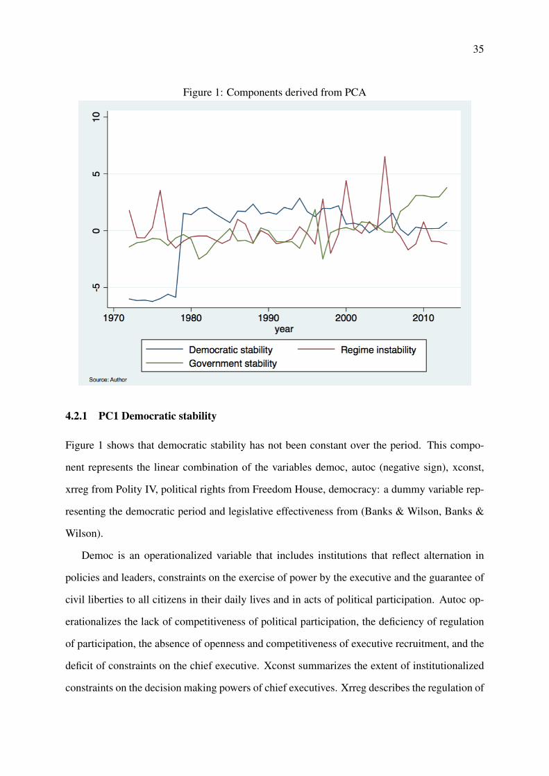
Figure 1: Components derived from PCA
4.2.1 PC1 Democratic stability
Figure 1 shows that democratic stability has not been constant over the period. This compo-
nent represents the linear combination of the variables democ, autoc (negative sign), xconst,
xrreg from Polity IV, political rights from Freedom House, democracy: a dummy variable rep-
resenting the democratic period and legislative effectiveness from (Banks & Wilson, Banks &
Wilson).
Democ is an operationalized variable that includes institutions that reflect alternation in
policies and leaders, constraints on the exercise of power by the executive and the guarantee of
civil liberties to all citizens in their daily lives and in acts of political participation. Autoc op-
erationalizes the lack of competitiveness of political participation, the deficiency of regulation
of participation, the absence of openness and competitiveness of executive recruitment, and the
deficit of constraints on the chief executive. Xconst summarizes the extent of institutionalized
constraints on the decision making powers of chief executives. Xrreg describes the regulation of

36
Chief Executive and is classified in three categories: unregulated, designational/transitional and
regulated. Unregulated alludes to changes in chief executive occur through forceful seizures
of power. Designational/transitional occurs when chief executives are chosen by designation
within the political elite, without formal competition. Regulated is presented when chief exec-
utives are determined by hereditary succession or in competitive elections (Gurr & Marshall.,
2013). Political rights from Freedom House alludes to the rights that enable people to partici-
pate freely in the political process, including the right to vote freely for distinct alternatives in
legitimate elections, compete for public office, join political parties and organizations, and elect
representatives who have a decisive impact on public policies and are accountable to the elec-
torate (FreedomHouse, 2016). Legislative effectiveness is encoded into four different options:
none, ineffective, partially effective and effective. There is none legislative effectiveness when
no legislature exists. Ineffective legislative occurs when activity may be of a ”rubber stamp”
character; domestic turmoil may make implementation of legislation impossible and effective
executive may prevent the legislature from meeting. Partially effective alludes to a situation in
which the effective executive’s power substantially outweighs, but does not completely dom-
inate, that of the legislature, Effective represents the possession of significant governmental
autonomy by the legislature (Banks & Wilson, Banks & Wilson).
Figure1 shows a structural break in 1979, when Ecuador returned to democracy, being this
the turning point from which most values become positive. Hence, high scores of the demo-
cratic stability index mean correspond to more democratic traits. Additionally, the figure shows
how democracy has deteriorated over time, specifically since 1999 and even more since 2007,
however it presents a slight improvement since 2012. This is due to the low scores of political
rights protection presented in the last decade, and the larger influence of the Executive. While
this component presents variation over the years, it is clear that there is a negative trend since
1994.
4.2.2 PC2 Regime instability
The second component represents regime stability. The major loadings are government crises,
purges, revolutions, and realized coups from (Banks & Wilson, Banks & Wilson). Govern-

37
ment crisis describes any rapidly developing situation that threatens to bring the downfall of
the present regime, excluding situations of revolt aimed at such overthrow. Purges refers to
any systematic elimination by jailing or execution of political opposition within the ranks of
the regime or the opposition. Revolutions operationalizes any illegal or forced change in the
top government elite, any attempt at such a change, or any successful or unsuccessful armed
rebellion whose aim is independence from the central government (Banks & Wilson, Banks &
Wilson). Hence, as presented in Figure 1 the highest points correspond to years in which a coup
d’etat occurred (1997, 2000 and 2005). Yet, there is also variation originated from the other
variables. For example, the series presents a peak in 2010 that corresponds to the 30S event,
when members of the national police upraised against the government. In this sense, this com-
ponent represents regime instability since it includes variables that threaten the constitutional
order. It not only incorporates government crisis, but coups d’etat that are a threat to the regime
in general. Therefore, higher values of this component represent a rise in the propensity of the
regime to collapse. Figure 1 confirms the lack of regime stability that was described in the
second section.
4.2.3 PC3 Government stability
The third component has as its major loadings years in office, general strikes with negative
sign, size of cabinet and number of seats of the largest party in the legislative from (Banks &
Wilson, Banks & Wilson). General strikes refers to any strike of 1,000 or more industrial or
service workers that involves more than one employer and that is aimed at national government
policies or authority (Banks & Wilson, Banks & Wilson). Hence, it represents government
stability per se, since it encloses all the elements or characteristics a government can present
in order to stay in power. It encompasses not only the relationship between the Executive and
the Legislative which have been a source of political instability as explained in section III, but
also the capacity of the government to stay in power as measured by the size of the cabinet. As
shown in Figure 1, higher values of this component represent more stability. In contrast to the
regime instability component, this component increases since 2006. However, it also reinforces
the idea that during the 90’s and until 2006, Ecuador had high rates of government instability.

38
4.3 Specification of the Model
Taking into consideration that there are three main components from the PCA representing the
different dimensions of political instability, each of them was analyzed in a different model.
Several studies have used structural equations in order to estimate both political instability and
economic growth jointly due to the endogeneity between these variables (Alesina & Perotti,
1996; Chen & Feng, 1996; Svensson, 1998; Annett, 2000). Because of the challenges of iden-
tifying the structural equations of economic growth and political instability for Ecuador and to
avoid specification errorr we estimate a Vector Autoregressive Model (VAR) or a Vector Error
Correction (VECM) depending on the characteristics of each series as in Faust & Irons (1999).
The baseline of each model includes a proxy variable for political instability obtained from the
PCA, the log of real GDP, log of oil production and as an exogenous variable real oil prices.
4.3.1 Model 1- Democratic stability
After analyzing the endogenous variables log of GDP, log of oil production and democratic
stability (PC1), and as exogenous variable the lagged difference of oil prices it is evident that
all variables present unit roots (Appendix C). However, there is no cointegration between them
(Appendix D). Hence, in order to analyze the relationship between democratic stability and
economic growth the following VAR was used:
∆LGDPt = α0 +α1∆LGDPt−1
+β1∆PC1t−1 + γ1∆PROILt−1 +δ1∆Oilt−1 + ε1
∆PC1t = β0 +α2∆LGDPt−1
+β2∆PC1t−1 + γ2∆PROILt−1 +δ2∆Oilt−1 + ε2
∆PROILt = γ0 +α3∆LGDPt−1
+β3∆PC1t−1 + γ3∆PROILt−1 +δ3∆Oilt−1 + ε3

39
4.3.2 Results Model 1
Table 3: Estimation results : VAR Model 1
Variable Coefficient (Std. Err.)Equation 1 : ∆ LGDPt−1
∆ LGDPt−1 0.282 (0.131)**∆ PC1t−1 -0.003 (0.003)∆ PROILt−1 0.003 (0.020)∆ LDOILt−1 0.001 (0.000)***Intercept 0.024 (0.006)***
Equation 2 :∆ PC1t−1∆ LGDPt−1 12.064 (7.238)*∆ PC1t−1 -0.102 (0.153)∆ PROILt−1 -1.017 (1.109)LDOIL -0.011 (0.014)Intercept -0.207 (0.321)
Equation 3 : ∆ PROILt−1∆ LGDPt−1 -0.705 (0.696)∆ PC1t−1 -0.017 (0.015)∆ PROILt−1 -0.250 (0.107)**∆ LDOILt−1 0.001 (0.001)Intercept 0.063 (0.031)**
* Significance at the 10% confidence level**Significance at the 5% confidence level*** Significance at the 1% confidence levelNumber of obs=40
The VAR shows that the variables affecting economic growth in the case of Ecuador are
the lagged difference of oil prices and the lagged difference of the log of GDP. This finding
highlights the importance of oil in the Ecuadorian economy in the period analyzed. This re-
sult coincides with the analysis presented before, as in the empirical research of Andrango &
Grijalva (2016) and Borja (2014). Nevertheless, the democratic stability index does not affect
economic growth in the short run. This is consistent with the fact that during the two periods of
strongest economic growth in Ecuador the country was under a military dictatorship and under
Rafael Correa’s presidency, which has been accused of non-democratic practices.
However, lagged economic growth does affect democratic stability. Taking into consider-
ation that a greater value of democratic stability (PC1) means that Ecuador has improved its
democracy, then the lagged difference of economic growth contributes positively to the demo-

40
cratic stability in Ecuador. This finding provides evidence for Ecuador of Lipset’s theory of
modernization, which states that “the the more well-to-do a nation, the greater the chances that
it will sustain democracy” (Lipset, 1959).
Finally, only the lagged difference of oil production affects negatively oil production. This
result is intuitive since efforts to increase oil production materialize in a discrete way. For
instance, once a new pipeline is finished, production increases significantly, but following that
pipeline, production tends to vary marginally until there is a new large investment to boost it.
4.3.3 Model 2- Regime instability
In order to analyze the relationship between regime instability and economic growth, it is neces-
sary to test for stationary and cointegration. As shown in Appendix C and Appendix D, both oil
production, oil prices, and real GDP present unit roots. However, the regime instability index
(PC2) is stationary (Appendix D). For this reason, we cannot estimate a Vector Error Correction
Model (VECM) in which all variables need to have the same degree of integration. We run a
Vector Autoregressive Model (VAR) considering as endogenous variables the difference of log
of the GDP, the difference of oil production and the index of regime instability (PC2) in levels
and as exogenous variable the lagged difference of oil prices. The second model specification
is the following:
∆LGDPt = α0 +α1∆LGDPt−1
+β1PC2t−1 + γ1∆PROILt−1 +δ1∆Oilt−1 + ε1
PC2t = β0 +α2∆LGDPt−1
+β2PC2t−1 + γ2∆PROILt−1 +δ2∆Oilt−1 + ε2
∆PROILt = γ0 +α3∆LGDPt−1
+β3PC2t−1 + γ3∆PROILt−1 +δ3∆Oilt−1 + ε3

41
Table 4: Estimation results : VAR 1974-2013
Variable Coefficient (Std. Err.)Equation 1 : ∆ LGDPt−1
∆ LGDPt−1 0.276 (0.133)**PC2t−1 0.001 (0.002)∆ PROILt−1 0.002 (0.020)∆ LDOILt−1 0.001 (0.000)***Intercept 0.024 (0.006)
Equation 2 : PC2t−1∆ LGDPt−1 2.352 (9.556)PC2t−1 0.024 (0.159)∆ PROILt−1 0.133 (1.465)∆ LDOILt−1 -0.010 (0.019)Intercept -0.104 (0.423)
Equation 3 : ∆ PROILt−1∆ LGDPt−1 -0.705 (0.706)PC2t−1 -0.006 (0.012)∆ PROILt−1 -0.259 (0.108)**∆ LDOILt−1 0.001 (0.001)Intercept 0.061 (0.031)
* Significance at the 10% confidence level**Significance at the 5% confidence level*** Significance at the 1% confidence levelNumber of obs=40
42
4.3.4 Results Model 2
As presented in Table 4, the variables that affect economic growth are the lagged difference
of oil prices and the lagged difference of economic growth. There is no relationship between
regime instability (PC2) and economic growth in the short run. This supports Polga & Mejia
(2011) argument that only the coup d’etat against Jamil Mahuad had economic motivations.
Likewise, none of the other variables (oil production, oil prices) has an effect on regime
instability. This could be explained because regime instability is the maximum point in the
spectrum of political instability. Hence, economic growth, oil prices and production could be
the triggers for the first stage of riots or anti government demonstrations, but a regime collapse
occurs only after a series of factors accumulate as explained by (Basabe & Polga, 2017). Finally,
the change in oil production is affected negatively by the lagged difference of oil production as
in the previous model.
4.3.5 Model 3 - Government stability
After testing the series of government instability (PC3), economic growth and oil production, all
of them present unit roots (Appendix C), the lags needed are two and there exists a cointegration
of order 1 (Appendix D). Therefore, the right model to analyze the interactions among them
is a VECM. This model analyzes the relationship between time series that are not covariance
stationary, but are cointegrated. Hence, there is a linear combination of the series that is sta-
tionary or I(0), while each independent series is I(1). A VECM is a system of equations where
each variable is explained by its own lagged differences and the lagged differences of the other
endogenous variables, plus a lagged error-correction term. The error correction term represents
the long-run equilibrium relationship between the series, while the lagged differences represent
the short-run effects. The specification of the model is the following:

43
∆LGDPt = α0 +αLGDPθt−1 +α1∆LGDPt−1
+β1∆PC3t−1 + γ1∆PROILt−1 +δ1∆Oilt−1 + ε1
∆PC3t = β0 +βPC3θt−1 +α2∆LGDPt−1
+β2∆PC3t−1 + γ2∆PROILt−1 +δ2∆Oilt−1 + ε2
∆PROILt = γ0 + γPROILθt−1 +α3∆LGDPt−1
+β3∆PC3t−1 + γ3∆PROILt−1 +δ3∆Oilt−1 + ε3
This system of equations represents the dynamics between government instability, oil pro-
duction and economic growth, and the lagged change in real oil prices as an exogenous variable.
The speed of adjustment parameters αLGDP, βPC3 and γPROIL represent the short term deviation
from the long term cointegration relationship. The lagged differences of the explanatory vari-
ables represent the short-run causality on the left-hand side variables.
4.3.6 Results Model 3
The cointegrating equation presents the long term relationship between the non-stationary vari-
ables. The equation below presents the coefficients of this relationship with the standard errors
in parenthesis.
θ = LGDP−0.108PC3−0.630LPROIL−9.993
(0.10)∗∗∗(0.03)∗∗∗
This equation shows that there is a positive feedback from government stability and oil
production to economic growth. Specifically, the relationship suggests that in the long run gov-
ernment stability contributes 0.10 index points to GDP growth, while oil production contributes
0.63 points.
The VEC Model (Table 5) relating government stability, oil production and GDP growth

44
Table 5: Estimation results: VECM 1974-2013
Variable Coefficient (Std. Err.)Equation 1 :∆ LGDPt−1
ce1t−1 -0.136 (0.044)***∆ LGDPt−1 0.153 (0.136)∆ PC3t -0.009 (0.004)**∆ PROILt -0.032 (0.022)∆ LDOILt−1 0.001 (0.000)**Intercept 0.028 (0.006)
Equation 2 : ∆ PC3tce1t−1 5.458 (1.943)***
∆ LGDPt−1 4.756 (6.043)∆PC3t 0.038 (0.195)∆PROILt 1.794 (0.997)*∆ LDOILt−1 0.000 (0.012)Intercept -0.004 (0.264)
Equation 3 : ∆ PROILtce1t−1 0.616 (0.240)***
∆ LGDPt−1 -0.092 (0.747)∆ PC3t 0.050 (0.024)**∆ PROILt -0.104 (0.123)∆ LDOILt−1 0.002 (0.001)Intercept 0.039 (0.033)
* Significance at the 10% confidence level* Significance at the 5% confidence level**** Significance at the 1% confidence levelNumber of obs=40
as endogenous variables and as exogenous variable the lagged difference of oil prices, presents
a short-run Granger causality between the lagged change in government stability (PC3) and
the lagged change in oil prices towards real GDP growth. In this sense, taking into considera-
tion that higher values of the government stability index represent a more stable government,
this means that in the short run an increase in government stability in the last year will have
a negative impact in economic growth on the current year. Although this result might sound
counterintuitive, it represents Ecuador’s economic and political dynamics. Most of the presi-
dents faced a trade-off between governance through populist policies or political instability and
a healthy economy. As explained in section III, from Febres Cordero until Mahuad, most of
the Ecuadorian presidents employed adjustment policies at the beginning of their periods that
contributed to a sustainable economy in the long run. However, in the short run when they

45
faced anti-government demonstrations due to the policies adopted, they set back part or all of
the adjustment measures and applied economic populist policies in order to remain in power,
but which are detrimental to economic growth (Pachano, 2007; Freidenberg & Pachano, 2016).
In the long run –as shown by the cointegrating equation– the relationship between gov-
ernment stability and economic growth is positive. This is in line with the findings of several
authors (Barro, 1991; Perotti, 1996; Alesina et al., 1996; Chen & Feng, 1996; Asteriou & Price,
2000; Carmignani, 2001; Jong-A-Pin, 2009). Additionally, the speed of adjustment regarding
GDP is significant, negative and less than 1 as required. The other variable significant to GDP
growth is the lagged change in oil prices, as in the previous models.
In the short-run, the only variable significantly affecting government stability is the lagged
change in oil production. A positive change in a period before regarding oil production will
contribute to the stability of government in power. The mechanism through which this rela-
tionship operates is through oil revenues generated by oil production. As presented in section
III, most of the governments that have registered larger oil revenues have used these resources
to boost social spending and to provide other economic benefits to the population in order to
remain in power. Additionally, throughout Ecuador’s political history economic resources have
been used in exchange of political favors (Freidenberg & Pachano, 2016) in order to maintain
governability. Hence, the source of government stability has been oil production.
In the short run, economic growth does not affect government stability. This seems to be
the case in Ecuador because political instability originated in conflicts between the Legislative
and the Executive power do not respond to economic situations, but to political conflicts of
interests. This was the case during the presidencies of Hurtado, Febres Cordero, Borja, Duran
Ballen, Bucaram, and Gutierrez.
Finally, only the lagged change in government stability Granger causes an increase in oil
production. The reason is that a stable political environment leads to an increase in oil pro-
duction due to the reduction in uncertainty. This finding reinforces the findings of Alesina &
Perotti (1996), who conclude that the political uncertainty following political turmoil affects the
enforcement of property rights and repels investment.

46
5 Conclusions
After analyzing the three dimensions of political instability: democratic stability (PC1), regime
instability (PC2) and government stability (PC3), and their endogenous relationship with eco-
nomic growth, there is no evidence that democratic stability affects economic growth. However,
economic growth does affect democratic stability providing supporting evidence of Lipset’s the-
ory of modernization in the case of Ecuador. In the same way, when analyzing regime instability
(PC2) there is no evidence of a negative impact on economic growth in the short run.
The only political variable that presents an effect on economic growth both in the short run
and in the long run is government stability (PC3). In the short run it has a negative effective
since it captures the dynamics of backtracking from adjustment measures and the implementa-
tion of populist policies that are detrimental to economic growth. However, in the long run it
presents a positive relationship, as presented in the cointegration equation. More government
stability contribute to political certainty, stable institutions, therefore more confidence and more
investment that boosts economic growth. In the same way, government stability has a positive
effect in oil production. However, neither regime instability nor democratic stability affect oil
production.
As presented in section III and IV oil production affects government stability because oil
revenues provide available resources to use in social spending and maintain government’s pop-
ularity and state capacity.
The only variable in the three models that affects economic growth is oil, showing the rel-
evance of oil resources and specially the change in the oil price in the Ecuadorian economy.
Finally, in the three models, the lagged difference of oil production affects negatively oil pro-
duction. As explained before, this result is robust and appeared in the three models since efforts
to increase oil production materialize in a discrete way.
47
6 References
Aisen, A. & Veiga, F. (2011). How does political instability affect economic growth? IMF
Working Paper.
Alesina, A., Ozler, S., Roubini, N., & Swagel, P. (1996). Political instability and economic
growth. Journal of Economic Growth, 1, 189– 212.
Alesina, A. & Perotti, R. (1996). Income distribution, political instability and investment. Eu-
ropean Economic Review, 40, 1203– 1228.
Andrango, J. (2013). Asamblea utopica. Carta Economica, (5).
Andrango, J. & Grijalva, D. (2016). Human development, democracy, and economic growth:
a case study of ecuador.
Andrango, J., Grijalva, D., & Romero, P. (2016). Liberalism in ecuador: In search of a consti-
tution.
Annett, A. (2000). Social fractionalisation, political instability, and the size of government.
IMF Working Paper.
Asteriou, D. & Price, S. (2000). Political instability and economic growth: Uk time series
evidence. City University.
Banks, A. & Wilson, K. Cross-national time-series data archive.
Barro, R. J. (1991). Economic growth in a cross-section of countries. The Quarterly Journal of
Economics, 106, 407– 443.
Barro, R. J. & Lee, J. (1994). Sources of economic growth. Carnegie-Rochester Conference
Series on Public Policy.
Basabe, S. & Polga, J. (2017). Desempeno economico y movilizacion social como detonantes
de las caıdas presidenciales: propuesta teorica y aplicaciones al caso ecuatoriano. Perfiles
Latinoamericanos, 50.

48
BCE. Informacion economica.
Benhabib, J. & Spiegel, M. (1997). Growth and investment across countries: are primitives all
that matter. New York University and Federal Reserve Bank of San Francisco.
Borja, L. (2014). Sobre los determinantes del crecimiento de la economıa ecuatoriana.
CAIC. Deuda ecuatoriana con los organismos multilaterales, comision para la auditoria integral
del credito publico.
Campos, N. & Karanasos, M. (2007). Growth, volatility and political instability: * non-linear
time-series evidence for argentina, 1896–2000. William Davidson Institute.
Campos, N. F. & Nugent, J. B. (2002). Who is afraid of political instability? Journal of
Development Economics, 67, 157–172.
Carmignani, F. (2001). Theory and evidence on the political economy of growth. Universita‘
degli Studi di Milano-Bicocca . Working Paper 31.
Carmignani, F. (2003). Political instability, uncertainty and economics. Journal of Economic
Surveys, 17(1).
Chen, B. & Feng, Y. (1996). Some political determinants of economic growth: Theory and
empirical implications. European Journal of Political Economy, 12, 609–627.
Crain, M. & Tollison, R. (1993). Time inconsistency and fiscal policy: empirical analysis of
u.s. states, 1969– 89. Journal of Public Economics, 51, 153– 159.
Darby, J., Li, C.-W., & Muscatelli, V. (2000). Political uncertainty, public expenditure and
growth. Glasgow University,.
Espinosa, S. (2000). Presidentes del Ecuador. Vistazo.
Faust, J. & Irons, J. (1999). Money, politics and the post-war business cycle. Journal of
Monetary Economics, 43, 61 – 89.

49
Feng, Y. (1997). Democracy, political stability and economic growth. British Journal of Politi-
cal Science, 27.
FreedomHouse (2016). Freedom in the world comparative and historical data. Technical report,
Freedom House.
Freidenberg, F. & Pachano, S. (2016). El sistema polıtico ecuatoriano. FLACSO.
Gachet, I., Maldonado, D., Oliva, N., & Ramirez, J. (2011). Stylized facts of the ecuadorian
economy: The economic cicle 1965-2008. Banco Central del Ecuador, Centro de Estudios
Fiscales.
Grilli, V., M. D. & Tabellini, G. (1991). Political and monetary institutions and public policies
in the industrial countries. Economic Policy, 13, 341 –392.
Gurr, Robert, K. J. & Marshall., M. (2013). Polity IV Project: Political Regime Characteristics
and Transitions, 1800-2013. Center for Systemic Peace.
Haan, J. D., Sturm, J.-E., & Beekhuis, G. (1999). The weak government thesis: some new
evidence. Public Choice, 101, 163– 176.
Herrera, H., Ordonez, G., & Trebesch, C. (2015). Political booms, financial crises. University
of Pennsylvania School of Arts and Sciences.
Jong-A-Pin, R. (2009). On the measurement of political instability and its impact on economic
growth. European Journal of Political Economy, 25(15-29).
Legislativo, O. Informe de actividad legislativa.
Levine, R. & Renelt, D. (1992). A sensitivity analysis of cross-country growth regressions.
American Economic Review,, 82, 942– 963.
Lipset, S. M. (1959). Some social requisites of democracy: Economic development and political
legitimacy. The American Political Science Review, 53(1), 69–105.
Mauro, P. (1995). Corruption and growth. The Quarterly Journal of Economics, 110, 681– 712.

50
Mejıa Andres, P.-H. J. (2011). Coalition erosion and presidential instability in ecuador. Latin
American Politics and Society, 53(2), 87–111.
Pachano, S. (2007). La trama de Penelope. FLACSO.
Perotti, R. (1996). Growth, income distribution, and democracy: what the data say. Journal of
Economic Growth, 1, 149–187.
Polga, J. (2013). Ecuador: Estabilidad institucional y la consolidacion de poder de rafel correa.
Revista de Ciencia Polıtica, 33(1), 135–160.
Polga, J. & Mejia, A. (2011). Coalition erosion and presidential instability in ecuador. Latin
American Politics and Society, 2(87-111).
Roubini, N. & Sachs, J. (1989). Government spending and budget deficits in the industrial
countries. Economic Policy, 8, 99 – 132.
Sala-i Martin, X. (1997). I just run four million regressions. NBER Working Paper.
Schuldt, J. (1994). ELECCIONES Y POLITICA ECONOMICA EN EL ECUADOR 1983-1994
Elecciones y Polıtica Economica en Ecuador. ILDIS.
Svensson, J. (1998). Investment, property rights, political instability: theory and evidence.
European Economic Review, 42, 1317– 1341.
Universo, E. Informes policiales y militar no cuentan misma historia del 30-s.

51
Appendix A
Variables description
Table 6: Variables description
Variables Description Source
Democ
Democracy contains three interdependent elements.
One is the presence of institutions and procedures
through which citizens can express effective
preferences about alternative policies and leaders.
Second is the existence of institutionalized
constraints on the exercise of power by the executive.
Third is the guarantee of civil liberties to all
citizens in their daily lives and in acts of
political participation.
Gurr, Jaggers &
Marshall 2013
Autoc
Autocracy operationalization includes:
competitiveness of political participation,
the regulation of participation, the openness
and competitiveness of executive recruitment,
and constraints on the chief executive.
Gurr, Jaggers &
Marshall 2013
Durable
The number of years since the most recent
regime change (defined by a three-
point change in the POLITY score over
a period of three years or less) or the end
of transition period defined by the lack
of stable political institutions (denoted
by a standardized authority score).
Gurr, Jaggers &
Marshall 2013

52
Xrreg
Regulation of Chief Executive is classified
in three categories encode:Unregulated: Changes
in chief executive occur through forceful seizures
of power. Designational/Transitional: Chief
executives are chosen by designation within the
political elite, without formal competition.
Regulated: Chief executives are determined by
hereditary succession or in competitive
elections.
Gurr, Jaggers &
Marshall 2013
Xconst
This variable refers to the extent of
institutionalized constraints on the
decision-making powers of chief executives,
whether individuals or collectivities
Gurr, Jaggers &
Marshall 2013
Freedom House
Political rights
Political rights enable people to participate
freely in the political process, including the
right to vote freely for distinct alternatives in
legitimate elections, compete for public office,
join political parties and organizations, and
elect representatives who have a decisive
impact on public policies and are accountable
to the electorate.
Freedom House
2015
Freedom House
Civil rights
Civil liberties allow for the freedoms of
expression and belief, associational and
organizational rights, rule of law, and
personal autonomy without interference
from the state.
Freedom House
2015

53
Assassinations
Any politically motivated murder or
attempted murder of a high government
official or politician.
Banks 2016
General Strikes
Any strike of 1,000 or more industrial
or service workers that involves
more than one employer and that is
aimed at national government policies or
authority
Banks 2016
Major
Government Crises
Any rapidly developing situation
that threatens to bring the downfall
of the present regime - excluding
situations of revolt
aimed at such overthrow.
Banks 2016
Purges
Any systematic elimination by
jailing or execution of political
opposition within the ranks of the
regime or the opposition
Banks 2016
Riots
Any violent demonstration or clash
of more than 100 citizens involving
the use of physical force
Banks 2016
Revolutions
Any illegal or forced change
in the top government elite,
any attempt at such a change,
or any successful or unsuccessful
armed rebellion whose aim is
independence from the central government
Banks 2016

54
Anti-government
Demonstrations
Any peaceful public gathering of at least
100 people for the primary purpose of
displaying or voicing their opposition to
government policies or authority,
excluding demonstrations of a distinctly
anti-foreign nature.
Banks 2016
Size
of Cabinet
Refers to the number of ministers of ”cabinet
rank”, excluding,undersecretaries,
parliamentary secretaries, ministerial alternates,
etc. Includes the president and vice-president
under a presidential,system, but not under
a parliamentary system
Banks 2016
Major
Cabinet Changes
The number of time in a year that a new
premier is named and/or 50%,of the cabinet
posts are assumed by new ministers.
Banks 2016
Changes
in Effective Executive
The number of times in a year that effective
control of executive power,changes hands.
Such a change requires that the new executive
be independent of his predecessor
Banks 2016
Number of Seats
of the Largest Party
Contains the number of seats held by
the largest party in the lower house
of each country’s national assembly.
Banks 2016
Size of Legislature
Lower House
Contains the total number of seats in
the lower houseBanks 2016
Coups
d’Etat
The number of extra constitutional or forced
changes in the top government,elite and/or its effective
control of the nation’s power structure in a given year.
Banks 2016

55
Legislative
EffectivenessLegislative Effectiveness Banks 2016
Constitutions Dummy if a new constitutions is drafted Author
Years in office Years in office of an elected president Author

56
Appendix B
PCA- Components Selection
Figure 2: PCA scree plot test

57
Appendix C
Unit root tests
Table 7: Unit root testsAugmentedDickey FullerTest
Philips-PerronTest
LevelLGDP -1.418 -0.640LPROIL 0.747 -0.925OIL -1.795 -6.765PC1 -2.348 -6.165PC2 -6.239*** -39.089***PC3 -1.759 -5.355First DifferenceD.LGDP -4.730*** -32.337***D.LPROIL -13.491*** -49.506***D.OIL -6.274*** -37.268***D.PC1 -6.826*** -44.668***D.PC3 -8.614*** -44.008***
* Significance at the 10% confidence level* Significance at the 5% confidence level**** Significance at the 1% confidence levelNumber of obs=40

58
Appendix D
Cointegration tests
Table 8: Cointegration test Model 1Cointegration test Model 1 (LGDP, PC1, LPROIL)
Johansen tests for cointegrationTrend= constantLags=2Number of obs=40Sample=Sample:1974 - 2013Maximumrank Parms LL Eigenvalue Trace
statistic5%critical value
0 15 -398.52636 . 21.6949* 29.681 20 -392.62355 0.25557 9.8893 15.412 23 -387.69345 0.21847 0.0291 3.763 24 -387.67889 0.00073
Table 9: Cointegration test Model 3Cointegration test Model 3 (LGDP, PC3, LPROIL)
Johansen tests for cointegrationTrend= constantLags=2Number of obs=40Sample=Sample:1974 - 2013Maximumrank Parms LL Eigenvalue Trace
statistic5%critical value
0 15 -389.91751 . 51.5277 29.681 20 -367.39282 0.67575 6.4783* 15.412 23 -364.15368 0.14952 0.0000 3.763 24 -364.15368 0.00000

59
Appendix E
Post estimation tests
E.1 Model 1
E.1.1 Residual Autocorrelation
Table 10: Residual Autocorrelation Model 1Residual Autocorrelation Test Model 1Lagrange Multiplier TestLag chi2 df Prob>21 13.1221 9 0.157162 5.4340 9 0.79495
The Lagrange Multiplier shows evidence that there is no residual autocorrelation.
E.1.2 Normally Distributed Disturbances
Table 11: Normally distributed disturbances testsJarque-Bera testEquation chi2 df Prob >chi2D LGDP 9.981 2 0.00680***D PC1 861.617 2 0.0000***D LPROIL 112.488 2 0.00000***ALL 984.086 6 0.00000***Skewness testEquation Skewness chi2 df Prob >chi2D LGDP -.79986 1.880 1 0.03890**D PC1 4.2056 6.389 1 0.00000***D LPROIL -1.5986 17.037 1 0.00003***ALL 139.21 3 0.00001***Kurtosis testEquation Kurtosis chi2 df Prob >chi2D LGDP 4.8518 0.593 1 0.44108D PC1 24.124 15.212 1 0.00010***D LPROIL 10.568 95.450 1 0.00000***ALL 844.870 3 0.00000***

60
The tests show that we reject the null hypothesis of error normality. However, this should
not create a problem because if the errors are not normally distributed but are independently
and identically distributed with zero mean and finite variance (which should be the case since
there is no evidence of autocorrelation), the estimates are still consistent but not effcient (Stata
Corp., 2013).
E.1.3 VAR Stability-Stationarity
Table 12: VAR Stability-StationarityVAR Stability-Stationarity
Eigenvalue Modulus-.3240231 .324023.1275536 +.1358998i .186383.1275536 -.1358998i .186383
As the 12 shows all the eigenvalues lie inside the unit circle, hence the VAR satisfies the
stability condition.
E.2 Model 2
E.2.1 Residual Autocorrelation
Table 13: Residual Autocrrelation Test Model 2Residual Autocrrelation Test Model 2Lagrange Multiplier TestLag chi2 df Prob>21 10.3992 9 0.319142 4.9642 9 0.83742
The Lagrange Multiplier shows evidence that there is no residual autocorrelation.
E.2.2 Normally distributed disturbances
The tests present evidence to reject the null hypothesis of error normality. However, as in
the previous model this should not create a problem because if the errors are not normally
distributed but are independently and identically distributed with zero mean and finite variance.

61
Table 14: Normally Distributed Disturbances TestsJarque-Bera testEquation chi2 df Prob >chi2D LGDP 3.951 2 0.13868PC2 81.802 2 0.0000***D LPROIL 112.335 2 0.00000***ALL 198.087 6 0.00000***Skewness testEquation Skewness chi2 df Prob >chi2D LGDP -.56394 2.120 1 0.14537PC2 2.2469 33.656 1 0.00000***D LPROIL -1.6674 18.534 1 0.00002***ALL 54.310 3 0.00001***Kurtosis testEquation Kurtosis chi2 df Prob >chi2D LGDP 4.0481 0.593 1 0.44108PC2 8.3747 15.212 1 0.00010***D LPROIL 10.502 93.801 1 0.00000***ALL 143.777 3 0.00000***
E.2.3 VAR Stability-Stationarity
Table 15: VAR Stability-StationarityVAR Stability-StationarityEigenvalue Modulus.2828675 .282868-.2538009 .253801.01217472 .012175
All the eigenvalues lie inside the unit circle, hence the VAR satisfies the stability condition.
E.3 Model 3
E.3.1 Residual Autocorrelation
The Lagrange Multiplier shows evidence that there is no residual autocorrelation.

62
Table 16: Residual Autocrrelation Test Model 3Residual Autocrrelation Test Model 3Lagrange Multiplier TestLag chi2 df Prob>21 12.7249 9 0.175452 6.7590 9 0.66220
E.3.2 Normally distributed disturbances
The tests present evidence to reject the null hypothesis of error normality. However, as in
the previous model this should not create a problem because if the errors are not normally
distributed but are independently and identically distributed with zero mean and finite variance.
Table 17: Normally distributed disturbances testsJarque-Bera testEquation chi2 df Prob >chi2D LGDP 1.712 2 0.42488D PC3 10.543 2 0.00514***D LPROIL 18.652 2 0.00009***ALL 30.907 6 0.00003***Skewness testEquation Skewness chi2 df Prob >chi2D LGDP -.2916 0.567 1 0.45150D PC3 -.73888 3.640 1 0.05642*D LPROIL -1.1318 8.541 1 0.00347***ALL 12.747 3 0.00522***Kurtosis testEquation Kurtosis chi2 df Prob >chi2D LGDP 3.8289 1.145 1 0.28459D PC3 5.0352 15.212 1 0.00860***D LPROIL 5.4631 95.450 1 0.00147***ALL 844.870 3 0.00041***
E.3.3 VECM Stability-Stationarity
The test shows that the VECM specification imposes 2 unit root. This could represent a problem
in the estimated model since the cointegration equation is not stationary.

63
Table 18: VECM Stability-StationarityEigenvalue Modulus3.368324 3.368321.147447 1.147451 11 1.3309601 .33096-.1445431 .144543