UNIVERSIDADE DE SÃO PAULO ESCOLA DE … · FERNANDO MASSAMI SATO Numerical experiments with stable versions of the Generalized Finite Element Method CORRECTED VERSION (Original version

UNIVERSIDADE DE SÃO PAULO

ESCOLA DE ENGENHARIA DE SÃO CARLOS

DEPARTAMENTO DE ENGENHARIA DE ESTRUTURAS

Fernando Massami Sato

Numerical experiments with stable versions of the Generalized Finite Element Method

São Carlos

2017

FERNANDO MASSAMI SATO

Numerical experiments with stable versions of the Generalized Finite Element Method

CORRECTED VERSION

(Original version is available at EESC-USP)

São Carlos

2017

Dissertation presented to the São Carlos

School of Engineering of the University

of São Paulo for obtaining the Master

degree in Science.

Advisor: Sergio Persival Baroncini

Proença

5

ACKNOWLEDGMENTS

To my advisor, Sergio Proença, for the guidance, patience and friendship during the graduation

and master degree research.

To my parents Mauricio and Mary, and my brothers Bruno and Eduardo for the support over the

years.

To my grandparents Taro and Kaoru for taking care of me during my childhood.

To my colleagues Dorival and Ayrton for the help during the meetings and programming tips.

To Professor Rodrigo Paccola and Ricardo Angélico for the contributions in my qualification exam.

To CAPES for the financial support.

ABSTRACT

SATO, F. M. Numerical experiments with stable versions of the Generalized Finite Element

Method. 2017. 97p. Dissertation (Master degree). São Carlos School of Engineering, University

of São Paulo, São Carlos, 2017

The Generalized Finite Element Method (GFEM) is essentially a partition of unity based method

(PUM) that explores the Partition of Unity (PoU) concept to match a set of functions chosen to

efficiently approximate the solution locally. Despite its well-known advantages, the method may

present some drawbacks. For instance, increasing the approximation space through enrichment

functions may introduce linear dependences in the solving system of equations, as well as the

appearance of blending elements. To address the drawbacks pointed out above, some improved

versions of the GFEM were developed. The Stable GFEM (SGFEM) is a first version hereby

considered in which the GFEM enrichment functions are modified. The Higher Order SGFEM

proposes an additional modification for generating the shape functions attached to the enriched

patch. This research aims to present and numerically test these new versions recently proposed for

the GFEM. In addition to highlighting its main features, some aspects about the numerical

integration when using the higher order SGFEM, in particular are also addressed. Hence, a splitting

rule of the quadrilateral element area, guided by the PoU definition itself is described in detail. The

examples chosen for the numerical experiments consist of 2-D panels that present favorable

geometries to explore the advantages of each method. Essentially, singular functions with good

properties to approximate the solution near corner points and polynomial functions for

approximating smooth solutions are examined. Moreover, a comparison among the conventional

FEM and the methods herein described is made taking into consideration the scaled condition

number and rates of convergence of the relative errors on displacements. Finally, the numerical

experiments show that the Higher Order SGFEM is the more robust and reliable among the versions

of the GFEM tested.

Keywords: Generalized Finite Element Method. Stable Generalized Finite Element Method.

Higher Order Stable Generalized Finite Element Method. Rate of convergence. Scaled condition

number.

RESUMO

SATO, F. M. Experimentos numéricos com versões estáveis do Método dos Elementos Finitos

Generalizados. 2017. 97p. Dissertação (Mestrado). Escola de Engenharia de São Carlos,

Universidade de São Paulo, São Carlos, 2017

O Método dos Elementos Finitos Generalizados (MEFG) é essencialmente baseado no método da

partição da unidade, que explora o conceito de partição da unidade para compatibilizar um conjunto

de funções escolhidas para localmente aproximar de forma eficiente a solução. Apesar de suas

vantagens bem conhecidas, o método pode apresentar algumas desvantagens. Por exemplo, o

aumento do espaço de aproximação por meio das funções de enriquecimento pode introduzir

dependências lineares no sistema de equações resolvente, assim como o aparecimento de elementos

de mistura. Para contornar as desvantagens apontadas acima, algumas versões aprimoradas do

MEFG foram desenvolvidas. O MEFG Estável é uma primeira versão aqui considerada na qual as

funções de enriquecimento do MEFG são modificadas. O MEFG Estável de ordem superior propõe

uma modificação adicional para a geração das funções de forma atreladas ao espaço enriquecido.

Esta pesquisa visa apresentar e testar numericamente essas novas versões do MEFG recentemente

propostas. Além de destacar suas principais características, alguns aspectos sobre a integração

numérica quando usado o MEFG Estável de ordem superior, em particular, são também abordados.

Por exemplo, detalha-se uma regra de divisão da área do elemento quadrilateral, guiada pela própria

definição de sua partição da unidade. Os exemplos escolhidos para os experimentos numéricos

consistem em chapas com geometrias favoráveis para explorar as vantagens de cada método.

Essencialmente, examinam-se funções singulares com boas propriedades de aproximar a solução

nas vizinhanças de vértices de cantos, bem como funções polinomiais para aproximar soluções

suaves. Ademais, uma comparação entre o MEF convencional e os métodos aqui descritos é feita

levando-se em consideração o número de condição do sistema escalonado e as razões de

convergência do erro relativo em deslocamento. Finalmente, os experimentos numéricos mostram

que o MEFG Estável de ordem superior é a mais robusta e confiável entre as versões do MEFG

testadas.

Palavras-chave: Método dos Elementos Finitos Generalizados. Método dos Elementos Finitos

Generalizados Estável. Método dos Elementos Finitos Generalizados Estável de ordem superior.

Razão de convergência. Número de condição escalonado.

LIST OF FIGURES

Figure 1 – (a) Representation of the pyramid or hat basis function i for a patch formed by

quadrilateral elements and vertex iV . (b) Master element. ......................................................... 30

Figure 2 – Example of an independent geometry domain mesh. (a) The approximation mesh that

contains the integration mesh. (b) The integration mesh. (c) and (d) details of the integration

mesh. ........................................................................................................................................ 31

Figure 3 – Type of mesh used in this research ........................................................................... 32

Figure 4 – Construction of the shape function of GFEM using as enrichment (a) polynomial (b)

non-polynomial functions. Where is the hat partition of unity,

jL

the enrichment function and

j

the shape function of GFEM. ............................................................................................... 33

Figure 5 – Element type classification ....................................................................................... 35

Figure 6 – Construction of SGFEM shape function ................................................................... 40

Figure 7 – Representation of flat-top partition of unity. (a) 1-D function for the left node, (b) 1-D

function for the right node ......................................................................................................... 43

Figure 8 – Quadrilateral element ............................................................................................... 43

Figure 9 – Representation of flat-top PoU 2D version ............................................................... 45

Figure 10 – Illustration of flat-top PoU with 1.0 and three integration points (black dots in the

figure) ....................................................................................................................................... 46

Figure 11 – Split in subdomains for flat-top PoU....................................................................... 47

Figure 12 – Example of a problem containing a reentrant corner. .............................................. 50

Figure 13 – Illustration of Equation (16) for 1 Γ and 2Γ both Dirichlet boundaries. (a) k = 1. (b)

k = 2. (c) k = 3. ......................................................................................................................... 51

Figure 14 – L-shaped panel ....................................................................................................... 54

Figure 15 – L-shaped panel: h-convergence for different values of ........................................ 56

Figure 16 – L-shaped panel: scaled condition number for analysis ......................................... 56

Figure 17 – L-shaped panel: h-convergence for incomplete polynomial .................................... 58

Figure 18 – L-shaped panel: scaled condition number for incomplete polynomial ..................... 59

Figure 19– L-shaped panel: h-convergence for complete polynomial ........................................ 60

Figure 20 – L-shaped panel: layer representation (a) Layer 0, (b) Layer 1 and (c) Layer 2. The red

dots highlight the enriched nodes .............................................................................................. 61

Figure 21 – L-shaped panel: h-convergence for singular layer 0 with different values of singularn

................................................................................................................................................. 62

Figure 22 – L-shaped panel: h-convergence for singular layer 1 with different values ofsingularn 62


................................................................................................................................................. 62

Figure 24 – L-shaped panel: comparison between methods with respect to h-convergence for

singular layer 0 ......................................................................................................................... 63


singular layer 1 ......................................................................................................................... 64


singular layer 2 ......................................................................................................................... 64

Figure 27 – L-shaped panel: comparison for incomplete polynomial and singular layer 0 .......... 65



Figure 30 – L-shaped panel: SCN for incomplete polynomial and singular layer 0 .................... 67



Figure 33 – L-shaped panel: h-convergence for complete polynomial and singular layer 2 ........ 68

Figure 34 – L-shaped panel: effect of mesh refinement ............................................................. 69

Figure 35 – L-shaped panel: nodal stress Sxy for mesh 64 x 32 using different enrichment ....... 70

Figure 36 – Edge cracked panel ................................................................................................. 70

Figure 37 – Edge cracked panel: h-convergence for different values of .................................. 72

Figure 38 – Edge cracked panel: SCN for analysis ................................................................. 72

Figure 39 – Edge cracked panel: relative error values for incomplete polynomial and mesh

refinement ................................................................................................................................. 74

Figure 40 – Edge cracked panel: scaled condition number for incomplete polynomial and mesh

refinement ................................................................................................................................. 74

Figure 41– Edge cracked panel: relative error values for complete polynomial and mesh

refinement ................................................................................................................................. 75

Figure 42 – Edge cracked panel: (a) Layer 0, (b) Layer 1 and (c) Layer 2. The red dots are the

enriched nodes .......................................................................................................................... 75

Figure 43 – Edge cracked panel: h-convergence for singular layer 0 with nsingular varying from 1

to 3 ........................................................................................................................................... 76


to 3 ........................................................................................................................................... 76


to 3 ........................................................................................................................................... 77

Figure 46 – Edge cracked panel: comparison between methods with respect to h-convergence for

singular layer 0 ......................................................................................................................... 78


singular layer 1 ......................................................................................................................... 78


singular layer 2 ......................................................................................................................... 79

Figure 49 – Edge cracked panel: h-convergence curves for incomplete polynomial and singular

layer 0 ....................................................................................................................................... 79


layer 1 ....................................................................................................................................... 80


layer 2 ....................................................................................................................................... 80

Figure 52 – Edge cracked panel: SCN for incomplete polynomial and singular layer 0 .............. 81



Figure 55 – Edge cracked panel: h-convergence for complete polynomial and singular layer 2 . 83

Figure 56 – Edge cracked panel: effect of mesh refinement ....................................................... 84

Figure 57 – Edge cracked panel: nodal stress Syy for mesh 64 x 64 for different enrichments ... 85

Figure 58 – Irregular polygonal panel........................................................................................ 85

Figure 59 – Irregular polygonal panel: subdivision in areas and singular point .......................... 86

Figure 60 – Irregular polygonal panel: h-convergence for incomplete polynomial and singular

layer 0 ....................................................................................................................................... 88

Figure 61 – Irregular polygonal panel: h-convergence for incomplete polynomial and singular

layer 1 ....................................................................................................................................... 88

Figure 62 – Irregular polygonal panel: SCN for incomplete polynomial and singular layer 0 ..... 89

Figure 63 – Irregular polygonal panel: h-convergence for complete polynomial and singular layer

1 ............................................................................................................................................... 89

Figure 64 – Irregular polygonal panel: Effect of mesh refinement. ............................................ 91

LIST OF TABLE

Table 1 – First derivative for the singular function .................................................................... 51

Table 2 – L-shaped panel: relative errors for incomplete polynomial ......................................... 57

Table 3 – L-shaped panel: degrees of freedom for incomplete polynomial ................................. 58

Table 4 – L-shaped panel: scaled condition number for complete polynomial ........................... 59

Table 5 – L-shaped panel: SCN for complete polynomial and singular layer 2 .......................... 68

Table 6 – Edge cracked panel: Relative errors for incomplete polynomial enrichment ............... 73

Table 7 – Edge cracked panel: scaled condition number for complete polynomial ..................... 75

Table 8 – Edge crack panel: SCN for complete polynomial and singular layer 2 ....................... 82

Table 9 – parameter and singular function for each corner ...................................................... 87

Table 10 – Irregular polygonal: SCN for complete polynomial and singular layer 1 .................. 90

LIST OF ABBREVIATIONS

C-XFEM Corrected eXtended Finite Element Method

DoF Degrees of Freedom

FEM Finite Element Method

GFEM Generalized Finite Element Method

PoU Partition of Unity

PUM Partition of Unity Method

SCIEnCE São Carlos Integrity Environment for Computational Engineering

SCN Scaled Condition Number

SGFEM Stable Generalized Finite Element Method

LIST OF SYMBOLS

j

Shape function

Partition of unity

jL

Enrichment function

u Conventional degree of freedom

ju

Additional nodal parameter

j (mod)L Modified enrichment function

I Interpolant function of nodal values

j (mod)

Modified shape function

FEMS Standard FEM approximation space

mod

enrichS Augmented space related to the modified enrichment functions

FT

Flat-top partition of unity

Parameter for controlling the flat region length that can vary between 0.0

and 0.5

Angle for the singular function measured internally to the solid

singularn Number of terms optionally adopted for singular function

CONTENTS

1 Introduction ....................................................................................................................... 25

1.1 Objectives ................................................................................................................... 27

1.2 Materials and methods ................................................................................................ 27

1.3 Structure of the dissertation ......................................................................................... 28

2 The Generalized Finite Element Method ............................................................................ 29

2.1 A brief historical review.............................................................................................. 29

2.2 Formulation ................................................................................................................ 32

2.3 Some general comments on the Blending Elements ..................................................... 35

2.4 On the conditioning of the underlying linear system .................................................... 36

3 The Stable Generalized Finite Element Method.................................................................. 39

4 The Higher Order SGFEM ................................................................................................. 41

5 numerical integration and split strategy for higher order sgfem .......................................... 47

6 The enrichment functions ................................................................................................... 49

6.1 Singular function ........................................................................................................ 49

6.2 Polynomial functions .................................................................................................. 52

7 Numerical examples and discussion ................................................................................... 53

7.1 L-shaped panel ............................................................................................................ 53

7.1.1 Parameter analysis........................................................................................... 55

7.1.2 Polynomial enrichment ........................................................................................ 57

7.1.3 Singular enrichment ............................................................................................. 60

7.1.4 Polynomial and singular enrichment combined .................................................... 64

7.2 Panel presenting an edge crack .................................................................................... 70

7.2.1 Parameter analysis........................................................................................... 71

7.2.2 Polynomial enrichment ........................................................................................ 73

7.2.3 Singular enrichment ............................................................................................. 75

7.2.4 Polynomial and singular enrichment combined .................................................... 79

7.3 Panel with multiple corners, polygonal voids and edge cracks ..................................... 85

8 Conclusion ......................................................................................................................... 93

References ................................................................................................................................ 95

25

1 INTRODUCTION

The Finite Element Method (FEM) is indeed one of the most powerful tools of computational

engineering. However, this method has shown to be ineffective or having limited efficacy when

used to simulate problems presenting some special features, such as solids containing reentrant

corners, cracks, materials interfaces and boundary layers. In fact, to account for these kinds of

features, an exaggerated mesh refinement is normally required around these singularity regions.

Therefore, using conventional FEM, obtaining satisfactory numerical results demands higher

computational costs.

The Generalized Finite Element Method (GFEM), Strouboulis, Babuška and Copps (2000), was

proposed both to address the mesh refinement problem and efficiently solve the above mentioned

classes of special problems, therefore overcoming some of the inconveniences presented by the

FEM.

The GFEM is essentially a partition of unity based method (PUM) that explores the Partition of

Unity (PoU) concept to match a set of functions chosen to efficiently approximate the solution

locally. These local approximations are called enrichment functions and once matched increase the

global conforming approximation space.

The GFEM contains the FEM shape functions in particular. However, differently from the standard

FEM, where the shape functions are attached to elements, in the GFEM the shape functions are

attached to a node. This node is vertex of a local patch, which is the region where the shape function

is defined. In the GFEM, overlapping patches covering the domain of the problem can be defined

with the help of a finite element mesh. A patch is then defined by the set of elements sharing a

common node, which is its vertex.

The main characteristic of the GFEM is the possibility to introduce an a priori knowledge into the

approximation about the solution through the enrichment functions. Moreover, according to the

peculiarities of the problem, the method enables the selective improvement of the approximation

space only where it is necessary. Consequently, a good global approximate solution can be obtained

even if using a coarse mesh, therefore reducing the computational cost.

26

Despite the above mentioned advantages, the method may present some drawbacks. For instance,

increasing the approximation space through enrichment functions may result in a system of

equations linearly dependent. In this case, round-off errors prevail when solving the system,

making the approximate solution less reliable. As will be shown later, the level of instability can

be assessed by the Scaled Condition Number (SCN). In the worst cases of instability, the SCN is

of a higher order of magnitude compared to the FEM level. Another drawback presented by the

GFEM derives from the so-called blending elements. This kind of element appears when the

enrichment is limited to a restricted region of the domain or number of patches. Then, looking at

the elements of a mesh, instead of the patches, it may happen that only some nodes are enriched or

that the nodes show a different number of enrichment functions. Consequently, unwanted

approximation terms appear, adversely influencing the rate of convergence of the global solution.

To address the drawbacks mentioned above, some improved versions of the GFEM were

developed, such as the Stable Generalized Finite Element Method (SGFEM), Babuška and

Banerjee (2012) and the Corrected eXtended Finite Element Method (C-XFEM), Fries (2008). In

this research, the C-XFEM will not be considered.

The SGFEM is a version of the GFEM where the enrichment functions are modified. In short, the

modified enrichment function is the enrichment function of the GFEM minus a linear or bilinear

interpolation of its nodal values. This version was proposed with the premise of solving two issues:

the linear dependency of the resulting system and the unwanted terms existing in the blending

elements.

Despite its premise, the SGFEM can still be ineffective for solving the problem of linear

dependences, as exemplified by the examples presented herein. In fact, when considering complete

second degree enrichment, for instance, the SCN is shown to be likewise bad, once presenting a

magnitude order comparable to the value obtained for GFEM. To deal with this issue, a new

improved 2-D GFEM version called Higher Order SGFEM, Zhang, Banerjee and Babuška (2014),

is also introduced and hereby tested.

The Higher Order SGFEM proposes a further modification for generating the shape functions

attached to the enriched patch. This improvement consists of using a flat-top PoU for multiplying

the local enrichment functions. Due to the particular features of the flat-top PoU, it is expected that

27

the resulting set of shape functions is linearly independent. In fact, the effectiveness of this

improved version of the GFEM is numerically demonstrated in the examples hereby presented.

1.1 Objectives

The main aim is to present and test some of the new developments recently proposed for the GFEM.

In particular, an improved formulation of the method called Stable GFEM, as well as its higher

order version are addressed through a numerical investigation.

As the main objective, the purpose of this research is to compare the above mentioned GFEM

versions with the conventional FEM. The focus is to identify the advantages and shortcomings of

each method, and to conclude if there is one among them which is more robust and reliable.

1.2 Materials and methods

The methodology adopted in this research consists firstly of a bibliographic review about the

GFEM and its improved versions, SGFEM and higher order SGFEM.

The second step comprises an investigation of the advantages and shortcomings of each method

through two-dimensional numerical examples. The analysis was conducted using the São Carlos

Integrity Environment for Computational Engineering (SCIEnCE) code, which has already had

these versions implemented.

Moreover, the analysis of the numerical results was then taken as a guideline for proceeding the

investigation. For instance, based on the results it was shown that when considering a complete

polynomial as enrichment, both GFEM and SGFEM reveal high scaled condition numbers,

therefore indicating ill-conditioning of the resulting system of equations. To overcome this

disadvantage, a 2-D version of the higher order SGFEM was implemented and tested.

Finally, a comparison between the methods herein described and the conventional FEM is made

through selected numerical examples. For instance, the rates of convergence for the relative errors

28

on displacements and the scaled condition number were used to highlight the overall GFEM

efficacy and also to identify which one among the GFEM versions is more robust and reliable.

1.3 Structure of the dissertation

Besides the Introduction section, this dissertation has seven more chapters. The outline of the

chapters is as follows:

In Chapter 2, a brief review of the GFEM is presented. However, some details are given regarding

the formulation, main advantages and drawbacks of the method. Moreover, the modified versions

developed to overcome the GFEM drawbacks are addressed.

Chapter 3 is related to the SGFEM. Essentially, the modification of the enrichment function, aiming

to overcome the GFEM problems is emphasized.

In Chapter 4, the Higher Order version of the SGFEM is presented. The main aspects related to the

flat-top PoU definition for 1-D and 2-D analysis using quadrilateral elements are discussed,

including some comments on the numerical integration.

Chapter 5 focuses on the numerical integration of the resulting 2-D enriched shape functions for

the Higher Order SGFEM. In particular, a splitting rule of the quadrilateral element area, guided

by the PoU definition itself is described in detail.

In Chapter 6, the enrichment functions considered in this research are presented. Essentially,

singular functions with good properties to approximate the solution near corner points and the

polynomial functions for approximating smooth solutions are examined.

In Chapter 7, three numerical examples are presented. The first one is an L-shaped panel, in which

the reentrant corner favors the use of a special enrichment. The second example is a panel

containing an edge crack. Again, enrichments with special and polynomial functions are explored.

The third example is an irregular polygonal panel containing multiple voids and reentrant corners,

as well as two edge cracks. In these examples, comparisons among the GFEM versions are made

in relation to the h-convergence rate and scaled condition number.

In Chapter8, the conclusions and final remarks are presented.

29

2 THE GENERALIZED FINITE ELEMENT METHOD

The generalized finite element method was developed to solve problems where the standard FEM

is inefficient or is costly computationally due to the extreme mesh refinement required, e.g.

problems involving stress concentrations induced by cracks and reentrant corners, boundary layers

and materials interfaces. The main idea of this method is to increase the FEM trial and test function

spaces with functions a priori in harmony with the solution.

2.1 A brief historical review

The GFEM can be seen as a version of Galerkin’s method, which is characterized by the availability

of more flexible approximations to the solutions of boundary value problems.

Historically, the conception of this method is preceded by the seminal proposal of Babuška and

Osborn (1983), according to which the shape of the approximation function is ruled by the

differential equation of its own problem. Next, Babuška, Caloz and Osborn (1994) proposed the

Special Finite Element Method. In this version, local approaches presenting characteristics of the

solution sought were incorporated into the approximation space using the Partition of Unity (PoU)

concept. Later, the idea of exploring the PoU for matching the local approximations and

constructing a global approximation was formalized in the Partition of Unity Method (PUM),

Melenk and Babuška (1996).

The PUM is a new finite element method that can create conform approximation spaces presenting

local features that are interesting for the solution. One of the main advantages of this method is that

an a priori knowledge of the solution can be incorporated into the approximation space. Moreover,

approximation spaces with any regularity can be easily constructed.

The construction of the approximation space of the PUM essentially explores the concepts of

Partition of Unity and covering sets called patches or clouds. Accordingly, the domain of the

given problem is covered by overlapping subdomains i . A set of enrichment functions associated

to each subdomain is then defined as: 1i i

i j j iL L L H , where H1 is the Hilbert space of

30

functions with continuous first order derivative. The global approximation to the solution can then

be defined as

i i

PUM i j j

i j

u u L

(1)

where ijL is the enrichment function, i

ju parameter involved in the linear combination of the

enrichment functions and the sequence of shape functions i are a partition of unity

0C which is

used to paste together the local enrichments, thus ensuring continuity for the global approximation.

In GFEM, the shape functions are defined in subdomains called patches. The concept of patches

was preceded by the concept of clouds introduced by Duarte (1996) in its proposition of the hp-

Cloud method. A patch in the GFEM is a subdomain created, for example, by quadrilateral

elements sharing a common node called vertex iV . In each patch, the functions i that appear in the

relation (1) show the unity value at the vertex of this subdomain and the null value on its boundary.

Moreover, as shown in Figure 1(a), the shape functions i are constructed by gathering the PoU of

each element i and attaching them to the vertex of the patch, defined as follows:

1 1

4

i k k

k

(2)

Figure 1 – (a) Representation of the pyramid or hat basis function i for a patch formed by quadrilateral elements

and vertex iV . (b) Master element.

Adapted: Strouboulis, Babuška and Copps (2000)

31

In the relation (2), the superscript i is for the element in the patch, k is the node number of the

element in coincidence with the vertex, while and are the coordinates of the master

quadrilateral element shown in Figure 1(b).

Finally, once the partition of unity ik merge, the resulting function i is piecewise bilinear. The

PoU generated by the overlapping of subdomains is 0C and will guarantee the inter-element

continuity and will create a 0C approximation.

As the main advantages of the GFEM, the following can be mentioned:

a) for each patch, a set of enrichment functions can be adopted presenting characteristics

of good local approximation for the solution;

b) through the concept of the augmented trial space of the FEM, a better approximated

solution can be obtained without the need of exploring a refined mesh;

c) there is a possibility of using meshes which are independent of the domain geometry,

as depicted in Figure 2, however by doing this two meshes need to be created. One

approximation mesh and an integration mesh, Figures 2(a) and 2(b), respectively.

Figure 2 – Example of an independent geometry domain mesh. (a) The approximation mesh that contains the

integration mesh. (b) The integration mesh. (c) and (d) details of the integration mesh.

Adapted: Strouboulis, Copps and Babuška (2001)

Despite the possibility of using a mesh independent of the domain, this research explores the

standard non-overlapping FEM meshes, e.g. the mesh is built by subdividing the domain into

32

triangular or quadrilateral elements satisfying the restrictions about the connections between the

neighbor elements, as shown in Figure 3.

Figure 3 – Type of mesh used in this research

Adapted: Strouboulis, Copps and Babuška (2001)

Therefore, considering a standard FEM mesh, as well as exploring the concepts of PUM and local

enrichments in the patches, the formulation of the GFEM is formally presented next.

2.2 Formulation

Despite exploring a mesh of elements, the shape functions of GFEM are conceptually different

from those of the conventional FEM, as their construction follows the PUM framework. In fact, in

the GFEM the shape functions are attached to patches , while in the FEM the shape functions

are defined in finite elements.

Therefore, the GFEM shape functions (j

) result from the multiplication among the linear or

bilinear partition of unity ( ) provided by triangular and quadrilateral elements, respectively, and

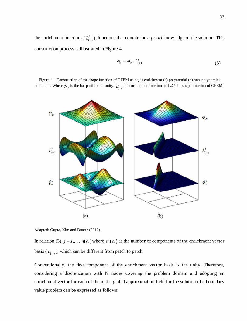
33

the enrichment functions ( jL

), functions that contain the a priori knowledge of the solution. This

construction process is illustrated in Figure 4.

j jL

(3)

Figure 4 – Construction of the shape function of GFEM using as enrichment (a) polynomial (b) non-polynomial

functions. Where is the hat partition of unity,

jL

the enrichment function and j

the shape function of GFEM.

Adapted: Gupta, Kim and Duarte (2012)

In relation (3), j 1, ,m where m is the number of components of the enrichment vector

basis ( L

), which can be different from patch to patch.

Conventionally, the first component of the enrichment vector basis is the unity. Therefore,

considering a discretization with N nodes covering the problem domain and adopting an

enrichment vector for each of them, the global approximation field for the solution of a boundary

value problem can be expressed as follows:

34

1 1

1 1 2

1 1

ˆ

ˆ

e

e

mNj j

h

j

mNNj j

j

NN

u u

x u x L x u

x u x L

(4a,b,c)

In the relation (4b), Ne ( N) is the number of enriched nodes. The first sum refers to an

approximation given by the PoU multiplied by the unity, i.e. this sum refers to the standard FEM

approximation, and involves conventional degrees of freedom ( u ) attached to the nodes of the

finite element. The second sum involves additional nodal parameters ju

, associated to the

remaining components of the enrichment vector basis. Moreover, the sum between brackets at

relation (4b) can be condensed into the parameter Lthat contains the enrichment functions and

the additional nodal parameters for each node α. The relation (4c) shows the role of the PoU for

matching the local approximations.

As already mentioned before, the enrichment functions provide local approximations. Moreover,

as exemplified in relation (4), the enrichment is not necessarily imposed for the whole set of nodes,

i.e., a number of nodes can remain having the unity as its single component in the enrichment

vector basis. This possibility of selective enrichment can be useful, for instance, in domains

presenting reentrant corners and/or cracks. In fact, in this kind of problem, the solution can be

smooth in most of the domain, however presenting some sort of singularity only in the

neighborhood of the crack or reentrant corner.

The local approximation provided by the method is a key advantage indeed, however there may be

drawbacks. When selective enrichment is adopted, at the element level, no enriched elements,

uniformly enriched elements or blending elements, in this case presenting different levels of

enrichment in their nodes, can appear. Consequently, the approximation of the blending element in

particular can be badly affected and special treatment is needed in these elements for recovering

its effectiveness.

35

2.3 Some general comments on the Blending Elements

Considering a given mesh, as a result of the selective local enrichment, the elements can be

collected in three distinctive categories. The first one includes the standard elements that do not

present enriched nodes. In the second category are the so-called reproducing elements that have all

the nodes with the same enrichment functions. The third one comprises the blending elements that

only have some of their nodes enriched or have different enrichments at the nodes. In the second

category, as a consequence of the PoU sum property equal to one, the enrichment function can be

reproduced precisely inside the elements. The lack of this favorable feature is the main drawback

of the blending elements. Therefore, in the last category, the enrichment functions cannot be

reproduced and depending on the type of function, the resulting local approximation can affect

directly both the quality of the global approximation and rate of convergence. The element

classification mentioned is illustrated in Figure 5.

Figure 5 – Element type classification

Adapted: Lins (2015)

Still regarding blending elements, according to Fries (2008) the issue requiring the most attention

is the introduction of unwanted terms in the approximation due to the difference among nodal

enrichments. The uneven or unwanted terms cannot be reproduced inside the element and impact

the convergence rate significantly. In the following example, a quadrilateral element containing

only one node enriched is considered:

2 2

1

ˆN

hu x u x L x u

(5)

36

where N is the number of nodes and is the enriched node. In general, the application of

enrichment functions produces unwanted terms that result from 2x L and its detrimental

influence cannot be compensated by the FEM part 1

ˆN

x u

. Therefore, the only way to not

generate unwanted terms is making 2 0u , which means that the enrichment is deactivated.

To overcome the drawbacks caused by the blending elements, some new versions of the GFEM

have been proposed. Some of them are briefly specified below:

a) Stable Generalized Finite Element Method (SGFEM): this method proposes a modification

in the enrichment functions that can reduce the deleterious influence of blending elements

on the rate of convergence, Babuška and Banerjee (2012);

b) Corrected eXtended Finite Element Method (C-XFEM): this method introduces a ramp

function on the blending elements to eliminate unwanted terms of approximation and to

recover the property of reproducibility of the enrichment, Fries (2008);

c) kC -GFEM: This method explores PoU with higher regularity build by the moving least

square technique, Torres, Barcellos and Mendonça (2015).

The SGFEM was chosen in this research for treating the blending elements because this method

was conceived to overcome not only the blending element effects, but also the additional drawback

associated to the ill-conditioning of the stiffness matrix.

2.4 On the conditioning of the underlying linear system

Essentially, the conditioning of a linear system of equations is related to how reliable the solution

will be.

Consider the linear system cAx . If the system is well-conditioned, it means that a small change

in the coefficient matrix A or a small change in vector c will result in a small change in the solution

vector x. On the other hand, if the system is ill-conditioned, a small change in matrix A or a small

change in vector c will result in a significant change in solution vector x.

37

The condition number is a scalar measure of the conditioning of a system and, therefore, indicates

the loss of accuracy of the computed solution. If the condition number is small then the system is

well conditioned, otherwise, it is ill conditioned. An ill-conditioned matrix includes linear

dependencies among its equations.

In the GFEM, as any function can be used as enrichment, the underlying linear system may not be

well conditioned with respect to the mesh and enrichment adopted. This shortcoming occurs when

functions presenting similar characteristics are adopted, such as PoU and enrichment. For instance,

when hat functions are adopted as PoU and polynomial are used for enrichment, the shape functions

may result almost linearly dependent and, therefore, the stiffness matrix is ill conditioned.

Regarding its measure, a condition number close to the value computed for the FEM is an

acceptable indicator of well conditioning of the GFEM underlying the linear system. Here, a further

improved measure called Scaled Condition Number (SCN) of the stiffness matrix will be used,

Babuška and Banerjee (2012). According to Zhang, Banerjee and Babuška (2014), given the

coefficient matrix A, this value can be obtained by computing the condition number 2 of the

scaled matrix Â based on 2

vector norm, as indicated below:

1

2 22 2

ˆ ˆ ˆk A : A DAD A A (6)

where D is a diagonal matrix having its diagonal terms computed as:21 iiii AD .

In this equation, the scaled matrix Â is obtained by pre and post multiplying the coefficient matrix

A by the diagonal matrix D. Moreover, the SCN can also be calculated by the ratio between the

largest and smallest eigenvalues of the scaled matrix.

A way to reduce the occurrence of linear dependencies in the GFEM is to use enrichment functions

that are of a different nature with respect to the PoU. In other words, if the PoU is polynomial, a

non-polynomial enrichment function should be used.

However, even if the dependencies are presented and consequently the SCN is large, it is possible

to solve a linear system where the stiffness matrix is semi-positive definite. It can be done by

making a scaling process on the stiffness matrix and after that, imposing a little perturbation in its

diagonal terms, as originally proposed by Strouboulis, Babuška and Copps (2000). It is important

38

to note that although the ill-conditioned system can deliver multiple solutions to the unknown

coefficients, the boundary value problem presents a unique solution.

The above mentioned procedure for solving the ill-conditioned system is iterative hence, depending

on the problem it can be computationally costly. Therefore, the SGFEM was conceived as a more

robust and general method to avoid the problem of the ill-conditioned stiffness matrix.

39

3 THE STABLE GENERALIZED FINITE ELEMENT METHOD

The so-called Stable Generalized Finite Element Method is a new version developed to overcome

two drawbacks observed in the GFEM. The method does not have the ill conditioning problem of

the stiffness matrix and significantly reduces the negative effects caused by blending elements,

Babuška and Banerjee (2012).

The basic difference between the stable and the conventional versions of the GFEM is a simple

modification in the enrichment functions used to obtain the shape functions. In SGFEM, the

enrichment function is modified in such a way that its values at the patch nodes are equal to zero.

The construction of this modified enrichment function j (mod)L is shown below:

j (mod) j jL L I L (7)

where jI L is the linear or bilinear piecewise interpolant of nodal values of the enrichment

function jL for the patch . Therefore,

I is:

1

,epN

j

i i i

i

I L x y

(8)

Where epN is the number of element nodes belonging to the patch, i is the node of the element in

analysis and ,i ix y is its coordinates.

Once the enrichment functions are modified, the SGFEM shape functions can be constructed

similarly to the GFEM:

j (mod) j (mod)L (9)

Figure 6 illustrates the construction of the SGFEM nodal shape function.

40

Figure 6 – Construction of SGFEM shape function

Adapted: Gupta et al. (2015)

As the vector of enrichment functions presents the unity as its first component, the approximation

space to the field of interest can be split as in GFEM:

mod

h FEM enrichu S S (10)

where FEMS is the standard FEM approximation space and modenrichS is the augmented space related to

the modified enrichment functions. Since the construction of the shape functions and therefore the

approximated field for SGFEM is the same as for GFEM, this method is easy to implement.

Concerning the issue of the blending elements, since the values of the SGFEM shape functions are

null at the element nodes, the effects of unwanted terms in the approximation are reduced.

Therefore, no special treatment in the blending elements is necessary.

As can be concluded from the procedure mentioned above, the modification of the enrichment

function basically eliminates the linear portion of it, therefore avoiding conflict with the linear

approximation ability already presented in the PoU. Consequently, the equations of the system are

expected to be better conditioned and the scaled condition number close to that obtained for FEM.

Even though such good features are actually verified in the 1-D approach, the scaled condition

number for SGFEM could still be large in the 2-D approach, as demonstrated by the examples

described herein. To overcome this problem, a further modification to the method can be

implemented leading to the higher order version of the Stable GFEM, hereby selected to be studied

and implemented in the SCIEnCE code.

41

4 THE HIGHER ORDER SGFEM

The higher order SGFEM, Zhang, Banerjee and Babuška (2014), was developed to yield higher

order convergence and to ensure good conditioning of the stiffness matrix in any dimensional

approach. This new version of the GFEM is derived from a further specific modification of the

enrichment space aiming to ensure that the shape functions of the enriched space are locally almost

linearly independent, while maintaining good flexibility for the construction of local

approximations as in the standard SGFEM.

Essentially, the suggested modification consists of using another PoU for constructing the mod

enrichS

space, different from the piecewise hat functions that however are preserved for constructing the

basic SFEM space. Thus, the higher order SGFEM approximation space is represented as follows:

mod

enrichFEMSGFEM SSS (11)

1

1

mod (mod)

1 2

Le

N

FEM

NNFT j j

enrich

j

S u

S L a

(12)

In the mod

enrichS space definition, mod

iL is constructed as indicated in relation (7), where LN is the

number of enrichment functions applied on node , while FT

represents the so-called ‘flat-top’

PoU function, Griebel and Schweitzer (2002). According to Zhang, Banerjee and Babuška (2014),

the use of another partition of unity to construct the modenrichS will contribute to generating linearly

independent enrichment spaces, and consequently, a good conditioning of the linear system will be

warranted.

42

1

1 ,

1 , 11 2

0 1 ,

j j

ll

jFT

Left j j

j j

x x x h

x x hx x x h x h

h

x x h x

(13)

1

0 ,

1 1 , 11 2

1 1 ,

j j

ll

jFT

Right j j

j j

x x x h

x x hx x x h x h

h

x x h x

(14)

The relations defining the flat-top PoU attached to a two node bar element and hereby adopted in

the 1-D approach are presented below. The relations above FT

Left x and FT

Right x are for the

functions attached to the left and to the right node, respectively, jx and

1jx are the nodal

coordinates, h is the element length, is a parameter for controlling the flat region length that can

vary between 0 and 0.5 and l is a positive integer for controlling the smoothness of the curve

segment linking the flat regions. Figure 7 (a) and (b) shows, respectively, the functions FT

Left x

and FT

Right x for a 1-D master element in correspondence to 2h , 0 25. and 1l .

43

Figure 7 – Representation of flat-top partition of unity. (a) 1-D function for the left node, (b) 1-D function for the

right node

The tensorial product of the 1-D functions described above is used for constructing the 2-D version

of the flat-top PoU associated to a regular quadrilateral element depicted in Figure 8.

Figure 8 – Quadrilateral element

The relations defining the component attached to node 1 are the following.

44

1

1

1 for

11 1 for

1 2 1 2

j jFT

j j

l ll l

j jj jFT

x x ,x h

y y , y h

x x h,x hx x h y y h

h h

1

1

1

1

1

1 0 for

0

j j

j jFT

j j

FT

y y h, y h

x x h, x

y y , y

1

1 for

1

j j

j j

x x ,x h

y y h, y

1

1

1 1 for

1 2

1 for 1 2

ll

j jjFT

j j

ll

jjFT

x x h,x hx x h

h y y , y h

x x ,y y h

h

1

j

j j

x h

y y h, y h

The relations to the remaining nodes are quite similar. The resulting flat-top function attached to

node 1 of the quadrilateral master element is depicted in Figure 9 (a) and (b) in correspondence to

2h , 0 25. and 1l .

45

Figure 9 – Representation of flat-top PoU 2D version

When the flat-top partition of unity is used, caution should be taken regarding the numerical

integration either of the stiffness matrix or the equivalent nodal force vector.

For instance, considering a four node quadrilateral element, if the conventional Gauss-Legendre

quadrature rule is assumed for the numerical integration, it is necessary to pay attention to the

number of integration points that will be adopted. In fact, despite a number of 3x3 integration points

being enough for integrating a bilinear portion of the PoU, it may generate an erroneous result if

the flat-top PoU is the function to be integrated. Moreover, as shown before, the geometry of the

flat-top depends on the value of the parameter . As an example, consider the case where three

conventional integration points are adopted, as illustrated in Figure 10.

46

Figure 10 – Illustration of flat-top PoU with 1.0 and three integration points (black dots in the figure)

If the aim is to integrate a flat-top relative to 1.0 , only the bilinear portion of the function

receives the integration points and consequently the approximated value of the element integral is

affected.

The strategy herein adopted for improving numerical integrations through the quadrature rule is

presented next.

47

5 NUMERICAL INTEGRATION AND SPLIT STRATEGY FOR HIGHER ORDER

SGFEM

The Gauss-Legendre quadrature rule is applied to numerically integrate both the element stiffness

matrix and the element equivalent nodal force vector components when the flat-top PoU described

herein is involved.

As well known, the Gaussian quadrature is efficient if the function to be integrated can be well

approximated by a polynomial function. However, this may not be the case in the GFEM when

special functions are used for enrichment. Therefore, the Gaussian quadrature may not return a

good result in such situations. Even so, the rule is hereby considered by using a great number of

integration points whenever necessary.

As mentioned, for the case of flat-top PoU, a different strategy for the numerical integration is

adopted to avoid the inconvenience caused by the relation number of integration points and value

of .

Four characteristics of the flat-top PoU component can be revealed when considering the master

element domain, as shown in Figure 11(a), each one expressed by a polynomial function.

Figure 11 – Split in subdomains for flat-top PoU.

48

Areas 1 and 4 have constant values 1 and 0 respectively, areas 2 are described by a ‘ramp’ function

and area 3 is described by a higher order polynomial function.

Therefore, the element can be split into nine parts, as shown in Figure 11(b), next applying the

Gauss quadrature rule to each subdomain for computing the components of the stiffness matrix and

equivalent nodal force vector. Moreover, the numerical integration encompasses only regions 1 to

3. Essentially, this is the strategy hereby adopted for generating the results of the examples

presented later on.

49

6 THE ENRICHMENT FUNCTIONS

Two types of enrichment functions are hereby considered aiming to assess if the SGFEM can

effectively overcome the ill-conditioned issue. The first type is the singular function and is

suggested to deal with problems with reentrant corners and cracks. The second type is the

polynomial function, whose effectiveness is known in problems where the expected solution is

smooth. The main features of these enrichments are presented next.

6.1 Singular function

The singular function is used to better describe the stress distribution in a close vicinity of a corner.

According to Szabo and Babuška (1991), the exact solution of 2-D problems presenting corners in

their geometry identified by a finite number of points can be given by a sum of two functions: one

smooth function 1u and another one 2u that takes into account the singularities in the corners’

vicinity. Function 2u in polar coordinates is expressed by:

k

i

M

i

ii rAu1

2 (15)

Where kM is the number of corner points, r and are local coordinates, iA are coefficients that

depend on the loading, i are smooth functions and i is a parameter related to the singularity.

In view of the general feature of the singular functions shown in relation (15), the enrichment

function hereby adopted is written as:

k

kkL r f

(16)

It is worth observing that this function is the solution to the Laplace’s problem (which can be

specialized to plane linear elasticity or thermal analysis, for example), defined in a domain

presenting at its edge corners characterized by an angle measured internally to the solid, as shown

50

in Figure 12. In each corner, the singular solution can be expressed by a series, as presented in the

next relation:

Figure 12 – Example of a problem containing a reentrant corner.

Adapted: Strouboulis, Babuška and Copps (2000)

singular

1

k

n

k k

k

u a r f

(17)

k 1 2

k 1 2

os if Γ and/or Γ have Neumann boundary condition

in if Γ and/or Γ have Dirichlet boundary conditionk

cf

s

(18)

1 2

1 2

if Γ and Γ have both Neumann or both Dirichlet

2 1 if Γ and Γ have mixed boundary conditions

2

k

k

k

(19)

In relation (17), singularn is the number of terms optionally adopted. Figure 13 depicts the

representation of Equation (17) considering 1 Γ and 2Γ both Dirichlet boundaries and k varying

from 1 to 3.

51

Figure 13 – Illustration of Equation (16) for 1 Γ and 2Γ both Dirichlet boundaries. (a) k = 1. (b) k = 2. (c) k = 3.

As will be shown later, for the problems discussed in this work, the number of terms has little

influence on the relative displacements, therefore singularn = 1 will be adopted.

Moreover, it is important to observe that stress concentration occurs only for a certain range of the

internal angle . Since the stress depends on the first derivatives of the function, Relation (16)

represents a stress concentration when its first derivatives goes to infinity when the radius goes to

zero, otherwise this relation acts as a sine or cosine function and does not return a stress

concentration at the corner. Table 1 shows the first derivative for the singular function of the four

possible combinations of boundary conditions.

Table 1 – First derivative for the singular function

Situation 1 Situation 2 Situation 3 Situation 4

1Γ Dirichlet Dirichlet Neumann Neumann

2Γ Dirichlet Neumann Neumann Dirichlet

L sin r sin r cos r cos r

2

2

Lx

1 sinr 1 sinr 1 cosr 1 cosr

Ly

1 cosr 1 cosr 1 sinr 1 sinr

In the equation above, is the angle between the x-axis and the point in analysis, Figure 12.

52

Since the values of sine and cosine are in the range of 1,1 the first derivatives will tend to go

towards infinity only if 1r . For situations 1 and 3, where the boundary conditions are both

Dirichlet or both Neumann, this occurs for 2 which results in a 1 . For situations 2

and 4 where mixed boundary conditions are applied, this occurs for 22

.

6.2 Polynomial functions

Polynomial functions have a smooth behavior. The general form of the polynomial enrichment

component basis can be expressed by the shifted arrangement as follows:

nm

nm

h

yyxxnmL

, (20)

Where xα and yα are the coordinates of the patch with vertex node α and h is a scaling factor given,

for instance, by the radius of the circle centered at the vertex and circumscribing the largest element

of the patch.

One advantage of the shifted enrichment functions is that they are zero in the node where they are

imposed. It follows that the physical meaning of the original degree of freedom associated to the

basic part of the approximation at such a node is preserved. Moreover, this feature enables one, in

principle, to directly enforce displacement boundary conditions in the same way as in the FEM.

In this work, two possibilities of polynomial enrichments will be tested. The first one is a complete

quadratic polynomial that contains the set: 1;1 nm , 0;2 nm , 2;0 nm . The second

one is the incomplete quadratic polynomial, i.e., the first set without the mixed term, therefore:

0;2 nm , 2;0 nm .

53

7 NUMERICAL EXAMPLES AND DISCUSSION

Three examples consisting of 2-D panels of unitary thickness were hereby selected to illustrate in

particular the performance of the SGFEM with flat-top PoU for constructing the approximations

to the solutions. Plane stress conditions were assumed in all of the examples. Structured meshes

were adopted and a combination of shifted polynomial with singular function explored as

enrichments. Moreover, the material was supposed to present the linear elastic response and a

Young’s Modulus with a reference value of 100.0 and a Poisson’s ratio of 0.3 were adopted for the

elastic parameters.

The first example is an L-shaped panel. The basic aim is to analyze both the convergence order and

the scaled condition number provided by the combined effects of mesh refinement and nodal

enrichments. In addition, the good characteristics and shortcomings of each of these explored

resources are also observed.

The second example has the purpose of showing that the methods are quite efficient even if a crack

is presented at the edge of a rectangular panel.

In the last example, the overall potential of the GFEM versions hereby considered is illustrated.

Therefore, a complex panel with external polygonal geometry containing multiple reentrant

corners, internal large voids and edge cracks is tested.

7.1 L-shaped panel

This example consists of an L-shaped panel under uniform distributed loading at the longer edges.

Sliding supports are prescribed at the Dirichlet boundary condition and corner points, as depicted

in Figure 14. Furthermore, Dirichlet boundary conditions are imposed using a penalization

technique.

Six structured meshes varying from coarse to fine and composed by bilinear quadrilateral elements

were used to analyse the h-convergence, however for the study of the SCN, only the four coarser

meshes were considered due to the loss of accuracy for the finer meshes. These meshes are

54

indicated according to the number of elements defined respectively in the longer and shorter edges

as: 4x2, 8x4, 16x8, 32x16, 64x32 and 128x64.

Figure 14 – L-shaped panel

Moreover, the problem is analysed through GFEM versions under four different conditions:

a) In the first one, a study about the parameter of the flat-top PoU is made;

b) In the second condition, only the polynomial enrichment is applied. The basic aim is to

carefully observe the shortcoming introduced by the linear dependencies associated to this

kind of enrichment. Therefore, the large scaled condition number of each version of the

method is highlighted;

c) In the third condition only the singular enrichment is applied and the effect of the blending

elements is observed;

d) In the fourth condition, both enrichments above are applied. The aim is to show that the

versions of the method can provide good approximate solutions even if a course mesh is

used.

55

7.1.1 Parameter analysis

As shown before, the parameter of the flat-top partition of unity controls the lengths of the flat

portions of the function. In particular, taking 0 , the hat-function PoU is recovered and taking

5.0 , the Heaviside step function is recovered (presenting values 1 or 0 in the domain).

Since the split strategy of numerical integration described in topic 5 is adopted for the higher order

SGFEM, values for between limits 0 and 0.5, as well the number of integration points can be

chosen arbitrarily. Therefore, a study considering different values of is hereby made seeking to

verify its efficacy.

The analysis of the results is presented next by comparing the convergence rates of the relative

errors in the displacement for equal to 0.01, 0.1, 0.2, 0.3 and 0.4. Moreover, the complete

quadratic polynomial is considered as enrichment.

Using the 2 norm, the relative error on displacements is defined as follows:

2

2

relative errorref

ref

u u

u

(21)

In the relation above, refu is for the reference solution computed by FEM using a very refined

structured mesh (2048x1024) and ũ is for the approximate solution. The h-convergence curves in

a log x log graphs are presented in Figure 15.

56

Figure 15 – L-shaped panel: h-convergence for different values of

It can be concluded that the lower the value is, the better the solution becomes. In fact, by

decreasing the value, the flat-top approaches the hat-function PoU. Consequently, the higher

order SGFEM turns into the SGFEM. However, the scaled condition number increases since the

complete polynomial enrichment is used. To illustrate such an effect, the SCN is presented in

Figure 16.

Figure 16 – L-shaped panel: scaled condition number for analysis

In conclusion, concerning the values of adopted, there is practically no difference between the

h-convergence curves. However, when considering 01.0 , the SCN increases comparatively,

already for the coarse mesh, and the solution is therefore less reliable. Since 1.0 was shown

to have the lowest value of relative error, this value will be selected for the next conditions.

0,001

0,01

0,1

1

0,001 0,01 0,1 1

Rel

ativ

e er

ror

h

HIGHER 0.01

HIGHER 0.10

HIGHER 0.20

HIGHER 0.30

HIGHER 0.40

1,00E+00

1,00E+01

1,00E+02

1,00E+03

1,00E+04

1,00E+05

1,00E+06

0,01 0,1 1

Scal

ed C

on

dit

ion

Nu

mb

er

h

HIGHER 0.01

HIGHER 0.10

HIGHER 0.20

HIGHER 0.30

HIGHER 0.40

57

7.1.2 Polynomial enrichment

Complete and incomplete polynomials of degree two, both in their shifted readings are considered

in this section as the enrichment option.

A comparison between the GFEM, SGFEM and higher order SGFEM methods is presented. The

rate of convergence based on the estimate relative errors on displacements, as well as the scaled

condition number are the main aspects assessed.

The relative errors computed for the case of incomplete polynomial enrichment are reported in

Table 2.

Table 2 – L-shaped panel: relative errors for incomplete polynomial

Mesh h FEM GFEM SGFEM Higher Order

1.0

4x2 0.25 0.1423 0.08988 0.07063 0.078560718

8x4 0.125 0.06743 0.03542 0.032 0.034963031

16x8 0.0625 0.03046 0.01567 0.01483 0.016122405

32x16 0.03125 0.0137 0.00711 0.00682 0.007415862

64x32 0.01563 0.00615 0.00318 0.00306 0.003339863

128x64 0.00781 0.00271 0.00135 0.0013 0.001429723

The log x log graphs depicted in Figure 17 show the h-convergence of the relative errors for the

case of incomplete enrichment. It must be pointed out that this is not a regular problem as the

reentrant corner of the L-shaped panel induces stress singularity. Even so, it can be observed that

comparing GFEM and SGFEM versions to the FEM, the convergence rates are pretty much of the

same order.

58

Figure 17 – L-shaped panel: h-convergence for incomplete polynomial

In terms of comparative gains, the relative errors provided by the GFEM or SGFEM are very close

in values to the ones obtained through FEM, however demanding a mesh one level coarser.

Therefore, analyzing the number of degrees of freedom used for this example, both the

GFEM/SGFEM spent less DoF obtaining the same relative error, as shown in Table 3. Of course,

this reduction in the DoF implies in a low processing time.

Table 3 – L-shaped panel: degrees of freedom for incomplete polynomial

Mesh h FEM GFEM/SGFEM

4x2 0.25 42 126

8x4 0.125 130 390

16x8 0.0625 450 1350

32x16 0.03125 1666 4998

64x32 0.01563 6402 19206

128x64 0.00781 25090 75270

Another remarkable measure is the scaled condition number. If comparable to the FEM values,

SCN indicates stability of the GFEM/SGFEM linear system. Figure 18 shows the SCN for the

methods using the incomplete enrichment. It is observed that the values obtained for the GFEM,

SGFEM and higher order SGFEM are close to the FEM values. Indeed, the SGFEM versions do

not present any advantage over the GFEM, since the incomplete enrichment verifies the linear

independence condition already for the GFEM.

0,001

0,01

0,1

1

0,001 0,01 0,1 1

Rel

ativ

e er

ror

h

FEM

GFEM

SGFEM

Higher Order

59

Figure 18 – L-shaped panel: scaled condition number for incomplete polynomial

However, as reported in Table 4, when a complete enrichment is considered, the SCN is strongly

affected in the SGFEM, which remains comparable to the bad condition level shown by GFEM.

This is evidence that the resulting enriched space lacks linear independence property. However,

this property is provided to the enrichment space when the flat-top PoU is used and this advantage

can be observed by the decrease in the SCN values, comparable to the FEM ones.

Table 4 – L-shaped panel: scaled condition number for complete polynomial


1.0

4 x 2 0,25 2.16E+02 3.87556E+16 4.00E+16 4.02E+02

8 x 4 0,125 9.43E+02 1.37449E+17 2.19E+15 1.59E+03

16 x 8 0,0625 3.87E+03 1.69705E+17 8.10E+15 6.34E+03

32 x 16 0,03125 1.56E+04 4.05187E+17 6.59E+17 2.53E+04

Although using the flat-top PoU results in a well-conditioned matrix, as a consequence of its limited

capacity of approximation, the relative error is a little higher than that obtained through SGFEM,

as shown in Figure 19.

1,00E+02

1,00E+03

1,00E+04

1,00E+05

0,01 0,1 1

Scal

ed C

on

dit

ion

Nu

mb

er

h

FEM

GFEM

SGFEM

Higher Order

60

Figure 19– L-shaped panel: h-convergence for complete polynomial

7.1.3 Singular enrichment

The singular enrichment function is applied locally in the neighborhoods of the reentrant corner.

The application is made in a three layer scheme, defined as follows:

a) Layer 0 (L0): only the node at the corner is enriched;

b) Layer 1 (L1): all the nodes of the elements containing the corner are enriched;

c) Layer 2 (L2): in addition to layer 1, all the nodes of elements adjacent to it are enriched.

These layers are shown in Figure 20.

0,001

0,01

0,1

1

0,001 0,01 0,1 1

Rel

ativ

e er

ror

h

FEM

GFEM

SGFEM

Higher Order

61

Figure 20 – L-shaped panel: layer representation (a) Layer 0, (b) Layer 1 and (c) Layer 2. The red dots highlight the

enriched nodes

For each layer case, an analysis is made regarding the effect of different values of singularn , related

to the number of terms for defining the singular function. Moreover, a comparison between the

GFEM and SGFEM is presented. In both cases, the main aspect evaluated is the rate of convergence

based on the relative error on displacement.

For the case of the L-shaped panel, the singular enrichment function given in relation (17) is such

that 1 Γ and 2Γ are both Neumann boundaries and 32

. Therefore, the resulting expression

reads as below:

2

3 2cos 3

k

kkL r

(22)

The h-convergences for GFEM considering different layers are presented in Figures 21 to 23. For

each layer the parametersingularn varies from 1 to 3. It worth mentioning that when considering

3singular n , for instance, the enrichment vector is {1, 1

L

, 2

L

, 3

L

} and not just as {1, 3

L

}.

62


Figure 22 – L-shaped panel: h-convergence for singular layer 1 with different values ofsingularn


0,001

0,01

0,1

1

0,001 0,01 0,1 1

Rel

ativ

e er

ror

h

GFEM L0 n1

GFEM L0 n2

GFEM L0 n3

0,001

0,01

0,1

1

0,001 0,01 0,1 1

Rel

ativ

e er

ror

h

GFEM L1 n1

GFEM L1 n2

GFEM L1 n3

0,0001

0,001

0,01

0,1

1

0,001 0,01 0,1 1

Rel

ativ

e er

ror

h

GFEM L2 n1

GFEM L2 n2

GFEM L2 n3

63

For the different cases presented the rate of convergence is practically the same regardless of the

value singularn adopted. Therefore, it is valid to adopt

singularn equals to one for the next analysis.

Moreover, the misalignment of the points related to the coarse mesh (4x2) observed in Figures 22

and 23 is supposed to be a consequence of the significant number of enriched nodes included in

the layer regarding the total number of nodes in the mesh. Differently from the other meshes, in

this mesh, all nodes are enriched when applying layer 2, for instance and no blending elements are

presented. Then, the presence of blending elements actually worsens the approximate solution.

Fixing the value of 1singularn and analyzing the results of h-convergence for GFEM and SGFEM

(Figures 24 to 26), the relative error for the SGFEM is slightly reduced and the rate of convergence

is slightly greater when compared to the GFEM and FEM rates. This once again can be associated

to the blending elements. As in both versions the GFEM and SGFEM blending elements are

present, apparently the SGFEM itself is more effective in terms of overcoming the related

detrimental effects.

Figure 24 – L-shaped panel: comparison between methods with respect to h-convergence for singular layer 0

0,001

0,01

0,1

1

0,001 0,01 0,1 1

Rel

ativ

e er

ror

h

FEM

GFEM L0

SGFEM L0

64



7.1.4 Polynomial and singular enrichment combined

In this section, the possibility provided by the GFEM/SGFEM of augmenting the trial/test spaces

with as many functions as necessary for better approximating the solution is explored. The basic

aim is to show that the combination of distinct enrichments in specific parts of the panel will

contribute to obtain a better approximate solution, therefore dismissing an excessive mesh

refinement. Hence, the polynomial enrichment is applied at all nodes of the mesh, since the solution

is predominantly smooth in the panel. In addition, the singular enrichment is applied at the part

0,0001

0,001

0,01

0,1

1

0,001 0,01 0,1 1

Rel

ativ

e er

ror

h

FEM

GFEM L1

SGFEM L1

0,0001

0,001

0,01

0,1

1

0,001 0,01 0,1 1

Rel

ativ

e er

ror

h

FEM

GFEM L2

SGFEM L2

65

near the reentrant corner as the response presents significant gradients due to the stress

concentration caused by the local geometry.

The analysis of the numerical response will be conducted by controlling the rate of convergence of

the relative errors on displacements and also through the SCN.

Figures 27 to 29 show the h-convergence considering the singular enrichment in different layers

combined with an incomplete polynomial enrichment of second degree.

Figure 27 – L-shaped panel: comparison for incomplete polynomial and singular layer 0


0,0001

0,001

0,01

0,1

1

0,001 0,01 0,1 1

Rel

ativ

e er

ror

h

FEM

GFEM

SGFEM

Higher Order

0,0001

0,001

0,01

0,1

1

0,001 0,01 0,1 1

Rel

ativ

e er

ror

h

FEM

GFEM

SGFEM

Higher Order

66


As well as what was observed in the case of single singular enrichment, the h-convergence curve

provided by the SGFEM is slightly more inclined, indicating that its response converges more

quickly than the FEM. In addition, both enrichments contribute to a clear improvement in the

approximate solution with respect to the FEM. Looking at the response shown in Figure 29,

considering a same mesh, the SGFEM exhibits a relative error one order of magnitude smaller than

the standard FEM.

Moreover, in Figure 29, it is possible to conjecture about the effects of the blending elements. In

particular, regarding the first mesh, (4x2), when using the layer 2 option for singular enrichment,

all the nodes of the mesh become enriched and consequently, there are no blending elements. As a

result of this, the GFEM and SGFEM responses are very close. Nevertheless, in the finer meshes,

once blending elements appear, apparently the GFEM response is more affected then SGFEM is,

therefore generating an increase in the relative error values.

Regarding the SCN values, when considering layer 0 they are close to ones provided by the FEM

for any of the methods, as shown in Figure 30. However, once introducing the singular function to

nodes far away from the corner (layers 1 and 2), the SCN number increases significantly, in

particular with respect to the coarse mesh, as can be seen in Figures 31 and 32. It can be concluded

that probably such enrichment generates shape functions that are almost linearly dependent.

However, once again the SGFEM versions prove to be a better option than GFEM.

0,0001

0,001

0,01

0,1

1

0,001 0,01 0,1 1

Rel

ativ

e er

ror

h

FEM

GFEM

SGFEM

Higher Order

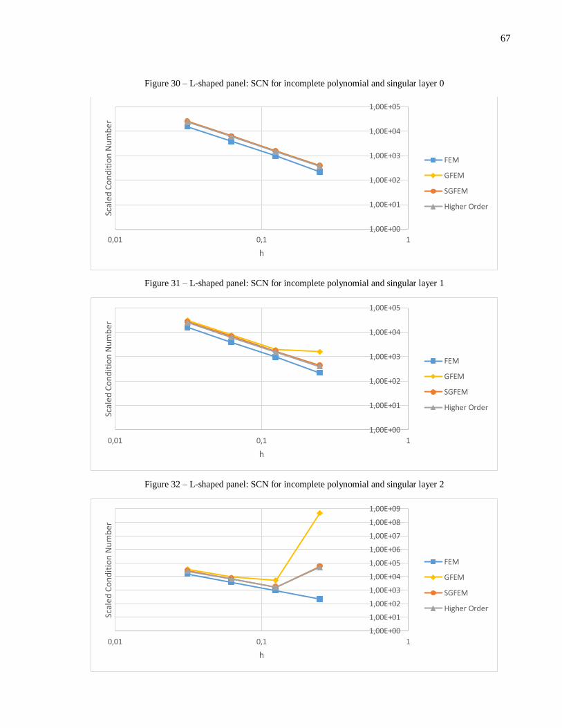
67

Figure 30 – L-shaped panel: SCN for incomplete polynomial and singular layer 0



1,00E+00

1,00E+01

1,00E+02

1,00E+03

1,00E+04

1,00E+05

0,01 0,1 1

Scal

ed C

on

dit

ion

Nu

mb

er

h

FEM

GFEM

SGFEM

Higher Order

1,00E+00

1,00E+01

1,00E+02

1,00E+03

1,00E+04

1,00E+05

0,01 0,1 1

Scal

ed C

on

dit

ion

Nu

mb

er

h

FEM

GFEM

SGFEM

Higher Order

1,00E+00

1,00E+01

1,00E+02

1,00E+03

1,00E+04

1,00E+05

1,00E+06

1,00E+07

1,00E+08

1,00E+09

0,01 0,1 1

Scal

ed C

on

dit

ion

Nu

mb

er

h

FEM

GFEM

SGFEM

Higher Order

68

Finally, when considering the complete polynomial enrichment, as expected, the SCN for the

GFEM and SGFEM are strongly affected, therefore resulting in a bad conditioned stiffness matrix.

Nevertheless, the higher order SGFEM preserves a SCN close to that one obtained for FEM, as

reported in Table 5.

Table 5 – L-shaped panel: SCN for complete polynomial and singular layer 2


1.0

4 x 2 0.25 2.16E+02 1.8E+16 8.40E+16 1.19E+05

8 x 4 0.125 9.43E+02 1.08E+16 6.52E+15 1.63E+03

16 x 8 0.0625 3.87E+03 4.78E+14 4.29E+15 6.43E+03

32 x 16 0.03125 1.56E+04 5.07E+16 3.27E+15 2.57E+04

Despite the better conditioning for the Higher order, using the flat-top partition of unity results in

a worse approximate solution when compared to the SGFEM, as depicted in Figure 33.

Figure 33 – L-shaped panel: h-convergence for complete polynomial and singular layer 2

However, the higher order SGFEM benefits from the mesh refinement, as can be seen in Figure

34. Furthermore, the stress concentration due to the singular enrichment is shown in Figure 35.

0,0001

0,001

0,01

0,1

1

0,001 0,01 0,1 1

Rel

ativ

e er

ror

h

FEM

GFEM

SGFEM

Higher Order

69

Figure 34 – L-shaped panel: effect of mesh refinement

70

Figure 35 – L-shaped panel: nodal stress Sxy for mesh 64 x 32 using different enrichment

7.2 Panel presenting an edge crack

The selected problem, as well an example of a regular mesh adopted for analysis is depicted in

Figure 36.

Figure 36 – Edge cracked panel

71

Sliding supports are prescribed at the left Dirichlet vertical boundary and at the crack tip. The

Dirichlet boundary conditions are imposed using a penalization technique. Uniform distributed

loads are applied at the top and bottom edges. Besides, a gap of 10-4 order is considered to represent

the crack.

Six structured meshes varying from coarse to fine and composed by bilinear quadrilateral elements

are used to analyze the h-convergence, however, for the study of the SCN only the four coarser

meshes are considered due to the loss of accuracy for the finer ones. These meshes present the

following grid arrangements: 4x4, 8x8, 16x16, 32x32, 64x64 and 128x128, according to the

number of elements in the horizontal and vertical directions, respectively.

Analogous to the L-shaped panel, in this example the analysis is made considering four conditions,

aiming to focus on the relative differences, advantages and shortcomings, among the GFEM

versions.

7.2.1 Parameter analysis

The analysis is presented next in terms of the convergence rates of relative errors in displacements

for equals to 0.01, 0.1, 0.2, 0.3 and 0.4. The enrichment considered is the shifted complete second

degree polynomial.

The reference solution refu used in Relation (21) was computed through FEM using a very refined

structured mesh of (2048x2048) elements. The resulting h-convergence curves are presented in

Figure 37.

72

Figure 37 – Edge cracked panel: h-convergence for different values of

As well as in the L-shape example, the smaller the is, the better the approximate solution.

However, if becomes too small, the partition of unity tends to be pretty much similar to the hat

PoU. Then, the scaled condition number increases relatively, already for the coarse mesh, as seen

in Figure 38.

Figure 38 – Edge cracked panel: SCN for analysis

Despite the similarity of the obtained results when comparing the different values of in the range

from 0.1 to 0.4, a small relative difference can be observed. Therefore, 1.0 is chosen for the

next analysis, since comparatively this value has provided the smallest error and the lowest SCN.

0,001

0,01

0,1

1

0,001 0,01 0,1 1

Rel

ativ

e er

ror

h

HIGHER 0.01

HIGHER 0.10

HIGHER 0.20

HIGHER 0.30

HIGHER 0.40

1,00E+00

1,00E+01

1,00E+02

1,00E+03

1,00E+04

1,00E+05

1,00E+06

0,01 0,1 1

Scal

ed C

on

dit

ion

Nu

mb

er

h

HIGHER 0.01

HIGHER 0.10

HIGHER 0.20

HIGHER 0.30

HIGHER 0.40

73

7.2.2 Polynomial enrichment

Shifted complete and incomplete second degree polynomials are considered in this example for the

enrichments applied to the whole set of nodes.

A comparison between GFEM, SGFEM and higher order SGFEM is presented. The main aspects

appraised are the rate of convergence based on the estimated errors in displacements and the scaled

condition number.

The relative errors in displacements were computed using the 2 norm. For the case of incomplete

enrichment, the resulting values are reported in Table 6.

Table 6 – Edge cracked panel: Relative errors for incomplete polynomial enrichment


1.0

4x4 0.25 0.26134 0.17022 0.15184 0.166581834

8x8 0.125 0.14344 0.08548 0.08275 0.089600582

16x16 0.0625 0.07421 0.04378 0.04392 0.047327711

32x32 0.03125 0.03741 0.02209 0.02247 0.024203718

64x64 0.01563 0.01853 0.01088 0.01113 0.012011457

128x128 0.00781 0.00898 0.00515 0.0053 0.005740655

The log x log graphs depicted in Figure 39 show the h-convergence of the relative errors. Even if

this is not a regular problem, as the crack tip induces heavy stress singularity, it can be observed

that the convergence rates are pretty much of the same order comparing the GFEM versions with

FEM.

74

Figure 39 – Edge cracked panel: relative error values for incomplete polynomial and mesh refinement

In Figure 40, the scaled condition number is compared still considering the incomplete enrichment

case. It can be seen that the values obtained with GFEM versions are of the same order as the values

provided by FEM analysis. Once the shape functions resulting from the incomplete enrichment

space verify the linear independence condition, in fact the flat-top option does not have any

advantage over the SGFEM.

Figure 40 – Edge cracked panel: scaled condition number for incomplete polynomial and mesh refinement

However, when considering complete second degree polynomial enrichment, the SCN for SGFEM

is strongly affected, becoming comparable to the bad condition level shown by GFEM, as reported

in Table 7. This is a consequence of the linear dependence among the shape functions introduced

by the crossed term of the enrichment functions vector. However, linear independence is preserved

0,001

0,01

0,1

1

0,001 0,01 0,1 1

Rel

ativ

e er

ror

h

FEM

GFEM

SGFEM

Higher Order

1,00E+00

1,00E+01

1,00E+02

1,00E+03

1,00E+04

1,00E+05

0,01 0,1 1

Scal

ed C

on

dit

ion

Nu

mb

er

h

FEM

GFEM

SGFEM

Higher Order

75

when using flat-Top PoU for constructing the enrichment space. This advantage is clear when

observing the low SCN values, which are comparable in order to the values obtained by the FEM.

Table 7 – Edge cracked panel: scaled condition number for complete polynomial


1.0

4 x 4 0,25 1.16E+02 1.02282E+16 3.07E+17 2.44E+02

8 x 8 0,125 4.89E+02 2.89938E+15 1.75E+16 8.58E+02

16 x 16 0,0625 2.05E+03 1.13806E+16 2.62E+14 3.43E+03

32 x 32 0,03125 8.42E+03 1.05935E+17 2.76E+14 1.38E+04

Once more, using the flat-top PoU results in a limited capacity of approximation and the relative

error is higher than that obtained for the SGFEM, as depicted in Figure 41.

Figure 41– Edge cracked panel: relative error values for complete polynomial and mesh refinement

7.2.3 Singular enrichment

Analogous to the L-shaped panel example, the enrichment using the singular function is now

applied locally around the crack tip according to a three-layer scheme, as shown in Figure 42.

Figure 42 – Edge cracked panel: (a) Layer 0, (b) Layer 1 and (c) Layer 2. The red dots are the enriched nodes

0,001

0,01

0,1

1

0,001 0,01 0,1 1

Rel

ativ

e er

ror

h

FEM

GFEM

SGFEM

Higher Order

76

First of all, for each layer case a comparison between different values of singularn is made using only

the GFEM. Then, after identifying the more convenient value of singularn , a comparison between

the GFEM and SGFEM is presented. In both cases, the comparison is conducted by using the rate

of convergence of the relative error.

The singular function parameters for Relation (17) adopted in this example are such that 1Γ and 2Γ

are both Neumann boundaries and 2 . The resultant enrichment function is:

2 cos 2

k

kkL r

(23)

The h-convergence curves for different layers are presented in the log x log graphs of Figures 43

to 45. For each layer the value ofsingularn varies from 1 to 3.

Figure 43 – Edge cracked panel: h-convergence for singular layer 0 with nsingular varying from 1 to 3


0,001

0,01

0,1

1

0,001 0,01 0,1 1

Rel

ativ

e er

ror

h

GFEM L0 n1

GFEM L0 n2

GFEM L0 n3

77


The rate of convergence slightly improves when increasing the value ofsingularn adopted. Therefore,

looking for a good compromise between precision and reduced computational costs, it is valid to

adopt singularn equals to one for the next analysis.

Once again, the misalignment of the points related to the coarse mesh (4x4) observed in Figure 45

in particular is supposed to be consequent from the significant number of enriched nodes included

in the layer regarding the total number of nodes in the mesh. Differently from the other meshes, in

this mesh all nodes are enriched when applying layer 2, for instance and no blending elements are

presented. However, when passing to the next mesh, the relative error increases as blending

elements arise. Moreover, it is important to note that the singular function is good to approximate

0,001

0,01

0,1

1

0,001 0,01 0,1 1R

elat

ive

erro

r

h

GFEM L1 n1

GFEM L1 n2

GFEM L1 n3

0,001

0,01

0,1

1

0,001 0,01 0,1 1

Rel

ativ

e er

ror

h

GFEM L2 n1

GFEM L2 n2

GFEM L2 n3

78

only the neighborhood of the crack tip. Therefore, no significant gain of approximation can be

noted in the region far away from crack tip.

In Figures 46 to 48, the h-convergence curves for GFEM and SGFEM are presented using different

layers and setting nsingular = 1. It is clear that the SGFEM is able to overcome the shortcoming

caused by the blending elements.

Figure 46 – Edge cracked panel: comparison between methods with respect to h-convergence for singular layer 0


0,001

0,01

0,1

1

0,001 0,01 0,1 1

Rel

ativ

e er

ror

h

FEM

GFEM L0 n1

SGFEM L0 n1

0,001

0,01

0,1

1

0,001 0,01 0,1 1

Rel

ativ

e er

ror

h

FEM

GFEM L1 n1

SGFEM L1 n1

79


7.2.4 Polynomial and singular enrichment combined

Here both polynomial and singular enrichments are combined. The shifted polynomial is applied

to the whole set of nodes, while the singular function is set locally in layers, as in the previous

condition.

The analysis is performed with respect to the rate of convergence based on the relative error and

the SCN. Figures 49 to 51 show the h-convergence curves resulting from the combination of the

singular enrichment in different layers and incomplete polynomial.

Figure 49 – Edge cracked panel: h-convergence curves for incomplete polynomial and singular layer 0

0,001

0,01

0,1

1

0,001 0,01 0,1 1R

elat

ive

erro

r

h

FEM

GFEM L2 n1

SGFEM L2 n1

0,001

0,01

0,1

1

0,001 0,01 0,1 1

Rel

ativ

e er

ror

h

FEM

GFEM

SGFEM

Higher Order

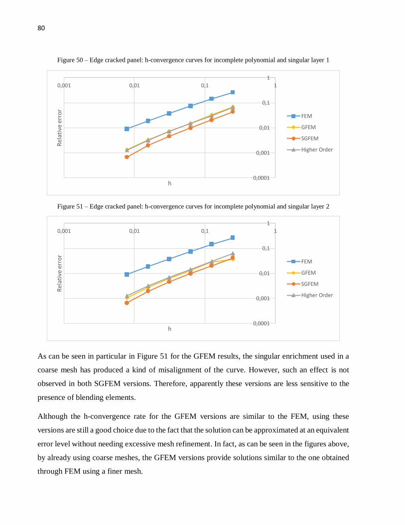
80



As can be seen in particular in Figure 51 for the GFEM results, the singular enrichment used in a

coarse mesh has produced a kind of misalignment of the curve. However, such an effect is not

observed in both SGFEM versions. Therefore, apparently these versions are less sensitive to the

presence of blending elements.

Although the h-convergence rate for the GFEM versions are similar to the FEM, using these

versions are still a good choice due to the fact that the solution can be approximated at an equivalent

error level without needing excessive mesh refinement. In fact, as can be seen in the figures above,

by already using coarse meshes, the GFEM versions provide solutions similar to the one obtained

through FEM using a finer mesh.

0,0001

0,001

0,01

0,1

1

0,001 0,01 0,1 1

Rel

ativ

e er

ror

h

FEM

GFEM

SGFEM

Higher Order

0,0001

0,001

0,01

0,1

1

0,001 0,01 0,1 1

Rel

ativ

e er

ror

h

FEM

GFEM

SGFEM

Higher Order

81

Regarding the SCN, while considering singular enrichment restricted to the layer 0 scheme, the

results for the GFEM versions are close to numbers provided by the FEM, as shown in Figure 52.

However, when the singular function enrichment includes nodes around the corner, the SCN is

badly affected, especially for coarse meshes, as can be observed in Figures 53 and 54. Probably,

the enrichment combination generates shape functions that are almost linearly dependent on those

cases. Even so, the higher order SGFEM seems to be a safer option and the relative small

disturbances in SCN values should not be taken into account as the main purpose of using the

singular function is to capture the stress concentration that occurs in a small neighborhood of the

crack tip.

Figure 52 – Edge cracked panel: SCN for incomplete polynomial and singular layer 0


1,00E+00

1,00E+01

1,00E+02

1,00E+03

1,00E+04

1,00E+05

0,01 0,1 1

Scal

ed

Co

nd

itio

n N

um

be

r

h

FEM

GFEM

SGFEM

Higher Order

1,00E+00

1,00E+01

1,00E+02

1,00E+03

1,00E+04

1,00E+05

0,01 0,1 1

Scal

ed

Co

nd

itio

n N

um

be

r

h

FEM

GFEM

SGFEM

Higher Order

82


Once again, when considering the complete polynomial, the SCN values for the GFEM and

SGFEM are significantly affected. However, the higher order SGFEM keeps a low SCN, with a

still acceptable exception for the coarser mesh, as shown in Table 8.

Table 8 – Edge crack panel: SCN for complete polynomial and singular layer 2


1.0

4 x 4 0.25 1.16E+02 6.3922E+15 6.07E+15 4.27E+05

8 x 8 0.125 4.89E+02 1.51867E+17 1.26E+18 9.25E+02

16 x 16 0.0625 2.05E+03 1.6821E+16 1.12E+15 3.60E+03

32 x 32 0.03125 8.42E+03 2.4264E+15 5.30E+14 1.44E+04

In fact, despite the relative higher SCN for the coarser mesh when using the higher order SGFEM,

this result is still acceptable as it does not point to an ill-conditioned stiffness matrix. Nevertheless,

in spite of using the flat-top PoU lead to a well-conditioned system, the relative error obtained is

comparatively higher than the error of the SGFEM, as shown in Figure 55.

1,00E+00

1,00E+01

1,00E+02

1,00E+03

1,00E+04

1,00E+05

1,00E+06

1,00E+07

1,00E+08

1,00E+09

0,01 0,1 1

Scal

ed

Co

nd

itio

n N

um

be

r

h

FEM

GFEM

SGFEM

Higher Order

83

Figure 55 – Edge cracked panel: h-convergence for complete polynomial and singular layer 2

Nevertheless, the SGFEM using flat-Top PoU benefits from the mesh refinement, as shown in

Figure 56. Furthermore, the stress concentration due to the singular enrichment is presented in

Figure 57.

0,0001

0,001

0,01

0,1

1

0,001 0,01 0,1 1R

elat

ive

erro

r

h

FEM

GFEM

SGFEM

Higher Order

84

Figure 56 – Edge cracked panel: effect of mesh refinement

85

Figure 57 – Edge cracked panel: nodal stress Syy for mesh 64 x 64 for different enrichments

7.3 Panel with multiple corners, polygonal voids and edge cracks

This example aims to show that even if a more complex structure is simulated, the methods hereby

considered are still accurate. This example is similar to the test problem originally proposed in

Strouboulis, Copps and Babuška (2001). The irregular polygonal geometry is shown in Figure 58a.

Figure 58 – Irregular polygonal panel

86

The crack lengths highlighted in red in the figure above are: 127.0a1 and 107.0a2 .

The strong form of the mathematical problem for the linear elasticity, without considering body

forces and the respective boundary conditions are defined as follows:

1

2

3 4 10

( ) 0 on

2 on

0 on

0 on , , ...,

div T

Tn q x y

u

q

where T is the stress tensor.

Taking as a reference the preliminary subdivision of the panel domain in subareas, four structured

meshes varying from coarse to fine were conceived to analyze the h-convergence rate, each one

consisting of bilinear quadrilateral elements. Although, when considering the SCN only the three

coarser meshes were considered due to the loss of accuracy for the finer one.

For a better understanding, Figure 59 depicts the areas defined from the preliminary subdivision of

the panel domain. The meshes were then successively constructed by dividing the edges of the

subareas into 2, 4, 8, 16 parts. In Figure 58b, the mesh where the subareas are divided into 4 parts

is depicted.

Figure 59 – Irregular polygonal panel: subdivision in areas and singular point

87

Shifted incomplete and complete second degree polynomials combined with singular functions

were considered for enrichment. The polynomial was imposed to the whole set of nodes. The

singular enrichment was applied at the corners and crack tips highlighted in Figure 59, following

the layer-schemes 0 and 1, as described in the previous examples.

The corners where the singular function was applied were selected by analyzing the stress

distribution shown by the reference numerical solution. In this solution, the 17 corners highlighted

in Figure 59 presented a more significant stress concentration.

Table 9 lists the parameters adopted and the singular functions used in each of the selected corners.

Table 9 – parameter and singular function for each corner

Corner

number Singular

function

Corner

number Singular

function

1 0.5 cosr 10 0.743723 cosr

2 0.877278 sinr 11 0.769407 cosr

3 0.883286 sinr 12 0.663369 cosr

4 0.811627 sinr 13 0.761295 cosr

5 0.84071 sinr 14 0.750657 cosr

6 0.666667 cosr 15 0.667065 cosr

7 0.662808 cosr 16 0.829467 cosr

8 0.672313 cosr 17 0.5 cosr

9 0.664954 cosr

A comparison between the GFEM versions is presented next. The main aspects evaluated are the

rate of convergence based on the relative errors in displacements and the SCN.

The reference solution refu needed for computing the relative error through expression (21) was

obtained by a FEM analysis using a very refined structured mesh. In this mesh, the edges of the

subareas were divided into 256 segments.

Relative errors in displacements computed using the 2 norm for combined enrichment cases are

presented in log x log scale graphs, as shown in Figures 60 and 61.

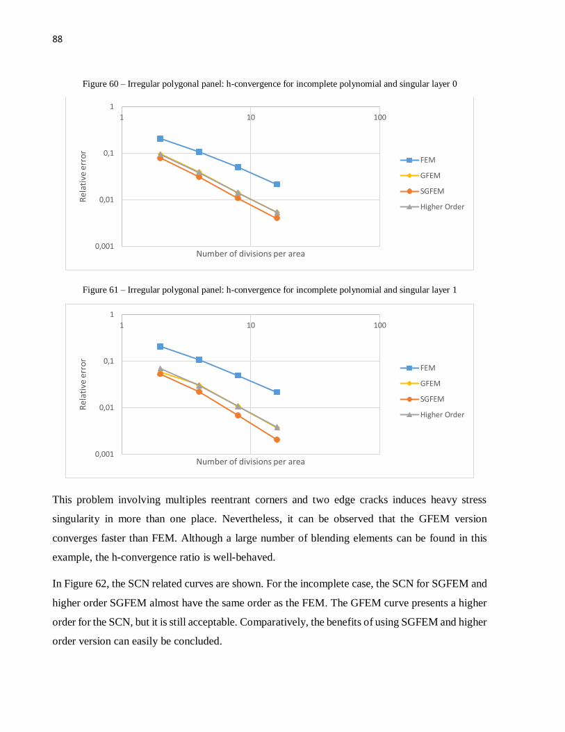
88

Figure 60 – Irregular polygonal panel: h-convergence for incomplete polynomial and singular layer 0

Figure 61 – Irregular polygonal panel: h-convergence for incomplete polynomial and singular layer 1

This problem involving multiples reentrant corners and two edge cracks induces heavy stress

singularity in more than one place. Nevertheless, it can be observed that the GFEM version

converges faster than FEM. Although a large number of blending elements can be found in this

example, the h-convergence ratio is well-behaved.

In Figure 62, the SCN related curves are shown. For the incomplete case, the SCN for SGFEM and

higher order SGFEM almost have the same order as the FEM. The GFEM curve presents a higher

order for the SCN, but it is still acceptable. Comparatively, the benefits of using SGFEM and higher

order version can easily be concluded.

0,001

0,01

0,1

1

1 10 100

Rel

ativ

e er

ror

Number of divisions per area

FEM

GFEM

SGFEM

Higher Order

0,001

0,01

0,1

1

1 10 100

Rel

ativ

e er

ror


FEM

GFEM

SGFEM

Higher Order

89

Figure 62 – Irregular polygonal panel: SCN for incomplete polynomial and singular layer 0

When considering complete polynomial enrichment combined with singular enrichment for layer-

scheme 1, the approximate solution improves compared to FEM, in the way the relative error for a

same mesh is smaller, as shown in Figure 63.

In terms of h-convergence, the SGFEM shows to be the best among the GFEM versions discussed.

However, the complete polynomial contains a parcel which makes the resulting shape functions

linearly dependent. Consequently, the SCN becomes high enough to make the solution less reliable,

Table 10.

Figure 63 – Irregular polygonal panel: h-convergence for complete polynomial and singular layer 1

Despite the higher level of the relative error of the GFEM with respect to the SGFEM, its low SCN

makes the higher order SGFEM a more reliable method.

1,00E+03

1,00E+04

1,00E+05

1,00E+06

1,00E+07

1 10

Rel

ativ

e er

ror


FEM

GFEM

SGFEM

Higher Order

0,001

0,01

0,1

1

1 10 100

Rel

ativ

e er

ror


FEM

GFEM L1

SGFEM L1

Higher Order L1

90

Table 10 – Irregular polygonal: SCN for complete polynomial and singular layer 1

Number of

divisions per area FEM GFEM SGFEM

Higher Order

1.0

2 4.81E+03 1.71146E+16 1.19674E+16 1.86E+04

4 2.46E+04 5.9114E+15 1.13896E+16 9.29E+04

8 1.11E+05 1.2702E+16 5.55485E+16 4.17E+05

Once again, the higher order benefits from the mesh refinement as shown in Figure 64.

91

Figure 64 – Irregular polygonal panel: Effect of mesh refinement.

93

8 CONCLUSION

In this research, new versions of the generalized finite element method were numerically tested

through a combination of polynomial and singular enrichment functions for increasing the

approximation space. The new versions hereby considered were originally conceived to overcome

two major drawbacks that may significantly influence the convergence and stability of the GFEM.

They are the problem of ill-conditioning caused by linear dependencies induced into the solving

system through the adopted enrichment and the appearance of the blending elements when the

enrichment is restricted to a part of the domain.

Three examples allowing the possibility of local enrichment and consisting of structural panels

were considered for performing linear 2-D analysis. The basic geometric features of the examples

herein described were the existence of reentrant corners and cracks, both inducing stress

concentrations restricted to the regions around it. Therefore, in order to capture such localized

effects, the singular function enrichment was explored only in a neighboring region from those

points. Polynomial enrichments were used to capture the smooth parts of the solutions.

In the stable GFEM version, a modification of the enrichment function is proposed aiming to

guarantee stability comparable to the FEM solving linear system. Nevertheless, as concluded from

the examples, linear dependencies still remain when the enrichment is a complete polynomial,

therefore making the solution unreliable. Hence, as already observed in the original formulation, it

was confirmed that the above mentioned modification is not a sufficient condition for stability.

Aiming to further investigate the SCN issue, now considering that high values for it cannot be

completely avoided in the SGFEM, an improved version of the SGFEM was tested numerically.

Once again, the numerical analysis was over the 2-D panels. In conclusion, the higher order

SGFEM fulfilled what was proposed in its formulation, i.e. the scaled condition number

comparable to the FEM values. Therefore, taking the low levels of scaled condition number as the

criterion for comparison, this method appears to be more reliable than the GFEM and SGFEM.

Despite this good feature, it is important to point out that taking the same mesh into consideration,

the higher order SGFEM provides results including a larger error margin when compared mainly

with the SGFEM results.

94

Finally, throughout the tested examples, it was also observed that the blending elements for the

case of singular enrichment do not cause significant harmful effects to the rate of convergence.

95

REFERENCES

Babuška, I.; Osborn, J. E. Generalized finite element methods: their performance and their

relation to mixed methods. SIAM Journal on Numerical Analysis, 1983, vol. 20, no. 3, p.

510-536.

Babuška, I.; Banerjee, U. Stable generalized finite element method (SGFEM). Computer

Methods in Applied Mechanics and Engineering, 2012, 201-204, p. 91-111.

Babuška, I.; Caloz, G.; Osborn, J. E. Special Finite Element Methods for a Class of Second

Order Elliptic Problems with Rough Coefficients. SIAM Journal on Numerical Analysis,

1994, vol. 31, no. 4, p. 945-981.

Daux, C.; Moës, N.; Dolbow, J.; Sukumar, N.; Belytschko, T. Arbitrary branched and

intersecting cracks with the extended finite element method. International Journal for

Numerical Methods in Engineering 2000, 48, p. 1741–1760.

Dolbow, J.; Moës, N.; Belytschko, T. Discontinuous enrichment in finite elements with a

partition of unity method. Finite Elements in Analysis and Design, 2000, 36, p. 235 –260.

Piedade Neto, D.; Ferreira, M. D. C.; Proença, S. P. B. An Object‐Oriented class design for

the Generalized Finite Element Method programming. Latin American Journal of Solids

and Structures, 2013, vol.10, p.1267‐1291.

Duarte, C. A. The hp Cloud Method. PhD dissertation, The University of Texas at Austin,

Austin, TX, USA, 1996.

Duarte, C.A.; Babuška, I.; Oden, J.T. Generalized finite element method for three-

dimensional structural mechanical problems. Computer & Structures, 2000, 77, p. 215-

232.

Duarte, C. A.; Reno, L. G.; Simone, A. A high-order generalized FEM for through-the

thickness branched cracks. International Journal for Numerical Methods in Engineering,

2007, 72, p. 325–351.

Fries, T-P. A corrected XFEM approximation without problems in blending elements.

International Journal for Numerical Methods in Engineering, 2008, v. 75, p. 503-532.

96

Fries, T-P.; Belytschko, T. The generalized/extended finite element method: An overview

of the method and its applications. International Journal for Numerical Methods in

Engineering, 2010, v. 84, p. 253-304.

Griebel, M.; Schweitzer, M.A. A particle‐partition of unity method, Part II: efficient cover

construction and reliable integration. SIAM J. Sci. Comput, 2002, 23(5), p. 1655‐1682.

Gupta, V.; Duarte, C. A.; Babuška, I.; Banerjee, U. Stable GFEM (SGFEM): Improved

conditioning and accuracy of GFEM/XFEM for three-dimensional fracture mechanics.

Computer Methods in Applied Mechanics and Engineering, 2015, 289, p. 355-386

Gupta, V.; Kim, D.; Duarte, A. Analysis and improvements of global–local enrichments

for the Generalized Finite Element Method. Computer Methods in Applied Mechanics and

Engineering, 2012, 245–246, p. 47–62.

Ji, H.; Dolbow, J. On strategies for enforcing interfacial constraints and evaluating jump

conditions with the extended finite element method. International Journal for Numerical

Methods in Engineering 2004, 61, p. 2508 –2535.

Lins, R. M. A posteriori error estimations for the generalized finite element method and

modified versions. Tese (doutorado), Universidade de São Paulo, 2015.

Melenk, J. M.; Babuška, I. The partition of unity finite element method: Basic theory and

applications. Computer Methods in Applied Mechanics and Engineering, 1996, 139, p. 289-

314.

Moës, N.; Dolbow, J.; Belytschko, T. A finite element method for crack growth without

remeshing. International Journal for Numerical Methods in Engineering, 1999, 46(1), p.

131–150.

Simone, A.; Duarte, C. A.; Van der Giessen, E. A Generalized Finite Element Method for

polycrystals with discontinuous grain boundaries. International Journal for Numerical

Methods in Engineering, 2006, 67, p. 1122–1145.

Stroboulis, T.; Babuška, I.; Copps, K. The design and analysis of the generalized finite

element method. Computer Methods in Applied Mechanics and Engineering, 2000, 181, p.

43-69.

Strouboulis, T.; Copps, K.; Babuška, I. The generalized finite element method. Computer

Methods in Applied Mechanics and Engineering, 2001, 190, p. 289-314.

97

Sukumar, N.; Srolovitz, D. J.; Baker, T. J.; Prévost, J. H. Brittle fracture in polycrystalline

microstructures with the extended finite element method. International Journal for

Numerical Methods in Engineering, 2003, 56, p. 2015 –2037.

Szabo, B.A.; Babuška, I. Finite Element Analysis. Wiley, New York, 1991, p. 169±173.

Torre, D. A. F.; Barcellos, C. S.; Mendonça, P. T. Effects of the smoothness of partitions of

unity on the quality of representation of singular enrichments for GFEM/XFEM stress

approximations around brittle cracks. Computer Methods in Applied Mechanics and

Engineering, 2015, 283, p. 243-279.

Zhang, Q.; Banerjee, U.; Babuška, I. Higher order stable generalized finite element

method. Numerische Mathematik, 2014, 128: 1-29, DOI:10.1007/s00211‐014‐0609‐1.

Documents

UNIVERSIDADE DE SÃO PAULO ESCOLA DE … · FERNANDO MASSAMI SATO Numerical experiments with stable versions of the Generalized Finite Element Method CORRECTED VERSION (Original version