Université de Montréal RMN par Département de chimie

Université de Montréal

Étude de la diffusion dans les solutions et les hydrogels polymèrespar spectroscopie RMN et par imagerie RMN

par

Wilms Emmanuel Baille

Département de chimie

Faculté des arts et des sciences

Thèse présentée à la Faculté des études supérieures

En vue de l’obtention du grade de

Phi1osophi Doctor (Ph.D.)

en chimie

Septembre 2004

© Wilms Emmanuel Baille, 2004

-z

o

Université (IIide Montréal

Direction des bibliothèques

AVIS

L’auteur a autorisé l’Université de Montréal à reproduire et diffuser, en totalitéou en partie, par quelque moyen que ce soit et sur quelque support que cesoit, et exclusivement à des fins non lucratives d’enseignement et derecherche, des copies de ce mémoire ou de cette thèse.

L’auteur et les coauteurs le cas échéant conservent la propriété du droitd’auteur et des droits moraux qui protègent ce document. Ni la thèse ou lemémoire, ni des extraits substantiels de ce document, ne doivent êtreimprimés ou autrement reproduits sans l’autorisation de l’auteur.

Afin de se conformer à la Loi canadienne sur la protection desrenseignements personnels, quelques formulaires secondaires, coordonnéesou signatures intégrées au texte ont pu être enlevés de ce document. Bienque cela ait pu affecter la pagination, il n’y a aucun contenu manquant.

NOTICE

The author of this thesis or dissertation has granted a nonexclusive licenseallowing Université de Montréal to reproduce and publish the document, inpart or in whole, and in any format, solely for noncommercial educational andresearch purposes.

The author and co-authors if applicable retain copyright ownership and moralrights in this document. Neither the whole thesis or dissertation, norsubstantial extracts from it, may be printed or otherwise reproduced withoutthe author’s permission.

In compliance with the Canadian Privacy Act some supporting forms, contactinformation or signatures may have been removed from the document. Whilethis may affect the document page count, it does not represent any loss ofcontent from the document

Université de Montréal

Faculté des études supérieures

Cette thèse par articles intitulée:

Étude de la diffusion dans les solutions et ]es hydrogels polymères

par spectroscopie RMN et par imagerie R1VIN

Présenté par:

Wilms Emmanuel Baille

a été évaluée par un jury composé des personnes suivantes:

Professeure françoise Winnik Président rapporteur

Professeur Miche! Lafeur Membre du jury

Professeur Julian Zhu Directeur de recherche

Professeur Brian Amsden Examinateur externe

Professeur Patrice Hiidgen Représentant du doyen

o Thèse acceptée le: \

c Résumé

Les systèmes de libération contrôlée ont suscité un intérêt grandissant dans

plusieurs domaines de recherche. L’étude de la diffusion est très utile pour

déterminer les facteurs influençant le processus de relargage. Nous avons étudié

l’auto-diffusion dans les solutions aqueuses et les hydrogels polymères par la

spectroscopie RMN à gradient de champ pulsé et la diffusion de l’eau à l’intérieur de

comprimés par l’imagerie RMN.

Nous avons déterminé le coefficient d’auto-diffusion (D) d’une série de

diffusants polymères incluant les dendrimères de poly(propylène imine) contenant

des groupements terminaux de triéthylèneoxy méthyle éther (PPI(TEO) avec x = 8,

32 et 64), les polyglycidoles hyperbranchés (PGHBs) et les poly(éthylène glycol)s

(PEGs). Il a été démontré que la masse molaire du diffusant et la concentration en

polymère provoquent une diminution de D alors que D augmente avec la

température. Pour étudier l’effet de la forme des diffusants, la comparaison entre des

molécules de masses molaires similaires mais de formes différentes conduit à une

diminution significative de D en partant de PPI(TEO) à PGHBs puis à PEGs.

L’énergie d’activation (Ea) du processus de la diffusion obtenue est moins élevée

pour le PPI(TEO) comparativement aux deux autres (Epp;(TEo)X <EpGHB <EPEG). Ces

résultats ont permis d’illustrer le rôle déterminant de la forme du diffusant sur le

processus de diffusion. Pour étudier l’effet des interactions diffusant/polymère sur la

diffusion, une série de petites molécules possédant des groupes fonctionnels

différents a été étudiée. La valeur de D obtenue pour chaque diffusant est différente

malgré que leur masse molaire et leur forme soient similaires. Cette différence de D

est associée à une différence d’interactions diffusant/polymère. Le même effet est

obtenu lorsque des matrices de polymère possédant des groupes fonctionnels

différents sont utilisées.

L’ensemble des résultats a été utilisé pour tester l’applicabilité d’un modèle

développé dans notre groupe de recherche (le modèle de Petit et al.). Le modèle

reproduit très bien certains effets étudiés. Cependant, le modèle ne permet pas de

111

décrire adéquatement les effets de la forme du diffusant et des interactions

diffusant/polymère sur le processus de la diffusion.

Une séquence classique d’écho de spin avec sélection de tranche de

l’imagerie RMN a été utilisée pour obtenir des images pseudo-3D de la diffusion de

l’eau à l’intérieur des comprimés d’amidon à haute teneur en amylose en fonction du

temps et de la température. L’analyse quantitative de cette diffusion de l’eau conduit

à une diffusion du type Cas II à 25 °C et la diffusion devient anormale à 37 °C. Par

ailleurs, les images obtenues illustrent un gonflement des comprimés très rapide

relativement au processus de la diffusion de l’eau (moins de 15 heures pour atteindre

son état d’équilibre). Quantitativement, la vitesse du gonflement déterminée

augmente aussi bien avec la température qu’avec une diminution de la taille des

comprimés. De plus, une anisotropie du processus de gonflement est obtenue en

fonction de l’axe. En effet, le gonflement est beaucoup plus rapide dans l’axe de

compression des comprimés.

Mots Clés: Diffusion, RMN à gradient de champ pulsé, Imagerie RMN, NMRI,

alcool polyvinylique, PVA, dendrimère, polymère hyperbranché, poly(éthylène

glycol), PEG, Contramid, amylose

oiv

c Abstract

Controlled release systems have been the subject of increasing interest in

many research fields. The study of the diffusion process in those systems is very

usefiil. We have studied diffusion into aqueous solutions and hydrogels by pulsed

field gradient NMR spectroscopy and water diffusion into tablets by NMR imaging.

We have determined the self-diffusion coefficient (D) of a series of polymeric

diffusants such as polyQropylene imine) dendrimers with triethyleneoxy methyl

ether terminal groups (PPI(TEO) with x 8, 32 and 64), hyperbranched

polyglycidols (HBPG) and linear poly(ethylene glycol)s (PEG). Results obtained

show that D decreases with the molecular weight of the diffusant and with the PVA

concentration. furthermore, increasing values of D are obtained with increasing the

temperature. However, for the effect of the shape of the diffusant, comparison

between diffusants with similar molecular weight but different in the shape leads to a

decrease of D from PPI(TEO) to HBPGs and then to PEGs. Activation energy ofthe

diffusion process obtained is less important for PPI(TEO) than for the two other

difffusants (EppI(TEO)x < EpGHB <EPEG). From these results, it is clear that the shape of

the diffusant is an important parameter of the diffusion process. The effect of the

diffusant/polymer interactions has been also investigated. In this case, a series of

small molecules with different functional groups have been studied. For the

diffusants with similar molecular weight the value of D obtained for each of them is

different. That difference in the D value is associated to the diffusant/polymer

interactions. A difference in the D value is also obtained when polymer matrices with

different functional groups are used.

All these studies were used to test the applicability of a new physical model

developed by our research group (the model of Petit et al.). This model has been

successfully used to describe some studied effects. However, the model in its present

form does flot provide an adequate description of the effects of both shape of the

diffusants and the diffusant/polymer interactions on the diffusion process.

Classic spin echo sequence which allows a slice selection lias been used to

obtain pseudo-3D NMR images of the diffusion process of water into high amylose

V

starch tablets as a function of time and temperature. Quantitative data from these

images show that the water uptake as a function of time is a diffusion Case II type at

25 °C and the diffusion process cornes anornalous at 37 °C. Furtherrnore, images

obtained illustrate that the swelling process is very fast in cornparison to the water

diffusion into the tablet. Swelling takes less than 15 hours to reach equilibrium.

Values obtained from these images also demonstrate that swelling increases with

temperature. However, swelÏing decreases with tablet size. Lastly, the swelling

process is aiways anisotropic and the swelling percent is more important in the

compression axis (for tablet proportion) than the other axis.

Keywords: Diffusion, PfG-NMR, NMR imaging, NMRI, Poly(vinyl alcohol), PVA,

dendrimer, hyperbranched polymer, poly(ethylene glycol), PEG, Contramid, amylose

ovi

Tables des Matières

Résumé Iii

Abstract y

Table des matières vii

Liste des tableaux xii

Liste des figures xiv

Liste des symboles et abréviations xxii

Remerciements xxix

Dédicace xxx

Chapitre 1. Introduction générale

1.1. Système de relargage contrôlé 2

1.2. Processus de la diffusion 4

1.2.1. Diffusion fickienne 4

1.2.2. Diffusion non-Fickienne 7

1.2.3. Diffusion mutuelle et auto-diffusion $

1.3. Modèle théorique de Petit et al 9

1.4. Autres modèles théoriques 12

1.4.1. Théorie hydrodynamique 13

1.4.2. Théorie du volume libre 14

1.4.3. Théorie d’obstruction 15

1.4.4. Modèles combinés 16

1.5. Techniques RMN utilisées 16

1.6. Travaux antérieurs 19

1.7. Objectifs de ce travail 20

1.8. Présentation des travaux 25

1.9. Références 27

Chapitre 2. Self-diffusion of hydrophilic poly(propyleneimine) dendrimers in

vii

, poly(vinyl alcohol) solutions and gels by pulsed field gradient NMR spectroscopy

2.1. Abstract 34

2.2. Introduction 35

2.3. Experimental section 36

2.3.1. Materials 36

2.3.2. 2- [2-(2-methoxyethoxy)ethoxy]acetyl chloride 36

2.3.3. Modified poly(propyleneimine) dendrimers 37

2.3.4. Sample preparation 37

2.3.5. Molecular weight determination 37

2.3.6. Relaxation time measurements 37

2.3.7. Pulsed field gradient NMR measurements 38

2.4. Resuits and discussion 40

2.4.1. NMR characterization 40

2.4.2. Relaxation times measurements 42

2.4.3. Diffusion measurements 43

2.4.3.1 Effect ofpolymer concentration 45

2.4.3.2 Effect oftemperature 51

2.5. Conclusion 59

2.6. Acknowledgment 59

2.7. References and notes 60

Chapitre 3. Self-Diffusion Measurements of Hyperbranched Polyglycidols in

PVA Gels by Pulsed Field Gradient NMR Spectroscopy

3.1. Abstract 64



3.3.1.Materials 66

3.3.2. Preparation ofhyperbranched polyglycidol (HBPG) 66

3.3.3. Size exclusion chromatography (SEC) 66

3.3.4. NMR spectroscopy 66

3.3.5. MALDI-TOF mass spectrometry 67

viii

3.3.6. Pulsed field gradient NMR measurements .67

3.4. Results and discussion 6$

3.4. L Characterization of hyperbranched polyglycidols 6$

3.4.2. Diffusion measurements 73

3.4.2.1. Effect of polymer concentration 76

3.4.2.2. Effect oftemperature $2

3.5. Conclusion $6

3.6. Acknowledgment $7

3.7. References and notes $7

Chapitre 4. Study of Diffusant/Polymer Matrix interactions by PFG NMR

Spectroscopy

4.1. Abstract 92


4.3. Experimental Section 94

4.3.1. Materials 94

4.3.2. Sample Preparation 94

4.3.3. Pulsed Field Gradient NMR Measurements 94


4.4.1. Diffusion Measurernents 95

4.4.1.1. Effect of polymer concentration 95

4.4.1.2. Effect of diffusant molecular weight 96

4.4.1.3. Diffusant/polymer interaction 100

4.4.1.4. Functional group effect 106

4.5. Conclusion 111



Chapitre 5. NMR imaging of high amylose starch tablets: 1. swelling and water

uptake

5.1. Abstract 117

ix

5.2. Introduction .118

5.3. Experimental section .119

5.3.1. Tabletpreparation 119

5.3.2. Magnetic resonance imaging experiments 119


5.5. Conclusion 128



Chapitre 6. NMR imaging of high amylose starch tablets: 2. effect of tablet size

6.1. Abstract 132



6.3.1. Tabletpreparation 134

6.3.2. NMR imaging experiments 134

6.3.3. Measurement of water uptake 136

6.4. Results and discussion 137

6.5. Conclusion 147

6.6. Acknowledgments 147


Chapitre 7. Conclusion générale

7.1. L’étude de la diffusion par la RMN PFG 150

7.1.1. L’effet de la masse molaire du diffusant 151

7.1.2. L’effet de la concentration en polymère 151

7.1.3. L’effet de la température 152

7.1.4. L’effet de la forme du diffusant 153

7.1.5. L’effet des interactions diffusanlpolymère 153

7.1.6. Le modèle de Petit et al 154

7.2. L’imagerie RMN des comprimés d’amylose 155

7.2.1. L’effet de la température 155

X

7.2.2. L’effet de la taille .156

7.3. Travaux futurs 156

7.4. Références 15$

Annexe A. Les techniques de spectroscopie R1’1N et d’imagerie RMN utilisées

dans ce travail

A.1. Principes généraux de la RIvIN 161

A.2. Le phénomène de la relaxation en RMN 163

A.2.1. La relaxation spin-réseau 163

A.2.2. La relaxation spin-spin 166

A.3. Le phénomène de la diffusion en RMN 169

A.3.1. L’écho de spin à gradient de champ pulsé 170

A.3.2. L’écho stimulé à gradient de champ pulsé 174

A.3.3. Les limites de ces méthodes 176

A.4. L’imagerie RMN 177

A.4.1. L’encodage de la fréquence 17$

A.4.2. L’encodage de la phase 181

A.4.3. La sélection de tranche 184

A.4.4. La pseudo méthode 3D en d’imagerie RMN 186

A.4.5. L’effet du contraste 18$

A.5. Références 189

Annexe B. Les résultats expérimentaux 191

Annexe C. Listes des publications 202

xi

Liste des tableaux

Table 2.1. Some characteristics of the modified poly(propyleneimine)

dendrimers 40

Table 2.2. NMR relaxation times for the different 1H signais of the

dendrimers at 25 °C 42

Table 2.3. Self-diffusion coefficients (Do), hydrodynamic radii (Rh), and

fitting kfl2 and y parameters obtained for the dendrimers in aqueous PVA

systems 48

Table 3.1. Determination of the molecular weights of HBPGs by $E and

MALDI-TOF mass spectrometry 70

Table 3.2. Relative abundance of substructure units and degree of branching

(DB) of HBPGs obtained by inverse gated ‘3c NMR spectroscopy 72

Table 3.3. Experimental self-diffusion coefficients (D0), hydrodynamic Radii

(Rh) and fitting parameters k/ and D0 obtained for the HBPG in aqueous

PVA systems 80

Table 4.1. Self-diffusion coefficients (D0), hydrodynamic radii (Rh) and fitting

parameters kfl2 and y obtained in aqueous PVA systems 99

Table 4.2. Fitting parameters values of a and u obtained in aqueous PVA

systems by the use ofeq 4.5 102

Table 5.1. Initial tablet diameter (d0), maximum swelling diameter (dm) and

rate constants of the swelling (Ic) of contramid tablets at two different

temperatures 126

Table 6.1. Physical characteristics ofthe tablets 136

Table 6.2. Parameters obtained by fitting the tabiet sweliing data in figure 6.4

toeq6.2 142

xii

Table 6.3. Parameters obtained by fitting the data in figure 6.5 to eq 6.3 for

the dry diameter and to a linear function for the dry thickness 144

Table 6.4. Parameters obtained by fitting the water uptake data in figure 6.6 to

eq6.4 146

oxlii

G Liste des figures

Figure 1.1. Mécanisme de libération contrôlée d’une molécule active en

fonction du système de libération utilisée, ta) Gonflement de la matrice

polymère suivi de la diffusion du principe actif. (b) Diffusion du principe actif

à travers la couche de polymère 3

Figure 1.2. Variation avec le temps (t) du gradient de concentration d’un

système binaire (produit A et B) 5

Figure 1.3. Schéma illustrant la diffusion d’un diffusant A à travers un fin film

de polymère 6

Figure 1.4. Séquences d’impulsions de la technique RMN à gradient de champ

pulsé. (a) Séquence d’écho de spin et (b) séquence d’écho stimulé 1$

Figure 1.5. Structure de deux dendrimères de poly(propylène imine) contenant

des groupements terminaux de triéthyÏèneoxy méthyle éther (PPI(TEO) où x =

8,32) 21

Figure 1.6. Structure des polymères hyperbranchés de polyglycidols (HBPGs) 21

Figure 1.7. Structures chimiques de la préparation de l’alcool polyvinylique 22

Figure 1.8. Structures chimiques des autres matrices polymères utilisés pour

l’étude du processus de diffusion dans les solutions et les hydrogels de

polymères 23

Figure 1.9. Structures chimiques de l’amylose ta) et de l’amylopectine (b) 24

Figure 2.1. 1H NMR spectra of three different poly(propyleneimine)

dendrimers with hydrophilic triethylenoxy methyl ether terminal groups at 1

wt% in D20 at 25 °C. (A) PPI(TEO)s, (B) PPI(TEO)32, (C) PPI(TEO)64 41

Figure 2.2. Semilogarithmic plot of the attenuation of the dendrimer NMR

signals in a Ï wt % aqueous solution (without PVA) at 25 °C as a function of

xiv

(Gy5)2 (A—6/3). 6 = 1.0 ms, A = 400 ms. Squares, PPI(TEO)8; circles,

PPI(TEO)32; and triangles, PPI(TEO)64 44

Figure 2.3. Dendrimers self-diffusion coefficients as a function of PVA

concentration at 25 °C. Dashed unes are fit to eq 2.7. Squares, PPI(TEO)8;

circles, PPI(TEO)32; and triangles, PPI(TEO)64 46

Figure 2.4. Variation of the kfl2 parameter as a function of the hydrodynamic

radius ofthe dendrimers at 25 °c. The dashed une is drawn only as visual guide 48

Figure 2.5. Dependence of D0 and Rh of dendrimers (A) and PEG (B) on their

molecular weights at 25 °c 50

Figure 2.6. (A) Self-diffusion coefficients and (B) normalized self-diffusion

coefficients (D/D0) of the PPI(TEO)s dendrimer as a function of PVA

concentration at five different temperatures. Dashed lines are fit to eq 2.7 52

Figure 2.7. Dependence of D0 of dendrimers on molecular weight at three

different temperatures. Squares, circles and triangles represent the values

obtained at 5, 25 and 45 °, respectively 53

figure 2.8. Variation of the hydrodynamic radius (Rh) (A) and the i’ parameter

in the mode! of Petit et al. (B) with the temperature for the three dendrimers.

Squares, PPI(TEO)8; circles, PPI(TEO)32; and triangles, PPI(TEO)64 55

figure 2.9. Semilogarithmic plot of the self-diffusion coefficients of the

PPI(TEO)32 dendrimer as a function of reciprocal temperature for four PVA

concentrations. Squares, 0.00 g/mL; circles, 0.06 g/mL; upward triangles, 0.16

g/mL; and downward triangles. 0.26 g/mL 56

Figure 2.10. Variation of the diffusional activation energy with the PVA

concentration for three dendrimers: Squares, PPI(TEO)g; circles, PPI(TEO)32;

and triangles, PPI(TEO)64. The dashed line is drawn only as visua! guide 57

Figure 2.11. Semilogarithmic plot of the kfl2 parameter as a function of

xv

reciprocal temperature for the tbree dendrimers. Squares, PPI(TEO)s; circles,

PPI(TEO)32; and triangles, PPI(TEO)64 58

figure 3.1. Schematic structure of the hyperbranched polyglycidol. Examples

ofthe dendritic segment (D), linear 1,3- segment (L13), linear 1,4-segment (L14)

and terminal segment (T) as indicated by concentric unes 69

Figure 3.2. ‘3C NMR spectrum (A) and DEPT-135 NMR spectrum (B)

obtained for HBPG-l in DMSO-d6. D corresponds to the dendritic segment of

the HBPG and L13 and L14 symbolize respectively the linear 1,3-segment and

the linear 1,4-segment. T represents the terminal segment of HBPGs 71

Figure 3.3. Semiiogarithmic plot of the attenuation of the HBPG NMR signais

in a 1 wt % aqueous solution (without PVA) at 25 oc as a function of

(G76)2 (A—6/3), where 6is fixedto avalue between 0.7 and 1.0 ms and A =

400 ms. Squares, HOD; circles, HBPG-1; up triangles, HBPG-2; down

triangles, HBPG-3 and diamonds, HBPG-4 75

Figure 3.4. Dependence of D0 and Rh of HBPGs on their moiecuiar weights at

25 °c 76

Figure 3.5. (A) HBPG self-diffusion coefficients as a function of PVA

concentration at 25 °C. (B) Normalized self-diffusion coefficients (D/D0) ofthe

HBPG diffusants as a function ofPVA concentration. Dashed unes are fit to eq

3.5. Squares, HBPG-1; circles, HBPG-2; up triangles, HBPG-3 and down

triangles, HBPG-4 78

Figure 3.6. The variation of the self-diffusion coefficients of various diffusants

as a function of PVA concentration. Ail diffusants have similar molecuiar

weight (2000 g/moi) but different shapes. Dashed unes are fit to eq 3.5.

Squares, poly(propyiene-imine) dendrimers; circles. HBPG-4; triangles, linear

PEG $2

Figure 3.7. Self-diffusion coefficients of the HBPG-2 as a flinction of PVA

xvi

concentration at four different temperatures. Dashed unes are fit to eq 3.5 83

figure 3.8. Semilogarithmic plot of the kfl2 parameter as a function of

reciprocal temperature for HBPG diffusants. Squares, HBPG-1; circles, HBPG

2; up triangles, HBPG-3 and down triangles, HBPG-4 84

Figure 3.9. (A) Variation of the apparent activation energy (La) obtained from

the k/32 parameter as a function of the molecular weight (Ma) of the diffusants.

(B) Variation of La as a function of the ratio of Rh/Mfl. (C) Variation of Rh/M

as a function of M of the diffusants. Squares, poly(propylene-imine)

dendrimers; circles, HBPG-4; triangles, linear PEG. The lines are drawn as

visual guides 85

Figure 4.1. Schematic structure of polymer matrices used to study

diffusant/polymer interactions 95

figure 4.2. Variation of the self-diffusion coefficients as a function of PVA

concentration at 25 °C. Dashed unes are fits to eq 4.3. Squares, EG; circles,

DEG; and triangles, TEG 96

figure 4.3. Variation of Rh obtained from eq 4.1 as a function ofthe cubic root

of the molecular weight (M) of the diffusants, including EG, EGMe, EGMe2,

DEG, TEG, TEGMe and TEGMe2. R2 is the root mean square corielation

coefficient 98

Figure 4.4. Dependence of D/D0 as a function of PVA weight fraction (4) at 25

°C. Dashed unes are fits to eq 4.5. Squares, EG; circles, DEG; and triangles,

TEG 100

Figure 4.5. Variation of the self-diffusion coefficients as a function of (A)

PVA and (B) PDEA concentrations at 25 °C. Dashed unes are fits to eq 4.3.

Dependence of D/D0 as a flmction of (C) PVA and (D) PDEA weight fractions

() at 25 0C. Dashed unes are lits to eq 4.5 103

figure 4.6. (A) Change of the self-diffusion coefficients for three diffusants

xvii

with similar molecular weight as a function of PVA concentration at 25 oc.

Dashed unes are fits to eq 4.3. (B) Dependence of D/D0 as a function of PVA

weight fraction () at 25 °c. Dashed unes are fits to eq 4.5. Squares, EG;

circles, EDA; and triangles, 1-lAc 107

figure 4.7. (A)Variation of the self-diffusion coefficients of the EG as a

function of PVA concentrations at five different temperatures. Dashed unes are

fits to eq 4.3. (B) Semilogarithmic plot of the k/32 parameter as a function of

reciprocal temperature for the three diffusants 109

Figure 4.8. (A) The evolution of self-diffusion coefficients of EG into four

polymer matrices and at different polymer concentrations. Dashed unes are fits

toeq4.3 111

Figure 5.1. Schematic diagram of the tablet arrangement for the water uptake

experiment 120

Figure 5.2. Water penetration in high amylose starch tablet at 25°c as a

function of time. Each image is the sum of 4 accumulations with a repetition

time of 2 seconds, yielding an experimental time of 35 minutes. The spatial

resolution in plane is 7$ im, with a suce thickness of 500 iim 121

Figure 5.3. Water penetration in high amylose starch tablet at 37°C as a

function of time. Each image is the sum of 4 accumulations with a repetition

rime of 2 seconds, yielding an experimental time of 35 minutes. The spatial

resolution in plane is 59 Jim, with a suce thickness of 500 tm 122

Figure 5.4. Variation of the diameter of the remaining dry tablet at 25 and

37°C 123

Figure 5.5. Swelling of high amylose starch tablet as a function of time at 25

and37°c 124

Figure 5.6. Advance of solvent front expressed as r, the distance of the solvent

front from the edge of the tablet toward the center of the tablet, at 25 and 37°C

xviii

as a function of immersion time .126

Figure 5.7. Spin density profiles of water (water gradient) extracted from

images obtained at 25 (A-C) and 37°C (D-f) at short immersion times 127

Figure 6.1. Schematic diagram of the tablet arrangement for the NMRI

experiment 135

Figure 6.2. The spin-echo pulse sequence used to acquire two-dimensional

NMR image. TR and TE are the recovery time and the echo time, respectively.

G, G and Gr represent the suce, phase and read gradients, respectively 136

Figure 6.3. NMR images showing the water penetration into Contramid-I tablet

at 37 °C at different times. Each image is the sum of 4 accumulations with a

repetition time of 2 s, yielding an experimental time of 35 min. The nominal

spatial resolution in plane is 7$ 11m, with a suce thickness of 500 im 137

Figure 6.4. Swelling in both axial (O) and radial (.) directions of Contramid-I

(A) and Contramid-II (B) tablets. Solid lines show fit ofthe data to eq 6.2 141

figure 6.5. Variation of the dry diameter (A) and the dry thickness (B) of the

tablet for Contramid-1 (o) and Contramid-II (.) samples. Solid lines show fits

of the data to eq 6.3 and to a linear function for the diameter and the thickness,

respectively 143

Figure 6.6. fractional water uptake of Contramid-I (O) and Contramid-II t.) at

37 °C as a ftmction ofthe square root of immersion time. Solid unes show fit of

the data to eq 6.4 145

Figure A.1. (a) La précession du moment magnétique nucléaire (p) d’un noyau

placé dans un champ magnétique B0 dans la direction de l’axe z. (b)

Orientations possibles du moment angulaire de spin nucléaire pour I = 162

figure A.2. (a) Distribution de la précession nucléaire des moments

magnétiques d’un noyau de spin ‘/2. (b) Le vecteur de magnétisation résultant,

xix

M0 .162

Figure A.3. Séquence d’impulsion de la technique d’inversion récupération 164

Figure A.4. La variation de la magnétisation et l’intensité du signal en fonction

du temps r après l’application du 90° 165

Figure A.5. Variation de l’intensité du signal en fonction du temps r pour la

séquence d’impulsion d’inversion récupération 166

Figure A.6. Séquence d’impulsion d’écho de spins de Carr-Purcell-Meiboom

Giil 16$

Figure A.7. Évolution du système de spins selon la séquence d’impulsion

CPMG 162

Figure A.8. Variation de l’intensité de l’écho en fonction du nombre de boucle

n pour la séquence d’impulsion CPMG 169

Figure A.9. Séquence d’impulsion d’écho de spin de gradient de champ pulsé

et l’intensité de l’écho obtenue après un temps 2r sans la diffusion et avec la

diffusion 171

Figure A.1O. L’atténuation de l’intensité de l’écho dans le cas de l’éthylène

glycol (EG) et de l’eau résiduelle (HOD) en fonction de la force du gradient de

champ magnétique appliquée (ô 1.1 ms et A 60 ms à 25 °C) 173

Figure A.11. Effet du gradient de champ pulsé sur l’atténuation de l’intensité

de l’écho dans le cas de l’éthylène glycol (EG) et l’eau résiduelle (HOD) 174

Figure A.12. Séquence d’impulsion d’écho stimulé de gradient de champ pulsé

et l’écho (ou la magnétisation) obtenu après le temps r = 2ri + z sans de la

diffusion et avec de la diffusion 175

Figure A.13. (a) Variation des temps de relaxation spin-spin (T2) et (b) spin

réseau (T1) avec la rigidité de la molécule et la rigidité de son environnement 177

xx

Figure A.14. L’encodage de la fréquence de précession. (a) La séquence

d’impulsion. (b) L’échantillon dans le plan zx. (c) et (d) Les profiles obtenus

lorsque le gradient de champ est appliqué selon les axes z et x respectivement 180

Figure A.15. L’encodage de phase. (a) La séquence d’impulsion pour un

incrément linéaire de la force du gradient de champ. (b) Exemple de déphasage

résultant de l’application de deux gradients de différente force (G. et G, ) 182

Figure A.16. Séquence d’impulsion ccspin-warp» utilisant l’écho de spin de

Hahn 183

Figure A.17. La sélection de tranche par imagerie RMN. (a) La séquence

d’impulsion. (b) La tranche de l’échantillon sélection par la séquence

d’impulsion illustrée en a 185

Figure A.18. La séquence d’écho de spin du type «spin-warp» avec une

impulsion sélective de 90° 187

Figure Ad9. Pénétration d’un mélange de trois produits dans une tige de

polyamide. (a) Distribution de l’isooctane, du toluène et de l’éthanol. (b)

Distribution de l’isooctane. (c) Distribution du toluène 18$

xxi

Liste des symboles et abréviations

1. Symboles et abréviations utilisés pour les produits chimiques

HAc Acide acétique

ARNm Acide ribonucléique messager

ATP Adénosine triphosphate

ContramidTM Comprimé à base d’amylose et d’amylopectine

DEA Diéthylamine

DEGMe Di(éthylene glycol) méthyl éther

DMSO-d6 Diméthyl sufoxide deutéré

EG Éthylène glycol

HBPGs Hyperbranched polyglycidols

PEGs-x Poly(éthylène glycol) de poids moléculaire x

PEO Poly(éthylène oxide)

PNNDEA Poly(N,N-diéthyl acrylamide)

PPI(TEO) Dendrimère de Poly(propyÏèneimine) contenant x groupes

terminaux de triéthylèneoxy methyl éther

PVA Alcool polyvinylique

TEA Triéthylamine

TEG Tri(éthylène glycol)

TEG-Me Tri(éthylène glycol) méthyl éther

TEG-Me2 Tri(éthylène glycol) diméthyl éther

TEO Triéthylènoxy méthyl ether

xxii

Q2. Symboles et abréviations utilisés pour les différentes équations et Méthodes

a 1) Longueur d’un segment de chaîne

2) Paramètre du modèle de diffusion de Petit et al.

Concentration du produit A (g/mL)

e 1) Concentration de polymère (g/mL)

2) Constante pré-exponentielle

ct Concentration critique, ou concentration de chevauchement des

chaînes de polymère (gImL)

DA Coefficient de diffusion du produit A

Dm Coefficient de diffusion mutuel

D Coefficient d’auto diffusion dans une solution polymère (m2/s)

Do Coefficient d’auto diffusion dans le solvant pur (m2/s)

Coefficient d’auto diffusion lorsque la température tend vers

l’infini (m2/s)

d ou l Diamètre du comprimé gonflé

do Diamètre initial du comprimé

dmax OU 1max Diamètre maximum du comprimé gon±é

DB Degré de branchement d’un polymère hyperbranché

Diamètre de la partie sèche du comprimé

D Segment dendritique d’un polymère hyperbranché

dc/dx Gradient de concentration le long de l’axe x

AE Hauteur de la barrière d’énergie potentielle selon le modèle de Petit

et al.

Ea Énergie d’activation d’un processus dynamique en solution

(kJ/mol)

f Préfacteur de fréquence

JA Flux de matière diffusant par unité de surface et par unité de temps

k Fréquence de saut d’une molécule selon le Modèle de Petit et al.

Constante de Boltzmann (1.380658 x 1023 JK’)

Constante de vitesse de gonflement

lcd Constante de vitesse de pénétration de l’eau dans le comprimé

xxiii

k Constante de vitesse de pénétration de l’eau dans le comprimé

kdiss Constante de vitesse de dissolution du comprimé

L13 Segment linéaire 1,3 du polyglycidols hyperbranchés

Ls14 Segment linéaire 1,4 du polyglycidols hyperbranchés

n 1) Constante tirée de la théorie d’échelle

2) Exposant indiquant une diffusion fickienne, non-fickienne et

anormale

M Masse molaire (g/mol)

Masse molaire en nombre d’un polymère (g/mol), généralement

obtenu par chromatographie d’exclusion stérique (SEC)

Masse molaire en poids d’un polymère (g/mol), généralement

obtenu par chromatographie d’exclusion stérique (SEC)

MH20 Masse d’eau à l’intérieur du comprimé

Masse du comprimé sec

N Nombre d’Avogadro

P Probabilité

R Constante des gaz parfaits (8.31451 Lmol’K’)

Rh Rayon hydrodynamique d’une molécule

Rg Rayon de giration d’une molécule

Rayon d’une molécule diffusante

Rayon d’une chaîne de polymère

T Température (°C ou K)

Tg Température de transition vitreuse

1$ Segments terminaux d’un polymère hyperbranché

t Temps d’immersion dans l’eau des comprimés

VA Volume du produit A (mL)

Volume critique

Vf Volume libre

V Volume spécifique partiel

1) fraction volumique de polymère

2) fraction massique de polymère

xxiv

K Constante tirée du modèle théorique d’Amsden

Potentiel chimique

y Paramètre du modèle de diffusion de Petit et al. caractérisant un

système polymère-solvant

y Paramètre du modèle de Phillies représentant les interactions

diffusant’polymère

/3 Constante tirée de la théorie d’échelle de «de Gennes»

q Viscosité d’une solution de polymère (Pas.s)

rio Viscosité du solvant (Pas.s)

Longueur de corrélation d’une solution polymère semi-diluée

Y Paramètre du modèle théorique de Lustig et Peppas

cL 1) Exposant de Flory

2) Paramètre de l’équation de frisch

fraction de sites occupés par un monomère lorsque la solution de

polymère est prise comme étant un réseau périodique

x Paramètre d’interaction de Flory-Huggins

SEC Chromatographie d’exclusion stérique ($ize exclusion

chromatography)

MALDI-TOF Matrix-assisted laser desorption ionization time-of-flight

oxxv

3. Symboles et abréviations utilisés en résonance magnétique nucléaire

CPMG Séquence d’impulsion classique de Carr-PurceÏl-Meiboom-GiIl

(classical pulse sequences of Carr-Purcell-Meiboom-Gill)

DEPT- 135 Distortionless enhancement by polarization transfer

FLASH Fast low angle shot imaging

FBPR Filtered back projection-reconstruction

RMN Résonance magnétique nucléaire

NMR Nuclear magnetic resonance (voir RMN)

NMRI Imagerie de resonance magnétique nucléaire (nuclear magnetic

resonance imaging)

PFG Pulsed field gradient

TF Transformée de Fourier

SE Spin echo sequence (séquence d’écho de spin)

STE $timulated echo sequence (séquence d’écho stimulé)

STEAM Stimulated echo acquisition mode

Impulsion de 90° selon l’axe i

1$Oj Impulsion de 1800 selon l’axe j

1H Proton

Carbone 13

Fluor 19

Phosphore 31

xxvi

4. Symboles et abréviations utilisés pour les différentes équations analytiques en

résonance magnétïque nucléaire

30 Champ magnétique

Bi Champ magnétique excitateur

D Coefficient d’auto diffusion dans une solution polymère (m2/s)

y Rapport gyromagnétique du proton (rad.s’.T’)

G Intensité du gradient de champ magnétique (T/m)

G Intensité du gradient de champ selon l’axe z

h Constante de Planck (6.6260755xl0341s)

h Constante de Planck divisée par 27t

I Nombre quantique de spin nucléaire

I Intensité du signal RMN en présence de gradient

k Intensité du signal RMN en absence de gradient

k Constante de proportionnalité

k Variable tiré de l’équation analytique de la séquence d’impulsion

inversion récupération

M0 Magnétisation à l’équilibre (magnetization at equilibrium)

M 1) Magnétisation pour un temps de récupération dans le cas de la

séquence d’impulsion inversion récupération

2) Magnétisation pour un nombre paire “n” d’échos dans le cas de

la séquence d’impulsion CPMG

M Magnétisation selon l’axe x

M Magnétisation selon l’axe y

M Magnétisation selon l’axe z

n Nombre d’échos

Population de spin en position Œ (parallèle à la direction de Bo)

Population de spin en position 13 (anti-parallèle à la direction de

Bo)

j Vitesse de la relaxation spin-réseau

R2 Vitesse de la relaxation spin-spin

C

xxvii

$ Intensité du signal dans une expérience d’imagerie RMN

TE Temps d’écho (echo time)

TR Temps de répétition (repetition time)

t1 1) Délais entre les impulsions de 900 et 180° de la séquence

d’écho de spin

2) Délais entre les deux premières impulsions de 90° de la

séquence d’écho stimulé

t2 Temps entre la deuxième et la troisième impulsions de 90° de la

séquence d’écho stimulé

T1 Temps de relaxation spin-réseau

T2 Temps de relaxation spin-spin

6 Temps d’application du gradient magnétique (ms)

A Temps entre deux gradients (ms)

r 1) Temps de récupération pour la séquence d’impulsion inversion

récupération

2) Temps d’écho pour la séquence d’impulsion CPMG

p Densité de spin

p Moment magnétique nucléaire

Vitesse angulaire

fréquence de Larmor

y fréquence de résonance

Largeur de la bande

Modulation de phase

oxxviii

c Remerciements

Les travaux présentés dans cette thèse ont été réalisés au département de

chimie de l’Université de Montréal sous la direction du Professeur Julian X.X. Zhu

que je souhaite remercier grandement pour m’avoir offert l’opportunité de réaliser ce

projet de doctorat dans son groupe de recherche. Je tiens aussi à le remercier pour son

indéfectible appui et son encouragement sans faille pendant les cinq dernières années.

J’aimerais remercier le Docteur Minh Tan Phan Viet. Directeur du

Laboratoire Régional de RMN pour son aide ainsi que Mme Sylvie Bilodeau et M.

Robert Mayer pour leur gentillesse et leur grande disponibilité.

Je tiens également à remercier mes collègues de laboratoire passés et présents

(Aime, Amina, Carl, Chen, Damien, David, Eider, Guillaume, Héloïse, Huiyou,

Junhua, Juntao, Laurent, Marc, Mathilde, Mohand, Mu, Qiang, Sophie, Stephan,

Sumitra, Véronic, Zhengji) avec lesquels il ffit un plaisir de travailler. Mes

remerciements s’adressent aussi à Mme Line Laurin pour sa gentillesse et sa grande

disponibilité.

Je souhaite remercier les étudiants du groupe du Prof. Michel Lafleur

(Sungiong et Jaclin) avec qui j’ai partagé le temps d’utilisation de l’appareil RMN.

Enfin, j’aimerais remercier à titre personnel mon grand ami Cédric Malveau avec qui

j’ai eu un grand plaisir de travailler.

La réalisation de ce projet a été rendue possible grâce a l’appui financier des

fonds de recherche du CRSNG et du fQRNT.

oxxix

Je dédie cette thèse aux membres de mafamille (Kethoue, Layla, William,

Rosita et mes parents) en reconnaissance

pour leur inestimable support et encouragement.

G

xxx

Introduction générale

Les matériaux polymères ont connu un essor fulgurant durant le siècle passé.

Grâce à leur grande polyvalence et leur faible coût de production, ces matériaux sont

de nos jours utilisés dans presque tous les secteurs industriels. Parmi ceux-ci, citons

• Le textile les fibres synthétiques (polyamides, polyesters, polyacryliques

et polyuréthanes) et les fibres naturels (celluloses) [1].

• L’énergie les piles au lithium-polymère (poly(éthylène succinate),

poly(éthylène adipate) et poly(oxide éthylène)), les piles à combustion

(Nafion et poly(éther éther cétone)) [2-4].

• L’agro-alimentaire les emballages (polyéthylène et polystyrène) [5].

• Le cosmétique les produits de soin personnel (chitosan et

hydroxyéthylcellulose) [6, 7].

• Les sciences pharmaceutiques les biocapteurs (polyaniline,

polyacétylène et polythiophène), les bioséparateurs

(poly(isopropylacrylamide), poly(L-lisine), poly(éthylène glycol)) [8-11].

• La médecine : les prothèses (polyuréthane, polysilicone, poly(acide

lactique) et polycarbonate) et la peau artificielle (chitosan) [12-15].

Malgré l’omniprésence des matériaux polymères, il reste encore de beaux défis

scientifiques à relever. On peut citer en exemple, l’utilisation des matériaux

polymères (par exemple des hydrogels) comme matrice ou vecteur lors de la mise en

oeuvre de systèmes de libération contrôlée de principes actifs [19-21]. En effet,

qu’elles soient d’origine naturelle ou synthétique, les macromolécules offrent

d’immenses possibilités dans ce domaine en pleine expansion. Grâce aux systèmes de

relargage contrôlé impliquant les matériaux polymères, nous pouvons moduler la

libération d’un agent actif à vitesse constante sur une période prédéfinie [22]. Il est

également possible d’adapter la libération de manière à la rendre cyclique [22-24].

De même, la libération peut être déclenché par un stimulus externe (par exemple le

pH ou la température). En plus de ces avantages, les systèmes de relargage contrôlé

permettent sur un plan thérapeutique de réduire ou d’éliminer les principaux

1

problèmes que l’on rencontre lors de l’administration traditionnelle de médicaments,

en particulier, la protection du principe actif contre une éventuelle dégradation ou

métabolisation par le milieu biologique [19]. Ils permettent d’éliminer

l’administration périodique [20]. Cependant, leur principal avantage est qu’ils

permettent une meilleure distribution du médicament aux tissus ciblés [21]. Tout ceci

conduit à une plus grande activité thérapeutique bien que la quantité d’agents actifs

utilisés soit nettement moindre que celle nécessaire à l’administration traditionnelle.

1.1. Système de relargage contrôlé

La mise en oeuvre d’un système de relargage contrôlé impliquant le polymère

comme excipient s’effectue selon deux méthodes de préparation bien différentes.

Dans la première, le polymère et le composé actif sont mélangés uniformément à

l’état sec. Dans la seconde, on utilise le polymère sous la forme d’une membrane à

l’intérieur de laquelle on incorpore la molécule active. Malgré cette différence, ces

deux systèmes présentent le même genre de défi. En effet, pour arriver à moduler le

relargage sur une période de temps préétablie pour des applications pharmaceutiques

ou autres, nous devons comprendre comment les propriétés physico-chimiques de la

molécule active influencent ce processus. Il est aussi déterminant de comprendre

comment la matrice polymère affecte le relargage de la dite molécule. En ce sens,

l’influence de facteurs tels que la température, le pH. la concentration en polymère, la

masse molaire du polymère et celle du composé actif doit être élucidée. Nous devons

aussi bien comprendre le rôle d’autres facteurs tels que la forme de la molécule

active, les groupes fonctionnels et les interactions spécifiques (par exemple des

interactions chimiques ou Coulombiennes) sur le processus de libération.

C’est dans cette optique que de nombreuses études portant sur les effets de la

matrice polymère lors de la libération de principes actifs sont apparues durant les

deux dernières décennies [19, 25-33]. Ces études touchent essentiellement les

systèmes de libération contrôlée dans lesquels la matrice polymère subit:

• une hydrolyse ou une érosion.

• un clivage enzymatique ou un changement de pH du milieu (lorsque la

molécule active est reliée à la matrice par des liens covalents).

7

C. un gonflement lorsque la matrice est placée dans une solution donnée (par

exemple le liquide biologique).

• une transition solution-gel.

La figure l.la illustre l’exemple d’un système de libération dont le relargage est

contrôlé simultanément par le processus de gonflement de la matrice polymère et le

processus de diffusion de la molécule active.

a

Gb

Temps

Figure 1.1. Mécanisme de libération contrôlée d’une molécule active en fonction du

système de libération utilisée. (a) Gonflement de la matrice polymère suivi de la

diffusion du principe actif. (b) Diffusion du principe actif à travers la couche de

polymère.

La figure 1 .lb illustre le cas d’un système de réservoir contenant le principe actif (la

partie bleue) entouré d’une couche ou d’une membrane de polymère d’une épaisseur

et d’une densité préalablement définies. L’agent actif à l’intérieur du réservoir peut

C être à l’état solide, en solution diluée ou en solution très concentrée. La libération du

3

principe actif s’effectue via un processus de diffusion fortement contrôlé par

l’épaisseur et la densité de la membrane polymère.

1.2. Processus de la diffusion

La diffusion joue un rôle crucial dans la régularisation de la vie. On n’a qu’à

citer l’exemple du transport intra et extracellulaire du glucose, du Na et du Ca2 à

travers les membranes plasmiques [34]. On peut également citer l’exemple du

transport intra et extracellulaire des protéines, de l’ARNm et de l’ATP dans le cas des

cellules eucaryotes [34]. C’est aussi un phénomène très important dans de

nombreuses applications industrielles. Cependant, le processus de diffusion demeure

aujourd’hui encore dans beaucoup de situations un phénomène très complexe à

expliquer. De manière simpliste, la diffusion est définie comme un processus par

lequel la matière est transportée de manière aléatoire d’un point à un autre [35]. Ce

transport est fortement influencé par les propriétés physico-chimiques de la molécule

qui diffuse (masse molaire, groupes fonctionnels, etc.) de même que par les

propriétés physico-chimiques du milieu dans lequel la molécule diffuse (type de

matrice, concentration, température, viscosité, groupes fonctionnels, etc.). Ce sont ces

influences qui rendent le processus de la diffusion tellement complexe. L’étude du

processus de diffusion a conduit à un double classement du phénomène, la diffusion

dite f ickienne et la diffusion dite non-fickienne.

1.2.1. Diffusion Fickienne

Le processus de diffusion tel que défini par fick (première loi de Fick) peut

être illustré en prenant le cas de l’expérience du réservoir divisé en deux

compartiments séparés par une membrane imperméable (Figure 1.2). Dans chacun

des compartiments, on place un produit pur. Par exemple, dans un compartiment

(défini comme A) on place un volume VA d’un produit A pur et dans l’autre

compartiment (défini comme B) on place un volume VB d’un produit B (en bleu, voir

figure 1.2 au temps t = O). Lorsque la membrane est retirée, on observe une

coloration du compartiment A et une diminution de la coloration du compartiment B

(Figure 1.2 au temps t> O). On dit que le compartiment A s’est enrichi en produit B

alors que le compartiment B s’est enrichi en produit A.

4

Après un temps plus ou moins long (t—> cia), on n’observe plus de transfert net de

produit A ni de produit B. On dit alors que le système est à l’équilibre. Le coefficient

de diffusion (D) pour chacun des deux produits est défini par la première loi de

diffusion de Fick [35, 36]

(1.1)

JB—DB—— (1.2)dx

JA et JB correspondent au flux de matière diffusant en une dimension (selon l’axe x)

et par unité de temps; DA et DB sont les coefficients de diffusions respectifs des

produits A et B; CA et e8 sont les concentrations respectives des diffusants A et B, x la

distance, dc/dx représente le gradient de concentration le long de l’axe x. Le signe

négatif illustre le fait que la diffusion se fait dans la direction opposée au gradient de

concentration. Ce processus, illustré à la Figure 1.2, représente un des cas les plus

A B

/

t=O t>O t—>c/X

Figure 1.2. Variation avec le temps (t) du gradient de concentration d’un système

binaire (produit A et B).

5

simples de l’application de la première loi de Fick (c’est aussi le cas des systèmes

gazeux).

Le processus de diffusion devient plus complexe lorsqu’on s’attaque à la

diffusion dans les matrices polymères. Contrairement au cas précédent, la diffusion

ne dépend pas seulement de la température, de la taille des diffusants et de la

viscosité du milieu (ou la pression lorsqu’on est à l’état gazeux) mais elle dépend

aussi de la concentration en polymère, du degré de gonflement de la matrice

polymère, de même que des interactions entre le diffusant et le polymère. Le cas le

plus simple de la diffusion dans les polymères est illustré à la figure 1.3. Cette figure

montre le cas de la diffusion d’un diffusant A à travers un film de polymère. La

molécule A, placée du coté CA0 (le coté où la concentration en A est la phis élevée),

diffuse à vitesse constante à travers le film de polymère d’une épaisseur 1 pour

aboutir au coté CA1 (le coté où la concentration en A est la plus faible).

Figure 1.3. Schéma illustrant la diffusion d’un diffusant A à travers un fin film de

polymère.

Pour déterminer le flux de matière et la concentration de la molécule A dans ce film

de polymère, nous devons d’abord définir une balance de la masse (Ax) à une

Ax

6

c position donnée à l’intérieur du film [37]. Cette variation linéaire de la concentration

de A à travers le film conduit à une expression du type Fickien.

JA=—DA-=-(cA0—cA,) (1.3)

Les processus de diffusion illustrés par les Figure 1.2 et 1.3 montrent le cas d’une

diffusion du type Ficlden (appelé également Cas I). La diffusion Fickienne est

souvent observée dans les matrices de polymère lorsque la température est au-dessus

de la température de transition vitreuse (‘g) du polymère [3$-41]. Dans ces

conditions, le polymère possède une plus grande mobilité, facilitant ainsi la diffusion

à travers la matrice polymère. On dit alors que la vitesse de la diffusion (R,t) est plus

faible que la vitesse de relaxation du polymère (Rrj) [37-40]. Ainsi, un fort gradient

de concentration du diffusant dans la matrice polymère est observé.

Mathématiquement, on caractérise un tel système par l’expression suivante:

M=Dt (1.4)

Mt étant la quantité d’une espèce donnée absorbée par mètre carré de matrice de

polymère à un temps t et n est égale à 0.5 pour la diffusion Fickienne. Par ailleurs, il

existe de nombreux systèmes que la première loi de Fick ne peut décrire

adéquatement. Le processus de diffusion dans ces systèmes est alors dit non-Fickien.

1.2.2. Diffusion non-Fickienne

La diffusion non-Fickienne est souvent observée dans les systèmes polymères

lorsque les mesures sont effectuées à une température inférieure à la Tg du polymère.

Il est bien connu qu’en dessous de la Tg la mobilité du polymère est restreinte

considérablement, ce qui a pour conséquence de ralentir de beaucoup la diffusion à

l’intérieur de la matrice polymère. L’étude de la diffusion dans ces systèmes conduit

à deux processus de diffusion non-fickienne connus sous le nom de Cas II et

C’ diffusion anormale. Dans le cas du processus de diffusion Cas II, la vitesse de

7

diffusion du solvant est beaucoup plus rapide que la vitesse de relaxation du

polymère [37-40]. La principale caractéristique de la diffusion Cas II est une

augmentation rapide de la concentration du solvant dans les parties gonflées de la

matrice alors que seulement une fine couche du solvant pénètre dans la partie sèche

de la matrice [3 7-401. On observe aussi peu de variation de la concentration du

solvant dans la région gonflée de la matrice. La fine couche servant à la pénétration

avance à une vitesse constante, ce qui aboutit à une proportionnalité entre la distance

parcourue par le front de diffusion et le temps [37-40]. Ce type de processus de

diffusion est généralement représenté par l’équation 1.4 mais n est égale à 1.

La diffusion anormale est définie comme un processus dans lequel la vitesse

de diffusion du solvant est similaire à la vitesse de relaxation du polymère. C’est

aussi un processus intermédiaire à la diffusion fickienne et ta diffusion Cas II. Ainsi,

la quantité d’une espèce absorbée par mètre carré de matrice de polymère à un temps

t est proportionnelle à l’exposant n, n étant compris entre 0.5 et l[37-40].

1.2.3. Diffusion mutuelle et auto-diffusion

La figure 1.2 illustre assez bien le cas d’un processus de diffusion dit

diffusion mutuelle. En effet, la diffusion mutuelle est caractérisée par un transport net

de la matière (c’est-à-dire J 0) de chaque espèce en direction opposée à la région de

sa plus forte concentration. Cela ne signifie cependant pas que la diffusion mutuelle

soit nécessairement ficldenne. Un seul coefficient de diffusion (Dm) est obtenu pour

les deux produits (produit A et produit B) bien que le coefficient de diffusion

intrinsèque de chaque espèce puisse être très différent [39-42].

Dm = VAcA(D— ‘A) + DA (1.5)

L’équation 1.5 illustre la dépendance de Dm (le coefficient de diffusion mutuelle) à la

concentration (CA) et au volume (VA) du produit A. DA et D sont les coefficients de

diffusion respectifs des produits A et B purs.

En ce qui concerne le processus d’auto-diffusion, il peut être défini par l’état

C’ d’équilibre de transfert de la matière, c’est-à-dire lorsque t —cc (voir figure 1.2). On

8

dit alors que la molécule à un mouvement Brownien. En se basant sur la première loi

de fick, on peut aussi définir l’auto-diffusion comme étant un processus sans

gradient de concentration (dc/dx = O), donc un flux global nul (J 0) [42]. Ainsi, un

coefficient de diffusion est obtenu pour chaque diffusant. Ce coefficient de diffusion

est défini par l’expression suivante [35]

DA=DcAIA =RTD (1.6)

0lncA 3IflCA

D étant le coefficient d’auto-diffusion de l’espèce A, p est le potentiel chimique et

aA l’activité thermodynamique de l’espèce A. Une expression similaire peut aussi

être utilisée pour caractériser l’espèce B. Sur un plan pratique, le processus d’auto-

diffusion est généralement observé dans les systèmes composés d’espèces dans la

même phase [39].

Pour une partie des résultats présentés dans cette thèse, les équations

décrivant la diffusion Fickienne et la diffusion non-Fickienne ont été adéquates pour

décrire le système étudié. Cependant, pour les études du processus d’auto-diffusion

dans les systèmes polymères, nous nous sommes essentiellement servis du modèle

théorique de Petit et al. pour analyser les résultats expérimentaux [43].

1.3. Modèle théorique de Petit et al.

Petit et al. présentent une vision simplifiée du processus de diffusion dans les

solutions et hydrogels de polymères. En effet, le modèle de Petit et al. idéalise la

matrice polymère dans laquelle la molécule diffuse à un réseau statistique non figé

dans le temps (c’est-à-dire un réseau transitoire) [44]. Ainsi, pour qu’une molécule

puisse diffuser à travers ce réseau, elle doit nécessairement franchir une certaine

barrière d’énergie potentielle (d’une amplitude AE) pour faire le saut de son

environnement actuel vers un environnement adjacent [44]. Chaque maille de ce

réseau est caractérisée par une longueur de corrélation apparentée à celle décrite par

de Germes dans sa théorie d’échelle des solutions semi-diluées de polymères [45].

Pour décrire cette vision du processus de la diffusion, Petit et al. prennent comme

9

base l’équation de la première loi de diffusion de fick obtenue dans le cas de la

diffusion dans un réseau [46].

D=2k (1.7)

k est la fréquence de saut de la molécule diffusante. Cette fréquence dépend de la

température et de la taille de la molécule diffusante. k peut prendre la forme de

l’équation obtenue par Kramer [47]:

(AEk=fexpi—-———i (1.8)

kTJ

F est le facteur pré-exponentiel de la fréquence, AE est l’amplitude de la barrière

d’énergie potentielle décrite précédemment. Cette équation, apparentée à celle

d’Arrhenius, décrit un système où les molécules n’interagissent pas entre elles. T

représente la température et k8 est la constante de Boltzmann. En utilisant

l’expression obtenue par de Gennes pour [45]:

c (1.9)

Rg est le rayon de giration de la chaîne de polymère, et est la concentration critique

d’enchevêtrement entre les chaînes de polymère et e est la concentration en

polymère. fi et e sont deux paramètres tirés de la théorie d’échelle de de Gennes pour

des solutions de polymères dans le régime semi-dilué. Comme la combinaison des

expressions 1.7 et 1.9 donnait lieu à une équation (D kfi2c2’) indépendante du

coefficient de diffusion lorsque c est égale à zéro (D0), Petit et al. ont intégré dans la

conception de leur modèle le coefficient de friction de la molécule diffusante (t) et ils

10

C’ont assumés que f = f0 + f (où fo est le coefficient de friction du solvant etf celui

du polymère) [44]. De plus, en utilisant l’équation de la diffusion de $tokes-Einstein

(D = kT/f), l’équation 1.7 prend la forme suivante:

DD0

(1.10)1+ ac

Dans cette nouvelle équation a = D0 /kfl2 et kfl2 varie avec la température et la taille

du diffusant. Sachant que selon de Gennes /3 est une constante indépendante de la

concentration de polymère et de la masse molaire du polymère lorsque la

concentration en polymère est supérieure à la concentration critique

d’enchevêtrement (e > c*) [45]

Contrairement à la théorie d’échelle des solutions de polymères, Petit et al.,

par cette nouvelle expression (équation 1.10), extrapolent les conditions limites de

l’équation 1.9 aux régimes dilués et concentrés des solution de polymères [44,46].

Cependant, une analyse poussée de la théorie d’échelle des solutions de polymères

par Schaefer et Han démontre clairement la dépendance de aux propriétés physico

chimiques du polymère [4$, 49]. En effet, dépend de la qualité du solvant, qu’on

représente par le paramètre d’interaction de Flory-Huggins C’) et de la concentration

du polymère. Nous savons que le changement de concentration conduit à un

changement de la qualité du solvant (transition d’un régime bon solvant vers un

régime de solvant marginal puis vers un régime de mauvais solvant). Ainsi, il n’est

pas exclu d’observer aussi un changement de la dépendance de par rapport à la

qualité du solvant et la concentration du polymère. En effet, Schaefer et Han ont

déduit les trois expressions ci-dessous pour le régime bon solvant (équation 1.11),

solvant marginal (équation 1.12) et mauvais solvant (équation 1.13).

an’(1 —2)” (1.11)

o11

3/’

C (1-2)(1.12)

an2ç51 (1.13)

a est la longueur d’un segment de la chaîne (ou d’un monomère), Ø est la fraction

volumique du polymère et n est une constante. Ces trois expressions montrent que

l’approximation de Petit et al. n’est pas nécessairement correct, mais elles montrent

aussi que la variation est plus importante avec la concentration en polymère. En

dépit de cette approximation, le modèle théorique de Petit et al. s’est avéré très

efficace pour décrire le processus de diffusion contrôlé par la taille de la molécule

diffusante, la concentration en polymère et la température du milieu [3$, 44, 50-521.

1.4. Autres modèles théoriques

De nombreux autres modèles théoriques de la diffusion ont été proposés et

analysés par le passé [3$, 44, 53-58]. Ces modèles, ainsi que celui de Petit et al.,

cherchent à décrire la complexité du processus de diffusion dans les solutions et les

hydrogels de polymères en essayant de prendre en compte les facteurs qui affectent

cette diffusion. Cependant, les analyses effectuées tendent à démontrer que le

domaine d’application de ces modèles varie grandement [38, 57, 58]. On classe

traditionnellement ces modèles selon trois grandes catégories:

• théorie du volume libre

• théorie hydrodynamique

• théorie de l’effet d’obstruction

Parallèlement à ces trois catégories, on a vu apparaître une nouvelle catégorie très

intéressante qu’on appelle des modèles combinés.

Une description du principe de base de chacune de ces catégories est proposée

dans les prochaines sections. Pour chaque catégorie, un modèle théorique décrivant le

processus de diffusion dans les solutions homogènes de polymères (cas des matrices

de polymères étudiés durant ces travaux) est comparé à celui de Petit et al. de

manière à démontrer des aspects uniques et importants de ce modèle pour notre

12

étude. Les modèles choisis pour cette comparaison sont ceux testés par diverses

données de la littérature et pour lesquels les résultats ont démontré que ce sont des

modèles importants pour la description de certains aspects du processus de diffusion

[38, 57, 58].

1.4.1. Théorie hydrodynamique

La théorie hydrodynamique décrit le processus de diffusion dans les solutions

et les gels comme étant dépendant du coefficient de friction du milieu. Ainsi,

l’équation de Stockes-Einstein peut servir d’expression de base pour décrire la

diffusion du soluté [57].

(1.14)f

Dans cette expression, le diffusant est considéré comme ayant une forme sphérique.

De plus, il doit avoir une taille supérieure à la molécule de solvant et son mouvement

doit s’effectuer à la vitesse constante. Cependant, à cause des points de

chevauchement (ou enchevêtrement), le polymère est considéré comme étant

immobile par rapport à la molécule diffusante. Plusieurs modèles basés sur ce

principe ont été proposés au fil des années [57-62]. Parmi eux, celui de Cukier (voir

équation 1.15) est le modèle qui donne les meilleurs résultats dans les solutions et les

gels homogènes de polymères [57, 5$].

=exp(—kr5) (1.15)

/cc est une constante pour un système polymère/solvant donné, r est le rayon de la

molécule diffusante et u est un paramètre caractéristique des interactions polymère

solvant. Contrairement au modèle de Petit et al.. celui de Cukier est limité dans sa

capacité à décrire les effets dus à la molécule diffusante sur le processus de diffusion.

En effet, r est le seul paramètre de ce modèle qui prenne en compte les effets dus au

13

diffusant. Le modèle ne tient pas non plus compte de l’effet de la température, de la

forme du diffusant et les interactions diffusant/polymère. Par contre, à l’exception

des effets de forme et des interactions diffusant/polymère (qui seront démontrés dans

cette thèse), le modèle de Petit et al. prend en compte les autres effets grâce leurs

dépendance au paramètre kfl2.

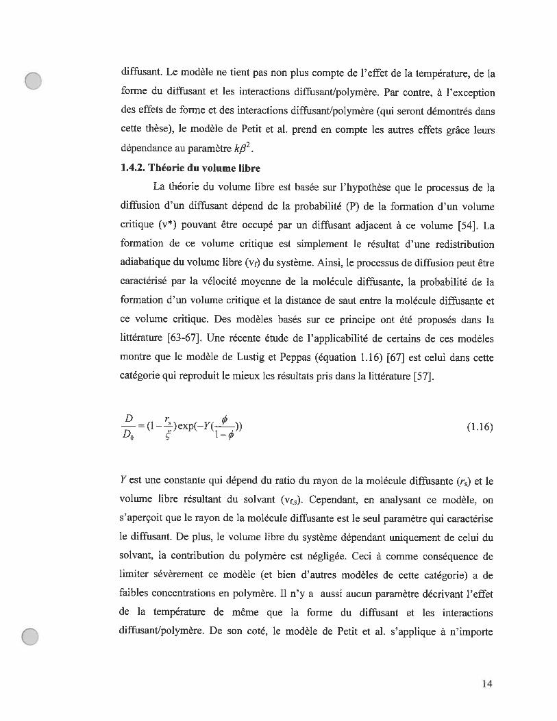
1.4.2. Théorie du volume libre

La théorie du volume libre est basée sur l’hypothèse que le processus de la

diffusion d’un diffusant dépend de la probabilité (P) de la formation d’un volume

critique (v*) pouvant être occupé par un diffusant adjacent à ce volume t54]. La

formation de ce volume critique est simplement le résultat d’une redistribution

adiabatique du volume libre (vf) du système. Ainsi, le processus de diffusion peut être

caractérisé par la vélocité moyenne de la molécule diffusante, la probabilité de la

formation d’un volume critique et la distance de saut entre la molécule diffusante et

ce volume critique. Des modèles basés sur ce principe ont été proposés dans la

littérature [63-67]. Une récente étude de l’applicabilité de certains de ces modèles

montre que le modèle de Lustig et Peppas (équation 1.16) [67] est celui dans cette

catégorie qui reproduit le mieux les résultats pris dans la littérature [57].

(1.16)

Y est une constante qui dépend du ratio du rayon de la molécule diffusante (ra) et le

volume libre résultant du solvant (v). Cependant, en analysant ce modèle, on

s’aperçoit que le rayon de la molécule diffusante est le seul paramètre qui caractérise

le diffusant. De plus, le volume libre du système dépendant uniquement de celui du

solvant, la contribution du polymère est négligée. Ceci à comme conséquence de

limiter sévèrement ce modèle (et bien d’autres modèles de cette catégorie) a de

faibles concentrations en polymère. Il n’y a aussi aucun paramètre décrivant l’effet

de la température de même que la forme du diffusant et les interactions

diffusant/polymère. De son coté, le modèle de Petit et al. s’applique à n’importe

14

Qquelle concentration en polymère. En comparant ce modèle à celui de Petit et al., on

arrive à la conclusion précédente.

1.4.3. Théorie d’obstruction

Dans la théorie d’obstruction, la chaîne de polymère est présentée comme une

structure immobile (relativement au diffusant et au solvant) et totalement

imperméable à la diffusion. Cette condition limite conduit à une augmentation du

libre parcours moyen du diffusant entre deux points du système. Cette définition du

processus de diffusion a conduit à plusieurs modèles essentiellement adaptés à la

diffusion dans les solutions et les gels hétérogènes [57, 5$, 6$-71]. Récemment,

Amsden a proposé un nouveau modèle théorique décrivant la diffusion dans les

hydrogels homogènes [5$, 71]. Ce modèle considère que la diffusion d’une molécule

donnée dépend de la probabilité de formation d’un espace suffisant entre les chaînes.

Cet espace se produit grâce au mouvement thermique aléatoire des segments de

chaînes du polymère. Plusieurs expressions ont été proposées et chacune d’entre elles

prend en compte l’effet de la qualité du solvant sur tel que défini par $chaefer et

Han. L’expression générale de ce modèle est:

D t r+rS P )2 (1.17)

D0

r est le rayon de la chaîne polymère, r est le rayon de la molécule diffusante.

Lorsqu’on est dans un régime de solvant marginal, l’équation 1.17 prend la forme

suivante:

D r+r—=exp —,r( P )2 (1.1$)D0 KØ2+2r

avec an’ (1 — 2z)_1 et K est une constante d’échelle. Cependant, lorsqu’on est

dans un régime de solvant théta, Amsden propose l’équation 1.19:

15

C =exP[_t’2] (1.19)

avec K an2. L’applicabilité du modèle a été testée par diverses données de la

littérature et les résultats montrent que celui-ci décrit très bien l’influence de la

concentration en polymère et la taille du diffusant [58]. Cependant, il apparaît que le

rayon de la molécule diffusante est le seul paramètre qui décrit les effets dus aux

propriétés physico-chimiques de la molécule diffusante. Par exemple, aucun

paramètre ne permet de prendre en compte l’effet de la masse et de la forme du

diffusant, de même que les interactions diffusantlpolymère. Sachant que le rayon

d’une molécule varie peu avec la température, il apparaît aussi que le modèle ne

prend pas en compte l’effet de la température sur la diffusion d’une molécule donnée.

Par ailleurs, la variation de en fonction de la qualité du solvant est pris en compte

par ce modèle ce qui évite de faire l’approximation effectué par Petit et al. dans leur

modèle. De plus, la prise en compte de la qualité du solvant procure une description

plus juste de la matrice polymère.

1.4.4. Modèles combinés

Dans les modèles combinés, on propose une vision du processus de la

diffusion qui combine les grandes catégories présentées ci-dessus. L’idée d’un tel

processus de diffusion est fort probable et même plus juste. Cependant, la question

qui s’impose est : comment peut-on déterminer la contribution de chaque catégorie

par rapport au processus global? Parmi les quelques modèles proposés, aucun n’est

adapté aux matrices polymères homogènes [72, 73].

1.5. Techniques RI’IN utilisées

Plusieurs techniques permettent d’étudier le processus de diffusion, les plus

importants étant la fluorescence, la diffusion de la lumière en mode dynamique, le

traceur radioactif et la résonance magnétique nucléaire (RMN) [74-79]. Nous avons

choisi d’utiliser la RMN car, contrairement à la fluorescence, elle ne requiert pas que

la molécule d’intérêt fluoresce. Elle ne nécessite aucune préparation fastidieuse de

l’échantillon et elle n’est pas limitée par la concentration du milieu contrairement à la

16

diffusion de la lumière en mode dynamique. A l’opposé de la technique de traceur

radioactif, les mesures du coefficient d’auto-diffusion effectuées par RIvN ne

consomment pas beaucoup de temps. De plus, la RMN permet d’étudier le processus

de la diffusion de plusieurs diffusants simultanément (en absence de recouvrement de

signaux RMN). Néanmoins, lorsqu’il y a recouvrement de signaux, il est possible de

déterminer assez précisément chaque coefficient de diffusion si ceux-ci sont séparés

par plus de deux ordres de grandeurs. En plus de ces avantages, les avancées

technologiques des dernières années (la disponibilité des techniques de diffusion

multi-quanta et l’augmentation de la puissance des gradients de champ magnétique

appliqués (gradients supérieurs à 1000 GIcm)) rendent accessible l’étude de la

diffusion de diffusant tels que les macromolécules de masse molaire élevée.

Cependant, pour les résultats présentés dans cette thèse, nous avons utilisé deux

techniques RMN classiques de gradient de champ pulsé (RMN PFG). Ces techniques

sont l’écho de spin à gradient de champ pulsé [$0] et l’écho stimulé [$1]. La Figure

1.4 illustre la séquence d’impulsion de chacune des deux techniques. Une description

détaillée de chaque séquence est proposée dans l’annexe A (pages 169-177).

Cependant, on peut faire une description simplifiée des deux séquences en disant que

la série d’impulsions de radiofréquence (r.f.) de 90° et de 180° appliquée dans une

direction donnée (l’axe x ou l’axe y) permet d’éliminer la contribution due à

l’inhomogénéité du champ magnétique au signal d’écho observé après 2t1 (écho de

spin) et 2t1 +t2 (écho stimulé). L’ application de gradients de champ magnétique crée

un déphasage des spins (module la position des spins). Lorsqu’il y a de la diffusion,

cette application de gradients conduit à une diminution de l’intensité du signal d’écho

en fonction de la puissant (G) ou de la durée d’application (6) de ces gradients.

Cependant, cette diminution n’est pas uniquement due à la diffusion, elle est aussi

due aux processus de relaxation. Ainsi, pour garder constante la contribution des

phénomènes de relaxation les temps t1 oulet t2 doivent rester constants en fonction de

G ou de 6 La détermination de la valeur du coefficient d’auto-diffusion par chacune

des deux méthodes s’effectue respectivement selon les deux principales équations ci

dessous (l’équation 1.20 pour la méthode d’écho de spin et l’équation 1.21 pour la

(J méthode d’écho stimulé). Les deux expressions illustrent la variation de l’atténuation

17

Gdu signal RMN (ho) obtenue en fonction de la puissance (G) et de la durée

d’application (5) du gradient de champ magnétique (voir pages 173 et 174 de

l’annexe A):

a

r.f.

b

t’

I t2 2tln—= ———-——1n2—7262G2D(A—613)

T T,

t’

(1.20)

(1.21)

H ‘I90 fl 180v fl

Ii

t1 t2 t1

H

r.f.

90 fl 90

H LJ HA

90 flH +

Figure 1.4. Séquences d’impulsions de la technique RMN à gradient de champ pulsé.

(a) Séquence d’écho de spin et (b) séquence d’écho stimulé.

lnL = _L— y262G2D(A —5/3)

o

Dans ces deux équations jo et I sont les intensités respectives du signal en absence de

gradient de champ magnétique, T1 et T2 sont les temps respectifs de relaxation spin

réseau et spin-spin (voir pages 163-169 de l’annexe A), yest le ratio gyromagnétique

1$

du noyau observé (proton dans notre cas), D est le coefficient d’auto-diffusion et A

représente le délai entre les deux impulsions de gradient. ti et t2 sont des délais entre

l’application de deux impulsions radiofréquence. Pour garder constant l’effet de la

relaxations (T1 et T2) illustrée par les équations 1.20 et 1.21, les temps t1 et t2 restent

constants durant l’expérience.

Des techniques topographiques (imagerie RIvIN) ont été utilisées pour

caractériser la diffusion de l’eau à l’intérieur des comprimés et le processus de

gonflement de ces comprimés (voir pages 186-188 de l’annexe A). Généralement, les

techniques les plus couramment utilisées pour caractériser ce genre de système sont:

la gravimétrie [82], la chromatographie liquide à haute performance (HPLC) [$3, 84],

le simulateur du système gastrique Us? 24 [831, la microscopie à contraste de phase

[85, $6], la microscopie électronique à balayage [87]. Le désavantage de certaines de

ces techniques est qu’ elles ne permettent pas de caractériser simultanément la matrice

polymère et la molécule active. Par exemple, la gravimétrie permet d’étudier la

cinétique de pénétration du solvant (ou n’importe quelle solution simulant le liquide

biologique) à l’intérieur du comprimé mais aucune information n’est obtenue sur le

principe actif. Cependant, l’analyse périodique par HPLC du solvant permet de

déterminer la constante de vitesse du relargage ou le coefficient de diffusion de la

molécule active. Ces techniques ne permettent pas de voir comment le système se

comporte lorsque le solvant diffuse à l’intérieur du comprimé. C’est principalement

pour cette raison que l’imagerie RMN est devenue l’outil de choix pour étudier les

systèmes de libération contrôlée tels que les comprimés. Par exemple dans le cas d’un

comprimé, l’imagerie RMN permet de suivre et de quantifier à plusieurs endroits

simultanément la pénétration d’un solvant à l’intérieur du comprimé, ce qui n’est pas

faisable avec d’autres techniques topographiques. Le grand désavantage de la RMN

est sa faible sensibilité en comparaison à une technique telle que la fluorescence.

Cependant, dans les cas des études présentées dans cette thèse, nous n’avons pas eu à

faire face à des problèmes de cette nature.

1.6. Travaux antérieurs

Au cours de travaux antérieurs, nous avons étudié le processus de diffusion

dans les systèmes polymères des diffusants tels que:

19

O. les petites molécules (exemple le méthanol et le t-butanol)

• les oligo-éthylènes glycols avec ou sans groupements terminaux

(généralement des groupements aikyles)

• les poly(éthylène glycol)s

• les éthers de couronne

Différents facteurs influençant le processus de diffusion de ces molécules ont été

caractérisés en utilisant les techniques de RIv1N PFG décrites précédemment (voir

section : techniques RMN les page 16-18). Parmi les facteurs étudiés, on trouve

l’étude de l’influence de la masse molaire et de la taille de la molécule diffusante. Les

effets des groupes terminaux, de même que ceux de la concentration en polymère et

de la température ont aussi été étudiés [44, 48-50]. L’effet de la masse molaire du

polymère sur le processus d’auto-diffusion a été également abordé [$8]. Les résultats

obtenus ont permis de démontrer qu’à l’exception de la masse molaire du polymère,

tous les autres facteurs avaient une influence sur le processus de diffusion. L’absence

d’effets de la masse molaire s’explique par la faible taille du diffusant étudié (rayon

hydrodynamique d’environ 1.25 nm). En effet, il a été démontré par Bu et al. [89] et

funikawa et al. [90] que la masse molaire du polymère affecte le processus d’auto-

diffusion lorsque le diamètre des diffusants est supérieur à 25 nm. Les plus

importants modèles théoriques des trois catégories citées précédemment (les modèles

basés sur l’effet d’obstruction, l’effet hydrodynamique et la théorie du volume libre)

ont été utilisés pour une analyse plus judicieuse des résultats et aussi pour tester leur

domaine d’applicabilité. Les résultats expérimentaux ont aussi permis de développer

le modèle théorique de Petit et al. [44]. 11 a été démontré que le modèle de Petit et al.

était capable de très bien reproduire l’influence des facteurs cités précédemment (voir

la page 9) contrairement à certains modèles importants tels que le modèle de Macide

Meares [50] et le modèle de Ogston et al. [$8]. L’analyse des données expérimentales

a démontré que les paramètres du modèle avait un sens physique.

1.7. Objectifs de ce travail

L’ effet de la taille du diffusant observé dans les travaux antérieurs ne se limite

pas uniquement aux facteurs de la masse molaire et de la dimension de la molécule

diffusante mais est aussi relié à la forme du diffusant (le diffusant peut être sphérique,

20

Figure 1.5. Structure de deux dendrimères de poly(propylène imine) contenant des

groupements terminaux de triéthylèneoxy méthyle éther (PPI(TEO) où x = 8, 32).

D : segment dendritique

L13: segment linéaire 1,3

L14: segment linéaire 1,4

T : segment terminal

cylindrique, etc.). Dans le but de découvrir comment ce facteur de la forme du

diffusant affecte le processus de diffusion, nous avons entrepris ce travail. Nous

avons sélectionné un certain nombre de diffusants polymères tels que les polymères

dendritiques, les polymères hyperbranchés et les polymères linéaires. Les Figures 1.5

et 1.6 montrent la structure chimique de certains des polymères sélectionnés.

o

o

PPI(TEO)8 PPI(TEO)32

figure 1.6. Structure des polymères hyperbranchés de polyglycidols (HBPGs).

21

Tel que mentionné au début de ce chapitre, la mise en oeuvre de systèmes de

relargage contrôlé nécessite une compréhension et une maîtrise des facteurs affectant

la diffusion du principe actif à travers ces systèmes jusqu’à la cible. Ainsi, l’étude de

l’influence de la forme du diffusant sur le processus de diffusion contribuera à une

meilleure compréhension de ces systèmes. L’un des objectifs de cette étude a été de

voir comment, dans un contexte de l’effet de la forme du diffusant, les facteurs tels

que la concentration en polymère, la température, la masse molaire du diffusant

influençaient le processus de la diffusion. Nous voulons aussi tester la capacité du

modèle de Petit et al. à reproduire l’effet de la forme du diffusant. Pour cette étude,

l’alcool polyvinylique (PVA) a été choisi comme matrice polymère. Le PVA est

obtenu à la suite de l’hydrolyse du poly(acétate vinylique) (voir figure 1.7).

Hydrolyse

Alcool polyvinylique (PVA)

Figure 1.7. Structures chimiques de la préparation de l’alcool polyvinylique.

Selon le degré d’hydrolyse (DH) obtenu, le PVA peut être soluble dans l’eau à 25°C

(pour DH 80%), tandis que le même polymère ne se solubilise dans l’eau qu’à plus

de 90°C lorsque DH 95%. Le PVA est un polymère dont les propriétés physico

chimiques sont très bien documentées. C’est un polymère capable de former des

hydrogels physiques (enchevêtrement des chaînes) et des hydrogels chimiques

(réticulation avec un agent réticulant tel que le glutaraldéhyde).

Nous avons aussi fixé comme objectif d’étudier l’effet des interactions entre

des petites molécules diffusantes et diverses matrices polymères. La figure 1.8

montre les trois autres matrices utilisées pour cette étude des interaction

n

Poly(acétate vinylique) (PVAc)

n

Q:

22

diffusants/polymères. Tout comme l’effet de la forme, l’effet des interactions

diffusants/polymères est peu étudié. Cependant, ce facteur peut jouer un rôle

déterminant dans le processus de diffusion. L’ensemble des résultats de ces études

servira à tester les limites des modèles de Petit et al. et de Phillies [61, 62] pour ce

qui à trait à la capacité de ces deux modèles à prendre en compte des interactions

diffusant/polymère.

[ CH2—CH-3— [ CH2—CH+ [ CH2—CH+

COOH CH2 O=c

NH2

Poly(acide acrylique) (PAA) Poly(allylamine) (PAAm) Poly(N,N-diethylacrylamide) (PDEA)

Figure 1.8. Structures chimiques des autres matrices polymères utilisés pour l’étude

du processus de diffusion dans les solutions et les hydrogels de polymères.

Le deuxième grand objectif du présent travail a été d’étudier le processus de

gonflement et le processus de diffusion de l’eau dans des comprimés d’amidon à

haute teneur en amylose (70% d’amylose et 30% d’amylopectine). La figure 1.9

illustre la structure chimique de ces deux polysaccharides qui composent l’amidon.

L’amylose est un polymère essentiellement linéaire (99 % de liaisons a (1-4) et 1 ¾

de liaisons Œ (1-6)), contenant entre 500 et 6000 unités de D-glucose [91]. L’amylose

est connu pour avoir une conformation hélicoïdale (couramment appelé le V

amylose) dans laquelle on trouve 6 D-glucoses par tour et un arrangement vers

l’extérieur des groupements hydrophiles alors que les groupements hydrophobes sont

tournés vers l’intérieur. Cette conformation hélicoïdale permet à l’amylose de

complexer des molécules hydrophobes (par exemple les chaînes alkyles des lipides).

Cependant, lorsque le polymère est hydraté, on observe un changement de la

conformation V-amylose vers une conformation double hélice (A-amylose, B

(Z’ amylose et C-amylose) [92-94]. Contrairement à la conformation V-amylose, les

23

doubles hélices A-, B- et C-amylose sont très compactes (elles ne peuvent complexer

de petites molécules) et l’arrangement des groupements hydrophobes et hydrophiles

est irrégulier. La double hélice est constituée de 2x6 D-glucoses par tour [95, 96].

L’amylopectine est un polymère ramifié dont la masse molaire varie entre 50

et 100 Millions. Les unités D-glucoses sont reliées entre elles par des liaisons a (1-4)

et ces dernières représentent environ 95 % des liens totaux entre les unités de D-

glucose [91]. Les 5 % des liaisons restantes sont de type Œ (l-6) et elles forment les

points de ramification [91]. L’amylopectine est généralement représenté comme un

ensemble de grappes de chaînes courtes (entre 15 à 25 unités de D-glucose) liées

entre elles par des chaînes plus longues (entre 40 à 60 unités de D-glucose) [91].

a

lien Œ (1-4)

figure 1.9. Structures chimiques de l’amylose ta) et de l’amylopectine (b).

lien a (1-4)

Amylose

b

lien Œ (1-4)

Amylopectine

24

Par rapport aux solutions et hydrogels des polymères précédents, ces comprimés

permettent de suivre le processus de diffusion dans une situation réelle d’un système

de relargage contrôlé. Pour cette étude, l’imagerie RMN a été utilisée car celle-ci est

parfaitement adaptée à cette situation. L’effet de la température et la taille des

comprimés sur le gonflement et la diffusion de l’eau ont été étudiés. L’ensemble des

études présentées dans ces deux grandes parties de la thèse a pour principal objectif

de mieux comprendre le processus de diffusion dans les systèmes polymères

permettant ainsi une meilleure applicabilité des matériaux polymères dans

l’élaboration de systèmes de libération contrôlée de principes actifs.

1.8. Présentation des travaux

Les travaux effectués et présentés dans cette thèse se divisent en deux grandes

parties. La première partie contient trois chapitres traitant du processus de diffusion

dans les solutions et les hydrogels de polymères. Dans le premier chapitre (chapitre

2) de cette première partie, il est question de la diffusion de dendrimères de

polyQropylène imine) contenant des groupements terminaux de triéthylèneoxy

méthyle éther (PPI(TEO)) dans des solutions et hydrogels de PVA. Les résultats

présentés dans ce chapitre débutent par une caractérisation par RMN (assignation des

spectres RMN du proton et détermination de la masse molaire) des dendrimères,

suivie d’une étude des phénomènes de relaxation (temps de relaxation spin-réseau ou

T1 et temps de relaxation spin-spin ou T2) des différents segments de chaque

dendrimère. Le reste du chapitre est consacré aux études de l’effet de la masse

molaire du diffusant, de l’effet de la concentration de PVA et de l’effet de la

température sur le processus de l’auto-diffusion. Les données expérimentales ont été

traitées avec le modèle de Petit et al.. Les paramètres du modèle ont été corrélés avec

les rayons hydrodynamiques (Rh) des diffusants. Ces rayons hydrodynamiques et les

coefficients d’auto-diffusion en absence du polymère (D0) ont été corrélés avec la

masse molaire afin de déterminer qualitativement le type de distribution de densité de

ces dendrimères. L’effet de la température sur cette distribution de densité a été aussi

illustré. Nous avons aussi comparé, sur le plan de l’énergie d’activation apparente, les

dendrimères et les poly(éthylène glycol)s (PEGs).

25

Dans le deuxième chapitre (chapitre 3), nous nous sommes intéressés au

processus de la diffusion des polymères hyperbranchés de polyglycidols (HBPGs).

Les mêmes effets que ceux étudiés dans le chapitre précédent ont été étudiés. Les

résultats obtenus ont permis de démontrer clairement l’effet de la forme du diffusant

sur le processus d’auto-diffusion. Pour cette illustration, la comparaison entre les

valeurs du coefficient d’auto-diffusion des polymères dendritiques, des polymères

hyperbranchés et des polymères linéaires de masses molaires similaires a été

effectuée. Pour cette comparaison les études ont été effectuées dans des conditions

expérimentales identiques. À la suite de la démonstration de l’effet de la forme, ces

résultats ont été utilisés pour tester la capacité du modèle de Petit et al. à prendre en

compte cet effet de la forme.

Le troisième chapitre (chapitre 4) porte sur l’étude de l’effet des interactions

spécifiques (par exemple les liaisons hydrogène) entre le diffusant et la matrice

polymère. Ce chapitre inclut l’étude de l’effet des groupes fonctionnels (groupements

alcoolique, amine et acide carboxylique), des molécules diffusantes de même que

l’effet des groupes fonctionnels en position latérale sur la matrice polymère. Le

modèle de Petit et al. et celui de Phillies ont été utilisés afin de vérifier leur capacité à

prendre en compte l’influence des interactions spécifiques sur le processus de

diffusion.

Dans la deuxième partie de cette thèse, nous nous sommes intéressés à

l’étude par imagerie RMN de la diffusion de l’eau à l’intérieur des comprimés

d’amylose. Nous avons caractérisé le processus de gonflement qui se produit lors du

mouillage (pénétration de l’eau à l’intérieur des comprimés). L’ensemble des travaux

de cette partie se présente sous forme de deux chapitres. Le premier chapitre (chapitre

5) traite de l’effet de la température sur le processus de la diffusion de l’eau de même

que son influence sur le processus de gonflement. Des valeurs de coefficient de

diffusion, de vélocité et de constante de vitesse de gonflement ont été déterminées.

Dans le second chapitre (chapitre 6), nous avons examiné l’effet de la taille des

comprimés sur les processus de la diffusion et du gonflement de même que la

diffusion anisotrope selon l’axe de compression. Des études de thermogravimétrie

ont aussi été effectuées et les résultats ont été comparés à ceux obtenus par imagerie

26

RIVIN. Des valeurs de coefficient de diffusion, de vélocité et de constante de vitesse

de gonflement sont aussi présentées.

1.9. Références

[1] Nabi Saheb, D.; Jog, J. P. Adv. Folym. Tech. 1999, 18, 351-363.

[2] Gil, M.; Ji, X.; Li, X.; Na, H.; Hampsey, J. E. ; Lu, Y. I Membr. Sci. 2004,

234, 75-81.

[3] Kavuklu, Ô.; Gûner, A.; Tunoglu, N. Adv. PoÏym. Tech. 2002, 21, 125-13 1.

[4] Wang, Z.-L.; Tang, Z.-Y. Electrochim. Acta 2004, 49, 1063-1062.

[5] Tharanathan, R. N. Trends FoodSci. Tech. 2003, 14, 71-78.

[6] Dodane, V.; Vilivalam, V. Fharm. Sci. Technol. 1998, 1, 246-253.

[7] Ilium, L. Pharm. Res. 1998, 15, 1326-133 1.

[8] Yuqing, M.; Jianrong, C.; Xiaohua, W. Trends Biotechnol. 2004, 22, 227-231.

[9] Saxena, V.; Maihotra, B. D. Curr. Appi. Phys. 2003, 3, 293-305.

[10] Breitenkamp, R. B.; Tew, G. N. Macromolecules 2004, 37, 1163-1165.

[11] Jeong, B.; Gutowska, A. TrendsBiotechnoÏ. 2002, 20, 305-311.

[12] Compton, R. A. Long-term Effect Med Implants 1997, 7, 29-54.

[13] Jagur-Grodzinski, J. React. Funct. Polym. 1999, 39, 99-138.

[14] Phaneuf, M. D.; $zycher, M.; Berceli, S. A.; Dempsey, D. J.; Quist, W. C.;

LoGerfo, f. W. Artf Organs 1998, 22, 65 7-665.

[15] Hirano, S. Biotechnol. Annu. Rev. 1996, 2, 237-258.

[161 Liggins, R. T.; Burt, H. M. Adv. Drug Deliv. Rev. 2002, 54, 19 1-202.

[17] Lele, B. S.; Leroux, J. C. Macromolecules 2002, 35, 67 14-6723.

[18] Lavasanifar, A.; Samuei, J.; Kwon, G. S. Adv. Drug Deliv. Rev. 2002, 54,

169-190.

[19] Zuleger, S.; Fassihi, R.; Lippold, B. C. Int. I Pharm. 2002, 247, 23-37.

27

G[201 Kydonieus. A. F. ControÏled Release Technologies: Methods, Theory and

Applications, Vol. 1, Marcel Dekker, USA, 1980.

t21] Bhattacharya, R.; Phaniraj, T. N.; Shailaja, D. J Membr. Sci. 2003, 227, 23-

37.

[221 Kost, J.; Horbert. T. A.; Ratner, B. D.; et al. J Biomed. Mater. Res. 1985, 19,

117-1133.

[23] Heller, J.; Pangbum, S. H.; Penhale, D. W. H. Use ofBioerodible Polymers in

SefRegulated Drug Delivery Systems, Controlled-Release Technology,

Pharmaceutical Applications, Lee PI and Good WE editors, Washington DC,

ACS Symposium Series, 1987, p. 172-187.

[24] Dorski, C. M.; Doyle, F. J.; Peppas, N. A. Polym. Mater. Sci. Eng. Proceed

1997, 76, 281-282.

[25] Jeong, B.; Bae. Y. H.; Kim, S. W. J Control. Release 2000, 63, 155-163

[26] Jeong, B.; Choi, Y. K.; Bae, Y. H.; Zentner. G.; Kim, S. W. J Control.

Release 1999, 62, 109-1 14.

[27] Torres-Lugo, M.; Peppas, N. A. Macromolecules 1999, 32, 6646-6651.

[2$] Tang M. X.; Redemann C. T.; Szoka f. C. Bioconjugate Chem. 1996, 7, 703-

714.

[29] Cappello, J.; Crissman, J. W.; Crissman, M.; Ferrari, f. A.; Textor, G.;

Wallis, O.; Whitledge, J. R.; Zhou, X.; Burman, D.; Aukerman, L.;

Stedronsky, E. R. J Control. Release 1998, 53, 105-117.

[301 Gazzaniga. A.; Sangalli, M. E. Ettr. J Pharm. Biopharm. 1994, 10, 246-250.

[31] Ma, J.; Feng. P.; Ye, C.; Wang, Y.; Fan. Y. ColloicL Polym. Sci. 2001, 279,

387-392.

[32] Suzuki, Y.; Tanihara, M.; Nishimura, Y.; Suzuki, K.; Kakimani. Y.; Shimizu,

Y. J Biomed Mater. Res. 1998, 42, 112-116.

[33] Seal, B. L.; Panitch, A. Biomacromolecules 2003, 1, 1572-1582.

28

[34] Voet, D.; Voet, J. G. Biochemistry 2nd ed., John Wiley & Sons, N.Y., 1995.

[35] Crank, J. The Mathematics of Diffusion 2’ ed., Clarendon Press, Oxford

1975.

[36] Crank, J.; Park, G. S. Diffusion in Polymers 1st ed., Academic Press, New

York 1968.

[37] Cussler, E. L. Diffusion Mass Transfer in Fluid Systems, 2’ ed., Cambridge

University Press, 1997.

[3$] Masaro, L; X. X. ZhuProg. Polym. Sel. 1999, 24, 73 1-775.

[39] Alftey Jr., T.; Gumee, E. f.; Lloyd, W. G. J PoÏym. Sci. Part C 1966, 12,

249-257.

[40] Grinsted, R. A.; Clark, L.; Koenig, J. L. Macromolecules 1992, 25, 1235-

1241.

[41] Lewis, C. M.; Mutsears, P. H. A.; de Jong, A. M.; van Ijzendoom, L. J.; de

Voigt, M. J. A.; Ren, M. Q.; Watt, F.; Broer, D. J. J Chem. Phys. 2004, 120,

1820-1825.

[42] Cohen, M. H. and Tumbuil, D. J Chem. Phys. 1959, 31, 1164-1169.

[43] Turner, D. N.; Hallet, f. R.; Biochim. Biophys. Acta 1976, 451, 305-3 12.

[44] Petit, J.-M.; Roux, B.; Zhu, X. X.; Macdonald, P. M. Macromolecules 1996,

29, 603 1-6036.

[45] De Gennes, P. G. Scaling Concepts in Polymer Physics; Comeli University

Press: Ithaca, NY, 1979.

[46] Macey, R.I. Membrane Physiology, Andreoli, T.E., Hoffman, J.f., and

Fanestil, D.D., Ed.; Plenum Press, New-York, 1980, Chap. 7.

[47] Kramers, H. A. Physica 1950, 7, 248-255.

[4$] Schaefer, D. W.; Han, C. C. Dynamic Light Scattering and Velocimetry:

Applications of Photon Correlation Spectroscopy Pecora, R., Ed., Plenum

Press, New York, 1982, Chap. 5.

29

[49] Schaefer, D. W. Potymer 1984, 25, 387-394.

[50] Masaro, L.; Zhu, X. X.; Macdonald, P.M. MacromoÏecules 1998, 31, 3880-

3885.

[51] Masaro, L.; Zhu, X. X. Macromolecules 1999, 32, 5383-5390.

[52] Masaro, L.; Zhu, X. X.; Macdonald, P.M. I Polym. Sci.. Part B: Polym.

Phys. 1999, 37, 2396-2403.

[53] Fujita, H. Adv. PoÏym. Sci. 1961, 3, 1-47.

[54] Yasuda, H.; Lamaze, C. E.; Ikenberry, L. D. Makromol. Chem. 1968, 118, 19-

35.

[55] Phillies, G. D. J. Macromolecules 1986, 19, 2367-2376.

[56] Vrentas, J. S.; Vrentas, C. M. Macromolecules 1994, 27, 4684-4690.

[57] Amsden, B. Macromolecules 1998, 31, 8382-8395.

[58] Amsden, B. Polymer 2002, 43, 1623-1630.

[59] Cukier, R. I. Macromolecules 1984, 17, 252-255.

[60] Altenberger, A. R.; Tirreil, M.; Dahier, J. S. I Chem. Phys. 1986, 84, 5 122-

5130.



[63] fujita, H. Adv. Polym. Sel. 1961, 3, 1-47

[64] Yasuda, H.; Lamaze, C. E.; Ikenberry, L. D. Die Makro. Chem. 1968, 118,

19-25.

[65] Vrentas, J. S.; Duda, J. L. I Polym. Sci, Polym. Phys. EL 1977, 15, 403-4 16.

[66] Peppas, N. A.; Reinhart, C. T. I Membr. Sci. 1983, 15, 275-283.

[67] Peppas, N. A.; Lustig, S. R. Hydrogels in Medecine and Pharmacy, Vol. I,

CRC Press, Boca Raton, 1987, p. 57.

[68] fricke, H. Phys. Rev. 1924, 24, 575-587.

30

[69] Mackie, J. S.; Meares, P. Froc. R. Soc. Lond A 1955, 232, 510-518.

[70] Ogston, A. G.; Preston, B. N.; Wells, J. D. Froc. R. Soc. Lond, A 1973. 333,

297-316.

[71] Amsden, B. Macromolecules 1999, 32, $74-879.

[72] Johnson, E. M.; Berk, D. A.; Jain, R. K.; Deen, W. M. J Biophys. 1996, 70,

1017-1023.

[73] Clague. D. S.; Phillips. R. J. Phys. fluids 1996, 8, 1720-173 1.

[74] Westrin, B. A.; Axelson, A.; Zacchi, G. J Contr. Release 1994, 30, 189-199.

[75] Hu, D. S.-G.; Chou, K. J.-N. Folymer 1996, 37, 10 19-1025.

[76] Smith, B. A. H.; Sefion, M. V., I Biomed Mater. Res. 1988, 22, 673-685.

[77] Wisnudel, M. B.; Torkelson, J. M. Macromolecules 1996, 29, 6 193-6207.

[72] Kosmeyer, R. W.; Peppas, N. A. J Membr. Sci. 1981, 9, 211-227.

[79] van Asten, A. C.; Kok, W. T.; Tiissen R.; Poppe, H. I Folym. $cï.: Fart B

Folym. Fhys. 1996, 34, 283-295.

[80] Stejskal, E.O.; Tanner, I.E. I Chem. Fhys. 1965. 42, 228-292.

[81] Tanner, J. E. J Chem. Fhys. 1970, 52, 2523-2526.

[82] Moussa, I. S.; Cartilier, L. H. J Control. Release 1996, 42, 47-55.

[83] Sangalli, M. E.; Maroni, A.; Zema, L.; Busetti, C.; Giordano, f.; Gazzaniga,

A.J Confrol. Release 2001, 73. 103-110.

[84] Miyajima, M.; Koshika, A.; Okada, J.; Ikeda, M. I Control. Release 1999,

6], 295-304.

[85] fleming, A. B.; $altzman, W. M. J Control. Release 2001, 70, 29-36.

[86] Ahmed, f.; Discher, D. E. J Control. Release 2004, 96, 37-53.

[$7] Zhang, K.; Wu, X. Y. Biomaterials 2004, 25, 528 1-5291.

[88] Masaro, L.; Ousalem, M.; Baille, W. E.; Lessard, D.; Zhu, X. X.

Macromolecules 1999, 32, 4375-4382.

nj

[$9] Bu, Z.; Russo, P. S.; Macromolecules 1994, 27, 1187-1194.

[90] furukawa, R.; Arauz-Lara, J. L.; Ware, B. R. Macromolecules 1991, 24, 599-

605.

[91] Immel, S.; Lichtenthaler, F. W. $tarch/$t&rke 2000, 52, 1-9.

[92] Shifian, D.; Ravenelle, F.; Mateescu, M.A.; Marchessault, R.H. StarcW$tarke

2000, 52, 186-195.

[93] Moussa, I.S.; Cartilier, LII. I Control. Release 1996, 42, 47-52.

[94] Ravanelle, F.; Marchessault, R.; Légaré, A.; Buschmann, M.D.; CarbohycL

Folym. 2001, 47, 259-264.

[95] Veregin, R. P.; Fyfe, C. A.; Marchessault, R. H. Macromolecules 1987, 20,

3007-3012.

[96] Brisson, J.; Chanzy, H.; Winter, W. T. bit. I Biol. Macromol. 1991, 13, 31-

39.

o32

o

Chapitre 2

Self-Diffusion of Hydrophulic

Poly(propyleneimine) Dendrimers in Poly(vinyl

alcohol) Solutions and Gels by Pulsed Field

Gradient NMR Spectroscopy

W. E. Baille, C. Malveau, X. X. Zhu, Y. H. Kim, W. T. Ford

MacrornoÏecules 2003. 36, 839-847

o

2.1. Abstract

Pulsed-field gradient NMR spectroscopy was used to study the diffusion of

three different po1yQropy1eneimine) dendrimers with hydrophilic triethylenoxy

methyl ether terminal groups (generations 2, 4 and 5) in poly(vinyl alcohol) aqueous

solutions and gels. The effects of the diffusant size, polymer concentration (from O to

0.26 g/mL) and temperature on the self-diffusion coefficients have been studied and

the model of Petit et al. [Macromolecutes, 1996, 29, 6031] was used to fit the

experimental data. The Stokes-Einstein hard-sphere radii were also caÏculated in the

zero concentration limit and were compared with those of the linear poly(ethylene

glycol)s under the same conditions. The proton NMR relaxation times (T1 and T2)

were measured to study the mobility of the dendrimer core part and terminal group as

a function ofthe dendrimer size.

o34

2.2. Introduction

The diffusion of various solute molecules in polymer solutions and gels is

very important in the application of polymer solutions and gels. Examples include

permeation through polymer membranes [1], diffusion of piasticizers in plastic

materials [2], and drug release from polymer gels [3]. The study of self-diffusion of

different solutes and additives in polymers may help in the elucidation of the effects

of polymer concentration, size and shape of the diffusant, temperature and specific

interactions within the polymer network [4]. The information is critical in

determining the applicability of polymeric materials in industry. Various physicai

models of diffusion have been proposed over the years [5-13]. These physical modeis

cf diffusion are essential for the interpretation of the resuits. Pulsed field gradient

(PFG) NMR techniques have been used successfully in the study of self-diffusion of

solute and soivent moiecuies in polymer solutions and gels [4, 11, 14-24].

We have previously studied the self-diffusion in polymer solutions and gels of

solute molecules ranging from small molecules to polymers [4, 11, 25-28]. The

resuits obtained by the study of the diffusion of small diffusants with different

functionai groups (alcohol, amine, ammonium sait, amide and acid) in poiy(vinyi

alcohol) (PVA) solutions and gels show that the diffusion behavior is primarily

influenced by the size of the diffusant and secondarily by the chemical interactions

[25]. for the self-diffusion of iinear oligo- and poiy(ethylene glycol)s (PEGs) the

moiecuiar size of the diffusant plays the most important part in the diffusion process

[4, 25, 27]. The effect of the polymer matrices on the self-diffusion cf PEG with

molecular weight 600 was aise studied for different ternary polymer-water-PEG

systems [26]. The diffusion cf the PEG did not vary significantly with the molecular

weight cf the PVA matrix and only a small variation was observed with the degree cf

hydrolysis of the PVA. The diffusion in hydrophiiic polymers is mostly affected by

formation of the hydrogen bonds between the solute and the polymer matrix. Ah

these studies have aiiowed us to test the applicability cf a new physical mode!

developed by our group [11]. This model has been used successfuliy to describe the

effect of the poiymer concentration, the temperature and the diffusant size on the

(J’ diffusion process in polymer gels.

35

The PEG diffusants used in our smdies so far differed in their molecular

weights [4, 27] and sometimes in their chain-end groups [2$], but they are ail linear

polymers. A hydrodynamic radius can be estimated for such molecules in solution,

but the exact process of diffusion of these linear oligomers and polymers in a gel

matrix remains to be clarified. In addition, there is a problem ofpolydispersity ofthe

PEG samples even after fractionation. It would be interesting to compare their

behavior with that of more spherical molecules with similar molecuiar weights but

different sizes of the cross-sections. Dendritic polymers are molecules of choice

because of the good control in their molecular size and shape (more spherical).

Moreover, dendritic polymers have a more regular conformation and a lower degree

of polydispersity in comparison to highly branched polymers [29-32]. These

characteristics make dendrimers very interesting and useful as a model diffusion

probes. Also, they cari be used in many different applications such as molecular

encapsulation for drug delivery, membrane transport or molecular recognition [33,

34]. Therefore, the self-diffusion process of three different polyQropylene- imine)

(PPI) dendrimers with hydrophilic triethylenoxy methyl ether (TEO) terminal groups

in PVA aqueous solutions and gels was studied by the PFG NMR technique. The

effects of polymer concentration, temperature and dendrimer size on the self-

diffusion coefficients were investigated. We have also studied the mobility of the

dendrimer core part and terminal group as a function of generation by the

measurement of ‘H NMR relaxation times (T, and T2).

2.3. Experimental Section

2.3.1. Materials

DAB-dendr-(NH2) (n = 8, 32, and 64) and ah other chemicals were

purchased from Aldrich (Milwaukee, WI). Triethylamine (TEA) was dried over

anhydrous 3 À molecular sieves and freshly distilled. Ail other chemicals were used

as received. D20 was purchased from C.I.L. (Andover, MA).

2.3.2. 2-[2-(2-Methoxyethoxy)ethoxyjacetyl Chloride

A solution of 2-[2-(2-methoxyethoxy)ethoxy]acetic acid (5.34 g, 30.0 mmol)

and oxalyl cifioride (6.35 g, 50.0 mmoi) in 3 mL oftoluene was stirred for 4 h at 65

°C. The solvent and excess reagent were removed under reduced pressure, and the

36

residue was dried at 40 oc under vacuum to give a light yellow ou (5.34 g, 90%)

which was used without fiirther purification.

2.3.3. Modified Poly(propyleneimine) Dendrimers (35, 361

2-[2-(2-Methoxyethoxy)ethoxy]acetyl chloride (3.00 g, 15.3 mmol) was

added to a solution of PPI dendrimer DAB-dendr-(NH2)g (1.00 g, 1.29 mmol), DMf

(5.0 mL), and TEA (0.9 g. 8.89 mmol) at O °c. The solution was stirred under

nitrogen at 70 oc for 24 h. Water (5 mL) was added to hydrolyze the excess acid

cifioride. The mixture was made basic to pH > 14 using 5 g (27 mmol) of

tetramethylammonium hydroxide pentahydrate and was extracted with CH2C12 (4

times 10 mL). The combined dichioromethane solution was dried over Na2SO4 and

evaporated. The oily residue was dried at 40 °c under vacuum to give a light yellow

ou of PPI(TEO)s (2.21 g, 83%). DA3-dendr-(NH2) (n 32 and 64) were also

modified with triethylenoxy methyl ether end groups by the same procedure to yield

PPI(TEO)32 and PPI(TEO)64. The 1H and ‘3c NMR spectra of dendrimers made by a

slightly different procedure were the same as the spectra of those reported here [35,

36].

2.3.4. Sample Preparation

Samples were prepared following the method described previously [4, 11].

PVA (M = 52 000 with a degree of hydrolysis 99%) was added to a D20 solution

containing 1 wt % of dendrimer probes in 5 mm o.d. NMR tubes. The NMR tubes

were sealed to avoid solvent evaporation and heated at temperature between 100 and

110 °c to dissolve the PVA and to help in the mixing of the sample. The heating

helped also to prevent gelation effects. The concentration of PVA ranged ftom O to

0.26 g/mL.

2.3.5. Molecular Weight Determination

‘H NMR experiments were performed on a Bruker AMX-300 spectrometer

operating at a frequency of 300.13 MHz to determine the molecular weights (Ma) of

the dendrimer, based on the ratio of the integrated peak areas of the methylene

protons at 4.05 ppm to the methylene groups in the core.

2.3.6. Relaxation lime Measurements

‘H spin-lattice (T1) and spin-spin (T2) relaxation times were measured on a

37

Bruker AMX-300 spectrometer operating at 300.13 MHz. Experiments were

conducted at 25 °C. T1 was obtained with the classicai inversion-recovery pulse

sequences. Ail measurements were performed using eight scans with a repetition time

of 30 s. A total of 24 increments of the recovery time between 0.01 and 25 s were

used. The T1 values were extracted by the use of

= 1—kexj— (2.1)M0 TJ

where M0 and M are the magnetization at equilibrium and for a recovery time i

respectively, T1 and k can be calculated by least mean square method. The variable k

is ideally equal to 2 but for ail experiments k obtained are between 1.8 and 2.0. T2

measurements were performed with the classical carr-Purceil-Meiboom-Gill

(CPMG) pulse sequences. The T2 values were extracted ftom

M t 2rn”—=expi——-——i (2.2)M0 7J

where M0 and M are the magnetization at the equilibrium and at the nth echo,

respectively. y is a fixed echo time (set at 2 ms), which allows the attenuation of

diffusion and J-modulation effects, and n is an even number of echoes (32 values

between 2 and 2400 echoes were chosen).

2.3.7. Pulsed Field Gradient NMR Measurements

The selfdiffusion coefficient (D) measurements were performed using the

stimulated echo (STE: 90°-ti-90°-t2-90°-ti-echo) sequence deveioped by Tanner [37]

on a Bruker DSX-300 NMR spectrometer operating at a frequency of 300.18 MHz

for protons. A Bruker imaging probe (Micro2.5 probe) was used with a tbree

orthogonal field gradient cous system permitting a maximum gradient of 100 GIcm.

C The self-diffusion coefficients were obtained from the attenuation of the NMR

3$

signais due to the application of the gradient pulses of various strengths in a

stimuiated echo sequence, as given in the following expression [3 8-40]

in’ = __.L_ln2_y262G2D(A_6/3) (2.3)

where I and 1o are the NMR signal intensities in the presence and in the absence of

the gradient, respectively, ti is the interval between the first two 90° r.f. pulses and

between the third 90° r.f. pulse and the middie ofthe echo, t2 is the delay between the

second and the third 90° r.f. pulses, yis the gyromagnetic ratio of the nucleus under

observation, 6 and G are the duration and the strength of the applied gradient pulse,

respectively, D is the self-diffusion coefficient, and is the time interval between the

two successive gradient pulses (also calied the diffusion time). The self-diffusion

coefficient was extracted from the slopes of the unes obtained from linear regression

of the logarithm of signal intensity as a function of G2. Excellent linear relationships

have been obtained in these experiments with correlation coefficients of 0.996 and

better. The error of the measured D values was estimated to be 5% by carrying out

repeated experiments with selected samples.

The experiments were performed at different temperatures from 5 to 45 °C

(fluctuation of the temperature ± 0.3°C) and concentrations of PVA ranged from O to

0.26 g/mL. Temperature calibration was done periodically on the NMR instrument by

measuring the chemical shifi difference between the ‘H NMR signals of CH2 and OH

groups of pure ethylene glycol at various temperatures since this difference is

sensitive to temperature changes [41].

A nonlinear least-square fitting method was used in ah cases to fit the

experimental diffusion data to the model of Petit et al. [11] The correlation

coefficients r2 yieided were in the range 0.997 0.999. The quahity of the fitting to

the experimental data was also indicated by the good fits shown in all the figures.

The saine sets of fitting parameters were obtained regardless of the initial values used

in the procedure.

39

2.4. Resuits and Discussion

2.4.1. NMR Characterization

‘H NMR spectra of the synthesized products were done in D20 at 1 wt % of

the dendrimers. The reaction of the amine groups on the dendrimer surface with TEO

is evidenced by the high field shifi ofthe methylene protons from 4.75 ppm (for TEO

before reaction) to 4.05 ppm (peak labeled f in Figure 2.1). These spectra also

coiffirm the structure of dendrimers. Ail the proton signais of the dendrimers are

assigned (figure 2.1). The NMR spectra were also used to determine the molecular

weight of these dendrimers (Table 2.1). The molecular weight was obtained from the

integrated area ratio of methylene protons at 4.05 ppm (peak f) and methylene

protons at 1.73 ppm. The comparison between the values expected for an ideal

dendrimer growth and the values determined experimentally by ‘H NMR

spectroscopy allows the determination of the molecular weight. This ratio also helps

to determine the completeness of the end groups amidation. The experimental

intensity ratio obtained for each dendrimer generation show that the modified

polyQ,ropyleneimine) dendrimers synthesized are practically ideal.

Table 2.1. Some characteristics of the modified poly(propyleneimine)

dendrimers

number ofsamples terminal groups Ma (g/mol) Mb (g/mol)

generations

PPI(TEO)8

PPI(TEO)32

PPI(TEO)64

2

4

5

$

32

64

2055

$639

17396

(a)Molecujar weight calcuiated for ideal dendrimer growth.

(b)Numberaverage molecular weight determined by ‘H NMR spectroscopy.

2000

$600

17000

40

çJ

0,H H,

ONg

iÇh.j

H

a I N-

H

A c, d, e ON H

(

gi h

________/ \j - -

r L_C

4.5 4.0 3.5 3.0 2.5 2.0 1.5 1.0(ppm)

Figure 2.1. 1 H NMR spectra of three different poly(propyleneimine) dendrimers with

hydrophilic triethylenoxy methyl ether terminal groups at 1 wt% in D20 at 25 °C. (A)

PPI(TEO)s, (B) PPI(TEO)32, (C) PPI(TEO)64.

41

Q2.4.2. Relaxation Times Measurements

‘H NMR relaxation times (T, and T2) were measured to study the motions of

three different parts of the dendrimers (methyl and methylene protons of the terminal

groups and methylene protons of the core) as a function of generation. The results

obtained are listed in Table 2.2. Ail dendrimers showed a sharp decrease (ca. 50

times) in the T2 from the methyl protons of the terminal groups (peak a) to the

methylene protons of the core (peaks h and j). Moreover, a large difference is

observed among the three distinct zones. This resuit indicates that the mobility

increases from the inner core of the dendrimers to the outer part. Table 2.2 also

shows a decrease in T2 at higher generations of the dendrimers. A decrease by a

factor of ca. 2 was observed between the PPI(TEO)s and the PPT(TEO)64 for all

peaks, indicating a decrease in the mobiiity of the dendrimers. In the measurements

of ‘H T,, for the terminal groups a decrease in the T, was observed with increasing

dendrimer generation. but an increase in the T1 was observed for core protons.

Table 2.2. NMR relaxation times for the different 1H signais of the

dendrimers at 25 °C

NMR peaksasamples

a b f h

spin-spin relaxation times, T1 (s)

PPI(TEO)8 2.48 0.64 0.50 0.24 0.21

PPI(TEO)32 1.8$ 0.52 0.46 0.28 0.2$

PPI(TEO)64 1.64 0.49 0.45 0.31 0.31

spin-lattice relaxation times, T2 (s)

PPI(TEO)s 2.02 0.42 0.26 0.04 0.04

PPI(TEO)32 1.21 0.29 0.16 0.03 0.03

PPI(TEO)64 0.94 0.22 0.11 0.02 0.02

(a)p a, b, f h and i correspond to the proton signais as identified in Figure 2.1.

42

This may be related to the relative mobility of the different parts of the dendrimers.

The terminal protons are more mobile and still lie in the extreme narrowing region,

corresponding to short correlation times, while the protons in the core of the

dendrimers are less mobile and correspond to longer correlation times lying on the

right side ofthe T1—minimum on the curve of T1 as a function ofthe correlation time.

Therefore, there is no contradiction with the T2 resuits since T2 generally decreases as

a function of molecular correlation time.

2.4.3. Diffusion Measurements

figure 2.2 is a semilogarithmic plot of the attenuation of the NMR signais as

a function of y2ô2G2(c\ — 6/3) with 6and A equal to 1.0 and 400 ms, respectively.

According to eq 2.3, this relationship is linear if the diffusion is isotropic and the

slope of the une equais -D. All self-diffusion coefficient measurements presented in

this paper were performed on the methyl protons labeled a (sec Figure 2.1). However,

we have verified that the self-diffusion coefficient is the same for ail protons.

Moreover, the self-diffusion coefficient was determined on all directions (x, y and z)

of the applied gradient pulse to verify whether the diffusion is isotropic. The results

obtained show that D is independent of the direction. Attempts were made to detect

restricted diffusion of the dendrimers by measuring their self-diffusion coefficient as

a function of diffusion time A from 20 to 600 ms for the dendrimers with two

different PVA concentrations (0.12 and 0.26 g/mL). At each of the PVA

concentrations, the self-diffusion coefficients obtained as a fimction of diffusion time

are identical, indicating that no restricted diffusion is present. The excellent iinearity

observed in Figure 2.2 indicates that the self-diffusion coefficients are monodisperse

and the D values obtained decrease with the increase in the generation or hence the

molecular weight of the dendrimers. The decrease in D values can be described by

the following expression in the case of an uncharged spherical particie at infinite

dilution moving in iaminar flow [42]:

DRT

24O— 21/334/3 413N213V”3M”3

43

oÀ

• A-1 I s

s.B I

‘Â

_Js.

À

.

-4 I •I

O 1x101° 2x101° 3x101° 4x101°

(Gy)2(t\-/3) (slcm2)

Figure 2.2. Semilogarithmic plot of the attenuation of the dendrimer NMR signais in

a 1 wt % aqueous solution (without PVA) at 25 oc as a function of

(Gy)2(A—c’/3). ô = 1.0 ms, A = 400 ms. Squares, PN(TEO)s; circies,

PPI(TEO)32; and triangles, PPI(TEO)64.

where D is the self-diffusion coefficient, R is the gas constant, T is the absolute

temperature, 77 15 the viscosity of the solvent (D20), N is the Avogadro’s number, V

is the experimentally determinabie partial specific volume of the diffusing molecule

and M is the molecular weight of the diffusant. Equation 2.4 is obtained from the

Stokes-Einstein equation

kT(2.5)

6,r i R1

where D0 is the self-diffusion coefficient at zero polymer concentration, kB 15 the

44

Boltzmann’s constant and Rh is the effective hydrodynamic radius of the diffusing

molecule, which is related to 17 and M by the following expression [42]:

Rh =3/ (2.6)I 4,r N

By substituting eq 2.6 into eq 2.5, the relationship between the diffusion coefficient

and the molecular weight (eq 2.4) can be obtained. from eq 2.4 and without any

specific interaction process between the diffusant and the polymer, the self-diffusion

coefficient is inversely proportional to the cubic foot of the molecular weight, which

explains the decrease of D with the increase of dendrimer size.

2.4.3.1. Effect of Polymer Concentration

The self-diffusion coefficients of these dendrimers as a function of PVA

concentration are shown in figure 2.3. This figure shows a decrease in the D values

with the PVA concentration, from O to 0.26 g/mL. The concentration range includes

the dilute and the viscous gel regimes. The decrease of the self-diffusion coefficient

with PVA concentration can be described by the correlation length which

represents the mesh size of a transient statistical network. As illustrated by de

Gennes’s scaling theory [43] ( = /3c’, where fi should be a constant and does

flot vary as a function of polymer concentration or of the molecular weight of

the polymer), this decreases with increasing polymer concentration (e). Thus, the

self-diffusion coefficient of the diffusant decreases when the polymer concentration

increases. However, in the viscous gel regime, the correlation length decreases more

slowly. Thus, the effect of the polymer concentration on the self-diffusion coefficient

tends to be less significant, as illustrated in figure 2.3. The viscous gel regime is

determined by many factors such as the molecular interactions and the molecular

weight of the polymer. In the case of PVA, the degree of hydrolysis is also an

important factor. figure 2.3 also shows a dependence of the self-diffusion

coefficients on the molecular weight or the molecular size. However, this molecular

(J’ weight effect becomes less significant for dendrimers with higher molecular weights.

45

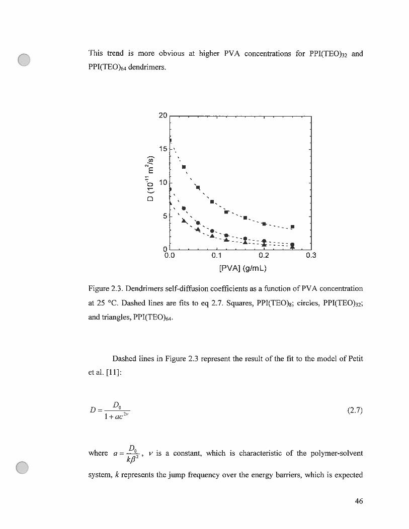
OThis trend is more obvious at higher PVA concentrations for PPI(TEO)32 and

PPI(TEO)64 dendrimers.

20

15U)

I’

t- ts

Qs

s.

0.3

[PVA] (g/mL)

Figure 2.3. Dendrimers self-diffusion coefficients as a function of PVA concentration

at 25 °C. Dashed unes are fits to eq 2.7. Squares, PPI(TEO)8; circles, PPI(TEO)32;

and triangles, PPI(TEO)64.

Dashed unes in Figure 2.3 represent the resuit ofthe fit to the model of Petit

et al. [11]:

DD0

(2.7)1 + ac2v

where a = y is a constant, which is characteristic of the polymer-solvent

system, k represents the jump frequency over the energy barriers, which is expected

46

to depend on temperature and size of the diffusant, and e is the polymer

concentration. Thisjump frequency can be written in an Arrhenius form:

k=fexpC’) (2.8)

where f is a frequency prefactor and AE is the height of the potential barrier. The

model of Petit et al. treats the polymer solution as a transient statistical network,

through which the diffusant diffuses in a series of jumps over a potential barrier

determined by the correlation length. Thus, when decreases, there is an increase in

the energy barrier that the diffusant molecule has to overcome to diffuse in the

polymeric network.

The model was used to fit the variation of the self-diffusion coefficient as a

function of PVA concentration for ail dendrimers (and at different temperatures as

well). The values of the parameters D0, k2 and y obtained from the fit with eq 2.7

are listed in Table 2.3. It shows that excellent agreement of the D0 values obtained

from fitting to the ones measured by the NMR experiments. The margin of errors for

ail the parameters is veiy small, indicating the high quality of the fiftings. The D0

values in the table decrease with the molecular weight. This resuit agrees well with

eq 2.4, which links the self-diffusion coefficient with the inverse of the cubic root of

the molecular weight. When the strength of the interactions between the diffusing

molecules and the polymer matrix is strong enough, this trend could be reversed.

Moreover, we have observed that the kfl2 parameter decreases with increasing

molecular size of the diffusing dendrimers (see figure 2.4). The dashed une serves as

visual guide of the decrease in k/32 and has no physical meaning. Since fi remains

constant for a given polymer-solvent system [11], the resuits obtained conïirm that an

increase in the molecular size leads to a lowerjump frequency [4, 11, 27]. Consistent

with the resuits reported by Masaro et al. for PEGs as diffusant [13], the kfi2

parameter decreases with the molecular size of the diffusant. for example, the kfi2

(J” parameter for PEGs with molecular weights of 600, 2000 and 4000 decreased from

47

1.20 x i0 to 0.47 x 10h1

G

Table 2.3. Self-diffusion coefficients (D0), hydrodynamic radii tRh) and titting

kfl2 and y parameters obtained for the dendrimers in aqueous PVA systems

D0 (10’’m2/s) k/32 a

aRh” RMS’

samples uexp. calc.a (1011) (nm) error

PPI(TEO)g 16.4±0.2 16.4±0.3 0.79±0.09 0.59±0.03 1.21 0.06

PPI(TEO)32 9.1 ± 0.1 9.1 ± 0.1 0.16 ± 0.01 0.6$ ± 0.02 2.18 0.06

PPI(TEO)64 7.0 ± 0.3 6.9 ± 0.2 0.10 ± 0.02 0.69 ± 0.04 2.86 0.06

(a)obtajfled as a fitting parameter from eq 2.7.

(b)calculated from eq 2.5.

errors ofthe nonlinear least-square fiffing to eq 2.7.

1.0 I I

0.8U)

1.52:O25 3.0

Rh (nm)

figure 2.4. Variation of the kp2 parameter as a function of the hydrodynamic radius

ofthe dendrimers at 25 °C. The dashed une is drawn only as visual guide.

4$

To compare two diffusants with similar molecular weights, the kfl2 parameter

obtained for PPI(TEO)8 is 0.79 x 10h1 while that for PEG-2000 is 0.53 x 10h1,

indicating that the jump frequency for the dendrimer is somewhat higher than that of

the linear PEG.

The values ofthe vparameter in Table 2.3 are in the same range ofthe values

(0.49 to 0.76 with an average of ca. 0.5$) reported by Masaro et al. for other

diffusants in the same polymer-solvent system under the same conditions [4, 26, 27].

This y parameter seems to be characteristic of a given polymer-solvent system and is

independent ofthe diffusing molecule.

The model describes well the variation of the self-diffusion coefficient of the

dendrimers in the PVA-water-dendrimer temary system. Theoretically, the model of

Petit et al. should be valid only when e is superior or equal to the critical overlap

concentration (c*), the concentration at which intermolecular entanglements between

polymer chains can occur.As shown in Figure 2.3, the obtained fitting curves with the

model of Petit et al. are continuous for the entire concentration range of PVA,

including the dilute regime.

Table 2.3 reports the effective hydrodynamic radius (Rh) obtained for each

dendrimer from the Stokes-Einstein equation (eq 2.5). The hydrodynamic radii for

our modified dendrimers are somewhat larger than those obtained by Rietveld et al.

[44] for PPI dendrimers with primary amine end groups. The difference should

correspond to the extra length ofthe added TEO groups on the PPI dendrimers.

The density distribution of dendrimers and linear polymers coils depends on

many factors including the quality of the solvent, the temperature, the size of the

dendrimer and the molecular weight of the polymer. b obtain a qualitative

evaluation of the density distribution, D0 and Rh were plotted as a function of the

molecular weight. Figure 2.5A is a logarithmic plot of D0 and Rh as a function of the

molecular weight. The values of the siope obtained for both variations are identical

but have opposite signs (slope = 0.40). This result indicates that the density

distribution is between a fractal structure (slope = 0.50) and a uniform density

distribution (siope 0.33) [44]. Apparently, the siope of 0.40 differs from that

C indicated in eq 2.4 (0.33), but it is important to note that the dendrimers are neither

49

(Dspherical in shape nor uniform in density.

-8.0 -8.0

A-8.5 -8.5

._

-9.0 -9.0

D)o-J

-9.5 -9.5

4

-10.0 . -10.0

-10.5 II -10.5

-8.0 -8.0

B

-8.5 . - - -. -8.5

-I—--.

o -9.0 --9.0

D) D)o o

-9.5 -9.5

-10.0 4 •- -10.0

..-.

-10.5 I -1052.5 3.0 3.5 4.0 4.5

Log M

figure 2.5. Dependence of D0 and Rh of dendrimers (A) and PEG (B) on their

molecular weights at 25 °C.

50

It would be interesting to compare the resuit with that of linear PEGs from the

ilterature [22]. The data in figure 2.5B show the dependence of Do and Rh on the

molecular weight for PEGs (M = 600 10 000). The siope obtained for these linear

polymers is equal to 0.49, which indicates that the linear diffusants such the PEGs

have a fractal density distribution. Understandably. the PEGs as diffusants are less

uniform in density than the dendrimers used in this study.

2.4.3.2. Effect of Temperature

The self-diffusion coefficients of the modified poly(propyleneimine)

dendrimers were determined over a temperature range from 5 to 45 °C for eight

different PVA concentrations. An example ofthe resuits is shown in figure 2.6A for

the variation of the self-diffusion coefficient of PPI(TEO)8 dendrimer with PVA

concentration (from O to 0.26 g/mL). As expected, D increases with increasing

temperature, but the effect of temperature becomes less significant with increasing

PVA concentration. This decrease is due to the intermolecular entanglements and

hydrogen bonding between polymer chains near and above the critical overlap

concentration (c*). In the case of PVA-water system, the c is mostly affected by the

molecuÏar weight and the degree of hydrolysis and its value is between Ï to 5%

(using the definition c = 1/[Ti1) [45-47]. It can also be viewed as the concentration

of the transition from the dilute regime, where the cous are isolated, to a more

concentrated state, where the cous entangle. Above this c, a fundamental change in

the physical properties of the polymer solutions occurs (e.g. the viscosity behavior)

[48-49]. As shown previously [45, 50], no critical effects have been observed by self-

diffusion measurements. The same behavior (i.e., the reduction of the temperature

effect on the self-diffusion coefficient at higher PVA concentrations) was observed

for the two other dendrimers (PPI(TEO)32 and PPI(TEO)64). Moreover, the effect of

the temperature on the self-diffusion coefficient is less significant with increasing

molecular weight of the dendrimers (data not shown). This resuit agrees well with eq

2.4, which links the self-diffusion coefficient with temperature and the inverse ofthe

cube root of the molecular weight. It is obvious from this equation that D should be

less affected by the same temperature variation when the molecular weight is higher.

51

o

30A

• 5°C

• 15°C

- 20 À25°cy 35°C

• 45°CV 5 ‘

À

D n -

..

s * ‘r..À’V

_:L. ::I- E--.•••_---.

--.. -----t

i.0 B

0.8‘À

• 5°C

• 15°C

2’ A 25°C

0.6 ‘y 35°C

Q I •45°C

D ss

0.4 L

0.2 ‘---t0.0

0.0 0.1 0.2 0.3

[PVAJ (g/mL)

Figure 2.6. (A) Self-diffusion coefficients and (B) normalized self-diffusion

coefficients (D/D0) of the PPI(TEO)g dendrimer as a function of PVA concentration

at five different temperatures. Dashed unes are fits to eq 2.7.

52

Another interesting observation is that the dependence of the self-diffusion

coefficients of the dendrimer on temperature may be iargely contained in the self-

diffusion coefficient of the diffusant in the pure soivent (D0). Figure 2.63 shows the

normalized diffusion coefficients (D/Do) for the same PPI(TEO)8 dendrimer as a

function of polymer concentration at various temperatures. The data points foiiow

the same trend and are seen to fali more or less on the same une fitted with eq 2.7.

Similar resuits are obtained with the other dendrimers used in this study.

Dashed unes in F igure 2.6 are the resuit of the fit with the model of Petit et ai.

(eq 2.7). Excellent fitting is obtained for the variation of the self-diffusion coefficient

with PVA concentration for ail temperatures. The self-diffusion coefficient at zero

polymer concentration (D0) was used to show the effect of the temperature on the

density distribution of these tbree dendrimers (Figure 2.7).

-9.3

-9.6 - -

o - S

D S S

-9.9- -

--

-

-10.2

I-

-10.5 I

3.0 3.5 4.0 4.5Log M

Figure 2.7. Dependence of D0 of dendrimers on molecular weight at three different

temperatures. Squares, circies and triangles represent the values obtained at 5, 25

and 45 °C, respectively.

53

C.figure 2.7 shows the variation ofthe logarithm of D0 as a function ofthe logarithm of

molecular weight at three different temperatures (5, 25 and 45 °C). The values of the

siope obtained are —0.39, —0.40 and —0.39 for 5. 25 and 45 °C, respectively. These

resuits show no effect of the temperature on the density distribution of the dendrimers

within this temperature range. From the D0 values determined with the model of Petit

et al., the hydrodynamic radius was calculated with the Stokes-Einstein equation (eq

2.5) at different temperatures. The results in Figure 2.8A show a decrease of Rh with

increasing temperature for these three dendrimers. However, the decrease is more

obvious for dendrimers with higher molecular weight (PPI(TEO)32 and PPI(TEO)64).

This may be due to the effect of the quality of the solvent, which decreases with

increasing temperature [51]. When the solvent quality decreases, the dendrimers

shrink, which leads to a decrease in Rh. This phenomenon affects higher molecular

weights first because they are more sensitive to the solvent quality. This phenomenon

is used in the fractionation of polymers. Stechemesser et al. obtained the same resuit

in their study of the effect of soïvent quality on the self-diffusion coefficient of

tetrafunctional poly(amidoamine) dendrimers by holographic relaxation spectroscopy

[51]. However, this decrease with temperature is small (inferior or equal to 14%).

The result in figure 2.$A indicates that the properties of these dendrimers may be

sensitive to temperature. Figure 2.83 shows the variation of the i’ parameter with

temperature. This solvent quality is slightly affected as shown by the small decrease

in the value of u at a higher temperature, but, in general, the variation of y with

temperature and with the diffusant is small as shown in Figure 2.8B, indicating the

parameter is characteristic of a given polymer-solvent system.

The variation of the self-diffusion coefficients with the temperature can be

used to determine the diffusional activation energy (Ea) with an equation similar to

the Arrhenius equation:

D (T) Dr, exp(— Ea /RT) (2.9)

where D is the self-diffusion coefficient at infinite temperature.

54

o

3.5 . I • I • I • I

A3.0

À À ÀÀ

2.5 À

E •E .2.0

1.5

1.0 .

0.5 I • I

2.0 • • I I

B15

1.0

>

6 60.5 • . *

0.0

-0.50 10 20 30 40 50

T (°C)

Figure 2.8. Variation of the hydrodynamic radius (Rh) (A) and the y parameter in the

model of Petit et al. (B) with the temperature for the three dendrimers. Squares,

PPI(TEO)s; circles, PPI(TEO)32; and triangles, PPI(TEO)64.

55

Figure 2.9 shows the temperature dependence of the PPI(TEO)32 dendrimer as a

function of the inverse of the temperature for four different PVA concentrations. The

Arrhenius equation ailows a good fit to the variation of D, observed for ail regimes

(straight unes in Figure 2.9) and shows the accuracy ofthis approach. Figure 2.9 also

shows a continuous increase of the siope with the polymer concentration, which

implies an increase ofthe diffusional activation energy.

—21

-22

-23.- -

D - -u-24 -

_J -

-Â

-25 ‘ .. - - -

-26

V-

-27 I • t • I • I I

3.1 3.2 3.3 3.4 3.5 3.6 3.7

iooorr (K)

Figure 2.9. Semilogarithmic plot of the self-diffusion coefficients of the PPI(TEO)32

dendrimer as a function of reciprocal temperature for four PVA concentrations.

Squares, 0.00 g/mL; circies, 0.06 g/mL; upward triangles. 0.16 g/mL; and downward

triangles, 0.26 g/mL.

Ibis increase is clearly visible in Figure 2.10, which shows the rapid increase in the

diffusional activation energy with the polymer concentration. We can also see an

increase of this energy with the molecular weight for each PVA concentration. The

dashed une is drawn as visual guides. Ail these resuits indicate that the diffusing

56

molecule requires more energy at higher molecular weight and at higher polymer

concentration to escape its present surrounding and move into an adjacent

environment. As for the determination of diffusional activation energy by the

variation of the self-diffusion coefficient with temperature, the same Arrhenius

approach was used with the kfi2 parameter to obtain the apparent activation energy

(Figure 2.11), since we assume that fi is a constant within the temperature range

studied here. A good linear reiationship is obtained for ail dendrimers. The apparent

activation energies obtained are 28.0, 36.1 and 40.9 kJ/mol for the PPI(TEO)g,

PPI(TEO)32 and PPI(TEO)64 dendrimers, respectively.

34

32

s30

o -

— — a— —

-- -.- -

w -- -- --

26 -

24

22’0.0 0.1 0.2 0.3

[PVAJ (g/mL)

Figure 2.10. Variation of the diffusionai activation energy with the PVA

concentration for three dendrimers: Squares, PPI(TEO)8; circies, PPI(TEO)32; and

triangles, PPI(TEO)64. The dashed line is drawn only as visual guide.

According to the model of Petit et ai. [11], these resuits confirm that the iarger

difftising molecuie has a lower jump frequency and thus needs an higher energy to

escape its present surrounding to diffuse in the polymeric network. In comparison to

57

the resuits obtained by Masaro et al. with PEG diffusants [4], the energy barriers of

the dendrimers can be related to that obtained for ethylene glycol (Rh 0.24 nm) and

two PEG samples with molecular weights of 600 and 2000 (Rh = 1.25 and 2.27 nm,

respectively), which have Ea values of 30.0, 36.5 and 39.0 kJ/mol, respectively.

AÏthough the dendrimers used here generally possess higher molecular weights than

the linear PEGs studied, the energy barriers for the dendrimers are much lower in

comparison with the linear PEGs. for the one that is comparable in molecular weight,

PPI(TEO)8 has a similar molecular weight as PEG-2000. but its energy barrier is

much lower (2$ kJ/mol for PPI(TEO)8 vs 39 kJ/mol for PEG-2000).

-24

-25- E = 28.0 kJ/mol•-

-26. -.

-4. -

C - E =36.1 kJ/mol•-27 -À. •

-28

E = 40.9 kJ/mol

-29 I -

3.1 3.2 3.3 3.4 3.5 3.6 3.7

1000/T (K1)

Figure 2.11. $emilogarithmic plot of the k/32 parameter as a ftmction of reciprocal

temperature for the three dendrimers. Squares, PPI(TEO)g; circles, PPI(TEO)32; and

triangles, PPI(TEO)64.

it is possible that ethylene glycol and PEG can form hydrogen bonds more easily

with the polymer matrix and with the aqueous sunounding in comparison to the

5$

dendrimers. For each dendrimer, the activation energy value obtained with the model

of Petit et al. (Figure 2.11) is higher than the diffusional activation energy (Figure

2.10). The difference is flot yet well understood. However, it seems that the apparent

activation energy obtained from kfl2 can be reiated to the maximum energy that the

diffusing molecule has to overcome to diffuse in the polymer matrix at gel polymer

concentration.

2.5. Conclusion

It is clearly shown that the self-diffusion coefficients of the dendrimers

decrease with increasing molecular size of the diffusant, with increasing PVA

concentration, but with a decreasing temperature. The physical model of Petit et aï.

has been used successftully to describe the variation of the self-diffusion coefficient

with the molecular size of the dendrimer, the polymer concentration and the

temperature. These results show that the larger diffusing molecule needs higher

activation energy to escape its present surrounding and to move into an adjacent

environment. It is also the case when the polymer concentration increases. The

apparent activation energy of diffusion varies in the range 28.0-40.9 kJ/mol from

PPI(TEO)8 to PPI(TEO)64 dendrimers. The study shows that the dendrimers have a

density distribution between a fractal structure and a uniform density distribution and

that the temperature in the range 5-45 oc has no effect on the density distribution. In

comparison to the fractal structure obtained for linear PEGs, dendrimers have a more

uniform density distribution. The $tokes-Einstein hard sphere radii have also been

calculated at the zero concentration limit and we have observed an increase of Rh

with the dendrimer generation. However, the results show a slow decrease in Rh with

the temperature for these three dendrimers. The study of the motion of different parts

of the dendrimers by NMR relaxation time measurements shows that the terminal

protons are more mobile than the core protons for ail dendrimers. The relaxation time

measurements also show a decrease in the mobility for ah protons along with

increasing dendrimer generation.

2.6. Acknowledgments

The financial support from the Natural Sciences and Engineering Research

59

Council (NSERC) of Canada and the National Science foundation (USA) is

gratefully acknowledged.

2.7. References and notes

[1] Hariharam, D.; Peppas, N. A. I Controlled Release 1993, 23, 123-136.

[2] Clericuzio, M.; Parker, W. O.; Soprani, M.; Mdrei, M. Solid State Jonics

1995, 82, 179-192.

[3] Gao, P.; Fagerness, P. E. Fharm. Res. 1995, 12, 955-964.

[4] Masaro, L.; Zhu, X. X.; Macdonald, P. M. Macromolecules 1998, 31, 3880-

3885.

[5] Fujita, H. Adv. Polym. Sel. 1961, 3, 1-47.

[6] Yasuda, H.; Lamaze, C. E.; &enberry, L. D. MakromoÏ. Chem. 1968, 118, 19-

35.

[7] Vrentas, J. S.; Duda, J. L. I Polym. ScL, PoÏyrn. Phys. Ed 1977, 15, 403-4 16.

[8] Vrentas, J. S.; Duda, J. L. I Polym. $ci., Polym. Phys. Ed 1977, 15, 4 17-439.

[9] Philties, G. D. J. Macromolecules 1986, 19, 2367-2376.

[10] Vrentas, J. S.; Vrentas, C. M. Macromolecules 1994, 27, 4684-4690.


29, 603 1-6036.

[121 Amsden, B. Macromolecules 1998, 3], $382-$395.

[13] Masaro, L.; Zhu, X. X. Prog. Polym. Sel. 1999, 24, 73 1-775.

[14] Nesmelova, I. V.; Skirda, V. D.; Fedotov, V. D. Biopolymers 2002, 63, 132-

140.

[15] Seland, J. G.; Ottaviani, M.; Hafskjold, Bjøml Colloidlnterf Sel. 2001, 239,

16$-177.

[16] Derrick, T. S.; Larive, C. K. Appi. $pectrosc. 1999, 53, 1595-1600.

[17] Penke, B.; Kinsey, S.; Gibbs, S. J.; Moerland, T. S.; Locke, B. R. I Magn.

60

Reson. 1998, 132, 240-254.

[1$] Manz. B.; Callaghan, P. T. Macromotecutes 1997, 30, 3309-3316.

[19] Yokoyama. H.; Kramer, E. J.; fredrickson, G. H. Macromolecules 2000, 33,

2249-2257.

[201 Nydén, M.; S&lerman, O. MacromolecuÏes 1998, 31, 4990-5002.

[21] Waggoner, R. A.; Blum, F. D.; MacEiroy, J.M.D. Macromolecules 1993, 26,

6841-6848.

[22] Baille, W. E.; Malveau, C.; Zhu, X. X.; Marchessault, R.H.

Biomacromolecules 2002, 3, 214-218.

[23] Malveau, C.; Beaume, F.; Germain, Y.; Canet, D. I PoÏym. 3d. Part B:

Polym. Phys. 2001, 39, 278 1-2792.

[24] Rouet, A.-L.; Simonin, J.-P.; Turq, P.; Gebel, G.; Kahn, R.; Vandais, A.;

No1, J.-P.; Malveau, C.; Canet, D. I Phys. Chem. B 2001, 105, 4503-4509.

[25] Petit. J.-M.; Zhu, X. X.; Macdonald, P. M. Macromolecules 1996, 29, 70-76.

[26] Masaro, L.; Ousalem, M.; Baille, W. E.; Lessard, D.; Zhu, X. X.

MacromolecuÏes 1999, 32, 4375-4322.

[27] Masaro, L; Zhu, X. X.; Macdonald, P.M. I PoÏym. 3d. . Part B : Polym.

Phys. 1999, 37, 2396-2403.

[28] Masaro, L.; Zhu, X. X. MacromoÏecules 1999, 32, 53 83-5390.

[29] Yonetake, K.; Masuko, T.; Morishita, T.; Suzuki, K.; Ueda, M.; Nagahata, R.


[30] Uppuluri, S.; Keïnath, S. E.; Tomalia, D. A.; Dvomic P. R. Macromolecules

1998. 31, 4498-45 10.

[31] Scherrenberg, R.; Coussens, B.; van Viiet, P.; Edouard, G.; Brackman, J.; de

Brabander, E. Macromolecules 1998, 31, 456-461.

[32] Roover, J.; Zhou, L.-L.; Toporowski, P. M.; van der Zwan, M.; latrou, H.;

O Hadjichristidis, N. Macromolecules 1993, 26, 4324-4331.

61

[33] Pan, Y.; Ford, W. T. Macromolecules 1999, 32, 5468-5470.

[34] Chai, M.; Niu, Y.; Youngs, W. J.; Rinaldi, P. L. J Am. Chem. Soc. 2001, 123,

4670-4678.

[35] Pan, Y.; ford, W. T. Macromolecules 2000, 33, 373 1-3738.

[36] Kreider, J. L.; Ford, W. T. I Polym. Sci. Part A: PoÏym. Chem. 2001, 39,

821-832.

[37] Tanner, J. E. I Chem. Phys. 1970, 52, 2523-2526.

[3$] Callaghan, P. T.; Trotter, C. M.; Jolley, K. W. I Magn. Reson. 1980, 37, 247-

259.

[39] Stilbs, P. Prog. Nuci. Magn. Reson. Spectrosc. 1987, 19, 1-45.

[40] Price, W. S. Concepts Magn. Reson. 1997, 9, 299-336.

[41] Amman, C.; Meier, P.; Merbach, A. E. I Magn. Reson. 1982, 46, 3 19-322.

[42] Waldeck, A. R.; Kuchel, P. W.; Lennon, A. J.; Chapman, B. E. Prog. NucÏ.

Magn. Reson. Spectrosc. 1997, 30, 39-68.

[43] De Gennes, P. G. Scaling Concepts in Polymer Physics; Comeil University


[44] Rietveld, I. B.; Bedeaux, D. MacromolecuÏes 2000, 33, 79 12-7917.

[45] Cosgrove, T.; Griffiths, P. C. Polymer 1994, 35, 509-513.

[46] Fang, L.; Brown, W. MacromolecuÏes 1990, 23, 3284-3290.

[47] Te Nijenhuis, K. Adv. Polym. $ci. 1997, 130, 36-52.

[4$] Ferry, J. D. Viscoelastic Properties ofPolymers, Wiley: New York, 1980.

[49] Flory, P. J. Principles ofPolymer Chemistry, Corneil University Press: Ithaca,

NY, 1953.

[501 Skirda, V. D.; Sundukov, V. I.; Maklakov, A. I.; Zgadzai, O. E.; Gaturov, R.

R.; Vasiljiev, G. I. Polymer 1988, 29, 1294-1300.

[51] $techemesser, S.; Eimer, W. Macromolecules 1997, 30, 2204-2206.

62

G

Chapitre 3

Study of Self-Diffusion of Hyperbranched

Polyglycidols in Poly(vinyl alcohol) Solutions

and Gels by Pulsed Field Gradient NMR

Spectroscopy

W. E. Baille, X. X. Zhu, S. Fomine MacromolecuÏes 2004, 37, $569-$576

o

3.1. Abstract

In an effort to further understand the effects of molecular size and shape of

macromolecular diffusants on the diffusion in hydrophilic polyrner solutions and

gels, hyperbranched polyglycidols have been synthesized as hydrophilic diffusants

and characterized. Four of these hyperbranched polymers were selected for the study

of self-diffusion by pulsed-field gradient NMR spectroscopy in poly(vinyl alcohol)

water systems. The effects of the molecular weight, size and shape of the diffusant,

polymer concentration, and temperature have been studied. For diffusants of similar

molecular weight and without specific interactions, the activation energy decreases

from the dendrimers to hyperbranched polymers and then to linear polymers. The

resuits indicate that the molecular shape, hence the molecular density distribution of

the diffusants, is important in the diffusion process.

o64

3.2. Introduction

The molecular diffusion in polymer matrices lias been studied by different

techniques. Examples include cooperative diffusion of giobular protein in solution by

dynamic light scattering [1], probe diffusion by Taylor dispersion and

phosphorescence quenching [2], drug release from polymer gels by gravimetric

measurements [3], and solute diffusion in hydrogels by pulsed fieÏd gradient (PFG)

NMR techniques [4]. The results of these studies helped in the understanding of the

diffusion phenomena in polymer systems. The effects of polymer concentration, size

and shape of the diffusant, temperature and specific interactions within the polymer

matrix are ail important in determining the diffusion properties in a polymer system,

which ultimately determines the applicability of polymeric materials in industry.

Also, the data allowed to develop and to test over the years various physical modeis

of diffusion [5-13]. The physicai models of diffusion are essential for the

interpretation of the resuits.

The molecular size and shape of the diffusants are known to have an effect on

the diffusion of plasticizers in poly(vinyl chloride) [14-16] and in epoxy resins during

curing [17], and in poly(methyl methacryiate) [18, 19]. We have studied the self-

diffusion of solute molecules ranging from small molecules to polymers and from

linear to more spherical molecules in polymer solutions and gels [11, 20-241 in an

effort to elucidate the effects of functional groups (alcohol, amine, ammonium sait,

amide and acid) [11, 20], diffusant size and shape, poiymer concentration, and

temperature in the diffusion process [21-24]. Recently, our study showed the

difference in the activation energy between poiy(propylene-imine) (PPI) dendrimers

with hydrophilic triethylenoxy methyl ether (TEO) terminai groups and linear

poly(ethylene glycol)s (PEGs) of comparable molecular weights [24]. The resuits

show that the self-diffusion coefficient is greater for the dendrimers than the linear

PEGs when the molecular weights and experimental conditions are similar. The same

trend was observed for various polymer concentrations.

b obtain a better understanding of the shape effect on the self-diffusion of

the molecuies and to put the mode! of Petit et al. on a more rigorous footing, we have

(J made four hyperbranched poiygycido!s and studied their self-diffusion in po!y(viny!

65

alcohol) (PVA) solutions and gels by PFG NMR spectroscopy. These molecules can

be considered to possess intermediate shapes between linear polymers and more

spherical dendrimers. Therefore, a comparison is also made with previous data

obtained with linear PEGs and dendrimers.


3.3.1. Materia]s

Glycidol (96%), dioxane, potassium methoxide (95%) and ail other chemicals

were purchased from Aldrich (Milwaukee, WI). D20 was purchased from C.I.L.

(Andover, MA). Ail chemicals were used as received.

3.3.2. Preparation of Hyperbranched Polyglycidol (HBPG) [25, 26]

Glycidol (50 g, 675 mmol) was added dropwise under a nitrogen flow during

12 hours at 90 °C into a suspension of potassium methoxide (0.25 g, 3.5 mmol) in

dioxane (50 mL). When the reaction was completed, dioxane was removed under

vacuum and polyglycidol was obtained as very viscous syrup. The polymer was

neutralized with concentrated HC1.

HBPG was fractionated on a preparative size exclusion chromatography

system equipped with two columns ($hodex OHpak SB-2003 and 2004). The ftow

rate of the eluent was at 2.0 mL/min. The columns and the detector were equilibrated

at 33 and 35 °c, respectively.

3.3.3. Size exclusion Chromatography (SEC)

The molecuiar weight of seiected polymer fractions was measured on a $EE

system equipped with a Waters 1525 binary HPLC pump, a Waters 2410 refractive

index detector and a set ofthree Ultrahydrogel colunms (Ultrahydrogel 120, 500 and

2000). Poly(ethylene glycol) (PEG) and poly(ethylene oxide) (PEO) were used as

standards for the calibration. The polymers were dissolved in water at a concentration

of 2 mg/mL and fiitered through 0.45 jim filters before injection. The flow rate ofthe

eluent was at 0.5 mL/min. The columns and the detector were equiiibrated at 33 and

35 °C, respectively.

3.3.4. NMR Spectroscopy

1H NMR, inverse gated 13C NMR and DEPT-135 (distortionless enhancement

by polarization transfer) experiments of the polymer samples in DMSO-d6 and D20

66

(with a small amount of copper sulfate as relaxation agent) were performed on a

Bruker AV-400 spectrometer operating at a frequency of 400.13 MHz for ‘H and

100.63 MHz for 13C to characterize the hyperbranched polyglycidols.

3.3.5. MALDI-TOF Mass Spectrometry

The molecular weight of ail samples was aiso measured by using Kratos

Kompact MALDI-Ili TOF mass spectrometer benchtop model. The system generates

a maximum laser output of 6 mW at a waveiength of 337 nm (N2 laser light, 3 ns

pulse width). All the samples in this study were analyzed by using the reflection

mode to obtain a higher mass resolution. Œ-Cyanohydroxycinnamic acid was used as

the matrix. Before the molecular weight measurement, samples were prepared by

dissolving the hyperbranched polymers in water at a concentration of 5 mg/mL. Into

this solution, 10 mg/mL of the matrix aqueous solution and 5 mg/mL of LiBr

aqueous solution were added. 0.1 iL of this mixture was applied to a spot on a

sample slide and the solvent was allowed to evaporate slowly to create a thin matrix

analyte film [27].

3.3.6. Pulsed Fieid Gradient NMR Measurements

To measure the self-diffusion coefficient (D), samples were prepared

following the method described previously [11, 21]. PVA (M = 52 000 with a degree

of hydrolysis equal to 99%) was added to a D20 solution containing 1 wt % of

diffusant in 5 mm o.d. NMR tubes. The concentration of PVA ranged from O to 0.32

g/mL.

D values were determined using the stimulated echo (STE: 90°-t1-90°-t2-90°-

ti-echo) technique developed by Tanner [2$] on a Bruker DSX-300 NMR

spectrometer operating at a frequency of 300.1$ MHz for protons. Details on the

NMR experiments were described previously [24]. The self-diffusion coefficients

were extracted by using the following expression [29-311

in-L = __L_ln2 —y22G2D(A —5/3) (3.1)I 77

67

where I and b are the NMR signal intensities in the presence and in the absence of

the gradient and the relaxation processes, respectively, ti is the intervai between the

first two 900 r.f. pulses and between the third 90° r.f. pulse and the middie of the

echo, t2 the delay between the second and the third 90° r.f. pulses, ythe gyromagnetic

ratio of the nucleus under observation, T1 and T2 the spin-lattice and the spin-spin

relaxation times, respectively, 5 and G the duration and the strength of the applied

gradient puise, respectiveiy, D the self-diffusion coefficient, and A the time intervai

between the two successive gradient pulses (also called the diffusion time). The self-

diffusion coefficient was extracted from the siopes of the unes obtained from linear

regression of the logarithm of signal intensity as a function of G2. Excellent linear

relationships have been obtained in these experiments with correlation coefficients of

0.985 and better. The error of the measured D values was estimated to be 7% by

carrying out repeated experiments with seiected sampies. The accuracy of results can

be detennined by studying samples with lmown self-diffusion coefficients such as

pure water and pure glycerol, and good agreement was obtained at 25 oc with values

reported in the literature [32, 33].

The experiments were performed at different temperatures for ail HBPG

samples at 25, 35, 45 and 55 oc (fluctuation of the temperature ± 0.3 oc) and

concentrations of PVA ranged from O to 0.32 g/mL. Temperature calibration was

done periodicaiiy on the NMR instrument by measuring the chemical shifi difference

between the ‘H NMR signals of CH2 and OH groups of pure ethylene glycol at

various temperatures since this difference is sensitive to temperature changes [34].

A noniinear least-square fitting method was used in ail cases to fit the

experimental diffusion data to the model of Petit et al. [11] The correlation

coefficients r2 yielded were in the range of 0.989 0.999. The quality of the fitting to

the experimental data was also indicated by the good fits shown in ail the figures.

The same sets of fitting parameters were obtained regardless of the initial values used

in the procedure.

3.4. Results and Discussion

C 3.4.1. Characterization of Hyperbranched Polyglycidols

68

from glycidol monomers, HBPGs have been synthesized by ring-opening

polymerization initiated with potassium methoxide. During the initiation a primary

aikoxide and a secondary aikoxide can be formed. In the propagation step, these two

aikoxide species can both react with glycidol. The structure of resulting polymers is

shown in figure 3.1. Both intermolecular and intramolecular chain transfers can take

place [26]. Macrocyclic products may also be formed [26] if the primary aikoxide

reacts with the epoxy group from glycidol monomer.When the reaction is completed,

a light yellow viscous liquid is obtained.

The number-average molecular weight (Ma) of the product determined by

SEC was ca. 3000 g/mol with a polydispersity of 2.9. The HBPG was then fractioned

by preparative SEC. The molecular weight and the polydispersity obtained by SEC

for four selected fractions are listed in Table 3.1. However, these molecular weights

are only relative to the linear PEG and PEO used as standards. To obtain a basis of

comparison ofthe molecular weights, MALDI-TOF mass spectrometry was also used

for the characterization.

Figure 3.1. Schematic structure of the hyperbranched polyglycidol. Examples of the

dendritic segment (De), linear 1,3- segment (Li3), linear 1,4-segment (L14) and

terminal segment (T) as indicated by concentric unes.

HO

HI

69

QTable 3.1. Determination of the Molecular Weights of HBPGs by SEC and

MALDI-TOF Mass Spectrometry

SEC MALDI-TOFS amples

Ma M/Mb IVIa Iv1v/Mnb

HBPG-i 226 1.14 324 1.81

HBPG-2 672 1.48 629 1.18

HBPG-3 1 $90 1.26 1102 1.44

HBPG-4 3245 1.19 1868 1.02

(a)Number.average molecular weight

(b)Pldiity

The number-average molecular weights obtained for samples HBPG-1 and HBPG-2

by the MALDI-TOF technique are in good agreement with the SEC resuits (Table

3.1). For HBPG-3 and HBPG-4, the degrees of branching (DB) (See Table 3.2 and

the discussion below) are higher and the differences of M obtained with the two

analytical methods are larger. The deviation of the SEC resuits for HBPG-3 and

HBPG-4 may resuit from the use of linear PEGs as standards in the measurements of

hyperbranched polymers. The M and the polydispersity obtained by MALDI-TOF

are used in the analysis of the resuits in this study since we consider that these values

are not affected by the choice of calibration standards as in SEC. Even so, the ion

formation in the MALDI-TOF method may resuit in the breaking up of the

polyglycidol chains which may yield lower M than the real values, especially when

the reflectron mode is used [35].

Quantitative inverse gated ‘3C NMR spectra and DEPT- 135 spectra of the

polymers are used to identify the structure of each HBPG fraction. Figure 3.2 shows

the ‘3C NMR and DEPT-135 spectra obtained for sample HBPG-1. Ail signais have

been assigned by Tokar et al. [36] and Sunder et al. [26], D corresponds to the

dendritic segment, L symbolizes the linear segment and T represents the terminal

70

G

C

segment of HBPG. The linear segment may be composed of either a linear 1,3-unit

(L13) or a linear 1,4-unit (Li4). A L13 segment is obtained when the secondary

hydroxyl group has propagated. L14 segment is obtained when the primary hydroxyl

has propagated.

2L14

2D, 2T.

Figure 3.2. 13C NMR spectrum (A) and DEPT-135 NMR spectrum (B) obtained for

HBPG-1 in DMSO-d6. D corresponds to the dendritic segment ofthe HBPG and L13

and Lsi4 symbolize respectively the linear 1,3-segment and the linear 1,4-segment. T

represents the terminal segment of HBPGs.

Table 3.2 shows the relative abundance in percentage determined from the relative

integrals of the inverse gated 3C NMR signais for each segment of the HBPG.

Apparently, the relative abundance of the segment L13 increases with the molecular

weight. However, segment L14 does flot depend on the molecular weight.

A

T

Ls13

B

Ls13

85 80 75f ppm)

65

71

Nevertheless, the D5 part increases with the molecular weight while the T part

decreases.

Table 3.2. Relative Abundance of Substructure Units and Degree of Branching

(DB) of HBPGs obtained by Inverse Gated ‘3C NMR spectroscopy

Relative Abundance (%)DB

Samples Dendritic Linear 1 ,3 Linear 1,4 Terminal(D) (L513) (Es14) (T)

HBPG-1 7 4 34 55 0.22

HBPG-2 12 14 38 36 0.32

HBPG-3 16 14 35 35 0.40

HBPG-4 19 17 34 30 0.43

Table 3.2 also shows that the relative abundance of segment L514 is aiways at least

twice higher than segment L513, since the primary aikoxide has a lower sterical

hindrance and a higher stability than the secondary aikoxide [26, 37]. This

combination makes primary aikoxide more reactive than secondary aikoxide. From

the relative abundance values in Table 3.2, the DB has been estimated for each

fraction by the general definition of DB for an AB2 system [26, 38, 39]:

DB2D5

(3.2)2D + L13 + L14

The degree of branching measures the suitability of a hyperbranching reaction to

create dendritic structure. Thus, for a linear polymer, the DB is 0. For a

homopolymerization of AB2 monomers, the DB is 0.5 when the two B groups have

the same reactivity during a random potymerization. In the case of a perfect dendritic

72

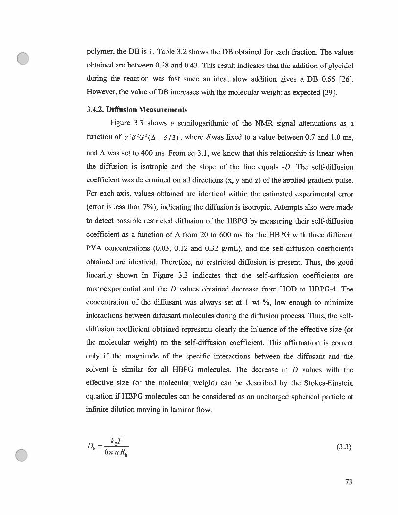
polymer, the DB is 1. Table 3.2 shows the DB obtained for each fraction. The values

obtained are between 0.2$ and 0.43. This resuit indicates that the addition of glycidol

during the reaction was fast since an ideal slow addition gives a DB 0.66 [26].

However, the value of DB increases with the molecular weight as expected [39].


figure 3.3 shows a semilogarithmic of the NMR signal attenuations as a

function of y262G2( — 6/3), where ôwas fixed to a value between 0.7 and 1.0 ms,

and A was set to 400 ms. from eq 3.1, we know that this reiationship is linear when

the diffusion is isotropic and the siope of the une equals -D. The self-diffusion

coefficient was determined on ail directions (x, y and z) of the applied gradient pulse.

for each axis, values obtained are identical within the estimated experimentai error

(error is less than 7%), indicating the diffusion is isotropic. Attempts also were made

to detect possible restricted diffusion of the HBPG by measuring their self-diffusion

coefficient as a function of A from 20 to 600 ms for the HBPG with three different

PVA concentrations (0.03, 0.12 and 0.32 g/mL), and the self-diffusion coefficients

obtained are identical. Therefore, no restricted diffusion is present. Thus, the good

linearity shown in figure 3.3 indicates that the self-diffusion coefficients are

monoexponential and the D values obtained decrease from HOD to HBPG-4. The

concentration of the diffusant was always set at 1 wt %, low enough to minimize

interactions between diffusant molecules during the diffusion process. Thus, the self-

diffusion coefficient obtained represents clearly the inluence of the effective size (or

the molecular weight) on the self-diffusion coefficient. This affirmation is correct

only if the magnitude of the specific interactions between the diffusant and the

solvent is similar for ail HBPG molecuies. The decrease in D values with the

effective size (or the molecular weight) can be described by the Stokes-Einstein

equation if HBPG molecuies can be considered as an uncharged spherical particle at

infinite dilution moving in laminar flow:

D0 = k8T(3.3)

617Rh

73

Where D0 is the self-diffusion coefficient at zero polymer concentration, k3 the

Boltzmann’s constant, T the absolute temperature, 77 the viscosity of the solvent

(D20) and Rh the effective hydrodynamic radius of the diffusing molecule, which is

related to 17 (the partial specific volume) and M (the molecular weight) of the

diffusant by the following equation [40]:

Rh 31 (34)

4n N

The combination of eqs 3.3 and 3.4 shows clearly that when the shape of the

diffusant is spherical and without any specific interactions between the diffusant and

the solvent, the self-diffusion coefficient must be inversely proportional to the cubic

root of the diffusant molecular weight. To verify qualitatively the shape of HBPG

molecules, the self-diffusion coefficient in the absence of any polymer (Do) and the

effective size (Rh) deduced from eq. 3.3 (Table 3.3) were plotted as a function of the

molecular weight. Figure 3.4 shows logarithmic plots of D0 and Rh versus the

molecular weight. The values of the slope obtained for both variations are identical

but have opposite signs (siope = 0.62). The resulting siope value for HBPG

molecules shows clearly that these molecules are flot spherical in shape, since a slope

value of 0.33 is expected fora spherical diffusant as illustrate by eq 3.4.

Qualitative evaluation of the density distribution (or the fractal dimension) of

polymers can be also deduced from figure 3.4. The slope value obtained corresponds

to the Flory exponent (a), which provides qualitative information on the polymer

conformation in dilutes solutions [24, 41-441. The value obtained for HBPG

diffusants indicates that the density distribution of HBPGs is similar to that of a

swollen polymer chain or polymer in a good solvent [44-48]. Thus, the fractal

dimension value (lia) is equal to 1.62, which indicates that the HBPGs conformation

is like an expanded coil. According to Stancik et al. [46] and King [49], randomly

branched polymers are characterized by l/a = 2 in a good solvent or lia 2.2$ in a

0-solvent. The lia value of HBPG may be a further indication of their relatively

74

lower degree ofbranching as shown in Table 3.2 [50]. In comparison to the previous

resuits obtained for PPI(TEO) dendrimers (siope = 0.40 and lia 2.5) and linear

PEGs (siope = 0.49 and lia 2.0), it is clear that the density distributions for the

three kinds of diffusants are different. In the case of linear PEG, lia corresponds to

polymer cous in a 9-solvent [4$]. For the PPI(TEO) dendrimers, the fractal

dimension value is smaller than the expected value (siope = 0.33 and lia = 3 for a

diffusant with a perfect sphericai shape), indicating a compact space-fihling structure

[441.

• Â V

I •À ‘ *I. W

Ïy

• À

• ‘À

j —2 •s -

3•À

-40.0 4.0x109 80x109 1.2x101°

(Gy)2(A-/3) (slcm2)

Figure 3.3. $emilogarithmic plot of the attenuation of the HBPG NMR signais in a 1

wt % aqueous solution (without PVA) at 25 °C as a function of (Gyô)2 (A—6 i 3),

where 6 is fixed to a value between 0.7 and 1.0 ms and A = 400 ms. Squares, HOD;

circles, HBPG-l; up triangles, HBPG-2; down triangles, HBPG-3 and diamonds,

HBPG-4.

o75

G -20

.-

.--

-21

Û D)D) .2o

-22

_________

I

I-

-23 II • I

6.0 6.5 7.0 7.5

Iog M

Figure 3.4. Dependence of Do and Rh of HBPGs on their molecular weights at 25

oc.

3.4.2.1. Effect of Polymer Concentratïon

Figure 3.5A shows a plot of self-diffusion coefficients of HBPG as a function

ofPVA concentration. As obtained in previous studies in PVA [11, 21, 23, 24], the D

values decrease with the PVA concentration, from O to 0.32 g/mL. This concentration

range covers the dilute to the viscous gel regimes. We assume that at the dilute

regime the decrease of the self-diffusion coefficient is principally influenced by the

viscosity of the PVA solutions. However, the decrease in the D between the semi

dilute and the viscous gel regimes is greatly influenced by the capability of the

polymer chain to form a network at the concentration. By analogy to de Genne’s

scaling laws, this network can be characterized by a correlation length, [51].

According to theses scaling laws [51] and from the description of solute diffusion in

hydrophilic networks by Peppas et al. [52], should decrease rapidly while the

polymer concentration increases. This decrease of with the polymer concentration

76

is a resuit of contacts and entanglements of the polymers. Thus, the increased

contacts and entangiements induce greater difficulties for the diffusant to pass

through the polymer matrix. However, in the viscous gel regime, the decreases

more siowly. Thus, the effect of the poiymer concentration on the self-diffusion

coefficient tends to be iess significant, as iilustrated in figure 3.5A.

figure 3 .5A also shows a dependence of the self-diffusion coefficients on the

molecular weight or the effective size of the diffusant. However, this moiecular

weight effect becomes iess significant for HBPG with higher moiecular weights. The

same resuits have been obtained previously for linear poly(ethyiene glycol) and

hydrophilic dendrimer diffusants [11, 21, 23, 241. Dashed unes in figure 3.5A

represent the result of the fit to the model of Petit et al. as shown in the foilowing

equation [11]

D=D0

(3.5)1+ ac

where a = k represents the jump frequency over the energy barriers, which is

expected to depend on the size of the diffusant and on the specific interactions

bePveen the diffusant and the polymer matrix. The k parameter depends aiso on the

temperature. This jump frequency can be written in an Arrhenius form:

k=FexpÇ) (3.6)

where F is a ftequency prefactor and AE is the height of the potentiai barrier.

The model was used to fit the variation of the self-diffusion coefficient as a

function of PVA concentration for ail HBPGs. If we allow ail parameters (D0, kfl2

and y) to vary, y ranges from 0.4$ to 0.5$ for HBPGs. for ail the fits obtained, the

average value of u in ffiis work and in previous studies was used [21, 22]. This

77

Oaverage value (y = 0.5 8) is approximately equal to the value expected for the case of

a marginal solvent (u = 0.50) [53].

5 I

A

41

E.

c. :Q

‘“s •1 - —.. __--__._

0.8- ‘

0.6- -

DV’D

0.4-

—

—

0.2 -

0.00.0 0.1 0.2 0.3 0.4

[PVA] (g/mL)

Figure 3.5. (A) HBPG self-diffusion coefficients as a function of PVA concentration

at 25 °C. (B) Normalized self-diffusion coefficients (D/D0) ofthe HBPG diffusants as

a function of PVA concentration. Dashed lines are fits to eq 3.5. Squares, HBPG-1;

circles, HBPG-2; up triangles, HBPG-3 and down triangles, HBPG-4.

78

$chaefer and Han have shown that in the semi-dilute regime the exponent y

value obtained from the proportionality equation between the polymer cooperative

diffusion constant (De) and the monomer volume fraction (p) is 0.75 for a good

solvent, 0.5 for a marginal solvent and 1.0 for poor solvent [53]. The values of this

exponent as an indication of the quality of the solvent are essentially the same as

those ofthe Mark-Houwink parameter Œ in the relation Rg = K Mw’. Different resuits

for PVA-water systems have been found in the literature. For example, Horkay et al.

obtained an exponent value 0.77 by dynamic light scattering for PVA concentrations

higher than 0.10 g/mL [54], corresponding to a good solvent. However, flory’s

interaction parameter obtained by the sanie authors ( = 0.424) is close to the

expected value for a 0-system (y = 0.5) [54]. Nevertheless, this value (x 0.484)

indicates that water is a marginal solvent for the range of PVA concentrations used

by Horkay et al [54]. On the other hand, resuits obtained by Wang et al. yielded a

value of 0.56 for the exponent Œ for the PVA-water solutions while a recalculation of

the data provides a value of 0.71. These values correspond to the values expected for

random cous in a 0-solvent (Œ = 0.5) and for polymers in a good solvent (a = 0.75),

respectively [55, 56].

According to de Gennes, a transition from good solvent to poor solvent occurs

at I = 1- 2, where ci is the fraction of sites occupied by monomers if the polymer

solution is taking as a periodic lattice and represents the interaction parameter of

Flory [51]. Using this relation, the transition from good to poor solvent should occur

at a PVA concentration of 0.012 g/mL with = 0.484 [54-57]. This indicates that the

concentration range of PVA used in this study should correspond to the situation of a

poor solvent. However, the PVA-D20 samples were homogeneous as indicated by

the clear solutions so that the solvent should flot be a poor one though it can be a

marginal one (as indicated by the measured y values). The thermal history of a PVA

solution can be important [5$], since the clear PVA solution may become opaque

over time and becomes clear again when heated. The values of the parameters D0 and

k/32 obtained from the fit with eq 5 are listed in Table 3. It shows that excellent

agreement of the D0 values obtained from fitting to the ones measured by the NMR

79

experiments. This comparison is a good indication of the data quality and the

difference is well within the margin of errors obtained (iess than 15% for the

parameters obtained from the fit with the model of Petit et al.). The Do values in the

table decrease with the molecular weight. This resuit agrees weil with eq 3, which

relates the self-diffusion coefficient to the inverse of the cubic foot of the molecular

weight. The kfi2 pararneter observed for ail samples in the Table 3 decreases when

the molecular weight (or size) of HBPG increases. The same decrease has been

observed in previous works [11, 2 1-24]. Since fi remains constant for a given

polymer-solvent system [11], the resuits shown in Table 3 confirm that an increase in

the molecular size leads to a iower jump frequency. Thus, the higher the molecular

weight of the diffusant is the more difficuit it would be for the diffusant to diffuse in

the polymer matrix.

Table 3.3. Experimental Self-diffusion Coefficients (Do), Hydrodynamic Radii

tRh) and Fitfing Parameters kfi2 and D0 Obtained for the HBPG in Aqueous

PVA Systems

Samples Rh(a) D0 (1 0 ‘ °m2/s) kfi2 (b)

R2 (c)

(nm) Exp. Calc.t (10’°)

HBPG-1 0.4$ 4.12 ± 0.01 4.10 ± 0.05 0.29 ± 0.02 0.999

HBPG-2 0.62 3.19 ± 0.01 3.17 ± 0.04 0.18 ± 0.01 0.998

HBPG-3 1.04 1.92±0.01 1.87±0.05 0.10±0.01 0.991

HBPG-4 1.37 1.46 ± 0.01 1.43 ± 0.04 0.07 ± 0.01 0.993

(a)calculated from eq 3.3.

(b)obtained as a fitting parameter from eq 3.5 when the average value of vis used

(0.58).

(c)rootmeansquare errors ofthe non-linear least square fitting to eq 3.5.

Q$0

figure 3.5A shows the effects of molecular weights of the diffusants and of

PVA concentration on the self-diffusion coefficient of HBPGs. However, to obtain

insight into the effect of specific chemical interactions between HBPG and PVA

matrix, we choose to normalize the self-diffusion coefficients (D/Do) and plot them

as a function of PVA concentration. Figure 3.5B shows this normalized diffusion

coefficients (D/D0) of HBPG with different molecular weights as a function of PVA

concentration. The first look of Figure 3.5B shows that the data points of ail

diffusants follow the same trend. Indeed the beginning ofthe curves starts at the same

point and the ends of the curves also seem to converge to similar values. A doser

examination of the curves reveals that in the middle section, the D/D0 values of the

different diffusants vary significantly. This indicates that the effect of interactions

with the polymer network have an effect in the intermediate concentration range of

PVA. Within this concentration range a screening effect becomes possible.

To study the effect of the shape of the diffusants on the self-diffusion

coefficient, comparison can be made among HBPGs, PPI(TEO) dendrimers and

linear poly(ethylene glycol)s with similar molecular weights around 2000 g/mol. The

variation of the self-diffusion coefficient with the diffusant shape is shown in Figure

3.6 and the self-diffusion coefficients ofthe dendrimer are systematically higher than

those of the HBPG. At higher PVA concentrations, the two kinds of diffusants tend

to converge to similar D values. Figure 3.6 also shows that the self-diffusion

coefficients of the HBPG are aiways higher than those of the linear PEG. The more

spherical shape of the dendrimer makes it easier to diffuse in the polymer matrix than

the linear PEG of the same molecular weight. Obviously, for the same PVA

concentration (or the same mesh size of the transient statistical network), it is easier

for a dendrimer to overcome the energy barrier to diffuse in the network. HBPG has a

molecular shape between a more spherical dendrimer and a linear polymer. In the

absence of specific interactions, the self-diffusion coefficients of the HBPG lie

between those of a dendrimer and of a linear polymer as shown in Figure 3.6. The

size and shape of the diffusants determine the self-diffusion process of these

molecules.

C$1

o2.0 I I

1.5

u)

EIn. .‘

C ‘

0.5 “k 1-..“.4

“Â

0.0 I •I •

0.0 0.1 0.2 0.3 0.4

[PVA] (g/mL)

Figure 3.6. The variation of the self-diffusion coefficients of various diffusants as a

function of PVA concentration. Ail diffusants have similar molecuiar weight (2000

g/mol) but different shapes. Dashed unes are fits to eq 3.5. Squares, poly(propylene

imine) dendrimers; circles, HBPG-4; triangles, linear PEG.

3.4.2.2. Effect of Temperature

The self-diffusion coefficients of the HBPGs were determined over a

temperature range from 25 to 55 oc for eight or nine different PVA concentrations

(from O to 0.32 g/mL). An exampie (HBPG-2) of the resuits is shown in figure 3.7.

In general, D increases with increasing temperature, but the effect of temperature

becomes less significant with increasing PVA concentration. This result indicates that

at higher PVA concentration, the network is less affected by the temperature. The

same behavior (i.e., the reduction of the temperature effect on the self-diffusion

coefficient at higher PVA concentrations) was observed for the three other

hyperbranched polymers (HBPG-1, HBPG-2 and HBPG-4, data flot shown).

furthermore, the effect of the temperature on the self-diffusion coefficient is less

$2

o

Q

significant with increasing molecular weight (data flot shown). These resuits agree

welI with the one obtained for PPI(TEO) dendrimer in a previous study [24]. Dashed

unes illustrated in figure 3.7 are the resuit of the fit with the model of Petit et al. (eq

3.5) and these fits show good agreement between the model and the experimental

data.

6 I I

5 ‘ • 25°C• 35°CÀ 45°C

4‘ y 55°C

3

Q

v.I.. .. —À

1

0 I I

0.0 0.1 0.2 0.3 0.4

[PVA] (g/mL)

Figure 3.7. Self-diffusion coefficients of the HBPG-2 as a function of PVA

concentration at four different temperamres. Dashed unes are fits to eq 3.5.

The kfl2 parameters obtained from the fit observed at each temperamre are used to

determine the apparent activation energies (Ea) for each HBPG as illustrated in

f igure 3.8. This Ea has been determined using an equation similar to eq 3.6,

conveniently represented by AE. Since the constant /3 is unknown, k/32 is kept as the

variable, reflecting the variation of k as a function of temperature. figure 3.9A shows

the variation of the Ea obtained from the Arrhenius approach with molecular weight

of the HBPG. As expected, the apparent activation energy increases with the

molecular weight. Figure 3.9A also shows the same trend for PPI(TEO) dendrimers

83

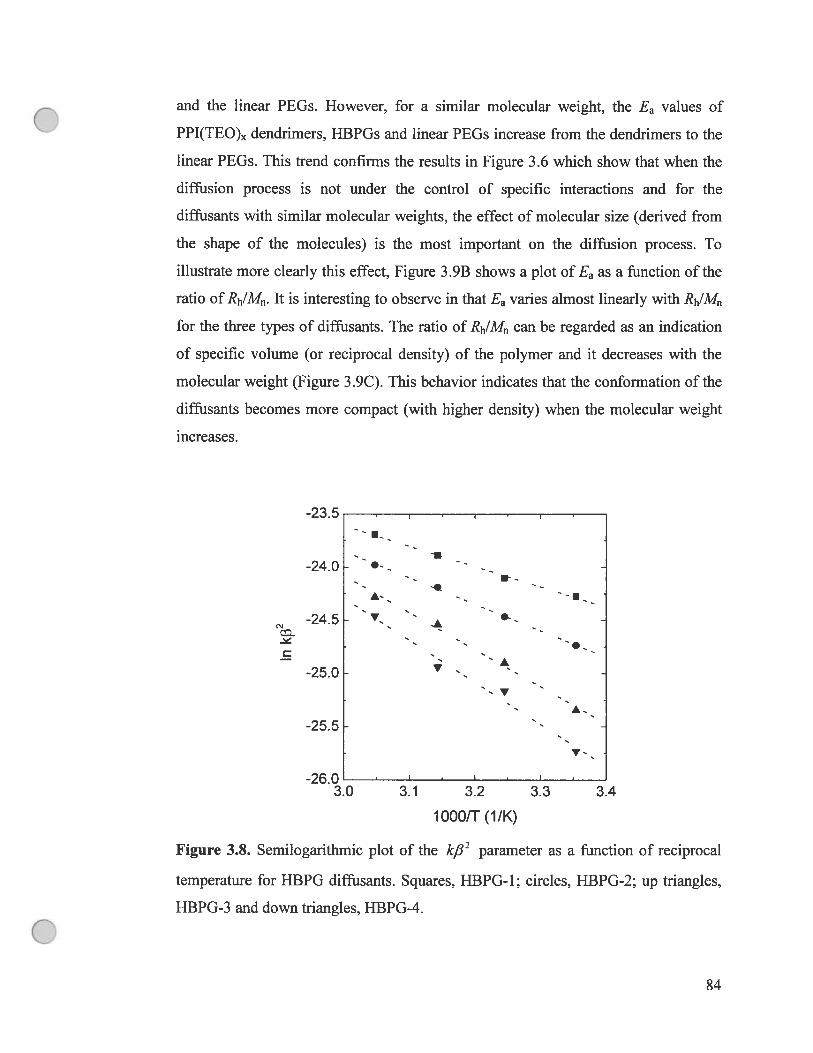
and the linear PEGs. However, for a similar molecular weight, the Ea values of

PPI(TEO) dendrimers, HBPGs and linear PEGs increase from the dendrimers to the

linear PEGs. This trend confirms the resuits in Figure 3.6 which show that when the

diffusion process is not under the control of specific interactions and for the

diffusants with similar molecular weights, the effect of molecular size (derived from

the shape of the molecules) is the most important on the diffusion process. To

illustrate more clearly this effect, Figure 3.9B shows a plot of Ea as a function of the

ratio of Rh/Mn. It is interesting to observe in that Ea varies almost linearly with Rh/M

for the three types of diffusants. The ratio of Rh/M can be regarded as an indication

of specific volume (or reciprocal density) of the polymer and it decreases with the

molecular weight (Figure 3.9C). This behavior indicates that the conformation of the

diffusants becomes more compact (with higher density) when the molecular weight

increases.

-23.5u

-24.0

-24.5-

C ,. .. -.

—

-25.0 V ..

À..

-25.5

-26.03.0 3.1 3.2 3.3 3.4

1000/1- (11K)

Figure 3.8. Semilogarithmic plot of the kfl2 parameter as a function of reciprocal

temperature for HBPG diffusants. Squares, HBPG-l; circles, HBPG-2; up triangles,

HBPG-3 and down triangles, H3PG-4.

84

50

À

À

ÀoE

3Q...

wÀ

20• A

100 5 10 15 20

M (x103 g/mol)50

10...

Rh/M (xl O i3nm*mol/g)

2.0À

À

1.5. CEEC

1.0

X.

0.5À

0.00 5 10 15 20

M (x103 g/mol)

Figure 3.9. (A) Variation of the apparent activation energy (Fa) obtained from the

k132 parameter as a function of the molecular weight (Ma) of the diffusants. (B)

Variation of Fa as a function of the ratio of Rh/M. (C) Variation of Rh/M as a

function of M of the diffusants. Squares, poly(propylene-imine) dendrimers; circles,

C) HBPG-4; triangles, linear PEG. The unes are drawn as visual guides.

$5

Figure 3.9C aiso shows that, for similar molecular weight, the density of the

molecules follows a order from PPI(TEO) dendrimers to HBPGs and then to linear

PEGs. At a very high density (when RhIM becomes very small), the three kinds of

diffusants approach a similar value of apparent activation energy. Extrapolation to

Rh/M to O gives Ea values of 45 ± 2, 47 ± 8 and 48 ± 7 kJ/mol for PPI(TEO)

dendrimers, HBPGs and PEGs, respectiveiy.

3.5. Conclusion

It is clearly shown that the self-diffusion coefficients of the HBPG decrease

with increasing molecular size of the diffusant, with increasing PVA concentration,

but with decreasing temperature. These results show that for the same molecular

weight and at the same PVA concentration, the diffusion is mainly affected by the

size of the diffusant resuiting from the molecular shape when specific interactions are

not predominant. As expected, larger diffusing moiecuies need higher apparent

activation energy to diffuse in the polymer systems. for ail diffusants, the density

increases with the molecular weight and for the diffusants with similar molecular

weight the density increases from linear PEGs to HBPGs and then to PPI(TEO)

dendrimers. The qualitative value of the density distribution for the three kinds of

diffusants is different. The fractal dimension value (1IŒ) obtained for PPI(TEO)

dendrimers indicates that the density distributions are close to a compact space-filling

structure while the values of HBPGs are similar to those of swollen polymer chains

or polymers in good solvent. Furthermore, the density distribution of linear PEGs

corresponds to polymer cous in a 0-solvent.

The physical model of Petit et al. describes well the variation of the self-

diffusion coefficient with the molecular weight of the HBPG, the polymer

concentration and the temperature. However, the model in its present form does not

provide an adequate description of the effects of both size and shape of the diffusants

on the self-diffusion coefficient. Molecular weight alone cannot account for the size

effect. The shape of the diffusants, hence the molecular density distribution of the

diffusant, should be an important factor to be considered in the diffusion process.

C$6

Q3.6. Acknowledgments

The financial support from the Namral Sciences and Engineering Research

Council (N$ERC) of Canada is grateftilly acknowledged. The authors also thank Ms

H. Thérien-Aubin and Dr. C. Malveau for their help in selected NMR experiments.

3.7. References and Notes

[1] Bon, C. L.; Nicolai, T.; Kuil, M. E.; Hollander, J. G. I Phys. Chem. B 1999,

103, 10294-10299.

[2] Wisnudel, M. B.; Torkelson, J. M. Macromolecules 1996, 29, 6193-6207.

[3] Gao, P.; fagemess, P. E. Pharm. Res. 1995, 12, 955-964.

[4] von Meerwall, E. D. Adv. Polym. Sel. 1984, 54, 1-29.

[5] fujita, H. Adv. Polym. Sel. 1961, 3, 1-47.

[6] Yasuda, H.; Lamaze, C. E.; Ikenberry, L. D. Makromol. Chem. 1968, 118, 19-

35.

[7] Vrentas, J. S.; Duda, J. L. I Polym. Sel., Polym. Phys. Ed. 1977, 15, 403-416.

[8] Vrentas, J. S.; Duda, J. L. I Polym. Sci., Polym. Phys. Ed. 1977, 15, 4 17-439.

[9] Phillies, G. D. J. Macrornolecules 1986, 19, 2367-2376.

[10] Vrentas, J. S.; Vrentas, C. M. Macromotecules 1994, 27, 4684-4690.


29,6031-6036.

[12] Amsden, 3. MacromolecuÏes 1998, 31, 8382-8395.

[13] Masaro, L.; Zhu, X. X. Prog. Polym. Sel. 1999, 24, 73 1-775.

[14] Storey, R. F.; Mauritz, K. A.; Cox, 3. D. MacromoteeuÏes 1989, 22, 289-294.

[151 Mauritz, K. A.; Storey, R. F.; George, S. E. MaeromoÏeeules 1990, 23, 441-

450.

[16] Von Meerwall. E. D; Skowronski, D.; Hariharan, A. Macromolecules 1991,

G23, 2441-2449.

[171 Yu, W.; von Meerwall, E. D. Maeromoteeules 1990, 23, 882-889.

87

[18] Zhu, X. X.; Macdonald, P. M. MacromolecuÏes 1992, 25, 4345-435 1.

[191 Zhu, X. X.; Wang, F.; Nivaggioli, T.; Winnik, M. A.; Macdonald, P. M.

Macromotecules 1993, 26, 6397-6402.

[20) Petit, J.-M.; Zhu, X. X.; Macdonald, P. M. Macromolecules 1996, 29, 70-76.

[21] Masaro, L.; Zhu, X. X.; Macdonald, P. M. Macromolecules 1998, 3], 3880-

3885.

[22] Masaro, L; Ousalem, M.; Baille, W. E.; Lessard, D.; Zhu, X. X.

Macromotecules 1999, 32, 43 75-43 22.

[231 Masaro, L.; Zhu, X. X. Macromotecules 1999, 32, 5383-5390.

[241 Baille, W. E.; Malveau, C.; Zhu, X. X.; Kim, Y. H.; ford, W. T.

Macromolecules 2003, 36, $39-$47.

[25] Salazar, R.; Fomina, L.; fomine, S. Polym. BuiL, 2001, 47, 15 1-158.

[26] Sunder, A.; Hanselmann, R.; frey, H.; Mulhaupt, R. Macromolecules, 1999,

32, 4240-4246.

[27] Mandai, H.; Hay, A. S. Polymer 1997, 38, 6267-6271.


[29] Callaghan, P. T.; Trotter, C. M.; Jolley, K. W. I Magn. Reson. 1980, 37, 247-

259.

[30] Stilbs, P. Prog. NucÏ. Magn. Reson. $pectrosc. 1987, ]9, 1-45.

[31] Price, W. S. Concepts Magn. Reson. 1997, 9, 299-336.

[32] Miils, R. I Phys. Chem. 1973, 77, 685-688.

[33] Tomlinson, D. J. Mol. Phys. 1972, 25, 735-738.

[34] Amman, C.; Meier, P.; Merbach, A. E. I Magn. Reson. 1982, 46, 3 19-322.

[35] Pasch, H.; Schrepp, W. MALDI-TOF Mass $pectrometry of $ynthesis

Polymers, Springer-Verlag, Berlin Heidelberg, 2003.

[36] Tokar, R.; Kubisa, P.; Penczek, S. Macromolecules 1994, 27, 320-322.

88

[37] Vandenberg. E. J. J PoÏym. Sci., Polym. Chem. Ed. 1985, 23, 951-970.

[38] frey, H.; Hi5lter, D. Acta polym. 1999, 50, 67-76.

[39] Hanselmann, R.; H51ter, D.; frey, H. Macromolecules 1998, 31, 3790-3801.

[40J Waldeck, A. R.; Kuchel, P. W.; Lennon, A. J.; Chapman, B. E. Prog. Nitcl.

Magn. Reson. Spectrosc. 1997, 30, 39-68.

[41] Rietveld, I. B.; Bedeaux, D. Macromolecules 2000, 33, 7912-7917.


Hadjichristidis, N. Macromolecules 1993, 26, 4324-4331.

[43] Flory, P. J. Principles ofPolymer Chemistry, Corne!! University Press, Ithaca,

N.Y., 1953.

[44] Flory, P. J. J Am. Chem. Soc. 1941, 63, 3083, 3091, 3096.

[45] Pickup, S.; Blum, F. D. Macromolecules 1989, 22, 3961-3968.

[46] Stancik, C. M.; Pople, J. A.; Trolisâs, M.; Lindner, P.; Hedrick, J. L.; Gast, A.

P. Macrornolecules 2003, 36, 5765-5775.

[47] Scherrenberg, R.; Coussens, B.; Van Viiet, P.; Edouard, G.; Brackman, J.; De


[4$] PUtz, M.; Kremer, K.; Everaers, R. Phys. Rev. Lett. 2000, 84, 298-301.

[49] King, S. M. Modem Techniques for Polymer Characterization, John Wiley &

Sons, New York, 1999.

[50] Geladé, E. T. F.; Goderis, B.; De Koster, C. G.; Meijerink, N.; Van Benthem,

R. A. T. M.; fokkens. R.; Nibbering, N. M. M.; Mortensen, K.

MacromoÏecuÏes 2001, 34, 3552-3558.

[51] De Gennes, P. G. Scaling Concepts in Polymer Physics; Corneli University


[52] Peppas, N. A.; Lustig, S. R. HydrogeÏs in Medicine and Pharmay Vol. I:

Fundamentais, Boca Raton, Fia. CRC Press, c1986-c1987 Chap 3.

G$9

Q[53] Schaefer, D. W.; Han, C. C. Dynamic Light Scattering and Velocimetry.

Applications of Photon Corretation Spectroscopy Pecora, R., Ed., Plenum

Press, New York, 1982.

[54] Horkay, f.; Burchard, W.; Geissier, E.; Hecht, A.-M. M. MacromolecuÏes

1993, 26, 1296-1303.

[55] Horkay, f.; Burchard, W.; Geissier, E.; Hecht, A.-M.; M. Makromot. Chem.

MacromoL Symp. 1993, 76, 145-154.

[56] Wang, B.; Mukataka, S.; Kodama, M.; Kokufuta, E. Langmuir 1997, 13,

6102-6114.

[57] Wang, B.; Mukataka, S.; Kokufuta, E.; Ogiso, M.; Kodama, M. I Polym. Sci.

2000, 38, 214-221.

[5$] Peppas, N. A. Hydrogels in Medicine and Pharmay Vol. II: Polymers. Boca

Raton, fia., CRC Press, c1986-c1987, Chap. 1.

o90

Chapitre 4

Study of Diffusant-Polymer Matrix Interactions

by PFG NMR $pectroscopy

W. E. Baille, L Masaro, M. Gauthier, X. X. Zhu I Polym. $ci. Polym. Phys. 2004, à

soumettre.

4.1. Abstract

Pulsed-field gradient NMR spectroscopy was used to study the interactions

between diffusants and polymers. The self-diffusion coefficients of small diffusants

containing terminal hydroxyl, amine, carboxylic acid and aikyl groups have been

determined in several polymer matrices. Polymers matrices included poly(vinyl

alcohol), poly(N,N-diethyl acrylamide), poly(allylamine) and poly(acrylic acid)

which contain lateral hydroxyl, amine, carboxylic acid and amide groups. Resuits

show that the functional groups have a pronounced effect on the diffusion process.

for example, the self-diffusion coefficients measured in a poly(vinyl alcohol) matrix

are higher for the diffusants with carboxylic acid groups despite the fact that the

molecular weights of ail the diffusants are similar. This functional group effect has

been attributed to diffusant-polymer interactions. We have also studied the effect of

functionai groups of the polymers on the diffusion process and the effect of

temperature. The diffusion models of Petit et al. and of Phillies have been used to

interpret the data. These two models fit well to the experimental data even through no

provisions are available for the description ofthe interactions.

92

4.2. Introduction

The study of the diffusion of molecules in polymer matrices and biological

systems is of both fundamental and applied importance [1-12]. for example, in

search of an efficient controlled release system for drugs, it is fundamental to

understand the physical properties of the drug and of the matrix involved in the

diffusion process. The self-diffusion in polymer matrices has been studied using

pulsed-field gradient NMR spectroscopy [1-5, 13-19]. These studies include the

evaluation of the effect of the molecular weight, size and shape of the diffusants,

concentration of the polymer, solvent conditions, temperature and diffusant-polymer

interaction on the diffusion process [1-5, 13-19]. However, the effect ofthe chemical

diffusant/polymer interactions has flot been characterized as well as the other effects.

Some interesting studies show that diffusant-polymer interactions such as Coulombic

interactions and hydrogen bonding can reduce substantially the diffusion of a solute

[19-29]. For a polymer weight fraction of 0.06, the normalized self-diffusion

coefficient (D/Do) of 4-[[4-(dimethylamino)phenyl]azo]benzoic acid (usually named

p-methyl red) decreases from polystyrene (PS) (D/D0 = 0.8) to poly(methyl

methacrylate) (PMMA) (D/Do = 0.5) and then to poly(vinyl acetate) (PVAc) (D/Do

0.4) (these values have been extrapolated ftom the results of Lee and Chang) [29].

The decrease in D is strongly related to the availability of carbonyl group on PVAc to

participate in hydrogen bonding versus PS and PMMA [29].

Interactions such as hydrogen bonding have a significant effect on molecular

transport in polymer or biological systems [11, 12]. However, the influence of such

interactions on diffusion is not easily described given that hydrogen bonding is space

dependent (dependent upon the spatial configuration of the atoms participating in the

interaction). The space dependence implies that subtle structural differences among

the diffusants can significantly alter these specific interactions [30].

The aim of the present study is to evaluate the self-diffusion coefficients of a

series of small diffusants by pulsed field gradient NMR spectroscopy in order to

illustrate the effect of hydrogen bonding on the diffusion process in polymer

solutions and gels. This report also includes the effects of functional groups on the

diffusants and on the polymer matrix and the effect of temperature on the

93

interactions.


4.3.1. Materials

Ethylene glycol (EG), diethylene glycol (DEG), triethylene glycol (TEG) and

their end-capped methyl ether derivatives as well as ethylene diamine (EDA), acetic

acid tRAc) were purchased from Aldrich (Milwaukee, WI). Polymers such as

poly(vinyl acohol) (PVA), poly(allylamine) (PAAm) and poly(acrylic acid) (PAA)

were also purchased from Aldrich (Milwaukee, WI). D20 was purchased from C.I.L.

(Andover, MA). All chemicals were used as received. Poly(N,N-diethylacrylamide)

(PDEA) was prepared as described in our previous reports [31].

4.3.2. Sample Preparation

The NMR samples were prepared by a previously described method [13, 14,

16]. PVA (M = 52 000 with a degree of hydrolysis equal to 99 %), PDEA (M4 = 70

000), PAAm (M = 65 000) or PAA (M = 100 000) were added into D20 solutions

containing 1 wt% diffusant in 5.00 mm o.d. NMR tubes. The concentration of

polymers (c) ranged from O to 0.36 g/mL.

4.3.3. Pulsed Field Gradient NMR Measurements

The spin echo (SE: 90°-ti-1$0°-ti-echo) technique developed by Stejskal and

Tanner [32] and the stimulated echo (STE: 90°-ti-90°-t2-90°-ti-echo) technique

developed by Tanner [33] were used to measure the self-diffusion coefficients (D) of

solute probes. Measurements were performed on a Bruker DSX-300 NMR

spectrometer operating at a frequency of 300.1$ MHz for protons. The NMR

experiments for the determination of the self-diffusion coefficients have been

presented previously [14, 16]. The quality of the fitting to the experimental data is

also indicated by the good fits shown in all the figures. The root mean square

correlation coefficients (R2) were in the range of 0.990 - 0.999. Identical sets of

fitting parameters were obtained regardless of the initial values used in the procedure.

The experiments were performed at 5 different temperatures (from 25 to

45°C) (fluctuation ± 0.3°C) and polymer concentration ranged from O to 0.36 g/mL.

Temperature calibration was done periodically as described previously [16].

94

4.4. Resuits and Discussion


The diffusant/polymer interaction process was investigated by measuring the

self-diffusion coefficients of several diffusants containing terminal hydroxyl,

carboxylic acid, amine and amide groups, into four different polymer matrices,

shown in Figure 4.1.

[ CH2_CH_}_ { CH2_CH_]_

OH COOH

Poly(vinyl acohol) (PVA) Poly(acrylic acid) (PAA)

[ CH2_CH_]_ [ cH2_CH_j_

CH2

NH2

Poly(allylamine) (PAAm) PoIy(N,N-diethylaciylamide) (PDEA)

Figure 4.1. $chematic structure of polymer matrices used to study diffusant!polymer

interactions.

4.4.1.1. Effect of Polymer Concentration

The effect of polymer concentration on the diffusant-polymer interaction

process was first evaluated by studying the diffusion of EG, DEG and TEG in PVA

solutions with increasing concentration of PVA. Figure 4.2 shows the expected

decrease in the self-diffusion coefficient with increasing PVA concentration. This has

been rationalized by separating the PVA solutions in two regions, separated by the

critical overlap concentration ofthe PVA solution (c and c = 7 wt% or 0.09 g/mL

as determined by rheology). Before c”, the increase of matrix viscosity associated

with polymer concentration makes the diffusion process more difficult.

95

10

8

U)

2

[PVAJ (g/mL)

Figure 4.2. Variation of the self-diffusion coefficients as a function of PVA

concentration at 25 °C. Dashed unes are fits to eq 4.3. Squares, EG; circles, DEG;

and triangles, TEG.

Afier e , increasing polymer concentration leads to the formation of a network

characterized by a correlation length, regarded as the average mesh size of the

network [34]. Thus, decreases rapidly with increasing polymer concentration due to

the contact and entanglement of the polymer chains [35, 36]. This in tum makes it

harder for the diffusants to pass through the network. Despite the change in the

polymer concentration regime, the value of the self-diffusion coefficient decreases

steadily with the concentration of PVA and no abrupt changes are observed even with

this change of regime. Generally, a drastic change is observed for certain polymer

solution properties when e c. For example, at e ? e a strong increase of the

viscosity ofthe polymer solution is observed [37, 38].

4.4.1.2 Effect of Diffusant Molecular Weight

Figure 4.2 illustrates the decrease in D with the molecular weight of the

diffusants, i. e., EG, DEG and TEG. The effect of molecular weight on the diffusion

o0.0 0.1 0.2 0.3 0.4

96

process has been described by the use ofthe Stokes-Einstein equation [391:

D0 = kBT(4.1)

62r77Rh

where D0 is the self-diffusion coefficient in the absence of the polymer, k8 is

Boltzmann’s constant, and Rh is the effective hydrodynamic radius of the diffusing

molecule, which is related to Ï7and Mby the following expression [39]:

Rh=3/3M

(4.2)t14,r N

where Mis the molecular weight of the diffusant, V is the experimentally determined

partial specific volume ofthe diffusing molecule, and N is Avogadro’s number. From

eq 4.2, D0 must be inversely proportional to the cubic root of the molecular weight

when the diffusant is a hard sphere. If the diffusants in Table 4.1 are hard spheres a

graph of D0 as a function of M113 should be linear. figure 4.3 shows the resuits

obtained for the diffusants studied here. The profile indicates that these diffusants

may be regarded as hard spheres. This proportionality is also valid when the diffusion

process is not affected by the interactions between the diffusant and its surroundings.

The effect of molecular weight can also be explained by the free volume theory [40-

43]. This theory suggests that the diffusion process is controlled by the formation of

adjacent free volume large enough to allow the diffusant to move from its present

void into the next. With increasing molecular size (molecular weight being related to

the molecular size), the adjacent void required for the diffusion to take place must be

larger. This would lead to a reduced diffusion rate.

Dashed unes in figure 4.2 represent the result of the fit to the model of Petit

et al. [44]:

DD0

2v (4.3)1+ ac

97

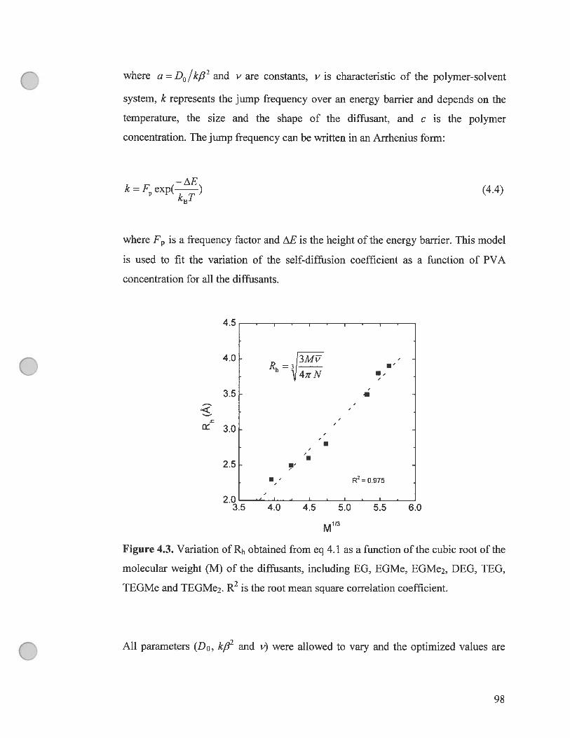
where a = D0 /kfl2 and y are constants, y js characteristic of the polymer-solvent

system, k represents the jump frequency over an energy barrier and depends on the

temperature, the size and the shape of the diffusant, and e is the polymer

concentration. The jump frequency can be written in an Arrhenius form:

k = f exp(E) (44)

where F is a ftequency factor and AE is the height of the energy barrier. This mode!

is used to fit the variation of the self-diffusion coefficient as a function of PVA

concentration for ail the diffusants.

4.5 I I I

4.0 13MVR 3!

4,zN B’

3.5

3.0 -,

.2.5

R2=O.975

2.0 — ‘ I I

3.5 4.0 4.5 5.0 5.5 6.0

M113

Figure 4.3. Variation of Rh obtained from eq 4.1 as a function ofthe cubic foot ofthe

molecular weight (M) of the diffusants. including EG, EGMe, EGMe2, DEG, TEG,

TEGMe and TEGMe2. R2 is the foot mean square correlation coefficient.

Ail parameters (D0, kfl2 and y) were allowed to vary and the optimized values are

9$

listed in Table 4.1. The fitted values of D0 show excellent agreement with those

measured by the NMR experiments. As expected, D0 and kfl2 decrease with

molecular weight. The value of y is expected to be a constant within a certain range

but experirnental resuits indicate that it shows a slight decreasing trend with the

molecular weight of the diffusant. However, the values of y remain in the range of

0.49 to 0.76 with an average of ca. 0.58 as obtained previously for other diffusants in

the same polymer-solvent system under identical conditions [13, 14, 16]. Table 4.1

also reports the effective hydrodynamic radius (Rh) obtained for EG, DEG and TEG

from the Stokes-Einstein equation (eq 4.1).

Tab]e 4.1. Self-diffusion coefficients (D0), hydrodynamic radii (Rh) and fitting

parameters kfi2 and vobtained in aqueous PVA systems

D0 (1 0’°m2/s) ta) (a) Rh” R2(c)

Samples

exp. calc.a (10’° s/m2) (À)

EG 8.7 ± 0.2 8.6 ± 0.1 0.98 ± 0.06 0.62 ± 0.02 2.3 0.998

EGMe 7.9±0.1 7.8±0.2 1.17±0.05 0.60±0.02 2.5 0.999

EGMe2 7.6 ± 0.3 7.6 ± 0.2 1.27 ± 0.0$ 0.56 ± 0.02 2.6 0.99$

DEG 7.3 ± 0.2 7.2 ± 0.2 0.44 ± 0.05 0.65 ± 0.04 2.7 0.995

TEG 5.7 ± 0.3 5.6 ± 0.2 0.21 ± 0.04 0.72 ± 0.04 3.5 0.992

TEGMe 5.2 ± 0.1 5.2 ± 0.2 0.65 ± 0.03 0.5$ ± 0.02 3.$ 0.999

TEGMe2 5.1 ± 0.2 5.1 ± 0.1 0.64 ± 0.05 0.58 ± 0.02 3.9 0.997

(a)obtajfled as a fitting parameter from eq 4.3.

(b)calculated from eq 4.1.

tc)root mean square correlation coefficients

99

4.4.1.3 Diffusant-Polymer Interaction

Figure 4.2 and the parameters D0 and kfl2 listed in Table 4.1 for EG, DEG

and TEG illustrate the expected decrease of the self-diffusion coefficient with the

molecular weight of the diffusants. However, the normalized self-diffusion

coefficients of EG, DEG and TEG as a function of PVA weight fractions (Ø) clearly

show that the diffusion process of these diffusants is also affect by the interactions

between the diffusant and the PVA matrix (Figure 4.4).

I I I I

1.0 ê

“u0.8

,*, \0.6

D 4.

I...0.4. ........—..

À..

0.2.

0.0’0.0 0.1 0.2 0.3 0.4

Figure 4.4. Dependence of D/D0 as a function of PVA weight fraction () at 25 oc.

Dashed unes are fits to eq 4.5. Squares, EG; circles, DEG; and triangles, TEG.

In our case, the dominant interaction is hydrogen-bonding between the

diffusants and the PVA matrix. Figure 4.4 also shows that the effect of hydrogen

bonding is more efficient in the retardation of the diffusion process of TEG versus

DEG or EG. This behaviour is probably due to the greater number of oxygen atoms

available to participate in hydrogen bonding on TEG (4 oxygen atoms) versus DEG

(3 oxygen atoms) and EG (2 oxygen atoms).

To quantitatively characterize the interactions between the diffusant and the

100

polymer, the well established stretched exponentiai form of Phillies has been used

[45, 46].

D/D0 =exp(_açY) (4.5)

where a and u are constants which depend on the system of interest [22, 29, 45, 46].

However, many papers in the literature define a as a constant related to the molecular

weight of diffusants (u M’ in the case of macromolecule diffusants and t is a

constant), whereas Œ depends on the hydrodynamic radius of the diffusant (u = aR

where a and b are constants with value between 3.03-3.20 for a and 0.53-0.59 for b)

for smaller diffusants [2, 22, 43]. According to Lee and Chang, the parameter u can

be used to distinguish the diffusion process retarded by hydrogen-bonding from the

one retarded by hydrodynamic interactions (dependence of D on polymer

concentration) [27]. Lee and Chang found y equal to 0.62 ± 0.06 and 1.0 ± 0.1 fora

diffusion process controlled by hydrogen-bonding and hydrodynamic interactions,

respectively [27].

This model is used to fit the variation ofD/D0 versus for the three diffusants

as iliustrated in Figure 4.4. Ail parameters (u and y) were ailowed to vary and the

optimized values are listed in Table 4.2. The values of u obtained by this fitting

method do flot show a clear dependence on the hydrodynamic radius of the

diffusants. Moreover, the parameter u cannot be used to illustrate the interactions

between the diffusant and the polymer shown in Figure 4.4. The values of y obtained

for EG, DEG and TEG indicate that hydrodynamic interactions have a major effect

on the diffusion process. However, Figure 4.4 shows that the diffusion of EG. DEG

and TEG into the PVA matrix is affected by interactions such as hydrogen-bonding.

The stretched exponential form (eq 4.5) does not provide an appropriate description

of the interactions between the diffusant and the polymer.

b study the effect of hydrogen-bonding between EG, DEG and TEG

diffusants and the PVA on diffusion, the self-diffusion coefficients ofthese diffusant

101

were compared with their end-capped methyl ether derivatives. figure 4.5A shows an

example of resuits obtained for TEG, TEGMe, and TEGMe2 diffusants. One notices

that the difference between the self-diffusion coefficients of TEG and its end-capped

methyl ether derivatives is insignificant at lower PVA concentrations.

Table 4.2. Fitting parameters values of a and y obtained in aqueous PVA

systems by the use of eq 4.5

Samples (a) 4) a(b) R (c)

EG 2.3 3.6±0.1 0.89±0.02 1.000

EGMe 2.5 3.1±0.1 0.90±0.03 0.999

EGMe2 2.6 2.$ ± 0.1 0.83 ± 0.03 0.998

DEG 2.7 5.0±0.1 0.89±0.01 1.000

TEG 3.5 6.7 ± 0.4 0.97 ± 0.03 0.999

TEGMe 3.8 3.3 ± 0.2 0.84 ± 0.03 0.998

TEGMe2 3.9 3.3 ± 0.1 0.84 ± 0.03 0.999

fa) calculated from eq 4.1.

(b)obtained as a fitting parameter from eq 4.5.

(c)root mean square correlation coefficients

This difference becomes more significant at higher PVA concentration despite the

fact the TEGMe and TEGME2 have molecular weights higher than TEG. The

difference in D between these two diffusants is within experimental error (less than

5%). A doser examination of the curves of TEGMe and TEGMe2 reveals that the

values ofthe self-diffusion coefficients are systematically bigher for TEGMe than for

TEGMe2. The molecular weight effect of the diffusant is also insignificant when the

self-diffusion coefficients of EG and DEG are compared with their end-capped

methyl ether derivatives (data flot shown).

102

U)

E

b

0.8

0.6

0.4

0.2

0.00.0 0.1 0.2 0.3 0.4

0.0 0.1 0.2 0.3 0.4

1.0

0.8

0.6

0.4

0.2

[PDEA] (g/mL)

0.0 0.1 0.2 0.3 0.4

Figure 4.5. Variation of the self-diffusion coefficients as a function of (A) PVA and

(B) PDEA concentrations at 25 °C. Dashed unes are fits to eq 4.3. Dependence of

D/Do as a function of (C) PVA and (D) PDEA weight fractions (4) at 25 °c. Dashed

unes are fits to eq 4.5.

The absence of the molecular weight effect illustrated in Figure 4.5A could be the

resuit of hydrogen bonding interactions between the diffusants and the polymer since

the self-diffusion coefficients were measured under the same experimental conditions

and that the presence of methyl ether groups should not significantly alter the shape

5

4

3

C

N•TEG• TEGMeÀ TEGMe

2

[PVA] (g/mL)

n

1.0

B

• TEG• TEGMeÀ TEGMe

1

h..

D

• TEG• TEGMeÀ TEGMe

103

of the diffusant (Table 4.1, size of diffusants, R h), which is known to affect diffusion

[16, 17]. The interaction between EG and the PVA matrix has been illustrated

previously by the use of ‘H NMR spectroscopy [19]. It was shown that when PVA

was added to EG-D20 solutions, an additional signal was observed which was found

to correspond to EG bound to the PVA matrix [19].

The physical model of Petit et al. was also used to fit the diffusion profiles

illustrated in figure 4.5A. The resuits of the fitting parameters are listed in Table 4.1

which also contains the fitting parameters for EGMe and EGMe2. One notices that

the D0 values obtained by fitting and by NMR experiments show a clear molecular

weight dependence for both series of diffusant (EG, EGMe, EGMe2, TEG, TEGMe

and TEGMe2). When the kfl2 parameter is examined, an opposite trend, albeit small,

with the molecular weight is observed. In fact, the physical definition of the k/2

parameter implies that it should decrease with increasing molecular weight. It is

known that when the diffusion process is affected by the interactions between the

diffusant and the polymer or the diffusant shape, the k/32 parameter may follow an

opposite trend with increasing molecular weight [16, 17]. The resuits obtained for the

kfl2 parameter from Figure 4.4 and 4.5A show that the model of Petit et al. is

incapable of illustrating the interactions between the diffusant and the polymer when

we compare diffusants with different molecular weight. In this case, a realistic

interpretation of the resuits of the fitting process can be done only as a function of

molecular weight. However, Figure 4.4A clearly shows that the diffusion process of

TEG as well as EG and DEG (data flot shown for EG and DEG) is significantly

influenced by hydrogen bonding between the diffusant and the polymer. Resuits

obtained by fitting to the model of Petit at al. indicate that the kfl2 parameter may be

used to describe the interactions between the diffusant and the polymer only when

chemical interactions (for example hydrogen bonding and Coulombic interactions)

are the dominant factor affecting the diffusion process. The model in its present form

does flot provide an adequate description of the chemical interactions between the

diffusant and the polymer. This affirmation is based on the fact that the k2

parameter changes with the molecular weight of the diffusant, the temperature, the

shape of the diffusant and the interactions between the diffusant and the polymer.

104

This model remains useful for analyzing the experimental diffusion data. Conceming

the parameter t the resuits in Table 4.1 are in the same range as those obtained in

previous studies (0.49 to 0.76 with an average ofca. 0.5$) [13-1$].

The hydrogen bonding between TEG and the PVA matrix can be also

illustrated if the values of the normalized self-diffusion coefficients of TEG and its

end-capped methyl ether derivatives are plotted as a function of PVA matrix

concentrations. Figure 4.5B shows the resuits obtained for D/D0 in PVA matrix.

from Figure 4.5B it is clear that TEG interacts chemically with the PVA matrix but

in the case TEGMe and TEGMe2, hydrodynamic interactions are the dominant factor

retarding the diffusion process.

To clearly put out the effect of the interactions between the diffusant and the

polymer on diffusion, the self-diffusion coefficients of EG, DEG, TEG, and their

end-capped methyl ether derivatives were determined in a different polymer matrix

(PDEA). As illustrated in figure 4.1, PDEA has lateral amide groups and thus

interacts to a lesser extent with the diffusants. It is hypothesized that the presence of

the ethyl groups linked to the nitrogen atom reduces considerably the possibility of

hydrogen bonding between the nitrogen atom and the hydroxyl groups on EG, DEG

and TEG. However, in the case of PVA, the availability of hydroxyl groups (with a

degree of hydrolysis of 99%) enhances the probability of hydrogen bonding. figure

4.5C shows the resuits obtained for TEG and its end-capped methyl ether derivatives.

The diffusion process of TEG and its end-capped methyl ether derivatives is clearly

affected by the molecular weight of the diffusant. As expected in absence of

hydrogen bonding or Coulombic interactions, the diffusant with the higher molecular

weight has a lower self-diffusion coefficient. Moreover, the molecular weight effect

is independent of the polymer matrix concentration. The difference observed in the

self-diffusion coefficient is proportional to the difference in the molecular weight of

the diffusant. The effect of molecular weight has also been examined for EG, DEG,

and their end-capped methyl ether derivatives (data flot shown). The dashed unes in

figure 4.5C are the resuit of the fit with the model of Petit et al. and the value for

each parameter is presented in Table 4.1. Contrary to the k,82 values obtained for the

diffusion process of TEG and its derivatives in PVA matrix (see Table 4.1), the

105

resulting kfi2 va’ues in the PDEA matrix tend to decrease when the molecular weight

ofthe diffusant increases. For example. we have obtained kfl2 values of 0.79 x 100,

0.67 x 1W1° and 0.64 x 10b0 s/m2 for TEG, TEGMe and TEGMe2, respectively, in a

PDEA matrix. This resuit also shows that without significant interactions between the

diffusant and the polymer or other effects, the jump frequency decreases with the

molecular weight. Consequently the apparent activation energy as illustrate in eq 4.4

should increase. The physical model of Petit et al. describes well the diffusion

process without chemical interactions between the diffusants and the PVA matrix.

In the same way, the resuits in Figure 4.5D show that the normalized self-

diffusion coefficients for these three diffusants follow the same trend and are seen to

faïl on the same une fitted with eq 4.5. Within experimental error, these resuits

indicate that no other specific interaction is responsible for the retardation of self-

diffusion coefficient than the hydrodynamic interactions between the diffusants and

the PDEA matrix.

The dashed unes in Figure 4.5B and 4.5D are the result of the fit with the

stretched exponential form of Phillies (eq 4.5). As shown previously, the resuits

obtained for a and u do not indicate any clear hydrodynamic radius ta = aRs)

dependence or hydrogen-bonding (u equal to 0.62) effect [27]. for example, a

values obtained are 3.2, 3.4 and 3.3 for TEG, TEGMe and TEGMe2, respectively. In

the case of y, the values from the fitting method are 0.87, 0.92 and 0.87 for TEG,

TEGMe and TEGMe2, respectively. By comparing the values indicated in Table 4.2

for the diffusion process in PVA matrix to those in PDEA matrix, it appears that

hydrodynamic interactions are the dominant processes in both matrices. Thus,

explanation cannot be deduced by the use ofthese resuits.

4.4.1.4 Functional Group Effect

The investigation of the effect of flmctional groups on the diffusion process

was done by the use of EG, EDA and HAc as diffusants. The three diffusants have

similar molecular weight (MEG 62.1, MEDA = 60.1 and MFtA = 60.1) but have

different functional groups. Figure 4.6A shows resuits obtained for these diffusants in

a PVA matrix. Despite their similar molecular weights, D0 values of 8.3 x 100 m2/s

106

and 10.1 x 10° m2Is were obtained for EDA and HAc, respectively.

12

u)

Eo

ots

D

0.8

oDD

0.4

0.2

0.0 0.1 0.2 0.3 0.4

Figure 4.6. (A) Change of the self-diffusion coefficients for three diffusants (EG,

EDA and HAc) with similar molecular weight as a function of PVA concentration at

25 °C. Dashed unes are fits to eq 4.3. (B) Dependence ofD/D0 as a function ofPVA

weight fraction () at 25 °C. Dashed unes are fits to eq 4.5. Squares, EG; circles,

EDA; and triangles, HAc.

0.2[PVA] (g/mL)

1.0B

1

“t’

5.,j,

107

This difference (1$ %), is roughly four times the experimental error estimated by

carrying out repeated experiments. Furthermore, the D0 values of EG and EDA are

similar (8.7 x 10b0 m2/s for EG and 8.3 x 10b0 m2/s for EDA with a difference of 5

%). The difference or the similarity of the D0 values for these diffusants can be an

effect of Brønsted acids and bases. It is known that HAc is partially ionized (HAc(l)

+ H20(l) ÷-÷ H3O(aq) + Ac(aq) where 1 indicates a liquid state and aq is an

abbreviation of aqueous solution) and the molar conductivity (Am) of H at a

concentration of HAc higher than 0.03 mol/L is significantly lower than the one at

infinite dilution [30]. For example, Am is inferior to 20 $cm2/mol at a concentration

ofllAc higher than 0.03 mol/L but Am is superior to 390 $cm2/mol at infinite dilution

[30]. This lower value 0f Am at a concentration of FlAc higher than 0.03 mol/L can be

an indication of a disordered arrangement of water molecules (an anti-Grotthuss

arrangement of water) which can also indicates that Ac anion has a higher mobility.

This can explained the higher self-diffusion values obtained for HAc in comparison

to EG and EDA. figure 4.6A shows the difference (or similarity) ofthe self-diffusion

coefficients of the three diffusants in PVA matrix. This figure shows that the

presence of the polymer does flot change the difference or the similarity of the self-

diffusion coefficient obtained at zero concentration of polymer. Fitting the

experimental data with the model of Petit et al. yields k2 values of 0.9$ x 1 0b0, 1.04

x 10° and 1.54 x 1OE1° s/m2 for EG, EDA, and HAc, respectively. These values

indicate that the diffusion process may be easier for HAc with a lower activation

energy than for EG or EDA. Figure 4.4 has shown the presence of hydrogen bonding

between EG and the PVA matrix, to verify that kind of interactions for EDA and

HAc the values D/D0 versus b have been plotted (figure 4.6B). The first look of

figure 4.6B shows that the data points of ah diffusants follow the same trend which

indicates that no chemical interactions are existed between the diffusant and the

polymer. However, a comparison with the results show in Figures 4.4 and 4.5 allows

us to said that the Figure 4.63 indicates that the interactions between the diffusant

and the polymer exist but the magnitude of these interactions are similar for EG,

EDA and HAc. It is also clear from Figure 4.6 if the chemical interactions between

these diffusants and the polymer exist but the dominant factor influencing the

10$

u)

Eo

b

o

diffusion process largely the effect ofBrønsted acids and bases.

[PVAJ (g/mL)

-21.5

B

•EG

À • EDAÂHAc

•‘• -À

À.

s.

-22.0

-22.5

-23.0

3.1 3.2 3.3 3.4

1000/T (11K)

Figure 4.7. (A)Variation of the self-diffusion coefficients of the EG as a function of

PVA concentrations at five different temperatures. Dashed unes are fits to eq 4.3. (B)

$emilogaritbmic plot of the k/32 parameter as a function of reciprocal temperature

for the tbree diffusants.

109

Thus, the difference on the D0 despite the similar molecular weight is caused

probably by the fact that the interaction of EG et EDA with the solvent is stronger

than HAc which suppose that the apparent activation energy of self-diffusion should

5e similar for EG and EDA. The effect of the temperature was studied between 25

and 45°C. Typical resuits are shown in Figure 4.7 for the variation of the self-

diffusion coefficient of EG with PVA concentration (from O to 0.3$ g/mL) at 5

different temperatures. As previously illustrated, D increases with increasing

temperature [14-17]. The apparent activation energy for each diffusant has been

obtained using the variation of k/32 parameter with the reciprocal temperature such as

the Arrhenius approach (Figure 4.7B). $ince we assume that fi is a constant within

the temperature range studied here, the variation of kfi2 with the temperature reflects

the variation of k as a function of temperature. A good linear relationship is obtained

for these three diffusants. The apparent activation energy values obtained ftom the

variable temperature experiments in a PVA matrix are 33.7, 34.1 and 26.6 kJ/mol for

EG, EDA and HAc, respectively. As expected, these values indicate that T-TAc

requires less activation energy than EG and EDA to diffuse.

To prove that EG, EDA and HAc interact with the PVA matrix, the diffusion

process of these three diffusant have been studied in the four different polymer

matrices (PVA, PDEA, PAAm and PAA). In fact, diffusion studies ofEG, EDA, and

HAc in these polymer matrices have shown that at the same polymer concentration

the self-diffusion coefficients of HAc are rather similar in PVA and PAA but

decrease significantly in PAAm. For example, at a polymer concentration of 0.03

g/mL, the self-diffusion coefficient ofllAc is 8.7 x 10b0, 8.1 x 10°, and 5.8 x 10b0

m2/s in PVA, PAA and PAAm, respectively. Figure 4.8 shows an opposite trend for

the self-diffusion coefficients of EG in the same four polymer matrices. The value of

D for EDA was higher in PAAm than in PVA (for example at 0.03 g!mL of the

polymer concentration, the D values for EDA were 7.9 x 10b0 and 7.3 x 1010 m2/s,

respectively, in PAAm and PVA). The mechanism by which the functional groups

affect the diffusion process is not quite clear, but Amsden et al. reported that the

difference in the values of D versus functional group type is flot the resuit of the

molecular weight of the polymers because this effect may be observed when the Rh

110

U)

of the diffusant is higher than 250 À [47]. This change of D can be also attributed to

the difference in hydrogen bonding resulting from the functional groups of the

diffusant and the polymer. From Figure 4.8 it is clear that the interactions between

EG and each polymer matrix (PVA, PDEA, PAAm and PAA) are different. It is also

clear that these interactions are flot hydrodynamic interactions.

10

8

6

4

20.0

Figure 4.8. (A) The evolution of self-diffusion coefficients of EG into four polymer

matrices and at different polymer concentrations. Dashed lines are fits to eq 4.3.

4.5. Conclusion

We have studied the self-diffusion coefficients of small diffusants containing

terminal hydroxyl, amine, carboxylic acid, and aikyl groups in several polymer

matrices. In addition to the variation of self-diffusion coefficients (decrease with

increasing diffusant molecular size, with increasing polymer concentration, and with

decreasing temperature) the interactions between diffusant and polymer were found

to lower significantly the value of self-diffusion coefficient and consequently reduce

0.1 0.2

[Polymer] (g/mL)

111

considerably the effect of molecular size of the diffusants. The normalization D/D0

gives a better indication ofthese interactions.

The physica! model of Petit et al. describes well the variation of the self-

diffusion coefficient with diffusant size, polymer concentration, and temperature.

However, the description of the interactions between diffusant and polymer may be

possible when this effect is the dominant factor influencing the diffusion process.

Otherwise. the physical mode! in its present form does flot provide an adequate

description of the effect of chemical diffusant/polymer interactions on diffusion.

Results obtained show also that the stretched exponential form of Phillies (eq 4.5) is

flot adequate to describe the interactions observed between the diffusants (EG, DEG

and TEG) and the PVA matrix.

4.6. Acknowledgments.

The financial support from the NSERC of Canada and Canada Research Chair

Program are gratefu!ly acknowledged. M. A. Gauthier acknowledges graduate

research scholarships from N$ERC of Canada and fQRNT of Quebec.


[1] Brown, W.; Stilbs. P. I Appi. Polym Sel. 1984, 29, 823-827.

[2] Gibbs, S. J.; Johnson Jr.; C. S. Macrornolecules 1991. 24, 6110-6113.

[3] Zhu, X. X.; Macdonald, P. M. Macromolecules 1992, 25, 4345-435 1.

[4] Zhu, X. X.; Wang, f.; Nivaggioli, T.; Winnik, M. A.; Macdonald, P. M.


[5] Griffiths, P. C.; Stilbs, P.; Chowdhry, B. Z.; Snowden, M. J. CoÏÏoidPolyrn. Sel.

1995, 273, 405-411.

[6] Waggoner, R. A.; Blum, f. D.; Lang, J. C. Macromolecules 1995, 28, 2658-

2664.

[7] Storey, R. f.; Mauritz, K. A.; Cox, 3. D. Macromolecules 1989, 22, 289-294.

[8] von Meerwa!!, E. D; Skowronski, D.; Hariharan, A. MacromoÏecuÏes 1991, 23,

2441-2449.

112

[9] Yu, W.; von Meerwall, E. D. Macromolecules 1990, 23, $82-$89.

[10] Liu, M.; Nicholson, J. K.; Lindon, J. C. Anal. Commun. 1997, 34, 225-228.

[11] Le Bon, C.; Nicolai, T. I Phys. Chem. B 1999, 103, 10294-10299.

[12] Schoberth, S. M.; Bar, N.-K.; Kramer, R.; Karger, J. Anal. Biochem. 2000, 279,

100-105.

[13] Petit, J.-M.; Zhu, X. X.; Macdonald, P. M. Macromolecules 1996, 29, 70-76.

[14] Masaro, L.; Zhu, X. X.; Macdonald, P. M. Macromolecules 1998, 3], 3280-

3885.

[15] Masaro, L.; Zhu, X. X. Macromolecules 1999, 32, 53 83-5390.

[16] Baille, W.E.; Malveau, C.; Zhu, X.X.; Kim, Y.H.; ford, W.T. Macromolecules

2003, 36, $39-$47.

[17] Baille, W.E.; fomine, S.; Zhu, X.X. Macromolecules 2004, 37, 8569-8576.

[1$] Masaro, L.; Ousalem, M.; Baille, W. E.; Lessard, D.; Zhu, X. X.


[19] Masaro, L.; Zhu, X. X. Langmuir, 1999, 15, 8356-8360.

[20] Rao, B.; Uemura, Y.; Dyke, L.; Macdonald, P. M. Macromolecules 1995, 28,

531-538.

[21] Matsukawa, S.; Ando, I. Macromolecules 1997, 30, 8310-8313.

[22] Park, H. S.; Sung, J.; Chang, T. Macromolecules 1996, 29, 3216-32 19.

[23] Walderhaug, Harald; Hansen, f. K.; Abrahmsén, S. Persson, K.; Stilbs, P. I

Phys. Chem. 1993, 97, 8336-2342.

[24] Johansson, L.; Skantze, U.; Lôfroth, J.-E. Macromolecules 1991, 24, 6019-

6023.

[25] Johansson, L.; Hedberg, P.; Lôftoth, J.-E. I Phys. Chem. 1993, 97, 747-755.

[26] Johansson, L.; Hedberg, P.; Lôfroth, 1.-E. I Phys. Chem. 1993, 97, 98 17-9824.

[27] Lee, J.; Park, K.; Chang, T. Jung, J. C. Macromolecules 1992, 25, 6977-6979.

113

[28] Luo, R-S.; Liu, M.-L; Mao, X.-A. AppÏ. Spectrosc. 1999, 53, 776-779.

[29] Lee, H.; Chang, T. Macromolecules 2001, 34, 937-941.

[30] Atkins, P. Physical Chemistry, fifih edition, W. H. Freeman and Company,

New York, 1996.

[31] Idziak, I.; Avoce, D.; Lessard; D.; Gravel, D.; Zhu, X. X. Macromolecules

1999, 32, 1260-1263.

[32] Stejskal, E.O.; Tanner, J.E. I Chem. Phys. 1965, 42, 28$-292.


[34] de Gennes, P. G. ScaÏing Concepts in PoÏymer Physics; Corneil University


[35] Schaefer, D. W.; Han, C. C. Dynamic Light Scattering and VeÏocimetry:

Applications of Photon Correlation $pectroscopy Pecora, R., Ed., Plenum

Press, New York, 1982.

[36] Peppas, N. A.; Lustig, S. R. HydrogeÏs in Medicine and Pharmay Vol. I:

Fundamentals, Boca Raton, Fla., CRC Press, c1986-c19$7, Chap 3.

[37] Ferry, J. D. Viscoelastic Properties ofPolymers, Wiley: New York, 1980.

[3$] Flory, P. J. Princzples of Polymer Chemistry, Cornell University Press: Ithaca,

NY, 1953.

[39] Waldeck, A. R.; Kuchel, P. W.; Lennon, A. J.; Chapman, B. E. Prog. Nuci.

Magn. Reson. $pectrosc. 1997, 30, 39-6$.

[40] Vrentas, J. S.; Duda, J. L. I Polym. $ci., Polym. Phys. Ed 1977, 15, 403-4 16.

[41] Vrentas, J. S.; Duda, J. L. I Polym. $ci., Potym. Phys. Ed 1977, 15, 417-439.

[42] Amsden, B. MacromolecuÏes 1998, 31, 8382-$395.

[43] Masaro, L.; Zhu, X. X. Prog. Polym. Sci. 1999, 24, 73 1-775.

[44] Petit, J.-M.; Roux, B.; Zhu, X. X.; Macdonald, P. M. Macromolecules 1996, 29,

6031-6036.

114



[47] Amsden, B. Macromolecules 2002, 43, 1623-1630.

115

Chapitre 5

NMR Imaging of High Amylose $tarch Tablets:

1. $welling and Water Uptake

W. E. Baille. C. Malveau, X. X. Zhu, R. H. Marchessault

Biomacrornolecules 2002, 3, 2 14-218

5.1. Abstract

Pharmaceutical tablets made of modified high amylose starch have a

hydrophulic polymer matrix into which water can penetrate with time to form a

hydrogel. Nuclear magnetic resonance imaging was used to study the water

penetration and the swelling of the matrix of these tablets. The tablets immersed in

water were imaged at different time intervals on a 300 MHz NMR spectrometer.

Radial images show clearly the swelling of the tablets and the water concentration

profile. The rate constants for water diffusion and the tablet swelling were extracted

from the experimental data. The water diffusion process was found to follow Case II

kinetics at 25°C. NMR imaging also provided spin density profiles of the water

penetrating inside the tablets.

117

Q5.2. Introduction

Biomacromolecules such as polysaccharides are widely used in the

pharmaceutical industry as excipients for the formulation of controlled release

devices [1]. These controlled release systems based on hydrophilic excipients offer

many advantages over conventional solid dosage forms, including improved

bioavailability, better pharmacological effectiveness of the drug and lower cost [2].

To achieve maximum pharmacological effectiveness, the mechanism of drug release

and the factors that affect the release process (water penetration, swelling of the tablet

and interaction between the dissolution medium and the release system) must be

understood. Many techniques have been used in the past to study these systems,

including optical methods [3-8], Rutherford back-scattering spectrometry [9],

electron spin resonance [10] and nuclear magnetic resonance (NMR) imaging [11-

17]. NMR imaging has been primarily used in medical diagnostics, but recently it has

been used to visualize solvent penetration in crosslinked polymers and

pharmaceutical excipients [18]. It is non-invasive and non-destructive and can be

easily adapted to monitor the water uptake and tablet swelling.

Amylose and amylopectin are the major carbohydrate polymers in starch.

High amylose starch is a hybrid, which is commercially available and usually

contains about 70% amylose with a molecular weight of about 5 00,000 glmol. While

amylose is a linear polysaccharide, amylopectin is branched with multiple short

chains arranged in a racemose fashion. Amylopectin has a molecular weight of 50-

100 million. The tablets used in this study were made according to a patented process

wherein the high amylose starch granules were gelatinized in 4% aqueous NaOH

then crosslinked with epicifiorohydrin in the highly swollen state [19]. The washed

and spray-dried product has the trade name ContramidTM and is a commercial

excipient from Labopharm Inc. (Laval, QC, Canada). Contrary to other crosslinked

polymer matrices, an increase in the degree of cross-linking leads to an increase of

water uptake in the tablets and drug release rate goes through a maximum [20-22].

The process of solvent penetration in these tablets leads to a water gradient, which

influences the profile of drug release. The solvent transport phenomenon in

excipients of this kind also involves a diffusion process govemed by the

11$

concentration gradient and a relaxation process due to the response of polymer chains

to the swelling stress. Two extreme cases could be observed, namely Fickian

diffusion, where the relaxation is faster than the diffusion, and Case II process, where

the diffusion is faster than the relaxation [23].

In this paper, we present NMR images of the water uptake and the swelling of

ContramidlM tablets at two different temperatures, 25 and 37°C.


5.3.1. Tablet Preparation

The high amylose starch used was ContramidTM, a product synthesized

according to Lenaerts et al. [22] The tablets were prepared from a spray-dried powder

of ContramidlM using a single station tablet press (Stokes model-S4). The “as

received” tablets have the foïlowing dimensions: 8.64 mm diameter and 2.72 mm

thickness corresponding to 200 mg weight at room humidity. The tablets were kindly

provided by Labopharm Inc., Lavai, QC.

5.3.2. Magnetic Resonance Imaging Experiments

The ‘H NMR imaging experiments were carried out on a Bruker DSX300

NMR spectrometer operating at a frequency of 300 MHz (7 Tesla) and equipped with

a micro-imaging probe allowing a sample size of 20 mm in diameter. The system was

also equipped with three orthogonal field gradient cous permitting a maximum

gradient of 100 G/cm. A standard siice-selective spin-echo imaging sequence was

used to acquire images of the tablet placed inside a 15 mm o.d. NMR tube containing

a 1:1 mixture of H20 and D20 (Figure 5.1). A suce of 500 tm thickness was selected

perpendicular to the main magnetic field (axial axis) using a sinc-shaped pulse and a

gradient strength of 12 G/cm. Four scans were accumulated to obtain 256x256 pixels

images, leading to an in-plane resolution of 7$ and 59 im for the tablets at 25 and

3 7°C, respectively. An echo-time (TE) of 4 ms and a repetition-time (TR) of 2 s were

fixed leading to an acquisition time of about 35 minutes for each image. High

amylose starch tablets were placed on a support, which allowed tbree-dimensional

water penetration.

o119

axial

H20+D20 8.64 mm

____

2.72mmII II

uFigure 5.1. Schematic diagram of the tablet arrangement for the water uptake

experiment.

5.4. Resuits and discussion

To quantify the tablet swelling and the water penetration, the solvent

diffusion along the radial direction of the tablet was recorded at 25°C over 20 hours

(Figure 5.2). The dark blue circle area, which represents the dry diameter of the tablet

in the tube, decreases as a function of time, while the extreme limits of the tablets,

represented by the red circle on the images, show the extent of swelling of the tablet.

The high intensity of water shown by the red circle on the images is a resuit of

attenuation by relaxation of the water molecules at the tablet interface. The pulse

sequence, in particular the short recovery time, provides a distinction of the water

signals inside and outside the tablet. The longitudinal relaxation time (T1) of the free

water outside is about 5 s whereas the maximum T1 of water inside the tablet (i.e. at

equilibrium) is about $00 ms. The recovery time, however, was fixed at 2 s, so that

the magnetization of free water does not return to equilibrium, contrary to the

magnetization of water inside the tablet. This resuits in a higher signal intensity for

120

Owater inside the tablet although its spin density is lower. This allows us to follow

more easily the swelling of the tablet with time. 0f course, T1 of water inside the

tablet depends on water concentration (i.e. T1 decreases with decreasing

concentration). But this does flot affect the signal intensity of water inside the tablet

since the recovery time is large enough. Also figure 5.2 shows clearly that diffusion

is isotropic in the radial plane and that the equilibrium is flot reached even afier about

20 hours.

QO O O O35 min. 175 min. 315 min. 455 min. 595 min.

ooo oc— nininm——=

E[-7— nR’arnm

735 min. 875 min. 1015 min. 1155 min. 1225 min.

Figure 5.2. Water penetration in high amylose starch tablet at 25°C as a function of

time. Each image is the sum of 4 accumulations with a repetition time of 2 seconds,

yielding an experimental time of 35 minutes. The spatial resolution in plane is 7$ gim,

with a suce thickness of 500 im.

NMR imaging experiments were also carried out at 37°C (Figure 5.3).

Obviously, the penetration process at 37°C is faster than at 25°C, and the images of

the tablet exhibit greater extent of swelling. Water advances rapidly to the center of

the sample, as shown by the red area of the images. The same explanation, given

above for the high intensity of water inside the tablets at 25°C, applies also at 3 7°C.

In addition, the increase in the area of the red part with time may also 5e due to a

121

Ohigher water content because of a greater extent of swelling of the tablet at 3 7°C. The

water penetration observed is also isotropic in the radial plane and the equilibrium is

reached aller about 39 hours.

oooo70 min. 210 min. 350 min. 630 min.

1050 min. 1470 min. 1890 min. 2310 min.

Figure 5.3. Water penetration in high amylose starch tablet at 37°C as a function of

time. Bach image is the sum of 4 accumulations with a repetition time of 2 seconds,

yielding an experimental time of 35 minutes. The spatial resolution in plane is 59 tm,

with a suce thiclmess of 500 im.

figure 5.4 illustrates the decrease of the “dry” diameter (defined as the tablet

diameter where the water concentration is equal to one-sixth of the concentration at

the interface with the solvent) as a result of water penetration. We can see that for

short immersion times (less than 600 minutes) no significant difference is observed in

the decrease of the “dry” diameter at the two temperatures. This corresponds to the

period where the swelling effect is more significant and the water is mostly

consumed for the swelling of the tablet, especially at the surface. Afierwards, the

“dry” diameter decreases more rapidly at 37°C than at 25°C. At 37°C, the beginning

of this rapid decrease in dry diameter also corresponds to the end of the rapido122

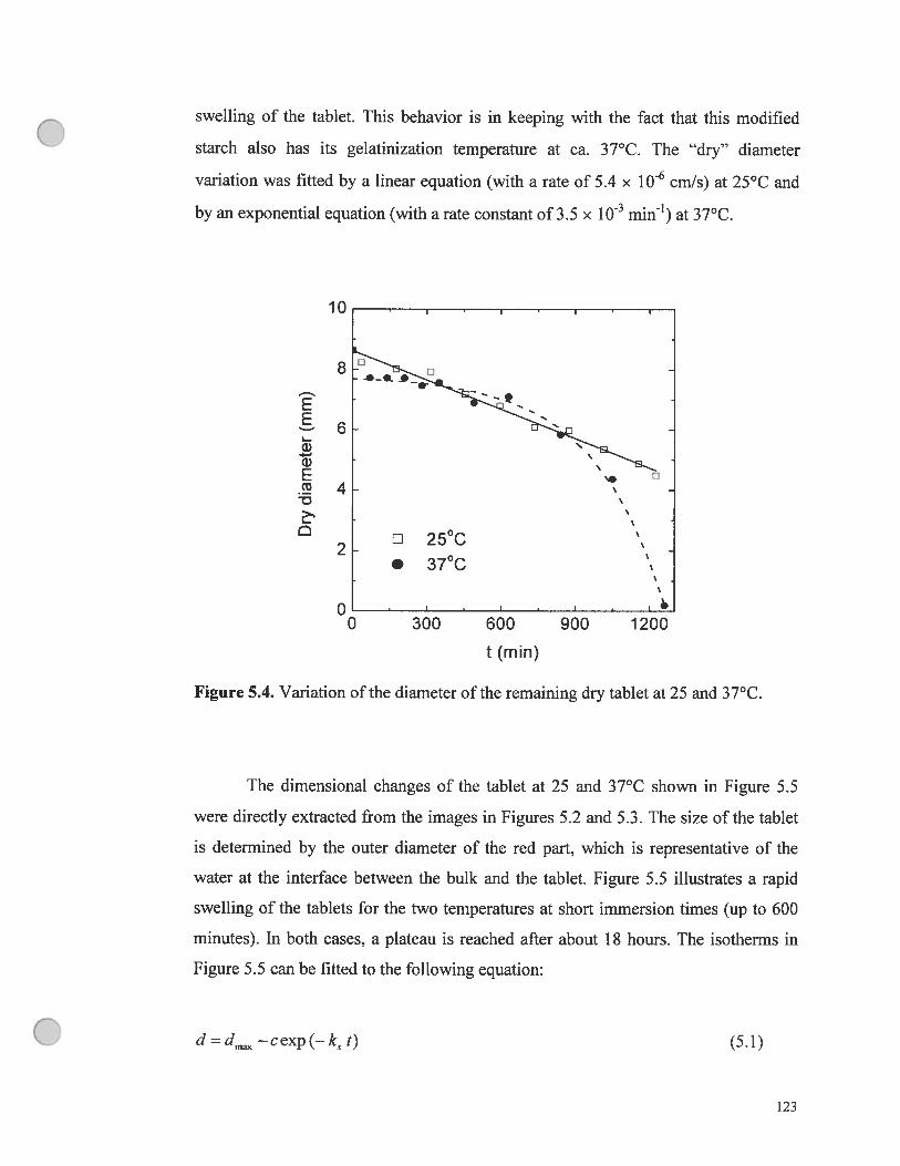
EI.

o4-0E

D

swelÏing of the tablet. This behavior is in keeping with the fact that this modified

starch also has its gelatinization temperature at ca. 37°C. The “dry” diameter

variation was fitted by a linear equation (with a rate of 5.4 x 106 cmls) at 25°C and

by an exponential equation (with a rate constant of 3.5 x i0 min’) at 37°C.

10

8

6

4

2

OO 300

Figure 5.4. Variation ofthe diameter of the remaining dry tablet at 25 and 3 7°C.

The dimensional changes of the tablet at 25 and 37°C shown in figure 5.5

were directly extracted from the images in figures 5.2 and 5.3. The size of the tablet

is determined by the outer diameter of the red part, which is representative of the

water at the interface between the bulk and the tablet. figure 5.5 illustrates a rapid

swelling of the tablets for the two temperatures at short immersion times (up to 600

minutes). In both cases, a plateau is reached afier about 1$ hours. The isotherms in

figure 5.5 can be fitted to the following equation:

d = û’max — cexp t— k, t) (5.1)

600 900 1200

t (mm)

123

where d represents the diameter of the swollen tablet, dmax the maximum diameter of

the swollen tablet at equilibrium, e a constant, t the immersion time, and k the rate

constant of the swelling. Ihe resulting fits show a good agreement with the

experimental data.

13 I I

12. .

11 /

10

• 37°C

8 I

0 400 800 1200 1600

t (mm)

Figure 5.5. Swelling of high amylose starch tablet as a function of time at 25 and

37°C.

The values of dmax and k obtained from the fitting procedure are listed in Table 5.1. It

is interesting to note that the values of dm and k at 37°C are higher than those at

25°C. The swelling of the tablet is more extensive at 37°C, corresponding to an

increase of 34% of tablet diameter, while the increase is only 21% at 25°C. The

resuits obtained for k values indicate that the swelling rate is faster at 37°C than at

25°C. An activation energy of swelling of 38.5 kJ/mol can be roughly estimated from

k values at the two temperatures with the Arrhenius equation. It seems that the value

obtained is realistic. It could be in part a resuit of the breakup of hydrogen bonds,

124

which involves an activation energy in the range of 20 - 40 kJ/mol. The swelling

process is unlike a reaction since the activation energy of reactions occurring in hours

is in the range of 50 - 100 kJ!mol.

From the resuits in figures 5.4 and 5.5, more information of the diffusion

phenomenon can be extracted. Figure 5.6 shows the advancing of the solvent front

(r) toward the center of the tablet at 25 and 37°C as a function of immersion time.

The dashed une is fitted to the Frisch equation:

r=Dxta+c (5.2)

where r represents the distance between the extreme limit of the tablet and the “dry”

part (where water concentration is lower than 1/6 of maximum concentration), t the

immersion time and c a constant. D is a constant proportional to the diffusion rate

and represents the diffusion coefficient or velocity for fickian or Case II process,

respectively. The parameter a is representative of the diffusion kinetics and equals

0.5 for Fickian diffusion and 1 for a Case II (non-ficidan) process [24, 25].

Intermediate values of a between 0.5 and 1 indicate anomalous diffusion. These

values of a are applied in the case of diffusion in a plane sheet and must be corrected

for other sample geometry and when the material swells on ingress of solvent [26,

27]. The resuits in figure 5.6 show clearly the difference in the diffusion processes at

the two temperatures. In fact the advancing of the diffusion front is directly

proportional to the immersion time for the tablet at 25°C and the parameter a is

found equal to 0.92, which is characteristic of Case II diffusion for cylindrical

geometry [27]. A velocity of 0.8 x i0 cmls is obtained from the siope. Also Figure

5.6 shows clearly that the diffusion process of water at 37°C does flot follow Case II

kinetics. However, the Frisch equation is rather empirical when the material swells

and effects of the diffusion from the top and bottom of the tablet must be taken into

account. figure 5.5 shows that swelling is small and can be neglected afier an

immersion time of about 400 minutes for the two temperatures. Moreover, transversal

C images (flot shown here) have demonstrated that the diffusion fronts in the axial

125

direction (i.e. from the upper and lower parts of the tablets) are reached afier 900 and

350 minutes at 25 and 3 7°C, respectively and then effects of the diffusion from the

top and bottom ofthe tablet could be ignored until these times.

Table 5.1. Initial tablet diameter (d0), maximum swelling diameter (dmax) and

rate constants of the swelling (kg) of contramid tablets at two different

temperatures.

Temperature d0 dmax ÏCs

(°C) (mm) (mm) (x i0 min’)

25 8.64 10.4$ 3.52

37 $.64 11.57 6.42

6.

n 25°C• 37°C

4.

EE3 .

_n_

2-p

. ——4 —D

I ••

o • I I

0 300 600 900 1200 1500

t (mm)

Figure 5.6. Advance of solvent front expressed as r, the distance of the solvent front

from the edge of the tablet toward the center of the tablet, at 25 and 37°C as a

function of immersion time.

126

1.0

0.8

“1 0.6D

>%

0.4e

0.2

0 5 10 15 20

distance (mm)

0 3 6 9 12 15

distance (mm)

3 6 9 12

distance (mm)

5 10 15 2

distance (mm)

1.0F 350 min.

0.6

0.6

04

02

nn6 9

distance (mm)

Figure 5.7. Spin density profiles of water (water gradient)

obtained at 25 (A-C) and 37°C (D-f) at short immersion times.

extracted from images

Equation (5.2) could be applied between 400 and 900 minutes for the tablet at 25°C,

but flot at 37°C since the contribution ftom diffusion from the top and the bottom of

the tablet could flot be neglected afler an immersion time of 350 minutes. We can

expect that diffusion at 37°C does flot follow Case II process, but more probably

anomalous diffusion. It must be noted that the gelatinization of ContramidTM occurs

at about 3 7°C, which probably influences the kinetic of water diffusion. The

transition from Case II to fickian diffusion (via anomalous diffusion) with increased

temperature was observed by Weisenberg et al. in the case of PMMÀ-methanol

system [28]. These results are coherent since the change of swelling with temperature

was expected.

The concentration gradient of water can be derived from figures 5.2 and 5.3

o 1._.

0.8

1.0

0.8

ni 0.6D

3,

0.4

0.2

0.0

A 35 min.

..

1.0

0.8

0.6

0.4

0.2

0.0

C 875 min.B 455 min.

0.6

0.4

0.2

,&../t1

0 5 10 15 2C

distance (mm)

1_c .

E 210 min.

0_8

0.6

0.4

0.2

nr. ..-

D,‘ 7omin.

o 15 - 0 3 12 15

127

as shown by the profiles in Figure 5.7 for the tablets at 25 and 37°C. These figures

provide a realistic view of the water diffusion process. Clearly visible are the

advancing water concentration gradients in the tablet. At very short times, these

concentration profiles exhibit at 25°C a rather abrupt decrease going from the

swollen regions to the core, which is characteristic of Case II diffusion. Water

concentration profiles have nearly the same shape at 37°C than at 25°C. Diffusion

process follows probably a quasi-Case II kinetic at 37°C. These resuits are in

agreement with the data obtained from the advance of solvent front in figure 5.6.

5.5. Conclusion

Clearly, NMR Imaging is a useful tool to study the slow release behavior of

pharmaceutical tablets such as ContramidTM in an aqueous environment. The

diffusion of water into the tablets and the swelling of the tablet upon absorption of

water can be visualized with NMR imaging. More quantitative data can be obtained

from the images, in particular the kinetics of the diffusion and swelling processes,

than by an optical imaging approach [20]. The water penetration at 25°C is a Case II

diffusion process, as con±irmed by water concentration profiles. The extent of

swelling of the tablets depends on the temperature and reaches a maximum afler

about 10 hours. The NMR imaging technique also shows a steep advancing solvent

front which should be responsible for the slow release characteristics of this

microporous dmg delivery system [29, 30]. The observed difference in swelling

between 25°C and 37°C, as seen by NMR imaging, is likely caused by the

gelatinization temperature of the excipient ContramidTM at about 3 7°C. In both cases

the tablet, whose dry bulk density was about 0.7 g/cc, is converted into a microporous

hydrogel by the swelling process. A recent rheological study of the swollen tablet

shows a sponge-like behavior [31]. Thus the pressed powder particles in the dry

tablet are fused by the swelling into a coarse network. The latter resuits from pseudo

crosslinking of amylose chains as water penetrates the tablet and converts the mostly

non-crystalline ContramidTM into a highly crystalline state dominated by the double

helix “B” crystal polymorph ofamylase [22, 30]. As a result ofthis mechanism the

ContramidTM tablet self assembles in a microporous hydrogel with limited swelling

12$

o [30].


The authors acknowledge the Natural Sciences and Engineering Research

Council (N$ERC) of Canada for their financial support. R.H.M. is gratehil for the

financial support from Labopharm Inc. and a strategic grant from NSERC.


[1] Fyfe, C. A.; Blazek-welsh, A. 1.1 Control. Release 2000, 68, 313.

[2] Harding, S.; Baumann, H.; Gren, T.; Seo, A. I Control. Release 2000, 66,

81.

[3] Gao, P.; Meury, R. H. I Pharm. Sci. 1996, 85, 725.

[4] Cutts, L. S.; Hibberd, S.; Adier, J.; Melia, C. D. I Control. Release 1996,

42, 115.

[5] Colombo, P.; Bettini, R.; Massino, G.; Catellani, P. L.; Santi, P.; Peppas, N.

A. I Pharrn. Sel. 1995, 85, 991.

[6] Thomas, N. L.; Windle, A. H. Polymer 1978, 19, 255.

[7] Wan, L. S. C.; Prased. K. P. P. DrugDev. md. Pharm. 1990, 16, 921.

[8] Lee, P. I. Pharm. Res. 1993, 10, 980.

[9] Miils, P. J.; Palmstrøm, C. J.; Kramer, E. J. I Mater. Sel. 1986, 2], 1479.

[10] Li, D.; Zhu, S.; Hamielec, A. E. Polymer 1993, 34, 1383.

[11] Weisenberg, L. A.; Koenig, J. L. Macromolecules 1990, 23, 2445.

[12] Grinsted, R. A.; Clark, L.; Koenig, J. L. Macromolecules 1992, 25, 1235

[13] Grinsted, R. A.; Koenig, J. L. Macromolecules 1992, 25, 1229.

[14] Rajabi-Siahboomi, A. R.; Bowtell, R. W.; Mansfield, P.; Henderson, A.;

Davies, M. C.; Melia, C. D. I Pharm. Sel. 1995, 84, 1072.

[15] Rothwell, W. P.; Holecek, D. K.; Kershaw, J. A. I Poiym. Sel., Polym. Lett.

Ed 1984, 22, 241.

129

[16] Rajabi-Siahboomi, A. R.; Bowtell, R. W.; Mansfield, P.; Henderson, A.;

Davies, M. C.; Melia, C. D. Pharm. Res. 1996, 13, 376.

[17] Ghi, P. Y.; Hill, D. J. T.; Whittaker, A. K. Biomacromolecules 2001, 2, 504.

[1$] Koenig, J. L. $pectroscopy ofpolymers; 2nd ed. New York : Elsevier, 1999.

[191 Mateescu, M. A.; Lenaerts, V.; Dumoulin, V. U. S. Patent 5,618,650

[20] Moussa, I. S.; Cartilier, L. H. J Control. Release 1996, 42, 47.

[21] Moussa, I. S.; Lenaerts, V.; Cartilier, L. H. I Control. Release 1998, 52, 63.

[22] Lenaerts, V.; Moussa, I. S.; Dumoulin, L.; Mebsout, F.; Chouinard, F.;

Szabo, P.; Mateescu, M. A.; Cartilier, Louis H.; Marchessault, R. I Control.

Release 1998, 53, 225.

[23] Hyde, T. M.; Gladden, L. f.; Mackley, M. R.; Gao, P. I PoÏym. Sci. Part A,

Polym. Chem. 1995, 33, 1795.

[24] Crank, J.; Park, G. S., in Dffusion in Polymers 1st ed., Academic Press, New

York 1968.

[25] Crank, J., in The Mathematics ofDjffusion 2nd ed., Clarendon Press, Oxford

1975.

[26] Ritger, P. L.; Peppas N. A. I ControL Release 1987, 5, 23.

[27] Ritger, P. L.; Peppas N. A. I Control. Release 1987, 5, 37.

[2$] Weisenberg, L. A.; Koenig, J. L. Appi. $pectrosc. 1989, 43, 1117.

[29] Le Bail, P.; Morin, F. G.; Marchessault. R. H. International Journal of

Biological Macromolecules 1999, 26, 193.

[30] Shifian, D.; Ravenelle, F.; Mateescu, M. A.; Marchessault, R. H.

StarcWStarke 2000, 52, 186.

[31] Ravenelle, F.; Marchessault, R.H.; Légaré, A; Buschmann, M.D. Carbohyd

Polym. 2001, in press.

o130

Chapitre 6

NMR Imaging of High Amylose Starch Tablets:

2. Effect of Tablet Size

C. Malveau, W. E. Baille, X. X. Zhu, R. H. Marchessault

Biomacromolecules 2002, 3, 1249-1254

o

6.1. Abstract

Carbohydrate polymers are widely used for pharmaceutical applications such

as the controlled release of drugs. The swelling and water mobility in high-amylose

starch tablets are important parameters to be determined for these applications. They

have been studied at different time intervals by nuclear magnetic resonance imaging

(NMRI) afier the immersion of the samples in water. These tablets have a hydrophilic

matrix, which swells anisotropically and forms a hydrogel in water. NMRI shows

clearly the anisotropy of the water penetration and the swelling along the radial and

axial dimensions ofthe tablets. Empirical relationships are established to describe the

kinetics of water penetration and swelling of the tablets. Resuits show that water

uptake and tablet swelling strongly depend on the size of the tablets. Gravimetric

measurements of water uptake were also performed in comparison with the NMRI

resuits.

o132

6.2. Introduction

Nuclear magnetic resonance imaging is now ftequently used to study swelling

and water diffusion in hydrophilic tablets [1-11]. Because of its noninvasive and

nondestructive nature, it is a perfect tool to follow the evolution of the tablet’ s shape

and the concentration changes due to solvent uptake. In comparison with other

techniques such as optical methods [12-17) and Rutherford backscattering

spectrometry [1$], NMRI allows the observation of the interior of an object under

investigation without experimental interruption, physical siicing, or other

manipulations. The technique can be easily used to monitor simultaneously different

parts of interest in the object and qualitative/quantitative results can be obtained.

When exposed to water, hydrophilic tablets (e.g. derivatives of cellulose such as

hydroxypropylmethylcellulose [2-7]) form a gel around the tablet, which, within a

certain time limit, physically restricts the dissolution and diffusion of drugs and

provides a mechanism for controlled release. The understanding ofthese processes is

important in the formulation of a controlled release system to achieve the maximum

pharmacological effectiveness [2].

Amylose is a linear (1,4)-a-glucan (with a molecular weight of about 500

000) in starch while amylopectin is a higffly branched (1,4)-Œ-glucan (with a

molecular weight of 50-100 million) with multiple short chains arranged in a

racemose fashion. High-amylose starch is a hybrid containing typically 70% amylose

and 30% amylopectin. The cross-linked high amylose starch used has advantages in

drug delivery such as the absence of erosion and limited swelling [19]. A unique

mechanism which controls swelling in this system is the transformation of amylose

from the V-type single helix polymorph to the B-type double helixes during water

uptake [19, 201. Contraiy to other polymer matrixes, an increase in the degree of

chemical cross-linking leads to an increase in water uptake as well as in the drug

release rate [21-24]. The rheological behavior ofthe swollen tablet is spongelike [25].

Thus, the pressed spray-dried particles in the dry tablet are fused during the water

uptake with subsequent helix rearrangement into a porous hydrogel.

In our first report [11], we have studied the effects of temperature on tablet

swelling and water uptake and found that the water penetration at 25 oc is a case iI

133

diffusion process. The extent of swelling of the tablets depends on the temperature

and reaches a maximum afler an immersion time of about 10 h. The NMR imaging

technique has also shown a steep advancing solvent front which should 5e

responsible for the slow release characteristics of this microporous drug delivery

system [20, 26]. The observed difference in swelling between 25 and 37 oc is caused

by the different degrees of transformation from V- to B-type of this modified starch

excipient. However, the tablet size is an important parameter in the slow release

process because of the importance of anisotropic diffusion and swelling. The goal of

this study is to understand the diffusion phenomena as related to the properties of the

high-amylose starch. In this paper, we report the NMR images of the water uptake

and swelling of high-amylose starch tablets of different sizes at 37 °c and the

interpretation of the kinetic results from the anisotropic swelling process. Gravimetric

measurements of water uptake were also carried out.


6.3.1. Tablet Preparation

High-amylose starch tablets were supplied by Labopharm Inc., prepared from

Hylon VII purchased from National Starch co. The excipient used is pretreated

according to the following patented procedure [27]: high-amylose starch granules

were gelatinized (irreversible phase transition) in 4% aqueous NaOH and then cross

linked with epichiorohydrin in the highly swollen state. The washed and spray-dried

product has the trade name contrmiid. The spray-dried contramid powder was used

for the preparation of the tablets by using a single station tablet press (Stokes model

$4).

Two samples were studied (Table 6.1). The first one (Contramid-I) was

prepared with a compression force of 10.6 kN, leading to a hardness (the peak force

needed to break the tablet) of 19$ N. The second one (contramid-II) is smaller in

size and was prepared with the same compression force to yield a hardness of 69 N.

6.3.2. NMR Imaging Experiments

The ‘H NMR imaging experiments were performed at a ftequency of 300

MHz (7 T) using a Bruker DSX-300 NMR spectrometer equipped with a

C microimaging probe, which can accommodate a maximum sample size of 20 in

134

diameter. The system is also equipped with three orthogonal field gradient cous

permitting a maximum gradient of 100 G/cm. Tablets were placed on a support,

which allowed tbree-dimensional water penetration (Figure 6.1), inside a 15-mm o.d.

NMR tube containing a mixture of H20 and D20 (50:50). The H20/D20 mixture was

chosen in order to increase the 1H T1 ofwater thereby enabling a better discrimination

between water inside and outside the tablet. Moreover this allowed the use of the

deuterium lock, which helped to prevent the drifting of the magnetic field. A standard

siice-selective spin-echo imaging sequence (Figure 6.2) was used to acquire images

of the water inside the amylose tablet. A suce of 500-tm thickness was selected

parallel to the main magnetic field (axial axis) by the use of a sinc-shaped selective

pulse and a giadient of 12 G/cm. four scans were accumulated to obtain a 256 x 256

pixel image, leading to an in-plane nominal resolution of 78 p.m. An echo time (TE)

of 4 ms and a repetition time (TR) of 2 s were fixed leading to an experimental time

of about 35 min for each image. Ail experiments were performed at 37 oc.

support made of Teflon

H20 + D20

Figure 6.1. Schematic diagram of the tablet arrangement for the NMRI experiment.

135

Table 6.1. Physical characteristics of the tablets.

Weight Diameter Thickness Hardness Surface Volume SN DensityContramid(mg) (mm) (mm) (N) (mm2) (mm) (mm’) (mg/mm3)

I 200 8.6 2.7 197.8 191 159 1.2 1.3

11 23.5 4.8 1.2 69 54 22 2.5 1.1

Gr

->Tt /2

H

Figure 6.2. The spin-echo pulse sequence used to acquire two-dimensional NMR

image. TR and TE are the recovery time and the echo time, respectively. G, G and

G represent the slice, phase and read gradients, respectively.

6.3.3. Measurement of Water Uptake

A gravimetric method was used to record water uptake of Contramid-I and -

II. At appropriate time intervals, each tablet was removed from water and weighed

afier removing water adhering to the outer surface of the tablets with a paper towel.

it /2

TR

Tt echo

RF

G

TE

n n

136

Q6.4. Resuits and Discussion

Figure 6.3 shows the time dependence of the two-dimensional proton NMR

images of an axial suce through the center of the Contramid-I tablet. Water

penetration is followed by the recession of the dark blue part in the middle of the

images, which represents the dry portion of the tablet. The two dark blue rectangular

shapes at the bottom of each image correspond to the Teflon support (see Figure 6.1).

f igure 6.3 exhibits the swelling process of the tablet, which is represented by the red

contour at the extreme limits of the tablet. This red area corresponds to the water

inside the saturated gel surface. This saturated gel is the result of a series of processes

starting with water penetration, which provokes a conformation change of the

polymers. Initially, the dry starch is arranged mainly in the V-type single lieux form

[19, 26].

19.2h 25.lh 32.Ïh 41.4h

Figure 6.3. NMR images showing the water penetration into Contramid-I tablet at 37

°C at different times. Each image is the sum of 4 accumulations with a repetition time

of 2 s, yielding an experimental time of 35 min. The nominal spatial resolution in

plane is 78 im, with a suce thickness of 500 jim.

When immersed in water, it partly converts to the B-type hydrated double lieux

conformation, forming a three-dimensional network [19, 20]. As a resuit, the

0.6 h 2.9 h 7.6 h 12.2 h

137

Contramid tablet self-assembles into a microporous hydrogel with limited swelling

[20]. The apparent higher water concentration near the gel surface compared to

outside the tablet is the resuli of attenuation of the signal of free water due to a

relaxation effect. The signal intensity in a spin-echo experiment can be described by

t TRi TE8=kp 1—exp(——) exp(——--) (6.1)

L

where k is a proportionality constant, p the spin density, TR the repetition time, TE

the echo time (see Figure 6.2), and T1 and T2 are the longitudinal and the transversal

relaxation times, respectively. T1 of ftee water is about 4 s and the recovery time TR

was fixed at 2 s. Therefore, the bulk water magnetization cannot retum completely to

equilibrium (39% as calculated from eq 6.1), while the magnetization of water inside

the tablet can do much better (ca. 93%) since it has a shorter T1 of about 750 ms

(value obtained when the water concentration inside the tablet reaches the highest).

Since the relaxation times of water inside the tablet decrease with decreasing water

content, no further attenuation of signal intensity should be caused by longitudinal

relaxation. This resuits in an apparent higher intensity of the water signal inside the

gel in comparison to the bulk water. On the other hand, the effect of TE (4 ms, a

minimum value that seems to allow a good execution of the imaging experiment)

should flot have an attenuation effect on the NMR signal of the bulk water, wbile it

has a larger effect on the signal of water inside the tablet since it has a shorter T2 (ca.

25 ms at the maximum water concentration of the final stage). In any case, this

intensity difference of water inside and outside the tablet allows us to follow more

easily the swelling of the tablet with time. Also, Figure 6.3 shows clearly that water

diffusion is a symmetric process and equilibrium is reached after about 41 h.

The same experiments were performed on the smaller Contramid-II tablet.

Some differences were observed. As expected, the equilibrium was reached faster for

the tablet of a srnaller size. No further changes were obseiwed afier an immersion

time of about 17 h (as in the case of Contramid-I afier 41 h). However, we have

138

observed a difference between the tablet center and the outer part, i.e.. the water

content is slightly lower in the middle of the tablet than in the gel layer. This may be

a resuit of the rapid water uptake of this small tablet at the beginning, which in tum

caused a rapid swelling of the outer part of the tablet. When the swelling is fast,

amylose does flot undergo completely the transformation from V- to B-type. When

the water penetration is siower, as observed for the inside of the small tablet or for

Contramid-I, the transformation from V- to B-type occurs more easily. Previous

works by Moussa et al. and Shifian et al. have shown a higher degree of chemical

cross-linking led to a more significant swelling of the tablet and a lower degree of

transformation of amylose to the B-type [20, 24]. Amylose in the inner part has a

higher proportion of B-type double helix conformation and thus swells less, which

leads to a slightly lower water concentration.

The dimensional changes (% swelling, defined as the increase in dimension as

a percentage of the initial tablet size) of the high-amylose starch tablets are shown in

Figure 6.4. They are directly extracted from images (with the help of the red contour,

which corresponds to the water inside the saturated gel layer and is representative of

the interface between the tablet and the solvent). At the beginning ofthe immersion, a

fast swelling of the two tabiets along the two directions is observed (less than 3 h and

12 h for Contramid-II and Contramid-I, respectively), followed by a small increase of

the tablet size. No dimensional changes are observed afier 5 and 1$ h for the 2

tablets, respectively. However, aller this period, water continues to penetrate

insidethe tablet, as observed by the increase of the signal intensity inside the tablet

for longer immersion time (see figure 6.3 for Contramid-I). $ince the water

concentration in the saturated gel layer remains constant, the increase in water

concentration within the tablet is due to the penetration of water from the buïk

solvent by an osmotic effect. The change of intensity inside the tablet aller the end of

the swelling cannot be the result of a relaxation effect. In fact, relaxation time maps

at equilibrium have shown that T1 and T2 have a nearly uniform value ah over the

tablet (T1 750 ms, T2 25 ms). This resuit indicates that water concentration is

homogeneous ail over the tablet and the total quantity of water in the thin suce (500

tm) under investigation continues to increase even aller the end of the dimensional

139

swelling. This may be caused by several factors. First, the graduai transformation of

amylose from V- to B-type limits the swelling of the tablet; second, this coincides

with the weight drop of the wet tablet (Figure 6.6), indicating the beginning of the

dissolution of the tablet at the outer surface; and third, the inner part of the sample

corresponds to only a very small portion of the whole sample and its effect on the

total volume is flot significant. For each sample, the swelling along the axial

dimension is more pronounced than that along the radial dimension. Ibis is

particularly visible for Contramid-1I. Ibis difference can be explained by the fact that

the compression force is applied along the axial direction, giving a disk-like shape to

the smalt dry particles in the tablet, wbich tend to regain spherical symmetry in water.

However, the Contramid-II tablet is subject to a larger swelling, leading to an

increase of nearly 200% in thickness and 50% in diameter. In the case of Contramid

1, the increase is limited to 60% in thickness and to nearly 40% in diameter. Although

the fabrication compression force was almost identical for the two tablets. the smaller

sample has a much lower hardness so that it is easier to swell. For Contramid-I at 25

°C, we have found a lower swelling increase of 20% along the radial direction [111.

To quantify these differences, tablet swelling data were fitted to ifie following

equation with good agreements between experimental and fitted values:

Ï = — e exp (—kt) (6.2)

where l and 1max represent the dimensions (diameter or thickness) of the swollen

tablet after an immersion time t and at equilibrium, respectively, e is a pre

exponential constant, and k is a rate constant. The values of k and ‘max are listed in

Table 6.2. The resuits are consistent with our previous study on Contramid-I for

which we found a swelling in diameter of 34% with a rate constant of 0.39 h’ [11].

As expected, the rate constant is higher for the smaller tablet. One reason is that the

surface/volume ratio for the smaller tablet is twice as much as for the bigger one.

This implies that the penetration of water is easier for Contramid-II than for

Contramid-I. Moreover, the rate is higher along the axial direction than along the

140

o

c,)C

U)

U)

Time (h)

Figure 6.4. Swelling in both axial (O) and radial (.) directions

and Contramid-II (B) tablets. Solid unes show fits ofthe data to eq 6.2.

of Contramid-I (A)

80

radial direction for the smaller tablet. No difference of rate constants was observed

between the two directions for Contramid-I.

60

40

20

o

250

200

c,)C

U)

0 10 20 30 40 50

lime (h)

150

100

50

OO 5 10 15

141

Table 6.2. Parameters obtained by fitting the tablet swelling

data in figure 6.4 to eq 6.2.

in diameter in thicknessContramid

k (lï’) ‘max (%) k (lï’) ‘max (%)

I 0.3 34.9 0.3 57.9

II 0.9 47.7 1.1 180.9

This can 5e explained by the very fast increase in the thickness observed at very short

time. This increase was flot taken into account in our fitting.

Figure 6.5 shows the evolution of the dimension of the dry part of the tablet

as a function of immersion time for both Contramid-I and II. The dimension of the

dry part is defined as the size of the tablet (along the radial or the axial axis) where

the water concentration is lower than 1/6 of the maximal concentration of water

inside the gel layer. for the two samples, we can observe the same trend for each

axis. As shown in Figure 6.5A, the diameter of the dry part of the tablet decreased

only slightly during a relatively long initial period (about 7 h for the small tablet and

10 h for the large one) and then decreased more drastically. On the other hand, the

decrease of dry thickness is linear as a function of time for both samples (figure

6.5B). The difference in the radial and axial directions ofthe tablets should be related

to the swelling process of the tablets. In figure 6.4, it is clear that the degree of

swelling in the axial direction is much greater than in the radial direction. In the first

hours of immersion, water was consumed for the swelling of the sample in the axial

direction and thus the dry diameter was not affected very much. This shows that

water penetration occurred mainly along the axial direction, due mainly to capillary

actions. Thus the dry thickness decreases continuously while the dry diameter

remains nearly constant in this period.

In our previous paper [1 1], we have shown that the decrease in the dry

diameter of Contramid-I at 25 oc was linear as a function of immersion time. The

temperature difference in the two cases should 5e noted.

142

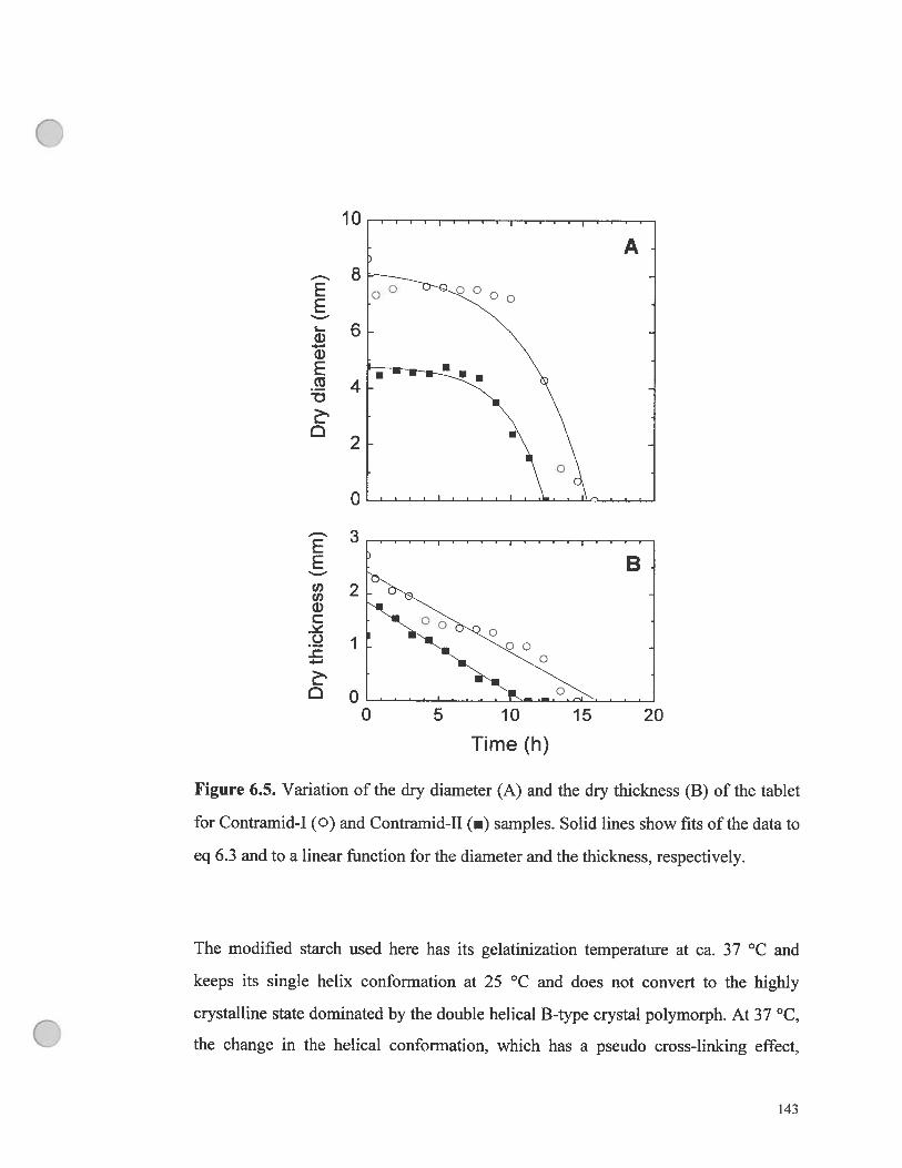
figure 6.5. Variation of the dry diameter (A) and the dry thickness (B) of the tablet

for Contramid-I (o) and Contramid-II (.) samples. Solid unes show lits ofthe data to

eq 6.3 and to a linear function for the diameter and the thickness, respectively.

The modified starch used here has its gelatinization temperature at ca. 37 oc and

keeps its single helix conformation at 25 °c and does flot convert to the highly

crystalline state dominated by the double helical B-type crystal polymorph. At 37 oc,

the change in the helical conformation, which has a pseudo cross-Iinking effect,

10

Eg‘—6Q)

4-,

G)E.s 4

2

2

O

gU)U)G)

o-

4-,

D

1

OO 5 10 15 20

Time (h)

143

proceeds rapidly and this change in conformation affects the swelling behavior of the

polymer [20]. Therefore, the resuits obtained at the two temperatures cannot be

directly compared.

For the decrease in the dry diameter, the trend can be fitted to an exponential

function as shown below:

dd =d0 —cexp[ku (t—tv)] (6.3)

where dd represents the diameter of the dry part of the tablet, d0 the initial tablet

diameter, c a pre-exponential constant, lcd a rate constant, t the irmnersion time, and tf

the immersion time when dd equals 0. On the other hand, a linear function can be

used to describe the decrease in the dry thickness of the tablets. The fitting

parameters to these functions are listed in Table 6.3. The fits are representative ofthe

difference along the two directions perpendicular to each other. For the dry diameter,

the rate constant for the small tablet is about 70% higher than for the large tablet (0.4

h1 versus 0.24 h’). But the difference of swelling rates is smaller along the axial

direction.

Table 6.3. Parameters obtained by fitting the data in figure 6.5 to eq 6.3

for the dry diameter and to a linear function for the dry thickness.

in diameter in thicknessContramid

t (h) d0 (mm) lcd (h’) d0 (mm) r (mmlh)

I 15.8 8.3 0.24 2.4 0.15

II 12.4 4.8 0.40 1.8 0.17

We already know that the dry diameter decrease with a rate of 0.19 mm!h for the

Contramid-I at 25 °C, whereas we have obtained a rate constant of 0.21 h’ at 37°c.”

144

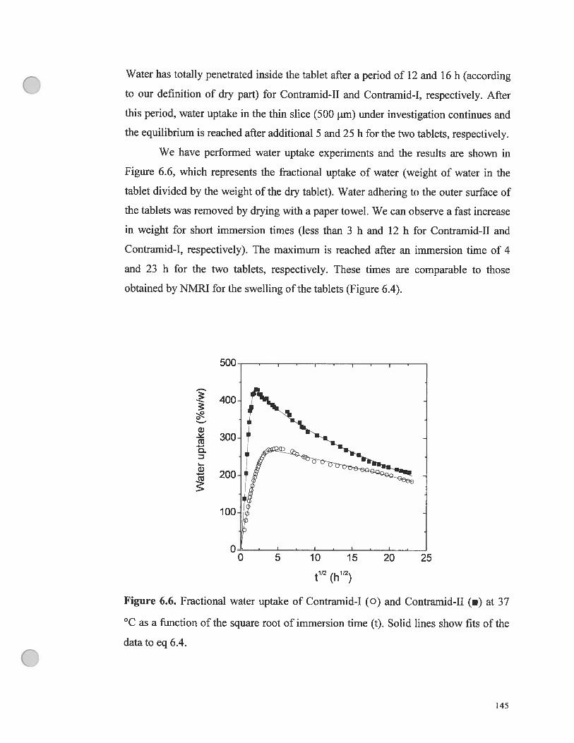
Water has totally penetrated inside the tablet afier a period of 12 and 16 h (according

to our definition of dry part) for Contramid-II and Contramid-I, respectively. Afler

this period, water uptake in the thin suce (500 tm) under investigation continues and

the equilibrium is reached afier additional 5 and 25 h for the two tablets, respectively.

We have performed water uptake experiments and the resuits are shown in

figure 6.6, which represents the fractional uptake of water (weight of water in the

tablet divided by the weight of the dry tablet). Water adhering to the outer surface of

the tablets was removed by drying with a paper towel. We can observe a fast increase

in weight for short immersion times (less than 3 h and 12 h for Contramid-II and

Contramid-I, respectively). The maximum is reached after an immersion time of 4

and 23 h for the two tablets, respectively. These times are comparable to those

obtained by NMRI for the swelling ofthe tablets (figure 6.4).

G)

.1-i

Q-D

G)

Figure 6.6. fractional water uptake of Contramid-I (O) and Contramid-II (.) at 37

°C as a function of the square root of immersion time (t). Solid unes show fits of the

data to eq 6.4.

0 5 10 15 20 25

t112 (h’)

145

Then the disintegration (or dissolution) of the tablets plays the main role as illustrated

by the weight decreases of the samples (Figure 6.6). As observed previously by

NMRI for tablet swelling, Contramid-II is subject to a larger water uptake, with a

maximal water uptake of about 43 0%, whereas the maximal is about 270% for

Contramid-I. To quantify the evolution of the ftactional weight uptake. the data were

fitted to the following equation with good agreements:

MHO M2 = max

—cexp(—k t)—kdSSt” (6.4)‘1diy 1diy

where MH2O and Md represent the mass of water inside the tablet afier an immersion

time t and the mass of the dry tablet, respectively, e is a pre-exponential constant, k

and kdjss are rate constants for water uptake and tablet dissolution, respectively, and

is a constant. The fitting parameters are listed in Table 6.4. The experiment was

repeated for the smaller tablet (Contramid-II). We have observed a somewhat lower

water uptake (Mm = 475%) and a smaller dissolution rate constant (kd = 61.3 W’)

but the rate constant for water uptake kw and the constant Œ are identical. As

expected, the rate constant is higher for the smaller tablet. The rate constants for

water uptake obtained are identical to those obtained by NMRI for tablet swelling

(Table 6.2). for the volume change (calculated from data in figure 6.4), a rate

constant of 0.3 and 0.8 h’ was obtained for Contramid-I and II, respectively. The

disintegration ofthe smaller tablet occurs early as illustrated in figure 6.6.

Table 6.4. Parameters obtained by fiftiug the water

uptake data in figure 6.6 to eq 6.4.

Contramid Mmax (%) kw (W’) kdiss (h) a

I 282 0.3 2.7 0.6

II 537 1.1 73.7 0.2

146

6.5. Conclusion

This work shows the usefiilness of the NMR imaging technique in obtaining

information valuable to the development of controlled release systems made from

biomacromolecules. It provides more qualitative and quantitative information on the

nature of the water penetration and swelling processes than optical imaging [24]. We

have observed anisotropic swelling of the high-amylose starch tablets, which arises

from the applied axial compression force during tablet fabrication. Previous work has

shown that the greater the force is, the smaller the wet modulus ofthe swollen tablet

[25]. Water uptake and tablet swelling strongly depend on tablet size. A difference

was observed in the kinetics of water penetration along the two directions. In

particular, the decrease of dry diameter with immersion time is more gradual while

the decrease of the dry thickness is more rapid and shows a linear relationship with

time, probably due to a rapid capillary penetration of water in the axial direction. The

kinetic data of tablet swelling show that the swelling rate is faster for the small tablet

along both swelling directions since the surface/volume ratio is much larger for the

smaller tablet. The gravimetric water uptake measurements confirm the resuits

obtained with NMRI, which is evident by comparing the kinetic data obtained from

figures 6.4 and 6.6.


The authors wish to thank the Natural Sciences and Engineering Research

Council (NSERC) of Canada for their financial support and Bristol Myers Squibb for

their financial aid in acquiring the Paravision Software.


[1] Harding, S.; Baumann, H.; Gren, T.; Seo, A. I Control. Release 2000, 66,

81.

[2] fyfe, C.A.; Blazek-Welsh, A.I. I Control. Release 2000, 68, 313.

[3] fyfe, C.A.; Grondey, H.; Blazek-Welsh, A.I.; Chopra, S.K.; fahie, B.J. I

ControL Release 2000, 68, 73.

[4] Fahie, B.J.; Nangia, A.; Chopra, S.K.; Fyfe, C.A.; Grondey, H.; Blazek, A. I

Control. Release 1998, 51, 179.

147

Q[5] Fyfe, C.A.; Blazek, A. I. Macromolecules 1997, 30, 6230.

[61 Rajabi-$iahboomi, A.R.; Bowtell, R.W.; Mansfield, P.; Davies, M.C.; Melia,

C.D. Pharm. Res. 1996, 13, 376.

[7] Rajabi-Siahboomi, A.R.; Bowtell, R.W.; Mansfield, P.; Henderson, A.;

Davies, M.C.; Melia, C.D. J Control. Release 1994, 3], 121.

[8] Kojima, M.; Ando, S.; Kataoka, K.; Hirota, T.; Aoyagi, K.; Nakagami, H.

Chem. Pharm. Buli. 1998, 46, 324.

[9] Hyde, T.M.; Gladden, L.F.; Payne, R. I Control. Release 1995, 36, 261.

[10] Ashraf, M.; luomo, V.L.; Coffin-Beach, D.; Evans, C.A.; Augburger, L.L.

Pharm. Res. 1994, 11, 733.

[11] Baille, W.E.; Malveau, C.; Zhu, X.X.; Marchessault, R.H.

Biomacromolecules 2002, 3, 214.

[12] Gao, P.; Meury, R. H. J Pharm. Sci. 1996, 85, 725.

[13] Cutts, L. S.; Hibberd, S.; Adier, J.; Melia, C. D. I Controt. Release 1996, 42,

115.

[14] Colombo, P.; Bettini, R.; Massino, G.; Catellani, P. L.; Santi, P.; Peppas, N.

A. I Pharm. Sci. 1995, 85, 991.

[15] Thomas, N. L.; Windle, A. H. Folymer 1978, 19, 255.

[16] Wan, L. S. C.; Prased, K. P. P. DrugDev. IncL Pharm. 1990, 16, 921.

[17] Lee, P. I. Pharm. Res. 1993, 10, 980.

[18] Milis, P. J.; Palmstrøm, C. J.; Kramer, E. J. J Mater. $ci. 1986, 2], 1479.

[19] Lenaerts, V.; Moussa, I.; Dumoulin, Y.; Mebsout, F.; Chouinard, F.; Szabo,

P.; Mateescu, M.A.; Cartilier, L.; Marchessault, R. J Control. Release 1998,

53, 225.

[20] Shifian, D.; Ravenelle, F.; Mateescu, M.A.; Marchessault, R.H.

Starch/Stfirke 2000, 52, 186.

[21] Lenaerts, V.; Dumoulin, Y.; Mateescu, M.A. I Control. Release 1991, 15,

14$

39.

[22] Moussa, I.$.; Cartilier, L.H. Proc. ]st World MeetingAPGl/APV 1995, 241.

[23] Moussa, I.S.; Lanaerts, V.; Cartilier, L.H. I Control. Release 1998, 52, 63.

[24] Moussa, I.S.; Cartilier. L.H. I ControL Release 1996, 42, 47.

[25] Ravanelle, F.; Marchessault, R.; Légaré, A.; Buschmann, M.D.; Carbohyd

Polym. 2001, 47, 259.

[26] Le Bail, P.; Morin, f. G.; Marchessault, R. N. Int. I Biol. Macromol. 1999,

26, 193.

[27] Mateescu, M.A.; Lenaerts, V.; Dumoulin, V. U.S. Patent 5,618,650.

o149

Conclusion générale

Nous vous avons présenté un certain nombre d’études sur le processus de la

diffusion dans les systèmes polymères selon deux approches complémentaires. Dans

la première approche, plusieurs techniques de résonance magnétique nucléaire à

gradient de champ pulsé (RMN PFG) ont été utilisées pour mettre en évidence

l’influence de certains paramètres physico-chimiques peu étudiés mais qui peuvent

s’avérer très déterminants pour la diffusion. Nous avons étudié l’influence de la

forme du diffusant, de même que celle des interactions chimiques entre le diffusant et

la matrice polymère (les interactions non-hydrodynamiques) sur le processus de

diffusion. Les résultats expérimentaux ont généralement été utilisés afin de vérifier

les limites d’applicabilité du modèle théorique de Petit et al. par rapport à l’effet de la

forme du diffusant et tes interactions entre le diffusant et le polymère. Pour les études

sur l’influence des interactions, le modèle de Phillies a été utilisé pour l’analyse des

résultats expérimentaux. Dans la seconde partie, nous avons étudié et démontré par

l’imagerie RMN les facteurs influençant la diffusion de l’eau dans des comprimés

d’amidon à haute teneur en amylose. Nous avons aussi étudié les facteurs affectant le

processus de gonflement de ces comprimés. Les résultats expérimentaux obtenus

dans cette partie ont été analysés par diverses équations analytiques empruntées à la

littérature.

7.1. L’étude de la diffusion par R1vIN PFG

Pour l’étude de l’effet de la forme du diffusant sur le processus de la diffusion

dans les systèmes polymères, les diffusants retenus sont des polymères linéaires,

hyperbranchés et dendritiques. Cependant, pour mieux comprendre et mieux illustrer

cet effet de la forme, nous avons entrepris d’étudier les effets d’autres paramètres tels

que la masse molaire du diffusant, la concentration en polymère, la température. En

ce qui concerne l’influence des interactions chimiques, elle a été démontrée en

utilisant des petites molécules contenant des groupes fonctionnels (par exemple de

l’acide acétique et de l’éthylène glycol avec ou sans groupement alkyl terminal) et

des matrices polymères possédant aussi des groupes fonctionnels.

150

7.1.1. L’effet de la masse molaire du diffusant

Il a été démontré qu’en absence de la dominance des effets de la forme et des

interactions, le coefficient d’auto diffusion des diffusants dans le solvant (D0)

diminue grandement avec l’augmentation de la masse molaire. Nous avons observé le

même effet aussi bien pour les diffusants polymères que pour les diffusants de petites

tailles. Cette observation n’a rien de particulière car plusieurs travaux proposés dans

la littérature ont fait état de cet effet [l-10]. Cette diminution de D0 avec la masse

molaire est obtenue lorsque le processus de la diffusion est principalement contrôlé

par la masse molaire du diffusant. De plus, il est démontré par l’équation de Stokes

Einstein que le coefficient de diffusion est inversement proportionnel au rayon

hydrodynamique de la molécule diffusante. Il est aussi démontré que le rayon

hydrodynamique varie proportionnellement avec la masse molaire de la molécule

diffusante à la puissance 1/3 dans le cas d’une molécule sphérique et à la puissance

1/2 dans le cas d’une molécule cylindrique [11, 12]. De ce fait, en absence d’effets

dus aux interactions dans le milieu et lorsque les diffusants ont la même forme, la

diffusion doit normalement diminuer avec l’augmentation de la masse molaire du

diffusant. Cette diminution peut être expliquée en se basant sur la théorie du volume

libre. Cette dernière décrit le processus de la diffusion d’une molécule donnée

comme étant tributaire de la probabilité de la formation d’un volume critique adjacent

suffisamment grand pour permettre à une molécule de taille inférieure à ce volume

critique de faire le saut de sa position initiale vers ce volume [13]. Comme la

probabilité de la formation d’un plus grand volume critique est inférieure à celui d’un

plus petit volume, il en résulte une diffusion plus lente avec l’augmentation de la

masse molaire. En d’autres mots, cette molécule aura besoin d’une plus grande

énergie pour passer d’un environnement à un autre.

7.1.2. L’effet de la concentration en polymère

L’effet de la concentration en polymère sur le processus de diffusion a été au

coeur de toutes les mesures effectuées dans la première partie de cette thèse. Nous

avons démontré que l’augmentation de la concentration en polymère conduit à une

diminution régulière et non-linéaire du coefficient d’auto-diffusion. Malgré que les

concentrations en polymère utilisées (de 0.03 à 0.38 g!mL) couvrent toute la gamme

151

de concentrations qui inclut le régime dilué, le régime semi-dilué et le régime

concentré, nous n’avons pas observé de changement important dans la valeur de D

avec les changements de régimes. Ces résultats sont en accord avec les données de la

littérature concernant des diffusants de taille similaire [1-101. Cependant, il est connu

que certaines propriétés des solutions de polymères (par exemple la viscosité)

changent grandement lorsqu’on passe d’un régime dilué à un régime semi-dilué [14,

15]. La remarque que l’on peut faire sur ces résultats est que le processus de diffusion

n’est pas suffisamment sensible aux changements de régimes. Cependant, on peut se

demander si cette insensibilité au changement de régime n’est pas reliée à la faible

taille des diffusants car il a été démontré que la masse molaire du polymère

influençait le processus de diffusion uniquement lorsque la taille du diffusant est

supérieure à une certaine valeur [16, 17]. Néanmoins, nous avons expliqué cette

diminution du coefficient d’auto-diffusion en regardant les solutions polymères avant

et après la concentration critique de recouvrement (c*). Avant c, la diffusion est

influencée par la viscosité de la solution. Cependant, après c, on doit également

considérer l’influence de la formation d’un réseau entre les chaînes de polymères

(l’enchevêtrement) sur le processus de diffusion.

7.1.3. L’effet de la température

Nous avons observé une augmentation du coefficient d’auto diffusion avec la

température. De manière générale, cette augmentation du coefficient d’auto diffusion

s’explique par le fait qu’en augmentant la température, la molécule diffusante

acquiert une plus grande mobilité, ce qui indique qu’il y a moins d’interactions entre

le diffusant et son environnement et une plus faible viscosité de la solution. Cette

augmentation de la mobilité explique pourquoi nous avons observé une augmentation

plus significative de D avec la température lorsqu’on est dans un régime dilué. Elle

permet aussi de comprendre l’effet plus significatif de la température sur le

coefficient d’auto diffusion des diffusants de plus faibles masses molaires. La

détermination de l’énergie d’activation apparente en fonction de la concentration en

polymère confirme ces observations et les valeurs obtenues varient entre 16 et 45

kJ/mol pour tous les diffusants utilisés. Cette énergie apparente augmente avec la

masse molaire, la magnitude des interactions et la concentration en polymère.

152

7.1.4. L’effet de la forme du diffusant

Grâce aux études comparatives effectuées entre des diffusants polymères

(polymères linéaires, hyperbranchés et dendritiques), nous avons constaté que pour

une masse molaire similaire, le coefficient d’auto diffusion diminue en partant du

diffusant dendritique au diffusant linéaire (dendritique > hyperbranché > linéaire). Le

même résultat est obtenu pour toute la gamme de concentrations en polymère utilisée

dans cet ouvrage. En se basant sur l’absence d’interaction entre ces diffusants et la

matrice polymère (PVA), de même que sur leur différence de la distribution de

densité, nous avons attribué cette diminution de D entre ces diffusants (dendrimère,

hyperbranché, linéaire) à leur forme respective. Il faut noter que la valeur de cette

distribution de densité est qualitative. Néanmoins, ce paramètre est utilisé dans de

nombreuses études pour caractériser l’arrangement d’une chaîne de polymère en

solution [1 8-28). Par exemple, une valeur de l’exposant de flory (Œ) de 0.33 indique

que la distribution de densité est uniforme alors qu’une valeur de 0.5 indique une

distribution fractale. Cependant, une question demeure: quelle est la forme exacte de

chaque diffusant?

Ces résultats démontrent clairement que la forme de la molécule diffusante a

un effet non négligeable sur le processus de la diffusion. Bien que l’influence de la

forme du diffusant soit significative, on constate peu d’étude a été fait sur le sujet

[29, 30]. Actuellement, aucun des modèles théoriques de diffusion ne tient en compte

de cet effet de la forme [3 1-33]. Nous savons que dans un système binaire (soluté

solvant), l’équation de Stokes-Einstein peut être adaptée selon la forme du diffusant

[12]. Il serait important d’inclure aussi cet effet dans les modèles théoriques actuels.

7.1.5. L’effet des interactions diffusan-polymère

Les interactions spécifiques, telles que les ponts hydrogène qui jouent un rôle

très important dans le processus de diffusion. Ces interactions sont connues pour

retarder considérablement le processus de diffusion [34]. En effet, Nous avons

observé qu’en présence de ponts hydrogène entre le diffusant et le polymère, le

coefficient d’auto-diffusion ne variait plus en fonction de la masse molaire. En ce

sens, nous avons obtenu des valeurs de coefficients d’auto-diffusion plus faibles pour

l’éthylène glycol, le diéthylène glycol et le triéthylène glycol par rapport à leurs

153

dérivés contenant un ou deux groupes terminaux d’éther de méthyle. De plus, cet

écart s’accentue avec la concentration en polymère. Cependant, la normalisation de

ces coefficients d’auto-diffusion (D/D0) a permis de mieux faire ressortir cet effet et

aussi de dire clairement que les interactions diffusant-polymère observées ne sont pas

des interactions hydrodynamiques. Nous avons observé que le coefficient d’auto-

diffusion varier grandement en fonction des groupes fonctionnels sur le diffusant

(acide carboxylique, amine, hydroxyle). Le même effet est également obtenu en

fonction des matrices de polymères ayant aussi des groupements latéraux d’acide

carboxylique, d’amine, d’amide et d’hydroxyle montrent également l’effet des ponts

hydrogène sur la diffusion. Ces résultats nous ont permis de constater que la

magnitude de l’effet des ponts hydrogène dépend des groupes fonctionnels.

Cependant, le mécanisme par lequel les groupes fonctionnels retardent le processus

de la diffusion ne nous paraît pas évident pour l’instant. En ce sens, des études

futures devraient être faites pour élucider ce mécanisme.

7.1.6. Le modèle de Petit et al.

Les études antérieures ont démontrées que le modèle de Petit et al. permettait

de décrire le processus de la diffusion en fonction de la masse molaire du diffusant,

de la taille du diffusant, de la concentration en polymère et de la température [5, 8-

10]. L’ analyse détaillée des résultats antérieurs a permis de mettre en évidence la

signification physique de chacun des paramètres du modèle [5, 8-10].

La présente étude nous a aussi permis de constater l’efficacité du modèle à

prendre en compte les effets de la masse molaire du diffusant, de la taille du

diffusant, de la concentration en polymère et de la température. De manière générale,

les lissages des données expérimentales sont très bien et les valeurs des paramètres

reflètent assez bien l’influence des facteurs étudiés. Par exemple, l’analyse de

l’ensemble des résultats obtenus pour le paramètre y (qui représente le système

polymère-solvant) ne montre aucune influence notable des diffusants sur ce

paramètre. Cependant, le paramètre k2 semble être très sensible aux facteurs qui

influencent le processus de diffusion de la molécule diffusante. Par contre, nous

avons constaté que ce modèle dans sa forme actuelle ne permettait pas de tenir

compte de l’effet de la forme du diffusant et des interactions spécifiques entre le

154

diffusant et le polymère. L’une des remarques concerne les interactions spécifiques

entre les diffusants (EG, DEG et TEG) et le PVA telles qu’illustrées à la Figure 4.2

de la page 96. Les résultats de l’analyse de la Figure 4.2A avec le modèle de Petit et

al. donne une diminution de la valeur du paramètre kfl2 en partant de EG à TEG.

Cependant, comment savoir si cette diminution est due à l’effet de la masse molaire

ou à un autre facteur. Une partie de la question fut résolue avec la normalisation du

coefficient de diffusion. On a constaté alors que les trois diffusants interagissaient

différemment avec le PVA. Cependant, la question qui demeure est lequel de ces

deux facteurs contrôle le processus de diffusion de ces diffusants. En ce sens, il reste

encore beaucoup de travaux de finition à faire si on veut utiliser le modèle comme un

outil de prédiction du coefficient d’auto-diffusion.

7.2. L’imagerie R1’IN des comprimés d’amylose

Nous avons démontré dans les deux derniers chapitres de cet ouvrage que

l’imagerie RMN peut être un outil idéal et déterminant dans l’étude de la diffusion

dans un système réel de relargages contrôlés de principes actifs. Elle peut aussi être

très importante dans le développement de ces systèmes de relargages contrôlés de

principes actifs. Cette technique dite non-destructive et non-évasive nous a permis

d’obtenir simultanément des images du processus de gonflement et du processus de

la diffusion de l’eau dans des comprimés à haute teneur en amylose (Contramid’M).

Ainsi, nous avons pu étudier de quelle manière la température et la taille des

comprimés influençaient ces deux processus.

7.2.1. L’effet de la température

Les images obtenues à 25 et à 37 °C montrent une importante différence dans

la vitesse de la pénétration de l’eau en fonction de la température. Cette différence

devient encore plus évidente lorsque des données quantitatives sont tirées de ces

images. Ainsi, nous avons obtenu une diminution linéaire du diamètre sec du

comprimé à 25 °C alors qu’elle est de la forme exponentielle à 37 °C. Par ailleurs, les

résultats de la pénétration de l’eau conduisent à une diffusion nettement du type «Cas

II» à 25 °C. Cependant, la tendance observée à 37 °C n’est pas aussi bien définie que

celle à 25 °C. Néanmoins, nous pouvons dire que la tendance à 37 °C est un mélange

de diffusion du type «Fickienne» et du type «Cas II».

155

En ce qui concerne le gonflement, les résultats obtenus montrent

respectivement des gonflements de l’ordre de 21 et 34% à 25 et à 37 °C. Cette

importante différence dans le gonflement est causée par le processus de gélatinisation

qui se produit lorsque le comprimé est placé dans l’eau à environ 37 °c. Ce résultat

conduit à une constante de vitesse de gonflement d’environ deux fois plus grande à

37 °c qu’à 25 °c. Sur le plan énergétique, nous avons estimé à 38.5 kJ/mol l’énergie

nécessaire au processus de gonflement.

7.2.1. L’effet de la taille

Dans l’étude de l’effet de la taille des comprimés, nous avons constaté que les

processus de diffusion de l’eau et de gonflement étaient beaucoup plus importants

pour les comprimés de petite taille (Contramid-II) malgré que la méthode de

préparation et la force de compression soient identiques. À 37 oc, nous avons obtenu

pour la diffusion axiale une constante de vitesse d’environ une fois et demie plus

grande que celle des grands comprimés (Contramid-I) (voir chapitre 6). Cependant,

pour la diffusion radiale, les valeurs obtenues pour la vitesse sont similaires pour les

deux tailles.

Dans le cas du processus de gonflement, nous avons aussi observé une

anisotropie du processus. Par ailleurs, l’écart est encore plus important entre les deux

types de comprimés. Dans le cas du Contramid-II, le pourcentage de gonflement est

d’environ 180.9% en axiale alors qu’il est de 47.7 % en radiale. Cependant, les

valeurs obtenues pour le Contramid-I sont respectivement de 57.9 et 34.9 % en axiale

et en radiale. La comparaison entre les résultats obtenus par imagerie RMN et ceux

obtenus par gravimétrie conduit à des constantes de vitesses presque identiques pour

chacune des deux directions (voir chapitre 6).

7.3. Travaux futurs

Depuis les travaux de maîtrise de J.-M. Petit jusqu’aux travaux présentés dans

cet ouvrage, nous avons étudié un grand nombre de facteurs influençant le processus

de la diffusion dans les systèmes polymériques. Ces travaux nous ont permis

d’acquérir une plus grande compréhension du processus de diffusion dans les

matrices de polymère. Néanmoins, plusieurs questions soulevées dans les sections

précédentes doivent faire l’objet d’autres études. Par exemple, la détermination de la

156

forme du diffusant et l’introduction d’un paramètre permettant de prendre en compte

cet effet de la forme dans les modèles théoriques existants. Pour la détermination de

la forme du diffusant, on pourrait penser par exemple à la modélisation moléculaire.

La prise en charge de l’effet de la forme pourrait tout simplement se faire en

caractérisant la diffusion non pas en fonction de son rayon (tel est le cas

actuellement) mais plutôt en fonction de son volume. D’autres études de diffusion

doivent être faites pour arriver à comprendre les effets observés des groupes

fonctionnels sur le processus de diffusion.

Grâce à l’ajout de l’appareil RMN de 600 MHz dont la puissance des

gradients peut atteindre 1800 Gauss/cm selon l’axe z (comparativement à 100

Gauss/cm pour l’appareil de RMN de 300 MHz que j’ai utilisé) il est maintenant

possible d’étudier la diffusion des solutions et gels de polymère. Une telle étude

permettrait de mettre en contexte la dynamique du réseau en fonction de la

dynamique du diffusant. Ces mesures aideraient à mettre en évidence la justesse des

hypothèses concernant les constantes 3 et y du modèle de Petit et al. [35].

Dans une vision à plus long terme, des études de diffusion dans les gels et les

hydrogels de polymère réticulés chimiquement doivent être entreprises.

Contrairement, aux hydrogels physique, la réticulation permet de fixer la longueur de

corrélation ainsi en variant la taille du diffusant on doit s’attendre à voir de la

diffusion restreinte lorsque le diamètre de la molécule diffusante devient similaire ou

plus grand que la longueur de corrélation du réseau. En terme d’application, il est

bien connu que la réticulation représente une des approches utiles permettant de

moduler la libération du principe actif par le contrôle de la grandeur des pores (ou le

degré de réticulation).

Nous avons débuté un rapprochement entre les études fondamentales de la

diffusion dans les solutions et les hydrogels de polymère avec les études plus

appliquées effectuées sur un système réel de relargages contrôlés de principes actifs.

Grâce aux résultats obtenus dans les deux cas, nous commençons à mieux

comprendre ces systèmes de libération. Ainsi, il serait intéressant de poursuivre les

études d’imagerie RMN des effets de la mise en oeuvre sur la diffusion de l’eau, de

même que sur le gonflement. On a vu que la diffusion est passée du type Cas II vers

157

un type super anormal (n> 1) en augmentant la température, il serait intéressant de

faire des études à des températures plus basses pour voir si le processus tendra vers

une diffusion fickienne. On a aussi évoqué la température de gélatinisation de

l’amidon. Il serait instructif de faire des études à cette température pour voir son

influence réelle sur la diffusion de l’eau à l’intérieur des comprimés de même que sur

le processus de gonflement. finalement, il serait significativement important de

pouvoir corréler la diffusion de principes actifs avec la pénétration de l’eau et de

gonflement.

7.4. Références

[1] Brown, W.; $tilbs, P. J Appi. PoÏym. SeL 1984, 29, $23-$27.

[2] Zhu, X. X.; Macdonald, P. M. MacromoÏecules 1992, 25, 4345-4351

[3] Zhu, X. X.; Wang, f.; Nivaggioli, T.; Winnik, M. A.; Macdonald, P. M.


[4] Waggoner, R. A.; Blum, f. D.; Lang, J. C. Macromolecules 1995, 28, 2658-

2664.

[5] Petit, 1.-M.; Roux, B.; Zhu, X. X.; Macdonald, P. M. MacromoÏecuÏes 1996,

29, 603 1-6036.

[6] Krause, C.; Klein, S.; Krger, J.; Maier, W. f. Adv. Mater. 1996, 8, 912-916.

[7] Petit, 1.-M.; Zhu, X. X.; Macdonald, P. M. MacromolecuÏes 1996, 29, 70-76.

[8] Masaro, L; Zhu, X. X.; Macdonald, P. M. Macromolecules 1998, 31, 3880-

3885.

[9] Masaro, L.; Zhu, X. X.; Macdonald, P.M. J Polym. Sel. Part B: Polym.

Phys. 1999, 37, 2396-2403.

[10] Masaro, L; Zhu, X. X. Macromolecules 1999, 32, 5383-5390.

[11] Waldeck, A. R.; Kuchel, P. W.; Lennon, A. J.; Chapman, B. E. Prog. Nuci.

Magn. Reson. Spectrose. 1997, 30, 39-6$.

[12] Callaghan, P. T. Aust. I Phys. 1984, 37, 359-387.

15$

[131 Vrentas, J. S.; Vrentas, C. M. MacromolecuÏes 1994, 27, 4684-4690.

[14] ferry. J. D. Viscoelastic Properties ofFolymers, Wiley: New York, 1980.

[15] fIory, P. J. Principles ofPolymer Chemistry, Comeil University Press: Ithaca,

NY, 1953.

[161 Bu, Z.; Russo, P. S.; Macromolecules 1994, 27, 1187-1194.

[17] furukawa, R.; Arauz-Lara, J. L; Ware, B. R. Macromolecules 1991, 24, 599-

605.

[18] Rietveld, I. B.; Bedeaux, D. Macromolecules 2000, 33, 7912-7917.

[19] King, S. M. Modem Techniques for Polyrner Characterization, John Wiley &



Hadjichristidis, N. Macromolecutes 1993, 26, 4324-4331.

[21] Flory, P. J. Principles ofPolymer Chemistry, Comeil University Press, Ithaca,

N.Y., 1953.

[22] flory, P. J. I Am. Chem. Soc. 1941, 63, 3023, 3091, 3096.

[23] Pickup, S.; Blum, f. D. Macromolecules 1989, 22, 3961-3962.

[24] Stancik, C. M.; Pople, J. A.; Troilsâs, M.; Lindner, P.; Hedrick, J. L.; Gast, A.

P. MacromolecuÏes 2003, 36, 5765-5775.

[251 Scherrenberg, R.; Coussens, B.; Van Vliet, P.; Edouard, G.; Brackman, J.; De


[26] Ptitz, M.; Kremer, K.; Everaers, R. Phys. Rev. Lett. 2000, 84, 298-301.

[27] King, S. M. Modem Techniques for Polyrnem Characterization, John Wiley &


[2$] Geladé, E. T. f.; Goderis, B.; De Koster, C. G.; Meijerink, N.; Van Benthem,

R. A. T. M.; fokkens, R.; Nibbering, N. M. M.; Mortensen, K.


[291 Storey, R. f.; Mauritz, K. A.; Cox, B. D. MacromoÏecuÏes 1989, 22, 289-294.

159

[30] Mauritz, K. A.; Storey, R. F.; George, S. E. MacromoÏecules 1990, 23, 441-

450.

[31] Amsden, B. Macromolecules 1998, 3], $382-8395.

[32] Amsden, B. Polymer 2002, 43, 1623-1630.

[33] Masaro, L; X. X. ZhuProg. Polym. Sel. 1999, 24, 73 1-775.

[34] Lee, H.; Chang, T. Macromolecules 2001, 34, 937-941.

[35] Schaefer, D. W.; Han, C. C. Dynamic Light Scattering and Velocimetry:

Applications ofPhoton Correlation $pectroscopy Pecora, R., Ed., Plenum

Press, New York, 1982

160

Annexe A: Les techniques de spectroscopie RMN et

d’imagerie Rlt’IN utilisées dans ce travail

A.1. Principes généraux de la RMN

Lorsqu’on place un noyau possédant un moment angulaire de spin nucléaire

non nul (noyau caractérisé par un moment magnétique nucléaire p, et un nombre

quantique de spin nucléaire I) dans un champ magnétique 3, il en résulte une

interaction entre le moment angulaire de spin du noyau et le champ Bo (figure A. la)

[11 . Cette interaction se traduit par la précession de p autour du champ Bo à la vitesse

angulaire o (équation A. 1, appelée relation de Larmor) et selon un angle O.

co0 =2,rv0 =7B0 (A.l)

avec y et y0 représentant respectivement le ratio gyromagnétique (propriété

intrinsèque à chaque noyau) et la fréquence de Larmor. Dans le cas d’un noyau dont

le nombre quantique de spin nucléaire est égal à 1/2 (par exemple: 1H ‘3C, ‘9f, 31P),

le moment angulaire de spin nucléaire ne peut s’orienter que de deux façons possibles

(21 +1) (figure A.lb), possèdant chacune une composante du moment angulaire selon

l’axe z (h12 lorsque I est parallèle au champ B et —h/2 lorsque I est anti-parallèle).

L’énergie de chaque orientation est quantifiée (E —p7Bo avec p7 m7yh et m1 =

I, I—l,..., —I. (m7 et m1 sont deux nombre quantique directionnel)) [1]. De plus,

l’énergie pour un moment angulaire de spin nucléaire parallèle à 3 est plus faible

(état plus stable) que pour l’orientation anti-parallèle à B0 (état moins stable).

La figure A.2a illustre le cas d’un système de spins placé dans un champ

homogène B selon l’axe z. En raison de l’état plus stable de l’orientation parallèle,

on observe un léger excès de spins dans le sens du champ B. Ainsi, on peut dire que

le niveau Na est plus peuplé que celui de N. C’est grâce à cette petite différence (de

l’ordre d’une partie par million ou ppm) que les mesures sont effectuées par RMN.

Généralement, on représente l’excès par un vecteur M0 couramment appelé «vecteur

161

Gde magnétisation». Ce vecteur est défini comme étant la somme des moments

magnétiques nucléaires de spins (figure A.2b). Le vecteur est à l’équilibre thermique

lorsque M0 est parallèle à 130.

a b

(1/2)h

—(1/2)h .\‘x,y

Figure A.1. (a) La précession du moment magnétique nucléaire (t) d’un noyau placé

dans un champ magnétique I3. (b) Orientations possibles du moment angulaire de

spin nucléaire pour I = 1/2.

a Z b Z

M0

Na

__

Nfl

Figure A.2. ta) Distribution de la précession nucléaire des moments magnétiques

d’un ensemble de noyaux de spin Y2. (b) Le vecteur de magnétisation résultant, M0.

z

162

A.2. Le phénomène de la relaxation en RMN

Un système de spins à l’équilibre thermique est perturbé lorsqu’on applique

un champ excitateur B en direction de l’axe x ou l’axe y pendant un temps t. Ainsi, il

se produit un changement dans le ratio de la population de spins (N,3 /Na).

Simultanément, on observe l’apparition de composantes transversales de la

magnétisation (AIr and Mv). Suite à cette perturbation, la magnétisation retourne à

l’équilibre selon les deux processus de relaxation suivants [1]:

> La relaxation spin-réseau ou longitudinale

La relaxation spin-spin ou transversale

A.2.1. La relaxation spin-réseau

La relaxation spin-réseau est un processus durant lequel le noyau ayant

absorbé l’énergie excitatrice (champ B1) transfère celle-ci dans son environnement

(réseau) sous forme de chaleur. Ce processus non-radiatif de transfert de l’énergie est

contrôlé par les mécanismes de relaxation suivants:

Dipôle-dipôle

Anisotropie de déplacement chimique

> Couplage scalaire

Quadripolaire

> Interaction avec les électrons non-pairés des composés

paramagnétiques

Il existe plusieurs techniques RMN permettant d’étudier ce phénomène de relaxation

spin-réseau [2-4]. Parmi celles-ci, les deux plus couramment utilisées sont

l’inversion-récupération et la saturation-récupération. Ces deux techniques permettent

de décrire le processus de relaxation spin-réseau en déterminant la vitesse (Ri) à

laquelle la relaxation se produit. En d’autres mots, on détermine le temps nécessaire à

un noyau pour transférer le surplus d’énergie sous forme de chaleur à son

environnement. Ce temps est appelé «temps de la relaxation spin-réseau» et il est

défini par le symbole T1. Même si les deux techniques permettent de déterminer T1, la

technique de saturation-récupération donne des valeurs beaucoup plus précises

lorsque les mesures sont faites à l’état solide. Par ailleurs, la technique d’inversion-

récupération est plus adéquate pour les mesures à l’état liquide [4]. En ce qui

163

concerne les résultats présentés dans cette thèse, la technique utilisée est l’inversion-

récupération.

De manière classique, cette technique est représentée par la séquence

d’impulsions illustrée sur la figure A.3. La séquence débute par une étape dite de

«perturbation initiale» de l’équilibre thermique de la magnétisation. Celle-ci est

obtenue par l’application d’une impulsion de champ radiofréquence (r.f.) de 180

degrés selon l’axe x. Cette impulsion bascule la magnétisation en direction de —z.

Suite à cette impulsion, le système de spins relaxe à une vitesse constante R1 = lIT1

durant la période d’évolution r.

1800 90° 180°

r.f.

X X X

•t I...• 5T1•....

Début de la Début de la. Evolution Détection

perturbation perturbation

Figure A.3. Séquence d’impulsions de la technique d’inversion-récupération.

Après ce temps r, on applique une impulsion de 90 degrés selon x. Cette impulsion

bascule la magnétisation dans la direction de l’axe +y ou —y. Le sens de la

magnétisation dépend du temps d’évolution accordé (figure A.4). Immédiatement

après cette impulsion, on procède à la détection. Afin d’obtenir un rapport signal sur

bruit (S/N) adéquat, la même séquence d’impulsion est répétée après un temps total

d’au moins cinq fois le T1 le plus long de la molécule. Ce temps d’attente est

nécessaire pour permettre au vecteur de magnétisation de chaque noyau composant la

molécule de retourner à l’équilibre thermique. Par ailleurs, pour mesurer T1, on répète

la séquence pour différentes valeurs de r.

164

a b e

z z z

M = - M0 M = O M = M0

r=0 T=T11n2 r>5T1

Figure A.4. La variation de la magnétisation et l’intensité du signal en fonction du

temps T après l’application du 900.

La figure A.4 illustre l’évolution de la magnétisation pour trois valeurs différentes de

r. La partie «a» est le résultat de l’application de l’impulsion de 90° immédiatement

après l’impulsion de 180° (r 0). On obtient ainsi une magnétisation selon —y lors de

la détection. Le signal résultant sera négatif. Dans la partie «b», l’impulsion de 90°

est appliquée après un temps r = T xln 2. Pour cette dernière valeur, aucun signal

n’est détecté. Quant à la partie «c», l’impulsion de 90° est appliquée après un temps 5

fois supérieur au T1 le plus long de la molécule. Ainsi, le signal résultant est de même

intensité que celui de la partie «a» mais de sens contraire. Dans le cas de la séquence

d’inversion-récupération, l’intensité du signal (M’) est portée en graphique en

fonction du temps r et la courbe obtenue peut être décrite par l’équation suivante [2]

(figure A.5):

M (r)=

M (0)[1 — k exp(—r / 7 )1 (A.2)

165

CDans cette équation, k et T1 symbolisent respectivement une constante dont la valeur

est E 2 (idéalement égale à 2) et le temps de relaxation spin-réseau.

Mz

-t

A.2.2 La relaxation spin-spin

La relaxation spin-spin est un processus de relaxation découlant

principalement de la fluctuation du champ magnétique local résultant des

mouvements moléculaire, des interactions intramoléculaires et intermoléculaires dans

un échantillon donné [1]. D’une manière beaucoup moins importante, la relaxation

spin-spin est également influencée par des échanges d’énergie qui se produisent avec

le réseau (la relaxation spin-réseau). Cependant, contrairement au processus de

relaxation spin-réseau, l’énergie du système de spins et le ratio de population ne sont

pas affectés par la relaxation spin-spin. Proprement dit, ce qu’on observe, c’est une

perte de la cohérence de phase des spins dans le plan xy, d’où la raison pour laquelle

le processus est souvent décrit comme étant un processus entropique [1]. Comme

pour la relaxation spin-réseau, la caractérisation du processus de relaxation spin-spin

Figure A.5. Variation de l’intensité du signal en fonction du temps r pour la

séquence d’impulsions d’inversion récupération.

166

implique la détermination de la vitesse (R2) à laquelle cette perte de cohérence de

phase se produit. Ce qu’on détermine par RMN, c’est la durée du phénomène. Ce

temps est appelé «temps de relaxation spin-spin» et il est représente par T2 (T2

1/]?2).

Plusieurs techniques permettent de mesurer T2. Parmi ces méthodes, on peut

citer les séquences d’impulsions d’écho de spins de Habn [5], de Carr-Purcell [6] et

de Carr-Purcell-Meiboom-Gill [7] (CPMG). Cependant, les plus efficaces sont celles

qui sont en mesure d’éliminer ou de minimiser la contribution de l’inhomogénéité de

champ B0 et l’effet de la diffusion. Dans le cadre de cette thèse, la séquence

d’impulsions d’écho de spins utilisée est la CPMG. Contrairement à la séquence de

Hahn, cette méthode a pour avantage de minimiser l’effet de la diffusion qui se

produit dans le système. Cet effet est d’autant plus important lorsqu’on étudie la

relaxation spin-spin d’une petite molécule (diffusion plus rapide). De manière

classique la séquence CPMG est illustrée sur la figure A.6. De la même façon que

pour la séquence d’inversion-récupération (figure A.2b), la séquence d’impulsions

CPMG débute par une perturbation de l’équilibre thermique de la magnétisation (Mo).

Cette perturbation est obtenue en appliquant une impulsion de 900 le long de l’axe x.

Cette impulsion bascule la magnétisation en direction de l’axe y tel qu’illustrée sur la

figure A.7a. Suite à cette impulsion et lorsque le système de spins expérimente le

même champ magnétique, on n’observe pas de perte de cohérence dans le plan xy (si

on ne tient pas compte de la relaxation longitudinale). Cependant, lorsque ce champ

magnétique est différent d’un noyau à l’autre, il en résulte une perte de cohérence de

phase dans le plan xy telle que représentée dans la figure A.7b. Cette partie montre le

cas des noyaux A et B soumis à un champ magnétique différent. Cette perte de

cohérence de phase continue jusqu’à l’application d’une impulsion de 1800 (figure

A.7c). Grâce à cette impulsion, le système de spins tourne de 1800 selon l’axe y

(figure A.7d). Après un temps r, une recombinaison des spins est obtenue causant

ainsi un écho en direction de +y tel qu’illustré sur la figure A.7e. Suite au premier

écho, on répète la boucle (r-1 80°-r-écho) n fois. Après chaque boucle, il en résulte

une recombinaison de spins (ou écho) dans la direction de +y.

167

90° 1$ooy 90°

r.f.

0 t

¶1L

Perturbation PerturbationEvolution Détection

initiale Initiale

Figure A.6. Séquence d’impulsion d’écho de spins de Carr-Purcell-Meiboom-Gill.

a b c d e

X X X X X

(

Figure A.7. Évolution du système de spins selon la séquence d’impulsion CPMG.

Ce dernier résultat distingue la séquence CPMG de celle de Carr-Purcell (l’impulsion

de 1800 est appliquée selon l’axe x) dans laquelle on obtient une alternance de l’écho

en direction de —y et +y. Cette différence dans l’axe d’application de l’impulsion de

1800 entre les deux séquences permet à la CPMG de minimiser ou d’éliminer toute

imperfection provenant de l’impulsion de 1800. Cependant, cette minimisation n’est

efficace que pour des valeurs paires de n. En augmentant la valeur de n à chaque

répétition de la séquence, on obtient une diminution de l’intensité de l’écho telle que

O décrite sur la figure A.8.

16$

M

Cette variation de l’intensité de l’écho en fonction du nombre de boucle n dans le cas

de la séquence CPMG peut être décrite par l’équation suivante [7]:

M t 2rn(A.3)

M0 J)

Dans cette équation, M0 et M représentent respectivement la magnétisation à

l’équilibre thermique et la magnétisation après un temps 2 r n.

A.3. Le phénomène de la diffusion en RMN

Dans la section précédente, il a été démontré que certaines techniques de

spectroscopie RMN peuvent être utilisées dans l’étude des phénomènes de relaxation.

La même démarche sera utilisée dans la présente section pour illustrer l’importance et

l’efficacité de la spectroscopie RMN dans l’étude du processus de diffusion

moléculaire dans des systèmes unis et plurimoléculaires.

Pour étudier la diffusion, il faut arriver à relier le phénomène de la résonance

nucléaire à la position qu’occupe une molécule donnée (ou la position d’un spin)

, dans l’espace. Cette dépendance de la fréquence de résonance nucléaire en fonction

de la position s’obtient par l’application (de façon linéaire ou non) d’une impulsion

n

Figure A.8. Variation de l’intensité de l’écho en fonction du nombre de boucle n

pour la séquence d’impulsion CPMG.

169

de gradient de champ magnétique d’une puissance G et d’une durée 6 dans une

direction donnée. Ce gradient ainsi appliqué s’additionne au champ Bo pour ainsi

créer une variation de la fréquence de résonance en fonction de la position pendant le

temps d’application du gradient. L’équation (A.4) ci-dessous illustre cette

dépendance de la fréquence de résonance nucléaire en fonction de la position dans le

cas d’un gradient de champ magnétique linéaire appliqué dans la direction de l’axe z.

co 2rv. = y(B0 + Gz) (A.4)

Dans cette équation, co et v représentent respectivement la fréquence angulaire et la

fréquence de résonance selon l’axe z. Le paramètre G symbolise la puissance du

gradient selon l’axe z. Dans le cas d’un système de spins soumis à un gradient de

champ, il en résulte une situation où chaque spin expérimente un champ magnétique

dépendant de sa position par rapport à l’axe d’application du gradient. Ceci constitue

la base fondamentale de toutes techniques RIvIN permettant d’étudier le phénomène

de la diffusion. C’est aussi sur ce principe de base que des techniques d’imagerie par

spectroscopie RMN ont été développées.

Tirant avantage de cette relation entre la fréquence de résonance nucléaire et

la position, deux techniques d’écho permettant d’étudier la diffusion ont été

élaborées. Ces techniques sont respectivement l’écho de spins à gradient de champ

pulsé (en anglais: pulsed gradient spin-echo ou PG$E) [81 et l’écho stimulé à gradient

de champ pulsé (en anglais: pulsed gradient stimulated echo ou STE) [9].

A.3.1. L’écho de spins à gradient de champ pulsé

La diffusion moléculaire étudiée par la spectroscopie RMN à gradient de

champ pulsé est considérée comme étant le résultat de mouvements de translation

thermique aléatoire (mouvement brownien) [10]. Ainsi, dans le cas de la diffusion

d’une molécule selon une dimension (par exemple l’axe z), la probabilité (P) que la

molécule se déplace de Az de sa position d’origine après un temps A peut prendre la

forme de la fonction de Gauss suivante [6]:

170

P(Az,4) = (4rDA)112 exp(— Az2/4DA)c’ (A.5)

Dans cette équation, D est le coefficient de diffusion. En se basant sur les

caractéristiques mentionnées ci-dessus et la séquence d’impulsion de la figure A.9

[8], on peut décrire comment cette méthode d’écho de spins permet de mesurer la

diffusion moléculaire.

Partant de la magnétisation à l’équilibre thermique, une impulsion de 900

selon l’axe x est appliquée dans le but de basculer la magnétisation dans la direction

de +y. Suite à cette impulsion, le système de spins évolue vers un déphasage. Ce

dernier est le résultat de la relaxation spin-spin, l’inhomogénéité du champ

magnétique B0 et la diffusion moléculaire. Après un temps t, une impulsion de

gradient de champ magnétique de puissance G et d’une durée c5 est appliquée. Celle-

ci provoque de façon spontanée un déphasage du système de spins dont l’effet

ressenti par chaque spin dépend de leur position. Ainsi, dans le cas d’un noyau de

ratio gyromagnétique y en position de ZI selon l’axe z, on a une magnitude de la

modulation de phase égale à t1 = j’Gz15’ [10]. Cette valeur s’ajoute à celle de la

modulation de phase résultant du champ B. Après le temps r, une impulsion de 1800

selon l’axe y est appliquée. Cette dernière inverse le système de spins déphasés (voir

section A.2.2) par rapport à l’axe y. On peut remarquer que cette impulsion inverse le

signe de l’angle de phase.

I Iliii

.4Sans la diffusion

Avec la diffusion

Figure A.9. Séquence d’impulsions d’écho de spins de gradient de champ pulsé et

(J) l’intensité de l’écho obtenue après un temps 2rsans et avec la diffusion.

I T

isoy90

t A

171

Cette inversion permet d’éliminer ou de réduire considérablement la contribution de

l’inhomogénéité du champ magnétique B0. Après un temps A suivant l’application du

premier gradient, une deuxième impulsion de gradient de champ magnétique de

même puissance G et de même durée 6 est appliquée. Ce deuxième gradient de

champ produit le même déphasage du système de spins que le premier. Cependant, en

absence de tout phénomène de la diffusion, ce deuxième gradient permet d’annuler

l’effet du premier ( —j’Gz16) en raison de l’impulsion de 1800. De ce fait, on

obtient une somme de magnitude de la modulation de phase égale à zéro

(i=P1(t)+ø1(t+A)=0) [11]. Ceci se traduit par un écho de même intensité que

celui obtenu par la séquence CPMG (dans le cas où r est identique pour les deux

séquences). Cependant, ceci est valide uniquement en l’absence d’autres phénomènes

de relaxation magnétique. Dans le cas où il y a eu de la diffusion, c’est-à-dire que le

noyau qui était en position z1 s’est déplacé en position z2 pendant le temps A

(couramment appelé temps de diffusion), on obtient une nouvelle valeur de la

magnitude de la modulation de phase de ce noyau. Cette valeur est égale à

= —‘Gz,6. En faisant l’addition des deux magnitudes, on obtient la magnitude

totale dont la valeur est la suivante:

1 + = GAz6 (A.6)

En introduisant cette modulation de phase dans l’équation A.5, on aboutit à

l’expression suivante:

P(P, zi) = (4rDA)”2 (?45!6)1 exp(— p2 /4(6) 2 DA) (A.7)

Dans cette nouvelle expression, la distribution de phase ne dépend pas uniquement du

coefficient de diffusion et du temps de diffusion mais aussi du facteur yGc5 qui

représente la modulation de phase par le gradient de champ pulsé. De fait, en tenant

compte de l’influence de la diffusion, de la relaxation spin-spin et des deux gradients

172

sur la magnitude de l’écho (ou magnétisation), on aboutit à l’équation suivante:

M(r) = M0 exp(Z) exp(-D(O6)2 (A-

(A.8)

M0 et M(r) représentent respectivement la magnitude de l’écho (ou l’intensité du

signal) sans et avec l’application de gradient de champ pulsé. Cette équation

caractérise très bien l’atténuation de l’écho obtenue en fonction de r zi, cet G dans le

cas d’un noyau de ratio gyromagnétique y.

Comme on s’intéresse à la diffusion moléculaire, on doit s’affranchir de la

contribution de la relaxation transversale. Pour ce faire, le coefficient de diffusion est

obtenu en répétant la même séquence d’impulsions pour différentes valeurs de b ou

de G. Ceci conduit à une atténuation de l’intensité de l’écho lorsque la valeur de 5ou

de G augmente.

Figure AdO. L’atténuation de l’intensité de l’écho en fonction de la force du gradient

de champ magnétique appliquée dans le cas de l’éthylène glycol (EG) et de l’eau

résiduelle (HOD) à 25 °C (= 1.1 ms et A = 60 ms).

HOD

EG

G (gauss/cm)

10

20

30

40

50

60

4.8 4.3 3.7

173

Cependant, les paramètres r et A restent constants, ce qui a pour effet de maintenir

également constant le terme exp(-2r/T2). Le logarithme naturel de M( r)/Mo est ensuite

porté en graphique en fonction de (yGS)2(A-’3), permettant d’obtenir la valeur du

coefficient de diffusion (celle-ci correspond à la valeur négative de la pente de la

droite obtenue). Les figures A.8 et A.9 montrent le cas de l’éthylène glycol et l’eau

résiduelle à 25°C. Dans les deux cas, on peut observer que le processus de diffusion

est mono-exponentiel, c’est-à-dire qu’il n’y a pas de diffusion restreinte.

0,5

0,0

-0,5-. -10 2

‘ D =8.58x10 mis-1,0 EG

.

-1,5•

-2,0.s

-2,5 é

-3,0.

DDHQ 1.93 x i1° rn2is “

0,0 5,0x108 1,0x109 1,5x109 2,0x109 2,5x1 0 3,0x109

(G7)2(\-/3) (s/cm2)

Figure Ail. Effet du gradient de champ pulsé sur l’atténuation de l’intensité de

l’écho dans le cas de l’éthylène glycol (EG) et de l’eau résiduelle (HOD).

A.3.2. L’écho stimulé à gradient de champ pulsé

L’ écho stimulé à gradient de champ pulsé est une technique complémentaire à

la PG$E. En effet, elle permet de déterminer le coefficient de diffusion des molécules

ayant un temps de relaxation spin-spin trop court pour être étudié par la technique

PGSE. Par ailleurs, le principe de base (i.e. la diffusion moléculaire est le résultat de

mouvements de translation thermique aléatoire) tel qu’expliqué à la section

174

précédente est toujours valide. Cependant, la manière de mesurer le coefficient de

diffusion par la technique d’écho stimulé est différente. De façon classique, on

détermine le coefficient de diffusion à l’aide de la séquence d’impulsions illustrée sur

la figure A.12 [9].

t1 t2 t1

‘j

90 9O 90 ..AL.

diffusionA

Avec ladiffus ion

Figure A.12. Séquence d’impulsions d’écho stimulé de gradient de champ pulsé et

l’écho obtenu après le temps r = 2r + i sans de la diffusion et avec la diffusion.

Dans le cas de cette séquence, les mêmes descriptions utilisées dans la section

précédente s’appliquent pour les étapes qui précèdent la deuxième impulsion de 900.

Cependant, dans la séquence d’écho stimulé, on applique cette impulsion de 90° dans

le but de mémoriser l’angle de phase en direction de l’axe z. De cette façon, l’angle

de phase n’est plus affecté par la relaxation transversale pendant T2 (2r1+r22r).

Quand à la troisième impulsion, elle permet de restaurer l’angle de phase à nouveau

dans le plan xy mais avec le signe inversé. Après un temps r de cette inversion, on

obtient l’écho. Cette description montre bien que les deux dernières impulsions de

90° remplissent le même rôle que celle de 1800 utilisée pour la séquence d’écho de

spin. La seule différence entre les deux méthodes vient du fait que la relaxation spin

réseau (ou longitudinale) affecte l’atténuation de l’écho. Cette dépendance est

illustrée par l’expression ci-dessous:

175

C M(r) = M0 [exptni T2) exp(’ ) exp(-D()2( -

(A.9)

Dans cette dernière expression, on voit apparaître un coefficient de 2. Ce dernier est

dû au fait qu’on perd une partie de la magnétisation à la suite de la seconde impulsion

de 900. Au niveau de l’intensité du signal, cette perte se traduit par une diminution de

moitié du signal obtenu par écho de spins dans le cas où les gradients appliqués sont

parfaitement identiques. Cependant la présence ou l’absence de ce facteur n’affecte

pas la détermination du coefficient de diffusion car l’atténuation de l’écho est donnée

par le rapport de l’intensité du signal avec et sans gradient pour la même séquence

d’impulsion. Quand à la variation de l’atténuation obtenue, celle-ci est semblable à la

variation résultant de l’écho de spins. Dans ce sens les résultats des figures A. 10 et

A. 11 s’appliquent aussi dans le cas de la séquence d’écho stimulé.

A.3.3. Les limites des ces deux méthodes

Les deux méthodes décrites précédemment sont très efficaces pour la

détermination du coefficient de diffusion par spectroscopie RMN. Malheureusement,

ces techniques comportent un certain nombre de désavantages. Dans le cas de la

méthode PGSE, le principal problème rencontré vient de la dépendance de

l’atténuation de l’écho au processus de la relaxation spin-spin. Cette dépendance

illustrée par l’équation A.$ rend difficile voir même impossible la mesure du

coefficient de diffusion dans le cas des molécules ayant un T2 relativement court (cas

des molécules rigides ou ayant un temps de corrélation élevé) (voir la figure A.13a).

Lorsque la mesure est impossible par écho de spins, on utilise l’écho stimulé.

Celle-ci est fortement influencée par le temps de relaxation T1. Cependant, cette

dépendance a pour avantage de permettre la mesure du coefficient d’auto-diffusion

pour un plus grand nombre de molécules car T1 est toujours supérieur à T2. De plus,

contrairement à T2, le temps de la relaxation spin-réseau augmente avec la rigidité

pour une certaine gamme de valeurs de temps de corrélation. Par contre, T1 diminue

de la même manière que T2 pour des molécules ayant un temps de corrélation faible

(voir figure A.13b).

176

I-

Rigidité Rigidité

Figure A.13. (a) Variation des temps de relaxation spin-spin (T2) et (b) spin-réseau

(T1) avec la rigidité de la molécule et la rigidité de son environnement.

Un autre problème couramment rencontré avec l’écho de spins est la destruction des

signaux RMN par la modulation-J. Cette dernière est due au couplage de spins

homonucléaires très forts. Cependant, l’utilisation de l’écho stimulé permet de

réduire considérablement l’effet de la modulation-J [12]. Dans certain cas, on arrive

même à l’éliminer. Malgré ces avantages, la technique d’écho stimulé comporte un

certain nombre de désavantages. Parmi ceux-ci, on peut citer la diminution de

l’intensité du signal de moitié. De plus, la sensibilité est plus faible dans le cas des

molécules ayant un T2 relativement long.

A.4. L’imagerie R1’1N

Dans la section précédente, il a été démontré que l’utilisation de gradient de

champ pulsé permet de relier la fréquence de résonance nucléaire à la position

qu’occupe une molécule dans l’espace. Partant de ce principe, on peut définir

n’importe quelle position d’un échantillon dans l’espace tridimensionnelle [13]. Pour

cela, il est nécessaire de générer trois composantes orthogonales (G, G et G) du

gradient de champ (G) en combinaison avec les impulsions de radiofréquence (r.f.).

Sachant que conventionnellement la direction du champ B est définie selon l’axe z

(Bi), on peut ainsi exprimer le gradient de champ comme étant une variation du

champ magnétique le long des ces trois composants orthogonaux [13].

a b

177

O ôB B.G=G +G +G=V30=—-+—--+—--- (A.l0)X y

ix 3)) 0Z

Tirant avantage de cette expression, l’image d’un échantillon par spectroscopie RMN

est obtenue par la combinaison de trois principes de base. Ces principes sont

l’encodage de la fréquence de précession, l’encodage de phase et la sélection de

tranche. Dans les sections qui suivent, une description détaillée de chacun de ces

principes sera donnée. Par la suite, il sera montré comment la combinaison de ces

trois principes permet d’élaborer des pseudo expériences 3D. Il sera aussi question de

l’effet de la relaxation magnétique (T1 et T2) et de l’effet de la diffusion.

A.4.1. L’encodage de fréquence

L’encodage de fréquence en imagerie RMN consiste à relier la fréquence de

résonance d’un noyau à sa position dans l’espace. Celui-ci est obtenu par

l’application d’un gradient de champ G durant l’acquisition du signal. Ainsi,

l’information spatiale provenant des différentes positions de l’échantillon est obtenue.

La figure A.14 montre un exemple en une dimension (1D) de cet encodage de

fréquence. Sur cette figure, la section «a» illustre la séquence d’impulsions utilisée

pour l’encodage de la fréquence. L’impulsion de 900 appliquée dans cette séquence

est dite non sélective car elle excite l’ensemble des spins de l’échantillon. Cependant,

seulement les spins se trouvant sur l’axe d’application du gradient subissent

l’encodage de la fréquence. Les parties «e» et «d» montrent les profils obtenus en une

dimension à la suite de la transformée de Fourier (Tf) dans le cas où le gradient de

champ est appliqué respectivement selon l’axe z et l’axe x. Sur ces deux profils, on

peut aussi remarquer une certaine amplitude de l’image 1D, due à l’ensemble des

noyaux subissant la même valeur du gradient (et donc expérimentant le même champ

magnétique). Cela correspond aux noyaux se trouvant dans un plan perpendiculaire à

la direction du gradient de champ. L’équation A. il illustre cette variation de

l’intensité du signal avant la transformée de Fourier. Dans cette expression générale,

on constate que l’amplitude du signal $Q) dépend à la fois de la position (r) et de la

densité (p) des spins.

178

o8(t) = fffp(r)exp[_ 1û(r)t]dr (Ail)

Dans cette équation, 1c(r) est la densité de spins nucléaires dans l’espace

tridimensionnelle, œ(r) est donnée dans l’équation A.4 (cependant, la fréquence

angulaire est ici représentée dans ces composantes tridimensionnelles). En

remplaçant ar) de l’équation précédente par son équivalent, on obtient l’équation

suivante:

8(t) = fSfp(r)exp[_ i(y3 + Gr))t]dr (A.12)

En introduisant dans l’expression ci-dessus la notion d’espace réciproque de

Mansfield et Grannell [14-17] (expression symbolisée par le vecteur d’espace k dont

l’équivalence est k (2it)1yGt), on obtient l’équation fondamentale de l’imagerie

RMN.

8(k,t)= ffSp(r)exp[_i(yBot+ 2nk .r)]dr (A.13)

Dans cette expression, k possède l’unité de l’inverse de la longueur (L’). Cependant

cette équation est valide uniquement dans le cas où t est petit. Dans le cas contraire, il

faut ajouter l’effet des relaxations spin-réseau et spin-spin. On peut simplifier

l’équation A.13 en enlevant la contribution de la fréquence de résonance (ou

fréquence de Larmor). Cette contribution est négligeable lorsque l’acquisition du

signal se fait dans le repère tournant. Ainsi, on a besoin de considérer uniquement la

contribution de la modulation de phase résultant du gradient de champ. De ce fait, la

nouvelle expression prend la forme suivante:

8(k) = ifîp(r) exp[— i2nk. r]dr (A. 14)

179

a

r.f.

G

C

90

b

BoÏ

Transformée de Fourier

d

z

)X

S(w)

v = y(B0 +

vz

v = y(3 + Gx)/2ir

vx

Figure A.14. L’encodage de la fréquence de précession. (a) La séquence

d’impulsion. (b) L’échantillon dans le plan zx. (c) et (d) Les profils obtenus lorsque

le gradient de champ est appliqué respectivement selon les axes z et x.

Maintenant, on peut déduire la densité de spin nucléaire (ou distribution spatiale des

spins) en faisant la transformée de Fourier du signal détecté, S(k), tel qu’illustré dans

l’équation A.15.

180

op(r) (A.15)

Cette expression montre clairement qu’on peut faire l’acquisition du signal RIvfN

S(k), dans l’espace k durant l’expérience puis faire le reconstruction de l’image de la

densité de spin nucléaire dans l’espace r. Il faut également ajouter que dans cette

équation on néglige l’effet des deux processus de la relaxation. f inalement,

l’encodage de fréquence représente un des axes dans le cas d’une expérience en 2D

ou en 3D.

A.4.2. L’encodage de phase

Dans la section précédente, on a parlé de la notion d’espace k de Mansfield et

Granneli et on a aussi montré que la direction de cet espace k est déterminée par la

direction d’application du gradient de champ. Cependant, dans cette partie, on

s’intéresse au changement d’amplitude de l’espace k, c’est-à-dire au changement de

phase du signal. Ce changement s’effectue de deux façons, soit en variant le temps

d’application du gradient, soit en variant la force de celui-ci. La figure A.15 montre

un exemple d’encodage de phase. La partie «a» montre la séquence d’impulsions

utilisée pour obtenir la variation de la phase du signal. Dans cet exemple, la force du

gradient de champ est augmentée linéairement pour chaque répétition de la séquence

(ou pour chaque acquisition d’une ligne de données). Cependant, le temps

d’application du gradient reste constant. En négligeant les effets du déplacement

chimique, de la diffusion et de la relaxation magnétique, on peut représenter le

déphasage induit sur un simple spin se trouvant à la position y par l’équation

suivante:

= r yGdt = yGt (A.16)

Dans cette expression, Ø3Z et t>, représentent respectivement le déphasage et le temps

d’application du gradient. Quant à la partie «b», elle représente l’effet du gradient sur

181

un système de deux spins. Comme on peut le voir avant l’application du gradient les

deux spins ont la même phase et la même fréquence cependant après à la fin du

gradient les deux spins ont encore la même fréquence mais ils sont déphasés.

a

b

Champ homogène

900

Champ homogène

Fréquence identiquePhase différente

Figure A.15. L’encodage de phase. (a) La séquence d’impulsion avec un incrément

linéaire de la force du gradient de champ. (b) Exemple de déphasage de deux spins

après l’application d’un gradient d’une force donnée.

r.f.

G

Champ non-homogène

00Phase identique

X X

/

182

Maintenant, on est en mesure de définir une image en deux dimensions par

spectroscopie RMN. Cette image 2D s’obtient par la combinaison de l’encodage de la

fréquence et de l’encodage de phase. La figure Ai6 illustre un exemple de la

séquence d’impulsion résultant de cette combinaison. Cette séquence, proposée pour

la première fois par Edelstein et al. [1$], est connue sous le nom de méthode «spin

warp». La partie «b» montre un exemple de déphasage obtenu en fonction de la force

du gradient de champ appliquée. Elle utilise deux gradients orthogonaux.

I TE I

G

G

Figure A.16. Séquence d’impulsion «spin-warp» utilisant l’écho de spin de Hahn.

Ainsi, l’image 2D obtenue à comme axe y l’encodage de phase et l’axe x en

encodage de la fréquence. De ce fait, l’image dépend respectivement de yGt pour

chaque ligne de données et de yGt pour chaque colonne de donnée. En se basant sur

l’expression générale obtenue dans la section précédente (équation A.14), on peut

dériver une nouvelle équation tenant compte du signal en deux dimensions.

900 1800

r.f.

183

n= ffp(x,y)exp[_ i27rk . x]x exp[_ i2rk5, . y]dxcly (A.17)

Cette équation permet d’obtenir l’image en densité de spin nucléaire grâce à une

transformée de Fourier en deux dimensions. Cependant, cette expression ne tient pas

compte de l’effet de la relaxation spin-spin, ni de l’effet de la diffusion. Il faut aussi

mentionner que dans le cas de cette séquence, l’incrément du gradient de même que

sa durée sont choisis de manière à avoir une image carrée, c’est-à-dire un champ de

vision carré. Ce dernier est obtenu seulement lorsqu’on a l’égalité qui suit:

2r/ytG t, = 22r/’G At. La méthode «spin-warp» n’est pas la seule qui permet

d’obtenir une image 2D par RMN. En effet, une autre méthode connue sur le nom de

«projection-reconstruction» [4J permet aussi d’avoir une image 2D. Cependant cette

dernière méthode est nettement moins utilisée.

A.4.3. La sélection de tranche

Dans les deux premières parties des principes de base de l’imagerie RIVIN, on

a illustré en détails le principe de l’encodage de fréquence et l’encodage de phase. On

a aussi démontré comment la combinaison de ces principes permettait d’obtenir une

image en deux dimensions. Cependant, cette combinaison aboutit à une image

dépourvue d’information spatiale dans l’axe perpendiculaire au plan de l’image (par

exemple le plan xy de la figure A.16). En réalité, l’image obtenue est une projection

de la densité de spins nucléaires dans la direction de l’axe z. Pour remédier à la

situation, une pseudo expérience en trois dimensions a été élaborée. Celle-ci consiste

à sélectionner une tranche de l’échantillon. Cette sélection de tranche est obtenue par

l’application d’un gradient de champ simultanément à une impulsion de la forme sinc

(impulsion dite sélective). Cependant, le gradient doit être appliqué perpendiculaire à

la tranche dont on veut avoir l’image. La figure A.17 illustre ce principe. La partie

«a» montre la séquence d’impulsions utilisée pour la sélection de tranche. Cette

dernière représente un exemple d’application simultanée d’une impulsion sélective de

900 et d’un gradient de champ en direction de l’axe z.

184

a b

z

900

r.f. Bo J 0:i=ne

OL=y(30+Gz)

Figure A.17. La sélection de tranche par imagerie RIVIN. (a) La séquence

d’impulsions. (b) La tranche de l’échantillon sélectionnée par la séquence

d’impulsions illustrée en a.

L’utilisation de la forme sinc permet d’éviter ou de minimiser les problèmes de

«sideband» et d’excitation non-uniforme provoqués respectivement par l’impulsion

rectangulaire et gaussienne. La forme sinc permet d’exciter une tranche rectangulaire

de l’échantillon (ceci est le résultat de la transformée de Fourier de cette forme sinc).

Cette technique permet également de sélectionner une tranche à n’importe quel

endroit de l’échantillon. On y arrive en se basant sur le fait que la position peut être

déterminée par la fréquence (o1) du champ excitateur 31(t) par rapport à la fréquence

(Co0) du champ B. Ainsi, lorsque w1 est égale à w0, la tranche sélectionnée est au

centre du champ magnétique. De ce fait, en changeant la fréquence de 3i(t), on arrive

à déplacer la position de la tranche rectangulaire le long de l’axe du gradient de

champ. Ceci est parfaitement bien illustré par l’équation A.18 dans le cas d’un

gradient appliqué selon l’axe z:

z=(o—y30)/’G (A.18)

1 $5

Cette technique permet aussi de sélectionner l’épaisseur de la tranche, qui est

déterminée par la largeur de la bande (At) du champ B1 (t) et par la force du gradient

de champ. L’équation ci-dessous montre cette dépendance.

Az = Ao/G =2rAf/’G (A.19)

En terminant, la figure A.17b montre la tranche de l’échantillon sélectionné par la

séquence d’ impulsions.

A.4.4. La pseudo-méthode 3D en imagerie RMN

La pseudo-expérience d’imagerie 3D est obtenue par la combinaison des trois

principes de bases décrits dans les sections précédentes. La figure A.18 montre

l’exemple d’une séquence d’écho de spin du type «spin-warp» couramment utilisée

[18, 19]. Cette séquence débute par la sélection d’une tranche de l’échantillon. En

effet, l’application de l’impulsion de 90° de la forme sinc en même temps que le

gradient selon l’axe z permet de basculer sélectivement une tranche de spins de

l’échantillon dans le plan xy. Immédiatement après, un gradient inverse selon l’axe z

est appliqué dans le but d’inverser dans la tranche la précession des spins isochromes

qui ont subit un déphasage durant l’application de l’impulsion de 90°. Ainsi, on

s’assure d’avoir la même phase pour tous les spins de même fréquence. Durant cette

inversion, on procède à l’encodage de phase (application de G). Cet encodage de

phase est suivi d’une impulsion non-sélective de 180°. Cette impulsion provoque les

mêmes effets cités précédemment (élimination de l’effet du déplacement chimique et

de l’inhomogénéité du champ B0). Avant et durant l’écho, un gradient selon l’axe x

est appliqué. Celui-ci permet de faire l’encodage de la fréquence. Suite à cette étape,

on reconrn-ience la même séquence en modifiant la force du gradient G. Ainsi, on

obtient une variation de la phase en fonction de la force du gradient de champ. En ce

qui concerne les images présentées dans cette thèse, elles ont été obtenues à l’aide

d’une séquence du type «spin-warp». La seule différence est au lieu d’une impulsion

sélective de 90°, c’est l’impulsion de 180° qui est sélective (voir chapitre 6 pour les

conditions expérimentales).

186

TE

r.f.

G

G

900 1800

Figure A.18. La séquence d’écho de spin du type «spin-warp» avec une impulsion

sélective de 90°.

Il existe d’autres séquences d’images RMN dont les plus connues sont: le FLASH

(jour fast low angle shot imaging) [20], le FBPR (pour filtered back projection-

reconstruction) [21, 22] et l’écho de spin ou le STEAM (pour stimulated echo

acquisition mode) [23, 24]. Toutes ces séquences sont basées sur la pseudo

expérience 3D et elles possèdent toutes un certain nombre d’avantages et de

désavantages qu’il faut connaître avant leur utilisation. Par exemple la séquence

FLASH permet d’obtenir des images très rapidement mais elle est fortement affectée

187

par l’inhomogénéité du champ 3, alors que cet effet est minimisé ou éliminé par

l’écho de spin. Cependant, l’ensemble de ces séquences donnent des images 2D qui

sont soit affectées par la relaxation magnétique oulet le phénomène de diffusion.

Néanmoins, on peut utiliser ces effets pour créer divers contrastes au niveau de

l’image. Par exemple, on peut obtenir dans le cas d’un mélange de plusieurs

composants des images en densité de spin, en T1, en T2 et en diffusion de chaque

composant. Pour cela, il faut que ces paramètres soient suffisamment différents pour

chaque composant (par exemple pour la densité de spin il faut un déplacement

chimique différent).

A.4.5. L’effet du contraste

Le contraste ou l’intensité du signal en imagerie RMN est obtenu en jouant

sur les paramètres tels que T1, T2 et le coefficient de diffusion [19]. C’est ce qu’on

appelle un contraste physique. Il existe un autre type qu’on appelle contraste

chimique. Il consiste à obtenir l’intensité d’une image par irradiation magnétique et

par excitation sélective d’un des échantillons (par exemple le solvant). On peut aussi

obtenir l’intensité en fonction du déplacement chimique [19, 25]. La figure A.l9

montre un exemple d’image obtenue par la sélection du déplacement chimique.

Figure A.19. Pénétration d’un mélange de trois produits dans une tige de polyamide

[26]. (a) Distribution de l’isooctane, du toluène et de l’éthanol. (b) Distribution de

l’isooctane. (c) Distribution du toluène.

Dans cet exemple, on a dans la partie «a» l’image de la densité de spins résultant

d’un mélange d’isooctane, de toluène et de l’éthanol à l’intérieur d’une tige de

a b C

18$

polyamide. Quant à la partie «b», elle illustre la distribution de l’isooctane seul dans

la tige. Ainsi, on peut voir que ce dernier est resté pratiquement à la surface de la tige.

Cependant, la partie «c» montre que le toluène est rentré plus à l’intérieur de la tige.

En comparant les parties «a», «b» et «c», on constate que l’éthanol est le seul des

trois produits à pénétrer jusqu’au centre de la tige. Une autre chose qu’on peut

constater de ce résultat est que la pénétration jusqu’au centre de la tige se fait en

fonction de la masse molaire ou du volume (isooctane > toluène > éthanol). En

terminant, des images de cette nature s’obtiennent aussi en se basant sur les

paramètres physiques (T1, T2 et coefficient de la difftision) de chacun des produits.

A.5. Références

[1] friebolin Horst Basic One- and Two-Dimensional NMR Spectroscopy, Wiley

VCH: New York, 1998.

[2] fukushima, E.; Roeder. S.B.W. Experirnental Pulse NMR A Nuts and Boits

Approach, Addison-Wesley, Reading, MAS, 1981.

[3] Mai-tin, M.L.; Delpeuch, J.-J.; Martin, G.J. Practical NMR Spectroscopy,

Heydon, Loondon, 1980.

[4] Gladden, Lf. Chem. Eng. Sci. 1994, 49, 3339-3408.

[5] Hahn, E.L. Phys. Rev. 1950, 80, 5 80-594.

[6] Carr, H.Y.; Purceli, E.M. Phys. Rev. 1954, 94, 630-638.

[7] Meiboom, S.; Gui, D. Rev. Sel. Instrum. 1958, 29, 68$-691.

[8] Stejskal, E.O.; Tanner, J.E. I Chem. Phys. 1965, 42, 28 8-292.

[9] Tanner, J.E. J. Chem. Phys. 1969, 52, 2523-2526.

[10] Price, W.S. Concepts Magnetic Res. 1997, 9, 299-336.

[11] Price, W.S. Concepts Magnetic Res. 1998, 10, 197-237.

[12] Masaro, L.; Zhu, X.X. I Can. I Anal. Sci. Spectrosc. 1998, 43, 81-89.

[13] Xia Y. Concepts Magnetic Res. 1996, 18, 205-225.

[14] Mansfieid, P.; Granneil, P.K. J Phys. C. 1973, 6, 422-426.

189

[15] Mansfield, P.; Granneli, P.K. Phys. Rev. 1975, 312, 3618-3634.

[161 Mansfield, P. Contemp. Phys. 1976, 17, 553-576.

[17] Mansfield, P. I Phys. E. 1988, 21, 18-30.

[181 Edeistein, W.A.; Hutchison, J.M.S.; Johnson, G.; Redpath, T. Phys. Med

Biol. 1980, 25, 75 1-756.

[19] Callaghan, P.T. PrinctpÏes ofNuclear Magnetic Resonance Microscopy

Clarendon Press, Oxford. 1991.

[20] Hanse, A. Magn. Reson. Med. 1990, 13, 77-89.

[211 Lauterbur, P.C. Nature 1973, 242, 190-191.

[22] Callaghan, P.T.; Eccles, C.D. J Magn. Reson. 1987, 7], 426-445.

[23] Frahm, J.; Merboldt, K.D.; H.nicke, W.; Hanse, A. J Magn. Reson. 1985, 64,

81-93.

[24] Sattin, W.; Mareci, H.T.; Scott, N.K. I Magn. Reson. 1985, 65, 298-307.

[25] Dixon, W.T. Radiology 1984, 153, 189-195.

[26] Valtier, M.; Raulet. R.; Eustache, R.-P.; Canet, D. J Magn. Reson., Series A

1995, 118-21.

190

Annexe B: Les résultats expérimentaux

Figure 2.3.

PVA] D (x10’ m2/s)

(g!mL) PPI(TEO)8 PPI(TE0)32 PPI(TE0)

O 16.3$ 9.0$ 6.97

0.03 12.41 6.23 4.31

0.06 9.37 4.08 3.06

0.09 7.21 2.86 2.06

0.12 5.67 2.19 1.47

0.16 4.82 1.72 1.06

0.20 3.90 1.35 0.72

0.26 3.50 0.81 0.40

Figure 2.4.

Figure 2.5A

Échantillons kf32(x10” m2/s) Rh (nm)

PPI(TEO)s 0.79 1.21

PPI(TEO)32 0.16 2.18

PPI(TEO)64 0.10 2.86

Échantillons Log M Log D0 Log Rh

PPI(TEO)8 3.31 -9.78 -8.92

PPI(TEO)32 3.94 -10.04 -8.66

PPI(TEO)64 4.24 -10.16 -8.54

191

Figure 2.53.o

Figure 2.6A.

[PVA] D (xlO” m2/s) du PPI(TEO)s

(g!mL) 5 °C 15 °C 25 °C 35 °C 45 °C

0 7.98 11.67 16.38 22.48 29.95

0.03 5.53 7.89 12.41 16.37 19.44

0.06 4.25 5.85 9.37 11.63 14.66

0.09 3.29 4.63 7.21 9.17 12.3

0.12 2.63 3.87 5.67 7.77 10.02

0.16 2.05 3.04 4.82 6.52 8.31

0.20 1.44 2.41 3.90 5.15 6.59

0.26 1.14 1.93 3.50 3.96 5.47

Figure 2.613.

[PVA] DÎD0 du PPI(TEO)8

°c 15°c 25°c 35°c [ 45°c

0.03 0.65 0.73 0.76 0.68 0.69

Échantillons Log M Log D9 Log Rh

PEG-600 2.78 -9.73 -8.97

PEG-1000 3.00 -9.78 -8.92

PEG-1500 3.1$ -9.95 -8.76

PEG-2000 3.30 -9.99 -8.71

PEG-4000 3.60 -10.02 -8.68

PEG-10000 4.00 -10.35 -8.36

192

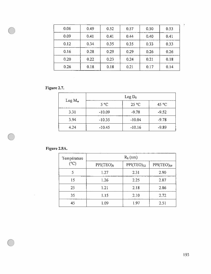
o

Figure 2.7.

Log D0Log M

5°C 25°C 45°C

3.31 -10.09 -9.78 -9.52

3.94 -10.35 -10.04 -9.78

4.24 -10.45 -10.16 -9.89

Figure 2.$A.

Température Rh (nm)

(°C) PPI(TEO)8 PPI(TEO)32 PPI(TEO)M

5 1.27 2.31 2.90

15 1.26 2.25 2.87

25 1.21 2.18 2.86

35 1.15 2.10 2.72

45 1.09 1.97 2.51

0.06 0.49 0.52 0.57 0.50 0.53

0.09 0.41 0.41 0.44 0.40 0.41

0.12 0.34 0.35 0.35 0.33 0.33

0.16 0.28 0.29 0.29 0.26 0.26

0.20 0.22 0.23 0.24 0.21 0.18

0.26 0.18 0.18 0.21 0.17 0.14

1 r-I Y.)

Figure 2.8B.

Température V

(°C) PPI(TEO)8 PPI(TEO)32 PPI(TEO)64

5 0.54 0.67 0.7

15 0.54 0.67 0.66

25 0.59 0.68 0.69

35 0.56 0.65 0.65

45 0.49 0.55 0.56

Figure 2.9.

l/T Ln D du PPI(TEO)32

(1fK) a b c d

0.0036 -23.84 -24.78 -25.56 -26.51

0.0035 -23.45 -24.37 -25.40 -25.98

0.0034 -23.12 -23.92 -24.79 -25.53

0.0033 -22.82 -23.69 -24.44 -25.19

0.0032 -22.52 -23.46 -24.17 -24.82

a=0.00 g!mLdePVA

b0.03 g!mLdePVA

c0.16glmLdePVA

a = 0.26 gJmL de PVA

194

Figure 2.10.

Ea (kJ/mol)

Échantillonsa b c d

PPI(TEO)s 23.4 24.3 26.3 28.5

PPI(TEO)32 24.1 24.6 27.6 30.9

PPI(TEO)64 24.3 26.3 28.6 33.0

a=0.00 g/mL dePVA

b0.03 g/mLdePVA

c=0.16g/mLdePVA

a0.26WmLdePVA

Figure 2.11.

lIT Lnk132(1 1K) PPI(TEO)8 PPI(TEO)32 PPI(TEO)64

0.0036 -26.27 -28.04 -28.76

0.0035 -25.91 -27.62 -28.06

0.0034 -25.57 -27.15 -27.64

0.0033 -25.25 -26.69 -27.11

0.0032 -24.69 -26.04 -26.45

Figure 3.4.

Échantillons Log Log D0 Log Rh

PGHB-1 5,78 21,61 21,46

PGHB-2 6,44 21,87 21,20

PGHB-3 7,01 22,38 20,68

PGHB-4 7,53 22,65 20,41

195

Figure 3.5.Q

figure 3.5. (Suite)

[PVA] D (x10 m2/s) [PVAj D (x10° m2/s)

(g!mL) PGHB-3 (g!mL) PGHB-4

0 1,92 0 1,46

0,03 1,35 0,03 1,03

0,06 1,03 0,06 0,74

0,09 0,82 0,09 0,61

0,12 0,72 0,12 0,51

0,16 0,61 0,15 0,44

0,20 0,53 0,20 0,36

0,25 0,46 0,25 0,31

0,31 0,37 0,31 0,26

[PVA] D (x10’° m2/s) [PVA] D (x10’° m2/s)

(g!mL) PGHB-1 (g!mL) PGHB-2

0 4,12 0 3,19

0,03 3,22 0,03 2,42

0,06 2,66 0,06 1,88

0,09 2,23 0,09 1,46

0,12 1,92 0,12 1,25

0,14 1,64 0,16 1,1

0,20 1,33 0,20 0,91

0,26 0,98 0,25 0,71

0,32 0,82 0,32 0,6

196

Figure 3.5.

[PVA] D/D0 {PVA] D/D0

(g/mL) PGHB-1 (gJmL) PGHB-2

0 1 0 1

0,03 0,78 0,03 0,76

0,06 0,65 0,06 0,59

0,09 0,54 0,09 0,46

0,12 0,47 0,12 0,39

0,14 0,40 0,16 0,35

0,20 0,32 0,20 0,29

0,26 0,24 0,25 0,22

0,32 0,20 0,32 0,19

figure 3.5. (Suite)

[PVA] D/D0 [PVA] D/D0

(g/mL) PGHB-3 (g!mL) PGHB-4

0 1 0 1

0,03 0,70 0,03 0,71

0,06 0,54 0,06 0,51

0,09 0,43 0,09 0,42

0,12 0,38 0,12 0,35

0,16 0,32 0,15 0,30

0,20 0,28 0,20 0,25

0,25 0,24 0,25 0,21

0,31 0,19 0,31 0,18

197

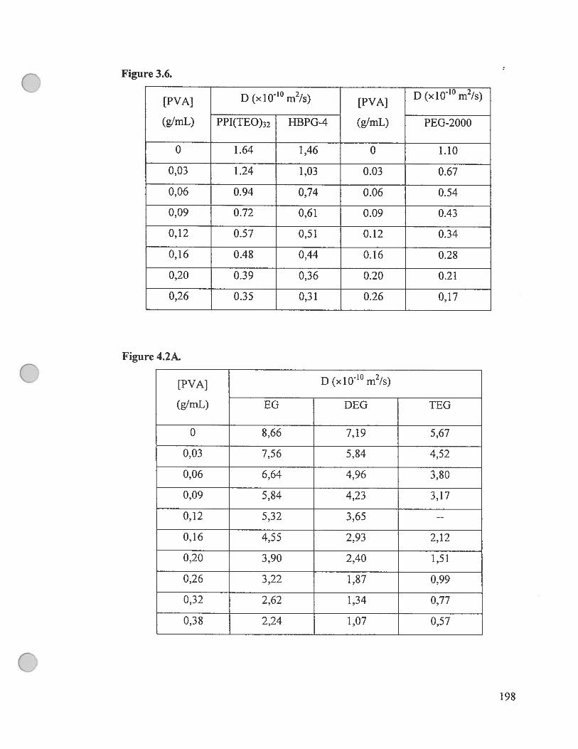
figure 3.6.

[PVA] D (x10’° m2/s) [PVA] D (x10’° m2/s)

(g!mL) PPI(TEO)32 HBPG-4 (g!mL) PEG-2000

0 1.64 1,46 0 1.10

0,03 1.24 1,03 0.03 0.67

0,06 0.94 0,74 0.06 0.54

0,09 0.72 0,61 0.09 0.43

0,12 0.57 0,51 0.12 0.34

0,16 0.48 0,44 0.16 0.28

0,20 0.39 0,36 0.20 0.21

0,26 0.35 0,31 0.26 0,17

Figure 4.2A.

[PVAJ D (x10 m2/s)

(g!mL) EG DEG TEG

0 8,66 7,19 5,67

0,03 7,56 5,84 4,52

0,06 6,64 4,96 3,80

0,09 5,84 4,23 3,17

0,12 5,32 3,65 --

0,16 4,55 2,93 2,12

0,20 3,90 2,40 1,51

0,26 3,22 1,87 0,99

0,32 2,62 1,34 0,77

0,38 2,24 1,07 0,57

198

Figure 4.3A.

[PVA] D (x10’° m2/s)

(g!mL) EG EGMe EGMe2 TEG TEGMe TEGMe2

0 8,66 7,88 7,56 5,67 5,23 5,15

0,03 7,56 7,05 6,7$ 4,52 4,56 4,40

0,06 6,64 6,37 5,88 3,80 4,02 3,94

0,09 5,84 5,76 5,39 3,17 3,41 3,34

0,12 5,32 5,11 4,82 -- 3,13 3,08

0,16 4,55 4,54 4,26 2,12 2,72 2,69

0,20 3,90 4,06 3,80 1,51 2,32 2,26

0,26 3,22 3,29 3,37 0,99 1,99 1,95

0,32 2,62 2,93 2,86 0,77 1,64 1,61

0,3$ 2,24 2,48 2,33 0,57 1,39 1,32

Figure 4.4A.

[PDEA] D (x10’° m2/s)

(g!mL) TEG TEGMe TEGMe2

0 5,67 5,23 5,15

0,03 4,52 4,66 4,44

0,06 3,80 4,17 3,98

0,09 3,17 3,70 3,54

0,12 -- 3,41 3,22

0,16 2,12 2,92 2,79

0,20 1,51 2,56 2,49

0,26 0,99 2,11 1,98

0,32 0,77 1,80 1,65

0,38 0,57 1,49 1,44

199

Figure 4.6k

[PVAJ D (x1010 m2/s)

(g/mL) EG EDA HAc

0 8,66 8,26 10,12

0,03 7,56 7,27 8,71

0,06 6,64 6,10 7,77

0,09 5,84 5,59 6,87

0,12 5,32 5,01 6,27

0,16 4,55 4,41 5,47

0,20 3,90 3,84 4,83

0,26 3,22 3,02 4,12

0,32 2,62 2,66 3,40

0,38 2,24 2,22 3,03

Figure 4.7A.

{PVA] D (x10’° m2/s)

(g/mL) 25 °C 30 °C 35 °C 40 °C 45 °C

0 8,66 9,86 11,09 12,61 14,88

0,03 7,56 8,68 9,74 10,98 12,81

0,06 6,64 7,70 8,81 10,11 11,50

0,09 5,84 6,92 7,95 2,90 10,25

0,12 5,32 6,24 7,03 7,98 9,22

0,16 4,55 5,52 6,22 7,07 7,98

0,20 3,90 4,79 5,48 6,18 7,18

0,26 3,22 4,04 4,61 5,35 5,96

0,32 2,62 3,27 3,80 4,56 5,21

0,38 2,24 2,67 3,41 3,85 4,56

200

Figure 4.8A.

DEG (x10’° m2/s)[Polymer]

(g/mL) PVA PDEA PAA PAAm

0 8,66 8,66 8,66 8,66

0,03 7,56 7,72 8,16 8,33

0,06 6,64 7,05 7,55 7,86

0,12 5,32 5,91 6,69 7,17

0,2 3,90 4,85 5,87 6,43

0,26 3,22 4,13 5,25 5,93

201

Annexe C: Liste de publication

En préparation:

[12]. W.E. Baille, J. Luo, G. Giguère, X.X. Zhu, Study ofthe diffusion process of

asymmetric PEG stars with cholane core, Macromolecules, 2004.

Soumis:

[11]. W.E. Baille, L. Masaro, M. Gauthier, X.X. Zhu, Study ofDffusant/Polymer

Matrix interactions by FfG NMR Spectroscopy, J. Polym. Sci. Polym. Phys.,

2004.

Publiés:

[10]. W.E. Baille, X.X. Zhu, S. Fomine, Study ofSefDffusion of Hyperbranched

Folyglycidols in Foly(vinyl alcohol) Solutions and Gels by Pulsed field

Gradient NMR Spectroscopy, Macromolecules, 2004, 37, 8569-8576.

[9]. D. Avoce, W.E. Baille, X.X. Zhu, N-alkylacrylamide copolymers with

(meth)acrylamide derivatives of cholic acid: solution properties and

aggregation, e-Polymers, 2004, no. 007.

[8]. C. Malveau, W.E. Baille, X.X. Zhu, W.T. Ford, Molecular dynamics of

hydrophilic poly(propylene imine) dendrimers in aqueous solutions by ‘H

NMR relaxation, J. Polym. Sci., Part B: Polymer Physics, 2003, 41, 2968-

2974.

[7]. W.E. Baille, C. Malveau, X.X. Zhu, Y.H. Kim, W.T. ford, Seif-dffusion

measurements of hydrophilic poly(propylene imine) dendrimers in poly(vinyl

alcohol) solutions and gels by pulsed field gradient NMR spectroscopy,

Macromolecules, 2003, 36, 839-847.

[6]. C. Malveau, W.E. Baille, X.X. Zhu, R.H. Marchessault, NMR imaging ofhigh

amylose starch tablets: 2. effect of tablet size, Biomacromolecules, 2002, 3,

1249-1254.

202

[5]. W.E. Baille, C. Malveau, X.X. Zhu, R.H. Marchessault, NMR imaging ofhigh

amylose starch tablets: 1. swelling and water uptake, Biomacromolecules,

2002, 3, 214 -218.

[4]. M. Nichifor, X.X. Zhu, W. Baille, D. Cristea, A. Carpov, Bile acid

sequestrants based on cationic dextran hydrogel microspheres. 2. influence of

the length of aikyl substituents at the amino groups of the sorbents on the

sorption ofbile salts, J. Pharm. Sci., 2001, 90, 68 1-689.

[3]. L. Masaro, W.E. Baille, X.X. Zhu, Interaction of ethylene glycol with

poly(vinyl aÏcohol) in aqueous systems as studied by NMR spectroscopy,

Polymer Preprint, 2000, 4], 62-63.

[2]. W.E. Baille, W.Q. Huang, M. Nichifor, X.X. Zhu, functionalized ficyclodextrin polymers for the sorption of bile salts, J. Macromolecular Sci.,

Part A: Pure and Applied and Chemistry, 2000, 37, 667-690.

[1]. L. Masaro, M. Ousalem, W.E. Baille, D. Lessard, X.X. Zhu, $4fdiffusion of

solvents and solute probes in polymer solutions and gels of selected

hydrophilic polymers, Macromolecules, 1999, 32, 4375-4382.

203

Chapitre 4 : Les résultats obtenus par la rhéologie concernant le concentration

critique d’enchevêtrement (c*)

Nous avons déterminé le c de l’alcool polyvinylique (PVA) (M de 52000 et

un degré d’hydrolyse de plus de 99%) par rhéologie en étudiant une dizaine de

concentrations de PVA entre 2.5 et 25 % (jcourcentage massique). Pour l’expérience,

on a travaillé en mode flux continu et une vitesse de cisaillement entre 0.1 s et 1000

s a été nécessaire. Pour la détermination de la viscosité à zéro vitesse de

cisaillement les modèles appropriés ont été utilisés pour les différents lissages. Les

résultats obtenus sont illustrés à la figure ci-dessous.

0.5

0.0>4-

U)g -0.5U)>

-1.0

-1.5

9 -2.0G)N

-2.5-J

-3.01.0

C

0.5 1.5

Log(concentration)

Documents

Université de Montréal RMN par Département de chimie