Embed Size (px)
Citation preview
UNIVERSITA' DEGLI STUDI DI PADOVA
Sede Amministrativa: Università degli Studi di Padova
Dipartimento di Scienze Economiche “Marco Fanno”
SCUOLA DI DOTTORATO DI RICERCA IN ECONOMIA E MANAGEMENT
CICLO XX
THREE ESSAYS ON THE NEW KEYNESIAN PHILLIPS CURVE
Direttore della Scuola: Ch.mo Prof. Guglielmo Weber
Supervisore: Dott. Efrem Castelnuovo
Dottorando: Nico Boldrin
31 luglio 2008

ACKNOWLEDGEMENTS
First of all, I would like to address special thanks to my supervisor, Efrem
Castelnuovo. Working with him has been an extraordinary experience. During my
PhD he has helped me to improve my knowledge in economics. For me he has
represented a sure guide in the labyrinth of economic sciences.
Particular thanks go to my external supervisors during my visiting period at
Birkbeck College University of London, John Driffill and Yunus Aksoy. They
gave me useful suggestions to solve some problems of my research.
Many thanks go to Nunzio Cappuccio, Davide Raggi and Alessandro
Bucciol who contributed to clarify some doubts which I had about econometric
techniques of estimate.
I desire to thank Antonio Nicolò, Guglielmo Weber and Federico Biagi
because during my Department presentations they underlined some critical aspects
of my analyses and were able to indicate valid solutions.
Special thanks go to my parents, Luciano and Maria Luisa, who have always
supported me during my PhD years.
Last, but not least, I will never reserve enough thanks to my girlfriend,
Romana, who has made my life during my PhD a very happy period with her good
cheer and love.

CONTENTS
Abstract 1
Abstract (in Italian) 3
Chapter 1 5
“The New Keynesian Phillips Curve: A Critical Survey”
1. Introduction 5
2. Standard New Keynesian Phillips curve 6
2.1. Taylor’s approach 6
2.2. Rotemberg’s approach 9
2.3. Calvo’s approach 10
2.4. Comments on the standard NKPC 12
3. “Divine coincidence” 12
4. Alternative approaches to solve the “divine coincidence”
problem 13
4.1. Distortion shocks 13
4.2. Alternative structures of wage and price fixing 17
4.3. Cost channel 22
4.4. Real wage rigidities 30
5. Future developments and new challenges 39
6. Conclusions 41
References 43
Chapter 2 47
“Assessing the Relevance of Oil and Exchange Rates in the New Keynesian
Phillips Curve”
1. Introduction 47
2. NKPC: standard model and Blanchard-Galì proposal 48
3. Empirical investigation 50
4. Estimates of the three versions of the New Keynesian Phillips
curve 52
5. Conclusions 55
References 57
Data appendix 59
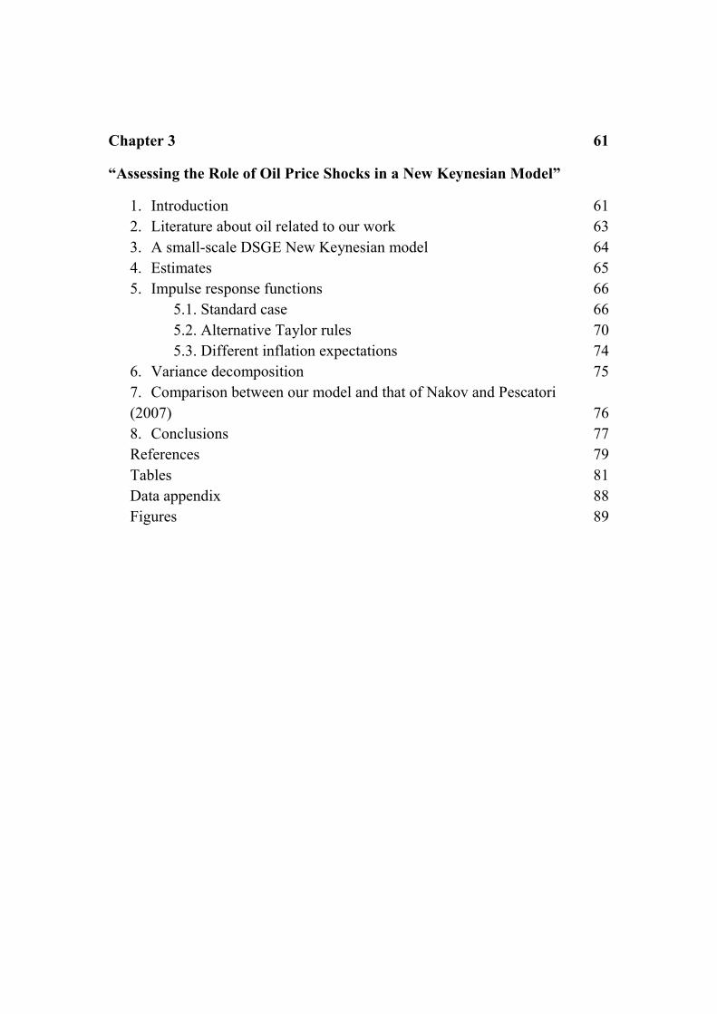
Chapter 3 61
“Assessing the Role of Oil Price Shocks in a New Keynesian Model”
1. Introduction 61
2. Literature about oil related to our work 63
3. A small-scale DSGE New Keynesian model 64
4. Estimates 65
5. Impulse response functions 66
5.1. Standard case 66
5.2. Alternative Taylor rules 70
5.3. Different inflation expectations 74
6. Variance decomposition 75
7. Comparison between our model and that of Nakov and Pescatori
(2007) 76
8. Conclusions 77
References 79
Tables 81
Data appendix 88
Figures 89
1
ABSTRACT
In the recent years the New Keynesian model has become the main tool to
analyse monetary policy and business cycle fluctuations. A fundamental part of
this model is the New Keynesian Phillips curve, which suggests a positive
relationship between current inflation and the output gap.
This PhD thesis is composed by three essays which tackle recent and
controversial aspects of the New Keynesian Phillips curve subject. The first
chapter presents a critical survey about the New Keynesian Phillips curve focusing
on the so-called “divine coincidence” problem. The second chapter proposes an
extension of the Blanchard and Galì New Keynesian Phillips curve and shows that
this new formulation helps to explain inflation dynamics. The third chapter
examines an extended version of the small-scale New Keynesian model a la
Woodford (2003) to assess the role of oil price shocks in influencing inflation and
unemployment volatility.
Chapter 1 analyses the genesis and the evolution of the New Keynesian
Phillips curve, with particular attention to the solutions proposed by the economic
literature to the “divine coincidence” problem, i.e. the absence of a meaningful
trade-off faced by the central bank due to the one-to-one mapping between the
first and the second best output levels. Our work identifies two main approaches
that generate endogenously a trade-off between inflation and the output gap in the
presence of a microfounded shock: the first approach, proposed by Blanchard and
Galì (2007), focuses on real wage rigidities; the second, elaborated by Ravenna
and Walsh (2006), focuses on the cost channel.
Chapter 2 estimates a new version of the New Keynesian Phillips curve
(NKPC) in which real wage stickiness implies the existence of unemployment in
equilibrium (Blanchard and Galì, 2007, Journal of Money, Credit and Banking).
In such model, firms employ a nonproduced input (interpreted as oil) that directly
enters the Phillips curve. We fit this model to U.K. and U.S. data, and we compare
its empirical performance to that offered by the standard NKPC a la Woodford
(2003). The comparison considers the adherence of the results to conventional a
priori. Our results point towards the importance of including both the real
producer price index and the real effective exchange rate in the New Keynesian
2
Phillips curve. In particular, the inclusion of the latter makes unemployment
coefficient significant and forces it to assume a sign coherent with economic
expectation.
Chapter 3 estimates an extended version of the small-scale New Keynesian
model a la Woodford (2003) to account for the impact of oil price shocks on U.S.
inflation and unemployment. We find four main results. First, in the last two
decades, oil price shocks have played an important role in explaining U.S.
inflation fluctuations. Second, stronger reactions to oil price swings than the ones
historically observed would not have improved the stabilization of inflation and
unemployment. Third, the best result in terms of stabilization of inflation and
unemployment is obtained by a “progressive central bank” (i.e. a central bank
which reacts strongly to unemployment and weakly to inflation) in the presence of
oil price shock. Fourth, the more forward-looking the firms are, the more stable
the economy is in the presence of oil price shock.
3
ABSTRACT (IN ITALIAN)
Negli anni recenti il modello neokeynesiano è diventato lo strumento
principale per analizzare la politica monetaria e le fluttuazioni del ciclo
economico. Una parte fondamentale di questo modello è la curva di Phillips
neokeynesiana, la quale suggerisce una relazione positiva tra l’inflazione corrente
e l’output gap (cioè il divario esistente tra il prodotto corrente e il prodotto
naturale). Questa tesi di dottorato è composta da tre saggi che affrontano aspetti
recenti e controversi inerenti il tema della curva di Phillips neokeynesiana. Il
primo capitolo presenta una survey critica relativa alla curva di Phillips
neokeynesiana mettendo a fuoco il cosiddetto problema della “divina
coincidenza”. Il secondo propone un’estensione della curva di Phillips
neokeynesiana di Blanchard e Galì e dimostra che questa nuova formulazione
aiuta a spiegare le dinamiche dell’inflazione. Il terzo esamina una versione estesa
del modello neokeynesiano standard (Woodford (2003)) per valutare quale ruolo
rivestono gli shock sul prezzo del petrolio nell’influenzare la volatilità
dell’inflazione e della disoccupazione.
Il primo capitolo analizza la genesi e l’evoluzione della curva di Phillips
neokeynesiana con particolare attenzione alle soluzioni proposte dalla letteratura
economica al problema della “divina coincidenza” (cioè l’assenza di un
significativo trade-off di fronte alla banca centrale in conseguenza della relazione
costante esistente tra il prodotto efficiente e il prodotto naturale). Tale lavoro
identifica due principali approcci che generano endogenamente un trade-off tra
l’inflazione e l’output gap in presenza di uno shock microfondato: il primo
approccio, proposto da Blanchard e Galì (2007), si focalizza sulle rigidità del
salario reale; il secondo, elaborato da Ravenna e Walsh (2006), si concentra sul
cost channel (cioè sull’influenza esercitata dal tasso di interesse nominale sul
costo marginale delle imprese).
Il secondo capitolo stima una nuova versione della curva di Phillips
neokeynesiana nella quale la vischiosità del salario reale implica l’esistenza di
disoccupazione in equilibrio (Blanchard and Galì (2007), Journal of Money,
Credit and Banking). In tale modello le imprese impiegano un fattore di
produzione non prodotto (interpretato come petrolio) che entra direttamente nella
4
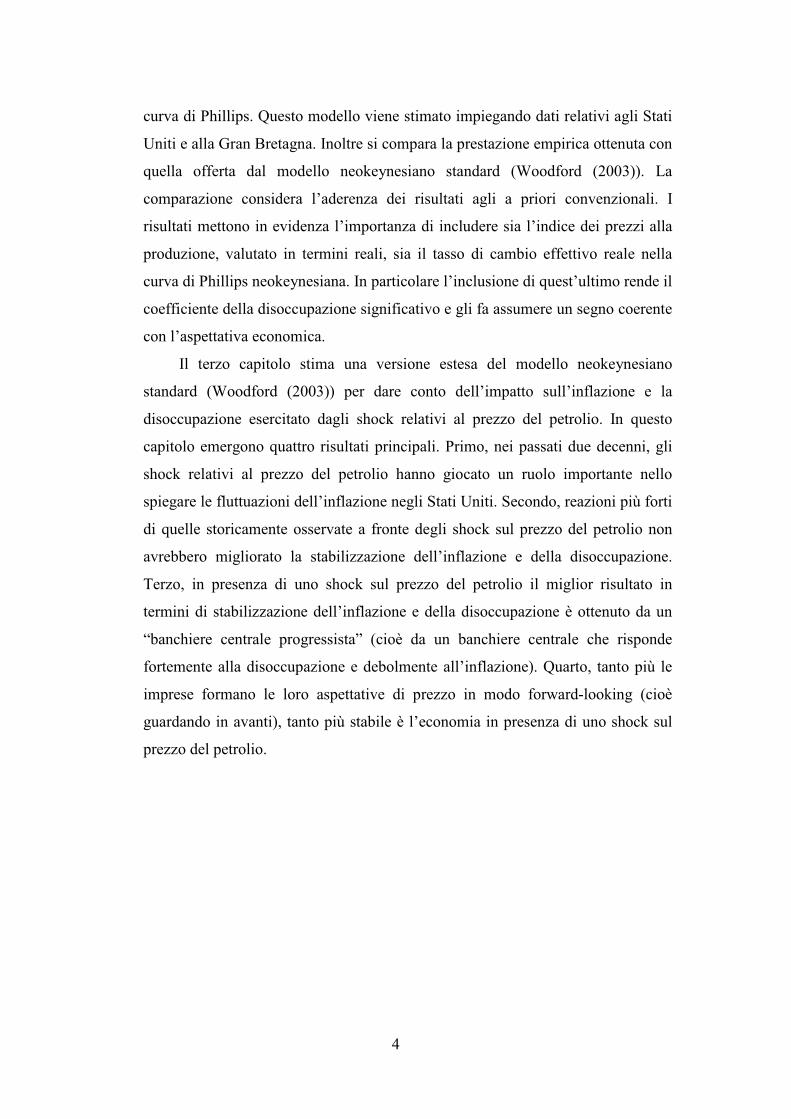
curva di Phillips. Questo modello viene stimato impiegando dati relativi agli Stati
Uniti e alla Gran Bretagna. Inoltre si compara la prestazione empirica ottenuta con
quella offerta dal modello neokeynesiano standard (Woodford (2003)). La
comparazione considera l’aderenza dei risultati agli a priori convenzionali. I
risultati mettono in evidenza l’importanza di includere sia l’indice dei prezzi alla
produzione, valutato in termini reali, sia il tasso di cambio effettivo reale nella
curva di Phillips neokeynesiana. In particolare l’inclusione di quest’ultimo rende il
coefficiente della disoccupazione significativo e gli fa assumere un segno coerente
con l’aspettativa economica.
Il terzo capitolo stima una versione estesa del modello neokeynesiano
standard (Woodford (2003)) per dare conto dell’impatto sull’inflazione e la
disoccupazione esercitato dagli shock relativi al prezzo del petrolio. In questo
capitolo emergono quattro risultati principali. Primo, nei passati due decenni, gli
shock relativi al prezzo del petrolio hanno giocato un ruolo importante nello
spiegare le fluttuazioni dell’inflazione negli Stati Uniti. Secondo, reazioni più forti
di quelle storicamente osservate a fronte degli shock sul prezzo del petrolio non
avrebbero migliorato la stabilizzazione dell’inflazione e della disoccupazione.
Terzo, in presenza di uno shock sul prezzo del petrolio il miglior risultato in
termini di stabilizzazione dell’inflazione e della disoccupazione è ottenuto da un
“banchiere centrale progressista” (cioè da un banchiere centrale che risponde
fortemente alla disoccupazione e debolmente all’inflazione). Quarto, tanto più le
imprese formano le loro aspettative di prezzo in modo forward-looking (cioè
guardando in avanti), tanto più stabile è l’economia in presenza di uno shock sul
prezzo del petrolio.
5
CHAPTER 1
“The New Keynesian Phillips Curve:
A Critical Survey”
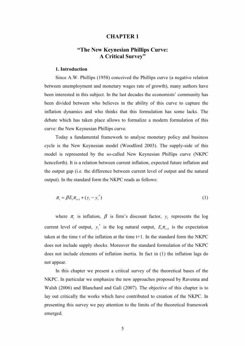
1. Introduction
Since A.W. Phillips (1958) conceived the Phillips curve (a negative relation
between unemployment and monetary wages rate of growth), many authors have
been interested in this subject. In the last decades the economists’ community has
been divided between who believes in the ability of this curve to capture the
inflation dynamics and who thinks that this formulation has some lacks. The
debate which has taken place allows to formalize a modern formulation of this
curve: the New Keynesian Phillips curve.
Today a fundamental framework to analyse monetary policy and business
cycle is the New Keynesian model (Woodford 2003). The supply-side of this
model is represented by the so-called New Keynesian Phillips curve (NKPC
henceforth). It is a relation between current inflation, expected future inflation and
the output gap (i.e. the difference between current level of output and the natural
output). In the standard form the NKPC reads as follows:
*
1 ( )t t t t tE y yπ β π += + − (1)
where tπ is inflation, β is firm’s discount factor, ty represents the log
current level of output, *
ty is the log natural output, 1t tE π + is the expectation
taken at the time t of the inflation at the time t+1. In the standard form the NKPC
does not include supply shocks. Moreover the standard formulation of the NKPC
does not include elements of inflation inertia. In fact in (1) the inflation lags do
not appear.
In this chapter we present a critical survey of the theoretical bases of the
NKPC. In particular we emphasize the new approaches proposed by Ravenna and
Walsh (2006) and Blanchard and Galì (2007). The objective of this chapter is to
lay out critically the works which have contributed to creation of the NKPC. In
presenting this survey we pay attention to the limits of the theoretical framework
emerged.
6
The chapter is organised as follows: Section 2 analyses the theoretical bases
of the standard NKPC. In Section 3 we discuss the “divine coincidence” problem
of the standard formulation of the NKPC, i.e. the absence of a trade-off between
the stabilization of inflation and the stabilization of the welfare-relevant output
gap. Section 4 presents the different solutions that many authors have proposed to
solve the “divine coincidence” problem. Section 5 proposes some promising
avenues to follow to develop the NKPC. Section 6 concludes.
2. Standard New Keynesian Phillips curve
The rational expectations revolution, led by Lucas (1976), imposed a new
challenge to the Keynesian economists: the necessity to integrate the business
cycle analysis of the short-run, characterized by the presence of nominal rigidities,
in a framework in which the economic agents have rational expectations.
This challenge was taken up by important authors. These economists built a
new framework which, today, is the most important instrument to analyse the
monetary policy. This framework was called New Keynesian model. It is a
stochastic and dynamic general equilibrium model. A fundamental block of this
model is the NKPC. Three authors have contributed in fundamental way to model
the standard NKPC: John Taylor (1979, 1980), Julio Rotemberg (1982, 1982a)
and Guillermo Calvo (1983).1 In the next subsections we explore these three
approaches to understand the basic structure of the NKPC.
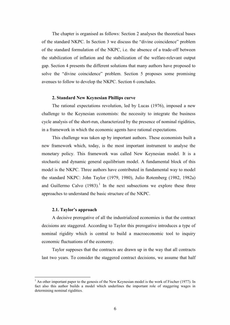
2.1. Taylor’s approach
A decisive prerogative of all the industrialized economies is that the contract
decisions are staggered. According to Taylor this prerogative introduces a type of
nominal rigidity which is central to build a macroeconomic tool to inquiry
economic fluctuations of the economy.
Taylor supposes that the contracts are drawn up in the way that all contracts
last two years. To consider the staggered contract decisions, we assume that half
1 An other important paper to the genesis of the New Keynesian model is the work of Fischer (1977). In
fact also this author builds a model which underlines the important role of staggering wages in
determining nominal rigidities.
7
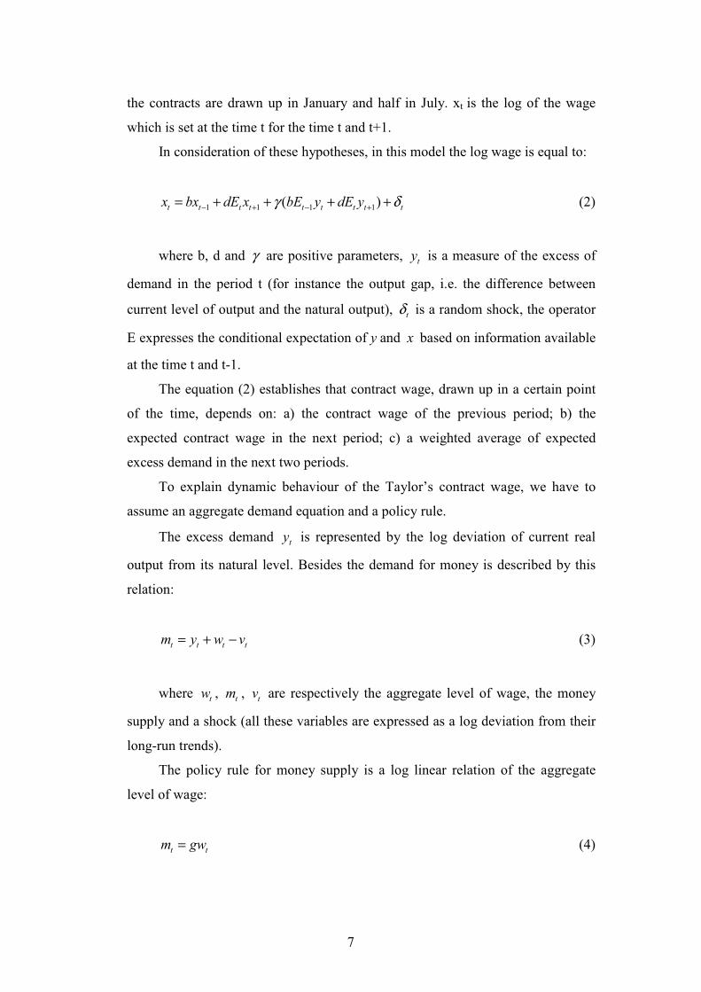
the contracts are drawn up in January and half in July. xt is the log of the wage
which is set at the time t for the time t and t+1.
In consideration of these hypotheses, in this model the log wage is equal to:
1 1 1 1( )t t t t t t t t tx bx dE x bE y dE yγ δ− + − += + + + + (2)
where b, d and γ are positive parameters, ty is a measure of the excess of
demand in the period t (for instance the output gap, i.e. the difference between
current level of output and the natural output), tδ is a random shock, the operator
E expresses the conditional expectation of y and x based on information available
at the time t and t-1.
The equation (2) establishes that contract wage, drawn up in a certain point
of the time, depends on: a) the contract wage of the previous period; b) the
expected contract wage in the next period; c) a weighted average of expected
excess demand in the next two periods.
To explain dynamic behaviour of the Taylor’s contract wage, we have to
assume an aggregate demand equation and a policy rule.
The excess demand ty is represented by the log deviation of current real
output from its natural level. Besides the demand for money is described by this
relation:
t t t tm y w v= + − (3)
where tw , tm , tv are respectively the aggregate level of wage, the money
supply and a shock (all these variables are expressed as a log deviation from their
long-run trends).
The policy rule for money supply is a log linear relation of the aggregate
level of wage:
t tm gw= (4)
8
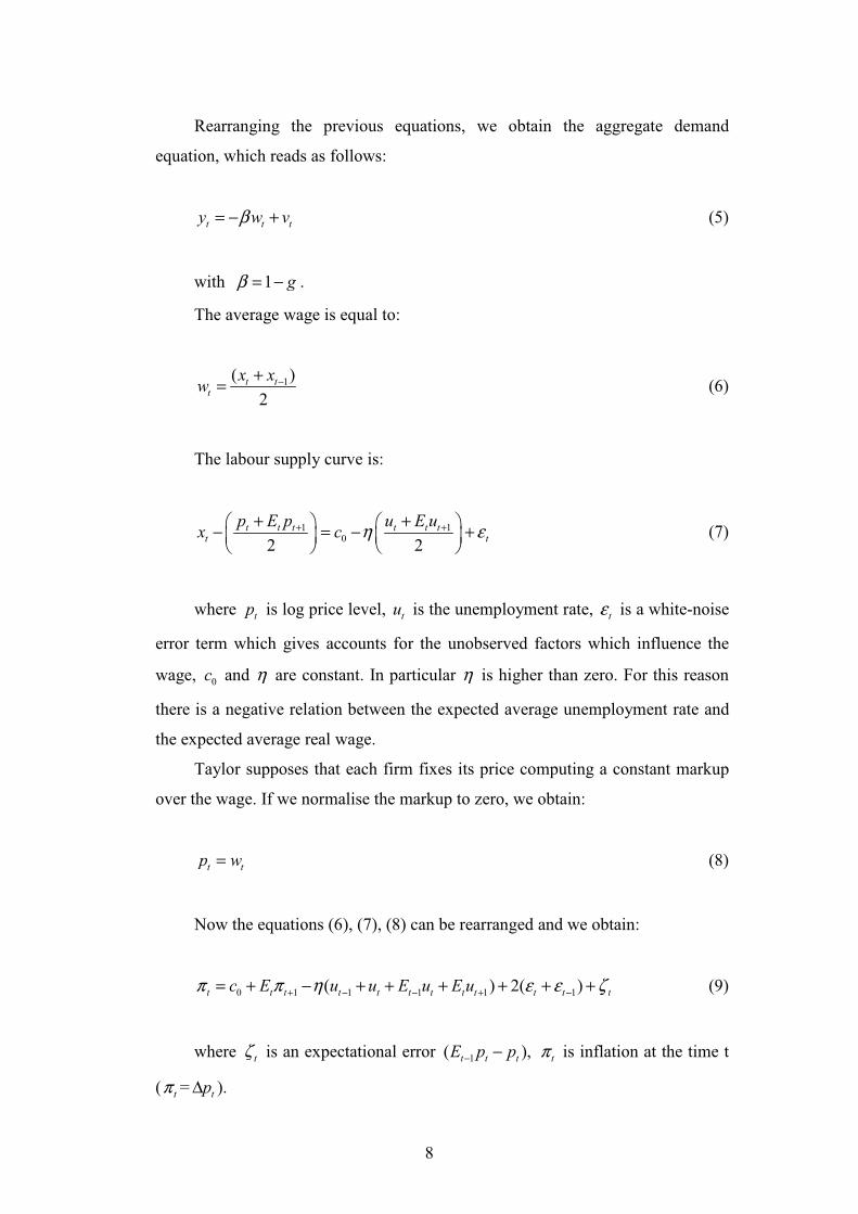
Rearranging the previous equations, we obtain the aggregate demand
equation, which reads as follows:
t t ty w vβ= − + (5)
with 1 gβ = − .
The average wage is equal to:
1( )
2
t tt
x xw −+
= (6)
The labour supply curve is:
1 10
2 2
t t t t t tt t
p E p u E ux c η ε+ ++ +
− = − +
(7)
where tp is log price level, tu is the unemployment rate, tε is a white-noise
error term which gives accounts for the unobserved factors which influence the
wage, 0c and η are constant. In particular η is higher than zero. For this reason
there is a negative relation between the expected average unemployment rate and
the expected average real wage.
Taylor supposes that each firm fixes its price computing a constant markup
over the wage. If we normalise the markup to zero, we obtain:
t tp w= (8)
Now the equations (6), (7), (8) can be rearranged and we obtain:
0 1 1 1 1 1( ) 2( )t t t t t t t t t t t tc E u u E u E uπ π η ε ε ζ+ − − + −= + − + + + + + + (9)
where tζ is an expectational error 1( ),t t tE p p− − tπ is inflation at the time t
( tπ = tp∆ ).
9
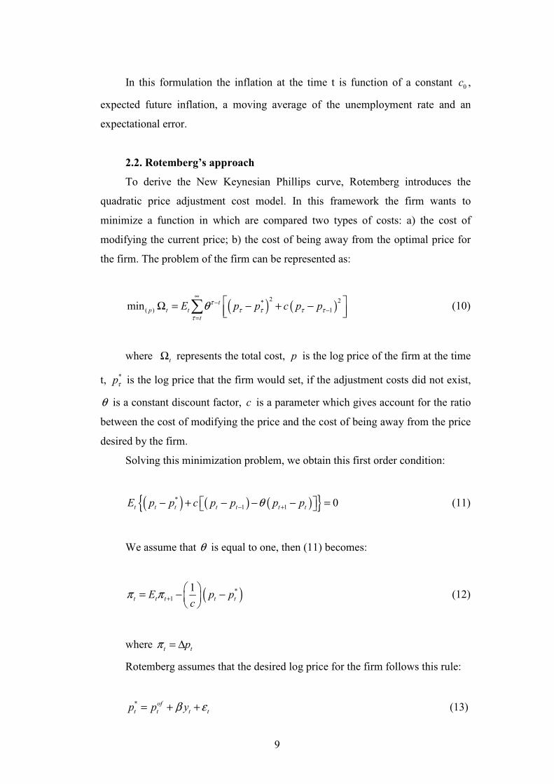
In this formulation the inflation at the time t is function of a constant 0c ,
expected future inflation, a moving average of the unemployment rate and an
expectational error.
2.2. Rotemberg’s approach
To derive the New Keynesian Phillips curve, Rotemberg introduces the
quadratic price adjustment cost model. In this framework the firm wants to
minimize a function in which are compared two types of costs: a) the cost of
modifying the current price; b) the cost of being away from the optimal price for
the firm. The problem of the firm can be represented as:
( ) ( )2 2*
( ) 1min t
p t t
t
E p p c p pττ τ τ τ
τ
θ∞
−−
=
Ω = − + − (10)
where tΩ represents the total cost, p is the log price of the firm at the time
t, *pτ is the log price that the firm would set, if the adjustment costs did not exist,
θ is a constant discount factor, c is a parameter which gives account for the ratio
between the cost of modifying the price and the cost of being away from the price
desired by the firm.
Solving this minimization problem, we obtain this first order condition:
( ) ( ) ( ) *
1 1 0t t t t t t tE p p c p p p pθ− +− + − − − = (11)
We assume that θ is equal to one, then (11) becomes:
( )*
1
1t t t t tE p p
cπ π +
= − −
(12)
where t tpπ = ∆
Rotemberg assumes that the desired log price for the firm follows this rule:
* of
t t t tp p yβ ε= + + (13)
10
where ty is the log deviation between current output and the natural output
(i.e. the output gap), of
tp is the price which the other firms set at the time t, β is a
positive parameter and tε is a i.i.d. random error. The equation (13) describes a
positive relation between the optimal price of the firm and the aggregate output.
Because we assume that all firms are identical, we can replace ofp with p
in the equation (13) and rearranging we obtain:
1t
t t t tE yc c
εβπ π +
= + +
(14)
The equation (14) expresses inflation at the time t as a function of expected
future inflation, the output gap and the error term. In particular, when the current
output gap rises, current inflation increases.
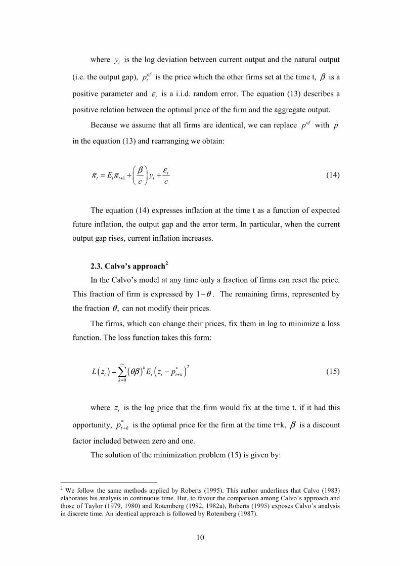
2.3. Calvo’s approach2
In the Calvo’s model at any time only a fraction of firms can reset the price.
This fraction of firm is expressed by 1 θ− . The remaining firms, represented by
the fraction ,θ can not modify their prices.
The firms, which can change their prices, fix them in log to minimize a loss
function. The loss function takes this form:
( ) ( ) ( )2
*
0
k
t t t t k
k
L z E z pθβ∞
+=
= − (15)
where tz is the log price that the firm would fix at the time t, if it had this
opportunity, *t kp + is the optimal price for the firm at the time t+k, β is a discount
factor included between zero and one.
The solution of the minimization problem (15) is given by:
2 We follow the same methods applied by Roberts (1995). This author underlines that Calvo (1983)
elaborates his analysis in continuous time. But, to favour the comparison among Calvo’s approach and
those of Taylor (1979, 1980) and Rotemberg (1982, 1982a), Roberts (1995) exposes Calvo’s analysis
in discrete time. An identical approach is followed by Rotemberg (1987).
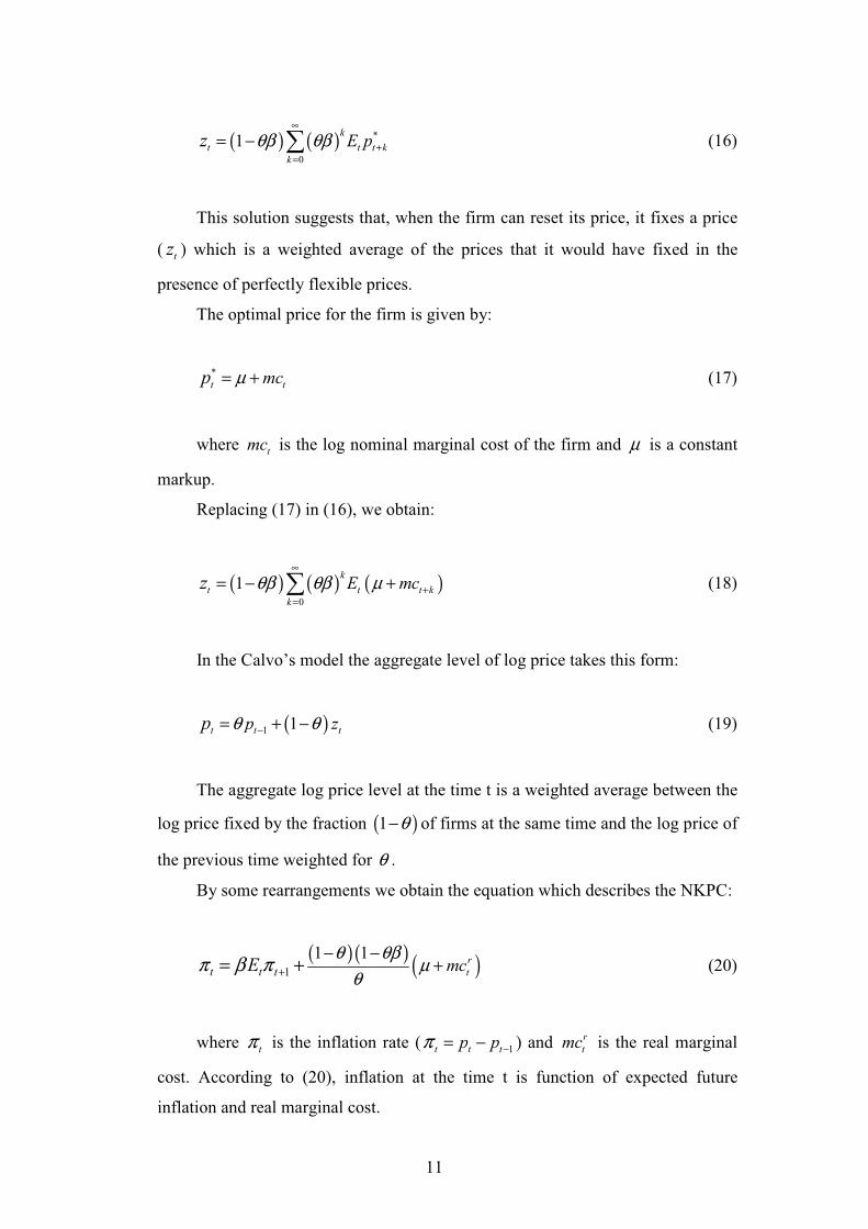
11
( ) ( ) *
0
1k
t t t k
k
E pz θβ θβ∞
+=
= − (16)
This solution suggests that, when the firm can reset its price, it fixes a price
( tz ) which is a weighted average of the prices that it would have fixed in the
presence of perfectly flexible prices.
The optimal price for the firm is given by:
*
t tmcp µ= + (17)
where tmc is the log nominal marginal cost of the firm and µ is a constant
markup.
Replacing (17) in (16), we obtain:
( ) ( ) ( )0
1k
t t t k
k
E mcz θβ θβ µ∞
+=
= − + (18)
In the Calvo’s model the aggregate level of log price takes this form:
( )1 1t t tp zp θ θ−= + − (19)
The aggregate log price level at the time t is a weighted average between the
log price fixed by the fraction ( )1 θ− of firms at the same time and the log price of
the previous time weighted for θ .
By some rearrangements we obtain the equation which describes the NKPC:
( ) ( ) ( )1
1 1r
tt t t mcEθ θβ
µθ
π β π +
− −+= + (20)
where tπ is the inflation rate ( 1t t tp pπ −= − ) and r
tmc is the real marginal
cost. According to (20), inflation at the time t is function of expected future
inflation and real marginal cost.
12
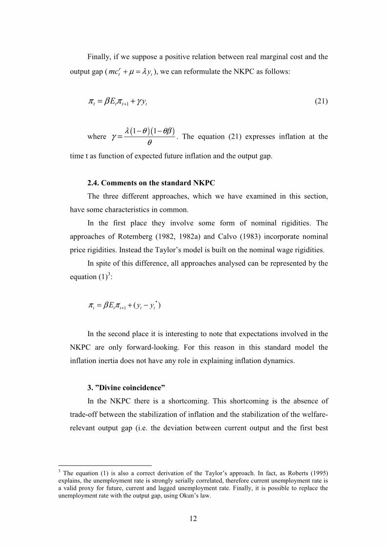
Finally, if we suppose a positive relation between real marginal cost and the
output gap ( t
rt ymc µ λ+ = ), we can reformulate the NKPC as follows:
1 tt t tE yπ β π γ+= + (21)
where ( )( )1 1λ θ θβ
θγ
− −= . The equation (21) expresses inflation at the
time t as function of expected future inflation and the output gap.
2.4. Comments on the standard NKPC
The three different approaches, which we have examined in this section,
have some characteristics in common.
In the first place they involve some form of nominal rigidities. The
approaches of Rotemberg (1982, 1982a) and Calvo (1983) incorporate nominal
price rigidities. Instead the Taylor’s model is built on the nominal wage rigidities.
In spite of this difference, all approaches analysed can be represented by the
equation (1)3:
*
1 ( )t t t t tE y yπ β π += + −
In the second place it is interesting to note that expectations involved in the
NKPC are only forward-looking. For this reason in this standard model the
inflation inertia does not have any role in explaining inflation dynamics.
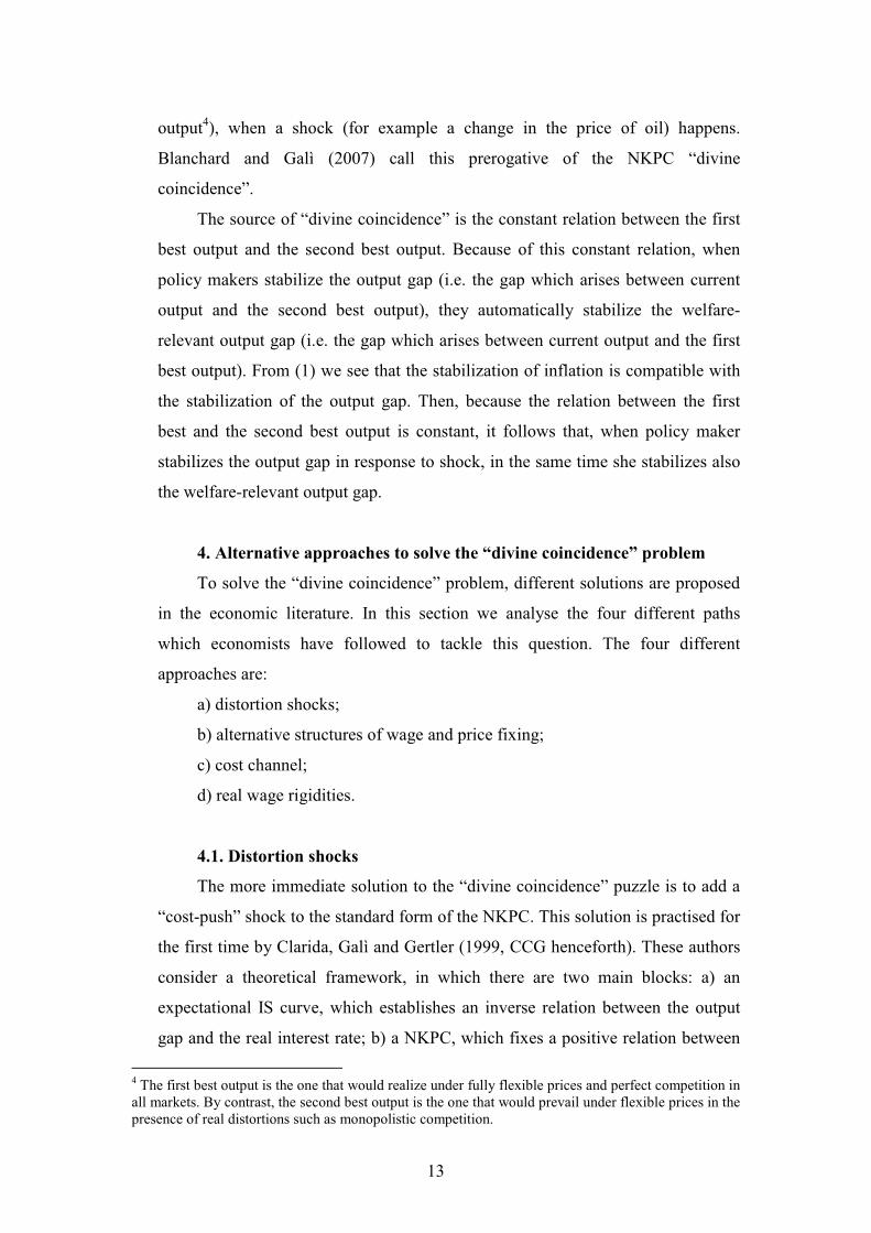
3. ”Divine coincidence”
In the NKPC there is a shortcoming. This shortcoming is the absence of
trade-off between the stabilization of inflation and the stabilization of the welfare-
relevant output gap (i.e. the deviation between current output and the first best
3 The equation (1) is also a correct derivation of the Taylor’s approach. In fact, as Roberts (1995)
explains, the unemployment rate is strongly serially correlated, therefore current unemployment rate is
a valid proxy for future, current and lagged unemployment rate. Finally, it is possible to replace the
unemployment rate with the output gap, using Okun’s law.
13
output4), when a shock (for example a change in the price of oil) happens.
Blanchard and Galì (2007) call this prerogative of the NKPC “divine
coincidence”.
The source of “divine coincidence” is the constant relation between the first
best output and the second best output. Because of this constant relation, when
policy makers stabilize the output gap (i.e. the gap which arises between current
output and the second best output), they automatically stabilize the welfare-
relevant output gap (i.e. the gap which arises between current output and the first
best output). From (1) we see that the stabilization of inflation is compatible with
the stabilization of the output gap. Then, because the relation between the first
best and the second best output is constant, it follows that, when policy maker
stabilizes the output gap in response to shock, in the same time she stabilizes also
the welfare-relevant output gap.
4. Alternative approaches to solve the “divine coincidence” problem
To solve the “divine coincidence” problem, different solutions are proposed
in the economic literature. In this section we analyse the four different paths
which economists have followed to tackle this question. The four different
approaches are:
a) distortion shocks;
b) alternative structures of wage and price fixing;
c) cost channel;
d) real wage rigidities.
4.1. Distortion shocks
The more immediate solution to the “divine coincidence” puzzle is to add a
“cost-push” shock to the standard form of the NKPC. This solution is practised for
the first time by Clarida, Galì and Gertler (1999, CCG henceforth). These authors
consider a theoretical framework, in which there are two main blocks: a) an
expectational IS curve, which establishes an inverse relation between the output
gap and the real interest rate; b) a NKPC, which fixes a positive relation between
4 The first best output is the one that would realize under fully flexible prices and perfect competition in
all markets. By contrast, the second best output is the one that would prevail under flexible prices in the
presence of real distortions such as monopolistic competition.
14
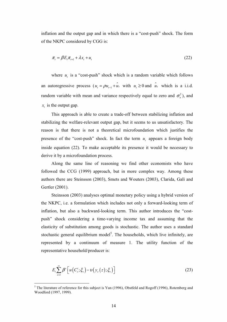
inflation and the output gap and in which there is a “cost-push” shock. The form
of the NKPC considered by CGG is:
1t t t t tE x uπ β π λ+= + + (22)
where tu is a “cost-push” shock which is a random variable which follows
an autoregressive process ( 1 tt tu u uρ −= + with 0tu ≥ and tu which is a i.i.d.
random variable with mean and variance respectively equal to zero and 2
uσ ), and
tx is the output gap.
This approach is able to create a trade-off between stabilizing inflation and
stabilizing the welfare-relevant output gap, but it seems to us unsatisfactory. The
reason is that there is not a theoretical microfoundation which justifies the
presence of the “cost-push” shock. In fact the term tu appears a foreign body
inside equation (22). To make acceptable its presence it would be necessary to
derive it by a microfoundation process.
Along the same line of reasoning we find other economists who have
followed the CCG (1999) approach, but in more complex way. Among these
authors there are Steinsson (2003), Smets and Wouters (2003), Clarida, Galì and
Gertler (2001).
Steinsson (2003) analyses optimal monetary policy using a hybrid version of
the NKPC, i.e. a formulation which includes not only a forward-looking term of
inflation, but also a backward-looking term. This author introduces the “cost-
push” shock considering a time-varying income tax and assuming that the
elasticity of substitution among goods is stochastic. The author uses a standard
stochastic general equilibrium model5. The households, which live infinitely, are
represented by a continuum of measure 1. The utility function of the
representative household/producer is:
( ) ( )( ); ;s i
t s s s s
s t
E u C y zβ ξ υ ξ∞
=
− (23)
5 The literature of reference for this subject is Yun (1996), Obstfeld and Rogoff (1996), Rotemberg and
Woodford (1997, 1999).
15
Where β is a discount factor, sξ is a vector of shocks to households’ tastes
and production aptitude, i
sC is household i’s consumption of a composite
consumption good6, ( )sy z is the differentiated good that the household i
produces.
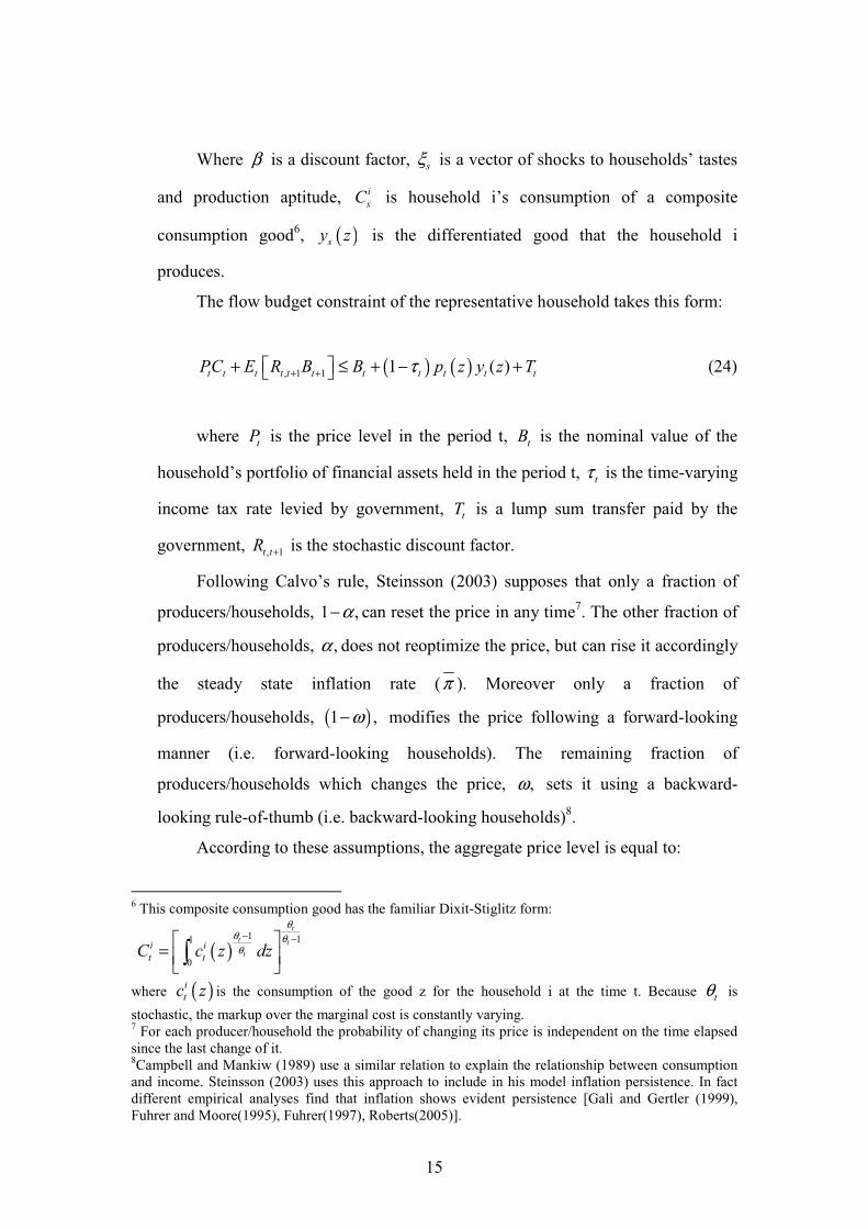
The flow budget constraint of the representative household takes this form:
( ) ( ), 1 1 1 ( )t t t t t t t t t t tPC E R B B p z y z Tτ+ + + ≤ + − + (24)
where tP is the price level in the period t, tB is the nominal value of the
household’s portfolio of financial assets held in the period t, tτ is the time-varying
income tax rate levied by government, tT is a lump sum transfer paid by the
government, , 1t tR + is the stochastic discount factor.
Following Calvo’s rule, Steinsson (2003) supposes that only a fraction of
producers/households, 1 ,α− can reset the price in any time7. The other fraction of
producers/households, ,α does not reoptimize the price, but can rise it accordingly
the steady state inflation rate (π ). Moreover only a fraction of
producers/households, ( )1 ,ω− modifies the price following a forward-looking
manner (i.e. forward-looking households). The remaining fraction of
producers/households which changes the price, ,ω sets it using a backward-
looking rule-of-thumb (i.e. backward-looking households)8.
According to these assumptions, the aggregate price level is equal to:
6 This composite consumption good has the familiar Dixit-Stiglitz form:
( )1 11
0
t
t t
ti i
t tC c z dz
θθ θθ
− − =
where ( )i
tc z is the consumption of the good z for the household i at the time t. Because tθ is
stochastic, the markup over the marginal cost is constantly varying. 7 For each producer/household the probability of changing its price is independent on the time elapsed
since the last change of it. 8Campbell and Mankiw (1989) use a similar relation to explain the relationship between consumption
and income. Steinsson (2003) uses this approach to include in his model inflation persistence. In fact
different empirical analyses find that inflation shows evident persistence [Galì and Gertler (1999),
Fuhrer and Moore(1995), Fuhrer(1997), Roberts(2005)].
16
( ) ( ) ( )( ) ( ) ( )1
1 1 1 1
1 1 1 1t t t tf b
t t t tP P p pθ θ θ θ
α π α ω α ω− − − −
− = + − − + −
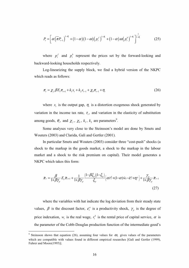
(25)
where f
tp and b
tp represent the prices set by the forward-looking and
backward-looking households respectively.
Log-linearizing the supply block, we find a hybrid version of the NKPC
which reads as follows:
1 1 2 1 1t f t t t t b t tE k x k xπ χ β π χ π η+ − −= + + + + (26)
where tx is the output gap, tη is a distortion exogenous shock generated by
variation in the income tax rate, ,tτ and variation in the elasticity of substitution
among goods, ,tθ and fχ , bχ , 1k , 2k are parameters9.
Some analyses very close to the Steinsson’s model are done by Smets and
Wouters (2003) and Clarida, Galì and Gertler (2001).
In particular Smets and Wouters (2003) consider three “cost-push” shocks (a
shock to the markup in the goods market, a shock to the markup in the labour
market and a shock to the risk premium on capital). Their model generates a
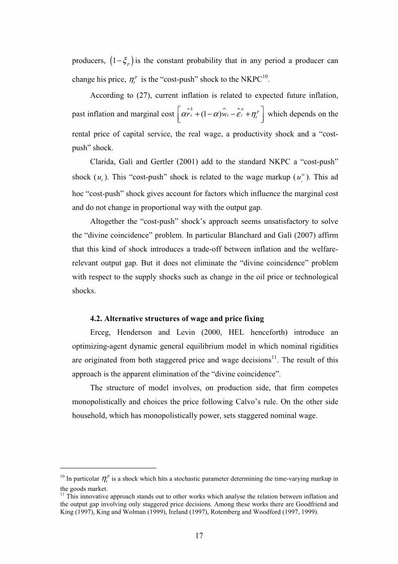
NKPC which takes this form:
( )( )
1 1
1 11(1 )
1 1 1p p pak p
tt t t t tt tp p p p
E r wβξ ξ γβ
π π α α ε η πβγ βγ ξ βγ
+ −
− −= + + − − + +
+ + +
(27)
where the variables with hat indicate the log deviation from their steady state
values, β is the discount factor, a
tε is a productivity shock, pγ is the degree of
price indexation, tw is the real wage, k
tr is the rental price of capital service, α is
the parameter of the Cobb-Douglas production function of the intermediate good’s
9 Steinsson shows that equation (26), assuming four values for ,ω gives values of the parameters
which are compatible with values found in different empirical researches [Galì and Gertler (1999),
Fuhrer and Moore(1995)].
17
producers, ( )1 pξ− is the constant probability that in any period a producer can
change his price, p
tη is the “cost-push” shock to the NKPC10
.
According to (27), current inflation is related to expected future inflation,
past inflation and marginal cost (1 )k a
pt t t tr wα α ε η + − − +
which depends on the
rental price of capital service, the real wage, a productivity shock and a “cost-
push” shock.
Clarida, Galì and Gertler (2001) add to the standard NKPC a “cost-push”
shock ( tu ). This “cost-push” shock is related to the wage markup (t
wu ). This ad
hoc “cost-push” shock gives account for factors which influence the marginal cost
and do not change in proportional way with the output gap.
Altogether the “cost-push” shock’s approach seems unsatisfactory to solve
the “divine coincidence” problem. In particular Blanchard and Galì (2007) affirm
that this kind of shock introduces a trade-off between inflation and the welfare-
relevant output gap. But it does not eliminate the “divine coincidence” problem
with respect to the supply shocks such as change in the oil price or technological
shocks.
4.2. Alternative structures of wage and price fixing
Erceg, Henderson and Levin (2000, HEL henceforth) introduce an
optimizing-agent dynamic general equilibrium model in which nominal rigidities
are originated from both staggered price and wage decisions11
. The result of this
approach is the apparent elimination of the “divine coincidence”.
The structure of model involves, on production side, that firm competes
monopolistically and choices the price following Calvo’s rule. On the other side
household, which has monopolistically power, sets staggered nominal wage.
10
In particolar p
tη is a shock which hits a stochastic parameter determining the time-varying markup in
the goods market. 11
This innovative approach stands out to other works which analyse the relation between inflation and
the output gap involving only staggered price decisions. Among these works there are Goodfriend and
King (1997), King and Wolman (1999), Ireland (1997), Rotemberg and Woodford (1997, 1999).
18
Firms
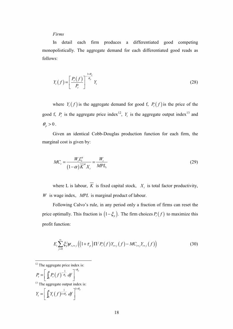
In detail each firm produces a differentiated good competing
monopolistically. The aggregate demand for each differentiated good reads as
follows:
( )( )
1 p
pt
t t
t
P fY f Y
P
θ
θ
+−
=
(28)
where ( )tY f is the aggregate demand for good f, ( )tP f is the price of the
good f, tP is the aggregate price index12
, tY is the aggregate output index13
and
0pθ > .
Given an identical Cobb-Douglas production function for each firm, the
marginal cost is given by:
( )1
t t tt
tt
W L WMC
MPLK X
α
αα
= =−
(29)
where L is labour, K is fixed capital stock, tX is total factor productivity,
W is wage index, MPL is marginal product of labour.
Following Calvo’s rule, in any period only a fraction of firms can reset the
price optimally. This fraction is ( )1 .pξ− The firm choices ( )tP f to maximize this
profit function:
( ) ( ) ( ) ( )( ),
0
1j j
t p t t j p t t j t j t j
j
E P f Y f MC Y fξ ψ τ∞
+ + + +=
+ Π − (30)
12
The aggregate price index is:
( )11
0
p
pt tP P f df
θ
θ
−−
=
13 The aggregate output index is:
( )1
111
0
p
pt tY Y f df
θ
θ
+
+
=
19
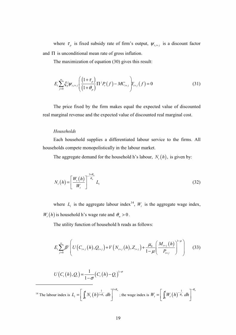
where pτ is fixed subsidy rate of firm’s output, ,t t jψ + is a discount factor
and Π is unconditional mean rate of gross inflation.
The maximization of equation (30) gives this result:
( )( )
( ) ( ),
0
10
1
pj j
t p t t j t t j t j
j p
E P f MC Y fτ
ξ ψθ
∞
+ + +=
+ Π − = +
(31)
The price fixed by the firm makes equal the expected value of discounted
real marginal revenue and the expected value of discounted real marginal cost.
Households
Each household supplies a differentiated labour service to the firms. All
households compete monopolistically in the labour market.
The aggregate demand for the household h’s labour, ( ) ,tN h is given by:
( )( )
1 w
wt
t t
t
W hN h L
W
θ
θ
+−
=
(32)
where tL is the aggregate labour index14
, tW is the aggregate wage index,
( )tW h is household h’s wage rate and 0wθ > .
The utility function of household h reads as follows:
( )( ) ( )( ) ( )1
0
0
, ,1
t jj
t t j t j t j t j
j t j
M hE U C h Q V N h Z
P
µ
µβ
µ
−∞
+
+ + + += +
+ + −
(33)
( )( ) ( )( )11
,1
t t t tU C h Q C h Qσ
σ
−= −
−
14 The labour index is ( )
111
1
0
w
wt tL N h dh
θ
θ
+
+
= ; the wage index is ( )
11
0
w
wt tW W h dh
θ
θ
−−
=
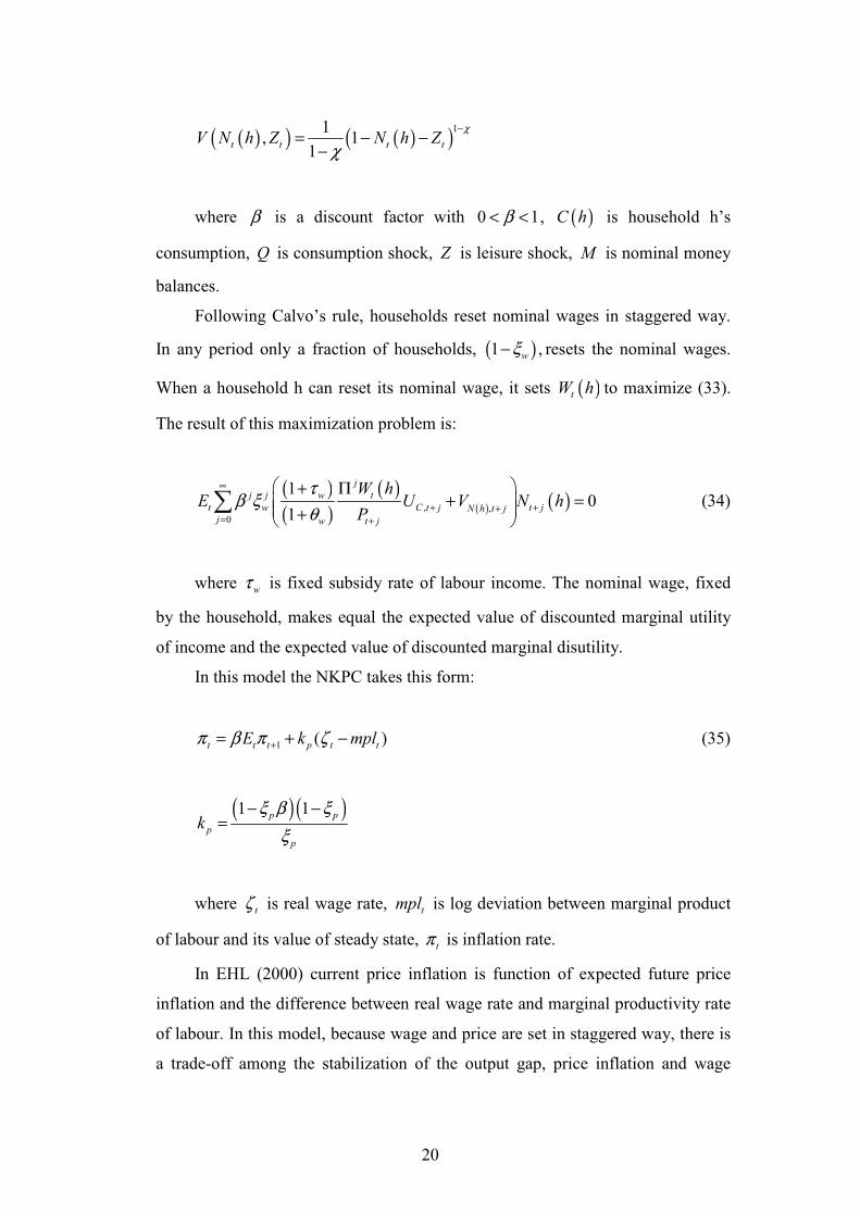
20
( )( ) ( )( )11
, 11
t t t tV N h Z N h Zχ
χ
−= − −
−
where β is a discount factor with 0 1β< < , ( )C h is household h’s
consumption, Q is consumption shock, Z is leisure shock, M is nominal money
balances.
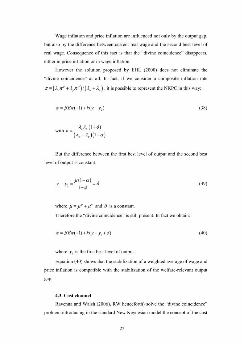
Following Calvo’s rule, households reset nominal wages in staggered way.
In any period only a fraction of households, ( )1 ,wξ− resets the nominal wages.
When a household h can reset its nominal wage, it sets ( )tW h to maximize (33).
The result of this maximization problem is:
( )( )
( )( ) ( ), ,
0
10
1
j
w tj j
t w C t j t jN h t jj w t j
W hE U V N h
P
τβ ξ
θ
∞
+ ++= +
+ Π+ = +
(34)
where wτ is fixed subsidy rate of labour income. The nominal wage, fixed
by the household, makes equal the expected value of discounted marginal utility
of income and the expected value of discounted marginal disutility.
In this model the NKPC takes this form:
1 ( )t t t p t tE k mplπ β π ζ+= + − (35)
( )( )1 1p p
p
p
kξ β ξ
ξ
− −=
where tζ is real wage rate, tmpl is log deviation between marginal product
of labour and its value of steady state, tπ is inflation rate.
In EHL (2000) current price inflation is function of expected future price
inflation and the difference between real wage rate and marginal productivity rate
of labour. In this model, because wage and price are set in staggered way, there is
a trade-off among the stabilization of the output gap, price inflation and wage

21
inflation. Besides HEL (2000) show that it is possible only for one variable among
the output gap, price inflation and wage inflation to have zero variance.
Using Blanchard and Galì terminology (presented in subsection 4.4), we
explain that EHL approach does not eliminate the “divine coincidence” at all15
.
EHL show that, if wages and prices are staggered following Calvo’s rule, a
trade-off between the stabilization of price inflation and the stabilization of the
output gap arises. In EHL model wage inflation is:
( ) ( )1w w w
wE w mrsπ β π λ µ= + − − −
( ) ( )( )1 1w w w
wE w m nπ β π λ α α φ ξ µ= + − − − − + − −
( ) ( ) ( )2 21 11
w w
w wE w w y yφ
π β π λ λα
= + − − + + −
− (36)
where w is current level of real wage, 2w is the second best level of real
wage, y is current level of output, 2y is the second best level of output16
, wµ is
constant desired wage markup, wλ is a coefficient, m represents oil, α is the
share of oil used in production, φ is the slope of the labour supply curve, n
represents labour, mrs is the household’s marginal rate of substitution, ξ is a
preference parameter.
Price inflation is described by this equation:
( ) ( )1p p p
pE mcπ β π λ µ= + + +
( ) ( )( )1 log 1p p p
pE w m nπ β π λ α α α µ= + + − + − − +
( ) ( ) ( )2 211
p p
p pE w w y yα
π β π λ λα
= + + − + −−
(37)
where pλ is a coefficient and pµ is constant desired price markup.
15
The following reasoning is developed by Blanchard and Galì (2007). 16
In this context y2 is the output that would be realized, if there was perfectly flexible prices and wages
but market distortions (i.e. the second best output). By contrast y1 is the output that would be produced
in the presence of perfectly flexible prices and wages and perfect competition in all markets (i.e. the
first best output).
22
Wage inflation and price inflation are influenced not only by the output gap,
but also by the difference between current real wage and the second best level of
real wage. Consequence of this fact is that the “divine coincidence” disappears,
either in price inflation or in wage inflation.
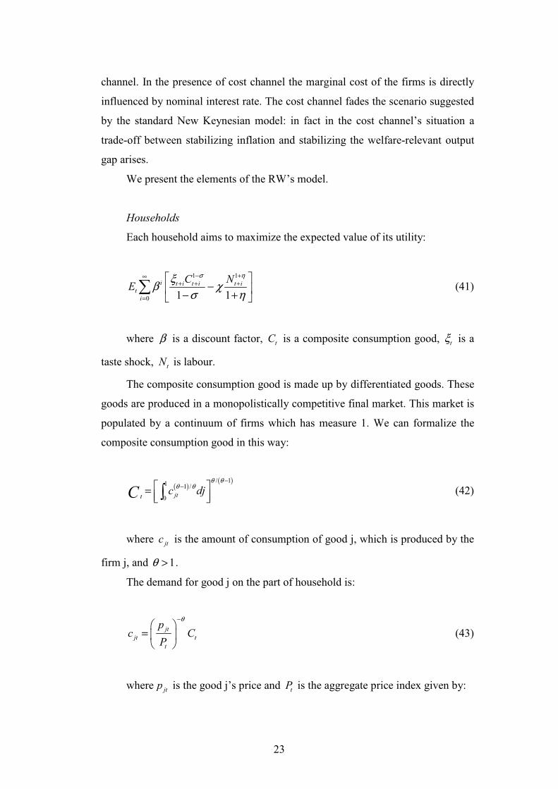
However the solution proposed by EHL (2000) does not eliminate the
“divine coincidence” at all. In fact, if we consider a composite inflation rate
( ) ( )/ ,p w
w p w pπ λ π λ π λ λ≡ + + it is possible to represent the NKPC in this way:
2( 1) ( )E k y yπ β π= + + − (38)
with ( )
( )( )1
1
w p
w p
kλ λ φ
λ λ α
+≡
+ −
But the difference between the first best level of output and the second best
level of output is constant:
( )1 2
1
1y y
µ αδ
φ
−− = ≡
+ (39)
where p wµ µ µ≡ + and δ is a constant.
Therefore the “divine coincidence” is still present. In fact we obtain:
1( 1) ( )E k y yπ β π δ= + + − + (40)
where 1y is the first best level of output.
Equation (40) shows that the stabilization of a weighted average of wage and
price inflation is compatible with the stabilization of the welfare-relevant output
gap.
4.3. Cost channel
Ravenna and Walsh (2006), RW henceforth) solve the “divine coincidence”
problem introducing in the standard New Keynesian model the concept of the cost
23
channel. In the presence of cost channel the marginal cost of the firms is directly
influenced by nominal interest rate. The cost channel fades the scenario suggested
by the standard New Keynesian model: in fact in the cost channel’s situation a
trade-off between stabilizing inflation and stabilizing the welfare-relevant output
gap arises.
We present the elements of the RW’s model.
Households
Each household aims to maximize the expected value of its utility:
1 1
0 1 1
i t i t i t it
i
C NE
σ ηξβ χ
σ η
− +∞+ + +
=
− − +
(41)
where β is a discount factor, tC is a composite consumption good, tξ is a
taste shock, tN is labour.
The composite consumption good is made up by differentiated goods. These
goods are produced in a monopolistically competitive final market. This market is
populated by a continuum of firms which has measure 1. We can formalize the
composite consumption good in this way:
( )( )/ 1
1 1 /
0jtt
c djCθ θ
θ θ−
− = (42)
where jtc is the amount of consumption of good j, which is produced by the
firm j, and 1θ > .
The demand for good j on the part of household is:
jt
jt t
t
pc C
P
θ−
=
(43)
where jtp is the good j’s price and tP is the aggregate price index given by:
24
( )1/ 11
1
0t jtP p dj
θθ
−− =
(44)
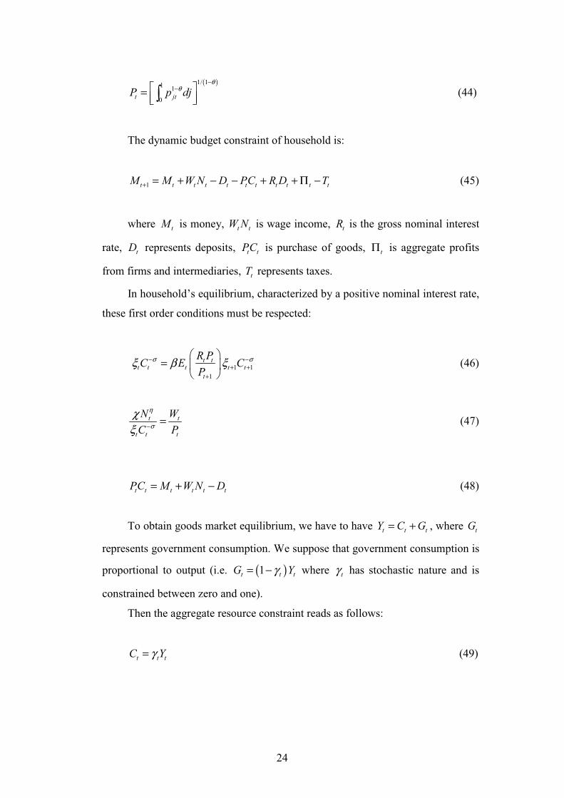
The dynamic budget constraint of household is:
1t t t t t t t t t t tM M W N D PC R D T+ = + − − + + Π − (45)
where tM is money, t tW N is wage income, tR is the gross nominal interest
rate, tD represents deposits, t tPC is purchase of goods, tΠ is aggregate profits
from firms and intermediaries, tT represents taxes.
In household’s equilibrium, characterized by a positive nominal interest rate,
these first order conditions must be respected:
1 1
1
t tt t t t t
t
R PC E C
P
σ σξ β ξ− −+ +
+
=
(46)
t t
t t t
N W
C P
η
σ
χ
ξ −= (47)
t t t t t tPC M W N D= + − (48)
To obtain goods market equilibrium, we have to have t t tY C G= + , where tG
represents government consumption. We suppose that government consumption is
proportional to output (i.e. ( )1t t tG Yγ= − where tγ has stochastic nature and is
constrained between zero and one).
Then the aggregate resource constraint reads as follows:
t t tC Yγ= (49)
25
Firms
Each firm competes monopolistically, following Calvo’s rule. In any time
only a fraction of firms can reset the price. This fraction is equal to 1 ω− . The
firms which can not reset their prices restrict themselves to revise the previous
prices updating them considering the steady state inflation rate.
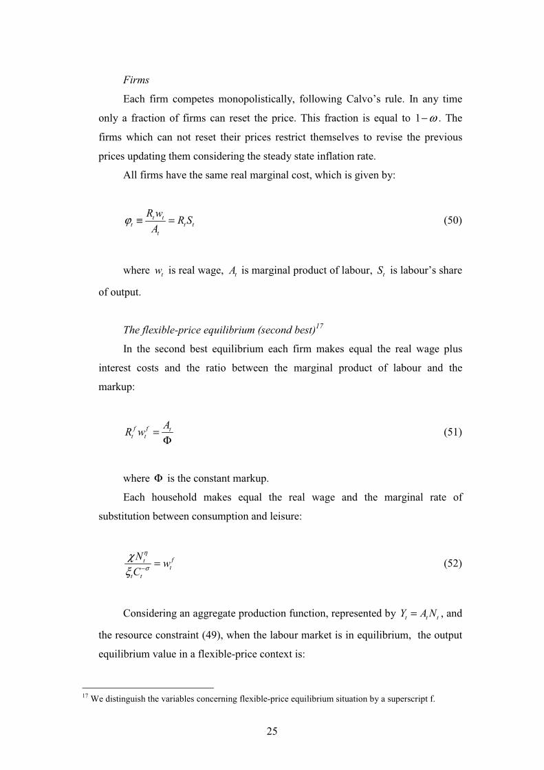
All firms have the same real marginal cost, which is given by:
t tt t t
t
R wR S
Aϕ ≡ = (50)
where tw is real wage, tA is marginal product of labour, tS is labour’s share
of output.
The flexible-price equilibrium (second best)17
In the second best equilibrium each firm makes equal the real wage plus
interest costs and the ratio between the marginal product of labour and the
markup:
f f tt t
AR w =
Φ (51)
where Φ is the constant markup.
Each household makes equal the real wage and the marginal rate of
substitution between consumption and leisure:
ftt
t t
Nw
C
η
σ
χ
ξ −= (52)
Considering an aggregate production function, represented by t t tY A N= , and
the resource constraint (49), when the labour market is in equilibrium, the output
equilibrium value in a flexible-price context is:
17
We distinguish the variables concerning flexible-price equilibrium situation by a superscript f.
26
( )1/1
f t t tt f
t
AY
R
σ ησ ηξ γ
χ
+− +
= Φ
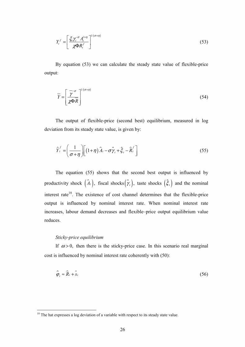
(53)
By equation (53) we can calculate the steady state value of flexible-price
output:
( )1/
YR
σ ησγ
χ
+− =
Φ (54)
The output of flexible-price (second best) equilibrium, measured in log
deviation from its steady state value, is given by:
( ) 11
f f
t t tt tY A Rη σ γ ξσ η
= + − + − + (55)
The equation (55) shows that the second best output is influenced by
productivity shock ( ) ,tA fiscal shocks ( ) ,tγ taste shocks ( )tξ and the nominal
interest rate18
. The existence of cost channel determines that the flexible-price
output is influenced by nominal interest rate. When nominal interest rate
increases, labour demand decreases and flexible–price output equilibrium value
reduces.
Sticky-price equilibrium
If 0,ω > then there is the sticky-price case. In this scenario real marginal
cost is influenced by nominal interest rate coherently with (50):
t tt R sϕ ≈ + (56)
18
The hat expresses a log deviation of a variable with respect to its steady state value.
27
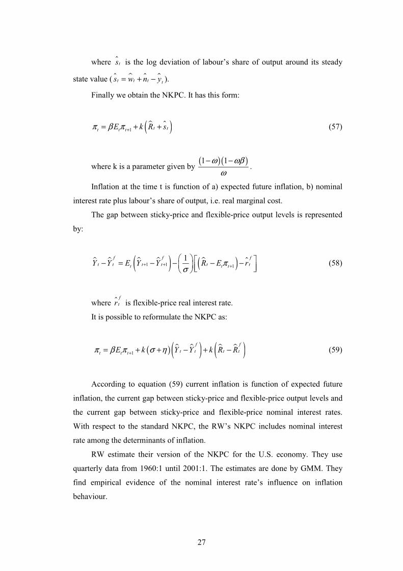
where ts is the log deviation of labour’s share of output around its steady
state value ( t t t ts w n y= + − ).
Finally we obtain the NKPC. It has this form:
( )1 t tt t tE k R sπ β π += + + (57)
where k is a parameter given by ( )( )1 1ω ωβ
ω
− −.
Inflation at the time t is function of a) expected future inflation, b) nominal
interest rate plus labour’s share of output, i.e. real marginal cost.
The gap between sticky-price and flexible-price output levels is represented
by:
( ) ( )1 1 1
1f f f
t t t t t tt t tY Y E Y Y R E rπσ
+ + +
− = − − − − (58)
where f
tr is flexible-price real interest rate.
It is possible to reformulate the NKPC as:
( ) ( ) ( )1
f f
t t t tt t tE k Y Y k R Rπ β π σ η+= + + − + − (59)
According to equation (59) current inflation is function of expected future
inflation, the current gap between sticky-price and flexible-price output levels and
the current gap between sticky-price and flexible-price nominal interest rates.
With respect to the standard NKPC, the RW’s NKPC includes nominal interest
rate among the determinants of inflation.
RW estimate their version of the NKPC for the U.S. economy. They use
quarterly data from 1960:1 until 2001:1. The estimates are done by GMM. They
find empirical evidence of the nominal interest rate’s influence on inflation
behaviour.
28
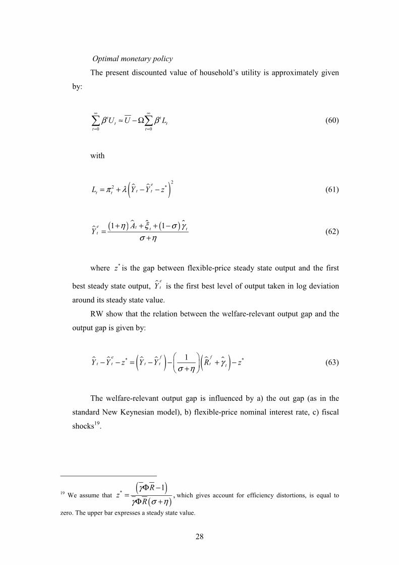
Optimal monetary policy
The present discounted value of household’s utility is approximately given
by:
0 0
t t
t t
t t
U U Lβ β∞ ∞
= =
≈ − Ω (60)
with
( )2
2 *e
t tt tL Y Y zπ λ= + − − (61)
( ) ( ) 1 1e t t tt
AY
η ξ σ γ
σ η
+ + + −=
+ (62)
where *z is the gap between flexible-price steady state output and the first
best steady state output, e
tY is the first best level of output taken in log deviation
around its steady state value.
RW show that the relation between the welfare-relevant output gap and the
output gap is given by:
( ) ( )* *1e f f
t t t t t tY Y z Y Y R zγσ η
− − = − − + − +
(63)
The welfare-relevant output gap is influenced by a) the out gap (as in the
standard New Keynesian model), b) flexible-price nominal interest rate, c) fiscal
shocks19
.
19 We assume that
( )( )
*1
,R
zR
γ
γ σ η
Φ −=
Φ +which gives account for efficiency distortions, is equal to
zero. The upper bar expresses a steady state value.
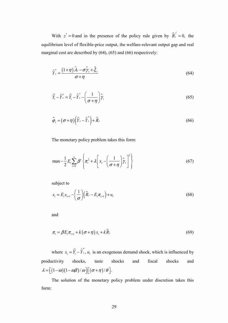
29
With * 0z = and in the presence of the policy rule given by 0,f
tR = the
equilibrium level of flexible-price output, the welfare-relevant output gap and real
marginal cost are described by (64), (65) and (66) respectively:
( ) * 1 t t tt
AY
η σ γ ξ
σ η
+ − +=
+ (64)
* 1e
t t tt tY Y Y Y γσ η
− = − − +
(65)
( ) ( ) *
t t tt Y Y Rϕ σ η= + − + (66)
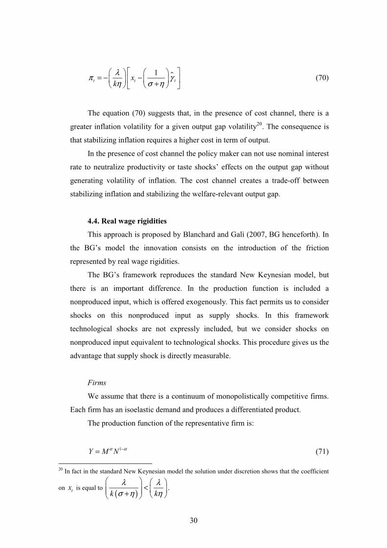
The monetary policy problem takes this form:
2
2
0
1 1max
2
t
tt t t
t
E xβ π λ γσ η
∞
=
− + − +
(67)
subject to
( )1 1
1tt t t t t tx E x R E uπ
σ+ +
= − − +
(68)
and
( ) 1 tt t t tE k x k Rπ β π σ η+= + + + (69)
where *
,tt tx Y Y= − tu is an exogenous demand shock, which is influenced by
productivity shocks, taste shocks and fiscal shocks and
( ) ( ) ( )1 1 / / .λ ω ωβ ω σ η θ= − − +
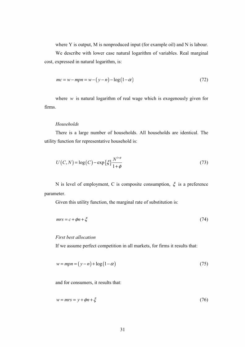
The solution of the monetary policy problem under discretion takes this
form:
30
1tt tx
k
λπ γ
η σ η
= − − +
(70)
The equation (70) suggests that, in the presence of cost channel, there is a
greater inflation volatility for a given output gap volatility20
. The consequence is
that stabilizing inflation requires a higher cost in term of output.
In the presence of cost channel the policy maker can not use nominal interest
rate to neutralize productivity or taste shocks’ effects on the output gap without
generating volatility of inflation. The cost channel creates a trade-off between
stabilizing inflation and stabilizing the welfare-relevant output gap.
4.4. Real wage rigidities
This approach is proposed by Blanchard and Galì (2007, BG henceforth). In
the BG’s model the innovation consists on the introduction of the friction
represented by real wage rigidities.
The BG’s framework reproduces the standard New Keynesian model, but
there is an important difference. In the production function is included a
nonproduced input, which is offered exogenously. This fact permits us to consider
shocks on this nonproduced input as supply shocks. In this framework
technological shocks are not expressly included, but we consider shocks on
nonproduced input equivalent to technological shocks. This procedure gives us the
advantage that supply shock is directly measurable.
Firms
We assume that there is a continuum of monopolistically competitive firms.
Each firm has an isoelastic demand and produces a differentiated product.
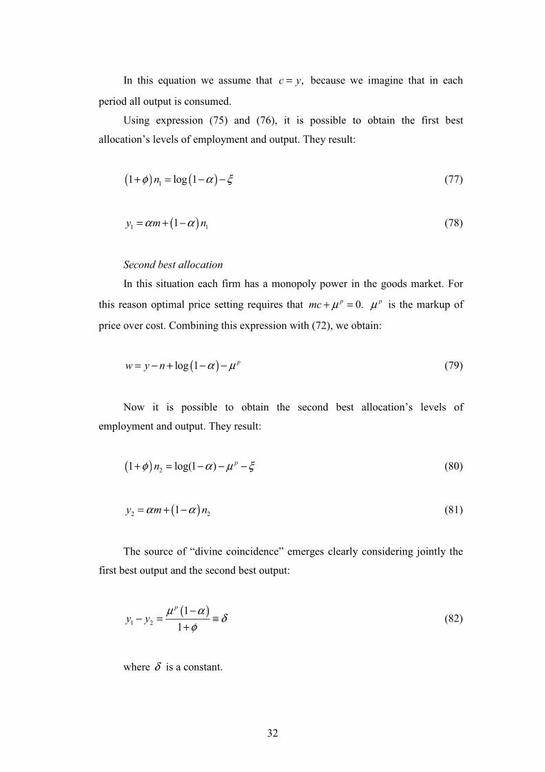
The production function of the representative firm is:
1Y M Nα α−= (71)
20
In fact in the standard New Keynesian model the solution under discretion shows that the coefficient
on tx is equal to ( )
.k k
λ λ
σ η η
< +
31
where Y is output, M is nonproduced input (for example oil) and N is labour.
We describe with lower case natural logarithm of variables. Real marginal
cost, expressed in natural logarithm, is:
( ) ( )log 1mc w mpn w y n α= − = − − − − (72)
where w is natural logarithm of real wage which is exogenously given for
firms.
Households
There is a large number of households. All households are identical. The
utility function for representative household is:
( ) ( ) 1
, log exp1
NU C N C
φ
ξφ
+
= −+
(73)
N is level of employment, C is composite consumption, ξ is a preference
parameter.
Given this utility function, the marginal rate of substitution is:
mrs c nφ ξ= + + (74)
First best allocation
If we assume perfect competition in all markets, for firms it results that:
( ) ( )log 1w mpn y n α= = − + − (75)
and for consumers, it results that:
w mrs y nφ ξ= = + + (76)
32
In this equation we assume that ,c y= because we imagine that in each
period all output is consumed.
Using expression (75) and (76), it is possible to obtain the first best
allocation’s levels of employment and output. They result:
( ) ( )11 log 1nφ α ξ+ = − − (77)
( )1 11y m nα α= + − (78)
Second best allocation
In this situation each firm has a monopoly power in the goods market. For
this reason optimal price setting requires that 0.pmc µ+ = pµ is the markup of
price over cost. Combining this expression with (72), we obtain:
( )log 1 pw y n α µ= − + − − (79)
Now it is possible to obtain the second best allocation’s levels of
employment and output. They result:
( ) 21 log(1 ) pnφ α µ ξ+ = − − − (80)
( )2 21y m nα α= + − (81)
The source of “divine coincidence” emerges clearly considering jointly the
first best output and the second best output:
( )1 2
1
1
p
y yµ α
δφ
−− = ≡
+ (82)
where δ is a constant.
33
Even though the levels of the first best and the second best output change
over time, the gap between them results always constant.
Real wage rigidities
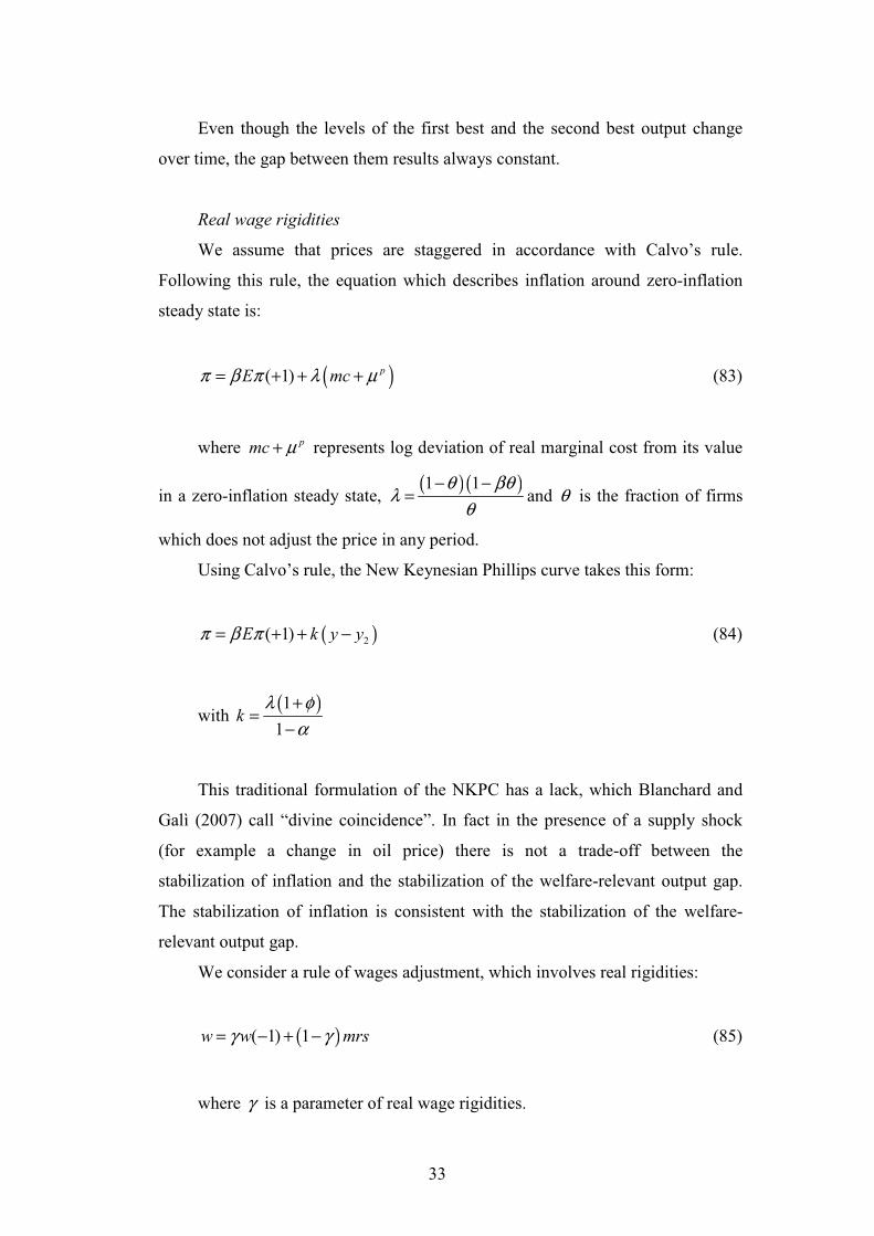
We assume that prices are staggered in accordance with Calvo’s rule.
Following this rule, the equation which describes inflation around zero-inflation
steady state is:
( )( 1) pE mcπ β π λ µ= + + + (83)
where pmc µ+ represents log deviation of real marginal cost from its value
in a zero-inflation steady state, ( )( )1 1θ βθ
λθ
− −= and θ is the fraction of firms
which does not adjust the price in any period.
Using Calvo’s rule, the New Keynesian Phillips curve takes this form:
( )2( 1)E k y yπ β π= + + − (84)
with ( )1
1k
λ φ
α
+=
−
This traditional formulation of the NKPC has a lack, which Blanchard and
Galì (2007) call “divine coincidence”. In fact in the presence of a supply shock
(for example a change in oil price) there is not a trade-off between the
stabilization of inflation and the stabilization of the welfare-relevant output gap.
The stabilization of inflation is consistent with the stabilization of the welfare-
relevant output gap.
We consider a rule of wages adjustment, which involves real rigidities:
( )( 1) 1w w mrsγ γ= − + − (85)
where γ is a parameter of real wage rigidities.
34
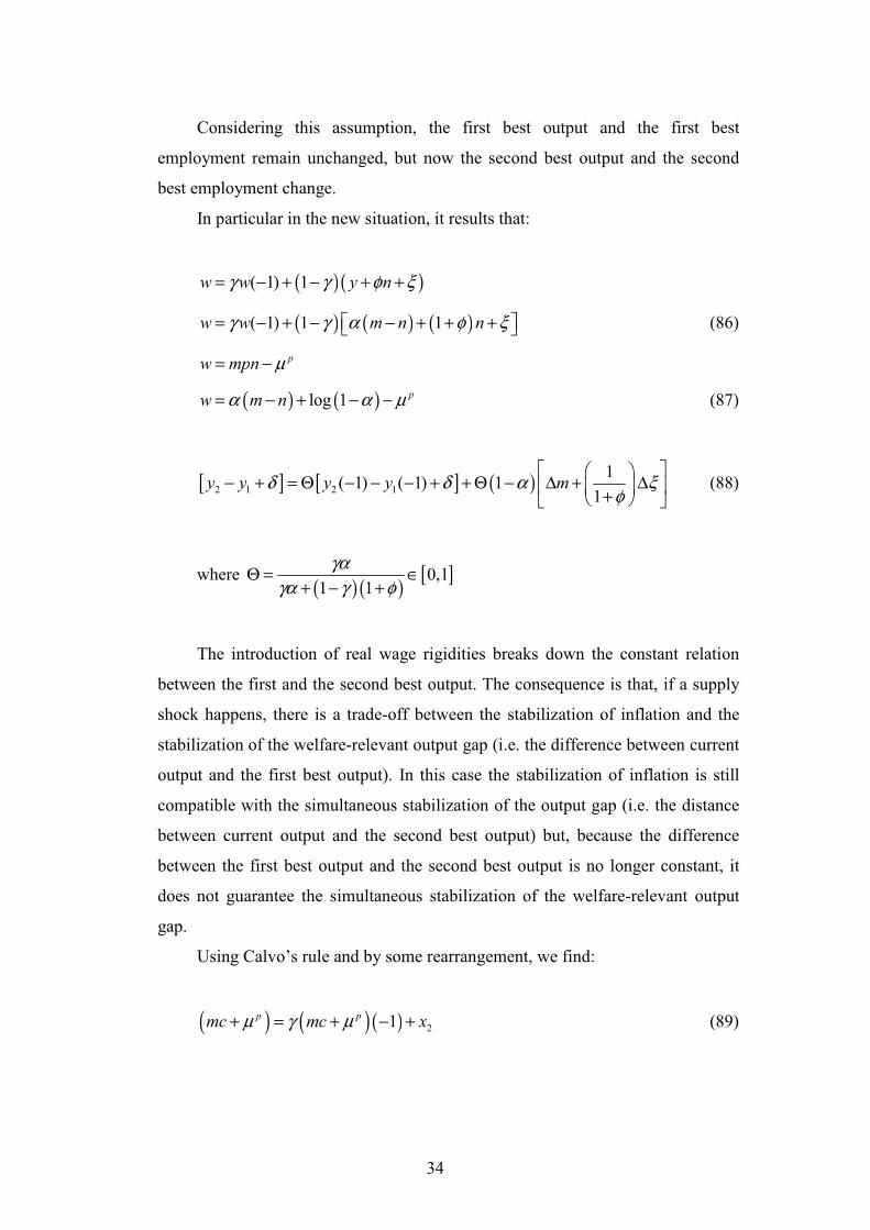
Considering this assumption, the first best output and the first best
employment remain unchanged, but now the second best output and the second
best employment change.
In particular in the new situation, it results that:
( )( )( 1) 1w w y nγ γ φ ξ= − + − + +
( ) ( ) ( )( 1) 1 1w w m n nγ γ α φ ξ= − + − − + + + (86)
pw mpn µ= −
( ) ( )log 1 pw m nα α µ= − + − − (87)
[ ] [ ] ( )2 1 2 1
1( 1) ( 1) 1
1y y y y mδ δ α ξ
φ
− + = Θ − − − + + Θ − ∆ + ∆ +
(88)
where ( ) ( )
[ ]0,11 1
γα
γα γ φΘ = ∈
+ − +
The introduction of real wage rigidities breaks down the constant relation
between the first and the second best output. The consequence is that, if a supply
shock happens, there is a trade-off between the stabilization of inflation and the
stabilization of the welfare-relevant output gap (i.e. the difference between current
output and the first best output). In this case the stabilization of inflation is still
compatible with the simultaneous stabilization of the output gap (i.e. the distance
between current output and the second best output) but, because the difference
between the first best output and the second best output is no longer constant, it
does not guarantee the simultaneous stabilization of the welfare-relevant output
gap.
Using Calvo’s rule and by some rearrangement, we find:
( ) ( )( ) 21p pmc mc xµ γ µ+ = + − + (89)
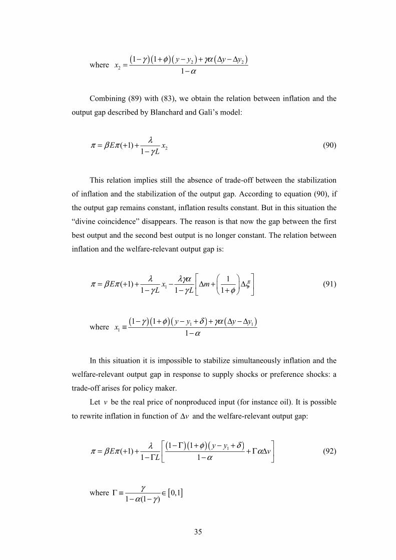
35
where ( ) ( )( ) ( )2 2
2
1 1
1
y y y yx
γ φ γα
α
− + − + ∆ − ∆=
−
Combining (89) with (83), we obtain the relation between inflation and the
output gap described by Blanchard and Galì’s model:
2( 1)1
E xL
λπ β π
γ= + +
− (90)
This relation implies still the absence of trade-off between the stabilization
of inflation and the stabilization of the output gap. According to equation (90), if
the output gap remains constant, inflation results constant. But in this situation the
“divine coincidence” disappears. The reason is that now the gap between the first
best output and the second best output is no longer constant. The relation between
inflation and the welfare-relevant output gap is:
1
1( 1)
1 1 1E x m
L L
λ λγαπ β π ξ
γ γ φ
= + + − ∆ + ∆ − − +
(91)
where ( ) ( )( ) ( )1 1
1
1 1
1
y y y yx
γ φ δ γα
α
− + − + + ∆ − ∆≡
−
In this situation it is impossible to stabilize simultaneously inflation and the
welfare-relevant output gap in response to supply shocks or preference shocks: a
trade-off arises for policy maker.
Let v be the real price of nonproduced input (for instance oil). It is possible
to rewrite inflation in function of v∆ and the welfare-relevant output gap:
( ) ( )( )11 1( 1)
1 1
y yE v
L
φ δλπ β π α
α
− Γ + − + = + + + Γ ∆
− Γ − (92)
where [ ]0,11 (1 )
γ
α γΓ ≡ ∈
− −
36
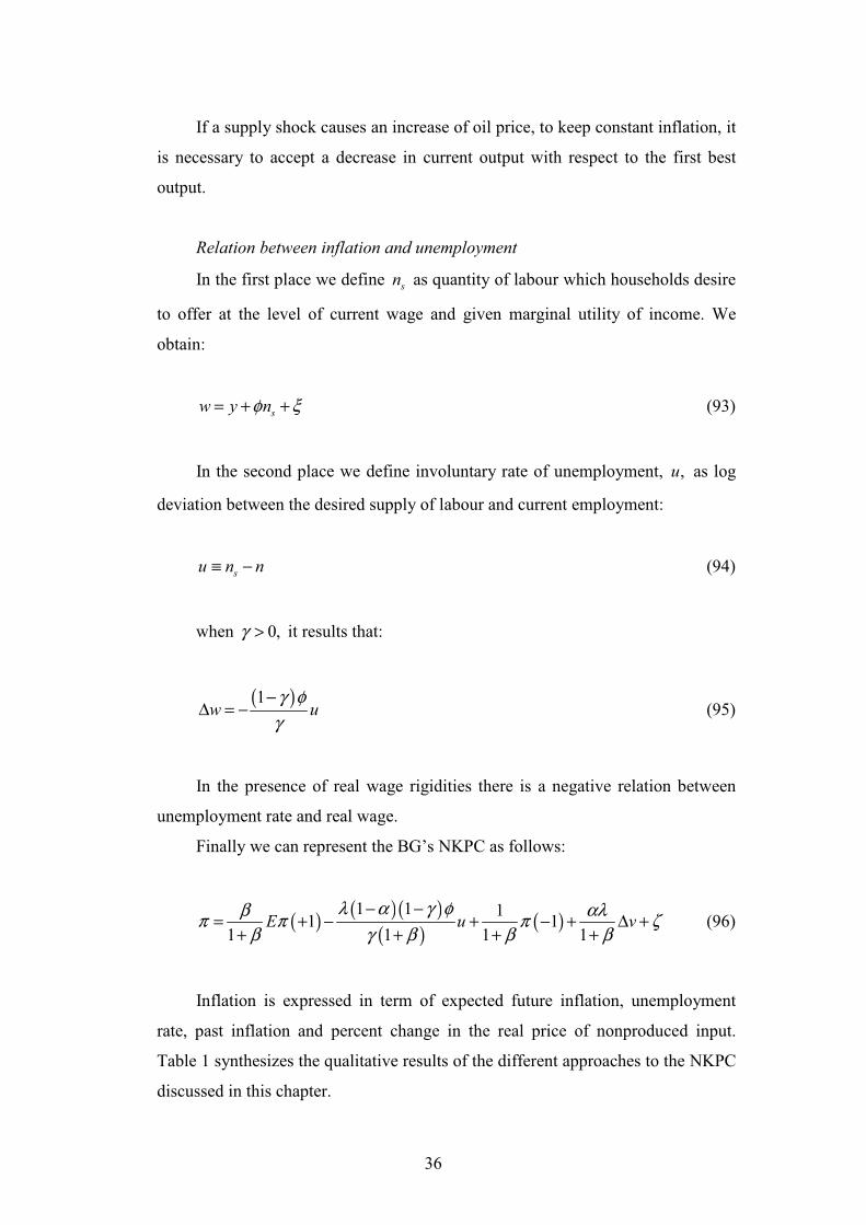
If a supply shock causes an increase of oil price, to keep constant inflation, it
is necessary to accept a decrease in current output with respect to the first best
output.
Relation between inflation and unemployment
In the first place we define sn as quantity of labour which households desire
to offer at the level of current wage and given marginal utility of income. We
obtain:
sw y nφ ξ= + + (93)
In the second place we define involuntary rate of unemployment, ,u as log
deviation between the desired supply of labour and current employment:
su n n≡ − (94)
when 0,γ > it results that:
( )1w u
γ φ
γ
−∆ = − (95)
In the presence of real wage rigidities there is a negative relation between
unemployment rate and real wage.
Finally we can represent the BG’s NKPC as follows:
( )( )( )
( )( )
1 1 11 1
1 1 1 1E u v
λ α γ φβ αλπ π π ζ
β γ β β β
− −= + − + − + ∆ +
+ + + + (96)
Inflation is expressed in term of expected future inflation, unemployment
rate, past inflation and percent change in the real price of nonproduced input.
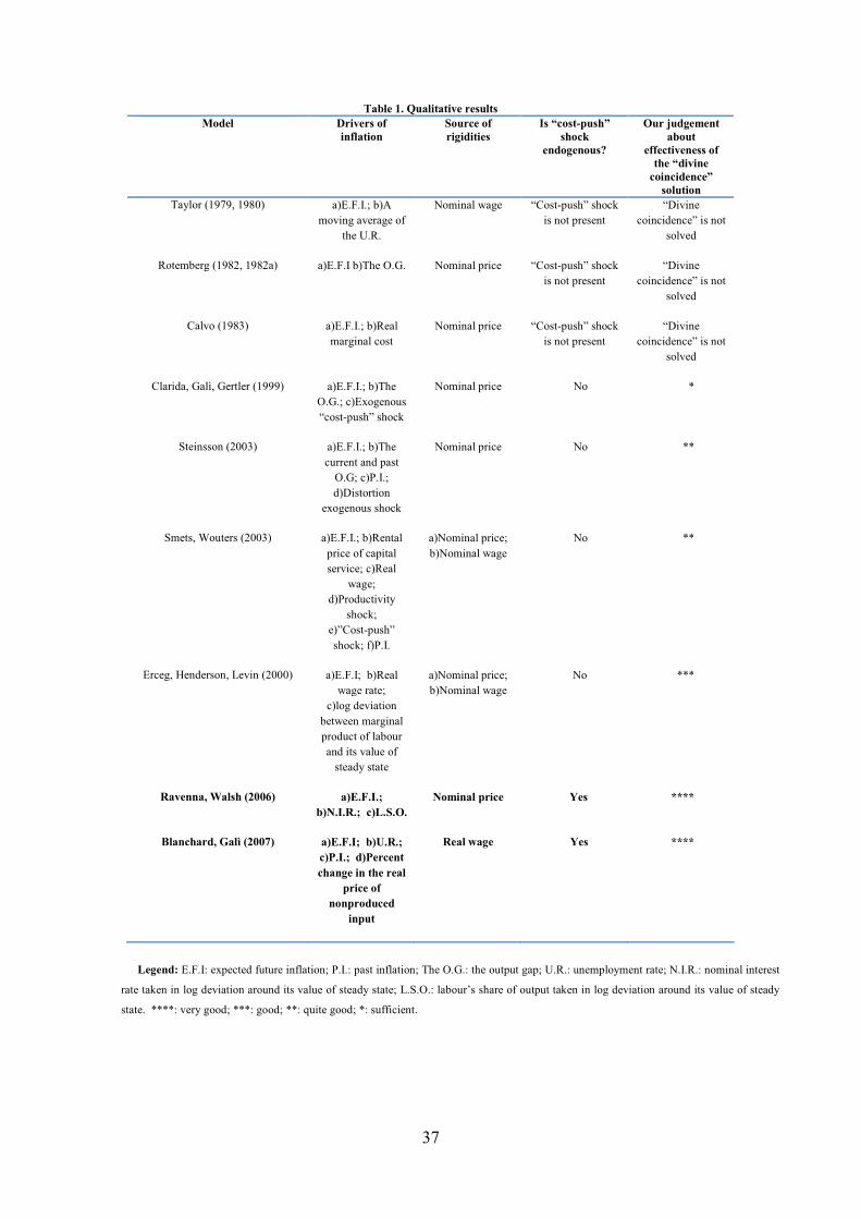
Table 1 synthesizes the qualitative results of the different approaches to the NKPC
discussed in this chapter.
37
Table 1. Qualitative results
Model Drivers of
inflation
Source of
rigidities
Is “cost-push”
shock
endogenous?
Our judgement
about
effectiveness of
the “divine
coincidence”
solution
Taylor (1979, 1980) a)E.F.I.; b)A
moving average of
the U.R.
Nominal wage “Cost-push” shock
is not present
“Divine
coincidence” is not
solved
Rotemberg (1982, 1982a) a)E.F.I b)The O.G. Nominal price “Cost-push” shock
is not present
“Divine
coincidence” is not
solved
Calvo (1983) a)E.F.I.; b)Real
marginal cost
Nominal price “Cost-push” shock
is not present
“Divine
coincidence” is not
solved
Clarida, Galì, Gertler (1999) a)E.F.I.; b)The
O.G.; c)Exogenous
“cost-push” shock
Nominal price No *
Steinsson (2003) a)E.F.I.; b)The
current and past
O.G; c)P.I.;
d)Distortion
exogenous shock
Nominal price No **
Smets, Wouters (2003) a)E.F.I.; b)Rental
price of capital
service; c)Real
wage;
d)Productivity
shock;
e)”Cost-push”
shock; f)P.I.
a)Nominal price;
b)Nominal wage
No **
Erceg, Henderson, Levin (2000) a)E.F.I; b)Real
wage rate;
c)log deviation
between marginal
product of labour
and its value of
steady state
a)Nominal price;
b)Nominal wage
No ***
Ravenna, Walsh (2006) a)E.F.I.;
b)N.I.R.; c)L.S.O.
Nominal price Yes ****
Blanchard, Galì (2007) a)E.F.I; b)U.R.;
c)P.I.; d)Percent
change in the real
price of
nonproduced
input
Real wage Yes ****
Legend: E.F.I: expected future inflation; P.I.: past inflation; The O.G.: the output gap; U.R.: unemployment rate; N.I.R.: nominal interest
rate taken in log deviation around its value of steady state; L.S.O.: labour’s share of output taken in log deviation around its value of steady
state. ****: very good; ***: good; **: quite good; *: sufficient.
38
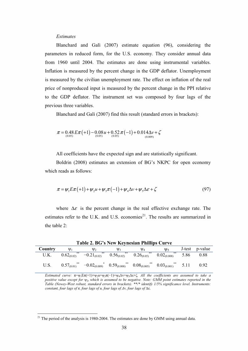
Estimates
Blanchard and Galì (2007) estimate equation (96), considering the
parameters in reduced form, for the U.S. economy. They consider annual data
from 1960 until 2004. The estimates are done using instrumental variables.
Inflation is measured by the percent change in the GDP deflator. Unemployment
is measured by the civilian unemployment rate. The effect on inflation of the real
price of nonproduced input is measured by the percent change in the PPI relative
to the GDP deflator. The instrument set was composed by four lags of the
previous three variables.
Blanchard and Galì (2007) find this result (standard errors in brackets):
( ) ( )(0.05) (0.05) (0.05) (0.009)
0.48 1 0.08 0.52 1 0.014E u vπ π π ζ= + − + − + ∆ +
All coefficients have the expected sign and are statistically significant.
Boldrin (2008) estimates an extension of BG’s NKPC for open economy
which reads as follows:
( ) ( )1 2 3 4 51 1E u vπ ψ π ψ ψ π ψ ψ ε ζ= + + + − + ∆ + ∆ + (97)
where ε∆ is the percent change in the real effective exchange rate. The
estimates refer to the U.K. and U.S. economies21
. The results are summarized in
the table 2:
Table 2. BG’s New Keynesian Phillips Curve
Country 1 2 3 4 5 J-test p-value
U.K. 0.62(0.02)**
−0.21(0.02)**
0.56(0.02)**
0.26(0.05)**
0.02(0.008)**
5.86 0.88
U.S. 0.57(0.01)**
−0.02(0.009)*
0.59(0.008)**
0.08(0.005)**
0.03(0.001)**
5.11 0.92
Estimated curve: =1E(+1)+2u+3(−1)+4v+5+. All the coefficients are assumed to take a
positive value except for 2, which is assumed to be negative. Note: GMM point estimates reported in the
Table (Newey-West robust, standard errors in brackets). **/* identify 1/5% significance level. Instruments:
constant, four lags of , four lags of u, four lags of v, four lags of .
21
The period of the analysis is 1980-2004. The estimates are done by GMM using annual data.
39
These estimates show that the BG’s NKPC fit the data well. In particular all
coefficients have the expected sign and are statistically significant.
5. Future developments and new challenges
In the recent years the economic literature involving the New Keynesian
model in general and the NKPC in particular is growing in a massive way. In fact
today it is possible to identify the New Keynesian model as the main tool to
analyse the short-run fluctuations of the economy. The quick growth of the New
Keynesian paradigm has been generated by the continuous progresses realized in
the past two decades. Although these improvements, to reach a more satisfactory
level of the reality’s comprehension, it is essential to tackle some problematic
aspects which have not had still a response.
In particular this survey has analysed a specific problem afflicting the
NKPC, known in the economic literature as “divine coincidence”, and the
solutions proposed to it currently. The specifications of the NKPC, which are
arisen by the solutions proposed, will have to be checked in the future analyses to
understand their degree of validity. Nevertheless it seems obvious that the
complexity of the problem, because of its links with a multiplicity of variables,
will require further energies to develop the research along different straights22
:
1) The specifications of the NKPC, addressed to solve the “divine
coincidence”, are hybrid in the sense that inflation is explained by both
past inflation and expected future inflation. Many economists have tried
to quantify the relative importance of these variables in influencing
inflation dynamics. Currently there is not a large consensus about what
is predominant between these two variables. It is possible to highlight
two different positions in this subject. The first is represented by Galì
and Gertler (1999) and Galì, Gertler and López-Salido (2005).
According to these authors the expected forward-looking component is
preponderant in explaining inflation. The second is expressed by Rudd
and Whelan (2006, 2007). These authors doubt that existing empirical
researches show a prevalence of expected future inflation in explaining
inflation behaviour.
22
The points 3), 4) and 5) have been clearly expressed by Galì and Gertler (2007) and Galì (2008).
40
2) In the empirical analyses of the NKPC in general and with particular
attention to the specifications used to solve the “divine coincidence”, a
relevant problem is the choice of the variable which expresses the real
marginal cost (which in general is proxied by the output gap). The
failure of the New Keynesian Phillips curve in fitting the data when the
excess of demand is represented by the log of the detrended real GDP
induces many authors to criticize this variable because of its inadequacy
as proxy to real marginal cost (i.e. the variable which theoretically drives
inflation in the NKPC). For this reason Galì and Gertler (1999) and
Sbordone (2002) propose to use labour’s share of income as proxy of
real marginal cost. This choice is brought into question by Rudd and
Whelan (2006, 2007). These economists elaborate an empirical estimate
using labour’s share of income as proxy of real marginal cost, and find a
weakness of the NKPC in fitting the data when it is estimated in this
way.
3) Rigidities can be introduced in the New Keynesian model following two
methods23
: i) time-dependent models; ii) state-dependent models24
. The
solution more used is i). All the models analysed in this survey belong to
the time-dependent approach. In this approach (for example the Calvo’s
model) firms adjust their prices according to a fixed frequency.
Differently in the state-dependent approach firms adjust their prices
when certain variables (for examples costs) achieve some values. In this
way the rules of price adjustment become endogenous. Recent analyses
inspired by state-dependent approach are led by Dotsey, King and
Wolman (1999), Gertler and Leahy (2006), Midrigan (2006) and
Golosov and Lucas (2007).
4) The standard New Keynesian model and the implied NKPC suppose a
neoclassical labour market in which the workers modify their hours
worked but there is not involuntary unemployment. Many researchers try
to introduce in the New Keynesian model some frictions of the labour
market traditionally analysed in the matching and search literature. This
23
This classification is proposed by Ball, Mankiw and Romer (1988). 24
Probably the first formalization of the state-dependent approach is developed by Caplin and Spulber
(1987).
41
procedure can improve the comprehension of the reality in order to a
fundamental aspect as labour market’s dynamics. Some attempts along
this line are proposed by Walsh (2005), Trigari (2005), Blanchard and
Galì (2006) and Gertler, Sala and Trigari (2007).
5) A fundamental hypothesis of the New Keynesian model is that the
financial markets are perfectly competitive markets. Today a growing
number of economists tries to remove this assumption to create a model
which considers the imperfections which characterize the real financial
markets. This procedure offers the opportunity to inquiry more deeply
the role played by the monetary policy on the short-run fluctuations.
This kind of analysis can improve the comprehension of inflation
dynamics involved by the NKPC. This line of research has been
followed by Bernanke, Gertler and Gilchrist (1999), Gilchrist and Leahy
(2002), Christiano, Motto and Rostagno (2006), Faia and Monacelli
(2006), Monacelli (2006), Iacoviello (2006).
6. Conclusions
This chapter discusses a fundamental part of the New Keynesian model, the
so-called NKPC. We analyse the theoretical bases of the NKPC and emphasize
that the standard explanation of inflation behaviour in the New Keynesian
framework has a shortcoming. This lack is called by Blanchard and Galì (2007)
“divine coincidence”, i.e. the absence of a trade-off between stabilizing inflation
and stabilizing the welfare-relevant output gap, when a shock hits the economy.
We identify in the economic literature four solutions to this problem. The
solutions which are proposed have in common the attempt of representing some
form of “cost-push” shock to generate a trade-off between the stabilization of
inflation and the stabilization of the welfare-relevant output gap.
In particular two solutions among the others seem to us particularly
efficacious in tackling the “divine coincidence” problem. The two theoretical
analyses are proposed by Blanchard and Galì (2007) and Ravenna and Walsh
(2006). Both are able to generate a “cost-push” shock endogenously. But the
difference between them consists of the source which nourishes this “cost-push”
shock. In the Blanchard and Galì’s work the source of the “cost-push” shock is

42
represented by real wage rigidities, in the Ravenna and Walsh’s model by the cost
channel.
43
References
Ball L., Mankiw. N.G., Romer D. (1988), “The New Keynesian Economics
and the Output-Inflation Trade-off,” Brookings Papers on Economic Activity, 1,
pp. 1-65.
Bernanke B., Gertler M., Gilchrist S. (1999), “The Financial Accelerator
in a Quantitative Business Cycle Framework,“ in the Handbook of
Macroeconomics, vol. 1C, ed. John Taylor and Michael Woodford, chapter 21,
North-Holland.
Blanchard O., Galì J. (2006), “A New Keynesian Model with
Unemployment,” MIT, Department of Economics Working Paper No. 06-22.
Blanchard O., Galì J. (2007), “Real Wage Rigidities and the New
Keynesian Model,” Journal of Money, Credit and Banking, Supplement to vol.
39(1), pp. 35-65.
Boldrin N. (2008), “Assessing the Relevance of Oil and Exchange Rates in
the New Keynesian Phillips Curve,” mimeo.
Calvo G. (1983), “Staggered Prices in a Utility-Maximizing Framework,”
Journal of Monetary Economics, 12(3), pp. 383-398.
Campbell J., Mankiw N.G. (1989), “Consumption, Income, and Interest
Rates: Reinterpreting the Time Series Evidence,” NBER Macroeconomics Annual
1989, pp. 185-216.
Caplin A., Spulber D. (1987), “Menu Costs and the Neutrality of Money,”
Quarterly Journal of Economics, 102(4), pp. 703-725.
Christiano L., Motto R., Rostagno M. (2006), “Monetary Policy and Stock
Market Boom-Bust Cycles,” mimeo.
Clarida R., Galì J., Gertler M. (1999), “The Science of Monetary Policy:
A New Keynesian Perspective,” Journal of Economic Literature, vol. 37(4), pp.
1661-1707.
Clarida R., Galì J., Gertler M. (2001), “Optimal Monetary Policy in Open
vs. Closed Economies: An Integrated Approach,” American Economic Review,
vol. 91(2), pp. 248-252.
Dotsey M., King R., Wolman A. (1999), “State Dependent Pricing and the
General Equilibrium Dynamics of Money and Output,” Quarterly Journal of
Economics, 114(2), pp. 655-690.
44
Erceg C., Henderson D., Levin A. (2000), “Optimal Monetary Policy with
Staggered Wage and Price Contracts,” Journal of Monetary Economics. 46(2), pp.
281-313.
Faia E., Monacelli T. (2006), “Optimal Interest Rate Rules, Asset Prices
and Credit Frictions,” Journal of Economic Dynamics and Control, vol. 31(10),
pp. 3228-3254.
Fischer S. (1977), “Long-Term Contracts, Rational Expectations, and the
Optimal Money Supply Rule,” Journal of Political Economy, vol. 85(1), pp. 191-
205.
Fuhrer J., Moore G. (1995), “Inflation Persistence,” Quarterly Journal of
Economics, 440, pp. 127-159.
Fuhrer J. (1997), “The (Un)Importance of Forward-Looking Behavior in
Price Specifications,” Journal of Money, Credit and Banking, 29(3), pp. 338-350.
Galì J. (2008), “The New Keynesian Approach to Monetary Policy
Analysis: Lessons and New Directions,” mimeo.
Galì J., Gertler M. (1999), “Inflation Dynamics: A Structural Econometric
Analysis,” Journal of Monetary Economics, vol. 44(2), pp. 195-222.
Galì J., Gertler M. (2007), “Macroeconomic Modeling for Monetary Policy
Evaluation,” Journal of Economic Perspectives, vol. 21(4), pp. 25-45.
Galì J., Gertler M., López-Salido D. (2005), “Robustness of the Estimates
of the Hybrid New Keynesian Phillips Curve,” Journal of Monetary Economics,
52(6), pp. 1107-1118.
Gertler M., Leahy J. (2006), “A Phillips Curve with an S-s Foundation,”
Federal Reserve Bank of Philadelphia, Working Paper 06-8.
Gertler M., Sala L., Trigari A. (2007), “An Estimated Monetary DSGE
Model with Unemployment and Staggered Nash Wage Bargaining,” Unpublished
paper.
Gilchrist S., Leahy J. (2002), “Monetary Policy and Asset Prices,” Journal
of Monetary Economics, 49(1), pp. 75-97.
Golosov M., Lucas R. (2007), “Menu Costs and Phillips Curves,” Journal
of Political Economy, 115(2), pp. 171-199.
Goodfriend M., King R. (1997), “The New Neoclassical Synthesis and the
Role of Monetary Policy,” NBER Macroeconomics Annual 1997, pp. 231-283.
45
Iacoviello M. (2006), “House Prices, Borrowing Constraints and Monetary
Policy in the Business Cycle,” American Economic Review, 95(3), pp. 739-764.
Ireland P. (1997), “A Small, Structural, Quarterly Model for Monetary
Policy Evaluation,” Carnegie-Rochester Conference Series on Public Policy, vol.
47, pp. 83-108.
King R., Wolman A. (1999), “What Should the Monetary Authority Do
when Prices Are Sticky?,” in Monetary Policy Rules, J. Taylor (ed.), The
University of Chicago Press, Chicago, pp. 349-398.
Lucas R. (1976), “Econometric Policy Evaluation: A Critique,” Carnegie-
Rochester Conference Series on Public Policy, vol. 1, pp. 19-46.
Midrigan V. (2007), “Menu Costs, Multi-Product Firms, and Aggregate
Fluctuations,” CFS Working Paper Series 2007/13, Center for Financial Studies.
Monacelli T. (2007), “Optimal Monetary Policy with Collateralized
Household Debt and Borrowing Constraints,” in Asset Prices and Monetary
Policy, J. Campbell (ed.), University of Chicago Press.
Obstfeld M., Rogoff. K. (1996), Foundations of International
Macroeconomics, MIT Press, Cambridge, MA.
Phillips A.W. (1958), “The Relationship Between Unemployment and the
Rate of Change of Money Wage Rates in the UK, 1861-1957,” Economica.
Ravenna F. and Walsh C. (2006), “Optimal Monetary Policy with the Cost
Channel,” Journal of Monetary Economics, 53(2), pp. 199-216.
Roberts J. (1995), “New Keynesian Economics and the Phillips Curve,”
Journal of Money, Credit and Banking, vol. 27(4), pp. 975-984.
Roberts J. (2005), “How Well Does the New Keynesian Sticky-Price Model
Fit the Data?,” Contributions to Macroeconomics, vol. 5, pp. 1-37.
Rotemberg J. (1982), “Sticky Prices in the United States,” Journal of
Political Economy, vol. 90(6), pp. 1187-1211.
Rotemberg J. (1982a), “Monopolistic Price Adjustment and Aggregate
Output,” Review of Economic Studies, vol. 49(4), pp. 517-531.
Rotemberg J. (1987), “The New Keynesian Microfoundations,” NBER
Macroeconomics Annual 1987, pp. 69-104.
46
Rotemberg J., Woodford M. (1997), “An Optimization-Based Econometric
Framework for the Evaluation of Monetary Policy,” NBER Macroeconomics
Annual 1997, pp. 297-346.
Rotemberg J., Woodford M. (1999), “Interest Rate Rules in an Estimated
Sticky Price Model,” in Monetary Policy Rules, J. Taylor (ed.), University of
Chicago Press, Chicago, pp. 57-119.
Rudd J., Whelan K. (2006), “Can Rational Expectations Sticky-Price
Models Explain Inflation Dynamics?,” American Economic Review, 96(1), pp.
303-320.
Rudd J., Whelan K. (2007), “Modeling Inflation Dynamics: A Critical
Review of Recent Research,” Journal of Money, Credit and Banking, Supplement
to vol. 39(1), pp. 155-170.
Sbordone A. (2002), “Prices and Unit Labor Costs: A New Test of Price
Stickiness,” Journal of Monetary Economics, vol. 49(2), pp. 265-292.
Smets F., Wouters R. (2003), “An Estimated Dynamic Stochastic General
Equilibrium Model of the Euro Area,” Journal of the European Economic
Association, vol. 1(5), 1123-1175.
Steinsson J. (2003), “Optimal Monetary Policy in an Economy with
Inflation Persistence,” Journal of Monetary Economics, vol. 50(7), pp. 1425-1456.
Taylor J. (1979), “Staggered Wage Setting in a Macro Model,” American
Economic Review, vol. 69(2), pp. 108-113.
Taylor J. (1980), “Aggregate Dynamics and Staggered Contracts,“ Journal
of Political Economy, 88(1), pp. 1-23.
Trigari A. (2005), “Equilibrium Unemployment, Job Flows, and Inflation
Dynamics,” European Central Bank Working Paper 304.
Walsh C. (2005), “Labor Market Search, Sticky Prices, and Interest Rate
Rules,” Review of Economic Dynamics, 8(4), pp. 829-849.
Woodford M. (2003), Interest and Prices: Foundations of a Theory of
Monetary Policy, Princeton University Press.
Yun T. (1996), “Nominal Price Rigidity, Money Supply Endogeneity, and
Business Cycles,” Journal of Monetary Economics, 37(2), pp. 345-370.
47
CHAPTER 2
“Assessing the Relevance of Oil and Exchange Rates
in the New Keynesian Phillips Curve”
1. Introduction
In the modern macroeconomic literature the most popular framework for
analysing the monetary policy and business cycle is certainly the New Keynesian
model (Woodford 2003). An important ingredient of this model is the New
Keynesian Phillips curve, which may be represented as follows:
t=Ett+1+k(yt−yt*). In this formulation represents inflation, represents firms’
discount factor, Et identifies expectations taken at time t (i.e. with an information
set updated up to t), y is a measure of current GDP taken in logs, y* is the log of
the natural level of output, and (y−y*) is the “output gap”, i.e. the measure of
economic slack identifying the inflationary pressures coming due to aggregate
demand.
Many authors underline that the New Keynesian Phillips curve has a lack
(e.g. Mankiw (2001)). This lack consists in the absence of a trade-off between the
stabilization of inflation and the stabilization of the welfare-relevant output gap
(say, after a supply shock has hit the economy). The reason is that in this model
the wedge between the first and the second best output level is constant, then
when stabilizing output around the second best output level, monetary policy
makers also stabilize the first best output gap.1
Blanchard and Galì (2007) name this peculiarity of the standard New
Keynesian model “divine coincidence”. They also offer a rationale for the “divine
coincidence”: in the standard New Keynesian framework, no role is acknowledged
to non trivial real imperfections. Interestingly, they show that once real wage
rigidities are allowed to enter the model, the relationship between the first and the
second best output levels is not constant anymore. This implies the disappearance
of the “divine coincidence”, i.e. a meaningful inflation-output gap stabilization
trade-off arises. Notably, the Blanchard and Galì New Keynesian Phillips curve
(BGNKPC henceforth) also features the presence of the relative price of the
1 The second best output level is the one that would prevail under flexible prices in the presence of real
distortions such as monopolistic competition. By contrast, the first best output level is the one that
would realize under fully flexible prices and perfect competition in all markets.
48
nonproduced input (e.g. oil) as a regressor, so explicitly accounting for one of the
main sources of inflationary pressures in OECD countries.
This chapter estimates three different versions of the New Keynesian
Phillips curve for the United Kingdom and the United States of America in the
sample 1980-2004. Our empirical results point towards the likely misspecification
of the standard New Keynesian Phillips curve a la Woodford (2003). In fact, when
adding the producer price index (relative to the GDP deflator) and the growth rate
of the real effective exchange rate, these two regressors turn out to be largely
significant in both countries considered. Interestingly, the real effective exchange
rate helps corroborating the BGNKPC by i) capturing an otherwise missed source
of persistence (movements in the terms-of-trade) and ii) making unemployment
regressor’s sign significant and coherent with economic expectation.
This paper develops as follows. Section 2 offers a brief discussion of the
“divine coincidence” and presents the Blanchard-Galì proposal. Section 3
proposes the three different versions of the supply curve we take to the data. In
Section 4 we present our empirical findings, we compare the different abilities of
our competing models to fit the data and line up with an economist’s expectations
in terms of significance and sign of the included regressors. Section 5 concludes.
2. NKPC: standard model and Blanchard-Galì proposal
In the economic literature different solutions have been proposed to solve
the “divine coincidence”. A first approach is put forward by Clarida, Galì and
Gertler (1999). They add a “cost-push shock” in the New Keynesian Phillips curve.
In this way they create a trade-off between the stabilization of inflation and the
stabilization of the output gap. However, the so-called “cost-push” shock is a non-
micro-founded disturbance. Ideally, a model should endogenously generate a
time-varying wedge between the first and the second best level of output. In an
attempt to consider this criticism, Smets and Wouters (2003) and Clarida, Galì and
Gertler (2001) model “distortionary shocks” by allowing for variations in the
desired firms’ mark-up. Steinsson (2003) embeds variations in tax changes in an
otherwise standard model. In both scenarios the second best output is influenced
by distortionary shocks. Due to this reason, the relationship between the first and
the second best levels of output is not constant anymore, then monetary authorities
49
actually face the inflation-output volatility trade-off. Once more, the solution
relies on the manipulation of an exogenous autoregressive process, and it can not
be considered as being theoretically satisfactory.
A different approach to eliminate the “divine coincidence” is the one
proposed by Erceg, Henderson and Levin (2000). They show that, if both wages
and prices are staggered following Calvo’s rule, a meaningful gap arises. In Erceg,
Henderson and Levin’s model wage inflation and price inflation are influenced not
only by the output gap, but also by difference between current wage and the
second best level of wage. Consequence of this fact is that the “divine
coincidence” disappears either in price inflation or in wage inflation. However, it
is easy to show that in Erceg, Henderson and Levin’s model the stabilization of a
weighted average of wage and price inflation is compatible with the stabilization
of the welfare-relevant output gap. In fact, if we consider a composite inflation
rate =(wp+p
w)/(w+p), it is possible to rewrite the New Keynesian Phillips
curve in this way: =E(+1)+k(y−y2), where p is price inflation,
w is wage
inflation, k=[wp(1+)]/[(w+p)(1−)], is share of the nonproduced input in
production, represents the slope of the labour supply, w and p are coefficients
expressed in term of structural parameters. Then, the difference between the first
best level of output and the second best level of output is still constant, i.e.
y1−y2=2. Consequently the “divine coincidence” reappears.
A more theoretically appealing strategy to solve the problem of the “divine
coincidence” is proposed by Blanchard and Galì (2007). This approach is based on
the introduction of non trivial real imperfections in a New Keynesian model
featuring a CRS production function displaying labour and a nonproduced input (a
natural resource, e.g. oil). Following the lead by other authors (e.g. Hall (2005)),
Blanchard and Galì (2007) model real wage rigidities in order to create a gap
between desired labour supply and actual employment. Turning to the supply side,
the production function of the representative firm, which operates in monopolistic
competition, embeds an exogenously offered nonproduced input. They interpret
shocks to this nonproduced input as supply shocks, i.e. technological shocks. This
2 y1 represents the output that would realize under fully flexible prices and wages with perfect
competition in all markets; y2 stands for the natural output, i.e. the output that would obtain under both
flexible prices and wages in the presence of real distortion (for example monopolistic competition); is
a constant.
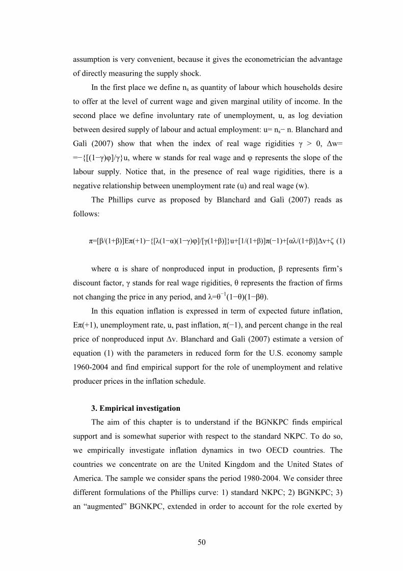
50
assumption is very convenient, because it gives the econometrician the advantage
of directly measuring the supply shock.
In the first place we define ns as quantity of labour which households desire
to offer at the level of current wage and given marginal utility of income. In the
second place we define involuntary rate of unemployment, u, as log deviation
between desired supply of labour and actual employment: u= ns− n. Blanchard and
Galì (2007) show that when the index of real wage rigidities > 0, w=
=−[(1−)]/u, where w stands for real wage and represents the slope of the
labour supply. Notice that, in the presence of real wage rigidities, there is a
negative relationship between unemployment rate (u) and real wage (w).
The Phillips curve as proposed by Blanchard and Galì (2007) reads as
follows:
=[/(1+)]E(+1)−[(1−)(1−)]/[(1+)]u+[1/(1+)](−1)+[/(1+)]v+ (1)
where is share of nonproduced input in production, represents firm’s
discount factor, stands for real wage rigidities, represents the fraction of firms
not changing the price in any period, and =−1
(1−)(1−).
In this equation inflation is expressed in term of expected future inflation,
E(+1), unemployment rate, u, past inflation, (−1), and percent change in the real
price of nonproduced input v. Blanchard and Galì (2007) estimate a version of
equation (1) with the parameters in reduced form for the U.S. economy sample
1960-2004 and find empirical support for the role of unemployment and relative
producer prices in the inflation schedule.
3. Empirical investigation
The aim of this chapter is to understand if the BGNKPC finds empirical
support and is somewhat superior with respect to the standard NKPC. To do so,
we empirically investigate inflation dynamics in two OECD countries. The
countries we concentrate on are the United Kingdom and the United States of
America. The sample we consider spans the period 1980-2004. We consider three
different formulations of the Phillips curve: 1) standard NKPC; 2) BGNKPC; 3)
an “augmented” BGNKPC, extended in order to account for the role exerted by
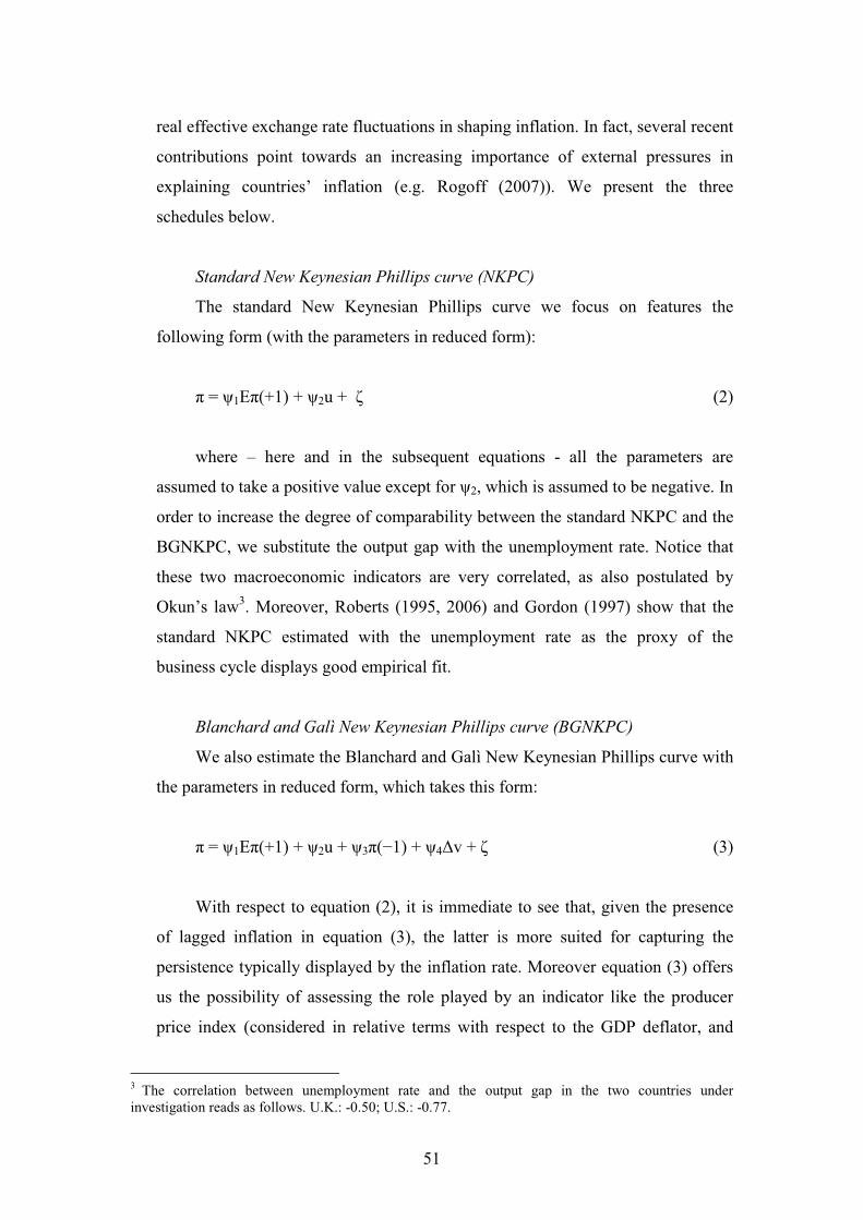
51
real effective exchange rate fluctuations in shaping inflation. In fact, several recent
contributions point towards an increasing importance of external pressures in
explaining countries’ inflation (e.g. Rogoff (2007)). We present the three
schedules below.
Standard New Keynesian Phillips curve (NKPC)
The standard New Keynesian Phillips curve we focus on features the
following form (with the parameters in reduced form):
= 1E(+1) + 2u + (2)
where – here and in the subsequent equations - all the parameters are
assumed to take a positive value except for 2, which is assumed to be negative. In
order to increase the degree of comparability between the standard NKPC and the
BGNKPC, we substitute the output gap with the unemployment rate. Notice that
these two macroeconomic indicators are very correlated, as also postulated by
Okun’s law3. Moreover, Roberts (1995, 2006) and Gordon (1997) show that the
standard NKPC estimated with the unemployment rate as the proxy of the
business cycle displays good empirical fit.
Blanchard and Galì New Keynesian Phillips curve (BGNKPC)
We also estimate the Blanchard and Galì New Keynesian Phillips curve with
the parameters in reduced form, which takes this form:
= 1E(+1) + 2u + 3(−1) + 4v + (3)
With respect to equation (2), it is immediate to see that, given the presence
of lagged inflation in equation (3), the latter is more suited for capturing the
persistence typically displayed by the inflation rate. Moreover equation (3) offers
us the possibility of assessing the role played by an indicator like the producer
price index (considered in relative terms with respect to the GDP deflator, and
3
The correlation between unemployment rate and the output gap in the two countries under
investigation reads as follows. U.K.: -0.50; U.S.: -0.77.
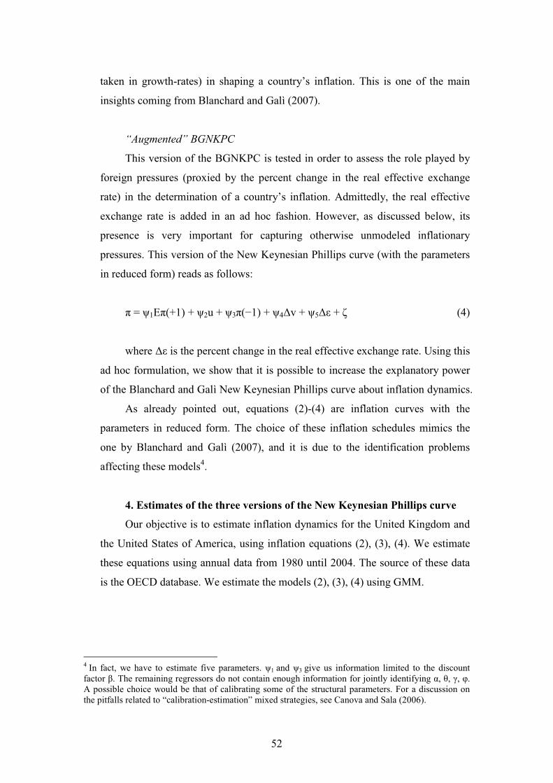
52
taken in growth-rates) in shaping a country’s inflation. This is one of the main
insights coming from Blanchard and Galì (2007).
“Augmented” BGNKPC
This version of the BGNKPC is tested in order to assess the role played by
foreign pressures (proxied by the percent change in the real effective exchange
rate) in the determination of a country’s inflation. Admittedly, the real effective
exchange rate is added in an ad hoc fashion. However, as discussed below, its
presence is very important for capturing otherwise unmodeled inflationary
pressures. This version of the New Keynesian Phillips curve (with the parameters
in reduced form) reads as follows:
= 1E(+1) + 2u + 3(−1) + 4v + 5 + (4)
where is the percent change in the real effective exchange rate. Using this
ad hoc formulation, we show that it is possible to increase the explanatory power
of the Blanchard and Galì New Keynesian Phillips curve about inflation dynamics.
As already pointed out, equations (2)-(4) are inflation curves with the
parameters in reduced form. The choice of these inflation schedules mimics the
one by Blanchard and Galì (2007), and it is due to the identification problems
affecting these models4.
4. Estimates of the three versions of the New Keynesian Phillips curve
Our objective is to estimate inflation dynamics for the United Kingdom and
the United States of America, using inflation equations (2), (3), (4). We estimate
these equations using annual data from 1980 until 2004. The source of these data
is the OECD database. We estimate the models (2), (3), (4) using GMM.
4 In fact, we have to estimate five parameters. 1 and 3 give us information limited to the discount
factor . The remaining regressors do not contain enough information for jointly identifying , , , .
A possible choice would be that of calibrating some of the structural parameters. For a discussion on
the pitfalls related to “calibration-estimation” mixed strategies, see Canova and Sala (2006).
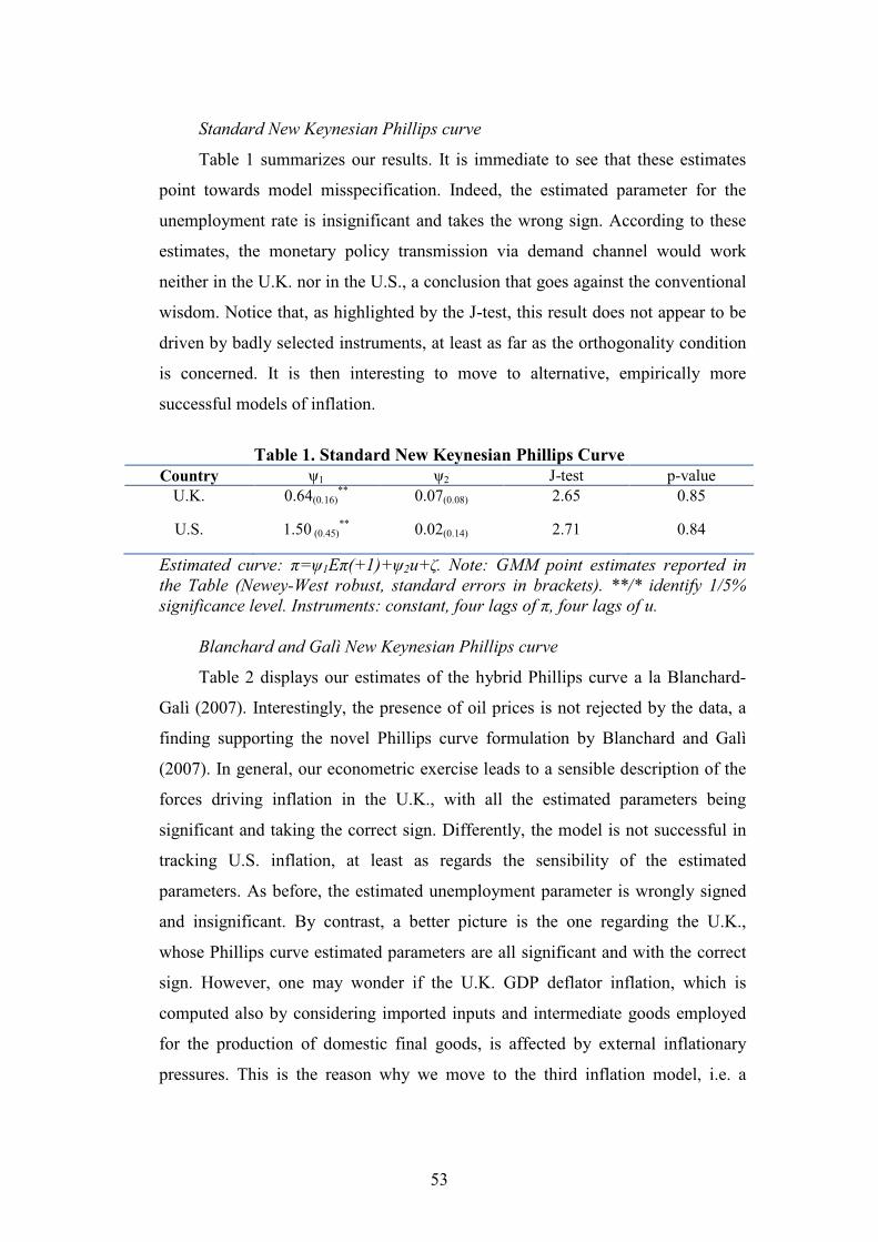
53
Standard New Keynesian Phillips curve
Table 1 summarizes our results. It is immediate to see that these estimates
point towards model misspecification. Indeed, the estimated parameter for the
unemployment rate is insignificant and takes the wrong sign. According to these
estimates, the monetary policy transmission via demand channel would work
neither in the U.K. nor in the U.S., a conclusion that goes against the conventional
wisdom. Notice that, as highlighted by the J-test, this result does not appear to be
driven by badly selected instruments, at least as far as the orthogonality condition
is concerned. It is then interesting to move to alternative, empirically more
successful models of inflation.
Table 1. Standard New Keynesian Phillips Curve
Country 1 2 J-test p-value
U.K. 0.64(0.16)**
0.07(0.08) 2.65 0.85
U.S. 1.50 (0.45)**
0.02(0.14) 2.71 0.84
Estimated curve: =1E(+1)+2u+. Note: GMM point estimates reported in
the Table (Newey-West robust, standard errors in brackets). **/* identify 1/5%
significance level. Instruments: constant, four lags of , four lags of u.
Blanchard and Galì New Keynesian Phillips curve
Table 2 displays our estimates of the hybrid Phillips curve a la Blanchard-
Galì (2007). Interestingly, the presence of oil prices is not rejected by the data, a
finding supporting the novel Phillips curve formulation by Blanchard and Galì
(2007). In general, our econometric exercise leads to a sensible description of the
forces driving inflation in the U.K., with all the estimated parameters being
significant and taking the correct sign. Differently, the model is not successful in
tracking U.S. inflation, at least as regards the sensibility of the estimated
parameters. As before, the estimated unemployment parameter is wrongly signed
and insignificant. By contrast, a better picture is the one regarding the U.K.,
whose Phillips curve estimated parameters are all significant and with the correct
sign. However, one may wonder if the U.K. GDP deflator inflation, which is
computed also by considering imported inputs and intermediate goods employed
for the production of domestic final goods, is affected by external inflationary
pressures. This is the reason why we move to the third inflation model, i.e. a
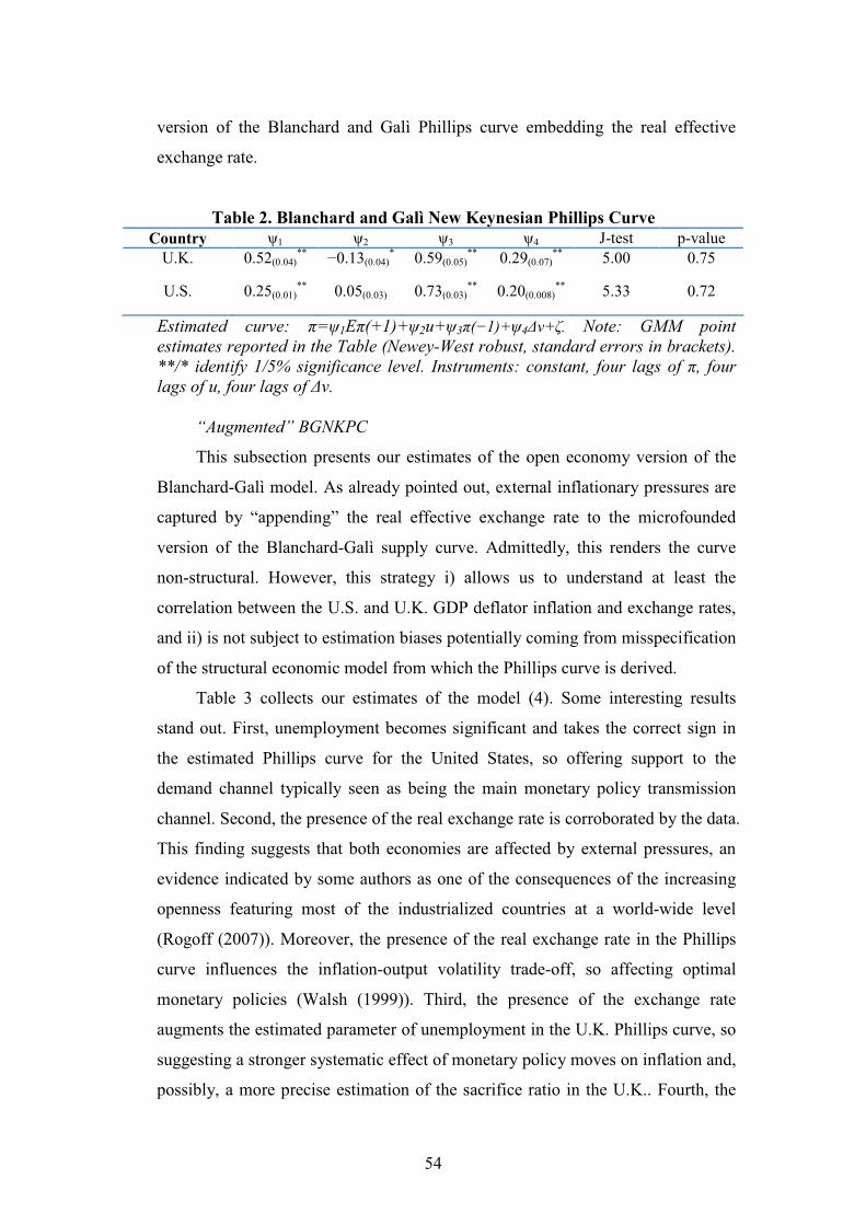
54
version of the Blanchard and Galì Phillips curve embedding the real effective
exchange rate.
Table 2. Blanchard and Galì New Keynesian Phillips Curve
Country 1 2 3 4 J-test p-value
U.K. 0.52(0.04)**
−0.13(0.04)*
0.59(0.05)**
0.29(0.07)**
5.00 0.75
U.S. 0.25(0.01)**
0.05(0.03) 0.73(0.03)**
0.20(0.008)**
5.33 0.72
Estimated curve: =1E(+1)+2u+3(−1)+4v+. Note: GMM point
estimates reported in the Table (Newey-West robust, standard errors in brackets).
**/* identify 1/5% significance level. Instruments: constant, four lags of , four
lags of u, four lags of v.
“Augmented” BGNKPC
This subsection presents our estimates of the open economy version of the
Blanchard-Galì model. As already pointed out, external inflationary pressures are
captured by “appending” the real effective exchange rate to the microfounded
version of the Blanchard-Galì supply curve. Admittedly, this renders the curve
non-structural. However, this strategy i) allows us to understand at least the
correlation between the U.S. and U.K. GDP deflator inflation and exchange rates,
and ii) is not subject to estimation biases potentially coming from misspecification
of the structural economic model from which the Phillips curve is derived.
Table 3 collects our estimates of the model (4). Some interesting results
stand out. First, unemployment becomes significant and takes the correct sign in
the estimated Phillips curve for the United States, so offering support to the
demand channel typically seen as being the main monetary policy transmission
channel. Second, the presence of the real exchange rate is corroborated by the data.
This finding suggests that both economies are affected by external pressures, an
evidence indicated by some authors as one of the consequences of the increasing
openness featuring most of the industrialized countries at a world-wide level
(Rogoff (2007)). Moreover, the presence of the real exchange rate in the Phillips
curve influences the inflation-output volatility trade-off, so affecting optimal
monetary policies (Walsh (1999)). Third, the presence of the exchange rate
augments the estimated parameter of unemployment in the U.K. Phillips curve, so
suggesting a stronger systematic effect of monetary policy moves on inflation and,
possibly, a more precise estimation of the sacrifice ratio in the U.K.. Fourth, the
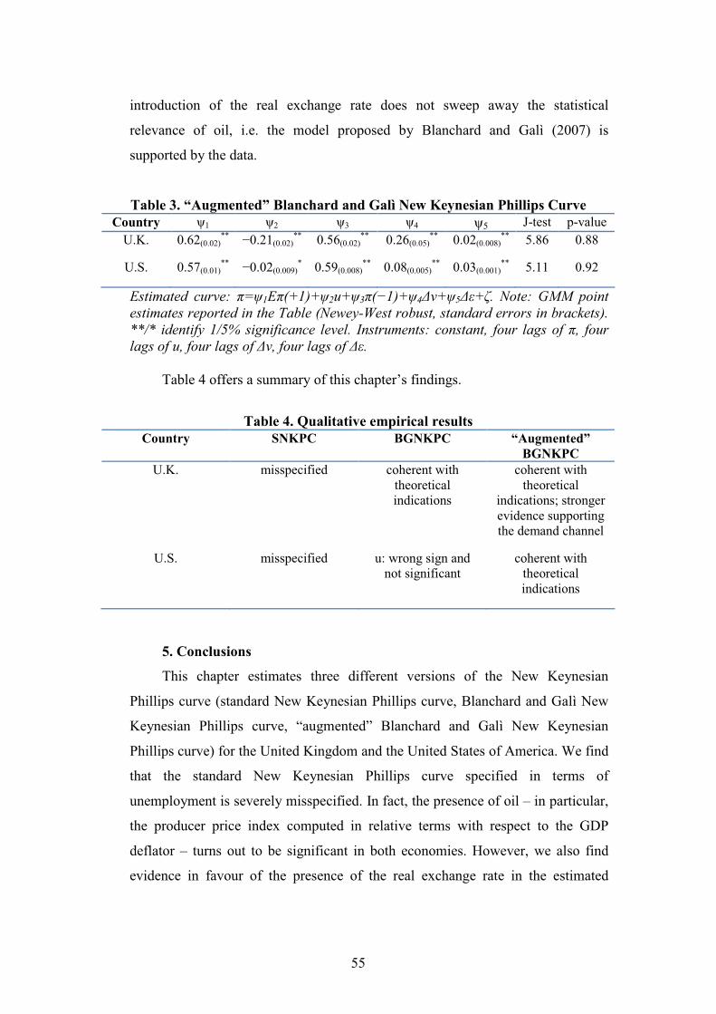
55
introduction of the real exchange rate does not sweep away the statistical
relevance of oil, i.e. the model proposed by Blanchard and Galì (2007) is
supported by the data.
Table 3. “Augmented” Blanchard and Galì New Keynesian Phillips Curve
Country 1 2 3 4 5 J-test p-value
U.K. 0.62(0.02)**
−0.21(0.02)**
0.56(0.02)**
0.26(0.05)**
0.02(0.008)**
5.86 0.88
U.S. 0.57(0.01)**
−0.02(0.009)*
0.59(0.008)**
0.08(0.005)**
0.03(0.001)**
5.11 0.92
Estimated curve: =1E(+1)+2u+3(−1)+4v+5+. Note: GMM point
estimates reported in the Table (Newey-West robust, standard errors in brackets).
**/* identify 1/5% significance level. Instruments: constant, four lags of , four
lags of u, four lags of v, four lags of .
Table 4 offers a summary of this chapter’s findings.
Table 4. Qualitative empirical results
Country SNKPC BGNKPC “Augmented”
BGNKPC
U.K. misspecified coherent with
theoretical
indications
coherent with
theoretical
indications; stronger
evidence supporting
the demand channel
U.S. misspecified u: wrong sign and
not significant
coherent with
theoretical
indications
5. Conclusions
This chapter estimates three different versions of the New Keynesian
Phillips curve (standard New Keynesian Phillips curve, Blanchard and Galì New
Keynesian Phillips curve, “augmented” Blanchard and Galì New Keynesian
Phillips curve) for the United Kingdom and the United States of America. We find
that the standard New Keynesian Phillips curve specified in terms of
unemployment is severely misspecified. In fact, the presence of oil – in particular,
the producer price index computed in relative terms with respect to the GDP
deflator – turns out to be significant in both economies. However, we also find
evidence in favour of the presence of the real exchange rate in the estimated
56
supply curves. Importantly, such a regressor helps identifying the value of other
estimated parameters in the two schedules under investigation.
It seems to us that the Blanchard and Galì New Keynesian Phillips curve,
above all when interpreted in an open economy fashion, may very well be a
credible alternative to the standard, output gap-driven supply curve. This calls for
further analysis concerning optimal monetary policy in the presence of explicitly
modelled supply shocks on the one hand, and the role played by such supply
shocks in triggering inflation and business cycle fluctuations on the other hand.
These efforts belong to our research agenda.
57
References
Blanchard O., Galì J. (2007), “Real Wage Rigidities and the New
Keynesian Model,” Journal of Money, Credit and Banking, Supplement to vol.
39(1), pp. 35-65.
Canova, F., and Sala L. (2006), “Back to Square One: Identification Issues
in DSGE Models,” Working Paper Series 583, European Central Bank.
Clarida R., Galì J., Gertler M. (1999), “The Science of Monetary Policy:
A New Keynesian Perspective,” Journal of Economic Literature, vol. 37(4), pp.
1661-1707.
Clarida R., Galì J., Gertler M. (2001), “Optimal Monetary Policy in Open
vs. Closed Economies: An Integrated Approach,” American Economic Review, vol.
91(2), pp. 248-252.
Erceg C., Henderson D., Levin A. (2000), “Optimal Monetary Policy with
Staggered Wage and Price Contracts,” Journal of Monetary Economics, 46(2), pp.
281-313.
Gordon R. (1997), “The Time Varying NAIRU and Its Implications for
Economic Policy,” Journal of Economic Perspectives, vol. 11(1), pp. 11-32.
Hall R. (2005), “Employment Fluctuations with Equilibrium Wage
Stickiness,” American Economic Review, vol. 95(1), pp. 50-64.
Mankiw N.G. (2001), “The Inexorable and Mysterious Tradeoff between
Inflation and Unemployment,” Economic Journal, 111, C45-C61.
Roberts J. (1995), “New Keynesian Economics and the Phillips Curve,”
Journal of Money, Credit and Banking, vol. 27(4), pp. 975-984.
Roberts J. (2006), “Monetary Policy and Inflation Dynamics,” International
Journal of Central Banking, vol. 2(3), pp. 193-230.
Rogoff, K. (2007), “Impact of Globalization on Monetary Policy,” in The
New Economic Geography: Effects and Policy Implications, Federal Reserve
Bank of Kansas City.
Smets F., Wouters R. (2003), “An Estimated Dynamic Stochastic General
Equilibrium Model of the Euro Area,” Journal of the European Economic
Association, vol. 1(5), pp. 1123-1175.
Steinsson J. (2003), “Optimal Monetary Policy in an Economy with
Inflation Persistence,” Journal of Monetary Economics, vol. 50(7), pp. 1425-1456.
58
Walsh C. (1999), “Monetary Policy Trade-Offs in the Open-Economy,”
University of California at Santa Cruz, manuscript.
Woodford M. (2003), Interest and Prices: Foundations of a Theory of
Monetary Policy, Princeton University Press.
59
Data appendix
The data used come from: a)OECD Economic Outlook for GDP deflator;
b)OECD Main Economic Indicator for PPI and real effective exchange rate;
c)OECD Labour Force Survey for standardised unemployment rate.
We define the variables of the equations (2)-(4) in the following way:
Inflation [(-1) and E(+1)]: for inflation we use the annual percent
change in the GDP price deflator.
= [GDP −GDP(−1)] / GDP(−1)·100
where GDP is gross domestic product price deflator.
For inflation at the time minus one, (−1), we consider the realized inflation
at the previous year.
For future expected inflation, E(+1), we consider the realized inflation at
the next year.
Unemployment (u): we consider unemployment using the percent
standardised unemployment rate.
Percent change in the price of nonproduced input (v): we define the
percent change in the price of nonproduced input as the annual percent change in
the PPI relative to the GDP price deflator.
v = [(PPI/GDP) − (PPI(−1)/GDP(−1))] / (PPI(−1)/GDP(−1))·100
v: annual percent change in the price of nonproduced input.
PPI: producer price index.
GDP: gross domestic product price deflator.
Percent change in the real effective exchange rate (): we define the
percent change in the real effective exchange rate as the annual percent change in
the real effective exchange rate.
= [ − (−1)] / (−1)·100
: annual percent change in the real effective exchange rate.

60

61
CHAPTER 3
“Assessing the Role of Oil Price Shocks
in a New Keynesian Model”
1. Introduction
The New Keynesian model (for a textbook presentation see Woodford
(2003)) is the core analytical tool to study monetary policy and the business cycle
nowadays. A key schedule of this model is the New Keynesian Phillips curve
(NKPC henceforth). In the standard form the NKPC reads t=Ett+1+k(yt−yt*),
where is inflation, identifies firms’ discount factor, Et expresses expectations
taken at time t (i.e. with an information set updated up to t), y represents current
GDP taken in logs, y* is the log of the natural level of output (i.e. the second best
output), and (y−y*) is the output gap.
Many economists have highlighted an important lack afflicting the NKPC
(e.g. Mankiw (2001)). This lack is the absence of a trade-off between the
stabilization of inflation and the stabilization of the welfare-relevant output gap
(i.e. the gap between current and the first best level of output), when a supply
shock strikes the economy. The reason is the following. In the standard New
Keynesian model the difference between the first and the second best output
remains always constant. Therefore, if a central bank stabilizes simultaneously
inflation and the output gap, in the same time it stabilizes the welfare-relevant
output gap.1 Blanchard and Galì (2007) call this feature of the standard New
Keynesian model “divine coincidence”. Interestingly, they show that, if non trivial
real imperfections are endogenized in the New Keynesian model, the “divine
coincidence” does not work anymore. In particular they include real wage
rigidities in the model determining a break of the constant relation between the
first and the second best output. The effect is that the policy maker can not
stabilize simultaneously inflation and the welfare-relevant output gap. Because of
real wage rigidities, a trade-off between inflation and the welfare-relevant output
gap arises in front of central banker in the presence of a supply shock. From their
assumptions, Blanchard and Galì (2007) obtain a new version of the New
1 The second best output level is the one that would prevail under flexible prices in the presence of real
distortions such as monopolistic competition. By contrast, the first best output level is the one that
would realize under fully flexible prices and perfect competition in all markets.
62
Keynesian Phillips curve (BGNKPC henceforth), characterized by the presence of
the real price of a nonproduced input (e.g. oil) among the independent variables.
Interestingly, this feature allows a researcher to investigate the role played by oil
shocks in shaping inflation and the business cycle, a role object of an intense
debate in the literature [(Blanchard and Galì (2007); Nakov and Pescatori (2007)].
This chapter estimates and simulates a small-scale DSGE New Keynesian
model including the BGNKPC for the United States in the quarterly data sample
1984:1−2007:4. We then perform factual and counterfactual simulations to gauge
the role played by different shocks on inflation, unemployment and policy rate.
Our main findings are the followings. First, oil price shocks have played an
important role in explaining inflation fluctuations in the U.S. economy in the last
two decades. In particular, the explained variance of the U.S. inflation due to such
shocks amounts to 9.27 percent. This is due both to the direct impact that oil price
shocks exert on GDP inflation and the indirect impact working throughout their
influence on the U.S. systematic monetary policy, but it is largely due to the
former. By contrast, the contribution of oil price shocks in determining
unemployment fluctuations has been very modest, i.e. 0.05 percent. Moreover the
driving shocks for inflation and unemployment are respectively non-oil supply
shock (81.08%) and demand non-policy shock (98.52%). Second, stronger
reactions to oil price swings than the ones historically observed would not have
improved the stabilization of inflation and unemployment. Third, the best result in
terms of stabilization of inflation and unemployment is conditional to the type of
shock hitting the economy. In particular the best result is obtained by a
“progressive central bank” (i.e. a central bank which reacts strongly to
unemployment and weakly to inflation) in the presence of oil price shock, and by
an “interventionist central bank” (i.e. a central bank which reacts strongly both to
inflation and to unemployment) in the presence of monetary policy shock. Fourth,
the more forward-looking the firms are, the more stable the economy is in the
presence of oil price shock.
This chapter develops as follows. Section 2 underlines the economic
literature about oil related to our work. Section 3 presents the version of small-
scale DSGE New Keynesian model including the BGNKPC. Section 4 proposes
the estimates of this model. In the section 5 we perform different counterfactual
63
simulations to gauge the role of different monetary policy rules and different
inflation expectations hypotheses in explaining inflation, unemployment and short
term interest rate fluctuations. Section 6 presents variance decomposition data to
identify key-shocks. Section 7 compares our model with that of Nakov and
Pescatori (2007). Section 8 concludes.
2. Literature about oil related to our work
Our work is an empirical work which aims to focus the role of oil price
shock in explaining inflation and unemployment fluctuations. To conduct this
analysis and to assess the found results we identify some links with other
economic papers which tackle the oil subject in macroeconomic key. On the
empirical hand useful references for us are Darby (1982), Hamilton (1983),
Burbidge and Harrison (1984). These authors find that increases of oil price are
followed by decreases of U.S. output growth (Hamilton (1983)), by decreases of
growth rate of the real GNP for the U.S. and other countries (Darby (1982)), by
rises of inflation and decreases of industrial production for the U.S. and other
countries (Burbidge and Harrison (1984)). This authors signal an important role of
oil price shocks in explaining inflation and output fluctuations. The conclusions of
Hamilton (1983) are called into question by Bernanke, Gertler and Watson (1997).
According to these authors the main cause of U.S. recessions after World War II
was a restrictive monetary policy more than oil price rises. In support to the
Bernanke, Gertler and Watson’s thesis there are two papers: Barsky and Kilian
(2001) and Kilian (2005). These authors claim that the stagflation phenomenon of
the seventies was generated essentially by monetary dynamics, while the role of
oil price increases was limited. Our analysis allows us to affirm that in the period
from 1984 to 2007 the oil price shocks have played a role which appears irrelevant
in determining unemployment fluctuations, but is important in determining
inflation fluctuations. On the theoretical hand relevant papers which incorporate
oil in a macroeconomic framework are written by Rotemberg and Woodford
(1996), Finn (1995, 2000), Leduc and Sill (2004), Carlstrom and Fuerst (2005).
All these papers have in common that they suppose an exogenous path for oil
price. This approach appears unsatisfactory, because in a model conceived in this
way for policy maker there is not a trade-off between stabilizing inflation and
64
stabilizing the welfare-relevant output gap in the presence of oil price shock. A
solution for this lack is proposed by Nakov and Pescatori (2007), who make
endogenous the optimal oil price markup of the dominant supplier of oil (e.g.
OPEC). This solution allows two authors to create a trade-off between stabilizing
inflation and stabilizing the welfare-relevant output gap in the presence of oil
price shock. As we argue in the introduction, Blanchard an Galì (2007) reach the
same result introducing in their model real wage rigidities. The model which we
analyse tries to take in both i) Nakov and Pescatori’s proposal (in fact in our
framework we model the percent change in the real price of oil as a function of
past change in unemployment rate, past short term interest rate and past percent
change in the real price of oil) and ii) Blanchard and Galì solution using the
BGNKPC, which incorporates the real price of oil.
3. A small-scale DSGE New Keynesian model
The small-scale DSGE New Keynesian model we consider is composed by
four equations.
The first equation is the BGNKPC2. This equation reads as follows:
= 1E(+1) + 2u + 3(−1) + 4v + (1)
where represents current inflation, E(+1) is expected future inflation, u
is the change in unemployment rate, (−1) is past inflation, v is the percent
change in the real price of oil and is the inflation shock3.
The second equation is the Euler equation with unemployment rate in place
of output gap4:
u = 5u(−1) + 6[i−E(+1)] + (2)
2 With respect to the original version of the BGNKPC, we replace unemployment in levels with its first
difference to capture the transmission mechanism going from unemployment to inflation in a more
satisfactory fashion from an empirical standpoint. 3 In the following part of the chapter we refer to the change in unemployment rate and the percent
change in the real price of oil respectively as unemployment and real price of oil. 4In order to augment the degree of comparability among different equations of the DSGE New
Keynesian model, we substitute the output gap with the change in unemployment rate. As postulated by
the Okun’s law, these two macroeconomic variables are very correlated. Gordon (1997) and Roberts
(1995, 2006) propose a similar solution with respect to the New Keynesian Phillips curve.
65
where i is short term interest rate and is the unemployment shock.
The third equation is the Taylor rule [Taylor (1993)]:
i = 7 + 8u + 9i(−1) + (3)
where is the monetary policy shock.
The fourth equation refers to the real price of oil:
v = 10v(– 1) + 11u(–1) + 12i(–1) + (4)
where is the oil price shock.
All coefficients are expected to take a positive value except for 2, 8, 11,
12 which are assumed to be negative.
4. Estimates
We estimate the small-scale DSGE New Keynesian model expressed by the
equations (1)−(4) for the U.S. economy using quarterly data which span the
sample 1984:1−2007:4. The choice of 1984:1 as the first quarter of our analysis is
justified by our willingness to study the U.S. economy in a stable policy regime
[Clarida, Galì, Gertler (2000)]. We assume that the four kinds of shock are
uncorrelated. Following this assumption we estimate the equations (1)−(4)
separately. In particular we estimate the BGNKPC, the Euler equation and the
Taylor rule by GMM; while we estimate the equation (4) by OLS.
The table 1 displays the estimates for the U.S.. The estimated coefficients
exhibit signs in line with to the economic wisdom and are significant at 5% (but
6 and 11 are significant at 10%). The only exception is represented by the
coefficient on unemployment in the BGNKPC which takes a positive, but not
significant, sign.
According to our estimates in the BGNKPC expected future inflation is
predominant in explaining inflation dynamics with respect to past inflation. The
real price of oil exerts a positive effect on inflation, with an estimated coefficient
equal to 0.05.
66
The estimate of equation (2) (i.e. the Euler equation) shows that
unemployment is highly persistent. The expected future interest rate influences
positively current unemployment.
The estimate of equation (3) (i.e. the Taylor rule) gives results coherent with
our expectations. The coefficient on inflation is positive, signalling a positive
impact on the short term interest rate by the side of inflation. Importantly, the
Taylor principle is satisfied. This principle requires that in the long-run the short
term interest rate reacts more than one to one to a change in inflation. The long-
run coefficient on inflation in the Taylor rule is equal to [7/(1−9)], and it has to
be higher than one to guarantee that the move of the policy rate in a certain
direction is followed by the move of the real interest rate in the same direction.
According to our estimates, [7/(1−9)]=3.28. Still focusing on the Taylor rule,
unemployment exerts a very strong negative impact on the short term interest rate
in the U.S., highlighting a very active role played by the FED in contrasting
negative shocks on the business cycle. Moreover the short term interest rate is
characterized by a high level of persistence.
Finally, the estimate of equation (4) suggests an important level of
persistence in the path of the real price of oil. Besides the effects played by past
short term interest rate and past unemployment on the real price of oil are both
negative. This is due to the fact that, when past short term interest rate or past
unemployment increases, the oil demand falls determining a reduction of the real
price of oil. In particular the negative impact of past unemployment is more
intensive with respect to that of past short term interest rate.
5. Impulse response functions
5.1. Standard case:
We estimate impulse response functions of the small-scale DSGE New
Keynesian model (1)−(4) using the estimated coefficients presented in the
previous section (we label this scenario as “standard case”)5. We assume that four
kinds of shock can hit the economy: a) inflation shock, which hits the BGNKPC;
5 Here and in the subsequent simulations we calibrate 2=−0.20, following Roberts (2006). Moreover,
although the estimated value of coefficient 8 is −2.17, we calibrate this coefficient equal to −1.245, i.e.
the average between −1.49 (i.e. 8 + 28, where 8 is the estimated standard deviation for 8) and −1
(i.e. the value attributed to 8 by Orphanides and Williams (2006)).
67
b) unemployment shock, which works via Euler equation; c) monetary policy
shock, which acts on Taylor rule equation (3); d) oil price shock, which influences
equation (4). We assume that estimated residuals may be interpreted as structural
shocks. Here and in the remaining part of the chapter we assume that, in
estimating the impulse response functions, each innovation is equal to a standard
error as estimated in this chapter. The period of simulation is fixed in forty
quarters.
We are interested in understanding the paths of inflation, unemployment and
short term interest rate in the presence of each of these shocks. The figures 1−4
display the estimated impulse response functions.
Oil price shock:
The response of U.S. inflation, when an oil price shock hits the U.S.
economy, is positive.
This variable jumps to about 0.31 percent above its steady state value and
then it begins to decline. After one year and one quarter after this shock it is equal
to −0.02 percent with respect to the steady state value. U.S. inflation returns to its
steady state value after six years and one quarter after this shock.
Differently U.S. unemployment responds negatively in reaction to this kind
of shock. Initially unemployment goes to about −0.0003 percent below its steady
state value. Then it increases and after one year and one quarter is above the
steady state value of about 0.0016 percent. Subsequently it declines and returns to
its steady state value after seven years after this shock.
Initially U.S. short term interest rate responds in positive way to oil price
shock. It jumps to 0.072 percent above its steady state value. It continues to
increase until 0.09 percent after three quarters after the shock and then it declines
and comes back to its steady state value after eight years and three quarters after
this shock.
The oil price shock determines an initial increase of the real price of oil to
about 4.5 percent with respect to its steady state value. Afterwards this variable
decreases to −0.1 percent with respect to its steady state value after one year and
one quarter after the shock. Then it goes newly to its steady state value after three
years after this shock.
68
Among the variables analysed we see that, in reaction to oil price shock, the
real price of oil is characterized by more variance, while U.S. short term interest
rate is settled by more persistence.
Inflation shock:
The initial effect of inflation shock on inflation is higher than that on short
term interest rate or unemployment or real price of oil. After this shock U.S.
inflation jumps above its steady state value. Then it decreases quickly in the way
that after four quarters is about −0.05 percent with respect to steady state. Inflation
returns to steady state after about six years after this shock.
The inflation shock exerts a very low effect on U.S. unemployment. In fact
the maximum deviation of this variable from steady state is equal to about 0.0041
percent after one year after this shock. Unemployment returns to its steady state
value after about nine years after this shock.
U.S. short term interest rate augments to about 0.225 percent with respect to
its steady state value in consequence of inflation shock; afterwards it decreases
and reassumes its steady state value after eight years and half after this shock.
After three quarters after the inflation shock, the real price of oil decreases to
−0.14 percent with respect to steady state. Then it increases and reassumes its
steady state value after eight years and one quarter after this shock.
Among the variables analysed we see that, in reaction to inflation shock,
U.S. inflation is characterized by more variance, while U.S. unemployment is
settled by more persistence.
Unemployment shock:
Inflation goes to about −0.058 percent below its steady state value after the
unemployment shock. Then, after one year and half, it increases to about 0.076
percent with respect to its steady state value and then it returns to steady state
value after eight years and half after this shock.
While the initial response of U.S. inflation to unemployment shock is
negative, U.S. unemployment follows a positive path. U.S. unemployment reaches
a value of about 0.14 percent above its steady state value and then declines to
69
about −0.002 percent below the steady state after two years. U.S. unemployment
comes back to its steady state value after five years and half after this shock.
Initially U.S. short term interest rate reacts in negative manner to
unemployment shock. In fact it goes to about −0.19 percent with respect to its
steady state value. Then it still declines to about −0.29 percent after three quarters.
From that point it increases and reassumes the steady state value after eight years
and three quarters after this shock.
The real price of oil goes to −0.55 percent below its steady state value after
two quarters after this shock. Then it increases to 0.12 percent above steady state
after about one year and three quarters. Afterwards it decreases and comes back to
its steady state value after nine years after this shock.
Among the variables considered we see that, in reaction to unemployment
shock, the real price of oil is characterized by more variance and more persistence.
Monetary policy shock:
The initial response of U.S. inflation to monetary policy shock is negative.
U.S. inflation goes to about −0.115 percent with respect to its steady state value.
Then it declines further on to about −0.132 percent after two quarters and
subsequently increases until returning newly to its steady state value after eight
years and three quarters after this shock.
Initially U.S. unemployment responds in positive way to monetary policy
shock. It jumps to about 0.0049 percent above its steady state value. Then it still
increases to about 0.0072 percent above the steady state after one year after this
shock. From that point U.S. unemployment declines and returns to steady state
value after nine years after this shock.
After the monetary policy shock the initial response of U.S. short term
interest rate is positive. In fact this variable augments to about 0.42 percent above
its steady state value. Subsequently it decreases continually and returns to steady
state after eight years and one quarter after this shock.
In response to monetary policy shock the real price of oil decreases to
−0.235 percent below its steady state value after three quarters. Then it increases
until returning to steady state after eight years and half.
70
Among the variables examined we see that, in reaction to monetary policy
shock, U.S. short term interest rate is characterized by more variance, while U.S.
unemployment is settled by more persistence.
The table 2 synthesizes all these results.
5.2. Alternative Taylor rules
We simulate the equations (1)−(4) performing different monetary policy
rules or assuming different weights for backward−looking and forward−looking
expectations in the BGNKPC. We consider five hypothetical scenarios: 1)
different responses of short term interest rate to inflation in the Taylor rule (case
called “Taylor rule I”); 2) different responses of short term interest rate to
unemployment in the Taylor rule (case called “Taylor rule II”); 3) different
responses of short term interest rate to inflation and unemployment in the Taylor
rule (case called “mixed Taylor rules I and II”); 4) different responses of short
term interest rate to real price of oil in the Taylor rule (case named “Taylor rule
III”); 5) different coefficients on past inflation and expected future inflation in the
BGNKPC (case called “Different inflation expectations”).
Taylor rule I:
This counterfactual analysis deviates from the standard case analysed in the
section 5.1 for the reason that we suppose that the monetary authority reacts to
inflation differently with respect to the value estimated for 7. We assume two
hypothetical situations. The first situation consists in an aggressive response of the
central bank to inflation. In this case we assume 7=0.35
6. The second situation
hypothesizes that the monetary authority reacts weaker than reality to inflation. In
this case 7=0.11
7. We compare these two hypothetical scenarios and that
represented by the standard case (which is the benchmark). In particular, we try to
understand the different effects of oil price shock and monetary policy shock on
inflation, unemployment and short term interest rate under the two hypothetical
cases and the standard case. The results are represented in the figure 5.
67
´=7+27, where 7 is the estimated standard deviation for 7 in the Taylor rule.
77
´´=7−27.
71
For the U.S. economy a more aggressive behaviour of the central bank
against inflation does not give a general advantage in terms of inflation variance’s
reduction. In fact, if an oil price shock hits the U.S. economy, inflation exhibits
lower variance in the case of weak response of central bank to inflation (while in
the presence of this shock all the three scenarios analysed produce the same result
in terms of inflation persistence’s reduction). Following this shock, also the
standard case realizes a better performance in terms of inflation variance’s
reduction with respect to the case involving strong reaction to inflation. Instead, in
the presence of monetary policy shock, the appropriate behaviour to stabilize U.S.
inflation quickly and with lower variance is the strong response of short term
interest rate to inflation.
As for U.S. inflation, also for U.S. unemployment there is not only one best
central bank’s response to inflation to reduce variance, whatever is the shock
involved. In fact, if an oil price shock hits the U.S. economy, the best strategy for
the central bank to minimize the variance of unemployment is to react in weak
way to inflation. On the contrary, if a monetary policy shock realizes, the best
strategy for unemployment variance’s reduction is to react in strong way to
inflation. In terms of unemployment persistence’s reduction, the best strategy is to
respond strongly to inflation in the presence of whatever shock.
The best strategy for the central bank to reduce the variance of U.S. short
term interest rate is: i) the weak response to inflation in the presence of oil price
shock; ii) the strong response to inflation in the presence of monetary policy
shock. The best strategy for the monetary authority to minimize the persistence of
U.S. short term interest rate is the strong response to inflation in the presence of
whatever shock.
The results which we have found are displayed in the table 3.
Taylor rule II:
This counterfactual analysis differs from the standard case examined in the
section 5.1. because now we suppose that the monetary authority can react to
unemployment differently with respect to the value estimated for 8. We assume
two hypothetical cases. The first case consists in a strong reaction of the central
72
bank to unemployment. In this case we assume 8=−1.49
8. The second case
hypothesizes that the monetary authority reacts more weakly to unemployment. In
this case 8=−1
9. We compare these two hypothetical cases and the standard case
in terms of inflation, unemployment and short term interest rate’s adjustment
paths in the presence of oil price shock and monetary policy shock.
The results are represented in the figure 6.
If an oil price shock comes about, the strong response to unemployment is
the best strategy to reduce the variance of unemployment and short term interest
rate. Instead, in the presence of oil price shock, the three strategies under
investigation produce the same result in terms of inflation variance’s reduction.
In the presence of monetary policy shock the best strategy for the central
bank to reduce variance of inflation, unemployment and short term interest rate is
the strong response to unemployment.
Moreover, in the presence of whatever shock, the strong response to
unemployment, the weak response to unemployment and the standard case realize
the same results in terms of persistence’s reduction for inflation, unemployment
and short term interest rate.
The table 4 summarizes the results which we have found.
Mixed Taylor rules I and II:
In this scenario we assume that the central bank reacts to inflation and
unemployment using mixed strategies arisen from the jointly consideration of the
Taylor rule I and Taylor rule II cases. In particular we identify four situations
characterized by different values assigned to parameters 7 and8:
1) 7=0.35 and 8=−1. In this case the central bank fights aggressively
inflation and contrasts weakly unemployment (case called “conservative central
bank”, CCB henceforth);
2) 7=0.11 and 8=−1.49. In this case the central bank fights weakly
inflation and contrasts strongly unemployment (case called “progressive central
bank”, PCB henceforth);
88
´=8+28, where 8 is the estimated standard deviation for 8 in the Taylor rule.
9 Orphanides and Williams (2006) impose this value in calibrating an equation very similar to our.
73
3) 7=0.11 and 8=−1. In this situation the central bank fights weakly both
inflation and unemployment (case called “laissez-faire central bank”, LFCB
henceforth);
4) 7=0.35 and 8=−1.49. In this situation the central bank contrasts
strongly both inflation and unemployment (case called “interventionist central
bank”, ICB henceforth).
The results are depicted in the figures 7−8.
In the presence of oil price shock, PCB is the best response of the central
bank to stabilize inflation, unemployment and short term interest rate.
In the presence of monetary policy shock, ICB represents the best reaction of
the central bank to stabilize inflation, unemployment and short term interest rate.
The best responses identified in this section are more efficacious in terms of
stabilization with respect to the responses generated by the standard case.
The table 5 summarizes the results which we have found.
Taylor rule III:
We analyse the adjustment paths towards the steady state values of U.S.
inflation, unemployment and short term interest rate assuming a different structure
of the Taylor rule. Opposite to the equation (3), we include the real price of oil
among the independent variables of the Taylor rule. Now we assume that the
central bank considers also this variable in moving short term interest rate. For
this reason the new Taylor rule takes this form:
i = 7 + 8u + 9i(−1) + oilv + (5)
The standard case is characterized by oil equal to zero. Now we calibrate oil
to represent two alternative hypothetical strategies in response to real price of oil.
We call the situations with oil´=0.10 and oil
´´=0.20 respectively “weak response
to real price of oil” and “strong response to real price of oil”10
. We compare U.S.
inflation, unemployment and short term interest rate’s adjustment paths in the
10oil
´ and oil
´´ are calibrated following Bernanke, Gertler and Watson (2004) and Carlstrom and Fuerst
(2005).
74
presence of oil price shock and monetary policy shock under the standard, weak
response to real price of oil, strong response to real price of oil cases.
The results are represented in the figure 9.
If an oil price shock hits the economy, the more variance’s reduction for
inflation is obtained by interest rate’s no response in reaction to real price of oil
(i.e. the standard case). Moreover, when an oil price shock strikes the economy,
also U.S. unemployment and short term interest rate require no response of short
term interest rate to real price of oil to minimize their variance. Furthermore, in
the presence of oil price shock, the strong response of short term interest rate in
reaction to real price of oil produces always the worst result in terms of inflation,
unemployment, short term interest rate variance’s reduction. Instead, in the
presence of oil price shock, the strong response to real price of oil, the weak
response to real price of oil and the standard case realize the same results in terms
of inflation, unemployment and short term interest rate persistence’s reduction.
In the presence of monetary policy shock, the strong response to real price of
oil realizes the more variance and persistence’s reduction for inflation,
unemployment and short term interest rate.
These results are displayed in the table 6.
5.3. Different inflation expectations:
We simulate the equations (1)−(4) assuming different values for coefficients
on expected future inflation and past inflation, 1 and 3, in the BGNKPC. The
calibration of these two parameters allows us to reproduce three cases: i) standard
case, in which 1 and 3 take the estimated values; ii) more forward-looking case
(with respect to the standard case, MFL henceforth), in which 1=0.925 and
3=0.075; iii) purely forward-looking case (PFL henceforth), in which 1=1 and
3=0.
This exercise tries to clarify the role played by inflation expectations on
inflation, unemployment and short term interest rate paths in the presence of oil
price shock.
The results are displayed in the figure 10.
Under the PFL case U.S. inflation returns to its steady state value with lower
variance with respect to the MFL and standard cases, in the presence of oil price
75
shock. Inflation expectations performed in purely forward-looking manner reduce
the cost of disinflation. This fact is coherent with the idea that the more credible
the commitment offered by the monetary authority to economic agents is, the
more forward-looking firms’ inflation expectations are. When the credibility of
commitment is very high, firms’ inflation expectations are only forward-looking.
Instead, in the presence of oil price shock, the PFL, MFL and standard cases
assure substantially the same performance in terms of inflation persistence’s
reduction.
Analogous tendencies concern U.S. unemployment and short term interest
rate. When an oil price shock hits the U.S. economy, the PFL case ensures
unemployment and short term interest rate paths with the minimum variance. In
regard to unemployment and short term interest rate, the PFL, MFL and standard
cases offer identical results in terms of persistence’s reduction.
The table 7 synthesizes the results which we have described.
6. Variance decomposition
We compute the variance decomposition of U.S. inflation, unemployment
and short term interest rate to deliver the key-shocks which generate fluctuations
of these variables. We show that in the standard case the role played by oil price
shock in determining fluctuations is important for U.S. inflation. Instead it appears
to be irrelevant for U.S. unemployment and short term interest rate. U.S. inflation
fluctuations are explained by oil price shock for 9.27 percent. Besides oil price
shock is responsible of only 0.05 percent of U.S. unemployment fluctuations and
of 2.87 percent of short term interest rate fluctuations. Our results are different in
terms of oil price shock’s impact in explaining inflation and short term interest
rate variance with respect to those found by Nakov and Pescatori (2007). In
particular, according to Nakov and Pescatori (2007), oil price shocks are
altogether responsible of 33.54 percent of inflation variance and 13.96 percent of
short term interest rate variance.
On the other hand, monetary policy shock explains an important fraction of
U.S. inflation variance and a little fraction of U.S. unemployment variance. In fact
monetary policy shock influences U.S. inflation and unemployment fluctuations
respectively by 6.48 and 1.07 percent. Notably, also Christiano, Eichenbaum and
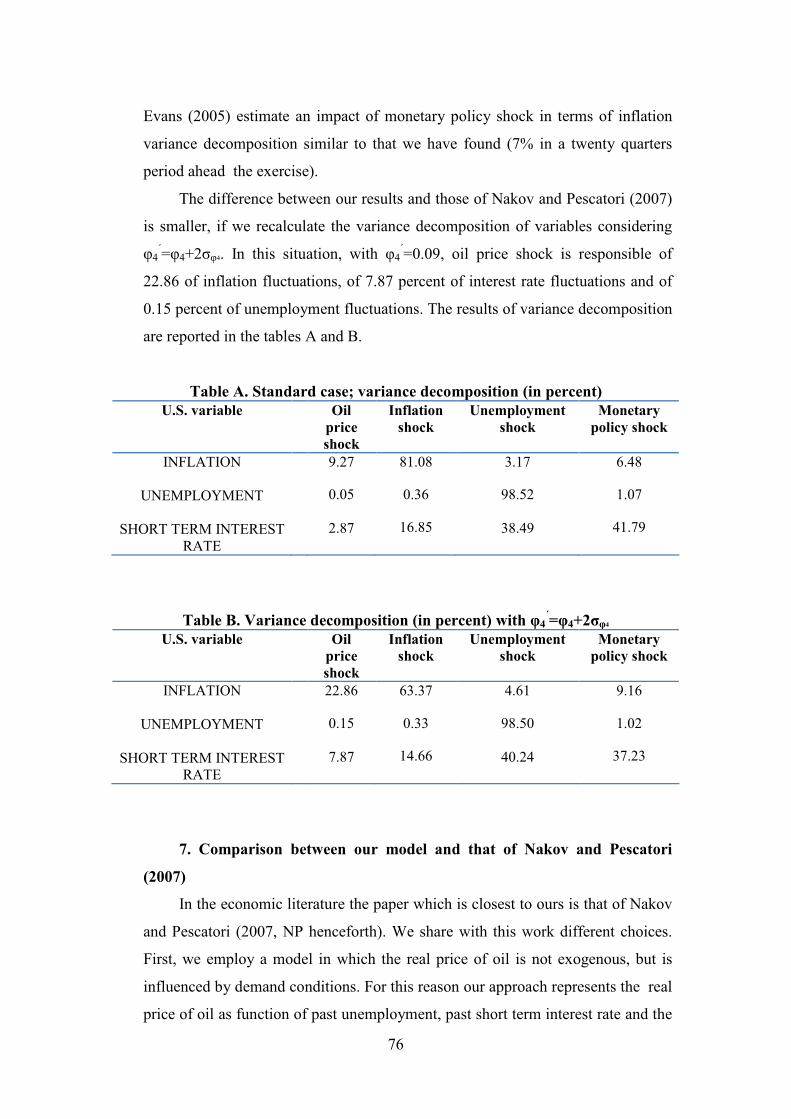
76
Evans (2005) estimate an impact of monetary policy shock in terms of inflation
variance decomposition similar to that we have found (7% in a twenty quarters
period ahead the exercise).
The difference between our results and those of Nakov and Pescatori (2007)
is smaller, if we recalculate the variance decomposition of variables considering
4´=4+24. In this situation, with 4
´=0.09, oil price shock is responsible of
22.86 of inflation fluctuations, of 7.87 percent of interest rate fluctuations and of
0.15 percent of unemployment fluctuations. The results of variance decomposition
are reported in the tables A and B.
Table A. Standard case; variance decomposition (in percent)
U.S. variable Oil
price
shock
Inflation
shock
Unemployment
shock
Monetary
policy shock
INFLATION
UNEMPLOYMENT
SHORT TERM INTEREST
RATE
9.27
0.05
2.87
81.08
0.36
16.85
3.17
98.52
38.49
6.48
1.07
41.79
Table B. Variance decomposition (in percent) with 4´=4+24
U.S. variable Oil
price
shock
Inflation
shock
Unemployment
shock
Monetary
policy shock
INFLATION
UNEMPLOYMENT
SHORT TERM INTEREST
RATE
22.86
0.15
7.87
63.37
0.33
14.66
4.61
98.50
40.24
9.16
1.02
37.23
7. Comparison between our model and that of Nakov and Pescatori
(2007)
In the economic literature the paper which is closest to ours is that of Nakov
and Pescatori (2007, NP henceforth). We share with this work different choices.
First, we employ a model in which the real price of oil is not exogenous, but is
influenced by demand conditions. For this reason our approach represents the real
price of oil as function of past unemployment, past short term interest rate and the
77
past real price of oil. In this way we make endogenous the real price of oil as in
NP (2007). Second, we estimate the coefficients of our model. The estimators
employed are GMM for the BGNKPC, the Euler equation and the Taylor rule and
OLS for the equation of the real price of oil. NP (2007) estimate their model with
Bayesian techniques. This fact give us the possibility of assessing the impact of oil
price shock on inflation and business cycle volatility in more precise way with
respect to case based on calibration of the model. Third, in our and Nakov and
Pescatori’s model the monetary authority follows a type of Taylor rule offering a
commitment to private sector. The discretional monetary policy is not admitted.
Our variance decomposition results underline a relevant impact of oil price shock
in explaining inflation fluctuations, but less than in NP (2007). In particular
according to us oil price shocks are responsible of 9.27 percent of inflation
fluctuations, while according to NP (2007) the impact of oil price shocks on
inflation variance amounts to 33.54 percent. But, if we recalculate the variance
decomposition assuming that the coefficient on the real price of oil in the
BGNKPC is equal to its estimated value plus two times its estimated standard
deviation, we find a result more in line with NP’s estimates. In fact in this
situation oil price shock explains 22.86 percent of inflation volatility. The value
added offered by our work with respect to NP (2007) is represented by a large set
of counterfactual analyses. By these we are able to understand what strategy of
monetary policy could minimize the volatility of inflation and unemployment in
the presence of different shocks.
8. Conclusions
This chapter estimates a small-scale DSGE New Keynesian model a la
Woodford (2003) for the U.S. in the quarterly data sample 1984:1−2007:4 and
performs factual and counterfactual analyses to make clear the role played by oil
price shocks, different monetary policy rules and different inflation expectations
in explaining inflation and unemployment fluctuations.
Our main findings are four. First, oil price shocks have played an important
role in explaining inflation fluctuations in the U.S. economy in the last two
decades. In particular, the explained variance of U.S. inflation due to such shocks
amounts to 9.27 percent. This is due both to the direct impact that oil price shocks
78
exert on GDP inflation and the indirect impact working throughout their influence
on the U.S. systematic monetary policy, but it is largely due to the former. By
contrast, the contribution of oil price shocks in determining unemployment
fluctuations has been very modest, i.e. 0.05 percent. Moreover the driving shocks
for inflation and unemployment are respectively non-oil supply shock (81.08%)
and demand non-policy shock (98.52%). Second, stronger reactions to oil price
swings than the ones historically observed would not have improved the
stabilization of inflation and unemployment. Third, the best result in terms of
stabilization of inflation and unemployment is conditional to the type of shock
hitting the economy. In particular the best result is obtained by a “progressive
central bank” (i.e. a central bank which reacts strongly to unemployment and
weakly to inflation) in the presence of oil price shock, and by an “interventionist
central bank” (i.e. a central bank which reacts strongly both to inflation and to
unemployment) in the presence of monetary policy shock. Fourth, the more
forward-looking the firms are, the more stable the economy is in the presence of
oil price shock.
Overall, our results corroborate the search for a better understanding of the
relationship among oil price, unemployment and inflation.
79
References
Barsky R., Kilian L. (2001), “Do We Really Know that Oil Caused the
Great Stagflation? A Monetary Alternative,” NBER Working Papers 8389,
National Bureau of Economic Research.
Blanchard O., Galì J. (2007), “Real Wage Rigidities and the New
Keynesian Model,” Journal of Money, Credit and Banking, Supplement to vol.
39(1), pp. 35-65.
Bernanke B., Gertler M., Watson M. (1997), “Systematic Monetary Policy
and the Effects of Oil Price Shocks”, Brookings Papers on Economic Activity, 1,
pp. 91-157.
Bernanke B., Gertler M., Watson M. (2004), “Oil Shocks and Aggregate
Macroeconomic Behavior: The Role of Monetary Policy A Reply,” Journal of
Money, Credit and Banking, vol. 36(2), pp. 287-291.
Burbidge J., Harrison A. (1984), “Testing for the Effects of Oil-Price Rises
Using Vector Autoregressions,” International Economic Review, 25(2), pp. 459-
484.
Carlstrom C., Fuerst T. (2005), “Oil Prices, Monetary Policy, and
Counterfactual Experiments,” Working Paper 0510, Federal Reserve Bank of
Cleveland.
Christiano L., Eichenbaum M., Evans C. (2005), “Nominal Rigidities and
the Dynamic Effects of a Shock to Monetary Policy,” Journal of Political
Economy, vol. 113(1), pp. 1-45.
Clarida R., Galì J., Gertler M. (2000), “Monetary Policy Rules and
Macroeconomic Stability: Evidence and Some Theory,” Quarterly Journal of
Economics, vol. 115(1), pp. 147-180.
Darby M. (1982), “The Price of Oil and World Inflation and Recession,”
American Economic Review, 72(4), pp. 738-751.
Finn M. (1995), “Variance Properties of Solow’s Productivity Residual and
Their Cyclical Implications,” Journal of Economic Dynamics and Control, 19(5),
pp. 1249-1281.
Finn M. (2000), “Perfect Competition and the Effects of Energy Price
Increases on Economic Activity,” Journal of Money, Credit and Banking, 32(3),
pp. 400-416.
80
Gordon R. (1997), “The Time Varying NAIRU and Its Implications for
Economic Policy,” Journal of Economic Perspectives, vol. 11(1), pp. 11-32.
Hamilton J. (1983), “Oil and the Macroeconomy since World War II,”
Journal of Political Economy, 91(2), pp. 228-248.
Kilian L. (2005), “The Effects of Exogenous Oil Supply Shocks on Output
and Inflation: Evidence from the G7 Countries,” CEPR Discussion Papers 5404,
Centre for Economic Policy Research.
Leduc S., Sill K. (2004), “A Quantitative Analysis of Oil-Price Shocks,
Systematic Monetary Policy, and Economic Downturns,” Journal of Monetary
Economics, 51(4), pp. 781-808.
Mankiw N.G. (2001), “The Inexorable and Mysterious Tradeoff between
Inflation and Unemployment,” Economic Journal, 111, C45-C61.
Nakov A., Pescatori A. (2007), “Oil and the Great Moderation,” Working
Paper 0717, Federal Reserve Bank of Cleveland.
Orphanides A., Williams J. (2006), “Inflation Targeting under Imperfect
Knowledge,” Working Paper Series 2006-14, Federal Reserve Bank of San
Francisco.
Roberts J. (1995), “New Keynesian Economics and the Phillips Curve,”
Journal of Money, Credit and Banking, vol. 27(4), pp. 975-984.
Roberts J. (2006), “Monetary Policy and Inflation Dynamics,” International
Journal of Central Banking, vol. 2(3), pp. 193-230.
Rotemberg J. and Woodford M. (1996), “Imperfect Competition and the
Effects of Energy Price Increases on Economic Activity,” Journal of Money,
Credit and Banking, vol. 28(4), pp. 550-577.
Taylor J. (1993), “Discretion versus Policy Rules in Practice,” Carnegie-
Rochester Conference Series on Public Policy, vol. 39, pp. 195-214.
Woodford M. (2003), Interest and Prices: Foundations of a Theory of
Monetary Policy, Princeton University Press.
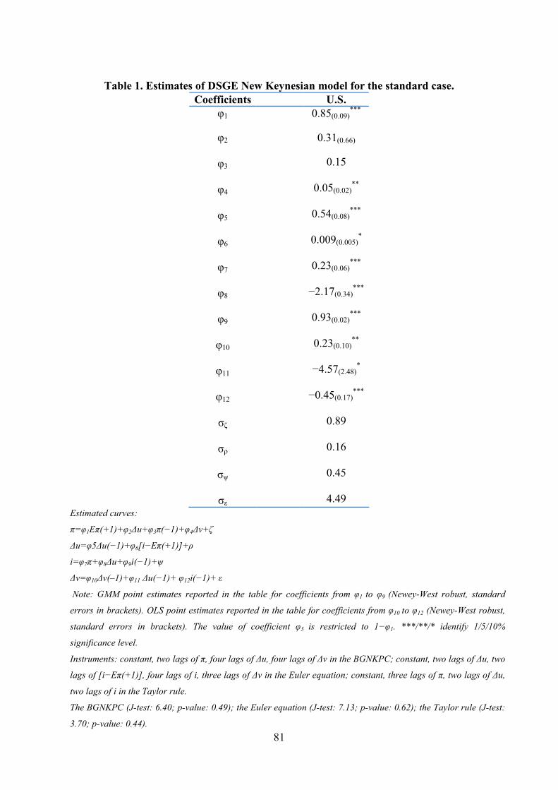
81
Table 1. Estimates of DSGE New Keynesian model for the standard case.
Coefficients U.S.
1 0.85(0.09)***
2
3
4
5
6
7
8
9
10
11
12
0.31(0.66)
0.15
0.05(0.02)**
0.54(0.08)***
0.009(0.005)*
0.23(0.06)***
−2.17(0.34)***
0.93(0.02)***
0.23(0.10)**
−4.57(2.48)*
−0.45(0.17)***
0.89
0.16
0.45
4.49
Estimated curves:
=1E(+1)+2u+3(−1)+4v+
u=5u(−1)+6[i−E(+1)]+
i=7+8u+9i(−1)+
v=10v(–1)+11 u(−1)+ 12i(−1)+
Note: GMM point estimates reported in the table for coefficients from 1 to 9 (Newey-West robust, standard
errors in brackets). OLS point estimates reported in the table for coefficients from 10 to 12 (Newey-West robust,
standard errors in brackets). The value of coefficient 3 is restricted to 1−1. ***/**/* identify 1/5/10%
significance level.
Instruments: constant, two lags of , four lags of u, four lags of v in the BGNKPC; constant, two lags of u, two
lags of [i−E(+1)], four lags of i, three lags of v in the Euler equation; constant, three lags of , two lags of u,
two lags of i in the Taylor rule.
The BGNKPC (J-test: 6.40; p-value: 0.49); the Euler equation (J-test: 7.13; p-value: 0.62); the Taylor rule (J-test:
3.70; p-value: 0.44).
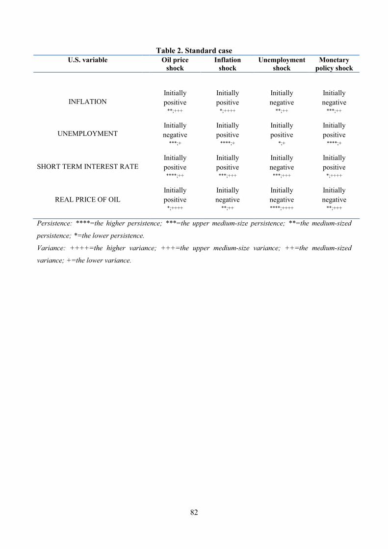
82
Table 2. Standard case
U.S. variable Oil price
shock
Inflation
shock
Unemployment
shock
Monetary
policy shock
INFLATION
Initially
positive **;+++
Initially
positive *;++++
Initially
negative **;++
Initially
negative ***;++
UNEMPLOYMENT
SHORT TERM INTEREST RATE
REAL PRICE OF OIL
Initially
negative ***;+
Initially
positive ****;++
Initially
positive *;++++
Initially
positive ****;+
Initially
positive ***;+++
Initially
negative **;++
Initially
positive *;+
Initially
negative***;+++
Initially
negative ****;++++
Initially
positive ****;+
Initially
positive*;++++
Initially
negative **;+++
Persistence: ****=the higher persistence; ***=the upper medium-size persistence; **=the medium-sized
persistence; *=the lower persistence.
Variance: ++++=the higher variance; +++=the upper medium-size variance; ++=the medium-sized
variance; +=the lower variance.
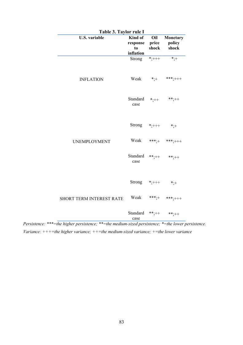
83
Table 3. Taylor rule I
U.S. variable Kind of
response
to
inflation
Oil
price
shock
Monetary
policy
shock
INFLATION
UNEMPLOYMENT
SHORT TERM INTEREST RATE
Strong
Weak
Standard
case
Strong
Weak
Standard
case
Strong
Weak
Standard
case
*;+++
*;+
*;++
*;+++
***;+
**;++
*;+++
***;+
**;++
*;+
***;+++
**;++
*;+
***;+++
**;++
*;+
***;+++
**;++
Persistence: ***=the higher persistence; **=the medium-sized persistence; *=the lower persistence.
Variance: +++=the higher variance; ++=the medium-sized variance; +=the lower variance
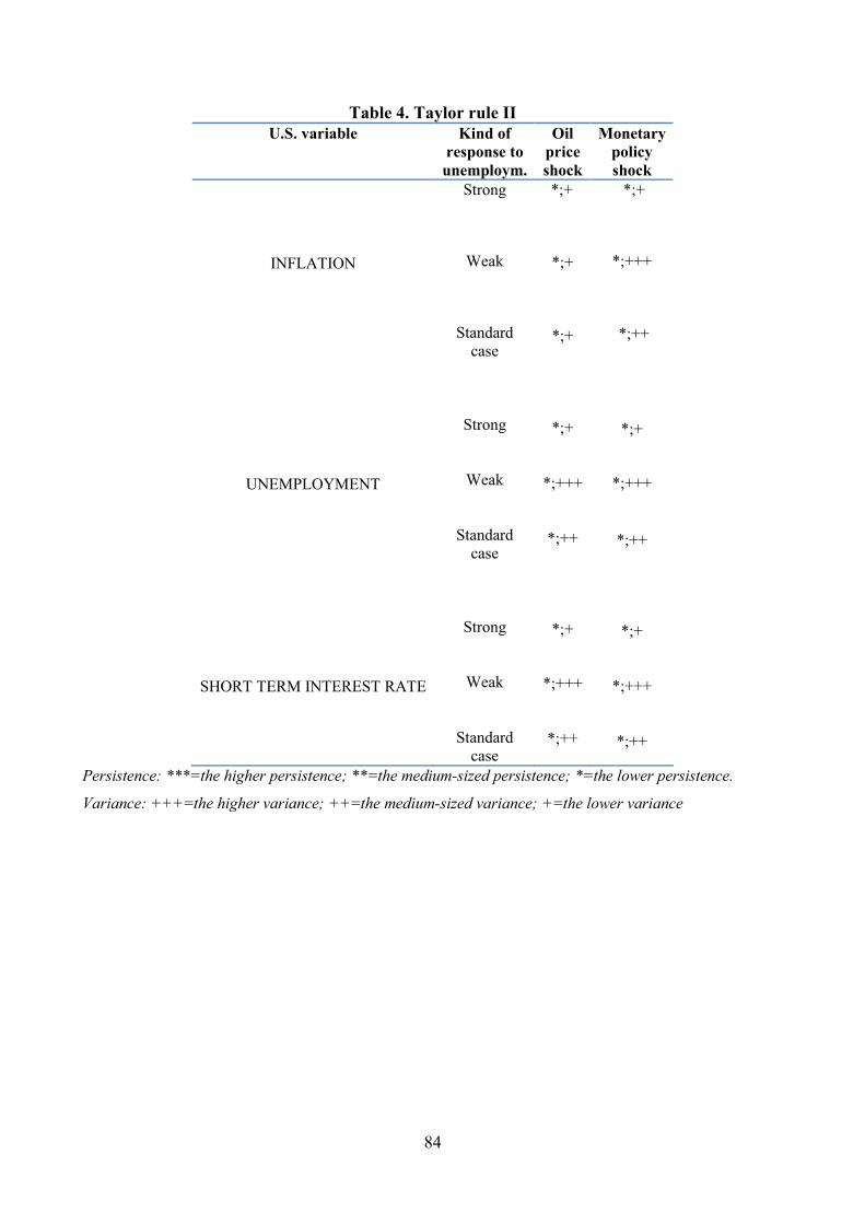
84
Table 4. Taylor rule II
U.S. variable Kind of
response to
unemploym.
Oil
price
shock
Monetary
policy
shock
INFLATION
UNEMPLOYMENT
SHORT TERM INTEREST RATE
Strong
Weak
Standard
case
Strong
Weak
Standard
case
Strong
Weak
Standard
case
*;+
*;+
*;+
*;+
*;+++
*;++
*;+
*;+++
*;++
*;+
*;+++
*;++
*;+
*;+++
*;++
*;+
*;+++
*;++
Persistence: ***=the higher persistence; **=the medium-sized persistence; *=the lower persistence.
Variance: +++=the higher variance; ++=the medium-sized variance; +=the lower variance
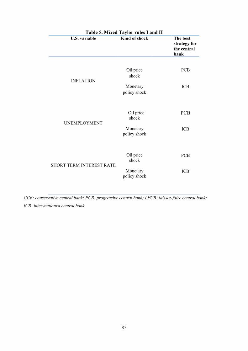
85
Table 5. Mixed Taylor rules I and II
U.S. variable Kind of shock The best
strategy for
the central
bank
INFLATION
UNEMPLOYMENT
SHORT TERM INTEREST RATE
Oil price
shock
Monetary
policy shock
Oil price
shock
Monetary
policy shock
Oil price
shock
Monetary
policy shock
PCB
ICB
PCB
ICB
PCB
ICB
CCB: conservative central bank; PCB: progressive central bank; LFCB: laissez-faire central bank;
ICB: interventionist central bank.
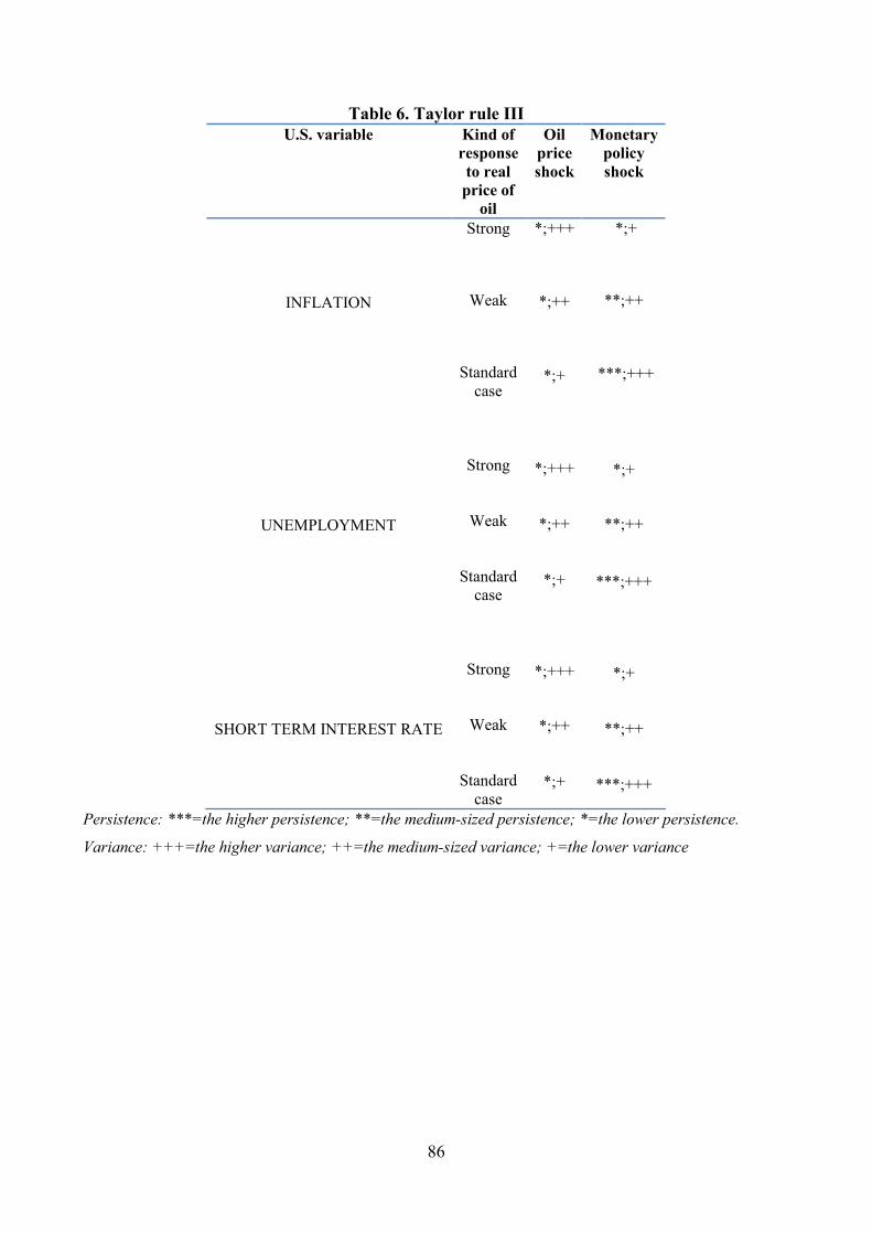
86
Table 6. Taylor rule III
U.S. variable Kind of
response
to real
price of
oil
Oil
price
shock
Monetary
policy
shock
INFLATION
UNEMPLOYMENT
SHORT TERM INTEREST RATE
Strong
Weak
Standard
case
Strong
Weak
Standard
case
Strong
Weak
Standard
case
*;+++
*;++
*;+
*;+++
*;++
*;+
*;+++
*;++
*;+
*;+
**;++
***;+++
*;+
**;++
***;+++
*;+
**;++
***;+++
Persistence: ***=the higher persistence; **=the medium-sized persistence; *=the lower persistence.
Variance: +++=the higher variance; ++=the medium-sized variance; +=the lower variance
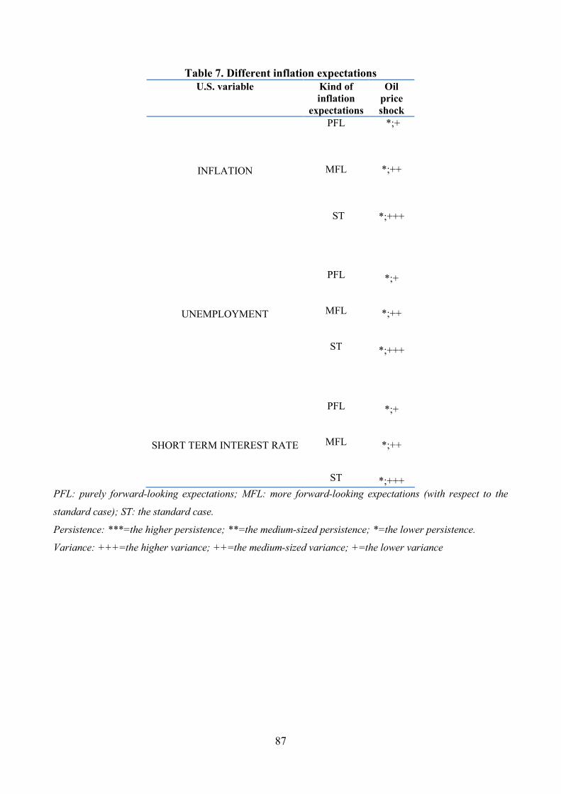
87
Table 7. Different inflation expectations
U.S. variable Kind of
inflation
expectations
Oil
price
shock
INFLATION
UNEMPLOYMENT
SHORT TERM INTEREST RATE
PFL
MFL
ST
PFL
MFL
ST
PFL
MFL
ST
*;+
*;++
*;+++
*;+
*;++
*;+++
*;+
*;++
*;+++
PFL: purely forward-looking expectations; MFL: more forward-looking expectations (with respect to the
standard case); ST: the standard case.
Persistence: ***=the higher persistence; **=the medium-sized persistence; *=the lower persistence.
Variance: +++=the higher variance; ++=the medium-sized variance; +=the lower variance
88
Data appendix
The data used come from: a)OECD Economic Outlook for GDP deflator; b)OECD Main
Economic Indicator for PPI , short term interest rate and real effective exchange rate; c)OECD
Labour Force Survey for standardised unemployment rate.
We define the variables of the equations (1)-(4) in the following way:
Inflation [(-1) and E(+1)]: for inflation we use the annualized percent change in the
GDP price deflator.
= [GDP −GDP(−1)] / GDP(−1)·4·100
where GDP is gross domestic product price deflator.
For inflation at the time minus one, (−1), we consider the realized inflation at the
previous quarter.
For expected future inflation, E(+1), we consider the realized inflation at the next quarter.
Change in unemployment (u): we define the change in unemployment using the
percent standardised unemployment rate.
u = u – u(–1)
Percent change in the real price of oil (v): we define the percent change in the real
price of oil as the annualized percent change in the PPI relative to the GDP price deflator.
v = [(PPI/GDP) − (PPI(−1)/GDP(−1))] / (PPI(−1)/GDP(−1))·4·100
v: annualized percent change in the real price of oil.
PPI: producer price index.
GDP: gross domestic product price deflator.
Short term interest rate (i): annualized short term interest rate.
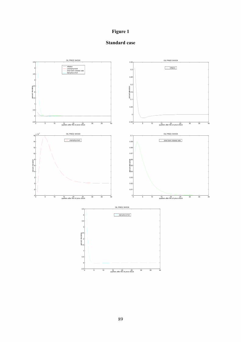
89
Figure 1
Standard case
0 5 10 15 20 25 30 35 40-0.5
0
0.5
1
1.5
2
2.5
3
3.5
4
4.5
quarters after the oil price shock
perc
ent
dev
iatio
n
OIL PRICE SHOCK
inflation
unemployment
short term interest rate
real price of oil
0 5 10 15 20 25 30 35 40-0.05
0
0.05
0.1
0.15
0.2
0.25
0.3
0.35
quarters after the oil price shock
perc
ent
devia
tio
n
OIL PRICE SHOCK
inflation
0 5 10 15 20 25 30 35 40-4
-2
0
2
4
6
8
10
12
14
16x 10
-4
quarters after the oil price shock
perc
ent
devia
tio
n
OIL PRICE SHOCK
unemployment
0 5 10 15 20 25 30 35 400
0.01
0.02
0.03
0.04
0.05
0.06
0.07
0.08
0.09
0.1
quarters after the oil price shock
perc
ent
devia
tio
n
OIL PRICE SHOCK
short term interest rate
0 5 10 15 20 25 30 35 40-0.5
0
0.5
1
1.5
2
2.5
3
3.5
4
4.5
quarters after the oil price shock
perc
ent
devia
tio
n
OIL PRICE SHOCK
real price of oil
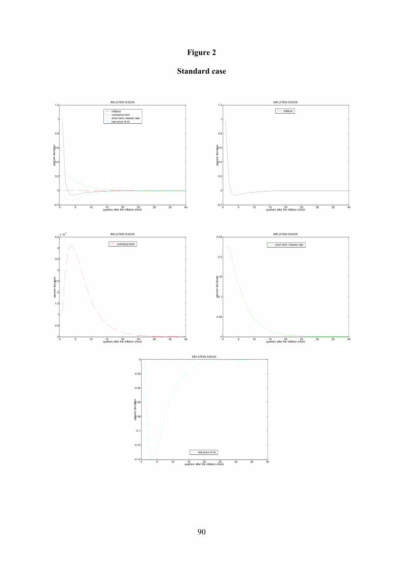
90
Figure 2
Standard case
0 5 10 15 20 25 30 35 40-0.2
0
0.2
0.4
0.6
0.8
1
1.2
quarters after the inflation shock
perc
ent
dev
iatio
n
INFLATION SHOCK
inflation
unemployment
short term interest rate
real price of oil
0 5 10 15 20 25 30 35 40-0.2
0
0.2
0.4
0.6
0.8
1
1.2
quarters after the inflation shock
perc
ent
dev
iatio
n
INFLATION SHOCK
inflation
0 5 10 15 20 25 30 35 400
0.5
1
1.5
2
2.5
3
3.5
4
4.5x 10
-3
quarters after the inflation shock
perc
ent
dev
iatio
n
INFLATION SHOCK
unemployment
0 5 10 15 20 25 30 35 400
0.05
0.1
0.15
0.2
0.25
quarters after the inflation shock
perc
ent
dev
iatio
n
INFLATION SHOCK
short term interest rate
0 5 10 15 20 25 30 35 40-0.14
-0.12
-0.1
-0.08
-0.06
-0.04
-0.02
0
quarters after the inflation shock
perc
ent
dev
iatio
n
INFLATION SHOCK
real price of oil
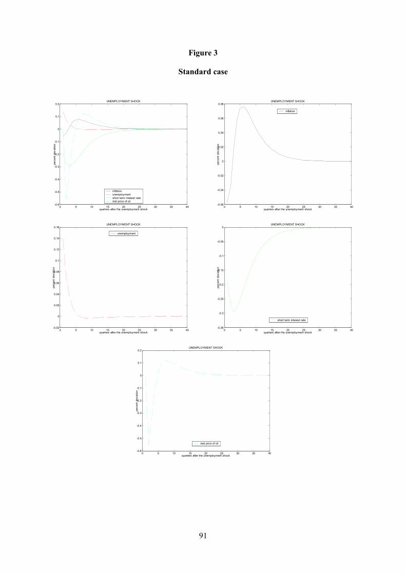
91
Figure 3
Standard case
0 5 10 15 20 25 30 35 40-0.6
-0.5
-0.4
-0.3
-0.2
-0.1
0
0.1
0.2
quarters after the unemployment shock
perc
ent
devia
tio
n
UNEMPLOYMENT SHOCK
inflation
unemployment
short term interest rate
real price of oil
0 5 10 15 20 25 30 35 40-0.06
-0.04
-0.02
0
0.02
0.04
0.06
0.08
quarters after the unemployment shock
perc
ent
devia
tio
n
UNEMPLOYMENT SHOCK
inflation
0 5 10 15 20 25 30 35 40-0.02
0
0.02
0.04
0.06
0.08
0.1
0.12
0.14
0.16
quarters after the unemployment shock
perc
ent
devia
tio
n
UNEMPLOYMENT SHOCK
unemployment
0 5 10 15 20 25 30 35 40-0.35
-0.3
-0.25
-0.2
-0.15
-0.1
-0.05
0
quarters after the unemployment shock
perc
ent
devia
tio
n
UNEMPLOYMENT SHOCK
short term interest rate
0 5 10 15 20 25 30 35 40-0.6
-0.5
-0.4
-0.3
-0.2
-0.1
0
0.1
0.2
quarters after the unemployment shock
perc
ent
devia
tio
n
UNEMPLOYMENT SHOCK
real price of oil
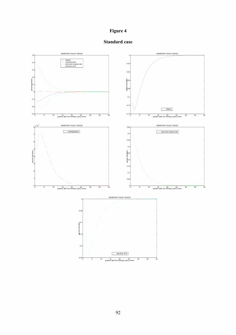
92
Figure 4
Standard case
0 5 10 15 20 25 30 35 40-0.3
-0.2
-0.1
0
0.1
0.2
0.3
0.4
0.5
quarters after the monetary policy shock
perc
ent
devia
tio
n
MONETARY POLICY SHOCK
inflation
unemployment
short term interest rate
real price of oil
0 5 10 15 20 25 30 35 40-0.14
-0.12
-0.1
-0.08
-0.06
-0.04
-0.02
0
quarters after the monetary policy shock
perc
ent
devia
tio
n
MONETARY POLICY SHOCK
inflation
0 5 10 15 20 25 30 35 400
1
2
3
4
5
6
7
8x 10
-3
quarters after the monetary policy shock
perc
ent
devia
tio
n
MONETARY POLICY SHOCK
unemployment
0 5 10 15 20 25 30 35 400
0.05
0.1
0.15
0.2
0.25
0.3
0.35
0.4
0.45
quarters after the monetary policy shock
perc
ent
devia
tio
nMONETARY POLICY SHOCK
short term interest rate
0 5 10 15 20 25 30 35 40-0.25
-0.2
-0.15
-0.1
-0.05
0
quarters after the monetary policy shock
perc
ent
devia
tio
n
MONETARY POLICY SHOCK
real price of oil
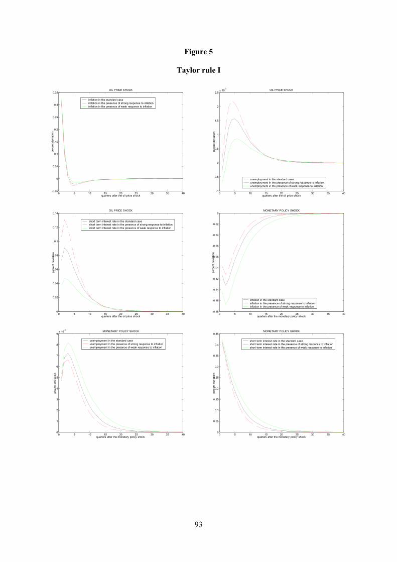
93
Figure 5
Taylor rule I
0 5 10 15 20 25 30 35 40-0.05
0
0.05
0.1
0.15
0.2
0.25
0.3
0.35
quarters after the oil price shock
perc
ent
devia
tio
n
OIL PRICE SHOCK
inflation in the standard case
inflation in the presence of strong response to inflation
inflation in the presence of weak response to inflation
0 5 10 15 20 25 30 35 40-1
-0.5
0
0.5
1
1.5
2
2.5x 10
-3
quarters after the oil price shock
perc
ent
devia
tio
n
OIL PRICE SHOCK
unemployment in the standard case
unemployment in the presence of strong response to inflation
unemployment in the presence of weak response to inflation
0 5 10 15 20 25 30 35 400
0.02
0.04
0.06
0.08
0.1
0.12
0.14
quarters after the oil price shock
perc
ent
devia
tio
n
OIL PRICE SHOCK
short term interest rate in the standard case
short term interest rate in the presence of strong response to inflation
short term interest rate in the presence of weak response to inflation
0 5 10 15 20 25 30 35 40-0.18
-0.16
-0.14
-0.12
-0.1
-0.08
-0.06
-0.04
-0.02
0
quarters after the monetary policy shock
perc
ent
devia
tio
nMONETARY POLICY SHOCK
inflation in the standard case
inflation in the presence of strong response to inflation
inflation in the presence of weak response to inflation
0 5 10 15 20 25 30 35 400
1
2
3
4
5
6
7
8
9x 10
-3
quarters after the monetary policy shock
perc
ent
devia
tio
n
MONETARY POLICY SHOCK
unemployment in the standard case
unemployment in the presence of strong response to inflation
unemployment in the presence of weak response to inflation
0 5 10 15 20 25 30 35 400
0.05
0.1
0.15
0.2
0.25
0.3
0.35
0.4
0.45
quarters after the monetary policy shock
perc
ent
devia
tio
n
MONETARY POLICY SHOCK
short term interest rate in the standard case
short term interest rate in the presence of strong response to inflation
short term interest rate in the presence of weak response to inflation
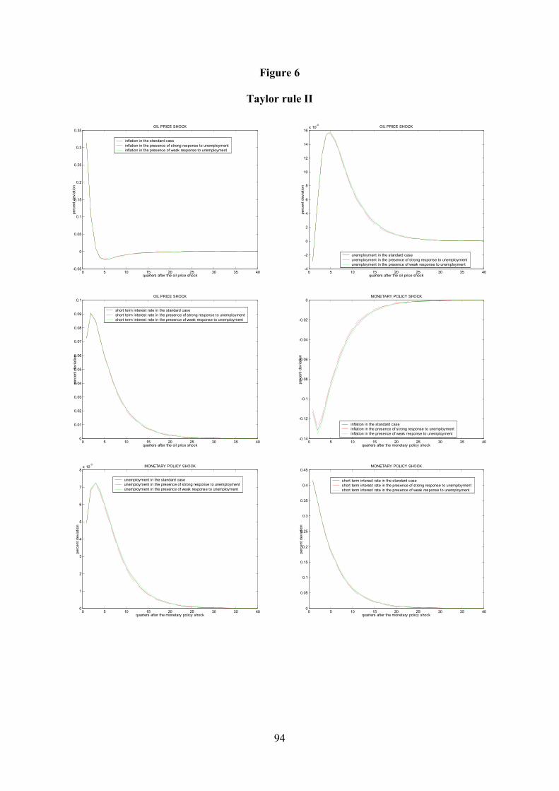
94
Figure 6
Taylor rule II
0 5 10 15 20 25 30 35 40-0.05
0
0.05
0.1
0.15
0.2
0.25
0.3
0.35
quarters after the oil price shock
perc
ent
devia
tio
n
OIL PRICE SHOCK
inflation in the standard case
inflation in the presence of strong response to unemployment
inflation in the presence of weak response to unemployment
0 5 10 15 20 25 30 35 40-4
-2
0
2
4
6
8
10
12
14
16x 10
-4
quarters after the oil price shock
perc
ent
devia
tio
n
OIL PRICE SHOCK
unemployment in the standard case
unemployment in the presence of strong response to unemployment
unemployment in the presence of weak response to unemployment
0 5 10 15 20 25 30 35 400
0.01
0.02
0.03
0.04
0.05
0.06
0.07
0.08
0.09
0.1
quarters after the oil price shock
perc
ent
devia
tio
n
OIL PRICE SHOCK
short term interest rate in the standard case
short term interest rate in the presence of strong response to unemployment
short term interest rate in the presence of weak response to unemployment
0 5 10 15 20 25 30 35 40-0.14
-0.12
-0.1
-0.08
-0.06
-0.04
-0.02
0
quarters after the monetary policy shock
perc
ent
devia
tio
nMONETARY POLICY SHOCK
inflation in the standard case
inflation in the presence of strong response to unemployment
inflation in the presence of weak response to unemployment
0 5 10 15 20 25 30 35 400
1
2
3
4
5
6
7
8x 10
-3
quarters after the monetary policy shock
perc
ent
devia
tio
n
MONETARY POLICY SHOCK
unemployment in the standard case
unemployment in the presence of strong response to unemployment
unemployment in the presence of weak response to unemployment
0 5 10 15 20 25 30 35 400
0.05
0.1
0.15
0.2
0.25
0.3
0.35
0.4
0.45
quarters after the monetary policy shock
perc
ent
devia
tio
n
MONETARY POLICY SHOCK
short term interest rate in the standard case
short term interest rate in the presence of strong response to unemployment
short term interest rate in the presence of weak response to unemployment
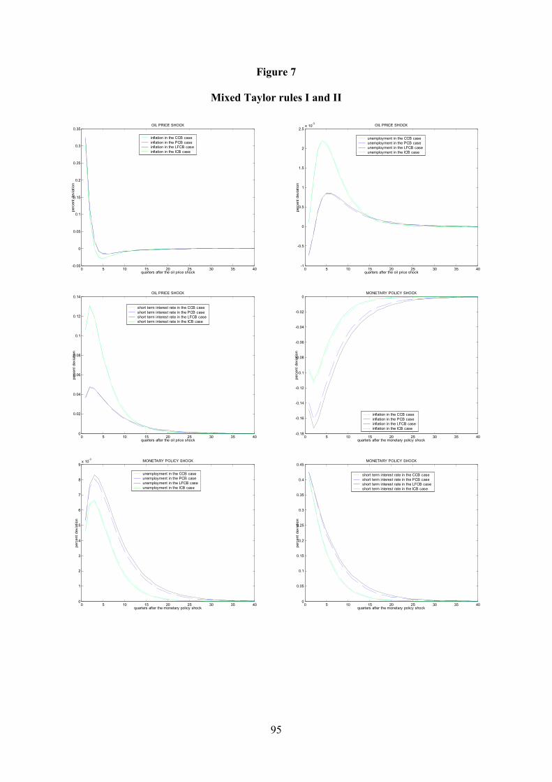
95
Figure 7
Mixed Taylor rules I and II
0 5 10 15 20 25 30 35 40-0.05
0
0.05
0.1
0.15
0.2
0.25
0.3
0.35
quarters after the oil price shock
perc
ent
devia
tio
n
OIL PRICE SHOCK
inflation in the CCB case
inflation in the PCB case
inflation in the LFCB case
inflation in the ICB case
0 5 10 15 20 25 30 35 40-1
-0.5
0
0.5
1
1.5
2
2.5x 10
-3
quarters after the oil price shock
perc
ent
devia
tio
n
OIL PRICE SHOCK
unemployment in the CCB case
unemployment in the PCB case
unemployment in the LFCB case
unemployment in the ICB case
0 5 10 15 20 25 30 35 400
0.02
0.04
0.06
0.08
0.1
0.12
0.14
quarters after the oil price shock
perc
ent
devia
tio
n
OIL PRICE SHOCK
short term interest rate in the CCB case
short term interest rate in the PCB case
short term interest rate in the LFCB case
short term interest rate in the ICB case
0 5 10 15 20 25 30 35 40-0.18
-0.16
-0.14
-0.12
-0.1
-0.08
-0.06
-0.04
-0.02
0
quarters after the monetary policy shock
perc
ent
devia
tio
nMONETARY POLICY SHOCK
inflation in the CCB case
inflation in the PCB case
inflation in the LFCB case
inflation in the ICB case
0 5 10 15 20 25 30 35 400
1
2
3
4
5
6
7
8
9x 10
-3
quarters after the monetary policy shock
perc
ent
devia
tio
n
MONETARY POLICY SHOCK
unemployment in the CCB case
unemployment in the PCB case
unemployment in the LFCB case
unemployment in the ICB case
0 5 10 15 20 25 30 35 400
0.05
0.1
0.15
0.2
0.25
0.3
0.35
0.4
0.45
quarters after the monetary policy shock
perc
ent
devia
tio
n
MONETARY POLICY SHOCK
short term interest rate in the CCB case
short term interest rate in the PCB case
short term interest rate in the LFCB case
short term interest rate in the ICB case
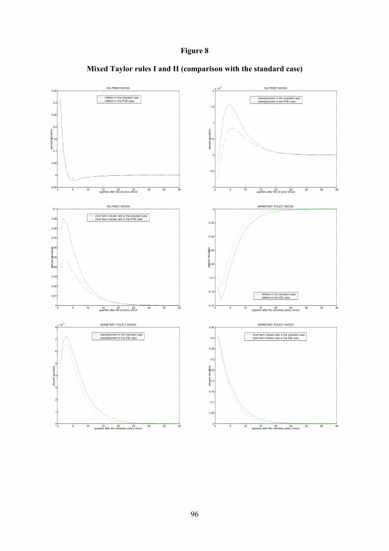
96
Figure 8
Mixed Taylor rules I and II (comparison with the standard case)
0 5 10 15 20 25 30 35 40-0.05
0
0.05
0.1
0.15
0.2
0.25
0.3
0.35
quarters after the oil price shock
perc
ent
devia
tio
n
OIL PRICE SHOCK
inflation in the standard case
inflation in the PCB case
0 5 10 15 20 25 30 35 40-1
-0.5
0
0.5
1
1.5
2x 10
-3
quarters after the oil price shock
perc
ent
devia
tio
n
OIL PRICE SHOCK
unemployment in the standard case
unemployment in the PCB case
0 5 10 15 20 25 30 35 400
0.01
0.02
0.03
0.04
0.05
0.06
0.07
0.08
0.09
0.1
quarters after the oil price shock
perc
ent
devia
tio
n
OIL PRICE SHOCK
short term interest rate in the standard case
short term interest rate in the PCB case
0 5 10 15 20 25 30 35 40-0.14
-0.12
-0.1
-0.08
-0.06
-0.04
-0.02
0
quarters after the monetary policy shock
perc
ent
devia
tio
nMONETARY POLICY SHOCK
inflation in the standard case
inflation in the ICB case
0 5 10 15 20 25 30 35 400
1
2
3
4
5
6
7
8x 10
-3
quarters after the monetary policy shock
perc
ent
devia
tio
n
MONETARY POLICY SHOCK
unemployment in the standard case
unemployment in the ICB case
0 5 10 15 20 25 30 35 400
0.05
0.1
0.15
0.2
0.25
0.3
0.35
0.4
0.45
quarters after the monetary policy shock
perc
ent
devia
tio
n
MONETARY POLICY SHOCK
short term interest rate in the standard case
short term interest rate in the ICB case
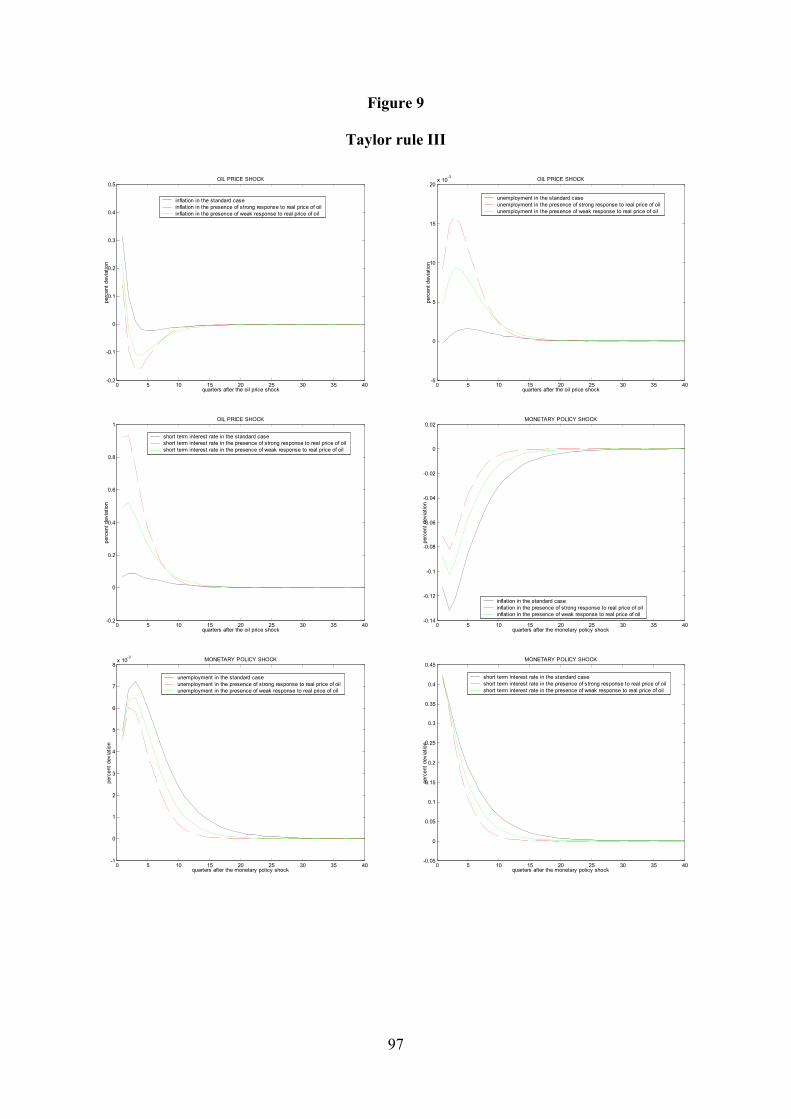
97
Figure 9
Taylor rule III
0 5 10 15 20 25 30 35 40-0.2
-0.1
0
0.1
0.2
0.3
0.4
0.5
quarters after the oil price shock
perc
ent
devia
tio
n
OIL PRICE SHOCK
inflation in the standard case
inflation in the presence of strong response to real price of oil
inflation in the presence of weak response to real price of oil
0 5 10 15 20 25 30 35 40-5
0
5
10
15
20x 10
-3
quarters after the oil price shock
perc
ent
devia
tio
n
OIL PRICE SHOCK
unemployment in the standard case
unemployment in the presence of strong response to real price of oil
unemployment in the presence of weak response to real price of oil
0 5 10 15 20 25 30 35 40-0.2
0
0.2
0.4
0.6
0.8
1
quarters after the oil price shock
perc
ent
devia
tio
n
OIL PRICE SHOCK
short term interest rate in the standard case
short term interest rate in the presence of strong response to real price of oil
short term interest rate in the presence of weak response to real price of oil
0 5 10 15 20 25 30 35 40-0.14
-0.12
-0.1
-0.08
-0.06
-0.04
-0.02
0
0.02
quarters after the monetary policy shock
perc
ent
devia
tio
nMONETARY POLICY SHOCK
inflation in the standard case
inflation in the presence of strong response to real price of oil
inflation in the presence of weak response to real price of oil
0 5 10 15 20 25 30 35 40-1
0
1
2
3
4
5
6
7
8x 10
-3
quarters after the monetary policy shock
perc
ent
devia
tio
n
MONETARY POLICY SHOCK
unemployment in the standard case
unemployment in the presence of strong response to real price of oil
unemployment in the presence of weak response to real price of oil
0 5 10 15 20 25 30 35 40-0.05
0
0.05
0.1
0.15
0.2
0.25
0.3
0.35
0.4
0.45
quarters after the monetary policy shock
perc
ent
devia
tio
n
MONETARY POLICY SHOCK
short term interest rate in the standard case
short term interest rate in the presence of strong response to real price of oil
short term interest rate in the presence of weak response to real price of oil
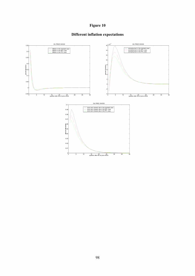
98
Figure 10
Different inflation expectations
0 5 10 15 20 25 30 35 40-0.05
0
0.05
0.1
0.15
0.2
0.25
0.3
0.35
quarters after the oil price shock
perc
ent
devia
tio
n
OIL PRICE SHOCK
inflation in the standard case
inflation in the MFL case
inflation in the PFL case
0 5 10 15 20 25 30 35 40-4
-2
0
2
4
6
8
10
12
14
16x 10
-4
quarters after the oil price shock
perc
ent
devia
tio
n
OIL PRICE SHOCK
unemployment in the standard case
unemployment in the MFL case
unemployment in the PFL case
0 5 10 15 20 25 30 35 400
0.01
0.02
0.03
0.04
0.05
0.06
0.07
0.08
0.09
0.1
quarters after the oil price shock
perc
ent
devia
tio
n
OIL PRICE SHOCK
short term interest rate in the standard case
short term interest rate in the MFL case
short term interest rate in the PFL case