Embed Size (px)
Citation preview

UNIVERSITA’ DI PADOVA FACOLTA’ DI INGEGNERIA
Dipartimento di Ingegneria dell’Informazione
Scuola di Dottorato di Ricerca in Ingegneria dell’Informazione
Indirizzo: Bioingegneria
Ciclo XX
PET PARAMETRIC IMAGING OF ACETYLCHOLINE ESTERASE ACTIVITY
WITHOUT ARTERIAL BLOOD SAMPLING IN NORMAL SUBJECTS AND
PATIENTS WITH NEURODEGENERATIVE DISEASE
Dottorando: Ioana Florea
Supervisori: Ch.mo Prof. Claudio Cobelli
Ch.mo Prof. Maria Carla Gilardi
Direttore della Scuola: Ch.mo Prof. Silvano Pupolin
Gennaio 2008

ii

To my family
"From the brain and the brain alone arise our pleasures, joys, laughter
and jests, as well as our sorrows, pains and griefs"
(Hippocrates)

iv

Contents
Contents ................................................................................................. v
List of Figures ....................................................................................... vii
List of Tables ........................................................................................ xiii
Summary ............................................................................................... xv
English ................................................................................................ xv
Italiano ............................................................................................... xix
Chapter 1 ............................................................................................... 1
Introduction ........................................................................................... 1
Chapter 2 ............................................................................................... 7
Cholinergic System ................................................................................ 7
2.1. Biosynthesis and Metabolism of ACh. ............................................ 8
2.2. Acetylcholinesterase and the Termination of Acetylcholine Action. 10
2.3. Pharmacology .............................................................................. 12
Cholinergic System in Alzheimer Disease. .................................... 14
2.4. PET Tracer: 11C-MP4A. ................................................................ 15
Chapter 3 ............................................................................................. 19
Image Acquisition and Processing ...................................................... 19
3.1. Subjects ...................................................................................... 19
3.2. 11C-MP4A PET ............................................................................. 19
3.3. Automatic generation of ROIs ...................................................... 20

Contents
vi
Chapter 4 .............................................................................................. 25
Models and Methods for 11C-MP4A Quantification .............................. 25
4.1. RLS (Reference Tissue Based Linear Least Square Method) ........... 29
4.2. RRE (Reference Ratio Exponential Approach) ................................ 31
4.3. RRE_BF model (Reference Ratio Exponential based on Basis
Function Approach) ............................................................................. 34
4.4. R-NLLS (Reference Tissue based Non Linear Least Square Method)
………………………………………………………………………………………….37
4.5. MAP (Reference Tissue based Maximum a Posteriori Parameter
Estimation) ......................................................................................... 38
4.6. Parametric Images Processing ...................................................... 40
Chapter 5 .............................................................................................. 43
Results .................................................................................................. 43
5.1. RLS results and discussion .......................................................... 43
5.2. RRE results and discussion .......................................................... 48
5.3. RRE_BF results and discussion. ................................................... 53
5.4. R-NLLS results and discussion. .................................................... 59
5.5. MAP results and discussion. ......................................................... 62
Chapter 6 .............................................................................................. 67
MP4A Functional Parametric Images: Assessment and Models
Comparison. .......................................................................................... 67
Chapter 7 .............................................................................................. 75
Discussion ............................................................................................. 75
Chapter 8 .............................................................................................. 79
Conclusions .......................................................................................... 79
Bibliography .......................................................................................... 83
Acknowledgments ................................................................................. 91

List of Figures
FIGURE 2.1 Acetylcholine system: network of cholinergic neurons [38] . . 7
FIGURE 2.2 Acetylcholine metabolism in cholinergic nerve terminals. The
synthesis of acetylcholine from choline and acetyl CoA requires choline
acetyltransferase. Acetyl CoA is derived from pyruvate generated by
glycolysis, while choline is transported into the terminals via a Na+-
dependent transporter. After release, acetylcholine is rapidly metabolized
by acetylcholinesterase and choline is transported back into the terminal
[40]. ....................................................................................................... 10
FIGURE 2.3 Distribution of the cholinergic receptors [24]. ..................... 13
FIGURE 2.4 Types and structure of cholinergic receptors: nicotinic (Panel
A) and muscarinic (Panel B) receptors [38]……………………………………..13
FIGURE 2.5 Total and metabolite-corrected radioactivity of the arterial
plasma in a subject after intravenous injection of 11C-MP4A. Time 0=start
of intravenous tracer infusion. Inset: Semilogarithmic plot of the
metabolite-corrected radioactivity up to 15 min after intravenous injection
of 11C-MP4A and a fitted curve up to 40 min [8]….…………………………..16
FIGURE 2.6 Time-activity curves in the cerebral (temporal) cortex,
thalamus and cerebellar cortex in a subject after intravenous injection of 11C-MP4A [8]. .. ………………………………………………………………………...17

List of Figures
FIGURE 2.7 Average images of controls (C) and AD patients (AD) with
stereotactic normalization. Coronal slices (perpendicular to the AC–PC
line) are shown, starting at the AC and progressing in 2 mm steps
caudally (distance from AC shown in the middle of the figure). MRI images
are shown on top, 11C-MP4A PETscaled to 65% of maximum brain activity
at bottom. The anteromedial and anterolateral parts of the nbM are
marked by a pink arrow (the posterior part is located just below the
putamen with its very high activity and cannot be separated). The
amygdalae are marked by an orange arrow. Please note the progression of
the distance between the left and right optic tract from 0 to 8 mm caudal
to the AC. This serves as a landmark to compare the anatomical site with
the histochemical studies (Hedreen et al., 1984; Mesulam and Geula,
1988b). In AD (bottom row), AChE activity was reduced in cortex and
amygdala, but not in nbM.[19]. .... ………………………………………………..18
FIGURE 3.1. Examples of mask ROI generation with Marina software:
region with low enzyme activity like temporal lobe (TE) and HP in Panel B
and respectively Panel A, and moderate enzyme expression as and TH in
Panel C. From left to right, in each panel are represented coronal, sagital
and transversal view. .............................................................................. 22
FIGURE 3.2 11C-MP4A average 1-10 "early" image of controls (NC) middle
line and AD patients (AD) bottom line normalized to stereotactic space and
corregistered to the single-subject (MRI) canonical template of SPM (top
line) shown in each panel. Coronal view-Panel A and transversal view –
Panel…………………....……………………………………………………………….23
FIGURE 3.3 11C-MP4A time activity curves e.g. in NC Image Processing . 24
FIGURE 3.4 The flowchart of 4D 11C-PET images processing at TAC_ROI
level ....................................................................................................... 24
viii
List of Figures
FIGURE 4.1 The two-tissue three-rate constant compartmental model of
11C-MP4A in brain region having low or intermediate AChE activity. Cp is
the unmetabolized free tracer concentration curve in plasma, C1 the 11C-
MP4A tracer concentration in tissue, C2 the 11C-MP4OH metabolite
concentration in tissue, K1 [ml/ml/min] the rate of tracer inflow into the
brain, k2 [min-1] the rate of unmetabolized tracer washout, and k3 [min-1]
the rate of tracer hydrolysis by AChE. .................................................... 26
FIGURE 4.2 The one-tissue one-rate constant compartmental model of 11C-MP4A in brain region having high AChE activity. Cp is the
unmetabolized free tracer concentration curve in plasma, CR the 11C-MP4A
tracer concentration in the target tissue, K1R [ml/ml/min] the joint rate
constant of both tracer inflow into the tissue brain and tracer hydrolysis
activity. ................................................................................................. 27
FIGURE 4.3 The flowchart of 4D 11C-MP4A PET images processing at
pixel-by-pixel level ................................................................................. 41 FIGURE 5.1 Average of normalized and co-registered parametric image of
k3 obtained with RLS mathematical procedure for both groups of subjects:
NC upper line and AD bottom line in Panel A and Panel B. Image scale: [0,
0.4] min-1. ............................................................................................. 46
FIGURE 5.2 RLS k3 estimates at pixel-by-pixel (pxp) level (top panel),
TAC_ROI level (middle panel) and comparison pixel vs TAC_ROI estimates
(bottom panel). ...................................................................................... 47
FIGURE 5.3 Average of normalized and co-registered parametric image of
k3 obtained with RRE mathematical procedure for both groups of subjects:
NC upper line and AD bottom line in panel A and panel B. Image scale: [0,
0.4] min-1. ............................................................................................ 49
ix

List of Figures
FIGURE 5.4 RRE k3 estimates at pixel-by-pixel (pxp) level (top panel),
TAC_ROI level (middle panel) and comparison pixel vs TAC_ROI estimates
(bottom panel). ....................................................................................... 50
FIGURE 5.5 Average of normalized and co-registered parametric image of
k3 obtained with RRE mathematical procedure not corrected (RRE) and
corrected with the threshold (RRE_t) for both groups of subjects: NC
(RRE_NC, RRE_t_NC) left part of the panel and AD (RRE_AD, RRE_t_AD)
located on the right part of the panel. Images scale: [0, 0.4] min-1. .......... 52
FIGURE 5.6 Average of normalized and co-registered parametric image of
k3 obtained with RRE_BF mathematical procedure for both groups of
subjects: NC upper line and AD bottom line in each panel considering the
assumption on K index: C1 in panel A, C2 in panel B and C3 in panel C.
Images scale: [0, 0.4] min-1. .................................................................... 57
FIGURE 5.7 RRE_BF k3 estimates at pixel-by-pixel level in NC vs AD when
consider the different assumption for K (panel A) and the variation of the
mean estimates within subject group (NC and respectively AD group) in
Panel B. ................................................................................................. 58
FIGURE 5.8 Average of normalized and co-registered parametric image of
k3 obtained with R-NLLS mathematical procedure for both groups of
subjects: NC upper line and AD bottom line in panel A and panel B. Image
scale: [0, 0.4] min-1. ................................................................................ 60
FIGURE 5.9 R-NLLS k3 estimates at pixel-by-pixel level (top panel),
TAC_ROI level (middle panel) and comparison pixel vs TAC_ROI estimates
(bottom panel). ....................................................................................... 61
FIGURE 5.10 Average of normalized and co-registered parametric image of
k3 obtained with MAP mathematical procedure for both groups of subjects:
NC upper line and AD bottom line in Panel A and Panel B. Image scale: [0,
0.4] min-1. .............................................................................................. 65
x

List of Figures
FIGURE 5.11 MAP k3 estimates at pixel-by-pixel (pxp) level (top panel),
TAC_ROI level (middle panel) and comparison pixel vs TAC_ROI estimates
(bottom panel). ...................................................................................... 66
FIGURE 6.1 k3 mean parametric images for both groups of subjects (NC
on the left and AD on the right part of each panel) obtained with all
described techniques: RLS, RRE, RRE_BF, R-NLLS, and MAP. ............... 70
FIGURE 6.2 Mean ± SD k3 obtained with all applied mathematical
procedures at pixel level in both NC and AD groups. The red line
represents the considered “true” NC k3 value for each considered brain
area. ...................................................................................................... 73
xi

List of Figures
xii

List of Tables
TABLE 5.1 RLS k3 indexes obtained at pixel-by-pixel level and TAC_ROI
level in brain area with low enzyme activity (neocortex) and low to
moderate (HP, R, I) and moderate (TH) enzyme expression in both group of
subjects and the respective p value. ....................................................... 44
TABLE 5.2 RRE k3 indexes obtained at pixel-by-pixel level and TAC_ROI
level in brain area with low enzyme activity (neocortex) and low to
moderate (HP, R, I) and moderate (TH) enzyme expression in both group of
subjects and the respective p value. ....................................................... 48
TABLE 5.3 RRE k3 indexes obtained at pixel-by-pixel level before (RRE)
and after threshold correction (RRE_t) in brain area with low enzyme
activity (neocortex) and low to moderate (HP, R, I) and moderate (TH)
enzyme expression in both group of subjects and the respective p value. 51
TABLE 5.4 RRE_BF mean k3 indexes obtained at pixel-by-pixel level
(considering the three assumption of range (b) and the number of basis
function (NBF)) in brain areas with low enzymatic activity (neocortex) and
low to moderate (HP,R,I) and moderate (TH) enzyme expression in both
group of subjects and the respective p value. ......................................... 55
TABLE 5.5 R-NLLS k3 indexes obtained at pixel-by-pixel level in brain
area with low enzyme activity (neocortex) and low to moderate (HP, R, I)
and moderate (TH) enzyme expression in both group of subjects and the
respective p value. ................................................................................. 59

List of Tables
xiv
TABLE 5.6 MAP k3 indexes obtained at pixel-by-pixel and TAC_ROI level
in brain area with low enzyme activity (neocortex) and low to moderate
(HP, R, I) and moderate (TH) enzyme expression in both group of subjects
and the respective p value. ..................................................................... 63
TABLE 6.1 Mean ± SD regional values of k3 parameter extracted from the
parametric images obtained with different estimation approaches for both
groups participated at the study. * recalls that we considered reliable the
RRE estimated cleaned for the k2 threshold identified for each subject; **
remind that for basis function approach(RRE_BF) were considered more
reliable the result obtained with the assumption C1 for K: range from 0.05
to 0.5 and NBF=100………………………………………………………………….71
TABLE 6.2 Bias of the mean k3 estimates in NC obtained with all
mathematical procedures respect to the considered k3 “true” value. *
recalls that were considered reliable the RRE estimated cleaned for the k2
threshold identified for each subject; ** remind that for basis function
approach(RRE_BF) were considered more reliable the result obtained with
the assumption C1 for K: range from 0.05 to 0.5 and NBF=100……. ....... 72

Summary
Assessment of the integrity of the cortical cholinergic system is of primary
interest in dementia because of its crucial role for memory and attention.
The use of PET (Positron Emission Tomography) and tracers that are
hydrolysed specifically by acetylcholine esterase (AChE) permits
measurement and imaging of local AChE activity in humans. Carbon-11-
labelled N-methyl-4 piperidyl-acetate (11C-MP4A) is a PET tracer that is
highly specific for AChE and has kinetic properties that are favorable for
measuring cortical AChE activity. Kinetic analysis of these images
provides the quantification of AChE activity; the analysis can be
performed both at pixel and region of interest (ROI) level.
The standard method to estimate regional hydrolysis rate of 11C-
MP4A by AChE is to identify by nonlinear least squares (NLLS) the
parameter estimates of the model using the arterial concentration of tracer
as input function. However, the measurement of the arterial input
function is an invasive procedure for the patients and requires
considerable technical expertise, which may restrict widespread use of
this method in daily clinical practice. To overcome this drawback, in the
last years, different methods have been proposed for non-invasive
quantification of AChE activity at region of interest level: shape analysis,
firstly proposed by Koeppe et al.; reference tissue linear least squares
(RLS) proposed by Nagatsuka et al. (2001); reference ratio exponential
(RRE) approach proposed by Herholz and coworkers in 2001.
Nevertheless, only few attempts have been made in order to quantify no
invasively AChE activity at pixel level: Zundorf et al. in 2002 which
implemented a basis function approach (RRE_BF) to Herholz technique in

Summary
order to reduce unnecessary bias, while estimating the parameters of
interest. The methods available in literature, based on reference region
input, do not consider the reliability and the accuracy of all the parameter
estimates.
The purpose of this study is to propose and develop a Bayesian
method, based on maximum a posteriori information (MAP), to quantify 11C-MP4A activity at pixel level in patients with neurodegenerative
diseases and in normal subjects. The main goal is to accurately estimate
AChE activity in brain regions with low (neocortex) and moderate
(thalamus) enzymatic expression taking into account the reliability of all
estimates. Bayesian estimator allows to quantify model parameters
maximizing the conditional probability of data given parameters: it uses
information contained in the data, the so called a posteriori information
and consider also a priori probability information of all or some of the
parameters. In our study, a priori information is obtained for each subject
who participates at the study from a preliminary reference weighted non
linear least squares (R_NLLS) analysis implemented at ROI level. R_NLLS
analysis, as already confirmed by the literature, evidences a low inter-
region variability within subject of the parameter that characterize the
unmetabolized tracer washout from tissue to blood. Therefore, it can be
assumed that this parameter has a priori a Gaussian probability density
function with mean and standard deviation obtained from R_NLLS at ROI
level. This additional probabilistic information is used to estimate tracer
kinetic indexes at pixel level applying MAP procedure to PET dynamic
images.
Another intent of this work is to compare the performance of the
Bayesian estimator with the other few methods already propose in the
literature for AChE activity quantification implemented at pixel level. The
comparison between methods is based on the precision of estimates.
A new method for an automatic extraction of ROIs is also proposed
in this study. Automatic extraction is preferred to the often used manual
technique: first, because of the lack of subjects MRI scans that are usually
xvi

Summary
used as anatomical reference in identifying brain regions of interest;
second, in order to avoid errors sampling during a manual position of
ROIs on the dynamic or parametric 11C-MP4A PET images.
Bayesian method, as well as already published methods, is based on
the same compartmental model that describes tracer kinetics: reference
region described by one tissue-one rate constant, while the target tissue is
described by a two tissue compartment - three rate constant model. This
kinetic model is actually considered the best model to quantify 11C-MP4A
data. AChE activity is measured in terms of the rate constant for
hydrolysis of 11C-MP4A, k3. Striatum (basal ganglia) is chose as reference
structure to be used as input function for all models, because of its very
high AChE activity. All methods have been applied at both pixel and ROI
level (except for RRE_BF proposed only for pixel level). Only estimates with
good precision are accepted for the comparison study. The consistence of
estimates obtained by each mathematical approach for both analysis
levels is also investigated.
The automatic extraction of anatomical areas and the comparison
study of the different methodologies for AChE activity quantification at
pixel level confirm that in cortex area with low enzyme activity the models
have similar performance. However, for RRE and RRE_BF approaches
inaccurate estimates of the parameter that describes the unmetabolized
tracer washout from tissue to blood is observed. Thus, in order to have
only reliable estimates for these two methods, a threshold of inaccurate
parameter was calculated for each PET study and applied as acceptability
condition for estimates. Anyway, this correction does not improve RRE_BF
performance. However, from computational point of view, RLS linear
calculation is faster for pixel by pixel parameter estimation respect to non
linear quantification methods (R-NLLS, MAP) and the results are in good
agreement with published neocortex values.
On the contrary, RLS approach shows some difficulties in
estimating k3 index in area with moderate enzyme activity, such as
thalamus and brainstem. The use of Bayesian (MAP) estimator helps to
xvii

Summary
xviii
overcome these drawbacks and allows the quantification of AChE activity
in regions with moderate enzyme expression, like thalamus and
brainstem. At pixel level, this procedure presents results consistent with
the scientific literature. MAP technique is more time consuming respect to
the other methods because it implicates a previous analysis at ROI level in
order to obtain the a priori information, but improve the precision of
estimates. Actually, pixel and ROI estimates obtain applying the Bayesian
estimator are more similar respect to the ones obtained with published
methods.
In conclusion, MAP method is the best quantification approach, in
terms of precision and accuracy, for AChE activity in both area with low
and moderate enzyme expression. Pixel level estimates, even if it’s a
procedure more time consuming, are more reliable because conserve all
the information contained in the cortical map respect to the ROI approach
where loss of resolution is a major drawback.
An European project finalized to validate on a bigger dataset the
best method to be applied to 11C-MP4A/PET images is going to start soon.
Its aim will be the confirmation of the clinical applicability of the chosen
technique in the discrimination of different neurodegenerative pathologies
as AD, Lewy body dementia (DLB), mild cognitive impairment (MCI). MAP
procedure as well as another Bayesian method under development will be
taken into account. Simulation study based on real plasma input are
going to be considered for best method validation.

Sommario
La valutazione dell’integrità del sistema colinergico, considerato il suo
ruolo cruciale nei meccanismi cerebrali che regolano la memoria e
l’attenzione, è di grande interesse nelle malattie neurodegenerative come
la demenza.
L’utilizzo della PET (tomografia ad emissione di positroni) e dei
traccianti che sono idrolizzati in modo specifico dall’acetilcolinesterase
(AChE) permette di misurare l’attività enzimatica cerebrale in vivo
nell’uomo. In particolare, il N-metil-4 piperidil-acetato (MP4A) marcato con
carbonio 11 (11C) è un tracciante PET molto specifico per AChE ed ha delle
proprietà cinetiche che favoriscono lo studio dell’attività corticale
dell’AChE. Più precisamente, l’analisi quantitativa delle immagini
acquisite tramite PET e 11C-MP4A permette di stimare l’attività dell’AChE
in termini di velocità di metabolismo (per idrolisi) del 11C-MP4A; l’analisi
può essere effettuata al livello di pixel o al livello di regione di interesse
(ROI).
Il metodo standard per la stima dell’attività dell’AChE si basa
sull’uso dei minimi quadrati non lineari ed utilizza come funzione
d’ingresso la concentrazione plasmatica del tracciante. La misura della
concentrazione plasmatica, però, è invasiva, richiede un’ampia esperienza
tecnica e costituisce un fattore importante di limitazione all’uso
dell’indagine PET con 11C-MP4A nella pratica clinica di routine. Per
superare questo inconveniente, negli ultimi anni sono stati proposti vari
metodi per la quantificazione non invasiva dell’attività dell’AChE al livello
di ROI: la shape analisi (SA) proposta da Koeppe et al; il metodo a tessuto

Sommario
di riferimento proposto da Nagatsuka et al (2001) basato sui minimi
quadrati lineari (RLS); il metodo del quoziente esponenziale (RRE) proposto
da Herholz e collaboratori (2001). I tentativi di stima dell’attività
enzimatica al livello di pixel sono stati, invece, pochi tra cui il più
interessante è stato sviluppato e proposto da Zundorf e colleghi nel 2002
(RRE_BF). Comunque, tutti i metodi proposti per la quantificazione senza
funzione di ingresso arteriale non prendono in considerazione l’affidabilità
e l’accuratezza di tutti parametri stimati.
Uno degli obbiettivi di questo studio è di proporre e sviluppare
un nuovo metodo basato sull’utilizzo dello stimatore Bayesiano di
probabilità massima a posteriori (MAP) per la quantificazione non invasiva
al livello di pixel dell’attività enzimatica dell’AChE in individui normali e in
soggetti affetti da malattie neurodegenerative. Lo scopo principale è di
stimare in modo accurato e preciso l’attività dell’AChE in regioni cerebrali
con espressione enzimatica bassa (neocortex) e media (talamo)
considerando l’affidabilità di tutti parametri. Lo stimatore MAP utilizza sia
le informazioni contenute nei dati – le cosiddette informazioni a posteriori –
che le informazioni statistiche a priori disponibili su alcuni o tutti i
parametri incogniti. Nel corso di questo studio, le informazioni a priori
sono state ricavate per ogni soggetto che ha partecipato allo studio tramite
un’analisi preliminare a tessuto di riferimento basata sui minimi quadrati
non lineari (R_NLLS) implementata al livello di ROI. L’analisi R_NLLS,
come già confermato in letteratura, evidenzia una bassa variazione del
parametro che caratterizza l’eliminazione del tracciate non metabolizzato
dal tessuto nel sangue. Di conseguenza, questo parametro è stato assunto
avere una distribuzione di probabilità Gaussiana a priori, con media e
deviazione standard pari a quella ottenuta con R_NLLS al livello di ROI.
Questa informazione probabilistica addizionale costituisce l’informazione a
priori fornita allo stimatore MAP.
Un altro obbiettivo di questo studio è rappresentato dalla messa a
confronto e selezione del metodo più affidabile per la quantificazione
dell’attività corticale.
xx

Sommario
Per limitare il più possibile gli errori di posizionamento delle ROI
sulle immagini dinamiche e/o parametriche e limitare al contempo l’effetto
di volume parziale, si è fatto uso di un nuovo metodo automatico
disponibile in rete per la generazione di ROI.
Sia il metodo MAP che gli altri metodi considerati si basano sullo
stesso modello compartimentale a tessuto di riferimento (due
compartimenti tessutali e tre costanti di trasferimento), considerato
attualmente il miglior modello per la quantificazione dei dati 11C-MP4A
PET. L’attività dell’AChE è stata misurata in termini di costante di
trasferimento per l’idrolisi dell’11C-MP4A, k3. Data l’alta espressione di
AChE al livello dello striato (gangli della base), questa regione è stata
scelta come regione di riferimento da utilizzare come funzione d’ingresso
in tutti gli approcci matematici. Tutti i metodi sono stati applicati sia a
livello di ROI che a livello di pixel. Solo i parametri stimati con una buona
precisione sono stati considerati per lo studio comparato.
L’estrazione automatica delle ROI e lo studio di confronto tra le
varie metodologie matematiche applicate al livello di pixel hanno
confermato che in aree con espressione enzimatica bassa la performance
dei modelli è simile. Comunque, per i metodi RRE e RRE_BF sono state
identificate delle stime non fisiologiche per il parametro che caratterizza il
washout del tracciante dal tessuto nel sangue. Di conseguenza, per questi
due metodi è stato calcolato un valore soglia del parametro tale da
considerare solo le stime affidabili. Nonostante questa correzione,
l’accuratezza delle stime RRE e RRE_BF non migliora.
Dal punto di vista computazionale, il metodo lineare RLS
applicato al livello di pixel è molto più veloce rispetto ai metodi non lineari
(R_NLLS a MAP). Al contrario, l’approccio RLS ha difficoltà a stimare
l’indice k3 in area con attività enzimatica media come il talamo e il
brainstem. L’utilizzo dello stimatore MAP aiuta a superare questo
inconveniente e permette la quantificazione dell’attività enzimatica
dell’AChE nelle regioni con espressione enzimatica media con risultati
consistenti con la letteratura scientifica. Nonostante il metodo MAP sia
xxi

Sommario
xxii
molto più impegnativo perché implica un’analisi preliminare al livello di
ROI per ottenere l’informazione a priori, migliora la precisione e
l’affidabilità della stima. In particolare, le stime MAP al livello di pixel e al
livello di ROI sono molto simili in confronto alle stime ottenute con i
metodi pubblicati in letteratura.
In conclusione, la quantificazione delle immagini di 11C-MP4A
tramite MAP risulta essere il metodo con i risultati più affidabili sia nelle
regioni con attività enzimatica bassa che nelle aree con attività media.
Inoltre, la stima a livello di pixel, nonostante richieda un tempo
computazionale indubbiamente maggiore, permette di ottenere mappe
parametriche con la stessa risoluzione spaziale delle immagini dinamiche
originali, cosa questa, invece, non possibile se l’analisi viene condotta a
livello di ROI.
Nell’ambito di un progetto finanziato dalla UE, nei prossimi mesi
sarà disponibile un data-base con un ampio numero di studi 11C-
MP4A/PET. Il progetto europeo è finalizzato alla validazione del modello
migliore per la quantificazione e l’applicabilità clinica del modello scelto
per la discriminazione delle varie patologie neurodegenerative quale
Alzheimer, demenza dei corpi di Lewy e Mild Cognitive Impairement. Il
metodo MAP assieme ad un altro approccio Bayesiano in sviluppo sono tra
i primi metodi che verranno considerati per la validazione. Studi di
simulazione basati su dati plasmatici reali saranno utilizzati per la scelta
del metodo migliore per la quantificazione delle immagini.

1. Introduction
Chapter 1
Introduction
Degeneration of the cortical cholinergic system is one of the most
consistent neurochemical changes in degenerative diseases like Alzheimer
disease (AD). In particular, hystochemical studies indicate that cholinergic
dysfunction is associated with decreased choline acetyltransferase (ChAT)
and acetylcholine esterase (AChE) (and consequently acetylcholine)
activity associated with basal forebrain cholinergic degeneration, found in
the cortex and hippocampus of AD patients. The most specific marker,
expressed by cholinergic neurons for neurotransmitter synthesis, is
acetylcholine transferase, but there is no tracer available for in-vivo
imaging of this enzyme. The most recent studies indicate that AChE
activity in cerebral cortex is mainly due to expression of this enzyme in
cholinergic neurons and their axons [10, 49-51]. The same studies
revealed that the hippocampus and cortex are the primary sites of the
amyloidal deposits and the neurofibrillary tangles, which characterize AD
[16].
The quantitative knowledge of the AChE activity is of fundamental
importance not only to understand the physiological mechanisms acting
in the brain but also to comprehend the pathogenesis of important
diseases, with high social impact, such as Alzheimer diseases.
It has been shown that impairment of AChE activity is significantly
correlated with the severity of dementia. Therefore, quantitative knowledge
of AChE activity in the living brain is highly desirable. Use of tracers that
1

1. Introduction
are hydrolyzed specifically by AChE permits measurement and imaging of
local AChE activity in humans. The N-methylpiperidyl esters have been
extensively characterized as synthetic substrates for AChE [1-6].
During the last two decays, the development of positron emission
tomography (PET) and tracers that are hydrolyzed specifically by AChE
permitted measurement and imaging of local AChE activity in humans.
Currently 11C-labeled analogs of these two esters, 1-[11C]methyl-4-
piperidinyl acetate (11C-AMP or 11C-MP4A) and 1-[11C]methyl-4-
piperidinyl-propionate (11C-PMP or 11C-MP4P) are used as
radiopharmaceuticals for in vivo studying AD using PET [7-20] and are
classified as irreversible tracer.
The AChE selectivity of 11C-MP4A and 11C-MP4P in human cortical
homogenates was estimated to be 94% [8] and 86%, respectively, and the
hydrolysis rate is four or five times larger for 11C-MP4A then for 11C-MP4P
[2]. PET studies using 11C-MP4A and 11C-MP4P have demonstrated
significant reduction of cerebral regional AChE activity in patients with
Alzheimer disease (AD), Parkinson’s disease (PD), and Lewy body dementia
(DLB) compared with the seen age-matched healthy subjects [7, 9-11]. 11C-MP4A is a PET tracer that is highly specific for AChE and has
kinetic properties that are favorable for measuring cortical AChE activity.
Measurement of regional AChE activity by 11C-MP4A/PET usually requires
arterial blood sampling and correction for hydrolyzed tracer that cannot
pass the blood-brain barrier. 11C-MP4A, as a radiolabeled lipophilic
acetylcholine analogue, readily enters the brain via the blood-brain
barrier. A portion of the 11C-MP4A that reaches the brain tissue diffuses
back across the blood-brain barrier, while the rest is hydrolyzed selectively
by AChE to produce the hydrophilic radioactive product, 11C-N-methyl-4-
piperidinol (11C-MP4OH), which has very limited permeability through the
blood-brain barrier and essentially becomes trapped in the brain at the
site of the enzymatic reaction. Analysis of radioactivity in brain tissue and
plasma yields a functional parameter corresponding to AChE activity: k3
[3, 7, 8]. The standard method to estimate regional hydrolysis rate of 11C-
2

1. Introduction
MP4A by AChE (k3) is to fit the regional time-activity curve (TAC) obtained
by PET to the theoretical function derived from the kinetic model and the
arterial input function using nonlinear least squares (NLLS) optimization.
In NLLS analysis, however, the procedure involves measurement of the
arterial input function that is invasive to patients and requires
considerable technical expertise, which may restrict widespread use of
this method in daily clinical practice. Recent studies employed a special
feature of AChE distribution in brain, namely its very high activity in basal
ganglia and cerebellum and the relatively fast rate of 11C-MP4A hydrolysis
by AChE, to devise the non-invasive technique for the measurement of
cortical AChE activity [12-14]: because of the very high metabolism rate of 11C-MP4A by AChE in striatum and cerebellum, all 11C-MP4A molecules
entered these regions would be trapped there completely. This assumption
allows the use of these brain regions as reference region to obtain input
function data in the form of single integral with respect to PET scan time.
As far as we know there are only several methods published to
quantify 11C-MP4A images without arterial sampling: shape analysis (SA)
proposed for the first time for AChE quantification by Koeppe et al [48]
and re-proposed then by Tanaka et al [25] for 11C-MP4A PET images, the
reference tissue linear least squares (RLS) proposed by Nagatsuka et al
2001 [12], the reference ratio exponential (RRE) approach proposed by
Herholz and coworkers in 2001 [13], Zundorf et al. 2001 that proposed
basis function mathematical approach (RRE_BF) for Herholz method [14].
SA is a method for direct estimation of the rate constant describing an
irreversible process based solely on the shape of tissue TAC that proved to
be too much sensitive to noise level in the data and give no reliable
results. The other approaches, RLS, RRE, and RRE_BF are based on the
same model structure but used different estimation methods.
Positron Emission Tomography quantification can be performed at
region of interest (ROI) levels and pixel level. ROI advantages are the good
signal to noise ratio of the time activity curves to be identified with the
kinetics model and the existence of well-established techniques for the
3

1. Introduction
estimation of unknown parameters (NLLS). One major drawback of this
approach is the loss of resolution of the original PET image.
Kinetic analysis at pixel-by-pixel level of 11C-MP4A images provides
to quantify the activity of AChE enzyme. However, pixel-by-pixel kinetic
analysis has two major drawbacks: one is the noise level in a pixel-based
time activity curve (pTAC) and the second is the large number of pixel
involved. The noise level leads to instability in the estimated parameters.
The large number of pixels leads to considerable long time for parametric
image generation. In the last years, different methods have been proposed
for non-invasive quantification of AChE activity at ROI level but only very
few attempts have been made in order to quantify AChE activity at pixel
level [14, 22].
AChE quantitation at pixel and ROI level by 11C-MP4A/PET are two
investigation approaches not only useful but complementary, in order to
obtain a clear picture of the cholinergic system.
The aim of the present work is twofold: first, the development of a
Bayesian method to quantify 11C-MP4A images at both pixel and ROI level
in patients with neurodegenerative diseases and in normal subjects in
order to accurately estimate AChE activity in brain regions with low and
moderate enzymatic expression. The second objective is to compare the
performance of the Bayesian method with the other few methods already
propose in the literature for AChE activity quantification at pixel level:
reference NLLS, RLS, RRE, RRE_BF [8, 12-14].
The thesis is articulated as follows:
Chapter 2 describes the cholinergic system with main events
underlying the chemistry and metabolism of acetylcholine (ACh)
with the distribution of ACh receptor in the brain; a further
subsection of neuropharmacology follows and finally a brief section
on PET tracer 11C-MP4A.
Chapter 3 presents details about 11C-MP4A experimental protocol
and image acquisition and processing; it is also presented an
automatic method for masking the PET dynamic images in order to
4

1. Introduction
extract TACs characteristic for different brain areas with low,
moderate and high AChE activity.
Chapter 4 is the modeling chapter and describes the compartmental
model structure of 11C-MP4A kinetics that represents the base of all
the mathematical approaches used to analyze the dataset. Details
about each estimation procedure and identification process are
reported for each mathematical technique as sub-sections. Finally,
the processing flowchart of the obtained functional parametric
image is described.
Chapter 5 presents the results obtained applying the techniques
described in the previous chapter at pixel and ROI level. A
subsection is dedicated to each mathematical method.
Chapter 6 is focused on the assessment and comparison of the
Bayesian method performance at pixel level respect to the methods
already proposed in the literature for AChE activity quantification
that were implemented at pixel-by-pixel level. A discussion follows.
Chapter 7 discusses results obtained in this study as well as
emerged open questions.
Chapter 8 presents the conclusions of this work and the future
direction of the research.
5

1. Introduction
6

2. Cholinergic System
Chapter 2
Cholinergic System
Impairment of cholinergic neurotransmission in the central nervous
system leads to severe cognitive impairment. The brain contains a network
of cholinergic neurons (FIGURE 2.1). Those with cell bodies in the basal
forebrain project to areas of the brain linked with cognitive function,
memory and learning. Degeneration of neurons in the cholinergic system
occurs in Alzheimer’s disease and this may contribute to impaired
cognitive function and learning, characteristics of the disease.
Acetylcholine is an important neurotransmitter in both the peripheral
nervous system (PNS: skeletal and smooth muscle, autonomic
sympathetic and parasympathetic ganglia), and in the central nervous
system (CNS).
FIGURE 2.1 Acetylcholine system: network of cholinergic neurons [38]
7

2. Cholinergic System
2.1. Biosynthesis and Metabolism of ACh. The chemical compound acetylcholine, often abbreviated as ACh, was the
first neurotransmitter to be identified. It is a chemical transmitter in both
the PNS and CNS in many organisms including humans. [35].
Acetylcholine is an ester of acetic acid and choline with chemical
formula CH3COOCH2CH2 N+(CH3)3. This structure is reflected in the
systematic name, 2-acetoxy-N,N,N-trimethylethanaminium [35].
Acetylcholine is synthesized from its two immediate precursors,
choline (Ch) and acetyl coenzyme A (ACoA). The synthesis reaction is a
single step catalyzed by the enzyme cholin acetyltransferase (ChAT) [23,
35, 36].
Choline + Acetyl coenzyme A Acetylcholine + Coenzyme A ChAT
Choline present in tissues has two origins: exogenous, in food, and
endogenous.
The acetyl CoA used for ACh synthesis in mammalian brain comes
from pyruvate formed from glucose. It is uncertain how the acetyl CoA,
generally thought to be formed at the inner membrane of the
mitochondria, accesses the cytoplasmic ChAT, and it is possible that this
is a rate-limiting step
ChAT, first assayed in a cell-free preparation in 1943, subsequently
has been purified and cloned from several sources. The purification of
ChAT has allowed production of specific antibodies. ChAT is found in the
nervous system specifically at sites where ACh synthesis takes place.
Within cholinergic neurons, ChAT is concentrated in nerve terminals,
although it is also present in axons, where it is transported from its site of
synthesis in the soma. When subcellular fractionation studies are carried
out, ChAT is recovered in the synaptosomal fraction, and within
synaptosomes it is primarily cytoplasmic. It has been suggested that ChAT
also binds to the outside of the storage vesicle under physiological
8

2. Cholinergic System
conditions and that ACh synthesized in that location may be situated
favorably to enter the vesicle. [23].
Acetylcholine formation is limited by the intracellular concentration
of choline, which is determined by uptake of choline into the nerve ending
[23].
While ChAT catalysis the formation of ACh, acetylcholinesterase
(AChE) is the enzyme responsible for degradation of ACh and is produced
by cells containing cholinoreceptive sites as well as in cholinergic neurons.
Normally, the enzyme acetylcholinesterase converts acetylcholine into the
inactive metabolites choline and acetate. This enzyme is abundant in the
synaptic cleft, and its role in rapidly clearing free acetylcholine from the
synapse is essential for proper muscle function [35].
ACh metabolism is synthesized in FIGURE 2.2 [40] and consists in
different stages [39]:
1. The neurotransmitter – ACh - is made by the pre-synaptic neurone
in presence of ChAT and is stored in synaptic vessels at the end of
the axon.
2. An action potential arrives at presynaptic membrane. Voltage gated
calcium channels in the presynaptic membrane open, calcium ions
enter the presynaptic neurone
3. Calcium ions cause synaptic vesicles to fuse with the presynaptic
membrane, releasing acetylcholine into the synaptic cleft.
4. ACh diffuses cross the synaptic cleft and binds to specific
neuroreceptor sites in the post synaptic membrane. The membrane
of the post-synaptic neurone has chemical-gated ion channels called
neuroreceptors. These have specific binding sites for
neurotransmitters.
5. Sodium channels open. Sodium ions diffuse into the postsynaptic
membrane causing depolarisation, which may initiate an action
potential.
9

2. Cholinergic System
6. Acetylcholinesterase breaks down acetylcholine. The products
diffuse back into the presynaptic neurone where ACh is
resynthesised using ATP from the mitochondria.
FIGURE 2.2 Acetylcholine metabolism in cholinergic nerve terminals. The synthesis of acetylcholine from choline and acetyl CoA requires choline acetyltransferase. Acetyl CoA is derived from pyruvate generated by glycolysis, while choline is transported into the terminals via a Na+-dependent transporter. After release, acetylcholine is rapidly metabolized by acetylcholinesterase and choline is transported back into the terminal [40].
2.2. Acetylcholinesterase and the Termination of
Acetylcholine Action. Cholinesterases are widely distributed throughout the body in both
neuronal and non-neuronal tissues. Based largely on substrate specificity,
10

2. Cholinergic System
the cholinesterases are subdivided into the acetylcholinesterases (AChEs)
and the butyryl or pseudocholinesterases (BuChE). Acetylcholines with an
acyl group the size of butyric acid or larger are hydrolyzed very slowly by
the former enzyme; selective inhibitors for each enzyme have been
identified. BuChE is made primarily in the liver and appears in plasma;
however, it is highly unlikely that appreciable concentrations of ACh
diffuse from the locality of the synapse and elicit a systemic response. In
general, AChE distribution correlates with innervation and development in
the nervous system. The AChEs also exhibit synaptic localization upon
synapse formation. Acetyl- and butyrylcholinesterases are encoded by
single, but distinct, genes. [23]
Acetylcholinesterase is an enzyme which deesterifies the
ubiquitous neurotransmitter ACh, thus inactivating it. AChE is a serine
esterase and has an anionic binding site which attracts the positively
charged quaternary ammonium group of ACH. A serine then attacks and
cleaves the ester. This is an example of general base catalysis, since serine
must first be deprotonated by a neighboring hystidine (HIS). Following
ester hydrolysis, the enzyme is quickly regenerated. [24]
Acetylcholinesterases exist in several molecular forms: these forms
differ in solubility and mode of membrane attachment rather than in
catalytic activity. One class of molecular forms exists as a homomeric
assembly of catalytic subunits that appear as monomers, dimers or
tetramers .These forms also differ in their degree of hydrophobicity, and
their amphiphilic character arises from a post-translational addition of a
glycophospholipid on the carboxyl-terminal amino acid. The
11

2. Cholinergic System
glycophospholipid allows the enzyme to be tethered on the external
surface of the cell membrane. Soluble globular forms of the enzyme have
been identified in brain.
The second class of AChEs exists as heteromeric assemblies of
catalytic and structural subunits. One form consists of up to 12 catalytic
subunits linked by a disulfide bond to filamentous, collagen-containing
structural subunits. These forms are often termed asymmetric, since the
tail unit imparts substantial dimensional asymmetry to the molecule. The
asymmetric species are localized to synaptic areas. The collagenous tail
unit is responsible for this molecular form being associated with the basal
lamina of the synapse rather than the plasma membrane. Asymmetric
forms are particularly abundant in the neuromuscular junction. A second
type of structural subunit, to which a tetramer of catalytic subunits is
linked by disulfide bonds, has been characterized in brain. This subunit
contains covalently attached lipid, enabling this form of the enzyme to
associate with the plasma membrane. The different subunit assemblies
and post-translational modifications lead to distinct localization of AChE
on the cell surface but appear not to affect the intrinsic catalytic activities
of the individual forms [23].
2.3. Pharmacology ACh acts using two different types of cholinergic receptors (AChRs) that
are widely distributed throughout brain (FIGURE 2.3). These receptors are
classified as muscarinic and nicotinic receptors and are named for the
ligands used to discover the receptors [35]. In certain regions of the brain
only the muscarinic subtype is found eg midbrain, medulla, and pons
while in other regions eg substantia nigra, locus coeruleus and septum
only the nicotinic receptor subtype is found. Both sub-types are located in
the corpus striatum, cerebral cortex, hippocampus, thalamus,
hypothalamus and cerebellum [24].
12

2. Cholinergic System
Nicotinic AChRs are ionotropic receptors permeable to sodium,
potassium, and chloride ions. They are stimulated by nicotine and
acetylcholine. They are of two main types, muscle type and neuronal type.
The main location of nicotinic AChRs are on muscle end plates, autonomic
ganglia (both sympathetic and parasympathetic), and in the CNS [35].
These receptors are made up of 5 sub-units surrounding a central pore.
Each sub-unit comprises a polypeptide that spans the membrane 4 times,
and the N- and C- terminals are outside the cell (FIGURE 2.4, Panel A).
The number of alpha and beta sub-units vary.
FIGURE 2.3 Distribution of the cholinergic receptors [24].
Nicotine is an agonist and either hexamethonium or tubocurarine are
antagonists for all these types of receptor [38].
Muscarinic receptors are metabotropic and affect neurons over a
longer time frame. They are stimulated by muscarine and acetylcholine,
and blocked by atropine.
Panel A Panel B
FIGURE 2.4 Types and structure of cholinergic receptors: nicotinic (Panel A) andmuscarinic (Panel B) receptors [38].
13

2. Cholinergic System
Muscarinic receptors are found in both the central nervous system and
the peripheral nervous system, in heart, lungs, upper GI tract and sweat
glands. These receptors are made up of a single sub-unit and there is no
channel directly associated with the receptor. The receptor comprises a
polypeptide that spans the membrane 7 times, and the N-terminus is
outside and the C- terminus is inside the cell (FIGURE 2.4., Panel B). The
inside contains a G-protein binding site, which is activated when ACh
binds to the receptor. Muscarine is an agonist and atropine is an
antagonist for all types of muscarinic ACh receptor [38].
Cholinergic System in Alzheimer Disease.
Alzheimer’s disease is associated with a reduction of all cholinergic
neurones in the subcortical areas of the brain, leading to reduced
availability of acetylcholine. In Alzheimer’s disease ChAT is less active
than in a non-Alzheimer’s brain resulting in a reduction in the synthesis
of ACh. As ChAT activity declines, less ACh is packaged into the synaptic
vesicles and released at the nerve terminal. This deficit in ACh leads to
decreased neurotransmission and is implicated in the pathogenesis of
Alzheimer’s disease [37]. Therefore ChAT might be considered the specific
marker, expressed by cholinergic neurons for neurotransmitter synthesis,
but there is no tracer available for in-vivo imaging of this enzyme [11].
Several studies developed in the last decades showed that that
impairment of AChE activity is significantly correlated with the severity of
dementia. There were individuated several possible mechanisms for the
floor effect in AChE measurement in AD recalled and described by
Shinotoh and its colleagues [11]: first, AChE is associated with not only
the presynaptic cholinergic neurons but also with the postsynaptic
cholinoceptive neurons. Second, AChE is not only associated with the
cholinergic system but is also found in noncholinergic structure.
Therefore, much of the AChE associated with the cholinergic system is lost
early in the course of the disease, and the remainder may be associated
largely with the noncholinergic structure. Third, AChE is associated with
14

2. Cholinergic System
the increased number of neuritic plaques and neurofibrillary tangles in
the AD brain. Thus, the increased number of neuritic plaques and
neurofibrillary tangles may contribute to the stabilization of cortical AChE
activity. Fourth, AChE may be downregulated early in the course of the
disease in the response to diminished ACh synthesis as a means of
maintaining levels of ACh in the synapses.
Therefore, quantitative knowledge of AChE activity in the living
brain is highly desirable. The N-methylpiperidyl esters have been
extensively characterized as synthetic substrates for AChE [1-6].
2.4. PET Tracer: 11C-MP4A. In the last years several tracers have been developed for in vivo imaging of
cerebral AChE activity with PET. More then 20 years ago a first
description of the reduction of cerebral glucose metabolism in association
areas for AD patients has been identify in vivo by 2-deoxy-2-[18F]fluoro-D-
glucose(FDG)-PET [41]. However, impairment of local FDG uptake is not
specific for AD pathology: even if high sensitivity in order of 90% to 95%
has been documented in different studies, the specificity for
discrimination from other neurodegenerative diseases is lower and in the
order of 65% to 75% [41].
In the recent years have been developed piperidine analogues for the
in vivo imaging of AChE with PET: 1-[11C]methyl-4-piperidinyl acetate (11C-
MP4A) and 1-[11C]methyl-4-piperidinyl-propionate(11C-MP4P) are used as
radiopharmaceuticals for in vivo studying AD using PET [7-20] and are
classified as irreversible tracer. Significant reduction of cerebral regional
AChE activity in patients with Alzheimer disease (AD), Parkinson’s disease
(PD), and dementia with Lewy bodies (DLB) compared with the seen age-
matched healthy subjects have demonstrated by PET studies using 11C-
MP4A and 11C-MP4P [7, 9-11]. Thus, imaging of cholinergic
neurotransmission could become an important tool for differentiation
between types of dementia [41].
15

2. Cholinergic System
11C-MP4A is a PET tracer that is highly specific for AChE and has
kinetic properties that are favorable for measuring cortical AChE activity.
The tracer is freely diffusible in the brain and is distributed in proportion
to the blood flow; it is hydrolyzed by AChE and accumulates depending on
enzyme expression because the hydrolyzed product is trapped in the
brain. With the impaired function and neurodegeneration of the
cholinergic axons, the amount of cortical AChE is reduced and can be
detected by the reduced accumulation of MP4A.
Radioligand 11C-MP4A is characterized by rapid metabolism in
human plasma (FIGURE 2.5) and its higher accumulation in the basal
ganglia and cerebellum (FIGURE. 2.6) regions where post mortem study
demonstrate a very high concentration of AChE. Neocortex (e.g. temporal
lobe) area is characterized by a low enzyme expression, while thalamus
(TH) has a moderate enzyme activity (FIGURE 2.6).
FIGURE 2.5 Total and metabolite-corrected radioactivity of the arterial plasma in a subject after intravenous injection of 11C-MP4A. Time 0=start of intravenous tracer infusion. Inset: Semilogarithmic plot of the metabolite-corrected radioactivity up to 15 min after intravenous injection of 11C-MP4A and a fitted curve up to 40 min [8].8]./f.
16

2. Cholinergic System
FIGURE 2.6 Time-activity curves in the cerebral (temporal) cortex, thalamus and cerebellar cortex in a subject after intravenous injection of 11C-MP4A [8].&/f
In recent PET studies has been shown that AChE activity was
reduced in AD subjects respect to controls in neocortex area [7-12, 17, 19,
20, 22, 33, 34], thalamus [8, 11, 12, 15, 33, 34], hippocampus [11, 12, 16,
33, 34], and amygdala [19] but not in nucleus basalis Meynert (nbM) [19].
Average images with stereotactic normalization of AChE distribution
amoung the brain in NC and AD subjects respect to MRI scans is also
shown (FIGURE 2.7).
Imaging of cholinergic neurotransmission might become an
important tool for differentiation between different types of dementia.
Validation of different mathematical approaches for a reliable quantitation
of 11C-MP4A PET images as a measure of AChE activity is on going in the
DiMI European network.
17

2. Cholinergic System
18
FIGURE 2.7 Average images of controls (C) and AD patients (AD) with stereotactic normalization. Coronal slices (perpendicular to the AC–PC line) are shown, starting at the AC and progressing in 2 mm steps caudally (distance from AC shown in the middle of the figure). MRI images are shown on top, 11C-MP4A PET scaled to 65% of maximum brain activity at bottom. The anteromedial and anterolateral parts of the nbM are marked by a pink arrow (the posterior part is located just below the putamen with its very high activity and cannot be separated). The amygdalae are marked by an orange arrow. Please note the progression of the distance between the left and right optic tract from 0 to 8 mm caudal to the AC. This serves as a landmark to compare the anatomical site with the histochemical studies (Hedreen et al., 1984; Mesulam and Geula, 1988b). In AD (bottom row), AChE activity was reduced in cortex and amygdala, but not in nbM.[19].

3. Image Acquisition and Processing
Chapter 3
Image Acquisition and Processing
3.1. Subjects Two groups of subjects, normal control group (NC group – 4 subjects) and
Alzheimer disease group (AD group – 7 subjects) participated at the study.
The NC group ages ranged from 58 to 68 years (64. ± 4). AD group ages
ranged from 61 to 85 years (76 ± 9). The study was approved by the Ethics
and Radiation Safety Committee of the San Raffaele Hospital. Written
informed consent was obtained from each subject and/or a family member
prior to the study in accordance with the declaration of Helsinki.
3.2. 11C-MP4A PET To assess local AChE activity, 500-700 MBq 11C-MP4A that were
synthesized according to the methods of Irie et al [2] with modification as
recently described by Carpinelli et al [42] were solved in 2-5mL saline
solution with physiological pH and injected intravenously as a bolus. PET
studies were performed with an 18 ring PET/CT tomograph (GE Discovery
LS NXI) with 35 slices and matrix acquisition dimension of 128x128
pixels. The protocol includes a CT scan at 140mV over a 15.7cm axial field
of view, followed by PET scan acquired over a period of 60 minutes in 3D
mode, using the following dynamic sequence:6x30s, 2x60s, 2x150s,
10x300s. PET images were corrected for geometric effect (rebinning), dead
time, decay, random coincidences (real time subtraction of delayed
19

3. Image Acquisition and Processing
coincidences), scattered coincidences, attenuation. Images reconstruction
was performed using filtered back projection algorithm: transaxial images
were reconstructed using a Shepp - Logan filter (cutoff 5 mm filter width)
in the transaxial plane, and a Shepp - Logan filter (cutoff 8.5 mm) in the
axial direction. The resolution of the reconstructed image is 5.3 mm
FWHM and the voxel size is 2.5x2.5x4.25 mm.
All PET scans were done under resting condition in a quite scanner
room. No MRI scan was performed for the subjects who participated in
this study.
3.3. Automatic generation of ROIs Quantification of 11C-MP4A images was made both at pixel and region of
interest (ROI) level. ROIs were automatically determined in the temporal
lobe (TE), parietal lobe (PA), occipital lobe (OC), frontal lobe (FR), Rolandic
operculum (R), insula (I), thalamus (TH), hippocampus (HP), striatum
(BG). Automatic extraction was preferred to the often used manual
technique one because of the lack of MRI scans and two in order to avoid
errors sampling during a manual position of ROIs on the dynamic or
integrated 11C-MP4A PET images.
To automatically derive the ROIs, SPM2 (Wellcome Institute of
Cognitive Neuroscience, London, U.K.) and MARINA - MAsks for Region of
INterest Analysis (Bertram Walter Bender Institute of Neuroimaging
University of Giessen, Germany) software for image registration and ROI
drawing were used. SPM2 is well known software that refers to the
construction and assessment of spatially extended statistical processes
used to test hypotheses about functional imaging data.
MARINA software allows one to create, edit, and save ROIs in an
SPM-ANALYZE format (FIGURE 3.1). The creation of ROIs is aided by the
anatomical parcellation of the brain published by Tzourio-Mazoyer et al.
(2002). MARINA is based on the single subject MRI brain template with a
voxel size of 2 mm that comes from the Montreal Neurological Institute
20

3. Image Acquisition and Processing
and is included in the SPM2-package as canonical/single_subj_T1.img.
This program allows creating, smooth, threshold, edit, and save masks of
different ROIs in an SPM-ANALYZE format [26].
In particular, in order to automatically extract the TAC for different
regions of interest, image processing proceeded with the following steps:
1. PET dynamic image (4D PET image) was decomposed in 3D volumes
each representing a corresponding time acquisition volume.
2. Integrated images of the first ten minutes of acquisition ("early
images" which are representative for tracer delivery and distribution)
were created for each subject.
3. For each subject, the "early images" was used to check visually in
sagittal view the AC-PC line orientation using Analyze software
(Mayo Clinic). No correction for position or movement was needed.
Integrated images have been normalized to the Montreal
Neurological Institute (MNI) stereotactic space (PET.mnc) and then
coregistered to the single subject canonical template (MNI) by
mutual information using SPM2 software. Mean "early image" was
created both for normals and AD group and are shown in coronal
(Panel A) and transversal view (Panel B) in FIGURE 3.2.
4. Each 3D frame was normalized and coregistered with the same
procedure described in step 3 by using the identified integrated
image parameters for normalization and coregistration. 4D PET
image is recomposed. The voxel size in the new image is 2 mm.
5. Mask ROIs are generated with Marina software [26]. The following
ROIs have been selected: frontal (FR), parietal (PA), occipital (OC),
and temporal cortex (TE), hippocampus (HP) for the brain area with
low enzyme activity, thalamus (TH) with moderate AChE activity and
the striatum or basal ganglia (BG) with high enzymatic
concentration. Marina software, as described in the previous page,
is based on single subject MRI with voxel size of 2 mm that comes
from Montreal Neurological Institute and is included in SPM2 as
canonical/single_subject image.
21

3. Image Acquisition and Processing
6. The dynamic PET images (obtained in step 4) are masked with the
mask ROIs previously obtained – step 5 – in order to generate time
activity curves (TACs). Typical 11C-MP4A time activity curves in a
normal subject are shown in FIGURE 3.3.
7. Finally, In order to obtain quantitative information, different
mathematical techniques are applied at TAC_ROI level.
The flowchart of dynamic image processing for ROI level analysis is
presented in FIGURE 3.4
Panel A
Panel B
Panel C
FIGURE 3.1. Examples of mask ROI generation with Marina software: region with low enzyme activity like temporal lobe (TE) and HP in Panel B and respectively Panel A, and moderate enzyme expression as and TH in Panel C. From left to right, in each panel are represented coronal, sagittal and transversal view.
22

3. Image Acquisition and Processing
Panel A
MRI
NC
AD
Panel B
MRI
NC
AD
FIGURE 3.2 11C-MP4A average 1-10 “early” image of controls (NC) middle line and ADpatients (AD) bottom line normalized to stereotactic space and coregistered to thesingle-subject (MRI) canonical template of SPM (bottom line) shown in each panel.Coronal view-Panel A and transversal view –Panel B.
23

3. Image Acquisition and Processing
24
FIGURE 3.3 11C-MP4A time activity curves e.g. in NC Image Processing
Image Processing
FIGURE 3.4 The flowchart of 4D 11C-PET images processing at TAC_ROI level

4. Models and Methods
Chapter 4
Models and Methods for 11C-MP4A
Quantification 11C-MP4A is a lipophilic acetylcholine analogue that readily enters the
brain via the blood-brain barrier. In the brain tissue, 11C-MP4A partly
diffuses back across the blood-brain barrier, while the rest is hydrolyzed
selectively by AChE to produce the hydrophilic radioactive product, 11C-N-
methyl-4-piperidinol (11C-MP4OH), which has very limited permeability
through the blood-brain barrier (BBB) and essentially becomes trapped in
the brain at the site of the enzymatic reaction. BBB does not allow the
plasma metabolites of 11C-MP4A to enter the brain [8].
The gold-standard in PET quantification is to estimate the kinetic
rate constants using the relationship between tissue data measured with
the PET scanner and the input function, usually derived from arterial
blood samples corrected for metabolites [8]. However, approaches have
been developed to avoid the measurement of the arterial input function
and still estimate kinetic parameters by comparison of the time–activity
curve in the region of interest to that in a reference region. Usually, in PET
receptor modeling the reference input function is derived from a brain
region void of a specific receptor system [45].
For this study, since arterial tracer activity was not available, a
reference region was used as input function. However, in case of 11C-MP4A
the reference input function is derived from regions having very high
25
4. Models and Methods
AChE activity, such as striatum and cerebellum [27; 12-14], for which it is
possible to assume that all 11C-MP4A molecules entered these regions
would become trapped there completely. In particular, in this study the
reference region was identified with the striatum.
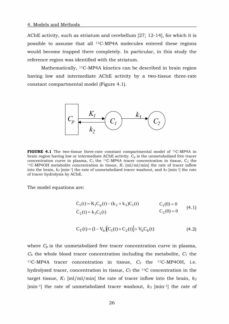
Mathematically, 11C-MP4A kinetics can be described in brain region
having low and intermediate AChE activity by a two-tissue three-rate
constant compartmental model (Figure 4.1).
K1
k2
k3Cp C1 C2
FIGURE 4.1 The two-tissue three-rate constant compartmental model of 11C-MP4A in brain region having low or intermediate AChE activity. Cp is the unmetabolized free tracer concentration curve in plasma, C1 the 11C-MP4A tracer concentration in tissue, C2 the 11C-MP4OH metabolite concentration in tissue, K1 [ml/ml/min] the rate of tracer inflow into the brain, k2 [min-1] the rate of unmetabolized tracer washout, and k3 [min-1] the rate of tracer hydrolysis by AChE.
The model equations are:
)t(Ck)t(C
)t(C)kk()t(CK)t(C
132
132p11
=
+−=
&
& (4.1)
0)0(C0)0(C
2
1
==
[ ] )t(CV)t(C)t(C)V1()t(C bb21bT ++−= (4.2)
where Cp is the unmetabolized free tracer concentration curve in plasma,
Cb the whole blood tracer concentration including the metabolite, C1 the 11C-MP4A tracer concentration in tissue, C2 the 11C-MP4OH, i.e.
hydrolyzed tracer, concentration in tissue, CT the 11C concentration in the
target tissue, K1 [ml/ml/min] the rate of tracer inflow into the brain, k2
[min-1] the rate of unmetabolized tracer washout, k3 [min-1] the rate of
26

4. Models and Methods
tracer hydrolysis by AChE, and Vb [unitless] is the fraction of the
measured volume occupied by blood. Because Vb in humans is around
5%, the blood term is often omitted. Thus, by assuming negligible blood
volume presence, i.e. Vb≅0, Eq. 4,2 becomes:
)t(C)t(C)t(C 21T += (4.3)
AChE activity was measured in terms of the rate constant for
hydrolysis of 11C-MP4A, k3.
In brain region having high AChE acitivty, it is normally assumed
that 11C-MP4A is so rapidly transformed into the hydrophilic metabolites
[11C]MP4OH that elimination of [11C]MP4OH from the brain can be ignored
[8] and, thus, 11C-MP4A kinetics can be described by a one-tissue one-rate
constant compartmental model [13] (Figure 4.2).
RK1Cp CR
FIGURE 4.2 The one-tissue one-rate constant compartmental model of 11C-MP4A in brain region having high AChE activity. Cp is the unmetabolized free tracer concentration curve in plasma, CR the 11C-MP4A tracer concentration in the target tissue, K1R [ml/ml/min] the joint rate constant of both tracer inflow into the tissue brain and tracer hydrolysis activity.
By assuming also in this region negligible blood volume presence, the
model equation is:
)t(CK)t(C pR1R =& (4.4) 0)0(CR =
where Cp is the unmetabolized free tracer concentration curve in plasma,
CR the 11C-MP4A tracer concentration in the target tissue, K1R
27

4. Models and Methods
[ml/ml/min] the joint rate constant of both tracer inflow into the tissue
brain and tracer hydrolysis activity.
The Reference Tissue Model for 11C-MP4A.
A reference model. i.e. a mathematical relationship for the region-of-
interest concentration in terms of the reference region data and the kinetic
parameters of both reference and target regions, can be derived by
combining Eqs. 4.1, 4.3, and 4.4. In fact, from Eq. 4.1, taking Laplace
transform:
)s(Ck)t(Cs
)s(CK)s(C)kks(
132
p1132
=⋅
=⋅++ (4.5)
and, from Eq. 4.4:
)s(CsK1)s(C RR1
p ⋅= (4.6)
Substituting Eq. 4.6 in Eq. 4.3, one obtains:
)s(C)kks(
kKK
)t(C
)s(C)kks(
sKK
)s(C
R32
3R1
12
R32
R1
11
⋅++
=
⋅++
=
(4.7)
and, from Eq. 4.3:
)s(C)kks(
ksKK)s(C)s(C)s(C R
32
3R1
121T ⋅
+++
=+= (4.8)
Finally, in temporal space, Eq. 4.8 returns:
ττ de)t(CkK)t(CK)t(C )t)(3k2k(t
0R2RRRT
−+−⋅⋅−⋅= ∫ (4.9)
where R1
1R
KK
K = [unitless]. Eq. 4.9 describes the reference model of 11C-
MP4A. The three-model parameter can be estimated together 32R k,k,K
28

4. Models and Methods
with their precision by using nonlinear weighted least squares (NLLS).
However, since NNLS is computational demanding when pixel-wise
quantification is performed, it is also possible to linearize the model of Eq.
4.9 and resort to less computational demanding algorithms. Up to now,
several different methods and linearized version of the model of Eq. 4.9
have been proposed for 11C-MPA4 quantification at pixel levels. Among all,
the three most promising have been used and compared together with an
additional novel method, developed during my Ph.D [33, 34] course: the
reference tissue linear least squares (RLS) proposed for 11C-MP4A by
Nagatsuka et al 2001 [12], the reference ratio exponential (RRE) approach
proposed by Herholz et al [13] and its version based on the use of a
different estimation approach (RRE_BF) [14]; the comparison technique is
the novel reference maximum a posteriori method (MAP). Results have
been also compared to those obtained by using the “standard” NNLS
estimator with model of Eq. 4.9.
4.1. RLS (Reference Tissue Based Linear Least Square Method) In the early eighties (1984), Blomqvist [46] developed an innovative linear
algorithm for the rapid calculation of the local rate constants for the
category of the irreversible tracers. Nagatsuka et al.[12], implemented
Blomqvist approach in case of 11C-MP4A.
By combining equation 4.1 and 4.3, one has:
( )∫∫ ∫∫ +−+=t
0T
t
0 032p31
t
0p1T d)(Ckkdd)(CkKd)(CK)t(C θθθττθθ
θ
(4.10)
Substituting Eq. 4.4 into Eq. 4.10:
∫∫ +−+=t
0 T32t
0 R3RRRT d)(C)kk(d)(CkK)t(CKC ττττ (4.11)
and assuming:
29

4. Models and Methods
)kk(pkKp
KKK
p
323
3R2
RR1
11
+−=⋅=
≡=
(4.12)
one has:
∫∫ ++=t
0 T3t
0 R2R1T d)(Cpd)(Cp)t(CpC ττττ (4.13)
Once obtained the estimates of , the original parameters
can be derived from:
321 p,p,p 32R k,k,K
1
232
1
23
1R
pp
pk
pp
k
pK
−−=
=
=
(4.14)
The three unknown parameters can be estimated by linear least
squares:
321 p,p,p
(4.15) yXXX T1T
3
2
1
)(ppp
−=⎥⎥⎥
⎦
⎤
⎢⎢⎢
⎣
⎡
where X is a N x 3 matrix, with N equal to the number of total frames, i.e.
measurements, built in this way:
⎥⎥⎥⎥⎥
⎦
⎤
⎢⎢⎢⎢⎢
⎣
⎡
=
∫ ∫
∫ ∫
Nt
0
Nt
0 TRNR
1t
0
1t
0 TR1R
d)(Cd)(C)t(C
d)(Cd)(C)t(C
ττττ
ττττ
MOMX (4.12)
TX is the transpose of X, and
⎥⎥⎥
⎦
⎤
⎢⎢⎢
⎣
⎡=
)t(C
)t(C
Ni
1i
My (4.13)
the vector of the measurements. Precision of parameter estimates can be
derived from the covariance matrix given by:
30

4. Models and Methods
(4.14) 1T
32313
23212
13121
)()p(VCovCov
Cov)p(VCovCovCov)p(V
−⋅=⎥⎥⎥
⎦
⎤
⎢⎢⎢
⎣
⎡XXφ
where mN
RSS−
=φ with m the number of unknown parameters (3 in this
case), and RSS representing the residual sum of squares evaluated at the
minimum, i.e.
[ ]∑=
−=N
1i
2i
ObsTiT )t(C)t(CRSS
(4.15)
with and the model predicted and measured PET activity.
The variances of estimates can be obtained by [12]:
)t(C iT )t(C iobsT
2R k,k,K 3
2332
1331
1221
3
2
32
2
21
2
132R
Covpp
2Covpp
2Covpp
2
)p(Vp
)p(Vp
)p(Vp
)k,k,K(V
⎟⎟⎠
⎞⎜⎜⎝
⎛∂∂
⎟⎟⎠
⎞⎜⎜⎝
⎛∂∂
+⎟⎟⎠
⎞⎜⎜⎝
⎛∂∂
⎟⎟⎠
⎞⎜⎜⎝
⎛∂∂
+⎟⎟⎠
⎞⎜⎜⎝
⎛∂∂
⎟⎟⎠
⎞⎜⎜⎝
⎛∂∂
+⋅⎟⎟⎠
⎞⎜⎜⎝
⎛∂∂
+⋅⎟⎟⎠
⎞⎜⎜⎝
⎛∂∂
+⋅⎟⎟⎠
⎞⎜⎜⎝
⎛∂∂
=
yyyyyy
yyy
(4.16)
Of note is that RLS method proposed in [12] does not use weights.
4.2. RRE (Reference Ratio Exponential Approach) A different approach for 11C-MP4A quantification have been developed by
Namba et al. [8]. The regional brain time-radioactivity curves CT(t) is again
described by using the two-tissue three-rate constant compartmental
model of Fig. 4.1, arterial input function and the Eq.4.1 and Eq. 4.3
solved to give:
∫∫ ++
+= −+− t
0 p32
31t
0)t)(kk(
p32
21T d)(C
kkkK
de)(Ckk
kK)t(C 32 ττττ τ (4.17)
Assuming that the reference region is described by the model of Eq. 4.4:
ττ d)(CK)t(Ct
0p
R1R ∫= (4.18)
31

4. Models and Methods
and considering the mathematical approach proposed by Herholz and his
colleagues [13]one can obtain C(t):
Bd)(C
de)(CA
)t(C)t(C)t(C t
0 p
t
0)t(K
p
R
T +==
∫∫ −−
ττ
ττ τ
(4.19)
where
][min kkK
]unitless[kk
kKKB
]unitless[kk
kKKA
132
32
3R1
1
32
2R1
1
−+=
+⋅=
+⋅=
(4.20)
By assuming, now, that there is a very rapid fall of non-hydrolyzed tracer
activity in plasma, the arterial input function, Cp(t), can be described by a
mono-exponential function:
tkp
pe)t(C −⋅=α (4.21)
with due to very rapid hydrolysis [13] of the tracer in plasma.
Thus, by substitution of Eq. 4.21 in Eq. 4.19:
Kk p >>
( )
( )
Be1
k1
1ekK
1eA
Bde
deeAB
de
deeA)t(C
tk
p
tkK
p
Kt
t
0k
t
0kKKt
t
0k
t
0)t(Kk
p
p
p
p
p
p
+
⎥⎦⎤
⎢⎣⎡ −
⎥⎦⎤
⎢⎣⎡ −
−=
+=+=
−
−−
−
−−
−
−−−
∫∫
∫∫
τ
τ
τα
τατ
τ
τ
ττ
(4.22)
Since , and, thus, Eq. 4.22 becomes: Kk p >>tkt)kK( pp ee −− ≈
BeA)t(C Kt +⋅= − (4.23)
The three model parameters, , can be estimated by nonlinear least
squares minimizing the weighted residuals sum of squares:
K,B,A
32

4. Models and Methods
[ ]∑=
−=
N
1i
2
2i
iObs
i )t(C)t(C)(WRSS
σp (4.24)
with vector of model parameters, N = number of total frames,
and the model predicted and measured ratio (i.e.
) PET activity. is the variance of the measurements errors
assumed to be uncorrelated and normally distributed with zero mean and
known with the exception of a term
T]K,B,A[=p
t(Cobs
)t(C/) R
)t(C i
t(CT
)i
2iσ
γ . The values are occasionally
referred to as weights. As C(t) expressed in Eq. 4.23 is obtained from the
ratio of two observed noise corrupted measures, the error propagation
must be consider during the parameters estimation process. Therefore,
variance δ2 was chosen to be equal to:
2i/1 σ
2i
i
iR
i
iT2i )t(t
)t(C)t(t)t(C σγγγδ ⋅=⎟⎟
⎠
⎞⎜⎜⎝
⎛Δ
+⎟⎟⎠
⎞⎜⎜⎝
⎛Δ
= (4.25)
where Δt(ti) is the scan interval at time ti. The scale factor γ is estimated a
posteriori [28] as:
mNpWRSS
−=
)ˆ(γ (4.26)
where is the value of the sum of squares of residuals evaluated
at the minimum.
)p̂(WRSS
The precision of estimates is obtained from the inverse of Fisher
information matrix F by approximate measures of the covariance matrix Σ
of estimation error : pp−ˆ
⎥⎥⎥
⎦
⎤
⎢⎢⎢
⎣
⎡== −
)B(VCovCovCov)k(VCovCovCov)A(V
3231
2321
13121FΣ (4.27)
where F is the Fisher information matrix:
SRSF 1Tp̂p|)p( −
= = (4.28)
with S the sensitivity matrix of the model of Eq. 4.23, given by:
33

4. Models and Methods
⎥⎥⎥⎥⎥⎥
⎦
⎤
⎢⎢⎢⎢⎢⎢
⎣
⎡
∂∂
∂∂
∂∂
∂∂
∂∂
∂∂
∂∂
∂∂
∂∂
=
K)t,p(C......
K)t,p(C
K)t,p(C
B)t,p(C......
B)t,p(C
B)t,p(C
A)t,p(C......
A)t,p(C
A)t,p(C
)i,k(
N21
N21
N21
S (4.29)
and R the known N x N weighted matrix:
N,..,1i),/1(diagR 2i == δ (4.30)
Then the percent coefficient of variation of the estimates =[A, K, B], p̂
)p̂(CV k , is given by:
)3m(m,...,1k,100p̂
)k,k()p̂(CV
kk ==×
Σ= (4.31)
Finally, and values obtained from: 2k 3k
][minKBA
Ak
][minKBA
Bk
12
13
−
−
⋅+
=
⋅+
= (4.32)
The variance of k3, i.e. the most interesting parameter, can be derived by
using linear error transfer function as follows:
2333
1333
1233
23
23
23
3
CovKk
Bk2Cov
Bk
Ak2Cov
Kk
Ak2
)B(VBk)K(V
Kk)A(V
Ak)k(V
⋅⎟⎠⎞
⎜⎝⎛
∂∂⋅
∂∂
+⋅⎟⎠⎞
⎜⎝⎛
∂∂⋅
∂∂
+⋅⎟⎠⎞
⎜⎝⎛
∂∂⋅
∂∂
+
⋅⎟⎠⎞
⎜⎝⎛∂∂
+⋅⎟⎠⎞
⎜⎝⎛∂∂
+⋅⎟⎠⎞
⎜⎝⎛∂∂
= (4.33)
4.3. RRE_BF model (Reference Ratio Exponential based on Basis Function Approach) Recently, Zundorf and his colleagues [14] extended and modified the non-
invasive technique proposed by Herholz [13] based on reference ratio
exponential (RRE) for the quantitation of AChE activity by 11C-MP4A PET.
They extend and modify this method in order to generate parametric
images for analysis of local AChE activity without need for definition of
34

4. Models and Methods
region of interest and to further improve the numerical representation of
the input function by eliminating off the unnecessary mono-exponential
approximation.
The method in based on the compartmental kinetic model of the
tracer described in Eq. 4.19 (Figure 4.1) where Eq.4.18 is used to
substitute Cp:
B)t(C
de)(CK)t(CA
B)t(C
de)(CKe)t(Ce
A
B)t(C
de)(CeAB
)t(C
de)(CA
)t(C)t(C)t(C
R
t
0
)t(KRR
R
t
0
KR
KtR
Kt
R
t
0K
RKt
R
t
0)t(K
R
R
T
+
−
=
+⎪⎭
⎪⎬⎫
⎪⎩
⎪⎨⎧
−
=
+=+==
∫
∫
∫∫
−
−
−−−
ττ
ττ
ττττ
τ
τ
ττ &&
(4.34)
And, finally, one has:
BtWABtC
deCKAtC K
R
ttK
R
+⋅=+
⎥⎥⎥⎥⎥
⎦
⎤
⎢⎢⎢⎢⎢
⎣
⎡
−=∫ −
)()(
)(1)( 0
)( ττ τ
(4.35)
As seen for REE method, the three model parameters, , can
be estimated by nonlinear least squares, which is a time consuming
approach above all if pixel-by-pixel quantification is required. In order to
speed up the quantification process, a basis function approach [14] can be
used. Following this approach,
K,B,A
)t(WK is calculated by numeric integration
for a set of different K that covers the entire range of interest.
Subsequently, for each K values, A and B are estimated by weighted linear
least square estimator. In particular, having K fixed to a specific value:
35

4. Models and Methods
yRXRXX ⋅⋅=⎥⎦
⎤⎢⎣
⎡ − T1T )(BA
(4.36)
where X is a N x 2 matrix, with N equal to the number of total frames, i.e.
measurements, built in this way:
⎥⎥⎥
⎦
⎤
⎢⎢⎢
⎣
⎡=
)t(W1
)t(W1
NK
1K
MMX (4.37)
TX is the transpose of X, and
⎥⎥⎥
⎦
⎤
⎢⎢⎢
⎣
⎡=
⎥⎥⎥
⎦
⎤
⎢⎢⎢
⎣
⎡=
)t(C/)t(C
)t(C/)t(C
)t(C
)t(C
NRNT
1R1T
N
1
MMy (4.38)
the vector of the measurements. R is the known N x N weighted matrix:
N,..,1i),/1(diagR 2i == σ (4.39)
with as in 4.24. The covariance matrix for A and B is given by: 2iσ
(4.40) 1T
212
121 )RXX()p(VCov
Cov)p(V −=⎥⎦
⎤⎢⎣
⎡γ
with γ as in Eq.4.26.
Final optimum estimates of A, B, and K will coincide with the
parameters set for which the weighted sum of residuals is smallest.
Finally, k3 and k2 estimates are obtained from equations 4.32 and an
underestimation of the variance of k3 from:
1233
23
23
3 CovBk
Ak2)B(V
Bk)A(V
Ak)k(V ⋅⎟
⎠⎞
⎜⎝⎛
∂∂⋅
∂∂
+⋅⎟⎠⎞
⎜⎝⎛∂∂
+⋅⎟⎠⎞
⎜⎝⎛∂∂
= (4.41)
In order to estimate a physiological grid for parameter K variation,
i.e. the K minimum and maximum values, no information is giving about
the range choose and about the number of values considered for the range
interval, the so called basis function. Therefore, based on the information
already published on k2 and k3 estimates we calculate Kmin and a Kmax as:
36

4. Models and Methods
max3max2max
min3min2min
kkK
kkK
+=
+= (4.42)
We choose the range interval for K such that:
max'maxmin
'min KKandKK >< (4.43)
Three different assumptions for K have been made:
1. K range between 0.05 and 0.5 with NBF=100 (C1);
2. K range between 0.01 to 1 with NBF=100 (C2);
3. K range between 0.01 to 1 with NBF=200 (C3);
where NBF denotes the basis function number.
4.4. R-NLLS (Reference Tissue based Non Linear
Least Square Method) The standard method to estimate regional hydrolysis rate of AChE using 11C-MP4A images is to fit the regional time-activity curve (TAC) obtained
by PET to the theoretical function derived from the kinetic model and the
arterial input function using weighed nonlinear least squares (NLS)
optimisation. In this study we also evaluated the results obtained by using
model of Eq. 4.9 and the weighted nonlinear least squares estimator.
Thus, the three rate constants, i.e. KR, k2, k3 , are estimated by minimizing
the following objective function:
∑=
−=
N
1i
2
2i
iTiobsT )]t,p(C)t(C[)p(WRSS
σ (4.44)
with vector of model parameters, N = number of total
frames, and the model predicted and measured PET
activity. is known as the variance of the measurements errors
assumed to be uncorrelated and normally distributed with zero mean. The
total error variance δ2 was chosen to be equal to:
T32R ]k,k,K[=p
)t(C iT
2iσ
)t(C iobsT
37

4. Models and Methods
2i
i
iT2i )t(t
)t(C σγγδ ⋅=⎟⎟⎠
⎞⎜⎜⎝
⎛Δ
= (4.45)
where Δt(ti) is the scan interval at time ti. The scale factor γ is estimated a
posteriori [28] as in Eq. 4.26. The precision of estimates is obtained from
Eq. 4.27 , i.e. from the inverse of Fisher information matrix and the
percent coefficient of variation of the estimates obtained from Eq. 4.31.
4.5. MAP (Reference Tissue based Maximum a Posteriori Parameter Estimation) The maximum a posteriori (MAP) estimator is closely related to the
Fisherian method of maximum likelihood (ML). The ML estimator
maximize the likelihood function, which is the conditional probability of
data given the parameter vector [30, 31]. The MAP estimator expands this
concept and considers not only the likelihood function but also the known
a priori probability of the parameters [47]. MAP estimation is a Bayesian
approach since a priori available statistical information on the unknown
parameters is also exploited for their estimation. The updated probability,
the so called a posteriori probability, is obtained according to the Bayes’
theorem:
)(f)(f)|(f)|(f obs
T
obsTobs
TC
ppCCp = (4.46)
where f(p) is the prior probability of model parameters p, is the
prior probability of measurements , and is the conditional
probability of measurements given the parameter vector p. The
denominator in Eq. 4.46 is called the normalization factor and is
independent of the paramaters.. Thus, ignoring the denominator in Eq.
4.46, which is independent on p, Eq. 4.46 can be rewritten as:
)(f obsTC
obsTC )|(f obs
T pC
obsTC
)(f)|(f)|(f obsT
obsT ppCCp ∝ (4.47)
38

4. Models and Methods
Finally, parameter estimates can be obtained by using a MAP estimator
maximizing:
(4.48) )](f)|C(f[maxargˆ obsTMAP ppp
p=
A preliminary reference weighted non linear least squares (R-NLLS)
analysis at TAC_ROI level was implemented in SAAM II software that is a
general purpose modelling tool with a user friendly interface based on
compartmental models; SAAM II software allows a fast kinetic analysis -
for TAC_ROIs - in order to identify the parameters of interest(KR, k2, k3). k2
showed a low inter-region variability within subject (as already confirmed
in the literature by Namba[8] and Herholz [10, 13] in a range of 0.08-
0.12); it was assumed that k2 has a priori Gaussian probability density
function with mean and standard deviation equal to k2 mean and SD
estimates obtained with R-NLLS at TAC_ROI level for each subject. This
additional probabilistic information was used to estimate tracer kinetic
indexes at pixel and TAC_ROI level in MAP approach. In particular,
assuming that k2 model parameter and its measurement error have a
Gaussian distribution, Eq. 4.48 can be shown to become:
)k()k(
]CC[R]CC[minargˆ
2k212k
T2k2
TobsT
1TT
obsT
pMAP
μμ −Ω−+
−−=
−
−p (4.49)
where p is the parameter vector p=[KR, k2, k3]T, is the measurement
vector, is the vector prediction of the model of Eq. 4.9,
obsTC
TC 2kμ is the a
priori mean vector and the respective inverse of the covariance matrix.
R-1 represents the inverse of the measurement error variance: the
measurements has been chosen Gaussian, with zero mean and variance
equal to δ2=
12k
−Ω
γ CT(ti)/Δt(ti) where Δt(ti) is the scan interval at time ti. The
scale factor γ is estimated a posteriori [28] as:
mNpWRSS
−=
)(^
γ (4.50)
39

4. Models and Methods
where is the value of the cost function evaluated at the minimum,
i.e., for p equal to the vector of estimated model parameters .
)(^pWRSS
^p
The precision of MAP estimates can be obtained from the covariance
matrix of the estimation error [30]: 11
2kT1
MAP )SSR( −−− Ω+=Σ (4.51)
where S is the sensitivity matrix of the model equation 4.9, the matrix
with entries given by:
p̂pittk
ip
)t,p(C)i,k(S
==
∂∂
=for N,...,1i;m,..,1k == (4.52)
Then the percent coefficient of variation of the estimates (KR, k2, k3),
is calculates using the same approach as in R-NLLS technique by:
kp^
)(^
kpCV
)3(,...,1,100),(
)( ^
^==×
Σ= mmk
p
kkpCV
k
MAPk and (4.63) RKp =1
^
The name MAP just reflects the fact that point estimates are those
which maximize the a posteriori probability density function, or equally
minimize the cost function, given the a priori probability density function,
the model structure, and the measurement error statistical description.
4.6. Parametric Images Processing In order to obtain functional parametric images of KR, k2 and k3, the
mathematical methods previously described were implemented in Matlab
software and applied to the 4D PET dynamic images (the originally
reconstructed 4D PET images with voxels size of 2.5x2.5x4.25 mm).
The functional parametric images are processed as follows:
1. All parametric images (KR, k2, k3) are "cleaned" in order to have only
reliable estimates.
2. Images from step 1 are then smoothed using a median filter.
40

4. Models and Methods
3. Smoothed parametric images undergoes step 3 to step 7 presented
in chapter 3 for dynamic image processing: normalization to PET-
FDG template (SPM2), coregistration to the single-subject canonical
template(SPM2), extraction of quantitative information applying the
masks ROIs generated with Marina software.
The flowchart of functional parametric images generation and
processing is shown in figure 4.3. Two tailed unpaired t-test was applied
to quantify the differences in k3 estimates at pixel level obtained by each
procedure between the two groups of subjects. The value of p for which
the differences were considered significant is p<0.05.
Functional Parametric Image Processing
FIGURE 4.3 The flowchart of 4D 11C-MP4A PET images processing at pixel-by-pixel level
41

4. Models and Methods
42

5. Results
Chapter 5
Results
AChE activity was measured in terms of the rate constant for hydrolysis of 11C-MP4A, k3. In particular, the methods described in the previous
chapter are used in order to determine the quantitative kinetics indexes
without arterial blood sampling and are as follows: the method proposed
in the literature: reference tissue linear least squares (RLS) proposed by
Blomqvist [46] and validated by Nagatsuka et al 2001 [12], reference ratio
exponential (RRE) approach proposed by Herholz and coworkers in 2001
[13], Zundorf et al that used a modified simplification hypothesis of
Herholz approach in order to reduce unnecessary bias and implemented a
basis function approach in order to estimate the parameters of interest
[14]; the new proposed approaches based on reference tissue nonlinear
least squares (R-NLLS) and reference maximum a posteriori method
(MAP).
5.1. RLS results and discussion RLS approach was applied at both pixel (pTAC) and ROI (TAC_ROI) level in
order to obtain k3 estimates. Precision of estimates was measured in terms
of variation coefficient (CV) described in section 4.1. Parametric images of
KR, k2 and k3 of the entire dataset were filtered for the pixels estimated
with precision higher than 300 and k3 values higher than 0.95 min-1.
Thus were obtained only reliable parametric images of the indexes
43

5. Results
describing tracer kinetics that undergoes parametric images processing
flowchart presented in section 4, figure 4.3.
AChE activity is measured in terms of tracer hydrolysis rate
constant k3. Average k3 parametric images for both groups of subjects are
shown in figure 5.1: in panel A are represented the lower slices of the
brain containing anatomical structure like cerebellum, hippocampus (HP),
temporal (TE) and frontal (FR) lobe, while in panel B are represented brain
structure like thalamus (TH), basal ganglia (GB), TE, FR, occipital (OC),
insula (I) and initial of parietal (PA) lobe. Each panel represents the mean
k3 parametric image of the NC in the top line and AD in the bottom line.
All images are represented using the same image scale: [0, 0.4] min-1.
Two tailed t-test was applied in order to identify differences in k3
estimates between the two groups of subjects.
Despite the small group of dataset – 4NC and 7AD – RLS method
applied at pixel level identify significant reduction of AChE activity in AD
patients respect to normals in area with low enzyme expression like FR,
TE, PA, OC (Table 5.1) with p<0.005. However, no differences were
identified applying the same mathematical approach at TAC_ROI level
except the Rolandic operculum region (R).
TABLE 5.1 RLS k3 indexes obtained at pixel-by-pixel level and TAC_ROI level in brain area with low enzyme activity (neocortex) and low to moderate (HP, R, I) and moderate (TH) enzyme expression in both group of subjects and the respective p value.
44

5. Results
RLS method is not able to give reliable estimates of k3 indexes when
applied at pixel level in area with moderate enzyme activity like thalamus
and low to moderate as hippocampus (see Table 5.1 and FIGURE. 5.2)
even if identifies a significant difference in k3 values between the groups of
subjects (p=0.007 for TH) (Table 5.1).
k3 estimates obtained at TAC_ROI level show a mean variation of
+11% in NC and +22% in AD respect to k3 estimates at pixel level for the
neocortex area and a higher variation of estimates in TH and HP regions:
+67% in NC and +72% AD for TH and +37% in NC and +59% in AD
respect to k3 index estimated in the same areas at pixel level. (FIGURE
5.2). The variation between the pixel and TAC_ROI estimates was
calculated as (1-pixel_k3/TAC_ROI_k3)*100.
Namba and his colleagues [8] identify k3 estimates in neocortex area
in 20 normals subjects using the standard quantification model at
TAC_ROI level and arterial input function. The mean value identified on
neocortex – as mean of k3 estimates in FR, OC, TE, PA lobes – was 0.076 ±
0.008 that was considered the “true” k3 value in NC. Bias of mean k3
values estimated in neocortex area at pixel and TAC_ROI level was
calculated respect to the considered “true” value as follows:
1001_
_%
3
3 ∗⎟⎟⎠
⎞⎜⎜⎝
⎛−=
ktruekestimated
bias (5.1)
The results obtained applying RLS mathematical approach at pixel
level underestimates about 7% the “true” k3 while there is an
overestimation of 4% of k3 index in case of TAC_ROI approach in cortex
area with low enzyme expression. Considering the high variation between
pixel and TAC_ROI of k3 estimates in neocortex area in AD subjects (22%,
Table 5.1), RLS might be a good model to be applied at pixel-by-pixel level
in order to preserve all the information of tracer kinetics in case of
neurodegeneration and to estimate k3 in area with low enzyme activity.
45

5. Results
Panel A
NC
0
0.4
[min-1]
0
0.4
[min-1]
0
0.4
[min-1]
AD
Panel B
NC
0
0.4
[min-1]
0
0.4
[min-1]
0
0.4
[min-1]AD
FIGURE 5.1 Average of normalized and co-registered parametric image of k3 obtained with RLS mathematical procedure for both groups of subjects: NC upper line and AD bottom line in Panel A and Panel B. Image scale: [0, 0.4] min-1.
46

5. Results
RLSPixel-by-pixel k3 estimates
FR OC PA TE I HP R TH
k 3 [
min
-1 ]
0.00
0.05
0.10
0.15
0.20
0.25
0.30
NCAD
RLS TAC_ROI k3 estimates
FR OC PA TE I HP R TH
k 3 [m
in-1
]
0.00
0.05
0.10
0.15
0.20
0.25
0.30NCAD
RLSPixel-by-pixel vs TAC_ROI k3estim ates
FR OC PA TE I HP R TH
k 3 [min
-1]
0 .00
0.05
0.10
0.15
0.20
0.25
0.30
NC pxpNC TAC_ROIAD pxpAD TAC_ROI
FIGURE 5.2 RLS k3 estimates at pixel-by-pixel (pxp) level (top panel), TAC_ROI level (middle panel) and comparison pixel vs TAC_ROI estimates (bottom panel).
47

5. Results
5.2. RRE results and discussion Parametric images of k3 obtained with the ratio approach [13] undergoes
the steps for image processing described in the flowchart from Figure 4.3
in order to have reliable filtered, normalized and corregistered images
(Figure 5.3).
Two tailed t-test was applied in order to identify differences in k3
estimates between the two groups of subjects.
RRE method applied at pixel level identify significant reduction of AChE
activity in AD patients respect to normals only in FR lobe from the
neocortex area, p<0.05. In the TH, I, and R area were also identify
significant differences between the studied groups (table 5.2). However, no
significances were identified applying the same mathematical approach at
TAC_ROI level in the neocortex area as shown in table 5.2.
TABLE 5.2 RRE k3 indexes obtained at pixel-by-pixel level and TAC_ROI level in brain area with low enzyme activity (neocortex) and low to moderate (HP, R, I) and moderate (TH) enzyme expression in both group of subjects and the respective p value.
The brain areas where the model seemed to be conservative in
identifying significant differences between normals and AD patients, no
matter if applied at pixel or TAC_ROI level are represented by insula and
Rolandic operculum (R).
k3 estimates obtained at TAC_ROI level show a mean variation of -
7% in NC and AD respect to k3 estimates at pixel level for the neocortex
area and a higher variation of estimates in TH and HP regions: +10% in
NC and +22% AD for TH and -8% in NC and +4% in AD respect to k3 index
48
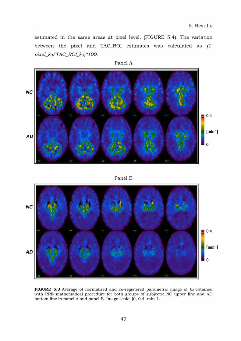
5. Results
estimated in the same areas at pixel level. (FIGURE 5.4). The variation
between the pixel and TAC_ROI estimates was calculated as (1-
pixel_k3/TAC_ROI_k3)*100.
Panel A
NC
0
0.4
[min-1]
0
0.4
[min-1]
0
0.4
[min-1]AD
Panel B
NC
0
0.4
[min-1]
0
0.4
[min-1]
0
0.4
[min-1]AD
FIGURE 5.3 Average of normalized and co-registered parametric image of k3 obtained with RRE mathematical procedure for both groups of subjects: NC upper line and AD bottom line in panel A and panel B. Image scale: [0, 0.4] min-1.
49

5. Results
RREpixel-by-pixel k3 estimates
FR OC PA TE I HP R TH
k 3 [m
in-1
]
0.00
0.05
0.10
0.15
0.20
0.25
0.30NC AD
RRETAC_RO I k3 estim ates
FR O C PA TE I HP R TH
k 3 [m
in-1
]
0 .00
0.05
0.10
0.15
0.20
0.25
0.30NC AD
R R Ep ix e l-b y -p ix e l v s T A C _ R O I k 3 e s t im a te s
F R O C P A T E I H P R T H
k 3 [min
-1 ]
0 .0 0
0 .0 5
0 .1 0
0 .1 5
0 .2 0
0 .2 5
0 .3 0N C p x pN C T A C _ R O IA D p x pA D T A C _ R O I
FIGURE 5.4 RRE k3 estimates at pixel-by-pixel (pxp) level (top panel), TAC_ROI level (middle panel) and comparison pixel vs TAC_ROI estimates (bottom panel).
50

5. Results
However, the results obtained applying the model at pixel level
presented in Table 5.2 are not in good agreement with the published data
in the literature [13, 19].
Therefore we verify the performance of RRE in estimating k2 and it
was observed inaccurate estimates of this parameter. In order to consider
only reliable parameter estimates, RRE parametric images have been
filtered by calculate a threshold for k2 estimates. The threshold was
estimated in each subject from the k2 parametric image as the mean k2
value to which wad added twice the standard deviation. A uniform k2
threshold of 2 min-1 was obtained for each person participated in the
study. In this way, only pixels having reliable estimates for RRE model
parameters are taken into account. The new k3 estimates obtained by RRE
corrected for the threshold (RRE_t) are reported in table 5.3.
TABLE 5.3 RRE k3 indexes obtained at pixel-by-pixel level before (RRE) and after threshold correction (RRE_t) in brain area with low enzyme activity (neocortex) and low to moderate (HP, R, I) and moderate (TH) enzyme expression in both group of subjects and the respective p value.
The mean k3 estimates at pixel level corrected for the threshold
(RRE_t), in neocortex area are 10% lower in NC and 45% decreased in AD.
The TH and HP corrected k3 indexes showed a higher decrease of 47% in
NC and 74% in AD for TH and 30% in normals and 67% in pathologic
subjects for HP region respect to non corrected k3 indexes for the same
brain areas. Corrected parametric images of k3 in both group of subjects
showed significant differences respect to non corrected parametric images
of the same study groups (FIGURE 5.5). Anyway, the k3 estimates
51

5. Results
corrected for the threshold are to be considering reliable for further
comparison.
FIGURE 5.5 Average of normalized and co-registered parametric image of k3 obtained with RRE mathematical procedure not corrected (RRE) and corrected with the threshold (RRE_t) for both groups of subjects: NC (RRE_NC, RRE_t_NC) left part of the panel and AD (RRE_AD, RRE_t_AD) located on the right part of the panel. Images scale: [0, 0.4] min-
1.
Bias of mean k3 values estimated in neocortex area at pixel (RRE_t)
and TAC_ROI level was calculated respect to the considered “true” value
identified by Namba [8] as follows:
1001_
_%
3
3 ∗⎟⎟⎠
⎞⎜⎜⎝
⎛−=
ktruekestimated
bias (5.1)
The results obtained applying RRE mathematical approach with the
correction for the threshold at pixel level underestimates about 14% the
“true” k3 while there is an underestimation of 12% of k3 index in case of
TAC_ROI approach in neocortex area.
We also consider the “true” values of k3 index in TH (0.266 min-1)
and HP (0.11 min-1) region as the ones identified by Nagatsuka and his
52

5. Results
colleagues [12] in normal subjects, using the standard non linear
estimation method with arterial input.
The bias calculated with equation 5.1 revealed an underestimation
of pixel-by-pixel k3 indexes in NC of 55% for TH and 25% for HP. In case of
TAC_ROI k3 estimates the identified bias for both TH and HP revealed an
underestimation of 26% respect to the considered “true” k3 values.
RRE_t is not a reliable method for the estimation of k3 index in area
with low to moderate and moderate AChE activity, and proved to have
difficulties in giving reliable estimates even in brain area with low enzyme
expression.
5.3. RRE_BF results and discussion. Recently, Zundorf and his colleagues [14] extended and modified the non-
invasive technique proposed by Herholz [13] based on reference ratio
exponential (RRE) for the quantitation of AChE activity by MP4A PET.
We applied this new proposed technique at pixel-by-pixel level,
without applying the smooth of 10 mm FWHM Gaussian filter to the PET
dynamic image as described [14]. We also considered in the analysis – as
shown in flowchart presented in figure 4.2 - all brain pixels in order to
calculate k3 and k2 (Eq. 4.32) by estimation of A, B, and K from the
weighted linear procedure previously described (See chapter 4, subsection
4.3). As in the RRE approach, k3 parametric images are filtered for the
value k2 threshold of 2 in order to consider only reliable estimates.
Striatum was used as reference region.
Three different assumptions for K have been made:
4. K range between 0.05 and 0.5 with NBF=100 (C1).
5. K range between 0.01 to 1 with NBF=100 (C2).
6. K range between 0.01 to 1 with NBF=200 (C3).
Groups mean has been compared by applying two tailed sample t-
test on the mean cortical k3 values of the subjects. The mean k3 values
were calculated by averaging all voxels of the parametric image within the
53

5. Results
standard ROI masks generated with Marina software as already described
(flowchart in figure 4.3).
Mean, normalized and co-registered k3 parametric image for both
groups of subjects (NC and AD), obtained applying RRE_BF technique
considering the three different conditions (C1, C2, C3) are shown in
FIGURE 5.6.
RRE_BF method applied at pixel level identify significant reduction
of AChE activity in AD patients respect to normals only in PA lobe from
the neocortex area, in the TH, I, and R area, with p<0.05, when assuming
condition C1 for K index; in TH, I, R in case of C2 condition and at I and R
area level for C3 (see TABLE 5.4).
No improvement in model performance is observed when consider
the other two assumption, for K, C2 and C3, in order to calculate k3 index
at neocortex level. A slight improvement in the performance of the
procedure is identifying in case of C2 condition for TH (Table 5.4, Figure
5.7).
The variation of k3 estimates when considering the three conditions
for K are calculated as follows:
(1-C1_estimate/C2_estimate)*100 for NC and respectively AD.
(1-C2_estimate/C3_estimate)*100 for NC and respectively AD.
The variation analysis on k3 estimates obtained with basis function
approaches revealed that when K range is increased (from C1 to C2 with
constant NBF) at neocortex level we have a decreased in estimates of 2%
in NC and 5% in AD subjects, in TH this variation is higher: +14% in NC
and +5% in AD while at HP level we have a variation of +5% in both
groups.
In case of the same K interval but a doubled increased NBF (C2 to
C3) the variation of k3 estimates at neocortex level is around 3% in NC and
less than 1% in AD. A higher variation was identified in case of TH: a
decreased in k3 estimates of 13% for NC and a little variation of less than
1% in AD.
54

5. Results
TAB
LE 5.4 R
RE
_BF m
ean k
3 indexes obtain
ed at el-by-pixel level (con
sidering th
e three assu
mption
s of range(b) and
nu
mber of basis fu
nction
(NB
F)) in brain area
zyme activity (n
eocortex) and low
toerate (H
P, R, I) and
moderate (TH
) enzym
e expression in
both grou
p of jects an
d the respective p valu
e.
pixw
ith low
ensu
b
mod
55

5. Results
Mean k3 values estimated in neocortex area at pixel level for normal
subjects were also compare to the considered “true” value identified by
Namba [8] for NC .
A bias was calculated as follows:
1001_
_%
3
3 ∗⎟⎟⎠
⎞⎜⎜⎝
⎛−=
ktruekestimated
bias (5.1)
The results obtained applying RRE_BF mathematical approach at
pixel level while considering the three different assumption (C1, C2 and
C3) give good mean estimates in C1 condition (bias 0.3%), underestimates
about 2% the “true” k3 when considering C2 and there is an
underestimation of 5% of k3 index in case of C3 approach in neocortex
area.
We also consider the “true” values of k3 index in TH (0.266 min-1)
and HP (0.11 min-1) region as the ones identified by Nagatsuka and his
colleagues [12] in normal subjects, using the standard non linear
estimation method with arterial input.
The bias calculated with equation 5.1 revealed an underestimation
of pixel-by-pixel mean k3 indexes in NC for TH of 43% , 34% and 41%
when consider assumption C1, C2 and respectively C3. A lower variation
in mean k3 estimates was revealed for HP respect to the considered “true”
k3 values: -0.4% for C1, +7% case C2 and 3% for assumption C3.
Basis function approach [14] of Herholz method [13] was developed
in order to obtain k3 index in area with low enzyme activity. The results
obtained applying RRE_BF technique to our data set is not in good
agreement with the already published results [14]: in our case the method
does not indicate a high sensitivity in detecting mild reduction of AChE
activity early in the course of AD. However, since k3 estimates in neocortex
area calculated in case of C1 assumption for K showed the smallest bias
respect to the considered true k3 value, these indexes are going to be used
in further models performance comparison.
56

5. Results
Panel A
0
0.4
[min-1]
0
0.4
[min-1]
0
0.4
[min-1]
Panel B
0
0.4
[min-1]
0
0.4
[min-1]
0
0.4
[min-1]
Panel C
0
0.4
[min-1]
0
0.4
[min-1]
0
0.4
[min-1]
FIGURE 5.6 Average of normalized and co-registered parametric image of k3 obtained with RRE_BF mathematical procedure for both groups of subjects: NC upper line and AD bottom line in each panel considering the assumption on K index: C1 in panel A, C2 in panel B and C3 in panel C. Images scale: [0, 0.4] min-1.
57

5. Results
Panel A
Panel B
FIGURE 5.7 RRE_BF k3 estimates at pixel-by-pixel level in NC vs AD when consider the different assumption for K (panel A) and the variation of the mean estimates within subject group (NC and respectively AD group) in Panel B.
58

5. Results
5.4. R-NLLS results and discussion. The R-NLLS algorithm was applied at both pixel and ROI level. Parametric
images were filtered and then transformed in order to the scheme
presented in figure 4.3 presented in section 4 of this work in order to have
reliable estimates.
Mean image of k3 estimates obtained with the reference tissue based non
linear technique are shown in FIGURE 5.8 for both groups of subjects.
Two tailed t-test was applied in order to identify differences in k3
estimates between the two groups of subjects.
R-NLLS method applied at pixel level identify significant reduction of
AChE activity in AD patients respect to normals in all the neocortex area,
p<0.05. In the TH, I, and R area were also identify significant differences
between the studied groups (Table 5.5). However, no significances were
identified applying the same mathematical approach at TAC_ROI level in
the neocortex area neither in TH or HP as shown in table 5.5.
k3 estimates obtained at TAC_ROI level show a mean variation of
+11% in NC and +20% in AD respect to k3 estimates at pixel level for the
neocortex area and a higher variation of estimates in TH and HP regions:
+54% in NC and +76% in AD for TH and +29% in NC and +48% in AD
respect to k3 index estimated in the same areas at pixel level (FIGURE
5.9). The variation between the pixel and TAC_ROI estimates was
calculated as (1-pixel_k3/TAC_ROI_k3)*100.
TABLE 5.5 R-NLLS k3 indexes obtained at pixel-by-pixel level in brain area with low enzyme activity (neocortex) and low to moderate (HP, R, I) and moderate (TH) enzyme expression in both group of subjects and the respective p value.
59

5. Results
Panel A
NC
0
0.4
[min-1]
0
0.4
[min-1]
0
0.4
[min-1]AD
Panel B
NC
0
0.4
[min-1]
0
0.4
[min-1]
0
0.4
[min-1]AD
FIGURE 5.8 Average of normalized and co-registered parametric image of k3 obtained with R-NLLS mathematical procedure for both groups of subjects: NC upper line and AD bottom line in panel A and panel B. Image scale: [0, 0.4] min-1.
60

5. Results
R_NLLS pixel-by-pixel k3 estimates
FR OC PA TE I HP R TH
k 3 [m
in-1
]
0.00
0.05
0.10
0.15
0.20
0.25
0.30NCAD
R_NLLS TAC_ROI k3 estimates
FR OC PA TE I HP R TH
k 3 [m
in-1
]
0.00
0.05
0.10
0.15
0.20
0.25
0.30NC AD
R _N L L SP ixe l-b y-p ixe l vs T A C _R O I k 3 es tim ates
F R O C P A T E I H P R T H
k 3 [m
in-1
]
0 .00
0 .05
0 .10
0 .15
0 .20
0 .25
0 .30N C pxpN C T A C _R O IA D pxpA D T A C _R O I
FIGURE 5.9 R-NLLS k3 estimates at pixel-by-pixel level (top panel), TAC_ROI level (middle panel) and comparison pixel vs TAC_ROI estimates (bottom panel).
61

5. Results
Bias of mean k3 values estimated in neocortex area at pixel and
TAC_ROI level was calculated respect to the considered “true” value
identified by Namba [8]. We also consider the “true” values of k3 index in
TH (0.266 min-1) and HP (0.11 min-1) region as the ones identified by
Nagatsuka and his colleagues [12] in normal subjects, using the standard
non linear estimation method with arterial input.
The bias values was calculated as presented in equation 5.1:
1001_
_%
3
3 ∗⎟⎟⎠
⎞⎜⎜⎝
⎛−=
ktruekestimated
bias (5.1)
The results obtained applying R-NLLS technique at pixel level
underestimates about 10% the “true” k3 while a low underestimation of
1% was revealed for k3 index in case of TAC_ROI approach in neocortex
area.
The bias calculated with equation 5.1 showed an underestimation of
pixel-by-pixel k3 indexes in NC of 68% for TH and 24% for HP. In case of
TAC_ROI k3 estimates the identified bias for TH was -30% while for HP
revealed a variability of +6% respect to the considered “true” k3 values.
R-NLLS procedure revealed also a variation between k3 estimates at
pixel-by-pixel level respect to TAC_ROI level. However, k2 indexes show a
very low inter-variability within subject at both level analysis. Therefore k2
will be used as a priori information in the new proposed mathematical
approach in order to improve the precision of k3 estimates.
5.5. MAP results and discussion. Bayesian algorithm (MAP) was applied at both pixel and ROI level.
Parametric images were filtered and then transformed as described in
section 4 of this work (FIGURE 4.3) in order to be considered only reliable
estimates of all indexes.
Mean image of k3 estimates obtained with the reference tissue based
MAP approach are shown in Figure 5.10 for both groups of subjects.
62

5. Results
Two tailed t-test was applied in order to identify differences in k3
estimates between the two groups of subjects.
Despite the small group of dataset – 4NC and 7AD – MAP method
applied at pixel level identify significant reduction of AChE activity in AD
patients respect to normals in area with low enzyme expression like FR,
TE, PA, OC (Table 5.6) and also in area with moderate enzyme expression
as TH and HP, with a p<0.05. However, no differences were identified
applying the same mathematical approach at TAC_ROI level except the
Rolandic operculum region (R) as it revealed in table 5.6.
k3 estimates obtained at TAC_ROI level show a mean variation
of -10% in NC and +0.4% in AD respect to k3 estimates at pixel level for
the neocortex area and a higher variation of estimates in TH and HP
regions: -4% in NC and +25% in AD for TH and -15% in NC and +14% in
AD respect to k3 index estimated in the same areas at pixel level (FIGURE
5.11). The variation between the pixel and TAC_ROI estimates was
calculated as (1-pixel_k3/TAC_ROI_k3)*100.
TABLE 5.6 MAP k3 indexes obtained at pixel-by-pixel and TAC_ROI level in brain area with low enzyme activity (neocortex) and low to moderate (HP, R, I) and moderate (TH) enzyme expression in both group of subjects and the respective p value.
Namba [8] and Nagatsuka [12] estimated k3 for normal subjects in
neocortex area and respectively in TH and HP by using the standard
method with arterial input function in order to calculate MP4A kinetic
indexes. The mean value identified on neocortex – as mean of “true” k3
estimates in FR, OC, TE, PA lobes – was 0.076 ± 0.008, while the
63

5. Results
estimates for TH and HP are 0.266 min-1 and 0.11 min-1 respectively. Bias
of mean k3 values estimated in neocortex area and TH and HP at pixel and
TAC_ROI level was calculated respect to the considered “true” value as
follows:
1001_
_%
3
3 ∗⎟⎟⎠
⎞⎜⎜⎝
⎛−=
ktruekestimated
bias (5.1)
The results obtained applying MAP technique at pixel level
overestimates about 6% the considered “true” k3 while there is an
underestimation of 3% of k3 index in case of TAC_ROI approach. The bias
calculated for TH and HP revealed an underestimation of pixel-by-pixel k3
indexes in NC of 17% for TH and an overestimation about 22% for HP. In
case of TAC_ROI k3 estimates the identified bias for both TH revealed an
underestimation of 20% while for HP the estimated value was increase
about 6% respect to the considered “true” k3 values.
Our method based on the automatic extraction of anatomical areas
and on the use of MAP estimator allows the quantification of AChE activity
in regions with low and medium enzyme expression at both pixel and ROI
level. The general agreement between pixel and ROI k3 estimates in both
NC and AD groups support this finding.
The differences between pixel and ROI k3 Bayes estimates observed
in area with medium AChE activity in AD subjects and in cortex area with
small volume (HP) might be caused by partial volume effect or by the
selection method used to accept estimates at pixel level.
64

5. Results
Panel A
NC
0
0.4
[min-1]
0
0.4
[min-1]
0
0.4
[min-1]
AD
Panel B
NC
0
0.4
[min-1]
0
0.4
[min-1]
0
0.4
[min-1]AD
FIGURE 5.10 Average of normalized and co-registered parametric image of k3 obtained with MAP mathematical procedure for both groups of subjects: NC upper line and AD bottom line in Panel A and Panel B. Image scale: [0, 0.4] min-1.
65

5. Results
66
MAPpixel-by-pixel k3 estimates
FR OC PA TE I HP R TH
k 3 [m
in-1
]
0.00
0.05
0.10
0.15
0.20
0.25
0.30NCAD
MAPTAC_ROI k3 estimates
FR OC PA TE I HP R TH
k 3 [m
in-1
]
0.00
0.05
0.10
0.15
0.20
0.25
0.30NCAD
M A Pp ixe l-b y-p ixe l vs T A C _R O I k 3 es tim ates
F R O C P A T E I H P R T H
k 3 [m
in-1
]
0 .00
0 .05
0 .10
0 .15
0 .20
0 .25
0 .30N C pxpN C TA C _R O IA D pxpA D T A C _R O I
FIGURE 5.11 . MAP k3 estimates at pixel-by-pixel (pxp) level (top panel), TAC_ROI level (middle panel) and comparison pixel vs TAC_ROI estimates (bottom panel).

6. Assessment and Models Comparison
Chapter 6
MP4A Functional Parametric Images:
Assessment and Models Comparison.
All parametric images obtained in the present study were filtered for
CV>300 and k3>0.95 and then smoothed performing a two dimensional
median filter as described in image processing flowchart 4.3. RRE and
RRE_BF k3 parametric images were also “cleaned” for a threshold value of
k2 in order to have reliable estimates.
Individual k3 values were calculated by generating 58 region of
interest (ROI) with MARINA software. A Matlab program was developed in
order to allow an operator independent quantification of the k3 values in
the 58 region of interest generated as mask_ROI with MARINA software.
The final results are presented in terms of average value among main
neocortex area like temporal (TE), frontal (FR), occipital (OC) and parietal
(PA) lobe. Regions as thalamus (TH), hippocampus (HP), insula (I),
Rolandic operculum (R) and brainstem nuclei are also presented during
the analysis.
Non invasive k3 obtained with the mathematical methods: RLS,
RRE, RRE_BF, R-NLLS and MAP were compared between groups using
two tailed t test statistic analysis.
The 11C-MP4A normalized and coregistered - as described in
flowchart from figure 3.4 - mean uptake images recorded 10 minutes after
injection revealed no difference between normal controls and Alzheimer
67

6. Assessment and Models Comparison
patients in terms of perfusion. However, higher tracer accumulation is
revealed in both group of subjects in cortex area with high (cerebellum,
striatum) and moderate (thalamus and brainstem nuclei) AChE activity
(FIGURE 3.1). The accumulation of radioactivity reflects regional AChE
activity as well as regional cerebral blood flow.
AChE activity was measured in terms of rate constant for hydrolysis
of 11C-MP4A (k3), which is the parameter of interest in this study.
Average parametric images of k3 were derived for both groups of
subjects: NC left image and AD right image in each panel (A, B, C, D, E
corresponding to each mathematical procedure: RLS, RRE, RRE_BF, R-
NLLS and MAP respectively) and are shown FIGURE 6.1.
Regional kinetic parameter k3 estimated by the mathematical
analysis described previously are summarized in Table 6.1. The mean k3,
SD and p value of each quantification method for both groups of subjects
are shown. Despite the small group of persons participated in this pilot
study, all the methods used to generate k3 parametric images were able to
detect reduction of AChE activity in AD brain areas of interest respect to
NC. In particular, cortical k3 values obtained applying RLS, R-NLLS and
MAP techniques were reduce significantly in neocortex area in Alzheimer
subjects respect to controls (frontal, parietal, occipital, temporal lobe), as
it can be observed in Table 6.1; in case of RRE quantification no
significant decrease in AD AChE activity respect to normals was identify in
neocortex area (Table 6.1). The areas that showed a significant difference
(p<0.05) in enzyme expression between groups of subjects by RRE
approach are represented by insula and Rolandic operculum. The
implementation of basis function approach in RRE (RRE_BF) technique
[14] identified a significant decrease of enzyme activity in AD respect to
normal subject in parietal cortex, Rolandic operculum and thalamus.
k3 estimated values obtained with all mathematical methods were
compared with k3 values already reported in the scientific publications
obtained with the standard analysis: a three compartmental model
structured by an arterial blood compartment and a cerebral tissue
68

6. Assessment and Models Comparison
compartment comprising of two subcompartments representing
unmetabolized and metabolised radiotracer [8, 12]. Biases of the k3
estimates respect to the “true” k3 standard values for normal subjects were
calculated using equation 5.1 and are shown in TABLE 6.2. k3 estimates
in neocortex area, TH and HP obtain by all mathematical procedure
presented in this work are represented in FIGURE 6.2 for both groups of
subjects. “True” k3 estimates reported in the literature for normals are also
shown as a constant red line in each plot from FIGURE 6.2.
Significant difference that is in good agreement with published studies
[11, 12, 16] was identified by MAP analysis in hippocampus region. Two-
tailed unpaired t-test indicated a significant difference (p<0.005) of k3
estimates by MAP in brainstem nuclei: pedunculopontine and laterodorsal
tegmentalnuclei (PPT and LDT). The k3 values in AD (0.09 ± 0.03) patients
is two times lower respect to NC (0.18 ± 0.04).
Panel A: RLS
Panel B: RRE
69

6. Assessment and Models Comparison
Panel C: RRE_BF
Panel D: R-NLLS
Panel E: MAP
FIGURE 6.1 k3 mean parametric images for both groups of subjects (NC on the left and AD on the right part of each panel) obtained with all described techniques: RLS, RRE, RRE_BF, R-NLLS, and MAP.
70

6. Assessment and Models Comparison
TAB
LE 6.1 M
ean ± S
D region
al values of k
3 parameter extracted from
the param
etric images obtain
ed with
different
estimation
approaches for both grou
ps participated at the stu
dy. * recalls that w
e considered reliable th
e RR
E estim
ated clean
ed for the k
2 thresh
old identified for each su
bject; ** remind th
at for basis fun
ction approach(R
RE
_BF) w
ere con
sidered more reliable th
e result obtained w
ith th
e assum
ption C
1 for K: ran
ge from 0.05 to 0.5 an
d NB
F=100.
71

6. Assessment and Models Comparison
TABLE 6.2 Bias of the mean k3 estimates in NC obtained with all mathematical procedures respect to the considered k3 “true” value. * recalls that were considered reliable the RRE estimated cleaned for the k2 threshold identified for each subject; ** remind that for basis function approach(RRE_BF) were considered more reliable the result obtained with the assumption C1 for K: range from 0.05 to 0.5 and NBF=100.
The models performance in brain areas with low AChE activity is
very similar, as it can be seen in Table 6.2 and figure 6.2. RLS technique
is fast at pixel level and the precision of its estimates can be identified as
for RRE, R-NLLS and MAP approach. RRE_BF indexes reliability could be
questioned as there is an underestimation in identifying the precision of
its estimates because of the basis function approach technique (eq. 4.41,
section 4). A solution could be if considered the precision of A and B
estimates in order to have only reliable k2 and k3 index by RRE_BF
procedure.
However, in area with moderate enzyme activity (e.g. TH) MAP
approach overcomes the drawbacks where the other methods failed [34]:
the method is able to recover information and the estimates for this area
at pixel level show the smallest bias respect to the considered ‘true” k3
value (-17%, table 6.2). Further work is ongoing in order to test new
Bayesian estimation approach for 11C-MP4A.
72
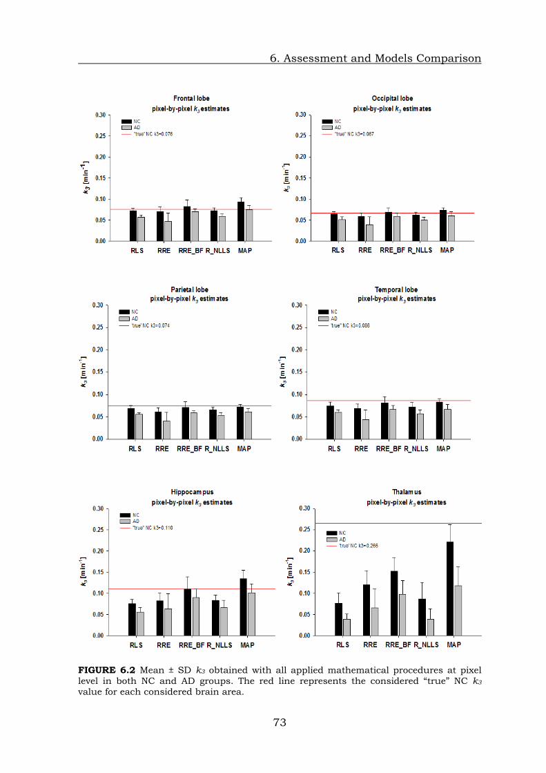
6. Assessment and Models Comparison
FIGURE 6.2 Mean ± SD k3 obtained with all applied mathematical procedures at pixel level in both NC and AD groups. The red line represents the considered “true” NC k3 value for each considered brain area.
73

6. Assessment and Models Comparison
74

7. Discussion
Chapter 7
Discussion
Several recent studies have described in vivo study of AChE activity [1-22].
Reduction of AChE activity was also shown in the cerebral cortex of
patients with Alzheimer disease by quantitative analysis of PET data using 11C-MP4A as tracer [8, 10-16, 19-22]. 11C-MP4A is a ACh analogue and is
specifically hydrolyzed by AChE in the brain to a hydrophilic metabolite,
which is irreversible trapped locally in the brain.
In this study we proposed a new pixel by pixel quantification
approach of brain AChE by PET without arterial blood sampling:
maximum a posteriori parametric estimation (MAP). The standard non
linear least square method was also consider but using reference region
input instead of arterial input function. Comparison with other published
methods based on reference region input (RLS, RRE, RRE_BF), that we
implemented at pixel level, has also been done. As far as we know, a
comparison study at whole brain pixel-by-pixel level for 11C-MP4A
quantification method has not been done yet. Namba and his colleagues
made a tentative of study comparison at pixel level for a temporal area
that covered only 200 pixels for RLS and arterial input NLLS procedure
[22].
Despite the small group of subjects, the mathematical methods
used to generate k3 parametric images in this study, were able to detect
reduction of AChE activity in different brain areas of interest. In
particular, RLS, R-NLLS and MAP analysis identified significant
75

7. Discussion
differences of k3 estimates between NC and AD in regions with low enzyme
expression like temporal, frontal, parietal and occipital cortex, while no
significant differences were identify on neocortex area between NC and AD
groups by applying RRE technique. The performance of RRE and RRE_BF
procedure on our data set is not consistent with that described in the
literature [13, 14, 19]. Therefore it was verified the performance of RRE in
estimating k2 and it was observed inaccurate estimates of this parameter.
In order to consider only reliable parameter estimates, RRE parametric
images have been filtered by calculate a threshold for k2 estimates. The
threshold was estimated in each subject from the k2 parametric image as
the mean k2 value to which was added twice the standard deviation. A
uniform k2 threshold of 2 min-1 was obtained for each person participated
in the study. In this way, only pixels having reliable estimates for RRE
model parameters are taken into account. In case of RRE_BF model that is
based on the same mathematical procedure as RRE but use different
estimation approach of its parameters – basis function – the analysis was
performed three times considering three different conditions for K
parameter (See section 4.3). The k2 threshold was also considered for
RRE_BF analysis in order to have only reliable k3. The significance of the
differences identified in the estimates changes both with K range and
basis function number. Finally, for RRE_BF method has been chosen the
condition that gives estimates closest with the reported literature values.
When applying basis function approach must be considered that for
different neurodegenerative disease might be considered different K range
and different number of basis function that influence the final estimates;
it is also important to be recalled that an underestimation of precision of
estimates are encountered for RRE_BF technique. The reliability of A and
B estimates might also be considered in order to have more reliability in k3
estimates by RRE_BF and RRE.
Significant differences between the groups of subjects were
identified in cerebral region with moderate AChE activity like thalamus by
all mathematical methods. However, if we consider the “true” k3 value of
76

7. Discussion
thalamus from the literature, MAP k3 estimate have the smallest bias
(17%) respect to the “true” value [33]. Ratios of AChE activity values
reported in literature as post mortem human brain ratios were compared
with ratios of k3 values among brain obtained with the analytical methods
applied to our data set. The ratio of AChE activity between the temporal
cortex and thalamus of normal patients obtained with MAP (1:2.7) are
consistent with the same ratio reported in the literature by Arai et al [43]
as a result of a post-mortem human brain study (1:2.7). The same ratios
obtained with the other techniques are much lower (under 1:2).
Brainstem nuclei k3 estimate by MAP method indicate a 50%
reduction in AD AChE activity respect to NC [33]. This data is consistent
with a recently communication in which was reported a reduction of
uptake of the ACh analogue tracer 11C-MP4A in AD subjects who
complained of sleep disturbance [44]. However, no significance between
NC and AD k3 estimates in brainstem nuclei was identify by RLS, R-NLLS,
RRE or RRE_BF analysis.
The automatic extraction of anatomical areas and our comparison
study of the different methodologies for AChE activity quantification at
pixel level confirm that in cortex area with low enzyme activity the models
have similar performances. RRE_BF approach might also be considered
with some cautions. However, RLS linear calculation is faster for pixel by
pixel parameter estimation respect to non linear quantification methods
(R-NLLS, MAP) and the results are in good agreement with cortex values
(FR, TE, PA, OC) already published (see table 6.2).
Contrary, RLS approach showed some difficulties in estimating k3
index in area with moderate enzyme activity. The use of Bayes (MAP)
estimator helps to overcome these drawbacks [33, 34] and allows the
quantification of AChE activity in regions with moderate enzyme
expression at pixel level with results consistent with the scientific
literature [12]. MAP techniques is more time consuming respect to the
other methods because implicate a previous analysis at TAC_ROI level in
order to obtain the a priori information on parameter k2.
77

7. Discussion
78
The results obtained applying mathematical techniques described in
this work at TAC_ROI level showed the smallest differences between
TAC_ROI estimates and pixel estimates for MAP procedure as shown in
chapter 5. However, further work is needed in order to evaluate the
performance of the models on a larger data set. A simulation study based
on real plasmatic data would be very useful in identifying the best non
invasive quantification method for clinical application.

8. Conclusions
Chapter 8
Conclusions 11C-MP4A is a PET tracer that is highly specific for AChE and its kinetic
properties are favorable for the measurement of cortical AChE activity.
Kinetic analysis of 11C-MP4A PET images provides information on the
important physiologic parameter like AChE activity (k3) and about tracer
distribution in different brain areas. The parameter estimates can be used
to derive physiological information as well as to distinguish differences
between various group of subjects, e.g normal and pathological subjects.
The analysis of 11C-MP4A PET images can be performed both at
pixel and region of interest level. In this study some of the recent findings
and issues relative to 11C-MP4A modeling are discussed.
The goal of this study was twofold: first, it was proposed and
developed a Bayesian method (MAP) in order to accurately estimate AChE
activity in normal subjects and patients with neurodegenerative disease
(e.g. AD). A lot of effort was made to ensure accuracy and reliability of all
pixel-level estimates in brain region with low (neocortex) and moderate
(thalamus and brainstem) enzyme activity. The second intent of this work
was to compare, at pixel level, the performance of the Bayesian approach
with the other methods already propose in the literature for AChE activity
quantification: RLS [12], RRE [13], RRE_BF [14], reference NLLS. The
comparison between methods was based on the precision and reliability of
estimates.
In order to avoid errors sampling during a manual position of ROIs
79

8. Conclusions
on the dynamic or parametric 11C-MP4A PET images an automatic ROIs
extraction was preferred to the often used manual technique.
Despite the low number of subjects who participated in the study,
the performance of the various techniques at pixel level showed to be very
similar in the brain areas with low enzyme expression (e. g neocortex).
However, when considering the reliability and accuracy of each models
parameters some issues should be taken into account:
• RLS does not include any information on the measurement
error present in the data, thus does not consider much the
noisiness of the PET study;
• RRE and RRE_BF approaches applied to our data set do not
identified significant differences between NC and AD group
and the results obtained are not in good agreement with
published data. This might be due to the consideration on
error propagation that was implemented in the original
methods or by the selection method used to accept estimates
at pixel level. Another disadvantage of both technique
consisted in inaccurate estimates of the parameter that
describe the unmetabolized tracer washout from tissue to
blood. It is also important to be recalled that an
underestimation of precision of estimates are encountered for
RRE_BF technique.
Anyway, from computational point of view, RLS linear calculation is
faster for pixel by pixel parameter estimation respect to non linear
quantification methods (R-NLLS, MAP) and the results are in good
agreement with published neocortex values.
On the contrary, RLS approach shows some difficulties in estimating
k3 index in area with moderate enzyme activity, such as thalamus and
brainstem. The use of Bayesian (MAP) estimator helps to overcome these
drawbacks and allows the quantification of AChE activity in regions with
moderate enzyme expression, like thalamus and brainstem. At pixel level,
this procedure presents results consistent with the scientific literature.
80

8. Conclusions
MAP technique is more time consuming respect to the other methods
because it implicates a previous analysis at ROI level in order to obtain
the a priori information, but improve the precision of estimates. Actually,
pixel and ROI estimates obtain applying the Bayesian estimator are more
similar respect to the ones obtained with published methods. A new
Bayesian approach that allows a faster identification of the a priori
information is on study. A simulation study based on real plasmatic data
would be very useful for the validation of the best non invasive method.
In conclusion, MAP methods provides the most reliable and accurate
estimates, even if is the most time consuming among the various
procedures.
An European project finalized to validate on a bigger dataset the
best method to be applied to 11C-MP4A/PET images is going to start soon.
Its aim will be the confirmation of the clinical applicability of the chosen
technique in the discrimination of different neurodegenerative pathologies
as AD, Lewy body dementia and mild cognitive impairment. MAP
procedure and another Bayesian method under development as well as
the other non invasive mathematical approach presented in this work will
be taken into account. Real plasma data will also be available for a
simulation study. Thus, simulation results are going to be considered for
best method validation.
81

8. Conclusions
82

Bibliography
Bibliography
[1]. Irie T., Fusushi K., Akimoto Y., Tamagami H., Nozaki T., “Design and
evaluation of radioactive acetylcholine analogs for mapping brain
acetylcholinesterase (AchE) in vivo“ Nucl.Med.Biol (1994), 21:801-
808.
[2]. Irie T, Fusushi K, Namba H, Iyo M, et al, “Brain acetylcholinesterase
activity: validation of a PET tracer in a rat model of Alzheimers
disease”, J Nucl Med (1996), 37: 649-655.
[3]. Namba H, Irie T., Fusushi K, Iyo M, “In vivo measurements of
acetylcholinesterase activity in the brain with radioactive
acetylcholine analog”, Brain.Res. (1994), 667:278-282.
[4]. Kilbourn MR., Snyder SE., Sherman PS., Kuhl DE., “ In vivo studies
of acetylcholinesterase activity using a labeled substrate N-
[11C]methylpiperidin-4-yl propionate ([11C]PMP)“, Synapse, (1996),
22 :123-131.
[5]. Frey KA., Koeppe RA., Kilbourne MR., Snyder SE., Kuhl DE., “PET
quantification of cortical acetylcholinesterase inhibition in monkey
and human“, J. Nucl. Med., (1997), 38:146P.
[6]. Koeppe RA., Frey KA., Snyder SE., Meyer P., Kilbourn MR., Kuhl
DE., “ Kinetic modeling of N-[11C]methylpiperidin-4-yl propionate:
alternatives for analysis of an irreversible PET tracer for measurment
83

Bibliography
of acetylcholinesterase activity in human brain“, Cereb. Blood Flow
Metab., (1999), 19:1150-1163.
[7]. Iyo M, Namba H, Fukushi K, et al, “Measurement of
acetylcholinesterase by positron emission tomography in the brains
of healthy controls and patients with Alzheimer’s disease”, Lancet
(1997), 349: 1805-1809.
[8]. Namba H, Iyo M, Fusushi K, et al., “Human cerebral
acetylcholinesterase activity measured with positron emission
tomography: procedure, normal values and effect of age”, Eur.J Nucl
Med (1999), 26:135-143.
[9]. Kuhl DE, Koeppe RA, Minoshima S, et al.( Kuhl, D. E. MD; Koeppe,
R. A. PhD; Minoshima, S. MD, PhD; Snyder, S. E. PhD; Ficaro, E. P.
PhD; Foster, N. L. MD; Frey, K. A. MD, PhD; Kilbourn, M. R. PhD),
“In vivo mapping of cerebral acetylcholinesterase activity in aging
and Alzheimer’s disease”, Neurology (1999), 52(4): 691-699.
[10]. Herholz K, Bauer B, Wienhard K, et al., “In vivo measurement of
regional acethylcholine esterase activity in degenerative dementia:
comparison with blood flow and glucose metabolism”, J Neural
Transm (2000), 107: 1457-1468.
[11]. Shinotoh H, Namba H, Fusushi K, Nagatsuka S, et al, “Progressive
loss of cortical acetylcholinesterase activity in association with
cognitive decline in Alzheimer’s disease: a positron emission
tomography study”, Ann Neurol (2000), 48: 194-200.
[12]. Nagatsuka S, Fukushi K, Shinotoh H, Namba H, et al., “Kinetic
analysis of [11C]MP4A using a high-radioactivity brain region that
represents an integrated input function for measurement of cerebral
acethylcholinesterase activity without arterial blood sampling”,
JCBFM (2001), 21: 1354-1366.
84

Bibliography
[13]. Herholz K, Lercher M, Wienhard K, Bauer B, Lenz O, Heiss WD, “PET
measurement of cerebral acethylcholine esterase activity without
blood sampling“, Eur J Nucl Med (2001), 28:472-477.
[14]. Zundorf G, Herholz K, Lercher M, Wienhard K, Bauer B, Weisenbach
S, Heiss WD, “PET functional parametric images of acetylcholine
esterase activity without arterial blood sampling” In Senda M et al
(eds), Brain Imaging Using PET, Academic Press, San Diego, Ca,
USA, pp 41-46, Proceedings for BrainPET2001.
[15]. Namba H, Fukushi K, Nagatsuka S, Iyo M, Shinotoh H, Tanada S,
Irie T. “Positron emission tomography: quantitative measurement of
brain acetylcholinesterase activity using radiolabeled substrates.”,
Methods (2002) Jul;27(3):242-50.
[16]. Rinne JO, Kaasinen V, Jarvenpaa T, Nagren K, Roivainen A, Yu M,
Oikonen V, Kurki T., “Brain acetylcholinesterase activity in mild
cognitive impairment and early Alzheimer's disease.”, J Neurol
Neurosurg Psychiatry (2003) Jan;74(1):113-5.
[17]. Herholz K., “PET studies in dementia”, Ann Nucl Med. (2003)
Apr;17(2):79-89.
[18]. Shinotoh H, Fukushi K, Nagatsuka S, Irie T., “Acetylcholinesterase
imaging: its use in therapy evaluation and drug design.”, Curr Pharm
Des. (2004);10(13):1505-17.
[19]. Herholz K, Weisenbach S, Zundorf G, Lenz O, Schroder H, Bauer B,
Kalbe E, Heiss WD, “In vivo study of acetylcholine esterase in basal
forebrain, amygdala, and cortex in mild to moderate Alzheimer
disease.”, Neuroimage (2004) Jan;21(1):136-43.
[20]. Ota T, Shinotoh H, Fukushi K, Nagatsuka S, Namba H, Iyo M,
Aotsuka A, Tanaka N, Sato K, Shiraishi T, Tanada S, Arai H, Irie T.,
“A simple method for the detection of abnormal brain regions in
85

Bibliography
Alzheimer's disease patients using [11C]MP4A: comparison with
[123I]IMP SPECT.”, Ann Nucl Med. (2004) May;18(3):187-93.
[21]. Tsukada H, Nishiyama S, Fukumoto D, Ohba H, Sato K, Kakiuchi T.,
“Effects of acute acetylcholinesterase inhibition on the cerebral
cholinergic neuronal system and cognitive function: Functional
imaging of the conscious monkey brain using animal PET in
combination with microdialysis.”, Synapse. (2004 )Apr;52(1):1-10.
[22]. Namba Hiroki et al, “Pixel-by-pixel Mapping of AChE Activity in
Human Brain with 11C MP4A/PET”, In Senda M et al (eds), Brain
Imaging Using PET, Academic Press, San Diego, Ca, USA, pp 55-61,
Proceedings for BrainPET2001.
[23]. Siegel GJ, Agranoff BW, Albers RW, Fisher SK, Uhler MD, “Basic
Neurochemistry: molecular, cellular and medical aspects“, (Chapter
11), LippincottWilliams&Wilkins, sixth edition, (1999).
[24]. http://wiz2.pharm.wayne.edu/biochem/enz.html, (2007).
[25]. Tanaka N, Fukushi K, Shinotoh H, Nagatsuka S, Namba H, Iyo M,
Aotsuka A, Ota T, Tanada S, Irie T., “Positron emission tomographic
measurement of brain acetylcholinesterase activity using N-
[(11)C]methylpiperidin-4-yl acetate without arterial blood sampling:
methodology of shape analysis and its diagnostic power for
Alzheimer's disease.”, J Cereb Blood Flow Metab. (2001)
Mar;21(3):295-306.
[26]. Walter, B., Blecker, C., Kirsch, P., Sammer, G., Schienle, A., Stark,
R., & Vaitl, D., “MARINA: An easy to use tool for the creation of
MAsks for Region of INterest Analyses” [abstract]. Presented at the
9th International Conference on Functional Mapping of the Human
Brain, June 19-22, (2003), New York, NY. Available CD-Rom in
NeuroImage, Vol. 19, No. 2.
86

Bibliography
[27]. Sato K, Fukushi K, Shinitoh H, Nagatsuka S, Tanaka N, Aotsuka A,
Ota T, Shinraishi T, Tanada S, Iyo M, Irie T, “Evaluation of simplified
kinetic analysis for measurement of brain acetylcholinesterase
activity using N-[11C]Methylpiperidin-4-yl propionate and positron
emission tomography”, JCBFM, (2004), 24:600-611.
[28]. Cobelli C, Carson E, Finkelstein L. “The mathematical Modeling of
Metabolic and Endocrine System”. New York, Wiley (1983).
[29]. http://en.wikipedia.org/wiki/Maximum_a_posteriori,(2007)
[30]. Bertoldo, A., Sparacino, G., Cobelli, C., “Population approach
improves parameter estimation of kinetic models from dynamic PET
data”, IEEE Trans.Med.Im, (2004); 23(3):297-306.
[31]. Sparacino, G., Tombolato, C., Cobelli, C, “Maximum Likelihood
versus Maximum a posteriori parameter estimation of physiological
system models:the C-peptide impulse response case study”., IEEE
Trans.BioMed.Eng, (2000); 47(6):801-811.
[32]. Callegari, T., Caumo A., Cobelli, C., “Generalization of Map
estimation in SAAM II: validation against ADAPT II in a glucose
model case study”, Ann.BioMed.Eng., (2002); 30:1-8.
[33]. Florea I., Bertoldo A., Moresco RM, Carpinelli A, Panzacchi A,
Garibotto V, Perani D, Gilardi MC, Fazio F, Cobelli C., “[11C] MP4A
Bayesian quantification of AChE activity at pixel and ROI level in
normals and Alzheimer patients.”, Proceedings of 2nd European
Society of Molecular Imaging, Naples, Italy, 14 - 15 June (2007). [34]. Florea I., Bertoldo A., Pietra L., Moresco RM, Carpinelli A, Panzacchi
A, Garibotto V, Perani D, Gilardi MC, Fazio F, Cobelli C., “Kinetic
analysis of [11C]MP4A for measurement of cerebral acetylcholine
esterase activity without arterial blood sampling.”, Proceedings for
87

Bibliography
6th International Symposium on Functional Neuroceptor Mapping,
Copenhagen – Denmark, 6th - 8th July (2006). [35]. http:// en.wikipedia.org/wiki/Acetylcholine, (2007).
[36]. http://www.pharmacorama.com/en/Sections/Acetylcholine.php,
(2007).
[37]. http://www.cnsforum.com/imagebank/section/Dementia_Cholinerg
ic/default.aspx, (2007).
[38]. www.dns.ed.ac.uk/teaching.html, (2007).
[39]. http://www.mrothery.co.uk/studentswork/synapses%20and%20dru
gs.ppt#260, (2007).
[40]. Purves, Dale; Augustine, George J.; Fitzpatrick, David; Katz,
Lawrence C.; LaMantia, Anthony-Samuel; McNamara, James O.;
Williams, S. Mark., Neuroscience Sunderland (MA): Sinauer
Associates, Inc. ; (c2001).
[41]. Herholz K., Heiss, W.D., “Positron Emission Tomography in Clinical
Neurology”, Molecular Imag. Biol, (2004), 6(4):239-269.
[42]. Carpinelli A, Magni F, Cattaneo A, Matarrese M, Turolla E, Todde S,
Bosso N, Galli Kienle M, Fazio F., “Improved synthesis and
radiolabeling of [11C]MP4A, a suitable ligand for the investigation of
the cholinergic system using PET“, Appl Radiat Isot. (2006)
Feb;64(2):182-6.
[43]. Arai H., Kosaka k., Muramoto O., Moroji T., Iizuka R., ”A biochemical
study of cholinergic neurons in the post mortem brains from the
patient with alzheimer-type dementia.” Clin Neurol (Tokyo)(1984);
24:1128-1135.
88

Bibliography
[44]. Eggers C, Szelies B, Bauer B, Wienhard K, Schroder H, Herholz K,
Heiss WD., “Imaging of acetylcholine esterase activity in brainstem
nuclei involved in regulation of sleep and wakefulness“, Eur J Neurol.
(2007) Jun;14(6):690-3.
[45]. Lammertsma A. and Hume S. P., “Simplified reference tissue model
for pet receptor studies”, NeuroImage, ( 1996) 4, 153-58.
[46]. Blumqvist G., “ On the construction of functional maps in positron
emission tomography”, J. Cereb. Blood Flow Metab, (1984), 4:629-
632
[47]. Carson E., Cobelli C “Modelling methodology for physiology and
medicine”, Academis Press, San Diego, CA, USA, (2001).
[48]. Koeppe RA, Frey KA, Snyder SE, Kuhl DE, “Kinetic modeling of N-
[11C]methylpiperidin-4-yl propionate: alternatives for analysis of an
irreversible positron emission tomography trace for measurement of
acetylcholinesterase activity in human brain”, J Cereb Blood Flow
Metab., (1999) ,19(10):1150-63.
[49]. Mesulam MM, Geula C, “Acetylcholinesterase-rich neurons of the
human cerebral cortex: cytoarchitectocnic and ontogenetic patterns
of distribution”, J. Comp Neurol (1991), 306: 193-220.
[50]. Mesulam MM, Geula C, “Overlap between acetylcholinesterase-rich
and cholin acetyltransferase-positive (cholinergic) axons in human
cerebral cortex”, Brain Res, (1992), 577: 112-120.
[51]. Geula C, Mesulam MM, “Cholinergic systems and related
neuropathological predilection patterns in Alzheimer disease”, in
Terry RD, et al(eds) Alzheimer Disease, Raven Press, New York,
(1994), pp 263-291.
89

Bibliography
90

Acknowledgments It was a pleasure for me to work with all the wonderful people from Padua
University and from PET Unit of San Raffaele Hospital in Milan.
First of all, I would like to thank Prof. Claudio Cobelli and Prof. Maria
Carla Gilardi for their support and for giving me the chance to visit several
interesting conferences.
A special thank to Dr. Alessandra Bertoldo. Her ideas and support had a
major influence on this thesis. She spent a lot of time advising me: I
learned a lot during this time and I am convinced that this knowledge will
help me in the future.
Many thanks to Dr. Rosamaria Moresco that was so kind during my
permanence in Milan group. I am happy to have had such a supportive
collaborator.
I would like to thank Karl Herholz, MD for reviewing my thesis. I enjoyed
his interest in my research as well as his useful suggestion.
My thanks to Dr. Andrea Caumo, a wonderful friend and collaborator:
thank you for sharing with me the wonderful world of mathematical
modeling for biological system.
My thanks to my friends and colleagues from Padua for the great time I
had in the group. I enjoyed the atmosphere, their friendship, and their
91

92
support. Thank you all. A special thank to my dear friend Giulia for her
friendship, hospitality and almost daily sharing.
My thanks to my friend and colleagues from Milan for the great
collaboration over the years (especially for your understanding in the last
month of my PhD). It was a pleasure to work with all these people and to
benefit from their knowledge. Especially, I would like to thank Giovanna
for the “brainstorming” in moments of engineering doubts. Many thanks to
Lorena, for the wonderful technical support and for lifetime discussion.
And thank you Deby, Dany and all of you guys that shared lunch,
coffee/tea break and for the cool time we had at LITA.
Additionally, I would like to thank several people that encourage me
always: my friends Anna and Marco(*2), Andreia and Tudor.
My grateful thanks to my family who supported me with all I have done
during my life. Thank you Mama, Toto, Mami, Tati: you are always in my
thoughs and heart. My thanks for my parents in low for their love and
support.
Last but not least, I wish to thank my husband Anto for always loving,
supporting me and for enjoying life together with me.