Embed Size (px)
Citation preview
UniversitatAutònomade Barcelona
Exploring Arterial Dynamics andStructures in IntraVascular UltraSound
Sequences
A dissertation submitted by Aura Hernandezi Sabate at Universitat Autonoma de Barcelonato fulfil the degree of Doctora en Informatica.
Bellaterra, July 2009

Director: Dra. Debora Gil ResinaUniversitat Autonoma de BarcelonaDep. Ciencies de la Computacio i Centre de Visio per Computador
Centre de Visióper Computador
This document was typeset by the author using LATEX2ε.
The research described in this book was carried out at the Computer Vision Center,Universitat Autonoma de Barcelona.
Copyright c© 2009 by Aura Hernandez i Sabate. All rights reserved. No partof this publication may be reproduced or transmitted in any form or by any means,electronic or mechanical, including photocopy, recording, or any information storageand retrieval system, without permission in writing from the author.
Good use right: it is strictly prohibited to use, to investigate or to develop, in adirect or a indirect way, any of the scientific contributions of the author contained inthis work by any army or armed group in the world, for military purposes and for anyother use which is against human rights or the environment, unless a written consentof all the persons in the world is obtained.
ISBN 978-84-937261-6-4
Printed by Ediciones Graficas Rey, S.L.

Al Lluıs i els meus paresGracies per ser-hi sempre


Agraıments
L’obtencio del tıtol de doctora implica assolir el grau academic mes alt. Ja he acabatd’estudiar? Potser des del punt de vista academic sı, pero segurament no des de capaltre. Durant aquests 6 anys, que es compliran el dia que defensi aquest treball, heapres moltıssimes coses a nivell academic, pero tambe a molts altres nivells, sobretotel personal. Ha estat una etapa que s’ha fet llarga a epoques i molt curta a d’altres.
Una etapa amb llargues hores de discussio per intentar que el mon de les ecografiesintra-coronaries, entre d’altres, sigui una mica mes planer. Hores en que la foscorsemblava guanyar terreny i hores en que el cel era a tocar. Pero per sobre de tot,hores de dedicacio i entusiasme on he apres que la intuıcio i la perseveranca et portenper bons camins. Una etapa acompanyada de tot tipus de persones. Persones quem’han transmes la seva passio per la investigacio. Persones que sempre tenen unmoment per discutir de qualsevol cosa, ja sigui sobre metodes de comparacio multipleo de si els de l’obra del davant posen en perill les nostres vides. Hores tambe dedespatx on, a part de treballar i discutir si es millor el windows o el linux, hem fetpessebres, hem rigut, ens hem renyat i hem discutit sobre el nostre futur. He conviscutel dia a dia amb grans persones, que m’han ensenyat a respectar mes els altres, quem’han cuidat en els moments baixos i que m’han enriquit amb les seves visions de lavida.
Aquesta etapa tambe ha tingut les seves hores de docencia. Hores en contacte ambalumnes de 20 anys (i alguns mes), que et contagien les ganes de menjar-se el mon iet recorden que la vida son dos dies i que cal viure-la. Pero les classes no haguessinestat les mateixes sense la preparacio previa. Preparacio enriquida amb els diferentspunts de vista sobre la filosofia docent. Intercanvis d’opinions varies sobre quin es elmillor metode a seguir perque els alumnes aprenguin, perque no copiın, perque no esrebel·lin... i no oblidem les batalletes explicades pels mes experts en la materia, dequi s’apren mes!
Totes aquestes hores, a vegades mes de les que toca, han ocupat la meva jornadalaboral. I moltes hores tambe han estat fora d’aquesta, ja sigui a l’hora de dinar ofent un cafe. Pero a l’hora de dinar intentem desconnectar de la recerca i la docenciai riure una mica del veı. D’aixo se n’han encarregat molt be alguns grans amics i unesbones orelles. Alguns han vingut mes tard, altres ja han marxat, altres han vingut depas i altres venen de tant en tant, pero el requisit principal es saber riure de qualsevolcosa i voler passar una bona estona. Al cap i a la fi, darrere d’aquests escarnis hi hamales persones que van de bones persones que van de males persones. O no era aixı?!
I tambe han estat molts cigarrets! Tot i que fa mes d’un any que no fumo, ha
i

ii AGRAIMENTS
estat molt quitra consumit, controlant les obres i arreglant el mon, sempre molt benacompanyada de persones que, com jo, buscaven 10 minuts per respirar ”aire pur”.Persones que m’han animat a posar aquests agraıments. Persones que, tot i no fumar,m’acompanyaven mentre feien el cafe, tot mostrant-me amb les seves experiencies quela vida no es en blanc i negre, sino que te 256 nivells de gris i cal pensar en el futur.Amics que saben apreciar una bona caminada pel campus i una bona xocolata i quesaps que son alla en moments importants de la teva vida.
Resumint, durant aquests anys he conegut i retrobat grans persones. Persones quehan confiat en mi. Persones que m’han fet riure i persones que m’han fet plorar. Per-sones que sorprenen i persones que apareixen quan menys t’ho esperes. En definitiva,persones que no m’han deixat indiferent al llarg d’aquesta etapa i que m’han ajudat,d’una manera o d’una altra, a creixer en molts aspectes.
Pero abans d’aquesta etapa ja hi havia grans persones. Amigues que encara nosaben exactament el que faig o que creuen que perdo el temps, pero que tot i aixı emdonen suport sempre que el necessito i comparteixen les meves alegries sempre quees pot. Familiars que creuen que faig coses molt rares o que gracies a mi no es volendedicar al mon de la investigacio, pero que tambe estan alla quan cal, ja sigui perescoltar o per celebrar. Com a familiar especial he de parlar del meu fill adoptiu, quetambe ha estat pels detalls matematics que jo ja he oblidat o per escoltar-me quanes necessari. I no m’oblido de les persones mes importants de la meva vida fins almoment, els meus pares i el Lluıs, que han cregut en mi des del primer moment i hantingut la paciencia d’escoltar-me i aguantar-me durant tots aquests anys.
Es per tot aixo que us dono les gracies a totes les persones que, en els momentsmes baixos d’aquesta historia, heu estat alla, d’una forma o una altra, pero tambe atotes les que heu sabut gaudir dels seus moments algids i heu compartit amb mi laseva celebracio.

Resum
Les malalties cardiovasculars son una de les principals causes de mortalitat als paısosdesenvolupats. La majoria d’elles son degudes a malalties arterials (especialment lescoronaries), que venen causades per l’acumulacio de placa. Aquesta patologia es-treny el flux sanguini (estenosi) i afecta les propietats elastiques i bio-mecaniques(arteriosclerosi) de les arteries. En les ultimes decades, l’Ecografia Intra-Coronaria(EIC) ha esdevingut una tecnica usual de diagnostic per la imatge i seguiment de lesmalalties coronaries. L’EIC esta basada en un cateterisme que mostra una sequenciad’imatges corresponents a seccions de l’arteria sota estudi. La inspeccio visual decadascuna d’aquestes imatges proporciona informacio sobre el percentatge d’estenosi,mentre que la inspeccio de les vistes longitudinals propociona informacio sobre lespropietats bio-mecaniques, que pot prevenir un desenllac fatal de la malaltia cardio-vascular. Per una banda, la dinamica arterial (deguda al batec del cor, entre d’altres)es un dels principals artefactes per poder explorar les propietats biomecaniques. Almateix temps, les mesures manuals d’estenosi requereixen un tracat manual de lesvores del vas, tasca feixuga que consumeix molt de temps i que pot patir variabilitatentre observadors.
Aquesta tesi proposa varies eines de processament d’imatge per explorar la dinamicade les arteries i les seves estructures. Presentem un model fısic per extreure, analitzari corregir la dinamica rıgida transversal dels vasos i per recuperar la fase cardıaca.A mes, introduım un metode estadıstic-determinista per a la deteccio automatica deles vores del vas. En particular, l’enfoquem a segmentar l’adventıcia. Un protocol devalidacio acurat per assegurar una aplicacio clınica fiable del metodes es un pas crucialen qualsevol proposta d’algorisme. En aquesta tesi tenim especial cura de dissenyarprotocols de validacio per a cadascuna de les tecniques proposades i contribuım a lavalidacio de la dinamica in vivo amb un indicador objectiu i quantitatiu per mesurarla quantitat de moviment suprimida.
iii

iv RESUM

Abstract
Cardiovascular diseases are a leading cause of death in developed countries. Most ofthem are caused by arterial (specially coronary) diseases, mainly caused by plaqueaccumulation. Such pathology narrows blood flow (stenosis) and affects artery bio-mechanical elastic properties (atherosclerosis). In the last decades, IntraVascularUltraSound (IVUS) has become a usual imaging technique for the diagnosis and followup of arterial diseases. IVUS is a catheter-based imaging technique which shows asequence of cross sections of the artery under study. Inspection of a single image givesinformation about the percentage of stenosis. Meanwhile, inspection of longitudinalviews provides information about artery bio-mechanical properties, which can preventa fatal outcome of the cardiovascular disease. On one hand, dynamics of arteries (dueto heart pumping among others) is a major artifact for exploring tissue bio-mechanicalproperties. On the other one, manual stenosis measurements require a manual tracingof vessel borders, which is a time-consuming task and might suffer from inter-observervariations.
This PhD thesis proposes several image processing tools for exploring vessel dy-namics and structures. We present a physics-based model to extract, analyze andcorrect vessel in-plane rigid dynamics and to retrieve cardiac phase. Furthermore, weintroduce a deterministic-statistical method for automatic vessel borders detection.In particular, we address adventitia layer segmentation. An accurate validation pro-tocol to ensure reliable clinical applicability of the methods is a crucial step in anyproposal of an algorithm. In this thesis we take special care in designing a valida-tion protocol for each approach proposed and we contribute to the in vivo dynamicsvalidation with a quantitative and objective score to measure the amount of motionsuppressed.
v

vi ABSTRACT

Contents
Agraıments i
Resum iii
Abstract v
Introduction 1IntraVascular UltraSound Imaging . . . . . . . . . . . . . . . . . . . . 1Goal of the Thesis . . . . . . . . . . . . . . . . . . . . . . . . . . . . . 6Vessel Dynamics Exploring . . . . . . . . . . . . . . . . . . . . . . . . 7
Our Contribution - Physics-based models . . . . . . . . . . . . 8Vessel Structures Segmentation . . . . . . . . . . . . . . . . . . . . . . 9
Our Contribution - A Deterministic-Statistical Strategy . . . . 10Validation Protocols . . . . . . . . . . . . . . . . . . . . . . . . . . . . 11
Our Contribution - In-vivo Protocol Design . . . . . . . . . . . 12
1 Theoretical Issues 151.1 Affine Maps . . . . . . . . . . . . . . . . . . . . . . . . . . . . . . . . . 15
1.1.1 Affine Transformations in Polar Coordinates . . . . . . . . . . 181.2 Fourier Transform . . . . . . . . . . . . . . . . . . . . . . . . . . . . . 20
1.2.1 Properties . . . . . . . . . . . . . . . . . . . . . . . . . . . . . . 221.2.2 Particular Cases of Fourier Transforms . . . . . . . . . . . . . . 24
1.3 Anisotropic Restricted Operators . . . . . . . . . . . . . . . . . . . . . 261.3.1 Structure-Preserving Diffusion . . . . . . . . . . . . . . . . . . 271.3.2 Anisotropic Contour Closing . . . . . . . . . . . . . . . . . . . 28
1.4 B-snakes . . . . . . . . . . . . . . . . . . . . . . . . . . . . . . . . . . . 301.5 Proofs . . . . . . . . . . . . . . . . . . . . . . . . . . . . . . . . . . . . 32
2 Physics-based Models for Vessel Dynamics Exploring 352.1 In-plane Dynamics . . . . . . . . . . . . . . . . . . . . . . . . . . . . . 36
2.1.1 Translation . . . . . . . . . . . . . . . . . . . . . . . . . . . . . 362.1.2 Rotation . . . . . . . . . . . . . . . . . . . . . . . . . . . . . . . 402.1.3 Dynamics Decomposition . . . . . . . . . . . . . . . . . . . . . 42
2.2 Longitudinal Dynamics . . . . . . . . . . . . . . . . . . . . . . . . . . 442.2.1 Step 1 - Extraction of Signal Reflecting Cardiac Motion . . . . 45
vii

viii CONTENTS
2.2.2 Step 2 - Signal Filtering for Cardiac Profile Extraction . . . . . 472.2.3 Step 3 - Retrieval of Cardiac Phase . . . . . . . . . . . . . . . . 49
2.3 Mathematical Issues . . . . . . . . . . . . . . . . . . . . . . . . . . . . 50
3 Deterministic-Statistical Strategies for Structures Exploring 553.1 General Strategy . . . . . . . . . . . . . . . . . . . . . . . . . . . . . . 553.2 Step 1 - Image Preprocessing . . . . . . . . . . . . . . . . . . . . . . . 57
3.2.1 Polar Coordinates . . . . . . . . . . . . . . . . . . . . . . . . . 573.2.2 Image Filtering . . . . . . . . . . . . . . . . . . . . . . . . . . . 58
3.3 Step 2 - Statistical Selection of Border Points . . . . . . . . . . . . . . 593.3.1 Feature Space Design . . . . . . . . . . . . . . . . . . . . . . . 603.3.2 Statistical Parameter Setting . . . . . . . . . . . . . . . . . . . 62
3.4 Step 3 - Closing Stage . . . . . . . . . . . . . . . . . . . . . . . . . . . 663.4.1 Anisotropic Contour Closing . . . . . . . . . . . . . . . . . . . 663.4.2 B-snakes . . . . . . . . . . . . . . . . . . . . . . . . . . . . . . . 67
3.5 Numerical Issues . . . . . . . . . . . . . . . . . . . . . . . . . . . . . . 683.5.1 Parameters Tuning . . . . . . . . . . . . . . . . . . . . . . . . . 693.5.2 Quick ACC . . . . . . . . . . . . . . . . . . . . . . . . . . . . . 70
4 Validation Protocols 734.1 In-plane Dynamics . . . . . . . . . . . . . . . . . . . . . . . . . . . . . 73
4.1.1 Conservation of Density Rate . . . . . . . . . . . . . . . . . . . 734.1.2 Ground Truth . . . . . . . . . . . . . . . . . . . . . . . . . . . . 764.1.3 Goodness Measures . . . . . . . . . . . . . . . . . . . . . . . . 78
4.2 Longitudinal Dynamics . . . . . . . . . . . . . . . . . . . . . . . . . . 794.2.1 Ground Truth . . . . . . . . . . . . . . . . . . . . . . . . . . . . 794.2.2 Goodness Measures . . . . . . . . . . . . . . . . . . . . . . . . 79
4.3 Vessel Structures . . . . . . . . . . . . . . . . . . . . . . . . . . . . . . 834.3.1 Ground truth . . . . . . . . . . . . . . . . . . . . . . . . . . . . 834.3.2 Goodness Measures . . . . . . . . . . . . . . . . . . . . . . . . 83
5 Experiments 875.1 In-plane Dynamics . . . . . . . . . . . . . . . . . . . . . . . . . . . . . 87
5.1.1 Synthetic Data . . . . . . . . . . . . . . . . . . . . . . . . . . . 875.1.2 In vivo Data . . . . . . . . . . . . . . . . . . . . . . . . . . . . 90
5.2 Longitudinal Dynamics . . . . . . . . . . . . . . . . . . . . . . . . . . 915.3 Vessel Structures . . . . . . . . . . . . . . . . . . . . . . . . . . . . . . 945.4 Discussion . . . . . . . . . . . . . . . . . . . . . . . . . . . . . . . . . . 102
Conclusions and Further Lines 105Further Lines . . . . . . . . . . . . . . . . . . . . . . . . . . . . . . . . 106
Publications 107
Bibliography 109

List of Tables
4.1 F Distribution critical values for α = 0.1 . . . . . . . . . . . . . . . . . 814.2 F Distribution critical values for α = 0.05 . . . . . . . . . . . . . . . . 824.3 Critical values for the two-tailed Nemenyi test . . . . . . . . . . . . . . 824.4 Critical values for the two-tailed Bonferroni-Dunn test. The number
of methods include the control method . . . . . . . . . . . . . . . . . . 83
5.1 Angle Absolute Error Ranges for Synthetic Profiles - Static Model . . 875.2 Angle Absolute Error Ranges for Synthetic Profiles - Sequence Model 875.3 Absolute Error Ranges for in vivo Profiles. . . . . . . . . . . . . . . . 885.4 CDR vs Angle Relative Error . . . . . . . . . . . . . . . . . . . . . . . 895.5 CDR vs Other Alignment measures . . . . . . . . . . . . . . . . . . . . 895.6 Average Rank of the Gaussian Filters with parameters given by σ for
Nemenyi Test . . . . . . . . . . . . . . . . . . . . . . . . . . . . . . . . 915.7 Average Rank of the Butterworth Filters with parameters given by
(n, δ) for Nemenyi Test . . . . . . . . . . . . . . . . . . . . . . . . . . . 915.8 Average Errors of the best set of filters . . . . . . . . . . . . . . . . . . 925.9 Performance Evaluation of the Adventitia Segmentation Strategy. Au-
tomatic Errors versus Inter-Observer Variability for non-calcified . . . 955.10 Performance Evaluation of the Adventitia Segmentation Strategy. Au-
tomatic Errors versus Inter-Observer Variability for calcified segments 965.11 Performance Evaluation of the Adventitia Segmentation Strategy. Au-
tomatic Errors versus Inter-Observer Variability for all segments . . . 965.12 Statistics Summary on T-tests comparing the means of Inter-Observer
Variability and Automatic Errors. . . . . . . . . . . . . . . . . . . . . 97
ix

x LIST OF TABLES

List of Figures
1 Images extracted from an IVUS pullback . . . . . . . . . . . . . . . . . 22 IntraVascular UltraSound single image inspection . . . . . . . . . . . . 33 Longitudinal Cut of an IVUS Sequence . . . . . . . . . . . . . . . . . . 44 Swinging effect in longitudinal cuts . . . . . . . . . . . . . . . . . . . . 55 Artifacts in longitudinal cut appearance induced by in-plane dynamics. 66 Pipeline for Image-based Cardiac Phase Retrieval . . . . . . . . . . . . 7
1.1 Affine Coordinates . . . . . . . . . . . . . . . . . . . . . . . . . . . . . 161.2 Affine Transformation . . . . . . . . . . . . . . . . . . . . . . . . . . . 171.3 IVUS image in Cartesian and polar coordinates . . . . . . . . . . . . . 191.4 Rotation in polar coordinates . . . . . . . . . . . . . . . . . . . . . . . 191.5 Phase and amplitude of a wave . . . . . . . . . . . . . . . . . . . . . . 211.6 Image filtering in the Fourier domain . . . . . . . . . . . . . . . . . . . 231.7 Shifted Functions . . . . . . . . . . . . . . . . . . . . . . . . . . . . . . 241.8 Fourier transforms of periodic and non-periodic functions . . . . . . . 251.9 Vector field representing level curves of an angiography for a vessel and
a background structure-less area . . . . . . . . . . . . . . . . . . . . . 281.10 Performance of smoothing approaches on cardiac magnetic resonance
images. . . . . . . . . . . . . . . . . . . . . . . . . . . . . . . . . . . . 291.11 Anisotropic Contour Closing . . . . . . . . . . . . . . . . . . . . . . . . 30
2.1 Adventitia Straighten Procedure . . . . . . . . . . . . . . . . . . . . . 382.2 Detection of points roughly lying on the adventitia for different mor-
phologies . . . . . . . . . . . . . . . . . . . . . . . . . . . . . . . . . . 392.3 Center of gravity computations . . . . . . . . . . . . . . . . . . . . . . 392.4 Regression plane approximating Fourier phase correlation between two
shifted images. . . . . . . . . . . . . . . . . . . . . . . . . . . . . . . . 412.5 Motion Decomposition into geometric, breathing and cardiac terms . . 442.6 Pipeline for Image-based Cardiac Phase Retrieval . . . . . . . . . . . . 452.7 First Selection of pixels reflecting motion along the sequence . . . . . 462.8 Regular Profile versus irregular profile . . . . . . . . . . . . . . . . . . 472.9 Final selection of points reflecting cardiac motion . . . . . . . . . . . . 472.10 Butterworth filters for different parameters . . . . . . . . . . . . . . . 482.11 Gaussian filters for different parameters . . . . . . . . . . . . . . . . . 48
xi

xii LIST OF FIGURES
2.12 Signal filtering with a Butterworth filter with parameters n = 2; δ = 0.1 492.13 Comparison between point clouds in the case of a pure rotation and a
rotation perturbed by a scaling for two different morphologies, calciumand soft plaque . . . . . . . . . . . . . . . . . . . . . . . . . . . . . . . 51
2.14 Relation between perturbation and error in translation. . . . . . . . . 52
3.1 Adventitia images in cartesian and polar coordinates . . . . . . . . . . 573.2 Scheme of the strategy for approaching the geometric center of mass . 583.3 Image SPD Filtering . . . . . . . . . . . . . . . . . . . . . . . . . . . . 593.4 Stabilized Sequence Filtering . . . . . . . . . . . . . . . . . . . . . . . 603.5 Image descriptors: Horizontal Edges, Radial Standard Deviation and
Cumulative Radial Mean . . . . . . . . . . . . . . . . . . . . . . . . . . 623.6 Adventitia/Intima vs Calcium/Fibrous Tissue sets Discrimination . . 643.7 Vessel Borders Point Extraction (1). Adventitia mask resulting from
the classification and the final one after length filtering . . . . . . . . . 653.8 Precision-Recall curve to select thresholding values for the computation
of calcium mask . . . . . . . . . . . . . . . . . . . . . . . . . . . . . . . 663.9 Vessel Borders Point Extraction (2). Calcium mask . . . . . . . . . . . 663.10 Adventitia Closing Step . . . . . . . . . . . . . . . . . . . . . . . . . . 693.11 Maximum Absolute Error function for Length and Area Filtering Pa-
rameters . . . . . . . . . . . . . . . . . . . . . . . . . . . . . . . . . . . 713.12 Mean Absolute Error function for Length and Area Filtering Parameters 723.13 Quick Anisotropic Contour Closing. . . . . . . . . . . . . . . . . . . . 72
4.1 Quality Measure Computation . . . . . . . . . . . . . . . . . . . . . . 754.2 Manual Sampling for a Sequence . . . . . . . . . . . . . . . . . . . . . 79
5.1 Box plots for the sequence-based phantoms and a representative imageof the sequence for each phantom . . . . . . . . . . . . . . . . . . . . . 88
5.2 Linear Correlation between CDR and Angle Relative Accuracy (ε13). . 89
5.3 Longitudinal cuts for sequences of four different patients, from the bestcorrected sequence to the worst corrected one . . . . . . . . . . . . . . 90
5.4 Comparison of different filters using the Nemenyi test. . . . . . . . . . 925.5 Image-based ECG sampling on a longitudinal cut. . . . . . . . . . . . 935.6 Results of Image-based ECG sampling for two different longitudinal
cuts. . . . . . . . . . . . . . . . . . . . . . . . . . . . . . . . . . . . . 935.7 Whisker Boxes for Automated Error and Inter-Observer Variability . . 955.8 Automated Adventitia Detections for Normal Vessel Segments . . . . . 985.9 Automated Adventitia Detections for Vessel Segments with Soft Plaque 995.10 Automated Adventitia Detections for Calcified Vessel Segments . . . . 1005.11 Automated Adventitia Detections for Uncomplete Vessel Segments . . 1015.12 Adventitia models in images with sparse information . . . . . . . . . . 103

Introduction
There is general consensus that cardiovascular diseases (cerebrovascular, peripheralarterial, coronary heart, and strokes among others) are a leading cause of death.According to the World Health Organization1, they constitute approximately a 30%of all global deaths and they are projected to remain the single leading causes ofdeath. Among cardiovascular diseases, coronary heart pathologies (which can triggeranginas and heart strokes, for instance) constitute the gross of these deaths with a33%.
Artery diseases are mainly caused by the accumulation of plaque (made up of acombination of blood cholesterol, fat and cells) inside arterial walls [1]. Such plaqueaccumulation narrows the artery’s blood flow (stenosis) and makes arteries inflamingand being less flexible (atherosclerosis). Artery blood flow reduction is measured bythe percentage of obstruction in vessel sections and is a usual measurement previ-ous to decide which is the best treatment (either surgical or pharmacological) for anatherosclerotic lesion. Depending on the histological composition of the plaque, its(bio-mechanical) physical behavior will be different, making it more or less unsta-ble (vulnerable plaques) and, thus, resulting in a different risk for the patient [2].Early detection of plaque composition is a main step for planning the most suitabletreatment (angioplasty, stent apposition, ...) and might prevent further thrombosispotentially leading to a fatal heart attack. Tissue bio-mechanical properties play animportant role in the diagnosis and treatment of cardiovascular diseases. The mainmechanical properties currently under study are radial strain, which is related toplaque type and vulnerability [3], and shear stress, which influences the probabilityof plaque accumulation [4]. Both measures can be computed by means of the studyof vessel tissue deformation along the cardiac cycle.
IntraVascular UltraSound Imaging
IntraVascular UltraSound (IVUS) [5] is a wide used catheter-based technique whichprovides cross-sectional views of the artery. A guide wire with a catheter inside isthreaded through the coronary artery under study. A catheter is composed of a RadioFrequency (RF) emitter and a transducer. The RF emitter sends ultrasound waveswhose beams are reflected on arterial tissue particles and collected by the transducer.Images are reconstructed from the reflection of this signal, so, its grey level is related to
1www.who.int
1
2 INTRODUCTION
tissue density of mass [6,7]. The catheter is mechanically pulled back with a constantvelocity (usually at 0.5 mm/s) along the artery providing a sequence (digitized at20-30 frames per second) of IVUS images.
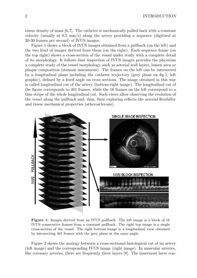
Figure 1 shows a block of IVUS images obtained from a pullback (on the left) andthe two kind of images derived from them (on the right). Each sequence frame (onthe top right) shows a cross-section of the vessel under study with a complete detailof its morphology. It follows that inspection of IVUS images provides the physiciana complete study of the vessel morphology, such as arterial wall layers, lumen area orplaque composition (stenosis assessment). The frames on the left can be intersectedby a longitudinal plane including the catheter trajectory (grey plane on fig.1, leftgraphic), defined by a fixed angle on cross sections. The image obtained in this wayis called longitudinal cut of the artery (bottom-right image). The longitudinal cut ofthe figure corresponds to 401 frames, while the 16 frames on the left correspond to athin stripe of the whole longitudinal cut. Such views allow observing the evolution ofthe vessel along the pullback and, thus, their exploring reflects the arterial flexibilityand tissue mechanical properties (atherosclerosis).
Figure 1: Images derived from an IVUS pullback. The left image is a block of 16IVUS consecutive frames from a constant pullback. The right top image is a singlecross-section of the vessel. The right bottom image is a longitudinal view obtainedby intersecting 401 frames with the grey plane at the same angle.
Figure 2 shows the analogy between a cross-sectional histological cut of an artery(left image) and the corresponding IVUS image (right image). In muscular arteries,like coronary arteries, there are frequently three layers [8]. The innermost layer con-

3
Figure 2: IntraVascular UltraSound single image inspection. On the left, a cross-sectional histological cut of the vessel with its most frequent vessel structures. Onthe right, its corresponding cross-sectional IVUS image.
sists of a set of three elements: intima, atheroma (in diseased vessels), and internalelastic membrane. Moving outward from the lumen (the inside space where bloodflows), the second layer is the media, which is usually less homogeneous than the in-tima. The third and outer layer consists of the adventitia and peri-adventitial tissues.The membrane separating the second and the third layers corresponds to the exter-nal elastic membrane (EEM). Vessel plaque accumulates between intima and media.Depending on the disease of the artery, there exist different kind of plaques: calcified,soft, fibrous, and mixed plaque. On the right side of figure 2 we have the visualizationof the layers and plaque in an IVUS cross-section. The contour between lumen andintima, depicted in red, corresponds to the internal elastic membrane. The trailingedge of the intima cannot always be distinguished clearly because in some cases themedia may appear artifactually thin because of an intense reflection from the intimaor external elastic membrane. In the IVUS image of fig.2, the intima-media layer isnot visible. However, a discrete interface at the border between the media and theadventitia is almost invariably present within IVUS images and corresponds closelyto the location of the EEM, which is colored in yellow. There is no distinct boundaryon IVUS images separating the true adventitia from surrounding perivascular tissues.Regarding plaque, its intensity increases proportionally to its density of mass, so that,soft, fibrous and calcium appear with increasing brightness. In the IVUS image offig.2, there is a calcified plaque (colored in green) in the second quadrant. The differ-ential feature of calcium is the echo shadow behind it due to its echo opacity. Anothershadow usually observed in an IVUS image is the artifact produced by the guide wirereflection (in the fourth quadrant of the image).
The qualitative description of the artery provided by IVUS images enables the

4 INTRODUCTION
assessment of several measurements such as stenosis, EEM and lumen areas. Thepercentage of stenosis is computed as the ratio between the area of the lumen and thearea of the EEM times 100. Lumen measurements are performed using the interfacebetween the lumen and the leading edge of the intima. All these measurements re-quire an accurate segmentation of vessel borders for the whole sequence block. For asegment of 25 mm. long, it implies exploring about 5000-7500 frames (depending onthe frame rate) in a standard intervention. Such huge amount of frames implies thatan exhaustive quantitative manual exploring is not feasible in clinical practice. Fur-thermore, by the low image quality due to speckle noise, a manual processing, apartfrom being a tedious time consuming task, might suffer from intra- and inter- observervariability. Artifacts such as shadow caused by the catheter guide wire or shadowscaused by calcium reflection, hinders performance of standard image processing tech-niques. This has motivated intensive research for developing segmentation algorithmsas automatic as possible.
Figure 3: Longitudinal Cut of an IVUS Sequence showing the behavior of the mainvessel structures pointed out on the above single image.
Figure 3 shows a longitudinal view of the vessel. The horizontal axis correspondto the pullback direction and the vertical axis to the radial direction of an IVUSframe. Vessel layers are colored as is figure 2. Longitudinal views allow exploring thebehavior of the vessel along the pullback for the assessment of radial deformation andelastic properties of structures. Unlike other vascular structures, coronary arteries areplaced on the heart surface, partially embedded on the epicardial surface of the cardiacmuscles. Heart beating, pulsatile blood flow and intrinsic properties (anatomical,mechanical, physiological and so on) of the vessel, added to breathing of the patientendow the artery with a dynamical behavior. Vessel dynamics during in vivo pullbacksand the complex motion of the imaging catheter inside the coronary vessels result inlongitudinal and in-plane motion artifacts during the acquisitions.

5
Figure 4: Swinging effect in longitudinal cuts. White lines at the same angle inframes A, B, C (top images) correspond to the vertical lines in the longitudinal cut(bottom image). The swinging bifurcation can be clearly noticed in both, cross-sections and longitudinal cut.
Forward and backward longitudinal translation along the catheter axis [9] resultsin a swinging effect on the reconstructed images. Such swinging motion produces asequence block with spatially shuffled frames. The shuffled sequence does not pro-vide a faithful 3D reconstruction, hinders volumetric measurements and affect theappearance of longitudinal views. Figure 4 illustrates the swinging effect caused byoff-plane dynamics. At the upper side of the figure, there are three IVUS images atdifferent pullback times. Image A shows a bifurcation on the 2nd quadrant of theimage, which disappears in image B and reappears closer to the main artery in imageC. The white lines at the same angle on both images correspond to the white lineson the longitudinal cut at the bottom side of the figure, one for each frame. Theswinging bifurcation is clearly noticed in the upper profile of this longitudinal cut.
Vessel-catheter in-plane rigid dynamics introduces a misalignment of vessel struc-tures between frames of a sequence block. This artifact causes a saw-tooth shapeappearance in longitudinal views and troubles tracking vessel deformation for evalua-

6 INTRODUCTION
tion of tissue elastic and bio-mechanical properties. Furthermore, it hinders a proper3D exploring, both, visualization, accuracy of volumetric measurements, and plaqueanalysis along the sequence [10]. Figure 5 illustrates artifacts induced by in-planedynamics. The upper profile shows the saw-tooth-shape pattern of the vessel intimawall (dark line) introduced by relative vessel-catheter translation. The bottom profilepresents a structure misalignment due to the relative vessel-catheter rotation for anecho-shadowing calcified plaque.
Figure 5: Artifacts in longitudinal cut appearance induced by in-plane dynamics.
Goal of the Thesis
The goal of this work is to develop image processing tools for improving cardiovasculardisease diagnoses through the analysis of IVUS sequences. It will cover the followingpoints:
1. Vessel Dynamics Exploring: In order to extract bio-mechanical propertiesand improve vessel physical properties evaluation, we propose an approach toextract, analyze and correct vessel rigid in-plane dynamics. As well, since theswinging effect produced by cardiac motion hinders volumetric measurements,we introduce a first approach to image based ECG gating.
2. Vessel Structures Exploring: In order to avoid the time consuming tasksof manual vessel wall segmentation for stenosis measurements, we propose anautomatic approach to segment the media-adventitia layer.
3. Validation Protocols: Validation of any algorithm is an essential issue forsupporting their validity and applicability in clinical practice. Checking theaccuracy of the methods allows the evaluation of their performance, bringingup their strengths and limitations. In medical imaging, validation is not easy

7
to carry out for in vivo data. For each contribution we design specific protocolstaking special care of in vivo assessment.
Vessel Dynamics Exploring
We have split dynamics exploring in longitudinal and in-plane motion estimation
1. Longitudinal Motion
A usual way to minimize the impact of longitudinal motion artifacts is the use ofECG-gated devices [11] and ECG gating methods [12, 13]. Both of them return astatic sequence by either capturing frames synchronized with heart dynamics [11] ordiscarding those frames not synchronized with it [12, 13]. Synchronization can beperformed either on-line during acquisitions [12] or off-line by processing a standardnon-gated sequence [13]. On-line procedures require a specific hardware (not alwaysavailable) for acquiring frames at end-diastole. Off-line techniques require delicateprocesses of the ECG signal for extracting a sequence sampling synchronized at end-diastole given by ECG-peaks. In any case, a simultaneous acquisition of IVUS imagesand ECG-signal is required. However, such acquisition is not supported by all com-mercial devices and forces the introduction of two different catheters in the arterywhich makes the intervention more invasive. Furthermore, without a 4D model of theartery [14], these techniques only provide a reliable static model of the artery at enddiastole.
Although IVUS images dynamics, such as lumen area extrema, reflect cardiacmotion, the potential of IVUS images processing for retrieving cardiac phase from non-gated sequences without ECG-signal still remains little explored. Existing strategies[15–19] follow the scheme sketched in figure 6. First, a signal reflecting cardiac motion
Figure 6: Pipeline for Image-based Cardiac Phase Retrieval
is computed from IVUS sequences. Second, the signal is filtered (in the Fourierdomain) in order to remove non-cardiac phenomena and artifacts. Finally, suitablesampling of the filtered signal retrieve cardiac phase. According to clinical reports [20],maximum and minimum lumen areas correspond to end-systole and end-diastole. Bythe physical coupling [21], lumen area evolution is related to other phenomena inducedby cardiac motion, such as the evolution along the sequence of tissue density of mass.All authors agree in using the extrema of filtered signals for sampling at end-systoleand diastole. The main differences among existing algorithms and thus, the clue foran accurate cardiac phase retrieval, are on the signal computed from the sequenceand the filter used to extract the cardiac profile.
Cardiac phase is obtained by exploring the temporal changes of either vessel struc-tures (which needs its previous segmentation [15, 16, 19]) or image grey-level (which

8 INTRODUCTION
requires a high dimensional feature space to detect coincident frames [17, 18]). Nad-karni et al. [15] bases their approach on the changes of lumen size. Zhu et al [16]propose two different methods, based on average intensity and absolute intensity dif-ference of images along the sequence, to extract the signal containing cardiac phase.Barajas et al [19] use longitudinal cuts to detect any change in structure, morphologyor plaque prone to be related to cardiac frequency. Meanwhile, Matsumoto et al. [17]also study different standard similarity measures along the sequence to compute asignal, which is further filtered using wavelets for cardiac profile retrieval. Besides,O’Malley et al [18] bases their method on pairwise frames comparisons by normalizedcross-correlation. Regarding the filter used, all approaches agree to using a band-passfilter, which band width and profile is crucial for a proper phase retrieval in large seg-ments. Current approaches use wavelets filters such as Gabor [19], Butterworth [16]and Daubechies [17]. An analysis of the best filter and band-width has not beenaddressed so far.
2. In-plane Rigid Motion
ECG-gated models are suitable for volumetric measurements, visualization and pal-pography techniques measuring peak tissue deformation at different intraluminal pres-sures [22]. Nevertheless, for studying the compliance of the vessel wall [20, 23, 24], aswell as determining tissue elastic properties [22, 25], the information of IVUS imagesduring a cardiac cycle is required. In this case, image misalignment due to in-planemotion should be compensated.
Current approaches for motion compensation in IVUS work on three main do-mains: image intensity [22, 26], vessel geometric appearance [25] and radio frequency(RF) signal [27]. Intensity based approaches rely on either registration [22] or track-ing [26] strategies. In the case of large displacements, tracking [26] fails to yield theexpected results, while registration [28] requires exhaustive (computationally ineffi-cient) search of the parametric space. Moreover, changes in image intensity from oneframe to the next one substantially affect the performance of intensity-based algo-rithms. Explicit formulae of motion parameters overcome the limitation of capturerange, while the impact of morphological changes is reduced by including geometricconsiderations to the algorithm. In this fashion, the motion artifact reduction devel-oped in [25] achieves good results, as long as, only catheter translation compensationis required. An alternate way of dealing with image intensity changes is consideringthe RF signal [27]. On one hand, although IVUS images are reconstructed from RFsignals, not all IVUS devices allow recording and exporting such signals. On the otherone, vessel translation is given by the difference between the position of the centerof the catheter and the center of the vessel. Since the RF domain is defined in polarcoordinates centered at the catheter, translations are not straightforward and, in fact,existing algorithms based on RF signals only address rotations.
Our Contribution - Physics-based models
The following contributions are proposed for estimating (and compensating) vesseldynamics.

9
1. Longitudinal Motion
Following the scheme adopted by most of the existing models (see scheme of fig. 6),we approach the first two steps. First, we extract a signal reflecting motion and thenwe filter it for extracting the cardiac profile. Two different approaches for extracting asignal reflecting cardiac motion are presented: one based on the angle of rotation andanother one based on the grey-level local mean. Vessel dynamics is the contribution ofthree main phenomena, in particular heart beat. It follows that the angle of rotationprofile contains information about heart phase. Since in ultrasonic images, pixelintensity reflects the density of mass, the image Local Mean (LM) detects changesin vessel appearance along the sequence. Such changes along the sequences are aconsequence of cardiac motion and morphological changes. Regarding the filter usedto remove noise and non-cardiac phenomena from cardiac signals, two families ofband-pass filters are proposed: Gaussian and Butterworth. For the first time weaddress determining which strategy for cardiac phase retrieval is better suited, interms of a statistically significant better performance.
2. In-plane Rigid Motion
We model rigid in-plane dynamics as a rigid body motion [29]. Such motion is givenby a translation followed by a rotation. Explicit formulae for motion parametersis provided by combining vessel appearance and shape. The algorithm takes intoaccount vessel geometry appearance for defining translation. In this manner, themethod supports morphological changes. By estimating rotation between consecutiveframes in the Fourier domain, the model has no limits on capture range. We showthat the main contributions to rigid dynamics are heart pumping, breathing of thepatient and vessel geometry. We provide a motion decomposition that decouplescardiac signal from breathing motion and geometric evolution.
Vessel Structures Segmentation
Since the early years, many algorithms for a reliable intima detection have been pro-posed [30–41]. By its inherent difficulty (its distance from the transducer reducessharpness in the border visual appearance), adventitia modeling has been more lim-ited [42–49]. An accurate border detection requires either elaborated strategies inthe case of contour based segmentations [46–50], or a previous plaque and tissuecharacterization in the case of classification strategies [44].
Usual techniques addressing segmentation of vessel contours (intima and adventi-tia) rely on a single local image descriptor (usually edges) to guide a snake towardsthe target structures [30–33,44–49,51,52]. Regardless of low quality in IVUS images,adventitia detection adds the difficulty of a large variety of descriptors, a weak visualappearance by a decrease in the ultrasonic pulse energy [7] and incomplete contoursdue to echo opaque plaques (e.g. calcium) shadowing. It follows that standard seg-mentation approaches do not suffice by their own and need exclusive strategies toyield proper results. Some authors [30–32, 49] combine transversal and longitudinalcontours to endow the model with spatial continuity along the sequence. In this case,

10 INTRODUCTION
the use of ECG-gated sequences [32, 33] significantly helps to achieve a reliable seg-mentation of longitudinal cuts. Other approaches [34, 37] manually restrict a regionof interest that serves to initialize a snake, although such initialization might need tobe updated along the sequence.
A common inconvenience of segmentations based on contour detection is thatthey require some kind of image filtering to avoid fake responses. The poor imagequality as well as large variety of IVUS artifacts (calcium, side-branches, shadows,catheter guide and blood back scatter) make standard anisotropic smoothing [53] failto achieve optimal results. In order to overcome these drawbacks, several approacheshave been proposed. The most simple strategy is to discard those images containingtoo much artifacts [46]. Although this is a practical way of filtering, it runs the risk oflosing too much information for a reliable recovery of vessel borders. Others [38, 54],directly handle radio frequency data and filter impulse responses of the transducer.Unfortunately, raw data acquisition needs of a special device not always available instandard clinical equipments.
Recent approaches [38,42–45,55] use classification strategies to better characterizecoronary structures (plaque and vessel borders). Although results are robust to noiseand artifacts, most of them [38, 44] require plaque classification to yield, as a sideresult, lumen and media-adventitia segmentation. The only statistical proposal thatdirectly handles vessel borders detection is discriminant snakes [55], which extractthe a priori knowledge for the segmentation of the current frame from the previoussegmented image. Although they are well suited for border tracking (thus avoidingany interaction along the sequence), they require an accurate segmentation of the firstsequence frame for each different case.
Our Contribution - A Deterministic-Statistical Strategy
Vessel borders detection should serve to characterize and quantify vessel plaque ratherthan follow as a side result of a laborious plaque classification. A robust adventi-tia segmentation should combine classification strategies with advanced filtering andsegmentation techniques [56]. In this thesis, we present a deterministic-statisticalstrategy for computing medial-adventitia border segmentation.
The strategy we propose is a three-fold algorithm: 1) preprocessing of IVUS im-ages, 2) selection of points on the vessel border and 3) segmentation of the extractedpoints.
• In the preprocessing step, we present two different filters for sharpen vesselborders appearance in the polar transform of each IVUS frame. The first filteris based on a restricted anisotropic diffusion [57], whereas the second one profitsthe method presented for suppressing in-plane rigid motion.
• Supervised classification techniques serve to compute 2 binary images: one forcalcium sectors and another one for vessel borders. The first image is a maskthat discards sectors of ambiguous information. The second one is a collectionof fragmented vessel segments that are modeled by computing an implicit closedrepresentation and, then, an explicit B-spline parameterization.

11
• An anisotropic contour closing [58] yields the implicit closed model of vesselsegments conforming to the Gestalt principles of good continuation and avoidinginterpolation at calcium and side-branches sectors. Parametric B-spline snakewith the initial snake at the outer radius are used to compute the final explicitcompact model.
Validation Protocols
In general, a validation protocol should address two main issues: what we wantto validate (ground truth) and how we want to validate it (goodness measure andstatistics).
The first question refers to the definition of the ground truth or gold standard.The main difficulty in medical imaging is that ground truth might not be alwaysavailable [59] or might suffer from inter- and intra- observer variability. In the case ofvessel dynamics estimation, ground truth cannot be easily extracted from in vivo im-ages. Current solutions, base validation on either synthetic experiments or quantitiesreflecting motion. Synthetic data is usually produced by means of mechanical phan-toms [26,60,61]. Dynamic physical phantoms require an equipment not available at alllaboratories. Besides, we note that dynamic physical phantoms are prone to have twosources of errors: one due to the phantom device and another one introduced by themotion correcting algorithm. Concerning quantities reflecting motion, physical scoresobtained by another device [60] or implantation of biological markers [62] are com-monly used. Implantation of biological markers is an invasive technique that mightnot be used in human subjects. Meanwhile, measurements of quantities reflecting mo-tion from other devices are not always feasible. In the case of anatomical structuressegmentation, ground truth is defined by manual identification of vessel structures.Since manual identifications are prone to vary across observers, they provide a multi-ple ground truth. This implies that an analysis of automated errors might not reflect,by its own, the true accuracy of segmentations, since a large variation range mightbe caused by a significant difference among expert models. A standard way [63] ofovercoming the above phenomena is by comparing automated errors to the variabilityamong different manual segmentations (inter-observer variability).
The second question involves defining a suitable ”goodness” score providing a re-liable measure of the quality of the algorithm we are evaluating [64]. Such index canbe either a qualitative (subjective) score, usually obtained by a visual inspection ofprocessed images [12], or a quantitative (objective) measure. In the case of dynam-ics assessment, in real pullbacks there is no objective error measure indicating theamount of motion suppressed, since motion parameters are unknown. In most cases,quality measures are either subjective measures, based on the visual appearance ofsequences and longitudinal cuts [13,65] or rely on extraction of vessel properties (suchas strain in [22, 66]). In the case of structures segmentation, comparison to manualresults [38,39,42,43,45,46,51,52,67,68] or other measurements as a reference [60,69]are widely used. Comparison between estimated quantities and ground truth can bedone by using Haussdorff or Euclidean distances and might compare areas, means,variances, standard deviations among others [64]. Statistical analysis of such distances

12 INTRODUCTION
determine if differences between ground truth and estimated quantities are significa-tive or not. The most used statistics are T-Student test, Kolmogorov-Smirnof testand confidence intervals. Correlation also indicates the relationship between groundtruth and estimated quantities and it is widely used [60,61, 67, 69].
Our Contribution - In-vivo Protocol Design
In this PhD thesis, we take special care in defining an objective validation protocolfor each of the issues addressed along the document in order to ensure a wide clinicalapplicability.
• For assessing in-plane dynamics, we have created computational phantoms,which parameters define our ground truth. They have been created by ap-plying rigid motion profiles to still sequences distilled from in vivo pullbacks.In order to show that the performance of our algorithm is independent of theangular range considered, we have considered synthetic motion profiles sampledto emulate a frame to frame rotational artifact ranging of 1 and 10 degrees. Inorder to produce motions as realistic as possible (and not simply a perfect, evenif noise is added, synthetic profile) we use motion parameters extracted from invivo sequences. In order to ensure accuracy for any vessel, our phantoms coverdifferent morphologies. In the case of in vivo sequences we introduce a novelquantitative score, the Conservation of Density Rate (CDR). The score bases onthe grounds of fluid mechanics conservation laws [70] and quantifies the changesthat the local density of mass (given by the image local mean) undergoes alongthe sequence before and after motion compensation. Its correlation to motionparameters accuracy is assessed on computational phantoms.
• For assessing longitudinal dynamics, manual samplings of sequences constituteour ground truth. Since maximum and minimum lumen areas are related tocardiac phase, those frames achieving extrema lumen areas in longitudinal cutshave been selected by an observer. Distances between automatic and manualsamplings are our goodness measure which ranges are given in terms of meansand variances. We use the Nemenyi test to determine which of the proposedstrategies is the best for cardiac phase retrieval in terms of a significant statisticaldifference.
• For assessing adventitia segmentation, ground truth has been defined by manualtracings on IVUS images. In this case, four experts have been considered.Inter-observer variability has been measured by obtaining the error measuresbetween two different observers. The quality measures used for validating thisstrategy are absolute and signed distances and area differences A Student t-testdetermines if there is any significant difference between manual and automaticsegmentations.

13
The remains of this thesis are organized as follows. Chapter 1 introduces the maintheoretical mathematical concepts supporting the methods developed along this work.Chapter 2 explains the contributions approaching artery rigid dynamics (in-plane andlongitudinal) compensation. Chapter 3 details our deterministic-statistic strategyfor exploring vessel structures. Chapter 4 describes validation protocols for each ofthe theoretical contribution (in-plane dynamics, longitudinal motion and adventitiasegmentation). The experiments and discussion are presented in Chapter 5, and,finally, conclusions and further lines are outlined at the end of the thesis.

14 INTRODUCTION

Chapter 1
Theoretical Issues
In this chapter we introduce the theoretical mathematical knowledge used along thethesis. Section 1.1 explains the main transformations that vessels undergo. Fourierdevelopment appears in many image processing tasks and it is used for estimating theangle of rotation and it is detailed in 1.2 The processes and equations given in section1.3 are used for smoothing IVUS images in the strategy for vessel structures segmen-tation and recovering (completing) unconnected contours. For a compact model ofthe adventitia contour a snake is required and it is introduced in section 1.4. Finally,propositions supporting the theory of the chapter are proved in section 1.5.
1.1 Affine Maps
The dynamics of coronary arteries is mainly governed by the left ventricle motion,blood pressure, and artery geometric properties [21, 71, 72]. The first order approxi-mation to vessel dynamics is given by a linear transformation combining translation,rotation, and scaling [73]. All of them are particular cases of affine maps. This sec-tion formally describes the formulation as well as several properties useful for imageprocessing.
Affine transformations (rotations, translations and scalings) model any linear mapbetween images. Mathematically, they transform affine spaces. An affine space (Rn)is described by means of a set of points E and a vector space. If we fix a point O ∈ E,as origin of coordinates and a basis of the vectorial space V : ~e1, . . . , ~en, known asaxis of coordinates, the set S = O; ~e1, . . . , ~en is known as affine reference system.
Given an affine reference system, S, it associates to any point P ∈ E n affine
coordinates, (x1, . . . , xn) given by decomposing the vector−−→OP in the basis vectors
~e1, . . . , ~en (see figure 1.1):
−−→OP = (x1, . . . , xn) =
n∑
i=1
xi~ei
15

16 THEORETICAL ISSUES
or equivalently:
P = O +
n∑
i=1
xi~ei
Figure 1.1: Affine Coordinates of a point P ∼ (x, y)
In the above terms, an affine transformation f : E → E is defined as a linear mapwhich transforms one affine reference system onto another one. Let S = O; ~e1, ~e2and S′ = O′; ~e′1,
~e′2 be two different affine reference systems. The affine trans-formation which transforms the points (x, y) ∈ S of the first system to the points(x′, y′) ∈ S′ of the second one, can be written as:
(x′
y′
)=
(a11 a12
a21 a22
)·(
xy
)+
(t1t2
)= A
(xy
)+ ~t (1.1)
As figure 1.2 illustrates, an affine transformation is a linear transformation map-
ping the axis ~e1, ~e2 onto ~e′1,~e′2 followed by the translation, which moves the origin
O to the other origin O′. The matrix A : (~e1, ~e2) → (~e′1,~e′2) corresponds to the trans-
formation of the vectorial space:
A =
(< e1, e
′1 > < e1, e
′2 >
< e2, e′1 > < e2, e
′2 >
)
while ~t = O′ − O corresponds to the translation of the origin of coordinates.If A is a 2×2 real matrix, then by Jordan’s theorem [74], it is similar to its Jordan
canonical form. That is, there exist matrices Λ and Q, which satisfy:
A = QΛQ−1 (1.2)
where Q is a coordinate change in the vectorial space given by ξ and η:
ξ =< e1, ξ > e1+ < e2, ξ > e2 = ξ1e1 + ξ2e2
η =< e1, η > e1+ < e2, η > e2 = η1e1 + η2e2
and Λ is the Jordan canonical form.

1.1. Affine Maps 17
Figure 1.2: Affine Transformation
The matrix Λ can be classified by means of the eigenvalues of A, (λ1, λ2):
• In the case that λ1 6= λ2 ∈ R,
Λ =
(λ1 00 λ2
)
and A has two linear independent vectors e′1, e′2
• In the case that λ1 = λ2 = λ ∈ R,
Λ =
(λ 00 λ
)
if there exist two linear independent eigenvectors, e′1, e′2, and
Λ =
(λ 10 λ
)
if there only exists one eigenvector, e′1.
• In the case that eigenvalues are not real, λ1 = λ2 ∈ C \ R,
Λ =
(|λ1| · cos(argλ1) −|λ1| · sin(argλ1)|λ1| · sin(argλ1) |λ1| · cos(argλ1)
)(1.3)
In the particular case that A is symmetric, it diagonalizes, since its eigenvalues arereal and different, and, thus, its eigenvectors ~ξ = (ξ1, ξ2) and ~η = (η1, η2) are alwayslinear independent vectors. In fact, they are orthonormal vectors, i.e. they satisfy~η = ~ξ⊥(⇔ (η1, η2) = (−ξ2, ξ1)) and ‖ξ‖ = 1. It follows that Q satisfies Q−1 = Qt and
it is a rotation of angle θ, for θ the angle between ~ξ and the first axis vector ~e1:
Q =
(cosθ −sinθsinθ cosθ
)

18 THEORETICAL ISSUES
In the case of arterial dynamics, the affine transformations involved are the fol-lowing particular cases of the general equation (1.1):
1. Translation: In this case, A is the identity matrix, so that, the transformationis given by:
T~t : R2 → R2
(x, y) 7→ (x, y) + (t1, t2)
2. Rotation: In this case, ~t = (0, 0) and the matrix A is a rotation:
Rθ : R2 → R2
(x, y) 7→(
cosθ −sinθsinθ cosθ
)·(
xy
)
3. Scaling: In this case also ~t = (0, 0) and A = Λ is a diagonal matrix, whichentries λ = (λ1, λ2) are the scaling factor:
Λ : R2 → R2
(x, y) 7→(
λ1 00 λ2
)·(
xy
)
In the particular case of vessel in-plane dynamics, the main artifacts are rotationaland translational (scaling is related to arterial physical properties). Rotation andtranslation are known as rigid motion since they do not alter shape size.
Rigid motion formulation simplifies in polar coordinates.
1.1.1 Affine Transformations in Polar Coordinates
Polar coordinates are defined by means of the distance to the origin (r) and the angle(α) with the first coordinate axis of the affine reference system. It follows that if (x, y)are the coordinates in the system O; ~e1, ~e2, then their transform is given by:
r =
√x2 + y2
α = atan(
yx
) (1.4)
In the particular case of IVUS images, the origin is taken at the image centerand the axis positively oriented (x-axis horizontally and y-axis vertically). Figure 1.3shows an IVUS image in Cartesian coordinates on the left and in polar coordinateson the right. Arrows in both images shows the correspondence for angles at 90o,180o and 270o in each reference system. Notice that the transducer converts intoa straight line, as its center coincides with the center of the image. However, thecircular shape of the media-adventitia layer converts into an undulated structure dueto the distances of the border to the center of the image vary. Finally, the shadow ofthe catheter guide wire is radial in cartesian coordinates, so that is vertical in polarcoordinates.

1.1. Affine Maps 19
Figure 1.3: IVUS image in Cartesian (left) and polar (right) coordinates
In the case that a body undergoes a rotation and then a dilation, its correspon-dence in polar coordinates follows from the next proposition.
A rotation followed by an isotropic scaling (λ1 = λ2 = λ) corresponds to a trans-lation of the angle and a radial scaling:
(xy
)=
(cos θ − sin θsin θ cos θ
)·(
λ 00 λ
)·(
xy
)⇔
r = λrα = α + θ
Figure 1.4: Conversion of a rotation in cartesian coordinates (left) to polar coordi-nates (right)
Figure 1.4 sketches the conversion of a rotation at center (0, 0) from cartesian topolar coordinates. The vector v is rotated by an angle θ in cartesian coordinates onthe left of the figure. The new vector v′ (in dashed line) has the same modulus as v,
‖v‖ =√
x2 + y2 = ‖v′‖ =√
(x′)2 + (y′)2, but x 6= x′ and y 6= y′. The formal proofcan be found in proposition 1.5.1 in section 1.5.

20 THEORETICAL ISSUES
1.2 Fourier Transform
The Fourier transform is widely used in image processing due to its properties. Inparticular, estimation of translation between two images is straightforward in termsof Fourier phase.
A periodic function is a function which repeats its values (a given pattern) inregular intervals. The interval of minimum length so that the pattern appears onlyonce is called period. The number of times that the pattern occurs is called fre-quency. The basis of functions of period a (a-periodic) are the trigonometric functions
e2πin
a = cos( 2πna ) + isin( 2πn
a ). Therefore, any a-periodic signal f ∈ L2([−a2 , a
2 ]) canbe decomposed in this basis [75]:
f(x) =
∞∑
n=−∞
〈f, en〉 · en =
∞∑
n=−∞
cnex in2πa (1.5)
where
cn =1
a
∫ a/2
−a/2
f(x)e−x in2πa dx
The right term of equation (1.5) is called Fourier series and cn are called Fouriercoefficients. Even if f(x) is real-valued, the coefficients cn are complex numbers.
A complex number, k ∈ C, is determined by its module, |k|, and its argument,arg(k):
k = |k| · e2πiarg(k) = |k| · (cos(2πarg(k)) + isin(2πarg(k)))
where
|k| =
√Im(k)2 + Re(k)2
arg(k) = arctan(
Im(k)Re(k)
)
for Im(k) and Re(k) the imaginary and real parts of k, respectively. Such decomposi-tion is related to the amplitude (A) and the phase (ρ) of a signal. If a signal f(x) ∈ C
of period 1b has a single Fourier coefficient, k, f(x) can be written as:
f(x) = k · e2πibx = |k| · e2πiarg(k) · e2πibx = |k| · e2πib(x+ arg(k)b )
and its amplitude and its phase are:
A(f(x)) = |k| ρ(f(x)) =arg(k)
b
Figure 1.5 illustrates the amplitude and phase of the real part of two differentfunctions:
f1(x) = 3 · eix and f2(x) = 3 · ei(x+ π2 )
Both functions have the same amplitude, A(f1(x)) = A(f2(x)) = 3, and the sameperiod, 2π. Meanwhile, their phase is different: ρ(f1(x)) = 0 and ρ(f2(x)) = π
2

1.2. Fourier Transform 21
0 2 4 6 8 10 12 14 16 18 20−3
−2
−1
0
1
2
3
ρ
A
f1(x) = 3 ⋅ ei (x+pi/2)
f2(x) = 3 ⋅ ei x period
Figure 1.5: Phase and amplitude of a wave
In the case of a pure real function f(x) ∈ R, since the Fourier coefficients satisfythat cn = c−n,
f(x) = cn · ex 2πina + c−n · e−x 2πin
a = cn · ex 2πina + cn · e−x 2πin
a
then, the amplitude and phase are:
A(f(x)) = 2 · |cn| ρ(f(x)) = arg(cn)
The set e 2πina n∈Z are an orthonormal basis of the space of functions square
integrables (L2( [−a2 , a
2 ])). That is, functions such that:
∫ a2
− a2
|f(x)|2 dx < ∞
If a becomes greater and greater, (a → ∞), it allows extending Fourier series to anynon-periodic function of L2(R). The continuous Fourier transform of f is the function
f : R → C:
f(ω) =
∫ ∞
−∞
f(x)e−2πiωxdx
for ω the continuous Fourier frequency.By their condition of basis, we can recover the original function, f(x) by means
of the inverse Fourier Transform:
f(x) =
∫ ∞
−∞
f(ω)e2πiωxdω
The Fourier transform in Rn is a straightforward extension of the one-dimensionalFourier transform [75]. In the particular 2-dimensional case (images), the Fouriertransform is:
f(ω1, ω2) =
∫ ∞
−∞
∫ ∞
−∞
f(x1, x2)e−2πi(ω1x1+ω2x2)dx1dx2

22 THEORETICAL ISSUES
1.2.1 Properties
For any pair of real integrable functions, we have the following properties (see propo-sition 1.5.2 in section 1.5)
Linearity
The Fourier transformation of a linear combination of functions is a linear combinationof their Fourier transforms:
(λf + µg) = λf + µg
It follows that one can treat each single signal composing a signal function separatelyand then to add their Fourier transforms.
Convolution
The convolution between two functions is defined by:
(f ∗ g)(x) =
∫ ∞
−∞
f(t)g(x − t)dt
The output of a convolution describes the local behavior of an image. It follows thatthis is a usual operation in many image processing tasks, such as, feature extraction,image filtering or texture detection, to mention just a few. The convolution of a signalwith a filter simplifies in the Fourier domain to the product of their transforms.
f ∗ g = f · g
On one hand, in the case of filters of large support, this operation is faster thanconvolving in the spatial domain. On the other one, it constitutes a powerful tool todesign image filters depending on the frequencies one wants to keep.
Figure 1.6 illustrates image filtering design in the Fourier domain and its effect inan IVUS frame. In this case, we apply a low-pass filtering only keeping low frequencies.The first row shows IVUS frames in cartesian coordinates, original image in fig.1.6(a)and the filtered one in fig.1.6(b). The second row shows the Fourier transforms ofthe image (fig.1.6(c)) and the low-pass filter (fig.1.6(d)). In fig.1.6(a) we show theoriginal image, which is filtered in fig.1.6(b). The original image is transformed tothe frequency domain and shown in fig.1.6(c). Fig.1.6(d) shows the Gaussian of meanµ = (0, 0) and width σ = 10:
g(µ, σ) =1
σ√
2πe−
(x−µ)2
2σ2
The product of the Gaussian and the image of the Fourier transform is transformedback to the spatial domain to produce the filtered image in fig.1.6(b).

1.2. Fourier Transform 23
(a) (b)
(c) (d)
Figure 1.6: Image filtering in the Fourier domain. IVUS image filtered by a gaussianfilter of σ = 10. Top plots are in the space domain: original image in fig.1.6(a) andfiltered image in fig.1.6(b). Meanwhile, bottom plots are in the frequency domain:the Fourier Transform, FT , of the original image in fig.1.6(c) and a Gaussian of meanµ = (0, 0) and width σ = 10 in fig.1.6(d).
Translation
If two functions differ in a pure translation (t) in the spatial domain, then theirFourier transforms only differ in the phase (the amplitude remains unchanged). Thatis, the phase of the ratio between the corresponding Fourier transforms of the originalfunctions results in a straight line which slope corresponds to the translation.
g(x) = (τtf)(x) = f(x − t) ⇒ g(ω) = f(ω)e−2πiωt
This property can be used to compute translation between images, which is the
24 THEORETICAL ISSUES
basis of the estimation of the in-plane motion given in chapter 2.
(a) (b)
(c) (d)
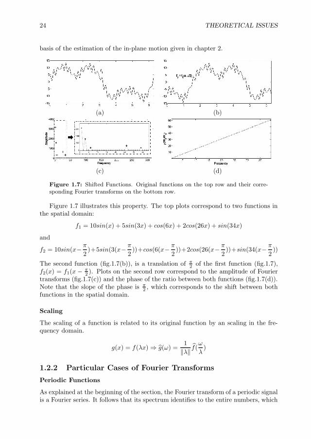
Figure 1.7: Shifted Functions. Original functions on the top row and their corre-sponding Fourier transforms on the bottom row.
Figure 1.7 illustrates this property. The top plots correspond to two functions inthe spatial domain:
f1 = 10sin(x) + 5sin(3x) + cos(6x) + 2cos(26x) + sin(34x)
and
f2 = 10sin(x− π
2)+5sin(3(x− π
2))+cos(6(x− π
2))+2cos(26(x− π
2))+sin(34(x− π
2))
The second function (fig.1.7(b)), is a translation of π2 of the first function (fig.1.7),
f2(x) = f1(x − π2 ). Plots on the second row correspond to the amplitude of Fourier
transforms (fig.1.7(c)) and the phase of the ratio between both functions (fig.1.7(d)).Note that the slope of the phase is π
2 , which corresponds to the shift between bothfunctions in the spatial domain.
Scaling
The scaling of a function is related to its original function by an scaling in the fre-quency domain.
g(x) = f(λx) ⇒ g(ω) =1
‖λ‖ f(ω
λ)
1.2.2 Particular Cases of Fourier Transforms
Periodic Functions
As explained at the beginning of the section, the Fourier transform of a periodic signalis a Fourier series. It follows that its spectrum identifies to the entire numbers, which

1.2. Fourier Transform 25
is a discrete set. On the other side, the Fourier transform of non-periodic signals hasa continuous spectrum, that is, it identifies to the real line.
(a) (b)
(c) (d)
Figure 1.8: Fourier transforms of periodic and non-periodic functions. On the toprow, the original functions, periodic (a) and non-periodic (b). On the bottom row, thecorresponding Fourier transforms for the periodic function (c) and the non-periodicone (d).
The functions in figure 1.8 illustrate this phenomenon. Top plots show the periodicfunction,
f1 = 10sin(x) + 5sin(3x) + cos(6x) + 2cos(26x) + sin(34x)
on the left (fig.1.8(a)) and the same function with a non-periodic term,
f2 = x2 + 10sin(x) + 5sin(3x) + cos(6x) + 2cos(26x) + sin(34x)
on the right (fig.1.8(b)). Bottom plots show the amplitudes (given by absolute values)of their Fourier transforms. Note that the five non-zero frequencies in the periodicfunction are reflected as 5 clear peaks in its Fourier transform. Meanwhile, the valuesof the Fourier transform of the non-periodic function cover the whole Fourier spectrumand present an exponential decay.
Smooth Functions
Regardless of its discrete nature, which is given by the function periodicity, Fourierspectra for functions infinitely differentiable (C∞) might be of compact (closed andbounded subset) support or not. Compactness is independent of the discrete nature,since there exist non-compact discrete sets (e.g. the natural numbers) as well ascompact non-discrete sets (e.g. the [0, 1] interval). In the case of a differentiablefunction of compact support, its derivatives are integrable functions. This implies

26 THEORETICAL ISSUES
(proposition 1.5.3) that the Fourier transform of the derivatives exists and satisfies:
f (k)(ω) = (2πiω)kf(ω)
Since f (k)(ω) is integrable, ‖ωk‖‖f(ω)‖ < ε for large values of ω. It follows
that ‖f(ω)‖ < ε‖ωk‖ and, since ωk is a polynomial, f ∈ L1 has to be a function of
rapid decay. In practical terms, this implies that high frequency coefficients are smallenough to be neglected. That is, low-pass filters give a good approximation of thiskind of functions.
1.3 Anisotropic Restricted Operators
By their faint and inhomogeneous appearance, in order to detect vessel layers (spe-cially adventitia), IVUS images should be filtered first. In this section, we explainthe mathematical formulation of a non-linear filtering operator able to preserve grey-level along transitions between vessel layers without altering their shape. At thesame time, if the boundary conditions are changed, the differential operator is ableto restore smooth contours consistent with vessel layers geometry.
Solutions to the heat diffusion equation with initial condition a given image,I0(x, y), provide a time (scale) dependant family, I(x, y, t), of smoothed versions ofI0(x, y). Heat diffusion is given in divergence form as:
It(x, y, t) = div(J∇I), I(x, y, 0) = I0(x, y) (1.6)
where ∇I = (Ix, Iy) is the image gradient, div is the divergence operator and J is a2-dimensional symmetric (semi-) positive defined tensor that locally describes the waygrey level re-distributes. It follows that J diagonalizes in an orthonormal basis (seesection 1.1). Heat equation is thoroughly described by means of J eigenvectors (ξ,η = ξ⊥) and eigenvalues (λ1,λ2), which describe the preferred diffusion directions ofthe heat. Symmetric semi-positive defined tensors define a metric in Euclidean space.The unitary vectors associated to the metric are an ellipse with axis of length λ1, λ2
oriented along ξ, ξ⊥. The shape of such ellipse also describes the preferred diffusionof heat. In this sense, we can talk about isotropic diffusion (equal eigenvalues) andanisotropic diffusion (distinct and strictly positive eigenvalues). By general theoryof partial differential equations [76], equation (1.6) has a unique solution providedthat λ1, λ2 do not vanish. However, in such case, I(x, y, t) converges to a constantimage [53], so that the diffusion time (iterations in numeric implementations) is acritical issue for restoring an image preserving meaningful structures (terminationproblem [77]).
In [57], it is shown that, for null eigenvalues, existence and uniqueness of solutionsto (1.6) is guaranteed as long as the eigenvector of positive eigenvalue defines a dif-ferentiable curve. In this case, J represents the projection matrix onto the positiveeigenvector and diffusion restricts to its integral curves. Depending on the boundaryconditions equation (1.6) models a smoothing process (Neumann conditions) or anextension one (Dirichlet).

1.3. Anisotropic Restricted Operators 27
1.3.1 Structure-Preserving Diffusion
The second moment matrix [78] or Structure Tensor [79] provides a good descriptionof local image structures. The Structure Tensor tensor matrix, STρ,σ describes thegradient distribution in a local neighborhood of each pixel by averaging the projectionmatrices onto the image gradient:
STρ,σ = g(ρ) ∗[(
Ix(σ)Iy(σ)
)(Ix(σ), Iy(σ))
]=
(g(ρ) ∗ I2
x(σ) g(ρ) ∗ Ix(σ)Iy(σ)g(ρ) ∗ Ix(σ)Iy(σ) g(ρ) ∗ I2
y (σ)
)
Image derivatives are computed using gaussian kernels, gσ, of variance σ (differenti-ation scale):
Ix(σ) = g(σ)x ∗ I and Iy(σ) = g(σ)y ∗ I
The projection matrix onto the image gradient, ∇I = (Ix(σ), Iy(σ)) is averaged usinga gaussian of variance ρ (integration scale). Since ST (ρ, σ) is the solution to the heatequation with initial condition the projection matrix, its eigenvectors are differentiable(smooth) vector fields that represent image level sets normal (principal eigenvector,ξ) and tangent (secondary eigenvector, ξ⊥) spaces. In the absence of corners (likeanatomical contours in bottom right image in fig.1.9), the vector ξ⊥ is oriented alongimage consistent contours (in the sense of regular differentiable curves [80]). At tex-tured or noisy regions, ξ⊥ is randomly distributed (upper right image in fig.1.9).
The Structure-Preserving Diffusion (SPD) is given by:
It = div(QΛQt∇I), I(x, y, 0) = I0(x, y) (1.7)
with:
Q =(ξ⊥, ξ
)and Λ =
(1 00 0
)
for ξ the principal eigenvector of ST (ρ, σ). By ξ⊥ distribution (fig.1.9), SPD smoothesimage grey values along regular structures (bottom right image in fig.1.9) and per-forms like a gaussian filter at textured and noisy regions (upper right image in fig.1.9).Its geometric nature makes the restricted diffusion evolution equation converge to anon trivial image that preserves the original image main features as curves of uniformgray level [57]. In this manner, SPD output achieves a uniform response to local imagedescriptors suitable for a further detection and segmentation of image (anatomical)regions.
Let us illustrate the benefits of SPD in medical imaging processing by applying itto cardiac Magnetic Resonance (MR) images of the left ventricle in short axis (SA) andlong axis (LA) views. Fig.1.10 shows grey-level images and region segmentation forLA (top rows) and SA (bottom rows) views for, from left to right, non-processed, SPD,anisotropic filtering [53] and median filtering [81]. We have segmented three regions:blood (shown in white), myocardial walls (shown in grey) and background (shownin black). In original views (left columns) magnetic noise miss-classifies some pixels(identified as background) at myocardial regions. Miss-classifications still remain inanisotropic views (third column). SPD (second column) and median (forth column)filters solve this problem, but median views over-classify them, while myocardial walls

28 THEORETICAL ISSUES
Figure 1.9: Vector field representing level curves of an angiography for a vessel(bottom-right image) and a background structure-less area (upper-right image).
maintain its shape on SPD views. Regarding blood, in original images of LA views wecan notice a thin dark line corresponding to a valve, which is detected in SPD view,almost detected in anisotropic view and suspected in median view. We can noticethe same effect in SA views for the thin dark line embedding the right ventricle (onthe left side of the images) and the trabeculae on the left ventricle, which are overdetected in anisotropic view and miss-detected in median view.
1.3.2 Anisotropic Contour Closing
If boundary conditions of equation (1.6) are changed to Dirichlet [76], the processgoverned by the equation results in a functional extension process. Such processescan be used to complete unconnected contours [58] as follows.
Let γ0 be the set of points to connect, χγ0 its characteristic function (a mask)
and J the metric defined in equation (1.7). Then, the extension process, namedAnisotropic Contour Closing (ACC):
It = div(J∇I) with I|γ0= χγ0 =
1, if the pixel belongs to γ0;0, otherwise.
(1.8)
converges to a closed model of γ. Intuitively, we are integrating the vector field ξ, thatis, we are interpolating the unconnected curve segments along it. This fact endowsACC with two main advantages over other closing techniques, such as snakes [82].First, the use of a restricted heat equation (1.8) ensures convergence to a closedmodel of the unconnected curve, whatever its concavity is. Second, because ξ takesinto account image level sets geometry, ACC closures are more accurate than otherinterpolating techniques (such as geodesic snakes [82]) which, at most, yield piece-wiselinear models.

1.3. Anisotropic Restricted Operators 29
Figure 1.10: Performance of smoothing approaches on cardiac magnetic resonanceimages.
In order to avoid wrong continuations at noisy areas, the vector ξ is weighted bythe coherence of the Structure Tensor. This quantity measures the vector regularityand is given by:
coh =(λ1 − λ2)
2
(λ1 + λ2)2
for λ1 ≥ λ2, STρ,σ eigenvalues. At regions where ξ is a continuous vector, λ2 is closeto zero, so coh is maximum, meanwhile, at noisy areas, since ξ is randomly oriented,λ1 compares to λ2 and coh ∼ 0.
The vector guiding ACC is defined by:
ξ = coh ξ (1.9)
for ξ the minimum eigenvalue of the Structure Tensor STρ,σ
Figure 1.11 illustrates the performance of ACC on an image of a human brain(fig.1.11(a)). Contours detected using a Canny edge detector are shown in fig.1.11(b).The unconnected contours which should be completed are better shown in the zoom offig.1.11(c). The mask shown in fig.1.11(d) corresponds to the characteristic function

30 THEORETICAL ISSUES
(a) (d)
(b) (e)
(c) (f)
Figure 1.11: Anisotropic Contour Closing
obtained from the extension process (equation (1.8)). Finally, in fig.1.11(e) we showthe image ridges of mask yielding the ACC closure. The close-up of figure 1.11(f)shows the completeness of contours and their agreement to the original geometry ofthe brain folds.
1.4 B-snakes
The amount of images involved in an IVUS sequence suggests searching for a contourrepresentation as compact as possible. This motivates guiding a parametric B-snaketowards ACC closure to obtain a compact smooth explicit representation.
A parametric snake is a curve γ(u) = (x(u), y(u)) which, under the influence ofan external force, Eext, and internal constrains, Eint, models a target curve γτ by

1.4. B-snakes 31
minimizing the energy functional:
E(γ) =
∫
γ
(Eint(γ) + Eext(γ, γτ ))du
=
∫
γ
(1
2α‖γ‖2 +
1
2β‖γ‖2 + Eext(γ, γτ ))du (1.10)
=
∫F (γ, γ, γ)du
The external energy, Eext, is an external potential achieving a minimum on γτ , whichfaithfully preserves the target curve. The internal energy, Eint, preserves the conti-nuity and smoothness of γ, weighted by α, β ∈ [0, 1].
The minimum of (1.10) is found by canceling the first derivative of E given by theEuler-Lagrange equation [76]:
Fγ − du(Fγ) + duu(Fγ) = 0
where du and duu correspond to the first and second derivatives, respectively, of thefunction F . This equation leads to solving the following system of 2 equations:
−αxuu + βxuuuu + ∂Eext
∂x = 0
−αyuu + βyuuuu + ∂Eext
∂y = 0
In the discrete case the curve γ is defined by a sampling of n points (x1, . . . , xn, y1, . . . , yn)so that the energy functional (1.10) converts to:
E =
n∑
i=1
Eint(i) +
n∑
i=1
Eext(i)
The corresponding Euler-Lagrange equations are a system of 2n equations which canbe written in matrix form:
Ax = −∂Eext
∂x
Ay = −∂Eext
∂y
(1.11)
where A is a penta-diagonal matrix called the stiffness matrix and expressed by:
2α + 6β −α − 4β β 0 0 0 . . . β −α − 4β−α − 4β 2α + 6β −α − 4β β 0 0 . . . 0 β
β −α − 4β 2α + 6β −α − 4β β 0 0 . . . 00 β −α − 4β 2α + 6β −α − 4β β 0 . . . 0...
......
......
......
......
−α − 4β β 0 0 . . . 0 β −α − 4β 2α + 6β
The system (1.11) is solved iteratively by writing it as:
(A + δI)x = δx − ∂Eext
∂x
(A + δI)y = δy − ∂Eext
∂y

32 THEORETICAL ISSUES
for any scalar δ. Thus we have:
x = (A + δI)−1(δx − ∂Eext
∂x )
y = (A + δI)−1(δy − ∂Eext
∂y )
So that, the iterative scheme is given by:
xt+1 = (A + δI)−1(δxt − ∂Eext
∂x )
yt+1 = (A + δI)−1(δyt − ∂Eext
∂y )
1.5 Proofs
This section is devoted to mathematically prove some assumptions about polar coor-dinates transforms and Fourier development made along the chapter.
Proposition 1.5.1 The points
(xy
)=
(cos θ − sin θsin θ cos θ
)·(
λ1 00 λ2
)·(
xy
)
of a body undergoing a rotation of angle θ followed by a dilation of factor λ = (λ1, λ2)in Cartesian coordinates, in polar coordinates corresponds to:
r =
√(λ1x)2 + (λ2y)2
α = atan(
λ2yλ1x
)+ θ
(1.12)
Proof By applying (1.12) to equations of (x′, y′) we obtain the following:
r2 = x′2 + y′2 = (λxxcosθ − λyysinθ)2 + (λxxsinθ + λyycosθ)2
= (λxx)2 + (λyy)2
So, r =√
(λxx)2 + (λyy)2
The same steps for the angle:
tan(α) =sin(α)
cos(α)=
y
x
sin(α)
cos(α)=
λxxsin(θ) + λyycos(θ)
λxxcos(θ) − λyysin(θ)
sin(α) · (λxxcos(θ) − λyysin(θ)) = cos(α) · (λxxsin(θ) + λyycos(θ))
λxx · (sin(α)cos(θ) − cos(α)sin(θ)) = λyy · (sin(α)sin(θ) + cos(α)cos(θ))
λxx · sin(α − θ) = λyy(cos(α − θ))
tan(α − θ) =λyy
λxx
So, α = atan(
λyyλxx
)+ θ

1.5. Proofs 33
Proposition 1.5.2 Let f, g ∈ L1(R) be two functions. Then, they satisfy the follow-ing properties:
1. Linearity. (λf + µg) = λf + µg
2. Convolution. f ∗ g = f · g3. Translation. g(x) = (τzf)(x) = f(x − z) ⇒ g(ω) = f(ω)e−2πiωz
4. Scaling. g(x) = f(λx) ⇒ g(ω) = 1‖λ‖ f(ω
λ )
Proof 1. (λf + µg) = λf + µg
(λf + µg)(ω) =
∫ ∞
−∞
(λf(x) + µg(x))e−2πiωxdx
= λ
∫ ∞
−∞
f(x)e−2πiωxdx + µ
∫ ∞
−∞
g(x)e−2πiωxdx
= λf + µg
2. f ∗ g = f · g
f ∗ g(x) =
∫ ∞
−∞
(f ∗ g)(x)e−2πiωxdx
=
∫ ∞
−∞
∫ ∞
−∞
f(t)g(x − t)dte−2πiωxdx
=
∫ ∞
−∞
∫ ∞
−∞
f(t)g(x − t)e−2πiωx+2πiωt−2πiωtdxdt
=
∫ ∞
−∞
∫ ∞
−∞
f(t)g(x − t)e−2πiω(x−t)e−2πiωtdxdt
=
∫ ∞
−∞
f(t)e−2πiωtdt
∫ ∞
−∞
g(y)e−2πiω(y)dy
= f · g
3. If g(x) = (τzf)(x) = f(x − z), then g(ω) = f(ω)e−2πiωz
g(ω) =
∫ ∞
−∞
g(x)e−2πiωxdx =
∫ ∞
−∞
f(x − z)e−2πiωxdx
=
∫ ∞
−∞
f(x − z)e−2πiωze−2πiω(x−z)dx = e−2πiωz
∫ ∞
−∞
f(x − z)e−2πiω(x−z)dx
= e−2πiωz f(ω)

34 THEORETICAL ISSUES
4. If g(x) = f(λx), then g(ω) = 1‖λ‖ f(ω
λ )
g(ω) =
∫ ∞
−∞
g(x)e−2πiωxdx =
∫ ∞
−∞
f(λx)e−2πiωxdx =
∫ ∞
−∞
1
λf(y)e−2πi ω
λydy
=1
‖λ‖
∫ ∞
−∞
f(y)e−2πi ωλ
ydy =1
‖λ‖ f(ω
λ
)
Proposition 1.5.3 If f, f ′, f ′′, · · · , f (k) ∈ L1(R) then, f (k)(ω) = (2πiω)kf(ω)
Proof Integrating by parts we have:
f ′(ω) =
∫ ∞
−∞
f ′(x)e−2πiωxdx =[f(x)e−2πiωx
]x→∞
x→−∞+ 2πiω
∫ ∞
−∞
f(x)e−2πiωxdx
By Cauchy theorem [80]and since f is integrable, the first term vanishes. By
induction we obtain f (k)(ω) = (2πiω)kf(ω)

Chapter 2
Physics-based Models for Vessel
Dynamics Exploring
Tissue bio-mechanical properties (like strain and stress) are playing an increasingrole in diagnosis and long-term treatment of intravascular coronary diseases. Theirassessment strongly relies on estimation of vessel wall deformation. Since IntraVascu-lar UltraSound (IVUS) sequences allow visualizing vessel morphology and reflect itsdynamics, this technique represents a useful tool for evaluation of tissue mechanicalproperties.
Image misalignment introduced by vessel-catheter motion is a major artifact fora proper tracking of tissue deformation. In the first section of this chapter, we assessIVUS rigid in-plane motion due to heart beating. Motion parameters are computedby considering both the vessel geometry and its appearance in the image. In thecase of IVUS sequences, due to its acquisition nature, different dynamic componentsare reflected in these transformations, not only cardiac component. On one hand,breathing forces a periodic displacement of arteries. On the other one, vessel geometry(curvature and torsion) influences on the relative position between catheter and artery.We decompose dynamics into geometric and motion components and identify the roleof each term.
On the other side, longitudinal motion artifacts in IVUS sequences hinders aproperly 3D reconstruction and vessel measurements. Most of current techniquesbase on the ECG signal to obtain a gated pullback without the longitudinal artifactby using a specific hardware or the ECG signal itself. The potential of IVUS imagesprocessing for phase retrieval still remains little explored. In section 2.2, we presentan image-based approach for cardiac phase retrieval from coronary IVUS sequenceswithout ECG signal. Inspired on the fact that maximum and minimum lumen areasare related to end-systole and end-diastole, our cardiac phase retrieval is based on theevolution of physical quantities along the sequence and statistically explores which isthe best filter for extracting it.
Finally, the mathematical issues supporting some assumptions made along thechapter are detailed in section 2.3.
35

36 DYNAMICS EXPLORING
2.1 In-plane Dynamics
Different factors such as heart pumping, blood pressure or artery geometric propertiesmainly contribute to the dynamics of coronary arteries [21, 71, 72]. The first orderapproximation to vessel in-plane dynamics is given by a linear transformation com-bining translation, rotation and scaling [73]. Dilation is inherent to the elasticity ofthe vessel itself and it does not preserve the metric. The rigid part of this approxi-mation can be modeled as a rigid body motion and is given by a rotation followed bya translation.
In body dynamics, the point describing the object response to external forces andtorques is determined by means of its center of gravity or mass [83]. The differencebetween its position and the origin of coordinates is identified to the object translation.In this framework, the object motion is given by a rotation centered at its center ofmass, which position is identified to the object translation. If the center of mass ofthe object at time zero is taken as origin, then the linear application mapping theobject at a given time to the object at time zero (section 1.1 of chapter 1) is given by:
(xy
)=
(cos θ − sin θsin θ cos θ
)·(
x − t1y − t2
)(2.1)
for ~t = (t1, t2) the position of the center of mass and θ the angle of rotation in radians.Rigid motion parameters are computed by combining vessel geometry and appearanceas follows.
2.1.1 Translation
Since IVUS sequences are centered at the catheter (which coincides with the centerof the image), vessel translation is given by position of the center of gravity of thevessel, namely V CM , at each frame.
Since grey level reflects tissue mass density due to IVUS images reconstruction,the center of mass given by the image intensity, namely ICM , corresponds to thephysical center of gravity of the vessel. However, some acquisition devices allow inter-active tuning of the image brightness in order to enhance tissue and vessel structuresappearance [84]. Such intensity gain is radial [85], and the image is made-up fromthis tuning. Thus, tissue close to the catheter might look brighter and, for vesselsnot centered at the catheter, intensity gainings might deviate the position of ICMfrom the true center of mass. Vessel geometric center, namely GCM , coincides withthe vessel center of gravity only in the case of uniform tissue density. However, itserves to compensate the deviation of ICM for non centered vessels. We define thecenter of mass of the vessel, V CM , by a combination of ICM and GCM achievinga good compromise between vessels whose intensity gain has been tuned and vesselswith uniform tissue density.
Image Center of Mass - ICM
Let I be an image of dimensions n × m and (i, j) be the pixel position in the image.The center of mass of the image (ICM) is given by averaging image pixel positionsweighted by their grey-value intensity:

2.1. In-plane Dynamics 37
ICM =
(∑ni=1 i
∑mj=1 I(i, j)∑n
i=1
∑mj=1 I(i, j)
,
∑mj=1 j
∑ni=1 I(i, j)∑n
i=1
∑mj=1 I(i, j)
)
Geometric Center of Mass - GCM
The geometric center (GCM) of a set of N image points, (xk, yk)1≤k≤N , is computedas the average of their positions:
GCM =1
N
(N∑
k=1
xk,
N∑
k=1
yk
)
In the case of IVUS sequences, the most reliable geometric center of the vessel isthe center of the transition between media and adventitia layers, since it is the vesselstructure which best preserves its shape, regardless of morphological changes. Thus,the points chosen to compute the geometric center are a set roughly lying on thistransition (which is named adventitia for convenience). The strategy to extract thesepoints is an iterative algorithm based on a temporal analysis along the sequence [56].
1. Lumen Displacement Reduction. In polar coordinates with the origin at thecenter of the image, the vessel appears as a straight band as far as it is centeredat the catheter. Any deviation between the vessel and the catheter results ina undulate profile. The lumen displacement along the sequence converts into adynamic radial wave. Such wave is suppressed by transforming images to polarcoordinates with origin fixed at ICM . We name Ipol such polar images.
2. Negative Edge extraction. The points roughly lying on the adventitia areextracted by means of negative horizontal edges, ey, of the polar images, Ipol.Edges are computed by convolving Ipol with the y-partial derivative of a 2dimensional gaussian kernel of variance ρ:
ey(i, j) = gy(i, j) ∗ Ipol(i, j)
for gy(i, j) = − j
2πρ4e−(i2+j2)/(2∗ρ2)
3. Geometric Displacement Reduction: The impact of noise and artifacts isminimized by considering the average of ey for a block of N sequence frames.Vessel curvature displacement produces a blurring of the energy average atcurved angular sectors. The number of frames achieving the best compromisebetween small artifacts removing and tissue blurring is approximately a third ofthe heart cycle (10 frames in pull-backs at 30 frames per second). We select foreach angle (column) those points with the former average below the 5% radialpercentile. Spurious edges due to noise and other sparse artifacts (such as bloodscatter at branches) are removed by applying a length filtering to the extractededges that leaves only those connected components of a length above a givenvalue. In order to endow further continuity to the selected segments, we use thestatistical distribution of their radial position along a block of images.
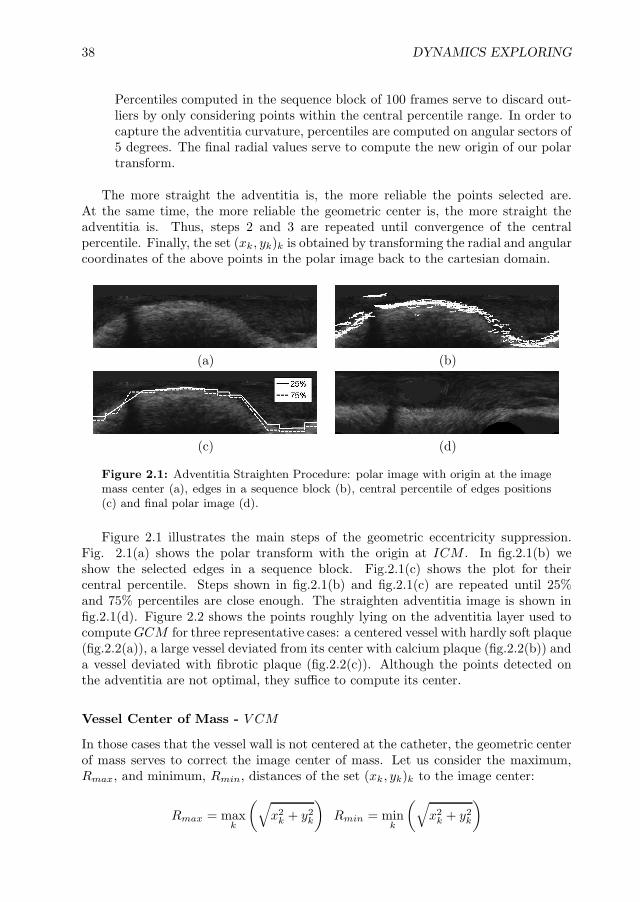
38 DYNAMICS EXPLORING
Percentiles computed in the sequence block of 100 frames serve to discard out-liers by only considering points within the central percentile range. In order tocapture the adventitia curvature, percentiles are computed on angular sectors of5 degrees. The final radial values serve to compute the new origin of our polartransform.
The more straight the adventitia is, the more reliable the points selected are.At the same time, the more reliable the geometric center is, the more straight theadventitia is. Thus, steps 2 and 3 are repeated until convergence of the centralpercentile. Finally, the set (xk , yk)k is obtained by transforming the radial and angularcoordinates of the above points in the polar image back to the cartesian domain.
(a) (b)
(c) (d)
Figure 2.1: Adventitia Straighten Procedure: polar image with origin at the imagemass center (a), edges in a sequence block (b), central percentile of edges positions(c) and final polar image (d).
Figure 2.1 illustrates the main steps of the geometric eccentricity suppression.Fig. 2.1(a) shows the polar transform with the origin at ICM . In fig.2.1(b) weshow the selected edges in a sequence block. Fig.2.1(c) shows the plot for theircentral percentile. Steps shown in fig.2.1(b) and fig.2.1(c) are repeated until 25%and 75% percentiles are close enough. The straighten adventitia image is shown infig.2.1(d). Figure 2.2 shows the points roughly lying on the adventitia layer used tocompute GCM for three representative cases: a centered vessel with hardly soft plaque(fig.2.2(a)), a large vessel deviated from its center with calcium plaque (fig.2.2(b)) anda vessel deviated with fibrotic plaque (fig.2.2(c)). Although the points detected onthe adventitia are not optimal, they suffice to compute its center.
Vessel Center of Mass - V CM
In those cases that the vessel wall is not centered at the catheter, the geometric centerof mass serves to correct the image center of mass. Let us consider the maximum,Rmax, and minimum, Rmin, distances of the set (xk , yk)k to the image center:
Rmax = maxk
(√x2
k + y2k
)Rmin = min
k
(√x2
k + y2k
)

2.1. In-plane Dynamics 39
(a) (b) (c)
Figure 2.2: Detection of points roughly lying on the adventitia for different mor-phologies with the corresponding geometric center. A centered vessel with hardlysoft plaque (a), a vessel not centered at the catheter with fibrotic plaque (b) and alarge vessel not centered at the catheter with calcium plaque (c).
and, denoted by DR, the vessel-catheter deviation rate given by:
DR =Rmin
Rmax
Then, the vessel center of mass, V CM , is defined as:
V CM = DR · ICM + (1 − DR) · GCM (2.2)
Figure 2.3 shows the three different centers of mass for a vessel not centered atthe imaging catheter. In fig.2.3(a), ICM appears nearly centered in the image, butnot centered in the vessel. In fig.2.3(b), GCM is centered in the vessel, so it correctsICM to the final V CM in fig.2.3(c).
(a) (b) (c)
Figure 2.3: Center of gravity computations: ICM (a), GCM (b) and VCM (c).

40 DYNAMICS EXPLORING
2.1.2 Rotation
Once vessel translation has been compensated, two global motions still remain: ro-tation and radial scaling. According to (subsection 1.1.1), in the polar domain withorigin V CM , they convert into a horizontal translation (corresponding to rotation)and a vertical scaling, (corresponding to radial scaling). Let I1, I2 be two consecutivepolar frames (with origin at V CM) of the sequence and let us assume an isometricdilation. By proposition 1.5.1 they are related via:
I2(i, j) = I1(i + θ, λj)
where θ corresponds to the angle of rotation and λ to the dilation.In the case of human coronary arteries, scaling is very close to 1 [86], so λ = 1 + ε
becomes a perturbation of identity given by ε. Furthermore, we restrict computationsto a band around the media-adventitia layer, given by j = j0 + ∆j. By Taylor’sformula [80], it follows that the first order approximation to I2 is given by:
I2(i, j) = I1(i + θ, j + εj) ∼ I1(i + θ, j) + εj∂jI1(i + θ, j)
= I1(i + θ, ∆j + j0) + εj∂jI1(i + θ, j)
for ∂j denoting the partial derivative with respect to the second variable.Since t and j0 are constant shifts, the first order approximation to I2 can be
computed by applying the Fourier transform [87] and using phase correlation [88].
Let I1, I2 be the Fourier transforms of I1, I2 and let us assume that they differ in apure translation:
I2(i, j) = I1(i − t1, j − t2) [= I1(i + θ, ∆j + j0)]
then their Fourier transforms are related (proposition 1.5.2) via:
I2(ω) = I1(ω)e−i〈ω,t〉
for ω = (ω1, ω2) the Fourier frequency, ~t = (t1, t2) and 〈ω,~t〉 = ω1t1 + ω2t2 theEuclidean scalar product.
If we consider the phase, ρ(ω), of the ratio between the two Fourier transforms [89],we have that:
ρ(ω) = ρ
(I2(ω)
I1(ω)
)= ρ
(e−i〈ω,t〉
)= 〈ω, t〉 = ω1t1 + ω2t2
so that the points (ω1, ω2, ρ(ω)) lie on a plane, Π, with the slopes given by the trans-lation:
Π : ρ(ω) = t1ω1 + t2ω2
In practice, noise and texture introduce a scatter in the set (ω1, ω2, ρ(ω)), es-pecially for those frequencies with smaller amplitudes. We reduce noise-scatter byonly considering those frequencies common to both images with an associated ampli-tude larger than a given percentile. Such frequencies with the phase ρ yield a point

2.1. In-plane Dynamics 41
Figure 2.4: Regression plane approximating Fourier phase correlation between twoshifted images.
cloud, like the one shown in figure 2.4, which regression plane provides a least-squareestimator of the plane Π.
The first slope of the regression plane estimates the angle of rotation between twoconsecutive frames. Since polar coordinates cover 360 degrees, rotation angles aregiven in the range [−π, π] ≡ [−180o, 180o]. This range covers all possible rotationalmotions because a rotation angle is determined modulus 2kπ radians due to such arotation does not affect the appearance of the image/structure undergoing it. Therotation of each image at time k with respect to a reference frame at time 1 is com-puted by accumulating all frame-to-frame rotation angles. That is, let θk−1,k be therotation angle between two consecutive frames at times k−1 and k, then the rotationangle aligning the k-th frame to a first one is given by:
θk :=
j=k∑
j=1
θj−1,j (2.3)
The reliability of the rotation angle is related to the regression plane fitting error(residuals). Large residuals indicate a poor linear dependency between frequency andphase. In this cases, the estimated parameter does not properly approach the rotationangle and should be discarded. Since polar images are 360 pixels wide, anomalouscases are detected by a mean fitting error over 1 (degree/pixel). Such angles constituteless than 6.43% of the data analyzed and their values are interpolated along thesequence using the preserved angles.
For a detailed explanation of the mathematical argumentations supporting theassumptions made in our estimation of the rotation angle, the reader can have a lookat section 2.3.

42 DYNAMICS EXPLORING
2.1.3 Dynamics Decomposition
The rigid motion that cardiac vessels undergo is a complex dynamical process whichresults from the combination of several contributions. In general, it presents a ge-ometric component related to the artery 3D shape and a dynamic one induced bybreathing and cardiac movements [7]. Depending on the particular problem to ap-proach, each of the terms should have specific treatment. Exploring artery geometrymight be derived by analyzing the geometric component [90], whereas extraction ofcardiac dynamics concerns the cardiac dynamical contribution [16]. In the case ofvessel biomechanics analysis, the goal is to produce a static model allowing a bettertissue tracking along the segment. Firstly, the reader should note that, without fur-ther analysis, the geometric component does not reach a reliable 3D representation ofthe vessel geometry, which might lead to wrong static models. Secondly, even if onecould infer the true 3D geometry from it, by compensating vessel tortuosity there isno guarantee of a better alignment of vessel plaque. This suggests only correcting thedynamical terms of the translation and rotation for stabilizing the sequence. In orderto allow a complete comprehension of vessel dynamics, this subsection is devoted toprovide the mathematical tools for decoupling each of the terms.
The translation and rotation parameters are functions of the time s. If the geo-metric term of a motion parameter is denoted by the subindex g , the cardiac term,induced by heart beating, is denoted by the subindex c and breathing contributionsare denoted by the subindex b, the angle and translation decompose into:
t(s) = tg(s) + tb(s) + tc(s) (2.4)
θ(s) = θg(s) + θb(s) + θc(s)
Focusing on the Fourier series of these components, breathing and cardiac termsare periodic and, thus, have a discrete Fourier spectrum, whereas geometry has abroad-band (non-discrete) spectrum [87]. As usual, Fourier transforms are indicatedby a hat ( ˆ ) over functions. Principal harmonics have been learned by supervisedclassification of the spectrum of a training set of 30 patients without apparent lesionsused in a study for assessment of myocardial perfusion in contrast angiography [91].Confidence intervals of the 95% yield the expected ranges for the principal frequencyof each of the periodic components. For breathing it is (10, 45) repetitions per minute(rpm), while for cardiac motion it is (45, 200) rpm. Each term in (2.4) is approachedas follows.
Geometric Component
Since the artery length is finite, the geometric component is a function of compactsupport and, thus, the derivatives of the geometric component are integrable func-tions. By proposition 1.5.3, fg is a function of rapid decay, so that, high frequencycoefficients are small enough to be neglected [86].
The geometric term is approximated with the low-frequency spectrum of the signal(low-pass filter [92]). Although part of the geometric component is categorized into thecardiac and breathing components, the range 1-10 rpm has (experimentally) provedto be a good approximation. Thus, the geometric term is enclosed by frequenciesbetween 1 and 10 rpm.

2.1. In-plane Dynamics 43
Breathing Component
The study reported in [91] indicates that, in spite of being periodic, breathing canbe defined by the whole spectrum in the interval (10,45) rpm. The ranges reportedin [91] were obtained from a study on patients without apparent lesions performed inour laboratory for assessment of myocardial perfusion in contrast angiography [91].The frequency range was learned by supervised classification of the spectrum of atraining set of 30 patients. For each patient three different sequences were recorded:
• A sequence without contrast injection and the patient normally breathing inorder to learn diaphragm movements and background noise
• A sequence with contrast injection and the patient holding breathing for learningthe frequency range of heart beating and myocardial staining.
• A test sequence with contrast injection and the patient normally breathing.
The values of the local mean for all sequence frames provides each pixel witha function, namely LM, that describes the average contrast absorbed by the tissuealong time. Such signal is the contribution of four main phenomena: breathing, heartbeating, myocardial dyeing and noise. The amplitudes of the spectrum of the LMpatterns define a probability density function (pdf) in the frequency domain, whichwe modeled with a mixture of Gaussians [93]. The Bayes classifier for the four classesgave the frequency ranges for the physiological phenomena reported in the article.We note that ranges coincide with clinical evidence: a living human does not breathmore than 45 times per minute and its heart does not beat more than 200 times perminute.
Cardiac Component
Finally, cardiac motion principal harmonic, ωc, is defined as the first local maximumin Iωc
= (45, 200) rpm and the term is approximated by the first 10 harmonics,(kωc)k=1:10. For the sake of an efficient algorithm, ωc is approximated by the globalmaximum of Fourier transform amplitude for frequencies in the range Iωc.
It follows that the motion terms of a sequence lasting NSec seconds are given by:
tg(s) =1
T
∫
Ig
t(ω)eiωsdω θg(s) =1
T
∫
Ig
θ(ω)eiωsdω
tb(s) =1
T
∫
Ib
t(ω)eiωsdω θb(s) =1
T
∫
Ib
θ(ω)eiωsdω (2.5)
tc(s) =1
T
k=10∑
k=1
t(kωc)eikωcs θc(s) =
1
T
k=10∑
k=1
θ(kωc)eikωcs
where the period T = NSec/60 is the sequence length (in minutes) and defines thedomains of integration as Ig = (−10T, 10T ) and Ib = (−45T,−10T )∪ (10T, 45T ).
Since, even in healthy cases, the heart rate varies along the pullback, the peaksin the Fourier series are spread around the theoretic harmonic frequencies. The more

44 DYNAMICS EXPLORING
irregularities in periodicity are, the more spread around the theoretic harmonic theFourier development is. The harmonics less corrupted by noise are obtained by opticalfiltering [94]. The technique, widely used in electron crystallography, selects Fourierpeaks by thresholding the difference between the amplitude achieved at the harmonicand an average of neighboring amplitudes. Harmonics selected by optical filtering arethe only contributions to the sums in (2.5).
Figure 2.5: Motion Decomposition. Rotation angle and its Fourier decompositionon the left; geometric, breathing and cardiac terms on the right.
Figure 2.5 shows the Fourier terms decoupling for the rotation angle in the top leftplot. Vertical lines in the Fourier spectrum of the signal (bottom left plot) indicatethe ranges defined for the 3 phenomena. Dots mark the 10 cardiac harmonics andsquares the ones selected after optical filtering. The 3 components of the angle areshown in right plots.
2.2 Longitudinal Dynamics
The first step for modeling longitudinal motion in IVUS sequences is retrieving cardiacphase information. Following the general scheme shown in figure 2.6, our image-basedalgorithm to approach ECG sampling splits in three steps:
1. Extraction of Signal Reflecting Cardiac Motion: By the physical coupling[21], luminal area evolution is synchronized to other vessel cardiac phenomena,

2.2. Longitudinal Dynamics 45
Figure 2.6: Pipeline for Image-based Cardiac Phase Retrieval
such as tissue motion or rigid motion. We propose using the latter two toretrieve a signal reflecting motion.
(a) Tissue Motion: Due to the ultrasound properties, image intensity reflectsthe density of mass and, thus, changes along the sequence either comefrom morphological changes or contain information about cardiac phase.The evolution of the image Local Mean (LM) for each pixel along thesequence is a 1-dimensional signal, which profile is a combination of themorpho-geometric arterial changes and the periodic variation due to heartbeat. Vessel motion is not reflected in the whole vessel section, but onlyat some salient areas such as plaque or vessel walls. In order to minimizethe impact of these image areas we only analyze LM from those pixelsreflecting motion by an optical filtering on LM which selects them.
(b) Rigid Motion: Since rigid in-plane motion comes from artery motion dueto heart pumping, the rotation motion profile (θ) computed in section 2.1also gives information about the cardiac phase.
2. Signal Filtering for Cardiac Profile Extraction: In general, the signals re-flecting cardiac motion are a combination of morpho-geometric arterial changesand arterial dynamics (including heart beat and breathing). Furthermore, car-diac phase is not constant along the sequence. This suggests that the profilereflecting cardiac motion should be filtered. Following the literature, we use aband-pass filter in order to control the regularity of the signal.
3. Cardiac Phase Retrieval: Minimums and maximums of the filtered signalsretrieve cardiac phase at end-systole and diastole.
The extraction of the cardiac frequency, ωc, is necessary for the first two steps.We define ωc like in the subsection 2.1.3 [91], as the most prominent local maximumin the interval Iωc = (45, 200) repetitions per minute of the Fourier developmentof either LM or θ. In the case of LM signals, this process provides a ωc for eachimage pixel and the average of all ωc for a uniform sample of pixels constitutes ourapproximation to cardiac frequency.
2.2.1 Step 1 - Extraction of Signal Reflecting Cardiac Motion
1. Tissue Motion
We compute LM in sliding windows of size (empirically set) 9×9 pixels. Since cardiac
motion is a periodic signal, LM for those pixels reflecting motion should be as closeto a discrete series (given by ωc multiples) as possible. Other dynamic phenomena,
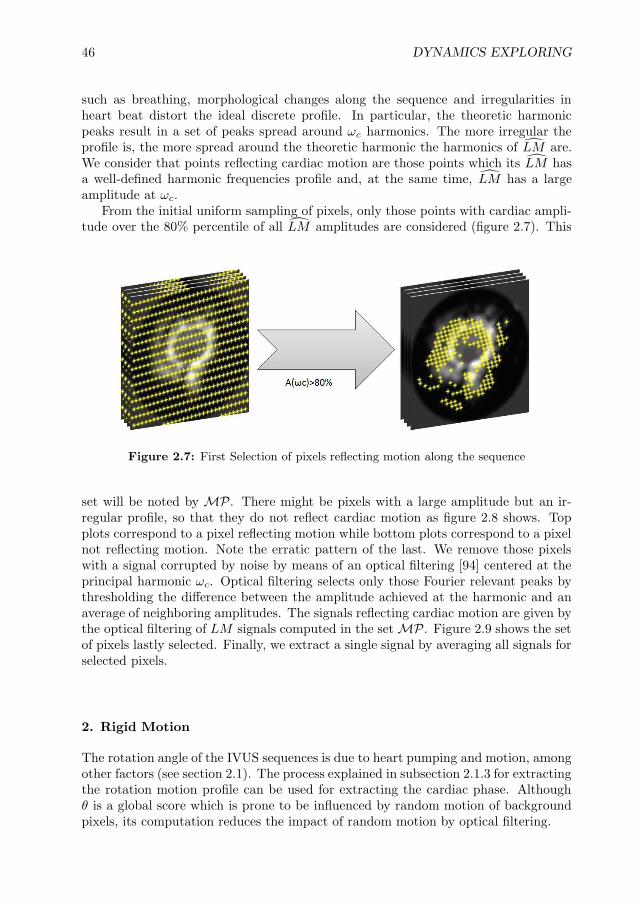
46 DYNAMICS EXPLORING
such as breathing, morphological changes along the sequence and irregularities inheart beat distort the ideal discrete profile. In particular, the theoretic harmonicpeaks result in a set of peaks spread around ωc harmonics. The more irregular theprofile is, the more spread around the theoretic harmonic the harmonics of LM are.We consider that points reflecting cardiac motion are those points which its LM hasa well-defined harmonic frequencies profile and, at the same time, LM has a largeamplitude at ωc.
From the initial uniform sampling of pixels, only those points with cardiac ampli-tude over the 80% percentile of all LM amplitudes are considered (figure 2.7). This
Figure 2.7: First Selection of pixels reflecting motion along the sequence
set will be noted by MP. There might be pixels with a large amplitude but an ir-regular profile, so that they do not reflect cardiac motion as figure 2.8 shows. Topplots correspond to a pixel reflecting motion while bottom plots correspond to a pixelnot reflecting motion. Note the erratic pattern of the last. We remove those pixelswith a signal corrupted by noise by means of an optical filtering [94] centered at theprincipal harmonic ωc. Optical filtering selects only those Fourier relevant peaks bythresholding the difference between the amplitude achieved at the harmonic and anaverage of neighboring amplitudes. The signals reflecting cardiac motion are given bythe optical filtering of LM signals computed in the set MP. Figure 2.9 shows the setof pixels lastly selected. Finally, we extract a single signal by averaging all signals forselected pixels.
2. Rigid Motion
The rotation angle of the IVUS sequences is due to heart pumping and motion, amongother factors (see section 2.1). The process explained in subsection 2.1.3 for extractingthe rotation motion profile can be used for extracting the cardiac phase. Althoughθ is a global score which is prone to be influenced by random motion of backgroundpixels, its computation reduces the impact of random motion by optical filtering.

2.2. Longitudinal Dynamics 47
Figure 2.8: Regular Profile (on top) versus irregular profile (on bottom)
Figure 2.9: Final selection of points reflecting cardiac motion
2.2.2 Step 2 - Signal Filtering for Cardiac Profile Extraction
Even in healthy subjects, cardiac frequency does not keep constant along the sequence,which introduces (among other phenomena) irregularities in the Fourier transform ofthe cardiac motion profile. Such irregularities corrupt the location of local extremaand, thus, the signal reflecting motion should be filtered. We model the extractionof cardiac phase by filtering the cardiac profile with a bandpass filter. We use twofamilies of filters: Butterworth (B) [16] and Gaussian-based (g) [17]. Both of themare centered at the cardiac frequency ωc.
The Butterworth filter is defined as follows:

48 DYNAMICS EXPLORING
B(ω) =1√
1 +(
|ω|−ωc
0.6∆ωc
)2n
where n is related to the filter decay and ∆ω = δωc to its support. Figure 2.10 shows
Figure 2.10: Butterworth filters for different parameters
Butterworth filters centered at ωc = 76.5 rep/min for four different parameters set,P1 = n = 1; δ = 0.001 in blue, P2 = n = 4; δ = 0.1 in green, P3 = n = 2; δ = 0.1in lilac, and P4 = n = 1; δ = 0.1 in red. The last three filters have equal supportwith δ = 0.1 (including low frequencies) but decreasing decays. P4 has the lessdecay, so, low frequencies of the signal would remain. P3 reduces the impact of lowfrequencies and P2 almost suppress them. Concerning P1, although it has equal decaythan P4, it is the most located around ωc as δ is the lowest one.
The Gaussian filter is defined as follows:
Figure 2.11: Gaussian filters for different parameters
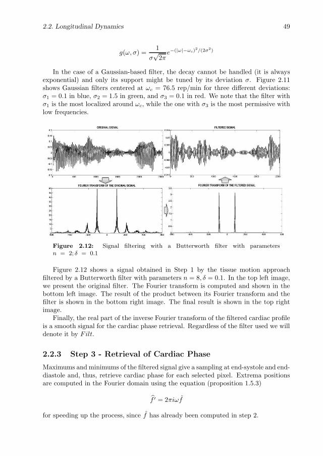
2.2. Longitudinal Dynamics 49
g(ω, σ) =1
σ√
2πe−(|ω|−ωc)
2/(2σ2)
In the case of a Gaussian-based filter, the decay cannot be handled (it is alwaysexponential) and only its support might be tuned by its deviation σ. Figure 2.11shows Gaussian filters centered at ωc = 76.5 rep/min for three different deviations:σ1 = 0.1 in blue, σ2 = 1.5 in green, and σ3 = 0.1 in red. We note that the filter withσ1 is the most localized around ωc, while the one with σ3 is the most permissive withlow frequencies.
Figure 2.12: Signal filtering with a Butterworth filter with parametersn = 2; δ = 0.1
Figure 2.12 shows a signal obtained in Step 1 by the tissue motion approachfiltered by a Butterworth filter with parameters n = 8, δ = 0.1. In the top left image,we present the original filter. The Fourier transform is computed and shown in thebottom left image. The result of the product between its Fourier transform and thefilter is shown in the bottom right image. The final result is shown in the top rightimage.
Finally, the real part of the inverse Fourier transform of the filtered cardiac profileis a smooth signal for the cardiac phase retrieval. Regardless of the filter used we willdenote it by Filt.
2.2.3 Step 3 - Retrieval of Cardiac Phase
Maximums and minimums of the filtered signal give a sampling at end-systole and end-diastole and, thus, retrieve cardiac phase for each selected pixel. Extrema positionsare computed in the Fourier domain using the equation (proposition 1.5.3)
f ′ = 2πiωf
for speeding up the process, since f has already been computed in step 2.

50 DYNAMICS EXPLORING
2.3 Mathematical Issues
As we explained in section 2.1, in the polar domain with origin CM , the remainingaffine transformations (rotation and scaling) convert into a horizontal translation(rotation) and a vertical scaling (scaling). In general, the latter would invalidateany computation of the angular translation by means of Fourier analysis and linearregression. In this section we detail the mathematical arguments that support theassumptions made in section 2.1.
In the case of human coronary arteries, scaling is very close to 1 [86], so λ = 1 + εbecomes a perturbation of identity given by ε. Furthermore, we restrict computationsto a band around the media-adventitia layer, given by j = j0 + ∆j. By Taylor’sformula, it follows that the first order approximation to I2 is given by:
I2(i, j) = I1(i+t, j+εj) = I1(i+t, j)+εj∂jI1(i+t, j) = I1(i+t, ∆j+j0)+εj∂jI1(i+t, j)
for ∂j denoting the partial derivative with respect to the second variable. Since t andj0 are constant shifts, it follows that the first order approximation is a perturbationof a pure translation which can be written as:
I2 = I1(i + t1, j + t2) + εj∂jI1(i + t, j) (2.6)
for t1 = t, t2 = j0 and the second independent variable j = ∆j. We claim that(2.6) only introduces a small (negligible) perturbation in the point cloud generatedby (ω1, ω2, ρ(ω)) not dropping regression accuracy. If we consider the ratio betweenthe Fourier transforms of I1 and I2, we have that:
I2
I1
= ei〈ω,t〉 + εj∂jI1
I1
and that the phase ρ is given by:
ρ
(I2
I1
)= Imag
log
(ei〈ω,t〉 + ε
j∂jI1
I1
)
for Imag· denoting the imaginary part of a complex number and log the com-plex logarithm. Developing again by Taylor, the first order approach to the abovelogarithm in a neighborhood of ε = 0 is given by:
log
(ei〈ω,t〉 + ε
j∂jI1
I1
)= log(ei〈ω,t〉) + εe−i〈ω,t〉 j∂jI1
I1
= i〈ω, t〉 + εe−i〈ω,t〉 j∂jI1
I1
Therefore, the points (ω1, ω2, ρ(ω)) lye on a plane perturbed by:
ρ(ω) = t1ω1 + t2ω2 + εImag
e−i〈ω,t〉 j∂jI1
I1
Figure 2.13 illustrates the impact of the perturbation, ε, in the shape of the pointcloud given by (ω1, ω2, ρ(ω)) and the coefficients of the regression plane (reported

2.3. Mathematical Issues 51
in the top boxes). We show the point cloud in the case of a pure rotation (givenby θ = 12) without scaling and the point cloud perturbed by a scaling equal to1 + ε = 1.01 (central plots) and 1 + ε = 1.045 (bottom plots). The non-perturbedpoint clouds are in circles, while the perturbed ones are in crosses. Two differentmorphologies have been considered (see images in most top row): a calcified segment(left) and a soft plaque one (right). We observe that the impact of a perturbation εis either negligible (in the sense that accuracy in regression coefficients is small) asshown in figure 2.13 (central plots) or it results in a random regression plane (fig.2.13 (bottom plots)).
Figure 2.13: Comparison between point clouds given by (ω1, ω2, ρ(ω)) in the caseof a pure rotation (circles) and a rotation perturbed by a scaling (crosses) for twodifferent morphologies, calcium (left) and soft plaque (right). The perturbation onthe central plots is ε = 0.01 while ε = 0.045 corresponds to the perturbation on thebottom plots.

52 DYNAMICS EXPLORING
The dependency between perturbation and error in translation (first slope of re-gression plane) is illustrated in the plot in figure 2.14, which shows the error of per-turbations for the image shown in the top of the first column of figure 2.13. We notethat, in this case, ε = 0.025 (dotted vertical line) is the bound for sub-pixel accuracy(left close-up) in angular translation error and perturbations above ε = 0.025 return arandom regression plane with an arbitrary error in the estimated angular translation.
Figure 2.14: Relation between perturbation and error in translation.
We claim that for human coronary arteries, the scaling between two consecutiveframes of sequences acquired at 30 fps (which is our digitalization rate) does not reachthe critical perturbation of identity. That is, let rsys and rdias denote the arterial radiiat end systole and diastole, respectively. Assuming a uniform radial scaling (given byλ) along the cycle, we have that:
rsys = λNFrrdias (2.7)
for NFr the number of frames per systolic cycle. In devices at 30 frames/sec., theaverage cardiac cycle length in adults is about 24 frames (75 beats per minute). Sincesystole approximately constitutes 40% of the cardiac cycle [95], we have that:
rsys ≈ λ10rdias (2.8)
Radial deformation of cardiac arteries mainly depends on blood pressure and vesselwall elastic properties. By Hooke’s law, the radial increment, ∆r, is proportional tothe gradient of blood pressure, ∇P , via the relation [21,71]:
∆r = (κ∇P/π)1/2
where κ is the elasticity coefficient of the coronary artery. Standard values κ =(0.010±0.020)mm/mmHg and ∇P ≈ 40 mmHg yield that the systole-diastole radialincrement is ∆r ≈ 0.35 mm [96]. Taking into account that the radii of coronarysegments [97] are in the range r = 2.64± 0.3 mm, we have that, in average, equation(2.3) equals:
rsys = rdias + ∆r ≈ 2.64 + 0.35 = 2.99 ≈ λ102.64

2.3. Mathematical Issues 53
which gives an average scaling between consecutive frames of λ = 1.0125, and, thus,a perturbation ε = 0.0125.
We have computed the error in translation for ε = 0.0125 in a set of images rep-resentative of the different vessel morphologies extracted from in vivo pullbacks. Thecorresponding error range is 1.09±0.67. We conclude that, in most cases, the pertur-bation induced by artery radial scaling does not significantly affect the computationof the angular rotation.

54 DYNAMICS EXPLORING

Chapter 3
Deterministic-Statistical Strategies
for Structures Exploring
Vessel plaque assessment by analysis of IntraVascular UltraSound sequences is a use-ful tool for cardiac disease diagnosis and intervention. Manual detection of luminal(inner) and medial-adventitial (external) vessel borders is the main activity of physi-cians in the process of lumen narrowing (plaque) quantification. Difficult definitionof vessel border descriptors, as well as, shades, artifacts, and blurred signal responsedue to ultrasound physical properties trouble automated adventitia segmentation. Inorder to efficiently approach such a complex problem, in this chapter we propose com-bining deterministic tools and statistical classification techniques into a vessel bordermodeling strategy. By the challenge of the problem, we focus on the detection of themedial-adventitial border.
3.1 General Strategy
The strategy for media-adventitia (simply adventitia from now on) segmentation wesuggest summarizes in the following three main steps:
STEP I - IMAGE PREPROCESSING
The preprocessing step splits into :
A. Polar Transformation of IVUS images
Advanced techniques for medical imaging segmentation [98] use a priori knowl-edge of the target structure shape. Active shape contours [99] are the usual wayto incorporate such knowledge to the model. In the case of the adventitia bor-der, its circular appearance can be imposed by simply transforming images topolar coordinates with the origin at the geometric center of the vessel border. Inthis coordinate system, the adventitia transforms into a horizontal curve, whichsignificantly simplifies border feature extraction.
55

56 STRUCTURES EXPLORING
B. Image Filtering IVUS images are particularly noisy, as well as, in most ofcases, adventitia appears as a very weak contour. In order to enhance significantstructures while removing noise and textured tissue, it is necessary filtering. Wepropose two different approaches.
1. Structure-Preserving Diffusion (SPD)
This diffusion [57], detailed in subsection 1.3.1, modifies classic anisotropicones [53, 100] by suppressing any diffusion across image level curves. Theassociated image operator homogenizes image structures grey values ac-cording to their geometric continuity and, thus, results in a more uniformresponse to image local descriptors (edges, valleys, ridges).
2. Sequence Stabilization
After rigid motion compensation (see section 2.1), image pixel intensity,which is related to tissue density of mass, remains more uniform alongframes. It follows that the mean of stabilized sequence blocks enhancesvessel structures, while blurring texture and speckle.
STEP II - STATISTICAL SELECTION OF BORDER POINTS
The goal of our classification stage is to compute two binary images (masks), one forvessel borders segments and another for calcium sectors. Extracting vessel bordersand calcium points requires defining the functions that best characterize each set, aswell as, their most discriminating values. We learn, both, feature space and parametricthreshold values by applying supervised classification techniques to a training set ofmanually segmented images.
A. Feature Space Design
Our feature space is designed to discriminate among the set adventitia/intima,calcium and fibrous tissue. Calcium discrimination is needed to discard angularsectors of ambiguous information and fibrous tissue to avoid miss detections ofvessel borders. By the polar coordinate system chosen, horizontal edges are themain descriptors of the set adventitia/intima. Image simple statistics (standarddeviation and cumulative means) serve to formulate the functions characterizingcalcium and fibrous plaque.
B. Extraction Parameters
In a segmentation procedure there are two kind of parameters, those that bestdiscriminate among different structures in the feature space and those actingas a filter of fake responses. Discriminating parameters are values acting asa threshold on the feature space, while filtering parameters remove spuriousdetections from the extracted segments. Both parameters are chosen and tunedto yield an optimal segmentation for a training set of manually traced borders.
STEP III - SEGMENTATION STAGE
The selection stage produces two binary images: adventitia/intima points and cal-cium sectors. Vessel border segments are modeled by computing an implicit closedrepresentation and, then, an explicit snake representation using B-splines.

3.2. Step 1 - Image Preprocessing 57
A. Implicit Anisotropic Contour Closing (ACC)
For the implicit closing we suggest using an Anisotropic Contour Closing [58]based on functional extension principles to complete curve segments in the im-age mask domain. The use of restricted diffusion operators enables to takeinto account image geometry and discard calcium and side branches sectors.Since ACC interpolates line segments along image level curves, the implicitreconstruction provides with a faithful closed model of vessel borders. We en-dow 3-dimensional continuity to such implicit reconstruction by topological areaconsiderations.
B. Explicit B-Snakes Representation
We define vessel contours at branching and calcified segments by interpolatingACC radial values in the polar domain with a B-spline snake. B-snakes yielda smooth representation encoded with N control points and conforming to thecompletion mechanisms of human vision [101]. In the cartesian domain thefinal smooth model yields an elliptical shape at sectors where no information isavailable.
3.2 Step 1 - Image Preprocessing
3.2.1 Polar Coordinates
In an IVUS plane, the media-adventitia border is an elliptic-like shape with a relativelysmall eccentricity (fig. 3.1(a)). In polar coordinates with the origin at the geometriccenter of the vessel, the adventitia converts into a nearly horizontal line that canbe parameterized by the radius. The geometric center does not coincide with the
(a) (b)
Figure 3.1: Adventitia images in cartesian (a) and polar coordinates (b).
ultrasound probe (image center) and has to be computed. Its computation it iswidely explained in chapter 2 and can be split in three main steps:
1. Lumen displacement reduction: In polar coordinates, adventitia is a straightline in the measure that the origin of coordinates is placed at its geometric cen-ter (figure 3.2). Any deviation from its geometric center results in an undulation

58 STRUCTURES EXPLORING
in its pattern. One source of deviation is lumen displacement due to heart dy-namics. The impact of lumen displacement is reduced by taking as origin theimage center of mass ICM .
2. Negative edges extraction: Negative horizontal edges provide points roughlylying on the adventitia. The geometric center of these points approximates thevessel geometric center.
3. Geometric displacement reduction: Displacement due to vessel curvatureis reduced by transforming images to polar coordinates with origin the newgeometric center computed in step 2.
Steps 2 and 3 are repeated until convergence.
Figure 3.2: Scheme of the strategy for approaching the geometric center of mass
Figure 3.2 shows the three main steps for extracting the points roughly lying onthe media-adventitia layer (upper side of the image) and the final result of the imagein polar coordinates with the geometric center of mass as origin. For an exhaustiveexplanation see chapter 2.
From now on, we will work with images in polar coordinates. We will noteAdvPol(i, j) the discrete polar transform of an IVUS frame, for the radius, i, andthe angle, j, given by:
i = 1, . . . , min(Nc, Nr) and j = 1, . . . , 360
where Nc, Nr are the dimensions (columns and rows) of the original IVUS image.
3.2.2 Image Filtering
1. Structure-Preserving Diffusion
We apply the Structure-Preserving Diffusion (SPD) described in subsection 1.3.1with smoothing parameters set to (σ, ρ) = (0.5, 2). One drawback of SPDsmoothing is the computational cost since it is an iterative process. In orderto increase its computational efficiency, SPD is applied in a band of interestcontaining the adventitia layer. This strategy reduces 50% the computationtime. The band is automatically defined by the minimum and maximum of thecentral percentile of pixels used for computing the geometric center. Figure 3.3

3.3. Step 2 - Statistical Selection of Border Points 59
shows an original IVUS image in polar coordinates (fig.3.3(a)), the same imagefiltered in a band by SPD (fig.3.3(a)) and its Sobel edges (fig.3.3(c)).
(a)
(b)
(c)
Figure 3.3: Image SPD Filtering. Polar transformation (a), the SPD image (b) andedges computed by Sobel detector (c)
2. Sequence Stabilization The method explained in section 2.1 has the potentialclinical application of tracking continuous vessel structures, such as vessel walls.Stabilized sequences preserve the local density of mass of structures along timein the measure that morphology remains unchanged along the sequence. Itfollows that the mean of a small number of frames enhances structures, andblurs texture and speckle. In order to achieve a good compromise betweenmorphologic changes and a minimum of frames for blurring non-structure areas,we take blocks of 10 frames. Although the result of this filtering process isless accurate than the one given by SPD, the computational cost of SPD issignificantly lower than SPD filtering. Figure 3.4 shows an image filtered bycomputing the mean over 10 frames (fig.3.4(a)) and its Sobel edges (fig.3.4(b)).
Note that Sobel edges shown in figures 3.3 and 3.4 give continuous profiles of theadventitia for both image filtering methods.
3.3 Step 2 - Statistical Selection of Border Points
The inner and outer vessel borders appearance is so similar that they are assumedto constitute a single class in the training process. Their distinct radial position

60 STRUCTURES EXPLORING
(a)
(b)
Figure 3.4: Stabilized Sequence Filtering. Image filtered by the mean of a block ofstabilized sequences (a), and edges computed by Sobel detector (b)
suffices to discriminate them [50] in the absence of echo opaque structures, such ascalcium. In such cases, the adventitia does not appear and the detection is misledtowards the intima. Since the best solution is to discard echo opaque sectors, thetraining stage also addresses their characterization. We also include fibrous tissuediscrimination because it is a main artifact confusing with the adventitia that forcesthe use of longitudinal cuts [50]. For the sake of simplicity, echo opaque structureswill often be referred to as calcium.
3.3.1 Feature Space Design
Based on visual perception, we mainly distinguish adventitia/intima by horizontaledges and echo opaque structures by their shadow underneath. Let AdvPol and (i, j)be the image in polar coordinates and their pixel position respectively. The featurespace we propose is a three dimensional space tuned to describe the adventitia/intimaset and echo opaque structures.
1. Horizontal Edges
Since in the coordinate system chosen, the adventitia layer is a horizontal darkline, horizontal edges constitute our main descriptor (see chapter 2 for theirdefinition).
The only image structures yielding large values for ey are intima, adventitia,calcium and fibrous tissue. Intima and adventitia correspond to negative values,while calcium and fibrous structures yield a negative and a positive response,one for each of their bordering sides.
The descriptors we have chosen to detect echo opaque plaques and fibrous tissue

3.3. Step 2 - Statistical Selection of Border Points 61
are their outstanding brightness and, for calcium, the dark shadow underneath.We propose the following particular functions to quantify such features.
2. Radial Standard Deviation
Striking brightness corresponds to an outlier of the pixel grey value in the radialdistribution. We measure it by means of the difference between the pixel grayvalue and the radial mean. For each pixel (i, j), we define it as
σ(i, j) = (AdvPol(i, j) − ν(θ))2
where ν(θ)) is the radial (i.e. column-wise) mean of the polar image:
ν(θ) =1
Rmax
Rmax∑
i=1
AdvPol(i, θ)
The magnitude of σ is maximum at bright structures (calcium and fibrousplaque) and minimum near the adventitia. In order to distinguish betweencalcium and fibrous plaque, we add the following shadows detector:
3. Cumulative Radial Mean
For each angle j consider the following cumulative mean:
CSj(i) =
∑n=in=Rmax
AdvPol(n, j)
Rmax − i
For angles with calcium, the function CSj(i) presents a step-wise profile incontrast to a more uniform response in the presence of fibrous plaque. It followsthat the total energy:
ecs(j) =
i=Rmax∑
i=1
CSj(i)
achieves its minimum values only at angles with calcium.
The feature space achieving a maximum separability for our training set is givenby:
(X, Y, Z) = (ey, sign(ey)√|eyσ|, ecs) (3.1)
Figure 3.5 shows the feature space for a calcified (1st column) and normal (2ndcolumn) cross-sections. The original images are in the first row, energy from thefirst derivative in vertical direction in the second row, Radial Standard Deviationin the third and Cumulative Radial mean in the fourth row. From ey energy im-ages (fig.3.5(b),(f)) we extract negative horizontal edges. Radial Standard Deviation(fig.3.5(c),(g)) shows a maximum in calcium sectors (fig.3.5(c)),and fibrous plaques

62 STRUCTURES EXPLORING
(a) (e)
(b) (f)
(c) (g)
(d) (h)
Figure 3.5: Image descriptors. Original images (a),(e) and Vessel Structures De-scriptors: Horizontal Edges (b),(f), Radial Standard Deviation (c),(g) and Cumula-tive Radial Mean (d),(h).
(fig.3.5(g)) and finally, Cumulative Radial Mean (fig.3.5(d),(h)) shows a minimumin calcium sectors (last columns in fig.3.5(d)) and angles with lack of information(middle columns in fig.3.5(h)).
3.3.2 Statistical Parameter Setting
For the computation of the vessel borders and calcium binary images, the classificationproblem we must face is discriminating among 4 different sets: adventitia/intima(Adv), calcium (Cal), fibrous structures (Fbr) and the rest of pixels (RP). Instead ofaddressing the 4-class problem as a whole, we will solve several 2-class problems in 2dimensions.
For its simplicity and proven efficient performance, Fisher linear discriminant anal-ysis [93] serves to reduce dimensionality of the feature spaces. Linear DiscriminantAnalysis searches for the linear subspace, W , that achieves a maximum separabilityamong the projected classes. In the case of Fisher, separability is measured in terms ofmaximum separation between class means and minimum within-class scatter. Mathe-matically, this criterion is formulated in terms of the ratio between the between-class,

3.3. Step 2 - Statistical Selection of Border Points 63
SB , and the within-class, SW , scatter matrices:
SB =∑c
i=1(µi − µ)(µi − µ)t
SW =∑c
i=1
∑Ni
j=1(Yj − µi)(Yj − µi)t
for c the number of classes, Ni the samples per class, µi the mean vector of each ofthem and µ the mean of all samples (Yj). Fisher discriminant criterion reduces tofinding the subspace, W , maximizing:
J(W) =|WtSBW||WtSW W|
Because SB encodes the projection onto the linear subspace given by µ1, . . . , µc, it has,at most, rank c− 1, which bounds W dimension by dim W ≤ c− 1. In the particularcase of a 2-class problem in 2 dimensions, Fisher space is a straight line (solid linein fig.3.6(a)) and discrimination between the two classes is achieved by a thresholdon the projection space (line labeled τPF1 in fig.3.6(b)), which induces a splitting ofthe feature space in two half planes. We will use a Bayesian approach [93] to selectthresholding values in terms of miss classification errors. In the two class problem, theclassic Bayesian strategy searches for the value that achieves a suitable compromisebetween the percentage of false positives and false negatives. The approach selectsa threshold in terms of how many true positives are detected without consideringthe amount of noise introduced in the positive detections. Although the criterionis widely used in classification problems, in the case of severe unbalanced classes orobject segmentation [102] it is more efficient to select thresholds in terms of the trade-off between precision and recall. Precision is defined as the data retrieved and relevantover all the data retrieved, while recall is the data retrieved and relevant over all thedata relevant as the following formulas show:
PRECISION =|TP |
|TP + FP | RECALL =|TP |
|TP + FN |In probabilistic terms, precision is the probability that an object is relevant, given
that it is retrieved, that is, an estimate of the conditional probability P (C1|R). Recallcorresponds to the probability that a relevant object is retrieved, that is, an estimateof the conditional probability P (R|C1). Following the usual set-up in informationretrieval, we define a decision rule in terms of our given observation vector X , todetermine which data is classified as C1 (the acceptance criterion). In this case thecost function is the following:
α1P1(FN) + α2P2(FP )
This is the strategy we propose for the computation of the Adv and Cal maskimages.
A. Vessel Borders Mask
Borders extraction is achieved by addressing 2 classification issues: discriminateC1=(Adv,RP) and C2=(Cal, Fbr) in the (X, Y ) plane and, then, separate Adv fromRP using X values.

64 STRUCTURES EXPLORING
τPF1
(a) (b)
Figure 3.6: Adventitia/Intima vs Calcium/Fibrous Tissue sets Discrimination. Fea-ture Space (a) and discrimination on the Fisher Projection Line (b)
We remind that Adv, Cal and Fbr are the only tissues yielding large responsefor X values. It follows that the clustering proposed (C1, C2) ensures that afterdiscriminating between Adv and RP, the set classified as Adv will not include anyother structures but vessel borders. This avoids the use of longitudinal cuts [50] todistinguish between intima and adventitia, since they are directly identified by theirradius.
We discriminate C1 (positives) and C2 (negatives) by projecting onto the Fisherspace, PF1, (see fig.3.6(a)). Since our discriminating problem is detecting as muchpoints on the adventitia as possible, we tune the standard Bayesian threshold in orderto achieve a maximum number of true C1 detections regardless of false positives (seefig.3.6(b)). Such miss classifications are discarded in the subsequent discriminatingand filtering steps. Among all thresholds ensuring at least 90% of true C1 detections,we choose the value, τPF1, that, in combination with the rest of parameters, yieldsoptimal segmentation results. Figure 3.6 summarizes the main steps of the discrim-ination between C1 and C2. Figure 3.6(a) shows the feature space chosen and theFisher projection line. Figure 3.6(b) the projected classes onto PF1 and a thresholddiscriminating line τPF1.
Discrimination between Adv and RP is achieved in the X coordinate domain, asAdv corresponds to large negative values. Large range of Adv values among differentpatients, suggests the use of an image sensitive threshold rather than a common valuefor all cases. We adopt a strategy in the fashion of discriminant snakes [55], [103]and select a different value for each column. Radial (column-wise) percentiles (ρX)

3.3. Step 2 - Statistical Selection of Border Points 65
are used to compute such threshold. Finally, small structures in the vessel bordersimage can be removed by applying either a length or an area filtering. Although alength filtering is more flexible some 3D continuity might be lost. In contrast, an areafiltering is fixed for all frames but takes into account 3D continuity. In our case, weuse a length filtering, so that only segments of length above a given percentile (ρF )are kept.
If we note by PF1 the projection of the (X, Y ) space onto the Fisher line, then,for every frame, points are labeled as Adv if they fulfill:
PF1 < τPF1, X < ρX
and their segment length is above ρF .Figure 3.7 illustrates the extraction of adventitia/intima points. In fig.3.7(a) we
have the output of the discrimination step and in fig.3.7(b) the result after applyinga length filtering.
(a) (b)
Figure 3.7: Vessel Borders Point Extraction (1). Adventitia mask resulting fromthe classification (a) and the final one after length filtering (b)
B. Calcium Mask
The feature space chosen to discriminate calcium from fibrous tissue is given by theprojection PF1 and the Z coordinate. A threshold on the Fisher space, PF2, for the2D space (PF1, Z) separates Cal and Fbr. Instead of following a Bayesian approachwe consider precision-recall curves (as the one in figure 3.8) to select thresholdingvalues, as we can not run the risk of identifying too much Fbr and artifacts (noise)as calcium.
As in the computation of the vessel borders mask, we tune thresholding valuesand among all thresholds admitting, at most, a 10% of noise , we choose the value,namely τPF2, that ensures a better segmentation of our training set.
It follows that, calcium points are those pixels that satisfy:
PF1 ≥ τPF1 and PF2 > τPF2
Figure 3.9 shows the points classified as calcium in white.The thresholding parameters (τPF1, ρX , ρF and τPF2) hinge on the ultrasonic
acquisition device characteristics. The specific values used in our experiments aregiven in section 5.3.

66 STRUCTURES EXPLORING
Figure 3.8: Precision-Recall curve to select thresholding values for the computationof calcium mask
Figure 3.9: Vessel Borders Point Extraction (2). Calcium mask
3.4 Step 3 - Closing Stage
The selection stage produces two mask (binary) images: one for calcium and anotherone for vessel borders. In the case of non circular patterns (caused by either cathetertilting or vascular modeling in eccentric plaques), the adventitia mask might result in asparse collection of fragmented curve segments which omits the most curved sectors ofthe border. In order to correctly restore the vessel geometry, while recovering a smoothrepresentation, we close the adventitia layer in two steps. First we complete themin the mask image domain by an interpolation process based on extension principles.Then, an explicit snake is used to compute a B-spline model of the adventitia.
3.4.1 Anisotropic Contour Closing
We recall that ACC is defined by:
It = div(QΛQt∇I) with I|γ0= χγ0 =
1, if the pixel belongs to γ0;0, otherwise.
for
Q =(ξ⊥, ξ
), Λ =
(1 00 0
)
and γ0 the set of points of the adventitia layer to connect. The vector ξ is the vectorguiding ACC and is the eigenvector of minimum eigenvalue of the Structure Tensor,

3.4. Step 3 - Closing Stage 67
STρ,σ , computed over the edge map ey. ACC is implemented using the numeric quickapproximation given in section 3.5.2.
The main artifacts to obtain a reliable closed model are side branches, sensorshadows and calcium sectors. In order to avoid wrong continuations at side branchesand sensor shadows, ξ is weighted by the coherence of the Structure Tensor:
ξ = coh ξ (3.2)
where
coh =(λ1 − λ2)
2
(λ1 + λ2)2
for λ1 ≥ λ2, STρ,σ eigenvalues. Concerning calcium sectors, since ξ is well-defined,we modify the weight of (3.2) by a function wξ , so that it cancels at calcium sectors.Therefore, the vector guiding ACC is:
ξ = wξξ
and wξ(i, j) =
0, if (i, j) ∈ Calciumcoh, otherwise
for ξ the minimum eigenvalue of the Structure Tensor STρ,σ
Finally, in order to endow 3D continuity to the final model, we apply a morpho-logical opening (area filtering) of the surface given by blocks of N consecutive ACCclosings.
3.4.2 B-snakes
Although ACC closure already contains all available information, by the discreteimplementation used, the implicit model is an irregular step-wise model that stillpresents gaps at side branches and calcium sectors. Besides, the amount of imagesinvolved in the sequence suggests searching for a contour representation as compactas possible. This motivates guiding a parametric B-snake towards ACC closure toobtain a compact smooth explicit representation. The general iterative process givenin section 1.4 significantly simplifies in our particular case.
In polar coordinates, as the adventitia is convex, we have that γ(s) = (θ(s), R(s))can be represented as a function of the angle, γ = γθ = (θ, R(θ)). It follows that thefunctional (1.10) simplifies to:
E(R(θ)) =
∫ 360
0
Eint(Rθ, Rθθ) + Eext(R, Rτ )dθ (3.3)
=
∫ 360
0
(α‖Rθ‖2 + β‖Rθθ‖2 + (R − Rτ )2)dθ
for Rτ the radius of the target curve and Rθ, Rθθ the first and second derivativesof the radius. We parameterize R by a B-Spline given by N control points (Ri, θi)where θi = 360i
N , i = 1, . . . , N . Given that θi are uniformly spaced, θ(s) =∑
i ci(s)θi
is a linear coordinate change in the angular domain with the parameter relation

68 STRUCTURES EXPLORING
dθ = θsds = λds, for λ a constant. It follows that the energy functional (3.3) convertsto a function of the N control points:
E(R1, . . . , RN ) =
∫ N−1
0
(λ−1Rs
)2+(λ−2Rss
)2+ (R(s) − Rτ (s))2λds
for the B-spline radius given by:
R(θ(s)) = R(s) =∑
i
ci(s)Ri, for s ∈ [0, N − 1] (3.4)
Since we seek for the control points Ri, i = 1, . . . , N that minimize the formerenergy, they must satisfy the system:
∂E
∂Rj= 0, ∀i ∈ 1, . . . , N
The jth equation is:
(2
λ2
)∑
i
(∫cj ci
)Ri +
(2
λ4
)∑
i
(∫cj ci
)Ri +
∑
i
(∫cjci
)Ri =
∫cjRτ
It follows that the system of equations (3.4) can be written in matrix form as:
(B1 + B2 + B0)R = BR = Fτ (3.5)
where the entries of Bj are sums of the jth derivatives of the spline coefficients ci. Theterm (B1 + B2) corresponds to the stiffness matrix for B-splines snakes and B0 is theextra term coming from our particular external energy. The forces Fτ induced by thetarget curve are computed via the parameter change Rτ (θ(s)), for θ(s) =
∑i ci(s)θi.
Equation (3.5) can be either solved iteratively (gradient descent of the energy(3.4)) or, since Fτ does not depend on R, given by the matrix inversion,
R = B−1Fτ
In the first case, the initial snake should be the maximum radius of all points of theACC mask. In case of using the explicit solution, the target radius is defined, for eachangle, as the maximum radius along the i-essim column corresponding to such angle.The cartesian transform of the polar spline given by the above radial control pointsis our final adventitia model.
Figure 3.10 shows the whole adventitia closing process. The adventitia mask(fig.3.10(a)) obtained from the classification stage is first closed with ACC (fig.3.10(b))and finally approached with a B-snake (fig.3.10(c)). the green curve in (fig.3.10(c)) isthe final snake one would obtain from the initial snake in red.
3.5 Numerical Issues
In this section we address the numerical issues involved is the computation of theadventitia border segmentation.

3.5. Numerical Issues 69
(a)
(b)
(c)
Figure 3.10: Adventitia Closing Step. Adventitia mask (a), ACC closing (b) andfinal snake (c).
3.5.1 Parameters Tuning
Filtering parameters remove spurious fake detections from the discrimination stage.There are two main candidates to act as filtering parameters of the vessel bordersmasks, length filtering and area filtering. An exhaustive study determines which isthe best set of parameters achieving an optimal segmentation of manually tracedborders. By collecting all the parameters controlling the segmentation algorithm,we obtain an error function of 4 variables, E(τPF1, ρX , ρF , τPF2). The best way ofsetting the parameters achieving an optimal segmentation is seeking out the globalminimum of E. For the sake of a reduction in the computational time required inthe training stage, we adopt the following strategy. First, we note that the onlyway to obtain a global minimum of the function E is by an exhaustive search in itsparameter space (τPF1, ρX , ρF , τPF2), as we lack of an analytic expression for thecost error function. On one hand, we have to choose the thresholds for vessel bordersmask, τPF1, ρX , ρF . For τPF1, we have to choose it among all thresholds ensuringat least 90% of true C1 detections, so τPF1 is a sample of thresholds that ensuresthis percentage of detections. ρX is a radial percentile used to compute an imagesensitive threshold for discriminating between adventitia points and the rest of thepixels classified by τPF1, so ρX is a sample of percentiles. Finally, we have to decidebetween an area filtering or a length filtering and choose the number of pixels as areaor the percentile as length, so ρF divides in ρA and ρL and they convert in variables.On the other hand, we have to choose the threshold for calcium mask, τPF2 among allthresholds that ensure at most a 10% of noise, so τPF2 is another sample of thresholds.In this way, for every set of values τ j
PF1, ρjX , ρj
F , τ jPF2, we obtain a value of our error

70 STRUCTURES EXPLORING
function. It follows that we need the computation of the whole process for every set offrames, increasing the computational cost of our study. For the moment, in this workand after a little study of a few patients, we have heuristically fixed ρX at 6% and thesamples of τPF1 and τPF2 at 3 different values. We perform the filtering parameterlearning by analyzing the mean and maximum absolute segmentation errors for atraining set of 12 vessel segments which are representative of all kinds of plaques andvessel morphologies. The different samples are:
ρA = 90, 100, 110, 120, 130, 140, 150, 160, 170, 180, 190, 200, 210ρL = 77, 78, 79, 80, 81, 82, 83, 84, 85, 86, 87, 88
for each combination (τPF1, τPF2) of the thresholding parameters, obtaining adifferent function of ρA as an area filtering and ρL as a length filtering. These com-binations of thresholding parameters are:
Adv0Cal1 = (0.0567,−0.1241)Adv0Cal2 = (0.0567,−0.1468)Adv0Cal3 = (0.0567,−0.1295)Adv1Cal1 = (0.0578,−0.1241)Adv1Cal2 = (0.0578,−0.1468)Adv1Cal3 = (0.0578,−0.1295)Adv2Cal1 = (0.0619,−0.1241)Adv2Cal2 = (0.0619,−0.1468)Adv2Cal3 = (0.0619,−0.1295)
Figures 3.11 and 3.12 show the different error functions, maximum absolute errorfunctions (fig.3.11) and mean absolute error function (fig.3.12), both for area andlength filtering parameters. Each curve corresponds to a combination (τPF1, τPF2)with area or length filtering parameters as a variable. As we can see, both minimumof error functions correspond to the combination Adv0Cal1 and the length filteringparameter ρL = 85%, obtaining the following results.
3.5.2 Quick ACC
For the sake of a computational cost as small as possible, the following quick algorithmfor solving equation (1.8) is used. First recall that the final image yielded by ACCis a mask (i.e. 1’s and 0’s) of the closed curve and that the whole process might beregarded as integrating the field ξ. Recall that we seek for solutions to the followingextension problem:
div(J∇I) = 0 with I|γ0= χγ0
For a better understanding, we refer to heat equation 1.6. Let us consider the imageI as a mass distribution. The vector field ~j = J∇I locally describes the directiontowards the initial mass moves. On one hand, concerning the final heat distribution,steady states of (1.6) can be described by means of their level sets. On the otherhand, in the basis ξ, ξ⊥, J∇I develops as:
J∇I = λ1〈∇I, ξ〉ξ + λ2〈∇u, ξ⊥〉ξ⊥ = 〈∇I, ξ〉ξ

3.5. Numerical Issues 71
77 78 79 80 81 82 83 84 85 86 87 880.52
0.54
0.56
0.58
0.6
0.62
0.64
0.66
0.68Maximum Absolute Errors for Length Filtering Parameters
Adv0Cal1Adv0Cal2Adv0Cal3Adv1Cal1Adv1Cal2Adv1Cal3Adv2Cal1Adv2Cal2Adv2Cal3
90 100 110 120 130 140 150 160 170 180 190 200 2100.52
0.54
0.56
0.58
0.6
0.62
0.64
0.66
0.68Maximum Absolure Errors for Area Filtering Parameters
Adv0Cal1Adv0Cal2Adv0Cal3Adv1Cal1Adv1Cal2Adv1Cal3Adv2Cal1Adv2Cal2Adv2Cal3
Figure 3.11: Maximum Absolute Error function for Length and Area FilteringParameters
so, if we denote by Ω the region enclosed by a level curve γ then, ~j = 〈ξ,∇u〉ξ istangent to γ. It follows that the Divergence formula yields that the evolution of It
fulfils: ∫
Ω
It =
∫
Ω
div(j) =
∫
γ
〈~j, ξ〉
Since our initial mask γ0 belongs to a level curve and the effect of the diffusionredistributes the mass along it, we have that, for each border point of a segment, thenext pixel to be set to 1 is the neighbor in the direction ξ (cross in fig.3.13(b)). Suchpixel achieves the maximum correlation between ξ and the gradient of the distancemap to the uncomplete curve (dot in fig.3.13(c)). In this way the whole closing processis of the order of the gap (pixel) size.
Figure 3.13 illustrates the grounds of the quick algorithm: For an unconnected

72 STRUCTURES EXPLORING
77 78 79 80 81 82 83 84 85 86 87 88
0.22
0.23
0.24
0.25
0.26
0.27
Mean Absolute Error for Length Filtering Parameters
Adv0Cal1Adv0Cal2Adv0Cal3Adv1Cal1Adv1Cal2Adv1Cal3Adv2Cal1Adv2Cal2Adv2Cal3
90 100 110 120 130 140 150 160 170 180 190 200 210
0.22
0.23
0.24
0.25
0.26
0.27
Mean Absolute Errors for Area Filtering Parameters
Adv0Cal1Adv0Cal2Adv0Cal3Adv1Cal1Adv1Cal2Adv1Cal3Adv2Cal1Adv2Cal2Adv2Cal3
Figure 3.12: Mean Absolute Error function for Length and Area Filtering Param-eters
(a) (b)
Figure 3.13: Quick Anisotropic Contour Closing.
segment, fig.3.13(a) shows the vector to be integrated and fig.3.13(b) the distancemap gradient used to compute ACC.

Chapter 4
Validation Protocols
An objective evaluation of any technique is a crucial step for ensuring its clinicalapplicability as reliable as possible. This chapter is devoted to explain the validationprotocol designs used for each contribution.
4.1 In-plane Dynamics
Once the rigid in-plane motion of the artery is compensated, it is necessary to knowwhich level of stabilization has been achieved. In real pullbacks there is no objectiveerror measure indicating the amount of motion suppressed, since motion parametersare unknown. In most cases, quality measures are either subjective measures, based onthe visual appearance of sequences and longitudinal cuts [12], [65] or rely on extractionof vessel properties (such as strain in [22]). Since that important issue deserves specialattention, subsection 4.1.1 is devoted to report a quality score, the Conservation ofDensity Rate (CDR), for validation of motion compensation in in vivo pullbacks.Synthetic experiments serve to validate the proposed score as measure of motionparameters accuracy and compute the accuracy of the motion parameters estimation.In vivo pullbacks serve to show the reliability of the presented methodologies in clinicalcases.
4.1.1 Conservation of Density Rate
In order to obtain an objective measure of the amount of motion suppressed two mainissues should be addressed. Firstly, a similarity measure quantifying image changesalong the sequence should be defined. The evaluation of the similarity measure onsequences before and after motion compensation provides two motion scores. A secondstage concerns defining a criterion for comparing such scores.
Usual similarity measures (such as normalized mutual information [104] or nor-malized cross-correlation [81]) yield scalar values based on image intensity (overall)differences. Since they reach an extreme value for aligned images, they are successfullyapplied to motion detection [22, 105]. In the case of assessing motion compensationin IVUS sequences, they present two main limitations:
73

74 VALIDATION PROTOCOLS
• Computation is sensitive to image digital quality. In the case of intensity-based metrics (cross-correlation, sum of square differences...) texture and specklemight decrease their accuracy and force a previous image filtering [105]. In thecase of probabilistic approaches (e.g. normalized mutual information) values aresubstantially affected by the number and distribution of histogram bins, whichdepend on grey-values range and resolution.
• They provide a global estimation of the alignment rate. Usual similaritymeasures are scalar scores computed, at most, over a region of interest. However,vessel motion is not visually noticed at all image pixels but only at some salientareas, such as calcium transitions or adventitia points of extreme curvature.This motivates adopting a local approach and tracking image motion for eachpixel. Although cross-correlation and sum-of-square-differences support reliablecomputation in small neighborhoods (compared to information measures, whichneed a minimum number of samples for a reliable computation [104]), they arehighly affected by image backscatter [105]. Thus, for small sets of pixels, theirvalues might be (random) quantities due to noise.
Regarding the comparison criterion for motion scores computed before and aftercompensation, it should be noticed that:
• Extreme values are influenced by the anatomic and morphologicaldifferences along the vessel segment. After motion correction, vessel dis-placement has disappeared, but morphological changes still remain. That is,even in the best case, comparison of aligned images along the sequence is proneto be a non-constant function depending on the particular morpho-geometricchanges of the vessel segment. We claim that, in order to properly quantifyvessel alignment, only the dynamic components should be taken into account.
By the above considerations, both, the similarity measure and the comparison cri-terion, should discard image areas where motion is not observed. Otherwise the scoreis prone to detect a random motion (due to dark areas, blood, and other artifacts)rather than the true vessel motion. Although the alignment is global, these factslead to considering a local approach for the definition of both quantities and only usevalues computed for those pixels which contribute relevant information about globalalignment.
Inspired on strategies of classic fluid mechanics [70], we propose exploring theconservation of a physical quantity along the sequence. In particular, we use thelocal density of mass as it might be approximated by the image local mean, LM (seesubsection 2.2.1). As in chapter 2, the LM values for all images provide a pixel-wisefunction describing the conservation of the local density of mass along the sequence.
Concerning comparison before and after motion compensation, we propose com-paring only cardiac terms [29]. Let LM0 and LM1 be the Fourier transforms of LM(or any other similarity score) before (LM0) and after (LM1) correction and considerthe cardiac frequency ωc as given in Sect. 2.1.3. We define the Cardiac AlignmentRate (CAR) as:
CAR := 1 −A
LM1(ωc)
ALM0
(ωc)(4.1)

4.1. In-plane Dynamics 75
for ALM0
(ωc) and ALM1
(ωc) the amplitudes corresponding to the cardiac frequency
of LM0 and LM1, respectively. The CAR index is close to 1 in the case that cardiacmotion has been suppressed, whereas approaches zero (or becomes even negative) fora poor rate of motion reduction.
The CAR score is well suited for evaluating cardiac motion suppression at specificimage areas (those showing motion in our case). In order to measure the reductionof (global) motion a score involving all valid CAR values should be defined.
Figure 4.1: Quality Measure Computation
Figure 4.1 sketches the main steps involved in the computation of our quality mea-

76 VALIDATION PROTOCOLS
sure: computation of the image descriptor (top block), conservation of local densityalong the sequence (middle block) and the CAR value for all pixels (bottom block).The first block illustrates the modeling of the local density of mass in terms of theimage local mean. The local mean of the image (shown on the right hand side) isobtained by computing, for each pixel, the image mean on a window (white squareon the left image) centered on each pixel (black point). In the second block, we havethe evolution of the local mean at a single pixel before (left) and after (right) imagealignment. The plot obtained before alignment presents a well defined periodic be-havior; afterwards, although the periodic pattern has been suppressed, the functionstill presents a variability due to noise and morphologic changes. The third blockshows the (sorted) CAR values obtained for all image pixels on the top plot, as wellas, the position on the images of those pixels achieving extreme values (dotted squareson the CAR plot) at the bottom. Since we deal with a global movement, all pixels inan image should present a similar CAR value. However, at blood, uniform, and outerareas CAR achieves extreme low values (left bottom image), while pixels showingmotion (like calcium-tissue transition on the right image) present a uniform (high)CAR value.
We define our Conservation of Density Rate (CDR) as the trimmed mean [106] ofthe CAR value:
CDR := µ(CAR | CAR > prct) ∗ 100
for prct a given percentile. We have experimentally checked that CDR computed forthe superior 66% percentile statistically compares (in the sense of random variables)to the angle relative accuracy (see subsection 4.1.2 and [107]).
4.1.2 Ground Truth
Our ground truth serves to validate the accuracy of the CDR and the accuracyof motion estimation parameters. In order to do so, and since manual definitionof ground truth motion is not feasible, computational phantoms have been created.Meanwhile, performance in in vivo data shows CDR reliability in clinical cases.
Synthetic Experiments
Our synthetic experiments focus on addressing:
• Accuracy of the motion parameters estimation. Rigid motion requirescomputing two parameters: translation and rotation. Translation accuracy de-pends on the vessel center of mass, while rotation angle relies on the ability ofFourier analysis for computing global translation. The center of mass bases onthe estimation of vessel walls geometry and, thus, its accuracy depends on theappearance of vessel morphology. Concerning angle estimation, the first com-ponent of the translation given by Fourier analysis on polar images estimatesthe rotation angle as far as the center of mass is accurate. Any deviation makesthe horizontal component underestimate the rotation angle, since it would alsodecompose into a vertical shift. We have generated computational dynamicphantoms simulating different vessel morphologies and motion patterns.

4.1. In-plane Dynamics 77
• Reliability of CDR as measure of parameters accuracy. The motionparameters used for generating the phantoms constitute the ground truth. Theabsolute and relative errors for the difference between estimated and groundtruth parameters are our quality measures. In order to validate CDR we havecompared it to the relative accuracy of the rotation angle (see subsection 4.1.3).We have chosen the angle relative accuracy since its computation depends onthe center of mass and, thus, it reflects the overall error. We also report resultsobtained for the cross-correlation (CC) computed on LM images.
Our computational phantoms have been created by applying a rigid motion (givenby eq.(2.1)) to still sequences distilled from real pullbacks. We have considered twomotion models:
1. Synthetic Profiles. In order to illustrate that there are no limits in parame-ters range, synthetic motions simulate a frame-to-frame angular step of 1o and10o. Two different patterns have been considered: a periodic sinusoidal motion(with several amplitudes and frequencies in the cardiac range) and a quadraticfunction.
2. In vivo Profiles. In order to produce motions as realistic as possible we haveused motion parameters extracted from in vivo sequences using our methodol-ogy. Since performance relies on the translation accuracy (strongly dependanton vessel appearance), errors do not benefit from using motion patterns com-puted with our methodology. We have considered 5 in vivo motion patterns.
Regarding vessel morphologies, we have used two models:
1. Static Model. It is based on a unique image repeated 200 times simulating asequence block of a motion-less artery pullback. Errors for this model constitutethe lower bound for the methodology accuracy.
2. Sequence-based Model. It is obtained by compensating motion of in vivopullbacks and detects the sensitivity to varying morphologies (see fig. 5.1). Wehave taken 5 vessel segments not belonging to the set used for extracting motionpatterns.
In-vivo Data
Performance in real pullbacks has been validated in 32 vessel segments from clinicalcases of the Hospital Universitari ”Germans Trias i Pujol” in Badalona, Spain:
• 17 Left Anterior Descending (3 ostial, 2 proximal, and 12 medium)
• 11 Right Coronary (2 ostial, 5 proximal, and 4 medium)
• 4 Left main Coronary (2 medium and 2 distal)
Sequences have been recorded using a Galaxy-BostonSci device at 40 MHz witha rotating single transducer and constant pullback (0.5 mm./s.). The digitalizationrate was 30 fps and digitized images were 480 × 480 pixels with a resolution of 0.04
78 VALIDATION PROTOCOLS
mm/pixel. The segments analyzed are 5-6 mm long (200-300 frames per pullback)and cover different plaques (from soft to calcified), morphologies (including branches),and motion artifacts (such as longitudinal motion).
4.1.3 Goodness Measures
Let us note ℘k = tkx, tky, θk = pk1 , p
k2 , p
k3 the set of motion parameters used to
generate the kth frame of a synthetic sequence and ℘k = tkx, tky , θk = pk1 , p
k2 , p
k3
the parameters estimated by our algorithm. For each frame k and motion parameteri, we consider the absolute errors (Ek
i ) and relative accuracies (εki ) defined [107] as:
Eki = |pk
i − pki | εk
i = (1 − |pki −pk
i |
pki
) ∗ 100
These quantities provide, for each sequence (seq) and motion parameter, an accuracyfunction. In order to obtain a single quality score for each sequence, we consider themaximum and average of accuracy functions over all sequence frames:
E∞i,seq = max
kEk
i , E1i,seq =
1
N
N∑
k=1
Eki , ε1
i,seq =1
N
N∑
k=1
εki (4.2)
for N the number of frames of each synthetic sequence.The statistical ranges of the norms (4.2), given by the mean ± the variance for
all phantoms, indicate the overall accuracy (mean) and stability (variance) of themethod. Error ranges are given in pixels for the translation and in degrees (pixelprecision in polar coordinates) for the rotation angle.
In the case of CC, normalized cross-correlation [81] is computed between the(whole) image at time k and the reference one and 3 scores are considered:
• CC0: CC average along the original sequence.
• CC1:CC average along the processed sequence.
• CAR on CC: defined by (4.1) as 1 − ACC1
(ωc)
ACC0
(ωc)
Image misalignment in IVUS sequences mainly follows from rigid motion [73] and,in our simulated IVUS sequences, only depends on it. It follows that, in our syntheticexperiments, images in processed sequences are aligned in the measure that such rigidmotion has been properly compensated. Motion is correctly compensated if and onlyif motion parameters are correctly estimated. Thus, a measure of the increase in imagealignment (CDR) and the accuracy in the estimated parameters (ε1
3) are two differentprocedures for assessing the same concept (at least in synthetic tests). Statisticalanalysis comparing means (paired Student t-test with confidence intervals, CI , at95% ) and pdf’s (Kolmogorov-Smirnov goodness-of-fit) are used to check whetherthere is any significant difference between alignment measures and ε1
3. We also reportPearson correlation coefficient and regression coefficients for CDR and ε1
3.

4.2. Longitudinal Dynamics 79
4.2 Longitudinal Dynamics
For the assessment of cardiac phase retrieval, we compare each automatic phase re-trieval to a manual sampling of the sequence. Furthermore, each combination of themotion profile extracted with a filter applied retrieves a different sampling. Thus, inorder to determine the best strategy, we use the statistical method described in [108]for detecting any significant difference in the performance of the strategies.
4.2.1 Ground Truth
We have analyzed 22 vessel segments 420-690 frames long (7-11.5 mm approximately)from the IVUS database of InCor (Hospital das Clınicas da Faculdade de Medicina,Universidade de Sao Paulo). Sequences were recorded with a Galaxy-BostonSci deviceat 40 MHz with a rotating single transducer and constant pullback with speed of 0.5mm./s. The digitalization rate was 30 fps.
Automatic samplings were compared to the frames achieving extrema lumen areas.These extrema were manually detected by exploring longitudinal cuts by selectingminimums and maximums of intima/lumen and media-adventitia transition profiles.Figure 4.2 shows an example of manual samplings reflecting minimums of lumen area.
Figure 4.2: Manual Sampling for a Sequence
4.2.2 Goodness Measures
The distances between each manual detected frame and the automatic one most closeto it were computed. That is, if sk and sk are frame positions in the sequence for amanual and automatic sampling respectively, we define their distance as the absolutedifferences between their positions:
Ek = |sk − sk|
The distances of all frames provide a distance map for each patient. As for in-planedynamics, we retrieve a single quantity for each sequence (seq) by averaging Ek over

80 VALIDATION PROTOCOLS
all sampled frames (N):
E1seq =
1
N
N∑
k=1
Ek
Statistical ranges (given by the mean ± the variance, µ± σ) of errors for all patientsindicate the accuracy of each of the method.
The Nemenyi Test
For each combination of the motion profile extracted with a filter specific, a particularsampling is retrieved. In order to detect if there are any sampling method significantlydifferent, we use the multiple comparison methodology proposed by Demsar in [108].
The goal is to compare a set of k filters (or configurations for a certain algorithm)over N data sets (signals in our case). Let cj
i be the performance score (distancesin our case) of the j−th algorithm on the i−th data set. The goal is to decidewhether, based on the values cj
i , the algorithms are statistically significantly different.In addition, when there are more than two algorithms, we are also interested infinding out a particular algorithm differing in performance from the others. In thecase of multiple repetitions of the experiments, we can only take into account thevariance values σj
i if all the observations are independent. In general, the standardvalidation methodologies do not accomplish this assumption, that is, most of theobservations are shared between the different repetitions of the experiment (i.e. ina K−fold cross validation, at least K − 2 groups of samples are shared between twoconsecutive learning cycles). Since our experiments cannot guarantee independencebetween observations, from now on the variances will be deprecated, and only themean value will be considered for the statistical analysis.
In significance testings, the null hypothesis states that all tested algorithms areequivalent. The first step in any significance testing is to determine whereas the nullhypothesis can be rejected. In this context, there are two kinds of errors that canappear during the statistical analysis:
Type I: A true null hypothesis is incorrectly rejected. The probability of a Type Ierror is commonly designated by α and is called the Type I error rate.
Type II: A false null hypothesis is failed to be rejected. The probability of a TypeII error is commonly designated by β and is called the Type II error rate. AType II error is only an error in the sense that an opportunity to reject the nullhypothesis correctly was lost. It is not an error in the sense that an incorrectconclusion was drawn since no conclusion is drawn when the null hypothesis isnot rejected.
The issue of multiple hypothesis testing is a well-known statistical problem. The usualgoal is to control the family-wise error, the probability of making at least one Type Ierror in any of the comparisons.
Let rji be the rank of the j−th of k algorithms on the i−th of N data sets. The
Friedman test compares the average ranks of algorithms, Rj = 1N
∑i rj
i . Under thenull-hypothesis, all the algorithms are equivalent and their average ranks Rj are equal.
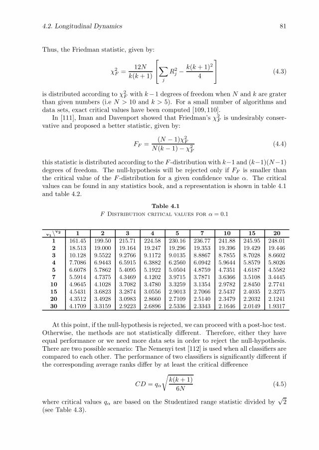
4.2. Longitudinal Dynamics 81
Thus, the Friedman statistic, given by:
χ2F =
12N
k(k + 1)
∑
j
R2j −
k(k + 1)2
4
(4.3)
is distributed according to χ2F with k−1 degrees of freedom when N and k are grater
than given numbers (i.e N > 10 and k > 5). For a small number of algorithms anddata sets, exact critical values have been computed [109,110].
In [111], Iman and Davenport showed that Friedman’s χ2F is undesirably conser-
vative and proposed a better statistic, given by:
FF =(N − 1)χ2
F
N(k − 1) − χ2F
(4.4)
this statistic is distributed according to the F -distribution with k−1 and (k−1)(N−1)degrees of freedom. The null-hypothesis will be rejected only if FF is smaller thanthe critical value of the F -distribution for a given confidence value α. The criticalvalues can be found in any statistics book, and a representation is shown in table 4.1and table 4.2.
Table 4.1
F Distribution critical values for α = 0.1
v1\v2 1 2 3 4 5 7 10 15 20
1 161.45 199.50 215.71 224.58 230.16 236.77 241.88 245.95 248.012 18.513 19.000 19.164 19.247 19.296 19.353 19.396 19.429 19.4463 10.128 9.5522 9.2766 9.1172 9.0135 8.8867 8.7855 8.7028 8.66024 7.7086 6.9443 6.5915 6.3882 6.2560 6.0942 5.9644 5.8579 5.80265 6.6078 5.7862 5.4095 5.1922 5.0504 4.8759 4.7351 4.6187 4.55827 5.5914 4.7375 4.3469 4.1202 3.9715 3.7871 3.6366 3.5108 3.444510 4.9645 4.1028 3.7082 3.4780 3.3259 3.1354 2.9782 2.8450 2.774115 4.5431 3.6823 3.2874 3.0556 2.9013 2.7066 2.5437 2.4035 2.327520 4.3512 3.4928 3.0983 2.8660 2.7109 2.5140 2.3479 2.2032 2.124130 4.1709 3.3159 2.9223 2.6896 2.5336 2.3343 2.1646 2.0149 1.9317
At this point, if the null-hypothesis is rejected, we can proceed with a post-hoc test.Otherwise, the methods are not statistically different. Therefore, either they haveequal performance or we need more data sets in order to reject the null-hypothesis.There are two possible scenario: The Nemenyi test [112] is used when all classifiers arecompared to each other. The performance of two classifiers is significantly different ifthe corresponding average ranks differ by at least the critical difference
CD = qα
√k(k + 1)
6N(4.5)
where critical values qα are based on the Studentized range statistic divided by√
2(see Table 4.3).

82 VALIDATION PROTOCOLS
Table 4.2
F Distribution critical values for α = 0.05
v1\v2 1 2 3 4 5 7 10 15 20
1 39.864 49.500 53.593 55.833 57.240 58.906 60.195 61.220 61.7402 8.5264 8.9999 9.1618 9.2434 9.2926 9.3491 9.3915 9.4248 9.44133 5.5384 5.4624 5.3907 5.3426 5.3092 5.2661 5.2304 5.2003 5.18454 4.5448 4.3245 4.1909 4.1073 4.0505 3.9790 3.9198 3.8704 3.84435 4.0605 3.7798 3.6194 3.5202 3.4530 3.3679 3.2974 3.2379 3.20677 3.5895 3.2575 3.0740 2.9605 2.8833 2.7850 2.7025 2.6322 2.594710 3.2850 2.9244 2.7277 2.6054 2.5216 2.4139 2.3226 2.2434 2.200715 3.0731 2.6951 2.4898 2.3615 2.2729 2.1582 2.0593 1.9722 1.924320 2.9746 2.5893 2.3801 2.2490 2.1582 2.0397 1.9368 1.8450 1.793930 2.8808 2.4887 2.2761 2.1423 2.0493 1.9269 1.8195 1.7222 1.6674
Table 4.3
Critical values for the two-tailed Nemenyi test
# methods 2 3 4 5 6 7 8 9 10
q0.05 1.960 2.343 2.569 2.728 2.850 2.949 3.031 3.102 3.164q0.10 1.645 2.052 2.291 2.459 2.589 2.693 2.780 2.855 2.920
When the aim is to compare the performance of a set of methods against a givenone used as control method, an efficient alternative to Nemenyi test is the Bonferronicorrection or similar procedures. The Nemenyi test adjust the critical value by means
of k(k−1)2 comparisons. However, for comparing a set of methods against a control
method k − 1 comparisons are enough. Although Bonferroni and similar test aregenerally conservative and can have little power, in this case, they are more powerfulthan the Nemenyi test. The test statistics for comparing the i−th and j−th classifierusing these methods is
z =(Ri − Rj)√
k(k+1)6N
(4.6)
The z value is used to find the corresponding probability from the table of normaldistribution, which is then compared with an appropriate α. The tests differ in theway they adjust the value of α to compensate for multiple comparisons.
The Bonferroni-Dunn test [113] controls the family-wise error rate by dividing αby the number of performed comparisons k − 1. The alternative way to computethe same test is to calculate the CD using equation (4.5), but now using the criticalvalues for α
(k−1) (see Table 4.4). The comparison between tables for Nemenyi’s and
Bonferroni-Dunn’s test shows that the power of the post-hoc test is much greaterwhen all classifiers are compared only to a control classifier. We thus should notmake pairwise comparisons when we, in fact, only test whether a newly proposedmethod is better than the existing ones.

4.3. Vessel Structures 83
Table 4.4
Critical values for the two-tailed Bonferroni-Dunn test. The number of
methods include the control method
# methods 2 3 4 5 6 7 8 9 10
q0.05 1.960 2.241 2.394 2.498 2.576 2.638 2.690 2.724 2.773q0.10 1.645 1.960 2.128 2.241 2.326 2.394 2.450 2.498 2.539
4.3 Vessel Structures
In this case, ground truth is given by manual identification of structures in IVUSimages. Since discrepancies among experts provide a non-unique ground truth, wepresent a protocol based on comparisons of inter-observer variability to manual seg-mentations.
4.3.1 Ground truth
The study group has been designed to assess the ability of the reported algorithm todetect the adventitia border in the presence of different plaques, artifacts and vesselgeometries. A total number of 5400 images extracted from 11 different cases havebeen tested. The sequences analyzed are clinical cases of a Boston Scientific ClearView Ultra scanner at 40 MHz with constant pull-back at 0.5 mm/s and acquisitionrate of 25 frames/s from the Hospital Universitari Germans Trias i Pujol in Badalona(Spain). The digitalized sequences are 384 × 288 images with a spatial resolution of0.0435 mm per pixel. We have segmented 22 vessel segments of a length ranging from4 to 6 mm (200-300 frames) and including:
• 6 segments with uncomplete vessel borders due to side-branches and sensorguide shadows.
• 5 calcified segments.
• 9 segments with non calcified plaque.
• 2 normal segments.
For each segment, the adventitia has been manually traced every 10 frames by 4experts in IVUS image interpretation, which yields a total number of 540 validatedframes with 4 different manual models each.
4.3.2 Goodness Measures
To assess segmentation accuracy, the automatically detected borders have been com-pared to the manual models. Accuracy is quantified with the following standardmeasures:

84 VALIDATION PROTOCOLS
1. Absolute and Signed Distances.
Distance maps to manual contours serve to compute the difference in positionbetween automatic and manually traced curves. Such maps encode for eachpixel, p = (xp, yp), its distance to the closest point on the manual contour:
D(p) = minq∈γ(d(p, q)) (4.7)
= minq∈γ
(√(xp − xq)2 + (yp − yq)2
)
where q are points on the manually identified contour. Signed distances (SgnD)[82] weight the value D(p) depending on wether the pixel p lyes inside or outsidethe target curve γ. Its mean value detects any bias in curve position, that is,wether detections are systematically bigger or smaller than manual segmenta-tions.
We will consider absolute (in mm) and relative (in %) distance errors. Absoluteerrors are given by formula (4.7), while relative ones are the ratio:
RelD(p) = 100 · D(p)
d(q, O)
where the origin, O, is the mass center of the manual contour and q is the pointachieving the minimum in (4.7). Since relative errors take into account the truedimensions of the vessel, they reflect positioning errors better.
For each distance error, its maximum and mean values on the automated con-tour are the error measures used to assess position accuracy. If PixSze denotesthe image spatial resolution and p is any point on the automatically tracedadventitia, then the set of functions measuring accuracy in positions are:
• Maximum distance errors (in mm and %):
MaxD = maxp (D(p) · PixSze)RMaxD = maxp (RelD(p))
• Mean distance errors (in mm and %):
MD = meanp (D(p) · PixSze)RMD = meanp (RelD(p))
• Mean signed distance error (in mm):
MSD = meanp (SgnD(p) · PixSze)
2. Area Differences.
Binary images of manual, IM (i, j), and automatic, IA(i, j), borders serve tocompute the following measure for area accuracy:

4.3. Vessel Structures 85
• Percentage of Area Differences
AD = 100 ·∑
i,j |IM (i, j) − IA(i, j)|∑i,j IM (i, j)
The interval given by the mean ± standard deviation computed over the 4 expertscontours indicate the statistical range of values for each of the automated errors(MaxD, RMaxD, MD, RMD and AD).
Inter-observer variability is obtained by computing the error measures for themodels made every two independent observers and it, thus, quantifies discrepancyamong experts. A Student T-test is used to determine if there is any statisticalsignificant difference between inter-observer and automated distance errors average.

86 VALIDATION PROTOCOLS

Chapter 5
Experiments
5.1 In-plane Dynamics
5.1.1 Synthetic Data
Tables 5.1 and 5.2 report the absolute error ranges (E1, E∞) for synthetic motionprofiles. Note that errors do not substantially differ between the two synthetic motionprofiles considered (periodic and quadratic). As expected, error ranges increase intable 5.2 (Sequence Model) as morphological changes appear. Regarding the step,there is no difference in E1 between 1o and 10o. Student (pairwise) t-tests return ap-value equal to 0.99 (CI = (−0.0098, 0.0091)) for Static models and equal to 0.98(CI = (−0.96, 0.95)) for Sequence ones.
Table 5.1
Angle Absolute Error Ranges for Synthetic Profiles - Static Model
1o step 10o step
E1 E∞ E1 E∞
Periodic 0.016 ± 0.081 0.032 ± 0.013 0.016 ± 0.008 0.036 ± 0.017
Quadratic 0.024 ± 0.017 0.051 ± 0.023 0.025 ± 0.013 0.053 ± 0.016
Table 5.2
Angle Absolute Error Ranges for Synthetic Profiles - Sequence Model
1o step 10o step
E1 E∞ E1 E∞
Periodic 2.215 ±0.840 4.904 ±1.446 2.217 ±0.827 4.934±1.417
Quadratic 2.349 ±1.245 5.164 ±1.817 2.366 ±1.316 5.228±1.813
87
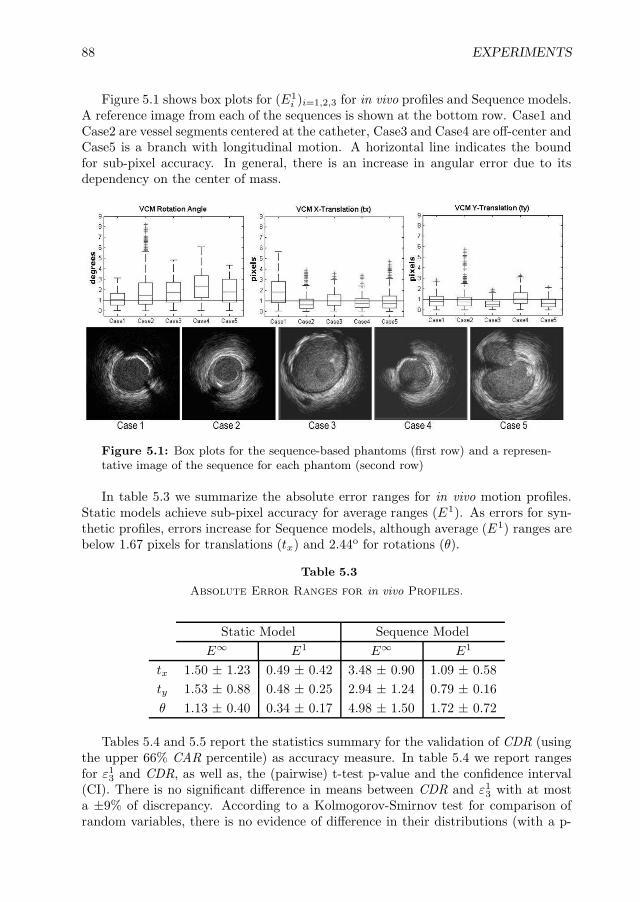
88 EXPERIMENTS
Figure 5.1 shows box plots for (E1i )i=1,2,3 for in vivo profiles and Sequence models.
A reference image from each of the sequences is shown at the bottom row. Case1 andCase2 are vessel segments centered at the catheter, Case3 and Case4 are off-center andCase5 is a branch with longitudinal motion. A horizontal line indicates the boundfor sub-pixel accuracy. In general, there is an increase in angular error due to itsdependency on the center of mass.
Figure 5.1: Box plots for the sequence-based phantoms (first row) and a represen-tative image of the sequence for each phantom (second row)
In table 5.3 we summarize the absolute error ranges for in vivo motion profiles.Static models achieve sub-pixel accuracy for average ranges (E1). As errors for syn-thetic profiles, errors increase for Sequence models, although average (E1) ranges arebelow 1.67 pixels for translations (tx) and 2.44o for rotations (θ).
Table 5.3
Absolute Error Ranges for in vivo Profiles.
Static Model Sequence Model
E∞ E1 E∞ E1
tx 1.50 ± 1.23 0.49 ± 0.42 3.48 ± 0.90 1.09 ± 0.58
ty 1.53 ± 0.88 0.48 ± 0.25 2.94 ± 1.24 0.79 ± 0.16
θ 1.13 ± 0.40 0.34 ± 0.17 4.98 ± 1.50 1.72 ± 0.72
Tables 5.4 and 5.5 report the statistics summary for the validation of CDR (usingthe upper 66% CAR percentile) as accuracy measure. In table 5.4 we report rangesfor ε1
3 and CDR, as well as, the (pairwise) t-test p-value and the confidence interval(CI). There is no significant difference in means between CDR and ε1
3 with at mosta ±9% of discrepancy. According to a Kolmogorov-Smirnov test for comparison ofrandom variables, there is no evidence of difference in their distributions (with a p-

5.1. In-plane Dynamics 89
Table 5.4
CDR vs Angle Relative Error
ε13 CDR p-val CI
Static 95.09 ± 4.63 93.56 ± 4.86 0.3334 (-1.67, 4.73)
Sequence 76.83 ± 13.00 76.59 ± 8.39 0.9545 (-8.60, 9.08)
Table 5.5
CDR vs Other Alignment measures
CDR CC0 CC1 CAR on CC
Static 93.56 ± 4.86 89.27 ± 9.46 93.57 ± 8.43 70.95 ± 21.53
Sequence 76.59 ± 8.39 88.24 ± 6.24 89.58 ± 5.72 28.36 ± 45.63
value of 0.3334 and 0.9545 for Static and Sequence phantoms, respectively). Table5.5 is devoted to comparison of CDR to normalized cross-correlation measures: CC0,CC1 and CAR on CC. Regarding CC, in the absence of morphological changes(Static Model), CC1 and CDR ranges are similar. On Sequence phantoms, thereis no significative difference between CC0 and CC1, which suggests using the CARscore. However, the global nature of CC, makes CAR on CC underestimate theamount of motion suppressed.
Figure 5.2: Linear Correlation between CDR and Angle Relative Accuracy (ε1
3).

90 EXPERIMENTS
Figure 5.2 shows the regression line for the point cloud given by plotting ε13
(X variable) against CDR (Y variable). The regression coefficients for the modelY = b X + a are b = 0.9315 and a = 0.0206. Pearson’s correlation coefficient(ρ) indicates a significant linear dependency (ρ = 0.6611). Finally, the F-statisticsfor testing b = 0 clearly show (with F − pval = 1.1372e−5) that both scores arecorrelated.
5.1.2 In vivo Data
CDR = 89% CDR = 83% CDR = 75% CDR = 63%
(a) (b) (c) (d)
Figure 5.3: Longitudinal cuts for sequences of four different patients (columns),from the best corrected sequence (a) to the worst corrected one (d). Original framesare shown on the first row, original longitudinal cuts on the second row, and correctedones on the third row.
Figure 5.3 shows four cases with decreasing CDR values (from left to right): 89%,83%, 75%, and 63%. The first row shows a frame of the original sequences. Thecorresponding longitudinal cuts at the angles indicated by white lines are shown on thesecond row and the same cut after sequence alignment on the last one. The sequencein the first column (fig.5.3(a)) presents a structure misalignment due to rotation.The calcium shadow appears and disappears in the original longitudinal cut, whereasit shows a uniform appearance after alignment. In the second column (fig.5.3(b))translation introduces a saw-shape in the original longitudinal cut (especially at theend of the segment). After compensation, only a faint undulation due to radial dilationremains. The longitudinal cut in fig.5.3(c) shows a straight profile (both before andafter alignment) in spite of a lower CDR. This phenomenon, which appears in theabsence of motion, is inherent to any relative measure like CDR [107]. Finally, infig.5.3(d) we show the worst performer, both, in terms of longitudinal cut appearanceand CDR value. Since a proper alignment is only achieved at the second half ofthe segment, we have 63% of motion reduction. Regarding objective measurement ofIVUS alignment, we have that the statistical range for CDR gives an overall motionreduction of 82.05%± 6.61%.

5.2. Longitudinal Dynamics 91
5.2 Longitudinal Dynamics
The methodologies were implemented in Matlab code on a Pentium(R) with 3GHzCPU. The average processing time per frame was 36 ms. The set of filters scanned,Gi for gaussian filters and Bi for Butterworth ones is the following.
G1 : σ = 0.001; G2 : σ = 1.5; G3 : σ = 10
B1 : n = 1, δ = 0.5; B2 : n = 1, δ = 0.05; B3 : n = 1, δ = 0.005;B4 : n = 2, δ = 0.5; B5 : n = 2, δ = 0.05; B6 : n = 2, δ = 0.005;B7 : n = 4, δ = 0.5; B8 : n = 4, δ = 0.05; B9 : n = 4, δ = 0.005
Tables 5.6 and 5.7, report the average ranks reflecting each filter performance (thesmaller, the better).
Table 5.6
Average Rank of the Gaussian Filters with parameters given by σ for Nemenyi
Test
σ 0.001 1.5 10
Rank 9.43 4.71 5.75
Table 5.7
Average Rank of the Butterworth Filters with parameters given by (n, δ) for
Nemenyi Test
n\δ 0.5 0.05 0.005
1 4.93 4.71 8.12
2 5.28 4.96 8.62
4 5.81 6.18 9.43
For a significance level of 0.1, the Nemenyi critical difference (CD) is 3.86. Thetest detects that Butterworth filters with n = 1, 2, 4, δ = 0.005 (B3, B6 and B9) andGaussian with σ = 0.001 (G1), which are too restricted around ωc, are significantlyworst. The Nemenyi test also reports that there is not enough evidence of a signif-icantly different performance among the remaining methods. Figure 5.4 shows therank of filters from right to left (the best is on the right) together with the criticaldifference in order to visually compare all filters. There are two distinguished sets,but there are no significative differences between the filters in each set. Table 5.8reports the ranges, by the mean ± the variance (σ ± µ) of the filters of the set withbetter ranks. Values in the first column are in frames, the ones of the second column

92 EXPERIMENTS
Figure 5.4: Comparison of different filters using the Nemenyi test.
are in seconds and the last column correspond to the values in millimeters. As fig-ure 5.4 shows, there is no significative difference between them. The Gaussian filterwith σ = 1.5 achieves the best results with an error within 3.26± 1.55 frames, whichcorresponds to 0.05 ± 0.03 mm.
Table 5.8
Average Errors of the best set of filters
Method Frames Seconds MillimetersG2 3.2580± 1.5458 0.1086± 0.0515 0.0543± 0.0258G3 3.5499± 1.5352 0.1183± 0.0512 0.0592± 0.0256B1 3.4336± 1.6755 0.1145± 0.0558 0.0572± 0.0279B2 3.4455± 1.7838 0.1148± 0.0595 0.0574± 0.0297B4 3.3620± 1.7163 0.1121± 0.0572 0.0560± 0.0286B5 3.5272± 1.7959 0.1176± 0.0599 0.0588± 0.0299B7 3.4065± 1.7005 0.1136± 0.0567 0.0568± 0.0283B8 3.6655± 1.8971 0.1222± 0.0632 0.0611± 0.0316
Figure 5.5 shows an example of the automatic sampling on a real longitudinal cut.The top image is a longitudinal cut of 42 mm. long showing a side branch on theupper half. The left bottom image shows the image-based ECG sampling in dashedlines at the side branch segment. The right bottom image shows the longitudinal cutsampled at end diastole rate.
Figure 5.6 shows the performance of our method for the Gaussian filtering in 2large longitudinal cuts. The original cuts are in the left, while the cuts sampled atend diastole rate are in the right. For the first segment, we can notice the continuousprofile for the lumen contour, while in the second segment, we can follow up thecalcium plaque present in the vessel.

5.2. Longitudinal Dynamics 93
Figure 5.5: Image-based ECG sampling on a longitudinal cut.
Figure 5.6: Results of Image-based ECG sampling for two different longitudinalcuts.

94 EXPERIMENTS
5.3 Vessel Structures
The set of optimal parameters for a Boston Clear View is given by:
PF1 = 0.1906X + 0.9817Y
with thresholding parameters set to:
τPF1 = 0.0567; ρX = 6%; ρF = 85%
for computation of vessel borders mask and
PF2 = −0.1498PF1 + 0.9887Z, τPF2 = −0.1241
for the calcium mask. The adventitia detection parameters ensure a 99.95% of trueC1 detections. We note that, by the feature space definition, we only have a 17% offalse positives, which just represent 6% of the total number of points classified in C1.This fact favors the use of a length filtering on adventitia detections as fake responseremover. In the case of calcium extraction, the threshold achieves less than a 1% ofnoise and ensures 90.2156% of calcium detections. For the computation of the finalB-snake model we have used 30 control points uniformly placed every 12 angles.
We have analyzed errors individually for each patient gathered by vessel plaquenature and globally. Whisker boxes are usual to analyze within patient variability andconfident intervals serve to detect any significant difference between different plaques.
Figure 5.7 shows whisker boxes for mean distance absolute errors (top plot) andmean inter-observer variations (bottom plot) for soft plaque and calcium segments.Each box contains the mean distance errors obtained from the 4 experts segmenta-tions (80 to 120 samples per box) for a single vessel segment. Boxes labeled withNC correspond to non-calcified segments and those labeled with C to calcified ones.An analysis of the whisker boxes reflects robustness of segmentations: the smaller theboxes are, the more reliable the method is. Whisker boxes serve to visually detect anyanomaly in the models. In general terms, the means of automated errors are slightlyhigher than inter-observer variability means. However, since automatic segmenta-tions present a significantly smaller variation range than inter-observer variability,our segmentations are within the experts discrepancy rate (see T-tests comparingmeans summarized in table 5.12. Lack of reliable information at large angular sec-tors, significantly increases errors variability in calcified segments,both for manualsegmentations and automatic detections. The large range of the whisker box of thecase C2 detects it as a vessel segment of difficult manual identification that should beexcluded from any statistical analysis. Larger boxes for automated detections (top)in cases NC5 and C3 comparing to their counterparts (bottom) indicate that thereare specially difficult cases for our segmenting strategy. At the end of the section, adetailed analysis of such miss detections is done.
Statistical ranges (mean ± standard deviation) for automatic errors (AUT) andinter-observer variability (INT-OBS) are summarized in tables 5.9, 5.10, and 5.11.Patients presenting an unusual large inter-observer variability have been excluded,since we consider they are anomalous cases with difficult and non robust manual
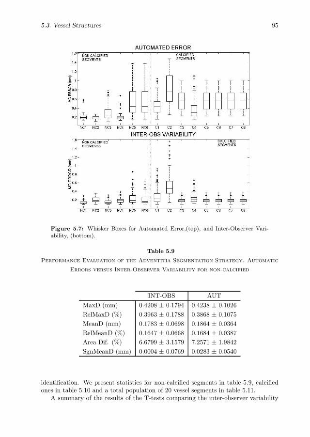
5.3. Vessel Structures 95
Figure 5.7: Whisker Boxes for Automated Error,(top), and Inter-Observer Vari-ability, (bottom).
Table 5.9
Performance Evaluation of the Adventitia Segmentation Strategy. Automatic
Errors versus Inter-Observer Variability for non-calcified
INT-OBS AUT
MaxD (mm) 0.4208 ± 0.1794 0.4238 ± 0.1026
RelMaxD (%) 0.3963 ± 0.1788 0.3868 ± 0.1075
MeanD (mm) 0.1783 ± 0.0698 0.1864 ± 0.0364
RelMeanD (%) 0.1647 ± 0.0668 0.1684 ± 0.0387
Area Dif. (%) 6.6799 ± 3.1579 7.2571 ± 1.9842
SgnMeanD (mm) 0.0004 ± 0.0769 0.0283 ± 0.0540
identification. We present statistics for non-calcified segments in table 5.9, calcifiedones in table 5.10 and a total population of 20 vessel segments in table 5.11.
A summary of the results of the T-tests comparing the inter-observer variability

96 EXPERIMENTS
Table 5.10
Performance Evaluation of the Adventitia Segmentation Strategy. Automatic
Errors versus Inter-Observer Variability for calcified segments
INT-OBS AUT
MaxD (mm) 0.6627 ± 0.3610 0.7161 ± 0.2532
RelMaxD (%) 0.5469 ± 0.3171 0.6116 ± 0.2665
MeanD (mm) 0.2650 ± 0.1306 0.2885 ± 0.0947
RelMeanD (%) 0.2142 ± 0.1113 0.2388 ± 0.0931
Area Dif. (%) 9.3511 ± 5.7529 10.0428 ± 4.0390
SgnMeanD (mm) 0.0163 ± 0.1213 -0.0381 ± 0.0912
Table 5.11
Performance Evaluation of the Adventitia Segmentation Strategy. Automatic
Errors versus Inter-Observer Variability for all segments
INT-OBS AUT
MaxD (mm) 0.5386 ± 0.3075 0.5715 ± 0.2296
RelMaxD (%) 0.4697 ± 0.2664 0.5122 ± 0.2344
MeanD (mm) 0.2206 ± 0.1126 0.2265 ± 0.0688
RelMeanD (%) 0.1888 ± 0.0945 0.1972 ± 0.0662
Area Dif. (%) 7.9813 ± 4.7962 8.6032 ± 3.3436
SgnMeanD (mm) 0.0081 ± 0.1013 0.0041 ± 0.0801
and automatic errors averages is given in table 5.12. We report the p-value and theconfidence interval for the difference in means. Statistics exclude outliers and T-testsare computed over the total errors in table 5.11.
According to a two tailed T-test, there is no significant difference between inter-observer and automated mean absolute distance errors and difference in areas. Formean distance errors the p-value equals p = 0.177721 and the confidence interval forthe true difference in means at a significance level of 95% is CI = (−0.002684, 0.014491).In the case of percentage in area difference, p = 0.153404 and the interval (also at asignificance level of 95%) is CI = (−0.017985, 0.114350). Maximum errors for auto-mated detections are slightly above the range of maximum inter-observer variability.In order to robustly determine the fraction of increase, we use a single tailed T-testto check if the null hypothesis statement ”the mean of automated maximum errorsis above λ times the mean of maximum inter-observer variabilities” is true. The trueproportion between maximum automated error and inter-observer variability is be-

5.3. Vessel Structures 97
Table 5.12
Statistics Summary on T-tests comparing the means of Inter-Observer
Variability and Automatic Errors.
Confidence Interval (CI) p-value
MeanD (-0.002684,0.014491) 0.177721
Area Dif. (-0.017985,0.114350) 0.153404
SgnMeanD (-0.002401,0.010787) 0.212219
tween the minimum λ rejecting the null hypothesis and the maximum accepting it.For λ = 1.102, the null hypothesis was accepted with a p-value, p = 0.053901 andfor λ = 1.103, it was rejected with p = 0.049846. We conclude that the increasein maximum automated errors is under a 10.3%. Finally a T-test on the mean ofthe automated signed distance error shows that in average it is zero as the p-valueequals p = 0.212219 and the confidence interval for the true mean is a tiny intervalcontaining the zero value CI = (−0.002401, 0.010787).
Some of the adventitia segmentations achieved with the presented strategy areshown in the next figures. We split them in four different cases: the first (figure 5.8)corresponds to normal vessel segments, the second (figure 5.9) to vessel segments withsoft plaque. The third (figure 5.10) have been extracted from calcified vessel segmentsand finally, the last one (figure 5.11) shows images with missing information, mainlydue to side branches and sensor guide shadows.
1. NORMAL SEGMENTS In the first column we present a normal segment,whereas in the second one, the vessel presents non-fibrous plaque.
2. SOFT PLAQUE SEGMENTS In the first column, we present a vessel segmentwith lipidic plaque, whereas, in the second column, the vessel segment con-tains soft plaque. Notice that in the anisotropic contour closing step (fig.5.9(l)to fig.5.9(m)) we use image borders continuity, since these images come fromcartesian coordinates. Thus, although adventitia points before the ACC do notappear on the right of the image, ACC closes in the two directions from the leftside of the image.
3. CALCIFIED PLAQUE SEGMENTS In this case, both vessels contain calcifiedplaque. Notice that, although intima is detected, both polar coordinates and arigid snake, yield that the final closed model corresponds to the adventitia.
4. SIDE BRANCHES AND SENSOR SHADOW SEGMENTS Both vessel seg-ments lack of information, the first due to a calcified area plus a side branchand the second column, because of sensor shadow and a little side branch. Thekey point of this kind of images is the sparse information, which we discuss inthe next subsection.

98 EXPERIMENTS
(a) (h)
(b) (i)
(c) (j)
(d) (k)
(e) (l)
(f) (m)
(g) (n)
Figure 5.8: Automated Adventitia Detections for Normal Vessel Segments

5.3. Vessel Structures 99
(a) (h)
(b) (i)
(c) (j)
(d) (k)
(e) (l)
(f) (m)
(g) (n)
Figure 5.9: Automated Adventitia Detections for Vessel Segments with Soft Plaque

100 EXPERIMENTS
(a) (h)
(b) (i)
(c) (j)
(d) (k)
(e) (l)
(f) (m)
(g) (n)
Figure 5.10: Automated Adventitia Detections for Calcified Vessel Segments

5.3. Vessel Structures 101
(a) (h)
(b) (i)
(c) (j)
(d) (k)
(e) (l)
(f) (m)
(g) (n)
Figure 5.11: Automated Adventitia Detections for Uncomplete Vessel Segments

102 EXPERIMENTS
5.4 Discussion
By combining vessel appearance and shape, we provide explicit formulae for rigidin-plane motion parameters. This sets no limits to the capture range of motion pa-rameters and we have equal performance (tables 5.1 and 5.2) for frame-to-frame stepsof 1o and 10o. Translation is given (independently for each frame) in absolute terms,whereas rotation is computed by accumulating frame-to-frame transformations. Inlarge segments, the latter might introduce accumulation errors. Alignment of largesegments is a difficult task, due to morphological variations, which also might dropthe accuracy of registration algorithms. Therefore, we consider that this does notrepresent a major limitation of our approach compared to registration strategies. Ex-periments on sequence-based synthetic models (table 5.3) show that the main sourceof error arises from morphological changes along the vessel, with average errors of1.09 pixels ∗ 0.04 mm/pixel = 0.044mm for translations and 1.72o for rotations. Ourerrors favorably compare to the numbers reported in [114], which achieve mean errorsof 0.064mm and 7.8o, provided that the catheter rotation does not exceed 5o.
Our quality measure, CDR, bases on the conservation of the image local densityof mass (given by the local mean) and only considers image pixels with noticeablemotion. Results on Sequence models (table 5.4) show that CDR correlates to theangular relative accuracy. Results on real pullbacks show that, in general, CDR alsocorrelates to the uniform and continuous appearance of longitudinal cuts (see figure5.3(a), (b), and (d)). This fact validates CDR as an objective measure of imagealignment. Comparison to global similarity scores, such as cross-correlation (table5.5), indicates that global approaches are prone to underestimate motion reduction.
Experimental results detect two sources for under performance of the proposedmethodology: sudden morphological changes and non-periodic random motion pat-terns. In the first case, which is a common limitation in most registration and track-ing algorithms, changes in appearance mislead image alignment as the objects to betracked have significantly changed. The second source of error is inherent to thedefinition of rigid (periodic) movement, which is the only motion considered. Theseextreme cases, which CDR might drop to 63%, only represent a 6% of the data ana-lyzed.
Regarding longitudinal dynamics assessment, cardiac phase can be strongly af-fected by artery lesions and other cardiac factors. Thus, the strategy used to retrieveit has to be accurately chosen. We propose two different methods for extracting car-diac signal and a battery of filters to remove noise and other non-cardiac phenomena.Local approaches allow simple quantities (e.g. image intensity) efficiently (36ms perframe) retrieve an accurate cardiac phase. Band pass filters support should not betoo restricted around ωc in order to avoid uniform samplings. For segments of ap-proximately 1 cm average length, the decay of Gaussian filters is better suited withan error within 0.054± 0.025 mm.
Finally, the reliability of the proposed strategy for adventitia segmentation isreflected in the global statistics extracted from in vivo sequences segmentation. Thefact that, both, mean distances and vessel areas compare to inter-observer variationvalidates our method for extraction of clinical measurements. Since there is no biasin automated segmentations (the mean signed distance is statistically zero) we can

5.4. Discussion 103
ensure that our method achieves an optimal compromise among experts criteria asautomatically traced curves lie between the curves traced by different observers. Thenumber of outlier bad segmentations requiring manual correction represent less thana 15% of the studied valid cases.
Still, the striking increase in the error range for the anomalous cases NC5 and C3needs to be analyzed. Such miss detections correspond to vessel segments that eitherthe adventitia is hardly identified or there is severe lack of valid information.
Weak visual appearance of the adventitia border is a technical limitation of theUltraSound acquisition technique and it is cause of disagreement among experts (caseC2 in fig.5.7(b)) in 9% of the cases. Our strategy suffers this kind of error in 18%of the segments under study (boxes C5, NC2 and NC3 in fig.5.7(a)). We argue thatthe only way to minimize the impact of border blurring is taking into account tissuemotion periodicity along the sequence. Even for physicians it is difficult to identifyvessel borders by an analysis of still images. Often, they use cardiac periodicity inthe movement of vessel structures to distinguish between tissue and other structures.
(a) (b) (c)
(d) (e) (f)
Figure 5.12: Adventitia models in images with sparse information. Points detected(a), (d), final snake (b), (e) and manual model (c), (f).
The second source of large error in automatic detections is lack of information.Calcium sectors or side branches can take up large angular sectors, thus, distortinginformation at these sectors. In the case that the sparse valid information is not uni-formly distributed along angular sectors, the final model is prone to underestimate

104 EXPERIMENTS
the border true radial position. Fig.5.12 illustrates the scarce bad distributed infor-mation artifact. On the first column we show an image with uniformly enough pointdistribution and on the second column a pathological case with all available infor-mation gathered in the first quadrant of the image. Images in fig.5.12(a), (d) depictthe ACC closure modeled by the B-snake in fig.5.12(b), (e). The reference manuallytraced contours are shown in fig.5.12(c), (f).
We note that it is reported in the literature [84] that measurements should notbe reported if lack of information is more extensive than 90 of arc. Still our erroranalysis prompts that lack of strong 3D continuity in the B-snake closing of candidatepoints on the vessel borders is the main source of the above error. The use of 2DNURBS (spline surfaces) instead of 1D splines could reduce the impact of missinginformation. However, in our case, they might not succeed in correcting this kind ofmiss interpolations. On one hand, NURBS can only take into account local defor-mations and continuity of the surface. On the other hand, the previously describedpathology is prone to happen at large vessel segments. It follows that NURBS inter-polation might imply handling the segmentation of the whole image sequence block(over 1200 frames), which is computationally unfeasible. One possible way of over-coming lack of information for large vessel segments would be mimicking the expertsstrategy used for manually tracing the adventitia borders. Our application [115] tomanually segment vessel borders shows the previous border on the current image tobe segmented and allows the physician to modify it. An informal survey on the keypoints and frames used by the expert for border tracing at images with severe lack ofinformation prompts that they usually keep the model traced on the last valid frame.This suggests using the information available at the last frame with adventitia pointsdetected in more than 70% of the vessel angular sectors to complete vessel borders atimages with sparse detections.

Conclusions and Further
Lines
Image processing methodologies are becoming an important tool for using IntraVas-cular UltraSound for the diagnosis, treatment, and intervention of cardiovasculardiseases. In this work we have approached three main challenging problems: rigidin-plane dynamics suppression, cardiac phase retrieval, and vessel-structures segmen-tation.
Rigid in-plane dynamics: We have described a method for estimating andcompensating rigid in-plane dynamics. We have provided explicit formulae for motionparameters by combining vessel appearance and shape. Fourier development hasshown to be a reliable tool for estimating rotation between consecutive frames as faras translation is well-estimated. As well, we have decomposed the rotation profile intoits three main contributions: cardiac signal, breathing and geometric components.Results on synthetic experiments and in vivo segments show that the methods aresuitable for exploring tissue bio-mechanical properties from in vivo clinical cases.
Longitudinal Dynamics: We have presented a methodology for retrieving car-diac phase from sequences without ECG signal. We have presented two differentapproaches to extract cardiac signal from IVUS sequences, as well as two familiesof filters for removing non-cardiac frequencies. On one hand, exploring LM evolu-tion is a fast way to extract cardiac signal from IVUS sequences. On the other one,the profiles obtained from estimating cardiac rotation show that the algorithm seemsto be a good candidate for globally retrieving cardiac signal. Regarding the filtersused Band-pass filters support should not be too restricted around the main cardiacharmonic in order to avoid uniform samplings. For segments of approximately 1 cmaverage length, the decay of Gaussian filters is better suited.
Structures exploring: We have presented a statistical-deterministic strategyfor detecting vessel borders in IVUS sequences. The combination of a priori knowl-edge (classification techniques) with filtering techniques based on continuity of imagegeometry has proven to be the key point for a robust characterization of vessel (theadventitia layer, in our case) borders. Once again, rigid in-plane dynamics estimationseems to be a straightforward method for previously filtering the sequence, althoughit can be less precise. By designing an accurate point selection strategy, we avoidhuman interaction and the use of longitudinal cuts and ECG-gated acquisitions.
105

106 CONCLUSIONS AND FURTHER LINES
Validation Protocols: Since validation is an essential part of any algorithmfor ensuring a wide clinical applicability, we have taken special care in designing avalidation protocol for each contribution. As well, since there is no objective measurefor dynamics assessment in in vivo sequences, we have described a quantitative scoreto objectively assess the amount of motion suppressed.
Further Lines
The methods proposed in this PhD thesis pave the way for several studies.
1. Vessel bio-mechanical properties: Tissue bio-mechanical properties is anactive research area due to its prediction potential. The main artifact hinderingits assessment in coronary arteries is the in-plane rigid motion. Once the se-quences are stabilized, tissue bio-mechanical properties can be investigated byapplying an elastic motion estimation on segments with uniform kind of plaques.Furthermore, blood flow can also be explored as far as pixel precision allows toobserve significant changes along the sequence.
2. Objective validation of Longitudinal Dynamics: Lumen area changes arerelated to cardiac phenomena, and its comparison to automated sampling en-couraging. Nevertheless, samplings obtained from ECG signals are an objectiveground truth for validating the method for retrieving cardiac phase.
3. 3D Reconstruction: Although 3D reconstruction only from IVUS sequences isnot feasible without an external reference system, segmentation of vessel struc-tures is a first step towards the next dimension
4. Structures and dynamics exploring workstation: Rigid motion estima-tion seems to be a useful algorithm for exploring both, structures and cardiacdynamics. Preliminary results encourage an exhaustive validation for the assess-ment of motion estimation as the basis of a framework exploring vessel dynamicsand structures. It would increase the computation efficiency of a workstationfor helping physicians in diagnosing and treating cardiovascular diseases.

Publications
Journal Papers
• A. Hernandez-Sabate, D. Gil, E. Fernandez-Nofrerias, P. Radeva, E. Martı,“Approaching Artery Rigid Dynamics in IVUS”, IEEE Transactions on MedicalImaging, in press.
• D. Gil, A. Hernandez, J. Mauri, P. Radeva, “A Deterministic-Statistic Strategyfor Media-Adventitia Border Modeling in IVUS sequences”, IEEE Transactionson Medical Imaging , vol. 25, n.6, June 2006.
• O. Rodrıguez, J. Mauri, E. Fernandez, A. Tovar, V. Valle, A. Hernandez, D.Gil, P. Radeva, “Utilizacion de la estructura de los campos vectoriales parala deteccion de la adventicia en imagenes de ecografıa intracoronaria”, RevistaEspanola de Cardiologıa , Octubre 2004; vol. 57(Supl. 2), pg. 100.
• O. Rodrıguez, A. Carol, H. Tizon, E. Fernandez, J. Mauri, V. Valle, D. Gil, A.Hernandez, P. Radeva, “ Model estadıstic-determinıstic per la segmentacio del’adventıcia en imatges d’ecografia intracoronaria ”, Rev. Soc. Cat. Cardiol.Vol. 5, no4, supl., pag. 41.
Conference papers
• Debora Gil, Aura Hernandez-Sabate, Mireia Brunat, Jordi Martınez-Vilalta,Steven Jansen, ”Structure-Preserving Smoothing of Biomedical Images”, InProc. of the 13th International Conference on Computer Analysis of Imagesand Patterns (CAIP’2009) , Munster, Germany, September 2009, accepted.
• Aura Hernandez-Sabate, David Rotger, Debora Gil, ”Image-based ECG Sam-pling of IVUS Sequences”, In Proc. of the 2008 IEEE International UltrasonicsSymposium , Beijing, November 2008, pp. 1330-1333.
• Debora Gil, Petia Radeva, Oriol Rodriguez-Leor, Aura Hernandez, “AssessingArtery Motion Compensation in IVUS”, In Proc. of the 12th International Con-ference on Computer Analysis of Images and Patterns (CAIP’2007) , Vienna,Austria, August 2007. LNCS 4673, pp. 213-220.
107

108 PUBLICATIONS
• Aura Hernandez, Oriol Rodriguez, Debora Gil, “Quantitative Assessment ofArtery Motion Compensation in IVUS Sequences”, In Computer Vision: Ad-vances in Research and Development. Proc. of the 2nd CVC InternationalWorkshop (CVCRD ’07), Bellaterra (Spain), October 2007, pp. 83-88.
• Aura Hernandez, Debora Gil, “ How Do Conservation Laws Define A MotionSuppression Score in in-vivo IVUS Sequences? ”, In Proc. of the 2007 IEEEInternational Ultrasonics Symposium , New York, October 2007, pp. 2231-2234.
• F. Guirado, A. Ripoll, C. Roig, A. Hernandez, E. Luque, “Exploiting throughoutfor pipeline execution in streaming image processing applications”, Euro-Par2006, Parallel Processing, 12th International Euro-Par Conference , LNCS 4128, Dresden, Germany, Sept. 2006, pp. 1095-1105.
• A. Hernandez, D. Gil, J. Mauri, P. Radeva, “Reducing Cardiac Motion in IVUSSequences”, Computers in Cardiology 2006 , Valencia, Spain, 2006, pp. 685-688.
• A. Hernandez, P. Radeva, A. Tovar, D. Gil, “Vessel Structures Alignment bySpectral Analysis of IVUS Sequences”, The 1st International Workshop on Com-puter Vision for Intravascular and Intracardiac Imaging , MICCAI, 2006, pp.29-36.
• P. Fritzsche, C. Roig, A. Ripoll, E. Luque and A. Hernandez, ”A PerformancePrediction Methodology for Data-dependent Parallel Applications”, In IEEEInternational Conference on Cluster Computing, September 2006, pp. 1-8.
• D. Gil, A. Hernandez, A. Carol, O. Rodrıguez, P. Radeva, “ A deterministic-statistic adventitia detection in IVUS images”, Functional Imaging and Mod-eling of the Heart 2005, LNCS 3504, Barcelona, Spain, June 2:4, pp. 65—74,2005 .
• A. Hernandez, D. Gil, P. Radeva, “On the usefulness of supervised learning forvessel border detection in IntraVascular Imaging”, Frontiers in artificial intelli-gence and applications, IOS Press, pp 67—74, 2005.
• O. Rodrıguez, J. Mauri, E. Fernandez, A. Carol, V. Valle Tudela, D. Gil, A.Hernandez, P. Radeva., “ A deterministic-statistic adventitia modeling IVUSimages ”, ESC Congress 2005 , Stockholm.
• A. Hernandez, D. Gil, P. Radeva , “Anisotropic Processing of Image Structuresfor Adventitia Detection in intravascular Ultrasound Images”, Computers inCardiology, vol. 31, pp. 229-232, Chicago (USA).
Technical Reports
• A. Hernandez, D. Gil, P. Radeva, ”A Deterministic-Statistical Strategy for Ad-ventitia Segmentation in IVUS images”, CVC Tech. Report n 89 , August 2005.
• A. Hernandez, “ Automatic adventitia segmentation in IntraVascular Ultra-Sound images” , CVC Tech. Report, n85, August 2005.

Bibliography
[1] V. Fuster, “Mechanisms leading to myocardial infarction: Insights from studiesof vascular biology,” Circulation, vol. 90, no. 4, pp. 2126–2146, October 1994.
[2] I. Kakadiaris, S. O’Malley, M. Vavuranakis, S. Carlier, R. Metcalfe, C. Hartley,E. Falk, and M. Naghavi, “Signal-processing approaches to risk assessment incoronary artery disease,” IEEE Signal Processing Magazine, vol. 23, no. 6, pp.59–62, Nov. 2006.
[3] E. Cespedes, C. Korte, and A. van der Steen, “Intraluminal ultrasonic palpa-tion: assessment of local cross-sectional tissue stiffness,” Ultrasound Med. Biol.,vol. 26, pp. 385–396, March 2000.
[4] J. Wentzel, R. Krams, J. H. Schuurbiers, J. Oomen, J. Kloet, W. van derGiessen, P. Serruys, and C. Slager, “Relationship between neointimal thick-ness and shear stress after wallstent implantation in human coronary arteries,”Circulation, vol. 103, no. 13, pp. 1740–5, 2001.
[5] D. Cavaye, R. White, K. GE et al., “Intravascular ultrasound imaging: Thenew standard for guidance and assessment of endovascular interventions,” JClin Laser Med Surg, vol. 10, no. 5, pp. 3349–353, 1992.
[6] I. Fontaine, M. Bertrand, and G. Cloutier, “A system-based approach to mod-elling the ultrasound signal backscattered by red blood cells,” Biophysical Jour-nal, vol. 77, no. 5, pp. 2387–2399, 1999.
[7] M. Rosales, P. Radeva, J. Mauri, and O. Pujol, “Simulation model of intravas-cular ultrasound images,” in MICCAI, vol. 3217, Sept. 2004, pp. 200–7.
[8] G. Mintz, S. Niessen, W. Anderson, S. Bailey, R. Erbel, P. Fitzgerald, F. Pinto,K. Rosenfield, R. Siegel, E. Tuzcu, and P. Yock, “Acc clinical expert consensusdocument on standards for acquisition, measurement and reporting of intravas-cular ultrasound studies (IVUS),” Journal of the American College of Cardiol-ogy, vol. 37, no. 5, pp. 1478–92, 2001.
[9] A. Arbab-Zadeh, A. DeMaria, W. Penny, R. Russo, B. Kimura, and V. Bhar-gava, “Axial movement of the intravascular ultrasound probe during the cardiaccycle: implications for three-dimensional reconstruction and measurements ofcoronary dimensions,” Am. Heart J., vol. 138, pp. 865–872, 1999.
109

110 BIBLIOGRAPHY
[10] P. Delachartre, C. Cachard, G. Finet, F. Gerfault, and D.Vray, “Modeling ge-ometric artefacts in intravascular ultrasound imaging,” Ultrasound Med. Biol.,vol. 25, no. 4, pp. 567–575, May 1999.
[11] N. Bruining, C. von Birgelen, P. J. de Feyter, J. Ligthart, W. Li, P. Serruys,and J. R. Roelandt, “ECG-gated versus nongated three-dimensional intracoro-nary ultrasound analysis: Implications for volumetric measurements,” CatheterCardiovasc. Diagn., vol. 43, no. 3, pp. 254–260, Mar. 1998.
[12] C. von Birgelen, G. Mintz, A. Nicosia, D. P. Foley, W. J. van der Giessen,N. Bruining, S. Airiian, J. T. C. Roelandt, P. de Feyter, and P. Serruys,“Electrocardiogram-gated intravascular ultrasound image acquisition after coro-nary stent deployment facilitates on-line three-dimensional reconstruction andautomated lumen quantification,” J. Amer. Coll. Cardiol., vol. 30, no. 2, pp.436–443, Aug. 1997.
[13] S. Winter, R. Hamers, M. Degertekin, K.Tanabe, P. Lemos, P. Serruys, J. R.Roelandt, and N. Bruining, “Retrospective image-based gating of intracoronaryultrasound images for improved quantitative analysis: The intelligate method,”Catheter Cardiovasc. Interv., vol. 61, no. 1, pp. 84–94, Jan. 2004.
[14] A. Wahle, S. C. Mitchell, S. D. Ramaswamy, K. Chandran, and M. Sonka,“Four-dimensional coronary morphology and computational hemodynamics,” inSPIE Medical Imaging 2001: Image Processing Conference, vol. 4322, February2001, pp. 743–754.
[15] S. . Nadkarni, D. . Boughner, and A. . Fenster, “Image-based cardiac gating forthree-dimensional intravascular ultrasound imaging,” Ultrasound in Medicineand Biology, vol. 31, no. 1, pp. 53–63, 2005.
[16] H. Zhu, K. D. Oakeson, and M. H. Friedman, “Retrieval of cardiac phase fromIVUS sequences,” in Medical Imaging 2003: Ultrasonic Imaging and SignalProcessing, vol. 5035, 2003, pp. 135–146.
[17] M. M. S. Matsumoto, P. A. Lemos, T. Yoneyama, and S. S. Furuie, “Cardiacphase detection in intravascular ultrasound images,” in Medical Imaging 2008:Ultrasonic Imaging and Signal Processing, February 2008.
[18] I. A. K. Sean M. O’Malley, Morteza Naghavi, “Image-based frame gating forcontrast-enhanced IVUS sequences,” in International Workshop on ComputerVision for Intravascular and Intracardiac Imaging, International Workshop onCVIII, MICCAI, 2006.
[19] J. Barajas, K. L. Caballero, O. Rodriguez, and P. Radeva, “Cardiac phaseextraction in IVUS sequences using 1-D gabor filters,” in 29th Annual Interna-tional Conference of the IEEE EMBS, August 2007.
[20] J. Shaw, B. Kingwell, A. Walton, J. Cameron, P. Pillay, C. Gatzka, and A. Dart,“Determinants of coronary artery compliance in subjects with and without an-giographic coronary artery disease,” JACC, vol. 39(10), pp. 1637–1643, 2002.

BIBLIOGRAPHY 111
[21] S. Nadkarni, H. Austin, and et al., “A pulsating coronary vessel phantom fortwo and three-dimensional intravascular ultrasound studies.” Ultrasound Med.Biol., vol. 29, no. 4, pp. 621–628, 2003.
[22] K. Y. E. Leung, R. Baldewsing, F. Mastik, J. Schaar, and D. Gisolf, “Motioncompensation for intravascular ultrasound palpography,” IEEE Trans. UFFC,vol. 53, pp. 1269–1280, 2006.
[23] A. Jeremias, C. Spies, N. A. Herity, E. Pomerantsev, P. G. Yock, P. J. Fitzgerald,and A. C. Yeung, “Coronary artery compliance and adaptive vessel remodellingin patients with stable and unstable coronary artery disease,” Heart, vol. 84,pp. 314–319, 2000.
[24] C. L. de Korte, G. Pasterkamp, A. F. van der Steen, H. A. Woutman, andN. Bom, “Characterization of plaque components with intravascular ultrasoundelastography in human femoral and coronary arteries in vitro,” Circulation, vol.102, pp. 617–623, 2000.
[25] Y. Shi, F. de Ana, S. Chetcuti, and M. O’Donell, “Motion artifact reduction forIVUS-based thermal strain imaging,” IEEE Trans. Ultrason. Ferroelect. Freq.Contr., vol. 52, pp. 1312–1319, August 2005.
[26] M. Danilouchkine, F. Mastik, and A. van der Steen, “A study of coronaryartery rotational motion with dense scale-space optical flow in intravascularultrasound,” Phys. Med. Biol., vol. 54, pp. 1397–1418, February 2009.
[27] Y. Saijo, A. Tanaka, N. Owada, Y. Akino, and S. Nitta, “Tissue velocity imag-ing of coronary artery by rotating-type intravascular ultrasound,” Ultrasonics,vol. 42, pp. 753–757, 2004.
[28] B. Zitova and J. Flusser, “Image registration methods: a survey,” Image VisionComput., vol. 21, no. 11, pp. 977–1000, Oct. 2003.
[29] A. Hernandez, P. Radeva, A. Tovar, and D. Gil, “Vessel structures alignmentby spectral analysis of IVUS,” in Computer Vision for Intravascular Imaging,Oct. 2006, pp. 30–37.
[30] J. Dijkstra, G. Koning, J. Tuinenburg, P. Oemrawsingh, and J. Reiber, “Au-tomatic border detection in intravascular ultrasound images for quantitativemeasurements of the vessel, lumen and stent parameters,” in Computer As-sisted Radiology and Surgery - CARS 2001, 2001, pp. 916–922.
[31] C. von Birgelen, C. Mario, W. Li, J. Schuurbiers, C. Slager, P. de Feyter,J. Roelandt, and P. Serruys, “Morphometric analysis in three-dimensional in-tracoronary ultrasound: An in vitro and in vivo study performed with a novelsystem for the contour detection of lumen and plaque,” Am. Heart Journal, vol.132, pp. 516–527, 1996.
[32] C. von Birgelen, G. S. Mintz, A. Nicosia, D. P. Foley, W. J. van der Giessen,N. Bruining, S. G. Airiian, J. R. T. C. Roelandt, P. J. de Feyter, and P. W.

112 BIBLIOGRAPHY
Serruys, “Electrocardiogram-gated intravascular ultrasound image acquisitionafter coronary stent deployment facilitates on-line three-dimensional reconstruc-tion and automated lumen quantification,” J. Amer. Coll. Cardiol., vol. 30, pp.436–443, 1997.
[33] M. Sonka, X. Zhang, S. C. DeJong, S. M. Collins, and C. McKay, “Automateddetection of coronary wall and plaque borders in ECG-gated intravascular ultra-sound pullback sequences (abstract),” Circulation, vol. 94, pp. 1—-653, 1996.
[34] P. Brathwaite, K. Chandran, D. McPherson, and E. Dove, “Lumen detection inhuman IVUS images using region-growing,” in Computers in Cardiology, 1996,pp. 37–40.
[35] D. Gil, P. Radeva, and J. Saludes, “Segmentation of artery wall in coronaryIVUS images: a probabilistic approach,” in Intern. Conf. Pat. Recog., 2000, pp.352–355.
[36] P. Brathwaite and K. C. D. McPherson, “3D IVUS border detection in highlydiseased arteries with dissecting flaps,” in Comp. in Card., 1998, pp. 157–160.
[37] Z. Luo, Y. Wang, and W. Wang, “Estimating coronary artery lumen area withoptimization-based contour detection,” IEEE Transactions on Medical Imaging,vol. 22, no. 4, pp. 564–566, 2003.
[38] E. Brusseau, C. de Korte, F. Mastik, J. Schaar, and A. F. W. van der Steen,“Fully automatic luminal contour segmentation in intracoronary ultrasoundimaging: A statistical approach,” IEEE Trans. Med. Imag, vol. 23, no. 5, 2004.
[39] G. Mendizabal-Ruiz, M. Rivera, and I. Kakadiaris, “A probabilistic segmenta-tion method for the identification of luminal borders in intravascular ultrasoundimages,” in IEEE Conference on Computer Vision and Pattern Recognition.CVPR 2008., June 2008, pp. 1–8.
[40] C. J. Bouma, W. J. Niessen, K. J. Zuiderveld, E. J. Gussenhoven, and M. A.Viergever, “Automated lumen definition from 30 MHz intravascular ultrasoundimages,” Med. Image Anal, vol. 1, pp. 363–377, September 1997.
[41] M. Hansen, J. Møller, and F. Tøgersen, “Bayesian contour detection in a timeseries of ultrasound images through dynamic deformable template models,” Bio-statistics, vol. 3, no. 2, pp. 213–228, 2002.
[42] M. Sonka, X. Zhang, and M. Siebes, “Segmentation of intravascular ultrasoundimages: A knowledge based approach,” IEEE Med. Imag., vol. 14, pp. 719–732,1995.
[43] M. E. Olszewski, A. Wahle, S. C. Mitchell, and M. Sonka, “Segmentation of in-travascular ultrasound images: a machine learning approach mimicking humanvision,” in CARS, 2004, pp. 1045–1049.

BIBLIOGRAPHY 113
[44] O. Pujol and P. Radeva, Handbook of Medical Image Analysis: Advanced Seg-mentation and Registration Models. Kluwer Academic/ Plenum Publishers,2005, pp. 57–110.
[45] C. Haas, H. Ermert, S. Holt, P. Grewe, A. Machraoui, and J. Barmeyer, “Seg-mentation of 3D intravascular ultrasonic images based on a random field model,”Ultrasound Med. Biol., vol. 26, no. 2, pp. 297–306, 2000.
[46] A. Takagi, K. Hibi, X. Zhang, T. J. Teo, H. N. Bonneau, P. G. Yock, and P. J.Fitzgerald, “Automated contour detection for high-frequency IVUS imaging: atechnique with blood noise reduction for edge enhancement,” Ultrasound Med.Biol., vol. 26, no. 6, pp. 1033–1041, 2000.
[47] M. Plissiti, D. Fotiadis, L. Michalis, and G. Bozios, “An automated method forlumen and media-adventitia border detection in a sequence of IVUS frames,”IEEE Infor. Tech. Biomed., vol. 8, no. 2, pp. 131–141, 2004.
[48] J. Klingensmith, R. Shekhar, and D. Vince, “Evaluation of three-dimensionalsegmentation algorithms for the identification of luminal and medial-adventitialborders in intravascular ultrasound,” IEEE Med. Imag., vol. 19, no. 10, pp.996–1011, 2000.
[49] J. Dijkstra, G. Koning, and J. Reiber, “Quantitative measurements in IVUSimages,” Inter. Journal of Cardiovas. Imag., vol. 15, no. 6, pp. 513–522, 1999.
[50] A. Hernandez, D. Gil, P. Radeva, and E. Nofrerias, “Anisotropic processing ofimage structures for adventitia detection in IVUS images,” in Comp. in Card.,vol. 31, Sep. 19–22, 2004, pp. 229–232.
[51] G. Unal, S. Bucher, S. Carlier, G. Slabaugh, T. Fang, and K. Tanaka, “Shape-driven segmentation of intravascular ultrasound images,” in Proc. of the In-ternational Workshop on Computer Vision for Intravascular Imaging (CVII),MICCAI, October 2006, pp. 50–57.
[52] A. Taki, Z. Najafi, A. Roodaki, S. K. Setarehdan, R. A. Zoroofi, A. Konig, andN. Navab, “Automatic segmentation of calcified plaques and vessel borders inIVUS images,” Int J CARS, vol. 3, pp. 347–354, June 2008.
[53] J. Weickert, “A review of nonlinear diffusion filtering,” in First InternationalConference on Scale-Space Theory in Computer Vision, 1997, pp. 3–28.
[54] W. Young and S. McLaughlin, “Pseudo-inverse filtering of IVUS images,” inIEEE Proc. Science, Measurement and Technology, vol. 145, 1998, pp. 321–326.
[55] X. Pardo, P. Radeva, and D. Cabello, “Discrimant snakes for 3D reconstructionof anatomical organs,” Med. Imag. Ana., vol. 7, pp. 293–310, 2003.
[56] D. Gil, A. Hernandez, O. Rodriguez, J. Mauri, and P. Radeva, “Statisticalstrategy for anisotropic adventitia modelling in IVUS,” IEEE Transactions onMedical Imaging, vol. 25, no. 6, pp. 768–778, 2006.

114 BIBLIOGRAPHY
[57] D. Gil, “Geometric differential operators for shape modelling,” Ph.D.dissertation, Universitat Autonoma de Barcelona, 2004. [Online]. Available:http://www.cvc.uab.es/∼debora/
[58] D. Gil and P. Radeva, “Extending anisotropic operators to recover smoothshapes,” Comp. Vis. Imag. Unders., vol. 99, pp. 110–1257, 2005.
[59] T. Kapur, “Segmentation of brain tissue from magnetic resonance images,”Master’s thesis, Massachusetts Institute of Technology, February 1995.
[60] F. Lupotti, F. Mastik, S. Carlier, C. de Korte, W. van der Giessen, P. Serruys,and A. van der Steen, “Quantitative IVUS blood flow: validation in vitro, inanimals and in patients,” Ultrasound Med. Biol., vol. 29, no. 4, pp. 507 – 515,2003.
[61] S. Langeland, J. D’hooge, T. Claessens, P. Claus, P. Verdonck, P. Suetens, G. R.Sutherland, and B. Bijnens, “RF-based two-dimensional cardiac strain estima-tion: A validation study in a tissue-mimicking phantom,” IEEE transactions onultrasonics, ferroelectrics, and frequency control, vol. 51, no. 11, pp. 1537–1546,November 2005.
[62] P. Shi, A. Amini, G. Robinson, A. Sinusas, C. Constable, and J. Duncan,“Shape-based 4D left ventricular myocardial function analysis,” in Proceedingsof the IEEE Workshop on Biomedical Image Analysis, June 1994, pp. 88–97.
[63] J. Landis and G. Koch, “The measurement of observer agreement for categoricaldata,” Biometrics, vol. 33, pp. 159—-174, 1977.
[64] G. Gerig, M. Jomier, and M. Chakos, “Valmet: A new validation tool for as-sessing and improving 3D object segmentation,” in MICCAI 2001, 2001, pp.516–528.
[65] M. Rosales, P. Radeva, O. Rodriguez, and D. Gil, “Suppression of IVUS imagerotation. a kinematic approach,” in FIMH, vol. 3504, 2005, pp. 359–368.
[66] R. A. Baldewsing, J. A. Schaar, F. Mastik, C. W. J. Oomens, and A. F. W.van der Steen, “Assessment of vulnerable plaque composition by matching thedeformation of a parametric plaque model to measured plaque deformation,”IEEE Transactions on Medical Imaging, vol. 24, no. 4, pp. 514–528, April 2005.
[67] G. D. Giannoglou, Y. S. Chatzizisis, G. Sianos, D. Tsikaderis, A. Matakos,V. Koutkias, P. Diamantopoulos, N. Maglaveras, G. E. Parcharidis, and G. E.Louridas, “In-vivo validation of spatially correct three-dimensional reconstruc-tion of human coronary arteries by integrating intravascular ultrasound andbiplane angiography,” Coronary Artery Disease, vol. 17, no. 6, pp. 533–543,September 2006.
[68] M. Brejl and M. Sonka, “Object localization and border detection criteria designin edge-based image segmentation: Automated learning from examples,” IEEETransactions on Medical Imaging, vol. 19 (10), pp. 973–985, October 2000.

BIBLIOGRAPHY 115
[69] S. E. Hardt, A. Just, R. Bekeredjian, W. K. bler, H. R. Kirchheim, and H. F.Kuecherer, “Aortic pressure-diameter relationship assessed by intravascular ul-trasound: experimental validation in dogs,” Am J Physiol Heart Circ Physiol,vol. 276, no. 3, pp. 1078 – 1085, March 1999.
[70] S. Whitaker, Introduction to Fluid Mechanics. Krieger Pub Co, 1992.
[71] J. Mazumdar, Biofluids Mechanics. World Scientific Publishing, 1992.
[72] G. Holzapfel, T. Gasser, and M. Stadler, “A structural model for the viscoelasticbehavior of arterial walls: continuum formulation and finite element analysis,”Eur. J. Mech. A-Solids, vol. 23, pp. 1–162, 2002.
[73] E. Waks, J. Prince, and S. Andrew, “Cardiac motion simulator for tagged MRI,”in IEEE Proceedings of MMBIA, 1996.
[74] S. Lang, Linear Algebra. Addison Wesley, 1971.
[75] S. Mallat, A Wavelet Tour of Signal Processing. Academic Press, 1998.
[76] L. Evans, Partial Differential Equations. Berkeley Math. Lect. Notes, 1993.
[77] K.Chen, “Adaptive smoothing via contextual and local discontinuities,” IEEETrans. Pat. Ana. Mach. Intel., vol. 27(10), pp. 1552–1567, 2005.
[78] K. Mikolajczyk, T. Tuytelaars, C. Schmid, and et. al., “A comparison of affineregion detectors,” Int. J. Comp. Vis., vol. 65, pp. 43–72, 2005.
[79] B. Jahne, Spatio-temporal image processing. Lecture Notes in Comp. Science,1993.
[80] M. Spivak, Calculus, 3rd ed., C. U. Press, Ed., 2006.
[81] W. Pratt, Digital Image Processing, 2nd ed. New York: Wiley, 1991.
[82] V. Caselles, R. Kimmel, and G. Sapiro, “Geodesic active contours,” Int. Journalof Comp. Vis., vol. 22, no. 1, pp. 61–79, 1997.
[83] H. Goldstein, C. Poole, and J. Safko, Classical Mechanics, 3rd ed. AddisonWesley, 2002.
[84] G. Mintz and S. Nissen, “Clinical expert consensus document on standardsfor acquisition, measurement and reporting of intravascular ultrasound studies(IVUS),” J. Am. Coll. of Card., vol. 37, no. 5, pp. 1478–92, 2001.
[85] K. Caballero, J. Barajas, O. Pujol, N. Salvatella, and P. Radeva, “In-vivoIVUS tissue classification: A comparison between RF signal analysis and re-constructed images,” in Progress in Pattern Recognition, Image Analysis andApplications, vol. 4225, Nov. 2006, pp. 137–146.
[86] M. D. Rosales, “A physics-based image modelling of IVUS as a geometric andkinematics system,” Ph.D. dissertation, Universitat Autonoma de Barcelona,2005.

116 BIBLIOGRAPHY
[87] A. Oppenheim and A. Willsky, Signals and Systems, 2nd ed. Englewood Cliffs,NJ: Prentice-Hall, 1997.
[88] C. Kuglin and D. Hines, “The phase correlation image alignment method,” inInt. Conf. on Cybernetics and Society, 1975, pp. 163–165.
[89] S. Alliney, “Spatial registration of multiespectral and multitemporal digital im-agery using fast-fourier transform techniques,” IEEE PAMI, vol. 15, no. 5, pp.499–504, 1993.
[90] D. Rotger, P. Radeva, and O. Rodriguez, “Vessel tortuosity extraction fromIVUS images,” in Comp. in Card., Sept. 2006, pp. 689–692.
[91] D. Gil, O. Rodriguez-Leor, P. Radeva, and J. Mauri, “Myocardial perfusioncharacterization from contrast angiography spectral distribution,” IEEE Trans.on Med. Imag., vol. 27, no. 5, pp. 641–649, 2008.
[92] J. C. Russ, The Image Processing Handbook, 5th ed. CRC Press, 2002.
[93] R. Duda and P. Hart, Pattern Classification. Wiley-Interscience, 2001.
[94] A. Klug and D. J. DeRosier, “Optical filtering of electron micrographs: recon-struction of one-sided images,” Nature, vol. 212, pp. 29–32, 1966.
[95] T. R. C. Johnson, K. Nikolaou, B. Wintersperger, A. Leber, F. von Ziegler,C. Rist, S. Buhmann, A. Knez, M. F. Reiser, and C. Becker, “Dual-source CTcardiac imaging: initial experience,” European Radiology, vol. 16, pp. 1409 –1415, 2006.
[96] M. Williams, R. Stewart, C. Low et al., “Assessment of the mechanical proper-ties of coronary arteries using intravascular ultrasound: an in vivo study,” IntJ Card Imaging, vol. 15, no. 4, pp. 157–160, 1999.
[97] J. Dodge, B. Brown, E. Bolson, and H. Dodge, “Lumen diameter of normalhuman coronary arteries. influence of age, sex, anatomic variation, and leftventricular hypertrophy or dilation,” Circulation, vol. 86, no. 1, pp. 232–46,1992.
[98] M. Brejl and M. Sonka, “Object localization and border detection criteria designin edge-based image segmentation: automated learning from examples,” IEEE.Transactions on Medical Imaging, vol. 19, no. 10, pp. 973–985, 2000.
[99] T. F. Cootes, A. Hill, C. J. Taylor, and J. Haslam, “Use of active shape modelsfor locating structures in medical images,” Imag. Vision Comput., vol. 12, pp.355–365, 1994.
[100] R. Carmona and S. Zhong, “Adaptative smoothing respecting feature direc-tions,” IEEE Imag. Proc., vol. 7, no. 3, 1998.
[101] G. Kanizsa, Organization in Vision: Essays in Gestalt Continuation. Praeger,1979.

BIBLIOGRAPHY 117
[102] D. Martin, C. Fowlkes, and J. Malik, “Learning to detect natural image bound-aries using local brightness, color and texture cues,” IEEE PAMI, vol. 26, pp.1–20, 2004.
[103] F. Vilarino and P. Radeva, “Cardiac segmentation with discriminant activecontours,” in Artificial Intelligence Research and Development, 2003, pp. 211–215.
[104] P. Viola and W. Wells, “Alignment by maximization of mutual information,”Journal of Computer Vision, vol. 24, pp. 137–154, 1997.
[105] J. P. W. Pluim, J. B. A. Maintz, and M. A. Viergever, “Mutual informationbased registration of medical images: a survey,” IEEE Transactions on MedicalImaging, vol. 22, no. 8, pp. 986–1004, 2003.
[106] P. Rousseeuw and A. Leroy, Robust Regression and Outlier Detection. JohnWiley and Sons, 1987.
[107] R. Burden and J. Faires, Numerical Analysis. Brooks-Cole, 2004.
[108] J. Demsar, “Statistical comparisons of classifiers over multiple data sets,” Jour-nal of Machine Learning Research, vol. 7, pp. 1–30, 2006.
[109] J. Zar, Biostatistical Analysis. Prentice Hall, 1998.
[110] D. Sheskin, Handbook of parametric and nonparametric statistical procedures.Chapman & Hall/CRC, 2000.
[111] R. Iman and J. Davenport, “Approximations of the critical region of the fried-man statistic,” in Communications in Statistics, 1980, pp. 571–595.
[112] P. Nemenyi, “Distribution-free multiple comparisons.” Ph.D. dissertation,Princeton University, 1963.
[113] O. Dunn, “Multiple comparisons among means,” Journal of the American Sta-tistical Association., vol. 56, no. 293, pp. 52–64, Mar. 1961.
[114] M. Danilouchkine, F. Mastik, and A. van der Steen, “Accuracy in prediction ofcatheter rotation in IVUS with feature-based optical flow; a phantom study,”IEEE Trans. Inf. Tech. in Biomedicine, vol. 12, no. 3, pp. 356–365, 2008.
[115] D. Rotger, M. Rosales, J. Garcıa, O. Pujol, J. Mauri, and P. Radeva, “Ac-tivevessel: A new multimedia workstation for IVUS and angiography fusion,”in Comp. in Card., sep 2003, pp. 21–24.