Embed Size (px)
Citation preview

Universiteit Leiden
Opleiding Informatica
Comparing algorithms:
calculating the minimal coverability set of Petri nets
Name: Oscar Brandt
Date: February 15, 2017
1st supervisor: Jetty Kleijn2nd supervisor: Hendrik Jan Hoogeboom
BACHELOR THESIS
Leiden Institute of Advanced Computer Science (LIACS)
Leiden University
Niels Bohrweg 1
2333 CA Leiden
The Netherlands


Comparing algorithms:
calculating the minimal coverability set of Petri nets
Oscar Brandt


Abstract
There are several algorithms for computing the Minimal Coverability Set of a Petri net. This thesis compares
the Karp&Miller approach, the faulty MCG algorithm by Finkel, and three newer algorithms. The newer al-
gorithms sacrifice some speed for correctness, and the details of the algorithms are discussed. The algorithms
are implemented in C#, and are then run on a selection of Petri nets, to compare the results.
Acknowledgements
I want to thank my supervisor Jetty Kleijn for her endless patience.
The same goes for my parents, and Manon.
i

ii

Contents
Abstract i
Acknowledgements i
1 Introduction 3
2 Preliminaries 5
2.1 Petri nets . . . . . . . . . . . . . . . . . . . . . . . . . . . . . . . . . . . . . . . . . . . . . . . . . . . 5
2.2 ω-markings . . . . . . . . . . . . . . . . . . . . . . . . . . . . . . . . . . . . . . . . . . . . . . . . . 8
2.3 Coverability Sets . . . . . . . . . . . . . . . . . . . . . . . . . . . . . . . . . . . . . . . . . . . . . . 9
2.4 Calculating Coverability Sets . . . . . . . . . . . . . . . . . . . . . . . . . . . . . . . . . . . . . . . 12
2.5 History of Coverability Sets . . . . . . . . . . . . . . . . . . . . . . . . . . . . . . . . . . . . . . . . 14
3 The algorithms 15
3.1 Parallel program schemata . . . . . . . . . . . . . . . . . . . . . . . . . . . . . . . . . . . . . . . . . 15
3.2 The minimal coverability graph for Petri nets . . . . . . . . . . . . . . . . . . . . . . . . . . . . . . 18
3.3 On the efficient computation of the minimal coverability set of Petri nets . . . . . . . . . . . . . 22
3.4 Minimal coverability set for Petri nets: Karp and Miller algorithm with pruning . . . . . . . . . 27
3.5 Old and new algorithms for minimal coverability sets . . . . . . . . . . . . . . . . . . . . . . . . . 30
4 Theoretical analysis 35
4.1 Karp and Miller . . . . . . . . . . . . . . . . . . . . . . . . . . . . . . . . . . . . . . . . . . . . . . . 35
4.2 MCT/MCG . . . . . . . . . . . . . . . . . . . . . . . . . . . . . . . . . . . . . . . . . . . . . . . . . 36
4.3 CoverProc . . . . . . . . . . . . . . . . . . . . . . . . . . . . . . . . . . . . . . . . . . . . . . . . . . 37
4.4 Monotone Pruning algorithm . . . . . . . . . . . . . . . . . . . . . . . . . . . . . . . . . . . . . . . 38
4.5 HanVal . . . . . . . . . . . . . . . . . . . . . . . . . . . . . . . . . . . . . . . . . . . . . . . . . . . . 38
4.6 Summary . . . . . . . . . . . . . . . . . . . . . . . . . . . . . . . . . . . . . . . . . . . . . . . . . . . 39
5 Empirical evaluation 41
iii

5.1 Program . . . . . . . . . . . . . . . . . . . . . . . . . . . . . . . . . . . . . . . . . . . . . . . . . . . 41
5.2 Implementations . . . . . . . . . . . . . . . . . . . . . . . . . . . . . . . . . . . . . . . . . . . . . . 43
5.2.1 KarpMiller . . . . . . . . . . . . . . . . . . . . . . . . . . . . . . . . . . . . . . . . . . . . . . 43
5.2.2 MCT . . . . . . . . . . . . . . . . . . . . . . . . . . . . . . . . . . . . . . . . . . . . . . . . . 44
5.2.3 CovProcGraph . . . . . . . . . . . . . . . . . . . . . . . . . . . . . . . . . . . . . . . . . . . 45
5.2.4 ReySer . . . . . . . . . . . . . . . . . . . . . . . . . . . . . . . . . . . . . . . . . . . . . . . . 45
5.2.5 HanVal . . . . . . . . . . . . . . . . . . . . . . . . . . . . . . . . . . . . . . . . . . . . . . . . 46
5.2.6 Summary . . . . . . . . . . . . . . . . . . . . . . . . . . . . . . . . . . . . . . . . . . . . . . 46
5.3 Results . . . . . . . . . . . . . . . . . . . . . . . . . . . . . . . . . . . . . . . . . . . . . . . . . . . . 46
5.4 Summary . . . . . . . . . . . . . . . . . . . . . . . . . . . . . . . . . . . . . . . . . . . . . . . . . . . 53
6 Conclusions 55
A Program Code Sample 57
A.1 Program.cs . . . . . . . . . . . . . . . . . . . . . . . . . . . . . . . . . . . . . . . . . . . . . . . . . . 57
A.2 KarpMiller.cs . . . . . . . . . . . . . . . . . . . . . . . . . . . . . . . . . . . . . . . . . . . . . . . . 62
A.3 MCT.cs . . . . . . . . . . . . . . . . . . . . . . . . . . . . . . . . . . . . . . . . . . . . . . . . . . . . 65
A.4 CovProc.cs . . . . . . . . . . . . . . . . . . . . . . . . . . . . . . . . . . . . . . . . . . . . . . . . . . 72
A.5 ReySer.cs . . . . . . . . . . . . . . . . . . . . . . . . . . . . . . . . . . . . . . . . . . . . . . . . . . . 79
A.6 HanVal.cs . . . . . . . . . . . . . . . . . . . . . . . . . . . . . . . . . . . . . . . . . . . . . . . . . . 87
B Benchmark images 95
iv

List of Figures
2.1 A basic Petri net. . . . . . . . . . . . . . . . . . . . . . . . . . . . . . . . . . . . . . . . . . . . . . . 6
2.2 An infinite reachability tree of Figure 2.1. . . . . . . . . . . . . . . . . . . . . . . . . . . . . . . . . 7
2.3 A reachability graph of Figure 2.1. . . . . . . . . . . . . . . . . . . . . . . . . . . . . . . . . . . . . 8
2.4 An unbounded Petri net. . . . . . . . . . . . . . . . . . . . . . . . . . . . . . . . . . . . . . . . . . . 8
2.5 A Petri net with two unbounded places. . . . . . . . . . . . . . . . . . . . . . . . . . . . . . . . . . 9
2.6 A Petri net with two simultaneously unbounded places. . . . . . . . . . . . . . . . . . . . . . . . 9
2.7 A Karp&Miller tree of Figure 2.4. . . . . . . . . . . . . . . . . . . . . . . . . . . . . . . . . . . . . . 13
3.1 The control T for a finite-state schema Φ. [KM69] . . . . . . . . . . . . . . . . . . . . . . . . . . . 16
3.2 Original figures detailing the effect of MCT and MCG. [Fin91] . . . . . . . . . . . . . . . . . . . 19
3.3 Original description of the minimal coverability graph procedure. . . . . . . . . . . . . . . . . . 20
3.4 Original description of the minimal coverability tree procedure. . . . . . . . . . . . . . . . . . . 21
3.5 Original figure with counterexample to MCT algorithm. [GRB10] . . . . . . . . . . . . . . . . . . 23
3.6 The CovProc algorithm [GRB10] . . . . . . . . . . . . . . . . . . . . . . . . . . . . . . . . . . . . . 26
3.7 Table detailing execution of the CovProc algorithm on the counterexample to MCT. . . . . . . . 27
3.8 Original figure detailing MP algorithm. . . . . . . . . . . . . . . . . . . . . . . . . . . . . . . . . . 28
3.9 Original figures detailing the difference between MCT and MP on the counterexample to MCT. 29
3.10 The basic coverability set algorithm. . . . . . . . . . . . . . . . . . . . . . . . . . . . . . . . . . . . 31
3.11 Original figures detailing repeated scanning of history. . . . . . . . . . . . . . . . . . . . . . . . . 32
3.12 Original figure detailing the advantage history merging. . . . . . . . . . . . . . . . . . . . . . . . 32
4.1 A graph and its coverability graph. . . . . . . . . . . . . . . . . . . . . . . . . . . . . . . . . . . . . 36
4.2 A bad net for CoverProc. . . . . . . . . . . . . . . . . . . . . . . . . . . . . . . . . . . . . . . . . . . 37
5.1 Execution results of lamport and newdekker. . . . . . . . . . . . . . . . . . . . . . . . . . . . . . . 48
5.2 Execution results of read-write and peterson. . . . . . . . . . . . . . . . . . . . . . . . . . . . . . . 49
5.3 Execution results of kanban, csm and fms. . . . . . . . . . . . . . . . . . . . . . . . . . . . . . . . 50
5.4 Execution results of multipool. . . . . . . . . . . . . . . . . . . . . . . . . . . . . . . . . . . . . . . 51
1

2 LIST OF FIGURES
5.5 Execution results of mesh2x2, mesh3x2 and pncsacover. . . . . . . . . . . . . . . . . . . . . . . . 52
B.1 The Petri net read-write. . . . . . . . . . . . . . . . . . . . . . . . . . . . . . . . . . . . . . . . . . . 95
B.2 The Petri net newdekker. . . . . . . . . . . . . . . . . . . . . . . . . . . . . . . . . . . . . . . . . . . 96
B.3 The Petri net newrtp. . . . . . . . . . . . . . . . . . . . . . . . . . . . . . . . . . . . . . . . . . . . . 97
B.4 The Petri net kanban. . . . . . . . . . . . . . . . . . . . . . . . . . . . . . . . . . . . . . . . . . . . . 98
B.5 The Petri net csm. . . . . . . . . . . . . . . . . . . . . . . . . . . . . . . . . . . . . . . . . . . . . . . 99
B.6 The Petri net fms. . . . . . . . . . . . . . . . . . . . . . . . . . . . . . . . . . . . . . . . . . . . . . . 100
B.7 The Petri net multipool. . . . . . . . . . . . . . . . . . . . . . . . . . . . . . . . . . . . . . . . . . . 101
B.8 The Petri net mesh2x2. . . . . . . . . . . . . . . . . . . . . . . . . . . . . . . . . . . . . . . . . . . . 102
B.9 The Petri net pncsacover. Bolded places can get an ω token during execution. . . . . . . . . . . 103

Chapter 1
Introduction
This thesis will elaborate on the performance of some algorithms for finding the Minimal Coverability Set of
a Petri net. Chapter 2 explains the definitions of Petri nets and Coverability sets we will use. Coverability
sets are finite representations of infinite sets using ω tokens to mean infinite supply, and are created by
exploring the set of reachable nodes until the pumping lemma can be used. The pumping lemma uses the
strict monotonicity of Petri nets to determine when an infinite number of markings are reachable. Usage of the
lemma is reliant on the order of exploration, so multiple algorithms for calculating the Minimal Coverability
set exist, with various optimisations.
Several papers are reviewed in Chapter 3, containing algorithms for calculating the Minimal Coverability
Set, and their algorithms are briefly explained: the Karp&Miller tree, the MCG algorithm, the CoverProc
algorithm, the Monotone-Pruning algorithm, and the unnamed algorithm by Hansen and Valmari. The
properties of these algorithms are discussed in more detail in Chapter 4. Chapter 5 holds the empirical
evaluation; all algorithms were implemented in C#, and executed on various Petri nets. Several graphs give
a quick impression of their performance.
The appendix A contains some of the program code used, and appendix B has some as visual representations
of the Petri nets used to compare the algorithms.
3

4 Chapter 1. Introduction

Chapter 2
Preliminaries
2.1 Petri nets
Definition 2.1. A Petri net graph is a mathematical model that is represented as a directed bipartite graph.
A Petri net graph is a tuple pP, T, Wq of a set of places P, a set of transitions T, and a weight function W :
pPˆ Tq Y pT ˆ Pq ÞÑ N. The sets P and T are disjoint, an object can not be both a place and a transition.
In this report the sets P and T are finite. W is often represented as a multiset of arcs, where a mapping
Wpp, tq “ n ą 0 means an arc of weight n from p to t, a mapping Wpt, pq ą 0 is an arc from t to p, and a
mapping to 0 is the absence of an arc.
Definition 2.2. The input of a transition t P T, denoted ‚t, is the set of places so that @p P ‚t : Wpp, tq ą 0, and
the output t‚ is the set of places so that @p P t‚ : Wpt, pq ą 0. Simpler said, the sets of places with an arc
to/from t. These two functions need not be ‘disjunct’, there can be an arc between a place and a transition in
both directions.
Likewise, the input ‚p of a place p P P is the set of transitions with an arc to p, and the output p‚ is the set of
transitions with an arc from p.
Definition 2.3. A marking M (or configuration C) of a Petri net graph is a function M : P ÞÑ N that assigns an
integer value to each place, denoting its supply.
We can represent a marking just as easily with a vector of |P| elements of N, as long as it is known what the
order of the places is, or as a multiset of the set of places. Choosing the vector representation, addition and
subtraction work naturally: let A, B and C be markings, then A “ B` C ô @p P P : Appq “ Bppq ` Cppq, and
A “ B´ C ô @p P P : Appq “ Bppq ´ Cppq.
If a marking contains a lot of empty places and the order of P is obvious, we can instead represent it with
5

6 Chapter 2. Preliminaries
a string denoting only the positive places, and their supply if it is more than 1. For example, x0, 1, 2, 0y “
tp2, 2p3u. We still often use the function notation Mppq to denote the supply at a specific place.
Definition 2.4. The partial order ď works naturally, where M ď M1 means Mppq ď M1ppq for every p P P,
and we say that M1 covers M. If furthermore M ‰ M1, we say that M ă M1, and M1 strictly covers M. If neither
marking covers the other, they are incomparable.
Definition 2.5. A set M of markings covers a set N of markings if for every marking N P N there exists a
marking M PM so that N ď M.
A marked Petri net graph is a tuple pP, T, W, Mq where pP, T, Wq is a Petri net graph and M is a marking for
the places P.
Definition 2.6. A Petri net, also known as a place/transition net or P/T net is a tuple PN “ pP, T, W, Mq where
pP, T, Wq is a Petri net graph, and M (often called M0) is the initial marking representing the starting state of
the system. It is usually represented as a diagram like Figure 2.1, where
• places P are circles
• transitions T are rectangles and
• the weight function W is depicted as arrows between the former two, with a number next to the arrow
denoting the weight of the arc. If the number is omitted, the arc has a weight of 1.
• the supply in each place p, Mppq, is the amount of dots within that place’s circle.
Figure 2.1: A basic Petri net.
Definition 2.7. A transition t is enabled at M, denoted with M r t y ·, if and only if Mppq ě Wpp, tq for every
p P P. Then t may fire, yielding the marking M1 such that M1ppq “ Mppq ´Wpp, tq `Wpt, pq for every p P P.
This is denoted with M r t yM1. The effect of t on p is tppq “ Wpt, pq ´Wpp, tq.
The notation is extended to sequences of transitions in a natural recursive way: Let t P T, σ P T`, then
M r tσ y M2 if and only if M r t y M1 and M1 r σ y M2. Also, we use M r σi y M1 to mean the marking M1 is
produced by firing σ from M in succession i times, e.g. M r σ3 yM1 ô M r σσσ yM1

2.1. Petri nets 7
Lemma 1. Petri nets are strictly monotonic: Let M0, M1 s.t. M0 ă M1, and σ P T˚ s.t. M0 r σ y M10. Then
M1 r σ yM11 and M1
0 ă M11.
Definition 2.8. A marking M1 is reachable from M if and only if there is σ P T˚ such that M r σ yM1. The set of
reachable markings (or reachability set)R of a Petri net is the set of markings reachable from the initial marking
M.
Definition 2.9. A transition t in a Petri net PN is live if for every reachable marking M P R, Dσ P T˚ : M r σt y ·.
A Petri net is live if every transition in it is live.
We can visualize the set of reachable markings with a reachability tree RT. A reachability tree pN, E, Λq of a
Petri net is an edge-labelled directed rooted tree, with nodes N, labelled edges E, a labelling Λ : N ÞÑ N|P|
and a root labelled M. For every node n, for every transition t enabled at the node’s label M s.t. M r t y M1,
there is one arc labelled t from n to a node n1 labelled M1. We call n the parent of n1, and n1 the child of n. The
nodes with a path to n are the ancestors of n, and the nodes with a path from n are the descendants of n. The
set of markings found in a reachability tree is thus the reachability set.
Example 1. Figure 2.2 is the reachability tree of Figure 2.1, built by recursively exploring all transitions
possible in each node and creating new nodes connected to it. The problem is already apparent, cycles make
this an infinite tree. We can identify nodes with equal markings with each other to create a reachability graph
RG (or sometimes Sequential Configuration Graph SCG) instead, as in Figure 2.3.
p1
p2 p3
p4 p5
p4 p6
t5
p2 p4
p4 p5
¨ ¨ ¨
t5
¨ ¨ ¨
t4
t3
t4
t2
p3 p5
p3 p6
t5
p2 p3
p3 p5
¨ ¨ ¨
t5
¨ ¨ ¨
t4
t3
p4 p5
¨ ¨ ¨
t4
¨ ¨ ¨
t5
t2
t4
t3
t1
Figure 2.2: An infinite reachability tree of Figure 2.1.

8 Chapter 2. Preliminaries
p1start p2 p3
p3 p5p3 p6
p4 p5
p2 p4
p4 p6t1
t3
t2
t4
t5
t4
t5
t3
Figure 2.3: A reachability graph of Figure 2.1.
2.2 ω-markings
Now consider the Petri net in Figure 2.4. While still a simple net, there is a problem in constructing the
reachability graph: Let M0 “ M “ t1, 0, 0u. M0 r t1 yM10 “ t0, 1, 0u, and M1
0 r t2 yM1 “ t1, 0, 1u. Because of the
monotonicity of Petri nets, we can fire the sequence t1t2 again, to get M2 “ t1, 0, 2u. In fact, there is an infinite
amount of reachable markings, by repeatedly firing t1t2: M0 r pt1t2qn y Mn, where Mn “ t1, 0, nu, for every
n P N. The set of reachable markings is infinite, and because constructing the reachability graph is exploring
the set of reachable markings, an algorithm that constructs the reachability graph might not terminate.
Figure 2.4: An unbounded Petri net.
Definition 2.10. A place in a Petri net is unbounded if @n P N, DM P R : Mppq ě n. A Petri net is unbounded if
any of its places are unbounded. An unbounded Petri net has an infinite reachability set, tree, and graph.
Lemma 2. The pumping lemma. Let M and M1 be markings, σ P T`, M r σ y M1 and M ă M1. Then there
exist an infinite amount of markings M0 “ M, M1 “ M1, M2, . . . where M r σn yMn, for every n P N.
Definition 2.11. To more easily talk about unbounded places, we introduce the ω-marking. An ω-marking is
a vector of |P| elements of NY tωu, where ω means “unbounded”, a place with an infinite supply. @n P N :
n ă ω, and n`ω “ ω “ ω` n “ ω´ n. We use ΩpMq “ tp |Mppq “ ωu and ΩpMq “ tp |Mppq ‰ ωu.
A transition t is enabled in an ω-marking M if and only if Mppq ě Wpp, tq for every p P P. Then t may fire,
yielding the ω-marking M1 such that
M1ppq “
$
’
&
’
%
ω if Mppq “ ω
Mppq ´Wpp, tq `Wpt, pq otherwise

2.3. Coverability Sets 9
Just as with standard markings, we can extend this notation to sequences of transitions. The notions of
monotonicity, reachability and the pumping lemma, apply to ω-markings as well.
2.3 Coverability Sets
To analyse the behaviour of a Petri net, we are often interested in the set of reachable markings R. For finite
sets this is simple enough, but if R is infinite we instead try to find a set that covers R. Consider the net in
Figure 2.4. No finite set of standard markings covers R, for there are always markings t1, 0, xu and t0, 1, xu,
x P N not covered, as the third place is unbounded. Instead, the set
t1, 0, ωu, t0, 1, ωu(
suffices, as any
marking is covered by either element.
We could also say R is covered by tω, ω, ωu, but that’s not so useful. Even if all the places with an ω are
unbounded this is a bad idea: consider the Petri nets below. p3 and p6 are unbounded in both, but only one
of them can be used during a single execution of the top net.
Figure 2.5: A Petri net with two unbounded places.
Figure 2.6: A Petri net with two simultaneously unbounded places.
Definition 2.12. We say that an ω-marking M is a limit of a setM of ω-markings if and only ifM contains
an infinite sequence pMnq so that M0 ď M1 ď M2 ď . . . and @n P N, @p P P
• either Mppq ‰ ω and Mnppq “ Mppq,

10 Chapter 2. Preliminaries
• or Mppq “ ω and Mnppq ě n.
Intuitively, this means that ω-symbols are in a limit if and only if that place is ‘unbounded in M’. We can
also say that M is a limit of the sequence pMnq. In particular, by definition, a limit of a set covers all the
elements of its infinite sequence. Using this, we can extend the notion of a set covering R to ω-markings:
Definition 2.13. A coverability set (or covering set) CS of a Petri net is any set of ω-markingsM that satisfies:
(i) Every reachable marking M is covered by some M1 PM.
(ii) Every M1 PM that is not in R is a limit of R.
The set of reachable markings is a coverability set, as every marking is covered by itself, and there are no
elements inM that are not in R.
Theorem 2.1. Every unbounded Petri net has a finite coverability set.
Example 2. Consider the Petri net in Figure 2.4. The set
t1, 0, ωu, t0, 1, ωu(
is a coverability set of this graph,
as every reachable marking is covered by either of these markings, and they are limits of the sequences of
reachable markings pM1qn ““
t1, 0, 0u, t1, 0, 1u, t1, 0, 2u, . . .‰
and pM2qn ““
t0, 1, 0u, t0, 1, 1u, t0, 1, 2u, . . .‰
.
The set
t1, 0, ωu, t0, 1, ωu, t1, 0, 0u(
is a coverability set as well. The set
t1, 1, ωu(
is not a coverability set, as
that marking is not a limit, there would need to be at least one reachable marking of form t1, 1, xu.
Example 3. A coverability set for the Petri net in figure 2.5 is
t1, 0, 0, 0, 0, 0, 0u, t0, 1, 0, ω, 0, 0, 0u, t0, 0, 1, ω, 0, 0, 0u,
t0, 0, 0, 0, 1, 0, ωu, t0, 0, 0, 0, 0, 1, ωu(
. Note that no marking with an ω in both p3 and p6 can be in the cover-
ability set; we can not construct a sequence of reachable markings that grows arbitrarily large in both places
at the same time. A coverability set for the Petri net in figure 2.6 is
t1, 0, ω, 1, 0, ωu, t1, 0, ω, 0, 1, ωu,
t0, 1, ω, 1, 0, ωu, t0, 1, ω, 0, 1, ωu(
. Just markings with a single ω will not suffice, there would be reachable
markings not covered by any element of the set.
From this, we can conclude that a coverability set is a good substitute for R. R is a coverability set itself, and
there are different sets for different behaviour. We can visualise a coverability set CS with its coverability graph
CG(CS) of a net PN. It is the graph so that its nodes are in one-to-one correspondence with the coverability
set, and arcs are between nodes M and M1 labelled t if and only if M r t y M1. Both nodes need to be in the
coverability set, so this construction ensures a graph unique to each coverability set, even if some nodes do
not have any arcs.
Definition 2.14. A coverability set CS is minimal if no proper subset of CS is a coverability set.
Lemma 3. All elements in a minimal coverability set are incomparable to each other.
Proof. Let M be a coverability set, M, M1 PM and M ă M1. Then M´ tMu is a coverability set too, so M
was not minimal. ˝

2.3. Coverability Sets 11
Lemma 4. (Dickson’s Lemma) [Dic13] The ď relation on markings is a well partial order, i.e.: Every infinite
sequence of markings has an infinite increasing subsequence.
Lemma 5. Minimal coverability sets are finite.
Proof. LetM be an infinite coverability set. Group the elements ofM by their sets of places with an ω token,
at least one such group has an infinite number of elements. Regard this group as a sequence. Disregarding
the ω tokens, we can use Dickson’s Lemma to state that there is an infinite increasing subsequence of these
elements. As these elements are distinct, there are comparable elements in M, and it can not be a minimal
coverability set. ˝
Theorem 2.2. There is a unique minimal coverability set MCS.
This has already been proven [Fin91], but as the definitions of coverability sets are often equivalent but not
equal, we shall prove it here:
Proof. LetM and N both be minimal coverability sets of some Petri net, M PM.
1) M P R. There is a marking N P N covering M.
• N P R . As N P R, there must also be a marking M1 P M covering N. M ď N ď M1 implies
M “ N “ M1 by minimality ofM.
• N R R. N is the limit of the sequence of reachable markings pNnq. Let i “ maxpPΩpNq Mppq, then
M ă Ni`1. Ni`1 is covered by some marking M1 PM, so M ă Ni`1 ď M1. Contradiction withM
being minimal.
2) M R R. M is the limit of the sequence of reachable markings pMnq. There is at least one element in N
that covers all markings Mi, and it must have ω tokens in at least the same places as M. Let N be such
an element, being the limit of the sequence pNnq. Applying the same logic, there must be an element
M1 PM that covers all markings Ni, and ΩpMq Ď ΩpM1q.
Now, @p P ΩpMq:
• Nppq P N. Then Mppq “ Mippq ď Nppq “ Nippq ď M1ppq.
• Nppq “ ω. Then Mppq “ Mippq ď NMippq ď M1ppq.
So M ď N ď M1, implying M “ N “ M1 by minimality ofM.
This goes for all elements inM, and vice versa for the elements of N , soM “ N . ˝
As the MCS is unique, so is the coverability graph created from it, the minimal coverability graph MCG. The
MCS and MCG are useful for answering several core problems regarding Petri nets:

12 Chapter 2. Preliminaries
• The Finite Reachability Tree Problem (FRTP) : The reachability tree is finite if and only if there are no ω
tokens and no circuits.
• The Finite Reachability Set Problem (FRSP) : The reachability set is finite if and only if there are no ω
tokens.
• The Boundedness Problem (BP) : Given a place p, is p bounded? This can be checked simply by looking
at the elements of the MCS, p is unbounded if and only if it has an ω token in any marking of the MCS.
• The Quasi-Liveness Problem (QLP) : Given a transition t, can it fire during any execution of the net?
This is checked during the construction of the MCG.
• The Coverability Problem (CP) : given a marking M, is there a reachable marking M1 such that M is
covered by M1? This is solved by checking whether M is covered by any element of the MCS.`
For Petri
nets, the Coverability Problem is reducible to the Quasi-Liveness Problem. In fact, a transition t is quasi-
live if and only if there is a reachable marking M1 such that for every place p P P: M1ppq ě Wpp, tq,
i.e. M1 ě M “ pWpp1, tq, ..., Wpp|P|, tqq. Conversely, the QLP is also reducible to the CP: a marking
M “ pm1.....mpq is covered in a Petri net PN if and only if the associated transition tM (defined as @i P
Nď|P| : Wppi, tMq “ mi and WptM, piq “ 0q is quasi-live in the associated new Petri net ”PN ` ttmu”.˘
The Regularity Problem (RP): given a Petri net PN, is the language it describes regular? The language of a petri
net is the set of sequences enabled at the initial marking. This problem is a bit more complex, but “Petri
nets and regular languages” [VVN81] covers it quite well: “THEOREM 3. A Petri net N “ pP, T, B, F, M0q is
regular, if and only if there is an integer k such that @M P RpNq,@M1 P RpMq,@p P P : M1ppq ě Mppq ´ k.”,
where RpNq is R and RpMq is the set of markings reachable from M.
Example 4. Let Petri net PN so that there is only one place p, two transitions that add or substract one
token from p, and M “ t0u. We can apply this theorem: Let M “ tk ` 1u P RpNq, M1 “ t0u P RpMq, but
0 ă k` 1´ k Ñ the language PN describes is not regular.
In other words, the language L(PN) is regular if and only if every elementary circuit of MCG(PN) containing
an unbounded marking is labelled by a sequence of transitions x P T` such that Dpp, xq ě 0 for every place
p. As it is trivial to generate the coverability graph when a coverability set is known, all algorithms that can
calculate the MCS solve this problem as well.
2.4 Calculating Coverability Sets
If R is finite, the MCS is simply the set of maximal elements of R.

2.4. Calculating Coverability Sets 13
Theorem 2.3. The set of reachable markings of a Petri net PN is infinite if and only if the pumping lemma is
usable on some pair of reachable markings.
ð: Let the pumping lemma be usable on pM, M1q, where M r σ y M and M r τ y M1. The infinite amount of
Mn are all reachable: @n P N : M r στn yMn. ˝
ñ: Consider the reachability tree of PN. We apply Konigs lemma: As the set of reachable markings is infinite,
and the degree of branching at any node is at most |T|, there must be an infinite path, with an infinite amount
of distinct markings. Construct an infinite sequence from this path by discarding all occurrences of markings
beyond their first occurrence. We apply lemma 4: there is an infinite strictly increasing sequence, there are
nodes M, M1 in this path, Dσ P T` : M r σ yM1, and M ă M1, so the pumping lemma is usable.
With ω-markings, we can generate a “reachability tree”-like graph, a Karp&Miller tree [KM69]. While explor-
ing the set of reachable markings, similar to the reachability tree, we use the pumping lemma. When two
nodes n, n1 are found, where n is an ancestor of n1 and M “ Λpnq ă M1 “ Λpn1q, we replace the labelling
Λpn1q :“ M2 where:
@p P P : M2ppq “
$
’
&
’
%
M1ppq if Mppq “ M1ppq
ω otherwise
If we find a node labelled identically to one of its ancestors, we don’t explore that node. This ensures that
this algorithm terminates [KM69], and will produce a Karp&Miller tree. Figure 2.7 shows a Karp&Miller tree
of the net in Figure 2.4.
1, 0, 0start 0, 1, 0 1, 0, ω 0, 1, ω 1, 0, ωt1 t2 t1 t2
Figure 2.7: A Karp&Miller tree of Figure 2.4.
While it is finite, the Karp&Miller tree is by no means efficient: it grows exponentially with the amount of
parallelism possible in the net. The net in Figure 2.6 has an MCS of just four elements, but the K&M tree has
168 nodes, with 16 unique markings. There are many nodes with identical markings, and their subtrees are
identical too, if no further pumping occurs. All the explored markings are kept in memory, making the K&M
tree impractical in most cases. As the K&M algorithm is from 1969, better algorithms have been found for
calculating the minimal coverability set. In this thesis, we will compare several algorithms that can calculate
the MCS.

14 Chapter 2. Preliminaries
2.5 History of Coverability Sets
It was C.A. Petri’s intent from the start to model distributed asynchronized computer systems with Petri
nets [BR09]. A modular approach turned out to be the best approach for many current day solutions, both
software and hardware: Data centres, search engines, and crowd computing all utilize a modular approach.
The usage of Petri nets to model physical objects did not need unboundedness, as there are finite resources
available. When Petri nets were used as workflow management tools in electronic systems, the usefulness of
coverability sets became apparent. Especially if the workflow is that of independent computer modules, such
as a distributed network service, it’s useful to observe unwanted behaviour, like deadlock or non-terminating
programs. This can be detected by the fact that a coverability set contains ω-markings.
Some problems are harder, like the reachability problem : Given a marking M, is it reachable? An ω token is no
guarantee, for it could mean that the place is unbounded for values larger than the target value, or that only
odd values are possible while the target value is even. After more than ten years, it has been proven that the
reachability problem is decidable. A proof is explained in e.g. [Reu90].
It has been proven that “the coverability and reachability problems are undecidable for generalized Petri nets
in which a distinguished transition had priority over the other transitions” [AK76]. Indeed, if two places p1
and p2 are simultaneously unbounded, but no transition that increments p2 has priority, you will not find p2
to grow when exploring the reachability tree. But ω-markings give us the functionality we need to solve this
problem.
Another unsolved problem was the Reachability Set Inclusion Problem of Vector Addition Systems, i.e.
whether the reachability set of a Petri net is a subset of the reachability set of another net. This has been
proven to be indecidable [Bak73].
The MCS and ω-markings have proven to be imperative in analysing Petri nets. Other authors have found
efficient ways to calculate the MCS, without constructing the entire K&M tree, or by avoiding the tree alto-
gether. The algorithms investigated try to improve in either speed or memory usage using new insights.

Chapter 3
The algorithms
We compare five papers detailing algorithms to calculate the MCS. All “quoted text” in the sections are quotes
to the paper of that section.
3.1 Parallel program schemata
by Richard M. Karp and Raymond E. Miller [KM69]
This invaluable paper is not strictly about Petri nets, but about Parallel Program Schemata. This is a larger
group of models, as for any operation, the initiation and the termination are two distinct events, allowing
more strict modelling of parallelism.
A program can be regarded as a collection of primitive operations which depend on and affect
memory locations, together with a specification of the rules governing the initiation and termina-
tion of operations.
Definition 1.1. A parallel program schema Φ “ pM, A, Tq is specified by:
1. A set M of memory locations,
2. A finite set A “ ta, b, . . .u of operations and, for each operation a in A:
(a) a positive integer Kpaq called the number of outcomes of a;
(b) a set Dpaq Ď M whose elements are the domain locations for a;
(c) a set Rpaq Ď M whose elements are the range locations for a.
3. A quadruple T “ pQ, q0, Σ, τq called the control, where:
(a) Q is a set of states;
(b) q0 is a designated state called the initial state;
15
16 Chapter 3. The algorithms
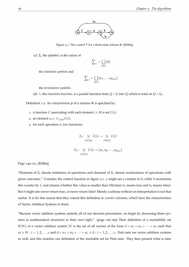
Figure 3.1: The control T for a finite-state schema Φ. [KM69]
(c) Σ, the alphabet, is the union ofÿ
i“
ď
aPA
tau
the initiation symbols andÿ
t“
ď
aPA
ta1, . . . , aKpaqu
the termination symbols.
(d) τ, the transition function, is a partial function from QˆΣ into Q which is total on QˆΣt.
Definition 1.2. An interpretation φ of a schema Φ is specified by:
1. a function C associating with each element i P M a set Cpiq;
2. an element c0 PŚ
iPM Cpiq;
3. for each operation a, two functions:
Fa :ą
iPDpaq
Cpiq Ñą
iPRpaq
Cpiq
Ga :ą
iPDpaq
Cpiq Ñ ta1, a2, . . . , aKpaqu
Page 149-151, [KM69].
“Elements of Σi denote initiations of operations and elements of Σt denote terminations of operations with
given outcomes.” Consider the control function in figure 3.1. a might set a counter to 0, while b increments
this counter by 1, and returns whether this value is smaller than 10(where b1 means true and b2 means false).
But b might also never return true, or never return false! Merely a schema without an interpretation is not that
useful. It is for this reason that they extend this definition to counter schemata, which have the characteristics
of Vector Addition Systems in them.
“Because vector addition systems underly all of our decision procedures, we begin by discussing these sys-
tems as mathematical structures in their own right.” (page 165-169) Their definition of a reachability set
RpWq of a vector addition system W is the set of all vectors of the form d ` w1 ` w2 ` ¨ ¨ ¨ ` ws such that
wi P W : i “ 1, 2, . . . , s and d` w1 ` w2 ` ¨ ¨ ¨ ` wi ě 0 : i “ 1, 2, . . . , s. Petri nets are vector addition systems
as well, and this matches our definition of the reachable set for Petri nets. They then present what is later

3.1. Parallel program schemata 17
known as a Karp&Miller tree, where they associate a rooted tree T pWq with a vector addition system W .
Note that no algorithm is given to construct this tree, it is simply described in rules:
• A rooted tree is a directed graph such that one vertex (the root δ) has no edges directed into it,
• each other vertex has exactly one edge directed into it,
• and each vertex is reachable from the root.
• If ζ and η are distinct vertices of a rooted tree, and there is a path from ζ to η, then we say ζ ă η;
• if there is an edge from ζ to η, then η is a successor of ζ.
• A vertex without successors is called an end.
• A labelling lpζq assigns to each vertex ζ an r-dimensional vector whose coordinates are elements of
NY tωu.
(1) The root is labelled d;
(2) Let η be a vertex;
(a) if, for some vertex ζ ă η, lpζq “ lpηq, then η is an end.
(b) otherwise, the successors of η are in one-to-one correspondence with the elements w P W such
that 0 ď lpηq ` w. Let the successor of η corresponding to w be denoted by ηw. For each i the ith
coordinate of the label lpηwq is determined as follows:
(i) if there exists ζ ă ηw such that lpζq ď lpηq `w and lpζqi ă plpηq `wqi then lpηwqi “ ω;
(ii) if no such ζ exists, then lpηwqi “ plpηq `wqi.
“We remark that, since T pWq is finite, its construction, using the recursive definition, is clearly
effective.”
It is then proven that this tree is always unique, finite, and can be used to solve a number of problems, like
the coverability problem, and whether coordinates can be simultaneously unbounded. It’s also shown that
Vector Addition Systems can be transformed into counter schemata without loss of behaviour, and vice versa:
Let pP, T, W, Mq be a Petri net. The memory locations are the places P, the operations a are the transitions T,
and they only have one outcome, success. Let Q contain the reachable set, and let q0 be the initial marking
M. Then M r a yM1 if and only if
• τ maps from pM, aq to M,
• τ maps from pM, a1q to M1,
• τ maps no other pair pM, a1q,
• Dpaq Ď Rpaq,
• Fa describes Wpa, iq and Wpi, aq,
• Ga maps to success in all cases.
The rest of the paper focuses on schemata and is outside of the scope of this thesis.

18 Chapter 3. The algorithms
3.2 The minimal coverability graph for Petri nets
by Alain Finkel [Fin91]
“We arc interested in algorithms which take a Petri net PN and a property π in input and answer automati-
cally, after a finite delay, whether or not PN satisfies π.”
The properties in question are those that can be decided by the Karp&Miller tree: “the Boundedness Problem
(BP), the Finite Reachability Tree Problem (FRTP), the Finite Reachability Set Problem (FRSP), the Quasi-
Liveness Problem (QLP) or the equivalent problem called the Coverability Problem (CP) and the Regularity
Problem (RP). . . . One of our aims here is to define a graph which permits to decide upon these five problems
while, at the same time, being faster to compute and taking less space than the Karp-Miller graph.”
We remark that their definition of a coverability set is the same as ours, as it “is a set CS of markings such
that: 1) it covers all the markings of the reachability set and 2) for each marking m1 in CS but not in the
reachability set, there is an infinite strictly increasing sequence of reachable markings tmnu converging to
m1”, where converging is equivalent to our definition of a limit.
The paper then explains the minimal coverability graph(MCG) and minimal coverability tree(MCT) proce-
dures. “There are four basic ideas for constructing the minimal coverability graph”, which has the same defini-
tion as our MCG.
• The first idea is to develop the Karp-Miller tree until we meet two markings m and m1 such that m ě m1,
instead of m “ m1.
• The second idea is to compact the previous reduced Karp-Miller tree during its development. We
continue a marking m1 if and only if m1 is incomparable with any computed markings. If m ă m1, s.t.
there is a path from m to m1, we compute a new marking m2 such that for every marking m, we have:
for every place p, if m1ppq ą mppq then m2ppq :“ ω else m2ppq :“ m1ppq. Let n be the highest node m
used, we change its label to m2 and we remove its subtree.
• The third idea consists of removing every subtree whose root is labelled by a marking m such that
m ă m2. The idea is this will not produce new markings, but this is later proven faulty.
• Finally, the fourth idea is first to identify two nodes which have the same label; and mostly to only keep
arcs pm, t, m1q such that the transition t is fireable from m and we reach the marking m1 exactly, i.e. we
discard the pumping transitions.
The MCT procedure uses these first three ideas to make a non-unique minimal coverability tree. The MCG first
removes arcs that are no longer representations of a transition firing to get the unique minimal coverability

3.2. The minimal coverability graph for Petri nets 19
forest, and then identifies nodes with each other to get the unique minimal coverability graph. The calculations
made by the MCT procedure seem solid at first. However, a decade later, it is proven wrong. A counterex-
ample to the algorithm is shown in Figure 3.5.
Figure 3.2: Original figures detailing the effect of MCT and MCG. [Fin91]
“ Definition 7.1. A coverability tree CT(PN) of a Petri net PN “ tP, T, W, Mu is a labelled directed
tree tN, L, Au where the set of nodes N is a coverability set of PN, L “ T and arcs pn, t, n1q of A
(with labelpnq “ m and labelpn1q “ m1q are of types (1) or (2) :
(1) if m r t ym1 then there is an arc pn, t, n1q P A;
(2) if m r t y · and if ( not ( m r t ym1) ) then there is an infinite sequence of finite sequences of
transitions ttxnu such that for every n ě 0, the sequence of transitions txn is fireable from m,
we reach a marking mn and the sequence tmnu converges to m1: m r txn ymnand lim mn “ m1.
Definition 7.2. A minimal coverability tree MCT(PN) of a Petri net PN, is a coverability tree such
that its set of nodes is the minimal coverability set. The unique minimal coverability forest of a Petri
net, MCF(PN), is obtained from a minimal coverability tree by removing all arcs of type (2).
Proposition 7.3.
1) There is not a unique minimal coverability tree.
2) There is a unique minimal coverability forest.
3) The minimal coverability tree procedure computes a minimal coverability tree.” [Fin91]
The five problems (FRTP, FRSP, BP, QLP, RP) are all decidable with the minimal coverability graph (Corollary
3.17 [Fin91]).

20 Chapter 3. The algorithms
Theorem 3.1. Let PN be a Petri net, MCG(PN) its minimal coverability graph and MCS(PN) its minimal
coverability set.
1) The reachability tree RT(PN) is infinite if and only if there is at least one circuit in MCG(PN).
2) The reachability set RS(PN) is infinite if and only if there is at least one symbol ω in MCG(PN).
3) A place p is not bounded if and only if there is at least one marking M P MCS(PN) such that Mppq “ ω
4) A transition t is quasi-live if and only if there is at least one marking M P MCS(PN) such that for every
place p, Mppq ą Vpp, tq.
5) The language L(PN) is regular if and only if every elementary circuit of MCG(PN) containing an infinite
marking is labelled by a sequence of transitions x P T` such that Dpp, xq ě 0 for every place p.
For completeness, here is the algorithm description from the paper.
procedure minimal coverability graph(PN: Petri net; var MCS: set of markings; var MCG: graph);* the result will be in MCG *
beginminimal coverability tree(PN; MCS; MCT);identify nodes having same label(MCT; MCG);* the procedure “identify nodes having same label(T: tree; G: graph)” transforms the tree T into a graph Gsuch that two nodes in T having the same label are identified in G *for every arc pm, t, m1q of MCG do* after having identify nodes with the same label, we confuse without ambiguity a node and its label *
if not p mpt ą m1 q then remove arcppm, t, m1q; MCG);* the procedure “remove arcppm, t, m1q; var G))” only removes the arc pm, t, m1q from G *
end;
Figure 3.3: Original description of the minimal coverability graph procedure.

3.2. The minimal coverability graph for Petri nets 21
procedure minimal coverability tree(PN: Petri net; var MCS: set of markings; var MCT: tree);* the result will be in MCT *var unprocessednodes, processednodes: set of nodes; n, n1, nl , n2: node; t: transition; ancestor: boolean;
beginunprocessednodes := create nodepr, M0q ; * M0 is the marking of root r *processednodes := H; * processednodes will be the minimal coverability set *while unprocessednodes ‰ H do
beginselect some node n P unprocessednodes;unprocessednodes := unprocessednodes - tnu;case n : [1..4] of * m is the marking of n and m1 is the marking of n1 *
1: there is a node n1 P processednodes such that m “ m1 :begin
processednodes := processednodes + tnu;exit; * exit of case *
end;2: there is a node nl P processednodes such that m ă m1 :
beginremove node(n; MCT);exit; * exit of case *
end;* the procedure “remove node(n: node; var T: tree)” removes the node n and the arc from thedirect ancestor of n to n, in the tree T *
3: there is a node n1 P processednodes such that m1 ă m :begin
m2 :“ m; ancestor := false;for all ancestors n1 of n such that m1 ă m do
for all places p such that m1ppq ă mppq do m2ppq :“ ω;if there is an ancestor n1 of n such that m1 ă m2 then
beginancestor := true;n1 := first node processed, on the path from the root to n such that m1 ă m2;m1 :“ m2;remove tree(n1; MCT); * the procedure “remove tree(n: node; var T: tree)” which removes the subtreewhose root is n in the tree T (note that we keep the root n) * remove from(processednodes+unprocessednodes) all nodes of tree(n1;MCT);unprocessednodes := unprocessednodes + tpn1u;
end;for every n1 P processednodes such that m1 ă m2 do
beginremove from(processednodes+unprocessednodes) all nodes of tree(n1;MCT);remove tree(n1; MCT);remove node(n1; MCT);
end;if ancestor = false then unprocessednodes := unprocessednodes + tnu;exit; * exit of case *
end;4: otherwise :
beginfor every transition t such that mptą m1 do
begincreate node+arcppn, t, n1q; MCT); * m1 is the marking of the new node n1 * * the procedure “create node+arcppn, t, n1q; T)” creates a new node n1 labelledby m1 and a new arc pn, t, n1q in the tree T * unprocessednodes := unprocessednodes + tn1u;
end;processednodes := processednodes + tnu;exit; * exit of case *
end;end; * end of case *unprocessednodes := maximal(unprocessednodes); * the function “maximal(S : set) : set” computes the set of nodes n such that every label(n) is maximal * MCS := label(n) ; n P processednodes ;
end;; * end of while *end;; * end of procedure *
Figure 3.4: Original description of the minimal coverability tree procedure.

22 Chapter 3. The algorithms
3.3 On the efficient computation of the minimal coverability set of Petri
nets
by Gilles Geeraerts, Jean-Francois Raskin and Laurent Van Begin [GRB10]
This is one of the papers that proves the MCT algorithm to be wrong, as mentioned earlier. It gives us
a specific counterexample Petri net, and shows that the execution of MCT does not return the MCS. “The
flaw is intricate and we do not see an easy way to get rid of it.” The original images used to explain the
counterexample can be found in Figure 3.5. Instead of fixing this, they then show a new algorithm for
computing the MCS, focused on being correct rather than sacrificing correctness for speed. The experimental
results show that it behaves much better in practice than the KM algorithm.
“It is based on novel ideas: first, we do not build a tree but handle sets of pairs of markings.
Second, in order to exploit the monotonicity property, we define an adequate order on pairs of
markings that allows us to maintain sets of maximal pairs only. As a consequence, our new solution
manipulates sets that are minimal too (as the MCT intends to do), but for a different ordering (an
ordering on pairs, instead of an ordering on markings).”
“Given an ω-marking m of some PN N “ xP, Ty, we let Postpmq “ tm1|Dt P T : m r t ym1u and
Postpmq “ tm1|Dσ P T : m r σ ym1u.” The reachable set is thus PostpMq.
“Given a set M of ω-markings, we define the set of maximal elements of M as maxďpMq “
tm P M|Em1 P M : m ă m1u. Given an ω-marking m (ranging over set of places P), its downward-
closure is the set of markings Óďpmq “ tm1 P N|P||m1 ď mu. Given a set M of ω-markings, we let
ÓďpMq “Ť
mPM Óďpmq. A set D Ď N|P| is downward-closed iff ÓďpDq “ D.” Every set covers its
downward closure, and the downward closure of an ω-marking M is an infinite set that grows
arbitrarily large in places ΩpMq.
“Definition 4. Let N “ xP, Ty be a PN and let m0 be the initial ω-marking of N . The covering
set of N , denoted as CoverpN , m0q is the set ÓďpPost˚pm0qq. . . . a coverability set for N and m0 is
a finite sub-set S Ď pNY tωuq|P| such that ÓďpSq “ CoverpN , m0q.” The Cover is the downward
closure of the reachability set, equal to the downward closure of any coverability set.
“Given a set R of pairs of ω-markings, we let Flatten(R) = tm|Dm1 : pm1, mq P Ru. We use the
Post function to define the notion of successor of a pair of ω-markings (m1,m2): Postppm1, m2qq “
tpm1, m1q, pm2, m1q|m1 P Postpm2qu.” A pair pm1, m2q basically means that m2 is reachable from m1.
Any successor of m2 is reachable from both m1 and m2.
The acceleration in the K&M tree is called the function AccelpS, mq, where S are the ancestors
of m, and the return value is the new marking with added ω tokens. “Our new solution relies on

3.3. On the efficient computation of the minimal coverability set of Petri nets 23
Figure 3.5: Original figure with counterexample to MCT algorithm. [GRB10]A counter-example to the MCT algorithm. Underlined markings are in the frontier. A gray arrow from n ton1 means that n1 is the reason n was deactivated. Note how the execution returns an incorrect set. In step 3,
the marking tp3, ωp5u is deactivated, though no marking covering it is generated from tp2, p5u.

24 Chapter 3. The algorithms
a weaker acceleration function than that of Karp&Miller (because its first argument is restricted to
a single marking instead of a set of markings). Given two ω-markings m1 and m2 s.t. m1 ď m2,
we let AccelPairpm1, m2q “ mω s.t. for any place p, mωppq “ m1ppq if m1ppq “ m2ppq; mωppq “ ω
otherwise. Similarly to Post, we use Accel to define the notion of acceleration of a pair of ω-
markings pm1, m2q : Accelppm1, m2qq “ tpm2, AccelPairpm1, m2qqu if m1 ă m2; and Accelppm1, m2qq is
undefined otherwise. We extend the Post and Accel functions to sets R of pairs in the following
way: PostpRq “Ť
pm1,m2qPR Postppm1, m2qq and AccelpRq “Ť
pm1,m2qPR,m1ăm2tAccelpm1, m2qu.”
“Now that we have defined function to handle the semantics of the PN in terms of pairs, we
define the ordering Ď that will allow us to reduce the size of the sets our algorithm manipulate.
Let m1 and m2 be two ω-markings. Then, m1 a m2 is a function P ÞÑ ZY t´ω, ωu s.t. for any
place p : pm1 am2qppq is equal to ω if m1ppq “ ω;´ω if m2ppq “ ω and m1ppq ‰ ω; m1ppq ´m2ppq
otherwise. Then, given two pairs of ω-markings pm1, m2q and pm11, m12q, we have pm1, m2q Ď pm11, m12q
iff m1 ď m11, m2 ď m12 and for any place p : pm2 am1qppq ď pm12 am11qppq.” In other words, pair1 Ď
pair2 if pair1 is obsolete: pair1 has smaller markings with less growth. Remark that a never results
in ´ω, as xm1, m2y means that m2 is reachable from m1, and thus Ωpm1q Ď Ωpm2q.
“Example 11. Let us assume a PN with two places. Then: px0, 1y, x0, 2yq Ď px1, 1y, x2, 5yq and
px0, 1y, x0, 2yq Ď px1, ωy, x2, ωyq. However, px0, 1y, x0, 2yq Ę px1, 7y, x2, 7yq although x0, 1y ď x1, 7y and
x0, 2y ď x2, 7y. Indeed, x0, 2y a x0, 1y “ x0, 1y, x2, 7y a x1, 7y ´ x1, 0y and x0, 1y ę x1, 0y.”
Analogous to the Óďand Maxď on markings, we define ÓĎand MaxĎ on pairs: “For any pm1, m2q,
we let ÓĎppm1, m2qq “ tpm11, m12q|pm11, m12q Ď pm1, m2qu. We extend this to sets of pairs R as follows:
ÓĎpRq “Ť
pm1,m2qPR ÓĎppm1, m2qq. Given a set R of pairs of markings, we let MaxĎpRq “ tpm1, m2q P
R|Epm11, m12q P R : pm1, m2q ‰ pm11, m12q ^ pm1, m2q Ď pm11, m12qu.
“Definition 14. Given a Petri net N and an initial ω-marking m0, an oracle is a function Oracle
: N ÞÑ pNY tωuq|P| ˆ pNY tωuq|P| that returns, for any i ě 0, a set of pairs of ω-markings that
satisfies the two following conditions:
ÓďpPostpFlattenpOraclepiqqqq Ď ÓďpFlattenpOraclepiqqq
ÓďpFlattenpOraclepiqqq Ď CoverpN , m0q.2
In other words, each set FlattenpOraclepiqq is closed under Post, and does not contain any unreach-
able markings.
Now that we’re up to speed on the definitions this paper uses, we can get to the definition of their procedure
for calculating the MCS. “Definition 15. Let N “ xP, Ty be a PN, m0 be an initial marking, and Oracle be an
oracle. Then, the covering sequence of N , noted CovSeqpN , m0, Oracleq is the infinite sequence pVi, Fi, Oiqiě0,
defined as follows:

3.3. On the efficient computation of the minimal coverability set of Petri nets 25
• V0 “ H, O0 “ H and F0 “ tpm0, m0qu
• For any i ě 1 : Oi “ MaxĎpOi´1Y Oracle piqq;
• For any i ě 1 : Vi “ MaxĎpVi´1 Y Fi´1qz ÓĎpOiq;
• For any i ě 1 : Fi “ MaxĎpPostpFi´1q YAccelpFi´1qqz ÓĎpVi YOiq.
A covering sequence is thus a sequence of triples pVi, Fi, Oiq, for any i ě 0, where all the Vi, Fi and Oi are
sets of pairs of markings. Oi represents all the information provided by the oracle, Vi are the visited pairs,
that were once in the frontier Fi. “Remark that, in all these sets, only maximal (wrt to Ď) pairs are kept. This
allows to keep the size of these sets smaller.” They then continue to prove that
Theorem 27. LetN be a PN, m0 be its initial marking, Oracle be an oracle, and CovSeqpN , m0, Oracleq “
pVi, Fi, Oiqiě0. Then, there exists k ě 0 such that
(1) for all 1 ď i ă k :ÓďpFlatten pVi YOiqq ĂÓďpFlatten pVi`1 YOi`1qq;
(2) for all i ě k :ÓďpFlatten pVi YOiqq “ Cover pN , m0q.
In other words, after some amount of steps k the sequence stabilizes, and Vi YOi is the MCS. Building the
covering sequence in a bounded Petri net is comparable to building the K&M tree in a breadth-first-search
manner, as FlattenpFiq is equal to the set of nodes of the K&M tree at depth i.
This works for any Oracle. The empty Oracle, for which Oraclepiq “ H for all i ě 1, has correct results.
The Oracle can be used to feed information we have already gathered to the algorithm. Some subset of the
MCS, that is closed under Post, might already be known. This is used in the CoverProcpN , m0q algorithm,
which calculates the MCS of a Petri net N with initial marking m0. The oracle starts out empty. Whenever
an acceleration from m to m1 is encountered, the procedure recursively calls itself with CovProcpN , m1q. The
recursive call calculates the subset of the MCS that has ω tokens in at least locations Ωpm1q. At least, because
there are recursive calls every acceleration. Every call layer continues until it is stable, i.e.: the set ÓďpFlatten
pOi Y Viqq ĎÓďpFlatten pOi´1 Y Vi´1qq. The resulting Oi Y Vi are then passed on to the previous layer, and
used as an Oracle.
This approach mixes breadth-first-searching for an acceleration with depth-first exploring when an acceler-
ation is found. In only the deepest layers of the recursive call, the algorithm continues until a closed set of
visited pairs is found, and all layers above it quickly find that almost all their pairs are smaller (wrt Ď) than
the Oracle, stabilizing their own sequence.
The algorithm is shown in Figure 3.6, and an execution on the counterexample net is shown in Figure 3.7.
After iteration 6, the algorithm finds ÓďFlattenpO5 YV5q “ÓďFlattenpO6 YV6q and returns the MCS.
At the end of the paper are some results, comparing a K&M algorithm, a covering sequence with an empty
oracle, and CoverProc. It states that CovProc has a maximum of 4 pairs at a time during the kanban net,
pictured in B.4. Kanban starts out with three ω tokens, and the MCS is tω16u, so there are 13 accelerations.

26 Chapter 3. The algorithms
Figure 3.6: The CovProc algorithm [GRB10]
The maximum amount of pairs is calculated as maxt|Vi YOi Y Fi |, i ě 1u, but it only accounts for that layer.
The recursive calls of CovProc don’t count each other’s pairs. The K&M execution of kanban has way more
than ten thousand nodes, the execution stopped at 1222 seconds, more than the designated timeout period of
two minutes; filling the table was done inconsistently. Creating 16 nodes with a K&M algorithm takes more
time than generating 47 pairs(and thus 94 markings) in the CoverProc algorithm. There is also an entry for
the bounded readwrite net(B.1), with 11, 139 nodes in the K&M tree, taking 530 seconds, a factor 300 slower
than CovProc. This is in sharp contrast with my own findings in Section 5.3, where CovProc is a factor 2.5
slower than K&M.

3.4. Minimal coverability set for Petri nets: Karp and Miller algorithm with pruning 27
i Vi Fi
0 H pxp1y, xp1yq1 pxp1y, xp1yq pxp1y, xp2yq, pxp1y, xp6yq, pxp1y, xp7yq
2 pxp1y, xp1yq, pxp1y, xp2yq, pxp1y, xp6yq, pxp1y, xp7yqpxp1y, xp3yq, pxp2y, xp3yq, pxp1y, xp4, 2p5yq,pxp6y, xp4, 2p5yq, pxp1y, xp2, p5yq, pxp7y, xp2, p5yq
3pxp1y, xp1yq, pxp1y, xp2yq, pxp1y, xp6yq, pxp1y, xp7yqpxp1y, xp3yq, pxp2y, xp3yq, pxp1y, xp4, 2p5yq,pxp6y, xp4, 2p5yq, pxp1y, xp2, p5yq, pxp7y, xp2, p5yq
pxp1y, xp4yq, pxp3y, xp4yq, pxp2y, xp4yq,pxp1y, xp3, 3p5yq, pxp4, 2p5y, xp3, 3p5yq, pxp6y, xp3, 3p5yq,pxp1y, xp3, p5yq, pxp2, p5y, xp3, p5yq, pxp7y, xp3, p5yq
4
pxp1y, xp1yq, pxp1y, xp6yq, pxp1y, xp7yqpxp1y, xp3yq, pxp2y, xp3yq, pxp1y, xp4, 2p5yq,pxp6y, xp4, 2p5yq, pxp1y, xp2, p5yq, pxp7y, xp2, p5yq,pxp3y, xp4yq, pxp2y, xp4yq, pxp1y, xp3, 3p5yq,pxp4, 2p5y, xp3, 3p5yq, pxp6y, xp3, 3p5yq,pxp2, p5y, xp3, p5yq, pxp7y, xp3, p5yq
pxp3y, xp3, p5yq, pxp4y, xp3, p5yq, pxp2y, xp3, p5yq,pxp1y, xp4, 3p5yq, pxp3, 3p5y, xp4, 3p5yq,pxp4, 2p5y, xp4, 3p5yq, pxp6y, xp4, 3p5yq,pxp2, p5y, xp4, p5yq, pxp7y, xp4, p5yq
at this point, AccelpF4q accelerates the underlinedpairs to pump p5. CovProc(N, xp3, ωp5y) andCovProc(N, xp4, ωp5y) are called.
O5 is tpxp3, ωp5y, xp3, ωp5yq, pxp3, ωp5y, xp4, ωp5yq,pxp4, ωp5y, xp3, ωp5yq, pxp4, ωp5y, xp4, ωp5yqu
5
pxp1y, xp1yq, pxp1y, xp6yq, pxp1y, xp7yqpxp1y, xp4, 2p5yq, pxp6y, xp4, 2p5yq, pxp1y, xp2, p5yq,pxp7y, xp2, p5yq, pxp3y, xp4yq, pxp2y, xp4yq,pxp1y, xp3, 3p5yq, pxp4, 2p5y, xp3, 3p5yq,pxp6y, xp3, 3p5yq, pxp2, p5y, xp3, p5yq, pxp7y, xp3, p5yqpxp3y, xp3, p5yq, pxp4y, xp3, p5yq, pxp2y, xp3, p5yq,pxp1y, xp4, 3p5yq, pxp3, 3p5y, xp4, 3p5yq,pxp4, 2p5y, xp4, 3p5yq, pxp6y, xp4, 3p5yq,pxp2, p5y, xp4, p5yq, pxp7y, xp4, p5yq
pxp3, p5y, xp3, ωp5yq, pxp4, 3p5y, xp4, ωp5yq,pxp3, p5y, xp4, p5yq, pxp3, p5y, xp4, p5yq,pxp4y, xp4, p5yq, pxp2y, xp4, p5yq, pxp1y, xp3, 4p5yq,pxp4, 3p5y, xp3, 4p5yq, pxp3, 3p5y, xp3, 4p5yq,pxp4, 2p5y, xp3, 4p5yq, pxp6y, xp3, 4p5yq,pxp2, p5y, xp3, 2p5yq, pxp4, p5y, xp3, 2p5yq,pxp7y, xp3, 2p5yq
Figure 3.7: Table detailing execution of the CovProc algorithm on the counterexample to MCT.
3.4 Minimal coverability set for Petri nets: Karp and Miller algorithm
with pruning
by Pierre-Alain Reynier and Frederic Servais [RS13]
This paper introduces the Monotone-Pruning algorithm (MP), an improved K&M algorithm with pruning. The
pruning is not as agressive as in the MCT algorithm, but this allows the algorithm to be proven correct.
“The main difficulty is to prove the completeness of the algorithm, i.e. to show that the set returned by
the algorithm covers every reachable marking. To overcome this difficulty, we reduce the problem to the
correctness of the algorithm for a particular class of finite state systems, which we call widened Petri nets
(WPN). These are Petri nets whose semantics [is] widened w.r.t. a given marking m: as soon as the number
of tokens in a place p is greater than mppq, this value is replaced by ω.” The algorithm is proven to be
terminating and correct on WPN and standard Petri nets.
Their definition of a coverability set matches ours almost literally, as it is a set C of ω-markings such that:
“1) for every reachable marking m of N , there exists m1 P C such that m ď m1,
2) for every m1 P C, either m1 is reachable in N or there exists an infinite strictly increasing sequence of

28 Chapter 3. The algorithms
reachable markings pmnqnPN converging to m1.”
“The K&M Algorithm uses comparisons along the same branch to stop exploration (test of Line
5), that we call vertical pruning. We present in this section our algorithm which we call Monotone-
Pruning Algorithm as it includes a kind of horizontal pruning in addition to the vertical one. We
denote this algorithm by MP. It involves the acceleration function Acc used in the Karp and Miller
algorithm. However, it is applied in a slightly different manner.
Algorithm 2 Monotone Pruning Algorithm for Petri Nets.Require: A Petri net N “ pP, T, I, O, m0q.Ensure: A labelled tree C “ pX, x0, B, Λq and a set Act Ď X such that ΛpActq “ MCSpN q.
1: Let x0 be a new node such that Λpx0q “ m0;2: X :“ tx0u; Act :“ X; Wait :“ tpx0, tq | Λpx0q r t y ·u; B :“ H;3: while Wait ‰ H do4: Pop pn1, tq from Wait.5: if n1 P Act then6: m :“ PostpΛpn1q, tq;7: Let n be a new node such that Λpnq “ AccpΛpAncestorCpn1qXActq, mq;8: X :“ XY tnu; B :“ BY tpn1, t, nqu;9: if Λpnq ę ΛpAct) then
10: Act :“ Act z tx | Dy PAncestorCpxq s.t. Λpyq ď Λpnq ^ py P Act _y RAncestorCpnqqu;11: Act :“ Act Ytnu; Wait :“ Wait Ytpn, uq | Λpnq r u y ·u;12: end if13: end if14: end while15: Return C “ pX, x0, B, Λq and Act.”
“. . . nodes of the tree are partitioned into two subsets: active nodes, and inactive ones. Intuitively,active nodes will form the minimal coverability set of the Petri net, while inactive ones are kept toensure completeness of the algorithm.”
In this algorithm, AncestorC denotes the ancestors of a node, including itself. Act is always kept minimal this
way: if a node is covered by Act it will not pass line 9, and if a node greater than some active node n is found,
it will be removed in line 10 by x “ y “ n. Only active nodes need be used for acceleration, as any inactive
ancestors have been deactivated because a greater ancestor exists. Inactive nodes merely exist as candidates
for y in line 10, and even then only a subset of them needs to be kept:
Figure 3.8: Original figure detailing MP algorithm.

3.4. Minimal coverability set for Petri nets: Karp and Miller algorithm with pruning 29
On the left of Figure 3.8, if a node n is found such that another node is horizontally pruned, then that node
and all its descendants will not pass line 5. None of these nodes are in the MCS, nor will they be used for
accelerations, they can be discarded. On the right of Figure 3.8, if a node n is found greater than an ancestor
y of n, then all its descendants are removed in line 10. But in line 11, n is added to Act. Only the deactivated
nodes on the path from y to n are relevant, as they can still be used to deactivate n and its descendants.
Figure 3.9: Original figures detailing the difference between MCT and MP on the counterexample to MCT.
We can see that because of these mechanisms, the MP algorithm is able to handle the counterexample net
Ncex, as shown in Figure 3.9. In MCT, because node 6 is deactivated by node 7, it cannot be used by node 8
to deactivate node 7. Node 9 is then deactivated by node 7 as soon as it is discovered. This pitfall is avoided
by the MP, as deactivated nodes can be used to deactivate their descendants. When node n “ 8 is discovered,
Line 10 of the algorithm is used with x “ 7, y “ 6, and 7 is deactivated. Node 9 is now uncovered by Act,
and is not deactivated on discovery.
The order of the elements in Wait is not fixed, any element can be popped in Line 4. They prove that the
order does not matter for the correctness of the algorithm, so depth-first, breadth-first, or any order can be
used.
The algorithm is then proven correct, and compared to the K&M algorithm, the MCT aclgorithm, and the
CoverProc algorithm of the previous paper [GRB10]. The nets used to compare them are a subset of the
nets used in the previous paper as well. Two versions of the MP algorithm are used, a breadth-first and a
depth-first version.
The algorithms were implemented in Python, and compared in runtime and number of elements created.
Furthermore, the CoverProc algorithm wasn’t implemented, the data for its runtimes seem to be copied from
its paper. As there are several years inbetween these papers, they might have used inferior hardware for
computing these times, so it is ill-advised to draw conclusions from these numbers. However, as in my

30 Chapter 3. The algorithms
own results, CoverProc is several orders of magnitude slower than the MP algorithm, which itself has speed
similar to MCT, orders of magnitude faster than K&M. The BFS approach is overall slightly faster than the
DFS, but this is only significant in the bounded net “mesh2x2”.
In summary, the MP algorithm is fast, correct, and the order of exploration is completely free, allowing for
different exploration strategies. Indeed, in my own implementation, it uses the “most tokens first” approach
from the next paper.
3.5 Old and new algorithms for minimal coverability sets
by Antti Valmari and Henri Hansen [VH14]
The final paper we review introduces some new ideas. The reason previous algorithms were incorrect, or
why they required a lot of checking, was because they prune futures. If a marking covers an old one, not
only that marking but (a subset of) its descendants are deactivated as well. In this publication, a simpler
algorithm that lacks future pruning is presented and proven correct. It is demonstrated, using examples, that
neither approach is systematically better than the other.
This paper has a definition of MCS equivalent to ours: “Let M1, M2, . . . be ω-markings such that M1 ď M2 ď . . ..
Their limit is the ω-marking M “ limiÑ8
Mi such that for each p P P, either Mppq “ Mippq “ Mi`1ppq “ Mi`2ppq “
. . . for some i, or Mppq “ ω and Mippq grows without limit as i grows.” Note that ω tokens are allowed in the
markings Mi, as long as they are repeated in every Mi thereafter.
“Let M be a set of ω-markings. Then M is a limit of M if and only if there are M1 P M, M2 P M, . . . such that
M1 ď M2 ď . . . and M “ limiÑ8
Mi. . . . LetM be a set of markings andM1 a set of ω-markings. We define thatM1 is
a coverability set forM, if and only if
1. For every M PM, there is an M1 PM1 such that M ď M1.2. Each M1 PM1 is a limit ofM.
A coverability set is an antichain, if and only if it does not contain two ω-markings M1 and M2 such that M1 ă M2.
[. . . ] Each set M of markings has a coverability set that is an antichain. It is finite and unique. It consists of the
maximal elements of the limits ofM. [. . . ] Each set of markings has precisely one minimal coverability set.It is finite.
It is the antichain coverability set.”
Their algorithm is unnamed, and I will refer to it in later sections as the HanVal algorithm. The algorithm
tracks ALL found markings in a set F, the active markings in a set A, a workset of unprocessed pairs W, and
the tree itself, by assigning a back pointer M.B to every marking M. The set F is never trimmed, and exists

3.5. Old and new algorithms for minimal coverability sets 31
so no subtree is explored twice. F is implemented as a hashing table or similar data structure, so that it is
fast to test whether a marking has already been found. When pumping for ω tokens, in the “original KM
algorithm” all ancestors of M are compared to M, and add tokens to a marking M1, which then replaces the
label M in the tree. But ancestors might also be smaller than this marking M1! Thus, this algorithm uses
repeated history scanning in the Add-ω routine:
As shown in Figure 3.11, instead of pumping only p1 because p2, 1, 2q ą p1, 1, 2q, the result marking pω, 1, 2q
checks the history again. Because pω, 1, 2q ą p3, 1, 1q, p3 is pumped as well, so that the final result marking
is pω, 1, ωq. A notable difference with previous algorithms is that the ancestors used to pump need not be
active. While checking ancestors takes longer, the total amount of nodes can go down, as the pumping
sequence need not (partly) be fired again from the pumped node.
Another new technique used is history merging. Instead of a single back pointer M.B, there is a list of pointers.
If a marking M1 is encountered that is already in F, M is added to its back list. This requires some adjustments
in the Add-ω function, as all ancestors in what is now a subgraph above M1 must be compared to M1. An
example of how this is helpful is shown in Figure 3.12, as the new marking p0, 1, 1, 0q is now larger than two
of its predecessors, and can be pumped to p0, ω, ω, 0q.
The active set A is kept minimal, so that A is the MCS upon termination. Cover-checkpM1q checks if M1
is covered by any element in A, and if not, which elements of A are covered by M1. These elements are
then removed, and M1 is added to A. Any pairs in W whose first element was just removed from A is also
removed from W. Finally, the new marking is added to F, A, and all pairs pM1, tq are added to W.
This algorithm is proven to terminate and be correct for any order of elements of W. Instead of adding
tM1u ˆ T to W, the practical way is to let W simply be a set of markings, and to have each marking M have
the property M.next tr denoting the next transition to check. When a marking is removed from A, we can
now remove its “associated pairs” from W easily, by setting M.next tr to an end value.
The paper compares Breath-First Search(which has the added benefit of making W a queue), Depth-First
1 F :“ tMu; A :“ tMu; W :“ tMu ˆ T; M.B :“ nil2 while W ‰ H do3 pM, tq :“ any element of W; W :“ W z tpM, tqu4 if M r t y · then continue5 M1 :“ the ω-marking such that M r t yM1
6 if M1 P F then continue7 Add-ωpM, M1q
8 if ω was added then if M1 P F then continue9 Cover-checkpM1) // may update A and W
10 if M1 is covered then continue11 F :“ FY tM1u; A :“ AY tM1u; W :“ W Y ptM1u ˆ Tq;M’.B:“ M
Figure 3.10: The basic coverability set algorithm.

32 Chapter 3. The algorithms
Add-ω(M, M1)1 last := M; now :“ M; added := False2 repeat3 if now ă M1 ^ Dp P P : nowppq ă M1ppq ă ω then4 added := True; last := now5 for each p P P such that nowppq ă M1ppq ă ω do6 M1ppq :“ ω7 if now.B = nil then now := M else now := now.B8 until now = last
Figure 3.11: Original figures detailing repeated scanning of history.
Figure 3.12: Original figure detailing the advantage history merging.

3.5. Old and new algorithms for minimal coverability sets 33
Search(which makes W a stack), and the new Most Tokens First search. Most-tokens first sorts the markings
M by amount of ω tokens: |ΩpMq|, and then by amount of supply in the non-ω places:ř
pPΩpMq Mppq. This
greedy heuristic is based on the ideas that after pumping, the subtree at M1 will likely passivate a large
number of active markings, and should thus be explored first. Also, any pumping sequence will likely have
an increasing number of tokens in it, so those with most tokens are most likely to lead to pumping sequences.
“In our measurements (see Section 6), breadth-first was never clearly the fastest but was often clearly the
slowest. So we do not recommend breadth-first.” Instead, it is shown that using DFS or MTF with history
merging gives almost the same advantages as future pruning does:
“Theorem 3. Let the construction order be depth-first and history merging be applied. Assume that M0 r t1 ¨ ¨ ¨ tn yω Mn
and M0 ă M10. Assume that all transitions along the path M0 r t1 ¨ ¨ ¨ tn y
ω Mn were found before M10. After finding
M10, the algorithm will not fire transitions from Mn, unless M1
0 r t1 ¨ ¨ ¨ tn yMn.” [VH14]
Here, r t y ω denotes that accelerations may have happened after firing the transitions. An identical theorem
is given for most-tokens-first order. Intuitively, There is no need to passivate any descendants Mn of M0,
because they will be passivated once M1n|M1
0 r t1 ¨ ¨ ¨ tn yω M1
n is found. If Mn “ M1n, this passivation would
need to be undone as well. They conclude that future pruning is merely a nuisance for this algorithm. This
includes passivation/removal of nodes in a pumping cycle.
They specify this is one of the major reasons they suspect the HanVal algorithm to outperform the previous
MP-algorithm, as that one “requires checking whether the new ω-marking M strictly covers any element
in F (excluding the history of M). This is a disadvantage, because otherwise checking coverage against
A would suffice, A may be much smaller than F, and checking coverage is expensive.” In the basic MP-
algorithm, Figure 3.8, deactivated nodes are indeed kept in the tree C, and a naive approach of line 10 could
prove costly. However, further reading shows that in their implementation, only the deactivated nodes in a
pumping cycle are kept, while other deactivated nodes are removed entirely: A is hardly smaller than F.
An objective analysis of the HanVal algorithm follows, where they show two small Petri nets, and how either
DFS or MTF can outperform the other. On some slightly more standardized benchmarks “[MTF] was often
both the fastest and constructed the smallest number of ω-markings.”
Finally, they show some of their test results, as shown in Table 3.1. BFS, DFS and MTF were ran on six
benchmarks (fms, kanban, mesh2x, mesh3x2, multipoll[sic] and pncsacover) and shown is their total number
of constructed distinct ω-markings, that is, |F|. As transitions on markings are fired in order, they “ran each
experiment with transitions tried in the order that they were given in the input and in the opposite order”,
sometimes with a dramatic impact on the result. “This acts as a warning that numbers like the ones in the table
are much less reliable than we would like.” Next to these numbers are results from the MP-algorithm’s paper,
showing “number of elements passed in the waiting list”. The MP-algorithm however, is not only interested

34 Chapter 3. The algorithms
model |A| most tokens f. depth-first breadth-first [6]fms 24 63 53 110 56 421 139 809
kanban 1 12 12 12 12 12 12 114
mesh2x2 256 479 465 774 455 10733 2977 6241
mesh3x2 6400 11495 11485 8573 10394
multipoll 220 245 234 244 244 507 507 2004
pncsacover 80 215 246 284 325 7122 5804 1604
Table 3.1: Results from the paper.
in the MCS but also the tree created. As such, most elements of the MCS are the label of many different nodes.
It is unclear why these results are posted side-by-side, for they are useful for comparing neither memory use
nor runtime.
I was impressed by the heuristics used in MTF, and as the order of the workset is adjustable in the other
algorithms too, have incorporated it in the runtime-prioritizing variant of the algorithms.

Chapter 4
Theoretical analysis
While these algorithms all calculate the Minimal Coverability Set, there are some important differences
between the algorithms. The properties I will compare are:
• Correctness. Does the program calculate the MCS as claimed?
• Speed.
• Memory consumption.
• Amount of parallelism possible. A subjective measure, as I merely show the steps I did in my imple-
mentation.
• Firing Sequence detection. A major reason for calculating a SCG of a graph is to determine which firing
sequences are possible from the root. While unbounded nets yield an infinite number of possible firing
sequences, they can still be described by some form of expression. For example in Figure 2.4:
“p1, 0, ωq is reachable by σn “ pt1t2qn, as M r σn y Mn ě p1, 0, nq”. After calculating the elements of the
MCS, is it possible to construct a firing sequence for each element?
• Interconnectivity. The algorithms’ ability to show what elements of the MCS can reach each other. Is the
entire MCS reachable from any of its elements, can you split the MCS into components? If connected,
what is the sequence to get from configuration to configuration?
This last one is not as trivial as it seems, as shown in Figure 4.1. From the initial state, both t1 and t4 are
fireable, both leading to a marking covered by pω, ω, 0q. Firing t4 is a ‘dead end’ though, the interconnectivity
is not always clear from a shallow inspection of the MCS.
4.1 Karp and Miller
The original Karp&Miller algorithm [KM69] is very slow and uses a lot of memory, but it preserves a lot of
data. No node is ever edited after it is created, so this algorithm is very parallelizable, with a large read-only
tree shared between threads.
35

36 Chapter 4. Theoretical analysis
0, 0, 1start 0, 1, 0 3, 0, 0 ω, 1, 0 ω, ω, 0
1, 0, 0 ω, 0, 0
t1
t4
t2 t3 t3
t2t3t2, t3
Figure 4.1: A graph and its coverability graph.
By examining the arcs arc(n,t,n’) the algorithm stores, it is possible to construct all the fireable sequences
from any node in the graph, as there are many repeated subtrees. The sequence of any path from M to one
of its descendants M1 ě M can be fired arbitrarily many times from M. The interconnectivity is likewise
obvious, as there is a firing sequence leading from M to M1 iff there is a path in the tree from a node labeled
M to one labeled M1.
4.2 MCT/MCG
To combat the runtime and memory costs, the paper by Finkel [Fin91] suggests a modification of the K&M
algorithm “...to obtain an algorithm which directly computes the minimal coverability graph without computing the
whole Karp-Miller graph.” While the algorithm is fast and does not take much memory, it is not always correct,
and can rarely produce an error depending on the order the unfinished nodes are explored. [GRB10]
The MCT algorithm will not explore nodes if a marking covering that node has already been explored. This
covering node does not have to be an ancestor, but can be anywhere in the tree. Retroactively, any new node
added to the tree removes any nodes it covers, and their subtrees. If a node covers one of its ancestors, it
replaces it. With these modifications, we lose the relationship between arcs and firing a transition, with no
clear way to see either a sequence to get to a node nor which nodes can reach each other. The parallelism
takes a minor hit, as two comparable markings could be added to the workset at the same time, but this is

4.3. CoverProc 37
rectified by another check whether a covering element already exists.
4.3 CoverProc
The CoverProc algorithm [GRB10] uses pairs of markings pm1, m2q to indicate there is some sequence, possibly
including accelerations, to get from m1 to m2. The algorithm was devised with correctness in mind, and is the
largest and slowest of the non-K&M algorithms. No transitions are stored anywhere, so no firing sequence
detection.
The pairs are explored in a recursive algorithm, essentially a BFS. Sets of visited and frontier pairs are
generated inductively, and on each iteration their minimized, Flattened sets are compared, i.e. the set of only
the second markings in the pairs, with smaller markings removed. If this set doesn’t change in an iteration,
the algorithm is finished and returns the sets of visited pairs. Each separate set generation can be parallelized,
but the additional waiting and overhead has not shown any actual speedups in my tests.
Whenever an acceleration is found, the accelerated node is used as root in a recursive call to CoverProc, so it
is DFS wrt accelerations. The result of this recursive call is used in the layer before it as the oracle, removing
smaller pairs wrt the special Ď relationship. For any two pairs, p1 Ď p2 if the pairs in p2 are greater than
those in p1, and p2 has a greater growth (i.e., m2 ´m1) than p1.
Ideally, this should remove any pairs not needed for calculating the MCS, and prevent accelerations and
costly recursive calls. But the recursive call also stops when the Flattened set does not change, and returns
an “incomplete” set of pairs. Consider the net in Figure 4.2. We can immediately see that the MCS contains
the markings p1ωp3 and p2ωp3 and that these markings are reachable from each other. After firing t1t3t4,
the visited pairs contain pp1, p1 p3q, and a recursive call is started with p1ωp3 as root. After firing t3t4, the
recursive call ends, but it does not return pp2ωp3, p2ωp3q. As a result, the pair pp2, p2 p3q generated from
t2t4t3 is not covered (wrt Ď) and does a recursive call as well.
Figure 4.2: A bad net for CoverProc.

38 Chapter 4. Theoretical analysis
This also highlights the lack of interconnectivity. When an acceleration M ă M1 is found, only the pair
pM, Mωq is added to the visited pairs, but not any other pair pN, Mωq, even if M was reachable from N. In
the example, pp1, p1ωp3q exists, but neither pp4, p1ωp3q nor pp1, p2ωp3q do.
4.4 Monotone Pruning algorithm
Reynier and Servais had the approach of doing both horizontal and vertical pruning with the Monotone
Pruning Algorithm. It uses a visited set and a working set, which can contain active and inactive nodes.
Only active nodes can deactivate other nodes, preventing the deactivation loop that was possible in the MCT
algorithm. The algorithm is proven correct. The flexible part of the algorithm is the way to pick pairs pM, tq
from the working set. The paper compares BFS, DFS, and ‘most tokens first’ approaches, considering the last
one superior in most cases. Whichever way chosen, the speed is comparable or superior to the speed of MCT,
with minimal memory cost. It is also easy to run in parallel, as the only side effect of the race condition is
too many nodes in the active set, which does not interfere with the correctness. Transitions are stored in the
tree, and nodes used in an acceleration are deactivated, not removed, so the accelerating sequence is visible
as well.
Interconnectivity is not readily visible from the tree. Let M r t y N r . . . y N1, and M1 r t1 y N. Naturally, N1
is also reachable from M1, but when the second node labelled N is found, a marking equal to it (and thus
covering it) has already been found, and it is deactivated. If we transform the tree into a reachability graph
by identifying nodes with the same label, the path from M1 to N1 emerges, and interconnectivity is as simple
as checking for existence of a path.
4.5 HanVal
Hansen and Valmari went a different way, pruning not more but less than MCT. The unnamed algorithm
(called HanVal by me) utilizes a working set, with pairs pM, tq of markings and transitions (possibly optimized
away in the implementation). It uses a pruning system prunes similar to MCT, but only deactivates nodes
when a covering node is being explored, not when it is discovered. The correctness is proven in the paper,
and its speed and memory are comparable to the MP algorithm. The algorithm is able to run in parallel quite
well, as the only critical part of the algorithm is Cover-check. Even that part can be run in parallel a bit, as it
is read-only if a covering marking is found.
The firing sequence detection is harder, because of history merging. Even when a back pointer would store
the transition used, the execution of Add-ω depends on the entire history of a node n at that moment. In the
final graph, this node can have ‘more’ history, if some node merged its history with an ancestor of n. The
good side of this is that interconnectivity is as easy as checking whether a path exists in the tree.

4.6. Summary 39
4.6 Summary
Name Correct Speed Memory Parallelizable Sequence detection Interconnectivity
K&M Y Slowest Most All Y Y
MCT Mostly Fast Little Mostly N N
CoverProc Y Slow Much Little Y N
MP Y Fast Least Mostly Y minor work
HanVal Y Fast Least Mostly N Y
While these criteria are sometimes important, the biggest factors are still execution time and memory cost. In
the next chapter we will compare implementations of the algorithms on some Petri nets for better compari-
son.

40 Chapter 4. Theoretical analysis

Chapter 5
Empirical evaluation
5.1 Program
Because theoretical investigation of the algorithms can only go so far, the only way to really compare the
algorithms is to implement them and use them on some Petri nets. To this end I implemented various
versions of each of the algorithms we have discussed so far. The algorithms were then tested on a series of
benchmarks, not just the most favorable Petri nets for each algorithm, as is usually done in the algorithms’
own presentations. Of these benchmarks, four are bounded nets, seven are unbounded.
The benchmarks used are described in Table 5.1, and the subsequent figures detail each algorithms’ execution
time. Tests were ran on more bounded nets, but execution times were less than a millisecond, even for
KarpMiller, so these nets were not useful for comparison. As a result of this benchmark set, we can also
speak of the number of accelerations in a net, as there are no mutually exclusive ω tokens such as in Figure 2.6.
The .spec files do not offer an insightful first-glance view of the nets, so there are images of the Petri nets in
Appendix B, made with the program PIPE1.
Unfortunately, most of these unbounded benchmarks do not actually have an unbounded Petri net graph,
but merely have an initial marking containing at least one ω token. This token is then multiplied through
the transitions, sometimes even resulting in an MCS of the sole marking ω|P|. Would these nets have a
standard initial marking, no ω token would ever come to be. Only one benchmark, “pncsacover”, has a
normal accelerating sequence: M r σ yM1 where M1 ą M and ΩM “ H.
Runtime and memory used are subjective factors, as they are influenced by both my specific implementation,
and the fact that the implementation language used, C#, is garbage collected instead of having exact memory
management. However, the amount of memory units taken, be it nodes, pairs or markings, is still an objective
measure of the algorithms’ effectiveness.
The program was executed on an Intel i5-2500K CPU at 3.3 GHz, 16GB RAM, running Windows 7 Home1http://pipe2.sourceforge.net/
41

42 Chapter 5. Empirical evaluation
Premium. The 32-bit version of the program was used, so that algorithms were stopped when their used
memory exceeded 4GB.
There are three versions of each algorithm: the Simple versions are just that, the algorithms implemented in
the most straightforward way. This includes implementing a @x P t. . .u as a for statement iterating that set,
when this may not be a good way to do it. The Simple versions keep all data, the complete trees, transition
names, etc., if the algorithm did that. There is the Speed versions, which focus on calculating the MCS. No
redundant data is stored, all data is thrown away as soon as it isn’t needed for the MCS. Most algorithms
use the most-tokens-first approach that Hansen and Valmari introduced, as the algorithms allow for any
order, and this MTF proved superior in early tests. Lastly there are Parallel versions. Most algorithms are
described as single-threaded programs, but even home computers have quad core CPUs. Most algorithms
were suited for a Worker approach, where several Worker threads(scaling to the amount of available cores)
execute the algorithm in parallel, with some care taken to avoid race conditions and incorrect executions.
Only CoverProc was not suited for this, which instead tries to calculate the new generation of sets in parallel
as much as possible. The HanVal algorithm does not have Simple and Speed, but DFS and MTF versions, to
compare my results to those in its paper.
The program is run as PetriTester <TestSize> [<timeoutms> [<Folder>]]. It will check the folder for
files ending in “.spec”, and tries to interpret them as Petri nets, or ‘benchmarks’. It runs the algorithms in
a random order on the benchmarks in a random order, until each combination has run TestSize amount of
times. It stores the results in the file “results.dat”. For each execution it stores the results:
• the amount of milliseconds taken
• the amount of ticks taken, a slightly more precise unit
• the amount of memory units in use at program termination
• the maximum amount of memory units in use at any time during execution
• the amount of elements in the calculated MCS
• the first 20 elements of the MCS
Subsequent program executions will sort the “results.dat” file to a more readable format if any algorithm
execution failed, and add result to the file if a greater TestSize was given. No previous results are erased.
• The main program is found in Program.cs. It builds a list of PetriNet objects that it reads from the .spec
files, and creates a list of Grapher objects that are the implementations. It then reads the “results.dat”
file for previous results, and runs the Grapher-PetriNet that aren’t found (enough). The combination
is run in a separate thread, so that it can timeout after 10 minutes (or the given timeout parameter). It
saves the results back into the “results.dat” file after each combination.
• The file Common.cs holds the common elements all algorithms share. The Grapher base class is described
here, requiring at least a Run method and a FinalMarkings property to be implemented by subclasses.
The algorithms are subclasses of Grapher.
The classes PetriNet, Transition and Marking are here as well.

5.2. Implementations 43
• DataStructures.cs holds the MTFHashSet, a set with fast operations for adding a marking and check-
ing existence, while still having a fast operation for retrieving the most-tokens marking. Also holds
ConcurrentMTFHashSet, which is thread-safe. Both of these use |P| ` 1 lists internally, each holding
markings with a different number of ω symbols, and each ordered by the supply in the non-ω places.
• FileHelper.cs and RunHelper.cs hold methods for reading files, saving results, and concurrent execu-
tion. The subfolders hold versions of the algorithms of that name.
The Benchmarks used are originally from the paper by Geeraerts, and can be found at their university’s
website.2 Most of them have also been used in the paper by Reynier and Servais, and in the paper by
Hansen and Valmari. The Petri nets used can have self-loops, as the transitions are described only as
“pplaces required for actionq Ñ peffect of actionq2. There is currently no support for actions that require a
specific range of supply in input places, nor for transfer or reset arcs. Adding additional benchmarks is as
simple as adding them to the folder, provided they follow the same syntax. Adding algorithms requires
changing the code, as they are implemented as Grapher objects. While it would be possible to implement
this as loading .dlls, this seemed too much work for a probably unused function.
5.2 Implementations
Most Simple versions use C#’s HashSet data structure, which allows for fast enumeration of the set, addition
and removal elements, and checking whether an element already exists. The elements are ordered by their
hash, resulting in a pseudo-random ordering of Markings, so that iterating the elements is not specifically
BFS nor DFS. Hashes are calculated only once each marking and are then memorized.
5.2.1 KarpMiller
The Karp&Miller [KM69] algorithm (A.2) retains all data about firing sequences, only checks for duplicate
markings in the ancestors of each node, and never trims or prunes in any way. Inefficient for bounded nets,
as this tree can have a height of |R| and a breadth ‘proportional to its concurrency’. It’s worse for unbounded
nets.
The Simple version iterates through the unfinished nodes by calling HashSet.First(), a pseudo-random
order based on the hashes for specific nodes. Nodes use the hash of their label, so adding an identically
labelled markings costs time linear to the amount of identically labelled markings already in the unfinished
nodes set. The Speed version goes for a DFS, as the order of exploration does not influence the resulting
tree. This has the advantage of lacking parent pointers: a node becomes a parent when explored, and stops
being one when this node is backtracked from. This is implemented with a Stack of markings, when a node
is done the next element can be popped from the stack. The Parallel version goes for BFS, as there are fewer
collisions between worker threads that way, and it’s not possible to omit parent pointers.2http://www.ulb.ac.be//di/ssd/ggeeraer/eec/

44 Chapter 5. Empirical evaluation
The benchmark multipool.
The Speed and Parallel version are only minimally faster than the Simple version, as it still has to compute
the entire tree. This is apparent on e.g. Petri net ‘multipool’ (Figure B.7): all four transitions t2, t5, t9 and
t11 lead to an acceleration immediately, but there are already 4! “ 24 different ways to do this, and any
combination of the other transitions can be fired before/after as well. The execution of Speed was stopped
after two hours, with no end in sight. All elements of the MCS had already been found because of the DFS
approach, but there was still an enormous tree to check.
5.2.2 MCT
The MCT [Fin91] algorithm (A.3) calculates the MCS with two separate procedures, simply named min-
imal coverability tree and minimal coverability graph. The Simple version keeps this structure, and iterates
through the unfinished nodes by pseudo-random Hashcode order. Nodes with already found markings
are still added to the tree, as is all transition information. After constructing the tree, it runs MCG to identify
equivalent Nodes.
The Speed and Parallel versions use the MTF order instead, and do not store any transition data. Furthermore,
no duplicate nodes are stored in the tree, so that it is not needed to identify them in MCG. This also allows
for faster coverage checking, as there are less Nodes to check against. However, no attempt was made to
combat the error, so the Parallel version is still quite prone to giving the wrong answer. Sometimes this rarely
happens, but on some nets this happens consistently.

5.2. Implementations 45
5.2.3 CovProcGraph
The CovProcGraph [GRB10] implementation (A.4) uses HashSets, where hashes of pairs are dependant on
both their markings, as no datastructure is fit for quick Ď checking. The only way to determine the maximum
elements in a set wrt. Ď is pairwise comparison of all of them, but we can use our knowledge of the sets for
some optimizations.
When determining Vi :“ MaxĎpVi1 Y Fi1qz ÓĎ pOiq, some elements need not be checked. Both Vi´1 had
elements covered by Oi´1 removed from them in the previous iteration, so if Oi is unchanged, this check
need not be made again. Likewise, Fi´1 does not need to compare elements with Oi if it is unchanged, but
still has to compare them to Vi.
When determining C “ maxĎpA Y Bq , where both sets A and B already contain maximal elements, then
@a P A, b P B : a Ď b implies:
• a R C
• b P C, because if there were an element a1 P A s.t. b Ď a1, then because the transitivity of Ď implies that
a Ď a1, conflicting with the maximality of A.
• There is no need to check for b1 ‰ b P B that b1 Ď a, because transitivity implies b1 Ď b, conflicting with
the maximality of B.
These considerations speed up the process of calculating maxĎ, but CovProc remains the slowest algorithm
by a landslide, apart from KarpMiller.
5.2.4 ReySer
The algorithm (A.3) by Reynier and Servais [RS13] does not impose an order in which the set of waiting nodes
should be processed, and compares a Depth First Search(DFS) and Breadth First Search(BFS) approach. The
Simple version uses a DFS order while the Speed version uses MTF, and the Parallel version uses MTF as
well. In every version, the algorithm is still:
1. Initialize active and waiting set with pairs of initial node M and every transition t.
2. Pop a pair pM, tq from the waiting set, or quit if there is none.
3. If t is not fireable jump to 2.
4. Fire t from M to obtain M1, then accelerate it to M2 by using the ancestors of M1. If any active node
covers M2, jump to 2.
5. Remove from active and waiting those nodes for which there is an ancestor(including the node itself)
that is covered by M2 and is either active or is NOT an ancestor of M1. Add M2 to active and pM2, tq to
wait for every transition t. Jump to 2.

46 Chapter 5. Empirical evaluation
The Speed/Parallel version use an enhanced version of this line:
10: Act :“ Act ztx | Dy P AncestorCpxq s.t. Λpyq ď Λpnq ^ py P Act _y R AncestorCpnqqu.
With a naive approach, this could cause a lot of useless checking, as any node is checked as candidate y for
every one of its descendants x. Instead, all nodes n are checked for being a possible y once, and those that
match are removed, with all their descendants.
5.2.5 HanVal
The unnamed algorithm (A.6) by Hansen and Valmari [VH14] returns to a K&M-like algorithm without any
pruning. The speed gain is gotten by merging nodes on discovery along with their history, and repeated
history scanning for faster accelerations. All markings found are stored in a hash-using Dictionary which
allows for fast adding of an unfound node, or adding to its history if it already exists.
5.2.6 Summary
The CovProcGraph algorithm [GRB10] shows promising results for some unbounded nets, but has abysmal
performance on the bounded nets. It was the only algorithm besides the KarpMiller algorithm to hit the
memory cap.
5.3 Results
The graphs show the amount of time taken, both in milliseconds and clock ticks, with about 3250 ticks per
millisecond. The data was generated by running all combinations twenty times and averaging the results,
with a timeout of one hour(timeout was 10 minutes in the meshx2 nets). In case of Parallel versions, some
outliers (probably due to delayed thread garbage collecting) were removed to get a better view of the time
spent computing. Both the millisecond and tick axis are logarithmic, but the scale is different with each
image, view with care.
In some cases, KarpMiller Simple seems to perform better than KarpMiller Speed/Parallel. This is because
the execution quickly fails because of lack of memory.
Bounded nets: As expected, the performance on bounded nets is quite similar for MCT, ReySer and HanVal.
They all simply explore the reachability graph of the net, while checking for accelerations. KarpMiller and
CoverProc took way longer, as they have each marking in their data structure multiple times.
Unbounded nets: To our disappointment, it seems that most of the benchmarks used by the researched papers
are hardly unbounded, that is: the transitions generate as much supply as they consume. The only reason
these nets are unbounded is because some places are initially unbounded, and these ω tokens propagate

5.3. Results 47
name |P| |T| |MCS| number of accelerations
lamport 11 9 14 bounded
newdekker 16 14 40 bounded
read-write 13 9 41 bounded
peterson 14 12 20 bounded
kanban 16 16 1 12
csm 14 13 16 3
fms 22 20 24 13
multipool 18 21 220 4
mesh2x2 32 32 256 12
mesh3x2 52 54 6400 20
pncsacover 31 36 80 11
Table 5.1: Benchmarks used.
throughout the net, even with “1:1 transitions”. Only the net ‘pncsacover’ was “truly unbounded”: it starts
without any ω tokens.
With these results, we can scrutinise the results of the analysed papers.
Geeraerts et al. compare their CovProc to the KarpMiller algorithm. [GRB10] Their results are questionable
at best, as even on bounded nets CovProc would outperform KM, though the amount of Nodes and Pairs
would suggest otherwise. The Petri net RTP (Figure B.3) only has markings consisting of a single supply. Yet
constructing the KM tree of 16 nodes would take more time than constructing the 47 pairs in the CovProc
algorithm. The net kanban (Figure B.4), is mistakenly shown as having a runtime longer than their timeout
period of 20 minutes. The KM tree does not have 9839 nodes, as my implementation gives an OOM error at
eight million nodes.
Not even the “Max Pairs” column of the CovProc algorithm is fair, as it seems to only count the amount of
pairs of a single layer: the recursive calls made to construct an Oracle count their pairs separately, as shown
by the kanban execution having a Max Pairs of just 4. This might also be why the runtime of the CovProc is
so low: My execution of KM on the net readwrite (Figure B.1) took 15 milliseconds, not seven minutes. My
execution of CovProc took 60 milliseconds, four times as much as the KM execution.
It is unknown whether this is a difference in measurement, or perhaps their implementation did not fol-
low their specification as strictly. In kanban, there are 10 different transitions used for acceleration, and
every different permutation of this order should lead to another recursive call, according to the line “Ri “Ť
mPSCovProcpN , mq where S Ď Flatten(AccelpFi´1qq”. No matter how complete the first return value is, the
other recursive calls are still made, in my implementation.
Reynier and Servais [RS13] copy these results to their own table, and justify this with “Note that the imple-
mentation of r7s also was in Python, and the tests were run on the same computer.” If this is true, then the KM

48 Chapter 5. Empirical evaluation
Figure 5.1: Execution results of lamport and newdekker.

5.3. Results 49
Figure 5.2: Execution results of read-write and peterson.

50 Chapter 5. Empirical evaluation
Figure 5.3: Execution results of kanban, csm and fms.

5.3. Results 51
Figure 5.4: Execution results of multipool.

52 Chapter 5. Empirical evaluation
Figure 5.5: Execution results of mesh2x2, mesh3x2 and pncsacover.

5.4. Summary 53
implementation used here and in [GRB10] vary wildly, as their K&M execution of readwrite took 6.33 sec-
onds, 60 times as fast. The ‘#Wait’ column is the total number of nodes in the tree, except for the kanban net,
which is said to have 72226 nodes with a runtime of just 9.1 seconds.
Nevertheless, the results for MP are different than mine as well. mesh2x2 (Figure B.8) takes about as long
(Simple is DFS), but multipool is done in 5ms instead of 5.2 seconds.
Lastly, Hansen and Valmari [VH12] do not compare runtimes, but “the total numbers of constructed distinct
ω-markings”. But that is what this algorithm specializes in, at the expense of different checking. It compares
this to the ‘#Wait’ column of the previous paper, which is the “number of elements passed in the waiting list”. An
element being a tuple pM, tq, but in HanVal “each ω-marking has an integer attribute next tr containing a number
of a transition”, and deactivation “is done simply by assigning to [the removed marking].next tr a number that is
greater than the number of any transition”. HanVal has this number optimised but MP hasn’t.
5.4 Summary
Earlier results are all based on the strong points of the newest algorithm, and comparisons are done against
outdated and unoptimised results.
On bounded nets, there is hardly any difference. The MCT algorithm is just as effective, as its error is not
encountered in bounded nets. MP and HanVal perform similarly; the same set of nodes is built, there are just
different checks for acceleration and termination. Any differences in runtime are mere fractions of a second,
and the overhead takes the longest amount of computation.
Space complexity is not an issue. Apart from KarpMiller and CovProc, the maximum memory used is often
not even 10% above the size of the MCS.
What’s also clear is that runtime is hardly ever an issue in the nets used. Only KarpMiller and CovProc
struggle with some of them, both in time and space complexity. But the other algorithms usually run in
under a millisecond, even the mesh3x2 net runs in under a minute. The clear winner is the MP algorithm in
MTF order, as it is the fastest in all unbounded nets. Hansen and Valmari had a useful contribution to all the
Speed versions with their MTF order. For any future comparisons to be useful, more complex Petri nets to
test on will be needed.
Lastly, parallelisation is rarely a good idea, dependant on the net. Multithreading on smaller levels like
checking ancestors might be more efficient, but is out of the scope of this thesis. Any subsequent accelerations
while using MTF order basically means the worker threads are useless, only the workers that have the current
maximum of ω tokens are being useful. If there are many accelerations like in kanban, parallelisation is
merely extra overhead. It is useful for exploring the ‘bounded component’ of markings reachable from the
same ω-marking M if M is in the MCS.

54 Chapter 5. Empirical evaluation

Chapter 6
Conclusions
We have reviewed several prominent papers in Chapter 3, containing algorithms for calculating the Minimal
Coverability Set. The heuristics used vary between not pruning at all, to pruning a lot more than the Ur-
algorithm MCG [Fin91]. Chapter 4 highlights some extra properties that can be derived from the results of
the algorithms, like sequence detection. This can be useful when interested in answering specific problems
as fast as possible, but does not matter if we are only interested in the MCS, in which case only memory
consumption and runtime matter.
Analytical evaluation is not useful, as it is possible to construct specific nets so that any algorithm seems
the superior one, as shown in the paper by Hansen and Valmari [VH12]. Only an evaluation of practical
performance is unbiased, if the benchmarks used are a good representation of the intended use of the algo-
rithms. Such an evaluation was done in Chapter 5. Earlier comparisons were also made in some papers, but
the results were often years apart, computed by different computers, or coded in a different language. Im-
plementations of the five algorithms were made in C#, and were run on several benchmarks, while tracking
their memory consumption and runtime. Graphs of the runtimes are shown in Section 5.3.
However, the predominant set of benchmarks is no longer as useful for comparison, as runtimes approach
mere milliseconds. Future testing of algorithms will mostly Memory is not an issue at all, as the set of
elements during runtime is barely larger than the MCS. A runtime comparison shows the Karp&Miller
algorithm and the CoverProc algorithms as slowest, often hitting the timeout cap. The best algorithm found
was the Monotone-Pruning algorithm by Reynier and Servais, if it used the simple but effective Most-Tokens-
First order devised by Hansen and Valmari. The effect of the order is huge, as the Depth-First order is a
factor 100 slower, and the MTF version even beats the MCT algorithm in speed.
55

56 Chapter 6. Conclusions

Appendix A
Program Code Sample
The full code is available from my supervisor and will be downloadable at the Leiden University website as
well.
A.1 Program.cs
using System;
using System.Collections.Generic;
using System.Linq;
using System.Threading;
using System.Diagnostics; //Stopwatch
namespace PetriTester
class Program
enum Status Success, OutOfMemory, Canceled, Failure ;
static int TIMEOUTMS;
static void Main(string[] args)
if (args.Length == 0 || args.Length > 3)
Console.WriteLine("Incorrect number of arguments.");
Console.WriteLine("Usage: PetriTester <TestSize> [<timeoutms> [<Folder>]].");
Console.WriteLine("Default Folder is current location.");
Console.WriteLine("Default timeout is 10 minutes, use -1 to wait indefinitely.");
57

58 Appendix A. Program Code Sample
return;
int TESTSIZE = int.Parse(args[0]);
TIMEOUTMS = (args.Length >= 2 ? int.Parse(args[1]) : 60000);
FileHelper.Folder = (args.Length == 3 ? args[2] : @".\");
PetriNet[] TheBenchmarks;
try
TheBenchmarks = FileHelper.ReadBenchmarks();
catch (Exception e)
Console.WriteLine("Error reading benchmarks in Benchmarks folder: 0", e.Message);
throw;
Type[] TheGraphers = new Type[]
typeof(KarpMiller_Simple),
typeof(KarpMiller_Speed),
typeof(KarpMiller_Parallel),
typeof(MCT_Speed),
typeof(MCT_Simple),
typeof(MCT_Parallel),
typeof(CovProcGraph_Simple),
typeof(CovProcGraph_Speed),
typeof(CovProcGraph_Parallel),
typeof(ReySer_Simple),
typeof(ReySer_Speed),
typeof(ReySer_Parallel),
typeof(HanVal_DFS),
typeof(HanVal_MTF),
typeof(HanVal_Parallel),
;
SortedDictionary<string, List<Result>> results = FileHelper.LoadData();
if (results == null)

A.1. Program.cs 59
Console.WriteLine("No previous valid results.dat found.");
results = new SortedDictionary<string, List<Result>>();
else
Console.WriteLine("Found results.dat, rewriting it to be clearer...");
FileHelper.SaveData(results);
CancellationTokenSource cts = new CancellationTokenSource();
Dictionary<string, int> failedRuns = new Dictionary<string, int>();
for (int test = 0; test < TESTSIZE; test++)
foreach (PetriNet pn in TheBenchmarks.Randomized())
foreach (Type grapherType in TheGraphers.Randomized())
string key = pn.ToString() + ", " + grapherType.ToString().Split(’.’).Last();
List<Result> list;
if (results.TryGetValue(key, out list) && list.Count >= TESTSIZE)
continue;
GC.Collect();
GC.WaitForPendingFinalizers();
Grapher grapher = (Grapher)Activator.CreateInstance(grapherType);
grapher.Init(pn);
Status status; //for debugging
cts = new CancellationTokenSource(TIMEOUTMS);
cts.Token.Register(MessageAborting, false);
Stopwatch sw = Stopwatch.StartNew();
try
Console.Write("Executing benchmark 0 with grapher 1...", pn.ToString(),
grapher.ToString());
grapher.Run(cts.Token);
status = Status.Success;
Console.WriteLine("Execution of benchmark 0 with grapher 1 succeeded. ",
pn.ToString(), grapher.ToString());

60 Appendix A. Program Code Sample
catch (OperationCanceledException)
Console.WriteLine("Execution of benchmark 0 with grapher 1 timed out. ",
pn.ToString(), grapher.ToString());
status = Status.Canceled;
catch (OutOfMemoryException)
Console.WriteLine("Out of memory executing benchmark 0 with grapher 1.
", pn.ToString(), grapher.ToString());
status = Status.OutOfMemory;
#if !DEBUG
catch (Exception)
Console.WriteLine("Execution of benchmark 0 with grapher 1 FAILED.",
pn.ToString(), grapher.ToString());
status = Status.Failure;
if (failedRuns.ContainsKey(key))
failedRuns[key]++;
else
failedRuns.Add(key, 1);
#endif
sw.Stop();
cts.Dispose();
bool tryAgain = true;
Result result;
saveresult:
Console.Write("Creating Result...");
try
result = new Result(sw, grapher);
if (list != null)
list.Add(result);
else
results.Add(key, new List<Result> result );

A.1. Program.cs 61
FileHelper.SaveResult(key, result);
catch
if (tryAgain)
tryAgain = false;
Console.Write("Error while creating Result, retrying...");
GC.Collect();
goto saveresult;
Console.Write("Error while creating Result, giving up...");
return;
Console.WriteLine("Appended result to file.");
#if DEBUG
Console.WriteLine(result.Markings);
#endif
//foreach grapher
//foreach benchmark
//for testsize
if (failedRuns.Count == 0)
Console.WriteLine("No failed runs. Rewriting save data to be clearer..");
FileHelper.SaveData(results);
else
Console.WriteLine("Failed runs:");
foreach (var kvp in failedRuns)
Console.WriteLine("0 failed 1 time(s).", kvp.Key, kvp.Value);
Console.WriteLine("Press any key to exit.");
Console.ReadKey();
//Main
static void MessageAborting()
Console.Write("Execution took longer than 0, now aborting...", TIMEOUTMS);

62 Appendix A. Program Code Sample
//Program
//namespace
A.2 KarpMiller.cs
using System;
using System.Collections.Generic;
using System.Linq;
using System.Text;
using System.Threading;
namespace PetriTester
class KarpMiller_Speed : Grapher
//Karp and Miller did not define a procedure to generate the tree, as it was more about the
mathematics than the computation.
//Instead, "Let \eta(PN) be a tree associated with a Petri Net PN such that <some conditions>
hold."
HashSet<Marking> nodes;
protected override IEnumerable<Marking> GetFinalMarkings()
var rv = nodes.Minimize();
nodes.Clear();
return rv;
public override void Run(CancellationToken CancellationToken)
//This is a faster implementation of the Karp&Miller algorithm, which focuses on
calculating the MCS as fast as possible, other data is redundant.
//As there is no pruning whatsoever, we can construct the tree in whichever order we want.
//We have chosen for a DFS approach, as it is easier to track ancestors of the current
node that way.
//Instead of following parent pointers, there is simply a set of ancestors. Nodes are
added when explored, and removed when backtracked from.

A.2. KarpMiller.cs 63
//The nodes currently being explored can be put in a Stack, where backtracking is done by
popping from the stack.
//We still explore Markings we have already explored before, or the algorithm would change
too much.
//The amount of Memory taken is cut back significantly, the total runtime not at all.
Stack<int> transitionCount = new Stack<int>();
Stack<Marking> unfinishedMarkings = new Stack<Marking>();
HashSet<Marking> ancestors = new HashSet<Marking>(Marking.EqualityComparer);
nodes = new HashSet<Marking>();
Marking currentMarking = initialMarking;
ancestors.Add(currentMarking);
nodes.Add(currentMarking);
int currentTransition = 0;
while (true)//unfinishedMarkings.Count != 0)
CancellationToken.ThrowIfCancellationRequested();
if (currentTransition == transitions.Length)
//this marking is done
//if completely done
if (unfinishedMarkings.Count == 0)
return;
//else we move on to a sibling, so currentNode is not an ancestor anymore
ancestors.Remove(currentMarking);
currentTransition = transitionCount.Pop();
currentMarking = unfinishedMarkings.Pop();
else if (currentMarking.IsFireable(transitions[currentTransition]))
Marking newMarking = currentMarking.Fire(transitions[currentTransition]);
//pump marking
Marking pumpedMarking = new Marking(newMarking);
foreach (Marking ancestor in ancestors)

64 Appendix A. Program Code Sample
if (ancestor < newMarking)
pumpedMarking.Pump(ancestor);
if (ancestors.Add(pumpedMarking))
CurrentMemory++;
//explore current node later
unfinishedMarkings.Push(currentMarking);
transitionCount.Push(currentTransition + 1);
nodes.Add(pumpedMarking);
currentMarking = pumpedMarking;
currentTransition = 0;
else
currentTransition++;
//if fireable
else
currentTransition++;
//while true
//Run
//KarpMillerGraph

A.3. MCT.cs 65
A.3 MCT.cs
using System;
using System.Collections.Generic;
using System.Linq;
using System.Threading;
namespace PetriTester
//as described on page 229 in
//THE MINIMAL COVERABILITY GRAPH FOR PETRI NETS
//by Alain FINKEL
//This version will focus on generating the MCS. Arcs are deemed irrelevant,
//and instead of two separate procedures MCT and MCG, nodes are identified with each other as
soon as discovered.
class MCT_Speed : Grapher
//Version of MCS that is focused on producing the MCS as quickly as possible.
//It therefore has no Arc objects that store transitions,
//and Nodes are a subtype of Marking, so that Nodes are identified by their Marking.
//processedNodes and unprocessedNodes are now MTFHashSets that prioritize markings with a
large number of Omega tokens.
private MTFHashSet processedNodes;
private MTFHashSet unprocessedNodes;
protected override IEnumerable<Marking> GetFinalMarkings()
return processedNodes;
public class Node : Marking
public bool removed = false;
public Node parent = null;
public List<Node> children;
public Node(Marking m) : base(m)
children = new List<Node>();

66 Appendix A. Program Code Sample
public Node(Marking m, Node parent) : base(m)
this.parent = parent;
children = new List<Node>();
public new Node Fire(Transition t)
return new Node(supply.Add(t.effect));
public override void Run(CancellationToken CancellationToken)
#region original description
/*
* procedure minimal_coverability_graph(PN: Petri net; vat MCS: set of markings; vat MCG:
graph);
* the result will be in MCG *
begin
minimal_coverability_tree(PN; MCS; MCT);
identify_nodes_having_same_label(MCT; MCG);
* the procedure "identify_nodes_having_same_label(T: tree; G: graph)" transforms the
tree T into a graph G such that two nodes in T having the same label are
identified in G *
for every arc (m,t,m’) of MCG do
* after having identify nodes with the same label, we confuse without ambiguity a
node and its label *
if not ( m(t>m’ ) then remove_arc((m,t,n’); MCG);
* the procedure "romove_arc((m,t,m’); ear G))" only removes the arc (m,t,m’) from G *
end;
*
procedure minimal_coverability_tree(PN: Petri net; var MCS: set of markings; var MCT:
tree);
* the result will be in MCT *
var unprocessednodes, processednodes: set of nodes; n, n’, n1, n2: node; t:
transition; ancestor: boolean;
begin
unprocessednodes := create node(r,M_0) ; * M_0 is the marking of root r *
processednodes := \emptyset; * processednodes will be the minimal coverability set
*
while unprocessednodes \neq \emptyset do
begin

A.3. MCT.cs 67
select some node n \in unprocessednodes;
unprocessednodes := unprocessednodes - n;
case n : [1..4] of * m is the marking of n and m_1 is the marking of n_1 *
1: there is a node n_1 \in processednodes such that m = m_1 :
begin
processednodes := processednodes + n;
exit; * exit of case *
end;
* 2: there is a node n_1 \in processednodes such that m < m_1 :
begin
remove_node(n; MCT);
exit; * exit of case *
end;
* the procedure "remove__node(n: node; var T: tree)" removes the node n and
the arc from the
direct ancestor of n to n, in the tree T *
3: there is a node n_1 \in processednodes such that m_l < m :
begin
m_2 := m; ancestor := false;
for all ancestors n_1 of n such that m_1 < m do
for all places p such that m_1(p) < m(p) do m_2(p) := \omega;
if there is an ancestor n_1 of n such that m_1 < m_2 then
begin
ancestor := true;
n_1 := first node processed, on the path from the root to n such that
m_1 < m_2;
m_1 := m_2;
remove_tree(n_1; MCT);
* the procedure "remove_tree(n: node; var T: tree)" which removes the
subtree
whose root is n in the tree T (note that we keep the root n) *
remove from(processednodes+unprocessednodes) all nodes of tree(n_1 ;MCT);
unprocessednodes := unprocessednodes + n_1;
end;
else
unprocessednodes := unprocessednodes + n;
for every n_1 \in processednodes such that m_1 < m_2 do
begin
remove from(processednodes+unprocessednodes) all nodes of tree(n_1;MCT;
remove_tree(n_1; MCT;
remove_node(n_1; MCT);
end;

68 Appendix A. Program Code Sample
exit; * exit of case *
end;
4: otherwise :
begin
for every transition t such that m(t>m’ do
begin
create_node+arc((n,t,n’); MCT; * m’ is the marking of the new node n’
*
* the procedure "create_node+arc((n,t,n’); T)" creates a new node n’
labelled by m’
and a new arc (n,t,n’) in the tree T *
unprocessednodes := unprocessednodes + n’;
end;
processednodes := processednodes + n;
exit; * exit of case *
end;
end; * end of case *
unprocessednodes := maximal(unprocessednodes);
* the function "maximal(S : set) : set" computes the set of nodes n such that
every label(n) is maximal *
MCS := label(n) ; n \in processednodes ;
end; * end of while *
end; * end of procedure *
*/
#endregion original description
#region optimisations
/*
* 1. Keeping unprocessedNodes maximized every iteration only needs to check the new
elements.
* 2. Keeping multiple nodes with the same marking is useless, it would only get removed
in MCG
* 3. The node pushed in case 3 has a label that was just pumped: there is no comparable
element in processednodes.
* Just fall through to case 4 with this new node instead of pushing and popping it.
* 4. As the assumption is that the order shouldn’t matter for correctness(we know it does
though),
* use a Most-Tokens-First set to designate the next node to treat.
*/
#endregion
processedNodes = new MTFHashSet(numPlaces, Marking.EqualityComparer);

A.3. MCT.cs 69
unprocessedNodes = new MTFHashSet(numPlaces, Marking.EqualityComparer);
Node currentNode, newNode, firstAncestor;
List<Node> list;
unprocessedNodes.Add(new Node(initialMarking, null));
//parent.Add(initialMarking, null);
while (unprocessedNodes.Count != 0)
CancellationToken.ThrowIfCancellationRequested();
currentNode = (Node)unprocessedNodes.Pop();
//case 1 is obsolete, no node is in the tree twice
//case 2
if (processedNodes.NoSmallerThan(currentNode).Any(LargerThan(currentNode)))
//remove the node by removing the ’arc’ to it
currentNode.parent.children.Remove(currentNode);
continue;
//case 3
//check if any ancestors are smaller
Node pumpedNode = new Node(currentNode, null);
firstAncestor = null;
for (Node walker = currentNode.parent; walker != null; walker = walker.parent)
if (walker < currentNode)
firstAncestor = walker;
pumpedNode.Pump(walker);
else if (walker < pumpedNode)
firstAncestor = walker;
//if a pump has happened
if (firstAncestor != null)
processedNodes.Remove(firstAncestor);
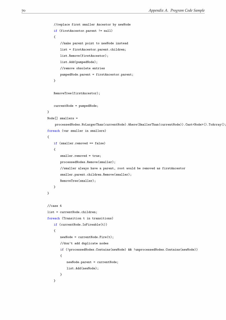
70 Appendix A. Program Code Sample
//replace first smaller Ancestor by newNode
if (firstAncestor.parent != null)
//make parent point to newNode instead
list = firstAncestor.parent.children;
list.Remove(firstAncestor);
list.Add(pumpedNode);
//remove obsolete entries
pumpedNode.parent = firstAncestor.parent;
RemoveTree(firstAncestor);
currentNode = pumpedNode;
Node[] smallers =
processedNodes.NoLargerThan(currentNode).Where(SmallerThan(currentNode)).Cast<Node>().ToArray();
foreach (var smaller in smallers)
if (smaller.removed == false)
smaller.removed = true;
processedNodes.Remove(smaller);
//smaller always have a parent, root would be removed as firstAncestor
smaller.parent.children.Remove(smaller);
RemoveTree(smaller);
//case 4
list = currentNode.children;
foreach (Transition t in transitions)
if (currentNode.IsFireable(t))
newNode = currentNode.Fire(t);
//don’t add duplicate nodes
if (!processedNodes.Contains(newNode) && !unprocessedNodes.Contains(newNode))
newNode.parent = currentNode;
list.Add(newNode);

A.3. MCT.cs 71
foreach (Marking m in list)
if (!unprocessedNodes.NoSmallerThan(m).Any(LargerThan(m)))
unprocessedNodes.Add(m);
//RemoveSmaller(m);
foreach (Marking rm in
unprocessedNodes.NoLargerThan(m).Where(SmallerThan(m)).ToArray())
unprocessedNodes.Remove(rm);
processedNodes.Add(currentNode);
CurrentMemory = processedNodes.Count + unprocessedNodes.Count;
//while unprocessednodes
//Run
/// <summary>
/// Removes the descendants of root from processedNodes and unprocessedNodes.
/// </summary>
/// <param name="removeMe"></param>
private void RemoveTree(Node root)
Stack<Node> removeThese = new Stack<Node>(root.children);
Node node;
while(removeThese.Count != 0)
node = removeThese.Pop();
if (processedNodes.Remove(node))
//remove its children too
foreach (Node n in node.children)
removeThese.Push(n);
node.children.Clear();
else
unprocessedNodes.Remove(node);
node.parent = null;

72 Appendix A. Program Code Sample
root.children.Clear();
Func<Marking, bool> LargerThan(Marking marking)
return (Marking m) => m > marking;
Func<Marking, bool> SmallerThan(Marking marking)
return (Marking m) => m < marking;
//KarpMillerGraph
A.4 CovProc.cs
using System;
using System.Collections.Generic;
using System.Linq;
using System.Threading;
namespace PetriTester
//as described in
//ON THE EFFICIENT COMPUTATION OF THE MINIMAL
//COVERABILITY SET OF PETRI NETS
//by GILLES GEERAERTS, JEAN-FRANCOIS RASKIN, LAURENT VAN BEGIN
//International Journal of Foundations of Computer Science(Oct 5, 2009)
class CovProcGraph_Speed : Grapher
HashSet<Pair> oracle;
HashSet<Pair> visited;
static CancellationToken CancellationToken;
class Pair : IEquatable<Pair>
public Marking m1;
public Marking m2;

A.4. CovProc.cs 73
bool hashed = false;
int hash;
public Pair(Marking m1, Marking m2)
this.m1 = m1;
this.m2 = m2;
public bool SquareSubset(Pair pair2)
return pair2.m1 >= this.m1 && pair2.m2 >= this.m2
&& pair2.m2 - pair2.m1 >= this.m2 - this.m1;
//pairs mean "you can get from m1 to m2", so m2 will have omega tokens at least at the
same places as m1.
//the minus here is well defined then
/// <summary>
/// Checks equality, first by reference, then by HashCode, then by contents.
/// </summary>
/// <param name="other"></param>
/// <returns></returns>
public bool Equals(Pair other)
if (ReferenceEquals(this, other))
return true;
return GetHashCode() == other.GetHashCode()
&& ReferenceEquals(this.m1, other.m1) || m1.EqualContents(other.m1)
&& ReferenceEquals(this.m2, other.m2) || m2.EqualContents(other.m2);
public override string ToString()
return string.Format("[0, 1]", m1 ,m2);
public override int GetHashCode()
if (!hashed)
unchecked
hash = (m1.GetHashCode() << 16) + (m1.GetHashCode() >> 16)
+ m2.GetHashCode();

74 Appendix A. Program Code Sample
hashed = true;
return hash;
public CovProcGraph_Speed()
CovProcGraph_Speed(CovProcGraph_Speed cpg, Marking marking)
numPlaces = cpg.numPlaces;
transitions = cpg.transitions;
initialMarking = marking;
override protected IEnumerable<Marking> GetFinalMarkings()
return Flatten(oracle.Concat(visited)).Minimize();
public override void Run(CancellationToken CancellationToken)
CovProcGraph_Speed.CancellationToken = CancellationToken;
RunInternal();
void RunInternal()
#if DEBUG
int iteration = 0;
#endif
//They’re all HashSets so that checks for duplicates can quickly be made. See the
MaxSquare functions.
oracle = new HashSet<Pair>();
visited = new HashSet<Pair>();
HashSet<Pair> frontier = new HashSet<Pair>();
HashSet<Pair> recursive = new HashSet<Pair>();
frontier.Add(new Pair(initialMarking, initialMarking));
Marking[] iterationCondition1;
Marking[] iterationCondition2 = new Marking[0];
bool oracleChanged = false;

A.4. CovProc.cs 75
do
CancellationToken.ThrowIfCancellationRequested();
#if DEBUG
iteration++;
#endif
iterationCondition1 = iterationCondition2;
foreach (Marking marking in Flatten(Accel(frontier)))
CovProcGraph_Speed cpg = new CovProcGraph_Speed(this, marking);
try
cpg.RunInternal();
finally
//record memory even when timed out
long temp = cpg.maxMemory;
CurrentMemory += temp;
CurrentMemory -= temp;
recursive = MaxSquarev2(recursive, Minimize(cpg.oracle.Concat(cpg.visited)));
if (recursive.Count != 0)
oracle = MaxSquarev2(recursive, oracle);
oracleChanged = true;
recursive.Clear();
//V_i:= Max ( V_i1 F_i1 ) \ (O_i);
//frontier_i-1 has already had its elements inferior to visited_i-1 removed
//frontier_i-1’s elements are already relevant wrt. visited_i-1
//we need to check if visited’s elements are still relevant wrt. frontier
visited.RemoveWhere(pair1 =>
frontier.Any(pair2 => pair1.SquareSubset(pair2)));
visited.UnionWith(frontier);
//if oracle hasn’t changed, then both frontier_i-1 and visited_i-1 are already maximal
wrt oracle, no need to check again
if (oracleChanged)

76 Appendix A. Program Code Sample
visited.RemoveWhere(pair1 =>
oracle.Any(pair2 => pair1.SquareSubset(pair2)));
//F_i:= Max (Post( F_i1 ) Accel( F_i1 )) \ (O_i V_i);
frontier = Minimize(Post(frontier)
.Concat(Accel(frontier)));
if (oracleChanged)
frontier.RemoveWhere(pair1 =>
oracle.Any(pair2 => pair1.SquareSubset(pair2)));
frontier.RemoveWhere(pair1 =>
visited.Any(pair2 => pair1.SquareSubset(pair2)));
CurrentMemory = oracle.Count + visited.Count + frontier.Count;
oracleChanged = false;
iterationCondition2 = Flatten(oracle.Concat(visited)).ToArray();
while (iterationCondition2.Any(m2 => //while there exists an object in flatten_i
!iterationCondition1.Any(m1 => m1 >= m2))); //not covered by any object in flatten_i-1
//Run
/// <summary>
/// Generates a List of new Pairs, based on firing transitions from the pairs in set. Does not
remove duplicates.
/// </summary>
/// <param name="set"></param>
/// <returns></returns>
List<Pair> Post(IEnumerable<Pair> set)
List<Pair> rv = new List<Pair>();
foreach (Pair pair in set)
rv.AddRange(Post(pair));
return rv;
IEnumerable<Pair> Post(Pair pair)
foreach (Marking m in Post(pair.m2))
yield return new Pair(pair.m1, m);
yield return new Pair(pair.m2, m);

A.4. CovProc.cs 77
IEnumerable<Marking> Post(Marking m)
foreach (Transition t in transitions)
if (m.IsFireable(t))
yield return m.Fire(t);
/// <summary>
/// Generates a List of new Pairs, based on possible accelerations within set. Does not remove
duplicates.
/// </summary>
/// <param name="set"></param>
/// <returns></returns>
List<Pair> Accel(IEnumerable<Pair> set)
List<Pair> rv = new List<Pair>();
foreach (Pair pair in set)
if (pair.m2 > pair.m1)
rv.Add(new Pair(pair.m2, AccelPair(pair)));
return rv;
Marking AccelPair(Pair pair)
Marking rv = new Marking(pair.m2);
rv.Pump(pair.m1);
return rv;
/// <summary>
/// Returns only the second elements of the pairs, removing duplicate markings.
/// </summary>
/// <param name="set"></param>
/// <returns></returns>
IEnumerable<Marking> Flatten(IEnumerable<Pair> set)
return set.Select(pair => pair.m2).Distinct(Marking.EqualityComparer);

78 Appendix A. Program Code Sample
HashSet<Pair> Minimize(IEnumerable<Pair> input)
return input.Aggregate(new HashSet<Pair>(), (set, pair1) =>
if (set.RemoveWhere(pair2 => !ReferenceEquals(pair1, pair2)
&& pair2.SquareSubset(pair1)) > 0
|| set.All(pair2 => ReferenceEquals(pair1, pair2)
|| !pair1.SquareSubset(pair2)))
set.Add(pair1);
return set;
);
/// <summary>
/// Returns the maximal elements(wrt the SquareSubset relation) of two already maximized sets.
/// </summary>
/// <param name="set1"></param>
/// <param name="set2"></param>
/// <returns></returns>
HashSet<Pair> MaxSquarev2(HashSet<Pair> set1, HashSet<Pair> set2)
if (set1.Count == 0)
return set2;
//Pairs in both sets are maximal in both sets, thus maximal in the union.
//Those elements can be returned, and no other elements need to be compared to them.
HashSet<Pair> rv = new HashSet<Pair>(set1.Intersect(set2));
set1.ExceptWith(rv);
set2.ExceptWith(rv);
//pairs can be approved or denied by a SquareSubset check
//if in one set, then not the other, as p1 <= p2 <= p1’ can not happen in maximized sets
//all pairs are unique, the intersection is already filtered
HashSet<Pair> approved = new HashSet<Pair>();
HashSet<Pair> denied = new HashSet<Pair>();
foreach (Pair pair1 in set1)
foreach (Pair pair2 in set2)
//check #1
if (!approved.Contains(pair1) && pair1.SquareSubset(pair2))

A.5. ReySer.cs 79
//pair1 is denied, pair 2 is approved
denied.Add(pair1);
approved.Add(pair2);
break; //no further checking is needed for this pair1
//check #2
if (!approved.Contains(pair2) && pair2.SquareSubset(pair1))
approved.Add(pair1); //keep checking, pair1 might be the single pair that
invalidates some pair2
denied.Add(pair2);
//for pair2 in set2
if (!denied.Contains(pair1))
rv.Add(pair1);
//don’t check denied elements in further iterations
set2.ExceptWith(denied);
denied.Clear();
//for pair1 in newSet1
//whatever wasn’t denied, and is thus still in set2, is a maximal element
rv.UnionWith(set2);
return rv;
//KarpMillerGraph
A.5 ReySer.cs
using System.Collections.Generic;
using System.Linq;
using System.Threading;
namespace PetriTester
//Faster version of the Monotone Pruning Algorithm.

80 Appendix A. Program Code Sample
//Uses a Most-Tokens-First approach to explore the set of unfinished nodes.
//Does not keep track of transitions, does not even remember the whole tree,
//What is remembered is a tree of active nodes, for each node, possibly a list of inactive nodes
associated with it.
//Optimized detection of covered nodes in lines 10/11.
class ReySer_Speed : Grapher
HashSet<Node> Act;
override protected IEnumerable<Marking> GetFinalMarkings()
return Act;
override public void Run(CancellationToken CancellationToken)
#region Original Description
//the Monotone Pruning Algorithm
//Algorithm 2 Monotone Pruning Algorithm for Petri Nets.
//Require: A Petri net N = (P, T, I, O, m0).
//Ensure: A labelled tree C = (X, x0, B, \Lambda) and a set Act X such that \Lambda(Act)
= MCS(N).
//1: Let x0 be a new node such that \Lambda(x0) = m0;
//2: X:= x0; Act:= X; Wait:= (x0, t) | Lambda(x0) \firet ; B:= ;
//3: while Wait \neq do
//4: Pop( n , t) from Wait.
//5: if n Act then
//6: m:= Post(Lambda( n ), t);
//7: Let n be a new node such that Lambda(n) = Acc(Lambda(Ancestor_C(n) Act),m);
//8: X:= X n; B:= B ( n , t, n);
//9: if Lambda(n) is not covered by anything in Lambda(Act) then
//10: Act:= Act \ x | y Ancestor_C(x) s.t. Lambda(y) Lambda(n) (y Act
y \not\in Ancestor_C(n));
//11: Act:= Act n; Wait:= Wait (n, u) | \Lambda(n) \fireu ;
//12: end if
//13: end if
//14: end while
//15: Return C = (X, x0, B, \Lambda) and Act.
// p P, Acc(M, m)(p) =: if m M | m < m m (p) < m(p) < ,
// =: m(p) otherwise.

A.5. ReySer.cs 81
#endregion
#region Optimizations
//**Original optimizations**
//In order to minimize the overhead of the inactive nodes, our implementation takes
advantage of the following observation.
//One of the following two cases occurs when a node x, different from the new node n, is
deactivated:
// if the new node n is not a descendant of x, then x and its subtree are completely
removed
// (indeed the algorithm will not need them anymore);
// if the new node n is a descendant of x an acceleration has occurred between n and an
ancestor y of x;
// the node x could be used later to deactivate one of the descendants of node n;
//in our implementation x
// is removed and the set of markings of the deactivated nodes lying between y and n
(including x)
// is associated with n; nevertheless, note that we only need to keep the minimal
elements of this set.
//Therefore our implementation maintains a tree data structure containing only the active
nodes and for
//each active node n it maintains the set of the minimal markings of the inactive
ancestors of n(up to the
//first active ancestor y of n).
//**endof original optimizations**
//**My optimizations**
//Identify a Node by its Marking, and check existence in Act(fast) before iterating
through all active nodes, when checking for coverage.
//10: Act:= Act \ x | y Ancestor_C(x) s.t. Lambda(y) Lambda(n) (y Act y
\not\in Ancestor_C(n));
//This is functionally equivalent to:
//"Remove from Act, all elements in x Act | Lambda(x) Lambda(n)
// ( y inactiveAncestors(x) s.t. Lambda(y) Lambda(n) x not Ancestor(n))
// and their descendants."
//i.e. look only for the top nodes.
//Of all nodes to remove, check which one is the highest ancestor of the active node,

82 Appendix A. Program Code Sample
//determine the path to the active node, and make those(and their own inactive sets) the
inactive set of the active node.
//Then remove all subtrees starting at such nodes.
//if n is deactivated, it is not in Act, popping it from Wait does nothing because of line
5.
//remove it from Wait, when deactivating
#endregion
Act = new HashSet<Node>(Marking.EqualityComparer);
MTFHashSet wait = new MTFHashSet(initialMarking.Length);
//1: Let x0 be a new node such that \Lambda(x0) = m0;
Node node = new Node(initialMarking);
//2: X:= x0; Act:= X; Wait:= (x0, t) | Lambda(x0) \firet ; B:= ;
Act.Add(node);
wait.Add(node);
//3: while Wait \neq do
while (wait.Count != 0)
CancellationToken.ThrowIfCancellationRequested();
//4: Pop( n , t) from Wait.
node = (Node)wait.First();
//5: if n Act then
while (node.IsActive)
int t = node.next_tr++;
if (t == transitions.Length)
wait.Remove(node);
break;
if (!node.IsFireable(transitions[t]))
continue;
//6: m:= Post(Lambda(n), t);
Marking original = node.Fire(transitions[t]);
//7: Let n be a new node such that Lambda(n) = Acc(Lambda(Ancestor_C(n) Act),m);

A.5. ReySer.cs 83
//8: X:= X n; B:= B ( n , t, n);
Node newNode = new Node(original);
var list = node.ActiveAncestors;
foreach (var ancestor in list)
if (ancestor < original)
newNode.Pump(ancestor);
//9: if Lambda(n) is not covered by anything in Lambda(Act) then
if (!Act.Contains(newNode) && !Act.Any(act => act >= newNode))
newNode.parent = node;
//10: Act:= Act \ x | y Ancestor_C(x) s.t. Lambda(y) Lambda(n) (y
Act y \not\in Ancestor_C(n));
//This is functionally equivalent to:
//"Remove from Act, all elements in x Act | Lambda(x) Lambda(n)
// ( y inactiveAncestors(x) s.t. Lambda(y) Lambda(n) x not
Ancestor(n))
// and their descendants."
Node[] removeThese = Act.Where(act => act <= newNode
|| (act.inactiveAncestors?.Any(anc => anc <= newNode) == true
&& !list.Contains(act)))
.ToArray();
//find highest removed ancestor
int index_top = list.Count - 1;
while (index_top >= 0 && !removeThese.Contains(list[index_top]))
index_top--;
//associate inactivated nodes with newNode
if (index_top != -1)
var top = list[index_top];
newNode.parent = top.parent;
top.parent?.children.Add(newNode);
top.parent?.children.Remove(top);
List<Node> path = list.Take(index_top + 1).ToList();

84 Appendix A. Program Code Sample
path.AddRange(path.Where(n => n.inactiveAncestors != null).SelectMany(n =>
n.inactiveAncestors).ToArray());
newNode.inactiveAncestors = Minimize(path, newNode);
else
if (node.children == null)
node.children = new List<Node>();
node.children.Add(newNode);
//remove the nodes and their descendants
Stack<Node> stack = new Stack<Node>(removeThese);
while (stack.Count != 0)
Node temp = stack.Pop();
if (temp.IsActive)
temp.IsActive = false;
Act.Remove(temp);
wait.Remove(temp);
if (temp.children != null)
foreach (Node child in temp.children)
stack.Push(child);
temp.children.Clear();
temp.inactiveAncestors?.Clear();
temp.parent = null;
//11: Act:= Act n; Wait:= Wait (n, u) | \Lambda(n) \fireu ;
Act.Add(newNode);
newNode.IsActive = true;
wait.Add(newNode);
CurrentMemory = Act.Count; //not counting associated inactive ancestors, there
can’t be many
break;
//endif newNode not covered by Act
//while node in Act

A.5. ReySer.cs 85
if (!node.IsActive)
wait.Remove(node);
//while Wait.Count != 0
//15: Return C = (X, x0, B, \Lambda) and Act.
return;
class Node : Marking
public Node parent;
public List<Node> children;
public List<Node> inactiveAncestors;
public bool IsActive = true; //A hashset is fast, a field is even faster
public int next_tr;
List<Node> m_ancestors;
List<Node> m_activeAncestors;
public Node(Marking label) : base(label)
public new Node Fire(Transition t)
return new Node(supply.Add(t.effect));
/// <summary>
/// Enumerates from self to root.
/// </summary>
/// <returns></returns>
public List<Node> Ancestors
get
if (m_ancestors == null)
m_ancestors = new List<Node>();
Node walker = this;
while (walker != null)
m_ancestors.Add(walker);
if (inactiveAncestors != null)
foreach (var inactive in inactiveAncestors)

86 Appendix A. Program Code Sample
m_ancestors.Add(inactive);
walker = walker.parent;
return m_ancestors;
/// <summary>
/// Enumerates from self to root.
/// </summary>
/// <returns></returns>
public List<Node> ActiveAncestors
get
if (m_activeAncestors == null)
m_activeAncestors = new List<Node>();
Node walker = this;
while (walker != null)
m_activeAncestors.Add(walker);
walker = walker.parent;
return m_activeAncestors;
//Node
List<Node> Minimize(List<Node> markings, Node anchor)
var temp = markings.ToList();
for (int i = temp.Count - 1; i >= 0; i--)
if (temp[i] < anchor
|| temp.Any(m => !ReferenceEquals(m, temp[i]) && m >= temp[i]))
temp.Remove(temp[i]);
return temp;

A.6. HanVal.cs 87
A.6 HanVal.cs
using System;
using System.Collections.Generic;
using System.Linq;
using System.Text;
using System.Threading;
namespace PetriTester
//This algorithm is defined on a rather low level.
//Making a _Simple version would at most change the way "W:= M0 x T" and the back pointers work.
//Thus, make a DFS and a MTF version instead, to mirror the results in the paper.
//The parallel version will parallelize the MTF version.
class HanVal_MTF: Grapher
class Node : Marking
public int next_tr = 0;
public new Node Fire(Transition t)
return new Node(supply.Add(t.effect));
public Node(Marking marking) : base(marking)
public Node(int?[] supply) : base(supply)
HashSet<Node> active;
Dictionary<Node, List<Node>> back;
override protected IEnumerable<Marking> GetFinalMarkings()
return active;
override public void Run(CancellationToken CancellationToken)

88 Appendix A. Program Code Sample
#region Original Description
/*
* 1 F := M0; A := M0; W := M0 T ; M0.B := nil
2 while W not= \emptyset do
3 (M,t) := any element of W; W := W \ (M,t)
4 if M .isfireable(t) then continue
5 M’ := the -marking such that M\fire(t)M’
6 if M’ F then continue
7 Add- (M,M’)
8 if was added then if M’ F then continue
9 Cover-check(M’) // may update A and W
10 if M’ is covered then continue
11 F := F M’; A := A M’; W := W (M’ T ); M’.B := M
*
* Add- (M,M’) //basic
1 last := M; now := M; added := False
2 repeat
3 if now < M’ p P : now(p) < M’(p) < then
4 added := True; last := now
5 for each p P such that now(p) < M’(p) < do
6 M’(p) :=
7 if now.B = nil then now := M else now := now.B
8 until now = last
*
* This is only the basic addOmega, add history merged scanning to it in our
implementation.
* Paper says something about a global search_now that is assigned to node.search_nr to
identify the last node used for pumping.
* I have no idea why you wouldn’t just compare a node’s pointer to the stored value of
this pointer.
* Let’s just do that. Or in C#, Node last = now. Exactly like in the code.
*/
#endregion
/*
* Merge histories if an identical marking is found, or covered by a marking that is
identical except for \omega tokens.
*
* PROOF OF CORRECTNESS
* Let M’ > M’’ in this specific way, having an \omega token where M’’ does not in places P’
* We would merge the history of M’’ with M’ to facilitate faster pumping. So let such a
pumping take place.

A.6. HanVal.cs 89
* Let N be an ancestor of M’’, N [\sigma> M’’, and M’ [\tau> N’ > N.
*
* Were we not to have merged, we would continue.
* Let D s.t. D(p) = 0 if N(p) = N’(p), D(p) = -\omega if N’(p) = \omega != N(p), and D(p)
= 1 otherwise.
* The effect of \sigma\tau is at least D.
* The effect of \tau\sigma is at least D.
*
* Note that D(p) = 1 in at least places P’.
* If M’’ does not have an \omega token, neither does N.
* If M’ has an \omega token, so does N’.
*
* N’ >= N, \sigma is fireable in N, so it is fireable in N’. Let N’[\sigma> M’’’
* M’[\tau\sigma> M’’’. M’’’ >= M’+ D. So pumping takes place in places P’.
* END OF PROOF
*
*/
//in short: KnM, no pruning, merged history and repeated history scanning.
//but it remembers found markings so as to not redo an explored subtree.
back = new Dictionary<Node, List<Node>>(Marking.EqualityComparer);
active = new HashSet<Node>();
MTFHashSet workingSet = new MTFHashSet(initialMarking.Length);
//1 F := M0; A := M0; W := M0 T ; M0.B := nil
Node node = new Node(initialMarking);
Node newNode;
List<Node> list;
back.Add(node, new List<Node>());
active.Add(node);
workingSet.Add(node);
CurrentMemory = 1;
//2 while W not= do
while (workingSet.Count != 0)
//3 (M, t) := any element of W; W:= W \ (M, t)
for (node = (Node)workingSet.Pop(); node.next_tr < transitions.Length; node.next_tr++)
CancellationToken.ThrowIfCancellationRequested();
Transition t = transitions[node.next_tr];

90 Appendix A. Program Code Sample
//4 if M .isfireable(t) then continue
if (!node.IsFireable(t))
continue;
//5 M’ := the -marking such that M\fire(t)M’
newNode = node.Fire(t);
//6 if M’ F then continue
if (back.TryGetValue(newNode, out list))
list.Add(node);
continue;
//7 Add- (M, M’)
if (AddOmega(node, newNode))
//8 if was added then if M’ F then continue
if (back.TryGetValue(newNode, out list))
list.Add(node);
continue;
//9 Cover - check(M’) // may update A and W
bool largerFound = false;
list = new List<Node>();
#region Cover-check(M’)
bool lesserFound = false;
foreach (Node act in active.ToArray())
if (!lesserFound)
int? result = Marking.Compare(newNode, act);
if (result != null)
if (result < 0) //newMarking < act
largerFound = true;
if (AlmostEqual(newNode, act))
back[act].Add(node);
continue;

A.6. HanVal.cs 91
if (result > 0) //newMarking > act
lesserFound = true;
if (AlmostEqual(act, newNode))
list.AddRange(back[act]);
active.Remove(act);
act.next_tr = transitions.Length;
else
//to check if act is strictly covered by marking is a smaller check than
comparing them completely
if (act < newNode)
if (AlmostEqual(act, newNode))
list.AddRange(back[act]);
active.Remove(act);
act.next_tr = transitions.Length;
//foreach act
#endregion
//10 if M’ is covered then continue
if (largerFound)
continue;
//11 F:= F M’; A := A M’; W:= W (M’ T ); M’.B := M
list.Add(node);
back.Add(newNode, list);
active.Add(newNode);
workingSet.Add(newNode);
CurrentMemory++;
//for transitions
//while WorkingSet not empty
//Run
bool AddOmega(Node root, Node newMarking)
//*add - (m, m’) //basic
//1 last:= m; now:= m; added:= false

92 Appendix A. Program Code Sample
//2 repeat
//3 if now < m’ p p : now(p) < m’(p) < then
//4 added:= true; last:= now
//5 for each p p such that now(p) < m’(p) < do
//6 m’(p) :=
//7 if now.b = nil then now := m else now:= now.b
//8 until now = last
//adapt this to back being a list of markings
//create ancestorset, removes duplicates
//this may seem overkill, but the ancestorset can be as big as the found set, so making a
distinct List in O(n^2) can be bad
HashSet<Node> ancestors = new HashSet<Node>();
Queue<Node> todo = new Queue<Node>();
Node current;
todo.Enqueue(root);
while (todo.Count != 0)
current = todo.Dequeue();
if (ancestors.Add(current))
foreach (Node parent in back[current])
todo.Enqueue(parent);
//loop through all ancestors until no change happened for an entire loop
Node last = ancestors.First();
bool added = false;
bool firstrun = true;
while (true)
foreach (Node now in ancestors)
if (!firstrun && now == last)
return added;
if (newMarking > now && newMarking.Pump(now))
added = true;
last = now;
firstrun = false;

A.6. HanVal.cs 93
//AddOmega
bool AlmostEqual(Node smaller, Node greater)
for (int i = 0; i < smaller.Length; i++)
if (greater[i] == null || greater[i] == smaller[i])
return false;
return true;

94 Appendix A. Program Code Sample

Appendix B
Benchmark images
Figure B.1: The Petri net read-write.
95
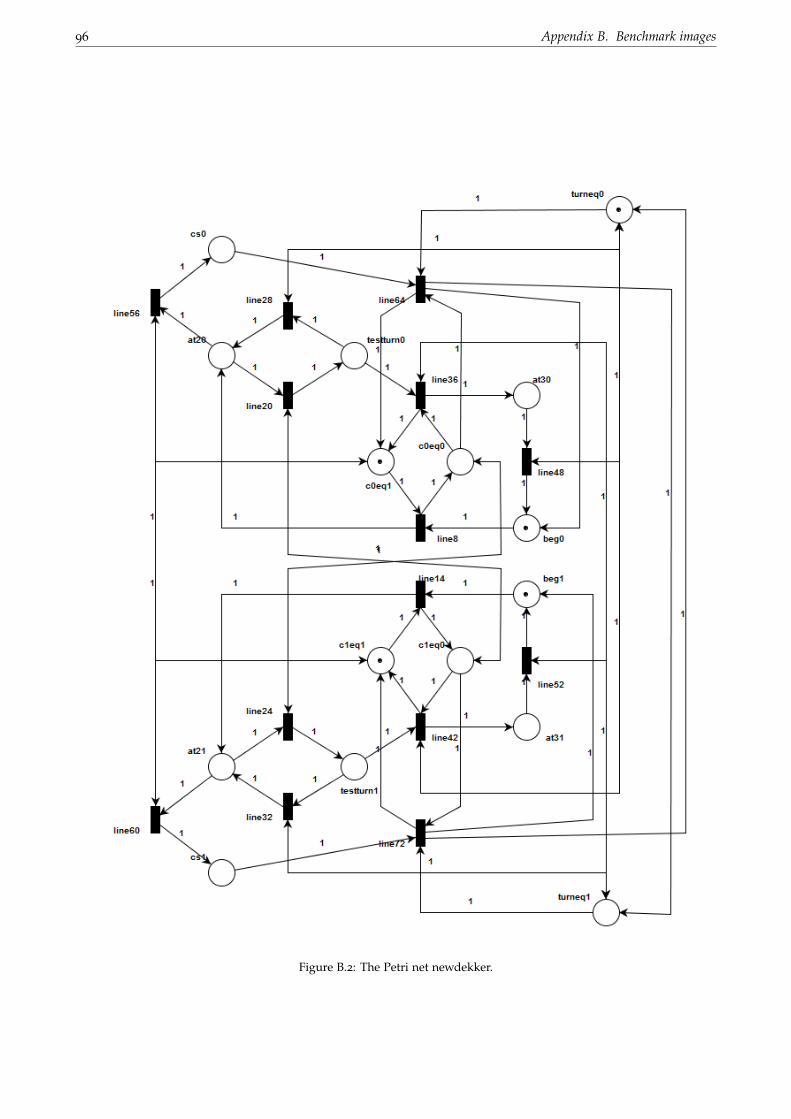
96 Appendix B. Benchmark images
Figure B.2: The Petri net newdekker.

97
Figure B.3: The Petri net newrtp.

98 Appendix B. Benchmark images
Figure B.4: The Petri net kanban.

99
Figure B.5: The Petri net csm.

100 Appendix B. Benchmark images
Figure B.6: The Petri net fms.

101
Figure B.7: The Petri net multipool.

102 Appendix B. Benchmark images
Figure B.8: The Petri net mesh2x2.

103
Figu
reB.
9:T
hePe
trin
etpn
csac
over
.Bol
ded
plac
esca
nge
tan
ωto
ken
duri
ngex
ecut
ion.

Bibliography
[AK76] Toshiro Araki and Tadao Kasami. Some decision problems related to the reachability problem for
petri nets. Theoretical Computer Science, 3(1):85 – 104, 1976.
[Bak73] Henry Baker. Rabin’s proof of the undecidability of the reachability set inclusion problem of vector
addition systems. 1973.
[BR09] Wilfried Brauer and Wolfgang Reisig. Carl adam petri and ”petri nets”. Fundamental Concepts in
Computer Science, 3:129–139, 2009.
[Dic13] Leonard Eugene Dickson. Finiteness of the odd perfect and primitive abundant numbers with n
distinct prime factors. American Journal of Mathematics, 35(4):413–422, 1913.
[Fin91] Alain Finkel. The minimal coverability graph for petri nets. In Advances in Petri Nets 1993, Papers
from the 12th International Conference on Applications and Theory of Petri Nets, Gjern, Denmark, June
1991, pages 210–243, 1991.
[GRB10] Gilles Geeraerts, Jean-Francois Raskin, and Laurent Van Begin. On the efficient computation of the
minimal coverability set of petri nets. Int. J. Found. Comput. Sci., 21(2):135–165, 2010.
[KM69] Richard M. Karp and Raymond E. Miller. Parallel program schemata. J. Comput. Syst. Sci., 3(2):147–
195, 1969.
[Reu90] Christophe Reutenauer. The Mathematics of Petri Nets. Prentice-Hall, Inc., Upper Saddle River, NJ,
USA, 1990.
[RS13] Pierre-Alain Reynier and Frederic Servais. Minimal coverability set for petri nets: Karp and miller
algorithm with pruning. Fundam. Inform., 122(1-2):1–30, 2013.
[VH12] Antti Valmari and Henri Hansen. Old and new algorithms for minimal coverability sets. In Appli-
cation and Theory of Petri Nets - 33rd International Conference, PETRI NETS 2012, Hamburg, Germany,
June 25-29, 2012. Proceedings, pages 208–227, 2012.
[VH14] Antti Valmari and Henri Hansen. Old and new algorithms for minimal coverability sets. Fundam.
Inform., 131(1):1–25, 2014.
104

BIBLIOGRAPHY 105
[VVN81] Rudiger Valk and Guy Vidal-Naquet. Petri nets and regular languages. Journal of Computer and
System Sciences, 23(3):299 – 325, 1981.


![Tele-Healthcare Computing and Engineering: …miodrag/papers/Wendt_telehealth...italizing on the energy savings gained using low data rates [35]. Each individual node’s data packet](https://img.pdfslide.net/doc/110x75/5f67772606e9db7474746c7d/tele-healthcare-computing-and-engineering-miodragpaperswendttelehealth-italizing.jpg)