Embed Size (px)
Citation preview

UNIVERSITI TEKNOLOGI MARA
A CASE STUDY ON RADIATE METHOD IN ON-LINE METHOD
IN CADASTRAL ADJUSTMENT
NUR ALIA BINTI AMIRUDIN
BSc
AUGUST 2020

UNIVERSITI TEKNOLOGI MARA
A CASE STUDY ON RADIATE METHOD IN ON-LINE METHOD
IN CADASTRAL ADJUSTMENT
NUR ALIA BINTI AMIRUDIN
Thesis submitted in fulfilment
Of the requirements for the degree of
Bachelor of Surveying, Science and Geomatics
(Hons)
Faculty of Architecture, Planning and Surveying
AUGUST 2020
i
CONFIRMATION BY PANELS OF EXAMINERS
I certify that the Panels of Examiners has met on 27 July 2020 to conduct the final
examination of Nur Alia Binti Amirudin on his Bachelor of Surveying Science and
Geomatics (Hons) thesis entitled “A Case Study on Radiation Method and On-Line
Method in Cadastral Adjustment” in accordance with Universiti Teknologi MARA Act
1976 (Akta 173). The Panels of Examiners recommends that the student be awarded
the relevant degree. The panel of Examiners was as follows:
Sr. Noorzalianee Ghazali
Faculty of Architecture, Planning and Surveying
Universiti Teknologi MARA
(Panel 1)
Sir Muhammad Faiz Bin Pa’Suya
Faculty of Architecture, Planning and Surveying
Universiti Teknologi MARA
(Panel 2)
Sr. Dr. Ashraf Bin Abdullah
Head,
Centre of Studies for Surveying
Sciences and Geomatics
Universiti Teknologi MARA,
Perlis Branch
Date: 27th JULY 2020
ii
AUTHOR’S DECLARATION
I declare that the work in this report was carried out in accordance with the regulations of
Universiti Teknologi MARA. It is original and is the result of my own work, unless
otherwise indicated or acknowledged a referenced work. This report has not been submitted
to any other academic institution or non-academic institution for any degree or
qualification.
I, hereby, acknowledge that I have been supplied with the Academic Rules and regulations
for Undergraduate, Universiti Teknologi MARA, regulating the conduct of my study.
Name of Student : NUR ALIA BINTI AMIRUDIN
Student I.D. No. : 2017801876
Programme : Bachelor of Science in Geomatics
Faculty : Architecture, Planning & Surveying
Thesis Title : A Case Study on Radiate Method in On-Line
Method in Least Square Adjustment
Environment
Signature of Student :
Date : 27th JULY 2020
iii
SUPERVISOR’S DECLARATION
“I hereby declare that I have read this industrial report and in my opinion this report is
sufficient in terms of scope and quality for the award of the Bachelor of Science Surveying
and Geomatics”.
Signature :
Name of Supervisor : Sr. NORSHAHRIZAN BIN MOHD HASHIM
Date : 27th JULY 2020
iv
ABSTRACT
Radiation method one of cadastral observation method where is suitable for locating
boundary marks which are within a single tape length (from the location of plane table)
and on-line method is a situation where a boundary marks are parallel towards other
boundary marks. This method usually performed during the land title of property
especially terrace house. However, there is an improvement when using these two
methods in terms of geometry data checking during field observations since LSA only
fulfil certain condition using these two methods. This paper highlight issues on how to
apply radiation method and on-line method in cadastral survey observation method. In
order to solve the aim of this study, there are three objectives need to be achieved which
is to study the variations of impact when performing radiation in on-line method and
to propose the new standard procedure relating to the issue given. The result of this
study will be a new guideline for radiate method in on-line method and to find the
suitability of using these two methods.

v
ACKNOWLEDGEMENT
Firstly, I wish to thank God for giving me the opportunity to embark on my degree and
for completing this long and challenging journey successfully. My gratitude and thanks
go to my supervisor Sr Norshahrizan Mohd Hashim, and co-supervisor, Sr Mohamad Asrul
Mustafar . Thank you for the support, patience and ideas in assisting me with this
project. I also would like to express my gratitude to the Department of Survey and Mapping
Malaysia providing the facilities, knowledge and assistance.
My appreciation special thanks to my colleagues and friends
for helping me with this project.
Finally, this thesis is dedicated to the loving memory of my very dear father and mother
for the vision and determination to educate me. This piece of victory is dedicated to both
of you. Alhamdulilah.
vi
TABLE OF CONTENTS
CONFIRMATION BY PANELS OF EXAMINERS .......................................................... i
AUTHOR’S DECLARATION ........................................................................................... ii
SUPERVISOR’S DECLARATION .................................................................................. iii
ABSTRACT ....................................................................................................................... iv
ACKNOWLEDGEMENT .................................................................................................. v
CHAPTER ONE INTRODUCTION ............................................................................... 1
1.1 Introduction 1
1.2 Research Background 1
1.2.1 Radiation Method 1
1.2.2 On-Line Method 2
1.2.4 Intersection Method 2
1.2.3 Bowditch Adjustment 3
1.3 Problem Statement 3
1.4 Aim and Objectives 4
1.5 Research Question 4
1.6 Scope and Limitation of Research 5
1.6.1 Scope of Work 5
1.6.2 Limitations and Challenges of Research 5
1.7 Significance of Study 5
1.8 Chapter Outline 6
CHAPTER TWO LITERATURE REVIEW ................................................................. 21
2.1 Introduction 21
2.2 Cadastral Survey 21
2.3 Observation Method in Bowditch Environment 21
2.3.1 Traverse Method 21
2.3.2 Double Independent Check (DIC) 22

vii
2.4 Observation Method in Least Square Adjustment Environment 22
2.4.1 Traverse Method 22
2.4.2 Radiate 22
2.4.3 Intersection 24
2.4.4 Resection 25
2.4.5 Global Navigation Satellite System (GNSS) 26
2.5 e-Cadastre 28
2.5.1 Coordinated Cadastral System (CCS) 29
2.5.2 National Digital Cadastre Database (NDCDB) 31
2.6 Online Observation 32
2.7 Issues of method observation during on-line observation in Least Square
Adjustment 33
2.7.1 Intersection 33
2.7.2 Resection 34
2.7.3 Radiate 34
2.8 Conclusion 34
CHAPTER THREE METHODOLOGY ........................................................................ 36
3.1 Introduction 36
3.2 Preliminary Studies 36
3.2.1 Data acquisition 36
3.2.2 Software used 37
3.3 Flowchart of methodology 39
3.4 Design of simulation data 42
3.5 Data Processing 46
3.5.1 Least Square Adjustment 46
3.5.2 Calculation of residual value 47
3.5.3 IBM SPSS Statistic 48
3.6 Result and Analysis 48
viii
3.7 Summary 48
CHAPTER FOUR RESULT AND ANALYSIS ........................................................... 50
4.1 Introduction 50
4.2 Result 50
4.2.1 Residual bearing, distance and area of radiate method 50
4.2.2 Double Independence Check (DIC) 64
4.2.3 Intersection 66
4.3 Analysis and Discussion 68
4.3.1 Residual bearing, distance and area of radiate method 68
4.3.2 Double Independence Check (DIC) Analysis 72
4.3.3 Intersection Method Analysis 73
CHAPTER FIVE CONCLUSION ................................................................................. 75
ix
LIST OF FIGURES
Figure Title Page
Figure 1.1 Radiation method............................................................................................... 1
Figure 1.2 Online method ................................................................................................... 2
Figure 2.1 Condition for radiate in closed traverse........................................................... 23
Figure 2.2 Radiate for open traverse ................................................................................. 24
Figure 2.3 Intersection method ......................................................................................... 25
Figure 2.4 Resection method procedure ........................................................................... 26
Figure 2.5 e-Cadastral modules ........................................................................................ 28
Figure 2.6 Component of CCS.......................................................................................... 30
Figure 2.7 Example of online observation ........................................................................ 33
Figure 3.1 CAD software used for this research ............................................................... 37
Figure 3.2 Software used .................................................................................................. 38
Figure 3.3 IBM SPSS Statistic .......................................................................................... 39
Figure 3.4 Flowchart methodology ................................................................................... 41
Figure 3.5 A closed traverse ............................................................................................. 43
Figure 3.6 Radiate method with six (6) different distance on AutoCAD ......................... 44
Figure 3.7 Lot has been moved from the actual position .................................................. 45
Figure 3.8 Examples of input file of traverse and radiate with distance 50m .................. 46
Figure 3.9 STAR*Net processing ..................................................................................... 47
Figure 3.10 IBM SPSS Statistic procedure ....................................................................... 48
Figure 4.1 The true value of terrace lot............................................................................. 51
Figure 4.2 Value of bearing, distance, and area of 50m after an adjustment .................... 52
Figure 4.3 Value of bearing, distance, and area of 100m after an adjustment .................. 54
Figure 4.4 Value of bearing, distance, and area of 150m after an adjustment .................. 56
Figure 4.5 Value of bearing, distance, and area of 200m after an adjustment .................. 58
Figure 4.6 Value of bearing, distance, and area of 250m after an adjustment .................. 60
Figure 4.7 Value of bearing, distance, and area of 250m after an adjustment .................. 62
x
Figure 4.8 Chi Square Test of true value when checking with DIC ................................. 64
Figure 4.9 Chi Square Test of station 3 that have been moved when checking with DIC 65
Figure 4.10 Chi Square Test result without intersection ................................................... 66
Figure 4.11 Chi Square Test with intersection from station 4 .......................................... 67
Figure 4.12 Cyan lot indicate to the position of lot after station have been moved ......... 73
Figure 4.13 Listing error from STAR*Net software ........................................................ 73
Figure 4.14 Listing error from STAR*Net ....................................................................... 74
xi
LIST OF TABLES
Table Title Page
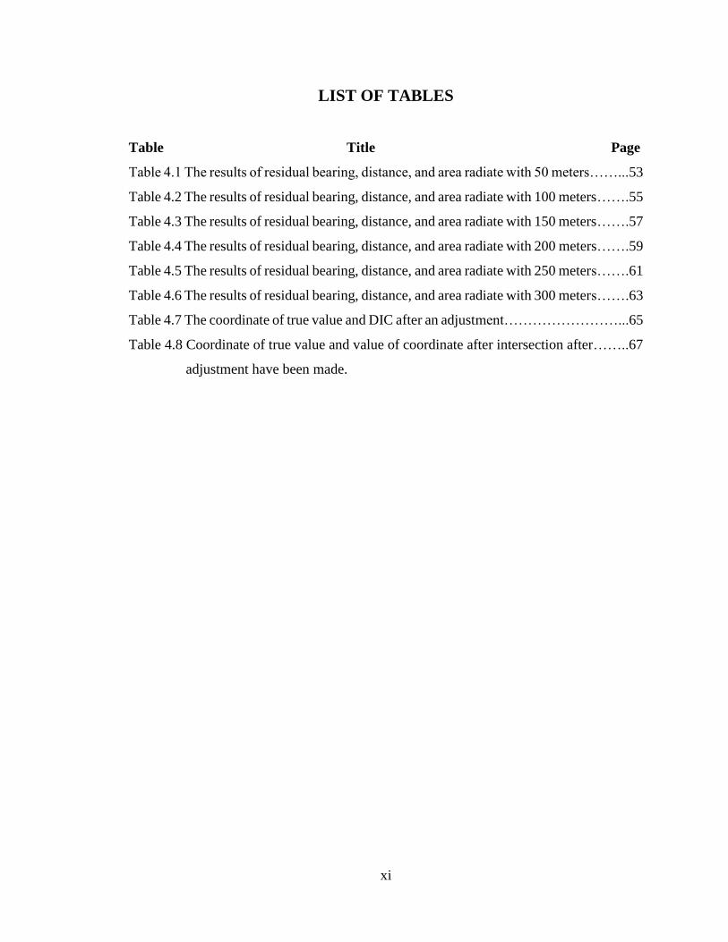
Table 4.1 The results of residual bearing, distance, and area radiate with 50 meters……...53
Table 4.2 The results of residual bearing, distance, and area radiate with 100 meters…….55
Table 4.3 The results of residual bearing, distance, and area radiate with 150 meters…….57
Table 4.4 The results of residual bearing, distance, and area radiate with 200 meters…….59
Table 4.5 The results of residual bearing, distance, and area radiate with 250 meters…….61
Table 4.6 The results of residual bearing, distance, and area radiate with 300 meters…….63
Table 4.7 The coordinate of true value and DIC after an adjustment……………………...65
Table 4.8 Coordinate of true value and value of coordinate after intersection after……..67
adjustment have been made.
xii
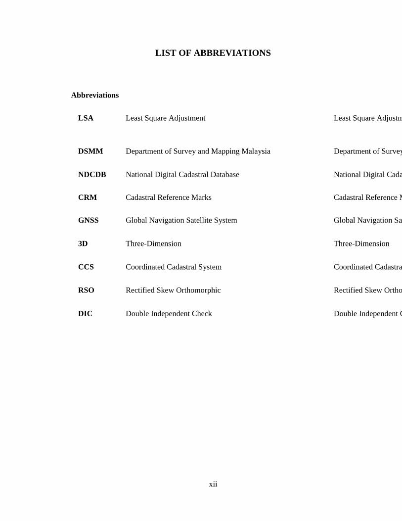
LIST OF ABBREVIATIONS
Abbreviations
LSA Least Square Adjustment Least Square Adjustment
DSMM Department of Survey and Mapping Malaysia Department of Survey and Mapping Malaysia
NDCDB National Digital Cadastral Database National Digital Cadastral Database
CRM Cadastral Reference Marks Cadastral Reference Marks
GNSS Global Navigation Satellite System Global Navigation Satellite System
3D Three-Dimension Three-Dimension
CCS Coordinated Cadastral System Coordinated Cadastral System
RSO Rectified Skew Orthomorphic Rectified Skew Orthomorphic
DIC Double Independent Check Double Independent Check

1
CHAPTER ONE
INTRODUCTION
1.1 Introduction
This chapter explained the research background, problem statement, aim and
objectives, research questions, scope and limitations of research, significance of
study and chapter outline.
1.2 Research Background
1.2.1 Radiation Method
There are several methods in plane surveying that are available in order to acquire
the data collection such as intersection method, traverse and radiation method. The
main focus in this research are radiation method. In the plane table radiation survey
method, the path of the objects or points to be located is obtained by drawing radial
lines along the fiducial edge of the alidade after the objects or points are bisected
along the alidade's line of sight. This method only suitable for the small areas and
one of method that stated by Ketua Pengarah Ukur dan Pemetaan Circular Bil
5/2009. Figure 1 shows that procedure to collect the data using the radiation
method.
Figure 1.1 Radiation method
2
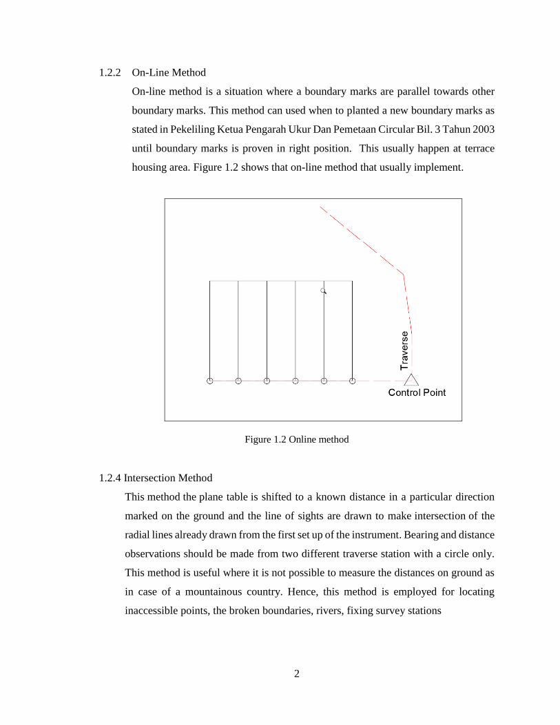
1.2.2 On-Line Method
On-line method is a situation where a boundary marks are parallel towards other
boundary marks. This method can used when to planted a new boundary marks as
stated in Pekeliling Ketua Pengarah Ukur Dan Pemetaan Circular Bil. 3 Tahun 2003
until boundary marks is proven in right position. This usually happen at terrace
housing area. Figure 1.2 shows that on-line method that usually implement.
Figure 1.2 Online method
1.2.4 Intersection Method
This method the plane table is shifted to a known distance in a particular direction
marked on the ground and the line of sights are drawn to make intersection of the
radial lines already drawn from the first set up of the instrument. Bearing and distance
observations should be made from two different traverse station with a circle only.
This method is useful where it is not possible to measure the distances on ground as
in case of a mountainous country. Hence, this method is employed for locating
inaccessible points, the broken boundaries, rivers, fixing survey stations
3
1.2.3 Bowditch Adjustment
Bowditch adjustment is a method used to adjust the control points before replacing
them with Least Square Adjustment (LSA). Bowditch is a conventional method
defined as an arbitrary method where all error estimates in linear measurements and
angular measurements are equal to the perimeter line (Yunus, Yusoff, Jamil,
Zurairah, & Halim, 2013) . The correction Bowditch method is applied based on
their uncertainties.
Least Square Adjustment is an adjustment used in traversing method where used
the mathematical model probability where basically other method did not have this
meticulous base. The sum of the squares of the errors times in minimized based on
their respective weights. Another aspect of least squares adjustment allowed all
observations even though different number or type can make an adjustment and
used simultaneously in the computation. Hence, and adjustment can be made by
can combine all the data type such as distances, horizontal angles, azimuths, zenith
or vertical angles, height differences, coordinates, and even GPS observations
(Ghilani & Wolf, 2006).
However, according to findings shows that not all of the cadastral observation
method is suitable with the LSA adjustment especially with the radiation method
in on-line since there are some are using argue that Bowditch one of adjustment
that are still widely used in cadastral surveying (Leahy, 1977).
1.3 Problem Statement
Bowditch method is method to adjust errors in bearings due to angular or linear
inaccuracies where it assumes all of observations are done to the same degree of
precision and the misclosures could be logically distributed within the survey.
While least square adjustment (LSA) is an adjustment that made solution of an
overdetermined system of equations. A least square adjustment widely used in
survey field due to its capability to determine if a survey meets acceptable
tolerances or whether the observations must be repeated (Ghilani & Wolf, 2006).
4
However, not every measurement method is suitable using LSA method since LSA
only fulfil certain condition regarding geometry checking. Bowditch adjustment
provided a geometry checking since as common to all non-least square adjustments,
any of adjustment will adjusting the angles first and the geometry will be enforced
so that their sum is correct (Sprinsky, 1987). This paper focusing on issues of
radiation method in on-line method in cadastral survey observation method.
Currently, there is no geometry data checking procedure when performing of
radiation method in on-line method Department of Survey and Mapping Malaysia
(DSMM). Thus, this research can be an enhancement for on-line method procedure
while showed the necessity of geometry data checking during cadastral survey.
1.4 Aim and Objectives
The aim of this study is on how to apply the radiation method in on-line method in
Least Square Adjustment environment.
Based on aim above, the objective as follow:
i. To study the impact of on-line method based on single leg.
ii. To study the on-line method based on geometry data checking procedure using
double independent check (DIC) and intersection method.
iii. To propose the new suggestion method procedure of geometry data checking
procedure during emplace boundary marks.
1.5 Research Question
The main objective of this study is to impact of radiation and online method in
terms of geometry checking in least square adjustment environment. In order To
achieve this main objective, some sub-objectives can be formulated:
i. What is the impact of on-line method based on single leg in LSA?
ii. What is the result of using on-line method if geometry data checking procedure
performed using double independent check (DIC) and intersection method?

5
iii. How to apply a new method of procedure for using radiation and on-line method in
least square environment?
1.6 Scope and Limitation of Research
This subsection will explain the scope of work and limitation of the research.
1.6.1 Scope of Work
This study focused on the radiation and on-line method when emplace, replace and
removed the boundary marks using these two methods. This case study is to find
out the impact differences distance of using radiation and on-line method toward
least square environment.
This study intended to cadastral practitioner, and the ins and out of this method,
when performing these two methods on land surveying.
Furthermore, it only attempted to study the impact of radiation and on-line method
and to propose the standard of procedure of geometry checking during emplace
boundary marks using radiation method and on-line method.
1.6.2 Limitations and Challenges of Research
This case study has potential limitations. First, as in most observational studies, the
work discussed here has been constrained by the methods used and time limitation.
Second, a pandemic has occured that have been prevent for data acquisition. Last
but not least, results of this study may not be completely generalizable because of
the sample size and using a simulation data which is may be vary from a real work
data.
1.7 Significance of Study
Since cadastral field required an accuracy in every observation made to be store
into National Digital Cadastral Databases (NDCDB), a geometry data checking
procedure must be conducted to make sure any of boundary marks should be within
allowable tolerance when using radiation method and on-line method. According
6
to section 369 (1) (a) in National Land Code (NLC) stated that, any boundaries
should be determined by right-lines to ensure that any of surveying works should
be conduct in manner which survey is to be carried out. By proposing a new
standard of procedure when conducting field observation radiate method for setting
out the terrace housing lot, a new geometry checking procedures should be
conducted by licensed land surveyor practitioner to ensure that the position of
boundary marks should be in right position and in allowable tolerance.
1.8 Chapter Outline
In chapter one for Introduction will present the overall planning framework such as
research background, problem statement, aim and objectives, research questions,
scope and limitations of research, significance of study for this case study.
In chapter 2 for literature review, this chapter present a review and synthesis of
methodology and findings in some of the main studies of using LSA conducted in
the past.
Next, for the chapter 3 which is Methodology highlighted planning and procedure
to approach the research questions from chapter 1. The data acquisition also
explained in this chapter.
Then, chapter 4 outline the result and analysis can be made from the data acquisition
and any findings that can be found in chapter 3. Last but not least, chapter 5 presents
a discussion of the finding in the present thesis as well as the implications in a wider
planning content, in order to provide suggestions for how to improve decision-
making.

21
CHAPTER TWO
LITERATURE REVIEW
2.1 Introduction
This chapter explain a review based on previous methodology and findings in
related studies specific to radial method in on-line, cadastral survey, observation
method, e-cadastre, issues have been highlighted in least square adjustment
environment.
2.2 Cadastral Survey
Cadastral surveying is the cadastral and a survey sub-field and is specialized in
establishing and re-establishing boundary marks in real-property boundaries for
final output which is the final title. This is an essential component of lawful
property development.
2.3 Observation Method in Bowditch Environment
2.3.1 Traverse Method
Traverse in Bowditch adjustment is a system where irregularities in
bearings may be modified due to angular or linear inaccuracies, as it
believes all measurements are always performed to the same degree of
accuracy and misclosures may be applied logically. In Bowditch
adjustment, C-correction is applying to balance the angle and traverse
adjustment. In this state, if there is no gross errors occurs in the angles and
all the systematic effect have been eliminated by instrument calibration,
careful levelling and careful instrument and target centring (Walker &
Awange, 2018).
The adjusted bearing shows that Bowditch method forced to do a correction
and the violence Bowditch does to the bearings caused serious shortcoming
of the method (Bird, 1972). As jump into conclusion least squares produces
22
more reasonable results, particularly if the final bearings are to be used to
control further work.
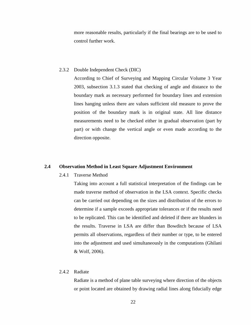
2.3.2 Double Independent Check (DIC)
According to Chief of Surveying and Mapping Circular Volume 3 Year
2003, subsection 3.1.3 stated that checking of angle and distance to the
boundary mark as necessary performed for boundary lines and extension
lines hanging unless there are values sufficient old measure to prove the
position of the boundary mark is in original state. All line distance
measurements need to be checked either in gradual observation (part by
part) or with change the vertical angle or even made according to the
direction opposite.
2.4 Observation Method in Least Square Adjustment Environment
2.4.1 Traverse Method
Taking into account a full statistical interpretation of the findings can be
made traverse method of observation in the LSA context. Specific checks
can be carried out depending on the sizes and distribution of the errors to
determine if a sample exceeds appropriate tolerances or if the results need
to be replicated. This can be identified and deleted if there are blunders in
the results. Traverse in LSA are differ than Bowditch because of LSA
permits all observations, regardless of their number or type, to be entered
into the adjustment and used simultaneously in the computations (Ghilani
& Wolf, 2006).
2.4.2 Radiate
Radiate is a method of plane table surveying where direction of the objects
or point located are obtained by drawing radial lines along fiducially edge
23
of alidade after getting the objects or points bisected along the line of sight
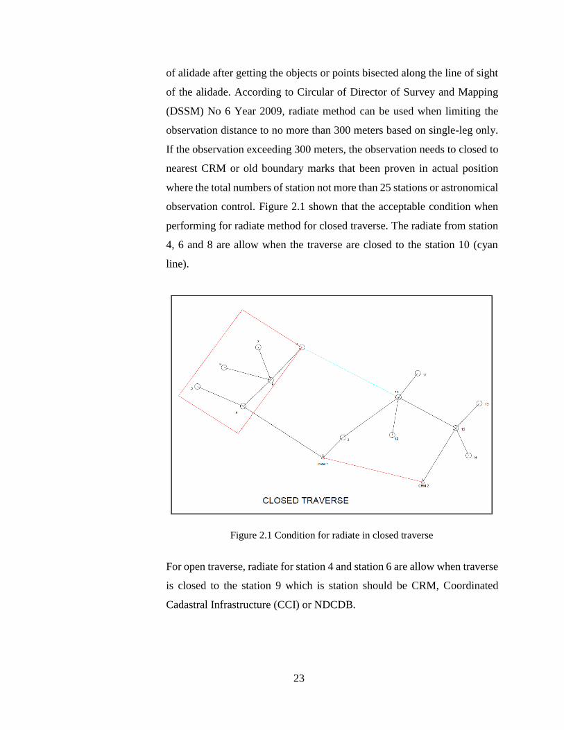
of the alidade. According to Circular of Director of Survey and Mapping
(DSSM) No 6 Year 2009, radiate method can be used when limiting the
observation distance to no more than 300 meters based on single-leg only.
If the observation exceeding 300 meters, the observation needs to closed to
nearest CRM or old boundary marks that been proven in actual position
where the total numbers of station not more than 25 stations or astronomical
observation control. Figure 2.1 shown that the acceptable condition when
performing for radiate method for closed traverse. The radiate from station
4, 6 and 8 are allow when the traverse are closed to the station 10 (cyan
line).
Figure 2.1 Condition for radiate in closed traverse
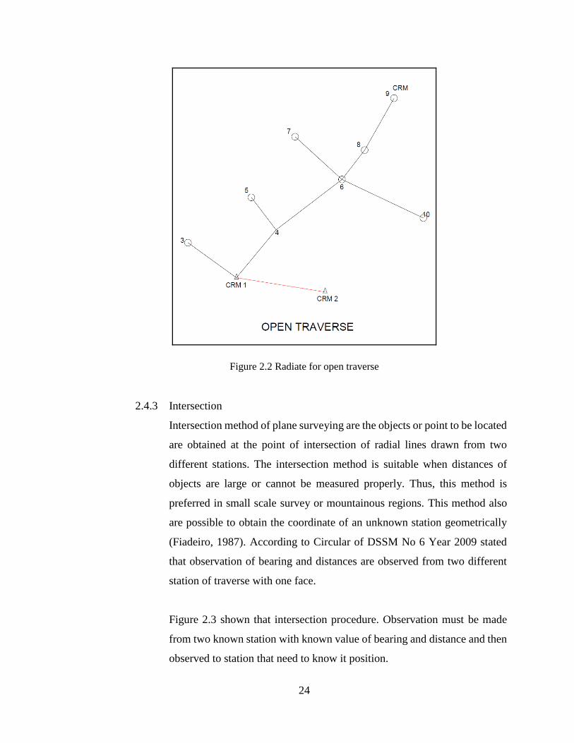
For open traverse, radiate for station 4 and station 6 are allow when traverse
is closed to the station 9 which is station should be CRM, Coordinated
Cadastral Infrastructure (CCI) or NDCDB.
24
Figure 2.2 Radiate for open traverse
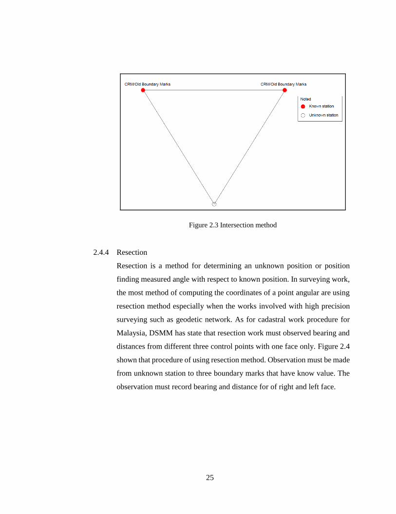
2.4.3 Intersection
Intersection method of plane surveying are the objects or point to be located
are obtained at the point of intersection of radial lines drawn from two
different stations. The intersection method is suitable when distances of
objects are large or cannot be measured properly. Thus, this method is
preferred in small scale survey or mountainous regions. This method also
are possible to obtain the coordinate of an unknown station geometrically
(Fiadeiro, 1987). According to Circular of DSSM No 6 Year 2009 stated
that observation of bearing and distances are observed from two different
station of traverse with one face.
Figure 2.3 shown that intersection procedure. Observation must be made
from two known station with known value of bearing and distance and then
observed to station that need to know it position.
25
Figure 2.3 Intersection method
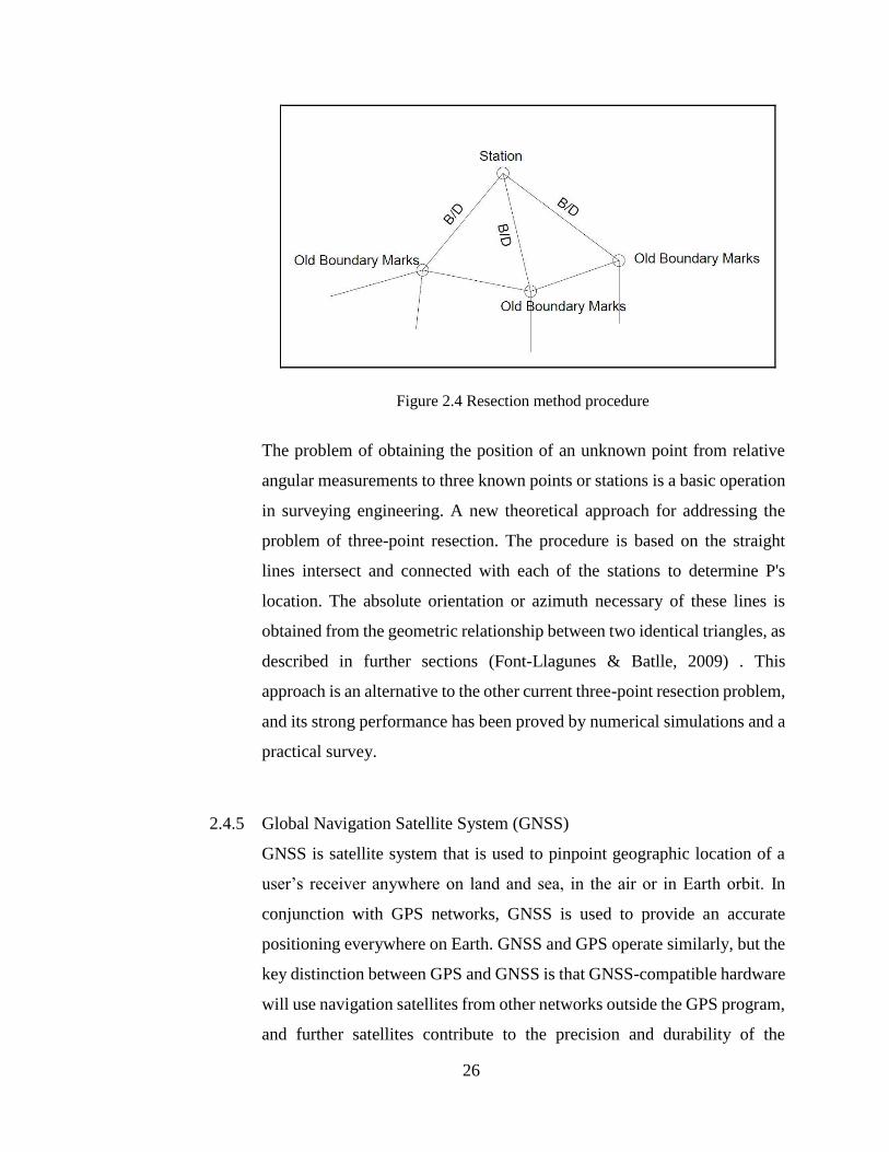
2.4.4 Resection
Resection is a method for determining an unknown position or position
finding measured angle with respect to known position. In surveying work,
the most method of computing the coordinates of a point angular are using
resection method especially when the works involved with high precision
surveying such as geodetic network. As for cadastral work procedure for
Malaysia, DSMM has state that resection work must observed bearing and
distances from different three control points with one face only. Figure 2.4
shown that procedure of using resection method. Observation must be made
from unknown station to three boundary marks that have know value. The
observation must record bearing and distance for of right and left face.
26
Figure 2.4 Resection method procedure
The problem of obtaining the position of an unknown point from relative
angular measurements to three known points or stations is a basic operation
in surveying engineering. A new theoretical approach for addressing the
problem of three-point resection. The procedure is based on the straight
lines intersect and connected with each of the stations to determine P's
location. The absolute orientation or azimuth necessary of these lines is
obtained from the geometric relationship between two identical triangles, as
described in further sections (Font-Llagunes & Batlle, 2009) . This
approach is an alternative to the other current three-point resection problem,
and its strong performance has been proved by numerical simulations and a
practical survey.
2.4.5 Global Navigation Satellite System (GNSS)
GNSS is satellite system that is used to pinpoint geographic location of a
user’s receiver anywhere on land and sea, in the air or in Earth orbit. In
conjunction with GPS networks, GNSS is used to provide an accurate
positioning everywhere on Earth. GNSS and GPS operate similarly, but the
key distinction between GPS and GNSS is that GNSS-compatible hardware
will use navigation satellites from other networks outside the GPS program,
and further satellites contribute to the precision and durability of the
27
receivers. These outdated methods of carrying out accurate horizontal
control surveys have been gradually replaced by the GPS. In addition, not
only does GPS produce horizontal positions but it also produces ellipsoidal
heights. So, three-dimensional surveys are given by GPS. Like in all
remarks, the GPS results contain mistakes and need to be modified (Ghilani
& Wolf, 2006).
The application of LSA in GPS can be seen when used to as online quality
control of Multi-GNSS real-time clock estimation. Real-time satellite orbit
and clock product is a key prerequisite for real-time precise positioning
service based on precise point positioning (PPP). With the growth
development of the multiple global navigation satellite systems (Multi-
GNSS), there are almost 120 satellites will be processed for Multi-GNSS
real-time clock estimation (Fu et al., 2019). Unfortunately, the computation
is very time-consuming, especially for quality control since problematic
observations are inevitable. Sequential square sequential adjustment with
an adapted online quality control system is developed to quickly estimate
Multi-GNSS real-time clocks, although specific filtering estimators are now
commonly used.
Cycle slip detection for single frequency GNSS data is currently focused
largely on measurement modeling or estimation that cannot be effectively
done for kinematic applications and minor cycle slips such as half-cycle
slips are difficult to detect or repair (Chen, Chen, Jiang, Zhou, & Yuan,
2018). A new technique based on the total differential of ambiguity and
Least-Squares Adjustment (LSA) for cycle slip detection and repair is
introduced and validated. LSA is then performed to diagnose and fix cycle
slips where the coordinate and cycle slips are obtained.
28
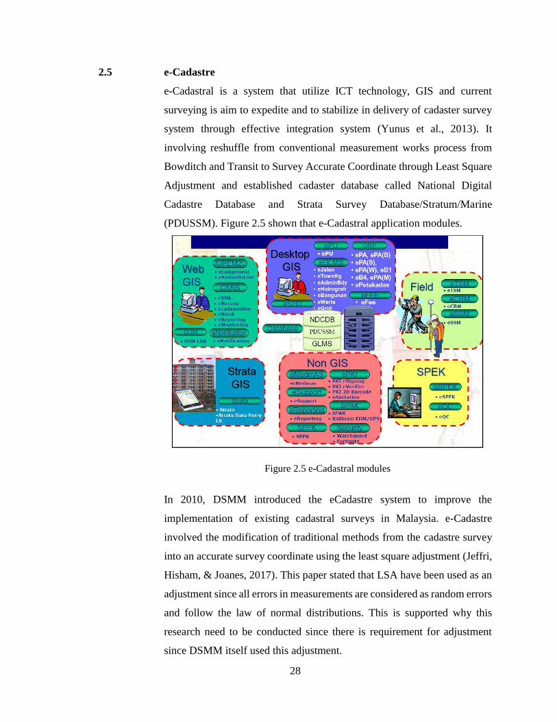
2.5 e-Cadastre
e-Cadastral is a system that utilize ICT technology, GIS and current
surveying is aim to expedite and to stabilize in delivery of cadaster survey
system through effective integration system (Yunus et al., 2013). It
involving reshuffle from conventional measurement works process from
Bowditch and Transit to Survey Accurate Coordinate through Least Square
Adjustment and established cadaster database called National Digital
Cadastre Database and Strata Survey Database/Stratum/Marine
(PDUSSM). Figure 2.5 shown that e-Cadastral application modules.
Figure 2.5 e-Cadastral modules
In 2010, DSMM introduced the eCadastre system to improve the
implementation of existing cadastral surveys in Malaysia. e-Cadastre
involved the modification of traditional methods from the cadastre survey
into an accurate survey coordinate using the least square adjustment (Jeffri,
Hisham, & Joanes, 2017). This paper stated that LSA have been used as an
adjustment since all errors in measurements are considered as random errors
and follow the law of normal distributions. This is supported why this
research need to be conducted since there is requirement for adjustment
since DSMM itself used this adjustment.

29
A case study has been conducted at Malaysia relating standard provides of
conceptual model for recording and managing land administration data
which called land administration domain model (LADM). This offers an
extensible framework for the implementation and improvement of land
management systems functionality and effectiveness, based on a Model
Driven Architecture (MDA) which helps the participants to interact which
infer the model, both within one country and between various countries.
(Rajabifard et al., 2018). The inducement for this paper is to address
Malaysian government's new initiative to explore the realistic road to
realizing a LADM-based 3D cadastral system in accordance with
Malaysia's jurisdictional settings. The paper also proposed how 3D-
NDCDB's action plan, including enhancing current database and methods
of data collection to promote digital data based on user requirement. These
approaches will enhance the integration of complementing modules such as
3D spatial data input, 3D adjustment and validation of 3D spatial data.
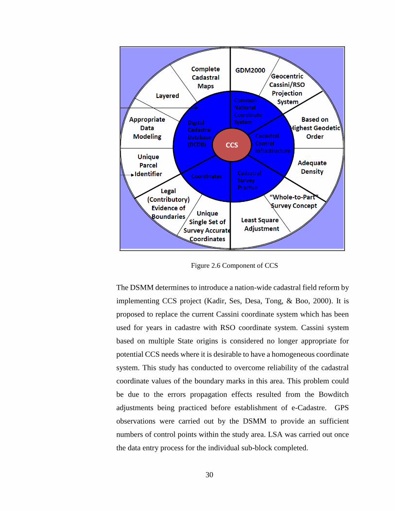
2.5.1 Coordinated Cadastral System (CCS)
There are three main components in e-Cadastre to be specific Coordinated
Cadastral System (CCS), Virtual Survey System and Cadastral Data
Integrity System. The implementation of CCS is a major part of the e-
Cadastre project that includes field and office reengineering to reduce
processes and increase the use of digital technology. Figure 2.6 shown that
characteristic (blue) of CCS and their aspects (white).
30
Figure 2.6 Component of CCS
The DSMM determines to introduce a nation-wide cadastral field reform by
implementing CCS project (Kadir, Ses, Desa, Tong, & Boo, 2000). It is
proposed to replace the current Cassini coordinate system which has been
used for years in cadastre with RSO coordinate system. Cassini system
based on multiple State origins is considered no longer appropriate for
potential CCS needs where it is desirable to have a homogeneous coordinate
system. This study has conducted to overcome reliability of the cadastral
coordinate values of the boundary marks in this area. This problem could
be due to the errors propagation effects resulted from the Bowditch
adjustments being practiced before establishment of e-Cadastre. GPS
observations were carried out by the DSMM to provide an sufficient
numbers of control points within the study area. LSA was carried out once
the data entry process for the individual sub-block completed.
31
The CCS have been discussed on (Teoh, 2009) paper about construction
and development of a Malaysian Geographic Information System (GIS)
database repository for location data sources accessible in Malaysia. This
paper addressed problems with the use of different data in surveys and
cadasters, not only caused inconveniences such as the migration from RSO
to Cassini, but also created questions about data incompatibility with
existing satellite navigation systems. Writer proposed Location based
System (LBS) that allows a user to search, identify and check for location
information. In order to improve the conversion of coordinate
transformation has address by writer, it is better to precompute and build
lookup tables for faster results.
2.5.2 National Digital Cadastre Database (NDCDB)
The National Digital Cadastral Survey Database (NDCDB) is a new digital
platform for land surveying database replacing the Digital Cadastral Survey
Database (DCDB). The information shown in the database such as Unique
Parcel Identifier (UPI), lot number, area and lot boundary information. The
format is in vector graphics format for example *.shp, *.tab, *.dxf, *.dgn
and others.
Several studies have been conducted to study the NDCDB. One study that
have been conducted is the handling of NDCDB with GIS application by
(Abdul Halim, Sulaiman, Talib, & Majeed, 2018). The technique used was
a case study duplicated to five establishment of GIS applications from
different agencies such as eKadasOnline, SKiP, iPlan, TM SmartMap and
DBKL Interactive Portal. Some suggestions that highlighted in this paper to
rectify knowledge-based mistakes found in this study, that included the
ensuring the NDCDB’s cut-off-date, utilizes all existing NDCDB layers,
ensure to use the map projection parameters are the authorized and official
value. Based on the data from the multi-case report, the rival propositions
were considered to be more appropriate for summarizing the overall results,
32
which were certain methods of applying NDCDB for land-based spatial
analysis as certain users had a partial understanding of the NDCDB
properties.
Another study that have been conducted to NDCDB on GIS application is
identifying the relevant features of the (NDCDB) for spatial analysis by
using the Delphi Technique by (N. Z.A. Halim, Sulaiman, Talib, & Ng,
2018). In this paper the Delphi methodology approach is considerably
explored. This research has achieved its objective of defining statements
that better explain the related features of NDCDB for spatial analysis by
optimizing the Delphi methodology based on the consensus of experts on
ground, cadastral and GIS domain. Agreement and stability of the
consensus on the statements were achieved.
This Delphi techniques method also apply on (Nur Zurairah Abdul Halim
et al., 2017) paper about the Legal significance of National Digital Cadastral
Database (NDCDB) in Malaysia Cadastral System. To determine the legal
significance of NDCDB and evaluate its key themes, insights, and
judgements on a collective basis from diverse expertise seemed suitable.
This work has provided clarity about the implementation of NDCDB, at
least where the issue is legal comparison. From the analysis it can be
summarized that NDCDB does not have a clear legal relation for boundary
description but as an option for boundary comparisons to a particular spatial
tolerance and is also one of the many approved cadastral databases used in
DSMM.
2.6 Online Observation
On-line method is a situation where a boundary marks are parallel towards other
boundary marks. This method can used when to planted a new boundary marks as
stated in Pekeliling Ketua Pengarah Ukur Dan Pemetaan Circular Bil. 3 Tahun 2003
33
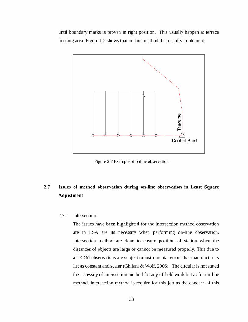
until boundary marks is proven in right position. This usually happen at terrace
housing area. Figure 1.2 shows that on-line method that usually implement.
Figure 2.7 Example of online observation
2.7 Issues of method observation during on-line observation in Least Square
Adjustment
2.7.1 Intersection
The issues have been highlighted for the intersection method observation
are in LSA are its necessity when performing on-line observation.
Intersection method are done to ensure position of station when the
distances of objects are large or cannot be measured properly. This due to
all EDM observations are subject to instrumental errors that manufacturers
list as constant and scalar (Ghilani & Wolf, 2006). The circular is not stated
the necessity of intersection method for any of field work but as for on-line
method, intersection method is require for this job as the concern of this

34
study to prove the requirement for this method when performing on-line
method.
2.7.2 Resection
The issues of resection exactly have the same issues as subsection 2.7.1.
Both of resection and intersection are necessary when performing on-line
method during surveying works to ensure the placement of boundary marks
are placed in right position as to ensure the accuracy of survey works. These
two methods are proposed when performing on-line is due to ensure the
reliability value of coordinates of boundary marks.
2.7.3 Radiate
Radiate is common method using when performing on-line method. The
radiate method usually performed especially when to place the boundary
marks. The issues of radiate itself doubting its reliability of this method
during survey works. This is due to the radiate does not have geometrically
checking as resection and intersection method. After an adjustment have
been made using least square, the value of bearing and distance have been
differed from the original one. The maximum distance when performing
radiate are 300 meters. What are the effects towards value of bearing,
distance and coordinate when performing radiate in on-line method based
on short and long distance? These are the main issues of radiate in on-line
method if least square are be used for the adjustment.
2.8 Conclusion
The important aspects of the existing this literature review is to identify the work
contribution for better understanding the research problem being studied. Based on
research in this literature review, any of method have been describe the relationship
of each method studied to the others consideration. This is important to locate this

35
research within the context of existing literature and to prevent the duplication of
effort.
The method used in this study have been reviewed and the gaps in existing studied
have been identified for better improvement in this research. For future study, the
suggested method should be implement in this research which is radiate method in
on-line method in Least Square Adjustment.
The findings of this literature review have shown that the gaps in on-line method
procedure where there is no geometry data checking when performing radiate
method. Others study found that there are disadvantages of least square adjustment
in other method such as GNSS and may affect the NDCDB which the main hub of
geospatial data.
36
CHAPTER THREE
METHODOLOGY
3.1 Introduction
This chapter will emphasis the methodology and flowchart in order to achieve the
aim and objectives of this research works, there are several of data processing had
been done. The methodology of this project is divided into five (5) main phases
such as i) planning, ii) data acquisition, iii) data processing, iv) result and analysis
and v) conclusion.
3.2 Preliminary Studies
The first thing that needs to be done during Step 1 is to develop the concept for the
project title. Until identifying the required criteria, it is necessary to identify aim
and objectives while simplifying the name. In the literature review, these
parameters needed to be brief in detail so that the information and idea can be added
smartly and the understanding of the project can be firmly established. This study
is focusing on the impact on radiation and on-line method in cadastral observation
method and its suitability in least square adjustment. The procedure, software and
parameter required to execute this research were also determined. This phase ended
with the execution of data processing by using Micro STARNet software to achieve
the aim and objectives of study.
3.2.1 Data acquisition
The data for this research used a secondary data which is simulation data. The data
was designated using CAD software which is AutoCAD version 2016. The traverse
data was designated on CAD software replacing the real job since there are
limitation for acquiring data on site. A closed traverse was drawn on AutoCAD
while following the standard tolerance according to JUPEM’s circular. The data
that have been used for this research is bearing, distance, area and coordinate.

37
3.2.2 Software used
The software used to complete this study are AutoCAD version 2016, MicroSurvey
STARNet software, Microsoft Excel and IBM SPSS Statistic software.
i. CAD software
AutoCAD is a software framework for engineering computer-aided design
(CAD) and drafting. AutoCAD 2016 was used for designing the simulation
data which are traverse and method of acquire the housing’s boundary
marks which radiate and intersection method. Figure 3.1 shows that
AutoCAD 2016 used in this research.
Figure 3.1 CAD software used for this research
ii. Microsoft Excel
Microsoft Excel used in this research when all form data need to be extract
from the AutoCAD software. The data extraction function from AutoCAD
can be extract into of (.xlsv) format. The Microsoft Excel itself was used to
calculate the value of bearing from degree minute second format
(00°00′00") to radian. Micosoft Excel also used to classify all of the
bearing, distance, area and coordinate of each boundary marks.

38
iii. MicroSurvey’s STAR*NET
MicroSurvey's STAR*NET is the least square adjustment software
recognized in the world. STAR*NET has earned a reputation as a
manufacturer of least square correction solutions for being easy to use,
highly accurate and reliable. The results of STAR*NET serve as the
industry benchmark and are prescribed as the mandatory package of
adjustments in some jurisdictions when used in the submission of plans.
Figure 3.2 shows that software was used in this study.
Figure 3.2 Software used
iv. IBM SPSS Statistic
SPSS Statistics is a leading statistical app, is equipped for ad hoc modeling,
hypothesis testing, geospatial modeling and predictive analytics to solve
market and science problems. IBM SPSS Statistic was used to calculate
statistical value mean, minimum, maximum, range, and standard deviation
of residual bearing, residual distance, residual area and residual coordinate.
39
Figure 3.3 IBM SPSS Statistic
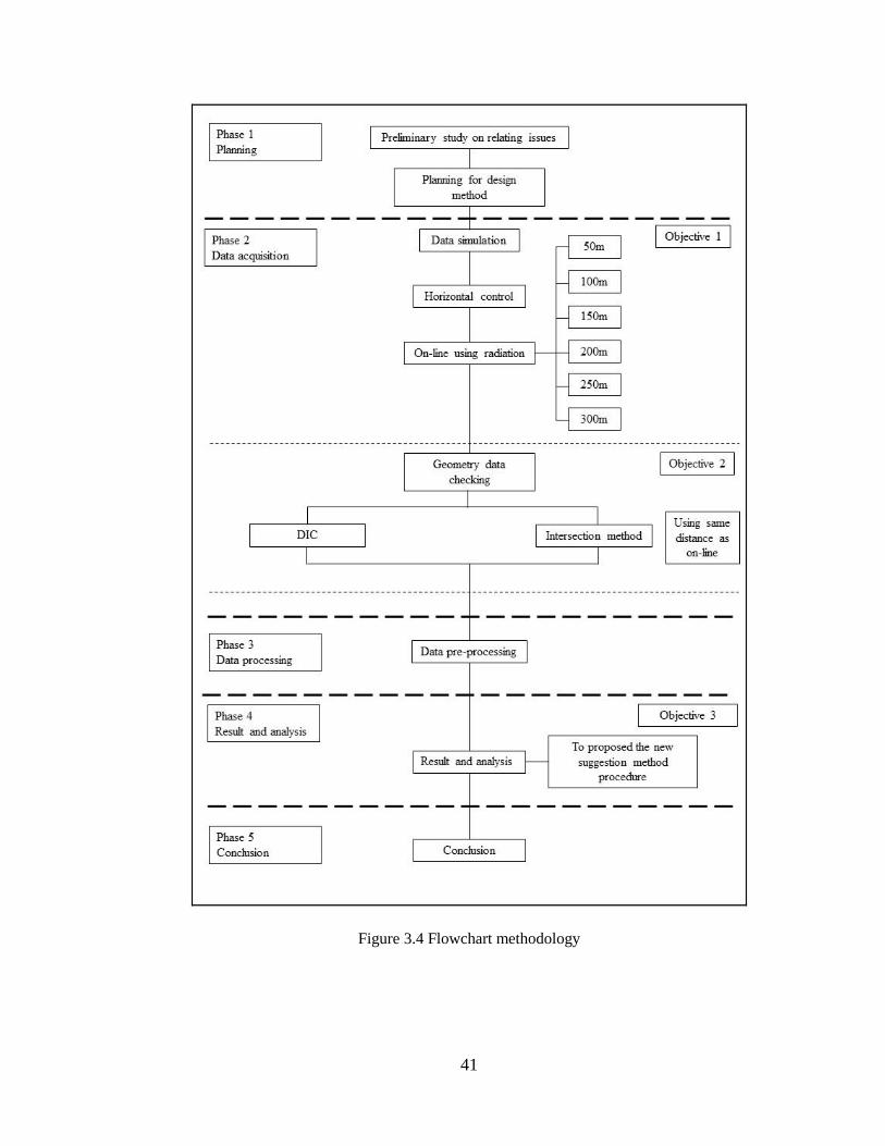
3.3 Flowchart of methodology
In order to achieve the aim and objectives of this research works, there are several
of data processing had been done. Figure illustrates the general methodology of this
research. The methodology of this project is divided into five (5) main phases such
as i) planning, ii) data acquisition, iii) data processing, iv) result and analysis and
v) conclusion.
The methodology of this study consists of five phases as shown in Figure 1. The
four five phases are planning, data acquisition, data processing, result and analysis,
and conclusion. The first phase is focusing on the issues and problem of the study.
In this phase, the method, type of data and in order to perform data acquisition is
identified and listed out.
The second phase is known as data simulation. In order to achieve the objectives of
this study, horizontal control established and to achieve the first objectives which
is using radiation based on single leg method. A several different distances have
been using to find out the impact on radiation method based on single leg. The
40
second objective is to study the impact of geometry data checking using double
independent check (DIC) and intersection method. The same distance as in first
method were used to test this geometry data checking method which are 50m,
100m, 150m, 200m, 250m and 300m.
These data will undergo data processing phase using LSA software. Next, result
and analysis process. In this process, the data is process based on aim and the
objectives of the study. By the end of this phase, a new suggestion will be made
which are to propose the new method of procedure of on-line and radiation method.
Last but not least, the conclusion phase. From the analysis made, this can study can
be concluded to be achieve its aim or not. Figure 3.4 shows that flowchart of
research methodology involves in this study.
41
Figure 3.4 Flowchart methodology

42
3.4 Design of simulation data
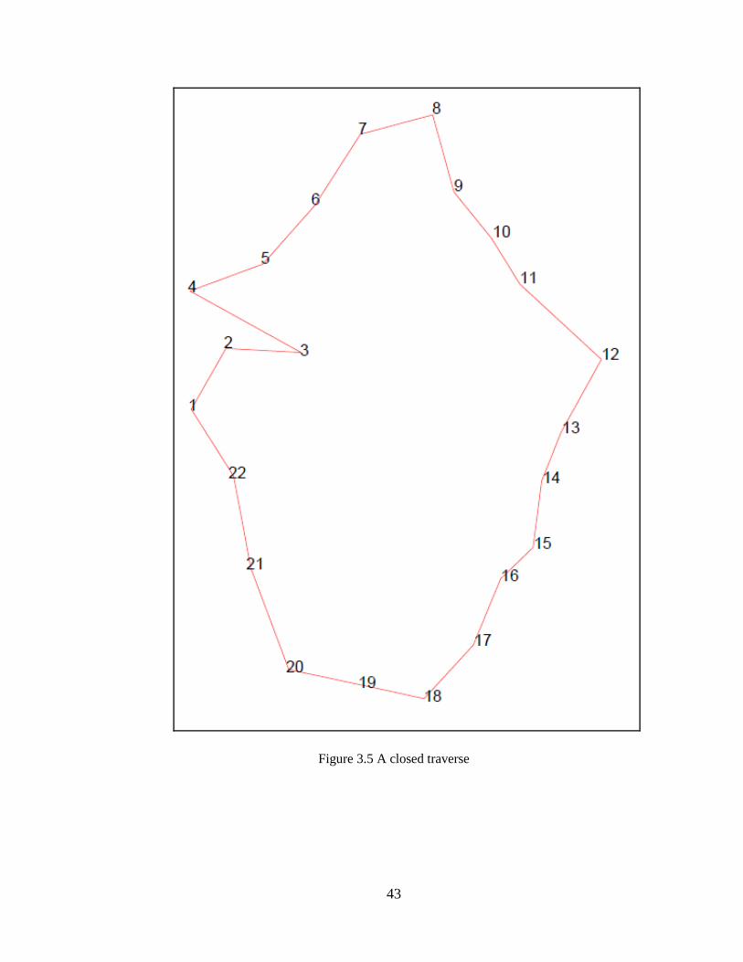
A closed traverse was designated using CAD software following the JUPEM’s circular
based on its tolerance. Both of face right and face left should be not more than
00°00′20" and distance not more than 0.01m. There are about 22 horizontal control
points established using AutoCAD software. Figure 3.5 shows that a closed traverse
design on AutoCAD 2016 software.
Then, seven housing lot with standard dimension 23 𝑓𝑡 × 70 𝑓𝑡 or 7.315𝑚 ×
21.336𝑚 was designated in the middle of the traverse so that the next step for research
can be conducted. The next procedure was performed a radiate method from control
points to housing lot boundary marks with distance 50m, 100m, 150m, 200m, 250m
and 300m. Appendix A until Appendix F is the input file (.txt) for every distance
mentioned.
Station 3 was radiate with average 50m, station 5 radiated with 100m, station 9
radiated with 150m, station 13 radiated with 200m, station 16 radiated with distance
250m and lastly station 20 was radiated with the maximum distance 300m. All of input
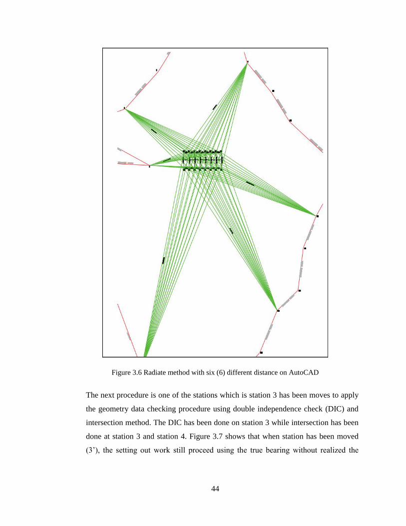
file for these distances are given on Appendix. Figure 3.6 shows illustrator of what
surveyor normally do when emplacing the boundary marks for terrace housing lot.
Figure 3.6 shows that radiation method was used to for simulation data. Appendix G
is input file DIC geometry data checking and Appendix I is for intersection method
input file (.txt).
43
Figure 3.5 A closed traverse
44
Figure 3.6 Radiate method with six (6) different distance on AutoCAD
The next procedure is one of the stations which is station 3 has been moves to apply
the geometry data checking procedure using double independence check (DIC) and
intersection method. The DIC has been done on station 3 while intersection has been
done at station 3 and station 4. Figure 3.7 shows that when station has been moved
(3’), the setting out work still proceed using the true bearing without realized the

45
station 3 has been moved. In order to check whether the station have been moved or
not, the surveyor apply the DIC and intersection method.
Figure 3.7 Lot has been moved from the actual position

46
3.5 Data Processing
Data processing is a method of evaluating information either analytical and
statistical tools to search for helpful data for produce a method of procedure as an
conclusion. This tools enables to explore for information, notice patterns in it and
answer any question on it. For this study, a simulation data was used and all of data
was processed using accurate statistical method.
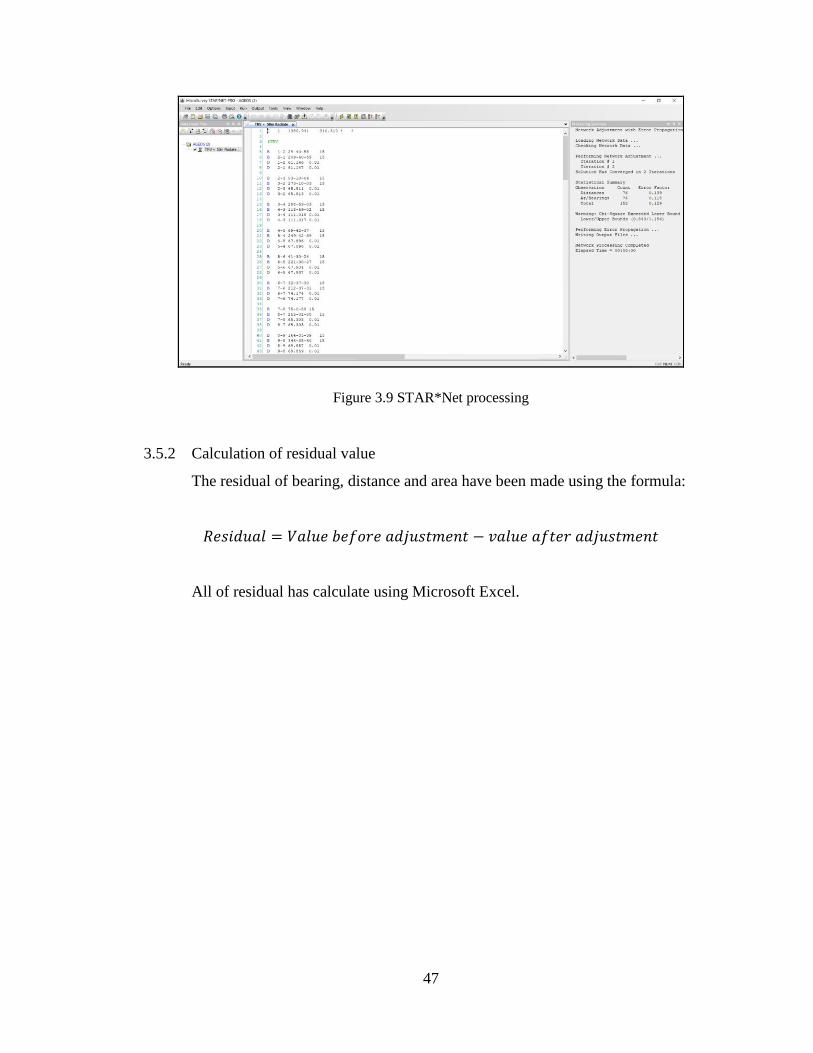
3.5.1 Least Square Adjustment
As for JUPEM have go from Bowditch to LSA, an adjustment has been made using
STAR*Net software. Six input files have been created as using (.txt) where all the
data such as bearing, distance and coordinate from traverse and radiate have been
inserted. Figure 3.7 shows that example of input file using (.txt) of traverse and
radiate with distance 50m. The rest of input file as stated in Appendix section. Then,
the input file has been imported to STAR*Net software to run adjustment. Figure
3.8 shows that processing of
Figure 3.8 Examples of input file of traverse and radiate with distance 50m
47
Figure 3.9 STAR*Net processing
3.5.2 Calculation of residual value
The residual of bearing, distance and area have been made using the formula:
𝑅𝑒𝑠𝑖𝑑𝑢𝑎𝑙 = 𝑉𝑎𝑙𝑢𝑒 𝑏𝑒𝑓𝑜𝑟𝑒 𝑎𝑑𝑗𝑢𝑠𝑡𝑚𝑒𝑛𝑡 − 𝑣𝑎𝑙𝑢𝑒 𝑎𝑓𝑡𝑒𝑟 𝑎𝑑𝑗𝑢𝑠𝑡𝑚𝑒𝑛𝑡
All of residual has calculate using Microsoft Excel.
48
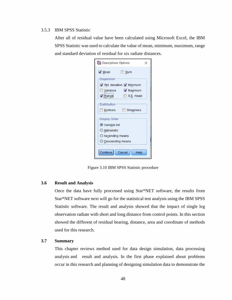
3.5.3 IBM SPSS Statistic
After all of residual value have been calculated using Microsoft Excel, the IBM
SPSS Statistic was used to calculate the value of mean, minimum, maximum, range
and standard deviation of residual for six radiate distances.
Figure 3.10 IBM SPSS Statistic procedure
3.6 Result and Analysis
Once the data have fully processed using Star*NET software, the results from
Star*NET software next will go for the statistical test analysis using the IBM SPSS
Statistic software. The result and analysis showed that the impact of single leg
observation radiate with short and long distance from control points. In this section
showed the different of residual bearing, distance, area and coordinate of methods
used for this research.
3.7 Summary
This chapter reviews method used for data design simulation, data processing
analysis and result and analysis. In the first phase explained about problems
occur in this research and planning of designing simulation data to demonstrate the

49
problem as stated in problem statement. Then, the second phase discusses about the
method used in data simulation. Third phase explained about data processing using
Star*NET and IBM SPSS Statistic software. This software used to enhance the
realiability . Last result from the study.
50
CHAPTER FOUR
RESULT AND ANALYSIS
4.1 Introduction
4.2 Result
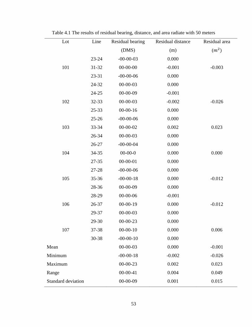
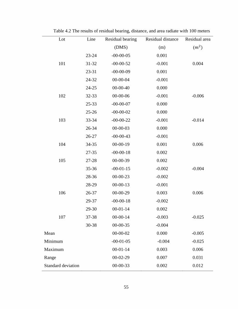
4.2.1 Residual bearing, distance and area of radiate method
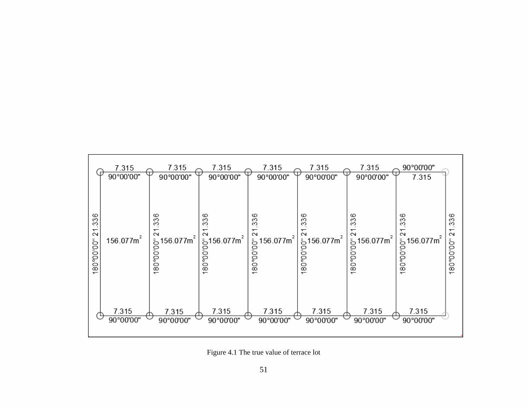
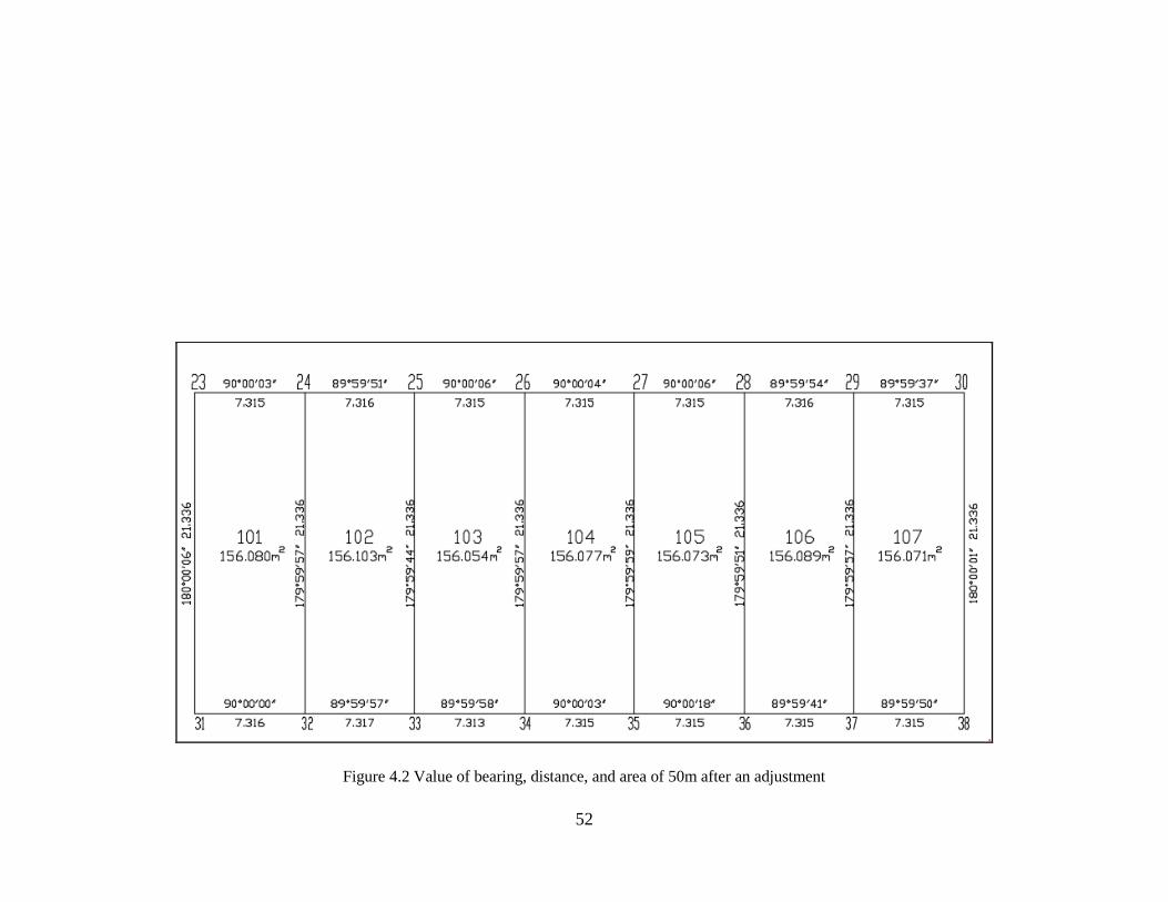
Table 4.1 until Table 4.6 shows that result of residual after been computed using
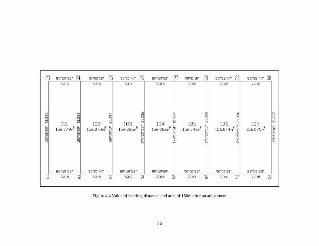
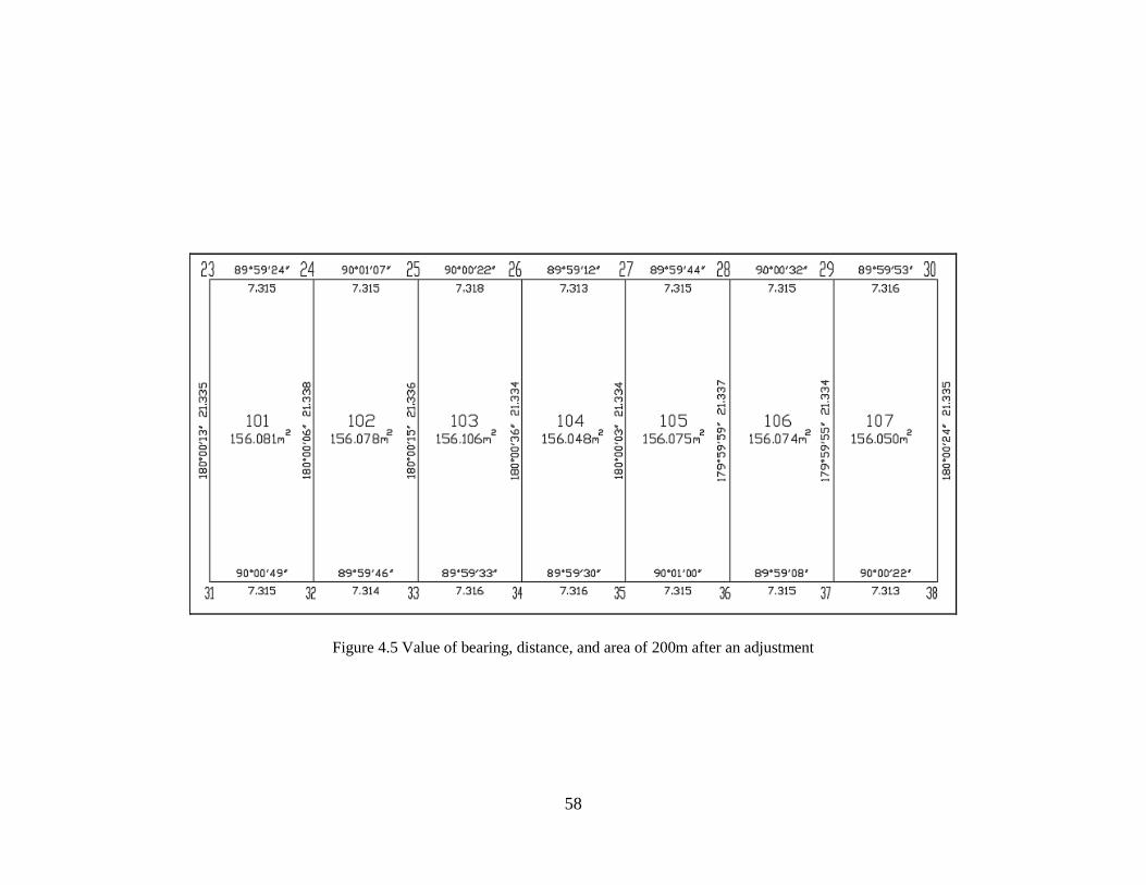
IBM SPSS Statistic software. Figure 4.1 shows that true value of lot before
adjustment and Figure 4.2 until Figure 4.7 shows that value of lot with bearing,
distance and area that have been radiate with distance 50m, 100m, 150m, 200m,
250m and 300m.
51
Figure 4.1 The true value of terrace lot
52
Figure 4.2 Value of bearing, distance, and area of 50m after an adjustment
53
Table 4.1 The results of residual bearing, distance, and area radiate with 50 meters
Lot Line Residual bearing
(DMS)
Residual distance
(m)
Residual area
(𝑚2)
101
23-24 -00-00-03 0.000
-0.003
31-32 00-00-00 -0.001
23-31 -00-00-06 0.000
24-32 00-00-03 0.000
102
24-25 00-00-09 -0.001
-0.026 32-33 00-00-03 -0.002
25-33 00-00-16 0.000
103
25-26 -00-00-06 0.000
0.023 33-34 00-00-02 0.002
26-34 00-00-03 0.000
104
26-27 -00-00-04 0.000
0.000 34-35 00-00-0 0.000
27-35 00-00-01 0.000
105
27-28 -00-00-06 0.000
-0.012 35-36 -00-00-18 0.000
28-36 00-00-09 0.000
106
28-29 00-00-06 -0.001
-0.012 26-37 00-00-19 0.000
29-37 00-00-03 0.000
107
29-30 00-00-23 0.000
0.006 37-38 00-00-10 0.000
30-38 -00-00-10 0.000
Mean 00-00-03 0.000 -0.001
Minimum -00-00-18 -0.002 -0.026
Maximum 00-00-23 0.002 0.023
Range 00-00-41 0.004 0.049
Standard deviation 00-00-09 0.001 0.015

54
Figure 4.3 Value of bearing, distance, and area of 100m after an adjustment
55
Table 4.2 The results of residual bearing, distance, and area radiate with 100 meters
Lot Line Residual bearing
(DMS)
Residual distance
(m)
Residual area
(𝑚2)
101
23-24 -00-00-05 0.001
0.004 31-32 -00-00-52 -0.001
23-31 -00-00-09 0.001
24-32 00-00-04 -0.001
102
24-25 00-00-40 0.000
-0.006 32-33 00-00-06 -0.001
25-33 -00-00-07 0.000
103
25-26 -00-00-02 0.000
-0.014 33-34 -00-00-22 -0.001
26-34 00-00-03 0.000
104
26-27 -00-00-43 -0.001
0.006 34-35 00-00-19 0.001
27-35 -00-00-18 0.002
105 27-28 00-00-39 0.002
-0.004 35-36 -00-01-15 -0.002
28-36 00-00-23 -0.002
106
28-29 00-00-13 -0.001
0.006 26-37 00-00-29 0.003
29-37 -00-00-18 -0.002
107
29-30 00-01-14 0.002
-0.025 37-38 00-00-14 -0.003
30-38 00-00-35 -0.004
Mean 00-00-02 0.000 -0.005
Minimum -00-01-05 -0.004 -0.025
Maximum 00-01-14 0.003 0.006
Range 00-02-29 0.007 0.031
Standard deviation 00-00-33 0.002 0.012
56
Figure 4.4 Value of bearing, distance, and area of 150m after an adjustment

57
Table 4.3 The results of residual bearing, distance, and area radiate with 150 meters
Lot Line Residual bearing
(DMS)
Residual distance
(m)
Residual area
(𝑚2)
101
23-24 00-00-28 -0.001
-0.002 31-32 00-00-02 0.000
23-31 -00-00-02 0.001
24-32 -00-00-09 0.000
102 24-25 -00-01-20 0.000
0.004 32-33 -00-00-47 0.001
25-33 -00-00-13 -0.001
103 25-26 -00-00-47 0.000
-0.008 33-34 00-00-04 -0.001
26-34 00-00-07 0.000
104 26-27 00-00-10 0.00
0.011 34-35 00-00-51 0.000
27-35 00-00-09 0.002
105 27-28 -00-01-10 0.000
0.031 35-36 -00-00-33 0.001
28-36 00-00-02 0.003
106 28-29 00-01-13 0.000
0.003 26-37 -00-00-03 -0.001
29-37 00-00-08 0.000
107 29-30 00-01-13 0.000
0.002 37-38 00-00-27 0.000
30-38 00-00-12 -0.001
Mean 00-00-03 0.000 0.006
Minimum -00-01-10 -0.001 -0.008
Maximum 00-01-13 0.003 0.031
Range 00-02-23 0.004 0.039
Standard deviation 00-00-35 0.001 0.013
58
Figure 4.5 Value of bearing, distance, and area of 200m after an adjustment

59
Table 4.4 The results of residual bearing, distance, and area radiate with 200 meters
Lot Line Residual bearing
(DMS)
Residual distance
(m)
Residual area
(𝑚2)
101
23-24 00-00-36 0.000
-0.004 31-32 -00-00-49 0.000
23-31 -00-00-13 0.001
24-32 -00-00-06 -0.002
102 24-25 -00-01-07 0.000
-0.001 32-33 00-00-14 0.001
25-33 -00-00-15 0.000
103 25-26 -00-00-22 -0.003
-0.029 33-34 00-00-27 -0.001
26-34 -00-00-36 0.002
104 26-27 00-00-48 0.002
0.029 34-35 00-00-30 -0.001
27-35 -00-00-30 0.002
105 27-28 00-00-16 0.000
0.002 35-36 00-00-06 0.000
28-36 00-00-01 -0.001
106 28-29 -00-00-32 0.000
0.003 26-37 00-00-52 0.000
29-37 00-00-05 0.002
107 29-30 00-00-07 -0.001
0.027 37-38 -00-00-22 0.002
30-38 -00-00-24 0.001
Mean 00-00-50 0.000 0.004
Minimum -00-01-07 -0.003 -0.029
Maximum 00-00-52 0.002 0.029
Range 00-01-59 0.005 0.058
Standard deviation 00-00-33 0.001 0.020

60
Figure 4.6 Value of bearing, distance, and area of 250m after an adjustment

61
Table 4.5 The results of residual bearing, distance, and area radiate with 250 meters
Lot Line Residual bearing
(DMS)
Residual distance
(m)
Residual area
(𝑚2)
101
23-24 00-00-12 -0.001
-0.043 31-32 -00-01-56 -0.003
23-31 -00-00-22 0.002
24-32 -00-00-04 -0.003
102
24-25 -00-00-34 0.000
0.012 32-33 00-00-39 0.002
25-33 -00-00-18 0.000
103
25-26 -00-00-21 -0.001
-0.012 33-34 00-00-12 -0.001
26-34 -00-00-1 0.001
104
26-27 -00-00-19 0.002
0.014 34-35 -00-00-45 -0.001
27-35 00-00-12 0.000
105
27-28 00-00-12 -0.002
-0.002 35-36 00-00-40 0.001
28-36 -00-00-14 0.001
106
28-29 -00-01-18 0.000
0.012 26-37 -00-00-07 -0.001
29-37 -00-00-04 0.004
107
29-30 00-02-41 -0.002
-0.004 37-38 00-00-05 0.000
30-38 -00-00-24 0.000
Mean -00-00-06 0.000 -0.003
Minimum -00-01-56 -0.003 -0.043
Maximum 00-02-41 0.004 0.014
Range 00-04-37 0.007 0.057
Standard deviation 00-00-51 0.002 0.020

62
Figure 4.7 Value of bearing, distance, and area of 250m after an adjustment

63
Table 4.6 The results of residual bearing, distance, and area radiate with 300 meters
Lot Line Residual bearing
(DMS)
Residual distance
(m)
Residual area
(𝑚2)
101
23-24 -00-00-17 -0.001
-0.002 31-32 -00-00-29 0.000
23-31 00-00-44 0.001
24-32 00-00-27 0.000
102
24-25 -00-00-05 -0.005
-0.064 32-33 -00-00-13 -0.002
25-33 00-00-00 0.000
103
25-26 00-00-11 -0.002
-0.001 33-34 00-00-12 0.002
26-34 -00-00-34 0.000
104
26-27 00-00-10 0.000
-0.009 34-35 00-00-11 -0.001
27-35 -00-00-25 0.000
105
27-28 -00-00-30 0.008
0.056 35-36 -00-01-32 -0.002
28-36 00-01-14 -0.002
106
28-29 00-00-08 -0.009
-0.093 26-37 00-01-11 0.001
29-37 -00-00-22 0.000
107
29-30 -00-01-29 -0.004
-0.075 37-38 -00-01-14 -0.003
30-38 -00-00-32 0.000
Mean -00-00-09 -0.01 -0.027
Minimum -00-01-32 -0.009 -0.093
Maximum 00-01-14 0.008 0.056
Range 00-02-46 0.017 0.149
Standard deviation 00-00-43 0.003 0.053

64
4.2.2 Double Independence Check (DIC)
Figure 4.1 shows that Chi Square Test of double independence check at station 3
without move the station 3 while Figure 4.2 shows that Chi Square Test of double
independence check at station 3 when station 3 has been moved.
Figure 4.8 Chi Square Test of true value when checking with DIC
65
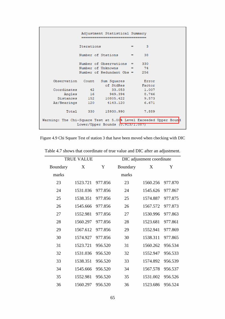
Figure 4.9 Chi Square Test of station 3 that have been moved when checking with DIC
Table 4.7 shows that coordinate of true value and DIC after an adjustment.
TRUE VALUE DIC adjustment coordinate
Boundary
marks
X Y Boundary
marks
X Y
23 1523.721 977.856 23 1560.256 977.870
24 1531.036 977.856 24 1545.626 977.867
25 1538.351 977.856 25 1574.887 977.875
26 1545.666 977.856 26 1567.572 977.873
27 1552.981 977.856 27 1530.996 977.863
28 1560.297 977.856 28 1523.681 977.861
29 1567.612 977.856 29 1552.941 977.869
30 1574.927 977.856 30 1538.311 977.865
31 1523.721 956.520 31 1560.262 956.534
32 1531.036 956.520 32 1552.947 956.533
33 1538.351 956.520 33 1574.892 956.539
34 1545.666 956.520 34 1567.578 956.537
35 1552.981 956.520 35 1531.002 956.526
36 1560.297 956.520 36 1523.686 956.524
66
37 1567.612 956.520 37 1545.632 956.531
38 1574.927 956.520 38 1538.318 956.529
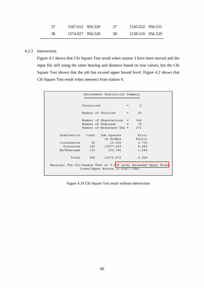
4.2.3 Intersection
Figure 4.1 shows that Chi Square Test result when station 3 have been moved and the
input file still using the same bearing and distance based on true values, but the Chi
Square Test shown that the job has exceed upper bound level. Figure 4.2 shows that
Chi Square Test result when intersect from station 4.
Figure 4.10 Chi Square Test result without intersection
67
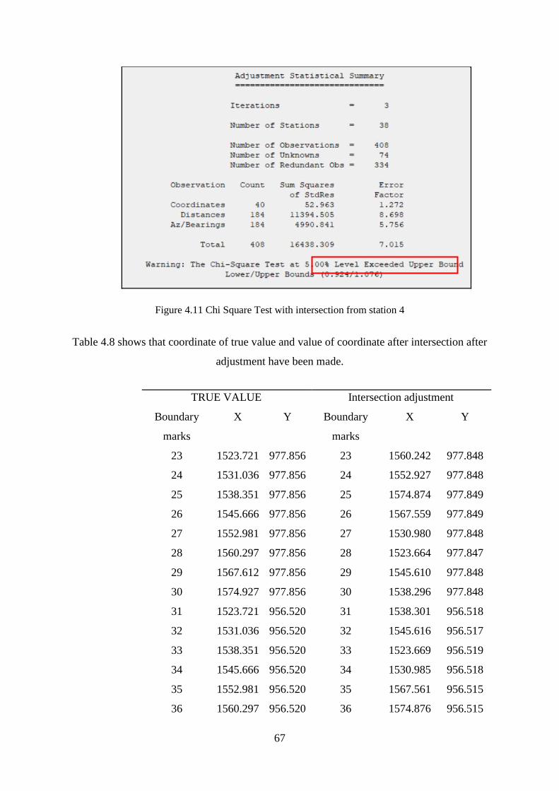
Figure 4.11 Chi Square Test with intersection from station 4
Table 4.8 shows that coordinate of true value and value of coordinate after intersection after
adjustment have been made.
TRUE VALUE Intersection adjustment
Boundary
marks
X Y Boundary
marks
X Y
23 1523.721 977.856 23 1560.242 977.848
24 1531.036 977.856 24 1552.927 977.848
25 1538.351 977.856 25 1574.874 977.849
26 1545.666 977.856 26 1567.559 977.849
27 1552.981 977.856 27 1530.980 977.848
28 1560.297 977.856 28 1523.664 977.847
29 1567.612 977.856 29 1545.610 977.848
30 1574.927 977.856 30 1538.296 977.848
31 1523.721 956.520 31 1538.301 956.518
32 1531.036 956.520 32 1545.616 956.517
33 1538.351 956.520 33 1523.669 956.519
34 1545.666 956.520 34 1530.985 956.518
35 1552.981 956.520 35 1567.561 956.515
36 1560.297 956.520 36 1574.876 956.515
68
4.3 Analysis and Discussion
4.3.1 Residual bearing, distance and area of radiate method
From the Table 4.1 above shows that value of residual bearing, residual distance and
residual area that has been radiate 50m from control points. The mean for distance is
00-00-03. The minimum value of residual bearing is – 00-00-18 after been adjusted in
STAR*Net and maximum value of residual bearing is 00-00-23. The range for this
residual after is 00-00-41. The standard deviation for 50 meters radiated is 00-00-12.
As for residual distance, the mean is 0.000, minimum value is -0.002m, and maximum
value is 0.002m. Range of this residual distance is 0.004m. The standard deviation
distance for 50 meters radiate is 0.001m. As for residual area, the mean of this residual
shows that -0.001𝑚2, the minimum value is -0.026𝑚2, the maximum value is 0.023𝑚2.
The range for this area after been adjusted in STAR*Net is 0.049𝑚2. The standard
deviation for this is 0.015𝑚2.
The result of radiate from distance 100m shows that mean of residual bearing are
00°00′02" with minimum residual bearing after been adjusted is − 00°01′05" and
maximum residual bearing 00°01′14". The range for residual bearing shows that
− 00°02′29"between minimum and maximum residual bearing. The standard deviation
for 100m radiate is − 00°00′33". The average of residual distance for 100m radiate is
0.000m. The minimum value after being adjusted using LSA for 100m radiate is -
0.004m and maximum residual distance is 0.003m. The range of residual distance is
0.007m and the standard deviation for distance radiate from 100m is 0.002m. As for
residual area, the mean of this residual shows that average of 100m is -0.005𝑚2. The
minimum of residual area is -0.025𝑚2, maximum of residual area is 0.006𝑚2 and range
between residual area is 0.031𝑚2. The standard deviation area from 100m radiate is
0.012𝑚2.
37 1567.612 956.520 37 1552.9312 956.5160
38 1574.927 956.520 38 1560.2461 956.5151
69
The result of radiate from distance 150m shows that mean of residual bearing are
00°00′03" with minimum value of residual bearing after been adjusted is
− 00°01′10" and maximum residual bearing 00°01′13". The range for residual bearing
shows that − 00°02′23" between minimum and maximum residual bearing. The
standard deviation for 100m radiate is − 00°00′35". This show increasing value when
radiate far from control points. The average of residual distance for 150m radiate is
0.000m. The minimum value after being adjusted using LSA for 100m radiate is -
0.001m and maximum residual distance is 0.00m. The range of residual distance is
0.004m and the standard deviation for distance radiate from 100m is 0.001m. As for
residual area, the mean of this residual shows that average of 100m is 0.006𝑚2. The
minimum value of residual area is -0.008𝑚2, maximum of residual area is 0.031𝑚2 and
range between residual area is 0.039𝑚2. The standard deviation area from 150m radiate
is 0.013𝑚2.
The result of radiate from distance 200m shows that mean of residual bearing are
00°00′50" with minimum residual bearing after been adjusted is − 00°01′07" and
maximum residual bearing 00°00′52". The range for residual bearing show that
− 00°01′59"between minimum and maximum residual bearing. The standard deviation
for 100m radiate is − 00°00′33". The average of residual distance for 100m radiate is
0.000m. The minimum value after being adjusted using LSA for 100m radiate is -
0.003m and maximum residual distance is 0.002m. The range of residual distance is
0.005m and the standard deviation for distance radiate from 200m is 0.001m. As for
residual area, the mean of this residual shows that average of 200m is 0.004𝑚2. The
minimum value of residual area is -0.029𝑚2, maximum of residual area is 0.029𝑚2 and
range between residual area is 0.058𝑚2. The standard deviation area from 200m radiate
is 0.020𝑚2.
The result of radiate from distance 250m shows that mean of residual bearing is -
00°00'06" with minimum residual bearing after been adjusted is -00°01'56" and
maximum residual bearing 00°02'41". The range for residual bearing shows that -
00°04'37"between minimum and maximum residual bearing. The standard deviation
for 250m radiate is 00°00'51". This is the highest standard deviation among others
radiation distance. The average of residual distance for 250m radiate is 0.000m. The
70
minimum value after being adjusted using LSA for 250m radiate is -0.003m and
maximum residual distance is 0.004m. The range of residual distance is 0.007m and the
standard deviation for distance radiate from 100m is 0.002m. As for residual area, the
mean of this residual shows that average of 250m is -0.003𝑚2. The minimum of
residual area is -0.043𝑚2, maximum of residual area is 0.014𝑚2 and range between
residual area is 0.057𝑚2. The standard deviation area from 250m radiate is 0.020𝑚2.
The result of radiate from distance 3000m shows that mean of residual bearing is
00°00'09" with minimum residual bearing after been adjusted is -00°01'32" and
maximum residual bearing 00°01'14". The range for residual bearing shows that -
00°02'46"between minimum and maximum residual bearing. The standard deviation
for 300m radiate is 00°00'43". This is the one of the highest standard deviation among
others radiation distance. The average of residual distance for 300m radiate is 0.001m.
The minimum value after being adjusted using LSA for 300m radiate is -0.009m and
maximum residual distance is 0.008m. The range of residual distance is 0.017m and the
standard deviation for distance radiate from 300m is 0.003m. As for residual area, the
mean of this residual shows that average of 300m is 0.027𝑚2. The minimum of residual
area is -0.093𝑚2., maximum of residual area is 0.056𝑚2. and range between residual
area is 0.149𝑚2. The standard deviation area from 300m radiate is 0.053𝑚2.
The result from table shows that the increasing value in mean, minimum, maximum,
range and standard deviation after radiated from near and to far control points. A low
standard deviation show that the data points tend to be close to the mean while a high
standard deviation show that the data points are distributed over a wide range of values.
In this case it is clearly indicates that the increasing value of the standard deviation
shows that using radiate method far from the control points is not appropriately used
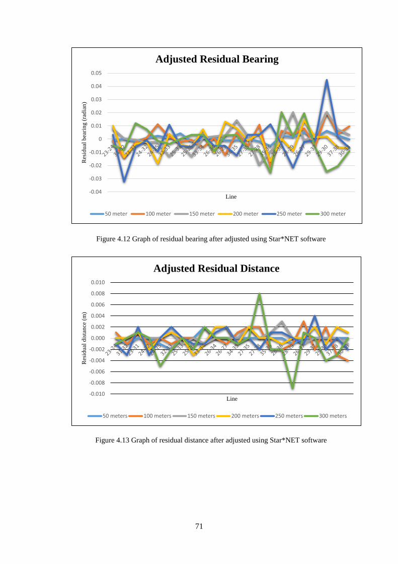
for setting out the terrace house in least square adjustment environment. Figure 4.12,
Figure 4.13 and figure 4.14 shows that residual graph in bearing, distance and area.
71
Figure 4.12 Graph of residual bearing after adjusted using Star*NET software
Figure 4.13 Graph of residual distance after adjusted using Star*NET software
-0.04
-0.03
-0.02
-0.01
0
0.01
0.02
0.03
0.04
0.05
Res
idu
al b
eari
ng (
rad
ian
)
Line
Adjusted Residual Bearing
50 meter 100 meter 150 meter 200 meter 250 meter 300 meter
-0.010
-0.008
-0.006
-0.004
-0.002
0.000
0.002
0.004
0.006
0.008
0.010
Res
idu
al d
ista
nce
(m
)
Line
Adjusted Residual Distance
50 meters 100 meters 150 meters 200 meters 250 meters 300 meters
72
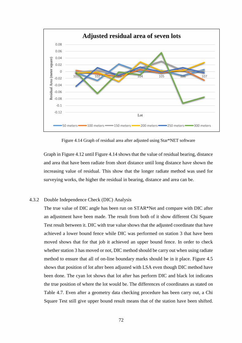
Figure 4.14 Graph of residual area after adjusted using Star*NET software
Graph in Figure 4.12 until Figure 4.14 shows that the value of residual bearing, distance
and area that have been radiate from short distance until long distance have shown the
increasing value of residual. This show that the longer radiate method was used for
surveying works, the higher the residual in bearing, distance and area can be.
4.3.2 Double Independence Check (DIC) Analysis
The true value of DIC angle has been run on STAR*Net and compare with DIC after
an adjustment have been made. The result from both of it show different Chi Square
Test result between it. DIC with true value shows that the adjusted coordinate that have
achieved a lower bound fence while DIC was performed on station 3 that have been
moved shows that for that job it achieved an upper bound fence. In order to check
whether station 3 has moved or not, DIC method should be carry out when using radiate
method to ensure that all of on-line boundary marks should be in it place. Figure 4.5
shows that position of lot after been adjusted with LSA even though DIC method have
been done. The cyan lot shows that lot after has perform DIC and black lot indicates
the true position of where the lot would be. The differences of coordinates as stated on
Table 4.7. Even after a geometry data checking procedure has been carry out, a Chi
Square Test still give upper bound result means that of the station have been shifted.
-0.12
-0.1
-0.08
-0.06
-0.04
-0.02
0
0.02
0.04
0.06
0.08
101 102 103 104 105 106 107
Res
idu
al A
rea
(met
er s
qu
are)
Lot
Adjusted residual area of seven lots
50 meters 100 meters 150 meters 200 meters 250 meters 300 meters

73
Figure 4.6 shows that listing error from STAR*Net software shows that standard
residual of line 3-4 after been adjusted.
Figure 4.15 Cyan lot indicate to the position of lot after station have been moved
Figure 4.16 Listing error from STAR*Net software
4.3.3 Intersection Method Analysis
A geometry data checking using intersection have conduct between station 3 that have
shift and station 4. In order to ensure either station 3 have shift or not, intersection
method was used. Figure 4.6 shows that adjusted distance for line 3-4 and standard
residual shows that a high error on that line. The STAR*Net software shows that on
that particular line have error either that station has been shift or gross error have occurs
during input data process. But for this case, all the gross error has been removed yet
still get an upper bound fence.

74
Figure 4.17 Listing error from STAR*Net

75
CHAPTER FIVE
CONCLUSION
To sum up this research this research has achieved its aim which are on how to
apply the radiation method in on-line method in Least Square Adjustment
environment. In order to make the successfulness of this study, three objectives
have been set to achieved aim for this study. The first objective is to study the
impact of on-line method based on single leg which is radiate method. Six distance
have radiated from several control points to the terrace house from short distance
to long distance from the control points. To result after adjustment shows that the
different value between true value in terms of bearing, distance and area. A residual
has been calculated using IBM SPSS Statistic software to calculate the mean,
minimum, maximum, range and standard deviation for six distance. As the result
shows that the longer distance has been radiate from control points, the increasing
value of mean, minimum, maximum, range and standard deviation. The standard
deviation for this study is a guideline when performing radiate method on field
work, based on certain distance, the tolerance when radiate from short to long
distance should be in tolerance as stated in Table 4.1 until Table 4.6
The second objective is to study the on-line method based on geometry data
checking using double independent check (DIC) and intersection method. In order
to apply the geometry data checking, one of the stations has been shifted to
demonstrate the crucial of geometry data checking during on-line work. Even
during field work surveyor set the true bearing but if the surveyor observed from
the shifted station, all of the terrace house coordinates have been emplace on the
wrong location. In order to prevent this from happening, a geometry data checking
should be practice when performing radiate method in on-line work.

76
The third objective is to propose the new suggestion method procedure of geometry
data checking during emplace boundary marks. This third objective is relating to
the second objective. This geometry data checking should be proposed to the
Department Survey and Mapping Malaysia resulting from the second objective
from preventing all of the wrongly coordinate have been inserted to database.
REFERENCES
Abdul Halim, N. Z., Sulaiman, S. A., Talib, K., & Majeed, Z. A. (2018). Investigating the
national digital cadastral database (NDCDB) data handling within GIS applications.
International Archives of the Photogrammetry, Remote Sensing and Spatial
Information Sciences - ISPRS Archives, 42(4/W9), 3–10.
https://doi.org/10.5194/isprs-archives-XLII-4-W9-3-2018
Bird, R. G. (1972). Least squares adjustment of E.D.M. traverses. Survey Review, 21(165),
307–319. https://doi.org/10.1179/sre.1972.21.165.307
Chen, Q., Chen, H., Jiang, W., Zhou, X., & Yuan, P. (2018). A New Cycle Slip Detection
and Repair Method for Single-Frequency GNSS Data. Journal of Navigation, 71(6),
1492–1510. https://doi.org/10.1017/S0373463318000243
Fiadeiro, P. (1987). Calculation of Exact Position Using Intersection, Resection and
Distances with Least Squares Adjustment. International Hydrographic Review, 64(1).
Font-Llagunes, J. M., & Batlle, J. A. (2009). New method that solves the three-point
resection problem using straight lines intersection. Journal of Surveying Engineering,
135(2), 39–45. https://doi.org/10.1061/(ASCE)0733-9453(2009)135:2(39)
Fu, W., Huang, G., Zhang, Q., Gu, S., Ge, M., & Schuh, H. (2019). Multi-GNSS real-time
clock estimation using sequential least square adjustment with online quality control.
Journal of Geodesy, 93(7), 963–976. https://doi.org/10.1007/s00190-018-1218-z
Ghilani, C., & Wolf, P. (2006). Adjustment computations: spatial data analysis. In
International Journal of Geographical Information Science (Fourth Edi, Vol. 25).
https://doi.org/10.1080/13658816.2010.501335
Halim, N. Z.A., Sulaiman, S. A., Talib, K., & Ng, E. G. (2018). Identifying the relevant
features of the National Digital Cadastral Database (NDCDB) for spatial analysis by
using the Delphi Technique. IOP Conference Series: Earth and Environmental
Science, 117(1). https://doi.org/10.1088/1755-1315/117/1/012030
Halim, Nur Zurairah Abdul, Sulaiman, S. A. H., Talib, K. H., Yusof, O. M., Wazir, M. A.
M., & Adimin, H. M. K. (2017). Legal significance of National Digital Cadastral
Database (NDCDB) in Malaysia cadastral system. 2017 IEEE 8th Control and System
Graduate Research Colloquium, ICSGRC 2017 - Proceedings, (August), 179–184.
https://doi.org/10.1109/ICSGRC.2017.8070591
Jeffri, M., Hisham, O., & Joanes, J. (2017). EFFECTIVENESS OF LOCALISED
ADJUSTMENT IN STRENGTENING NATIONAL DIGITAL CADASTRE
DATABASE. Jurnal Teknologi. Retrieved from www.jurnalteknologi.utm.my
Kadir, M., Ses, S., Desa, G., Tong, C. W., & Boo, T. C. (2000). Towards the
implementation of coordinated cadastral system in Malaysia : Large cadastral network
adjustments. Australian Surveyor, 45(1), 37–46.
https://doi.org/10.1080/00050326.2000.10441932
Leahy, F. J. (1977). Bowditch revisited. Australian Surveyor, 28(8), 475–487.
https://doi.org/10.1080/00050326.1977.10441442
Rajabifard, A., Agunbiade, M., Kalantari, M., Yip, K. M., Atazadeh, B., Badiee, F., …
Anaraki, M. R. (2018). An LADM-based Approach for Developing and Implementing
a National 3D Cadastre – A Case Study of Malaysia. Researchgate-Online, (April),
47–66. Retrieved from
https://wiki.tudelft.nl/pub/Research/ISO19152/LADM2018Workshop/04-
18_LADM_2018.pdf
Teoh, C. H. (2009). An integrated GIS database server for Malaysian mapping, cadastral
and location-based systems (LBS). 2009 WRI World Congress on Computer Science
and Information Engineering, CSIE 2009, 4, 162–167.
https://doi.org/10.1109/CSIE.2009.938
Walker, J., & Awange, J. L. (2018). Surveying for Civil and Mine Engineers: Theory,
Workshops, and Practicals. In Surveying for Civil and Mine Engineers.
https://doi.org/10.1007/978-3-319-53129-8
Yunus, M., Yusoff, M., Jamil, H., Zurairah, N., & Halim, A. (2013). eKadaster : A
Learning Experience for Malaysia Ekadaster : A Learning Experience for Malaysia.
FIG Pacific Small Island Developing States Symposium, Suva, Fiji 18-20 September
2013, 18–20.
Pekeliling Ketua Pengarah Ukur dan Pemetaan Bilangan 6 Tahun 2009.
National Land Code (Act 56 of 1965) and Regulations.

APPENDIX
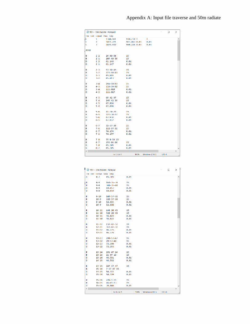
Appendix A: Input file traverse and 50m radiate
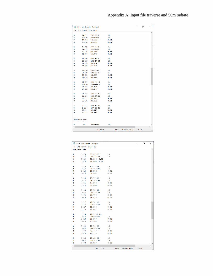
Appendix A: Input file traverse and 50m radiate
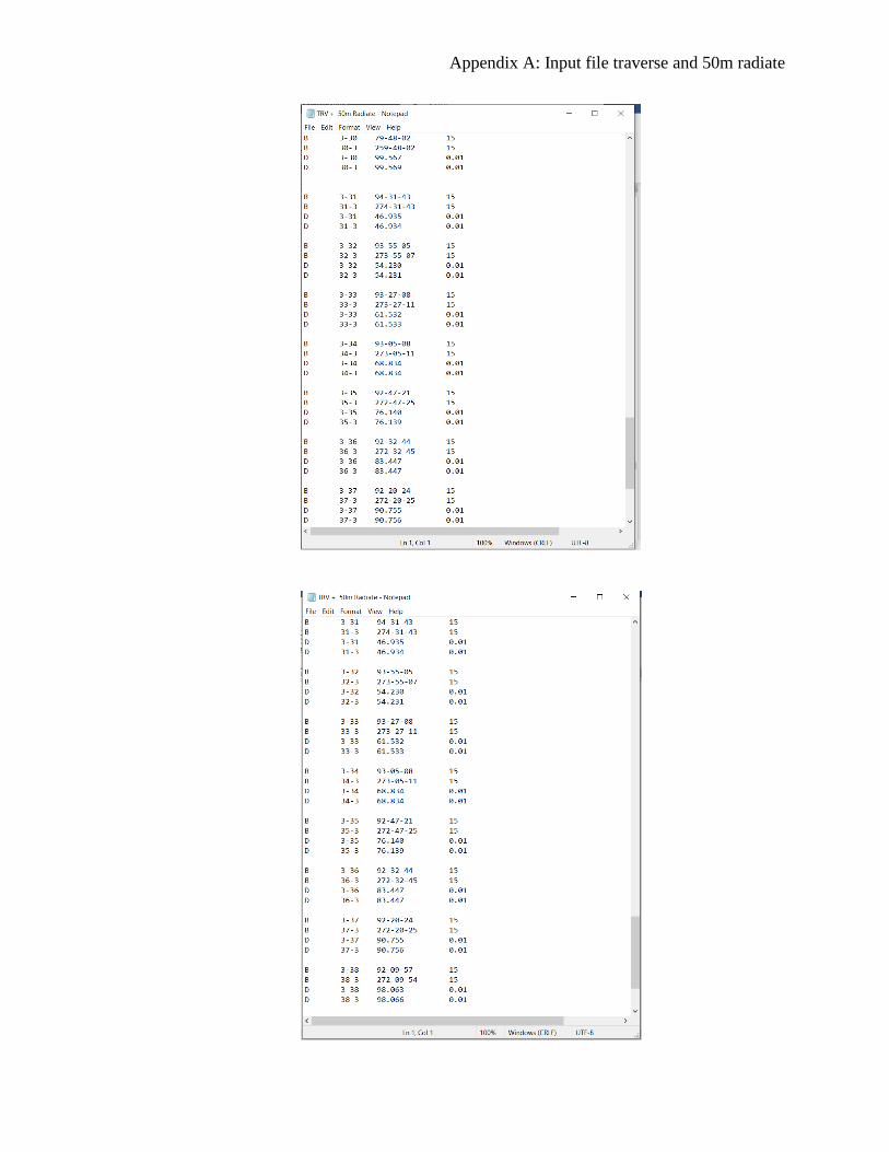
Appendix A: Input file traverse and 50m radiate
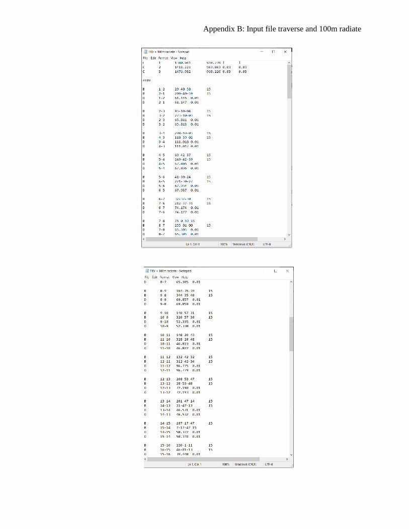
Appendix B: Input file traverse and 100m radiate
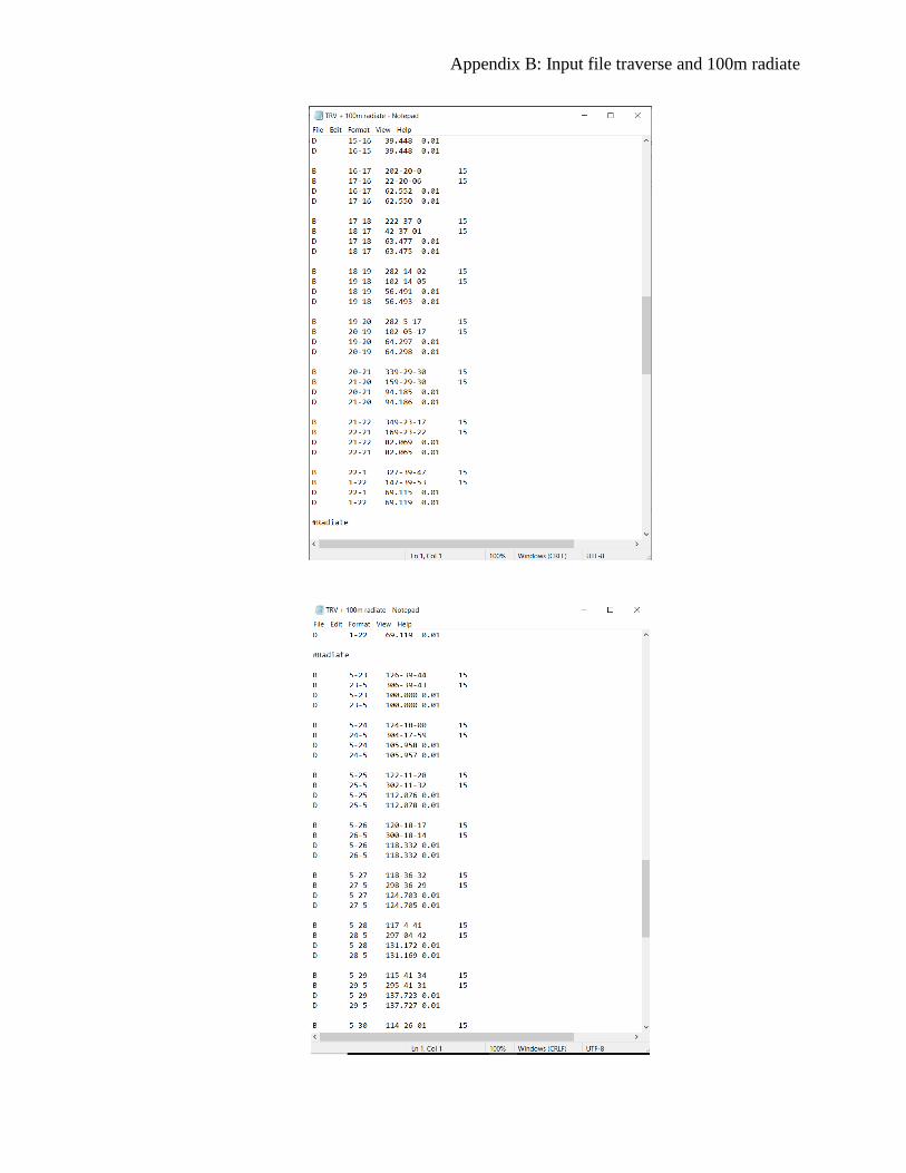
Appendix B: Input file traverse and 100m radiate
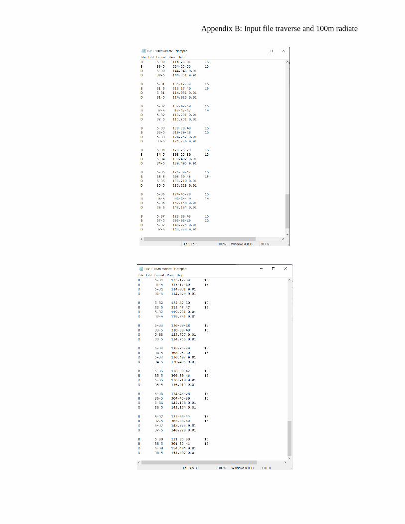
Appendix B: Input file traverse and 100m radiate
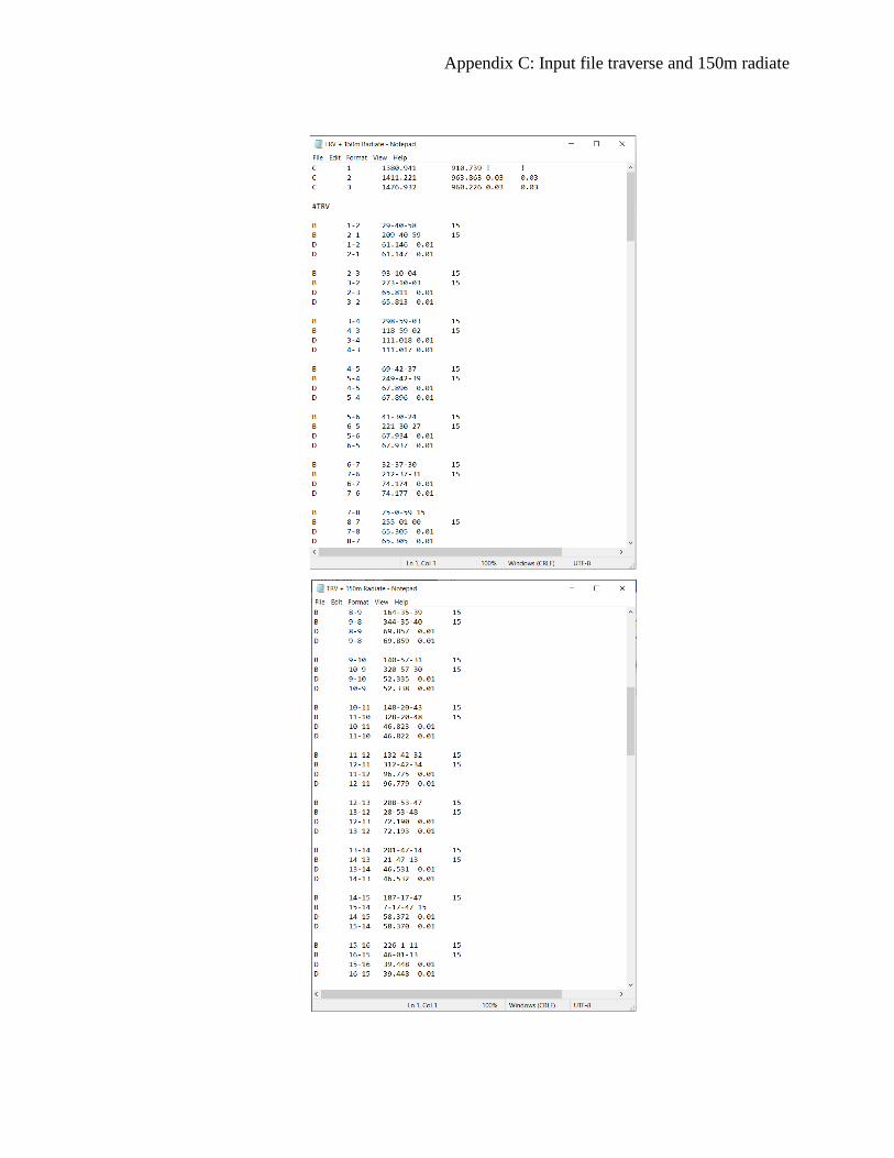
Appendix C: Input file traverse and 150m radiate
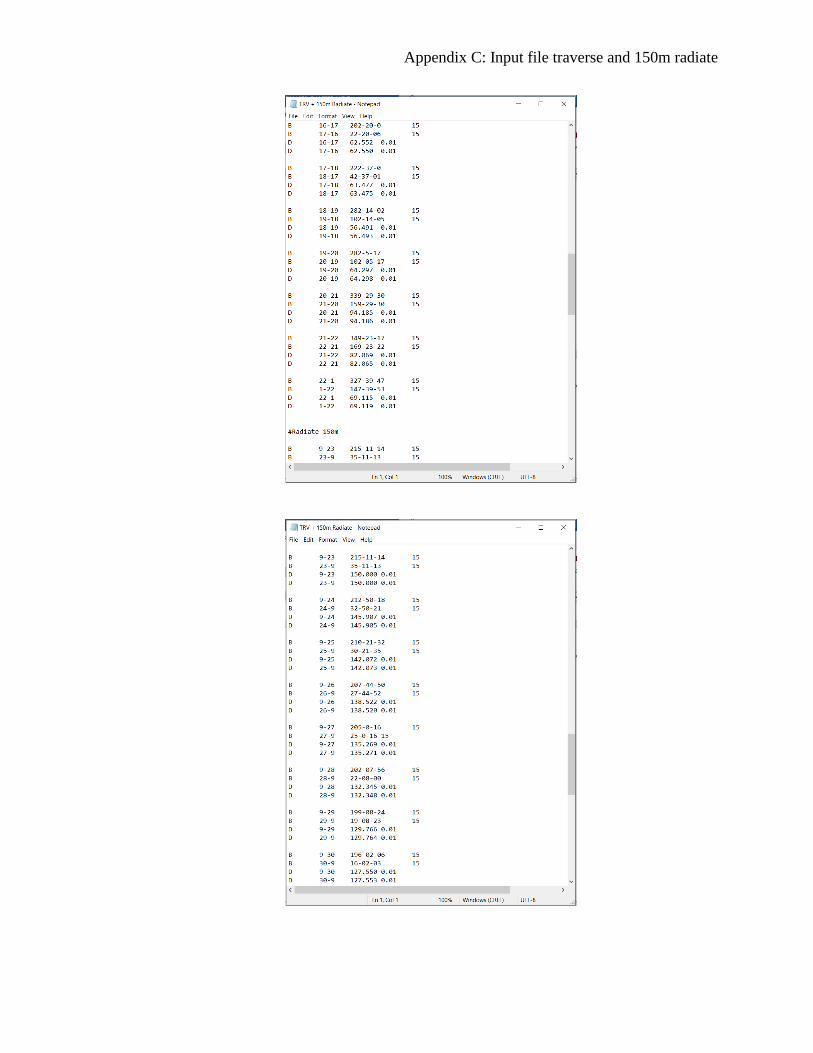
Appendix C: Input file traverse and 150m radiate
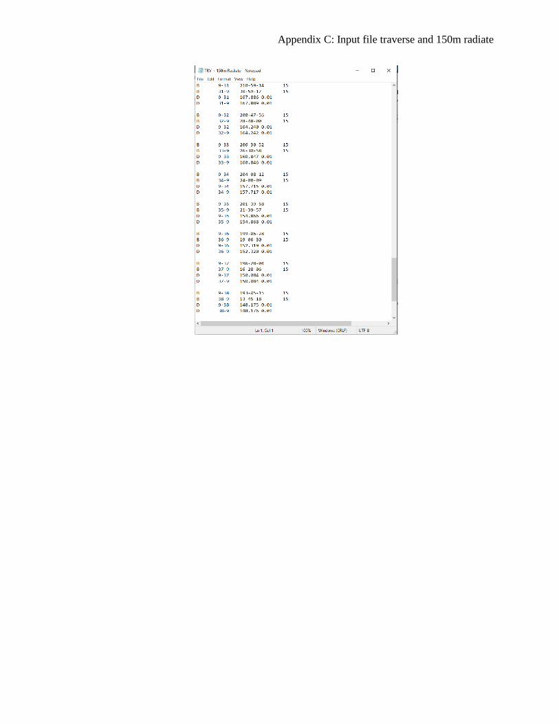
Appendix C: Input file traverse and 150m radiate

Appendix D: Input file traverse and 200m radiate

Appendix D: Input file traverse and 200m radiate
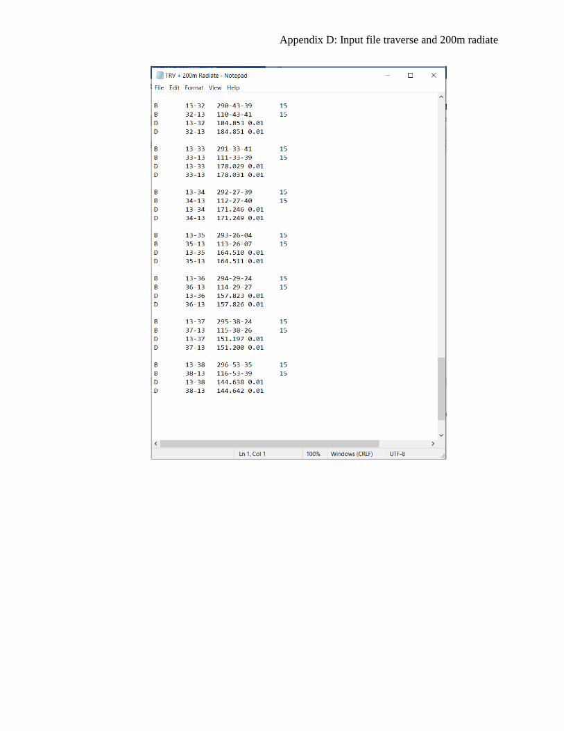
Appendix D: Input file traverse and 200m radiate
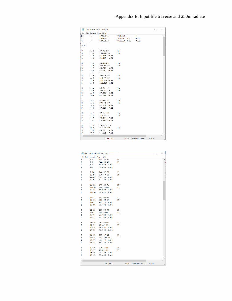
Appendix E: Input file traverse and 250m radiate

Appendix E: Input file traverse and 250m radiate
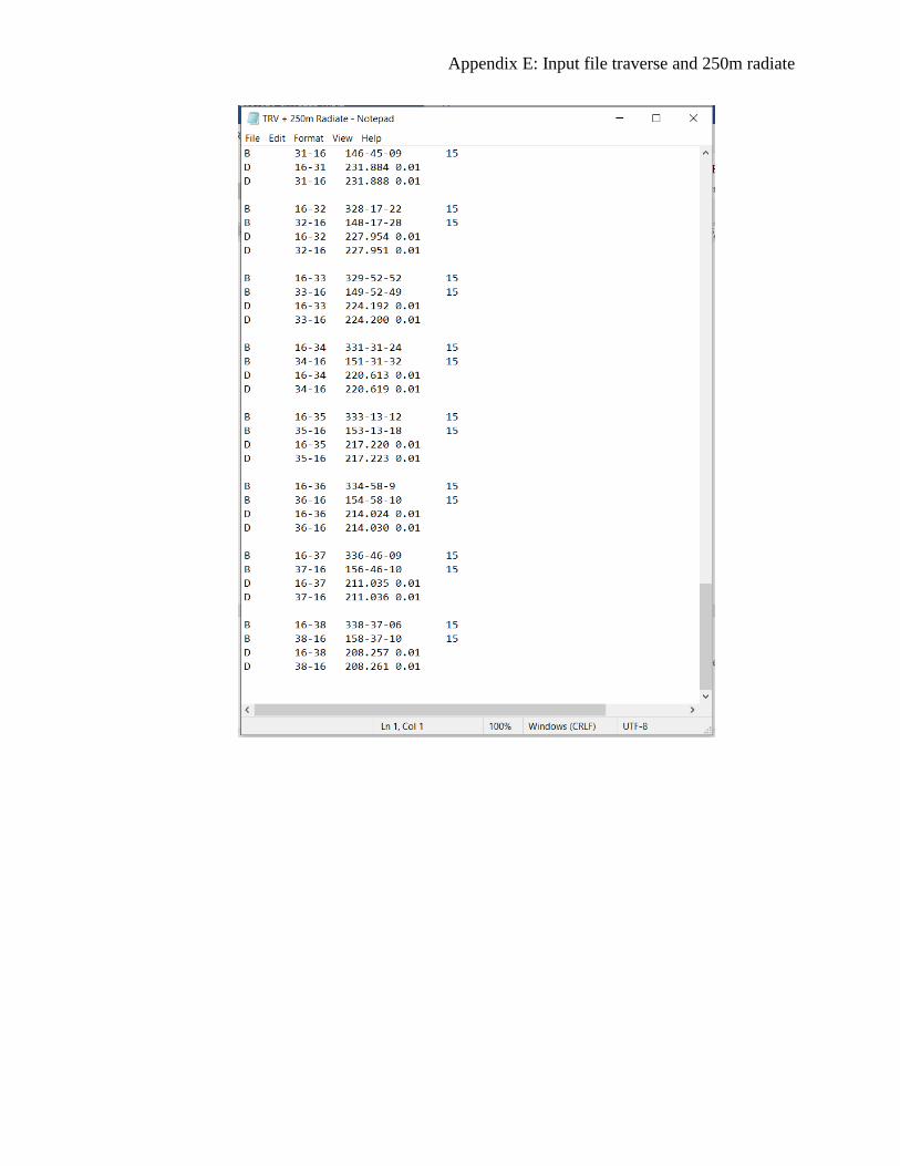
Appendix E: Input file traverse and 250m radiate
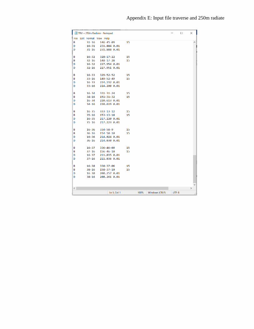
Appendix E: Input file traverse and 250m radiate
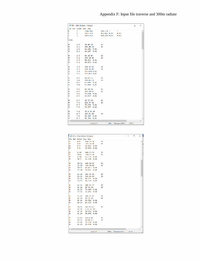
Appendix F: Input file traverse and 300m radiate
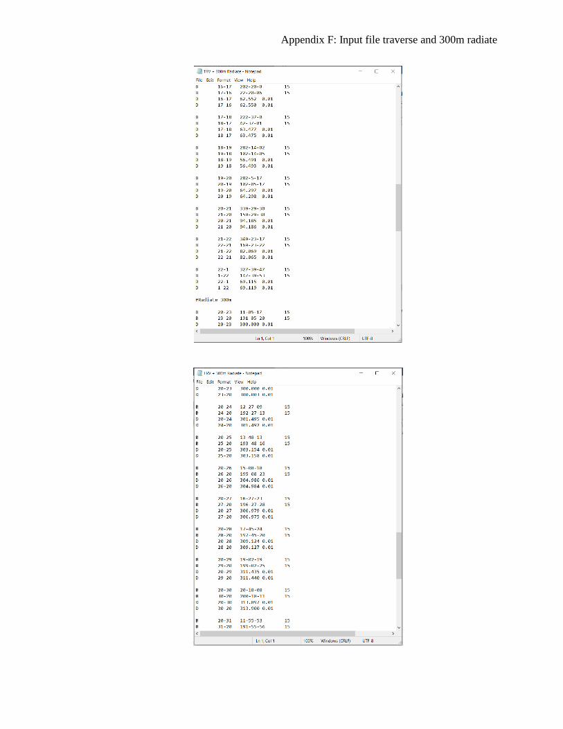
Appendix F: Input file traverse and 300m radiate
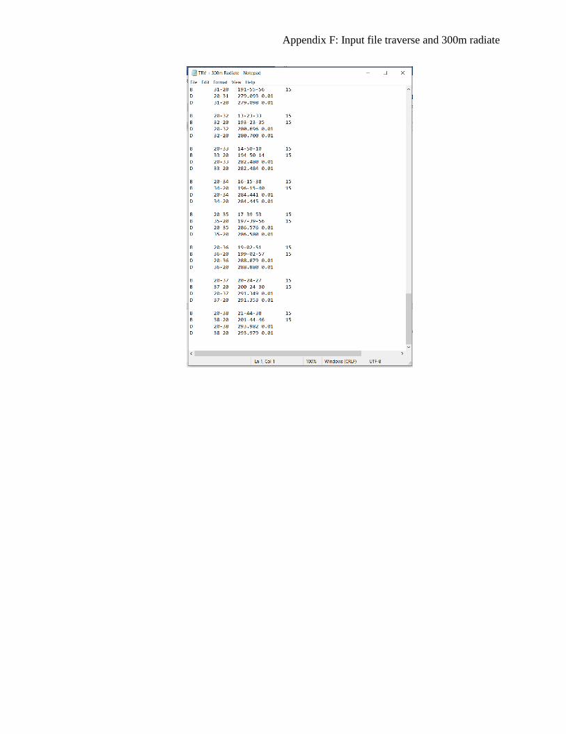
Appendix F: Input file traverse and 300m radiate
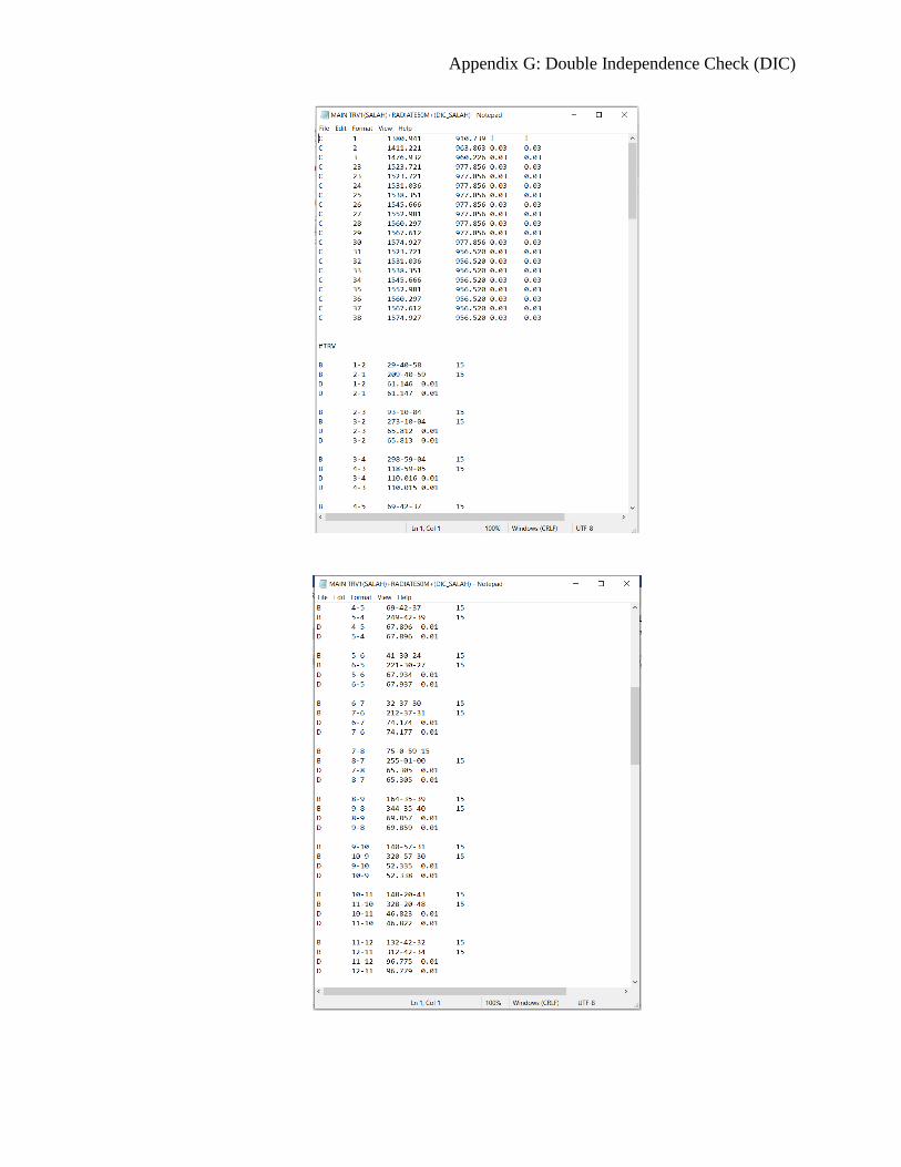
Appendix G: Double Independence Check (DIC)

Appendix G: Double Independence Check (DIC)
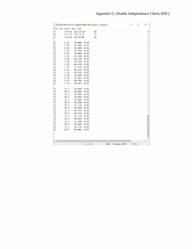
Appendix G: Double Independence Check (DIC)
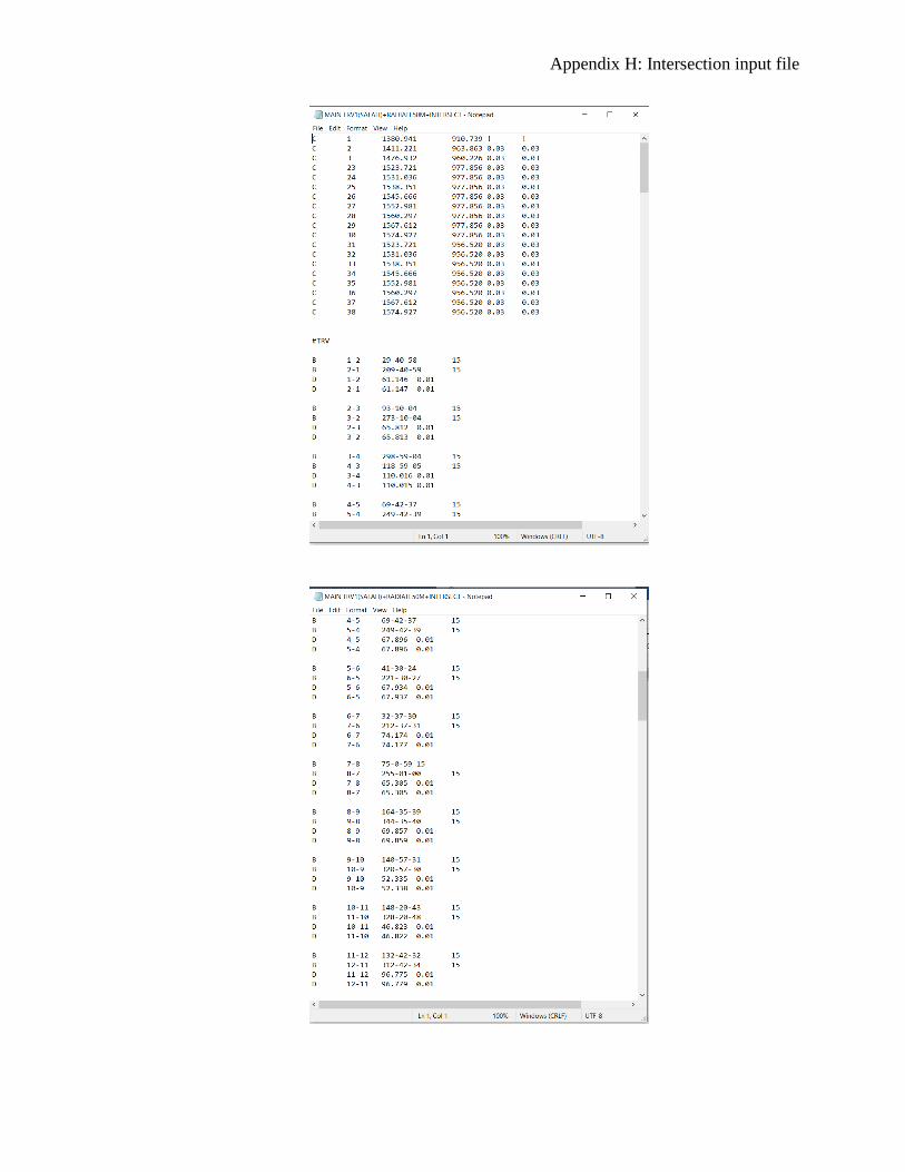
Appendix H: Intersection input file
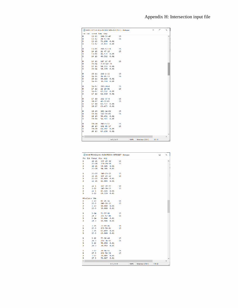
Appendix H: Intersection input file
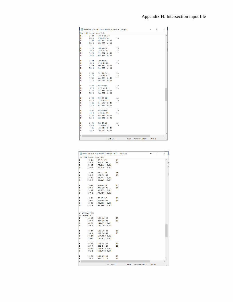
Appendix H: Intersection input file
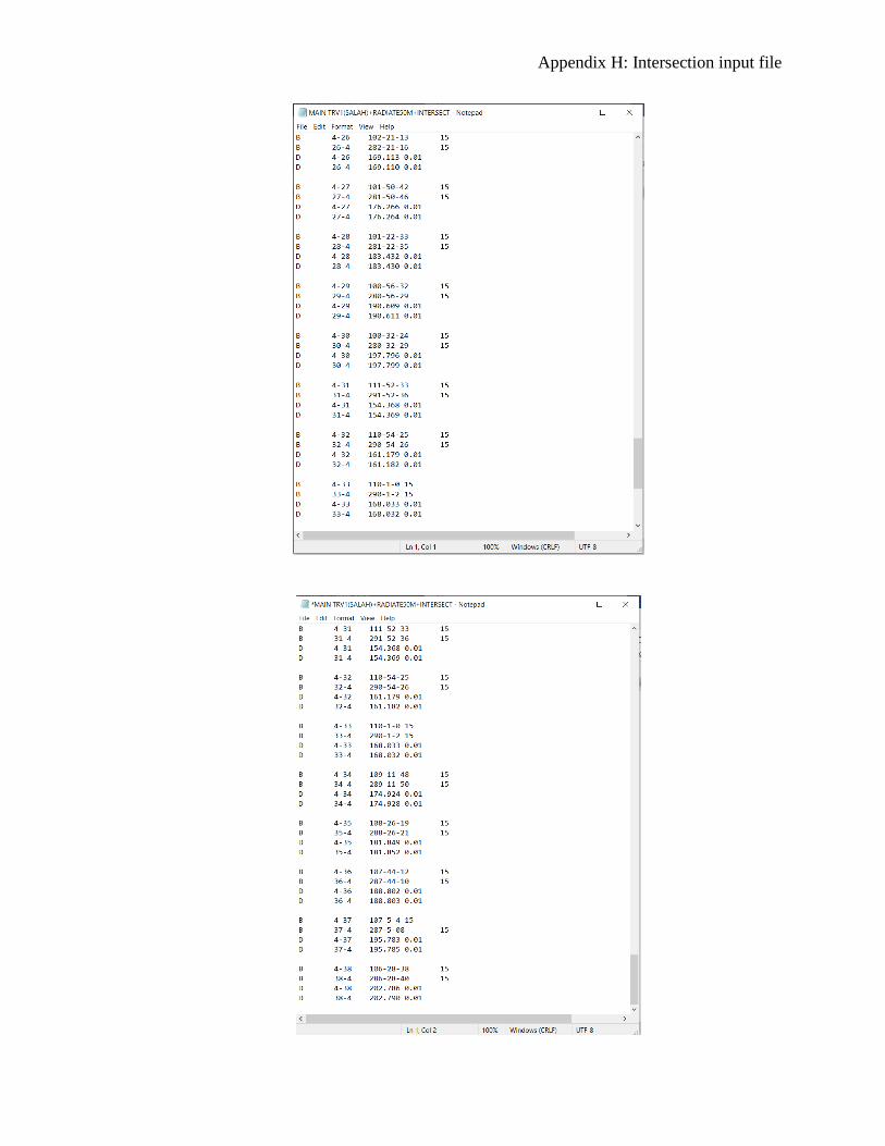
Appendix H: Intersection input file