Embed Size (px)
Citation preview
University Institute of Lisbon
Department of Finance
Credit VaR and VaR in Credit Default Swaps
Sofia Bernardo Rodrigues
A Thesis presented in partial fulfillment of the Requirements for the Degree of Doctor
Supervisor:
Joao Pedro Pereira, Assistant Professor,
ISCTE - University Institute of Lisbon,
December, 2013

University Institute of Lisbon
Department of Finance
Credit VaR and VaR in Credit Default Swaps
Sofia Bernardo Rodrigues
A Thesis presented in partial fulfillment of the Requirements for the Degree of Doctor
Jury:
Doctor Maria Isabel Fraga Alves, Associate Professor, Faculdade de Ciencias -
Universidade de Lisboa
Doctor Paulo Manuel Marques Rodrigues, Adjunct Associate Professor, Nova School
of Business and Economics - Universidade Nova de Lisboa
Doctor Jorge Barros Luıs, Adjunct Assistant Professor, ISEG - Lisbon School of
Economics and Management - Universidade de Lisboa
Doctor Luıs Filipe Sousa Martins, Assistant Professor, ISCTE - University Institute of
Lisbon
Doctor Joao Pedro Pereira, Assistant Professor, ISCTE - University Institute of Lisbon
December, 2013


Resumo
Nesta tese sao apresentadas duas aplicacoes de estimacao de Value at Risk (VaR): VaR
de Credito e VaR em Credit Default Swaps (CDS).
O VaR de credito foi estimado com base em pressupostos de correlacao diferentes,
utilizando as copulas Gaussiana e t, e comparado com a perda observada numa car-
teira de credito de uma instituicao financeira Portuguesa, num total de 72 observacoes
mensais no perıodo entre 2004 e 2009. Concluo que existe evidencia empırica de que
algumas das hipoteses assumidas pelas agencias de rating para avaliar CDOs sao de-
sadequadas em situacoes de stress, como a crise financeira observada em 2008. As
estimativas de VaR de credito foram comparadas usando procedimentos de backtesting.
O modelo que melhor se adequa ao portfolio em analise baseia-se no estimador empırico
de correlacao proposto por De Servigny e Renault (2002a), considerando a copula t com
8 graus de liberdade.
Relativamente a aplicacao de modelos de VaR a CDS, o VaR foi estimado usando
varios metodos: Regressao de Quantis, Simulacao Historica, Simulacao Historica Fil-
trada, Teoria dos Valores Extremos e varios modelos GARCH. A analise baseia-se em
242 entidades, no perıodo entre setembro 2001 e abril 2011. As estimativas de VaR
em CDS foram comparadas usando procedimentos de backtesting. Concluo que a Re-
gressao de Quantis proporciona melhores resultados na estimacao de VaR que os res-
tantes metodos e que os racios financeiros propostos por Campbell et al (2008) para
determinar o risco de falencia contribuem para explicar o preco do CDS.
Palavras-Chave: Value at Risk, Copulas, Correlacao, Regressao de Quantis
Classificacao JEL: C01, C02

Abstract
This thesis presents two applications of Value at Risk (VaR) estimation: Credit VaR and
VaR in Credit Default Swaps (CDS).
I compare Credit VaR estimates based on different correlation assumptions, using
Gaussian and t copulas, with the observed loss in a credit portfolio of a Portuguese fi-
nancial institution, for a time series of 72 monthly observations, covering the period
between 2004 and 2009. I provide empirical evidence that some of the assumptions
made by rating agencies to evaluate CDOs are inadequate in stress situations like the
financial crisis observed in 2008. All Credit VaR estimates were compared using back-
testing procedures. I find that the most accurate Credit VaR model for this portfolio is
based on asset correlation given by the empirical estimator proposed by De Servigny
and Renault (2002a) and assuming a dependence structure given by the t copula with 8
degrees of freedom.
Regarding the application of VaR models to CDS, I estimate VaR using several
methods: Quantile Regression, Historical Simulation, Filtered Historical Simulation,
Extreme Value Theory and GARCH-based models. The analysis of the determinants of
CDS spreads is based on 242 reference entities and the time period ranges from Septem-
ber 2001 to April 2011. All VaR models were compared using backtesting procedures.
I find that Quantile Regression provides better results than the other models tested and
that the financial ratios proposed by Campbell et al (2008) to determine the risk of
bankruptcy contribute to explain the determinants of the price of CDS.
Keywords: Value at Risk, Copulas, Correlation, Quantile Regression
JEL Classification: C01, C02

Executive Summary
This thesis presents two applications of Value at Risk (VaR) estimation: Credit VaR and
VaR in Credit Default Swaps (CDS).
Value at Risk estimates of credit portfolios depend on default probability, recovery
rate and asset correlation. Previous literature has pointed asset correlation as one of
the major weaknesses of VaR estimates and a factor that played a major role in the fi-
nancial crisis observed in 2008. Rating agencies faced heavy criticism regarding the
assumptions used to evaluate Collateralized Debt Obligations but there is few empirical
evidence to support that criticism. One of the goals of this study is to compare differ-
ent approaches to calculate credit VaR with the loss observed in a financial institution
portfolio and analyze the sensitivity of VaR estimates to different assumptions regarding
asset correlation.
I compare Credit VaR estimates based on different correlation assumptions, using
Gaussian and t copulas, with the observed loss in a credit portfolio of a Portuguese fi-
nancial institution, for a time series of 72 monthly observations, covering the period
between 2004 and 2009. I find that credit VaR estimates differ substantially, depending
on the assumptions regarding asset correlation and dependence structure. This finding
reinforces the crucial role that the assumption regarding correlation plays in credit VaR
estimation. I also provide empirical evidence that some of the assumptions made by ma-
jor rating agencies to evaluate CDOs are inadequate in stress situations like the financial
crisis observed in 2008. I find that the more accurate VaR model for the portfolio used in
this study is based on asset correlation given by the empirical estimator of De Servigny
and Renault (2002a) and assuming t copula with 8 degrees of freedom.
Credit Default Swaps were at the forefront of the recent financial crisis of 2007-2009
and many observers have blamed CDS as one of the lead causes of the crisis. However,
a more careful analysis, as done in Stulz (2009), suggests that CDS did not trigger the
crisis and that in fact they allowed some institutions to limit their losses and, for this
reason, CDS are certain to remain a crucial financial instrument, even though under
tighter regulation and more control.
Regarding the application of VaR models to CDS, the goal of this study is to estimate
VaR in CDS using Quantile Regression, covering the period of the recent financial crisis,
and perform a thorough evaluation of VaR estimates and compare them with alternative
methods, namely Historical Simulation, Filtered Historical Simulation, Extreme Value
Theory and GARCH-based models, through backtesting methodologies. The analysis
of the determinants of CDS spreads is based on 242 reference entities and the time
period ranges from September 2001 to April 2011. I find that Quantile Regression pro-
vides better results than the other models tested and that the financial ratios proposed
by Campbell et al (2008) to determine the risk of bankruptcy contribute to explain the
determinants of the price of CDS.

Acknowledgements
I am deeply grateful to my advisor Professor Joao Pedro Pereira for all his encourage-
ment, support and guidance.
Financial support from bank Montepio and FCT Fundacao para a Ciencia e Tecnolo-
gia under project PTDC/EGE-GES/119274/2010 is also gratefully acknowledged.
I thank Nuno for all his patience and encouragement and for having understood and
respected the importance of this event in my life. I thank my parents for all the love and
dedication. Without them, I would not have gotten this far. I hope I will make up for the
time that we did not spend together to achieve this goal.

Contents
Introduction 1
1 Credit VaR 51.1 Literature Review . . . . . . . . . . . . . . . . . . . . . . . . . . . . . 61.2 Data . . . . . . . . . . . . . . . . . . . . . . . . . . . . . . . . . . . . 81.3 Methodology . . . . . . . . . . . . . . . . . . . . . . . . . . . . . . . 9
1.3.1 VaR Estimation . . . . . . . . . . . . . . . . . . . . . . . . . . 211.4 Backtesting VaR . . . . . . . . . . . . . . . . . . . . . . . . . . . . . . 251.5 Deterministic versus Stochastic Recovery Rate . . . . . . . . . . . . . 34
2 VaR in Credit Default Swaps 402.1 Literature Review . . . . . . . . . . . . . . . . . . . . . . . . . . . . . 412.2 CDS Price . . . . . . . . . . . . . . . . . . . . . . . . . . . . . . . . . 45
2.2.1 Estimation Techniques . . . . . . . . . . . . . . . . . . . . . . 452.2.2 VaR Estimation . . . . . . . . . . . . . . . . . . . . . . . . . . 51
2.3 Backtesting VaR . . . . . . . . . . . . . . . . . . . . . . . . . . . . . . 532.4 Empirical Analysis . . . . . . . . . . . . . . . . . . . . . . . . . . . . 54
2.4.1 Data Sample . . . . . . . . . . . . . . . . . . . . . . . . . . . 542.4.2 Variables . . . . . . . . . . . . . . . . . . . . . . . . . . . . . 562.4.3 CDS Price Estimation . . . . . . . . . . . . . . . . . . . . . . 612.4.4 Backtesting Empirical Results . . . . . . . . . . . . . . . . . . 65
Conclusion 77
Appendix A 79
Appendix B 82
Bibliography 85
xv
List of Figures
1.1 CVaR vs Observed Loss - Gaussian copula . . . . . . . . . . . . . . . . 231.2 CVaR vs Observed Loss - t copula (DoF=2) . . . . . . . . . . . . . . . 231.3 CVaR vs Observed Loss - t copula (DoF=8) . . . . . . . . . . . . . . . 241.4 CVaR vs Observed Loss - t copula (DoF=12) . . . . . . . . . . . . . . 241.5 CVaR - Gaussian copula, Stochastic vs Deterministic Recovery Rate . . 351.6 CVaR - t copula (DoF=2), Stochastic vs Deterministic Recovery Rate . 351.7 CVaR - t copula (DoF=8), Stochastic vs Deterministic Recovery Rate . 361.8 CVaR - t copula (DoF=12), Stochastic vs Deterministic Recovery Rate . 36
2.1 Average number of CDS names per month . . . . . . . . . . . . . . . . 562.2 Walt Disney Co and Time Warner CDS Price . . . . . . . . . . . . . . 57
xvi
List of Tables
1.1 Distribution of observations per year and industry . . . . . . . . . . . . 81.2 Portfolio distribution per type of loan . . . . . . . . . . . . . . . . . . 91.3 Portfolio distribution per type of guarantee . . . . . . . . . . . . . . . . 91.4 Correlation Assumptions . . . . . . . . . . . . . . . . . . . . . . . . . 141.5 Marginal default probabilities . . . . . . . . . . . . . . . . . . . . . . . 171.6 Joint Default Frequency (%) . . . . . . . . . . . . . . . . . . . . . . . 191.7 Asset Correlation (%) . . . . . . . . . . . . . . . . . . . . . . . . . . . 201.8 Kupiec Test . . . . . . . . . . . . . . . . . . . . . . . . . . . . . . . . 291.9 Christoffersen Test . . . . . . . . . . . . . . . . . . . . . . . . . . . . 301.10 Loss Function Estimator (1012AC) . . . . . . . . . . . . . . . . . . . . . 311.11 Measure of over-conservativeness (1012AC) . . . . . . . . . . . . . . . . 321.12 Average Quantile Loss Function (106AC) . . . . . . . . . . . . . . . . . 331.13 Kupiec Test - Deterministic Recovery Rate . . . . . . . . . . . . . . . . 371.14 Christoffersen Test - Deterministic Recovery Rate . . . . . . . . . . . . 381.15 Loss Function Estimator - Deterministic Recovery Rate(1012AC) . . . . . 381.16 Measure of over-conservativeness - Deterministic Recovery Rate(1012AC) 391.17 Average Quantile Loss Function - Deterministic Recovery Rate (106AC) . 39
2.1 Summary Statistics - CDS names . . . . . . . . . . . . . . . . . . . . . 562.2 Summary Statistics - Variables . . . . . . . . . . . . . . . . . . . . . . 602.3 Panel Regression Results . . . . . . . . . . . . . . . . . . . . . . . . . 642.4 Quantile Regression Results . . . . . . . . . . . . . . . . . . . . . . . 642.5 Augmented Dickey-Fuller test . . . . . . . . . . . . . . . . . . . . . . 652.6 VaR backtesting for CDS names with short history (1 day) . . . . . . . 692.7 VaR backtesting for CDS names with long history (30 days) . . . . . . 702.8 VaR backtesting for CDS names with long history (1 day) . . . . . . . . 712.9 VaR backtesting for CDS names with short history (30 days) . . . . . . 722.10 VaR backtesting for CDS names with short history (3 days) . . . . . . . 732.11 VaR backtesting for CDS names with long history (3 days) . . . . . . . 742.12 VaR backtesting for CDS names with short history (10 days) . . . . . . 752.13 VaR backtesting for CDS names with long history (10 days) . . . . . . 7614 Monthly Regressions (1-7) . . . . . . . . . . . . . . . . . . . . . . . . 83
xvii
15 Monthly Regressions (8-14) . . . . . . . . . . . . . . . . . . . . . . . 8316 Monthly Regressions (15-21) . . . . . . . . . . . . . . . . . . . . . . . 8417 Monthly Regressions (22-28) . . . . . . . . . . . . . . . . . . . . . . . 84
xviii
List of Acronyms
CAViaR Conditional Autoregressive model
CDO Collateralized Debt Obligation
CDS Credit Default Swap
CVaR Credit Value at Risk
EGARCH Exponential General Autoregressive Conditional Heteroskedastic model
EVT Extreme Value Theory
FHS Filtered Historical Simulation
GARCH Generalized Autoregressive Conditional Heteroskedastic model
GJR Glosten, Jagannathan and Runkle model
HS Historical Simulation
QR Quantile Regression
VaR Value at Risk
xix

Introduction
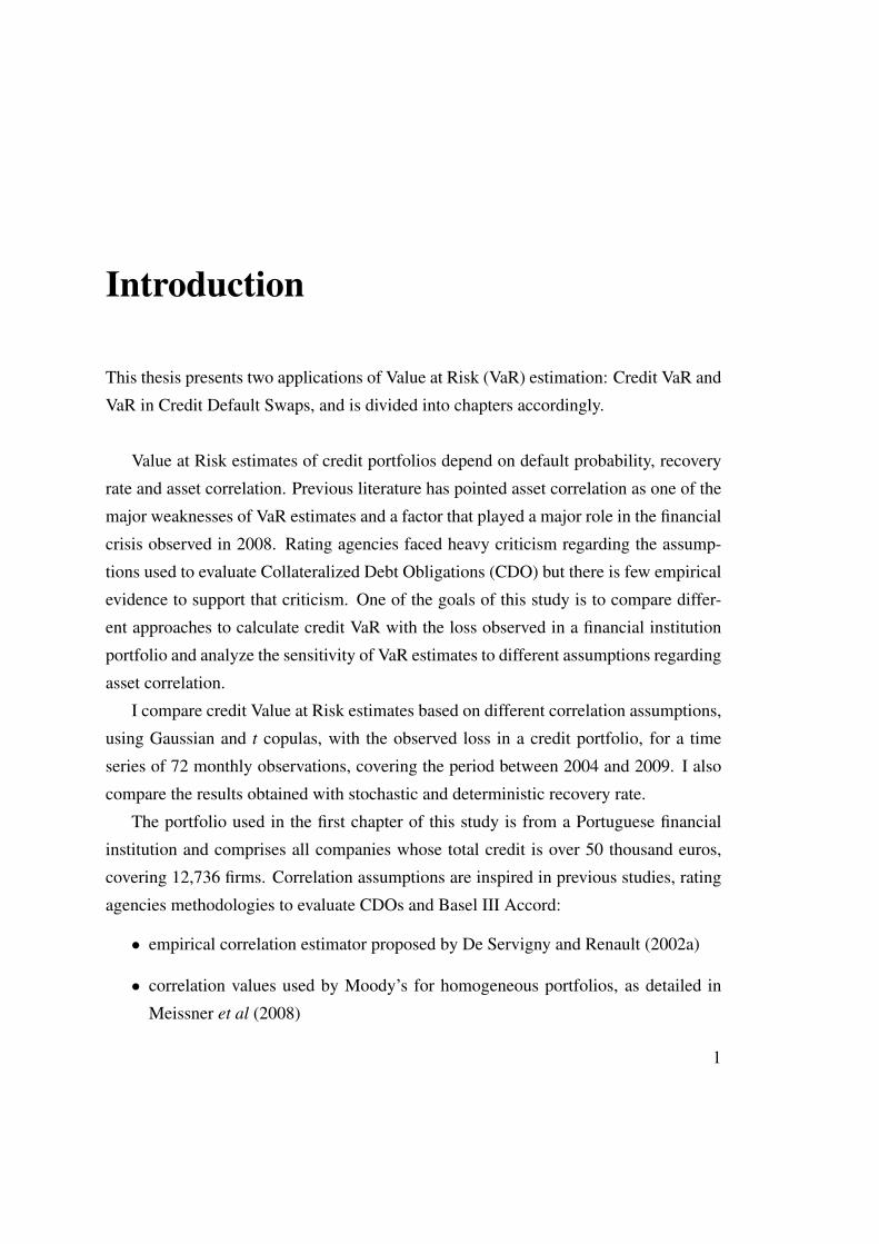
This thesis presents two applications of Value at Risk (VaR) estimation: Credit VaR and
VaR in Credit Default Swaps, and is divided into chapters accordingly.
Value at Risk estimates of credit portfolios depend on default probability, recovery
rate and asset correlation. Previous literature has pointed asset correlation as one of the
major weaknesses of VaR estimates and a factor that played a major role in the financial
crisis observed in 2008. Rating agencies faced heavy criticism regarding the assump-
tions used to evaluate Collateralized Debt Obligations (CDO) but there is few empirical
evidence to support that criticism. One of the goals of this study is to compare differ-
ent approaches to calculate credit VaR with the loss observed in a financial institution
portfolio and analyze the sensitivity of VaR estimates to different assumptions regarding
asset correlation.
I compare credit Value at Risk estimates based on different correlation assumptions,
using Gaussian and t copulas, with the observed loss in a credit portfolio, for a time
series of 72 monthly observations, covering the period between 2004 and 2009. I also
compare the results obtained with stochastic and deterministic recovery rate.
The portfolio used in the first chapter of this study is from a Portuguese financial
institution and comprises all companies whose total credit is over 50 thousand euros,
covering 12,736 firms. Correlation assumptions are inspired in previous studies, rating
agencies methodologies to evaluate CDOs and Basel III Accord:
• empirical correlation estimator proposed by De Servigny and Renault (2002a)
• correlation values used by Moody’s for homogeneous portfolios, as detailed in
Meissner et al (2008)
1
• correlation values used by Standard & Poors in their CDO Evaluator model, as
detailed in Meissner et al (2008)
• Standard & Poors’ old values (prior to 2005), as presented in Kiff (2004)
• approximation to Fitch’s asset correlation, following Fender and Kiff (2004)
• Basel III Accord’s maximum asset correlation
• Basel III Accord’s minimum asset correlation
Using Monte Carlo simulation technique and copula functions, I simulate portfolio
value distribution and compute credit VaR. Repeating this process for each monthly ob-
servation, I obtain the VaR time series, which I then compare with the time series of
observed loss in the portfolio using the tests proposed by Kupiec (1995) and Christof-
fersen (1998), the Loss Function method proposed by Lopez (1998) and the Average
Quantile Loss Function proposed by Koenker and Bassett (1978). Regarding VaR back-
testing, I also employ a measure of VaR over-conservativeness.
I find that credit VaR estimates differ substantially, depending on the assumptions
regarding asset correlation and dependence structure. This finding reinforces the cru-
cial role that the assumption regarding correlation plays in credit VaR estimation. I also
provide empirical evidence that some of the assumptions made by major rating agencies
to evaluate CDOs are inadequate in stress situations like the financial crisis observed in
2008. I find that the more accurate VaR model for the portfolio used in this study is
based on asset correlation given by the empirical estimator of De Servigny and Renault
(2002a) and assuming t copula with 8 degrees of freedom. All of the conclusions of
this study are invariant to the assumption of deterministic instead of stochastic recovery
rate, which suggests that it is possible to significantly reduce computation time with low
impact on the final results.
Credit Default Swaps (CDS) were at the forefront of the recent financial crisis of
2007-2009. CDS are essentially insurance contracts that protect against default of an
underlying company (the reference entity or name) and thus the CDS price is a measure
of the credit risk of the underlying obligor. During the crisis, CDS prices increased by
2
factors of 10, signalling high risk of default and potentially very large losses for the
financial institutions working as insurance companies in the CDS market. Therefore,
many observers have blamed CDS as one of the lead causes of the crisis. However, a
more careful analysis, as done in Stulz (2009), suggests that CDS did not trigger the
crisis and that in fact they allowed some institutions to limit their losses and, for this
reason, CDS are certain to remain a crucial financial instrument, even though under
tighter regulation and more control.
The financial crisis has raised more concern about risk prediction, which now has a
more important role in banking and finance. Banks rely on Value at Risk (VaR) mea-
sures to control their risk exposure. There are several competing approaches to estimate
VaR, including Historical Simulation using past data, parametric models describing the
full distribution of interest, Extreme Value Theory and Quantile Regression to model a
specific quantile rather than the whole distribution. The goal of this study is to estimate
VaR in CDS using Quantile Regression, covering the period of the recent financial crisis,
and perform a thorough evaluation of VaR estimates and compare them with alternative
VaR estimation methods through backtesting methodologies such as the tests proposed
by Kupiec (1995) and Christoffersen (1998), the Average Quantile Loss Function pro-
posed by Koenker and Bassett (1978), the Conditional Tail Expectation proposed by
Artzner et al (1999) and the Dynamic Quantile test presented by Engle and Manganelli
(2004). Quantile regression is potentially useful for estimating VaR in new products
with a short history. Furthermore, by incorporating current market expectations em-
bedded in the market prices of the explanatory variables, Quantile Regression has the
potential to outperform other methods when market conditions become very different
from the past.
I find that Quantile Regression provides better results in the estimation of VaR in
CDS than Historical Simulation, Filtered Historical Simulation, Extreme Value Theory
and all GARCH-based models tested in this study, especially for CDS names with long
history when the forecast horizon of VaR estimates is 30 days and for CDS names with
short history when the forecast horizon of VaR estimates is 1 day. I also find that the
financial ratios proposed by Campbell et al (2008) to determine the risk of bankruptcy
and failure contribute to explain the determinants of the price of CDS. Recent studies
3

have shown that Filtered Historical Simulation and Extreme Valued Theory are the most
accurate VaR models. However, the empirical evidence provided in this study does not
support the extension of this finding to VaR estimation in CDS.
4
Chapter 1
Credit VaR
5
1.1 Literature Review
Recent literature has shown that one of the main weaknesses in Credit Value at Risk
estimates is the assumption about correlation.The subprime crisis has shown that this
weakness is real.
Niethammer and Overbeck (2008) analyze the effect of estimation errors on risk
figures, causing model risk. They point out that estimating correlation is of major im-
portance for banks and find empirical evidence that the obtained values of correlation
strongly depend on the method used in the estimation. Crouhy et al (2000) show that
credit VaR is quite sensitive to estimates of correlations. In this paper, I provide em-
pirical evidence of the sensitivity of credit VaR estimates to the assumptions regarding
correlation by calculating credit VaR for a real portfolio considering several correlation
assumptions.
According to Duffie (2008), even specialists in CDOs are ill equipped to measure
the risk of tranches that are sensitive to default correlation and this is the weakest link in
credit risk transfer markets, which could suffer a dramatic loss of liquidity if a surprise
cluster of defaults suddenly emerges. Moreover, he argues that correlation parameters
used in rating methodologies tend to be based on rudimentary assumptions. Picone
(2002) states that the main question in evaluating CDOs has become how to measure
the level of diversification in the portfolio, i.e., default correlations. Fender and Kiff
(2004) illustrate that incorrect assumptions about default correlation can cause the rat-
ing agencies to significantly under or overestimate the risk in a credit portfolio. A com-
parative analysis of Fitch, Moody’s and Standard and Poor’s CDO rating approaches
is provided by Meissner et al (2008). They conclude that at the end of 2007 the main
rating agencies were all applying the Merton Structural Model and deriving asset val-
ues with Gaussian copula model. The differences between methodologies existed in the
way the rating agencies derived the core input parameters, namely default probability,
recovery rate and asset correlation. Asset correlation was pointed out as the most crit-
ical input parameter, due to its significant impact on default distribution. In this paper
I estimate credit VaR considering the asset correlation assumptions used by the major
rating agencies to evaluate CDOs, for the period between 2004 and 2009, and com-
pare these estimates with the observed loss in a real portfolio using VaR backtesting
6
methodologies. Due to the fact that the time period considered in this study covers the
subprime crisis and the portfolio considered in the analysis could have been securitized,
this study provides interesting insights about the accuracy of rating agencies method-
ologies to evaluate CDOs and also provides empirical evidence to the recent criticism
faced by rating agencies.
Several authors criticize the use of the Gaussian copula as market practice to esti-
mate VaR and evaluate CDOs. Previous research has shown that the assumption of the
same correlation parameters under different copulas may lead to hazardous understate-
ment of risk. According to Dorey et al (2005), the use of Gaussian copula seems to be
justified for modeling convenience rather than for theoretical reasons and this methodol-
ogy significantly underestimates the frequency of multiple extreme defaults. Frey et al
(2001) indicate that asset correlations are not enough to describe dependence between
defaults because they do not fully specify the copula of the latent variables. As a con-
sequence, the assumption of a Gaussian copula may not adequately model the potential
extreme risk in the portfolio. They also indicate that models allowing for tail depen-
dence, such as the multivariate t copula, give evidence that more worrying scenarios are
possible. Mashal and Zeevi (2002) perform a sensitivity analysis that strongly suggests
that the Gaussian dependence structure should be rejected in all data sets, when tested
against the alternative t dependence structure. According to Crouhy et al (2000), it is
not legitimate to assume normality of the portfolio changes for credit returns which are
by nature highly skewed and fat-tailed.The percentile levels of the distribution can not
be estimated from the variance only, the calculation of credit VaR requires drawing the
full distribution of changes in the portfolio. On the other hand, Hamerle and Rosch
(2005) show that misspecification of the distribution and the dependence structure of
asset returns does not necessarily produce misleading forecasts of the loss distribution.
In order to evaluate the impact of the choice of copula on the final results, I estimate
VaR with Gaussian and t copula, considering the correlation assumptions used by major
rating agencies and the Basel III Accord, and compare these estimates with the observed
loss.
7

1.2 Data
The data set used in this study is from one of the 10 largest Portuguese financial institu-
tions. The sample used in this study comprises all companies whose total credit is over
50 thousand euros, covering 12,736 firms in the period between January 2004 and De-
cember 2009. Table 1.1 presents the distribution of observations per year and industry.
Table 1.1: Distribution of observations per year and industryDistribution of the observations used in the empirical analysis, per year and industry, for the periodfrom January 2004 to December 2009.
YearIndustry 2004 2005 2006 2007 2008 2009
Banking and Finance 33 34 36 44 61 73
Broadcasting/Media/Cable 15 16 18 23 25 27
Building, Materials and Real Estate 2,712 2,866 3,051 3,222 3,269 3,161
Business Services 184 200 242 271 343 429
Materials and Utilities 40 48 50 60 69 91
Computers and Electronics 20 22 25 39 40 57
Consumer Products 604 611 704 863 1.052 1.262
Food, Beverage and Tobacco 63 72 88 122 146 170
Gaming, Leisure and Entertainment 171 180 201 213 228 275
Health Care and Pharmaceutical 73 90 100 114 132 148
Industrial/Manufacturing 204 219 257 330 394 489
Lodging and Restaurants 183 211 235 293 376 459
Retail 171 193 213 247 301 380
Supermarkets and Drugstores 482 516 584 658 756 979
Textiles and Furniture 93 100 109 124 156 202
Transportation 32 32 45 69 109 147
Others 47 42 49 49 71 81
Portfolio distribution per type of loan and guarantee are presented in tables 1.2 and
1.3. More than half of the total credit is guaranteed by real estate collateral, partly due
to the high weight of construction loans, namely 43.10%. Approximately 9% of the
portfolio has financial collateral and only 13.37% has no guarantee.
8
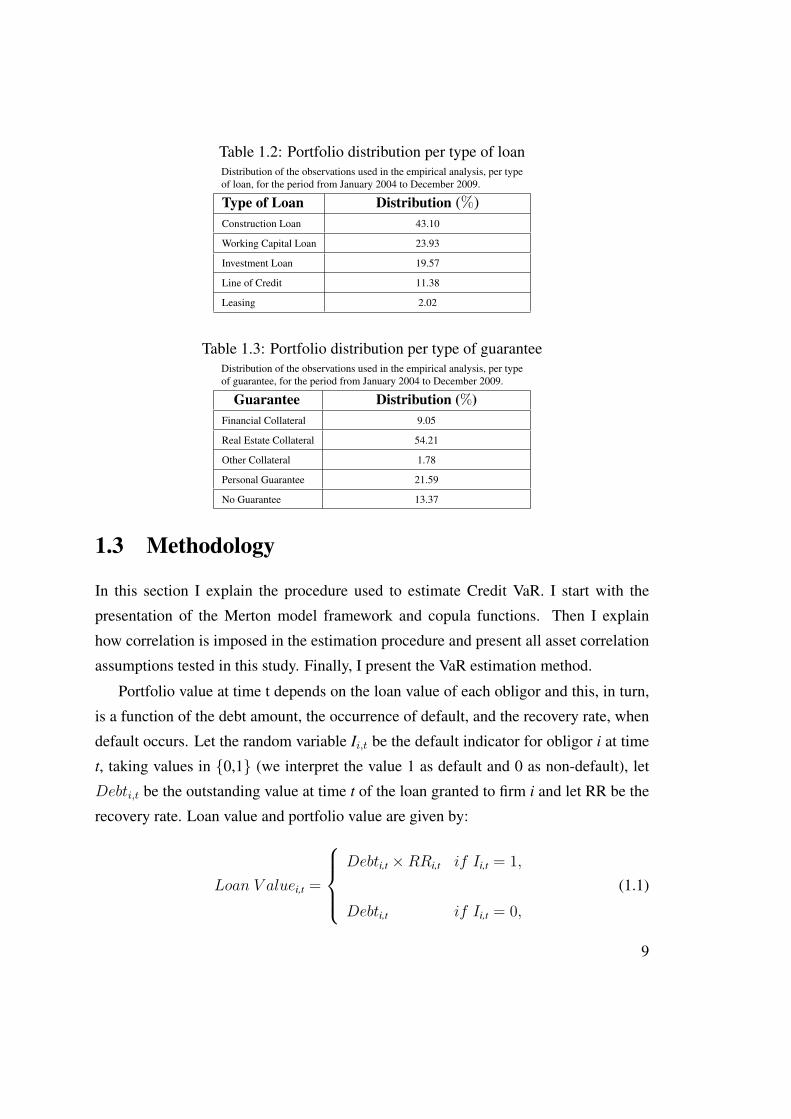
Table 1.2: Portfolio distribution per type of loanDistribution of the observations used in the empirical analysis, per typeof loan, for the period from January 2004 to December 2009.
Type of Loan Distribution (%)Construction Loan 43.10
Working Capital Loan 23.93
Investment Loan 19.57
Line of Credit 11.38
Leasing 2.02
Table 1.3: Portfolio distribution per type of guaranteeDistribution of the observations used in the empirical analysis, per typeof guarantee, for the period from January 2004 to December 2009.
Guarantee Distribution (%)Financial Collateral 9.05
Real Estate Collateral 54.21
Other Collateral 1.78
Personal Guarantee 21.59
No Guarantee 13.37
1.3 Methodology
In this section I explain the procedure used to estimate Credit VaR. I start with the
presentation of the Merton model framework and copula functions. Then I explain
how correlation is imposed in the estimation procedure and present all asset correlation
assumptions tested in this study. Finally, I present the VaR estimation method.
Portfolio value at time t depends on the loan value of each obligor and this, in turn,
is a function of the debt amount, the occurrence of default, and the recovery rate, when
default occurs. Let the random variable Ii,t be the default indicator for obligor i at time
t, taking values in 0,1 (we interpret the value 1 as default and 0 as non-default), let
Debti,t be the outstanding value at time t of the loan granted to firm i and let RR be the
recovery rate. Loan value and portfolio value are given by:
Loan V aluei,t =
Debti,t ×RRi,t if Ii,t = 1,
Debti,t if Ii,t = 0,
(1.1)
9
Portfolio V aluet =N∑i=1
Loan V aluei,t (1.2)
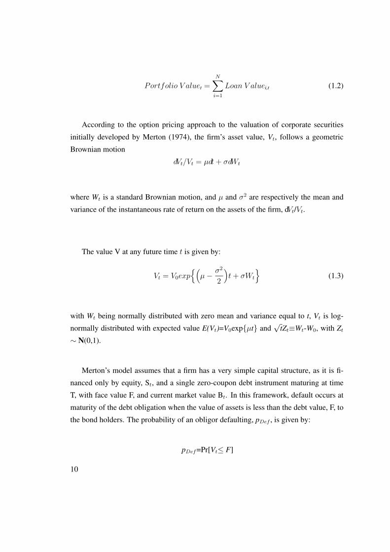
According to the option pricing approach to the valuation of corporate securities
initially developed by Merton (1974), the firm’s asset value, Vt, follows a geometric
Brownian motion
dVt/Vt = µdt+ σdWt
where Wt is a standard Brownian motion, and µ and σ2 are respectively the mean and
variance of the instantaneous rate of return on the assets of the firm, dVt/Vt.
The value V at any future time t is given by:
Vt = V0exp(µ− σ2
2
)t+ σWt
(1.3)
with Wt being normally distributed with zero mean and variance equal to t, Vt is log-
normally distributed with expected value E(Vt)=V0expµt and√
tZt≡Wt-W0, with Zt∼ N(0,1).
Merton’s model assumes that a firm has a very simple capital structure, as it is fi-
nanced only by equity, St, and a single zero-coupon debt instrument maturing at time
T, with face value F, and current market value Bt. In this framework, default occurs at
maturity of the debt obligation when the value of assets is less than the debt value, F, to
the bond holders. The probability of an obligor defaulting, pDef , is given by:
pDef=Pr[Vt≤ F]
10
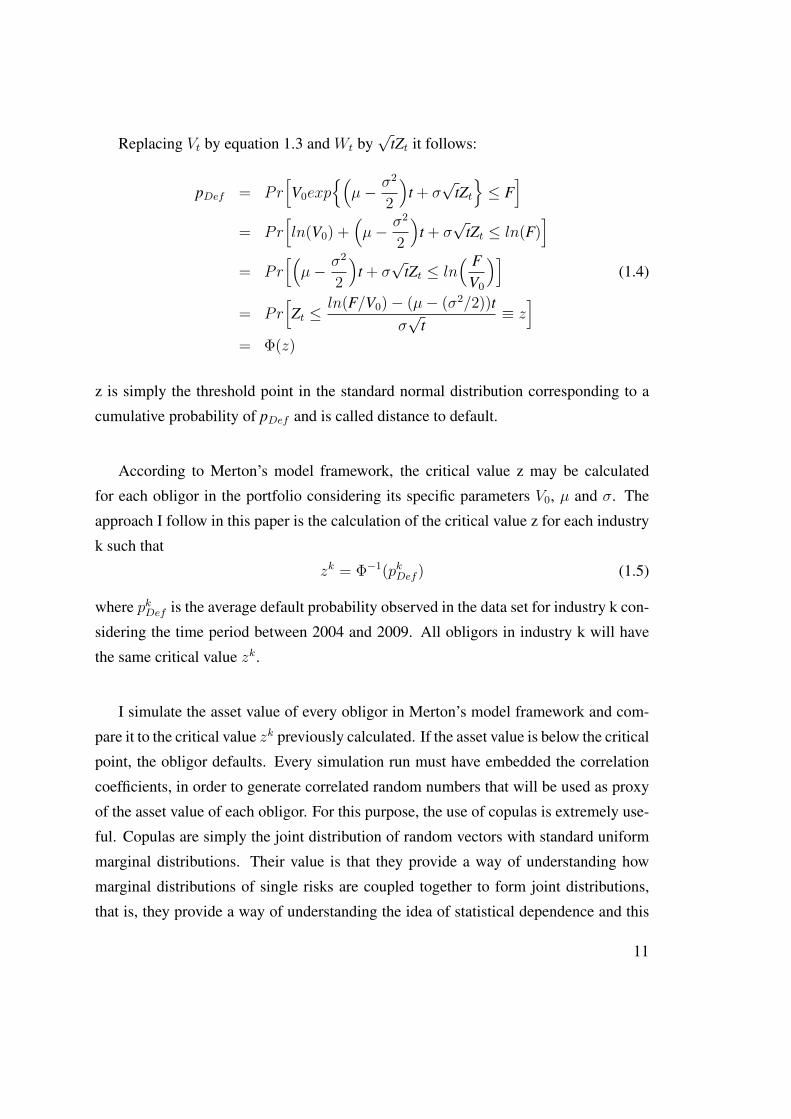
Replacing Vt by equation 1.3 and Wt by√
tZt it follows:
pDef = Pr[V0exp
(µ− σ2
2
)t + σ
√tZt≤ F
]= Pr
[ln(V0) +
(µ− σ2
2
)t + σ
√tZt ≤ ln(F)
]= Pr
[(µ− σ2
2
)t + σ
√tZt ≤ ln
( FV0
)](1.4)
= Pr[Zt ≤
ln(F/V0)− (µ− (σ2/2))tσ√
t≡ z]
= Φ(z)
z is simply the threshold point in the standard normal distribution corresponding to a
cumulative probability of pDef and is called distance to default.
According to Merton’s model framework, the critical value z may be calculated
for each obligor in the portfolio considering its specific parameters V0, µ and σ. The
approach I follow in this paper is the calculation of the critical value z for each industry
k such that
zk = Φ−1(pkDef ) (1.5)
where pkDef is the average default probability observed in the data set for industry k con-
sidering the time period between 2004 and 2009. All obligors in industry k will have
the same critical value zk.
I simulate the asset value of every obligor in Merton’s model framework and com-
pare it to the critical value zk previously calculated. If the asset value is below the critical
point, the obligor defaults. Every simulation run must have embedded the correlation
coefficients, in order to generate correlated random numbers that will be used as proxy
of the asset value of each obligor. For this purpose, the use of copulas is extremely use-
ful. Copulas are simply the joint distribution of random vectors with standard uniform
marginal distributions. Their value is that they provide a way of understanding how
marginal distributions of single risks are coupled together to form joint distributions,
that is, they provide a way of understanding the idea of statistical dependence and this
11
is the essence of Sklar’s theorem.
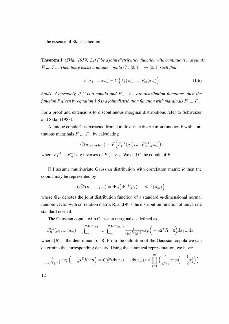
Theorem 1 (Sklar, 1959) Let F be a joint distribution function with continuous marginals
F1,...,Fm. Then there exists a unique copula C : [0, 1]m→ [0, 1] such that
F (x1, ..., xm) = C(F1(x1), ..., Fm(xm)
)(1.6)
holds. Conversely, if C is a copula and F1,...,Fm are distribution functions, then the
function F given by equation 1.6 is a joint distribution function with marginals F1,...,Fm.
For a proof and extensions to discontinuous marginal distributions refer to Schweizer
and Sklar (1983).
A unique copula C is extracted from a multivariate distribution function F with con-
tinuous marginals F1,...,Fm by calculating
C(µ1, ..., µm) = F(F−1
1 (µ1), ..., F−1m (µm)
),
where F−11 ,...,F−1
m are inverses of F1,...,Fm. We call C the copula of F.
If I assume multivariate Gaussian distribution with correlation matrix R then the
copula may be represented by
CGaR (µ1, ..., µm) = ΦR
(Φ−1(µ1), ...,Φ−1(µm)
),
where ΦR denotes the joint distribution function of a standard m-dimensional normal
random vector with correlation matrix R, and Φ is the distribution function of univariate
standard normal.
The Gaussian copula with Gaussian marginals is defined as
CGaR (µ1, ..., µm) =
∫Φ−1(µ1)
−∞...
∫Φ−1(µm)
−∞1
(2π)m2 |R|
12exp(− 1
2xTR−1x
)dx1...dxm
where |R| is the determinant of R. From the definition of the Gaussian copula we can
determine the corresponding density. Using the canonical representation, we have:
1
(2π)m2 |R|
12exp(− 1
2xTR−1x
)= CGa
R (Φ(x1), ...,Φ(xm))×m∏j=1
( 1√2πexp(− 1
2x2j
))12
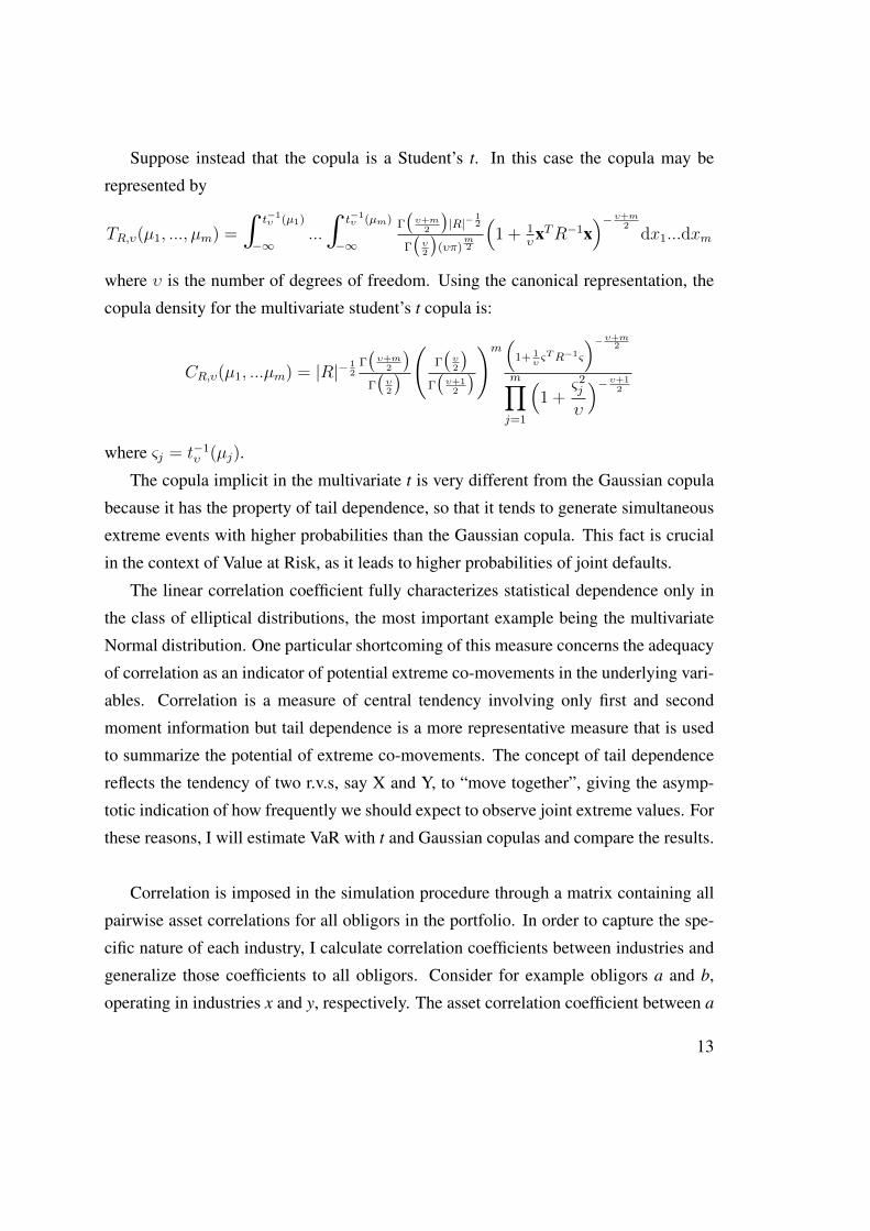
Suppose instead that the copula is a Student’s t. In this case the copula may be
represented by
TR,υ(µ1, ..., µm) =
∫t−1υ (µ1)
−∞...
∫t−1υ (µm)
−∞
Γ(υ+m
2
)|R|−
12
Γ(υ2
)(υπ)
m2
(1 + 1
υxTR−1x
)−υ+m2
dx1...dxm
where υ is the number of degrees of freedom. Using the canonical representation, the
copula density for the multivariate student’s t copula is:
CR,υ(µ1, ...µm) = |R|− 12
Γ(υ+m
2
)Γ(υ2
) ( Γ(υ2
)Γ(υ+12
))m(
1+ 1υςTR−1ς
)−υ+m2
m∏j=1
(1 +
ς2j
υ
)−υ+12
where ςj = t−1υ (µj).
The copula implicit in the multivariate t is very different from the Gaussian copula
because it has the property of tail dependence, so that it tends to generate simultaneous
extreme events with higher probabilities than the Gaussian copula. This fact is crucial
in the context of Value at Risk, as it leads to higher probabilities of joint defaults.
The linear correlation coefficient fully characterizes statistical dependence only in
the class of elliptical distributions, the most important example being the multivariate
Normal distribution. One particular shortcoming of this measure concerns the adequacy
of correlation as an indicator of potential extreme co-movements in the underlying vari-
ables. Correlation is a measure of central tendency involving only first and second
moment information but tail dependence is a more representative measure that is used
to summarize the potential of extreme co-movements. The concept of tail dependence
reflects the tendency of two r.v.s, say X and Y, to “move together”, giving the asymp-
totic indication of how frequently we should expect to observe joint extreme values. For
these reasons, I will estimate VaR with t and Gaussian copulas and compare the results.
Correlation is imposed in the simulation procedure through a matrix containing all
pairwise asset correlations for all obligors in the portfolio. In order to capture the spe-
cific nature of each industry, I calculate correlation coefficients between industries and
generalize those coefficients to all obligors. Consider for example obligors a and b,
operating in industries x and y, respectively. The asset correlation coefficient between a
13
and b, ρAab, will be given by the asset correlation between industries x and y.
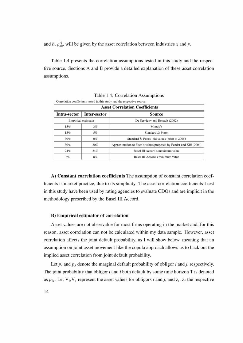
Table 1.4 presents the correlation assumptions tested in this study and the respec-
tive source. Sections A and B provide a detailed explanation of these asset correlation
assumptions.
Table 1.4: Correlation AssumptionsCorrelation coefficients tested in this study and the respective source.
Asset Correlation CoefficientsIntra-sector Inter-sector Source
Empirical estimator De Servigny and Renault (2002)
15% 3% Moody’s
15% 5% Standard & Poors
30% 0% Standard & Poors’ old values (prior to 2005)
30% 20% Approximation to Fitch’s values proposed by Fender and Kiff (2004)
24% 24% Basel III Accord’s maximum value
8% 8% Basel III Accord’s minimum value
A) Constant correlation coefficients The assumption of constant correlation coef-
ficients is market practice, due to its simplicity. The asset correlation coefficients I test
in this study have been used by rating agencies to evaluate CDOs and are implicit in the
methodology prescribed by the Basel III Accord.
B) Empirical estimator of correlation
Asset values are not observable for most firms operating in the market and, for this
reason, asset correlation can not be calculated within my data sample. However, asset
correlation affects the joint default probability, as I will show below, meaning that an
assumption on joint asset movement like the copula approach allows us to back out the
implied asset correlation from joint default probability.
Let pi and pj denote the marginal default probability of obligor i and j, respectively.
The joint probability that obligor i and j both default by some time horizon T is denoted
as pij . Let Vi,Vj represent the asset values for obligors i and j, and zi, zj the respective
14
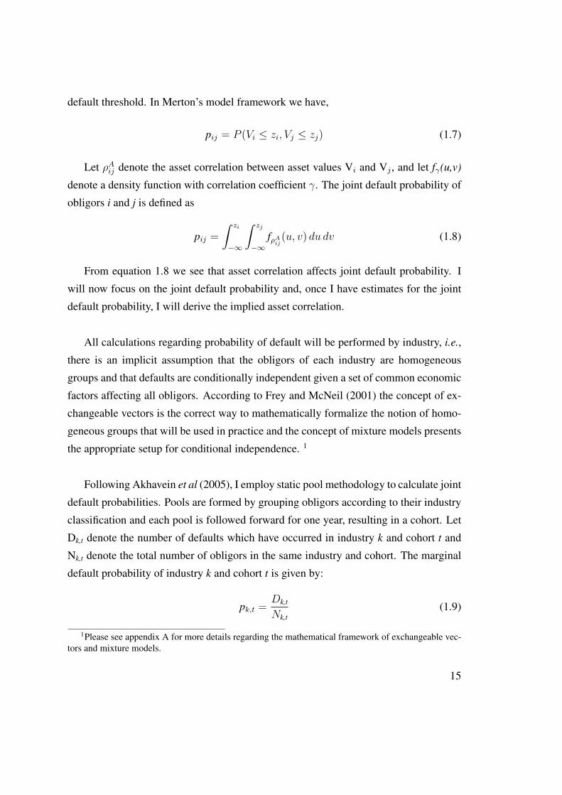
default threshold. In Merton’s model framework we have,
pij = P (Vi ≤ zi, Vj ≤ zj) (1.7)
Let ρAij denote the asset correlation between asset values Vi and Vj , and let fγ(u,v)
denote a density function with correlation coefficient γ. The joint default probability of
obligors i and j is defined as
pij =
∫ zi
−∞
∫ zj
−∞fρAij(u, v) du dv (1.8)
From equation 1.8 we see that asset correlation affects joint default probability. I
will now focus on the joint default probability and, once I have estimates for the joint
default probability, I will derive the implied asset correlation.
All calculations regarding probability of default will be performed by industry, i.e.,
there is an implicit assumption that the obligors of each industry are homogeneous
groups and that defaults are conditionally independent given a set of common economic
factors affecting all obligors. According to Frey and McNeil (2001) the concept of ex-
changeable vectors is the correct way to mathematically formalize the notion of homo-
geneous groups that will be used in practice and the concept of mixture models presents
the appropriate setup for conditional independence. 1
Following Akhavein et al (2005), I employ static pool methodology to calculate joint
default probabilities. Pools are formed by grouping obligors according to their industry
classification and each pool is followed forward for one year, resulting in a cohort. Let
Dk,t denote the number of defaults which have occurred in industry k and cohort t and
Nk,t denote the total number of obligors in the same industry and cohort. The marginal
default probability of industry k and cohort t is given by:
pk,t =Dk,t
Nk,t(1.9)
1Please see appendix A for more details regarding the mathematical framework of exchangeable vec-tors and mixture models.
15
The sample from 2004 to 2009 enables me to calculate 6 default probabilities for each
industry.
Once yearly default probabilities are calculated, I aggregate them to an average prob-
ability over the observation period, assuming that each year is an independent data set.
I weight each year by its relative size, that is, by the number of firms present in the
sample each year. The marginal default probability of industry k aggregated across all
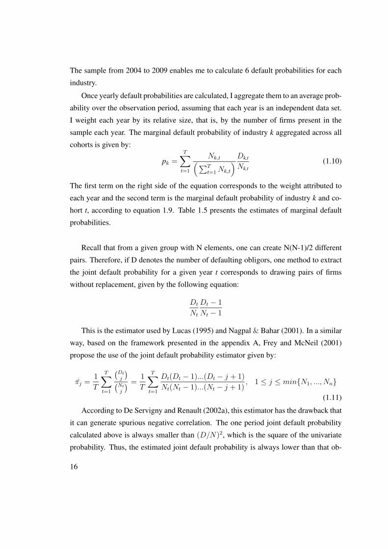
cohorts is given by:
pk =T∑t=1
Nk,t(∑Tt=1 Nk,t
)Dk,t
Nk,t(1.10)
The first term on the right side of the equation corresponds to the weight attributed to
each year and the second term is the marginal default probability of industry k and co-
hort t, according to equation 1.9. Table 1.5 presents the estimates of marginal default
probabilities.
Recall that from a given group with N elements, one can create N(N-1)/2 different
pairs. Therefore, if D denotes the number of defaulting obligors, one method to extract
the joint default probability for a given year t corresponds to drawing pairs of firms
without replacement, given by the following equation:
Dt
Nt
Dt − 1
Nt − 1
This is the estimator used by Lucas (1995) and Nagpal & Bahar (2001). In a similar
way, based on the framework presented in the appendix A, Frey and McNeil (2001)
propose the use of the joint default probability estimator given by:
πj =1
T
T∑t=1
(Dtj
)(Ntj
) =1
T
T∑t=1
Dt(Dt − 1)...(Dt − j + 1)
Nt(Nt − 1)...(Nt − j + 1), 1 ≤ j ≤ minN1, ..., Nn
(1.11)
According to De Servigny and Renault (2002a), this estimator has the drawback that
it can generate spurious negative correlation. The one period joint default probability
calculated above is always smaller than (D/N)2, which is the square of the univariate
probability. Thus, the estimated joint default probability is always lower than that ob-
16
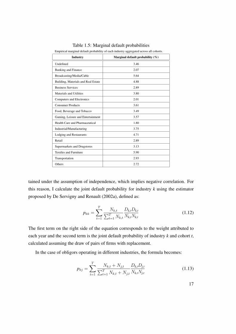
Table 1.5: Marginal default probabilitiesEmpirical marginal default probability of each industry aggregated across all cohorts.
Industry Marginal default probability (%)
Undefined 3.46
Banking and Finance 2.07
Broadcasting/Media/Cable 5.64
Building, Materials and Real Estate 4.88
Business Services 2.89
Materials and Utilities 3.80
Computers and Electronics 2.01
Consumer Products 3.61
Food, Beverage and Tobacco 3.49
Gaming, Leisure and Entertainment 3.57
Health Care and Pharmaceutical 1.80
Industrial/Manufacturing 3.75
Lodging and Restaurants 4.71
Retail 2.89
Supermarkets and Drugstores 3.13
Textiles and Furniture 5.90
Transportation 2.93
Others 2.72
tained under the assumption of independence, which implies negative correlation. For
this reason, I calculate the joint default probability for industry k using the estimator
proposed by De Servigny and Renault (2002a), defined as:
pkk =T∑t=1
Nk,t∑Tt=1Nk,t
Dk,tDk,t
Nk,tNk,t(1.12)
The first term on the right side of the equation corresponds to the weight attributed to
each year and the second term is the joint default probability of industry k and cohort t,
calculated assuming the draw of pairs of firms with replacement.
In the case of obligors operating in different industries, the formula becomes:
pkj =T∑t=1
Nk,t +Nj,t∑Tt=1Nk,t +Nj,t
Dk,tDj,t
Nk,tNj,t(1.13)
17
Despite the fact that both estimators would yield very similar results in very large sam-
ples, in samples of the size of a typical credit portfolio the difference may be substantial.
For details regarding the performance of these estimators, see De Servigny and Renault
(2003). Table 1.6 presents the obtained estimates of joint default probabilities.
Once I have the joint default probabilities, I calculate the asset correlations implicit
in equation 1.8 using a numerical method. For this purpose, I assume multivariate Gaus-
sian distribution with Gaussian marginals. Table 1.7 presents the asset correlations ob-
tained imposing the restriction |pkj-pkj| ≤ 5× 10⁻⁶. The average intra sector asset cor-
relation is 12.99% and the average inter sector asset correlation is 0.14%, corresponding
to an average default correlation of 2.68% and 0.05%, respectively.
18
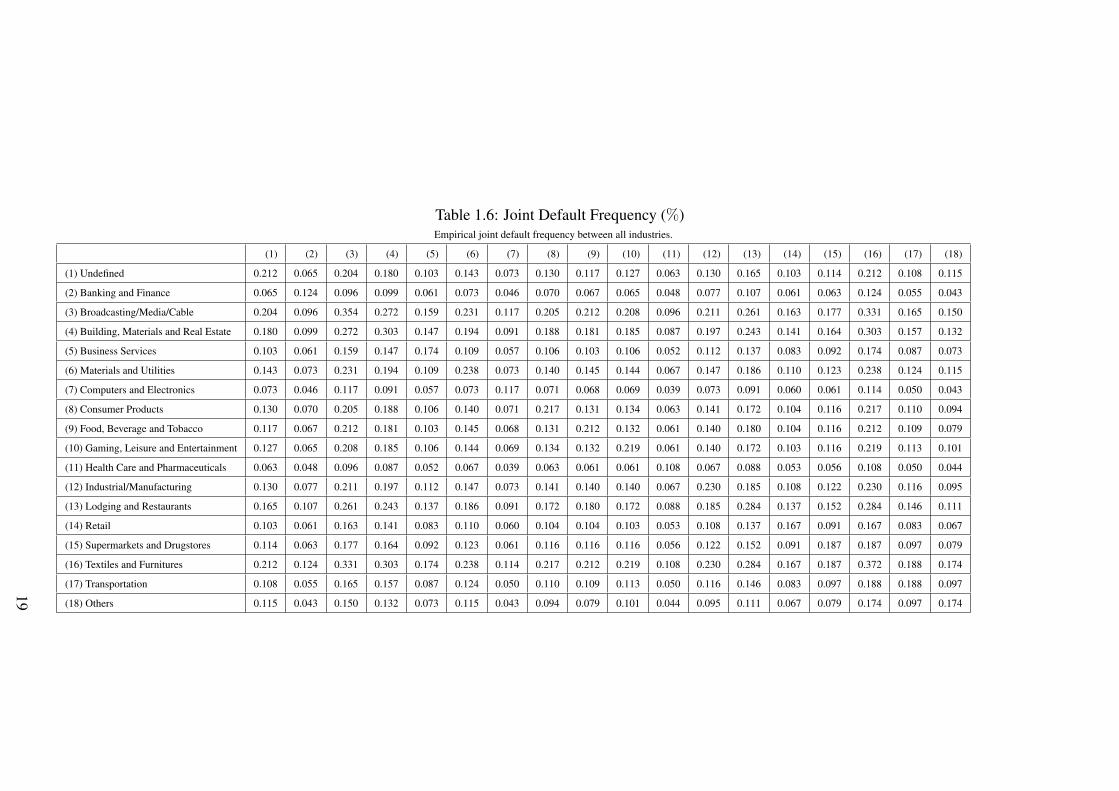
Table 1.6: Joint Default Frequency (%)Empirical joint default frequency between all industries.
(1) (2) (3) (4) (5) (6) (7) (8) (9) (10) (11) (12) (13) (14) (15) (16) (17) (18)
(1) Undefined 0.212 0.065 0.204 0.180 0.103 0.143 0.073 0.130 0.117 0.127 0.063 0.130 0.165 0.103 0.114 0.212 0.108 0.115
(2) Banking and Finance 0.065 0.124 0.096 0.099 0.061 0.073 0.046 0.070 0.067 0.065 0.048 0.077 0.107 0.061 0.063 0.124 0.055 0.043
(3) Broadcasting/Media/Cable 0.204 0.096 0.354 0.272 0.159 0.231 0.117 0.205 0.212 0.208 0.096 0.211 0.261 0.163 0.177 0.331 0.165 0.150
(4) Building, Materials and Real Estate 0.180 0.099 0.272 0.303 0.147 0.194 0.091 0.188 0.181 0.185 0.087 0.197 0.243 0.141 0.164 0.303 0.157 0.132
(5) Business Services 0.103 0.061 0.159 0.147 0.174 0.109 0.057 0.106 0.103 0.106 0.052 0.112 0.137 0.083 0.092 0.174 0.087 0.073
(6) Materials and Utilities 0.143 0.073 0.231 0.194 0.109 0.238 0.073 0.140 0.145 0.144 0.067 0.147 0.186 0.110 0.123 0.238 0.124 0.115
(7) Computers and Electronics 0.073 0.046 0.117 0.091 0.057 0.073 0.117 0.071 0.068 0.069 0.039 0.073 0.091 0.060 0.061 0.114 0.050 0.043
(8) Consumer Products 0.130 0.070 0.205 0.188 0.106 0.140 0.071 0.217 0.131 0.134 0.063 0.141 0.172 0.104 0.116 0.217 0.110 0.094
(9) Food, Beverage and Tobacco 0.117 0.067 0.212 0.181 0.103 0.145 0.068 0.131 0.212 0.132 0.061 0.140 0.180 0.104 0.116 0.212 0.109 0.079
(10) Gaming, Leisure and Entertainment 0.127 0.065 0.208 0.185 0.106 0.144 0.069 0.134 0.132 0.219 0.061 0.140 0.172 0.103 0.116 0.219 0.113 0.101
(11) Health Care and Pharmaceuticals 0.063 0.048 0.096 0.087 0.052 0.067 0.039 0.063 0.061 0.061 0.108 0.067 0.088 0.053 0.056 0.108 0.050 0.044
(12) Industrial/Manufacturing 0.130 0.077 0.211 0.197 0.112 0.147 0.073 0.141 0.140 0.140 0.067 0.230 0.185 0.108 0.122 0.230 0.116 0.095
(13) Lodging and Restaurants 0.165 0.107 0.261 0.243 0.137 0.186 0.091 0.172 0.180 0.172 0.088 0.185 0.284 0.137 0.152 0.284 0.146 0.111
(14) Retail 0.103 0.061 0.163 0.141 0.083 0.110 0.060 0.104 0.104 0.103 0.053 0.108 0.137 0.167 0.091 0.167 0.083 0.067
(15) Supermarkets and Drugstores 0.114 0.063 0.177 0.164 0.092 0.123 0.061 0.116 0.116 0.116 0.056 0.122 0.152 0.091 0.187 0.187 0.097 0.079
(16) Textiles and Furnitures 0.212 0.124 0.331 0.303 0.174 0.238 0.114 0.217 0.212 0.219 0.108 0.230 0.284 0.167 0.187 0.372 0.188 0.174
(17) Transportation 0.108 0.055 0.165 0.157 0.087 0.124 0.050 0.110 0.109 0.113 0.050 0.116 0.146 0.083 0.097 0.188 0.188 0.097
(18) Others 0.115 0.043 0.150 0.132 0.073 0.115 0.043 0.094 0.079 0.101 0.044 0.095 0.111 0.067 0.079 0.174 0.097 0.174
19
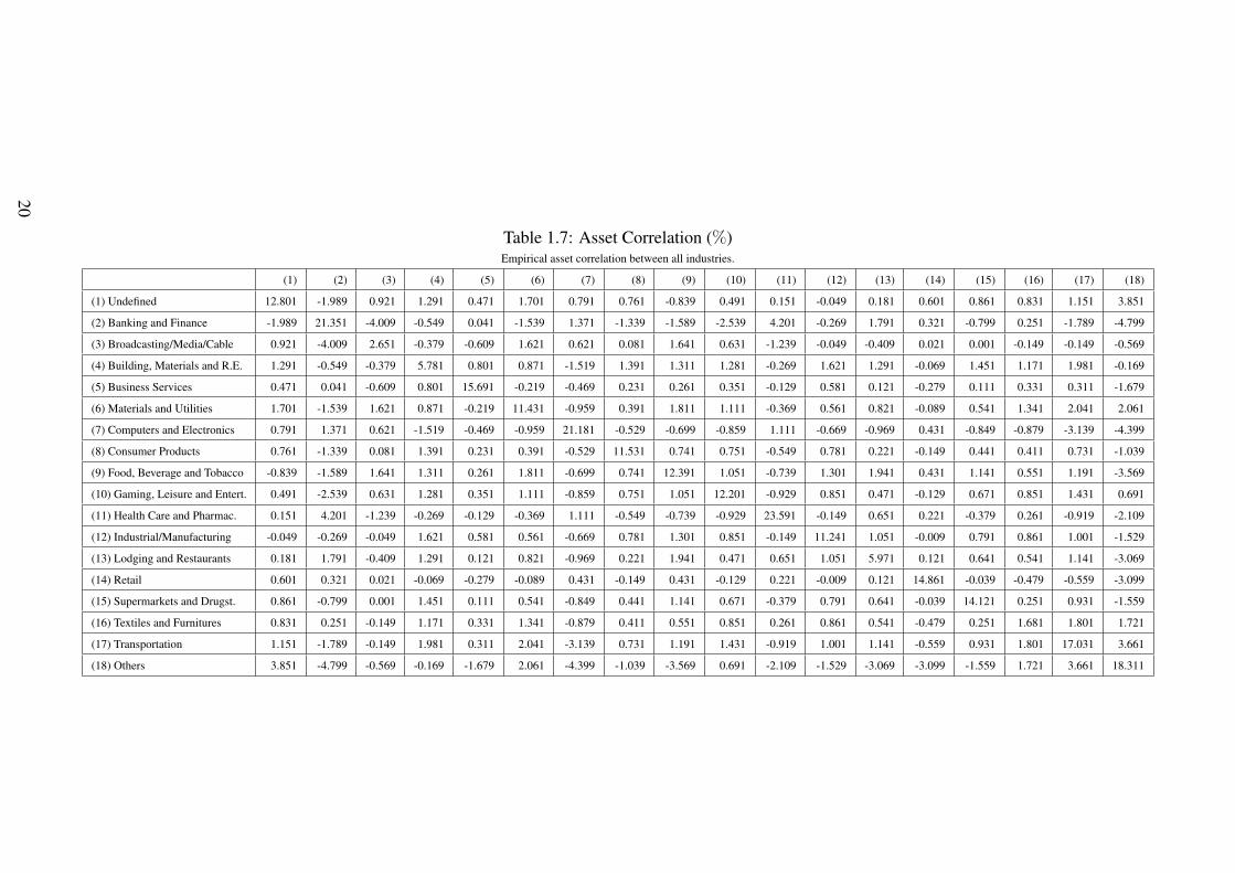
Table 1.7: Asset Correlation (%)Empirical asset correlation between all industries.
(1) (2) (3) (4) (5) (6) (7) (8) (9) (10) (11) (12) (13) (14) (15) (16) (17) (18)
(1) Undefined 12.801 -1.989 0.921 1.291 0.471 1.701 0.791 0.761 -0.839 0.491 0.151 -0.049 0.181 0.601 0.861 0.831 1.151 3.851
(2) Banking and Finance -1.989 21.351 -4.009 -0.549 0.041 -1.539 1.371 -1.339 -1.589 -2.539 4.201 -0.269 1.791 0.321 -0.799 0.251 -1.789 -4.799
(3) Broadcasting/Media/Cable 0.921 -4.009 2.651 -0.379 -0.609 1.621 0.621 0.081 1.641 0.631 -1.239 -0.049 -0.409 0.021 0.001 -0.149 -0.149 -0.569
(4) Building, Materials and R.E. 1.291 -0.549 -0.379 5.781 0.801 0.871 -1.519 1.391 1.311 1.281 -0.269 1.621 1.291 -0.069 1.451 1.171 1.981 -0.169
(5) Business Services 0.471 0.041 -0.609 0.801 15.691 -0.219 -0.469 0.231 0.261 0.351 -0.129 0.581 0.121 -0.279 0.111 0.331 0.311 -1.679
(6) Materials and Utilities 1.701 -1.539 1.621 0.871 -0.219 11.431 -0.959 0.391 1.811 1.111 -0.369 0.561 0.821 -0.089 0.541 1.341 2.041 2.061
(7) Computers and Electronics 0.791 1.371 0.621 -1.519 -0.469 -0.959 21.181 -0.529 -0.699 -0.859 1.111 -0.669 -0.969 0.431 -0.849 -0.879 -3.139 -4.399
(8) Consumer Products 0.761 -1.339 0.081 1.391 0.231 0.391 -0.529 11.531 0.741 0.751 -0.549 0.781 0.221 -0.149 0.441 0.411 0.731 -1.039
(9) Food, Beverage and Tobacco -0.839 -1.589 1.641 1.311 0.261 1.811 -0.699 0.741 12.391 1.051 -0.739 1.301 1.941 0.431 1.141 0.551 1.191 -3.569
(10) Gaming, Leisure and Entert. 0.491 -2.539 0.631 1.281 0.351 1.111 -0.859 0.751 1.051 12.201 -0.929 0.851 0.471 -0.129 0.671 0.851 1.431 0.691
(11) Health Care and Pharmac. 0.151 4.201 -1.239 -0.269 -0.129 -0.369 1.111 -0.549 -0.739 -0.929 23.591 -0.149 0.651 0.221 -0.379 0.261 -0.919 -2.109
(12) Industrial/Manufacturing -0.049 -0.269 -0.049 1.621 0.581 0.561 -0.669 0.781 1.301 0.851 -0.149 11.241 1.051 -0.009 0.791 0.861 1.001 -1.529
(13) Lodging and Restaurants 0.181 1.791 -0.409 1.291 0.121 0.821 -0.969 0.221 1.941 0.471 0.651 1.051 5.971 0.121 0.641 0.541 1.141 -3.069
(14) Retail 0.601 0.321 0.021 -0.069 -0.279 -0.089 0.431 -0.149 0.431 -0.129 0.221 -0.009 0.121 14.861 -0.039 -0.479 -0.559 -3.099
(15) Supermarkets and Drugst. 0.861 -0.799 0.001 1.451 0.111 0.541 -0.849 0.441 1.141 0.671 -0.379 0.791 0.641 -0.039 14.121 0.251 0.931 -1.559
(16) Textiles and Furnitures 0.831 0.251 -0.149 1.171 0.331 1.341 -0.879 0.411 0.551 0.851 0.261 0.861 0.541 -0.479 0.251 1.681 1.801 1.721
(17) Transportation 1.151 -1.789 -0.149 1.981 0.311 2.041 -3.139 0.731 1.191 1.431 -0.919 1.001 1.141 -0.559 0.931 1.801 17.031 3.661
(18) Others 3.851 -4.799 -0.569 -0.169 -1.679 2.061 -4.399 -1.039 -3.569 0.691 -2.109 -1.529 -3.069 -3.099 -1.559 1.721 3.661 18.311
20
1.3.1 VaR Estimation2
Once I have the asset correlation matrix, I start generating correlated random numbers
that will be used as proxy of the asset value of each obligor. Let C=(C1,...,CN )′ be an
N-dimensional random vector with continuous marginal distributions representing the
asset value of each obligor and let z=(z1,...,zN )′ be a vector of deterministic cut-off levels
obtained within Merton’s model framework. The following relationship holds:
Ii = 1⇔ Ci ≤ zi (1.14)
I follow Monte Carlo simulation technique to draw the portfolio value distribution.
The first step is the generation of 10,000 scenarios for the asset value of each obligor i
in each time period t. In the case of Gaussian copula, a possible way of transforming a
vector of uncorrelated random variables (U) into a vector of correlated random variables
(C) is the multiplication of U by the Cholesky decomposition of the asset correlation
matrix Ωt. Considering a portfolio with N obligors, the Cholesky decomposition of Ωt
is the N×N symmetric positive definite lower triangular matrix At, such that Ωt=AtA′t.In the case of the t copula, the vector of correlated random variables is obtained from
the application of the appropriate copula function. By doing this, it is possible to have a
dependence structure with t-student distribution and marginals within the Merton model
framework.
After the simulation of the asset value for every obligor, I determine which obligors
default in each simulation s and time period t. When a default occurs, a recovery rate is
determined by using Beta distribution sampling. The probability density function of the
Beta distribution, for 0 ≤ x ≤ 1 and shape parameters α, β > 0, is given by:
Γ(α + β)
Γ(α)Γ(β)xα−1(1− x)β−1 (1.15)
2VaR estimation was performed with the software Matlab.
21
where Γ(z) is the gamma function. The expected value and variance of x are given by:
E[x] =α
α + βvar[x] =
αβ
(α + β)2(α + β + 1)(1.16)
The historical levels of recovery for this type of loans in the financial institution
considered in this study have an average value of 61% and a variance of 0.01668, which
are reflected in the following parameters of the Beta distribution: α equal to 8.09 and
β equal to 5.13. Loan value of obligor i in simulation s and time t is given by equation
1.1.
Portfolio value for simulation s in period t is represented by:
Portfolio V aluest =
N∑i=1
Loan V aluesi,t , s ∈ (1, ...10.000), t ∈ (1, ...72) (1.17)
After drawing portfolio value distribution for period t, the credit VaRt estimate for a
99% confidence level is calculated according to the following equation:
CV aR99%t = Mean portfolio valuet − portfolio value1%
t (1.18)
I repeat this process for each correlation assumption and each copula, in order to
estimate VaR with different methodologies and compare the results with the time series
of observed loss. For the t dependence structure, it is essentially the degrees of freedom
parameter that controls the extent of tail dependence and tendency to exhibit extreme co-
movements. Considering previous research performed by Dorey et al (2005), Cherubini
et al (2004) and Abid & Naifar (2008), I calculate VaR considering 2, 8 and 12 degrees
of freedom.
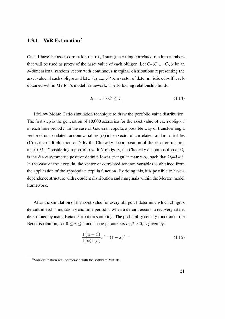
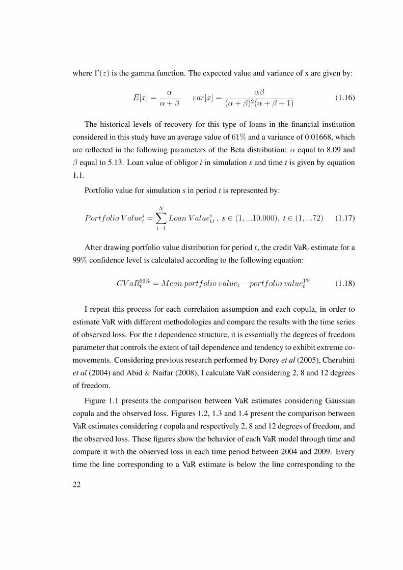
Figure 1.1 presents the comparison between VaR estimates considering Gaussian
copula and the observed loss. Figures 1.2, 1.3 and 1.4 present the comparison between
VaR estimates considering t copula and respectively 2, 8 and 12 degrees of freedom, and
the observed loss. These figures show the behavior of each VaR model through time and
compare it with the observed loss in each time period between 2004 and 2009. Every
time the line corresponding to a VaR estimate is below the line corresponding to the
22
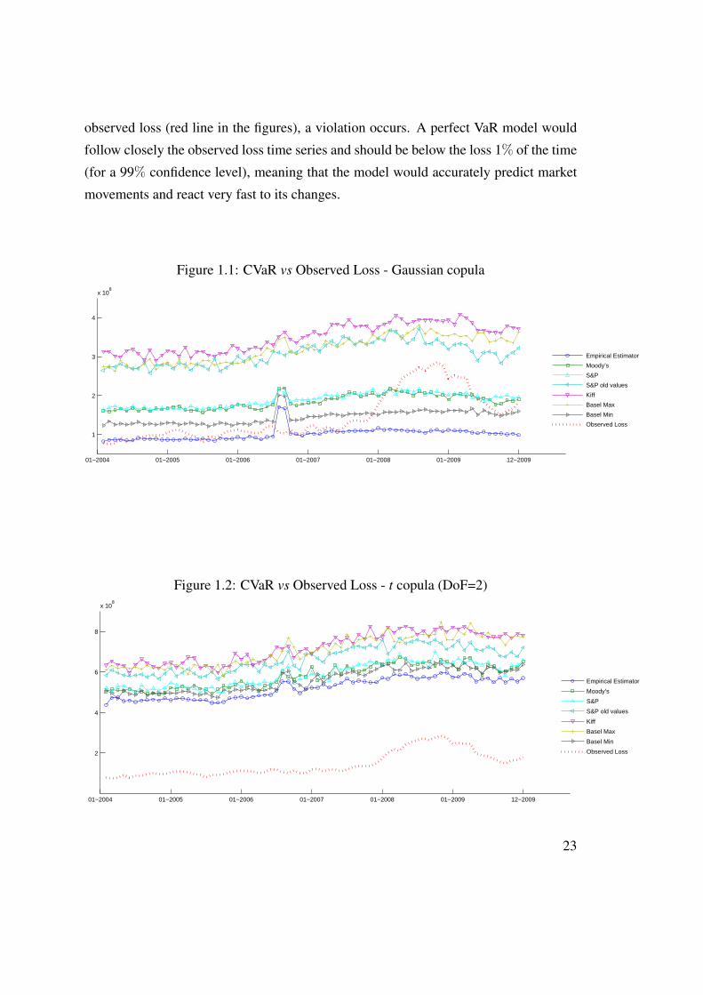
observed loss (red line in the figures), a violation occurs. A perfect VaR model would
follow closely the observed loss time series and should be below the loss 1% of the time
(for a 99% confidence level), meaning that the model would accurately predict market
movements and react very fast to its changes.
Figure 1.1: CVaR vs Observed Loss - Gaussian copula
01−2004 01−2005 01−2006 01−2007 01−2008 01−2009 12−2009
1
2
3
4
x 108
Empirical Estimator
Moody’s
S&P
S&P old values
Kiff
Basel Max
Basel Min
Observed Loss
Figure 1.2: CVaR vs Observed Loss - t copula (DoF=2)
01−2004 01−2005 01−2006 01−2007 01−2008 01−2009 12−2009
2
4
6
8
x 108
Empirical Estimator
Moody’s
S&P
S&P old values
Kiff
Basel Max
Basel Min
Observed Loss
23
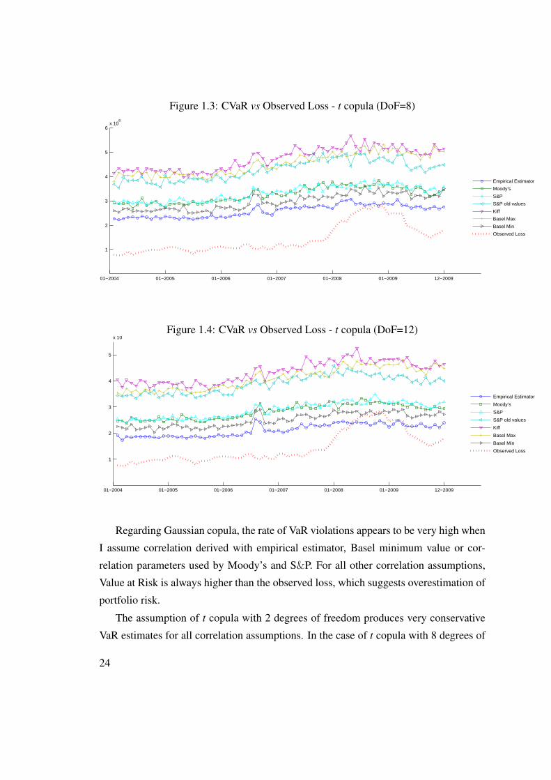
Figure 1.3: CVaR vs Observed Loss - t copula (DoF=8)
01−2004 01−2005 01−2006 01−2007 01−2008 01−2009 12−2009
1
2
3
4
5
6x 10
8
Empirical Estimator
Moody’s
S&P
S&P old values
Kiff
Basel Max
Basel Min
Observed Loss
Figure 1.4: CVaR vs Observed Loss - t copula (DoF=12)
01−2004 01−2005 01−2006 01−2007 01−2008 01−2009 12−2009
1
2
3
4
5
x 108
Empirical Estimator
Moody’s
S&P
S&P old values
Kiff
Basel Max
Basel Min
Observed Loss
Regarding Gaussian copula, the rate of VaR violations appears to be very high when
I assume correlation derived with empirical estimator, Basel minimum value or cor-
relation parameters used by Moody’s and S&P. For all other correlation assumptions,
Value at Risk is always higher than the observed loss, which suggests overestimation of
portfolio risk.
The assumption of t copula with 2 degrees of freedom produces very conservative
VaR estimates for all correlation assumptions. In the case of t copula with 8 degrees of
24
freedom, only the empirical estimator of correlation produces VaR violations. Increas-
ing the degrees of freedom from 8 to 12 apparently increases the number of VaR vio-
lations in the case of empirical estimator and Basel minimum value for asset correlation.
1.4 Backtesting VaR
The assumptions about correlation and dependence structure tested in this study pro-
duced very different VaR estimates. In order to compare the different VaR approaches
and identify the most accurate one, I perform backtesting procedures.
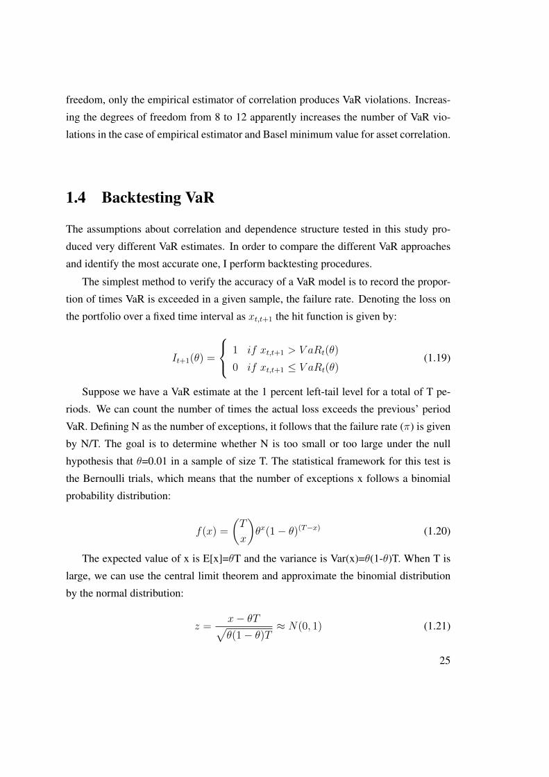
The simplest method to verify the accuracy of a VaR model is to record the propor-
tion of times VaR is exceeded in a given sample, the failure rate. Denoting the loss on
the portfolio over a fixed time interval as xt,t+1 the hit function is given by:
It+1(θ) =
1 if xt,t+1 > V aRt(θ)
0 if xt,t+1 ≤ V aRt(θ)(1.19)
Suppose we have a VaR estimate at the 1 percent left-tail level for a total of T pe-
riods. We can count the number of times the actual loss exceeds the previous’ period
VaR. Defining N as the number of exceptions, it follows that the failure rate (π) is given
by N/T. The goal is to determine whether N is too small or too large under the null
hypothesis that θ=0.01 in a sample of size T. The statistical framework for this test is
the Bernoulli trials, which means that the number of exceptions x follows a binomial
probability distribution:
f(x) =
(T
x
)θx(1− θ)(T−x) (1.20)
The expected value of x is E[x]=θT and the variance is Var(x)=θ(1-θ)T. When T is
large, we can use the central limit theorem and approximate the binomial distribution
by the normal distribution:
z =x− θT√θ(1− θ)T
≈ N(0, 1) (1.21)
25
Christoffersen (1998) points out that the problem of determining the accuracy of a
VaR model can be reduced to the problem of determining whether the hit sequence sat-
isfies two properties:
Unconditional coverage property: The probability of realizing a loss in excess of
the estimated VaR should be exactly θ. If losses in excess of the estimated VaR occur
more frequently than θ of the time, then this would suggest that the VaR model system-
atically understates the portfolio risk. The opposite finding would alternatively provide
evidence on an overly conservative VaR model.
Independence property: this property places a strong restriction on how VaR ex-
ceptions may occur. Intuitively, this condition requires that the previous history of VaR
violations must not convey any information about whether a VaR violation will occur
in the following period. In general, a clustering of VaR exceptions represents violation
of the independence property that provides evidence of a lack of responsiveness in the
VaR model, making successive runs of VaR exceptions more likely.
According to Campbell (2005), the unconditional coverage and independence prop-
erties of the hit sequence are distinct and must both be satisfied by an accurate VaR
model.
A) Kupiec Test (1995)
Kupiec (1995) proposes a test to check the unconditional coverage property, based
on the number of VaR violations. Kupiec’s test examines how many times a VaR is
violated over a given span of time. If the number of exceptions differs considerably
from θ × 100, then the accuracy of the VaR model is called into question. The null
hypothesis for Kupiec’s test is:
H0 : π = θ (1.22)
π is given by:
π =N
T(1.23)
26
The log-likelihood ratio for this test is given by:
LRuc = −2ln[(1− θ)T−NθN ] + 2ln[1− π]T−N πN (1.24)
which is asymptotically distributed chi-square with one degree of freedom under the
null hypothesis that θ is the true probability.
B) Christoffersen Test (1998)Christoffersen (1998) developed a test to check the independence property. The test
setup is as follows: each period we set a violation indicator to 0 if VaR is not exceeded
and to 1 otherwise. We then define Tij as the number of periods in which state j has
occurred in one period while it was i the previous period and πi as the probability of
observing an exception conditional on state i the previous period. The null hypothesis
is:
H0 : π0 = π1 = π (1.25)
The test statistic is given by:
LRind = −2ln[(1−π)(T00+T10)π(T01+T11)]+2ln[(1−π0)T00 π0T01(1−π1)T10 π1
T11 ] (1.26)
which is asymptotically distributed chi-square with one degree of freedom. π0 and π1
are given by:
π1 = T11T10+T11
π0 = T01T00+T01
Tables 1.8 and 1.9 present the results obtained for Kupiec and Christoffersen tests
for all correlation assumptions considering Gaussian and t copulas. The null hypothesis
of Kupiec test is rejected in the scenario of Gaussian copula considering asset correla-
tion based on the empirical estimator, Moody’s, S&P and Basel Accord minimum value.
The same result is obtained in the case of t copula with 12 degrees of freedom, consid-
ering asset correlation given by the empirical estimator. The null hypothesis of Kupiec
test is not rejected in the case of t copula with 8 degrees of freedom and correlation
based on the empirical estimator and also in the case of t copula with 12 degrees of
freedom and correlation based on Basel III Accord minimum value. In the remaining
27
correlation assumptions, Kupiec test is inconclusive due to the fact that no exceptions
were observed.
The null hypothesis of Christoffersen test is rejected in the case of Gaussian copula
with correlation based on Moody’s and S&P parameters and in the case of t copula
with 12 degrees of freedom with correlation based on the empirical estimator. The
null hypothesis of this test is not rejected only in the cases of Gaussian copula with
correlation based on the empirical estimator and t copula with 12 degrees of freedom
and correlation prescribed by Basel III Accord minimum value. In all the other cases
this test is inconclusive.
Since the unconditional coverage and independence properties of the hit sequence
must be both satisfied by an accurate VaR model, at this point I can conclude that some
of the models tested in this study are not accurate, namely the models based on Gaussian
copula with correlation given by the empirical estimator, Moody’s and S&P parameters
and Basel III Accord minimum value for correlation and also the model based on t cop-
ula with 12 degrees of freedom and correlation given by the empirical estimator. I will
exclude these VaR models from the remaining backtesting procedures.
At this point an interesting conclusion emerges: since the methodologies applied by
Moody’s and Standard and Poors to evaluate CDOs are based on the Gaussian copula
with the correlation parameters tested in this study and these methodologies produced
very high failure rates, leading to the rejection of the null hypothesis of the Kupiec test,
I conclude there is empirical evidence that the procedures used by major rating agencies
to evaluate CDOs are inadequate in stress situations like the financial crisis observed in
2008.
Some of the correlation assumptions tested in this study produced null failure rate
or null results for the statistics T10, T11, leading to inconclusive results of Kupiec and
Christoffersen tests. These null outcomes might be explained by over conservative VaR
models or by the small number of observations, but in either cases it is not possible to
draw a conclusion from the performed VaR backtests. The evaluation of the accuracy of
these VaR models requires us to find alternative methods.
28
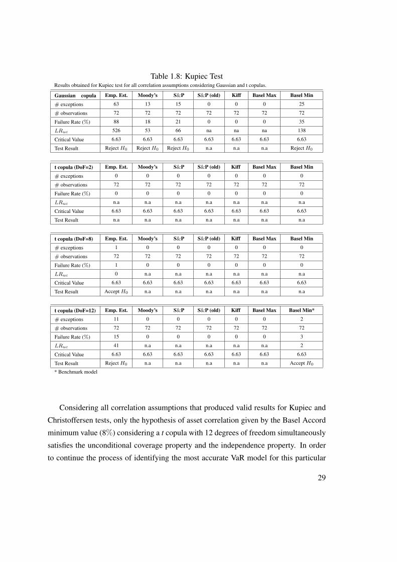
Table 1.8: Kupiec TestResults obtained for Kupiec test for all correlation assumptions considering Gaussian and t copulas.
Gaussian copula Emp. Est. Moody’s S&P S&P (old) Kiff Basel Max Basel Min
# exceptions 63 13 15 0 0 0 25
# observations 72 72 72 72 72 72 72
Failure Rate (%) 88 18 21 0 0 0 35
LRuc 526 53 66 na na na 138
Critical Value 6.63 6.63 6.63 6.63 6.63 6.63 6.63
Test Result Reject H0 Reject H0 Reject H0 n.a n.a n.a Reject H0
t copula (DoF=2) Emp. Est. Moody’s S&P S&P (old) Kiff Basel Max Basel Min
# exceptions 0 0 0 0 0 0 0
# observations 72 72 72 72 72 72 72
Failure Rate (%) 0 0 0 0 0 0 0
LRuc n.a n.a n.a n.a n.a n.a n.a
Critical Value 6.63 6.63 6.63 6.63 6.63 6.63 6.63
Test Result n.a n.a n.a n.a n.a n.a n.a
t copula (DoF=8) Emp. Est. Moody’s S&P S&P (old) Kiff Basel Max Basel Min
# exceptions 1 0 0 0 0 0 0
# observations 72 72 72 72 72 72 72
Failure Rate (%) 1 0 0 0 0 0 0
LRuc 0 n.a n.a n.a n.a n.a n.a
Critical Value 6.63 6.63 6.63 6.63 6.63 6.63 6.63
Test Result Accept H0 n.a n.a n.a n.a n.a n.a
t copula (DoF=12) Emp. Est. Moody’s S&P S&P (old) Kiff Basel Max Basel Min*
# exceptions 11 0 0 0 0 0 2
# observations 72 72 72 72 72 72 72
Failure Rate (%) 15 0 0 0 0 0 3
LRuc 41 n.a n.a n.a n.a n.a 2
Critical Value 6.63 6.63 6.63 6.63 6.63 6.63 6.63
Test Result Reject H0 n.a n.a n.a n.a n.a Accept H0
* Benchmark model
Considering all correlation assumptions that produced valid results for Kupiec and
Christoffersen tests, only the hypothesis of asset correlation given by the Basel Accord
minimum value (8%) considering a t copula with 12 degrees of freedom simultaneously
satisfies the unconditional coverage property and the independence property. In order
to continue the process of identifying the most accurate VaR model for this particular
29
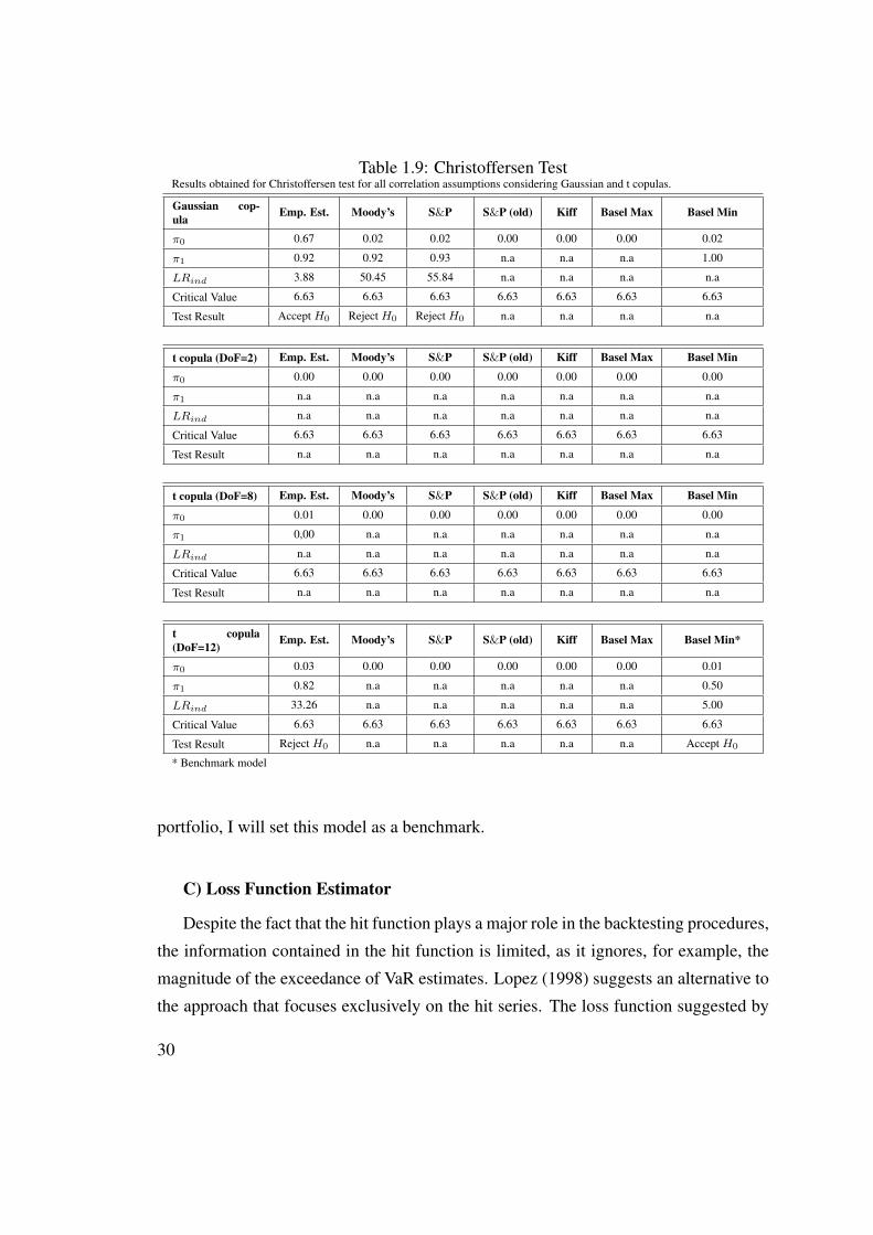
Table 1.9: Christoffersen TestResults obtained for Christoffersen test for all correlation assumptions considering Gaussian and t copulas.
Gaussian cop-ula
Emp. Est. Moody’s S&P S&P (old) Kiff Basel Max Basel Min
π0 0.67 0.02 0.02 0.00 0.00 0.00 0.02
π1 0.92 0.92 0.93 n.a n.a n.a 1.00
LRind 3.88 50.45 55.84 n.a n.a n.a n.a
Critical Value 6.63 6.63 6.63 6.63 6.63 6.63 6.63
Test Result Accept H0 Reject H0 Reject H0 n.a n.a n.a n.a
t copula (DoF=2) Emp. Est. Moody’s S&P S&P (old) Kiff Basel Max Basel Min
π0 0.00 0.00 0.00 0.00 0.00 0.00 0.00
π1 n.a n.a n.a n.a n.a n.a n.a
LRind n.a n.a n.a n.a n.a n.a n.a
Critical Value 6.63 6.63 6.63 6.63 6.63 6.63 6.63
Test Result n.a n.a n.a n.a n.a n.a n.a
t copula (DoF=8) Emp. Est. Moody’s S&P S&P (old) Kiff Basel Max Basel Min
π0 0.01 0.00 0.00 0.00 0.00 0.00 0.00
π1 0,00 n.a n.a n.a n.a n.a n.a
LRind n.a n.a n.a n.a n.a n.a n.a
Critical Value 6.63 6.63 6.63 6.63 6.63 6.63 6.63
Test Result n.a n.a n.a n.a n.a n.a n.a
t copula(DoF=12)
Emp. Est. Moody’s S&P S&P (old) Kiff Basel Max Basel Min*
π0 0.03 0.00 0.00 0.00 0.00 0.00 0.01
π1 0.82 n.a n.a n.a n.a n.a 0.50
LRind 33.26 n.a n.a n.a n.a n.a 5.00
Critical Value 6.63 6.63 6.63 6.63 6.63 6.63 6.63
Test Result Reject H0 n.a n.a n.a n.a n.a Accept H0
* Benchmark model
portfolio, I will set this model as a benchmark.
C) Loss Function Estimator
Despite the fact that the hit function plays a major role in the backtesting procedures,
the information contained in the hit function is limited, as it ignores, for example, the
magnitude of the exceedance of VaR estimates. Lopez (1998) suggests an alternative to
the approach that focuses exclusively on the hit series. The loss function suggested by
30
Lopez (1998) is:
L(V aRt(θ), xt,t+1) =
1 + (xt,t+1 − V aRt(θ))2 if xt,t+1 > V aRt(θ)
0 if xt,t+1 ≤ V aRt(θ)(1.27)
According to Campbell (2005), a backtest that uses the loss function defined by
Lopez (1998) would typically be based on the sample average loss,
L =1
T
T∑t=1
L(V aRt(θ), xt,t+1) (1.28)
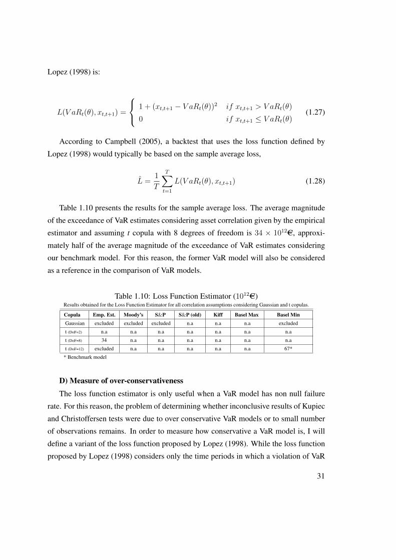
Table 1.10 presents the results for the sample average loss. The average magnitude
of the exceedance of VaR estimates considering asset correlation given by the empirical
estimator and assuming t copula with 8 degrees of freedom is 34 × 1012AC, approxi-
mately half of the average magnitude of the exceedance of VaR estimates considering
our benchmark model. For this reason, the former VaR model will also be considered
as a reference in the comparison of VaR models.
Table 1.10: Loss Function Estimator (1012AC)Results obtained for the Loss Function Estimator for all correlation assumptions considering Gaussian and t copulas.
Copula Emp. Est. Moody’s S&P S&P (old) Kiff Basel Max Basel MinGaussian excluded excluded excluded n.a n.a n.a excluded
t (DoF=2) n.a n.a n.a n.a n.a n.a n.a
t (DoF=8) 34 n.a n.a n.a n.a n.a n.a
t (DoF=12) excluded n.a n.a n.a n.a n.a 67*
* Benchmark model
D) Measure of over-conservativeness
The loss function estimator is only useful when a VaR model has non null failure
rate. For this reason, the problem of determining whether inconclusive results of Kupiec
and Christoffersen tests were due to over conservative VaR models or to small number
of observations remains. In order to measure how conservative a VaR model is, I will
define a variant of the loss function proposed by Lopez (1998). While the loss function
proposed by Lopez (1998) considers only the time periods in which a violation of VaR
31
occurs (in the remaining periods the function has value 0), this new measure considers
only the periods in which the loss is below the estimated VaR (assigning the value 0
when there is violation of the VaR estimate). Thus, we can calculate an average value
of over-conservativeness. The advantage of this measure of over-conservativeness is
that it provides additional information when the Kupiec and Christoffersen tests are
inconclusive.
L′(V aRt(θ), xt,t+1) =
1 + (V aRt(θ)− xt,t+1)2 if xt,t+1 < V aRt(θ)
0 if xt,t+1 ≥ V aRt(θ)(1.29)
Define N’ as the number of periods for which VaR estimates are higher than the actual
loss. The sample average is given by:
L′ =1
N ′
T∑t=1
L′(V aRt(θ), xt,t+1) (1.30)
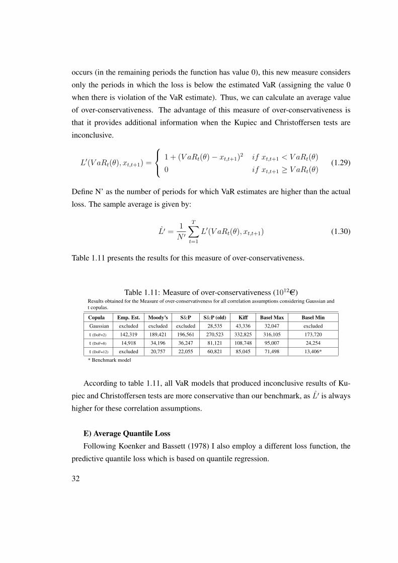
Table 1.11 presents the results for this measure of over-conservativeness.
Table 1.11: Measure of over-conservativeness (1012AC)Results obtained for the Measure of over-conservativeness for all correlation assumptions considering Gaussian andt copulas.
Copula Emp. Est. Moody’s S&P S&P (old) Kiff Basel Max Basel MinGaussian excluded excluded excluded 28,535 43,336 32,047 excluded
t (DoF=2) 142,319 189,421 196,561 270,523 332,825 316,105 173,720
t (DoF=8) 14,918 34,196 36,247 81,121 108,748 95,007 24,254
t (DoF=12) excluded 20,757 22,055 60,821 85,045 71,498 13,406*
* Benchmark model
According to table 1.11, all VaR models that produced inconclusive results of Ku-
piec and Christoffersen tests are more conservative than our benchmark, as L′ is always
higher for these correlation assumptions.
E) Average Quantile LossFollowing Koenker and Bassett (1978) I also employ a different loss function, the
predictive quantile loss which is based on quantile regression.
32
QL(V aRt(θ), xt,t+1) =
| xt,t+1 − V aRt(θ) | (θ) if xt,t+1 < V aRt(θ)
| xt,t+1 − V aRt(θ) | (1− θ) if xt,t+1 ≥ V aRt(θ)
(1.31)
The economic intuition behind the use of the QL function is that the capital forgone
from overpredicting the true VaR should also be taken into account. This function is
asymmetric in view of the fact that underestimation and overestimation have diverse
consequences, as underprediction of risk might lead to liquidity problems and insol-
vency, and overprediction implies higher capital charges which reflect the opportunity
cost of keeping a high reserve ratio. The best VaR method is the one that generates the
lowest average quantile loss (AQL), defined as:
AQL =1
T
T∑t=1
QL(V aRt(θ), xt,t+1) (1.32)
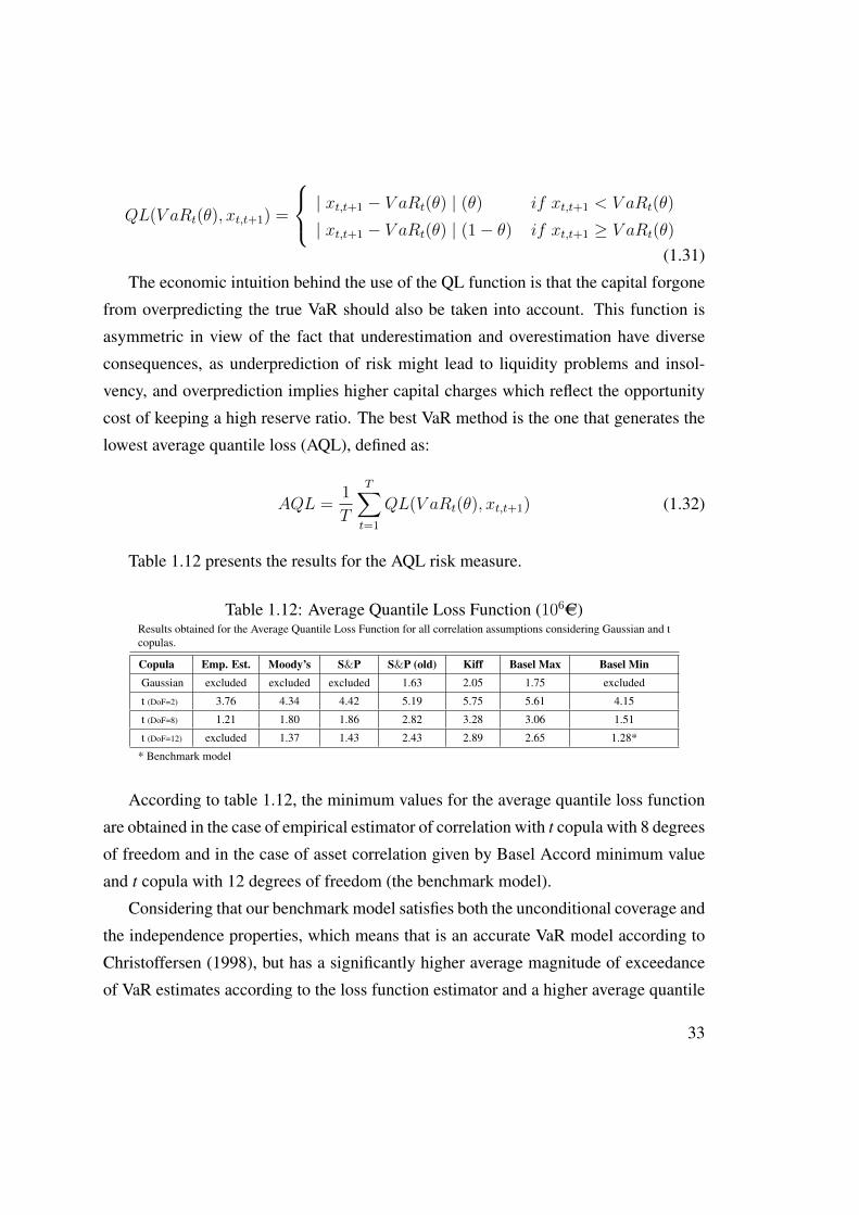
Table 1.12 presents the results for the AQL risk measure.
Table 1.12: Average Quantile Loss Function (106AC)Results obtained for the Average Quantile Loss Function for all correlation assumptions considering Gaussian and tcopulas.
Copula Emp. Est. Moody’s S&P S&P (old) Kiff Basel Max Basel MinGaussian excluded excluded excluded 1.63 2.05 1.75 excluded
t (DoF=2) 3.76 4.34 4.42 5.19 5.75 5.61 4.15
t (DoF=8) 1.21 1.80 1.86 2.82 3.28 3.06 1.51
t (DoF=12) excluded 1.37 1.43 2.43 2.89 2.65 1.28*
* Benchmark model
According to table 1.12, the minimum values for the average quantile loss function
are obtained in the case of empirical estimator of correlation with t copula with 8 degrees
of freedom and in the case of asset correlation given by Basel Accord minimum value
and t copula with 12 degrees of freedom (the benchmark model).
Considering that our benchmark model satisfies both the unconditional coverage and
the independence properties, which means that is an accurate VaR model according to
Christoffersen (1998), but has a significantly higher average magnitude of exceedance
of VaR estimates according to the loss function estimator and a higher average quantile
33
loss than the VaR model considering asset correlation given by the empirical estimator
and assuming t copula with 8 degrees of freedom, and that all the other VaR models are
either rejected in those tests or over conservative, I conclude that the most accurate VaR
model for this portfolio is based on asset correlation given by the empirical estimator
and assuming t copula with 8 degrees of freedom.
1.5 Deterministic versus Stochastic Recovery Rate
In the previous sections I presented VaR estimates assuming a recovery rate given by
Beta distribution sampling with parameters α equal to 8.09 and β equal to 5.13, both
estimated with historical information. In this section I present the results obtained as-
suming that the recovery rate is a constant proportion of the asset value and compare
them with the results produced with stochastic recovery rate.
Considering the parameters α and β estimated with historical information and the
result in equation 1.16, the expected value of the recovery rate is 61%. I will assume
that the recovery rate is constant and equal to this value in the simulation procedure.
I repeated the process of VaR estimation described in previous sections, for the same
portfolio, time periods and correlation assumptions, assuming a deterministic instead of
a stochastic recovery rate. Figures 1.5 to 1.8 present the comparison between all VaR
estimates with stochastic and deterministic recovery rates. The analysis of the graphs
suggests that VaR estimates considering deterministic recovery rates are very similar to
those obtained with stochastic recovery rates.
Tables 1.13 and 1.14 present the results of Kupiec and Christoffersen tests. Regard-
ing Kupiec test, the conclusions are exactly the same that we have previously obtained
with stochastic recovery rate. The results obtained in Christoffersen test considering
deterministic instead of stochastic recovery rate are different for the case of gaussian
copula considering the empirical estimator of correlation and Basel Accord minimum
value for asset correlation (the null hypothesis is now rejected for these correlation as-
sumptions). Despite these differences, the conclusions derived from both tests remain
unchanged and the benchmark model is also the model based on t copula with 12 de-
34
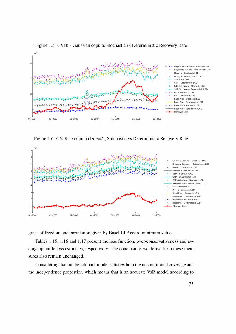
Figure 1.5: CVaR - Gaussian copula, Stochastic vs Deterministic Recovery Rate
01−2004 01−2005 01−2006 01−2007 01−2008 01−2009 12−2009
1
2
3
4
x 108
Empirical Estimator − Stochastic LGD
Empirical Estimator − Deterministic LGD
Moody’s − Stochastic LGD
Moody’s − Deterministic LGD
S&P − Stochastic LGD
S&P − Deterministic LGD
S&P Old values − Stochastic LGD
S&P Old values − Deterministic LGD
Kiff − Stochastic LGD
Kiff − Deterministic LGD
Basel Max − Stochastic LGD
Basel Max − Deterministic LGD
Basel Min − Stochastic LGD
Basel Min − Deterministic LGD
Observed Loss
Figure 1.6: CVaR - t copula (DoF=2), Stochastic vs Deterministic Recovery Rate
01−2004 01−2005 01−2006 01−2007 01−2008 01−2009 12−2009
1
2
3
4
5
6
7
8
9x 10
8
Empirical Estimator −Stochastic LGD
Empirical Estimator − Deterministic LGD
Moody’s − Stochastic LGD
Moody’s − Deterministic LGD
S&P − Stochastic LGD
S&P − Deterministic LGD
S&P Old values − Stochastic LGD
S&P Old values − Deterministic LGD
Kiff − Stochastic LGD
Kiff − Deterministic LGD
Basel Max − Stochastic LGD
Basel Max − Deterministic LGD
Basel Min − Stochastic LGD
Basel Min − Deterministic LGD
Observed Loss
grees of freedom and correlation given by Basel III Accord minimum value.
Tables 1.15, 1.16 and 1.17 present the loss function, over-conservativeness and av-
erage quantile loss estimates, respectively. The conclusions we derive from these mea-
sures also remain unchanged.
Considering that our benchmark model satisfies both the unconditional coverage and
the independence properties, which means that is an accurate VaR model according to
35
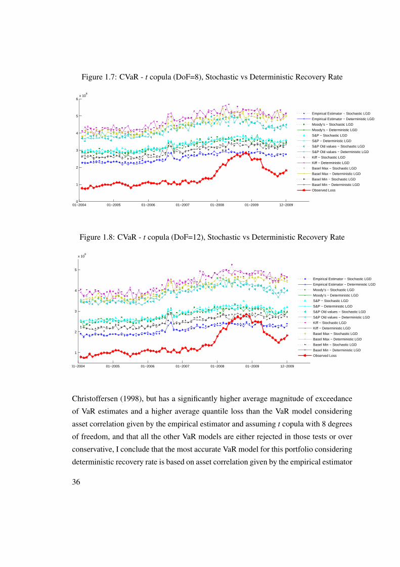
Figure 1.7: CVaR - t copula (DoF=8), Stochastic vs Deterministic Recovery Rate
01−2004 01−2005 01−2006 01−2007 01−2008 01−2009 12−20090
1
2
3
4
5
6x 10
8
Empirical Estimator − Stochastic LGD
Empirical Estimator − Deterministic LGD
Moody’s − Stochastic LGD
Moody’s − Deterministic LGD
S&P − Stochastic LGD
S&P − Deterministic LGD
S&P Old values − Stochastic LGD
S&P Old values − Deterministic LGD
Kiff − Stochastic LGD
Kiff − Deterministic LGD
Basel Max − Stochastic LGD
Basel Max − Deterministic LGD
Basel Min − Stochastic LGD
Basel Min − Deterministic LGD
Observed Loss
Figure 1.8: CVaR - t copula (DoF=12), Stochastic vs Deterministic Recovery Rate
01−2004 01−2005 01−2006 01−2007 01−2008 01−2009 12−2009
1
2
3
4
5
x 108
Empirical Estimator − Stochastic LGD
Empirical Estimator − Deterministic LGD
Moody’s − Stochastic LGD
Moody’s − Deterministic LGD
S&P − Stochastic LGD
S&P − Deterministic LGD
S&P Old values − Stochastic LGD
S&P Old values − Deterministic LGD
Kiff − Stochastic LGD
Kiff − Deterministic LGD
Basel Max − Stochastic LGD
Basel Max − Deterministic LGD
Basel Min − Stochastic LGD
Basel Min − Deterministic LGD
Observed Loss
Christoffersen (1998), but has a significantly higher average magnitude of exceedance
of VaR estimates and a higher average quantile loss than the VaR model considering
asset correlation given by the empirical estimator and assuming t copula with 8 degrees
of freedom, and that all the other VaR models are either rejected in those tests or over
conservative, I conclude that the most accurate VaR model for this portfolio considering
deterministic recovery rate is based on asset correlation given by the empirical estimator
36
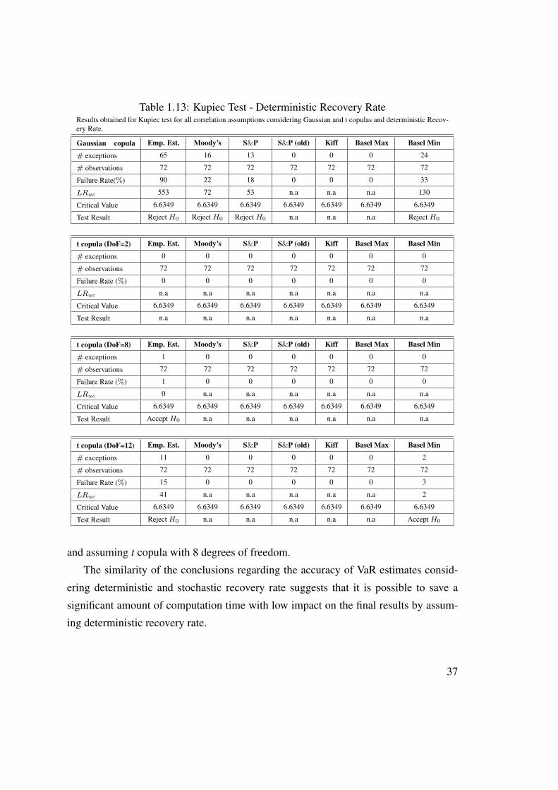
Table 1.13: Kupiec Test - Deterministic Recovery RateResults obtained for Kupiec test for all correlation assumptions considering Gaussian and t copulas and deterministic Recov-ery Rate.
Gaussian copula Emp. Est. Moody’s S&P S&P (old) Kiff Basel Max Basel Min
# exceptions 65 16 13 0 0 0 24
# observations 72 72 72 72 72 72 72
Failure Rate(%) 90 22 18 0 0 0 33
LRuc 553 72 53 n.a n.a n.a 130
Critical Value 6.6349 6.6349 6.6349 6.6349 6.6349 6.6349 6.6349
Test Result Reject H0 Reject H0 Reject H0 n.a n.a n.a Reject H0
t copula (DoF=2) Emp. Est. Moody’s S&P S&P (old) Kiff Basel Max Basel Min
# exceptions 0 0 0 0 0 0 0
# observations 72 72 72 72 72 72 72
Failure Rate (%) 0 0 0 0 0 0 0
LRuc n.a n.a n.a n.a n.a n.a n.a
Critical Value 6.6349 6.6349 6.6349 6.6349 6.6349 6.6349 6.6349
Test Result n.a n.a n.a n.a n.a n.a n.a
t copula (DoF=8) Emp. Est. Moody’s S&P S&P (old) Kiff Basel Max Basel Min
# exceptions 1 0 0 0 0 0 0
# observations 72 72 72 72 72 72 72
Failure Rate (%) 1 0 0 0 0 0 0
LRuc 0 n.a n.a n.a n.a n.a n.a
Critical Value 6.6349 6.6349 6.6349 6.6349 6.6349 6.6349 6.6349
Test Result Accept H0 n.a n.a n.a n.a n.a n.a
t copula (DoF=12) Emp. Est. Moody’s S&P S&P (old) Kiff Basel Max Basel Min
# exceptions 11 0 0 0 0 0 2
# observations 72 72 72 72 72 72 72
Failure Rate (%) 15 0 0 0 0 0 3
LRuc 41 n.a n.a n.a n.a n.a 2
Critical Value 6.6349 6.6349 6.6349 6.6349 6.6349 6.6349 6.6349
Test Result Reject H0 n.a n.a n.a n.a n.a Accept H0
and assuming t copula with 8 degrees of freedom.
The similarity of the conclusions regarding the accuracy of VaR estimates consid-
ering deterministic and stochastic recovery rate suggests that it is possible to save a
significant amount of computation time with low impact on the final results by assum-
ing deterministic recovery rate.
37
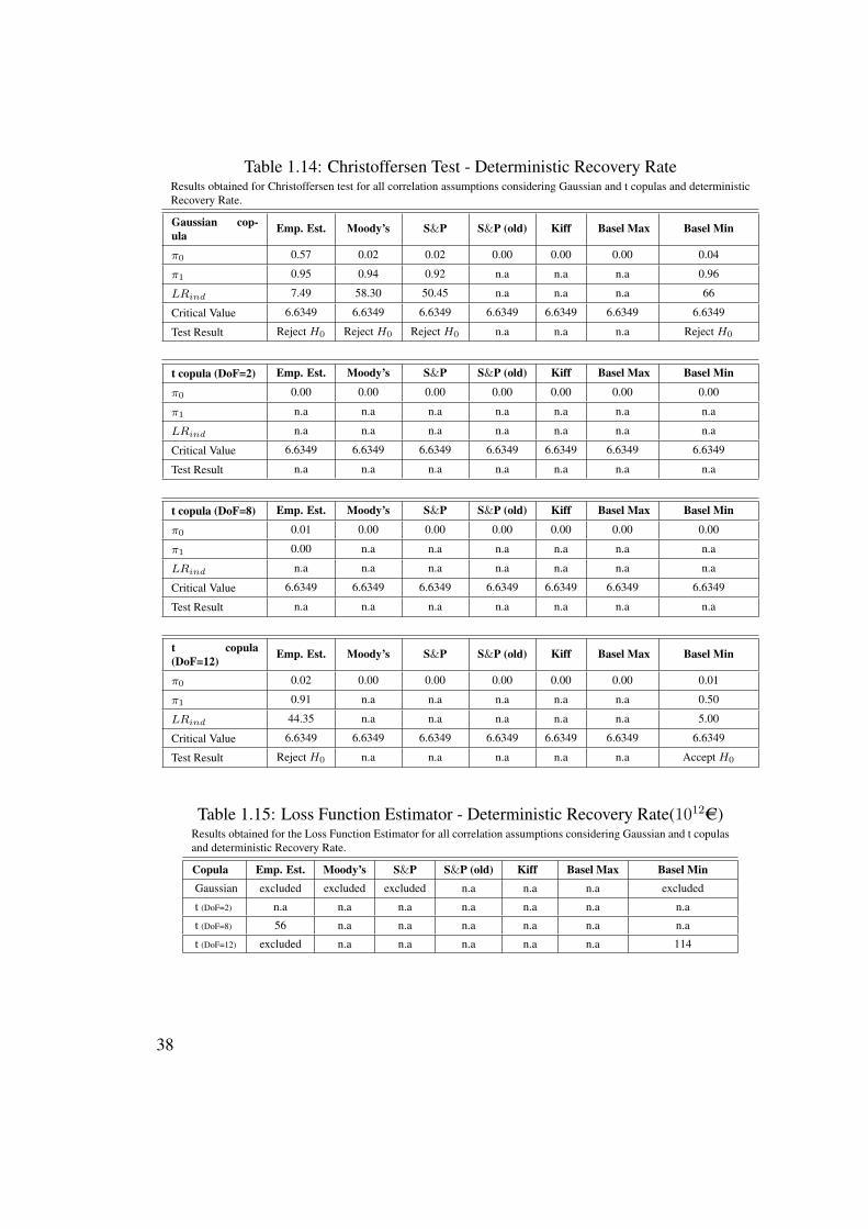
Table 1.14: Christoffersen Test - Deterministic Recovery RateResults obtained for Christoffersen test for all correlation assumptions considering Gaussian and t copulas and deterministicRecovery Rate.
Gaussian cop-ula
Emp. Est. Moody’s S&P S&P (old) Kiff Basel Max Basel Min
π0 0.57 0.02 0.02 0.00 0.00 0.00 0.04
π1 0.95 0.94 0.92 n.a n.a n.a 0.96
LRind 7.49 58.30 50.45 n.a n.a n.a 66
Critical Value 6.6349 6.6349 6.6349 6.6349 6.6349 6.6349 6.6349
Test Result Reject H0 Reject H0 Reject H0 n.a n.a n.a Reject H0
t copula (DoF=2) Emp. Est. Moody’s S&P S&P (old) Kiff Basel Max Basel Min
π0 0.00 0.00 0.00 0.00 0.00 0.00 0.00
π1 n.a n.a n.a n.a n.a n.a n.a
LRind n.a n.a n.a n.a n.a n.a n.a
Critical Value 6.6349 6.6349 6.6349 6.6349 6.6349 6.6349 6.6349
Test Result n.a n.a n.a n.a n.a n.a n.a
t copula (DoF=8) Emp. Est. Moody’s S&P S&P (old) Kiff Basel Max Basel Min
π0 0.01 0.00 0.00 0.00 0.00 0.00 0.00
π1 0.00 n.a n.a n.a n.a n.a n.a
LRind n.a n.a n.a n.a n.a n.a n.a
Critical Value 6.6349 6.6349 6.6349 6.6349 6.6349 6.6349 6.6349
Test Result n.a n.a n.a n.a n.a n.a n.a
t copula(DoF=12)
Emp. Est. Moody’s S&P S&P (old) Kiff Basel Max Basel Min
π0 0.02 0.00 0.00 0.00 0.00 0.00 0.01
π1 0.91 n.a n.a n.a n.a n.a 0.50
LRind 44.35 n.a n.a n.a n.a n.a 5.00
Critical Value 6.6349 6.6349 6.6349 6.6349 6.6349 6.6349 6.6349
Test Result Reject H0 n.a n.a n.a n.a n.a Accept H0
Table 1.15: Loss Function Estimator - Deterministic Recovery Rate(1012AC)Results obtained for the Loss Function Estimator for all correlation assumptions considering Gaussian and t copulasand deterministic Recovery Rate.
Copula Emp. Est. Moody’s S&P S&P (old) Kiff Basel Max Basel MinGaussian excluded excluded excluded n.a n.a n.a excluded
t (DoF=2) n.a n.a n.a n.a n.a n.a n.a
t (DoF=8) 56 n.a n.a n.a n.a n.a n.a
t (DoF=12) excluded n.a n.a n.a n.a n.a 114
38
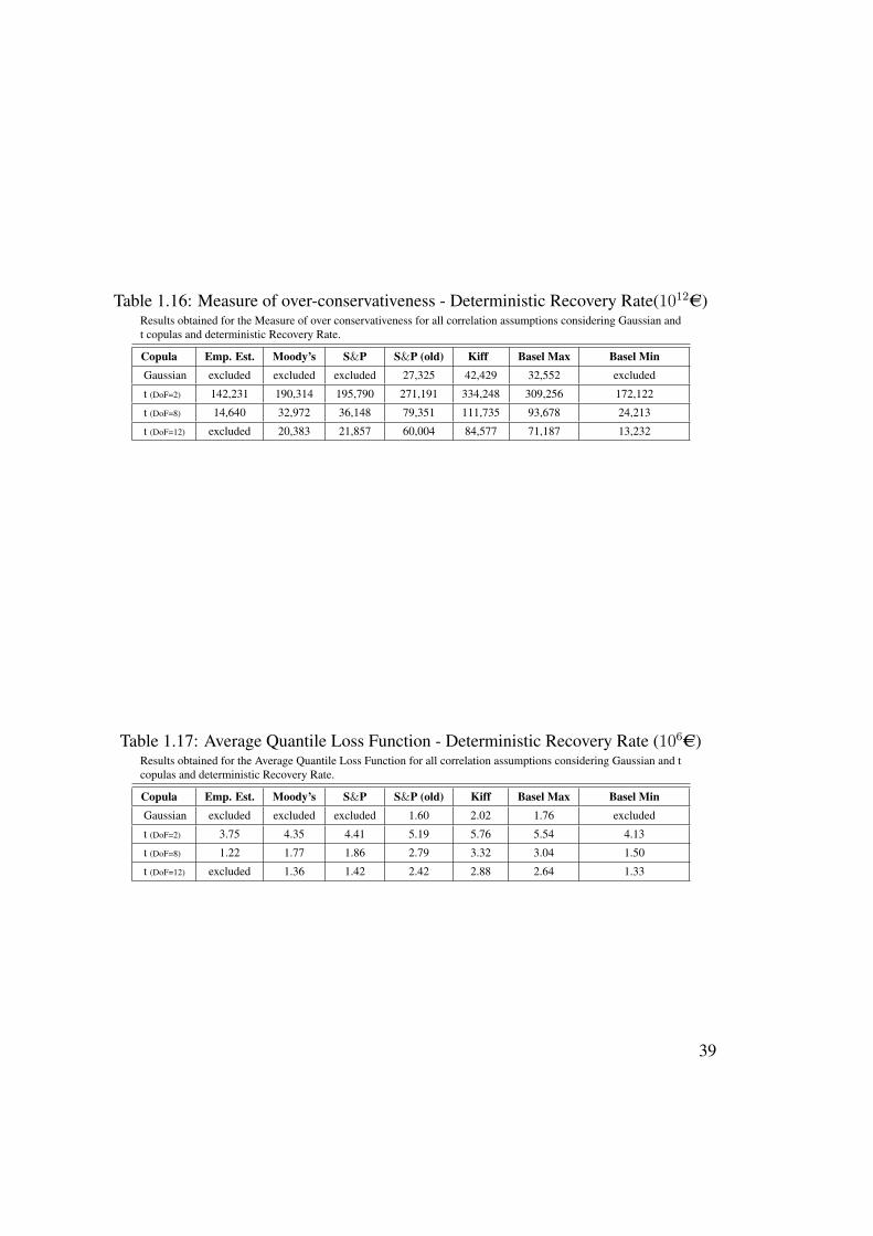
Table 1.16: Measure of over-conservativeness - Deterministic Recovery Rate(1012AC)Results obtained for the Measure of over conservativeness for all correlation assumptions considering Gaussian andt copulas and deterministic Recovery Rate.
Copula Emp. Est. Moody’s S&P S&P (old) Kiff Basel Max Basel MinGaussian excluded excluded excluded 27,325 42,429 32,552 excluded
t (DoF=2) 142,231 190,314 195,790 271,191 334,248 309,256 172,122
t (DoF=8) 14,640 32,972 36,148 79,351 111,735 93,678 24,213
t (DoF=12) excluded 20,383 21,857 60,004 84,577 71,187 13,232
Table 1.17: Average Quantile Loss Function - Deterministic Recovery Rate (106AC)Results obtained for the Average Quantile Loss Function for all correlation assumptions considering Gaussian and tcopulas and deterministic Recovery Rate.
Copula Emp. Est. Moody’s S&P S&P (old) Kiff Basel Max Basel MinGaussian excluded excluded excluded 1.60 2.02 1.76 excluded
t (DoF=2) 3.75 4.35 4.41 5.19 5.76 5.54 4.13
t (DoF=8) 1.22 1.77 1.86 2.79 3.32 3.04 1.50
t (DoF=12) excluded 1.36 1.42 2.42 2.88 2.64 1.33
39
Chapter 2
VaR in Credit Default Swaps
40
2.1 Literature Review
In recent years there have been several studies that propose different methods of cal-
culating VaR. Most of these studies focus on the calculation of VaR for stock returns.
The methods that have received most attention fall into four categories: nonparametric,
parametric, semi-parametric and hybrid. Among the parametric models, there is the
GARCH model proposed by Bollerslev (1986) and all the variants that have been intro-
duced, such as EGARCH proposed by Nelson (1991) and GJR model of Glosten et al
(1993). Concerning the semi-parametric models, Engle and Manganelli (2004) propose
a new approach to VaR estimation, the Conditional Autoregressive model (CAViaR),
which includes V aRt−1 as an explanatory variable. For a semi-parametric method,
Danielsson and De Vries (2000) propose the use of Extreme Value Theory for calcu-
lating VaR. Regarding the non parametric models, the most widely used are Historical
Simulation and Filtered Historical Simulation. McNeil and Frey (2000) analyze a hy-
brid model which combines GARCH with Extreme Value Theory.
The diversity of methods available to estimate VaR led to a wide range of studies that
provide empirical evidence of the performance of VaR approaches. Kuester et al (2006)
compare the out of sample performance of several methods of predicting univariate
VaR for the NASDAQ index and find that the hybrid method, combining a heavy-tailed
GARCH filter with an Extreme Value Theory-based approach, performs best overall,
closely followed by a variant on a Filtered Historical Simulation. They also find that
none of the CAViaR models tested performs adequately in all tests at any quantile level,
showing poor out of sample performance. Regarding the Mixture models, they conclude
that some of these models perform worse in smaller window sizes due presumably to
their rather large parameterizations and, for this reason, they are generally outperformed
by Filtered Historical Simulation and Extreme Value Theory.
Sener et al (2012) test and rank twelve different popular VaR methods on the equity
indices of eleven emerging and seven developed markets, covering the period of the re-
cent sub-prime mortgage crisis, and find that asymmetric methods, such as EGARCH,
generate the best performing VaR forecasts and the methods based in Extreme Value
Theory (EVT) approaches perform the worst. Rubia and Sanchis-Marco (2013) con-
sider the return-restricted CAViaR models originally proposed by Engle and Manganelli
41
(2004) as well as alternative models such as EVT and GARCH and use different vari-
ables which are related to measures of trading activity and liquidity. They find that
Quantile Regression-based risk models that account for the volatility and other market
conditions outperform the other approaches.
Rossignolo et al (2012) performs a comparative study of VaR models based on data
from emerging and frontier markets and find that Historical Simulation and Filtered His-
torical Simulation are inaccurate, conditional models represent an improvement, both
for GARCH and EGARCH techniques, and heavy tailed distributions, particularly EVT,
reveal as the most accurate technique to model market risk. A study performed by Hal-
bleib and Pohlmeier (2012), in which they propose the combination of different VaR
approaches to provide robust and precise VaR forecasts and provide empirical evidence
of the performance of a wide range of standard VaR approaches, supports the results
of Rossignolo et al (2012), as they also find that the best VaR approaches are based on
EVT.
The forecast of VaR in CDS requires, first, the estimation of the price of CDS in
the specific quantile of interest and then the calculation of VaR using a mark-to-market
technique. The key issue is the estimation of the price of the CDS in the tail of the price
distribution. For this purpose, the methods typically used to calculate VaR for stock
returns are applicable.
Considering the overall performance of Filtered Historical Simulation reported by
Kuester et al (2006) and the empirical evidence of the performance of Extreme Value
Theory reported in several of the recent studies presented above, I consider that these
are promising methods of estimating VaR and thus I will test them in this study. Follow-
ing Kuester et al (2006), I will also estimate VaR considering the Historical Simulation
method and GARCH models. In the analysis of Kuester et al (2006), the Mixture mod-
els present poor out of sample performance in small samples, which are the situations
of most interest in the evaluation of CDS due to their recent history, and for this reason
these models are not considered in this study.
There is a growing interest in employing Quantile Regression (QR) in the finance lit-
42
erature. QR was first applied to VaR estimation by Taylor (1999) and Chernozhukov and
Umantsev (2000). Taylor (1999) applies QR to estimate multiperiod VaR in the context
of exchange rates and compare this new approach with the traditional methods which
first estimate the volatility and then assume a probability distribution. Chernozhukov
and Umantsev (2000) use QR also to model VaR without, however, examining the per-
formance of this method.
Engle and Manganelli (2004) propose a particular specification for QR, called CAViaR.
Instead of modeling the whole distribution of returns, this model allows to concentrate
in the quantile directly and specify the evolution of the quantile over time using a special
type of autoregressive process. Chen et al (2012) propose a new family of VaR models
based on QR and find that these models consistently ranked best for VaR forecasting,
comparing to the classical approaches based on GARCH models.
Gebka and Wohar (2013) analyze the causality between past trading volumes and
index returns in the Pacific Basin countries and find that the QR method reveals strong
nonlinear causality even though this relation was not detected by OLS regression. Lee
and Li (2012) employ a QR approach and show that the effect of diversification on firm
performance is not homogeneous across various quantile levels. Baur (2013) proposes
an alternative framework to decompose the dependence using QR and demonstrates that
this methodology provides a detailed picture of dependence including asymmetric and
non-linear relationships. Allen et al (2012) apply QR to measure extreme risk of various
European industrial sectors both prior to and during the recent financial crisis and find a
highly significant difference in the distance to default between quantiles 50% and 95%.
Pires et al (2011) apply QR approach in order to model the distribution of CDS
spreads and, through the use of mark-to-market techniques, calculate VaR. Inspired by
the results of Pires et al (2011), in this study I also employ QR to identify the de-
terminants of CDS spreads in specific quantiles of interest, in order to calculate VaR.
However, I extend the results of Pires et al (2011) by augmenting the sample to include
the recent credit crisis and by testing additional explanatory variables.
The use of QR in the context of forecasting VaR is typically associated with differ-
ent specifications of the CAViaR model. However, in this study I use QR to identify the
determinants of the price of CDS and then calculate VaR, using mark-to-market tech-
43
niques. I compare the performance of the VaR model based on this specification of the
QR with the results obtained with Historical Simulation, Filtered Historical Simulation,
GARCH-based models and EVT, through the application of backtesting methodologies.
To the best of my knowledge this is the first time that backtesting methodologies are
applied to compare different methods of estimating VaR in CDS.
A wide range of macroeconomic and microeconomic factors have been analyzed in
the context of determinants of CDS spreads. Das et al (2009) compare the explana-
tory power of market-based and accounting-based models of CDS spreads and find that
models including both accounting and market information perform better than separate
models. Ericsson et al (2009) conclude that variables such as volatility and leverage,
which are theoretically implied variables, explain a significant proportion of CDS varia-
tions. Zhang et al (2005) analyze the impact of equity returns and volatility of the refer-
ence entity on the CDS premium and find that CDS spreads can be largely explained by
intra-day refined measures of historical volatility and jump probability. Bystrom (2005)
shows that CDS spreads are negatively correlated with stock prices and positively cor-
related with stock price volatility. Morkoetter et al (2012) show that counterparty de-
fault risk measures have a negative impact on CDS spreads. Regarding the measure of
counterparty default risk, Campbell et al (2008) find that financial ratios such as prof-
itability, leverage and liquidity play an important role in explaining the determinants of
bankruptcy and failure. Following these studies, I use market-based and accounting-
based factors as determinants of CDS spreads, namely stock returns and stock price
volatility and also financial ratios such as leverage, return on assets and liquidity.
Tang and Yan (2007) provide evidence that liquidity risk and liquidity level explain
a significant proportion of CDS spread variation. CDS liquidity, measured by absolute
bid ask spread, is introduced by Bongaerts et al (2011) and Pires et al (2011) as an
explanatory variable of CDS premiums. Pires et al (2011) find that CDS spreads sig-
nificantly increase with absolute bid ask spreads across all conditional quantiles of the
CDS distribution. Based on these results, in this study I use absolute bid ask spread as
a measure of CDS market liquidity.
44
2.2 CDS Price
2.2.1 Estimation Techniques
Banks and regulators are primarily interested in the aggregate VaR across trading ac-
tivities, raising the question of whether to start by aggregating the data and then apply
a univariate VaR model or to start with disaggregate data and then apply multivari-
ate structural portfolio VaR model. In evaluating the portfolio VaR, the multivariate
model can have some advantages over the univariate model. According to Bauwens et
al (2006), one of these advantages is that once we get the covariance matrix by the mul-
tivariate approach, we do not need to calculate again the covariance matrix even if the
weights of each asset are changed; under the univariate model, we should evaluate the
variance of portfolio again whenever the weights of each asset are changed. Another
advantage is that a multivariate model may improve the evaluation performance in up-
dating the variances and correlations by considering the individual characteristics of the
portfolios components and estimating their linear comovement. However, Berkowitz
and O’Brien (2002) show that the aggregation and modeling problems involved in the
multivariate approach may lead to poor forecasting accuracy and the simple univariate
model can even outperform these complicated structural models. Considering that uni-
variate models are a useful complement of the more complex structural models and may
even outperform these models and be sufficient for forecasting portfolio VaR, I restrict
attention to the univariate case.
A) Quantile Regression
The sensitivities to empirical determinants of CDS spreads may change according
to the level of CDS spread itself. Given this, a simple conditional mean regression may
not be appropriate to completely describe CDS spreads and in this case a more flexible
framework is required, for example the Quantile Regression.
The Quantile Regression was introduced by Koenker and Bassett (1978) and is an
extension of the conditional mean regression to a collection of models for different con-
ditional quantile functions.
45
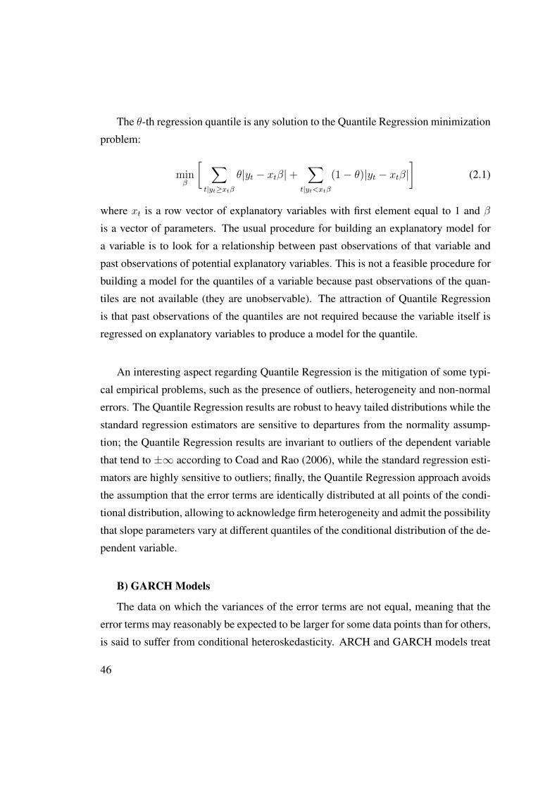
The θ-th regression quantile is any solution to the Quantile Regression minimization
problem:
minβ
[ ∑t|yt≥xtβ
θ|yt − xtβ|+∑
t|yt<xtβ
(1− θ)|yt − xtβ|]
(2.1)
where xt is a row vector of explanatory variables with first element equal to 1 and β
is a vector of parameters. The usual procedure for building an explanatory model for
a variable is to look for a relationship between past observations of that variable and
past observations of potential explanatory variables. This is not a feasible procedure for
building a model for the quantiles of a variable because past observations of the quan-
tiles are not available (they are unobservable). The attraction of Quantile Regression
is that past observations of the quantiles are not required because the variable itself is
regressed on explanatory variables to produce a model for the quantile.
An interesting aspect regarding Quantile Regression is the mitigation of some typi-
cal empirical problems, such as the presence of outliers, heterogeneity and non-normal
errors. The Quantile Regression results are robust to heavy tailed distributions while the
standard regression estimators are sensitive to departures from the normality assump-
tion; the Quantile Regression results are invariant to outliers of the dependent variable
that tend to ±∞ according to Coad and Rao (2006), while the standard regression esti-
mators are highly sensitive to outliers; finally, the Quantile Regression approach avoids
the assumption that the error terms are identically distributed at all points of the condi-
tional distribution, allowing to acknowledge firm heterogeneity and admit the possibility
that slope parameters vary at different quantiles of the conditional distribution of the de-
pendent variable.
B) GARCH Models
The data on which the variances of the error terms are not equal, meaning that the
error terms may reasonably be expected to be larger for some data points than for others,
is said to suffer from conditional heteroskedasticity. ARCH and GARCH models treat
46
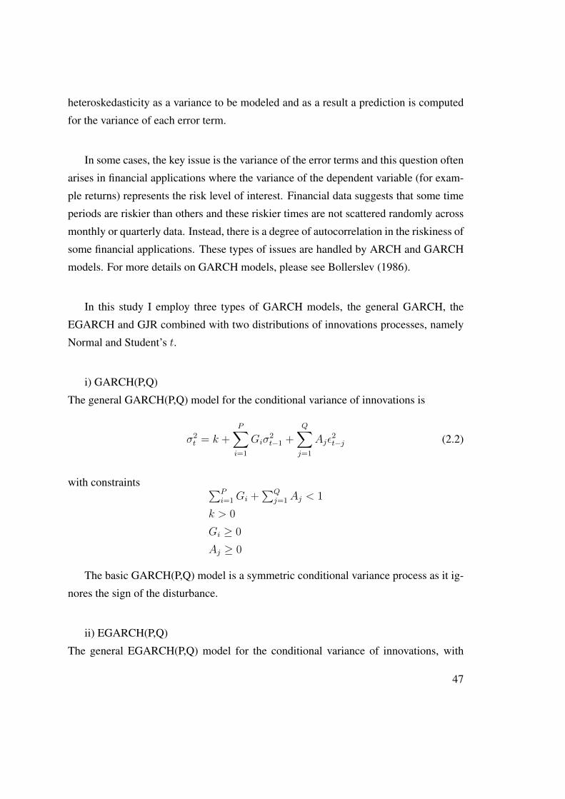
heteroskedasticity as a variance to be modeled and as a result a prediction is computed
for the variance of each error term.
In some cases, the key issue is the variance of the error terms and this question often
arises in financial applications where the variance of the dependent variable (for exam-
ple returns) represents the risk level of interest. Financial data suggests that some time
periods are riskier than others and these riskier times are not scattered randomly across
monthly or quarterly data. Instead, there is a degree of autocorrelation in the riskiness of
some financial applications. These types of issues are handled by ARCH and GARCH
models. For more details on GARCH models, please see Bollerslev (1986).
In this study I employ three types of GARCH models, the general GARCH, the
EGARCH and GJR combined with two distributions of innovations processes, namely
Normal and Student’s t.
i) GARCH(P,Q)
The general GARCH(P,Q) model for the conditional variance of innovations is
σ2t = k +
P∑i=1
Giσ2t−1 +
Q∑j=1
Ajε2t−j (2.2)
with constraints ∑Pi=1Gi +
∑Qj=1 Aj < 1
k > 0
Gi ≥ 0
Aj ≥ 0
The basic GARCH(P,Q) model is a symmetric conditional variance process as it ig-
nores the sign of the disturbance.
ii) EGARCH(P,Q)
The general EGARCH(P,Q) model for the conditional variance of innovations, with
47
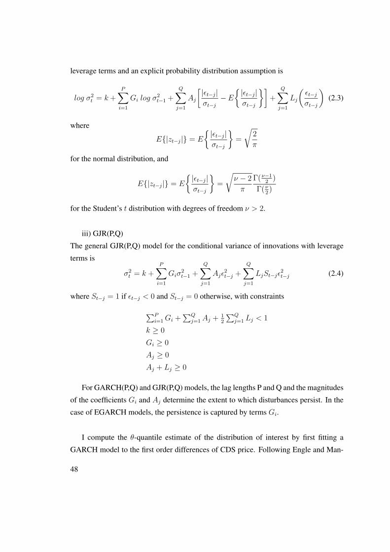
leverage terms and an explicit probability distribution assumption is
log σ2t = k +
P∑i=1
Gi log σ2t−1 +
Q∑j=1
Aj
[|εt−j|σt−j
−E|εt−j|σt−j
]+
Q∑j=1
Lj
(εt−jσt−j
)(2.3)
where
E|zt−j| = E
|εt−j|σt−j
=
√2
π
for the normal distribution, and
E|zt−j| = E
|εt−j|σt−j
=
√ν − 2
π
Γ(ν−12
)
Γ(ν2)
for the Student’s t distribution with degrees of freedom ν > 2.
iii) GJR(P,Q)
The general GJR(P,Q) model for the conditional variance of innovations with leverage
terms is
σ2t = k +
P∑i=1
Giσ2t−1 +
Q∑j=1
Ajε2t−j +
Q∑j=1
LjSt−jε2t−j (2.4)
where St−j = 1 if εt−j < 0 and St−j = 0 otherwise, with constraints
∑Pi=1 Gi +
∑Qj=1Aj + 1
2
∑Qj=1 Lj < 1
k ≥ 0
Gi ≥ 0
Aj ≥ 0
Aj + Lj ≥ 0
For GARCH(P,Q) and GJR(P,Q) models, the lag lengths P and Q and the magnitudes
of the coefficients Gi and Aj determine the extent to which disturbances persist. In the
case of EGARCH models, the persistence is captured by terms Gi.
I compute the θ-quantile estimate of the distribution of interest by first fitting a
GARCH model to the first order differences of CDS price. Following Engle and Man-
48
ganelli (1999), the one-period-ahead VaR estimate is calculated with following equa-
tion:
V aRt+1(θ) = µt+1 + σt+1Qθ(z) (2.5)
where µt+1 and σt+1 are the estimated conditional mean and conditional standard devi-
ation for t + 1, respectively, and Qθ(z) is the empirical θ-quantile of the standardized
residuals. In this study, I assume that the expected change in the CDS spread is zero. In
terms of equation 2.5, this corresponds to µt+1 = 0.
This estimation is a mix of a GARCH and a Historical Simulation applied to the
standardized residuals. Thus, whether the error distribution is conditional normal or
follows other distribution, it is straightforward to compute the one-step-ahead θ-quantile
forecast, since under all distributions we can compute the corresponding quantiles which
we then multiply by our conditional standard deviation forecast.
In order to estimate VaR for period t + h, I apply a simple scaling rule. Assuming
that µt+h = 0, this corresponds to multiplying the one-period-ahead estimated stan-
dard deviation by the square root of the number of periods ahead of the forecast (h),
according to the following equation:
V aRt+h(θ) =√hσt+1Qθ(z) (2.6)
C) Historical Simulation
The simplest way to estimate the θ-quantile of a distribution is to use the sample
quantile estimate based on historical data, which is referred to as Historical Simulation.
For Historical Simulation (HS), the θ-quantile estimate for t+1 is given by the empirical
θ-quantile, Qθ, of a moving window of w observations up to time t.
Despite being a popular way to estimate the θ-quantile of a particular distribution,
Historical Simulation has some major flaws. First, this method ignores the possible non-
iid nature of the data. Second, the length of the window one chooses must satisfy two
contradictory properties: it must be large enough in order to make statistical inference
significant and it must not be too large to avoid the risk of taking observations outside of
the current volatility cluster. Finally, when the market moves from a period of relatively
low volatility to a period of relatively high volatility (or vice versa), θ-quantile estimates
49
based on Historical Simulation will be biased downward (upward).
A variant of the Historical Simulation method presented above is the Filtered His-
torical Simulation (FHS), which has shown very good results in the study performed by
Kuester et al (2006). For FHS, a GARCH model is used to prefilter the data and the
nonparametric nature of Historical Simulation is retained by bootstrapping (sampling
with replacement) from the standardized residuals. These bootstrapped standardized
residuals are then used to generate time paths of future CDS prices. One of the appeal-
ing features of FHS is its ability to generate relatively large deviations not found in the
original time series.
D) Extreme Value Theory
Extreme value theory (EVT) focuses on the tails of the distribution of interest. Fol-
lowing Diebold et al (1998), in this study I fit a time-varying model to the data and then
estimate the tail of the standardized residuals by an EVT model, using the limit result
for peaks over threshold (POT). This process first extracts the filtered residuals from
each series with a GARCH model, then constructs the sample marginal cumulative dis-
tribution function of each asset using a Gaussian kernel estimate for the interior and a
generalized Pareto distribution estimate for the tails.
McNeil and Frey (2000) combine an AR(1)-GARCH(1,1) process, assuming normal
innovations, with the POT method. The filter with normal innovations is capable of re-
moving the majority of clusterings and for this reason I also assume normal innovations
in this study.
The one-day-ahead VaR estimate is given by equation 2.5, where µt+1 and σt+1 are
the estimated conditional mean and conditional standard deviation for t + 1, respec-
tively, obtained from a AR(1)-GARCH(1,1) process. Moreover, Qθ(z) is the θ-quantile
estimate of the standardized residuals, obtained with the POT method. The estimation
of VaR for period t + h is given by equation 2.6. I refer to Embrechts et al (1997) for
more details on EVT.
50
2.2.2 VaR Estimation
The value at risk measure places an upper bound on losses in the sense that these will
exceed the VaR threshold with a small target probability, typically chosen between 1%
and 5%. Conditional on the information given up to time t, the VaR for period t+h at
the confidence level θ is given by:
V aRθt+h := Qθ(L|Xt) = infl ∈ R : P (L > l|Xt) ≤ 1− θ, 0 < θ < 1 (2.7)
where Qθ(.) denotes que quantile function, L is the loss in period t and Xt represents
the information available at date t. For implementing VaR based measures, one seeks
a precise quantile estimate relatively far out in the right tail of the loss distribution for
some specified future date.
The estimation methods described in the previous section are used to estimate the
price of a CDS in time period t, with a certain confidence level, meaning that the output
of these estimation methods will be a price for the CDS. The price evolution of CDS
allows us to understand the evolution of the risk of the underlying entity and compare
the predicted price with the price observed in the market. Thus, by examining the price
of CDS over time we can compare different estimation methods and analyze their ac-
curacy, but the price of CDS alone does not provide a loss distribution and a Value at
Risk. To transform the distribution of CDS spreads into a distribution of losses I use
the reduced-form model described in O’Kane and Turnbull (2003). This transformation
allows us to convert basis points into monetary values, thus allowing the calculation of
Value at Risk.
Following O’Kane and Turnbull (2003), unlike bonds the gain or loss from a CDS
position cannot be computed simply by taking the difference between current market
quoted price plus the coupons received and the purchase price. To value a CDS we need
to use a term structure of default swap spreads, a recovery rate assumption and a model.
The present value of a position initially traded at time t0 at a contractual spread of
S(to, tN) with maturity tN and which has been offset at valuation time tV with a position
51
traded at a spread of S(tV , tN) is given by:
MTM(S(to, tN), λ) = ±[S(tV , tN)− S(to, tN)]×RPV 01(tV , tN) (2.8)
where
RPV 01 =N∑n=1
Z(tn) ·∆tn[Q(tn) +
(Q(tn−1)−Q(tn)
)· 1pa
2
](2.9)
denotes the Risky present value of 1 bp paid on the premium leg, the indicator 1pa
equals 1 if the contract specifies premium accrued and 0 otherwise, ∆tn is the number
of years between payment dates, Z(tn) is the risk-free discount factor for tn (e−rtn),
Q(tn) = e−λtn is the probability of survival until tn and λ is the hazard rate. The
positive sign is used for the protection buyer and the negative sign for the protection
seller.
Following Pires et al (2011), I assume a flat recovery rate (R) of 40% and a flat
interest rate (r) of 5%. The approximate break-even flat hazard rate is computed as:
λ =S
(1−R)
Let Si,t denote the CDS spread for entity i at time t and λθ =F−1Si,t
(θ|Xi,t)
(1−R)denote
the hazard rate for the estimated CDS price at a given quantile θ. The value at risk is
computed as:
V aRθ(Si,t|Xi,t) = MTM(Si,t, λθ)
The Value at Risk represents the change in value of a contract initially negotiated at
price Si,t due to a change in the hazard rate to λθ. This new hazard rate represents a
new CDS spread at a given quantile θ. Different methods of CDS price estimation will
lead to potentially different price estimates at a given quantile θ, i.e., each estimation
technique will be associated with a specific λθ for the time t and firm i. Assuming
that I am a protection seller, I am interested in the risk of the CDS spread increasing.
Therefore, I will focus on the forecast of upper quantiles of the price of CDS, namely
quantile 99.
52
2.3 Backtesting VaR
The Value at Risk represents the change in value of a contract initially negotiated at price
Si,t due to a change in the hazard rate to λθ. However, the real change in the hazard rate
observed in the market in a specific time interval might be higher or lower, meaning that
the real mark-to-market might be higher or lower than predicted by the VaR model. For
this reason, the backtesting will be performed by comparing the estimated VaR with the
real mark-to-market considering the implicit hazard rate of the maximum price that the
CDS reached in the following 1, 3, 10 and 30 days, allowing us to check the accuracy
of VaR estimates with a time horizon of 1, 3, 10 and 30 days.
The backtesting of VaR methods in CDS will be performed based on the tests pre-
sented in chapter 1 and two additional tests, namely Conditional Tail Expectation and
Dynamic Quantile Test, which I present in the following.
A) Conditional Tail Expectation
Artzner et al (1999) present Conditional Tail Expectation as a measure of risk de-
fined by:
CTEθ(X) = E[xt,t+1|xt,t+1 > V aRt(θ)] (2.10)
The CTE measure should be interpreted carefully and should be examined in con-
junction with other methods of backtesting, such as the Average Quantile Loss, because
the value of the loss observed when there is a violation of VaR gives an idea of the
severity of the loss but gives no indication of the closeness between the loss and the
VaR estimate, i.e., there may be a violation of VaR and loss observed may be extremely
high, and yet, the estimated VaR is very close to the observed loss.
B) Dynamic Quantile Test
Engle and Manganelli (2004) propose a test based on the regression of It on a re-
53
gressor matrix X that contains lagged hits, It−1,...,It−p, for example:
It = θ0 +
p∑i=1
βiIt−i + µt, (2.11)
where, under the null hypothesis, θ0 = θ and βi = 0, i = 1, ...p. In vector notation, we
have:
I − θι = Xβ + µ (2.12)
where ι is a vector of ones.
Invoking the central limit theorem yields
βLS = (X ′X)−1X ′(I − θι) asy∼ N(0, (X ′X)−1θ(1− θ)
)(2.13)
The DQ test consists in testing some linear restrictions in a linear model that links the
violations to a set of explanatory variables. Tests such as the proposed by Christoffersen
(1998) can detect the presence of serial correlation in the sequence of indicator functions
but this is only a necessary but not sufficient condition to assess the performance of a
quantile model because, in some situations, the unconditional probabilities of exceeding
the quantile are correct and serially uncorrelated but the conditional probabilities given
the quantile are not. The tests presented above have no power against this form of
inefficiency.
Considering that the empirical application in this study covers CDS with short his-
tory and in order to minimize the loss of information,the regressor matrix X contains
the constant and two lagged hits.
2.4 Empirical Analysis
2.4.1 Data Sample
I use the Bloomberg Financial Services database to obtain all the names that belonged
to any of the first 16 series of two important CDS indexes for the US market: the CDX
North America Investment Grade and the CDX North America High Yield. I restrict
54
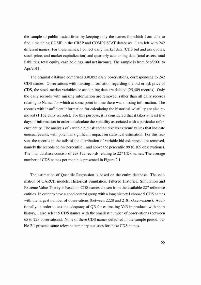
the sample to public traded firms by keeping only the names for which I am able to
find a matching CUSIP in the CRSP and COMPUSTAT databases. I am left with 242
different names. For these names, I collect daily market data (CDS bid and ask quotes,
stock price, and market capitalization) and quarterly accounting data (total assets, total
liabilities, total equity, cash holdings, and net income). The sample is from Sep/2001 to
Apr/2011.
The original database comprises 330,852 daily observations, corresponding to 242
CDS names. Observations with missing information regarding the bid or ask price of
CDS, the stock market variables or accounting data are deleted (25,409 records). Only
the daily records with missing information are removed, rather than all daily records
relating to Names for which at some point in time there was missing information. The
records with insufficient information for calculating the historical volatility are also re-
moved (1,162 daily records). For this purpose, it is considered that it takes at least five
days of information in order to calculate the volatility associated with a particular refer-
ence entity. The analysis of variable bid ask spread reveals extreme values that indicate
unusual events, with potential significant impact on statistical estimation. For this rea-
son, the records in the tails of the distribution of variable bid ask spread are removed,
namely the records below percentile 1 and above the percentile 99 (6,109 observations).
The final database consists of 298,172 records relating to 227 CDS names. The average
number of CDS names per month is presented in Figure 2.1.
The estimation of Quantile Regression is based on the entire database. The esti-
mation of GARCH models, Historical Simulation, Filtered Historical Simulation and
Extreme Value Theory is based on CDS names chosen from the available 227 reference
entities. In order to have a good control group with a long history I choose 5 CDS names
with the largest number of observations (between 2228 and 2181 observations). Addi-
tionally, in order to test the adequacy of QR for estimating VaR in products with short
history, I also select 5 CDS names with the smallest number of observations (between
65 to 223 observations). None of these CDS names defaulted in the sample period. Ta-
ble 2.1 presents some relevant summary statistics for these CDS names.
55
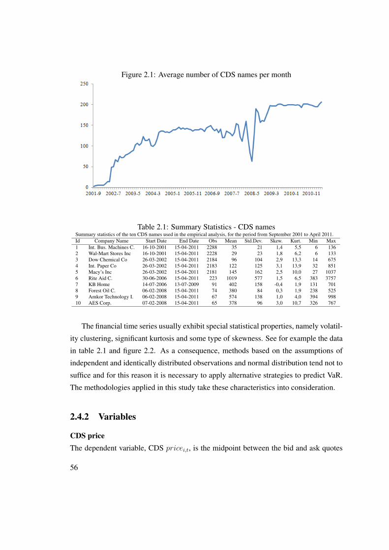
Figure 2.1: Average number of CDS names per month
Table 2.1: Summary Statistics - CDS namesSummary statistics of the ten CDS names used in the empirical analysis, for the period from September 2001 to April 2011.Id Company Name Start Date End Date Obs Mean Std.Dev. Skew. Kurt. Min Max1 Int. Bus. Machines C. 16-10-2001 15-04-2011 2288 35 21 1,4 5,5 6 1362 Wal-Mart Stores Inc 16-10-2001 15-04-2011 2228 29 23 1,8 6,2 6 1333 Dow Chemical Co 26-03-2002 15-04-2011 2184 96 104 2,9 13,3 14 6754 Int. Paper Co 26-03-2002 15-04-2011 2183 122 125 3,1 13,9 32 8515 Macy’s Inc 26-03-2002 15-04-2011 2181 145 162 2,5 10,0 27 10376 Rite Aid C. 30-06-2006 15-04-2011 223 1019 577 1,5 6,5 383 37577 KB Home 14-07-2006 13-07-2009 91 402 158 -0,4 1,9 131 7018 Forest Oil C. 06-02-2008 15-04-2011 74 380 84 0,3 1,9 238 5259 Amkor Technology I. 06-02-2008 15-04-2011 67 574 138 1,0 4,0 394 99810 AES Corp. 07-02-2008 15-04-2011 65 378 96 3,0 10,7 326 767
The financial time series usually exhibit special statistical properties, namely volatil-
ity clustering, significant kurtosis and some type of skewness. See for example the data
in table 2.1 and figure 2.2. As a consequence, methods based on the assumptions of
independent and identically distributed observations and normal distribution tend not to
suffice and for this reason it is necessary to apply alternative strategies to predict VaR.
The methodologies applied in this study take these characteristics into consideration.
2.4.2 Variables
CDS priceThe dependent variable, CDS pricei,t, is the midpoint between the bid and ask quotes
56
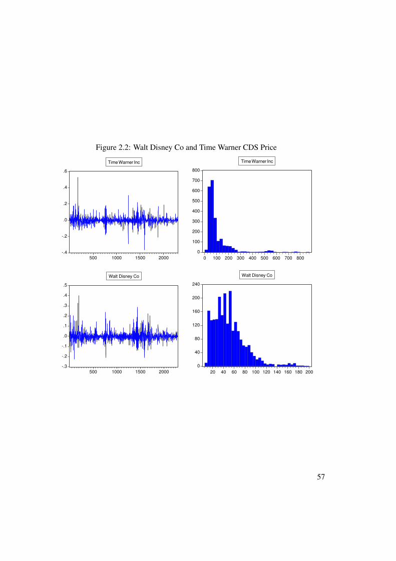
Figure 2.2: Walt Disney Co and Time Warner CDS Price
-.4
-.2
.0
.2
.4
.6
500 1000 1500 2000
Time Warner Inc
0
100
200
300
400
500
600
700
800
0 100 200 300 400 500 600 700 800
Series: CDS_PRICE
Sample 1 2305
Observations 2305
Mean 100.5086
Median 64.11650
Maximum 872.5000
Minimum 18.92750
Std. Dev. 108.3639
Skewness 3.523347
Kurtosis 17.54468
Jarque-Bera 25086.42
Probability 0.000000
Time Warner Inc
-.3
-.2
-.1
.0
.1
.2
.3
.4
.5
500 1000 1500 2000
Walt Disney Co
0
40
80
120
160
200
240
20 40 60 80 100 120 140 160 180 200
Series: CDS_PRICE
Sample 1 2299
Observations 2299
Mean 50.58967
Median 44.95400
Maximum 195.6250
Minimum 9.380500
Std. Dev. 30.05849
Skewness 1.413301
Kurtosis 6.060805
Jarque-Bera 1662.772
Probability 0.000000
Walt Disney Co
57
for firm i and period t.
Stock returnPositive equity returns increase the value of equity and therefore diminish the leverage
of the firm. Accordingly, it is expected that the CDS quote is negatively impacted by
equity returns.
Volatility of stock returnsHigher firm-specific equity volatility indicates a higher probability that the firm’s value
will cross the threshold of default, hence increasing CDS quotes. In this study historical
volatility is computed as:
Historical volatilityt =
√√√√252× 1
n− 1×
t−1∑i=t−31
r2i , (2.14)
Where ri is the daily stock return.
Bid ask spreadThe standard measure of liquidity for stocks and bonds is the relative bid ask spread.
However, contrary to stock prices, CDS premiums are expressed in comparable units:
basis points per annum of the notional amount of the contract. Pires et al (2011) provide
examples that give intuition that dividing the CDS bid ask spread by the CDS mid quote
can bias the comparison of liquidity between different reference entities. Based on this
reasoning, absolute rather than relative bid ask spread is used as independent variable.
LeverageAccording to Merton (1974), a firm defaults if the value of its assets falls below the
value of its debt and, hence, the leverage ratio is crucial for determining the distance
to default. In other words, an increase in leverage results in an increased probability of
default and consequently in an increase of the CDS premiums. Following Campbell et
al (2008), the leverage ratio of the reference entity is computed considering the book
value and also the market value of equity. The ratio is defined as:
58
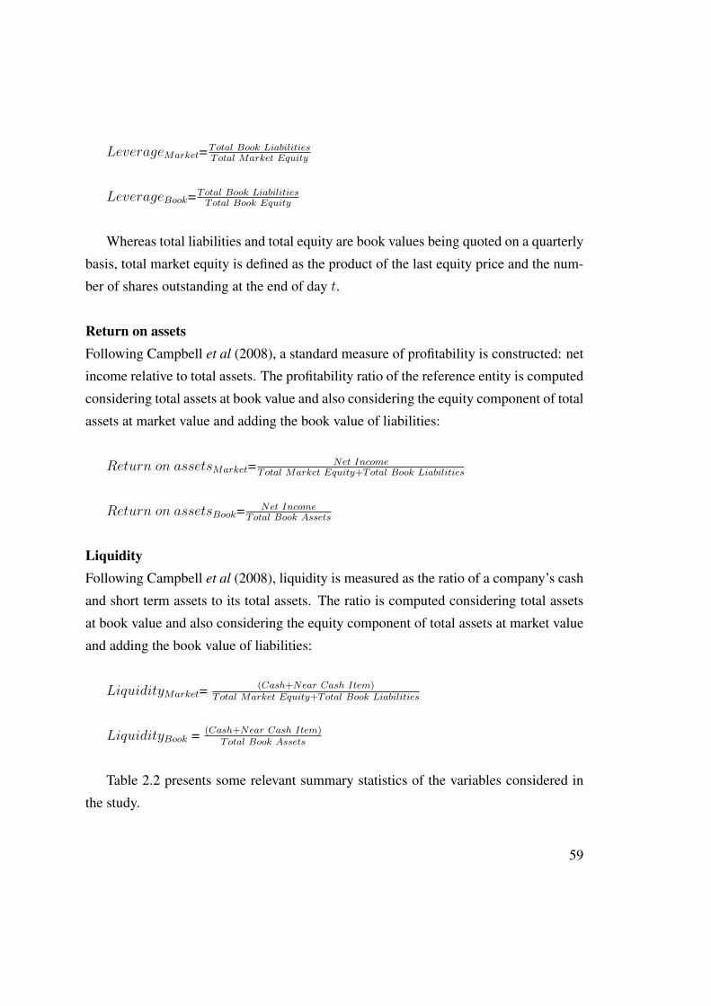
LeverageMarket=Total Book LiabilitiesTotal Market Equity
LeverageBook=Total Book LiabilitiesTotal Book Equity
Whereas total liabilities and total equity are book values being quoted on a quarterly
basis, total market equity is defined as the product of the last equity price and the num-
ber of shares outstanding at the end of day t.
Return on assetsFollowing Campbell et al (2008), a standard measure of profitability is constructed: net
income relative to total assets. The profitability ratio of the reference entity is computed
considering total assets at book value and also considering the equity component of total
assets at market value and adding the book value of liabilities:
Return on assetsMarket= Net IncomeTotal Market Equity+Total Book Liabilities
Return on assetsBook= Net IncomeTotal Book Assets
LiquidityFollowing Campbell et al (2008), liquidity is measured as the ratio of a company’s cash
and short term assets to its total assets. The ratio is computed considering total assets
at book value and also considering the equity component of total assets at market value
and adding the book value of liabilities:
LiquidityMarket=(Cash+Near Cash Item)
Total Market Equity+Total Book Liabilities
LiquidityBook = (Cash+Near Cash Item)Total Book Assets
Table 2.2 presents some relevant summary statistics of the variables considered in
the study.
59
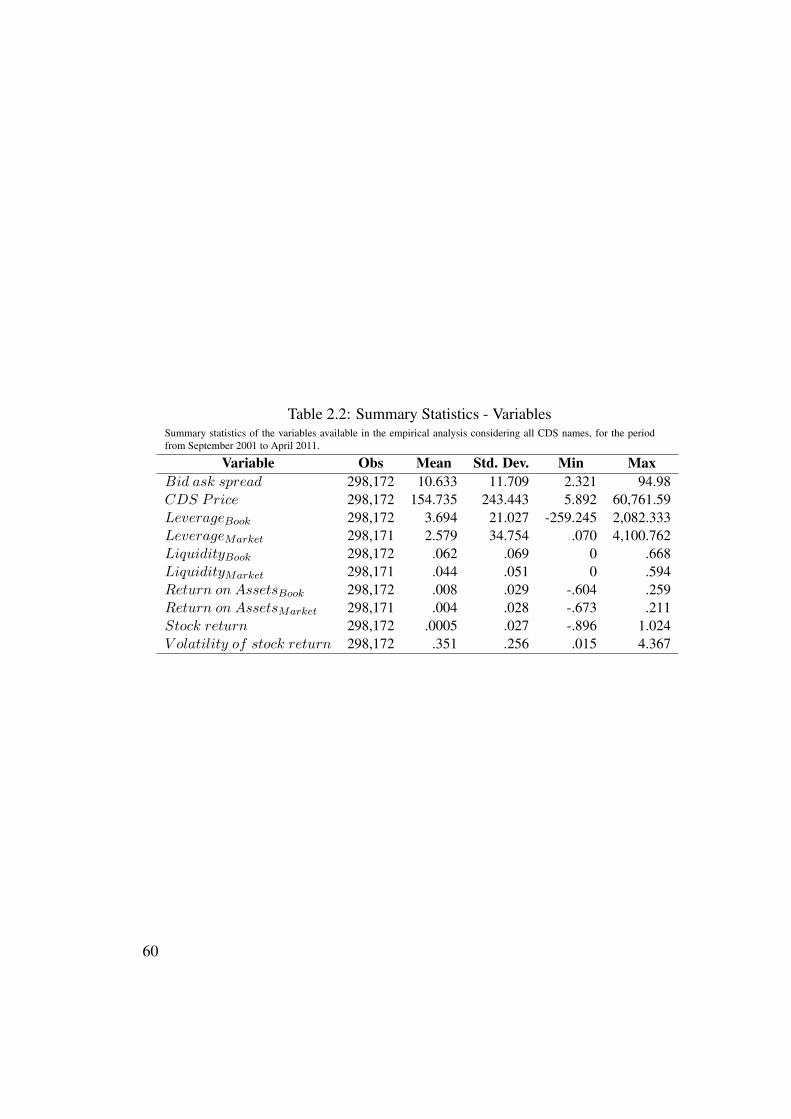
Table 2.2: Summary Statistics - VariablesSummary statistics of the variables available in the empirical analysis considering all CDS names, for the periodfrom September 2001 to April 2011.
Variable Obs Mean Std. Dev. Min MaxBid ask spread 298,172 10.633 11.709 2.321 94.98CDS Price 298,172 154.735 243.443 5.892 60,761.59LeverageBook 298,172 3.694 21.027 -259.245 2,082.333LeverageMarket 298,171 2.579 34.754 .070 4,100.762LiquidityBook 298,172 .062 .069 0 .668LiquidityMarket 298,171 .044 .051 0 .594Return on AssetsBook 298,172 .008 .029 -.604 .259Return on AssetsMarket 298,171 .004 .028 -.673 .211Stock return 298,172 .0005 .027 -.896 1.024V olatility of stock return 298,172 .351 .256 .015 4.367
60
2.4.3 CDS Price Estimation1
A) Quantile Regression
A panel data analysis is performed to determine the impact of cross-sectional and
time-series variables on CDS spreads. In order to identify variables which generally
contribute most to explain the price of CDS, I start by estimating a linear regression
suitable for panel data for the entire database, considering all independent variables
available, in particular, information regarding the CDS (bid ask spread), information on
the share price of the company (total stock return, stock volatility) and economic and
financial information of the company (return on assets, leverage and liquidity).
To obtain efficient results I test whether the variables exhibit autocorrelation by the
Lagrange multiplier test (Wooldridge (2002)). The test shows evidence of the presence
of autocorrelation, which causes the standard errors of the coefficients to be smaller
than they actually are and higher R-squared. Based on a Hausman test, a fixed-effects
model is specified for the analysis of the determinants of CDS spreads for the regression
model. In order to test for the presence of heteroskedasticity, that is, the error terms
µi,t do not have constant variance for firm i and time period t, a modified Wald test
for groupwise heteroskedasticity in fixed effects regression model is performed with
the null hypothesis that the variance of one group j equals the overall variance (σ2j =
σ2overall). The null hypothesis is rejected. Considering that there is evidence of the
presence of autocorrelation and heteroskedasticity, it is applied a robust estimator of the
error variance matrix against both heteroskedasticity and autocorrelation.
To check whether time fixed effects are needed when estimating the fixed-effects
model, I include time dummies for each period in the regression model and, based on
the F-test, I conclude that time fixed effects are needed. Taking into account these ad-
justments, the different specifications for the financial ratios based on book values and
market values of equity, and the other variables available, several alternative specifi-
cations for the regression are tested. The variables that show statistical significance
and economic intuition in explaining the determinants of the price of the CDS with the
highest explanatory power are: bid ask spread, the stock return, the volatility of stock
1Linear Regression and Quantile Regression for panel data were estimated with the software Stata.The remaining models were estimated with the software Matlab.
61
returns, return on assets and leverage, both based on the book value of equity, and time
dummies.The regression model is designed as:
CDS spreadi,t = β1bid ask spreadi,t + β2stock returni,t
+β3stock volatilityi,t + β4return on assetsBooki,t
+β7leverageBooki,t
+ai + at + µi,t
With ai and at representing entity-fixed and time-fixed effects.
Regarding overall goodness of fit, the high F-statistics indicates that all model pa-
rameters are different from zero and the R2 value is 53.8%. Table 2.3 presents the
results.
Comparing with the results obtained in Campbell et al (2008), I conclude that some
of the predictor variables of failure are important to explain the CDS prices but there
are some differences. In the study performed by Campbell et al (2008), the profitability
and leverage ratios that perform better are those that measure the equity component of
total assets at market value, while in this study the ratios that perform better are based
on the book value of equity. Additionally, in Campbell et al (2008) the liquidity ratio is
statistically significant and has a coefficient according to the economic intuition but in
this study these conditions are not verified.
The estimation of linear panel models is a starting point to identify the variables
that contribute most to explain the determinants of the price of CDS and understand the
characteristics of the data. However, the main interest of this study is to identify the
determinants of the price of CDS in a specific quantile and, therefore, I proceed to the
estimation of Quantile Regression. Table 2.4 presents the results obtained with Quantile
Regression, for the 99 quantile, considering robust standard error estimation based on
bootstrap methods.
62
The Quantile Regression presented in table 2.4 is estimated considering all the avail-
able sampling window, i.e., the application of this equation for determining the price of
CDS at time period t will be performed based on parameters estimated on a sample
that considers periods after t. To minimize the problem of estimating the price of CDS
based on information that is not yet available at the time, I estimate a new regression in
each period considering only the information available at that time. In each subsequent
period, the new information available is added to the previous sampling window and a
new estimation of Quantile Regression is performed. Taking into account, on the one
hand, the importance of having a database sufficiently representative of the determinants
of the price of CDS and, second, that since the financial crisis in 2008 there has been
a sudden increase in the price of the CDS, the first regression is performed considering
the period 2001-2008 and from that date new regressions are estimated for each month
until April 2011. The estimation of VaR and its backtesting will be made based on the
monthly regressions, whose results are presented in the appendix. Comparing the results
obtained in each monthly regression over time, I find that the coefficient of the variable
bid ask spread has increased in each monthly regression, opposed to the reduction in the
absolute value of the coefficients of the variables stock volatility, return on assets and
leverage. This change in the monthly regression coefficients reflects an increase in the
contribution of bid ask spread to explain the price of CDS in the 99th percentile.
B) GARCH Models
The original time series are not stationary as can be seen by the results of the Dickey-
Fuller test presented in table 2.5. In order to transform the original time series into sta-
tionary series, I apply first order differences. The time series are modeled with three
types of GARCH models, the GARCH(1,1), the EGARCH(1,1) and GJR(1,1), com-
bined with two distributions of innovations processes, namely Normal and Students’s
t.
The estimation of GARCH models considering all the available sampling window
followed by the application of these equations for determining the price of CDS at time
period t would be performed based on parameters estimated on a sample that considers
periods after t. For this reason, in line with the procedure followed for Quantile Regres-
63
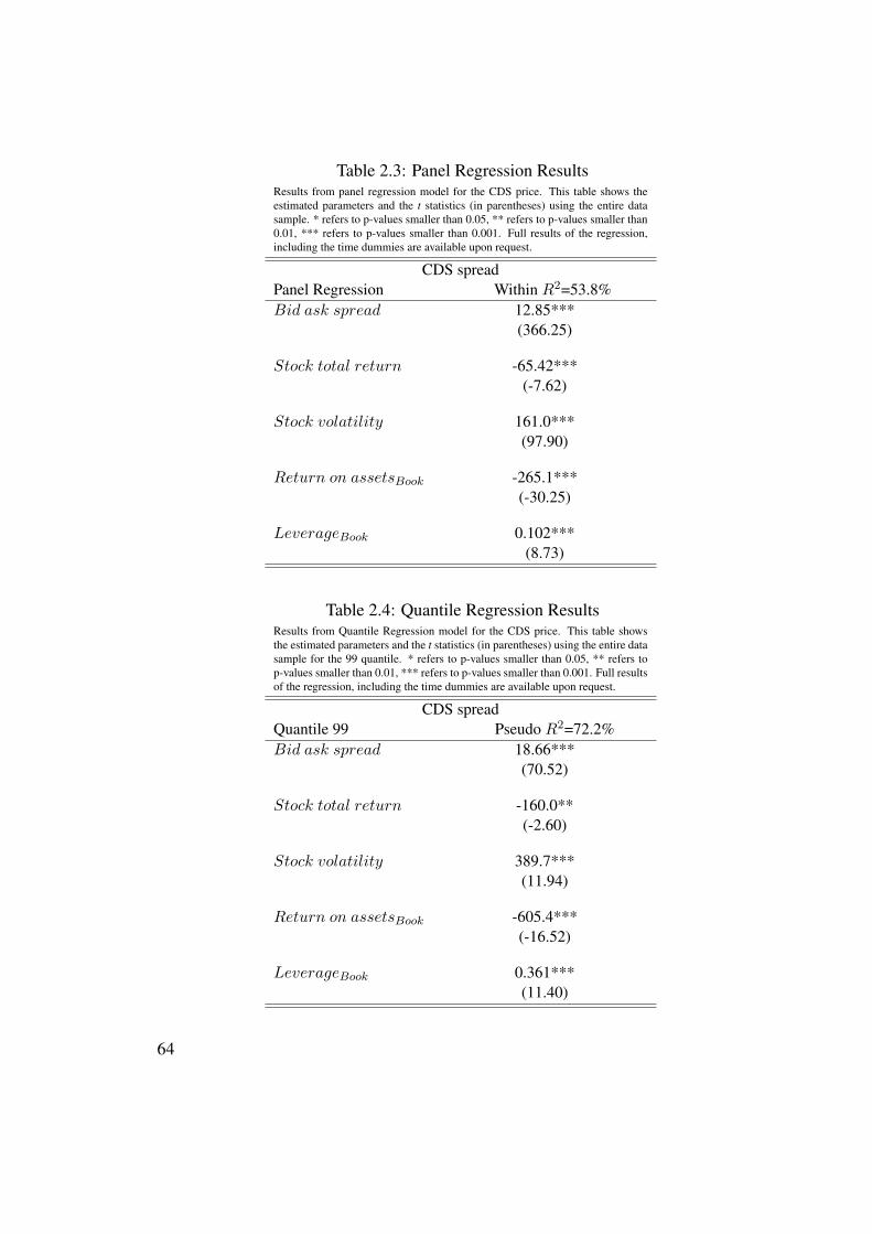
Table 2.3: Panel Regression ResultsResults from panel regression model for the CDS price. This table shows theestimated parameters and the t statistics (in parentheses) using the entire datasample. * refers to p-values smaller than 0.05, ** refers to p-values smaller than0.01, *** refers to p-values smaller than 0.001. Full results of the regression,including the time dummies are available upon request.
CDS spreadPanel Regression Within R2=53.8%Bid ask spread 12.85***
(366.25)
Stock total return -65.42***(-7.62)
Stock volatility 161.0***(97.90)
Return on assetsBook -265.1***(-30.25)
LeverageBook 0.102***(8.73)
Table 2.4: Quantile Regression ResultsResults from Quantile Regression model for the CDS price. This table showsthe estimated parameters and the t statistics (in parentheses) using the entire datasample for the 99 quantile. * refers to p-values smaller than 0.05, ** refers top-values smaller than 0.01, *** refers to p-values smaller than 0.001. Full resultsof the regression, including the time dummies are available upon request.
CDS spreadQuantile 99 Pseudo R2=72.2%Bid ask spread 18.66***
(70.52)
Stock total return -160.0**(-2.60)
Stock volatility 389.7***(11.94)
Return on assetsBook -605.4***(-16.52)
LeverageBook 0.361***(11.40)
64
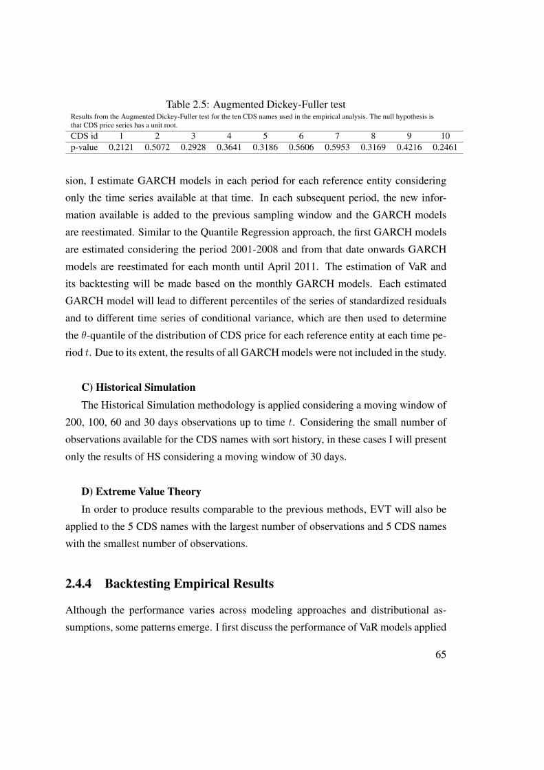
Table 2.5: Augmented Dickey-Fuller testResults from the Augmented Dickey-Fuller test for the ten CDS names used in the empirical analysis. The null hypothesis isthat CDS price series has a unit root.
CDS id 1 2 3 4 5 6 7 8 9 10p-value 0.2121 0.5072 0.2928 0.3641 0.3186 0.5606 0.5953 0.3169 0.4216 0.2461
sion, I estimate GARCH models in each period for each reference entity considering
only the time series available at that time. In each subsequent period, the new infor-
mation available is added to the previous sampling window and the GARCH models
are reestimated. Similar to the Quantile Regression approach, the first GARCH models
are estimated considering the period 2001-2008 and from that date onwards GARCH
models are reestimated for each month until April 2011. The estimation of VaR and
its backtesting will be made based on the monthly GARCH models. Each estimated
GARCH model will lead to different percentiles of the series of standardized residuals
and to different time series of conditional variance, which are then used to determine
the θ-quantile of the distribution of CDS price for each reference entity at each time pe-
riod t. Due to its extent, the results of all GARCH models were not included in the study.
C) Historical SimulationThe Historical Simulation methodology is applied considering a moving window of
200, 100, 60 and 30 days observations up to time t. Considering the small number of
observations available for the CDS names with sort history, in these cases I will present
only the results of HS considering a moving window of 30 days.
D) Extreme Value TheoryIn order to produce results comparable to the previous methods, EVT will also be
applied to the 5 CDS names with the largest number of observations and 5 CDS names
with the smallest number of observations.
2.4.4 Backtesting Empirical Results
Although the performance varies across modeling approaches and distributional as-
sumptions, some patterns emerge. I first discuss the performance of VaR models applied
65
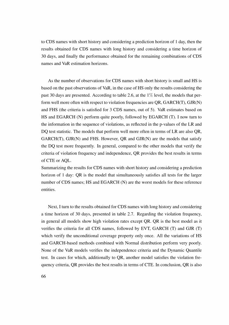
to CDS names with short history and considering a prediction horizon of 1 day, then the
results obtained for CDS names with long history and considering a time horizon of
30 days, and finally the performance obtained for the remaining combinations of CDS
names and VaR estimation horizons.
As the number of observations for CDS names with short history is small and HS is
based on the past observations of VaR, in the case of HS only the results considering the
past 30 days are presented. According to table 2.6, at the 1% level, the models that per-
form well more often with respect to violation frequencies are QR, GARCH(T), GJR(N)
and FHS (the criteria is satisfied for 3 CDS names, out of 5). VaR estimates based on
HS and EGARCH (N) perform quite poorly, followed by EGARCH (T). I now turn to
the information in the sequence of violations, as reflected in the p-values of the LR and
DQ test statistic. The models that perform well more often in terms of LR are also QR,
GARCH(T), GJR(N) and FHS. However, QR and GJR(N) are the models that satisfy
the DQ test more frequently. In general, compared to the other models that verify the
criteria of violation frequency and independence, QR provides the best results in terms
of CTE or AQL.
Summarizing the results for CDS names with short history and considering a prediction
horizon of 1 day: QR is the model that simultaneously satisfies all tests for the larger
number of CDS names; HS and EGARCH (N) are the worst models for these reference
entities.
Next, I turn to the results obtained for CDS names with long history and considering
a time horizon of 30 days, presented in table 2.7. Regarding the violation frequency,
in general all models show high violation rates except QR. QR is the best model as it
verifies the criteria for all CDS names, followed by EVT, GARCH (T) and GJR (T)
which verify the unconditional coverage property only once. All the variations of HS
and GARCH-based methods combined with Normal distribution perform very poorly.
None of the VaR models verifies the independence criteria and the Dynamic Quantile
test. In cases for which, additionally to QR, another model satisfies the violation fre-
quency criteria, QR provides the best results in terms of CTE. In conclusion, QR is also
66
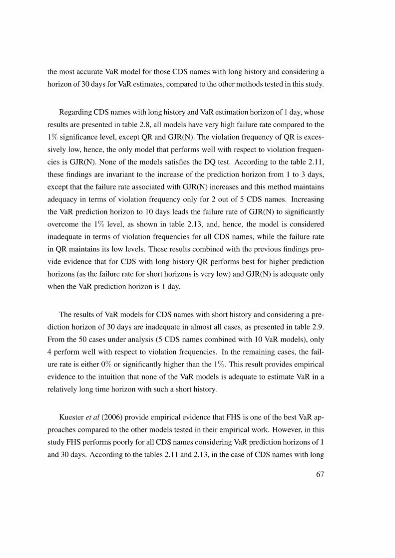
the most accurate VaR model for those CDS names with long history and considering a
horizon of 30 days for VaR estimates, compared to the other methods tested in this study.
Regarding CDS names with long history and VaR estimation horizon of 1 day, whose
results are presented in table 2.8, all models have very high failure rate compared to the
1% significance level, except QR and GJR(N). The violation frequency of QR is exces-
sively low, hence, the only model that performs well with respect to violation frequen-
cies is GJR(N). None of the models satisfies the DQ test. According to the table 2.11,
these findings are invariant to the increase of the prediction horizon from 1 to 3 days,
except that the failure rate associated with GJR(N) increases and this method maintains
adequacy in terms of violation frequency only for 2 out of 5 CDS names. Increasing
the VaR prediction horizon to 10 days leads the failure rate of GJR(N) to significantly
overcome the 1% level, as shown in table 2.13, and, hence, the model is considered
inadequate in terms of violation frequencies for all CDS names, while the failure rate
in QR maintains its low levels. These results combined with the previous findings pro-
vide evidence that for CDS with long history QR performs best for higher prediction
horizons (as the failure rate for short horizons is very low) and GJR(N) is adequate only
when the VaR prediction horizon is 1 day.
The results of VaR models for CDS names with short history and considering a pre-
diction horizon of 30 days are inadequate in almost all cases, as presented in table 2.9.
From the 50 cases under analysis (5 CDS names combined with 10 VaR models), only
4 perform well with respect to violation frequencies. In the remaining cases, the fail-
ure rate is either 0% or significantly higher than the 1%. This result provides empirical
evidence to the intuition that none of the VaR models is adequate to estimate VaR in a
relatively long time horizon with such a short history.
Kuester et al (2006) provide empirical evidence that FHS is one of the best VaR ap-
proaches compared to the other models tested in their empirical work. However, in this
study FHS performs poorly for all CDS names considering VaR prediction horizons of 1
and 30 days. According to the tables 2.11 and 2.13, in the case of CDS names with long
67
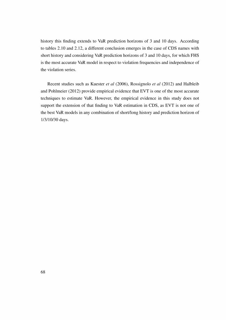
history this finding extends to VaR prediction horizons of 3 and 10 days. According
to tables 2.10 and 2.12, a different conclusion emerges in the case of CDS names with
short history and considering VaR prediction horizons of 3 and 10 days, for which FHS
is the most accurate VaR model in respect to violation frequencies and independence of
the violation series.
Recent studies such as Kuester et al (2006), Rossignolo et al (2012) and Halbleib
and Pohlmeier (2012) provide empirical evidence that EVT is one of the most accurate
techniques to estimate VaR. However, the empirical evidence in this study does not
support the extension of that finding to VaR estimation in CDS, as EVT is not one of
the best VaR models in any combination of short/long history and prediction horizon of
1/3/10/30 days.
68
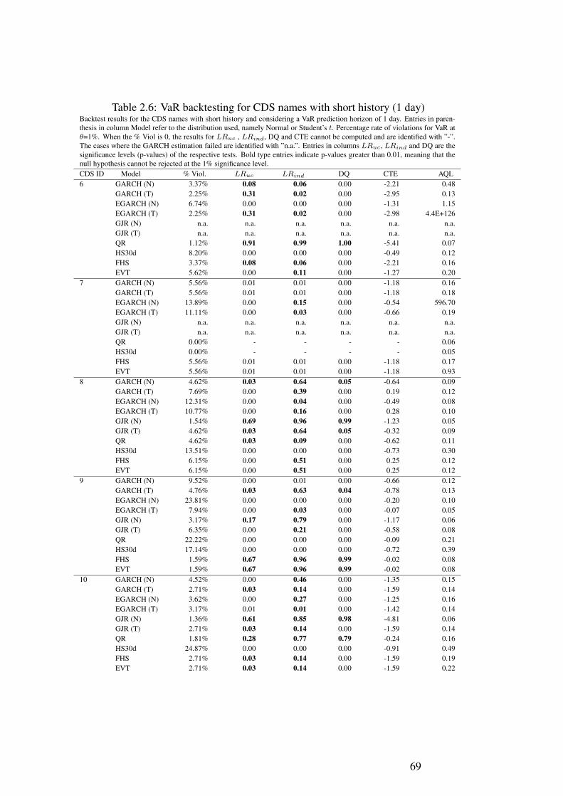
Table 2.6: VaR backtesting for CDS names with short history (1 day)Backtest results for the CDS names with short history and considering a VaR prediction horizon of 1 day. Entries in paren-thesis in column Model refer to the distribution used, namely Normal or Student’s t. Percentage rate of violations for VaR atθ=1%. When the % Viol is 0, the results for LRuc , LRind, DQ and CTE cannot be computed and are identified with ”-”.The cases where the GARCH estimation failed are identified with ”n.a.”. Entries in columns LRuc, LRind and DQ are thesignificance levels (p-values) of the respective tests. Bold type entries indicate p-values greater than 0.01, meaning that thenull hypothesis cannot be rejected at the 1% significance level.CDS ID Model % Viol. LRuc LRind DQ CTE AQL6 GARCH (N) 3.37% 0.08 0.06 0.00 -2.21 0.48
GARCH (T) 2.25% 0.31 0.02 0.00 -2.95 0.13EGARCH (N) 6.74% 0.00 0.00 0.00 -1.31 1.15EGARCH (T) 2.25% 0.31 0.02 0.00 -2.98 4.4E+126GJR (N) n.a. n.a. n.a. n.a. n.a. n.a.GJR (T) n.a. n.a. n.a. n.a. n.a. n.a.QR 1.12% 0.91 0.99 1.00 -5.41 0.07HS30d 8.20% 0.00 0.00 0.00 -0.49 0.12FHS 3.37% 0.08 0.06 0.00 -2.21 0.16EVT 5.62% 0.00 0.11 0.00 -1.27 0.20
7 GARCH (N) 5.56% 0.01 0.01 0.00 -1.18 0.16GARCH (T) 5.56% 0.01 0.01 0.00 -1.18 0.18EGARCH (N) 13.89% 0.00 0.15 0.00 -0.54 596.70EGARCH (T) 11.11% 0.00 0.03 0.00 -0.66 0.19GJR (N) n.a. n.a. n.a. n.a. n.a. n.a.GJR (T) n.a. n.a. n.a. n.a. n.a. n.a.QR 0.00% - - - - 0.06HS30d 0.00% - - - - 0.05FHS 5.56% 0.01 0.01 0.00 -1.18 0.17EVT 5.56% 0.01 0.01 0.00 -1.18 0.93
8 GARCH (N) 4.62% 0.03 0.64 0.05 -0.64 0.09GARCH (T) 7.69% 0.00 0.39 0.00 0.19 0.12EGARCH (N) 12.31% 0.00 0.04 0.00 -0.49 0.08EGARCH (T) 10.77% 0.00 0.16 0.00 0.28 0.10GJR (N) 1.54% 0.69 0.96 0.99 -1.23 0.05GJR (T) 4.62% 0.03 0.64 0.05 -0.32 0.09QR 4.62% 0.03 0.09 0.00 -0.62 0.11HS30d 13.51% 0.00 0.00 0.00 -0.73 0.30FHS 6.15% 0.00 0.51 0.00 0.25 0.12EVT 6.15% 0.00 0.51 0.00 0.25 0.12
9 GARCH (N) 9.52% 0.00 0.01 0.00 -0.66 0.12GARCH (T) 4.76% 0.03 0.63 0.04 -0.78 0.13EGARCH (N) 23.81% 0.00 0.00 0.00 -0.20 0.10EGARCH (T) 7.94% 0.00 0.03 0.00 -0.07 0.05GJR (N) 3.17% 0.17 0.79 0.00 -1.17 0.06GJR (T) 6.35% 0.00 0.21 0.00 -0.58 0.08QR 22.22% 0.00 0.00 0.00 -0.09 0.21HS30d 17.14% 0.00 0.00 0.00 -0.72 0.39FHS 1.59% 0.67 0.96 0.99 -0.02 0.08EVT 1.59% 0.67 0.96 0.99 -0.02 0.08
10 GARCH (N) 4.52% 0.00 0.46 0.00 -1.35 0.15GARCH (T) 2.71% 0.03 0.14 0.00 -1.59 0.14EGARCH (N) 3.62% 0.00 0.27 0.00 -1.25 0.16EGARCH (T) 3.17% 0.01 0.01 0.00 -1.42 0.14GJR (N) 1.36% 0.61 0.85 0.98 -4.81 0.06GJR (T) 2.71% 0.03 0.14 0.00 -1.59 0.14QR 1.81% 0.28 0.77 0.79 -0.24 0.16HS30d 24.87% 0.00 0.00 0.00 -0.91 0.49FHS 2.71% 0.03 0.14 0.00 -1.59 0.19EVT 2.71% 0.03 0.14 0.00 -1.59 0.22
69
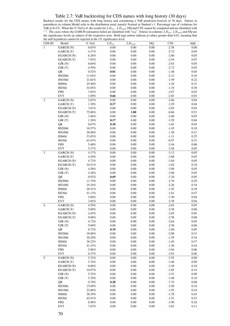
Table 2.7: VaR backtesting for CDS names with long history (30 days)Backtest results for the CDS names with long history and considering a VaR prediction horizon of 30 days. Entries inparenthesis in column Model refer to the distribution used, namely Normal or Student’s t. Percentage rate of violations forVaR at θ=1%. When the % Viol is 0, the results for LRuc , LRind, DQ and CTE cannot be computed and are identified with”-”. The cases where the GARCH estimation failed are identified with ”n.a.”. Entries in columns LRuc, LRind and DQ arethe significance levels (p-values) of the respective tests. Bold type entries indicate p-values greater than 0.01, meaning thatthe null hypothesis cannot be rejected at the 1% significance level.CDS ID Model % Viol. LRuc LRind DQ CTE AQL1 GARCH (N) 6.65% 0.00 0.00 0.00 -2.58 0.06
GARCH (T) 4.37% 0.00 0.00 0.00 -2.72 0.04EGARCH (N) 6.26% 0.00 0.00 0.00 -2.60 0.05EGARCH (T) 7.92% 0.00 0.00 0.00 -2.54 0.07GJR (N) 6.04% 0.00 0.00 0.00 -2.63 0.05GJR (T) 4.59% 0.00 0.00 0.00 -2.72 0.05QR 0.52% 0.01 0.00 0.00 -1.48 0.05HS200d 11.64% 0.00 0.00 0.00 -2.12 0.16HS100d 21.02% 0.00 0.00 0.00 -1.59 0.22HS60d 25.40% 0.00 0.00 0.00 -1.54 0.31HS30d 34.85% 0.00 0.00 0.00 -1.34 0.38FHS 3.02% 0.00 0.00 0.00 -2.67 0.03EVT 1.09% 0.66 0.00 0.00 -2.83 0.03
2 GARCH (N) 2.83% 0.00 0.00 0.00 -2.66 0.04GARCH (T) 1.30% 0.17 0.00 0.00 -3.29 0.04EGARCH (N) 3.01% 0.00 0.00 0.00 -2.65 0.05EGARCH (T) 75.88% 0.00 1.00 0.00 -0.66 0.51GJR (N) 3.46% 0.00 0.00 0.00 -2.60 0.05GJR (T) 1.30% 0.17 0.00 0.00 -3.29 0.04QR 0.67% 0.10 0.00 0.00 -1.65 0.05HS200d 16.57% 0.00 0.00 0.00 -1.45 0.18HS100d 26.08% 0.00 0.00 0.00 -1.20 0.21HS60d 33.03% 0.00 0.00 0.00 -1.11 0.25HS30d 41.67% 0.00 0.00 0.00 -0.97 0.31FHS 5.48% 0.00 0.00 0.00 -2.44 0.06EVT 5.17% 0.00 0.00 0.00 -2.48 0.05
3 GARCH (N) 4.17% 0.00 0.00 0.00 -3.13 0.05GARCH (T) 4.26% 0.00 0.00 0.00 -3.08 0.05EGARCH (N) 4.72% 0.00 0.00 0.00 -3.04 0.05EGARCH (T) 34.51% 0.00 0.00 0.00 -1.82 0.34GJR (N) 4.58% 0.00 0.00 0.00 -3.09 0.05GJR (T) 4.26% 0.00 0.00 0.00 -3.08 0.05QR 0.92% 0.69 0.00 0.00 -3.30 0.05HS200d 11.74% 0.00 0.00 0.00 -2.76 0.29HS100d 19.34% 0.00 0.00 0.00 -2.26 0.34HS60d 26.41% 0.00 0.00 0.00 -1.92 0.38HS30d 41.13% 0.00 0.00 0.00 -1.61 0.47FHS 2.66% 0.00 0.00 0.00 -3.30 0.04EVT 3.02% 0.00 0.00 0.00 -3.39 0.04
4 GARCH (N) 4.59% 0.00 0.00 0.00 -2.65 0.05GARCH (T) 5.69% 0.00 0.00 0.00 -2.58 0.06EGARCH (N) 4.45% 0.00 0.00 0.00 -2.65 0.05EGARCH (T) 9.08% 0.00 0.00 0.00 -2.58 0.08GJR (N) 4.72% 0.00 0.00 0.00 -2.64 0.05GJR (T) 5.69% 0.00 0.00 0.00 -2.58 0.06QR 0.73% 0.19 0.00 0.00 -2.60 0.05HS200d 18.86% 0.00 0.00 0.00 -2.08 0.31HS100d 30.20% 0.00 0.00 0.00 -1.59 0.34HS60d 36.22% 0.00 0.00 0.00 -1.45 0.37HS30d 41.43% 0.00 0.00 0.00 -1.36 0.44FHS 5.96% 0.00 0.00 0.00 -3.04 0.06EVT 6.37% 0.00 0.00 0.00 -3.03 0.06
5 GARCH (N) 5.32% 0.00 0.00 0.00 -3.55 0.09GARCH (T) 5.74% 0.00 0.00 0.00 -3.46 0.09EGARCH (N) 6.06% 0.00 0.00 0.00 -3.38 0.10EGARCH (T) 10.97% 0.00 0.00 0.00 -2.85 0.14GJR (N) 5.55% 0.00 0.00 0.00 -3.53 0.09GJR (T) 5.78% 0.00 0.00 0.00 -3.46 0.10QR 0.78% 0.28 0.00 0.00 -7.35 0.06HS200d 15.09% 0.00 0.00 0.00 -2.50 0.34HS100d 22.06% 0.00 0.00 0.00 -1.93 0.34HS60d 28.29% 0.00 0.00 0.00 -1.78 0.43HS30d 42.91% 0.00 0.00 0.00 -1.51 0.53FHS 6.98% 0.00 0.00 0.00 -3.90 0.10EVT 7.07% 0.00 0.00 0.00 -3.83 0.11
70
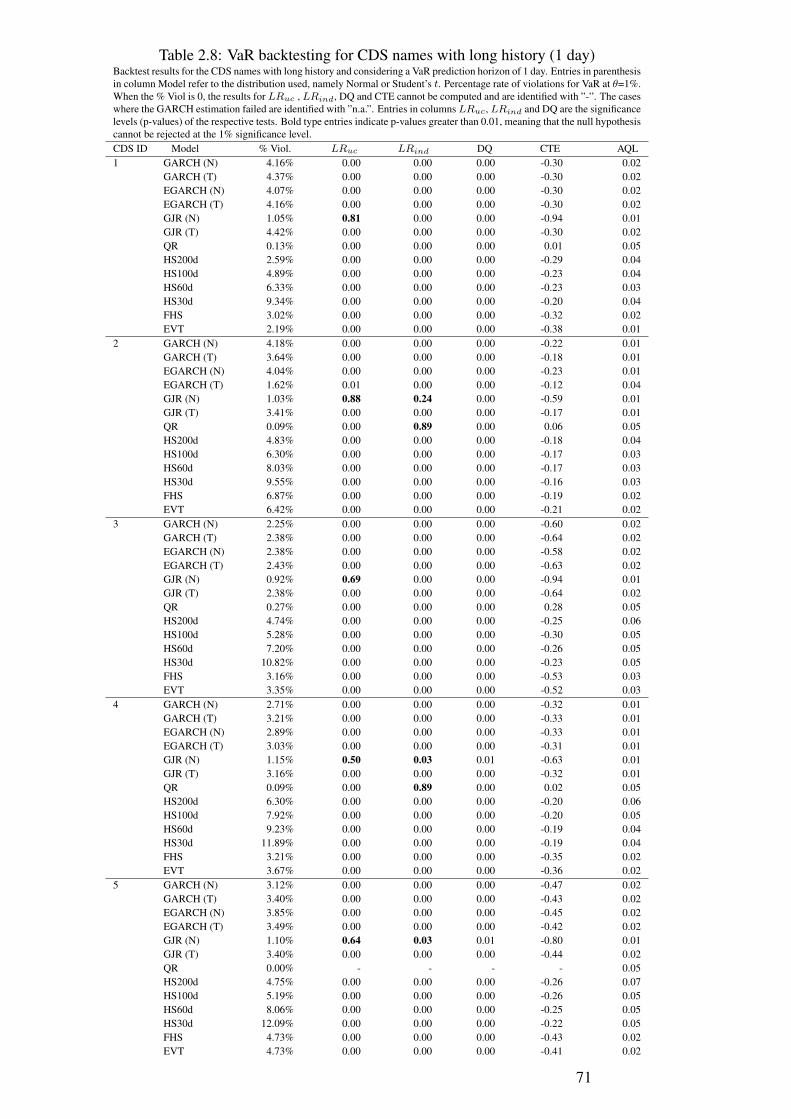
Table 2.8: VaR backtesting for CDS names with long history (1 day)Backtest results for the CDS names with long history and considering a VaR prediction horizon of 1 day. Entries in parenthesisin column Model refer to the distribution used, namely Normal or Student’s t. Percentage rate of violations for VaR at θ=1%.When the % Viol is 0, the results for LRuc , LRind, DQ and CTE cannot be computed and are identified with ”-”. The caseswhere the GARCH estimation failed are identified with ”n.a.”. Entries in columns LRuc, LRind and DQ are the significancelevels (p-values) of the respective tests. Bold type entries indicate p-values greater than 0.01, meaning that the null hypothesiscannot be rejected at the 1% significance level.CDS ID Model % Viol. LRuc LRind DQ CTE AQL1 GARCH (N) 4.16% 0.00 0.00 0.00 -0.30 0.02
GARCH (T) 4.37% 0.00 0.00 0.00 -0.30 0.02EGARCH (N) 4.07% 0.00 0.00 0.00 -0.30 0.02EGARCH (T) 4.16% 0.00 0.00 0.00 -0.30 0.02GJR (N) 1.05% 0.81 0.00 0.00 -0.94 0.01GJR (T) 4.42% 0.00 0.00 0.00 -0.30 0.02QR 0.13% 0.00 0.00 0.00 0.01 0.05HS200d 2.59% 0.00 0.00 0.00 -0.29 0.04HS100d 4.89% 0.00 0.00 0.00 -0.23 0.04HS60d 6.33% 0.00 0.00 0.00 -0.23 0.03HS30d 9.34% 0.00 0.00 0.00 -0.20 0.04FHS 3.02% 0.00 0.00 0.00 -0.32 0.02EVT 2.19% 0.00 0.00 0.00 -0.38 0.01
2 GARCH (N) 4.18% 0.00 0.00 0.00 -0.22 0.01GARCH (T) 3.64% 0.00 0.00 0.00 -0.18 0.01EGARCH (N) 4.04% 0.00 0.00 0.00 -0.23 0.01EGARCH (T) 1.62% 0.01 0.00 0.00 -0.12 0.04GJR (N) 1.03% 0.88 0.24 0.00 -0.59 0.01GJR (T) 3.41% 0.00 0.00 0.00 -0.17 0.01QR 0.09% 0.00 0.89 0.00 0.06 0.05HS200d 4.83% 0.00 0.00 0.00 -0.18 0.04HS100d 6.30% 0.00 0.00 0.00 -0.17 0.03HS60d 8.03% 0.00 0.00 0.00 -0.17 0.03HS30d 9.55% 0.00 0.00 0.00 -0.16 0.03FHS 6.87% 0.00 0.00 0.00 -0.19 0.02EVT 6.42% 0.00 0.00 0.00 -0.21 0.02
3 GARCH (N) 2.25% 0.00 0.00 0.00 -0.60 0.02GARCH (T) 2.38% 0.00 0.00 0.00 -0.64 0.02EGARCH (N) 2.38% 0.00 0.00 0.00 -0.58 0.02EGARCH (T) 2.43% 0.00 0.00 0.00 -0.63 0.02GJR (N) 0.92% 0.69 0.00 0.00 -0.94 0.01GJR (T) 2.38% 0.00 0.00 0.00 -0.64 0.02QR 0.27% 0.00 0.00 0.00 0.28 0.05HS200d 4.74% 0.00 0.00 0.00 -0.25 0.06HS100d 5.28% 0.00 0.00 0.00 -0.30 0.05HS60d 7.20% 0.00 0.00 0.00 -0.26 0.05HS30d 10.82% 0.00 0.00 0.00 -0.23 0.05FHS 3.16% 0.00 0.00 0.00 -0.53 0.03EVT 3.35% 0.00 0.00 0.00 -0.52 0.03
4 GARCH (N) 2.71% 0.00 0.00 0.00 -0.32 0.01GARCH (T) 3.21% 0.00 0.00 0.00 -0.33 0.01EGARCH (N) 2.89% 0.00 0.00 0.00 -0.33 0.01EGARCH (T) 3.03% 0.00 0.00 0.00 -0.31 0.01GJR (N) 1.15% 0.50 0.03 0.01 -0.63 0.01GJR (T) 3.16% 0.00 0.00 0.00 -0.32 0.01QR 0.09% 0.00 0.89 0.00 0.02 0.05HS200d 6.30% 0.00 0.00 0.00 -0.20 0.06HS100d 7.92% 0.00 0.00 0.00 -0.20 0.05HS60d 9.23% 0.00 0.00 0.00 -0.19 0.04HS30d 11.89% 0.00 0.00 0.00 -0.19 0.04FHS 3.21% 0.00 0.00 0.00 -0.35 0.02EVT 3.67% 0.00 0.00 0.00 -0.36 0.02
5 GARCH (N) 3.12% 0.00 0.00 0.00 -0.47 0.02GARCH (T) 3.40% 0.00 0.00 0.00 -0.43 0.02EGARCH (N) 3.85% 0.00 0.00 0.00 -0.45 0.02EGARCH (T) 3.49% 0.00 0.00 0.00 -0.42 0.02GJR (N) 1.10% 0.64 0.03 0.01 -0.80 0.01GJR (T) 3.40% 0.00 0.00 0.00 -0.44 0.02QR 0.00% - - - - 0.05HS200d 4.75% 0.00 0.00 0.00 -0.26 0.07HS100d 5.19% 0.00 0.00 0.00 -0.26 0.05HS60d 8.06% 0.00 0.00 0.00 -0.25 0.05HS30d 12.09% 0.00 0.00 0.00 -0.22 0.05FHS 4.73% 0.00 0.00 0.00 -0.43 0.02EVT 4.73% 0.00 0.00 0.00 -0.41 0.02
71
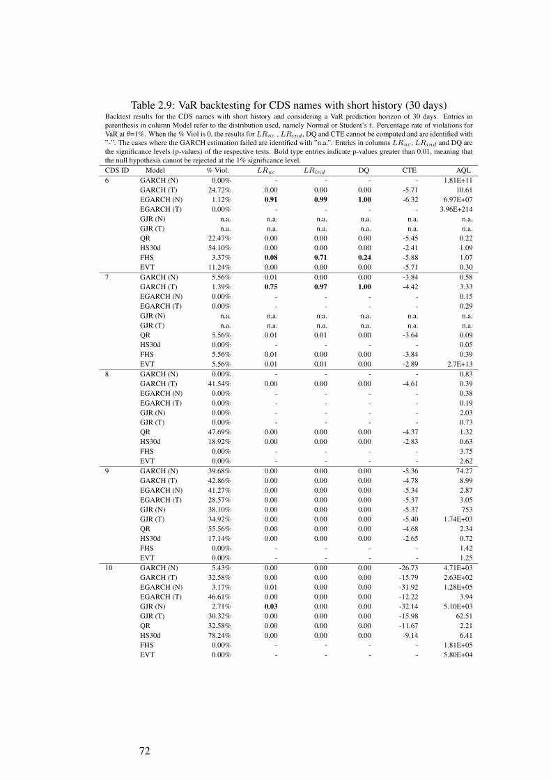
Table 2.9: VaR backtesting for CDS names with short history (30 days)Backtest results for the CDS names with short history and considering a VaR prediction horizon of 30 days. Entries inparenthesis in column Model refer to the distribution used, namely Normal or Student’s t. Percentage rate of violations forVaR at θ=1%. When the % Viol is 0, the results for LRuc , LRind, DQ and CTE cannot be computed and are identified with”-”. The cases where the GARCH estimation failed are identified with ”n.a.”. Entries in columns LRuc, LRind and DQ arethe significance levels (p-values) of the respective tests. Bold type entries indicate p-values greater than 0.01, meaning thatthe null hypothesis cannot be rejected at the 1% significance level.CDS ID Model % Viol. LRuc LRind DQ CTE AQL6 GARCH (N) 0.00% - - - - 1.81E+11
GARCH (T) 24.72% 0.00 0.00 0.00 -5.71 10.61EGARCH (N) 1.12% 0.91 0.99 1.00 -6.32 6.97E+07EGARCH (T) 0.00% - - - - 3.96E+214GJR (N) n.a. n.a. n.a. n.a. n.a. n.a.GJR (T) n.a. n.a. n.a. n.a. n.a. n.a.QR 22.47% 0.00 0.00 0.00 -5.45 0.22HS30d 54.10% 0.00 0.00 0.00 -2.41 1.09FHS 3.37% 0.08 0.71 0.24 -5.88 1.07EVT 11.24% 0.00 0.00 0.00 -5.71 0.30
7 GARCH (N) 5.56% 0.01 0.00 0.00 -3.84 0.58GARCH (T) 1.39% 0.75 0.97 1.00 -4.42 3.33EGARCH (N) 0.00% - - - - 0.15EGARCH (T) 0.00% - - - - 0.29GJR (N) n.a. n.a. n.a. n.a. n.a. n.a.GJR (T) n.a. n.a. n.a. n.a. n.a. n.a.QR 5.56% 0.01 0.01 0.00 -3.64 0.09HS30d 0.00% - - - - 0.05FHS 5.56% 0.01 0.00 0.00 -3.84 0.39EVT 5.56% 0.01 0.01 0.00 -2.89 2.7E+13
8 GARCH (N) 0.00% - - - - 0.83GARCH (T) 41.54% 0.00 0.00 0.00 -4.61 0.39EGARCH (N) 0.00% - - - - 0.38EGARCH (T) 0.00% - - - - 0.19GJR (N) 0.00% - - - - 2.03GJR (T) 0.00% - - - - 0.73QR 47.69% 0.00 0.00 0.00 -4.37 1.32HS30d 18.92% 0.00 0.00 0.00 -2.83 0.63FHS 0.00% - - - - 3.75EVT 0.00% - - - - 2.62
9 GARCH (N) 39.68% 0.00 0.00 0.00 -5.36 74.27GARCH (T) 42.86% 0.00 0.00 0.00 -4.78 8.99EGARCH (N) 41.27% 0.00 0.00 0.00 -5.34 2.87EGARCH (T) 28.57% 0.00 0.00 0.00 -5.37 3.05GJR (N) 38.10% 0.00 0.00 0.00 -5.37 753GJR (T) 34.92% 0.00 0.00 0.00 -5.40 1.74E+03QR 55.56% 0.00 0.00 0.00 -4.68 2.34HS30d 17.14% 0.00 0.00 0.00 -2.65 0.72FHS 0.00% - - - - 1.42EVT 0.00% - - - - 1.25
10 GARCH (N) 5.43% 0.00 0.00 0.00 -26.73 4.71E+03GARCH (T) 32.58% 0.00 0.00 0.00 -15.79 2.63E+02EGARCH (N) 3.17% 0.01 0.00 0.00 -31.92 1.28E+05EGARCH (T) 46.61% 0.00 0.00 0.00 -12.22 3.94GJR (N) 2.71% 0.03 0.00 0.00 -32.14 5.10E+03GJR (T) 30.32% 0.00 0.00 0.00 -15.98 62.51QR 32.58% 0.00 0.00 0.00 -11.67 2.21HS30d 78.24% 0.00 0.00 0.00 -9.14 6.41FHS 0.00% - - - - 1.81E+05EVT 0.00% - - - - 5.80E+04
72
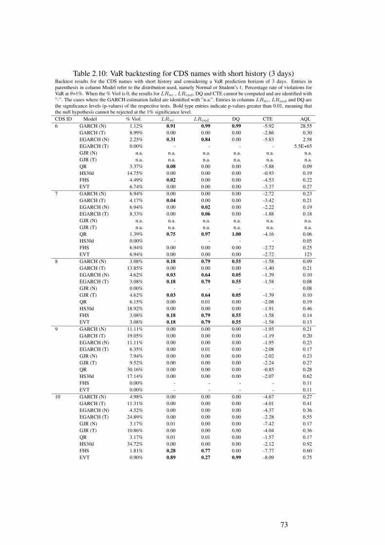
Table 2.10: VaR backtesting for CDS names with short history (3 days)Backtest results for the CDS names with short history and considering a VaR prediction horizon of 3 days. Entries inparenthesis in column Model refer to the distribution used, namely Normal or Student’s t. Percentage rate of violations forVaR at θ=1%. When the % Viol is 0, the results for LRuc , LRind, DQ and CTE cannot be computed and are identified with”-”. The cases where the GARCH estimation failed are identified with ”n.a.”. Entries in columns LRuc, LRind and DQ arethe significance levels (p-values) of the respective tests. Bold type entries indicate p-values greater than 0.01, meaning thatthe null hypothesis cannot be rejected at the 1% significance level.CDS ID Model % Viol. LRuc LRind DQ CTE AQL6 GARCH (N) 1.12% 0.91 0.99 0.99 -5.92 28.55
GARCH (T) 8.99% 0.00 0.00 0.00 -2.86 0.30EGARCH (N) 2.25% 0.31 0.84 0.00 -5.83 2.58EGARCH (T) 0.00% - - - - 5.5E+65GJR (N) n.a. n.a. n.a. n.a. n.a. n.a.GJR (T) n.a. n.a. n.a. n.a. n.a. n.a.QR 3.37% 0.08 0.00 0.00 -5.88 0.09HS30d 14.75% 0.00 0.00 0.00 -0.93 0.19FHS 4.49% 0.02 0.00 0.00 -4.53 0.22EVT 6.74% 0.00 0.00 0.00 -3.37 0.27
7 GARCH (N) 6.94% 0.00 0.00 0.00 -2.72 0.23GARCH (T) 4.17% 0.04 0.00 0.00 -3.42 0.21EGARCH (N) 6.94% 0.00 0.02 0.00 -2.22 0.19EGARCH (T) 8.33% 0.00 0.06 0.00 -1.88 0.18GJR (N) n.a. n.a. n.a. n.a. n.a. n.a.GJR (T) n.a. n.a. n.a. n.a. n.a. n.a.QR 1.39% 0.75 0.97 1.00 -4.16 0.06HS30d 0.00% - - - - 0.05FHS 6.94% 0.00 0.00 0.00 -2.72 0.25EVT 6.94% 0.00 0.00 0.00 -2.72 123
8 GARCH (N) 3.08% 0.18 0.79 0.55 -1.58 0.09GARCH (T) 13.85% 0.00 0.00 0.00 -1.40 0.21EGARCH (N) 4.62% 0.03 0.64 0.05 -1.39 0.10EGARCH (T) 3.08% 0.18 0.79 0.55 -1.58 0.08GJR (N) 0.00% - - - - 0.08GJR (T) 4.62% 0.03 0.64 0.05 -1.39 0.10QR 6.15% 0.00 0.01 0.00 -2.08 0.19HS30d 18.92% 0.00 0.00 0.00 -1.91 0.46FHS 3.08% 0.18 0.79 0.55 -1.58 0.14EVT 3.08% 0.18 0.79 0.55 -1.58 0.13
9 GARCH (N) 11.11% 0.00 0.00 0.00 -1.95 0.21GARCH (T) 19.05% 0.00 0.00 0.00 -1.19 0.20EGARCH (N) 11.11% 0.00 0.00 0.00 -1.95 0.23EGARCH (T) 6.35% 0.00 0.01 0.00 -2.08 0.17GJR (N) 7.94% 0.00 0.00 0.00 -2.02 0.23GJR (T) 9.52% 0.00 0.00 0.00 -2.24 0.27QR 30.16% 0.00 0.00 0.00 -0.85 0.28HS30d 17.14% 0.00 0.00 0.00 -2.07 0.62FHS 0.00% - - - - 0.11EVT 0.00% - - - - 0.11
10 GARCH (N) 4.98% 0.00 0.00 0.00 -4.67 0.27GARCH (T) 11.31% 0.00 0.00 0.00 -4.01 0.41EGARCH (N) 4.52% 0.00 0.00 0.00 -4.37 0.36EGARCH (T) 24.89% 0.00 0.00 0.00 -2.28 0.55GJR (N) 3.17% 0.01 0.00 0.00 -7.42 0.17GJR (T) 10.86% 0.00 0.00 0.00 -4.04 0.36QR 3.17% 0.01 0.01 0.00 -1.57 0.17HS30d 34.72% 0.00 0.00 0.00 -2.12 0.92FHS 1.81% 0.28 0.77 0.00 -7.77 0.60EVT 0.90% 0.89 0.27 0.99 -8.09 0.75
73
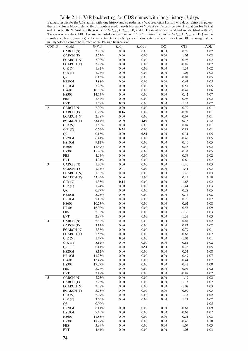
Table 2.11: VaR backtesting for CDS names with long history (3 days)Backtest results for the CDS names with long history and considering a VaR prediction horizon of 3 days. Entries in paren-thesis in column Model refer to the distribution used, namely Normal or Student’s t. Percentage rate of violations for VaR atθ=1%. When the % Viol is 0, the results for LRuc , LRind, DQ and CTE cannot be computed and are identified with ”-”.The cases where the GARCH estimation failed are identified with ”n.a.”. Entries in columns LRuc, LRind and DQ are thesignificance levels (p-values) of the respective tests. Bold type entries indicate p-values greater than 0.01, meaning that thenull hypothesis cannot be rejected at the 1% significance level.CDS ID Model % Viol. LRuc LRind DQ CTE AQL1 GARCH (N) 3.28% 0.00 0.00 0.00 -0.95 0.02
GARCH (T) 2.27% 0.00 0.00 0.00 -1.02 0.02EGARCH (N) 3.02% 0.00 0.00 0.00 -0.98 0.02EGARCH (T) 3.98% 0.00 0.00 0.00 -0.89 0.02GJR (N) 1.92% 0.00 0.00 0.00 -1.33 0.02GJR (T) 2.27% 0.00 0.00 0.00 -1.02 0.02QR 0.13% 0.00 0.00 0.00 -0.01 0.05HS200d 3.88% 0.00 0.00 0.00 -0.64 0.05HS100d 7.22% 0.00 0.00 0.00 -0.51 0.05HS60d 10.05% 0.00 0.00 0.00 -0.48 0.06HS30d 14.53% 0.00 0.00 0.00 -0.42 0.07FHS 2.32% 0.00 0.00 0.00 -0.98 0.02EVT 1.49% 0.03 0.00 0.00 -1.12 0.02
2 GARCH (N) 2.20% 0.00 0.00 0.00 -0.70 0.01GARCH (T) 0.72% 0.16 0.00 0.00 -0.91 0.01EGARCH (N) 2.38% 0.00 0.00 0.00 -0.67 0.01EGARCH (T) 55.12% 0.00 1.00 0.00 -0.17 0.15GJR (N) 1.66% 0.00 0.00 0.00 -0.89 0.01GJR (T) 0.76% 0.24 0.00 0.00 -0.88 0.01QR 0.13% 0.00 0.94 0.00 -0.34 0.05HS200d 6.41% 0.00 0.00 0.00 -0.45 0.05HS100d 9.12% 0.00 0.00 0.00 -0.40 0.05HS60d 12.59% 0.00 0.00 0.00 -0.36 0.05HS30d 15.20% 0.00 0.00 0.00 -0.33 0.05FHS 4.94% 0.00 0.00 0.00 -0.58 0.02EVT 4.94% 0.00 0.00 0.00 -0.60 0.02
3 GARCH (N) 1.70% 0.00 0.00 0.00 -1.46 0.03GARCH (T) 1.65% 0.01 0.00 0.00 -1.44 0.03EGARCH (N) 1.88% 0.00 0.00 0.00 -1.40 0.03EGARCH (T) 22.46% 0.00 1.00 0.00 -0.49 0.10GJR (N) 1.33% 0.14 0.00 0.00 -1.66 0.02GJR (T) 1.74% 0.00 0.00 0.00 -1.44 0.03QR 0.27% 0.00 0.00 0.00 0.28 0.05HS200d 5.75% 0.00 0.00 0.00 -0.71 0.08HS100d 7.15% 0.00 0.00 0.00 -0.76 0.07HS60d 10.73% 0.00 0.00 0.00 -0.62 0.08HS30d 16.02% 0.00 0.00 0.00 -0.53 0.09FHS 2.98% 0.00 0.00 0.00 -1.30 0.03EVT 2.89% 0.00 0.00 0.00 -1.31 0.03
4 GARCH (N) 2.66% 0.00 0.00 0.00 -0.81 0.02GARCH (T) 3.12% 0.00 0.00 0.00 -0.82 0.02EGARCH (N) 2.38% 0.00 0.00 0.00 -0.79 0.01EGARCH (T) 5.55% 0.00 0.00 0.00 -0.68 0.02GJR (N) 1.47% 0.04 0.00 0.00 -1.02 0.01GJR (T) 3.12% 0.00 0.00 0.00 -0.82 0.02QR 0.14% 0.00 0.94 0.00 -0.42 0.05HS200d 8.12% 0.00 0.00 0.00 -0.54 0.08HS100d 11.23% 0.00 0.00 0.00 -0.49 0.07HS60d 13.47% 0.00 0.00 0.00 -0.44 0.07HS30d 17.37% 0.00 0.00 0.00 -0.41 0.08FHS 3.76% 0.00 0.00 0.00 -0.91 0.02EVT 3.48% 0.00 0.00 0.00 -0.88 0.02
5 GARCH (N) 2.75% 0.00 0.00 0.00 -1.19 0.02GARCH (T) 3.26% 0.00 0.00 0.00 -1.13 0.02EGARCH (N) 3.58% 0.00 0.00 0.00 -1.08 0.03EGARCH (T) 5.78% 0.00 0.00 0.00 -0.90 0.03GJR (N) 2.29% 0.00 0.00 0.00 -1.33 0.02GJR (T) 3.26% 0.00 0.00 0.00 -1.13 0.02QR 0.00% - - - - 0.05HS200d 6.11% 0.00 0.00 0.00 -0.67 0.09HS100d 7.45% 0.00 0.00 0.00 -0.61 0.07HS60d 11.83% 0.00 0.00 0.00 -0.54 0.08HS30d 18.27% 0.00 0.00 0.00 -0.46 0.10FHS 3.99% 0.00 0.00 0.00 -1.09 0.03EVT 4.64% 0.00 0.00 0.00 -1.05 0.03
74
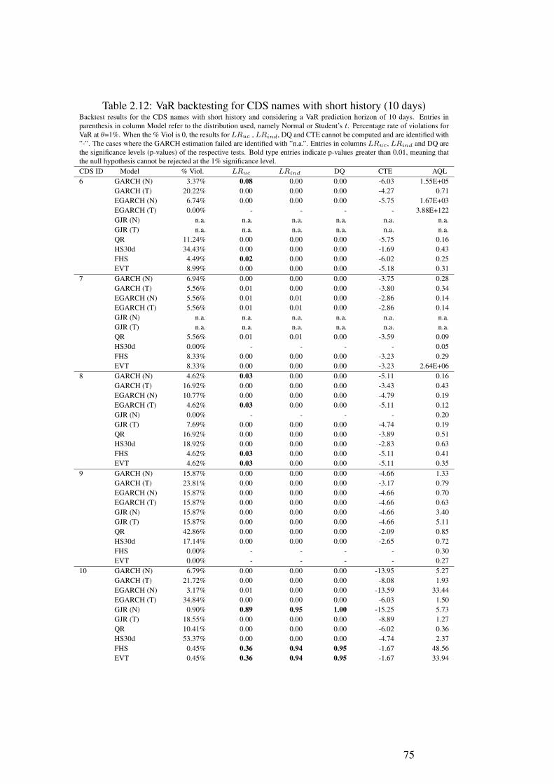
Table 2.12: VaR backtesting for CDS names with short history (10 days)Backtest results for the CDS names with short history and considering a VaR prediction horizon of 10 days. Entries inparenthesis in column Model refer to the distribution used, namely Normal or Student’s t. Percentage rate of violations forVaR at θ=1%. When the % Viol is 0, the results for LRuc , LRind, DQ and CTE cannot be computed and are identified with”-”. The cases where the GARCH estimation failed are identified with ”n.a.”. Entries in columns LRuc, LRind and DQ arethe significance levels (p-values) of the respective tests. Bold type entries indicate p-values greater than 0.01, meaning thatthe null hypothesis cannot be rejected at the 1% significance level.CDS ID Model % Viol. LRuc LRind DQ CTE AQL6 GARCH (N) 3.37% 0.08 0.00 0.00 -6.03 1.55E+05
GARCH (T) 20.22% 0.00 0.00 0.00 -4.27 0.71EGARCH (N) 6.74% 0.00 0.00 0.00 -5.75 1.67E+03EGARCH (T) 0.00% - - - - 3.88E+122GJR (N) n.a. n.a. n.a. n.a. n.a. n.a.GJR (T) n.a. n.a. n.a. n.a. n.a. n.a.QR 11.24% 0.00 0.00 0.00 -5.75 0.16HS30d 34.43% 0.00 0.00 0.00 -1.69 0.43FHS 4.49% 0.02 0.00 0.00 -6.02 0.25EVT 8.99% 0.00 0.00 0.00 -5.18 0.31
7 GARCH (N) 6.94% 0.00 0.00 0.00 -3.75 0.28GARCH (T) 5.56% 0.01 0.00 0.00 -3.80 0.34EGARCH (N) 5.56% 0.01 0.01 0.00 -2.86 0.14EGARCH (T) 5.56% 0.01 0.01 0.00 -2.86 0.14GJR (N) n.a. n.a. n.a. n.a. n.a. n.a.GJR (T) n.a. n.a. n.a. n.a. n.a. n.a.QR 5.56% 0.01 0.01 0.00 -3.59 0.09HS30d 0.00% - - - - 0.05FHS 8.33% 0.00 0.00 0.00 -3.23 0.29EVT 8.33% 0.00 0.00 0.00 -3.23 2.64E+06
8 GARCH (N) 4.62% 0.03 0.00 0.00 -5.11 0.16GARCH (T) 16.92% 0.00 0.00 0.00 -3.43 0.43EGARCH (N) 10.77% 0.00 0.00 0.00 -4.79 0.19EGARCH (T) 4.62% 0.03 0.00 0.00 -5.11 0.12GJR (N) 0.00% - - - - 0.20GJR (T) 7.69% 0.00 0.00 0.00 -4.74 0.19QR 16.92% 0.00 0.00 0.00 -3.89 0.51HS30d 18.92% 0.00 0.00 0.00 -2.83 0.63FHS 4.62% 0.03 0.00 0.00 -5.11 0.41EVT 4.62% 0.03 0.00 0.00 -5.11 0.35
9 GARCH (N) 15.87% 0.00 0.00 0.00 -4.66 1.33GARCH (T) 23.81% 0.00 0.00 0.00 -3.17 0.79EGARCH (N) 15.87% 0.00 0.00 0.00 -4.66 0.70EGARCH (T) 15.87% 0.00 0.00 0.00 -4.66 0.63GJR (N) 15.87% 0.00 0.00 0.00 -4.66 3.40GJR (T) 15.87% 0.00 0.00 0.00 -4.66 5.11QR 42.86% 0.00 0.00 0.00 -2.09 0.85HS30d 17.14% 0.00 0.00 0.00 -2.65 0.72FHS 0.00% - - - - 0.30EVT 0.00% - - - - 0.27
10 GARCH (N) 6.79% 0.00 0.00 0.00 -13.95 5.27GARCH (T) 21.72% 0.00 0.00 0.00 -8.08 1.93EGARCH (N) 3.17% 0.01 0.00 0.00 -13.59 33.44EGARCH (T) 34.84% 0.00 0.00 0.00 -6.03 1.50GJR (N) 0.90% 0.89 0.95 1.00 -15.25 5.73GJR (T) 18.55% 0.00 0.00 0.00 -8.89 1.27QR 10.41% 0.00 0.00 0.00 -6.02 0.36HS30d 53.37% 0.00 0.00 0.00 -4.74 2.37FHS 0.45% 0.36 0.94 0.95 -1.67 48.56EVT 0.45% 0.36 0.94 0.95 -1.67 33.94
75
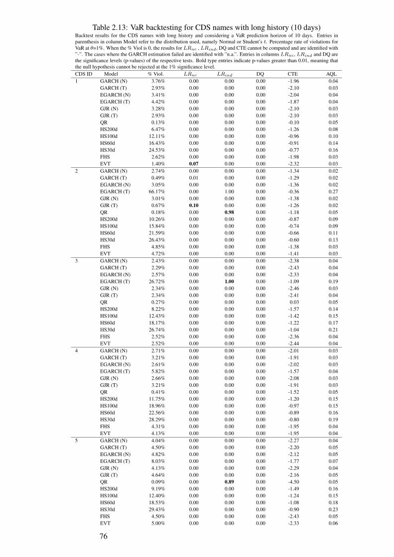
Table 2.13: VaR backtesting for CDS names with long history (10 days)Backtest results for the CDS names with long history and considering a VaR prediction horizon of 10 days. Entries inparenthesis in column Model refer to the distribution used, namely Normal or Student’s t. Percentage rate of violations forVaR at θ=1%. When the % Viol is 0, the results for LRuc , LRind, DQ and CTE cannot be computed and are identified with”-”. The cases where the GARCH estimation failed are identified with ”n.a.”. Entries in columns LRuc, LRind and DQ arethe significance levels (p-values) of the respective tests. Bold type entries indicate p-values greater than 0.01, meaning thatthe null hypothesis cannot be rejected at the 1% significance level.CDS ID Model % Viol. LRuc LRind DQ CTE AQL1 GARCH (N) 3.76% 0.00 0.00 0.00 -1.96 0.04
GARCH (T) 2.93% 0.00 0.00 0.00 -2.10 0.03EGARCH (N) 3.41% 0.00 0.00 0.00 -2.04 0.04EGARCH (T) 4.42% 0.00 0.00 0.00 -1.87 0.04GJR (N) 3.28% 0.00 0.00 0.00 -2.10 0.03GJR (T) 2.93% 0.00 0.00 0.00 -2.10 0.03QR 0.13% 0.00 0.00 0.00 -0.10 0.05HS200d 6.47% 0.00 0.00 0.00 -1.26 0.08HS100d 12.11% 0.00 0.00 0.00 -0.96 0.10HS60d 16.43% 0.00 0.00 0.00 -0.91 0.14HS30d 24.53% 0.00 0.00 0.00 -0.77 0.16FHS 2.62% 0.00 0.00 0.00 -1.98 0.03EVT 1.40% 0.07 0.00 0.00 -2.32 0.03
2 GARCH (N) 2.74% 0.00 0.00 0.00 -1.34 0.02GARCH (T) 0.49% 0.01 0.00 0.00 -1.29 0.02EGARCH (N) 3.05% 0.00 0.00 0.00 -1.36 0.02EGARCH (T) 66.17% 0.00 1.00 0.00 -0.36 0.27GJR (N) 3.01% 0.00 0.00 0.00 -1.38 0.02GJR (T) 0.67% 0.10 0.00 0.00 -1.26 0.02QR 0.18% 0.00 0.98 0.00 -1.18 0.05HS200d 10.26% 0.00 0.00 0.00 -0.87 0.09HS100d 15.84% 0.00 0.00 0.00 -0.74 0.09HS60d 21.59% 0.00 0.00 0.00 -0.66 0.11HS30d 26.43% 0.00 0.00 0.00 -0.60 0.13FHS 4.85% 0.00 0.00 0.00 -1.38 0.03EVT 4.72% 0.00 0.00 0.00 -1.41 0.03
3 GARCH (N) 2.43% 0.00 0.00 0.00 -2.38 0.04GARCH (T) 2.29% 0.00 0.00 0.00 -2.43 0.04EGARCH (N) 2.57% 0.00 0.00 0.00 -2.33 0.04EGARCH (T) 26.72% 0.00 1.00 0.00 -1.09 0.19GJR (N) 2.34% 0.00 0.00 0.00 -2.46 0.03GJR (T) 2.34% 0.00 0.00 0.00 -2.41 0.04QR 0.27% 0.00 0.00 0.00 0.03 0.05HS200d 8.22% 0.00 0.00 0.00 -1.57 0.14HS100d 12.43% 0.00 0.00 0.00 -1.42 0.15HS60d 18.17% 0.00 0.00 0.00 -1.22 0.17HS30d 26.74% 0.00 0.00 0.00 -1.04 0.21FHS 2.52% 0.00 0.00 0.00 -2.36 0.04EVT 2.52% 0.00 0.00 0.00 -2.44 0.04
4 GARCH (N) 2.71% 0.00 0.00 0.00 -2.01 0.03GARCH (T) 3.21% 0.00 0.00 0.00 -1.91 0.03EGARCH (N) 2.61% 0.00 0.00 0.00 -2.02 0.03EGARCH (T) 5.82% 0.00 0.00 0.00 -1.57 0.04GJR (N) 2.66% 0.00 0.00 0.00 -2.08 0.03GJR (T) 3.21% 0.00 0.00 0.00 -1.91 0.03QR 0.41% 0.00 0.00 0.00 -1.52 0.05HS200d 11.75% 0.00 0.00 0.00 -1.20 0.15HS100d 18.96% 0.00 0.00 0.00 -0.97 0.15HS60d 22.56% 0.00 0.00 0.00 -0.89 0.16HS30d 28.29% 0.00 0.00 0.00 -0.80 0.19FHS 4.31% 0.00 0.00 0.00 -1.95 0.04EVT 4.13% 0.00 0.00 0.00 -1.95 0.04
5 GARCH (N) 4.04% 0.00 0.00 0.00 -2.27 0.04GARCH (T) 4.50% 0.00 0.00 0.00 -2.20 0.05EGARCH (N) 4.82% 0.00 0.00 0.00 -2.12 0.05EGARCH (T) 8.03% 0.00 0.00 0.00 -1.77 0.07GJR (N) 4.13% 0.00 0.00 0.00 -2.29 0.04GJR (T) 4.64% 0.00 0.00 0.00 -2.16 0.05QR 0.09% 0.00 0.89 0.00 -4.50 0.05HS200d 9.19% 0.00 0.00 0.00 -1.49 0.16HS100d 12.40% 0.00 0.00 0.00 -1.24 0.15HS60d 18.53% 0.00 0.00 0.00 -1.08 0.18HS30d 29.43% 0.00 0.00 0.00 -0.90 0.23FHS 4.50% 0.00 0.00 0.00 -2.43 0.05EVT 5.00% 0.00 0.00 0.00 -2.33 0.06
76
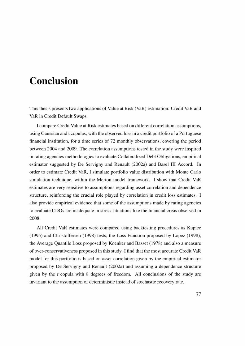
Conclusion
This thesis presents two applications of Value at Risk (VaR) estimation: Credit VaR and
VaR in Credit Default Swaps.
I compare Credit Value at Risk estimates based on different correlation assumptions,
using Gaussian and t copulas, with the observed loss in a credit portfolio of a Portuguese
financial institution, for a time series of 72 monthly observations, covering the period
between 2004 and 2009. The correlation assumptions tested in the study were inspired
in rating agencies methodologies to evaluate Collateralized Debt Obligations, empirical
estimator suggested by De Servigny and Renault (2002a) and Basel III Accord. In
order to estimate Credit VaR, I simulate portfolio value distribution with Monte Carlo
simulation technique, within the Merton model framework. I show that Credit VaR
estimates are very sensitive to assumptions regarding asset correlation and dependence
structure, reinforcing the crucial role played by correlation in credit loss estimates. I
also provide empirical evidence that some of the assumptions made by rating agencies
to evaluate CDOs are inadequate in stress situations like the financial crisis observed in
2008.
All Credit VaR estimates were compared using backtesting procedures as Kupiec
(1995) and Christoffersen (1998) tests, the Loss Function proposed by Lopez (1998),
the Average Quantile Loss proposed by Koenker and Basset (1978) and also a measure
of over-conservativeness proposed in this study. I find that the most accurate Credit VaR
model for this portfolio is based on asset correlation given by the empirical estimator
proposed by De Servigny and Renault (2002a) and assuming a dependence structure
given by the t copula with 8 degrees of freedom. All conclusions of the study are
invariant to the assumption of deterministic instead of stochastic recovery rate.
77
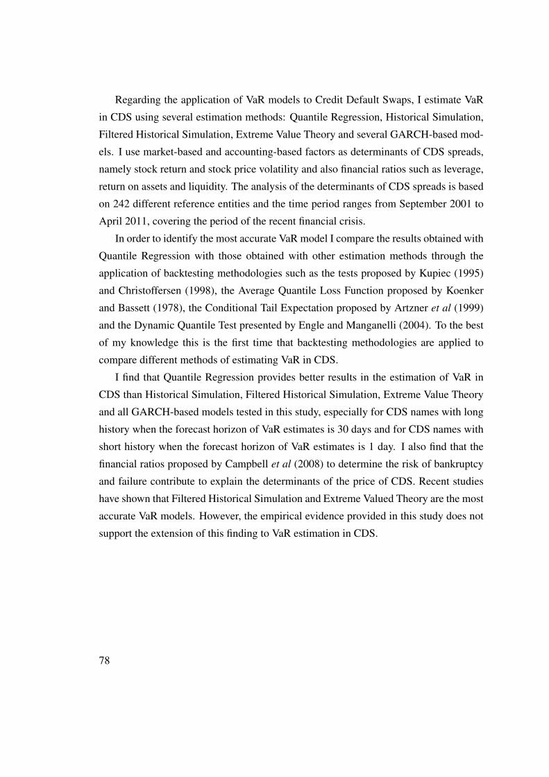
Regarding the application of VaR models to Credit Default Swaps, I estimate VaR
in CDS using several estimation methods: Quantile Regression, Historical Simulation,
Filtered Historical Simulation, Extreme Value Theory and several GARCH-based mod-
els. I use market-based and accounting-based factors as determinants of CDS spreads,
namely stock return and stock price volatility and also financial ratios such as leverage,
return on assets and liquidity. The analysis of the determinants of CDS spreads is based
on 242 different reference entities and the time period ranges from September 2001 to
April 2011, covering the period of the recent financial crisis.
In order to identify the most accurate VaR model I compare the results obtained with
Quantile Regression with those obtained with other estimation methods through the
application of backtesting methodologies such as the tests proposed by Kupiec (1995)
and Christoffersen (1998), the Average Quantile Loss Function proposed by Koenker
and Bassett (1978), the Conditional Tail Expectation proposed by Artzner et al (1999)
and the Dynamic Quantile Test presented by Engle and Manganelli (2004). To the best
of my knowledge this is the first time that backtesting methodologies are applied to
compare different methods of estimating VaR in CDS.
I find that Quantile Regression provides better results in the estimation of VaR in
CDS than Historical Simulation, Filtered Historical Simulation, Extreme Value Theory
and all GARCH-based models tested in this study, especially for CDS names with long
history when the forecast horizon of VaR estimates is 30 days and for CDS names with
short history when the forecast horizon of VaR estimates is 1 day. I also find that the
financial ratios proposed by Campbell et al (2008) to determine the risk of bankruptcy
and failure contribute to explain the determinants of the price of CDS. Recent studies
have shown that Filtered Historical Simulation and Extreme Valued Theory are the most
accurate VaR models. However, the empirical evidence provided in this study does not
support the extension of this finding to VaR estimation in CDS.
78

Appendix A
79

To simplify the analysis I assume that the default indicator Ii,t is exchangeable. A
random vector S is called exchangeable if
(S1, ...Sm)d= (SΠ(1), ..., SΠ(M))
for any permutation (Π(1), ...Π(m)) of (1, ...,m). The consequence is that for any
j ∈ 1, ...,m − 1 all of the(mj
)possible j-dimensional marginal distributions of S
are identical. In this situation, default probabilities and joint default probabilities are
given by
πj := P (Ii1 = 1, ..., Iij = 1), i1, ..., ij ⊂ 1, ...,m, 1 ≤ j ≤ m,
π := π1 = P (Ii = 1), i ∈ 1, ...,m
The jth order joint default probability, πj , is the probability that an arbitrarily se-
lected subgroup of j obligors defaults.
I will now introduce the definition of Bernoulli mixture model and explain under
which conditions this model is exchangeable. This setup is the mathematical base of the
joint default probability estimator. For this purpose, consider a generic exchangeable
group of N obligors where D obligors default.
Definition 1 (Bernoulli Mixture Model) Given some p < N and a p−dimensional
random vector Ψ = (Ψ1, ...,Ψp), the random vector I = (I1, ..., IN)′ follows a Bernoulli
mixture model with factor vector Ψ if there are functions Qi : Rp → [0, 1], 1 ≤ i ≤ N ,
such that conditional on Ψ the default indicator I is a vector of independent Bernoulli
random variables with P (Ii = 1|Ψ) = Qi(Ψ).
A Bernoulli mixture model is exchangeable if the functions Qi are all identical and,
in that case, the vector I is exchangeable. Considering the random variable Q := Q1(Ψ)
we get for I = (I1, ..., IN)′ in 0, 1N
P (I = I|Ψ) = Q1(Ψ)∑Ni=1 Ii(1−Q1(Ψ))N−
∑Ni=1 Ii = P (I = I|Q)
80
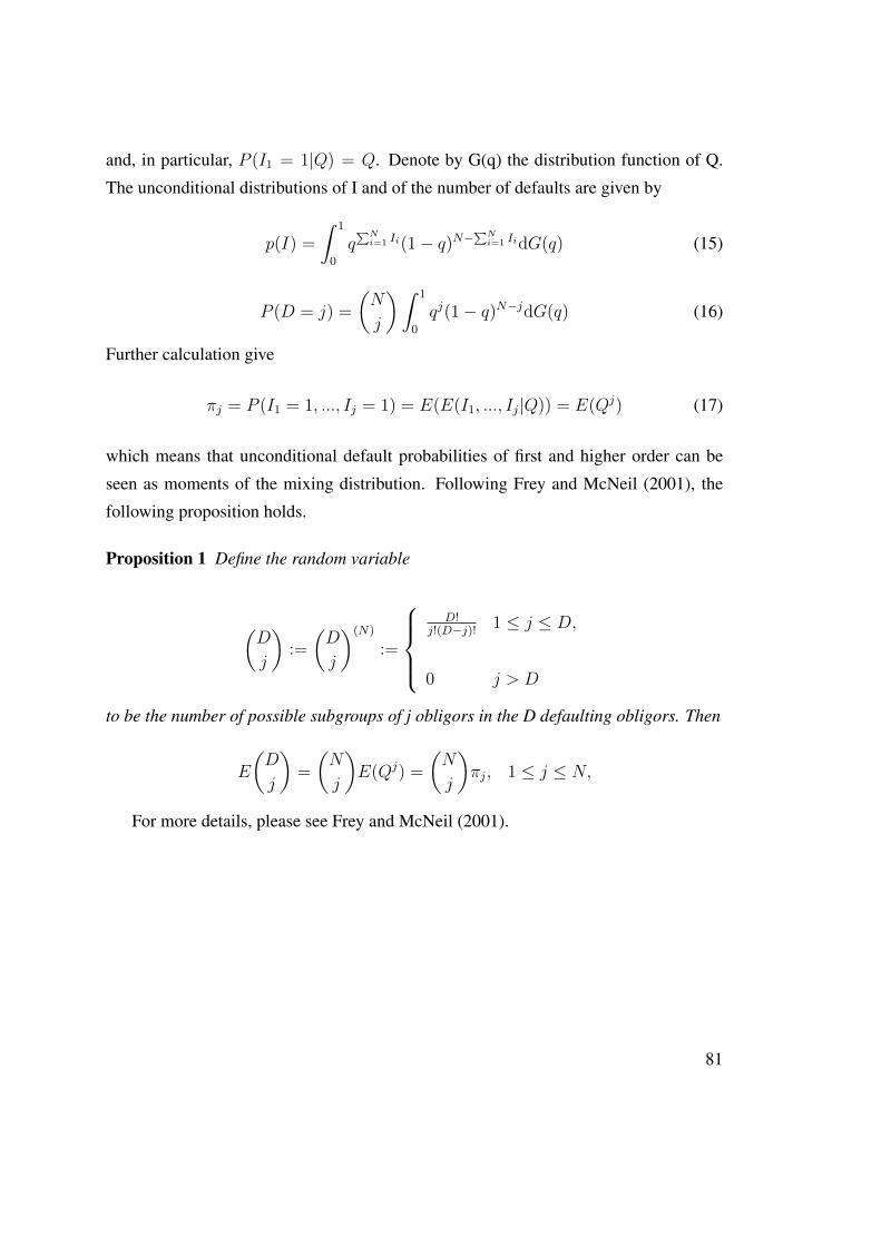
and, in particular, P (I1 = 1|Q) = Q. Denote by G(q) the distribution function of Q.
The unconditional distributions of I and of the number of defaults are given by
p(I) =
∫ 1
0
q∑Ni=1 Ii(1− q)N−
∑Ni=1 IidG(q) (15)
P (D = j) =
(N
j
)∫ 1
0
qj(1− q)N−jdG(q) (16)
Further calculation give
πj = P (I1 = 1, ..., Ij = 1) = E(E(I1, ..., Ij|Q)) = E(Qj) (17)
which means that unconditional default probabilities of first and higher order can be
seen as moments of the mixing distribution. Following Frey and McNeil (2001), the
following proposition holds.
Proposition 1 Define the random variable
(D
j
):=
(D
j
)(N)
:=
D!
j!(D−j)! 1 ≤ j ≤ D,
0 j > D
to be the number of possible subgroups of j obligors in the D defaulting obligors. Then
E
(D
j
)=
(N
j
)E(Qj) =
(N
j
)πj, 1 ≤ j ≤ N,
For more details, please see Frey and McNeil (2001).
81

Appendix B
82
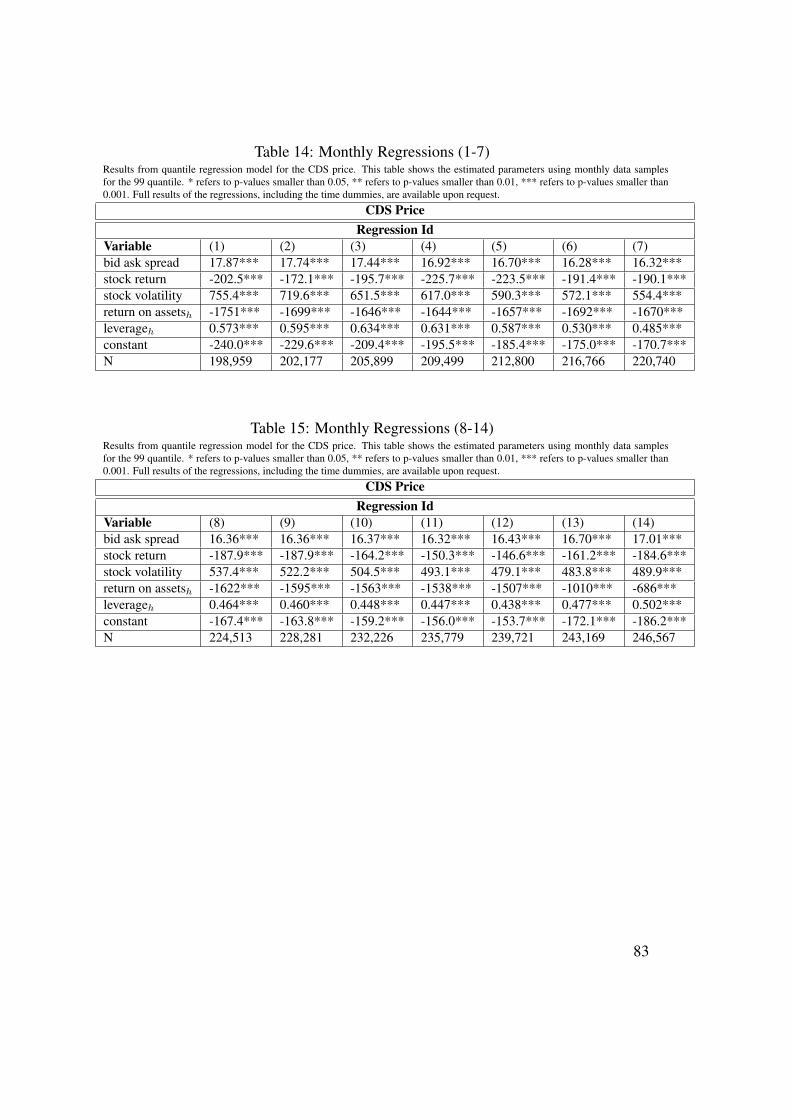
Table 14: Monthly Regressions (1-7)Results from quantile regression model for the CDS price. This table shows the estimated parameters using monthly data samplesfor the 99 quantile. * refers to p-values smaller than 0.05, ** refers to p-values smaller than 0.01, *** refers to p-values smaller than0.001. Full results of the regressions, including the time dummies, are available upon request.
CDS PriceRegression Id
Variable (1) (2) (3) (4) (5) (6) (7)bid ask spread 17.87*** 17.74*** 17.44*** 16.92*** 16.70*** 16.28*** 16.32***stock return -202.5*** -172.1*** -195.7*** -225.7*** -223.5*** -191.4*** -190.1***stock volatility 755.4*** 719.6*** 651.5*** 617.0*** 590.3*** 572.1*** 554.4***return on assetsh -1751*** -1699*** -1646*** -1644*** -1657*** -1692*** -1670***leverageh 0.573*** 0.595*** 0.634*** 0.631*** 0.587*** 0.530*** 0.485***constant -240.0*** -229.6*** -209.4*** -195.5*** -185.4*** -175.0*** -170.7***N 198,959 202,177 205,899 209,499 212,800 216,766 220,740
Table 15: Monthly Regressions (8-14)Results from quantile regression model for the CDS price. This table shows the estimated parameters using monthly data samplesfor the 99 quantile. * refers to p-values smaller than 0.05, ** refers to p-values smaller than 0.01, *** refers to p-values smaller than0.001. Full results of the regressions, including the time dummies, are available upon request.
CDS PriceRegression Id
Variable (8) (9) (10) (11) (12) (13) (14)bid ask spread 16.36*** 16.36*** 16.37*** 16.32*** 16.43*** 16.70*** 17.01***stock return -187.9*** -187.9*** -164.2*** -150.3*** -146.6*** -161.2*** -184.6***stock volatility 537.4*** 522.2*** 504.5*** 493.1*** 479.1*** 483.8*** 489.9***return on assetsh -1622*** -1595*** -1563*** -1538*** -1507*** -1010*** -686***leverageh 0.464*** 0.460*** 0.448*** 0.447*** 0.438*** 0.477*** 0.502***constant -167.4*** -163.8*** -159.2*** -156.0*** -153.7*** -172.1*** -186.2***N 224,513 228,281 232,226 235,779 239,721 243,169 246,567
83
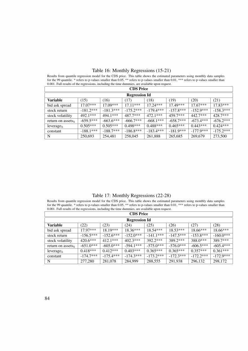
Table 16: Monthly Regressions (15-21)Results from quantile regression model for the CDS price. This table shows the estimated parameters using monthly data samplesfor the 99 quantile. * refers to p-values smaller than 0.05, ** refers to p-values smaller than 0.01, *** refers to p-values smaller than0.001. Full results of the regressions, including the time dummies, are available upon request.
CDS PriceRegression Id
Variable (15) (16) (17) (18) (19) (20) (21)bid ask spread 17.07*** 17.09*** 17.11*** 17.24*** 17.49*** 17.67*** 17.83***stock return -181.2*** -181.3*** -175.2*** -179.4*** -157.8*** -152.9*** -158.3***stock volatility 492.1*** 494.1*** 487.7*** 472.1*** 459.7*** 442.7*** 428.7***return on assetsh -659.5*** -663.6*** -666.7*** -668.1*** -658.7*** -673.4*** -676.2***leverageh 0.505*** 0.505*** 0.498*** 0.488*** 0.465*** 0.443*** 0.424***constant -188.1*** -188.7*** -186.8*** -183.4*** -181.9*** -177.9*** -175.2***N 250,693 254,481 258,045 261,888 265,685 269,679 273,500
Table 17: Monthly Regressions (22-28)Results from quantile regression model for the CDS price. This table shows the estimated parameters using monthly data samplesfor the 99 quantile. * refers to p-values smaller than 0.05, ** refers to p-values smaller than 0.01, *** refers to p-values smaller than0.001. Full results of the regressions, including the time dummies, are available upon request.
CDS PriceRegression Id
Variable (22) (23) (24) (25) (26) (27) (28)bid ask spread 17.97*** 18.19*** 18.36*** 18.54*** 18.53*** 18.66*** 18.66***stock return -156.5*** -152.6*** -152.0*** -141.1*** -147.5*** -153.8*** -160.0***stock volatility 420.6*** 412.1*** 402.3*** 392.2*** 389.2*** 388.0*** 389.7***return on assetsh -651.0*** -605.0*** -594.1*** -575.0*** -576.0*** -606.5*** -605.4***leverageh 0.418*** 0.412*** 0.403*** 0.365*** 0.365*** 0.357*** 0.361***constant -174.7*** -175.4*** -174.3*** -173.2*** -172.3*** -172.2*** -172.9***N 277,280 281,078 284,999 288,555 291,938 296,132 298,172
84
Bibliography
[1] Abid, F., and N. Naifar (2008), CDO Parameters Estimation Using Market Prices,International Research Journal of Finance and Economics , 18, 85-95.
[2] Akhavein, J.D., Kocagil, A.E., and M. Neugebauer (2005), A Comparative Empir-ical Study of Asset Correlations, Working Paper, Fitch.
[3] Allen, D.E., Boffey, R.R., and R.J. Powell (2012), Applying Quantile Regressionto Industry Default Risk in Europe, International Review of Business ResearchPapers, Vol. 8, No. 4, 20-29.
[4] Angelidis, T., Benos, A., and S.A. Degiannakis (2004), The Use of GARCH Mod-els in VaR Estimation, Statistical Methodology, Vol. 1, No. 2, 105-128.
[5] Artzner, P., Delbaen, F., Eber, J., and D.Heath (1999), Coherent Risk Measures,Journal of Mathematical Finance, Vol. 9, No. 3, 203-228.
[6] Bannier, C.E., and D.N. Hansel (2007), Determinants of banks’ engagement inloan securitization, Working Paper, www.papers.ssrn.com.
[7] Baur, D.G. (2013), The structure and degree of dependence: A quantile regressionapproach, Journal of Banking and Finance, Vol. 37, 786-798.
[8] Bauwens, L., Laurent, S., and J.V.K. Rombouts (2006), Multivariate GARCHmodels: a survey, Journal of Applied Econometrics, Vol. 21, No. 1, 79109.
[9] Berkowitz, J., and J. O’Brien (2002), How accurate are the value-at-risk models atcommercial banks?, Journal of Finance, Vol. 57, 1093-1111.
[10] Bollerslev, T. (1986), Generalized Autoregressive Conditional Heteroskedasticity,Journal of Econometrics, Vol. 31, 307-327.
[11] Bollerslev, T. and J. Wooldridge (1992), Quasi-maximum likelihood estima-tion and inference in dynamic models with time-varying covariances, Journal ofEconometric Reviews, Vol.11, No. 2, 143-172.
[12] Bongaerts, D., de Jong, F., and J. Driessen, (2011), Derivative Pricing with Liq-uidity Risk: Theory and Evidence from the Credit Default Swap Market, Journalof Finance, Vol.66, No. 1, 203240.
[13] Bystrom, H. (2005), Credit default swaps and equity prices: the iTraxx CDS indexmarket, Working Paper, Lund University.
85
[14] Campbell, J.Y., Hilscher, J., and J. Szilagyi (2008), In Search of Distress Risk, TheJournal of Finance, Vol. LXIII, No. 6, 2899-2939.
[15] Campbell, S. D. (2005), A Review of Backtesting and Backtesting Procedures,Board of Governors of the Federal Reserve System (U.S.) Working Paper.
[16] Chen, C.W.S., Gerlach, R., Hwang, B.B.K, and M. McAleer (2012), ForecastingValue-at-Risk using nonlinear regression quantiles and the intra-day range, Inter-national Journal of Forecasting, Vol. 28, 557-574.
[17] Chernih, A., Vanduffel, S., and L. Henrard (2006), Asset Correlations: A Lit-erature Review and Analysis of the Impact of Dependent Loss Given Defaults,Working Paper, www.defaultrisk.com.
[18] Chernozhukov, V., and L. Umantsev (2000), Conditional Value-at-Risk: Aspectsof Modeling and Estimation, Working Paper, papers.ssrn.com.
[19] Cherubini, U., Luciano, E., and W. Vecchiato (2004), ”Copula Methods in Fi-nance”, John Wiley & Sons.
[20] Christoffersen P. (1998), Evaluating Interval Forecasts, International EconomicReview, Vol. 39, No. 4, 841-862.
[21] Coad, A., and R. Rao (2006), Innovation and market value: a quantile regressionanalysis, Economics Bulletin, Vol. 15, No. 13, 1-10.
[22] Cochrane, J.H. (2005), Writing Tips for Ph. D. Students, Working Paper,http://gsbwww.uchicago.edu/fac/john.cochrane/research/Papers/.
[23] Coval, J.D., Jurek, J.W., and E. Stafford (2008), The Economics of StructuredFinance, Working Paper, http://papers.ssrn.com.
[24] Crouhy, M., Galai, D., and R. Mark (2000), A Comparative Analysis of CurrentCredit Risk Models, Journal of Banking & Finance, Vol. 24, No. 1-2, 59-117.
[25] Danielsson, J., and C.G. de Vries (2000), Value-at-risk and extreme returns, An-nales d’Economie et de Statistique, Vol. 60, 239-270.
[26] Das, S.R., Duffie, D., Kapadia, N., and L. Saita (2007), Common Failings: HowCorporate Defaults are Correlated, Journal of Finance, Vol. 62, No. 1, 93-117.
[27] Das, S.R., Hanouna, P., and A. Sarin (2009), Accounting-based versus market-based cross-sectional models of CDS spreads, Journal of Banking and FinanceVol. 33, 719730.
[28] De Servigny, A., and O. Renault (2002a), Default correlation: Empirical evidence,Standard and Poor’s Risk Solutions - Presentation.
[29] De Servigny, A., and O. Renault (2002b), Default correlation: Empirical evidence,Working Paper, Standard and Poor’s.
[30] De Servigny, A., and O. Renault (2003), Correlation evidence, RISK, Vol. 16, No.7, 90-94.
86
[31] Debuysscher, A., and M. Szego (2003), The Fourier Transform Method - Technicaldocument, Working Paper, Moody’s Investors Service.
[32] Demarta, S., and A.J. McNeil (2004), The t Copula and Related Copulas, Interna-tional Statistical Review, Vol. 73, No. 1, 111-129.
[33] Diebold, F. X., Schuerman, T., and J.D. Stroughair (1998), Pitfalls and Opportu-nities in the Use of Extreme Value Theory in Risk Management, Working Paper98-10, Wharton School, University of Pennsylvania.
[34] Dorey, M., Joubert, P., and C.P. Vencatasawmy (2005), Modelling Dependencies:an Overview, Presentation to the Finance and Investment Conference.
[35] Duffie, D. (2008), Innovations in credit risk transfer: Implications for financialstability, Working Paper, BIS.
[36] Duffie, D., Eckner, A., Horel, G., and L. Saita (2009), Frailty Correlated Default,Journal of Finance, Vol. 64, No. 5, 2089-2123.
[37] Dullmann, K., Kull, J., and M. Kunisch (2008), Estimating asset correlations fromstock prices or default rates which method is superior?, Working Paper, DeutscheBundesbank.
[38] Embrechts, P., Klupperberg, C., and T. Mikosch (1997), Modelling ExtremalEvents for Insurance and Finance, Springer.
[39] Engle, R.F. (2001), GARCH 101: The Use of ARCH/GARCH Models in AppliedEconometrics, The Journal of Economic Perspectives, Vol. 15, No. 4, 157-168.
[40] Engle, R.F., and S. Manganelli (1999), CAViaR: Conditional Value at Risk byQuantile Regression, Working Paper, NBER Working Paper Series.
[41] Engle, R.F., and S. Manganelli (2004), CAViaR: Conditional Autoregressive Valueat Risk by Regression Quantiles, Journal of Business & Economic Statistics, Vol.22, No. 4, 367-381.
[42] Ericsson, J., Jacobs, K., and R. Oviedo (2009), The determinants of credit de-fault swap premia, Journal of Financial and Quantitative Analysis, Vol. 44, No. 1,109132.
[43] Fender, I., and J. Kiff (2004), CDO rating methodology: Some thoughts on modelrisk and its implications, Working Paper, BIS.
[44] Frey, R., McNeil, A.J., and M.A. Nyfeler (2001), Modelling Dependent Defaults:Asset Correlations Are Not Enough!, Working Paper, www.defaultrisk.com.
[45] Frey, R., and A.J. McNeil (2001), Modelling Dependent Defaults, ETH E-Collection, http://e-collection.ethbib.ethz.ch/show?type=bericht&nr=273.
[46] Frey, R., and A.J. McNeil (2003), Dependent Defaults in Models of PortfolioCredit Risk, Journal of Risk, Vol. 6, No. 1, 59-92.
[47] Gaglianone, W.P, Renato Lima, L., and O. Linton (2008), Evaluating Value-at-Risk Models via Quantile Regressions, Working Paper, Banco Central do Brasil.
87
[48] Garcia, J., Dewyspelaere, T., Langendries, R., Leonard, L., and T. Van Ges-tel (2004), On Rating Cash-Flow CDO’s using BET technique, Working Paper,www.defaultrisk.com.
[49] Gebka, B., and M.E. Wohar (2013), Causality between trading volume and re-turns: Evidence from quantile regressions, International Review of Economics andFinance, Vol. 27, 144-159.
[50] Glosten, L.R., Jagannathan, R., and D.E. Runkle (1993), On the relation betweenthe expected value and the volatility of the nominal excess return on stocks, Jour-nal of Finance, Vol. 48, 1779-1801.
[51] Goderis, B., Marsh, I.W., Castello, J.V., and W. Wagner. (2007), BankBehavior with Access to Credit Risk Transfer Markets, Working Paper,www.defaultrisk.com.
[52] Halbleib, R., and W. Pohlmeier (2012), Improving the value at risk forecasts: The-ory and evidence from the financial crisis, Journal of Economic Dynamics & Con-trol, Vol. 26, 1212-1228.
[53] Hamerle, A., and D. Rosch (2005), Misspecified copulas in credit risk models:how good is Gaussian, Journal of Risk, Vol. 8, No. 1, 41-58.
[54] Hansel, D.N., and J.P. Krahnen (2007), Does credit securitization reducebank risk? Evidence from the European CDO market, Working Paper,www.papers.ssrn.com.
[55] Haugh, M. (2004), The Monte Carlo Framework, Examples from Fi-nance and Generating Correlated Random Variables, Unpublished manuscript,http://www.columbia.edu.
[56] Heitfield, E. (2009), Parameter Uncertainty and the Credit Risk of CollateralizedDebt Obligations, Working Paper, www.papers.ssrn.com.
[57] Hoechle, D. (2007), Robust standard errors for panel regressions with crosssec-tional dependence, The Stata Journal, Vol. 7, No. 3, 281-312.
[58] Hrvatin, R.V., and M. Neugebauer (2004), Default Correlation and Its Effect onPortfolios of Credit Risk, Working Paper, Fitch Ratings.
[59] J.P. Morgan (1997), Credit Metrics - Technical Document.
[60] Jobst, N., and A. De Servigny (2005), An Empirical Analysis of Equity DefaultSwaps II: Multivariate Insights, Working Paper, http://papers.ssrn.com.
[61] Jorion, P. (2007), Value at Risk, McGraw-Hill Professional.
[62] Kalemanova, A., Schmid, B., and R. Werner (2007), The Normal Inverse GaussianDistribution for Synthetic CDO Pricing, Journal of Derivatives, Vol. 14, No. 3, 80-93.
[63] Kiff, J. (2004), The basic math of default-mode credit loss distributions, unpub-lished draft, Bank of Canada, Ottawa.
88
[64] Koenker, R., and G. Bassett (1978), Regression Quantiles, Econometrica, Vol. 46,No. 1, 33-50.
[65] Kuester, K., Mittnik, S., and M.S. Paolella (2006), Value-at-Risk Prediction: AComparison of Alternative Strategies, Journal of Financial Econometrics, Vol. 4,No. 1, 53-89.
[66] Kupiec P. (1995), Techniques for Verifying the Accuracy of Risk ManagementModels, Journal of Derivatives, Vol. 3, No. 2, 73-84.
[67] Lando, D., and M.S. Nielsen (2008), Correlation in Corporate Defaults: Contagionor conditional independence?, Working Paper, www.defaultrisk.com.
[68] Lee, B.S., and M.L. Li (2012), Diversification and risk-adjusted performance: Aquantile regression approach, Journal of Banking and Finance, Vol. 36, 2157-2173.
[69] Li, D.X. (1999), On Default Correlation: A Copula Function Approach, Journalof Fixed Income, Vol. 9, No. 4, 43-54.
[70] Longstaff, F.A., and A. Rajan (2007), An Empirical Analysis of the Pricing ofCollateralized Debt Obligations, Journal of Finance, Vol. 63, No. 2, 529-563.
[71] Lopez, J. (1998), Methods for Evaluating Value-at-Risk, Working Paper, FederalReserve Bank of New York Economic Policy Review, issue Oct, 119-124.
[72] Lucas, D.J. (1995), Default Correlation and Credit Analysis, Journal of Fixed In-come, Vol. 4, No. 4, 76-87.
[73] Mahfoudhi, R. (2011), Credit default swap trees, The Journal of Credit Risk, Vol.7, No.3, 337.
[74] Manganelli, S., and R.F. Engle (2001), Value at Risk Models in Finance, WorkingPaper, European Central Bank.
[75] Mashal, R., and A. Zeevi (2002), Beyond Correlation: Extreme Co-movementsBetween Financial Assets, Working Paper, www.defaultrisk.com.
[76] Mashal, R., Naldi, M., and G. Tejwani (2004), The Implications of Implied Corre-lations, RISK, Vol. 17, No. 7, 66-68.
[77] McNeil, A.J, and R. Frey (2000), Estimation of tail-related risk measures for het-eroscedastic financial time series: an extreme value approach, Journal of Empiri-cal Finance, Vol. 7, 271-300.
[78] Meissner, G., Garnier, T., and T. Laute (2008), A comparative analysis of Fitch’s,Moody’s and Standard and Poor’s CDO rating approaches, The Definitive Guidedo CDOs, Risk Books, 507-528.
[79] Merton, R.C. (1974), On the Pricing of Corporate Debt: The Risk Structure ofInterest Rates, Journal of Finance, Vol. 29, No. 2, 449-470.
89
[80] Morkoetter, S., Pleus, J., and S. Westerfeld (2012), The impact of counterpartyrisk on credit default swap pricing dynamics, The Journal of Credit Risk, Vol. 8,No. 1, 63-88.
[81] Morokoff, W.J. (2003), Simulation methods for risk analysis of collateralized debtobligations, Working Paper, Moody’s Investors Service.
[82] Nagpal, K., and R. Bahar (2001), Measuring Default Correlation, Risk, Vol. 14,No. 3, 129132.
[83] Nelson, D. B. (1991), Conditional heteroskedasticity in asset returns: A new ap-proach, Econometrica, Vol. 59, No. 2, 347-370.
[84] Niethammer, C.R., and L. Overbeck (2008), Default Correlations and the effect ofestimation errors on risk figures, Working Paper, www.defaultrisk.com.
[85] O’Kane, D., and S. Turnbull (2003), Valuation of Credit Default Swaps, LehmanBrothers, Quantitative Credit Research, Vol. 2003-Q1/Q2.
[86] Picone, D. (2002), Collateralised Debt Obligations, Working Paper,www.defaultrisk.com.
[87] Pires, P., Pereira, J.P., and L.F. Martins, The complete picture of Credit DefaultSwap spreads - a Quantile Regression approach, European Financial Management,forthcoming.
[88] Raunig, B., and M. Scheicher (2008), A Value at Risk Analysis of Credit DefaultSwaps, Working Paper, European Central Bank.
[89] Robert, S., Default Correlation: An empirical approach, Working Paper, Univer-sity of Applied Sciences BFI Vienna.
[90] Rossignolo, A.F., Fethi, M.D., and M. Shaban (2012), Value-at-Risk models andBasel capital charges Evidence from Emerging and Frontier stock markets, Journalof Financial Stability, Vol. 8, 303-319.
[91] Rubia, A., and L. Sanchis-Marco (2013), On downside risk predictability throughliquidity and trading activity: A dynamic quantile approach, International Journalof Forecasting, Vol. 29, 202-219.
[92] Schweizer, B., and A. Sklar (1983), Probabilistic Metric Spaces, North-Holland/Elsevier.
[93] Sener, E., Baronyan, S., and L.A. Menguturk (2012), Ranking the predictive per-formances of value-at-risk estimation methods, International Journal of Forecast-ing, Vol. 28, 849-873.
[94] Sklar, A. (1959), Fonctions de Rpartition n Dimensions et Leurs Marges, Publi-cations de L’Institut de Statistique de L’Universit de Paris, No. 8, 229-231.
[95] Stulz, R. (2009), Credit Default Swaps and the Credit Crisis, ECGI finance work-ing paper 264/2009.
90
[96] Tang, D.Y., and H. Yan (2007), Liquidity and credit default swap spreads, WorkingPaper, www.defaultrisk.com.
[97] Taylor, J.W. (1999), A Quantile Regression Approach to Estimating the Distribu-tion of Multiperiod Returns, Journal of Derivatives, Vol. 7, No. 1, 64-78.
[98] Weissbach, R., Rosenow, B., and F. Altrock (2004), Modelling Correlations inPortfolio Credit Risk, Working Paper, www.defaultrisk.com.
[99] Witt, G. (2004), Moody’s Correlated Binomial Default Distribution, Working Pa-per, Moody’s Investors Service.
[100] Wooldridge, J.M. (2002), Econometric Analysis of cross section and panel data,MIT Press.
[101] Zeliade Systems (2009), ”CDOs: How far should we depart from Gaussian cop-ulas?”, Working Paper, http://www.zeliade.com.
[102] Zeng, B., and J. Zhang (2001), An Empirical Assessment of Asset CorrelationModels, Working Paper, KMV.
[103] Zhang, B.Y., Zhou, H., and H. Zhu (2005), Explaining Credit Default SwapSpreads with Equity Volatility and Jump Risks of Individual Firms, Working Pa-per, BIS Working Papers No 181.
91