Embed Size (px)
Citation preview
University of Alberta
Evaluation of SI-HCCI-SI Mode-Switching Using Conventional Actuation on aCNG Engine
by
Jason Bradley Boddez
A thesis submitted to the Faculty of Graduate Studies and Research in partialfulfillment of the requirements for the degree of
Master of Science
Department of Mechanical Engineering
©Jason Bradley BoddezSpring 2011
Edmonton, Alberta
Permission is hereby granted to the University of Alberta Libraries to reproduce single copies of this thesis andto lend or sell such copies for private, scholary or scientific research purposes only. Where the thesis is convertedto, or otherwise made available in digital form, the University of Alberta will advise potential users of the thesis
of these terms.
The author researves all other publication and other rights in association with the copyright in the thesis and,except as herein before provided, neither the thesis nor any substantial portion thereof may be printed or
otherwise reproduced in any material form whatsoever without the author’s prior written permission.
Abstract
Homogeneous Charge Compression Ignition (HCCI) operation is de-
sirable for its high thermal efficiency and low emissions of NOx and
particulates. Difficulty with cold starting and maximum achievable
speed/load highlight the desire for mode-switching to traditional spark
ignition (SI) operation.
Mode-switching between SI and HCCI is investigated using only actu-
ation of throttle, CNG injector pulse width, and CNG injection timing
on a single cylinder CFR engine. Open-loop control achieves a one cy-
cle mode-switch between two adjustable IMEP levels. Sequences are
repeatable as demonstrated by 10 mode-switches with the same inputs.
Performance is evaluated using a developed mode-switch performance
criterion (MSPC) by considering duration between steady-states of op-
eration, smoothness of IMEP, and knock based on maximum rate of
pressure rise. Comparing the results with subjective analysis (the cur-
rent standard) reveals good correlation. Throughout development, mode-
switching performance is shown to improve by a factor of 60.

Acknowledgements
I wish to thank my supervisors, Dr. David Checkel and Dr. Bob Koch,
for their technical and financial support. They have made this endeavor
a very fulfilling experience that I will benefit from for many years to
come.
Also, I would like to thank the staff in the Mechanical Engineering De-
partment for their assistance and expertise, namely Bernie Faulkner,
Rick Conrad, and Roger Marchand. Your contributions and involve-
ment were greatly appreciated.
To my co-researchers and friends, Ahmad, Ali, Dan, Dallin, Darren,
Gillian, Mahdi, Masoud, Michael, Roberto, Rory, and many others,
thank you for your assistance and providing an enjoyable learning envi-
ronment.
And last but not least, I must acknowledge Colleen, my parents (Walter
and Jeannine), family, and friends for their never ending support and
encouragement.
Table of Contents
1 Introduction 1
1.1 Research Objective . . . . . . . . . . . . . . . . . . . . . . . . . . . 2
1.2 Thesis Outline . . . . . . . . . . . . . . . . . . . . . . . . . . . . . . 2
1.3 Contributions . . . . . . . . . . . . . . . . . . . . . . . . . . . . . . 3
2 Background Information 4
2.1 HCCI Fundamentals . . . . . . . . . . . . . . . . . . . . . . . . . . 4
2.1.1 Benefits . . . . . . . . . . . . . . . . . . . . . . . . . . . . . 5
2.1.2 Challenges . . . . . . . . . . . . . . . . . . . . . . . . . . . . 5
2.1.2.1 Combustion Timing Control . . . . . . . . . . . . . 5
2.1.2.2 Load/Speed Limitations . . . . . . . . . . . . . . . 6
2.1.2.3 Cold Starting . . . . . . . . . . . . . . . . . . . . . 7
2.1.2.4 Low Temperature Exhaust Gases . . . . . . . . . . 7
2.1.2.5 HC and CO Emissions . . . . . . . . . . . . . . . . 8
2.1.3 Natural Gas HCCI . . . . . . . . . . . . . . . . . . . . . . . 8
2.2 SI-HCCI-SI Mode-Switching . . . . . . . . . . . . . . . . . . . . . . 9
2.2.1 Existing Strategies . . . . . . . . . . . . . . . . . . . . . . . 10
2.2.2 Proposed Strategy With Conventional Actuation . . . . . . 11
2.2.3 Mode-Switching Effectiveness . . . . . . . . . . . . . . . . . 11
3 Experimental Setup and Methodology 13
3.1 CFR Engine Testbed . . . . . . . . . . . . . . . . . . . . . . . . . . 13
3.1.1 Engine Components . . . . . . . . . . . . . . . . . . . . . . 16
3.1.2 Intake System . . . . . . . . . . . . . . . . . . . . . . . . . . 17
3.1.2.1 Modified Intake System and P IVC . . . . . . . . . . 17
3.1.3 Exhaust System . . . . . . . . . . . . . . . . . . . . . . . . . 21
3.1.4 Calculated Equivalence Ratio . . . . . . . . . . . . . . . . . 21
3.1.4.1 CNG Pulse Width Characterization . . . . . . . . . 21
3.1.4.2 Volumetric Efficiency Characterization . . . . . . . 22
3.2 Engine Data-Logging/Analysis/Control Program . . . . . . . . . . . 26
3.2.1 Injection Timing Limitation . . . . . . . . . . . . . . . . . . 28
3.2.2 Effective Compression Ratio . . . . . . . . . . . . . . . . . . 28
3.2.3 TDC Indexing . . . . . . . . . . . . . . . . . . . . . . . . . . 29
3.3 Combustion Analysis . . . . . . . . . . . . . . . . . . . . . . . . . . 30
3.3.1 CA50 . . . . . . . . . . . . . . . . . . . . . . . . . . . . . . 30
3.3.2 IMEP . . . . . . . . . . . . . . . . . . . . . . . . . . . . . . 31
3.3.3 COV IMEP . . . . . . . . . . . . . . . . . . . . . . . . . . . . 32
3.3.4 Maximum Rate of Pressure Rise (ROPR) . . . . . . . . . . . 32
3.4 Test Procedure . . . . . . . . . . . . . . . . . . . . . . . . . . . . . 32
3.5 Mode-Switching Data Plots - Description and Uncertainties . . . . . 34
3.6 Mode-Switching Evaluation . . . . . . . . . . . . . . . . . . . . . . 34
3.6.1 Duration . . . . . . . . . . . . . . . . . . . . . . . . . . . . . 35
3.6.2 Smoothness . . . . . . . . . . . . . . . . . . . . . . . . . . . 38
3.6.3 Knock . . . . . . . . . . . . . . . . . . . . . . . . . . . . . . 38
3.6.4 Misfire . . . . . . . . . . . . . . . . . . . . . . . . . . . . . . 39
3.6.5 Weighting Factors . . . . . . . . . . . . . . . . . . . . . . . . 39
4 SI-HCCI-SI Mode-Switch Results 41
4.1 Steady-State Operating Conditions - Large Manifold . . . . . . . . 41
4.2 SI-HCCI: Intake Pressure - Step Increase . . . . . . . . . . . . . . . 42
4.3 SI-HCCI: Intake Pressure - First-Order Increase . . . . . . . . . . . 51
4.4 SI-HCCI: CNG Injection Timing . . . . . . . . . . . . . . . . . . . 57
4.5 HCCI-SI: Slow Intake Pressure Drop . . . . . . . . . . . . . . . . . 63
4.6 Steady-State Operating Conditions - Small Manifold . . . . . . . . 69
4.7 HCCI-SI: Quick Intake Pressure Drop . . . . . . . . . . . . . . . . . 71
4.8 SI-HCCI: Optimized Scenario . . . . . . . . . . . . . . . . . . . . . 76
4.9 HCCI-SI: Optimized Scenario . . . . . . . . . . . . . . . . . . . . . 82
4.10 Mode-Switching Sensitivity - Repeated SI-HCCI-SI Transitions . . . 87
4.11 Extension to Other Operating Points . . . . . . . . . . . . . . . . . 90
5 Discussion 101
5.1 SI-HCCI-SI Mode-Switching With Conventional Actuators . . . . . 101
5.1.1 Redevelopment of Mode-Switching Control Sequences for An-
other Engine . . . . . . . . . . . . . . . . . . . . . . . . . . 103
5.2 Repeated SI-HCCI-SI Mode-Switching . . . . . . . . . . . . . . . . 105
5.3 Variation in Steady-State IMEP for SI-HCCI Mode-Switching . . . 106
5.4 Variation in Steady-State IMEP for HCCI-SI Mode-Switching . . . 107
5.5 Mode-Switching Performance Criterion (MSPC) . . . . . . . . . . . 109
5.5.1 Weight Factor Justification . . . . . . . . . . . . . . . . . . . 110
5.5.1.1 Option 1 . . . . . . . . . . . . . . . . . . . . . . . 114
5.5.1.2 Option 2 . . . . . . . . . . . . . . . . . . . . . . . 114
5.5.2 Extension of MSPC to Other Scenarios . . . . . . . . . . . . 115
5.5.2.1 Power Demand . . . . . . . . . . . . . . . . . . . . 115
5.5.2.2 Transition of Slow Actuators . . . . . . . . . . . . 115
5.5.2.3 Multiple Cylinders . . . . . . . . . . . . . . . . . . 117
6 Conclusions 119
6.1 SI-HCCI-SI Mode-Switching Through Conventional Actuation . . . 119
6.2 Mode-Switching Performance Criterion (MSPC) . . . . . . . . . . . 120
6.3 Future Work . . . . . . . . . . . . . . . . . . . . . . . . . . . . . . . 121
Bibliography 123
A Effective Compression Ratio 131
B Thermodynamic Loss Angle 133
C Intake Heat Loss Calculation 137
C.1 Heater Manifold Temperature Gradient . . . . . . . . . . . . . . . . 137
C.2 Polytropic Expansion . . . . . . . . . . . . . . . . . . . . . . . . . . 138
C.3 Joule-Thomson Effect . . . . . . . . . . . . . . . . . . . . . . . . . . 139
C.4 Throttle Cooling Lines . . . . . . . . . . . . . . . . . . . . . . . . . 141
C.5 Convection . . . . . . . . . . . . . . . . . . . . . . . . . . . . . . . . 142
C.6 Temperature Downstream of Throttle . . . . . . . . . . . . . . . . . 144
C.7 CNG Injection . . . . . . . . . . . . . . . . . . . . . . . . . . . . . . 144
C.8 Backflow . . . . . . . . . . . . . . . . . . . . . . . . . . . . . . . . . 145
C.9 Discussion . . . . . . . . . . . . . . . . . . . . . . . . . . . . . . . . 146
D Sensor Calibrations 148
D.1 Air Mass Flow . . . . . . . . . . . . . . . . . . . . . . . . . . . . . . 148
D.2 Compressed Natural Gas (CNG) Mass Flow . . . . . . . . . . . . . 149
D.3 Piezoelectric Cylinder Pressure Transducer . . . . . . . . . . . . . . 151
D.4 Gauge Pressure Transducers . . . . . . . . . . . . . . . . . . . . . . 152
D.5 Thermocouples . . . . . . . . . . . . . . . . . . . . . . . . . . . . . 152
D.6 Exhaust Emissions . . . . . . . . . . . . . . . . . . . . . . . . . . . 155
E Uncertainty Analysis 156
E.1 Average Intake Pressure . . . . . . . . . . . . . . . . . . . . . . . . 156
E.2 P IVC . . . . . . . . . . . . . . . . . . . . . . . . . . . . . . . . . . . 157
E.3 CNG Injection Timing and P IVC Sample Location . . . . . . . . . . 158
E.4 CNG Injection Pulse Width . . . . . . . . . . . . . . . . . . . . . . 158
E.5 IMEP . . . . . . . . . . . . . . . . . . . . . . . . . . . . . . . . . . 159
E.6 CA50 . . . . . . . . . . . . . . . . . . . . . . . . . . . . . . . . . . . 159
E.7 ROPR . . . . . . . . . . . . . . . . . . . . . . . . . . . . . . . . . . 160
E.8 Equivalence Ratio . . . . . . . . . . . . . . . . . . . . . . . . . . . . 160
E.8.1 CNG Mass Per Cycle . . . . . . . . . . . . . . . . . . . . . . 161
E.8.2 Air Mass Per Cycle . . . . . . . . . . . . . . . . . . . . . . . 161
F Engine Control Program Details 163
F.1 Channel Configuration . . . . . . . . . . . . . . . . . . . . . . . . . 163
F.2 Program Indexing . . . . . . . . . . . . . . . . . . . . . . . . . . . . 165
G MATLAB Code for MSPC Analysis 169
H Analysis File Summary 172
List of Figures
2.1 Combustion Mode Comparison. . . . . . . . . . . . . . . . . . . . . 5
3.1 Experimental Waukesha CFR engine. . . . . . . . . . . . . . . . . . 14
3.2 Experimental setup schematic diagram. . . . . . . . . . . . . . . . . 15
3.3 Electronic throttle downstream of intake heater. . . . . . . . . . . . 18
3.4 Intake pressure while motoring showing P IVC. . . . . . . . . . . . . 19
3.5 Intake response with direct control of throttle position. . . . . . . . 20
3.6 Throttle trend implemented in Woodward throttle while testing with
both intake manifolds. . . . . . . . . . . . . . . . . . . . . . . . . . 20
3.7 Small intake response with non-linear throttle trend. . . . . . . . . 20
3.8 CNG mass flow rate independence from intake pressure. . . . . . . . 22
3.9 Linear CNG mass flow rate dependence on injection pulse width. . . 23
3.10 Intake pressure response with manifold air supercharged and heated. 24
3.11 Volumetric efficiency while motoring with manifold air supercharged
and heated. . . . . . . . . . . . . . . . . . . . . . . . . . . . . . . . 24
3.12 Volumetric efficiency for Section 4.11. . . . . . . . . . . . . . . . . . 25
3.13 Engine Control Schematic. . . . . . . . . . . . . . . . . . . . . . . . 27
3.14 Possible CNG injection timings. . . . . . . . . . . . . . . . . . . . . 29
3.15 Procedure to determine mode-switch duration. . . . . . . . . . . . . 37
4.1 SI-HCCI - intake pressure step, no feedback control. . . . . . . . . . 45
4.2 SI-HCCI controls/IMEP - intake pressure step, PI control of CNG
PW. . . . . . . . . . . . . . . . . . . . . . . . . . . . . . . . . . . . 46
4.3 SI-HCCI cylinder pressure - intake pressure step. . . . . . . . . . . 47
4.4 SI-HCCI CA50/ROPR - intake pressure step. . . . . . . . . . . . . 47
4.5 IMEP from Section 4.2 to evaluate smoothness for MSPC. . . . . . 49
4.6 SI-HCCI controls/IMEP - throttle position step. . . . . . . . . . . . 53
4.7 SI-HCCI cylinder pressure - throttle position step. . . . . . . . . . . 53
4.8 SI-HCCI CA50/ROPR - throttle position step. . . . . . . . . . . . . 54
4.9 IMEP from Section 4.3 to evaluate smoothness for MSPC. . . . . . 55
4.10 SI-HCCI controls/IMEP - fuel timing adjustment. . . . . . . . . . . 58
4.11 SI-HCCI cylinder pressure - fuel timing adjustment. . . . . . . . . . 59
4.12 SI-HCCI CA50/ROPR - fuel timing adjustment. . . . . . . . . . . . 59
4.13 IMEP from Section 4.4 to evaluate smoothness for MSPC. . . . . . 61
4.14 HCCI-SI controls/IMEP - large manifold. . . . . . . . . . . . . . . . 64
4.15 HCCI-SI cylinder pressure - large manifold. . . . . . . . . . . . . . . 65
4.16 HCCI-SI cylinder pressure - large manifold. . . . . . . . . . . . . . . 65
4.17 IMEP from Section 4.5 to evaluate smoothness for MSPC. . . . . . 67
4.18 HCCI-SI controls/IMEP - small manifold. . . . . . . . . . . . . . . 72
4.19 HCCI-SI cylinder pressure - small manifold. . . . . . . . . . . . . . 73
4.20 HCCI-SI CA50/ROPR - small manifold. . . . . . . . . . . . . . . . 73
4.21 IMEP from Section 4.7 to evaluate smoothness for MSPC. . . . . . 74
4.22 SI-HCCI controls/IMEP - optimized scenario. . . . . . . . . . . . . 77
4.23 SI-HCCI cylinder pressure - optimized scenario. . . . . . . . . . . . 78
4.24 SI-HCCI CA50/ROPR - optimized scenario. . . . . . . . . . . . . . 78
4.25 IMEP from Section 4.8 to evaluate smoothness for MSPC. . . . . . 80
4.26 HCCI-SI controls/IMEP - optimized scenario. . . . . . . . . . . . . 83
4.27 HCCI-SI cylinder pressure - optimized scenario. . . . . . . . . . . . 84
4.28 HCCI-SI CA50/ROPR - optimized scenario. . . . . . . . . . . . . . 84
4.29 IMEP from Section 4.9 to evaluate smoothness for MSPC. . . . . . 85
4.30 Controls/IMEP during repeated SI-HCCI-SI mode-switching. . . . . 88
4.31 CA50/ROPR during repeated SI-HCCI-SI mode-switching. . . . . . 89
4.32 Disturbances experienced during repeated SI-HCCI-SI mode-switching. 89
4.33 SI-HCCI mode-switches showing different power levels during SI op-
eration. . . . . . . . . . . . . . . . . . . . . . . . . . . . . . . . . . 92
4.34 CA50, ROPR, and approximate equivalence ratio for SI-HCCI mode-
switches presented in Figure 4.33. . . . . . . . . . . . . . . . . . . . 93
4.35 SI-HCCI mode-switches showing different power levels during HCCI
operation. . . . . . . . . . . . . . . . . . . . . . . . . . . . . . . . . 94
4.36 CA50, ROPR, and approximate equivalence ratio for SI-HCCI mode-
switches presented in Figure 4.35. . . . . . . . . . . . . . . . . . . . 95
4.37 HCCI-SI mode-switches showing different power levels during SI op-
eration. . . . . . . . . . . . . . . . . . . . . . . . . . . . . . . . . . 96
4.38 CA50, ROPR, and approximate equivalence ratio for HCCI-SI mode-
switches presented in Figure 4.37. . . . . . . . . . . . . . . . . . . . 97
4.39 HCCI-SI mode-switches showing different power levels during HCCI
operation. . . . . . . . . . . . . . . . . . . . . . . . . . . . . . . . . 98
4.40 CA50, ROPR, and approximate equivalence ratio for HCCI-SI mode-
switches presented in Figure 4.39. . . . . . . . . . . . . . . . . . . . 99
5.1 SI-HCCI mode-switching map. . . . . . . . . . . . . . . . . . . . . . 102
5.2 HCCI-SI mode-switching map. . . . . . . . . . . . . . . . . . . . . . 104
5.3 MSPC weight factor comparison. . . . . . . . . . . . . . . . . . . . 110
A.1 Effective compression ratio evaluation using old and new methods. . 132
B.1 Spark noise in cylinder pressure trace is used to locate geometric TDC.134

B.2 Thermodynamic loss angle found using spark noise while motoring. 135
B.3 Thermodynamic loss angle again, but with outlier point removed. . 135
C.1 Air temperature gradient measured downstream of the electric air
heater. . . . . . . . . . . . . . . . . . . . . . . . . . . . . . . . . . . 138
C.2 Intake pressure trends upstream/downstream of throttle during SI. 140
C.3 Intake pressure trends upstream/downstream of throttle during HCCI.140
D.1 Air mass flow calibration. . . . . . . . . . . . . . . . . . . . . . . . 149
D.2 CNG mass flow calibration. . . . . . . . . . . . . . . . . . . . . . . 150
D.3 Dynamic pressure calibration for piezoelectric pressure transducer. . 151
D.4 Piezoelectric cylinder pressure transducer calibration. . . . . . . . . 152
D.5 Intake pressure transducer calibration. . . . . . . . . . . . . . . . . 153
D.6 Exhaust pressure transducer calibration. . . . . . . . . . . . . . . . 153
D.7 Thermocouple calibration. . . . . . . . . . . . . . . . . . . . . . . . 154
E.1 Variation in RPM throughout one engine cycle. . . . . . . . . . . . 158
F.1 Index signals for fuel injection and TDC. . . . . . . . . . . . . . . . 166
List of Tables
3.1 Description of components used in experimental setup. . . . . . . . 14
3.2 Engine specifications. . . . . . . . . . . . . . . . . . . . . . . . . . . 16
3.3 CFR valve timing. . . . . . . . . . . . . . . . . . . . . . . . . . . . 16
3.4 Measurement uncertainty for mode-switching data plots. . . . . . . 35
4.1 Steady-state operating conditions - large manifold. . . . . . . . . . . 43
4.2 MSPC data for Section 4.2. . . . . . . . . . . . . . . . . . . . . . . 50
4.3 MSPC data for Section 4.3. . . . . . . . . . . . . . . . . . . . . . . 56
4.4 MSPC data for Section 4.4. . . . . . . . . . . . . . . . . . . . . . . 62
4.5 MSPC data for Section 4.5. . . . . . . . . . . . . . . . . . . . . . . 68
4.6 Steady-state operating conditions - small manifold. . . . . . . . . . 70
4.7 MSPC data for Section 4.7. . . . . . . . . . . . . . . . . . . . . . . 75
4.8 MSPC data for Section 4.8. . . . . . . . . . . . . . . . . . . . . . . 81
4.9 MSPC data for Section 4.9. . . . . . . . . . . . . . . . . . . . . . . 86
4.10 Steady-state operating conditions for various IMEP levels to mode-
switch between. . . . . . . . . . . . . . . . . . . . . . . . . . . . . . 91
4.11 MSPC data for Section 4.11. . . . . . . . . . . . . . . . . . . . . . . 100
5.1 Alternate MSPC weight factors. . . . . . . . . . . . . . . . . . . . . 110
5.2 MSPC data with alternate weight factors. . . . . . . . . . . . . . . 111
C.1 Temperature reduction due to polytropic expansion across the throt-
tle for several values of n. . . . . . . . . . . . . . . . . . . . . . . . 140
C.2 Heat loss measurements for water cooling lines on throttle actuator. 141
C.3 Calculated air temperatures downstream of throttle. . . . . . . . . . 144
C.4 Calculated mixture temperatures after CNG injection. . . . . . . . 145
C.5 Calculated intake manifold temperatures including backflow. . . . . 146
D.1 California Analytical Instruments emissions analyzers. . . . . . . . . 155
D.2 Emissions calibration gases. . . . . . . . . . . . . . . . . . . . . . . 155
E.1 CA50 uncertainty using Monte Carlo algorithm. . . . . . . . . . . . 160
F.1 National Instruments PCI-MIO-16E-1 (1) input/output description. 163
F.2 National Instruments PCI-MIO-16E-1 (2) input/output description. 164
F.3 National Instruments PCI-MIO-16E-4 input/output description. . . 164
F.4 National Instruments PCI-6220 input/output description. . . . . . . 165
H.1 LabVIEW programs used for engine operation and calibrations. . . 172
H.2 MATLAB programs used to process data and create figures. . . . . 173
Nomenclature
aTDC After Top Dead Center on the compression stroke
bIVO Before Intake Valve Opening
bTDC Before Top Dead Center on the compression stroke
CA50 Crank Angle Degrees @ 50% mass fraction of fuel burned, relative
to Top Dead Center
CI Compression Ignition
CNG Compressed Natural Gas
CO2 Carbon Dioxide
CO Carbon Monoxide
DAQ Data Acquisition
EVC Exhaust Valve Closing
EVO Exhaust Valve Opening
HC Unburned Hydrocarbons
HCCI Homogeneous Charge Compression Ignition
IMEP Indicated Mean Effective Pressure
IVC Intake Valve Closing
IVO Intake Valve Opening
MSPC Mode-Switching Performance Criterion
NOx Oxides of Nitrogen
O2 Oxygen
PI Proportional-Integral Controller
PPC Pulse Per Cycle
PPM Parts Per Million
PPR Pulse Per Revolution
PW Fuel Injector Pulse Width
ROPR Maximum Rate of Pressure Rise in the cylinder
RSS Root Sum of the Squares
SI Spark Ignition
TDC Top Dead Center on the compression stroke
TDLA Thermodynamic Loss Angle
Symbols
β Volumetric thermal expansion coefficient, approximated as 1/T for
ideal fluids [1/K]
δR Uncertainty in the result of a root sum of the squares
δXi Uncertainty of one component being considered in a root sum of
the squares
ηvol Volumetric efficiency [%]
µIMEP trans Average IMEP during a mode-switch, equal to the mid-point be-
tween the two steady-state values [bar]
µIMEP Average of a set of IMEP values [bar]
µMSPC Average MSPC for a set tests [-]
ν Kinematic viscosity [m2/s]
ρmix Mixture density [kg/m3]
σIMEP trans Standard deviation of IMEP during a mode-switch transition [bar]
σIMEP Standard deviation of a set of IMEP values [bar]
σMSPC cyl Standard deviation of MSPC between cylinders on a multiple cylin-
der engine, averaged over a series of tests [-]
σMSPC Standard deviation of MSPC for a set of tests [-]
Aconv Area for convection heat transfer [m2]
a Crank radius [m]
B Cylinder bore [m]
C Polytropic constant [kPa (m3)n]
Cp air Constant pressure specific heat capacity of air [J/g ◦C]
Cp CNG Constant pressure specific heat capacity of CNG [J/g ◦C]
CNG PW Commanded pulse width of CNG injector for one cycle [ms]
COV IMEP trans Transient coefficient of variation of IMEP [%]
COV IMEP Coefficient of variation of IMEP [%]
Duration Number of cycles to complete a mode-switch based on MSPC def-
inition [-]
g Gravitational acceleration [m/s2]
GrD Grashof Number [-]
h Average convection coefficient [W/m2 ◦C]
IMEP actual Experimental IMEP [bar]
IMEP final Steady-state IMEP in operating mode (SI/HCCI) following mode-
switch [bar]
IMEP initial Steady-state IMEP in operating mode (SI/HCCI) before mode-
switch [bar]
IMEP target Desired IMEP [bar]
J Number of tests [-]
k Thermal conductivity [W/m ◦C]
l Connecting rod length [m]
Lc Characteristic length [m]
M Number of cylinders [-]
mAir Mass of air injected for one cycle [mg/cycle]
mCNG Mass of CNG injected for one cycle [mg/cycle]
mAir Mass flow rate of air [g/s]
mCNG Mass flow rate of CNG [g/s]
mres Mass flow rate of residual gases [g/s]
MSPC Mode-Switching Performance Criterion (MSPC) evaluated from
a single test (or average among cylinders in a multiple cylinder
engine) [-]
MSPCcyl MSPC for one cylinder in a multiple cylinder engine [-]
N Engine rotational speed [rev/s]
n Polytropic index [-]
nr Number of revolutions for a complete set of strokes (nr = 2 for a
4-stroke engine) [rev/cycle]
Nu Nusselt number [-]
Num Number of uncertainty components [-]
P Pressure [kPa]
P cyl Cylinder pressure [bar]
P IVC Pressure at IVC [kPa]
Pr Prandtl Number [-]
Qconv Convection heat transfer [W]
Rair Gas constant for air, 287.06 [J/g ◦C]
RCNG Gas constant for CNG (approximated as methane), 518.27 [J/g
◦C]
RaD Rayleigh number [-]
ROPR Maximum rate of pressure rise for one cycle [bar/CAD]
Stabilize Number of cycles after initiating a mode-switch until propagating
knock is reduced below the knock limit of 10 bar/CAD [-]
T Temperature [K]
T∞ Room temperature [K]
Tmix Mixture temperature [K]
T res Residual gas temperature [K]
T s Surface temperature [K]
V Volume [m3]
V cyl Cylinder volume [m3]
Vd Displacement volume [m3]
1
Chapter 1
Introduction
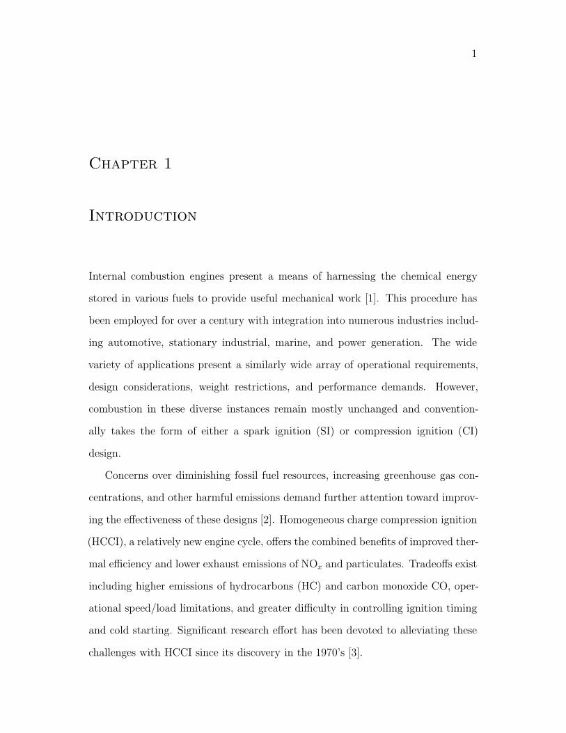
Internal combustion engines present a means of harnessing the chemical energy
stored in various fuels to provide useful mechanical work [1]. This procedure has
been employed for over a century with integration into numerous industries includ-
ing automotive, stationary industrial, marine, and power generation. The wide
variety of applications present a similarly wide array of operational requirements,
design considerations, weight restrictions, and performance demands. However,
combustion in these diverse instances remain mostly unchanged and convention-
ally takes the form of either a spark ignition (SI) or compression ignition (CI)
design.
Concerns over diminishing fossil fuel resources, increasing greenhouse gas con-
centrations, and other harmful emissions demand further attention toward improv-
ing the effectiveness of these designs [2]. Homogeneous charge compression ignition
(HCCI), a relatively new engine cycle, offers the combined benefits of improved ther-
mal efficiency and lower exhaust emissions of NOx and particulates. Tradeoffs exist
including higher emissions of hydrocarbons (HC) and carbon monoxide CO, oper-
ational speed/load limitations, and greater difficulty in controlling ignition timing
and cold starting. Significant research effort has been devoted to alleviating these
challenges with HCCI since its discovery in the 1970’s [3].
CHAPTER 1. INTRODUCTION 2
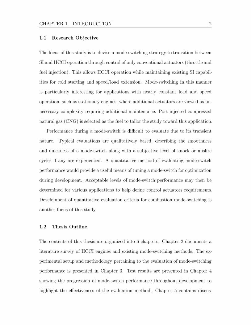
1.1 Research Objective
The focus of this study is to devise a mode-switching strategy to transition between
SI and HCCI operation through control of only conventional actuators (throttle and
fuel injection). This allows HCCI operation while maintaining existing SI capabil-
ities for cold starting and speed/load extension. Mode-switching in this manner
is particularly interesting for applications with nearly constant load and speed
operation, such as stationary engines, where additional actuators are viewed as un-
necessary complexity requiring additional maintenance. Port-injected compressed
natural gas (CNG) is selected as the fuel to tailor the study toward this application.
Performance during a mode-switch is difficult to evaluate due to its transient
nature. Typical evaluations are qualitatively based, describing the smoothness
and quickness of a mode-switch along with a subjective level of knock or misfire
cycles if any are experienced. A quantitative method of evaluating mode-switch
performance would provide a useful means of tuning a mode-switch for optimization
during development. Acceptable levels of mode-switch performance may then be
determined for various applications to help define control actuators requirements.
Development of quantitative evaluation criteria for combustion mode-switching is
another focus of this study.
1.2 Thesis Outline
The contents of this thesis are organized into 6 chapters. Chapter 2 documents a
literature survey of HCCI engines and existing mode-switching methods. The ex-
perimental setup and methodology pertaining to the evaluation of mode-switching
performance is presented in Chapter 3. Test results are presented in Chapter 4
showing the progression of mode-switch performance throughout development to
highlight the effectiveness of the evaluation method. Chapter 5 contains discus-
CHAPTER 1. INTRODUCTION 3
sion of the experimental results. A summary of conclusions and avenues for future
work are given in Chapter 6. Several appendices are included to provide greater
detail of procedures, calibrations, uncertainty analysis, and computer programs
implemented.
1.3 Contributions
Several contributions have been made through the research in this study:� Accurate control of intake pressure and repeatable transients are made pos-
sible with an electronic throttle and reduced intake manifold volume.� Expanding the compression ratio test method to incorporate intake manifold
pressure for consistent readings with variations in atmospheric pressure.� Thermodynamic loss angle is measured experimentally using spark noise, to
predict top dead center (TDC) relative to the location of peak pressure while
motoring, for improved accuracy of combustion analysis.� Development of a LabVIEW based engine control program with synchronized
functions of data logging, on-line combustion analysis, and actuator control,
enabling research toward transient operations.� Providing a simple and quick means of transitioning between SI and HCCI
following cold starting or as required otherwise. Only conventional actuation
of throttle and CNG injection are utilized to allow implementation on engines
without sophisticated controls such as variable valve systems.� Defining a mode-switching performance criterion (MSPC) to allow for quanti-
tative evaluation of mode-switch effectiveness, thus allowing for optimization
and comparison of various control strategies.

4
Chapter 2
Background Information
Discussion is presented here regarding the general operation of HCCI and its asso-
ciated benefits and challenges. Suitability of natural gas for HCCI combustion is
also explored. Mode-switching is presented as a means of cold starting for an HCCI
engine or to widen the limited operating region by reverting to a traditional form
of combustion. The proposed mode-switching strategy implementing only conven-
tional controls is introduced along with its intended purpose. Finally, a quantitative
means of evaluating mode-switching performance is discussed in comparison to the
current subjective standard.
2.1 HCCI Fundamentals
Homogeneous charge compression ignition (HCCI) operates by inducting a homo-
geneous mixture of air and fuel into the combustion chamber before compression
until autoignition. Mixture properties such as fuel composition, equivalence ra-
tio, charge mass, temperature, and residual fraction have a strong influence on
autoignition due to the dependence on thermodynamic properties and chemical
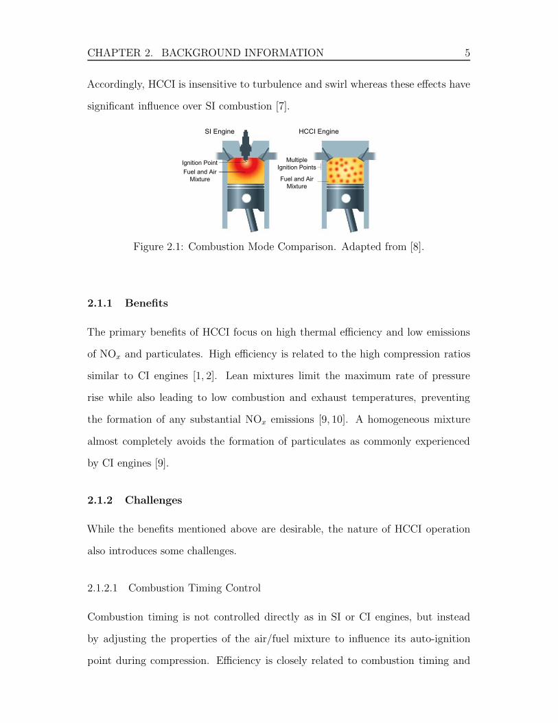
kinetics during combustion [4–6]. Combustion occurs at many points throughout
the compressed mixture simultaneously, demonstrated in Figure 2.1, as opposed to
SI where a spark initiates a flame that propagates across the combustion chamber.
CHAPTER 2. BACKGROUND INFORMATION 5
Accordingly, HCCI is insensitive to turbulence and swirl whereas these effects have
significant influence over SI combustion [7].
SI Engine HCCI Engine
Ignition Point
Fuel and Air
Mixture
Multiple
Ignition Points
Fuel and Air
Mixture
Figure 2.1: Combustion Mode Comparison. Adapted from [8].
2.1.1 Benefits
The primary benefits of HCCI focus on high thermal efficiency and low emissions
of NOx and particulates. High efficiency is related to the high compression ratios
similar to CI engines [1, 2]. Lean mixtures limit the maximum rate of pressure
rise while also leading to low combustion and exhaust temperatures, preventing
the formation of any substantial NOx emissions [9, 10]. A homogeneous mixture
almost completely avoids the formation of particulates as commonly experienced
by CI engines [9].
2.1.2 Challenges
While the benefits mentioned above are desirable, the nature of HCCI operation
also introduces some challenges.
2.1.2.1 Combustion Timing Control
Combustion timing is not controlled directly as in SI or CI engines, but instead
by adjusting the properties of the air/fuel mixture to influence its auto-ignition
point during compression. Efficiency is closely related to combustion timing and

CHAPTER 2. BACKGROUND INFORMATION 6
rate, suggesting that control of this sensitive event is necessary to realize the fuel
efficiency benefit of HCCI operation [2]. Numerical modeling can be used to develop
an understanding of HCCI combustion to predict engine outputs [4,11]. Controllers
are then developed to utilize different actuators to modify ignition timing to an
optimum value, including variable valve timing [12, 13], dual fuels [12–14], split
fuel injection during exhaust negative valve overlap [15], reformer gas addition [16],
intake air temperature [17, 18], and pilot direct injection [19] to name a few.
Of interest among these different options is the range of control possible as well
as the time required for adjustments to be made. Intake temperature, for example,
is commonly referred to as a “slow” actuator as it requires numerous cycles to
vary any significant amount. Fast thermal management installations implementing
two intake air streams, one hot and one cool, can achieve faster response with
some added complexity [17]. On the other hand, “fast” actuators such as fuel
injection pulse width and variable valve systems are able to modify their output on
individual cycles for a high degree of control. Use of these fast responding actuators
is especially preferred when dealing with the added difficulty of disturbances or
changes in operation such as engine speed [20].
2.1.2.2 Load/Speed Limitations
Operational boundaries limit the possible range of power and speed available during
HCCI operation. Stable combustion is restricted between the misfire and knock
limits as imposed by chemical kinetics and the rate of reaction, preventing the large
power range associated with conventional SI engines. Similarly, rate of reaction
imposes limitations on the maximum engine speeds at which combustion timing can
be adjusted to extract useful work [6]. High boost pressures [21], pilot injection [22],
and variable valve timing [23,24] offer some means of expanding the available HCCI
operating region.
CHAPTER 2. BACKGROUND INFORMATION 7
2.1.2.3 Cold Starting
Cold starting is challenging in the sense that typical HCCI operation depends
on several aspects of an operating engine: combustion chamber surfaces are at
a higher temperature in a warm engine to reduce heat loss during compression;
intake air may be heated using coolant or exhaust gases, neither of which are
available in a cold engine; and hot residual gases from previous combustion cycles
promote ignition by heating the mixture and providing radicals to initiate chemical
reactions. Without these conditions on a cold engine, it becomes difficult to achieve
the required autoignition temperature to ignite the air/fuel mixture through HCCI.
Preheating the intake manifold with a natural gas burner allows for starting directly
into HCCI [17], although requires a lengthy period of time and the use of additional
fuel. Using gasoline direct injection, it is possible to ignite one cycle in SI while
motoring and use the hot residual to continue HCCI combustion on subsequent
cycles [15]. Combustion is not ideal during early cycles, but further development
may remedy this situation. This approach, however, does not assist port-injected
engines. Fuels with higher autoignition temperatures, such as natural gas, may
also experience increased difficulty in achieving HCCI combustion in a cold engine
through this approach.
2.1.2.4 Low Temperature Exhaust Gases
Typical HCCI operation involves the use of highly dilute air/fuel mixtures and ex-
haust gas recirculation (EGR) to limit the maximum rate of pressure rise (ROPR).
The resulting low combustion temperatures avoid NOx generation, but low exhaust
temperature becomes a concern when intake heating is implemented to condition
the mixture. It is not feasible to run a large electric heater, as used in many studies
for simplicity, due to a reduction in overall efficiency. Exhaust heat recovery must
be considered with a practical limitation on intake air temperature imposed by the
CHAPTER 2. BACKGROUND INFORMATION 8
operating exhaust and coolant temperatures.
2.1.2.5 HC and CO Emissions
Low temperature combustion and the dependence on chemical kinetics introduces
potential for partial combustion in the peripheral regions. Compressed gas mix-
ture trapped in crevice volumes or situated near combustion surfaces experience
increased heat transfer to the surroundings, reducing mixture temperature below
that achieved by the bulk mixture and leading to incomplete combustion [25]. This
results in higher emissions of hydrocarbons (HC) and carbon monoxide (CO) in
HCCI compared to SI since a larger region is affected. Oxidation catalysts have
been shown to convert these chemical species to less harmful components, namely
CO2 and H2O, with increasing efficiency even with the relatively low HCCI exhaust
temperatures [25, 26].
2.1.3 Natural Gas HCCI
Compressed natural gas (CNG) is an interesting fuel for HCCI as it offers single
stage combustion with quick burn rates [27]. A high autoignition temperature of
approximately 1100 K requires the use of high compression ratio, intake air heating,
hot residual exhaust, or a combination of these to achieve combustion.
Natural gas is a common fuel for stationary applications due to its high availabil-
ity, low cost, and relatively low emissions of CO2. Comparing the overall operating
efficiency of SI and HCCI for power generation suggests that the two may not dif-
fer significantly [28]; however, ongoing development of HCCI is likely to improve
efficiency further while increasingly strict emissions regulations require costly after
treatment of NOx for SI [29], making HCCI a more appealing alternative. Lean
burn SI operation may be implemented to increase thermal efficiency and reduce
NOx emissions, but at the expense of reduced stability and higher emissions of
CHAPTER 2. BACKGROUND INFORMATION 9
CO and HC [30]. All three of these emissions may be dealt with by implement-
ing stoichiometric operation with EGR and a three-way catalyst [31], but strict
control over equivalence ratio is necessary and fuel efficiency is still limited by a
compression ratio necessary to avoid knock. HCCI offers a means of increasing fuel
efficiency with CNG while reducing NOx generation to the point where catalyst
reduction of this emission is unnecessary, leaving only development of a suitable
low temperature oxidation catalyst necessary to manage CO and HC as discussed
above.
2.2 SI-HCCI-SI Mode-Switching
With HCCI prone to issues of cold starting and speed/load limitations, mode-
switching is viewed as a method to realize its benefits in real world applications.
For automotive, sufficient flexibility in control could allow HCCI operation during
low to mid load operation, while relying on traditional SI combustion for cold
starting, idling, high speed, and high load scenarios. Achieving this full integration
of the two combustion modes requires additional actuation beyond conventional
engines, adding to the complexity, cost, and maintenance. On the other hand,
applications such as series hybrid vehicles and stationary industrial uses are exposed
to more predictable operating speeds and loads over a smaller range [32]. Much
of the additional complexity necessary for automotive use may be undesirable if
the narrow operating region is designed specifically for HCCI operation and slower
transitions are deemed acceptable. In these instances, a method of mode-switching
using available actuators is desirable.
Achieving a mode-switch between SI and HCCI generally requires a significant
shift in operating conditions. The mixture must be diluted significantly through
leaner air/fuel mixtures or EGR addition to limit the rate of combustion in HCCI.
Compression temperatures must reach the autoignition point for HCCI to ensue,
CHAPTER 2. BACKGROUND INFORMATION 10
and this may be accomplished through a variety of means depending on the actu-
ators implemented and the desired operating conditions. When transitioning back
to SI, requirements are much simpler. An acceptable air/fuel mixture along with
a suitable spark timing must allow for ignition similar to normal SI operation, and
conditions must not be conducive to knock.
2.2.1 Existing Strategies
Variable valve technology has been the focus of significant mode-switching research.
Cam-profile switching may be implemented to influence mixture quality by chang-
ing the lift and duration of valve events [15,33–35]. Further adjustment of the valve
phasing can provide additional means of control: intake valve timing allows for
quick variation of air induction, and exhaust valve timing can control the amount
of trapped or re-breathed exhaust gases [24, 36–40]. Fully variable valves provide
flexibility of all valve parameters (timing, lift, and duration) for maximum control
over combustion during mode-switching [38,41,42], but with significantly increased
cost and complexity.
Other control schemes have also been tested for their ability to assist or initiate
mode-switching. External EGR has been shown to reduce knock and combustion
noise during the SI-HCCI transition similar to its effect during steady-state HCCI
operation [33]. Early testing with fast thermal management and variable compres-
sion ratio show potential for mode-switching between SI and HCCI by modifying
charge and compression temperatures [43,44]. Dual fuels also offer the capability to
switch between these combustion modes by modifying the mixture’s autoignition
properties [14]. As always, the concern with a dual fuel system is the additional
operator effort and infrastructure required to distribute two different fuels. Re-
former gas produced on-vehicle from a primary fuel offers potential for controlling
HCCI autoignition properties during HCCI operation [4, 16], and could likely aid
CHAPTER 2. BACKGROUND INFORMATION 11
control during a mode-switch as well. However, production of sufficient quantity to
provide the primary fuel during either SI or HCCI operation is likely impractical
or inefficient.
2.2.2 Proposed Strategy With Conventional Actuation
For this study, a method of mode-switching is desired using only conventional ac-
tuators. Fast controls include CNG mass injected per cycle, CNG injection timing,
and throttle angle. Intake temperature and supercharger pressure upstream of the
throttle are maintained throughout the mode-switch. Overlapping steady-state op-
erating points for both SI and HCCI are necessary, with late spark timing and
throttled operation necessary in SI to avoid knock. The ideology of this approach
is that combustion in both modes may not be ideal at the mode-switch conditions,
but will be stable. In a real world application, slow actuators would transition to
the necessary conditions before initiating the mode-switch, then continue to the
desired operating point in the new combustion mode, all while maintaining stable
operation.
2.2.3 Mode-Switching Effectiveness
Successful mode-switching with each method described above can generally be
tuned to provide a smooth transition over a few cycles under the conditions chosen.
Each study contains a different set of operating conditions making comparisons
difficult, and further, the extent of potential mode-switching points throughout
the operating range of both combustion modes is generally not defined. Profiling
the entire SI and HCCI operating region for this purpose is impractical in most re-
search instances, but discussing the limiting conditions and potential for controller
development provides some indication of flexibility comparison between methods.
It can be reasonably assumed that methods implementing actuators with greater
CHAPTER 2. BACKGROUND INFORMATION 12
control (for example, fully variable valves compared to just variable valve timing)
or a greater number of useful actuators (for example, variable valve timing and cam
profile switching as opposed to variable valve timing alone) will ultimately have a
larger range of suitable mode-switching conditions.
Deciding on representative mode-switching conditions to evaluate different con-
trol strategies is application specific, but evaluating performance of any particular
mode-switch should be relatively the same, where a change in combustion mode
(and possibly steady-state power level) is initiated by some change in actuator
values. The actuator control strategy remains a developmental issue specific to
each engine, but engine response is of concern to the end user and may be viewed
similarly for all scenarios.
Fluctuation in IMEP has been suggested to describe the stability of a mode-
switch [40], but this does not factor in other important conditions of duration,
severity, or repeatability. As there is no well established criterion to quantify mode-
switching performance, evaluation is done by means of qualitative descriptions of
“smoothness” and “quickness”. Individual opinions assess the performance of each
set of data differently, leading to inconsistent conclusions. On the other hand,
knock and misfire are defined by more concrete definitions as these events are
commonly discussed with regards to normal operation. The obvious goal is to avoid
undesirable combustion altogether, but if it does occur these are also typically
discussed with subjective descriptions of severity and frequency. Although the
relative impact of these different aspects on engine operation is difficult to quantify,
they may be combined in a consistent way to provide an overall indication of
mode-switching effectiveness. This study develops a mode-switching performance
criterion (MSPC) for qualitative evaluation of mode-switch effectiveness.
13
Chapter 3
Experimental Setup and Methodology
In this chapter, the experimental engine is described along with any modifications
from previous studies by Hosseini [16] and Handford [19]. Two methods of evaluat-
ing intake pressure, cycle averaged and pressure at IVC (P IVC), are introduced. A
new control program for the engine is developed to offer synchronized data logging,
control, and on-line analysis. Combustion parameters for this system are also de-
fined and discussed. Finally, the developed mode-switching effectiveness criteria is
presented.
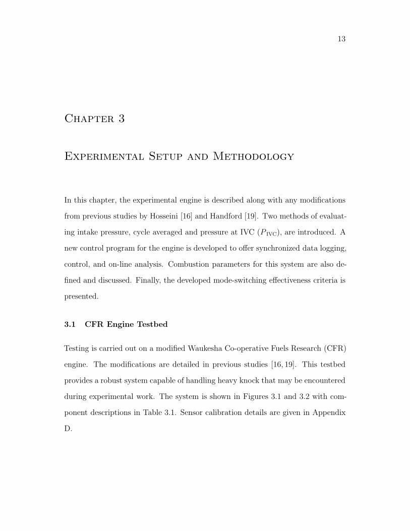
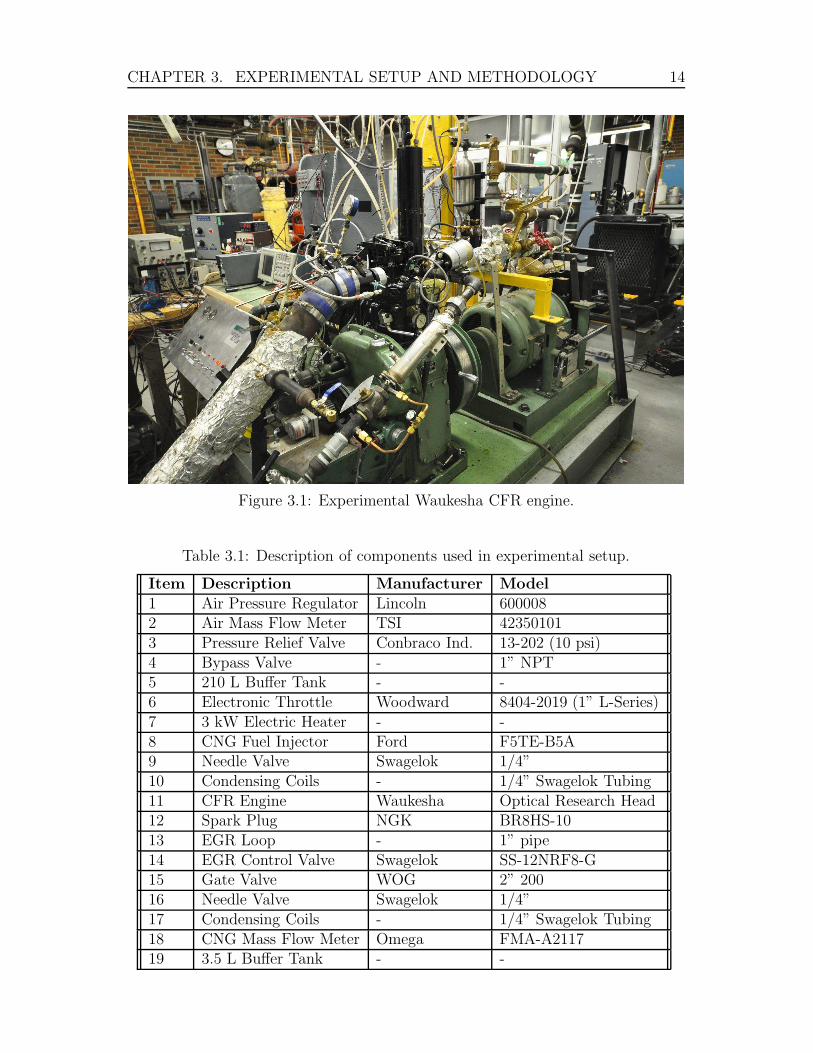
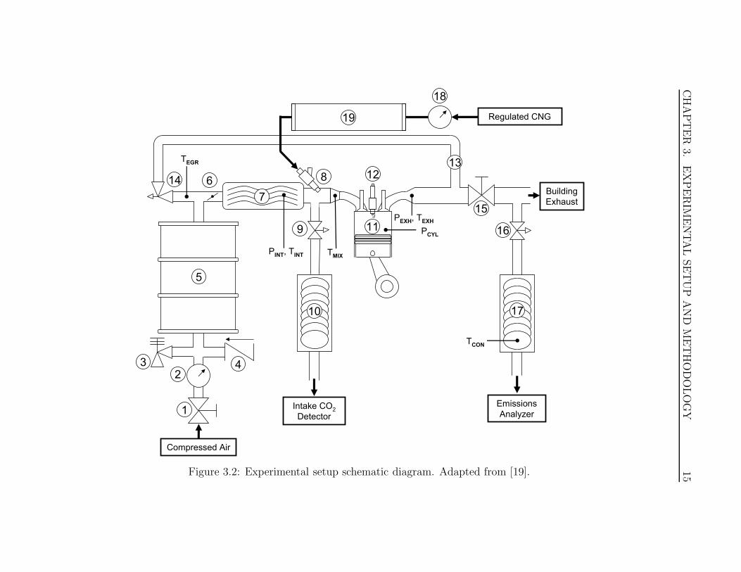
3.1 CFR Engine Testbed
Testing is carried out on a modified Waukesha Co-operative Fuels Research (CFR)
engine. The modifications are detailed in previous studies [16, 19]. This testbed
provides a robust system capable of handling heavy knock that may be encountered
during experimental work. The system is shown in Figures 3.1 and 3.2 with com-
ponent descriptions in Table 3.1. Sensor calibration details are given in Appendix
D.
CHAPTER 3. EXPERIMENTAL SETUP AND METHODOLOGY 14
Figure 3.1: Experimental Waukesha CFR engine.
Table 3.1: Description of components used in experimental setup.
Item Description Manufacturer Model1 Air Pressure Regulator Lincoln 6000082 Air Mass Flow Meter TSI 423501013 Pressure Relief Valve Conbraco Ind. 13-202 (10 psi)4 Bypass Valve - 1” NPT5 210 L Buffer Tank - -6 Electronic Throttle Woodward 8404-2019 (1” L-Series)7 3 kW Electric Heater - -8 CNG Fuel Injector Ford F5TE-B5A9 Needle Valve Swagelok 1/4”10 Condensing Coils - 1/4” Swagelok Tubing11 CFR Engine Waukesha Optical Research Head12 Spark Plug NGK BR8HS-1013 EGR Loop - 1” pipe14 EGR Control Valve Swagelok SS-12NRF8-G15 Gate Valve WOG 2” 20016 Needle Valve Swagelok 1/4”17 Condensing Coils - 1/4” Swagelok Tubing18 CNG Mass Flow Meter Omega FMA-A211719 3.5 L Buffer Tank - -
CHAPTER
3.EXPERIM
ENTALSETUP
AND
METHODOLOGY
15
Compressed Air
Building
Exhaust
Intake CO2
Detector
Emissions
Analyzer1
23 4
5
7
8
9
10
11
13
15
14
16
17
12
TEGR
PINT, T
INT
PCYL
PEXH
, TEXH
TMIX
TCON
6
18
19 Regulated CNG
Figure 3.2: Experimental setup schematic diagram. Adapted from [19].
CHAPTER 3. EXPERIMENTAL SETUP AND METHODOLOGY 16
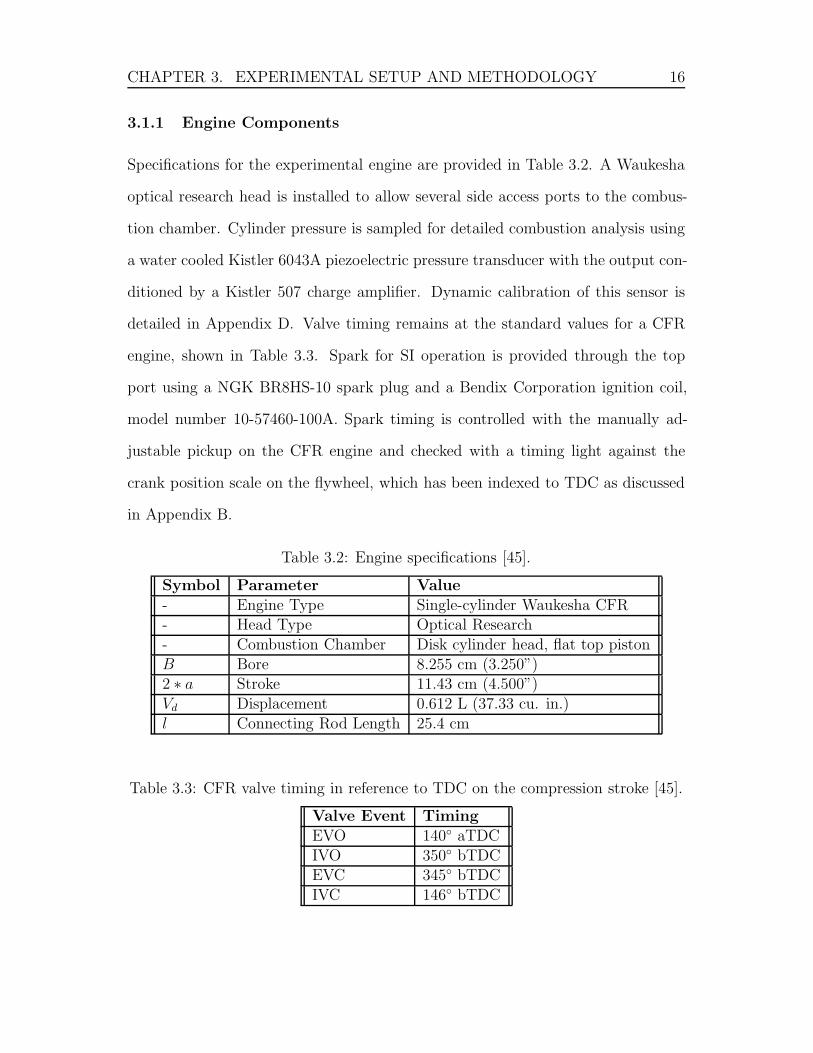
3.1.1 Engine Components
Specifications for the experimental engine are provided in Table 3.2. A Waukesha
optical research head is installed to allow several side access ports to the combus-
tion chamber. Cylinder pressure is sampled for detailed combustion analysis using
a water cooled Kistler 6043A piezoelectric pressure transducer with the output con-
ditioned by a Kistler 507 charge amplifier. Dynamic calibration of this sensor is
detailed in Appendix D. Valve timing remains at the standard values for a CFR
engine, shown in Table 3.3. Spark for SI operation is provided through the top
port using a NGK BR8HS-10 spark plug and a Bendix Corporation ignition coil,
model number 10-57460-100A. Spark timing is controlled with the manually ad-
justable pickup on the CFR engine and checked with a timing light against the
crank position scale on the flywheel, which has been indexed to TDC as discussed
in Appendix B.
Table 3.2: Engine specifications [45].
Symbol Parameter Value- Engine Type Single-cylinder Waukesha CFR- Head Type Optical Research- Combustion Chamber Disk cylinder head, flat top pistonB Bore 8.255 cm (3.250”)2 ∗ a Stroke 11.43 cm (4.500”)Vd Displacement 0.612 L (37.33 cu. in.)l Connecting Rod Length 25.4 cm
Table 3.3: CFR valve timing in reference to TDC on the compression stroke [45].
Valve Event TimingEVO 140◦ aTDCIVO 350◦ bTDCEVC 345◦ bTDCIVC 146◦ bTDC
CHAPTER 3. EXPERIMENTAL SETUP AND METHODOLOGY 17
3.1.2 Intake System
Intake air is supplied from the room through a bypass valve or from compressed
building air if supercharging if desired. Mass flow rate is measured upstream of a
210 L buffer tank in order to reduce flow pulsations and provide accurate readings.
An electronic throttle is installed upstream of a large intake manifold, approxi-
mately 10 L in capacity, containing an electric heater, fuel injection ports, and
various temperature and pressure sensors as indicated. Only room temperature
compressed natural gas (CNG) port fuel injection is utilized in this study. EGR is
not operated in this study.
Due to the large intake manifold volume, the standard 1” (2.54 cm) throttle
body and plate are unable to reduce the intake pressure sufficiently low for SI
operation. So, a sleeve with 5/8” (1.59 cm) inner diameter and custom throttle
plate are fabricated.
Intake pressure is sampled at 1000 Hz using a Valedyne DP15 pressure trans-
ducer. With the large intake manifold, the average reading of all pressure mea-
surements throughout one engine cycle is taken. This provides a relatively linear
response with throttle positions of 0-33% as shown in Figure 3.5a. Larger throt-
tle openings show little effect on air mass flow rate and average intake pressure.
Mode-switching tests with the large 10 L intake manifold maintain throttle posi-
tions within 0-33% with linear demand, as shown in Figure 3.6a, to control air flow
into the engine.
3.1.2.1 Modified Intake System and P IVC
For the results in Section 4.7 and subsequent sections, the intake system is modified
to reduce the throttled intake manifold volume to 0.5 L, or approximately one
displacement volume. Referring to Figure 3.2, this involves moving the throttle
(Item 6) and intake pressure sample point (P INT) to the opposite side of the Item
CHAPTER 3. EXPERIMENTAL SETUP AND METHODOLOGY 18
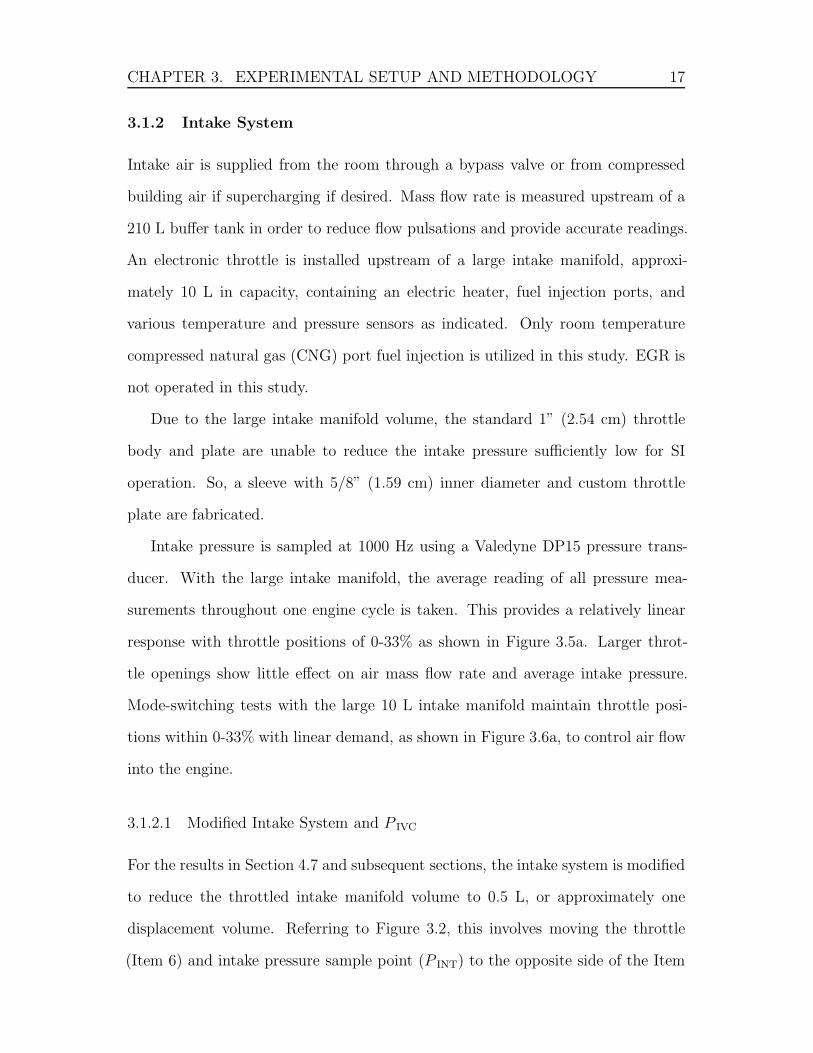
7, a long 8.9cm (3.5”) diameter pipe visible in the lower left of Figure 3.1 containing
the electric air heater. Copper tubing flowing cool tap water is wrapped around the
throttle actuator to prevent overheating in this arrangement, as shown in Figure
3.3. Heat loss through these cooling lines is determined in Appendix C.
Figure 3.3: Electronic throttle positioned downstream of the intake heater forreduced manifold volume. Copper cooling lines prevent actuator overheating.
The smaller manifold volume is required to provide faster control over air de-
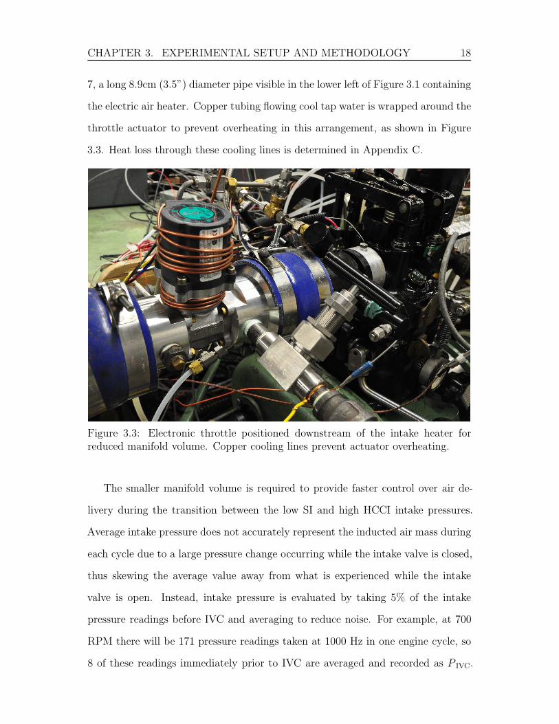
livery during the transition between the low SI and high HCCI intake pressures.
Average intake pressure does not accurately represent the inducted air mass during
each cycle due to a large pressure change occurring while the intake valve is closed,
thus skewing the average value away from what is experienced while the intake
valve is open. Instead, intake pressure is evaluated by taking 5% of the intake
pressure readings before IVC and averaging to reduce noise. For example, at 700
RPM there will be 171 pressure readings taken at 1000 Hz in one engine cycle, so
8 of these readings immediately prior to IVC are averaged and recorded as P IVC.
CHAPTER 3. EXPERIMENTAL SETUP AND METHODOLOGY 19
Since these measurements are time-based, fluctuation in engine speed throughout
the engine cycle leads to an uncertainty of 1.1 CAD with respect to IVC, as calcu-
lated in Appendix E. Figure 3.4 shows the samples averaged for P IVC at different
throttle openings.
0 50 100 150 20020
30
40
50
60
70
80
90
100
Sample Point
Inta
ke P
ress
ure
(kP
a)
Figure 3.4: Intake pressure while motoring at 700 RPM with various throttle open-ings. Highlighted samples are averaged to determine P IVC. Vertical dashed lineindicates IVC.
Controlling throttle position with a PI to maintain a desired intake pressure be-
comes more challenging in this modified setup. Throttle performance is evaluated
by comparing average intake pressure and P IVC with air mass flow rate while motor-
ing at different throttle positions. Strong non-linearities exist as shown in Figure
3.5b, making PI control through either pressure measurement unstable. By im-
plementing a non-linear demand to throttle position calibration in the Woodward
throttle controller, as given in Figure 3.6b, improved linear response is achievable
as visible in Figure 3.7 throughout the entire throttle range, thus removing the 33%
throttle limition with the large manifold. PI control is now suitable to maintain
a desired P IVC, with minor disturbances in supercharger pressure or engine speed
resulting in deviations less than 2 kPa.

CHAPTER 3. EXPERIMENTAL SETUP AND METHODOLOGY 20
0 20 40 60 80 1000
1
2
3
4
5
Position Set Point (%)
Air
Mas
s (m
g/cy
cle)
0
20
40
60
80
100
Inta
ke P
ress
ure
(kP
a)
Air Mass FlowIntake Pressure
(a) Large
0 20 40 60 80 1000
1
2
3
4
5
Position Set Point (%)
Air
Mas
s (m
g/cy
cle)
0
20
40
60
80
100
Pre
ssur
e (k
Pa)
Air Mass FlowIVC PressureIntake Pressure
(b) Small
Figure 3.5: Intake response with direct control of Woodward throttle position forboth intake manifolds.
0 20 40 60 80 1000
20
40
60
80
100
Set Point (%)
Thr
ottle
Pos
ition
(%
)
(a) Large
0 20 40 60 80 1000
20
40
60
80
100
Set Point (%)
Thr
ottle
Pos
ition
(%
)
(b) Small
Figure 3.6: Throttle trend implemented in Woodward throttle while testing withboth intake manifolds.
0 20 40 60 80 1000
1
2
3
4
5
Position Set Point (%)
Air
Mas
s (m
g/cy
cle)
0
20
40
60
80
100
Pre
ssur
e (k
Pa)
Air Mass FlowIVC PressureIntake Pressure
Figure 3.7: Small intake response with non-linear trend programmed in WoodwardThrottle.

CHAPTER 3. EXPERIMENTAL SETUP AND METHODOLOGY 21
3.1.3 Exhaust System
Exhaust gases can exit through the building exhaust system or be routed back to
the intake through the exhaust gas recirculation (EGR) circuit. A gate valve allows
for adjustable back pressure to increase internal EGR fraction and allow EGR while
supercharging. For this study, EGR is not utilized and the gate valve remains fully
open for all tests. Exhaust gas temperature and pressure are measured 10 cm
downstream of the exhaust valve.
3.1.4 Calculated Equivalence Ratio
During testing in Section 4.11, a measure of cycle by cycle mixture quality is
needed to show variation between tests. As no lambda sensor is used and the mass
flow meters do not respond quickly enough, the mixture quality is approximated
by characterizing the fuel delivery with respect to injection pulse width and the
engine’s volumetric efficiency with respect to the measured P IVC. Equivalence ratio
is then calculated using
φ =mCNG/mAir
(mCNG/mAir) stoichiometric(3.1)
where mCNG and mAir are the mass of CNG and air per cycle, respectively. The
associated error is discussed in Appendix E. Alternate options exist to measure
this quantity directly for improved accuracy if desired in future studies [39].
3.1.4.1 CNG Pulse Width Characterization
Fuel delivery is defined by testing the interdependence of fuel injection pulse width
and intake pressure on fuel mass flow rate. Holding the pulse width constant,
intake pressure is varied during SI operation to detect any change in CNG flow
rate. As shown in Figure 3.8, variation from a constant value is minimal and less

CHAPTER 3. EXPERIMENTAL SETUP AND METHODOLOGY 22
than the calibrated accuracy of the CNG mass flow meter. With this information,
CNG mass flow rate is assumed to be primarily dependent on pulse width in the
operating region of interest. Again during SI operation but at a constant intake
pressure, the injection pulse width (CNGPW , specified in [ms]) is varied between
the lean and rich limits covering the expected range for this study. Figure 3.9 shows
a linear trend defined by the best fit line of
mCNG = 1.414CNG PW − 2.375± 1 [mg] (20 : 1) (3.2)
50 55 60 65 70 75
14
14.5
15
15.5
16
16.5
17
17.5
18
PIVC
(kPa)
CN
G M
ass
Per
Inje
ctio
n (m
g/cy
cle)
Figure 3.8: Injected CNG mass during SI operation showing very little dependenceon intake pressure with a constant injector pulse width. Slope of the best fit lineis 0.0013 [mg/cycle kPa].
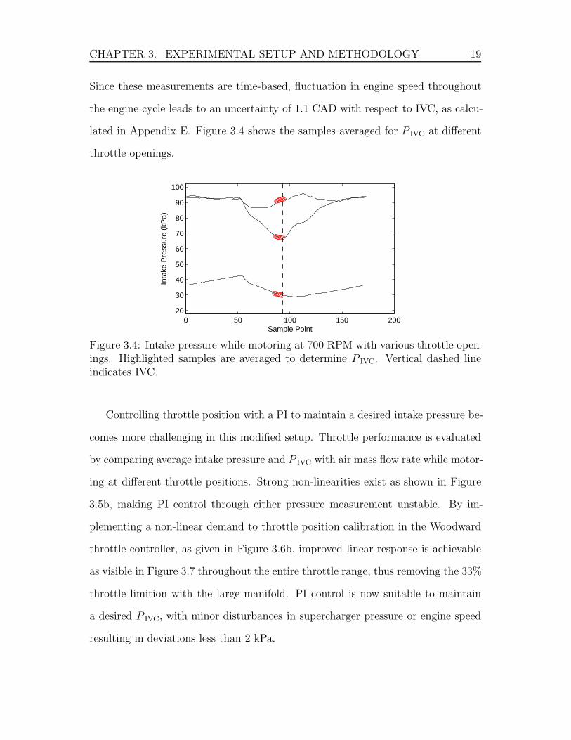
3.1.4.2 Volumetric Efficiency Characterization
Pressure in the intake manifold is correlated with air mass flow rate using volumet-
ric efficiency [1]. P IVC is used instead of the average intake pressure as it provides a
faster response time for approximating the quick and significant changes in air flow
experienced during mode-switching. Since the engine can not be run stably in the
region between SI and HCCI operation, the volumetric efficiency in this range must
be predicted using measurements while motoring. Figure 3.7 presented previously

CHAPTER 3. EXPERIMENTAL SETUP AND METHODOLOGY 23
8 10 12 14 16 18
10
15
20
25
CNG PW (ms)
CN
G M
ass
Per
Inje
ctio
n (m
g/cy
cle)
Figure 3.9: CNG mass flow rate during SI operation showing a linear response withinjection pulse width at a constant intake pressure.
shows the relation between P IVC and air mass flow rate with respect to throttle
position set point; however, to represent the actual test conditions, the procedure
is repeated in Figure 3.10 while motoring with the intake air supercharged and
heated. The density of the mixture (ρmix) is calculated at each of these test points
using
ρmix =mair
mmix
(
P IVC
Rair Tmix
)
+mCNG
mmix
(
P IVC
RCNG Tmix
)
(3.3)
where m is the mass of the indicated constituent, R is the gas constant for air
(287.06 J/g ◦C) or CNG (approximated as methane, 518.27 J/g ◦C), and Tmix is
the mixture temperature. Volumetric efficiencies over the range of throttle positions
can then be determined using
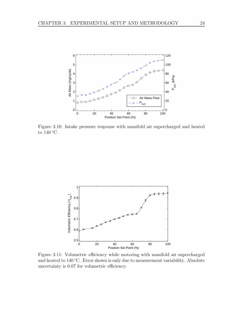
ηvol =mmix nr
N ρmix Vd(3.4)
with mmix and ρmix being the mass flow rate and density of the fuel/air mixture,
respectively, nr being 2 rev/cycle for a 4-stroke engine, N being engine speed, and
Vd being displacement volume [1]. The results of this procedure are shown in Figure
3.11 with respect to throttle position.
CHAPTER 3. EXPERIMENTAL SETUP AND METHODOLOGY 24
0 20 40 60 80 1000
1
2
3
4
5
6
Position Set Point (%)
Air
Mas
s (m
g/cy
cle)
0
20
40
60
80
100
120
PIV
C (
kPa)
Air Mass FlowP
IVC
Figure 3.10: Intake pressure response with manifold air supercharged and heatedto 140 ◦C.
0 20 40 60 80 1000.5
0.6
0.7
0.8
0.9
1
Position Set Point (%)
Vol
umet
ric E
ffici
ency
( η
vol )
Figure 3.11: Volumetric efficiency while motoring with manifold air superchargedand heated to 140 ◦C. Error shown is only due to measurement variability. Absoluteuncertainty is 0.07 for volumetric efficiency.
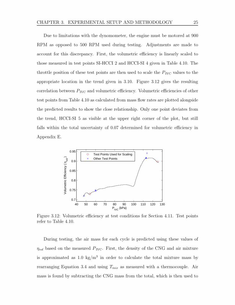
CHAPTER 3. EXPERIMENTAL SETUP AND METHODOLOGY 25
Due to limitations with the dynomometer, the engine must be motored at 900
RPM as opposed to 500 RPM used during testing. Adjustments are made to
account for this discrepancy. First, the volumetric efficiency is linearly scaled to
those measured in test points SI-HCCI 2 and HCCI-SI 4 given in Table 4.10. The
throttle position of these test points are then used to scale the P IVC values to the
appropriate location in the trend given in 3.10. Figure 3.12 gives the resulting
correlation between P IVC and volumetric efficiency. Volumetric efficiencies of other
test points from Table 4.10 as calculated from mass flow rates are plotted alongside
the predicted results to show the close relationship. Only one point deviates from
the trend, HCCI-SI 5 as visible at the upper right corner of the plot, but still
falls within the total uncertainty of 0.07 determined for volumetric efficiency in
Appendix E.
40 50 60 70 80 90 100 110 120 130
0.7
0.75
0.8
0.85
0.9
0.95
PIVC
(kPa)
Vol
umet
ric E
ffici
ency
( η
vol )
Test Points Used for ScalingOther Test Points
Figure 3.12: Volumetric efficiency at test conditions for Section 4.11. Test pointsrefer to Table 4.10.
During testing, the air mass for each cycle is predicted using these values of
ηvol based on the measured P IVC. First, the density of the CNG and air mixture
is approximated as 1.0 kg/m3 in order to calculate the total mixture mass by
rearranging Equation 3.4 and using Tmix as measured with a thermocouple. Air
mass is found by subtracting the CNG mass from the total, which is then used to
CHAPTER 3. EXPERIMENTAL SETUP AND METHODOLOGY 26
recalculate the density. The process is repeated until the error in the calculated
density is less than 0.1%. To confirm the accuracy of this approach, the air mass
flow rate of the other steady-state conditions in Table 4.10 are predicted, with the
results all falling within 1.5% of the measured values.
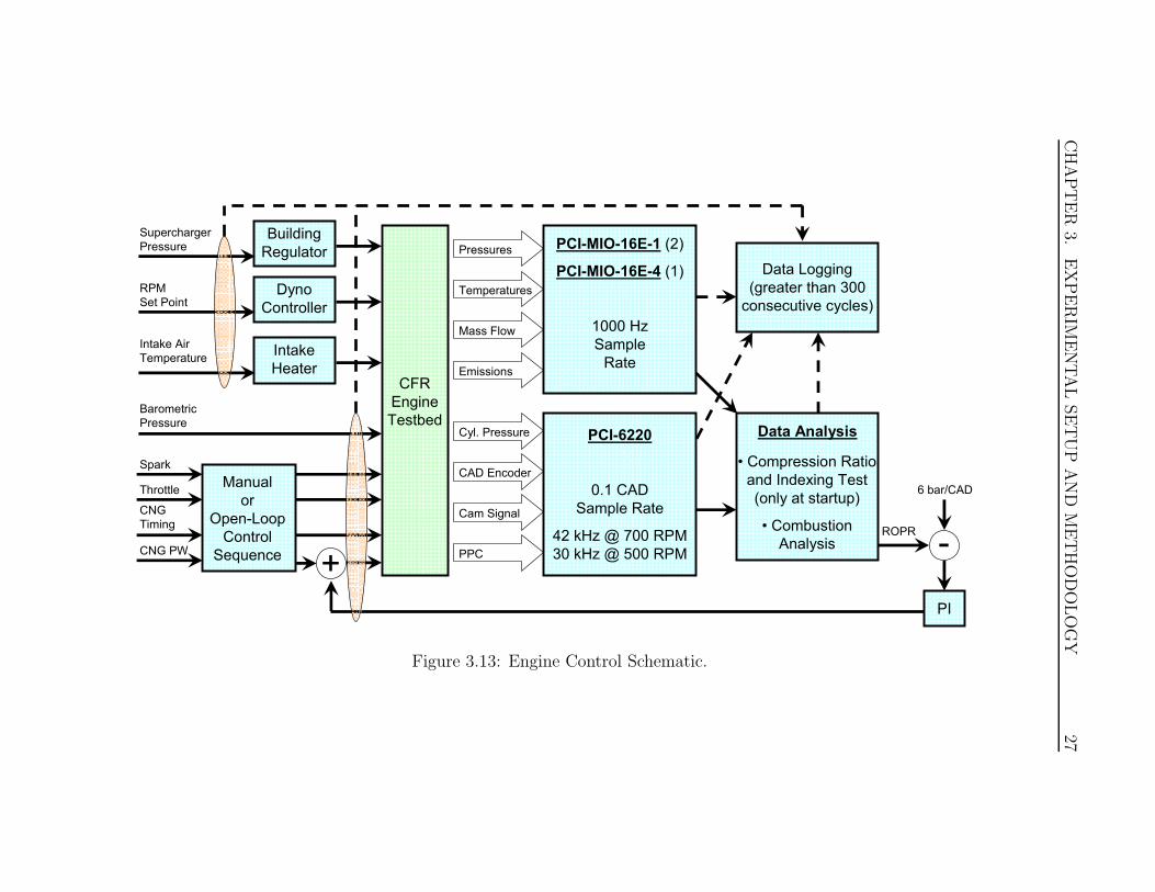
3.2 Engine Data-Logging/Analysis/Control Program
To carry out transient tests for mode-switching, a suitable control program is nec-
essary. Using previous software from Handford and Hosseini as a basis [16, 19], an
enhanced control program is developed to meet the following requirements: cycle-
based synchronization; data collection from all sensors with on-line analysis to
evaluate combustion; feedback capability using calculated parameters; open-loop
control of actuators; and data logging of all measurements and calculations. Pro-
gram operation is summarized in Figure 3.13.
The program is run on a single desktop PC operating with a Pentium IV 2.4
GHz dual-core processor and 2 GB of RAM. The Windows XP operating system
is used along with LabVIEW version 7.1.1. All data-acquisition and control is
carried out directly from the host PC. Details regarding channel configuration and
program functionality can be found in Appendix F.
CHAPTER
3.EXPERIM
ENTALSETUP
AND
METHODOLOGY
27
Pressures
Temperatures
Mass Flow
Emissions
Cyl. Pressure
PPC
Cam Signal
PCI-MIO-16E-1 (2)
PCI-MIO-16E-4 (1)
1000 Hz
Sample
Rate
PCI-6220
0.1 CAD
Sample Rate
42 kHz @ 700 RPM
30 kHz @ 500 RPM
CFR
Engine
Testbed
CAD Encoder
Data Logging
(greater than 300
consecutive cycles)
• Compression Ratio
and Indexing Test
(only at startup)
• Combustion
AnalysisROPR
6 bar/CAD
-
PI
+
Throttle
Dyno
Controller
RPM
Set Point
Intake
Heater
Intake Air
Temperature
Building
Regulator
Supercharger
Pressure
Manual
or
Open-Loop
Control
SequenceCNG PW
CNG
Timing
Spark
Barometric
PressureData Analysis
Figure 3.13: Engine Control Schematic.
CHAPTER 3. EXPERIMENTAL SETUP AND METHODOLOGY 28
3.2.1 Injection Timing Limitation
Calculations for evaluating combustion parameters initiate at a common point dur-
ing the exhaust stroke on every cycle. As the system is busy and an external pro-
cessor is not used, injection is not possible during this time. The affected region
extends from 190◦ bIVO to approximately 40◦ bIVO at 700 RPM. As engine speed
increases, the calculation time of approximately 14 ms remains unchanged, but the
crank angle at which it finishes approaches IVO. To ensure sufficient calculation
time and allow for variability, injection timing is restricted to IVO as the earliest
point after the calculation period. Injection during the intake stroke is avoided
so all CNG is inducted on a single engine cycle and not partially trapped in the
intake manifold. Delaying the injection until after IVC incurs a one-cycle delay
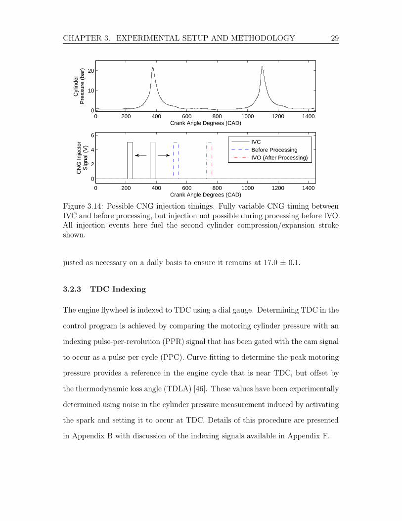
in fuel delivery. Figure 3.14 summarizes the possible injection timings considering
these limitations. The labeled events indicate the limiting cases, while the timing
is variable between IVO and the start of processing. Further details pertaining to
fuel injection can be found in Appendix F.
3.2.2 Effective Compression Ratio
Compression ratio has a strong effect on combustion and is necessary to evaluate
certain combustion parameters. Due to the optical head installed on the CFR
engine and the high compression ratios necessary for natural gas HCCI, clearance
volume can not be directly measured to determine compression ratio. A means of
evaluating the effective compression ratio by comparing peak motored pressure to
values obtained from a single zone chemical kinetic model using air as the working
fluid was implemented previously [16,19]. Using a similar approach but augmenting
intake pressure improves the repeatability despite atmospheric pressure changes.
Details are provided in Appendix A.
Compression ratio is not varied throughout this study, but is checked and ad-
CHAPTER 3. EXPERIMENTAL SETUP AND METHODOLOGY 29
0 200 400 600 800 1000 1200 14000
10
20
Crank Angle Degrees (CAD)
Cyl
inde
rP
ress
ure
(bar
)
0 200 400 600 800 1000 1200 1400
0
2
4
6
Crank Angle Degrees (CAD)
CN
G In
ject
orS
igna
l (V
)
IVCBefore ProcessingIVO (After Processing)
Figure 3.14: Possible CNG injection timings. Fully variable CNG timing betweenIVC and before processing, but injection not possible during processing before IVO.All injection events here fuel the second cylinder compression/expansion strokeshown.
justed as necessary on a daily basis to ensure it remains at 17.0 ± 0.1.
3.2.3 TDC Indexing
The engine flywheel is indexed to TDC using a dial gauge. Determining TDC in the
control program is achieved by comparing the motoring cylinder pressure with an
indexing pulse-per-revolution (PPR) signal that has been gated with the cam signal
to occur as a pulse-per-cycle (PPC). Curve fitting to determine the peak motoring
pressure provides a reference in the engine cycle that is near TDC, but offset by
the thermodynamic loss angle (TDLA) [46]. These values have been experimentally
determined using noise in the cylinder pressure measurement induced by activating
the spark and setting it to occur at TDC. Details of this procedure are presented
in Appendix B with discussion of the indexing signals available in Appendix F.
CHAPTER 3. EXPERIMENTAL SETUP AND METHODOLOGY 30
3.3 Combustion Analysis
Combustion timing (CA50), severity (maximum rate of pressure rise, ROPR), and
power level (IMEP) are evaluated using the in-cylinder pressure trace, which is
sampled at 0.1 CAD. Operating stability is characterized by variation in IMEP
(COV IMEP). These parameters are computed using the same methodology as
Handford [19] with the exception of a different heat transfer correlation during
SI operation for CA50. Detailed error analysis is carried out in Appendix E with
a summary provided in Section 3.5 below.
3.3.1 CA50
Combustion timing is represented by the point at which 50% of the fuel has been
burned (CA50). Values are presented as crank angle degrees after TDC on the
compression stroke (◦aTDC). Gross heat release is calculated by adding the calcu-
lated net heat release [47] to the heat loss. Since mode-switching between SI and
HCCI is the focus of this study, different heat loss correlations are implemented for
each mode. SI heat loss is evaluated using the traditional Woschni correlation [48],
while a modified Woschni correlation [7] is used for HCCI operation similar to
Handford [19]. The appropriate set of parameters is selected based on whether the
spark is activated (SI) or not (HCCI).
The effect of CA50 being determined for HCCI combustion but using the SI
heat loss relation results in the timing being retarded past the expected value by
approximately 5◦ as shown in Table E.1. During mode-switching, the spark may
remain activated for a few cycles where HCCI combustion is clearly evident in the
cylinder pressure traces.
During misfire or partial combustion cycles, sufficient heat release may not be
available to compute CA50 properly. These cycles are assigned a value of -60◦
aTDC for CA50. In data figures, these points fall below the displayed axis range
CHAPTER 3. EXPERIMENTAL SETUP AND METHODOLOGY 31
to improve readability of actual CA50 data.
3.3.2 IMEP
Engine power output is evaluated using indicated mean effective pressure (IMEP),
which is calculated by integrating the cylinder pressure with respect to volume
throughout an engine cycle, then dividing by the displacement volume [1]. This
method of representing engine power neglects friction losses that are typically much
higher in the CFR engine compared to a modern engine.
Discrete cylinder pressure measurements at 0.1 CAD resolution are made in
this study, so IMEP is evaluated using
IMEP =
7200∑
i=1
Pi dVi
Vd
(3.5)
where Pi is the cylinder pressure at each measurement and Vd is the displacement
volume. The change in volume over each 0.1 CAD increment (dVi) is calculated
with the slider-crank relation
V = Vc +π B2
4(l + a− a cosθ −
√l2 − a2 sin2θ) (3.6)
where V is the cylinder volume for a given angular crank position past TDC (θ), B
is the cylinder bore, l is the connecting rod length, and a is the crank swing (half
of the stroke). The clearance volume (Vc) is calculated using
Vc =Vd
rc − 1(3.7)
where rc is the compression ratio.
CHAPTER 3. EXPERIMENTAL SETUP AND METHODOLOGY 32
3.3.3 COV IMEP
Stability of the engine is determined by observing the coefficient of variation among
calculated IMEP values (COV IMEP). This is done by dividing the standard devi-
ation of a certain number of IMEP (σIMEP) cycles by the mean IMEP (µIMEP) as
shown
COV IMEP =σIMEP
µIMEP(3.8)
A total of 450 cycles are used to determine COV IMEP for each steady-state operat-
ing point. Stable combustion is commonly limited at a COV IMEP of 5% for modern
engines [20,21,32]; however, a value of 10% is adoped in this study as is typical for
research using CFR engines [19, 49].
3.3.4 Maximum Rate of Pressure Rise (ROPR)
Combustion severity or harshness is evaluated using the maximum rate of pressure
rise (ROPR) of cylinder pressure. The cylinder pressure trace is first filtered us-
ing a low-pass butterworth filter (bidirectional 3rd order with normalized cutoff
frequency of 0.10) to remove noise that may otherwise overestimate the degree of
harshness, then the point of maximum slope is determined as
ROPR =
(
dP cyl
dθ
)
max
(3.9)
Cycles with ROPR greater than 10 bar/CAD are considered knock as in previous
studies [19, 49] and avoided where possible during mode-switching.
3.4 Test Procedure
Prior to starting the engine, the atmospheric pressure in the lab is measured using
a mercury barometer and entered as an input to the control program. The engine
CHAPTER 3. EXPERIMENTAL SETUP AND METHODOLOGY 33
is motored at an intake pressure of 65 kPa, spark is activated at 5◦ aTDC, and
fuel is injected at IVC to achieve stoichiometric combustion before switching the
dynomometer to “absorb” mode. After running at 700 RPM until coolant temper-
ature reaches steady-state of approximately 98 ◦C, fuel is turned off and the motor
coasts to a stop. The engine is motored again at 1000 RPM with wide open throttle
for 5 minutes to allow stabilization of coolant and cylinder wall temperatures. A
compression ratio test is completed to measure compression ratio, rising cam edge
location, and peak pressure location. Thermodynamic loss angle (see Appendix
B) is automatically added to the peak pressure location based on the measured
compression ratio to index the location of geometric TDC relative to the pulse per
cycle (PPC) signal.
The engine is now ready to begin testing. First, the desired operating point
must be achieved. Throttle and fuel are adjusted to initiate SI combustion and
the dynomometer is again switched to “absorb” mode. RPM is set at the desired
level, the intake heater activated, and building air regulator opened to supercharge
the intake system. The engine is allowed to stabilize until mixture temperature
(Tmix) remains within a ± 2 ◦C tolerance before open-loop mode-switching tests
are initiated.
When running a mode-switch test, the intake air temperature controller is al-
lowed to stabilize within 1 ◦C of set point before initiating data collection. After
approximately 50 cycles in the initial combustion mode, the open-loop sequence is
activated and the engine transitions to the other combustion mode. Data collec-
tion continues for a total of 300 cycles to capture the response from the emissions
bench.
CHAPTER 3. EXPERIMENTAL SETUP AND METHODOLOGY 34
3.5 Mode-Switching Data Plots - Description and Uncertainties
To represent the repeatability of mode-switching strategies during development, a
set of 10 tests are carried out for each open-loop control strategy. Plotting data
individually for each test makes comparisons difficult. A method is developed to
display all representative data in three figures per set of tests to simplify analysis.
The first figure contains all control inputs during the mode-switch and the
IMEP response. Controls include intake pressure as adjusted by throttle position,
CNG injector pulse width, and CNG injection timing for some tests. The second
figure provides cylinder pressure traces immediately surrounding the mode-switch
cycle to show combustion characteristics. The third figure presents the calculated
combustion parameters CA50 and ROPR.
One test for each set of 10 is selected and displayed as an example with charac-
teristics that best describe engine behavior. In order to display all 10 tests, shaded
regions are used. A lighter colored region displays extremum of the 10 data sets
at each cycle. The inner darker colored region displays the range of the 6 values of
the data set at each cycle. The standard deviation is not used since the data are
not always normally distributed. Using these two regions, visual inspection can
be used to determine whether certain deviations are common or occur less than 2
times out of 10 tests. Error bars presented in these figures are not easily visible,
so Table 3.4 lists the error for individual parameters as determined in Appendices
D and E.
3.6 Mode-Switching Evaluation
Mode-switching is typically evaluated using a qualitative analysis labeling a transi-
tion by varying degrees of “smooth” and “quick”. The definition of these descriptors
varies among researchers, making it difficult to compare various methods of induc-

CHAPTER 3. EXPERIMENTAL SETUP AND METHODOLOGY 35
Table 3.4: Measurement uncertainty at 95% confidence for values presented inmode-switching data plots.
Parameter Symbol UncertaintyAverage Intake Pressure εIntakePressure 2.7 kPaP IVC εPIV C 2.8 kPaCNG PW - -CNG Timing εCNGTiming 1.1 CADIMEP εIMEP 0.06 barCA50 (SI/HCCI) εCA50 3.1/0.89 CADROPR εROPR 0.03 bar/CADEquivalence Ratio εEquivalenceRatio 12%
ing a mode-switch in an engine. A quantitative evaluation of these conditions is
needed to provide comparisons between methods as well as a means of optimizing
a mode-switch through a tuning process.
Conditions requiring consideration include duration of the transition, IMEP dur-
ing the transition, and undesirable combustion including knock and misfire cycles.
A quantitative evaluation should include a means of monitoring these events and
reflect their influence on the overall performance of the mode-switch. Combining
these parameters with suitable weighting factors allows for a single mode-switching
performance criterion (MSPC) to quantify the performance of the mode-switch,
with lower values indicating better mode-switch performance. The MATLAB code
developed for this analysis is included in Appendix G.
3.6.1 Duration
The number of cycles required to complete a mode-switch must be defined. The
combustion occurring during the period between stable operation in SI and HCCI
may consist of hybrid cycles showing characteristic of both forms of combustion.
This is interesting from a research standpoint, but the desirable parameter to mon-
itor is the power developed during these transitional cycles. IMEP should, in the
ideal case, step from the steady-state level in the initial mode of operation to
CHAPTER 3. EXPERIMENTAL SETUP AND METHODOLOGY 36
the desired steady-state level in the target combustion mode and remain constant
thereafter until controlled otherwise. This definition covers all possible mode-switch
scenarios, including a step up in power, a step down in power, or maintaining a
given power level.
The start of the mode-switch is easily defined as the first cycle after the switch
has been commanded by the control system. This is indicated by a change in any
actuator from its initial state of stable operation.
Difficulty arises in deciding when the engine shall be considered stable at the
new IMEP under the different form of combustion. Because COV IMEP is a common
measure for combustion stability, this value should suitably define this condition.
By calculating a running value of COV IMEP, the point at which this value drops
below some threshold is considered the last cycle of the mode-switch. A COV IMEP
of 5% is commonly associtated with the maximum variablilty in IMEP suitable for
stable performance, and is adopted as the threshold for this criterion. An exception
exists when the state being transitioned into carries a higher steady-state COV IMEP
than 5%, suggesting that the mode-switch will never be considered complete based
on this criteria. For this study, only Section 4.5 falls into this category, where
operation in SI carries a COV IMEP of 11%, dictating the minimum threshold to
define the end of the mode-switch.
The number of cycles used to evaluate COV IMEP is determined from early test-
ing. Figures 4.2, 4.6, and 4.10 show a typical transition period of 15 cycles between
steady-state IMEP in SI and HCCI combustion modes. This is selected as a suit-
able period over which to calculate COV IMEP to determine whether the engine has
achieved steady-state operation. Smaller numbers of cycles increase the sensitiv-
ity of COV IMEP toward variability that may include normal operation in the final
state, while larger numbers may predict the mode-switch to be complete sooner
than is reasonable. The procedure used to determine duration of the mode-switch
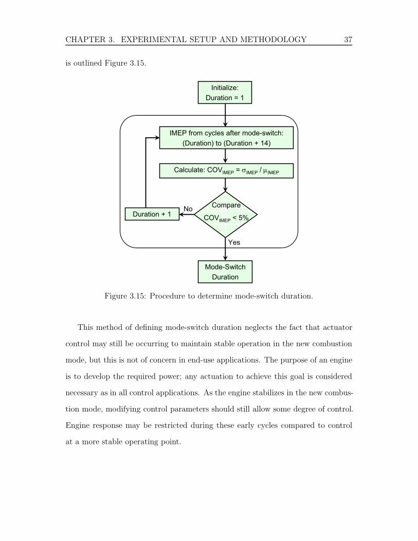
CHAPTER 3. EXPERIMENTAL SETUP AND METHODOLOGY 37
is outlined Figure 3.15.
Initialize:
Duration = 1
IMEP from cycles after mode-switch:
(Duration) to (Duration + 14)
Calculate: COVIMEP = σIMEP / µIMEP
Duration + 1
Compare
COVIMEP < 5%
Mode-Switch
Duration
No
Yes
Figure 3.15: Procedure to determine mode-switch duration.
This method of defining mode-switch duration neglects the fact that actuator
control may still be occurring to maintain stable operation in the new combustion
mode, but this is not of concern in end-use applications. The purpose of an engine
is to develop the required power; any actuation to achieve this goal is considered
necessary as in all control applications. As the engine stabilizes in the new combus-
tion mode, modifying control parameters should still allow some degree of control.
Engine response may be restricted during these early cycles compared to control
at a more stable operating point.

CHAPTER 3. EXPERIMENTAL SETUP AND METHODOLOGY 38
3.6.2 Smoothness
Similar to steady-state operation, it is desirable to minimize variability of IMEP
from the desired trend throughout a mode-switch. These target values must be de-
fined for a variable number of cycles as determined by the duration above. Steady-
state values for IMEP in both the initial and final combustion modes can be evalu-
ated as the average of the same 15 engine cycles for which COV IMEP is calculated.
For the intermediate cycles during the mode-switch, a linear progression is chosen
to represent the smoothest transition.
Comparing experimental IMEP to this target trend, a transient form of COV IMEP
is calculated. Instead of computing standard deviation with an average IMEP, the
residuals are considered for each cycle throughout the duration using
σIMEP trans =
√
√
√
√
1
Duration
Duration∑
i=1
(IMEP actual − IMEP target)2 (3.10)
Mean IMEP for the mode-switch (µIMEP trans) is the average between the initial
and final states
µIMEP trans =IMEP initial + IMEP final
2(3.11)
Finally, COV IMEP trans is evaluated as
COV IMEP trans =σIMEP trans
µIMEP trans(3.12)
3.6.3 Knock
High rates of pressure rise lead to harsh combustion having several drawbacks.
Advanced combustion timing is typically associated with knock in HCCI and may
lead to less efficient operation, significantly increased NOx emissions, higher peak
pressures, audible noise, and potential engine damage.
CHAPTER 3. EXPERIMENTAL SETUP AND METHODOLOGY 39
Similar to steady-state operation, ROPR is used to detect knock. Any cycles
producing ROPR greater than 10 bar/CAD are considered knock cycles. A penalty
is applied for each of these cycles during the mode-switch thereafter until knock
propagation has ceased. The end of this stabilization period is determined, similar
to the duration parameter, through a 15 cycle running check for knock.
3.6.4 Misfire
Misfire cycles occur when the air/fuel mixture does not ignite. This results in a
negative IMEP value and a significant disturbance in power output and emissions.
Partial burn cycles are also of concern in HCCI where only a portion of the fuel
energy is released, leaving a large portion unburned with the associated reduction
in power delivery. Both of these conditions will influence the smoothness parameter
as described above, but a further penalty may also be deemed necessary.
3.6.5 Weighting Factors
Combining the above factors into a single value to describe mode-switch perfor-
mance introduces the possibility of weighting the components differently. Duration
is chosen as the basis with each cycle during the transition carrying a weight of 1.
Smoothness is calculated similar to steady-state operation where a commonly
accepted COV IMEP of 5% dictates the stability limit. As such, COV IMEP trans can
be normalized around 5% with any value greater than 1 incurring a penalty. A
weighting of half the duration is found to correlate with qualitative evaluation and
provide a duration-sensative component for proportional penalties.
Knock is considered when ROPR exceeds the threshold value of 10 bar/CAD,
with any offending cycles incurring a penalty. Since knock is associated with po-
tential engine damage, a more severe penalty is necessary. The degree of knock
is taken into account by applying a linear penalty of 1 for every 2 bar/CAD over

CHAPTER 3. EXPERIMENTAL SETUP AND METHODOLOGY 40
the threshold at each knock cycle. This weighting is not dependent on duration as
knock is event specific and not a relative measure such as smoothness.
Misfire cycles already carry a heavy penalty based on the smoothness crite-
ria, with partial burn cycles incurring a proportionally smaller impact. A further
penalty for misfire cycles is deemed unnecessary at this point.
All conditions are combined to determine the MSPC using
MSPC =
Duration
+Duration
2
(
COV IMEP trans
0.05− 1
)
COV IMEP trans > 0.05
+1
2
(
Stabilize∑
i=1
ROPRi − 10
)
ROPRi > 10
(3.13)
The weight factors being applied here may be considered to be application spe-
cific; however, this may not be the case. For example, large industrial engines
with high flywheel mass are less sensitive to IMEP variability than small automo-
tive engines. These two applications also require different levels of response time,
with smaller automotive-type engines being required to reach the new operating
mode and desired power output much more quickly than heavy industrial engines.
Knock follows the same trend with industrial engines being less prone to damage
than smaller engines. With all conditions having more stringent requirements for
automotive in comparison to industrial engines, this suggests that the needs of
different applications may be met by specifying a different minimal level of MSPC
to design toward as opposed to shifting the weighting factors.
41
Chapter 4
SI-HCCI-SI Mode-Switch Results
The primary objective of mode-switching is to transition between combustion
modes. This chapter focuses on developing an open-loop strategy to transition
between SI and HCCI at 700 RPM in a smooth and quick manner using only
conventional actuators: throttle, CNG injection pulse width, and CNG injection
timing. The mode-switching performance criterion (MSPC) described in Chapter
3 is used to highlight areas where attention is necessary for improvement. After op-
timizing the control strategy based on MSPC to a one-cycle step in IMEP between
combustion modes, stability is evaluated by quickly repeating mode-switches. Flex-
ibility is explored by profiling various levels of IMEP before/after the mode-switch
at a slower engine speed of 500 RPM.
4.1 Steady-State Operating Conditions - Large Manifold
To examine mode-switching, compatible SI and HCCI steady-state operating points
are found. The requirement for compatibility is that parameters such as intake
temperature that can not be changed quickly must be similar for both modes. It can
be difficult to find compatible points since a high intake temperature leads to knock
in SI while a low intake temperature may result in HCCI ignition not occurring.
Two operating points, shown in Table 4.1, are one example of compatible points
CHAPTER 4. SI-HCCI-SI MODE-SWITCH RESULTS 42
that will be used for testing with the large intake manifold.
Intake pressures are chosen based on a throttling limitation in SI for the super-
charger pressure required for HCCI operation. Throttle openings greater than 33%
have little influence on intake pressure due to the large intake manifold volume and
are avoided to simplify control.
Late spark timing of 5◦ aTDC is required in SI mode since the intake tempera-
ture is high (115 ◦C). This leads to late combustion timing of CA50 = 48◦ aTDC.
Stability in SI mode is poor as indicated by the COV IMEP of 11% slightly above the
misfire limit of 10%. To allow HCCI operation at the same intake air temperature,
the combustion instability of 11 % is accepted as a compromise.
Operating in HCCI at this point is also not highly stable due to the low in-
take temperature. With CNG pulse width (CNG PW) set to the value shown, the
engine may eventually misfire or knock after a period of time. A manually tuned
PI controller applies adjustments to the nominal CNG PW to maintain ROPR
at 6 bar/CAD. Slow response is attained through gains of 0.120 for proportional
and 0.050 for integral, while variability in HCCI combustion is handled by aver-
aging ROPR over 5 previous cycles for the reference value. These settings remain
unchanged throughout testing.
4.2 SI-HCCI: Intake Pressure - Step Increase
Achieving the new steady-state conditions as quickly as possible using open-loop
tuning of CNG amount and throttle position is the first mode-switch strategy.
The throttle is opened over 3 cycles for a compromise between intake pressure
response time and overshoot, while CNG delivery is adjusted to maintain suitable
combustion throughout the transition. The sequence of fuel values is developed by
iteration through repeated switching and manual tuning. Fuel delivery is initially
set low on each cycle to induce misfire rather than knock, with successive tests
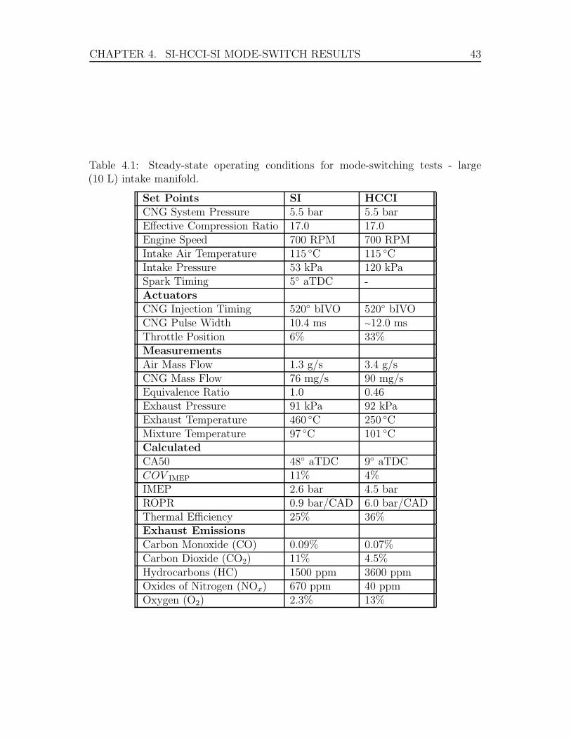
CHAPTER 4. SI-HCCI-SI MODE-SWITCH RESULTS 43
Table 4.1: Steady-state operating conditions for mode-switching tests - large(10 L) intake manifold.
Set Points SI HCCICNG System Pressure 5.5 bar 5.5 barEffective Compression Ratio 17.0 17.0Engine Speed 700 RPM 700 RPMIntake Air Temperature 115 ◦C 115 ◦CIntake Pressure 53 kPa 120 kPaSpark Timing 5◦ aTDC -ActuatorsCNG Injection Timing 520◦ bIVO 520◦ bIVOCNG Pulse Width 10.4 ms ∼12.0 msThrottle Position 6% 33%MeasurementsAir Mass Flow 1.3 g/s 3.4 g/sCNG Mass Flow 76 mg/s 90 mg/sEquivalence Ratio 1.0 0.46Exhaust Pressure 91 kPa 92 kPaExhaust Temperature 460 ◦C 250 ◦CMixture Temperature 97 ◦C 101 ◦CCalculatedCA50 48◦ aTDC 9◦ aTDCCOV IMEP 11% 4%IMEP 2.6 bar 4.5 barROPR 0.9 bar/CAD 6.0 bar/CADThermal Efficiency 25% 36%Exhaust EmissionsCarbon Monoxide (CO) 0.09% 0.07%Carbon Dioxide (CO2) 11% 4.5%Hydrocarbons (HC) 1500 ppm 3600 ppmOxides of Nitrogen (NOx) 670 ppm 40 ppmOxygen (O2) 2.3% 13%
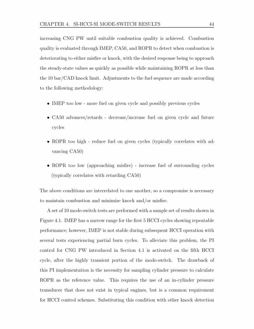
CHAPTER 4. SI-HCCI-SI MODE-SWITCH RESULTS 44
increasing CNG PW until suitable combustion quality is achieved. Combustion
quality is evaluated through IMEP, CA50, and ROPR to detect when combustion is
deteriorating to either misfire or knock, with the desired response being to approach
the steady-state values as quickly as possible while maintaining ROPR at less than
the 10 bar/CAD knock limit. Adjustments to the fuel sequence are made according
to the following methodology:� IMEP too low - more fuel on given cycle and possibly previous cycles� CA50 advances/retards - decrease/increase fuel on given cycle and future
cycles� ROPR too high - reduce fuel on given cycles (typically correlates with ad-
vancing CA50)� ROPR too low (approaching misfire) - increase fuel of surrounding cycles
(typically correlates with retarding CA50)
The above conditions are interrelated to one another, so a compromise is necessary
to maintain combustion and minimize knock and/or misfire.
A set of 10 mode-switch tests are performed with a sample set of results shown in
Figure 4.1. IMEP has a narrow range for the first 5 HCCI cycles showing repeatable
performance; however, IMEP is not stable during subsequent HCCI operation with
several tests experiencing partial burn cycles. To alleviate this problem, the PI
control for CNG PW introduced in Section 4.1 is activated on the fifth HCCI
cycle, after the highly transient portion of the mode-switch. The drawback of
this PI implementation is the necessity for sampling cylinder pressure to calculate
ROPR as the reference value. This requires the use of an in-cylinder pressure
transducer that does not exist in typical engines, but is a common requirement
for HCCI control schemes. Substituting this condition with other knock detection
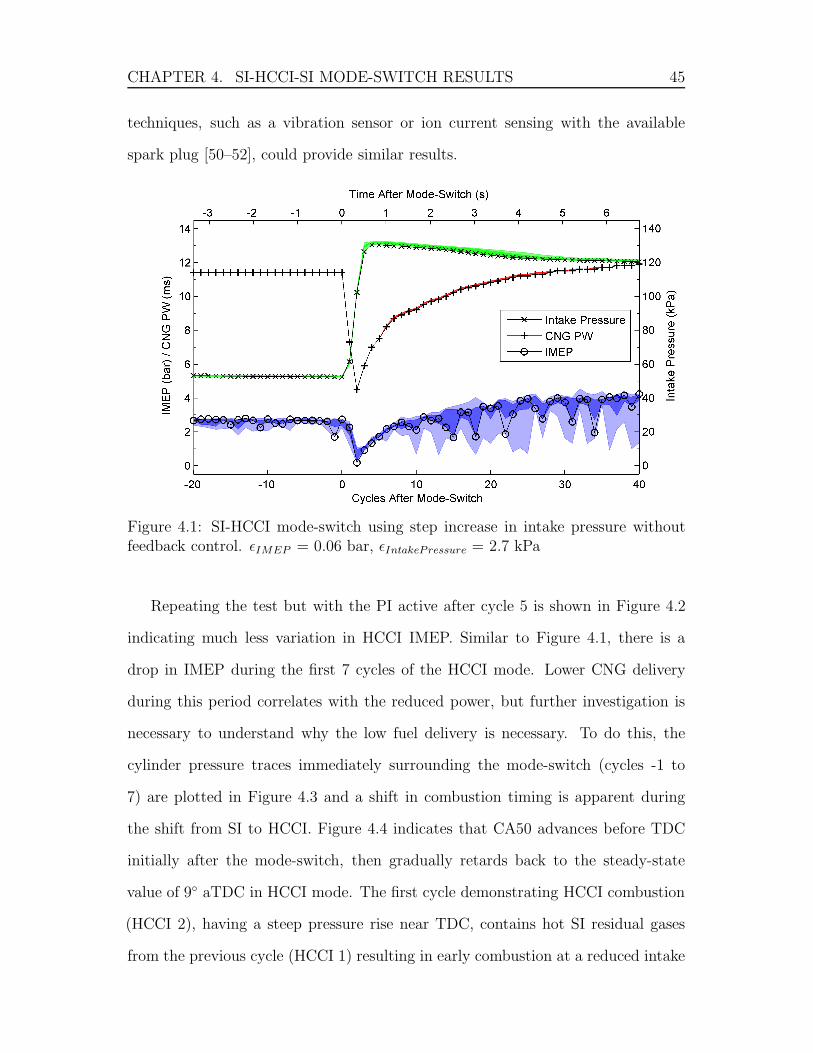
CHAPTER 4. SI-HCCI-SI MODE-SWITCH RESULTS 45
techniques, such as a vibration sensor or ion current sensing with the available
spark plug [50–52], could provide similar results.
Figure 4.1: SI-HCCI mode-switch using step increase in intake pressure withoutfeedback control. εIMEP = 0.06 bar, εIntakePressure = 2.7 kPa
Repeating the test but with the PI active after cycle 5 is shown in Figure 4.2
indicating much less variation in HCCI IMEP. Similar to Figure 4.1, there is a
drop in IMEP during the first 7 cycles of the HCCI mode. Lower CNG delivery
during this period correlates with the reduced power, but further investigation is
necessary to understand why the low fuel delivery is necessary. To do this, the
cylinder pressure traces immediately surrounding the mode-switch (cycles -1 to
7) are plotted in Figure 4.3 and a shift in combustion timing is apparent during
the shift from SI to HCCI. Figure 4.4 indicates that CA50 advances before TDC
initially after the mode-switch, then gradually retards back to the steady-state
value of 9◦ aTDC in HCCI mode. The first cycle demonstrating HCCI combustion
(HCCI 2), having a steep pressure rise near TDC, contains hot SI residual gases
from the previous cycle (HCCI 1) resulting in early combustion at a reduced intake

CHAPTER 4. SI-HCCI-SI MODE-SWITCH RESULTS 46
pressure compared to steady-state [41]. Subsequent HCCI cycles have an intake
pressure slightly above the desired intake pressure of 120 kPa and have HCCI
residuals present, yet continue to produce early combustion timing with very lean
mixtures. ROPR is maintained below the knock limit of 10 bar/CAD (except for
a few occurrences near cycle 25 and 35) with the low CNG PW shown in Figure
4.2, but at the expense of reduced IMEP. This behavior is attributed to the hot
combustion chamber surfaces and a hot exhaust valve (from SI mode) promoting
early ignition [24,40]. This advanced combustion following a mode-switch from SI
to HCCI needs to be counteracted in future tests to achieve a smoother transition
and will be considered in the next section.
Figure 4.2: SI-HCCI mode-switch using step increase in intake pressure with PIcontrol of fuel activated after 5 HCCI cycles1. εIMEP = 0.06 bar, εIntakePressure =2.7 kPa
1CNG PW during steady-state SI operation is 11.4 ms instead of 10.4 ms as in other testswith the large manifold. Rich operation is confirmed by increased levels of HC and CO in theexhaust measurements. This setting was chosen to achieve a stoichiometric mixture based on themass flow rates of CNG and air. Calibration error and/or variation in CNG composition [53] arepotential causes for this discrepancy.
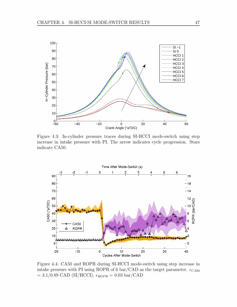
CHAPTER 4. SI-HCCI-SI MODE-SWITCH RESULTS 47
−60 −40 −20 0 20 40 600
10
20
30
40
50
60
70
80
90
100
Crank Angle (°aTDC)
In−
Cyl
inde
r P
ress
ure
(bar
)
SI −1SI 0HCCI 1HCCI 2HCCI 3HCCI 4HCCI 5HCCI 6HCCI 7
Figure 4.3: In-cylinder pressure traces during SI-HCCI mode-switch using stepincrease in intake pressure with PI. The arrow indicates cycle progression. Starsindicate CA50.
Figure 4.4: CA50 and ROPR during SI-HCCI mode-switch using step increase inintake pressure with PI using ROPR of 6 bar/CAD as the target parameter. εCA50
= 3.1/0.89 CAD (SI/HCCI), εROPR = 0.03 bar/CAD

CHAPTER 4. SI-HCCI-SI MODE-SWITCH RESULTS 48
Mode-switching effectiveness is evaluated using the MSPC outlined in Chapter
3. Individual IMEP data for each of the 10 tests is provided in Figure 4.5 along
with the calculated MSPC components in Table 4.2. These results support the ob-
servable performance discussed above, with the drop in IMEP during early HCCI
operation causing a significant penalty in the smoothness value (higher values in-
dicate less desirable mode-switch performance).

CHAPTER 4. SI-HCCI-SI MODE-SWITCH RESULTS 49
−10 0 10 20 300
2
4
6
Cycles After Mode Switch
IME
P (
bar)
2010_03_17 − 17
−10 0 10 20 300
2
4
6
Cycles After Mode Switch
IME
P (
bar)
2010_03_17 − 18
−10 0 10 20 300
2
4
6
Cycles After Mode Switch
IME
P (
bar)
2010_03_17 − 19
−10 0 10 200
2
4
6
Cycles After Mode SwitchIM
EP
(ba
r)
2010_03_17 − 20
−10 0 10 20 300
2
4
6
Cycles After Mode Switch
IME
P (
bar)
2010_03_17 − 21
−10 0 10 20 300
2
4
6
Cycles After Mode Switch
IME
P (
bar)
2010_03_17 − 22
−10 0 10 20 300
2
4
6
Cycles After Mode Switch
IME
P (
bar)
2010_03_17 − 23
−10 0 10 20 30 400
2
4
6
Cycles After Mode Switch
IME
P (
bar)
2010_03_17 − 24
−10 0 10 20 300
2
4
6
Cycles After Mode Switch
IME
P (
bar)
2010_03_17 − 25
−10 0 10 20 300
2
4
6
Cycles After Mode Switch
IME
P (
bar)
2010_03_17 − 27
Figure 4.5: IMEP data from Section 4.2 to evaluate smoothness for MSPC. Exper-imental data sets are shown with the desired trend.

CHAPTER
4.SI-H
CCI-S
IMODE-SW
ITCH
RESULTS
50
Table 4.2: MSPC data for Section 4.2.
Test Date Test Number Standard
2010 03 17 17 18 19 20 21 22 23 24 25 27 Average Deviation
Duration 16 19 16 15 18 16 22 34 23 20 19.90 5.65
Smoothness 40.80 40.17 33.40 35.89 49.08 38.45 38.48 45.62 43.38 37.75 40.30 4.66
Stabilize 16 19 16 15 18 26 22 34 23 20 20.90 5.76
Knock 0.00 0.00 0.00 0.00 0.00 1.01 0.00 0.00 0.00 0.00 0.10 0.32
MSPC 56.80 59.17 49.40 50.89 67.08 55.46 60.48 79.62 66.38 57.75 60.30 8.86

CHAPTER 4. SI-HCCI-SI MODE-SWITCH RESULTS 51
4.3 SI-HCCI: Intake Pressure - First-Order Increase
A method to avoid HCCI cycles having combustion timing that are too advanced
(CA50 bTDC) immediately following an SI/HCCI mode-switch is investigated. One
approach to retard HCCI combustion timing is to reduce compression temperatures,
thus delaying the point where auto-ignition conditions are achieved. Lower intake
pressure reduces the total mass of gases inducted into the engine equating to lower
compression temperatures. To implement this on the engine, intake pressure is
increased at a slower rate than the previous test and the fuel sequence is determined
using the same criteria. To constrain the number of variables for manual tuning, the
intake pressure is increased at a rate dictated by a step increase in throttle position.
The large intake manifold produces a first-order increase in intake pressure with a
time constant that varies with the magnitude of step in throttle position.
The timing of the throttle step with respect to the mode-switch is now an
added parameter that must be determined. In the previous test, the large increase
of intake pressure between two cycles provided a trigger to switch to HCCI. In this
case with a slower pressure rise, however, no such trigger exists. If the switch is
made too early, then subsequent HCCI cycles are highly sensitive to intake pressure
and CNG PW, and not easily maintained between misfire and knock with open loop
control. If the mode-switch is delayed too long after the throttle step, then knock
may occur. Through testing, it is found that inducing HCCI combustion on the
fourth cycle after initiating the mode-switch provides the smoothest transition with
open-loop control.
Deciding on the fuel delivery during the initial 5 cycles after the throttle step is
more difficult than in the previous test since these cycles fall outside normal SI and
HCCI operating regions and neither mode of combustion is stable. An approach of
supplying progressively leaner mixtures is implemented to gradually promote HCCI
combustion by reducing the cooling effect of room temperature CNG injected into
CHAPTER 4. SI-HCCI-SI MODE-SWITCH RESULTS 52
the hot intake air. The natural tendency toward advanced combustion found in
Section 4.2 should be beneficial in this scenario by promoting HCCI ignition during
these unstable cycles. The spark remains on during the initial 5 cycles after the
throttle step to further promote ignition.
Figure 4.6 shows that this strategy with a slower intake pressure rise presents
an improvement over the previous tests in Section 4.2 as the drop in IMEP is
removed. Higher combustion variability in CA50 is apparent during the first few
cycles, particularly cycle 3 after mode-switch. Figure 4.7 confirms this with combus-
tion occurring late in SI mode for the first 2 cycles and little apparent combustion
in the third cycle. Starting with the fourth cycle, HCCI combustion occurs with
late CA50 timing. CA50 and ROPR shown in Figure 4.8 support this observation
with CA50 quickly advancing on the third cycle and ROPR increasing thereafter -
note that the step in CA50 between cycles 5 and 6 after mode-switch is attributed
to a change in Woschni coefficients as the spark is turned off.
High sensitivity to the amount of fuel delivered each cycle is experienced using
this method, making it difficult to develop an open-loop sequence. Combustion
during the unstable cycles early in the mode-switch sometimes produce misfires
while other cycles ignite normally or even knock slightly. As is visible in the CNG
PW values at cycles 2-3, adaptive adjustment is necessary during the 10 tests since
in consecutive tests combustion deteriorated on the third cycle.
HCCI combustion is influenced by previous cycles through the exhaust residual
and this coupling of cycles can lead to unstable combustion dynamics. For example,
some tests progress to knock while others transition to late combustion timing and
misfire.
With the reduction in IMEP removed from the initial 7 HCCI cycles, the
smoothness criteria for MSPC shown in Table 4.3 is reduced by 26.8 compared
to the previous tests in Table 4.2. The average MSPC is reduced by half primar-

CHAPTER 4. SI-HCCI-SI MODE-SWITCH RESULTS 53
Figure 4.6: SI-HCCI mode-switch using a step increase in throttle position. εIMEP
= 0.06 bar, εIntakePressure = 2.7 kPa
−60 −40 −20 0 20 40 600
10
20
30
40
50
60
70
80
90
100
Crank Angle (°aTDC)
In−
Cyl
inde
r P
ress
ure
(bar
)
SI −1SI 0HCCI 1HCCI 2HCCI 3HCCI 4HCCI 5HCCI 6HCCI 7HCCI 8HCCI 9HCCI 10
Figure 4.7: In-cylinder pressure traces during SI-HCCI mode-switch using a stepincrease in throttle position. The arrow indicates cycle progression. Stars indicateCA50.
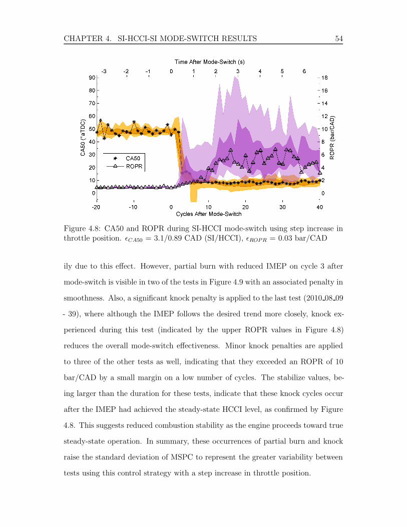
CHAPTER 4. SI-HCCI-SI MODE-SWITCH RESULTS 54
Figure 4.8: CA50 and ROPR during SI-HCCI mode-switch using step increase inthrottle position. εCA50 = 3.1/0.89 CAD (SI/HCCI), εROPR = 0.03 bar/CAD
ily due to this effect. However, partial burn with reduced IMEP on cycle 3 after
mode-switch is visible in two of the tests in Figure 4.9 with an associated penalty in
smoothness. Also, a significant knock penalty is applied to the last test (2010 08 09
- 39), where although the IMEP follows the desired trend more closely, knock ex-
perienced during this test (indicated by the upper ROPR values in Figure 4.8)
reduces the overall mode-switch effectiveness. Minor knock penalties are applied
to three of the other tests as well, indicating that they exceeded an ROPR of 10
bar/CAD by a small margin on a low number of cycles. The stabilize values, be-
ing larger than the duration for these tests, indicate that these knock cycles occur
after the IMEP had achieved the steady-state HCCI level, as confirmed by Figure
4.8. This suggests reduced combustion stability as the engine proceeds toward true
steady-state operation. In summary, these occurrences of partial burn and knock
raise the standard deviation of MSPC to represent the greater variability between
tests using this control strategy with a step increase in throttle position.
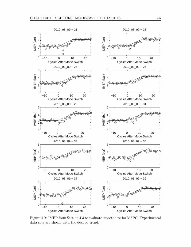
CHAPTER 4. SI-HCCI-SI MODE-SWITCH RESULTS 55
−10 0 10 200
2
4
6
Cycles After Mode Switch
IME
P (
bar)
2010_08_09 − 21
−10 0 10 200
2
4
6
Cycles After Mode Switch
IME
P (
bar)
2010_08_09 − 23
−10 0 10 200
2
4
6
Cycles After Mode Switch
IME
P (
bar)
2010_08_09 − 25
−10 0 10 200
2
4
6
Cycles After Mode SwitchIM
EP
(ba
r)
2010_08_09 − 27
−10 0 10 200
2
4
6
Cycles After Mode Switch
IME
P (
bar)
2010_08_09 − 29
−10 0 10 200
2
4
6
Cycles After Mode Switch
IME
P (
bar)
2010_08_09 − 31
−10 0 10 200
2
4
6
Cycles After Mode Switch
IME
P (
bar)
2010_08_09 − 33
−10 0 10 200
2
4
6
Cycles After Mode Switch
IME
P (
bar)
2010_08_09 − 35
−10 0 10 200
2
4
6
Cycles After Mode Switch
IME
P (
bar)
2010_08_09 − 37
−10 0 10 200
2
4
6
Cycles After Mode Switch
IME
P (
bar)
2010_08_09 − 39
Figure 4.9: IMEP from Section 4.3 to evaluate smoothness for MSPC. Experimentaldata sets are shown with the desired trend.
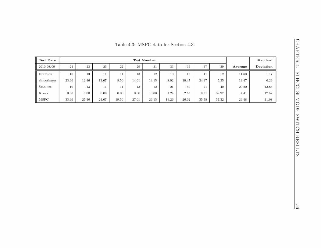
CHAPTER
4.SI-H
CCI-S
IMODE-SW
ITCH
RESULTS
56
Table 4.3: MSPC data for Section 4.3.
Test Date Test Number Standard
2010 08 09 21 23 25 27 29 31 33 35 37 39 Average Deviation
Duration 10 13 11 11 13 12 10 13 11 12 11.60 1.17
Smoothness 23.66 12.46 13.67 8.50 14.01 14.15 8.02 10.47 24.47 5.35 13.47 6.29
Stabilize 10 13 11 11 13 12 21 50 21 40 20.20 13.85
Knock 0.00 0.00 0.00 0.00 0.00 0.00 1.24 2.55 0.31 39.97 4.41 12.52
MSPC 33.66 25.46 24.67 19.50 27.01 26.15 19.26 26.02 35.78 57.32 29.48 11.08
CHAPTER 4. SI-HCCI-SI MODE-SWITCH RESULTS 57
4.4 SI-HCCI: CNG Injection Timing
One main goal of this thesis is to control SI-HCCI mode-switching using only
actuators available on standard engines. To mitigate the variability of combustion
for early HCCI mode cycles in Figures 4.6-4.8, a cycle by cycle fast actuator is
needed. CNG injection timing influences charge stratification during SI operation
[54] and is found to influence HCCI ignition as well. Early injection at IVC of the
previous cycle provides more stable operation in SI at the high intake temperatures
used for mode-switching, while advancing the injection toward IVO (moving the
injection timing to the right in Figure 3.14) has the effect of promoting auto-ignition
in HCCI.
Starting with the fuel sequence from the previous test in Figures 4.6-4.8, fuel
injection timing is added to assist ignition during the unstable cycles. Minor ad-
justments are then made to the fuel values to compensate for improved combustion.
Figure 4.10 shows the resulting mode-switch which has reduced uncertainty during
the early cycles compared to Figure 4.6. The cylinder pressures in Figure 4.11 show
that although not ideal, combustion is occurring on all cycles.
A smooth transition for CA50 between the two steady state values, along with
ROPR showing some cases of knock in the early cycles but rarely thereafter, is
shown in Figure 4.12. The drop in ROPR visible at the end of the sample test is
due to the PI fuel controller overcompensating and not a sign of ensuing misfire.
The SI-HCCI mode-switch transition time using this control strategy can not
be easily reduced without inducing knock. The slow increase in fuel delivery is
designed to counter-act the natural advancing tendency of the engine as determined
previously in Figure 4.4, thus limiting IMEP throughout the process.
Advancing injection timing through the mode-switch carries an associated effect
of improved stability in HCCI, demonstrated by lower variability in all parameters
toward the end of the provided data. With all other conditions the same as previous
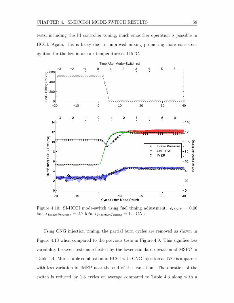
CHAPTER 4. SI-HCCI-SI MODE-SWITCH RESULTS 58
tests, including the PI controller tuning, much smoother operation is possible in
HCCI. Again, this is likely due to improved mixing promoting more consistent
ignition for the low intake air temperature of 115 ◦C.
−20 −10 0 10 20 30 400
200
400
600
CN
G T
imin
g (°
bIV
O)
−3 −2 −1 0 1 2 3 4 5 6
Time After Mode−Switch (s)
Figure 4.10: SI-HCCI mode-switch using fuel timing adjustment. εIMEP = 0.06bar, εIntakePressure = 2.7 kPa, εInjectionT iming = 1.1 CAD
Using CNG injection timing, the partial burn cycles are removed as shown in
Figure 4.13 when compared to the previous tests in Figure 4.9. This signifies less
variability between tests as reflected by the lower standard deviation of MSPC in
Table 4.4. More stable combustion in HCCI with CNG injection at IVO is apparent
with less variation in IMEP near the end of the transition. The duration of the
switch is reduced by 1.3 cycles on average compared to Table 4.3 along with a
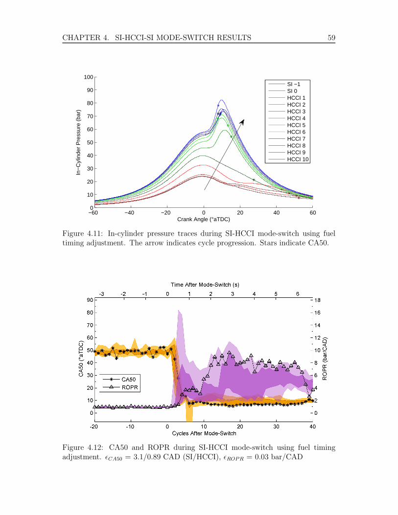
CHAPTER 4. SI-HCCI-SI MODE-SWITCH RESULTS 59
−60 −40 −20 0 20 40 600
10
20
30
40
50
60
70
80
90
100
Crank Angle (°aTDC)
In−
Cyl
inde
r P
ress
ure
(bar
)
SI −1SI 0HCCI 1HCCI 2HCCI 3HCCI 4HCCI 5HCCI 6HCCI 7HCCI 8HCCI 9HCCI 10
Figure 4.11: In-cylinder pressure traces during SI-HCCI mode-switch using fueltiming adjustment. The arrow indicates cycle progression. Stars indicate CA50.
Figure 4.12: CA50 and ROPR during SI-HCCI mode-switch using fuel timingadjustment. εCA50 = 3.1/0.89 CAD (SI/HCCI), εROPR = 0.03 bar/CAD

CHAPTER 4. SI-HCCI-SI MODE-SWITCH RESULTS 60
reduction in smoothness of 5.8 on average. Knock is only present in two of the
tests and much less significant than before. All these effects combine to reduce the
average MSPC by 10.5, or approximately one third, compared to Table 4.3 without
CNG timing adjustment.
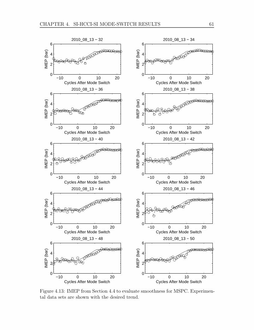
CHAPTER 4. SI-HCCI-SI MODE-SWITCH RESULTS 61
−10 0 10 200
2
4
6
Cycles After Mode Switch
IME
P (
bar)
2010_08_13 − 32
−10 0 10 200
2
4
6
Cycles After Mode Switch
IME
P (
bar)
2010_08_13 − 34
−10 0 10 200
2
4
6
Cycles After Mode Switch
IME
P (
bar)
2010_08_13 − 36
−10 0 10 200
2
4
6
Cycles After Mode SwitchIM
EP
(ba
r)
2010_08_13 − 38
−10 0 10 200
2
4
6
Cycles After Mode Switch
IME
P (
bar)
2010_08_13 − 40
−10 0 10 200
2
4
6
Cycles After Mode Switch
IME
P (
bar)
2010_08_13 − 42
−10 0 10 200
2
4
6
Cycles After Mode Switch
IME
P (
bar)
2010_08_13 − 44
−10 0 10 200
2
4
6
Cycles After Mode Switch
IME
P (
bar)
2010_08_13 − 46
−10 0 10 200
2
4
6
Cycles After Mode Switch
IME
P (
bar)
2010_08_13 − 48
−10 0 10 200
2
4
6
Cycles After Mode Switch
IME
P (
bar)
2010_08_13 − 50
Figure 4.13: IMEP from Section 4.4 to evaluate smoothness for MSPC. Experimen-tal data sets are shown with the desired trend.

CHAPTER
4.SI-H
CCI-S
IMODE-SW
ITCH
RESULTS
62
Table 4.4: MSPC data for Section 4.4.
Test Date Test Number Standard
2010 08 13 32 34 36 38 40 42 44 46 48 50 Average Deviation
Duration 8 9 11 9 10 12 11 11 11 11 10.30 1.25
Smoothness 8.21 6.20 10.20 5.73 5.69 7.13 5.77 7.65 10.40 10.05 7.70 1.93
Stabilize 8 18 11 20 10 12 11 11 11 11 12.30 3.71
Knock 0.00 0.01 0.00 3.45 0.00 0.00 0.00 0.00 0.00 5.99 0.94 2.08
MSPC 16.21 15.21 21.20 18.18 15.69 19.13 16.77 18.65 21.40 27.04 18.95 3.56
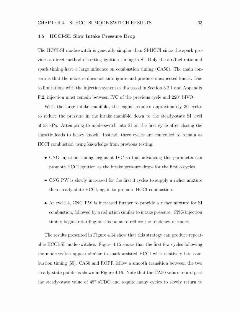
CHAPTER 4. SI-HCCI-SI MODE-SWITCH RESULTS 63
4.5 HCCI-SI: Slow Intake Pressure Drop
The HCCI-SI mode-switch is generally simpler than SI-HCCI since the spark pro-
vides a direct method of setting ignition timing in SI. Only the air/fuel ratio and
spark timing have a large influence on combustion timing (CA50). The main con-
cern is that the mixture does not auto ignite and produce unexpected knock. Due
to limitations with the injection system as discussed in Section 3.2.1 and Appendix
F.2, injection must remain between IVC of the previous cycle and 220◦ bIVO.
With the large intake manifold, the engine requires approximately 30 cycles
to reduce the pressure in the intake manifold down to the steady-state SI level
of 53 kPa. Attempting to mode-switch into SI on the first cycle after closing the
throttle leads to heavy knock. Instead, three cycles are controlled to remain as
HCCI combustion using knowledge from previous testing:� CNG injection timing begins at IVC so that advancing this parameter can
promote HCCI ignition as the intake pressure drops for the first 3 cycles.� CNG PW is slowly increased for the first 3 cycles to supply a richer mixture
then steady-state HCCI, again to promote HCCI combustion.� At cycle 4, CNG PW is increased further to provide a richer mixture for SI
combustion, followed by a reduction similar to intake pressure. CNG injection
timing begins retarding at this point to reduce the tendency of knock.
The results presented in Figure 4.14 show that this strategy can produce repeat-
able HCCI-SI mode-switches. Figure 4.15 shows that the first few cycles following
the mode-switch appear similar to spark-assisted HCCI with relatively late com-
bustion timing [55]. CA50 and ROPR follow a smooth transition between the two
steady-state points as shown in Figure 4.16. Note that the CA50 values retard past
the steady-state value of 48◦ aTDC and require many cycles to slowly return to
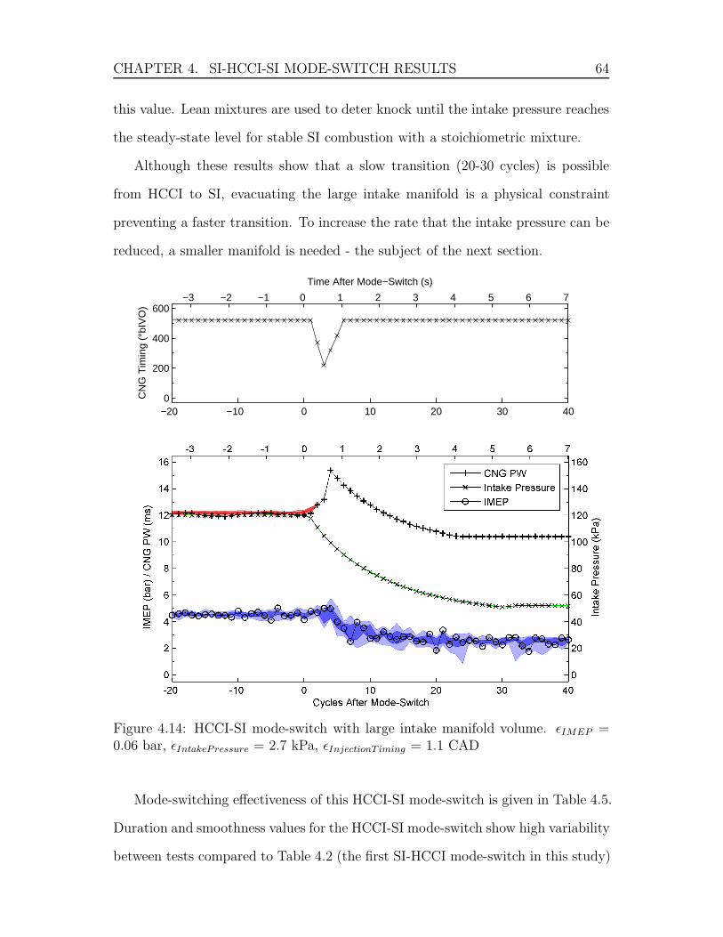
CHAPTER 4. SI-HCCI-SI MODE-SWITCH RESULTS 64
this value. Lean mixtures are used to deter knock until the intake pressure reaches
the steady-state level for stable SI combustion with a stoichiometric mixture.
Although these results show that a slow transition (20-30 cycles) is possible
from HCCI to SI, evacuating the large intake manifold is a physical constraint
preventing a faster transition. To increase the rate that the intake pressure can be
reduced, a smaller manifold is needed - the subject of the next section.
−20 −10 0 10 20 30 400
200
400
600
CN
G T
imin
g (°
bIV
O)
−3 −2 −1 0 1 2 3 4 5 6 7
Time After Mode−Switch (s)
Figure 4.14: HCCI-SI mode-switch with large intake manifold volume. εIMEP =0.06 bar, εIntakePressure = 2.7 kPa, εInjectionT iming = 1.1 CAD
Mode-switching effectiveness of this HCCI-SI mode-switch is given in Table 4.5.
Duration and smoothness values for the HCCI-SI mode-switch show high variability
between tests compared to Table 4.2 (the first SI-HCCI mode-switch in this study)
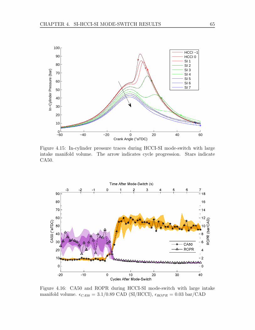
CHAPTER 4. SI-HCCI-SI MODE-SWITCH RESULTS 65
−60 −40 −20 0 20 40 600
10
20
30
40
50
60
70
80
90
100
Crank Angle (°aTDC)
In−
Cyl
inde
r P
ress
ure
(bar
)
HCCI −1HCCI 0SI 1SI 2SI 3SI 4SI 5SI 6SI 7
Figure 4.15: In-cylinder pressure traces during HCCI-SI mode-switch with largeintake manifold volume. The arrow indicates cycle progression. Stars indicateCA50.
Figure 4.16: CA50 and ROPR during HCCI-SI mode-switch with large intakemanifold volume. εCA50 = 3.1/0.89 CAD (SI/HCCI), εROPR = 0.03 bar/CAD

CHAPTER 4. SI-HCCI-SI MODE-SWITCH RESULTS 66
associated with fluctuations in IMEP visible in Figure 4.5. COV IMEP in SI at this
operating point is 11% requiring MSPC to be adjusted to determine the end of the
mode-switch as discussed in Chapter 3. This low stability in the final combustion
mode increases difficulty achieving a smooth and quick mode-switch, leading to the
high average and standard deviation in MSPC for this control strategy.
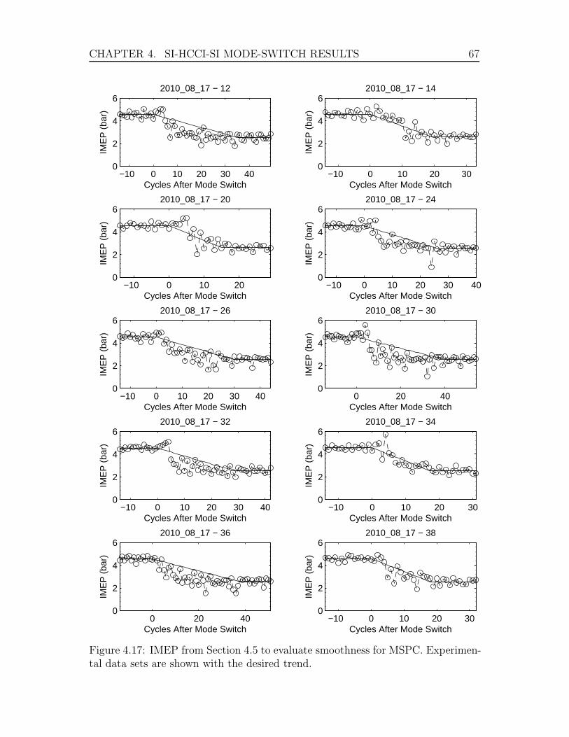
CHAPTER 4. SI-HCCI-SI MODE-SWITCH RESULTS 67
−10 0 10 20 30 400
2
4
6
Cycles After Mode Switch
IME
P (
bar)
2010_08_17 − 12
−10 0 10 20 300
2
4
6
Cycles After Mode Switch
IME
P (
bar)
2010_08_17 − 14
−10 0 10 200
2
4
6
Cycles After Mode Switch
IME
P (
bar)
2010_08_17 − 20
−10 0 10 20 30 400
2
4
6
Cycles After Mode SwitchIM
EP
(ba
r)
2010_08_17 − 24
−10 0 10 20 30 400
2
4
6
Cycles After Mode Switch
IME
P (
bar)
2010_08_17 − 26
0 20 400
2
4
6
Cycles After Mode Switch
IME
P (
bar)
2010_08_17 − 30
−10 0 10 20 30 400
2
4
6
Cycles After Mode Switch
IME
P (
bar)
2010_08_17 − 32
−10 0 10 20 300
2
4
6
Cycles After Mode Switch
IME
P (
bar)
2010_08_17 − 34
0 20 400
2
4
6
Cycles After Mode Switch
IME
P (
bar)
2010_08_17 − 36
−10 0 10 20 300
2
4
6
Cycles After Mode Switch
IME
P (
bar)
2010_08_17 − 38
Figure 4.17: IMEP from Section 4.5 to evaluate smoothness for MSPC. Experimen-tal data sets are shown with the desired trend.

CHAPTER
4.SI-H
CCI-S
IMODE-SW
ITCH
RESULTS
68
Table 4.5: MSPC data for Section 4.5.
Test Date Test Number Standard
2010 08 17 12 14 20 24 26 30 32 34 36 38 Average Deviation
Duration 35 19 15 26 30 40 28 17 37 18 26.50 9.01
Smoothness 55.78 18.25 21.64 38.44 47.12 81.94 42.30 17.50 66.78 19.74 40.95 22.36
Stabilize 35 19 15 26 30 40 28 17 37 18 26.50 9.01
Knock 0.00 0.00 0.00 0.00 0.00 0.00 0.00 0.00 0.00 0.00 0.00 0.00
MSPC 90.78 37.25 36.64 64.44 77.12 121.94 70.30 34.50 103.78 37.74 67.45 31.22
CHAPTER 4. SI-HCCI-SI MODE-SWITCH RESULTS 69
4.6 Steady-State Operating Conditions - Small Manifold
The intake manifold is modified to 0.5 L so the volume downstream of the electronic
throttle is approximately one engine displacement. This is typical for production
engines and allows for quicker changes in intake pressure. Based on the change
in intake response, a slightly modified set of compatible steady-state operating
conditions to mode-switch between are summarized in Table 4.6.
Air mass flow rate is maintained at the same level for both SI and HCCI as with
the large manifold in Table 4.6. The measurement of P IVC at these flow rates is
recorded and used as the set point. Intake air temperature is increased to achieve
the same mixture temperature in HCCI, leading to a cooler mixture in SI due to
several factors explored in Appendix C. The lower mixture temperatures in SI leads
to more stable combustion and reduced tendency toward knock, but otherwise SI
operation is similar to previous testing.
CNG injection timing is advanced to IVO during the SI-HCCI mode-switch;
however, timing must be retarded to allow for HCCI-SI mode-switching without
a misfire resulting from the controller limitation described in Section 3.2.1 and
Appendix F.2. CNG PW is not set directly in HCCI, but as before is controlled
toward a ROPR value of 6 bar/CAD for stable HCCI operation. With the other
conditions adjusted as described above, the resulting leaner mixtures lead to a
lower IMEP in HCCI. With the focus of this mode-switching development being to
achieve stable HCCI combustion, the reduction in IMEP, compared with previous
testing using the large intake manifold, is accepted as the most stable HCCI op-
erating point using the small intake manifold. Variation of IMEP in both SI and
HCCI steady-state combustion modes surrounding a mode-switch is the topic of
Section 4.11.

CHAPTER 4. SI-HCCI-SI MODE-SWITCH RESULTS 70
Table 4.6: Steady-state operating conditions for mode-switching tests - small(0.5 L) intake manifold.
Set Points SI HCCICNG System Pressure 5.5 bar 5.5 barEffective Compression Ratio 17.0 17.0Engine Speed 700 RPM 700 RPMIntake Air Temperature 140 ◦C 140 ◦CP IVC 58 kPa 113 kPaSpark Timing 5◦ aTDC -ActuatorsCNG Injection Timing 520◦ bIVO 200◦ bIVOCNG Pulse Width 10.6 ms ∼10.4 msThrottle Position 28% 86%MeasurementsAir Mass Flow 1.3 g/s 3.4 g/sCNG Mass Flow 74 mg/s 72 mg/sEquivalence Ratio 1.0 0.37Exhaust Pressure 91 kPa 92 kPaExhaust Temperature 460 ◦C 250 ◦CMixture Temperature 85 ◦C 102 ◦CCalculatedCA50 49◦ aTDC 5◦ aTDCCOV IMEP 3% 3%IMEP 2.8 bar 3.5 barROPR 0.8 bar/CAD 6.0 bar/CADThermal Efficiency 27% 35%Exhaust EmissionsCarbon Monoxide (CO) 0.08% 0.10%Carbon Dioxide (CO2) 10% 3.7%Hydrocarbons (HC) 1600 ppm 3500 ppmOxides of Nitrogen (NOx) 690 ppm 9 ppmOxygen (O2) 1.8% 14%
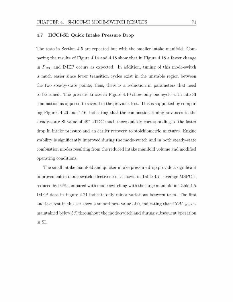
CHAPTER 4. SI-HCCI-SI MODE-SWITCH RESULTS 71
4.7 HCCI-SI: Quick Intake Pressure Drop
The tests in Section 4.5 are repeated but with the smaller intake manifold. Com-
paring the results of Figure 4.14 and 4.18 show that in Figure 4.18 a faster change
in P IVC and IMEP occurs as expected. In addition, tuning of this mode-switch
is much easier since fewer transition cycles exist in the unstable region between
the two steady-state points; thus, there is a reduction in parameters that need
to be tuned. The pressure traces in Figure 4.19 show only one cycle with late SI
combustion as opposed to several in the previous test. This is supported by compar-
ing Figures 4.20 and 4.16, indicating that the combustion timing advances to the
steady-state SI value of 49◦ aTDC much more quickly corresponding to the faster
drop in intake pressure and an earlier recovery to stoichiometric mixtures. Engine
stability is significantly improved during the mode-switch and in both steady-state
combustion modes resulting from the reduced intake manifold volume and modified
operating conditions.
The small intake manifold and quicker intake pressure drop provide a significant
improvement in mode-switch effectiveness as shown in Table 4.7 - average MSPC is
reduced by 94% compared with mode-switching with the large manifold in Table 4.5.
IMEP data in Figure 4.21 indicate only minor variations between tests. The first
and last test in this set show a smoothness value of 0, indicating that COV IMEP is
maintained below 5% throughout the mode-switch and during subsequent operation
in SI.

CHAPTER 4. SI-HCCI-SI MODE-SWITCH RESULTS 72
−20 −10 0 10 20 30 400
200
400
600
CN
G T
imin
g (°
bIV
O)
−3 −2 −1 0 1 2 3 4 5 6
Time After Mode−Switch (s)
Figure 4.18: HCCI-SI mode-switch with reduced intake manifold volume. εIMEP
= 0.06 bar, εPIV C = 2.8 kPa, εInjectionT iming = 1.1 CAD
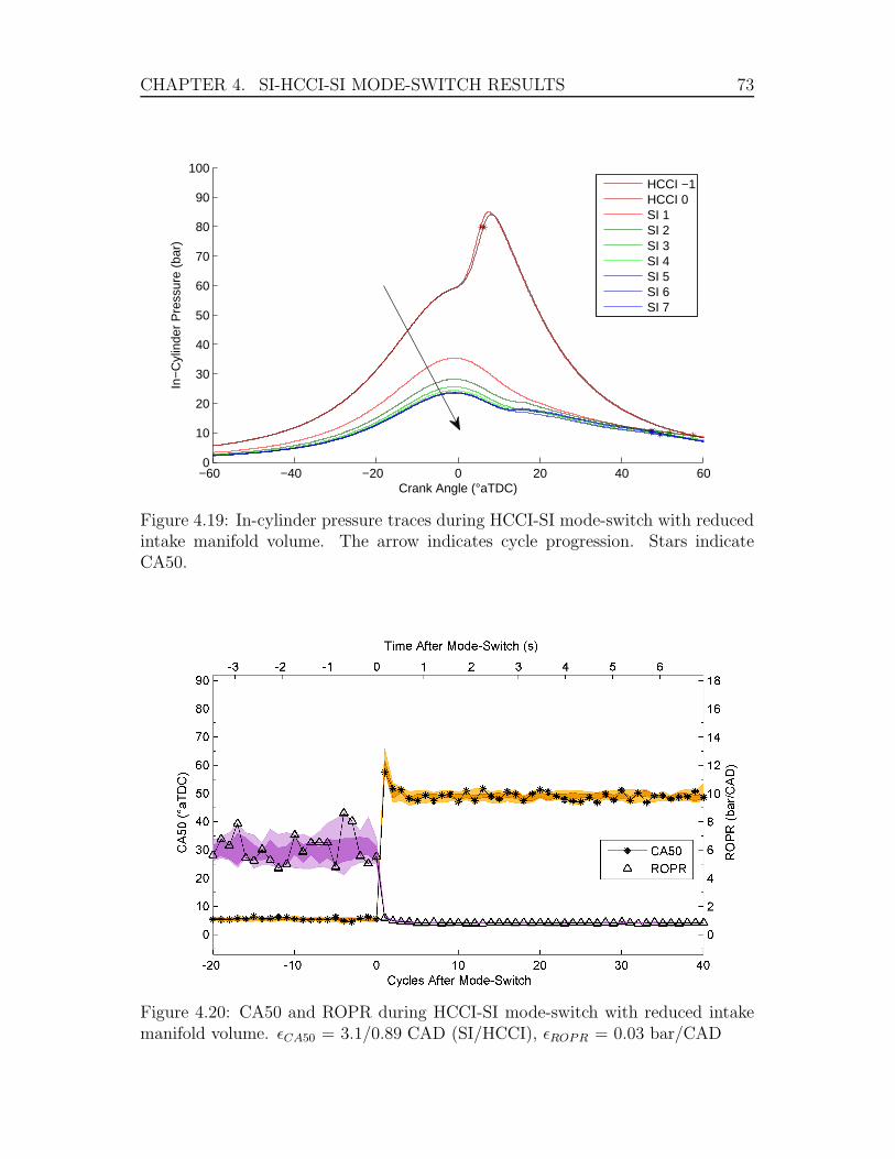
CHAPTER 4. SI-HCCI-SI MODE-SWITCH RESULTS 73
−60 −40 −20 0 20 40 600
10
20
30
40
50
60
70
80
90
100
Crank Angle (°aTDC)
In−
Cyl
inde
r P
ress
ure
(bar
)
HCCI −1HCCI 0SI 1SI 2SI 3SI 4SI 5SI 6SI 7
Figure 4.19: In-cylinder pressure traces during HCCI-SI mode-switch with reducedintake manifold volume. The arrow indicates cycle progression. Stars indicateCA50.
Figure 4.20: CA50 and ROPR during HCCI-SI mode-switch with reduced intakemanifold volume. εCA50 = 3.1/0.89 CAD (SI/HCCI), εROPR = 0.03 bar/CAD
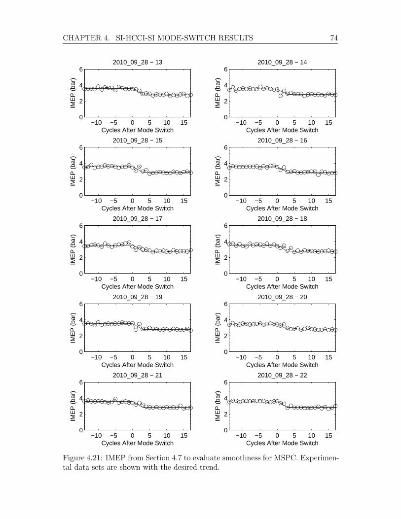
CHAPTER 4. SI-HCCI-SI MODE-SWITCH RESULTS 74
−10 −5 0 5 10 150
2
4
6
Cycles After Mode Switch
IME
P (
bar)
2010_09_28 − 13
−10 −5 0 5 10 150
2
4
6
Cycles After Mode Switch
IME
P (
bar)
2010_09_28 − 14
−10 −5 0 5 10 150
2
4
6
Cycles After Mode Switch
IME
P (
bar)
2010_09_28 − 15
−10 −5 0 5 10 150
2
4
6
Cycles After Mode SwitchIM
EP
(ba
r)
2010_09_28 − 16
−10 −5 0 5 10 150
2
4
6
Cycles After Mode Switch
IME
P (
bar)
2010_09_28 − 17
−10 −5 0 5 10 150
2
4
6
Cycles After Mode Switch
IME
P (
bar)
2010_09_28 − 18
−10 −5 0 5 10 150
2
4
6
Cycles After Mode Switch
IME
P (
bar)
2010_09_28 − 19
−10 −5 0 5 10 150
2
4
6
Cycles After Mode Switch
IME
P (
bar)
2010_09_28 − 20
−10 −5 0 5 10 150
2
4
6
Cycles After Mode Switch
IME
P (
bar)
2010_09_28 − 21
−10 −5 0 5 10 150
2
4
6
Cycles After Mode Switch
IME
P (
bar)
2010_09_28 − 22
Figure 4.21: IMEP from Section 4.7 to evaluate smoothness for MSPC. Experimen-tal data sets are shown with the desired trend.

CHAPTER
4.SI-H
CCI-S
IMODE-SW
ITCH
RESULTS
75
Table 4.7: MSPC data for Section 4.7.
Test Date Test Number Standard
2010 09 28 13 14 15 16 17 18 19 20 21 22 Average Deviation
Duration 3 3 3 3 3 3 3 3 3 3 3.00 0.00
Smoothness 0.00 1.69 1.19 0.43 0.70 0.55 1.86 0.57 0.66 0.00 0.77 0.63
Stabilize 3 3 3 3 3 3 3 3 3 3 3.00 0.00
Knock 0.00 0.00 0.00 0.00 0.00 0.00 0.00 0.00 0.00 0.00 0.00 0.00
MSPC 3.00 4.69 4.19 3.43 3.70 3.55 4.86 3.57 3.66 3.00 3.77 0.63
CHAPTER 4. SI-HCCI-SI MODE-SWITCH RESULTS 76
4.8 SI-HCCI: Optimized Scenario
The small manifold allows for finer control over air induction on individual cycles.
Charge mass has the largest influence on ignition timing for HCCI with conventional
actuation, especially during the early cycles following an SI-HCCI mode-switch.
To improve SI-HCCI mode-switching, air delivery is tailored to meet combustion
requirements for individual cycles.
The benefits of this approach can be seen in the test results given in Figure 4.22.
A one-cycle step in IMEP to the new steady-state value reduces the duration of the
switch to 1 cycle, the ideal case. Controls are adjusted over the subsequent cycles
to maintain a nearly constant IMEP output as the engine itself stabilizes to the new
operating condition. Figure 4.23 shows the first transition cycle (HCCI 1) occurring
with a pressure trend indicative of a hybrid between SI and HCCI combustion. The
pressure rise begins at nearly the same location as the steady-state SI cycles (SI
-1 and SI 0), but with a more significant pressure rise similar to HCCI combustion
(all subsequent cycles). This is a result of the some early SI flame propagation
leading to HCCI ignition with the hot SI combustion and residual gases in the
combustion chamber. The next cycle (HCCI 2) is not quite at steady-state intake
pressure, as indicated by the lower overall cylinder pressure, but shows good HCCI
combustion with appropriate combustion timing (CA50). Subsequent cycles have
a slowly dropping and retarding peak pressure, but otherwise appear very stable.
Figure 4.24 supports these observations with a quick transition from the late SI
combustion timing to the earlier HCCI values. ROPR values represent the visible
change in combustion severity in the cylinder pressure traces, followed by a smooth
transition toward the controlled value of 6 bar/CAD. Again, the two CA50 values
shown for cycles 2 and 3 after mode-switch are retarded compared to future cycles
due to their evaluation using SI coefficients in the Woschni equations since the
spark is still activated.
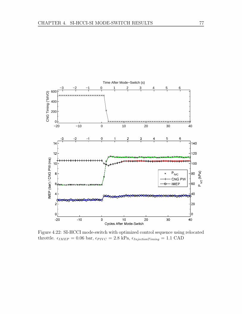
CHAPTER 4. SI-HCCI-SI MODE-SWITCH RESULTS 77
−20 −10 0 10 20 30 400
200
400
600
CN
G T
imin
g (°
bIV
O)
−3 −2 −1 0 1 2 3 4 5 6
Time After Mode−Switch (s)
Figure 4.22: SI-HCCI mode-switch with optimized control sequence using relocatedthrottle. εIMEP = 0.06 bar, εPIV C = 2.8 kPa, εInjectionT iming = 1.1 CAD
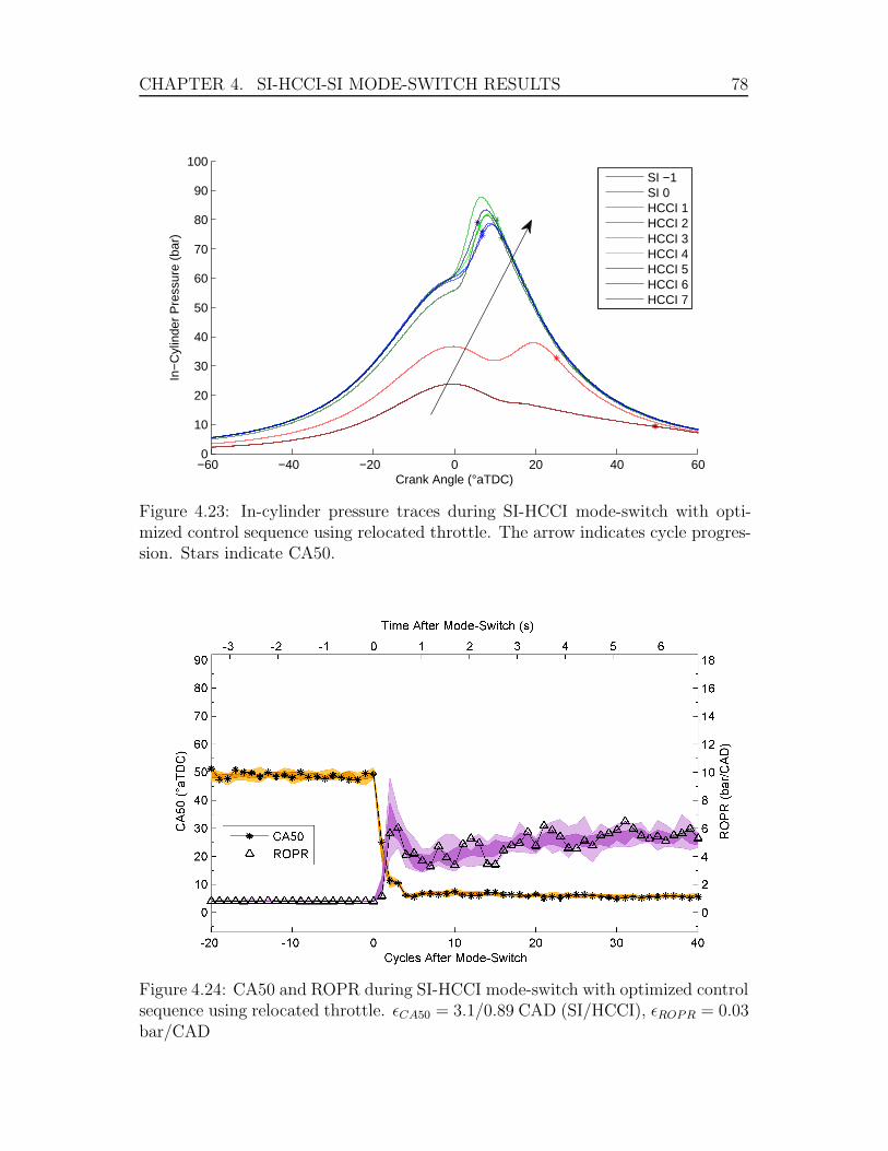
CHAPTER 4. SI-HCCI-SI MODE-SWITCH RESULTS 78
−60 −40 −20 0 20 40 600
10
20
30
40
50
60
70
80
90
100
Crank Angle (°aTDC)
In−
Cyl
inde
r P
ress
ure
(bar
)
SI −1SI 0HCCI 1HCCI 2HCCI 3HCCI 4HCCI 5HCCI 6HCCI 7
Figure 4.23: In-cylinder pressure traces during SI-HCCI mode-switch with opti-mized control sequence using relocated throttle. The arrow indicates cycle progres-sion. Stars indicate CA50.
Figure 4.24: CA50 and ROPR during SI-HCCI mode-switch with optimized controlsequence using relocated throttle. εCA50 = 3.1/0.89 CAD (SI/HCCI), εROPR = 0.03bar/CAD

CHAPTER 4. SI-HCCI-SI MODE-SWITCH RESULTS 79
MSPC data for these tests is given in Table 4.8, showing that mode-switch
effectiveness based on the developed criteria is ideal. IMEP data in Figure 4.25
supports this with a step change and subsequent smooth operation visible in all
tests.
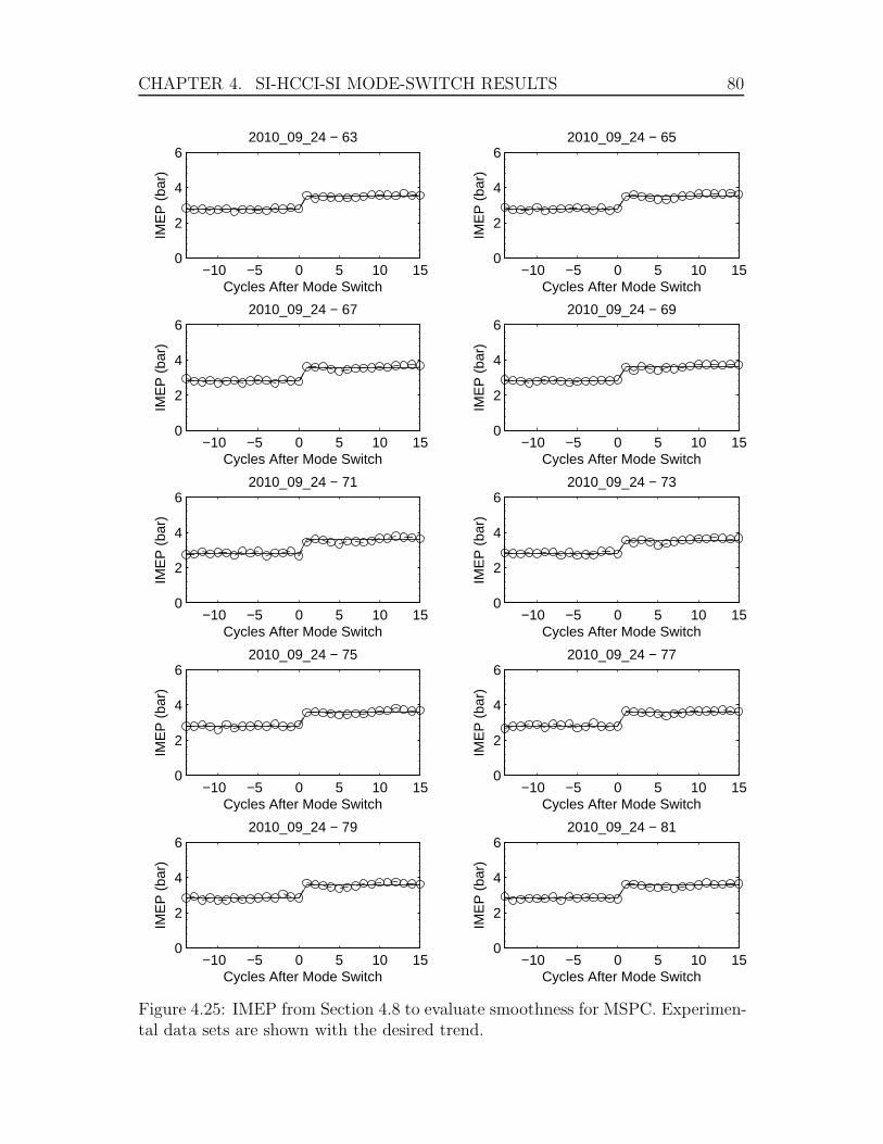
CHAPTER 4. SI-HCCI-SI MODE-SWITCH RESULTS 80
−10 −5 0 5 10 150
2
4
6
Cycles After Mode Switch
IME
P (
bar)
2010_09_24 − 63
−10 −5 0 5 10 150
2
4
6
Cycles After Mode Switch
IME
P (
bar)
2010_09_24 − 65
−10 −5 0 5 10 150
2
4
6
Cycles After Mode Switch
IME
P (
bar)
2010_09_24 − 67
−10 −5 0 5 10 150
2
4
6
Cycles After Mode SwitchIM
EP
(ba
r)
2010_09_24 − 69
−10 −5 0 5 10 150
2
4
6
Cycles After Mode Switch
IME
P (
bar)
2010_09_24 − 71
−10 −5 0 5 10 150
2
4
6
Cycles After Mode Switch
IME
P (
bar)
2010_09_24 − 73
−10 −5 0 5 10 150
2
4
6
Cycles After Mode Switch
IME
P (
bar)
2010_09_24 − 75
−10 −5 0 5 10 150
2
4
6
Cycles After Mode Switch
IME
P (
bar)
2010_09_24 − 77
−10 −5 0 5 10 150
2
4
6
Cycles After Mode Switch
IME
P (
bar)
2010_09_24 − 79
−10 −5 0 5 10 150
2
4
6
Cycles After Mode Switch
IME
P (
bar)
2010_09_24 − 81
Figure 4.25: IMEP from Section 4.8 to evaluate smoothness for MSPC. Experimen-tal data sets are shown with the desired trend.

CHAPTER
4.SI-H
CCI-S
IMODE-SW
ITCH
RESULTS
81
Table 4.8: MSPC data for Section 4.8.
Test Date Test Number Standard
2010 09 24 63 65 67 69 71 73 75 77 79 81 Average Deviation
Duration 1 1 1 1 1 1 1 1 1 1 1.00 0.00
Smoothness 0.00 0.00 0.00 0.00 0.00 0.00 0.00 0.00 0.00 0.00 0.00 0.00
Stabilize 1 1 1 1 1 1 1 1 1 1 1.00 0.00
Knock 0.00 0.00 0.00 0.00 0.00 0.00 0.00 0.00 0.00 0.00 0.00 0.00
MSPC 1.00 1.00 1.00 1.00 1.00 1.00 1.00 1.00 1.00 1.00 1.00 0.00
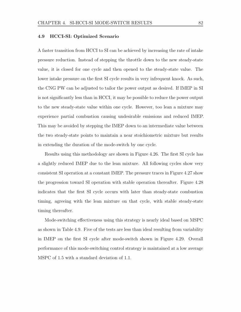
CHAPTER 4. SI-HCCI-SI MODE-SWITCH RESULTS 82
4.9 HCCI-SI: Optimized Scenario
A faster transition from HCCI to SI can be achieved by increasing the rate of intake
pressure reduction. Instead of stepping the throttle down to the new steady-state
value, it is closed for one cycle and then opened to the steady-state value. The
lower intake pressure on the first SI cycle results in very infrequent knock. As such,
the CNG PW can be adjusted to tailor the power output as desired. If IMEP in SI
is not significantly less than in HCCI, it may be possible to reduce the power output
to the new steady-state value within one cycle. However, too lean a mixture may
experience partial combustion causing undesirable emissions and reduced IMEP.
This may be avoided by stepping the IMEP down to an intermediate value between
the two steady-state points to maintain a near stoichiometric mixture but results
in extending the duration of the mode-switch by one cycle.
Results using this methodology are shown in Figure 4.26. The first SI cycle has
a slightly reduced IMEP due to the lean mixture. All following cycles show very
consistent SI operation at a constant IMEP. The pressure traces in Figure 4.27 show
the progression toward SI operation with stable operation thereafter. Figure 4.28
indicates that the first SI cycle occurs with later than steady-state combustion
timing, agreeing with the lean mixture on that cycle, with stable steady-state
timing thereafter.
Mode-switching effectiveness using this strategy is nearly ideal based on MSPC
as shown in Table 4.9. Five of the tests are less than ideal resulting from variability
in IMEP on the first SI cycle after mode-switch shown in Figure 4.29. Overall
performance of this mode-switching control strategy is maintained at a low average
MSPC of 1.5 with a standard deviation of 1.1.
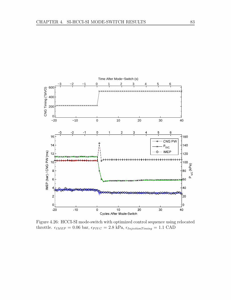
CHAPTER 4. SI-HCCI-SI MODE-SWITCH RESULTS 83
−20 −10 0 10 20 30 400
200
400
600
CN
G T
imin
g (°
bIV
O)
−3 −2 −1 0 1 2 3 4 5 6
Time After Mode−Switch (s)
Figure 4.26: HCCI-SI mode-switch with optimized control sequence using relocatedthrottle. εIMEP = 0.06 bar, εPIV C = 2.8 kPa, εInjectionT iming = 1.1 CAD
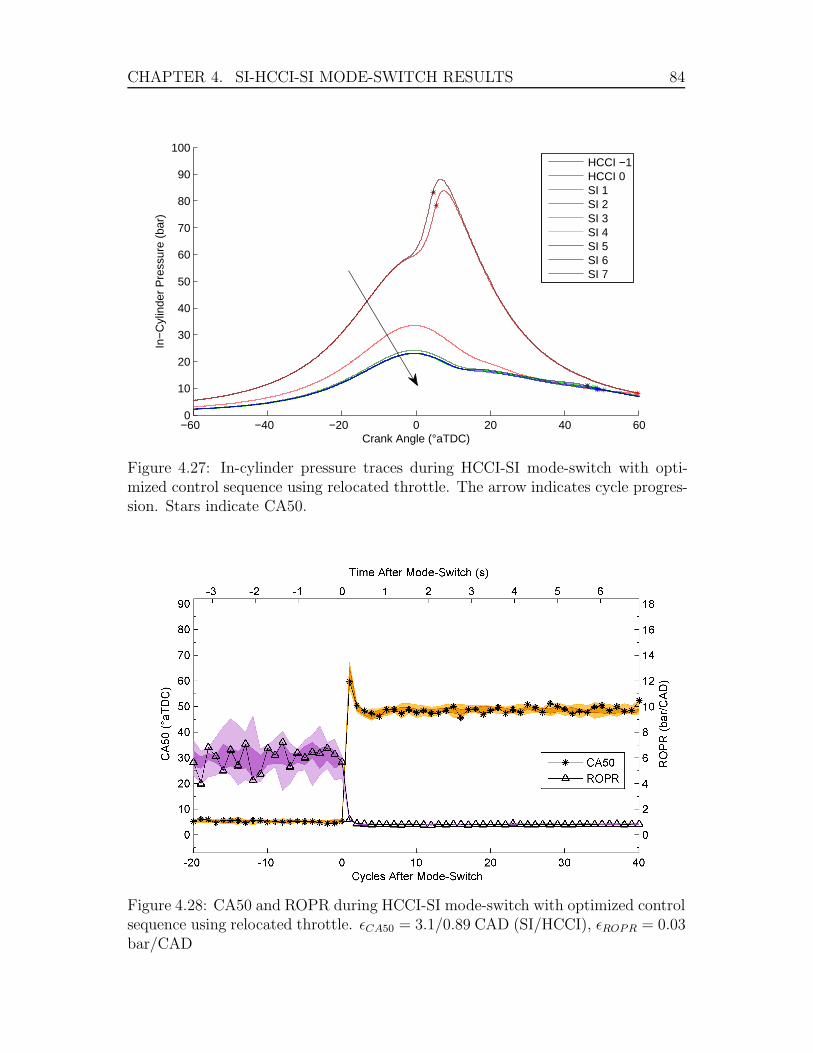
CHAPTER 4. SI-HCCI-SI MODE-SWITCH RESULTS 84
−60 −40 −20 0 20 40 600
10
20
30
40
50
60
70
80
90
100
Crank Angle (°aTDC)
In−
Cyl
inde
r P
ress
ure
(bar
)
HCCI −1HCCI 0SI 1SI 2SI 3SI 4SI 5SI 6SI 7
Figure 4.27: In-cylinder pressure traces during HCCI-SI mode-switch with opti-mized control sequence using relocated throttle. The arrow indicates cycle progres-sion. Stars indicate CA50.
Figure 4.28: CA50 and ROPR during HCCI-SI mode-switch with optimized controlsequence using relocated throttle. εCA50 = 3.1/0.89 CAD (SI/HCCI), εROPR = 0.03bar/CAD

CHAPTER 4. SI-HCCI-SI MODE-SWITCH RESULTS 85
−10 −5 0 5 10 150
2
4
6
Cycles After Mode Switch
IME
P (
bar)
2010_09_24 − 64
−10 −5 0 5 10 150
2
4
6
Cycles After Mode Switch
IME
P (
bar)
2010_09_24 − 68
−10 −5 0 5 10 150
2
4
6
Cycles After Mode Switch
IME
P (
bar)
2010_09_24 − 70
−10 −5 0 5 10 150
2
4
6
Cycles After Mode SwitchIM
EP
(ba
r)
2010_09_24 − 72
−10 −5 0 5 10 150
2
4
6
Cycles After Mode Switch
IME
P (
bar)
2010_09_24 − 74
−10 −5 0 5 10 150
2
4
6
Cycles After Mode Switch
IME
P (
bar)
2010_09_24 − 76
−10 −5 0 5 10 150
2
4
6
Cycles After Mode Switch
IME
P (
bar)
2010_09_24 − 78
−10 −5 0 5 10 150
2
4
6
Cycles After Mode Switch
IME
P (
bar)
2010_09_24 − 80
−10 −5 0 5 10 150
2
4
6
Cycles After Mode Switch
IME
P (
bar)
2010_09_24 − 82
−10 −5 0 5 10 150
2
4
6
Cycles After Mode Switch
IME
P (
bar)
2010_09_24 − 84
Figure 4.29: IMEP from Section 4.9 to evaluate smoothness for MSPC. Experimen-tal data sets are shown with the desired trend.

CHAPTER
4.SI-H
CCI-S
IMODE-SW
ITCH
RESULTS
86
Table 4.9: MSPC data for Section 4.9.
Test Date Test Number Standard
2010 09 24 64 68 70 72 74 76 78 80 82 84 Average Deviation
Duration 1 2 1 1 1 1 1 1 1 2 1.20 0.42
Smoothness 0.00 0.00 0.21 0.00 0.00 0.11 0.00 0.20 0.00 2.50 0.30 0.78
Stabilize 1 2 1 1 1 1 1 1 1 2 1.20 0.42
Knock 0.00 0.00 0.00 0.00 0.00 0.00 0.00 0.00 0.00 0.00 0.00 0.00
MSPC 1.00 2.00 1.21 1.00 1.00 1.11 1.00 1.20 1.00 4.50 1.50 1.10
CHAPTER 4. SI-HCCI-SI MODE-SWITCH RESULTS 87
4.10 Mode-Switching Sensitivity - Repeated SI-HCCI-SI Transitions
For real-world applications, it is possible that a need to mode-switch will occur
frequently. Depending on the sensitivity of the method used to induce the mode-
switch, this may not be possible without elaborate control schemes to adapt to un-
stable engine conditions. To investigate this aspect, a set of repeat mode-switches
are completed using the same optimized open-loop control sequences as in Sections
4.8 and 4.9. No adjustments have been made for the different operating conditions
experienced during these quick transitions as opposed to beginning in steady-state.
Disturbances exist in engine speed, mixture temperature, and the pressure in the
intake buffer tank, with the first two being measured values and presented in Fig-
ure 4.32. The limitation in CNG injection timing can not be avoided in this test
and one cycle in HCCI must intentionally misfire with no fuel delivered before
mode-switching back to SI. This further destabilizes the engine.
Test data are shown in Figures 4.30 and 4.31. Results are encouraging as the
mode-switching still completes in both directions with only a few partial burn cycles
during the HCCI-SI mode-switches. These are due to a lean mixture implemented
in Section 4.9 to smooth IMEP during the transition. Delivering more CNG on
the first SI cycle after these HCCI-SI mode-switches would remedy the partial
burn cycles experienced in this situation. Again, the first few cycles under HCCI
combustion are evaluated using Woschni heat transfer coefficients for SI while the
spark is still activated as discussed in Section 3.3.1.

CHAPTER 4. SI-HCCI-SI MODE-SWITCH RESULTS 88
0 50 100 150 200 250 30040
60
80
100
120
140
PIV
C (
kPa)
−5 0 5 10 15 20 25 30 35 40 45 50 55
Time After Mode−Switch (s)
0 50 100 150 200 250 300
10
12
14
CN
G P
W (
ms)
−5 0 5 10 15 20 25 30 35 40 45 50 55
0 50 100 150 200 250 3000
200
400
600
CN
G T
imin
g (°
bIV
O)
−5 0 5 10 15 20 25 30 35 40 45 50 55
0 50 100 150 200 250 300
1
2
3
4
Cycles After Mode−Switch
IME
P (
bar)
−5 0 5 10 15 20 25 30 35 40 45 50 55
Figure 4.30: Controls and IMEP during repeated SI-HCCI-SI mode-switching. LowP IVC and IMEP values correspond to SI and high values are HCCI. CNG PW andIMEP values falling below the lower edge indicate a misfire resulting from the nec-essary CNG timing adjustment. εIMEP = 0.06 bar, εPIV C = 2.8 kPa, εInjectionT iming
= 1.1 CAD

CHAPTER 4. SI-HCCI-SI MODE-SWITCH RESULTS 89
0 50 100 150 200 250 3000
20
40
60C
A50
(°a
TD
C)
−5 0 5 10 15 20 25 30 35 40 45 50 55
Time After Mode−Switch (s)
0 50 100 150 200 250 3000
2
4
6
8
10
Cycles After Mode−Switch
RO
PR
(ba
r/C
AD
)
−5 0 5 10 15 20 25 30 35 40 45 50 55
Figure 4.31: Combustion evaluation during repeated SI-HCCI-SI mode-switching.CA50 values falling below lower edge indicate a misfire resulting from CNG timingadjustment. SI and HCCI operation correspond with Figure 4.30. εCA50 = 3.1/0.89CAD (SI/HCCI), εROPR = 0.03 bar/CAD, εEquivalenceRatio = 12%
0 50 100 150 200 250 30080
85
90
95
100
Mix
ture
Tem
pera
ture
(°C
) −5 0 5 10 15 20 25 30 35 40 45 50 55
Time After Mode−Switch (s)
0 50 100 150 200 250 300680
690
700
710
720
Cycles After Mode−Switch
Eng
ine
Spe
ed (
RP
M)
−5 0 5 10 15 20 25 30 35 40 45 50 55
Figure 4.32: Disturbances experienced during repeated SI-HCCI-SI mode-switchingthat are not considered in the open-loop control sequence. SI and HCCI operationcorrespond with Figure 4.30.

CHAPTER 4. SI-HCCI-SI MODE-SWITCH RESULTS 90
4.11 Extension to Other Operating Points
In this section, a different operating speed is tested to show mode-switching po-
tential along with variability in IMEP for both SI and HCCI. The focus of this
research is directed toward large stationary engines, so a slower engine speed of
500 RPM is chosen. Slower engine speed induces some changes in HCCI combus-
tion, most notable being less memory effect between cycles, and less audible knock
at the same ROPR value.
Testing begins with an operating point similar to those presented in previous
mode-switching tests, although with cooler intake air temperature and slightly
advanced spark timing to increase IMEP in SI. Table 4.10 presents the variations
on this operating point to achieve higher and lower IMEP levels in both SI and
HCCI. Open-loop control sequences for fuel delivery and throttle positions are
developed in the same manner as described in sections 4.8 and 4.9. Figures 4.33,
and 4.37 present results for various IMEP levels in SI for both directions of mode-
switch, while Figure 4.35 and 4.39 present tests for different levels of IMEP during
HCCI operation. Calculated parameters including CA50, ROPR, and equivalence
ratio are provided in Figures 4.34, 4.38, 4.36, and 4.40 for the aforementioned test
data. Several observations are drawn from this information and are outlined in
Sections 5.4 and 5.4.
Mode-switch effectiveness for these tests with varying IMEP is presented in
Table 4.11. Most cases are optimized to an ideal case where MSPC is equal to 1;
however, four of the tests have some penalty. The only significant penalty occurs
for test 3 SI-HCCI due to knock that propagates after the mode-switch as shown
in Figure 4.36.
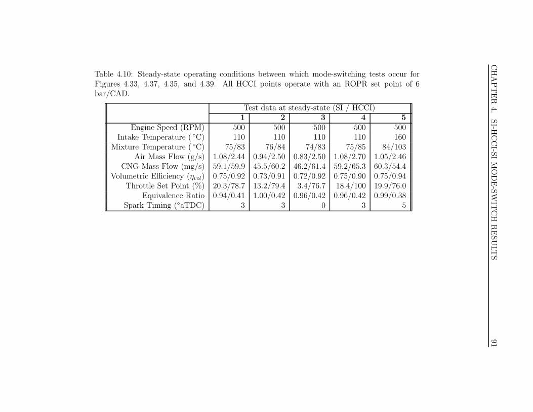
CHAPTER
4.SI-H
CCI-S
IMODE-SW
ITCH
RESULTS
91
Table 4.10: Steady-state operating conditions between which mode-switching tests occur forFigures 4.33, 4.37, 4.35, and 4.39. All HCCI points operate with an ROPR set point of 6bar/CAD.
Test data at steady-state (SI / HCCI)1 2 3 4 5
Engine Speed (RPM) 500 500 500 500 500Intake Temperature ( ◦C) 110 110 110 110 160
Mixture Temperature ( ◦C) 75/83 76/84 74/83 75/85 84/103Air Mass Flow (g/s) 1.08/2.44 0.94/2.50 0.83/2.50 1.08/2.70 1.05/2.46
CNG Mass Flow (mg/s) 59.1/59.9 45.5/60.2 46.2/61.4 59.2/65.3 60.3/54.4Volumetric Efficiency (ηvol) 0.75/0.92 0.73/0.91 0.72/0.92 0.75/0.90 0.75/0.94
Throttle Set Point (%) 20.3/78.7 13.2/79.4 3.4/76.7 18.4/100 19.9/76.0Equivalence Ratio 0.94/0.41 1.00/0.42 0.96/0.42 0.96/0.42 0.99/0.38
Spark Timing (◦aTDC) 3 3 0 3 5

CHAPTER 4. SI-HCCI-SI MODE-SWITCH RESULTS 92
−10 −5 0 5 10 15 2040
60
80
100
120
PIV
C (
kPa)
−2 −1 0 1 2 3 4
Time After Mode−Switch (s)
−10 −5 0 5 10 15 20
10
12
14
16
CN
G P
W (
ms)
−2 −1 0 1 2 3 4
−10 −5 0 5 10 15 200
200
400
600
CN
G T
imin
g (°
bIV
O)
−2 −1 0 1 2 3 4
−10 −5 0 5 10 15 202
3
4
5
Cycles After Mode−Switch
IME
P (
bar)
123
−2 −1 0 1 2 3 4
Figure 4.33: SI-HCCI mode-switches showing different power levels during SI op-eration. εIMEP = 0.06 bar, εPIV C = 2.8 kPa, εInjectionT iming = 1.1 CAD
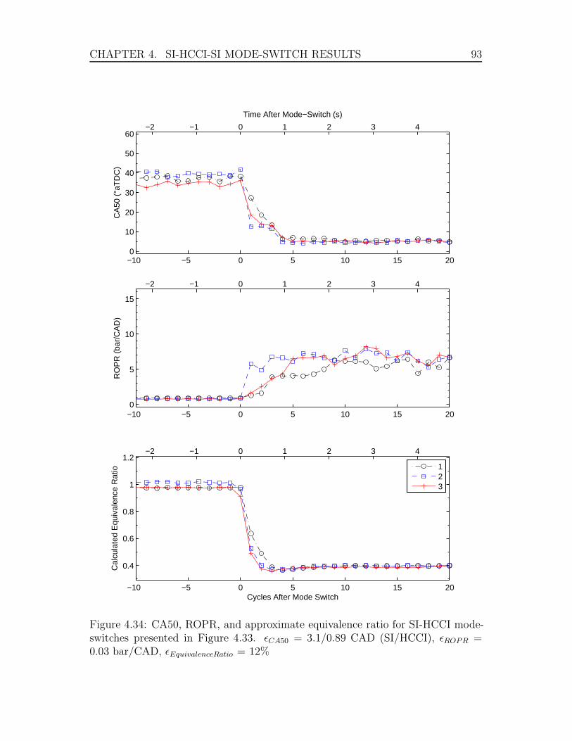
CHAPTER 4. SI-HCCI-SI MODE-SWITCH RESULTS 93
−10 −5 0 5 10 15 200
10
20
30
40
50
60
CA
50 (
°aT
DC
)−2 −1 0 1 2 3 4
Time After Mode−Switch (s)
−10 −5 0 5 10 15 200
5
10
15
RO
PR
(ba
r/C
AD
)
−2 −1 0 1 2 3 4
−10 −5 0 5 10 15 20
0.4
0.6
0.8
1
1.2
Cycles After Mode Switch
Cal
cula
ted
Equ
ival
ence
Rat
io
123
−2 −1 0 1 2 3 4
Figure 4.34: CA50, ROPR, and approximate equivalence ratio for SI-HCCI mode-switches presented in Figure 4.33. εCA50 = 3.1/0.89 CAD (SI/HCCI), εROPR =0.03 bar/CAD, εEquivalenceRatio = 12%
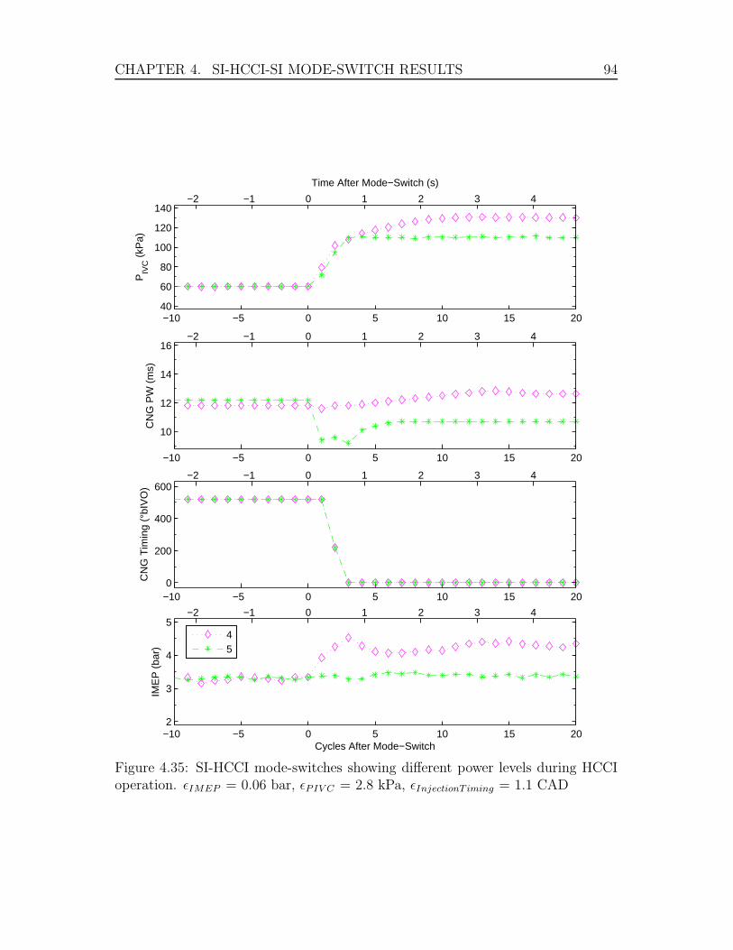
CHAPTER 4. SI-HCCI-SI MODE-SWITCH RESULTS 94
−10 −5 0 5 10 15 2040
60
80
100
120
140
PIV
C (
kPa)
−2 −1 0 1 2 3 4
Time After Mode−Switch (s)
−10 −5 0 5 10 15 20
10
12
14
16
CN
G P
W (
ms)
−2 −1 0 1 2 3 4
−10 −5 0 5 10 15 200
200
400
600
CN
G T
imin
g (°
bIV
O)
−2 −1 0 1 2 3 4
−10 −5 0 5 10 15 202
3
4
5
Cycles After Mode−Switch
IME
P (
bar)
45
−2 −1 0 1 2 3 4
Figure 4.35: SI-HCCI mode-switches showing different power levels during HCCIoperation. εIMEP = 0.06 bar, εPIV C = 2.8 kPa, εInjectionT iming = 1.1 CAD
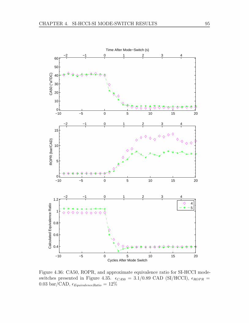
CHAPTER 4. SI-HCCI-SI MODE-SWITCH RESULTS 95
−10 −5 0 5 10 15 200
10
20
30
40
50
60
CA
50 (
°aT
DC
)−2 −1 0 1 2 3 4
Time After Mode−Switch (s)
−10 −5 0 5 10 15 200
5
10
15
RO
PR
(ba
r/C
AD
)
−2 −1 0 1 2 3 4
−10 −5 0 5 10 15 20
0.4
0.6
0.8
1
1.2
Cycles After Mode Switch
Cal
cula
ted
Equ
ival
ence
Rat
io
45
−2 −1 0 1 2 3 4
Figure 4.36: CA50, ROPR, and approximate equivalence ratio for SI-HCCI mode-switches presented in Figure 4.35. εCA50 = 3.1/0.89 CAD (SI/HCCI), εROPR =0.03 bar/CAD, εEquivalenceRatio = 12%
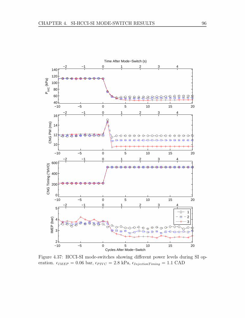
CHAPTER 4. SI-HCCI-SI MODE-SWITCH RESULTS 96
−10 −5 0 5 10 15 2040
60
80
100
120
140
PIV
C (
kPa)
−2 −1 0 1 2 3 4
Time After Mode−Switch (s)
−10 −5 0 5 10 15 20
10
12
14
16
CN
G P
W (
ms)
−2 −1 0 1 2 3 4
−10 −5 0 5 10 15 200
200
400
600
CN
G T
imin
g (°
bIV
O)
−2 −1 0 1 2 3 4
−10 −5 0 5 10 15 202
3
4
5
Cycles After Mode−Switch
IME
P (
bar)
123
−2 −1 0 1 2 3 4
Figure 4.37: HCCI-SI mode-switches showing different power levels during SI op-eration. εIMEP = 0.06 bar, εPIV C = 2.8 kPa, εInjectionT iming = 1.1 CAD
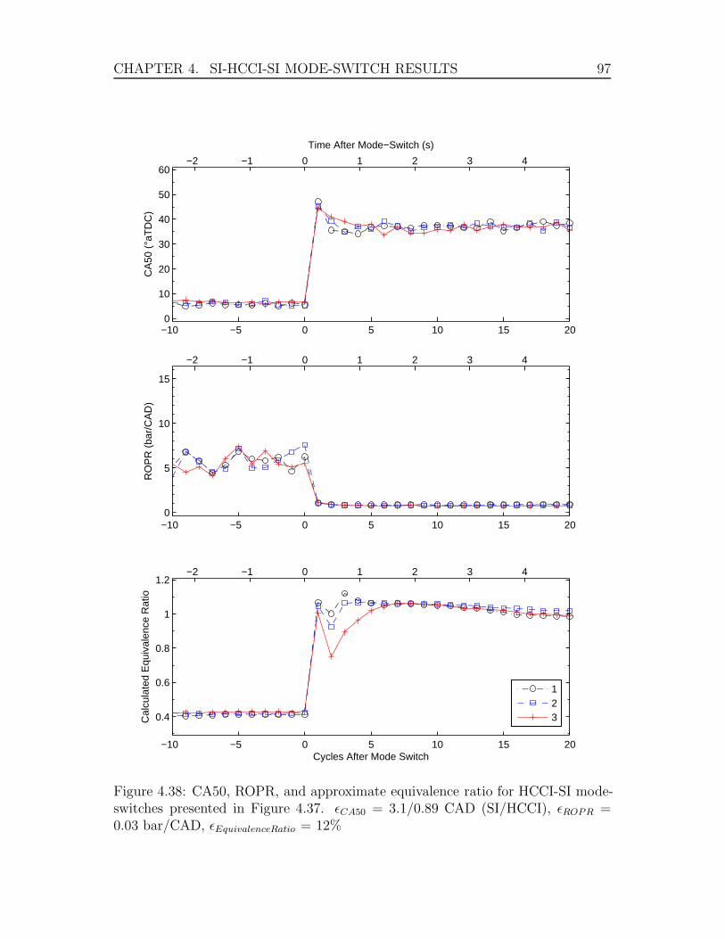
CHAPTER 4. SI-HCCI-SI MODE-SWITCH RESULTS 97
−10 −5 0 5 10 15 200
10
20
30
40
50
60
CA
50 (
°aT
DC
)−2 −1 0 1 2 3 4
Time After Mode−Switch (s)
−10 −5 0 5 10 15 200
5
10
15
RO
PR
(ba
r/C
AD
)
−2 −1 0 1 2 3 4
−10 −5 0 5 10 15 20
0.4
0.6
0.8
1
1.2
Cycles After Mode Switch
Cal
cula
ted
Equ
ival
ence
Rat
io
123
−2 −1 0 1 2 3 4
Figure 4.38: CA50, ROPR, and approximate equivalence ratio for HCCI-SI mode-switches presented in Figure 4.37. εCA50 = 3.1/0.89 CAD (SI/HCCI), εROPR =0.03 bar/CAD, εEquivalenceRatio = 12%
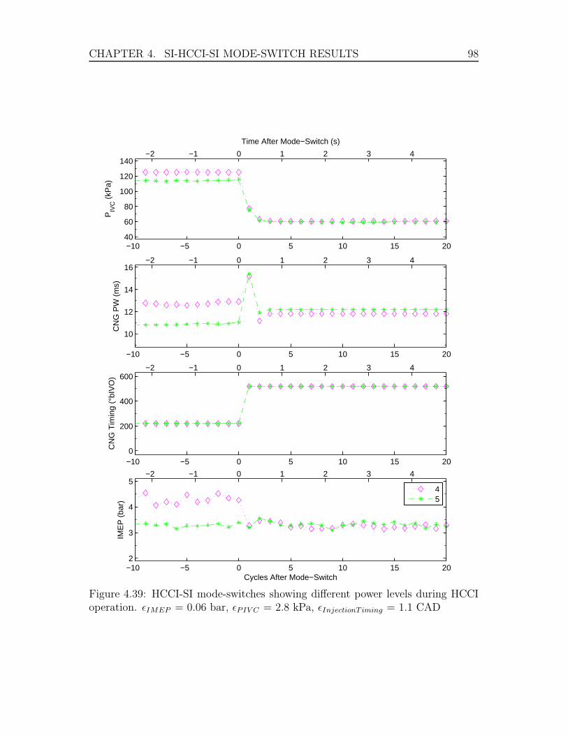
CHAPTER 4. SI-HCCI-SI MODE-SWITCH RESULTS 98
−10 −5 0 5 10 15 2040
60
80
100
120
140
PIV
C (
kPa)
−2 −1 0 1 2 3 4
Time After Mode−Switch (s)
−10 −5 0 5 10 15 20
10
12
14
16
CN
G P
W (
ms)
−2 −1 0 1 2 3 4
−10 −5 0 5 10 15 200
200
400
600
CN
G T
imin
g (°
bIV
O)
−2 −1 0 1 2 3 4
−10 −5 0 5 10 15 202
3
4
5
Cycles After Mode−Switch
IME
P (
bar)
45
−2 −1 0 1 2 3 4
Figure 4.39: HCCI-SI mode-switches showing different power levels during HCCIoperation. εIMEP = 0.06 bar, εPIV C = 2.8 kPa, εInjectionT iming = 1.1 CAD
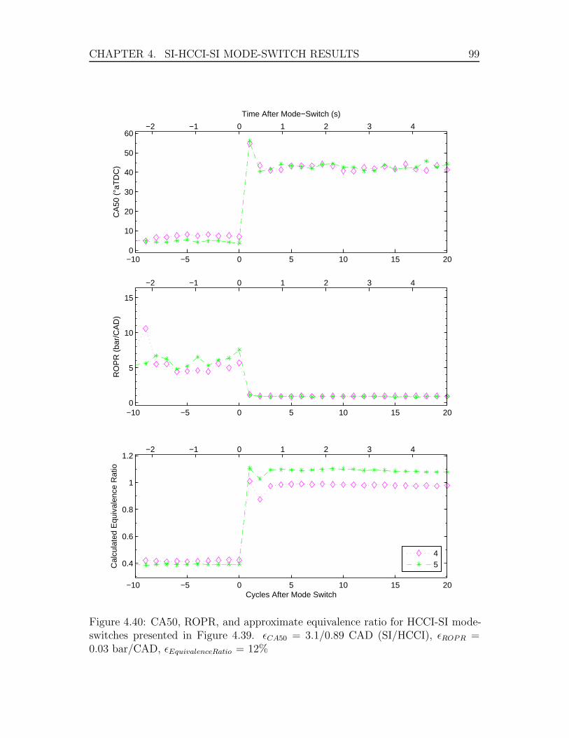
CHAPTER 4. SI-HCCI-SI MODE-SWITCH RESULTS 99
−10 −5 0 5 10 15 200
10
20
30
40
50
60
CA
50 (
°aT
DC
)−2 −1 0 1 2 3 4
Time After Mode−Switch (s)
−10 −5 0 5 10 15 200
5
10
15
RO
PR
(ba
r/C
AD
)
−2 −1 0 1 2 3 4
−10 −5 0 5 10 15 20
0.4
0.6
0.8
1
1.2
Cycles After Mode Switch
Cal
cula
ted
Equ
ival
ence
Rat
io
45
−2 −1 0 1 2 3 4
Figure 4.40: CA50, ROPR, and approximate equivalence ratio for HCCI-SI mode-switches presented in Figure 4.39. εCA50 = 3.1/0.89 CAD (SI/HCCI), εROPR =0.03 bar/CAD, εEquivalenceRatio = 12%
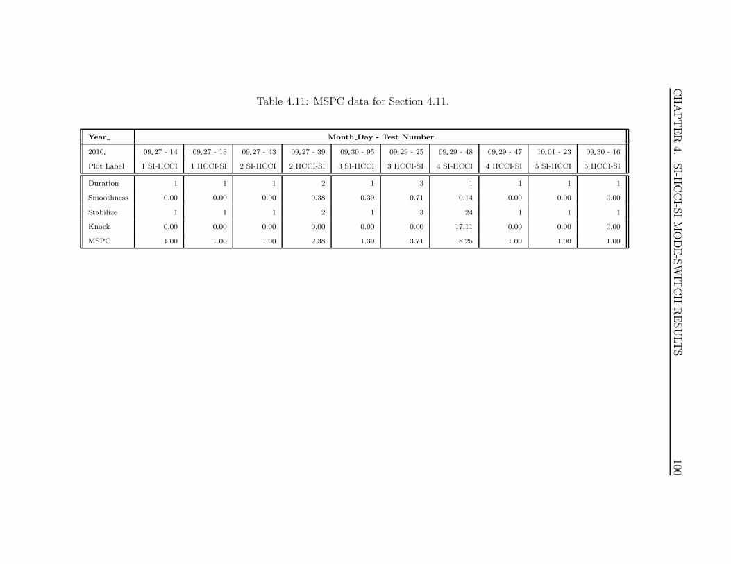
CHAPTER
4.SI-H
CCI-S
IMODE-SW
ITCH
RESULTS
100
Table 4.11: MSPC data for Section 4.11.
Year Month Day - Test Number
2010 09 27 - 14 09 27 - 13 09 27 - 43 09 27 - 39 09 30 - 95 09 29 - 25 09 29 - 48 09 29 - 47 10 01 - 23 09 30 - 16
Plot Label 1 SI-HCCI 1 HCCI-SI 2 SI-HCCI 2 HCCI-SI 3 SI-HCCI 3 HCCI-SI 4 SI-HCCI 4 HCCI-SI 5 SI-HCCI 5 HCCI-SI
Duration 1 1 1 2 1 3 1 1 1 1
Smoothness 0.00 0.00 0.00 0.38 0.39 0.71 0.14 0.00 0.00 0.00
Stabilize 1 1 1 2 1 3 24 1 1 1
Knock 0.00 0.00 0.00 0.00 0.00 0.00 17.11 0.00 0.00 0.00
MSPC 1.00 1.00 1.00 2.38 1.39 3.71 18.25 1.00 1.00 1.00

101
Chapter 5
Discussion
This chapter discusses the results presented in Chapter 4 for a better understanding
of engine response during SI-HCCI-SI mode-switching.
5.1 SI-HCCI-SI Mode-Switching With Conventional Actuators
Conventional actuators, throttle and CNG injection, are used in this study to
enable SI-HCCI mode-switching between two steady-state operating points. The
effects of adjusting these controls during a mode-switch are summarized in Figure
5.1. Higher P IVC resulting from larger throttle openings increases the tendency
toward knock, while lower P IVC increases the tendency toward misfire. CNG pulse
width has a similar response, while CNG injection timing promotes knock by more
advanced combustion timing. Achieving the desired IMEP for a smooth mode-
switch requires a balance between suitable combustion (no misfire or knock) and
the mass of CNG available during a combustion cycle for sufficient heat release.
For example, initial experiments in Section 4.2 avoid knock by reducing CNG PW,
but with an associated drop in IMEP; the later work in Section 4.8 achieves the
correct balance of actuators to avoid knock while still achieving the desired IMEP.
P IVC and CNG pulse width adjustments for HCCI-SI mode-switching follow a
similar response, as shown in Figure 5.2, with higher values having higher tendency

CHAPTER 5. DISCUSSION 102
−5 0 5 10 15 20 25 30
60
80
100
120
PIV
C (
kPa)
0 1 2 3 4 5
Time After Mode−Switch (s)
−5 0 5 10 15 20 25 30
9
9.5
10
10.5
11
11.5
12
CN
G P
W (
ms)
0 1 2 3 4 5
−5 0 5 10 15 20 25 300
100
200
300
400
500
600
Cycles After Mode−Switch
CN
G T
imin
g (°
bIV
O)
Knock TendencyMisfire Tendency
0 1 2 3 4 5
Figure 5.1: SI-HCCI mode-switching map showing actuator adjustments to tendtoward knock and misfire.
CHAPTER 5. DISCUSSION 103
toward knock. CNG timing, however, tends toward knock by retarding more slowly
over a greater number of cycles. These effects must be considered to avoid unex-
pected knock; however, mixture quality and spark timing during early SI operation
dictate IMEP and are controlled to achieve a smooth transition while avoiding mis-
fire. Leaner mixtures by reducing CNG PW at a given P IVC can be used to reduce
IMEP, but increase the likeliness of misfire; greater charge mass near stoichiometric
conditions increases IMEP with a higher tendency toward knock.
5.1.1 Redevelopment of Mode-Switching Control Sequences for An-
other Engine
The mode-switching strategies developed in this work provide a methodology to
develop open-loop control using only convention actuation for a candidate engine.
A more direct means of developing the control sequences is possible using experience
obtained from testing. These steps are outlined below.
First, compatible operating points must be found where stable operation in both
SI and HCCI combustion modes is possible with the same intake air temperature.
Tables 4.1, 4.6, and 4.10 indicate the operating points used in this study and may
be used for reference.
Throttle control values can be determined while motoring the engine without
fuel. The goal is to transition between the steady-state levels of P IVC and achieve
the same trend as demonstrated in Figures 4.22 or 4.26 depending on the direction
of mode-switch. P IVC values should be slightly lower than the steady-state values
determined above since CNG is not being injected in the intake manifold while
motoring. The amount lower can be determined by motoring the engine at the
same speed and throttle opening as the steady-state operating points found above
and measuring the reduced P IVC for both operating modes.
Develop the open-loop CNG injection parameters similar to the values in Fig-
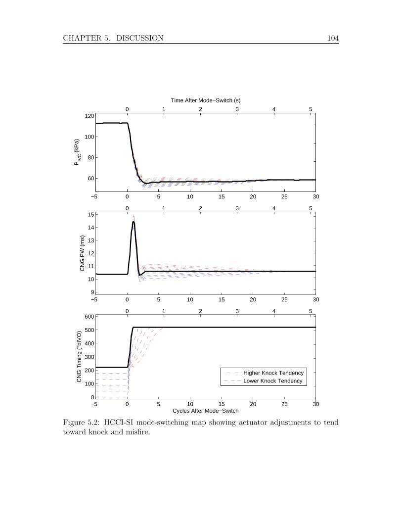
CHAPTER 5. DISCUSSION 104
−5 0 5 10 15 20 25 30
60
80
100
120
PIV
C (
kPa)
0 1 2 3 4 5
Time After Mode−Switch (s)
−5 0 5 10 15 20 25 309
10
11
12
13
14
15
CN
G P
W (
ms)
0 1 2 3 4 5
−5 0 5 10 15 20 25 300
100
200
300
400
500
600
Cycles After Mode−Switch
CN
G T
imin
g (°
bIV
O)
Higher Knock TendencyLower Knock Tendency
0 1 2 3 4 5
Figure 5.2: HCCI-SI mode-switching map showing actuator adjustments to tendtoward knock and misfire.
CHAPTER 5. DISCUSSION 105
ures 4.22 or 4.26 but scaled based on the new experimental setup (for instance, if
using a higher CNG injection pressure the pulse widths will have to be scaled down
to achieve a similar mass of CNG delivery per cycle). Reduce the mass delivered
for all cycles during and following the mode-switch by 10-20% to initially approach
misfire as opposed to knock.
Start the engine and operate in SI mode until steady-state (see Section 3.4)
is achieved at the desired mode-switch operating conditions. Attempt the mode-
switch using the developed throttle and fuel control sequences simultaneously. Note
that synchronization of input response on each cycle is essential. Increase fuel
delivery gradually on successive runs, starting with the early cycles in the mode-
switch, until IMEP and ROPR approach the target values. Figures 5.1 and 5.2 can
then be used to tune the control sequences and achieve the desired IMEP while
avoiding misfire and knock.
5.2 Repeated SI-HCCI-SI Mode-Switching
HCCI is sensitive to operational disturbances under normal operation, and this is
reflected in repeat mode-switches. ROPR following the first SI-HCCI transition,
shown in Figure 4.31, quickly approaches the target value of 6 bar/CAD since the
engine is under the intended conditions for mode-switching. Successive SI-HCCI
mode-switches experience a reduction in ROPR indicating reduced stability. Higher
variability in the IMEP results support this observation. Deviation increases as en-
gine conditions drift further from the steady-state values for which the mode-switch
sequence is developed. Even with degrading combustion, all mode-switches success-
fully achieve on-going HCCI operation. CA50 approaches the steady-state value
quickly following all SI-HCCI mode-switches, taking only 2-3 cycles to transition.
Based on this test, the open-loop control being implemented can handle some
level of disturbance while still completing the mode-switch properly. Further devi-
CHAPTER 5. DISCUSSION 106
ation from the design conditions would eventually lead to misfire or knock, which
could be addressed with some form of feedback or adaptive control. Profiling addi-
tional operating points to map a range of expected conditions may also provide a
means of adapting to disturbances through interpolation [34]. Additional consider-
ation of environmental conditions (air temperature, humidity, etc.) and operating
variables (fuel composition, oil temperature, etc.) will require further investigation
to determine their influence on mode-switching and the degree of control necessary
to accommodate them.
5.3 Variation in Steady-State IMEP for SI-HCCI Mode-Switching
In Figures 4.33 and 4.35, the CNG PW is commanded to respond in a manner
proportional to the difference in steady-state IMEP levels. Having a small IMEP
increase from SI to HCCI suggests that lower values of CNG PW are needed during
the initial HCCI cycles. This is likely due to the relatively hotter residual gases and
combustion chamber surfaces, promoting earlier ignition timing and more efficient
combustion.
Similarly in Figure 4.33, intake pressure must be increased at a faster rate when
starting at a lower IMEP level in SI and stepping up to the same IMEP in HCCI.
The calculated equivalence ratios in Figure 4.34 show an obvious trend with the
first three cycles corresponding to the differences in fuel and intake pressure as
discussed above, with all tests approaching the same steady-state level as HCCI
combustion stabilizes.
Observing IMEP data for SI-HCCI transitions in Figures 4.33 and 4.35, it is
evident that the third cycle after the mode-switch shows a sudden increase for
most tests. This is related to advancing CNG injection timing directly to IVO
causing combustion timing to advance. The sudden decrease in fuel on this cycle
for test 3 in Figure 4.33 is an attempt to counteract this effect; however, it appears
CHAPTER 5. DISCUSSION 107
that a greater reduction in CNG PW is necessary. Test 5 in Figure 4.35 uses a
more significant reduction in fuel for this cycle, successfully removing the IMEP
increase for a smoother transition. An alternative approach could be to advance
the injection timing more slowly at this cycle, which as discussed in Chapter 3 is a
limitation of this experimental setup.
SI-HCCI mode-switching to higher levels of IMEP in HCCI are found to be more
prone to knock, as demonstrated by test 4 in Figure 4.36. Further tuning of this
point may remove this condition by increasing intake pressure at a slower rate, or by
overcoming the injection timing limitation and advancing the injection event toward
IVO at a slower rate than the 2 cycle step implemented here. Leaner mixtures
by reducing CNG mass delivery during the knock period could also remedy the
situation, but likely at the expense of a longer transition to the steady-state IMEP
in HCCI. Addition of external EGR could also be employed to mitigate knock in
this scenario, but with careful consideration necessary due to the significant change
in exhaust gas flow rate, temperature, and composition during the mode-switch.
Another alternative would be to reduce the engine compression ratio to achieve
higher IMEP in HCCI through greater supercharging pressure [23]; however, for
a conventionally controlled engine, this adjustment would not be possible during
operation and would be restricted to an initial design decision.
5.4 Variation in Steady-State IMEP for HCCI-SI Mode-Switching
For mode-switching from HCCI to SI, most notable for discussion is the fuel delivery
during early SI operation. CNG PW must be increased significantly on the first
SI cycle, as demonstrated in Figures 4.37 and 4.39, to allow SI ignition with the
greater air mass. The objective is to keep the mixture stoichiometric or slightly
lean to avoid an increase in IMEP by retarding combustion past the steady-state
CA50 value. Calculated equivalence ratios in Figures 4.38 and 4.40 suggest that
CHAPTER 5. DISCUSSION 108
near stoichiometric conditions are experienced during this first SI cycle, with the
exception of test 5 that appears to be running slightly rich and yet still exhibits
a similarly late CA50. Ongoing rich mixtures are calculated for SI in test 5 as
operation stabilizes. Comparing these with the equivalence ratio provided in Table
4.10, which instead is derived from average mass flow measurements of air and
CNG, the rich tendency shown in Figure 4.40 is believed to be an artifact of the
per-cycle equivalence ratio calculations outlined in Section 3.1.4. The higher intake
air temperature is the likely cause for the deviation. Note that the 12% error in
this parameter still includes stoichiometric operation for these cycles.
Moving forward, the second SI cycle in Figures 4.37 and 4.39 following an
HCCI-SI mode-switch reduces CNG PW to slightly below the steady-state level
for smoother IMEP response. All following cycles are held at the steady-state
level. In all tests, there are some fluctuations in the calculated equivalence ratio
during cycles 2-4, shown in Figures 4.38 and 4.40, as P IVC and other conditions
stabilize. A more consistent equivalence ratio during early SI operation could be
achieved by tailoring the inputs based on these results, although the smoothness of
IMEP and the other calculated parameters suggest that re-testing would provide
little visible benefit. Only test 3 shows a significant deviation from stoichiometric
operation, where leaner mixtures during cycles 2-4 help reduce IMEP more quickly
as the intake pressure continues to decrease to the desired steady-state level. CA50
data in Figure 4.38 supports this with a smoother yet longer transition toward
steady-state ignition timing.
Test 5 in Figures 4.35 and 4.39 presents a constant load mode-switch that is
useful for applications where it is desirable to achieve HCCI combustion without
disturbing power output. A higher intake temperature is necessary under the
conditions tested in order to reduce HCCI power sufficiently for this purpose, as
IMEP in SI could not be increased without experiencing knock at these high intake
CHAPTER 5. DISCUSSION 109
temperatures. This demonstrates the potential limits in the ability of the engine
to respond to a broad range of power requirements at the mode-switch boundary
using only fast conventional actuators. On the other hand, it is interesting to know
that a constant load SI-HCCI-SI mode-switch is possible using only conventional
actuation.
5.5 Mode-Switching Performance Criterion (MSPC)
The performance of this parameter is explored by evaluating all of the mode-
switching done in this study and comparing the results qualitatively relative to
one another, as is the current standard procedure. Individual components (du-
ration, smoothness, and knock) and the overall average and standard deviation
of each set of data correlates well with the subjective observations regarding the
different methods.
Subjective observations for each section correlate well with the the individual
components of MSPC (duration, smoothness, and knock) as well as the overall
average and standard deviation for the 10 tests in each set.
For instance, Section 4.2 provided a rough modes-switch with a large drop in
IMEP for several cycles, but is fairly repeatable; whereas Section 4.3 is generally a
better switch but with more variability between tests with some containing partial
burn or knock cycles. Correspondingly, Section 4.2 provides a much higher aver-
age MSPC than Section 4.3, but with a lower standard deviation between tests.
Other sections compare similarly with the qualitative discussion presented in the
associated sections. Values follow the expected trend with less refined tests from
the earlier sections providing much higher (less desirable) MSPC values than the
optimized scenarios.
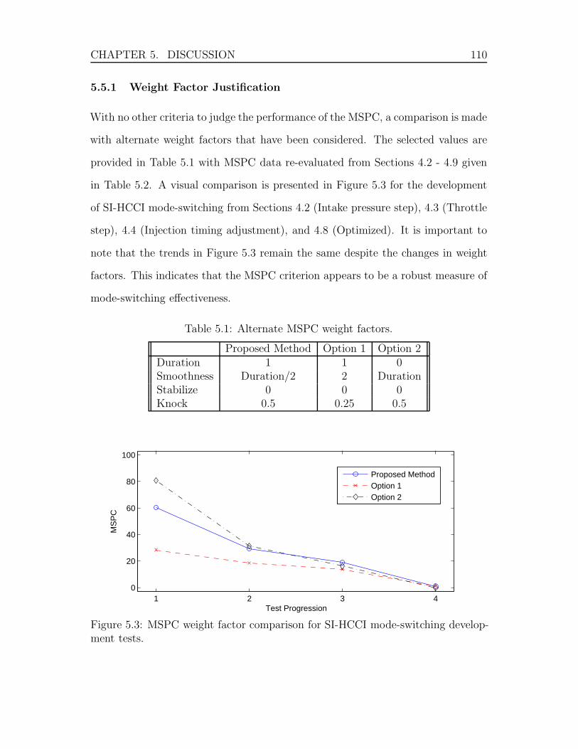
CHAPTER 5. DISCUSSION 110
5.5.1 Weight Factor Justification
With no other criteria to judge the performance of the MSPC, a comparison is made
with alternate weight factors that have been considered. The selected values are
provided in Table 5.1 with MSPC data re-evaluated from Sections 4.2 - 4.9 given
in Table 5.2. A visual comparison is presented in Figure 5.3 for the development
of SI-HCCI mode-switching from Sections 4.2 (Intake pressure step), 4.3 (Throttle
step), 4.4 (Injection timing adjustment), and 4.8 (Optimized). It is important to
note that the trends in Figure 5.3 remain the same despite the changes in weight
factors. This indicates that the MSPC criterion appears to be a robust measure of
mode-switching effectiveness.
Table 5.1: Alternate MSPC weight factors.
Proposed Method Option 1 Option 2Duration 1 1 0Smoothness Duration/2 2 DurationStabilize 0 0 0Knock 0.5 0.25 0.5
1 2 3 40
20
40
60
80
100
Test Progression
MS
PC
Proposed MethodOption 1Option 2
Figure 5.3: MSPC weight factor comparison for SI-HCCI mode-switching develop-ment tests.
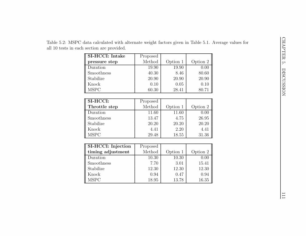
CHAPTER
5.DISCUSSIO
N111
Table 5.2: MSPC data calculated with alternate weight factors given in Table 5.1. Average values forall 10 tests in each section are provided.
SI-HCCI: Intake Proposedpressure step Method Option 1 Option 2Duration 19.90 19.90 0.00Smoothness 40.30 8.46 80.60Stabilize 20.90 20.90 20.90Knock 0.10 0.05 0.10MSPC 60.30 28.41 80.71
SI-HCCI: ProposedThrottle step Method Option 1 Option 2Duration 11.60 11.60 0.00Smoothness 13.47 4.75 26.95Stabilize 20.20 20.20 20.20Knock 4.41 2.20 4.41MSPC 29.48 18.55 31.36
SI-HCCI: Injection Proposedtiming adjustment Method Option 1 Option 2Duration 10.30 10.30 0.00Smoothness 7.70 3.01 15.41Stabilize 12.30 12.30 12.30Knock 0.94 0.47 0.94MSPC 18.95 13.78 16.35
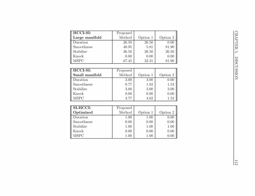
CHAPTER
5.DISCUSSIO
N112
HCCI-SI: ProposedLarge manifold Method Option 1 Option 2Duration 26.50 26.50 0.00Smoothness 40.95 5.81 81.90Stabilize 26.50 26.50 26.50Knock 0.00 0.00 0.00MSPC 67.45 32.31 81.90
HCCI-SI: ProposedSmall manifold Method Option 1 Option 2Duration 3.00 3.00 0.00Smoothness 0.77 1.02 1.53Stabilize 3.00 3.00 3.00Knock 0.00 0.00 0.00MSPC 3.77 4.02 1.53
SI-HCCI: ProposedOptimized Method Option 1 Option 2Duration 1.00 1.00 0.00Smoothness 0.00 0.00 0.00Stabilize 1.00 1.00 1.00Knock 0.00 0.00 0.00MSPC 1.00 1.00 0.00
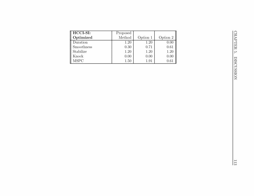
CHAPTER
5.DISCUSSIO
N113
HCCI-SI: ProposedOptimized Method Option 1 Option 2Duration 1.20 1.20 0.00Smoothness 0.30 0.71 0.61Stabilize 1.20 1.20 1.20Knock 0.00 0.00 0.00MSPC 1.50 1.91 0.61
CHAPTER 5. DISCUSSION 114
5.5.1.1 Option 1
Smoothness in this alternative is weighted with a constant value that is not depen-
dent on the duration. The drawback of this approach is most notable in Figure
5.3 where only a small difference exists between the first two SI-HCCI tests, intake
pressure step and throttle step. Experimental observations of IMEP data from the
intake pressure step tests experienced a significant drop for early HCCI cycles that
was eliminated in the following throttle step tests. The proposed method more ac-
curately demonstrates this improvement with its duration-dependent weight factor
for smoothness.
The knock penalty is also reduced in this alternative by one half. The result is
that all knock values scale down by a factor of 2 for a similar relative influence on
the final MSPC as in the proposed method. The linear relationship between knock
intensity and ROPR has been assumed for the evaluation of MSPC and can not be
verified further without a detailed investigation.
5.5.1.2 Option 2
Another method to evaluate mode-switch performance is to consider duration only
as the weight factor for smoothness. The improvement in IMEP smoothness be-
tween the intake pressure step and throttle step tests is accurately represented by
MSPC, as demonstrated in Figure 5.3. For the tests presented in Table 5.2, it is
not evident why this option is less desirable than the proposed method, but can be
discussed in a theoretical sense.
The objective of mode-switching is to achieve the new steady-state IMEP level
in a quick and smooth manner. The developed smoothness criterion only evaluates
deviation from a linear trend between the initial and final IMEP levels with no
direct indication of the number of cycles involved in this calculation. In the case
where the engine responds very close to this linear trend and COV IMEP trans is less
CHAPTER 5. DISCUSSION 115
than 5%, smoothness is assigned a value of 0 and the duration weight factor has
no effect. This case should only be considered ideal if the linear trend occurs over
a single cycle as well, or the requirement for a “quick” mode-switch has not been
met. The proposed method takes this into account by considering an independent
duration penalty.
5.5.2 Extension of MSPC to Other Scenarios
As presented thus far, MSPC is useful for evaluating mode-switching on a single-
cylinder engine between two arbitrary IMEP levels. Moving toward real-world
applications, other issues arise requiring attention: transition of slow actuators,
power demand, and multiple cylinders. With minor modifications, the MSPC can
cover these scenarios as well.
5.5.2.1 Power Demand
Adapting MSPC to a dynamic power demand is easily accomplished. Instead of
finding the steady-state IMEP in the final combustion mode, the target values con-
sist of the demand for the engine as it is being controlled. Equations 3.10, 3.11, and
3.12 still apply and the mode-switch is considered complete when COVIMEP trans,
comprised of a running 15 cycles, drops below 5%. This scenario will become more
prominent as mode-switching controllers are developed and performance must be
evaluated while responding to an unknown input from an operator.
5.5.2.2 Transition of Slow Actuators
Mode-switching is evaluated between two steady-state points in this study with nei-
ther representing typical operation in either SI or HCCI. Under normal operation,
the engine will be required to transition slow actuators, such as intake tempera-
ture, to a region able to support a mode-switch, initiate the mode-switch itself,
CHAPTER 5. DISCUSSION 116
then transition to the final operating point. Engine operation during these slow
transitions may or may not require a penalty depending on whether the engine can
respond to demand.
The variable power demand discussed above can be evaluated during this tran-
sition with any deviation from the target IMEP causing a COVIMEP trans greater
than 5% or knock cycles leading to penalties similar to during the mode-switch
itself. If IMEP deviation and knock reduce to an acceptable level before the en-
tire transition is complete, penalties will not be necessary until the mode-switch
itself or the engine deviates again. This incorporates the benefit of mode-switching
strategies incorporating more comprehensive actuators, such as variable valve tech-
nology, that can adjust cylinder conditions sufficiently with all fast actuators and
avoid transition time of any slow actuators. On the other hand, applications where
power demand does not change instantaneously or can be predicted may not need
the capibility to mode-switch without slow actuation first, and may benefit more
from a mechanically simpler solution.
For this study, slow actuation is not tested or considered. The engine operates
steady-state in both modes at the selected operating conditions, so a transition of
slow actuators is unnecessary. Intake air temperature responds with a very long
time constant in the existing setup, so the feasibility of repeating mode-switches
for development is further time limited. Modifications could be made to improve
response time by installing an electric air heater or exhaust gas heat exchanger with
improved air contact surface area and reduced thermal mass, or by implementing
a fast thermal management system (mixing air from hot and cold streams). This
would allow for investigation of the transition between mode-switching operating
conditions and more typical operating points for SI and HCCI.
CHAPTER 5. DISCUSSION 117
5.5.2.3 Multiple Cylinders
Mode-switching with multiple cylinders adds the complication of deciding how to
combine the data in a representative and suitable manner. A few alternatives are
considered:� First, averaging the data (IMEP and ROPR) from all cylinders on each cycle
provides an indication of overall engine performance during the mode-switch.
Analysis is simple and can be carried out in the same manner as presented;
however, misfire, partial burn, and knock cycles may occur on individual cylin-
ders simultaneously, with the averaging causing the stability of the engine to
be mis-represented.� Another approach is to consider each combustion event sequentially across
all cylinders. Cycles with poor combustion are evaluated properly, but the
duration and smoothness of the mode-switch analysis may be compromised
if certain cylinders take longer to stabilize than others.� Finally, each cylinder could be considered individually and evaluated as pre-
sented in this study. Cylinders may progress through the mode-switch at
different rates based on operating conditions and the control scheme being
used, and each cylinder would also account for undesirable knock or misfire.
The last option offers the most representative evaluation and is discussed fur-
ther. For example, assume that all tests in one of the mode-switching development
sections in Chapter 4 are individual cylinders in a 10-cylinder engine. The average
MSPC would describe the engine’s overall mode-switch performance for that sin-
gle test, while the standard deviation of MSPC represents the variability between
cylinders for the same test. The only necessary adaptation to the presented defini-
tion of MPSC is a method to combine results from several tests in a representative
manner of performance and repeatability:
CHAPTER 5. DISCUSSION 118� The average MSPC for each test (MSPCi) could be combined to provide the
overall performance of the mode-switching method (µMSPC).� The standard deviation between MSPCi evaluates the stability of the mode-
switching method for the engine as a whole (σMSPC).� Averaging the standard deviation of MSPC between cylinders for each test
represents the typical variability between cylinders (σMSPC cyl).
Together, these three values should provide a good indication of the overall
performance of a mode-switching strategy on a multiple-cylinder engine. Written
expressions for these definitions are summarized here:
µMSPC =1
J
J∑
i=1
MSPCi (5.1a)
σMSPC =
√
√
√
√
1
J
J∑
i=1
(MSPCi − µMSPC)2 (5.1b)
σMSPC cyl =1
J
J∑
i=1
√
√
√
√
1
M
M∑
j=1
(MSPCcyl(j) −MSPCi)2 (5.1c)
J = Number of Tests
M = Number of Cylinders
119
Chapter 6
Conclusions
The objective of this study is to investigate SI-HCCI-SI mode-switching through
conventional actuation and establish a means of quantitatively evaluating mode-
switching performance. Accomplishments are summarized in the following sections.
Potential avenues to further this strategy of mode-switching are also presented.
6.1 SI-HCCI-SI Mode-Switching Through Conventional Actuation
A modified CFR engine operating with port-injected CNG is utilized to explore
SI-HCCI-SI mode-switching with conventional actuation. Late spark timing and
throttling are implemented to avoid knock during SI with heated intake air. Testing
explores the influence of intake pressure, CNG injection mass, and CNG injection
timing on mode-switching between SI and HCCI in both directions. Slow actuators
such as intake air temperature are not adjusted during the transition. The large
intake manifold fitted on the engine initially is determined to be a limiting factor
and reduced from 10L to approximately one engine displacement, or 0.5 L, to
increase control over air delivery.
Open-loop control is developed experimentally for each sequence of actuator
inputs used to mode-switch. Repeatability is explored during development by run-
ning open-loop sequences 10 times under the same conditions. Optimized scenar-

CHAPTER 6. CONCLUSIONS 120
ios for mode-switching in both directions are achieved where the new steady-state
IMEP is achieved within 1 engine cycle and maintained.
Sensitivities to disturbances are explored by quickly repeating several mode-
switches over a one minute period using the same open-loop control sequences as
developed for steady-state conditions. Stability in HCCI following an SI-HCCI
mode-switch is reduced later in the sequence, but still successfully achieves HCCI
combustion in a quick and relatively smooth manner without knock or misfire. In
some instances, the first SI cycle following an HCCI-SI mode-switch experiences
partial combustion due to the slightly lean mixtures used to limit IMEP. More
fuel on this cycle could correct the issue by potentially adding one cycle to the
transition duration at an intermediate IMEP.
Initial profiling of the mode-switching region is carried out under various con-
ditions at a slower engine speed of 500 RPM. A range of IMEP is demonstrated in
both SI and HCCI steady-state regions surrounding a mode-switch with modified
open-loop control sequences achieving relatively smooth transitions in both direc-
tions. This proves that mode-switching using conventional actuation is possible at
more than a single operating point.
6.2 Mode-Switching Performance Criterion (MSPC)
Mode-switching is evaluated using the developed quantitative measure of duration,
smoothness, and knock. This single value, MSPC, can describe the overall effective-
ness of a mode-switch under any means of actuation. Comparing with qualitative
observation, the current standard, MSPC and its components correlate very well
with experimental data in this study. Adaptation of MSPC analysis for situations
with variable power demand, necessary transitions of slow actuators, and multiple-
cylinder engines is forecast to require only minor adjustments beyond the method
presented.
CHAPTER 6. CONCLUSIONS 121
6.3 Future Work
Several possibilities exist as potential areas of research to further develop these two
topics:� Test the influence of other common actuators for their ability to assist and
control combustion during a mode-switch. Some possibilities include variable
spark timing and exhaust back pressure (such as from a turbocharger). Exter-
nal EGR is commonly used to stabilize HCCI operation and reduce emissions,
but offers complications due to variable exhaust composition, temperature,
and mass flow during the mode-switch that will have to be accounted for.� Valve timing more suitable to HCCI operation may be desirable for an engine
designed to operate primarily in HCCI, but potential for knock during SI op-
eration will have to be explored. Compression ratio may also be adjusted to
shift operating conditions for mode-switching based on the relationship be-
tween intake temperature, boost pressure, and heat rise during compression.� Profile the range of possible mode-switching points for different engine speeds,
power levels, and states of slow actuators. A method to determine mode-
switching control sequences at intermediate operating points may be possible
similar to [34], or model-based controllers capable of adapting to measurable
engine conditions and disturbances could be developed. Detailed modeling
of the mode-switching with conventional actuators would improve the under-
standing of conditions necessary to achieve the desired combustion, making
controller design more robust and comprehensive.� Adapt this mode-switching method to multi-cylinder operation. Since indi-
vidual throttle control for each cylinder is unlikely due to cost and complexity,
a range of intake pressures will be experienced during transition through the

CHAPTER 6. CONCLUSIONS 122
unstable region between combustion modes. Other actuators will have to be
adjusted to maintain suitable combustion.� Evaluating COV IMEP over a limited number of engine cycles for MSPC could
be explored in greater detail to validate that 15 cycles represents a suitable
approximation of engine stability defining the end of a mode-switch.� Apply MSPC evaluation to mode-switching data from a multiple cylinder
engine to validate the proposed summary parameters.
123
Bibliography
[1] John B. Heywood. Internal Combustion Engine Fundamentals. McGraw-Hill,
Inc., 1988.
[2] Hua Zhao, editor. HCCI and CAI engines for the automotive industry. Wood-
head Publishing Limited, 2007.
[3] Shigeru Onishi, Souk Hong Jo, Katsuji Shoda, Pan Do Jo, and Satoshi Kato.
Active Thermo-Atmosphere Combustion (ATAC) - A New Combustion Pro-
cess For Internal Combustion Engines. SAE Technical Paper Series, 790501.
[4] Paitoon Kongsereeparp. Chemical Kinetic Based Simulation for an HCCI
Engine and its Combustion. PhD thesis, University of Alberta, 2008.
[5] Paitoon Kongsereeparp and David Checkel. Study of Reformer Gas Effects on
n-Heptane HCCI Combustion Using a Chemical Kinetic Mechanism Optimized
by Genetic Algorithm. SAE Technical Paper Series, 2008-01-0039.
[6] Mingfa Yao, Zhaolei Zheng, and Haifeng Liu. Progress and Recent Trends
in Homogeneous Charge Compression Ignition (HCCI) Engines. Progress in
Energy and Combustion Science, 35(5):398 – 437, 2009.
[7] Junseok Chang, Orgun Gralp, Zoran Filipi, Dennis Assanis, Tang-Wei Kuo,
Paul Najt, and Rod Rask. New Heat Transfer Correlation for an HCCI En-
gine Derived from Measurements of Instantaneous Surface Heat Flux. SAE
Technical Paper Series, 2004-01-2996.
BIBLIOGRAPHY 124
[8] Jessica Marshall. Clean-burn engine dodges ever tighter regulations. New
Scientist, 189(2534):26 – 27, 2006.
[9] Hailin Li, W. Stuart Neill, Wally Chippior, Lisa Graham, Trevor Connolly,
and Joshua D. Taylor. An Experimental Investigation on the Emission Char-
acteristics of HCCI Engine Operation Using N-Heptane. SAE Technical Paper
Series, 2007-01-1854.
[10] Rudolf H. Stanglmaier, Thomas W. Ryan III, and Jason S. Souder. HCCI
Operation of a Dual-Fuel Natural Gas Engine for Improved Fuel Efficiency and
Ultra-Low NOx Emissions at Low to Moderate Engine Loads. SAE Technical
Paper Series, 2001-01-1897.
[11] Mahdi Shahbakhti and Charles Robert Koch. Physics Based Control Oriented
Model for HCCI Combustion Timing. Journal of Dynamic Systems, Measure-
ment and Control, Transactions of the ASME, 132:021010, 1–12, 2010.
[12] Adrian D. Audet. Closed Loop Control of HCCI using Camshaft Phasing and
Dual Fuels. Master’s thesis, University of Alberta, 2008.
[13] J. Bengtsson, P. Strandh, R. Johansson, P. Tunestl, and B. Johansson. Hy-
brid modelling of homogeneous charge compression ignition (HCCI) engine
dynamics - A survey. International Journal of Control, 80(11):1814 – 1848,
2007.
[14] Robert Anthony William Lupul. Steady State and Transient Characterization
of a HCCI Engine with Varying Octane Fuel. Master’s thesis, University of
Alberta, 2008.
[15] Zhi Wang, Jian-Xin Wang, Guo hong Tian, Shi-Jin Shuai, Zhifu Zhang, and
Junwei Yang. Research on Steady and Transient Performance of an HCCI
BIBLIOGRAPHY 125
Engine with Gasoline Direct Injection. SAE Technical Paper Series, 2008-01-
1723.
[16] Vahid Hosseini. Reformer Gas Application in HCCI Combustion Engine. PhD
thesis, University of Alberta, 2008.
[17] Daniel L. Flowers, Nick J. Killingsworth, Francisco Espinosa-Loza, Joel
Martinez-Frias, Salvador M. Aceves, Miroslav Krstic, and Robert Dibble.
Demonstrating Optimum HCCI Combustion with Advanced Control Technol-
ogy. SAE Technical Paper Series, 2009-01-1885.
[18] Gran Haraldsson, Jari Hyvonen, Per Tunestl, and Bengt Johansson. HCCI
Closed-Loop Combustion Control Using Fast Thermal Management. SAE
Technical Paper Series, 2004-01-0943. Collection.
[19] Daniel I. Handford. Direct Injection Assisted HCCI Combustion of Natural
Gas. Master’s thesis, University of Alberta, 2009.
[20] Adrian Audet and Charles Robert Koch. Actuator comparison for closed loop
control of HCCI combustion timing. SAE Technical Paper Series, 2009-01-
1135.
[21] Sotirios Mamalis, Vishnu Nair, Peter Andruskiewicz, Dennis Assanis, Aris-
totelis Babajimopoulos, Nicole Wermuth, and Paul Najt. Comparison of Dif-
ferent Boosting Strategies for Homogeneous Charge Compression Ignition En-
gines - A Modeling Study. SAE Technical Paper Series, 2010-01-0571.
[22] D. I. Handford and M. D. Checkel. Extending the Load Range of a Natural
Gas HCCI Engine using Direct Injected Pilot Charge and External EGR. SAE
Technical Paper Series, 2009-01-1884.
BIBLIOGRAPHY 126
[23] Yuuichi Kodama, Izumi Nishizawa, Takumi Sugihara, Norihiko Sato, Tadashi
Iijima, and Tatsuya Yoshida. Full-Load HCCI Operation with Variable Valve
Actuation System in a Heavy-Duty Diesel Engine. SAE Technical Paper Series,
2007-01-0215.
[24] Hiroshi Kuzuyama, Masahiro Machida, Kazuhiro Akihama, Kazuhisa Inagaki,
and Matsuei Ueda. A Study on Natural Gas Fueled Homogeneous Charge
Compression Ignition Engine - Expanding the Operating Range and Combus-
tion Mode Switching. SAE Technical Paper Series, 2007-01-0176.
[25] Wen Zeng and Maozhao Xie. A novel approach to reduce hydrocarbon emis-
sions from the HCCI engine. Chemical Engineering Journal, 139(2):380 – 389,
2008.
[26] ShazamWilliams, Linjie (Robin) Hu, Tohru Nakazono, Hiroyuki Ohtsubo, and
Miwa Uchida. Oxidation Catalysts for Natural Gas Engine Operating under
HCCI or SI Conditions. SAE Technical Paper Series, 2008-01-0807.
[27] Magnus Christensen, Bengt Johansson, and Patrik Einewall. Homogeneous
Charge Compression Ignition (HCCI) Using Isooctane, Ethanol and Natural
Gas - A Comparison with Spark Ignition Operation. SAE Technical Paper
Series, 972874.
[28] Joel Hiltner, Scott Fiveland, Rey Agama, and Martin Willi. System Efficiency
Issues for Natural Gas Fueled HCCI Engines in Heavy-Duty Stationary Appli-
cations. SAE Technical Paper Series, 2002-01-0417.
[29] Jim Iverson. EPA emissions regulations: What they mean for standby, prime
and distributed power systems. Technical report, Cummings Power Genera-
tion, 2006.
BIBLIOGRAPHY 127
[30] H. M. Cho and B.-Q. He. Combustion and Emission Characteristics of a Lean
Burn Natural Gas Engine. International Journal of Automotive Technology,
9(4):415–422, 2008.
[31] Patrik Einewall, Per Tunestl, and Bengt Johansson. Lean Burn Natural Gas
Operation vs. Stoichiometric Operation with EGR and a Three Way Catalyst.
SAE Technical Paper Series, 2005-01-0250.
[32] Ruonan Sun, Rick Thomas, and Charles L. Gray Jr. An HCCI Engine: Power
Plant for a Hybrid Vehicle. SAE Technical Paper Series, 2004-01-0933.
[33] Alasdair Cairns and Hugh Blaxill. The Effects of Two-Stage Cam Profile
Switching and External EGR on SI-CAI Combustion Transitions. SAE Tech-
nical Paper Series, 2007-01-0187.
[34] Jonathan Etheridge, Sebastian Mosbach, Markus Kraft, Hao Wu, and Nick
Collings. A Fast Detailed-Chemistry Modelling Approach for Simulating the
SI-HCCI Transition. SAE Technical Paper Series, 2010-01-1241.
[35] Guohong Tian, Zhi Wang, Qiangqing Ge, Jianxin Wang, and Shijin Shuai.
Mode Switch of SI-HCCI Combustion on a GDI Engine. SAE Technical Paper
Series, 2007-01-0195.
[36] Hiromu Kakuya, Shiro Yamaoka, Kengo Kumano, and Shinya Sato. Investiga-
tion of a SI-HCCI Combustion Switching Control Method in a Multi-Cylinder
Gasoline Engine. SAE Technical Paper Series, 2008-01-0792.
[37] Nebojsa Milovanovic, Dave Blundell, Stephen Gedge, and Jamie Turner. SI-
HCCI-SI Mode Transition at Different Engine Operating Conditions. SAE
Technical Paper Series, 2005-01-0156.
BIBLIOGRAPHY 128
[38] Nebojsa Milovanovic, Dave Blundell, Stephen Gedge, and Jamie Turner. Cam
Profile Switching (CPS) and Phasing Strategy vs Fully Variable Valve Train
(FVVT) Strategy for Transitions between Spark Ignition and Controlled Auto
Ignition Modes. SAE Technical Paper Series, 2005-01-0766.
[39] Hao Wu, Nick Collings, Simon Regitz, Jonathan Etheridge, and Markus Kraft.
Experimental Investigation of a Control Method for SI-HCCI-SI Transition in
a Multi-Cylinder Gasoline Engine. SAE Technical Paper Series, 2010-01-1245.
[40] Yan Zhang, Hui Xie, and Hua Zhao. Investigation of SI-HCCI Hybrid Combus-
tion and Control Strategies for Combustion Mode Switching in a Four-stroke
Gasoline Engine. Combustion Science and Technology, 181:782–799, 2009.
[41] Matthew J. Roelle, Gregory M. Shaver, and J. Christian Gerdes. Tackling
the Transition: A Multi-mode Combustion Model of SI and HCCI for Mode
Transition Control. International Mechanical Engineering Conference and Ex-
position, IMECE2004-62188, November 2004.
[42] Halim Santoso, Jeff Matthews, and Wai K. Cheng. Managing SI/HCCI Dual-
Mode Operation. SAE Technical Paper Series, 2005-01-0162.
[43] Jari Hyvnen, Gran Haraldsson, and Bengt Johansson. Operating Conditions
Using Spark Assisted HCCI Combustion During Combustion Mode Transfer
to SI in a Multi-Cylinder VCR-HCCI Engine. SAE Technical Paper Series,
2005-01-0109.
[44] YaPing Peng, ManZhi Tan, Liang Guo, FaFa Liu, Hua Li, and YingNan Guo.
Study the ethanol SI/HCCI combustion mode transition by using the fast ther-
mal management system. Chinese Science Bulletin, 52(19):2731–2736, 2007.
[45] Waukesha CFR. Operation & Maintenance Manual, second edition edition,
2003.
BIBLIOGRAPHY 129
[46] Emiliano Pipitone, Alberto Beccari, and Stefano Beccari. The Experimental
Validation of a New Thermodynamic Method for TDC Determination. SAE
Technical Paper Series, 2007-24-0052.
[47] E. Corti, D. Moro, and L. Solieri. Real-Time Evaluation of IMEP and ROHR-
related Parameters. SAE Technical Paper Series, 2007-24-0068.
[48] G. Woschni. A Universally Applicable Equation for the Instantaneous Heat
Transfer Coefficient in the Internal Combustion Engine. SAE Technical Paper
Series, 670931.
[49] M. Iida, M. Hayashi, D. E. Foster, and J. K. Martin. Characteristics of Ho-
mogeneous Charge Compression Ignition (HCCI) Engine Operation for Vari-
ations in Compression Ratio, Speed, and Intake Temperature While Using
n-Butane as a Fuel. ASME Journal of Engineering for Gas Turbines and
Power, 125:472–478, April 2003.
[50] P. Attard and J. Micallef. Ion current combustion technology for controlled
auto-ignition gasoline engines. International Journal of Engine Research,
8:429–437, 2007.
[51] Yiqun Huang and Darius Mehta. Investigation of an In-cylinder Ion Sensing
Assisted HCCI Control Strategy. SAE Technical Paper Series, 2005-01-0068.
[52] Petter Strandh, Magnus Christensen, Johan Bengtsson, Rolf Johansson, An-
dreas Vressner, Per Tunestl, and Bengt Johansson. Ion Current Sensing for
HCCI Combustion Feedback. SAE Technical Paper Series, 2003-01-3216.
[53] B. M. Belyaev and V. G. Patrikeev. Influence Of Variations Of The Compo-
sition Of Natural Gas From Different Fields On The Results Of Mass And
Volumetric Flowrate Measurement Under Standard Conditions In Gas Distri-
bution Organizations. Measurement Techniques, 46(5):462–465, 2003.
BIBLIOGRAPHY 130
[54] David Dyntar, Christopher Onder, and Lino Guzzella. Modeling and Control
of CNG Engines. SAE Technical Paper Series, 2002-01-1295.
[55] William J. Glewen, Robert M. Wagner, K. Dean Edwards, and C. Stuart Daw.
Analysis of cyclic variability in spark-assisted HCCI combustion using a double
Wiebe function. Proceedings of the Combustion Institute, 32:2885–2892, 2009.
[56] Yunus A. Cengel and Michael A. Boles. Thermodynamics: An Engineering
Approach. McGraw-Hill, fifth edition, 2006.
[57] J. R. Roebuck. The Joule-Thomson Effect in Air. Proceedings of the National
Academy of Sciences of the United States of America, 12(1):55–58, 1926.
[58] Yunus A. Cengel. Heat and Mass Transfer: A Practical Approach. McGraw-
Hill, third edition edition, 2007.
[59] Damorn Bundhurat. Uncertainty Analysis of Flow and Emission Measurement
for Engine Testing. Unpublished manuscript, May 2008.
[60] Robert J. Moffat. Describing the Uncertainties in Experimental Results. Ex-
perimental Thermal and Fluid Science, 1:3–17, 1988.
131
Appendix A
Effective Compression Ratio
Geometric engine compression ratio is difficult to measure given the small clearance
volumes and the optical research head being used. A method is adopted similar
to previous work [16,19] in which the effective compression ratio is estimated from
the motored pressure trace.
Cylinder pressure is curve fitted to a third-order polynomial in the region sur-
rounding top dead center (TDC) to determine peak pressure while avoiding noise.
This is evaluated for each of the 100 cycles in a typical motoring test and the results
averaged. In the original method, the average motoring peak pressure along with
intake air temperature is compared to simulated values from a single-zone engine
model to determine an effective compression ratio. During testing it was found
that changes in barometric pressure had a noticeable effect on the output due to
variation in cylinder charge mass. To account for this, a pressure ratio between
peak motoring cylinder pressure and intake manifold pressure at IVC (PIV C) is
used instead of peak pressure alone.
Both methods are tested on the engine to investigate their dependency on baro-
metric pressure. The intake air bypass is sealed and air is supplied through the
compressed building air supply. Using a pressure regulator, the flow is adjusted
to provide different levels of intake manifold pressure to approximate changes in
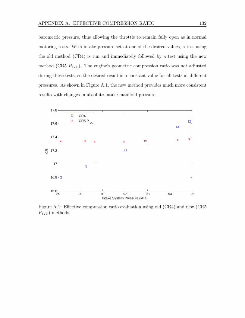
APPENDIX A. EFFECTIVE COMPRESSION RATIO 132
barometric pressure, thus allowing the throttle to remain fully open as in normal
motoring tests. With intake pressure set at one of the desired values, a test using
the old method (CR4) is run and immediately followed by a test using the new
method (CR5 P IVC). The engine’s geometric compression ratio was not adjusted
during these tests, so the desired result is a constant value for all tests at different
pressures. As shown in Figure A.1, the new method provides much more consistent
results with changes in absolute intake manifold pressure.
89 90 91 92 93 94 9516.6
16.8
17
17.2
17.4
17.6
17.8
Intake System Pressure (kPa)
CR
CR4CR5 P
IVC
Figure A.1: Effective compression ratio evaluation using old (CR4) and new (CR5P IVC) methods.
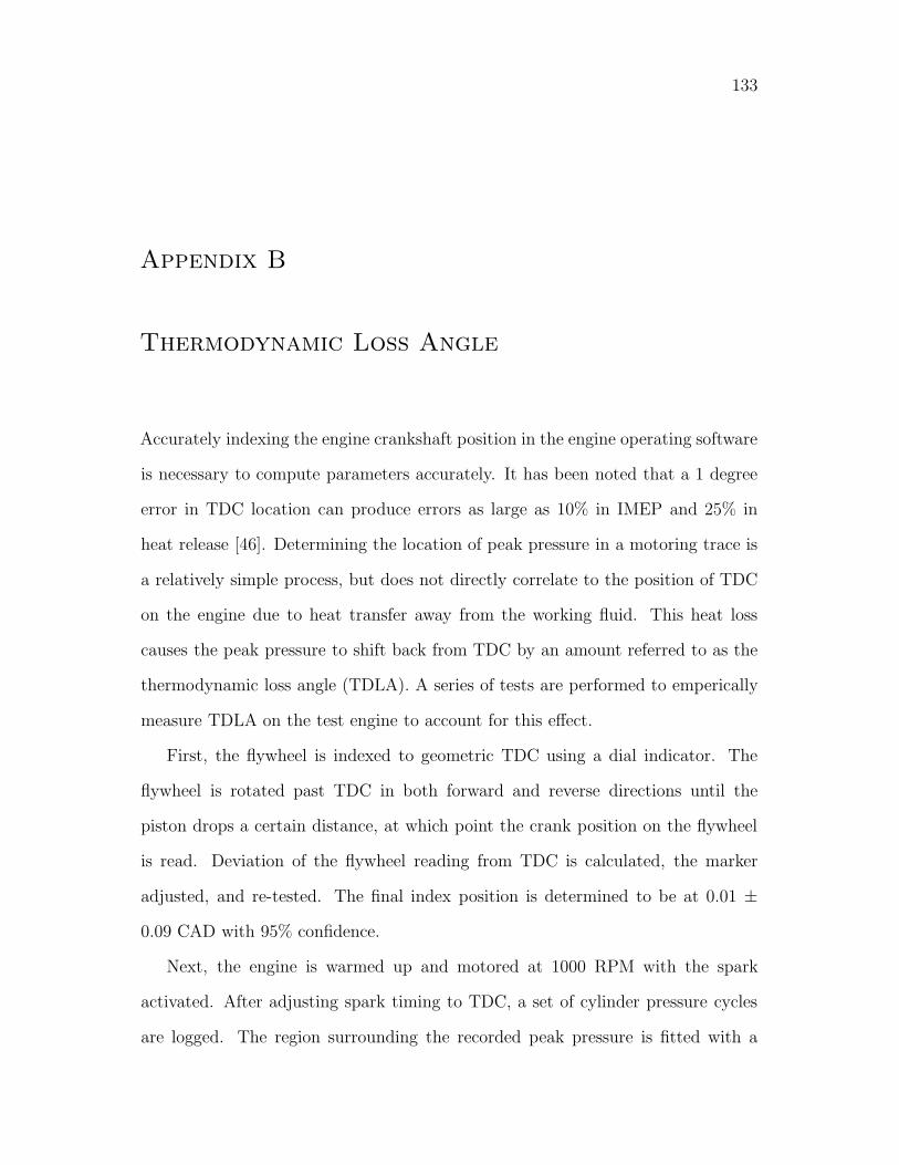
133
Appendix B
Thermodynamic Loss Angle
Accurately indexing the engine crankshaft position in the engine operating software
is necessary to compute parameters accurately. It has been noted that a 1 degree
error in TDC location can produce errors as large as 10% in IMEP and 25% in
heat release [46]. Determining the location of peak pressure in a motoring trace is
a relatively simple process, but does not directly correlate to the position of TDC
on the engine due to heat transfer away from the working fluid. This heat loss
causes the peak pressure to shift back from TDC by an amount referred to as the
thermodynamic loss angle (TDLA). A series of tests are performed to emperically
measure TDLA on the test engine to account for this effect.
First, the flywheel is indexed to geometric TDC using a dial indicator. The
flywheel is rotated past TDC in both forward and reverse directions until the
piston drops a certain distance, at which point the crank position on the flywheel
is read. Deviation of the flywheel reading from TDC is calculated, the marker
adjusted, and re-tested. The final index position is determined to be at 0.01 ±
0.09 CAD with 95% confidence.
Next, the engine is warmed up and motored at 1000 RPM with the spark
activated. After adjusting spark timing to TDC, a set of cylinder pressure cycles
are logged. The region surrounding the recorded peak pressure is fitted with a
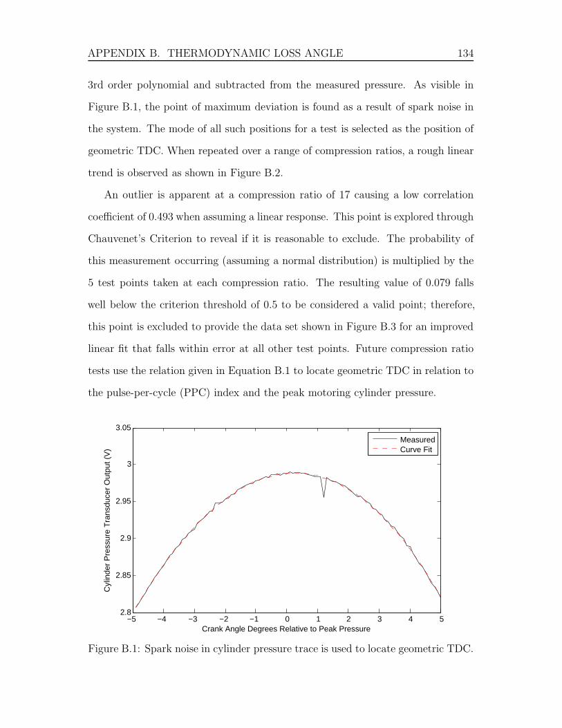
APPENDIX B. THERMODYNAMIC LOSS ANGLE 134
3rd order polynomial and subtracted from the measured pressure. As visible in
Figure B.1, the point of maximum deviation is found as a result of spark noise in
the system. The mode of all such positions for a test is selected as the position of
geometric TDC. When repeated over a range of compression ratios, a rough linear
trend is observed as shown in Figure B.2.
An outlier is apparent at a compression ratio of 17 causing a low correlation
coefficient of 0.493 when assuming a linear response. This point is explored through
Chauvenet’s Criterion to reveal if it is reasonable to exclude. The probability of
this measurement occurring (assuming a normal distribution) is multiplied by the
5 test points taken at each compression ratio. The resulting value of 0.079 falls
well below the criterion threshold of 0.5 to be considered a valid point; therefore,
this point is excluded to provide the data set shown in Figure B.3 for an improved
linear fit that falls within error at all other test points. Future compression ratio
tests use the relation given in Equation B.1 to locate geometric TDC in relation to
the pulse-per-cycle (PPC) index and the peak motoring cylinder pressure.
−5 −4 −3 −2 −1 0 1 2 3 4 52.8
2.85
2.9
2.95
3
3.05
Crank Angle Degrees Relative to Peak Pressure
Cyl
inde
r P
ress
ure
Tra
nsdu
cer
Out
put (
V)
MeasuredCurve Fit
Figure B.1: Spark noise in cylinder pressure trace is used to locate geometric TDC.
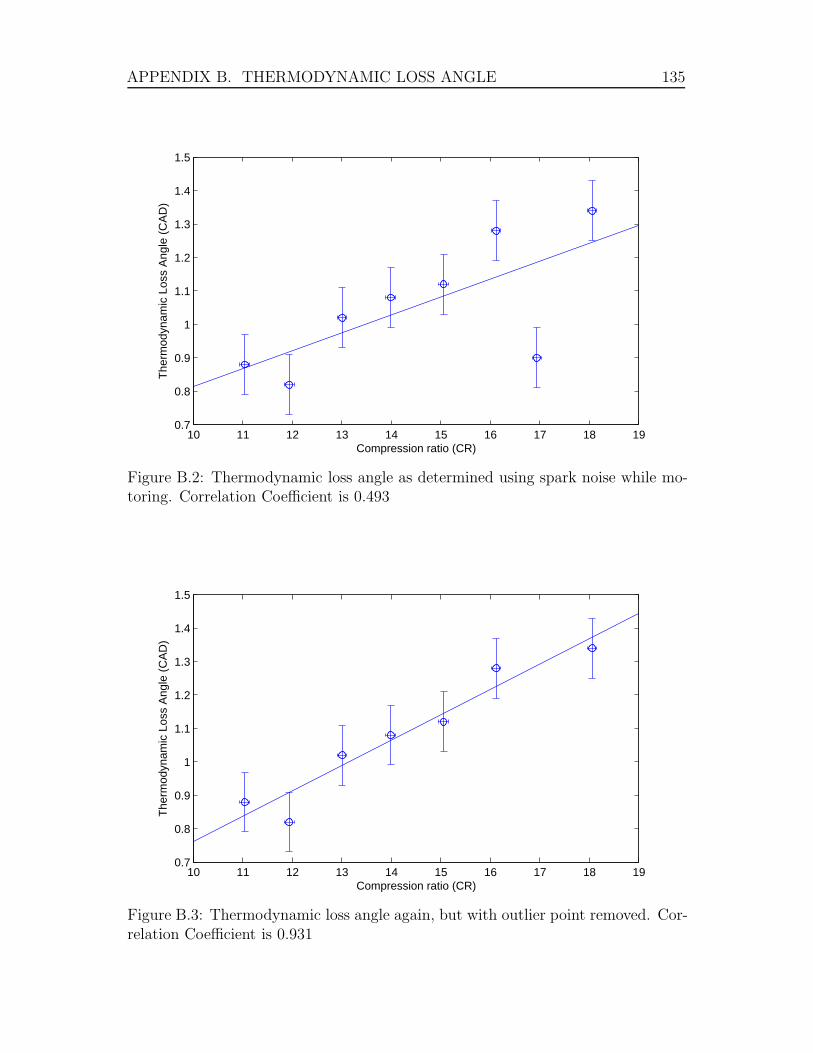
APPENDIX B. THERMODYNAMIC LOSS ANGLE 135
10 11 12 13 14 15 16 17 18 190.7
0.8
0.9
1
1.1
1.2
1.3
1.4
1.5
Compression ratio (CR)
The
rmod
ynam
ic L
oss
Ang
le (
CA
D)
Figure B.2: Thermodynamic loss angle as determined using spark noise while mo-toring. Correlation Coefficient is 0.493
10 11 12 13 14 15 16 17 18 190.7
0.8
0.9
1
1.1
1.2
1.3
1.4
1.5
Compression ratio (CR)
The
rmod
ynam
ic L
oss
Ang
le (
CA
D)
Figure B.3: Thermodynamic loss angle again, but with outlier point removed. Cor-relation Coefficient is 0.931

APPENDIX B. THERMODYNAMIC LOSS ANGLE 136
TDLA = 0.0756CR− 0.0059 CAD (B.1)

137
Appendix C
Intake Heat Loss Calculation
This appendix investigates the thermodynamic effects with the modified intake
manifold system that lead to a greater air temperature reduction than the original
large intake manifold setup. Consider temperature gradients in the heater manifold
pipe, polytropic expansion, the Joule-Thomson effect, heat transfer to the throttle
cooling lines, dilution cooling from the injected room-temperature CNG, intake
blow-back, and convection heat loss from the additional outside surfaces.
C.1 Heater Manifold Temperature Gradient
Air flow in the heater manifold pipe changes between SI and HCCI operation when
the throttle is located downstream. The intake system upstream of the throttle is
charged using building air and a pressure regulator. When the throttle is closed
to decrease the intake manifold pressure, the flow rate in the heater manifold is
reduced. By measuring the temperature profile immediately downstream of the air
heater, shown in Figure C.1, it becomes apparent that a shift in flow characteristics
exists between the two modes of operation. The visible temperature gradient in SI
suggests laminar flow with reduced mixing, while HCCI shows a more consistent
temperature across the diameter indicative of turbulent flow. Lower temperatures
at the top and bottom of the pipe in both scenarios suggest that these measurement
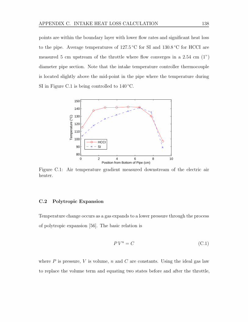
APPENDIX C. INTAKE HEAT LOSS CALCULATION 138
points are within the boundary layer with lower flow rates and significant heat loss
to the pipe. Average temperatures of 127.5 ◦C for SI and 130.8 ◦C for HCCI are
measured 5 cm upstream of the throttle where flow converges in a 2.54 cm (1”)
diameter pipe section. Note that the intake temperature controller thermocouple
is located slightly above the mid-point in the pipe where the temperature during
SI in Figure C.1 is being controlled to 140 ◦C.
0 2 4 6 8 1080
90
100
110
120
130
140
150
Position from Bottom of Pipe (cm)
Tem
pera
ture
(°C
)
HCCISI
Figure C.1: Air temperature gradient measured downstream of the electric airheater.
C.2 Polytropic Expansion
Temperature change occurs as a gas expands to a lower pressure through the process
of polytropic expansion [56]. The basic relation is
P V n = C (C.1)
where P is pressure, V is volume, n and C are constants. Using the ideal gas law
to replace the volume term and equating two states before and after the throttle,
APPENDIX C. INTAKE HEAT LOSS CALCULATION 139
the correlation between pressure and temperature is
T2
T1=
(
P1
P2
)n−1
n
(C.2)
The constant n depends on operating conditions and may vary between isothermal
(n = 1) and isentropic (n = k = 1.4 for air). Adiabatic conditions are assumed as
reasonable in the small vicinity around the throttle plate where the pressure drop
occurs.
Pressure measurements upstream and downstream of the throttle are presented
in Figures C.2 and C.3 at 700 RPM for SI and HCCI operation, respectively. For
choked flow during SI operation, air is moving past the throttle throughout the cycle
as indicated by the pressure difference. Considering the average of the two states,
the pressure upstream of the throttle is 125 kPa while being 70 kPa downstream.
HCCI operation shows that significant flow only occurs during and slightly after
the intake stroke, corresponding with the pressure drop during the intake stroke.
The pressure drop for polytropic expansion in this instance is considered only in
this region, being 114 kPa upstream and 106 kPa downstream of the throttle.
Evaluating Equation C.2 with these pressures and the average air temperatures
measured above in Section C.1 results in Table C.1 for several values of n. The
true value of n is difficult to predict and would require temperature measurements
in close vicinity of the throttle plate.
C.3 Joule-Thomson Effect
The Joule-Thomson effect is based on non-ideal properties of a gas as its pressure
is reduced [56]. Depending on the initial temperature of the gas in relation to
its inversion temperature, the gas temperature may either increase, decrease, or
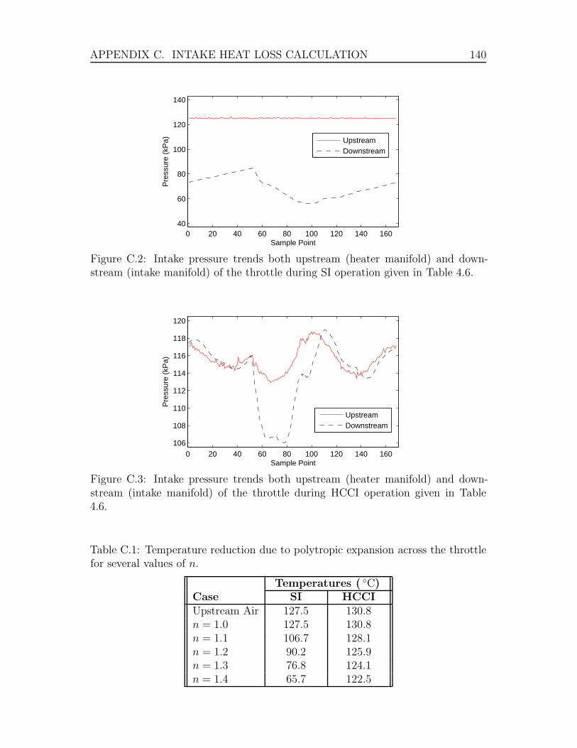
APPENDIX C. INTAKE HEAT LOSS CALCULATION 140
0 20 40 60 80 100 120 140 16040
60
80
100
120
140
Sample Point
Pre
ssur
e (k
Pa)
UpstreamDownstream
Figure C.2: Intake pressure trends both upstream (heater manifold) and down-stream (intake manifold) of the throttle during SI operation given in Table 4.6.
0 20 40 60 80 100 120 140 160106
108
110
112
114
116
118
120
Sample Point
Pre
ssur
e (k
Pa)
UpstreamDownstream
Figure C.3: Intake pressure trends both upstream (heater manifold) and down-stream (intake manifold) of the throttle during HCCI operation given in Table4.6.
Table C.1: Temperature reduction due to polytropic expansion across the throttlefor several values of n.
Temperatures ( ◦C)Case SI HCCIUpstream Air 127.5 130.8n = 1.0 127.5 130.8n = 1.1 106.7 128.1n = 1.2 90.2 125.9n = 1.3 76.8 124.1n = 1.4 65.7 122.5
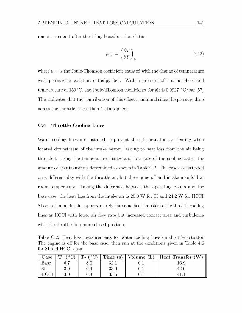
APPENDIX C. INTAKE HEAT LOSS CALCULATION 141
remain constant after throttling based on the relation
µJT =
(
∂T
∂P
)
h
(C.3)
where µJT is the Joule-Thomson coefficient equated with the change of temperature
with pressure at constant enthalpy [56]. With a pressure of 1 atmosphere and
temperature of 150 ◦C, the Joule-Thomson coefficienct for air is 0.0927 ◦C/bar [57].
This indicates that the contribution of this effect is minimal since the pressure drop
across the throttle is less than 1 atmosphere.
C.4 Throttle Cooling Lines
Water cooling lines are installed to prevent throttle actuator overheating when
located downstream of the intake heater, leading to heat loss from the air being
throttled. Using the temperature change and flow rate of the cooling water, the
amount of heat transfer is determined as shown in Table C.2. The base case is tested
on a different day with the throttle on, but the engine off and intake manifold at
room temperature. Taking the difference between the operating points and the
base case, the heat loss from the intake air is 25.0 W for SI and 24.2 W for HCCI.
SI operation maintains approximately the same heat transfer to the throttle cooling
lines as HCCI with lower air flow rate but increased contact area and turbulence
with the throttle in a more closed position.
Table C.2: Heat loss measurements for water cooling lines on throttle actuator.The engine is off for the base case, then run at the conditions given in Table 4.6for SI and HCCI data.
Case T1 ( ◦C) T2 ( ◦C) Time (s) Volume (L) Heat Transfer (W)Base 6.7 8.0 32.1 0.1 16.9SI 3.0 6.4 33.9 0.1 42.0HCCI 3.0 6.3 33.6 0.1 41.1
APPENDIX C. INTAKE HEAT LOSS CALCULATION 142
C.5 Convection
Heat loss from the outer surface of the throttle and additional aluminum fittings, as
visible in Figure 3.3, to the room air is evaluated by approximating these surfaces as
a cylinder with 3” diameter and 10” length [58]. Surface temperature of the throttle
and additional fittings are measured at four points and averaged to 79.5 ◦C and
84.3 ◦C during SI and HCCI operation, respectively, at the operating conditions in
Table 4.6. The higher temperature in HCCI is due to the higher mass flow rate and
air temperature for greater heat transfer from the hot manifold air to the throttle
and aluminum fittings.
The relations used to approximate convection heat loss to the room air are
summarized as follows:

APPENDIX C. INTAKE HEAT LOSS CALCULATION 143
GrD =g β(T s − T∞)L3
c
ν2(C.4a)
RaD = GrD Pr (C.4b)
Nu =
(
0.6 +0.387Ra
1/6D
[1 + (0.559/Pr)9/16]8/27
)2
(horizontal cylinder) (C.4c)
h =kNu
Lc(C.4d)
Qconv = hAconv (T s − T∞) (C.4e)
where
GrD = Grashof Number [−]
g = Gravitational Acceleration [m/s2]
β = V olumetric thermal expansion coefficient,
approximated as 1/T for ideal f luids [1/K]
T s = Surface Temperature [K]
T∞ = Room Temperature [K]
Lc = Characteristic Length [m]; Diameter for horizontal cylinder)
ν = Kinematic viscosity of the fluid [m2/s]
RaD = Rayleigh Number [−]
Pr = Prandtl Number [−]
Nu = Nusselt Number [−]
h = Average Convection Coefficient [W/m2 ◦C]
k = Thermal Conductivity [W/m ◦C]
Qconv = Convection Heat Transfer [W ]
Aconv = Area for Convection Heat Transfer [m2]
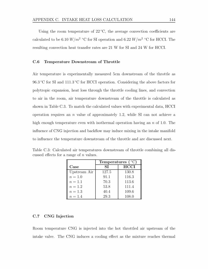
APPENDIX C. INTAKE HEAT LOSS CALCULATION 144
Using the room temperature of 22 ◦C, the average convection coefficients are
calculated to be 6.10 W/m2 ◦C for SI operation and 6.22 W/m2 ◦C for HCCI. The
resulting convection heat transfer rates are 21 W for SI and 24 W for HCCI.
C.6 Temperature Downstream of Throttle
Air temperature is experimentally measured 5cm downstream of the throttle as
96.3 ◦C for SI and 111.3 ◦C for HCCI operation. Considering the above factors for
polytropic expansion, heat loss through the throttle cooling lines, and convection
to air in the room, air temperature downstream of the throttle is calculated as
shown in Table C.3. To match the calculated values with experimental data, HCCI
operation requires an n value of approximately 1.2, while SI can not achieve a
high enough temperature even with isothermal operation having an n of 1.0. The
influence of CNG injection and backflow may induce mixing in the intake manifold
to influence the temperature downstream of the throttle and are discussed next.
Table C.3: Calculated air temperatures downstream of throttle combining all dis-cussed effects for a range of n values.
Temperatures ( ◦C)Case SI HCCIUpstream Air 127.5 130.8n = 1.0 91.1 116.3n = 1.1 70.3 113.6n = 1.2 53.8 111.4n = 1.3 40.4 109.6n = 1.4 29.3 108.0
C.7 CNG Injection
Room temperature CNG is injected into the hot throttled air upstream of the
intake valve. The CNG induces a cooling effect as the mixture reaches thermal

APPENDIX C. INTAKE HEAT LOSS CALCULATION 145
equilibrium. The final temperature is calculated using a thermodynamic balance
Tmix =(T air mair Cp air + T res mres Cp res)
(mairCp air + mres Cp CNG)(C.5)
where T is temperature, Cp is the constant pressure specific heat capacity, and
m is the mass flow rate for the indicated constituents. Temperature reduction in
Table C.4, compared with Table C.3 without CNG injection, is greater during SI
operation due to the larger mass fraction of CNG (stoichiometric as opposed to
lean in HCCI).
Table C.4: Calculated mixture temperatures after CNG injection for a range of nvalues.
Temperatures ( ◦C)Case SI HCCIUpstream Air 127.5 130.8n = 1.0 83.3 112.0n = 1.1 64.9 109.4n = 1.2 50.2 107.3n = 1.3 38.3 105.6n = 1.4 28.5 104.0
C.8 Backflow
Combustion products from the previous engine cycle can influence the intake mix-
ture temperature when the residual gas in the cylinder is at a higher pressure than
the intake manifold at IVO [1]. Hot exhaust gases may backflow into the intake
manifold during throttled operation in SI once the intake valve opens. With slow
engine speed and IVC occurring past BDC (see Table 3.3), there is potential for
gases to backflow into the intake manifold at the end of the intake stroke as well.
While the interaction occurring here is complex and depending on many variables,
a simplified approach is adopted to consider this effect.
First, cylinder volume at EVC is calculated using the slider-crank relation given
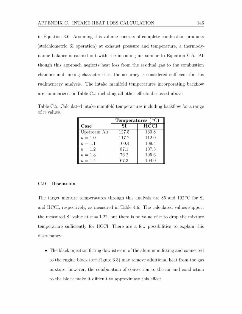
APPENDIX C. INTAKE HEAT LOSS CALCULATION 146
in Equation 3.6. Assuming this volume consists of complete combustion products
(stoichiometric SI operation) at exhaust pressure and temperature, a thermody-
namic balance is carried out with the incoming air similar to Equation C.5. Al-
though this approach neglects heat loss from the residual gas to the combustion
chamber and mixing characteristics, the accuracy is considered sufficient for this
rudimentary analysis. The intake manifold temperatures incorporating backflow
are summarized in Table C.5 including all other effects discussed above.
Table C.5: Calculated intake manifold temperatures including backflow for a rangeof n values.
Temperatures ( ◦C)Case SI HCCIUpstream Air 127.5 130.8n = 1.0 117.2 112.0n = 1.1 100.4 109.4n = 1.2 87.1 107.3n = 1.3 76.2 105.6n = 1.4 67.3 104.0
C.9 Discussion
The target mixture temperatures through this analysis are 85 and 102 ◦C for SI
and HCCI, respectively, as measured in Table 4.6. The calculated values support
the measured SI value at n = 1.22, but there is no value of n to drop the mixture
temperature sufficiently for HCCI. There are a few possibilities to explain this
discrepancy:� The black injection fitting downstream of the aluminum fitting and connected
to the engine block (see Figure 3.3) may remove additional heat from the gas
mixture; however, the combination of convection to the air and conduction
to the block make it difficult to approximate this effect.

APPENDIX C. INTAKE HEAT LOSS CALCULATION 147� Convection heat loss from all surfaces may be higher than calculated. The
exposed surface area is approximated by a cylinder, which is not the actual
surface area. Further, convection from the non-cylindrical geometry may
deviate from the empirical relations for natural convection from a horizontal
cylinder.� Air movement in the room from exhaust fans may induce some forced convec-
tion to increase heat transfer away from the throttle and additional fittings.
With the small difference between the measured and calculated mixture temper-
atures, this analysis validates the need for a higher intake air set point of 140 ◦C
with the throttle position downstream of the intake heater for the small intake
manifold.
148
Appendix D
Sensor Calibrations
All sensors used during engine testing are calibrated on a regular basis. Following
are detailed descriptions of the equipment and procedures used along with the
resulting calibrations. Note that in some figures the error bars are small enough
to fall inside the data point markers.
Error is presented in the calibration plots using 95% confidence intervals. A sin-
gle error value is selected for each instrument by comparing the average of the 95%
confidence interval with two standard deviations of the residual. The two values
generally fall very close to one another with any significant differences discussed
for the specific case.
D.1 Air Mass Flow
The TSI 42350101 hot wire anemometer is calibrated using a 5 cubic foot Bell
Prover made available in the Chemical Engineering Department at the University
of Alberta. Air is supplied through the same regulator and 0.5” ID rubber hose as
on the engine. Air flow first passes through the TSI meter and then into the Bell
Prover. All connections are leak tested prior to calibrating.
Using the same DAQ computer and hardware as on the engine, a series of tests
are run. First, the regulator is set to the desired rate as defined by a given voltage
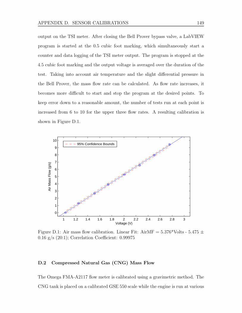
APPENDIX D. SENSOR CALIBRATIONS 149
output on the TSI meter. After closing the Bell Prover bypass valve, a LabVIEW
program is started at the 0.5 cubic foot marking, which simultaneously start a
counter and data logging of the TSI meter output. The program is stopped at the
4.5 cubic foot marking and the output voltage is averaged over the duration of the
test. Taking into account air temperature and the slight differential pressure in
the Bell Prover, the mass flow rate can be calculated. As flow rate increases, it
becomes more difficult to start and stop the program at the desired points. To
keep error down to a reasonable amount, the number of tests run at each point is
increased from 6 to 10 for the upper three flow rates. A resulting calibration is
shown in Figure D.1.
1 1.2 1.4 1.6 1.8 2 2.2 2.4 2.6 2.8 3
0
1
2
3
4
5
6
7
8
9
10
Voltage (V)
Air
Mas
s F
low
(g/
s)
95% Confidence Bounds
Figure D.1: Air mass flow calibration. Linear Fit: AirMF = 5.376*Volts - 5.475 ±0.16 g/s (20:1); Correlation Coefficient: 0.99975
D.2 Compressed Natural Gas (CNG) Mass Flow
The Omega FMA-A2117 flow meter is calibrated using a gravimetric method. The
CNG tank is placed on a calibrated GSE 550 scale while the engine is run at various
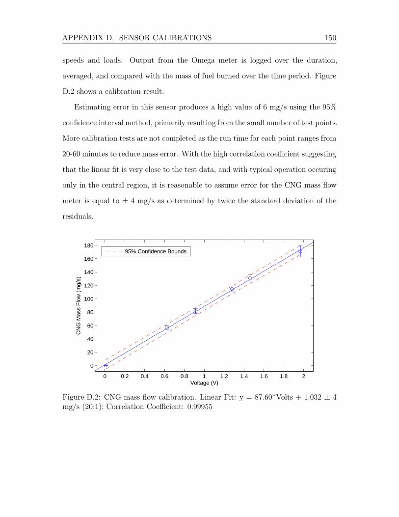
APPENDIX D. SENSOR CALIBRATIONS 150
speeds and loads. Output from the Omega meter is logged over the duration,
averaged, and compared with the mass of fuel burned over the time period. Figure
D.2 shows a calibration result.
Estimating error in this sensor produces a high value of 6 mg/s using the 95%
confidence interval method, primarily resulting from the small number of test points.
More calibration tests are not completed as the run time for each point ranges from
20-60 minutes to reduce mass error. With the high correlation coefficient suggesting
that the linear fit is very close to the test data, and with typical operation occuring
only in the central region, it is reasonable to assume error for the CNG mass flow
meter is equal to ± 4 mg/s as determined by twice the standard deviation of the
residuals.
0 0.2 0.4 0.6 0.8 1 1.2 1.4 1.6 1.8 2
0
20
40
60
80
100
120
140
160
180
Voltage (V)
CN
G M
ass
Flo
w (
mg/
s)
95% Confidence Bounds
Figure D.2: CNG mass flow calibration. Linear Fit: y = 87.60*Volts + 1.032 ± 4mg/s (20:1); Correlation Coefficient: 0.99955
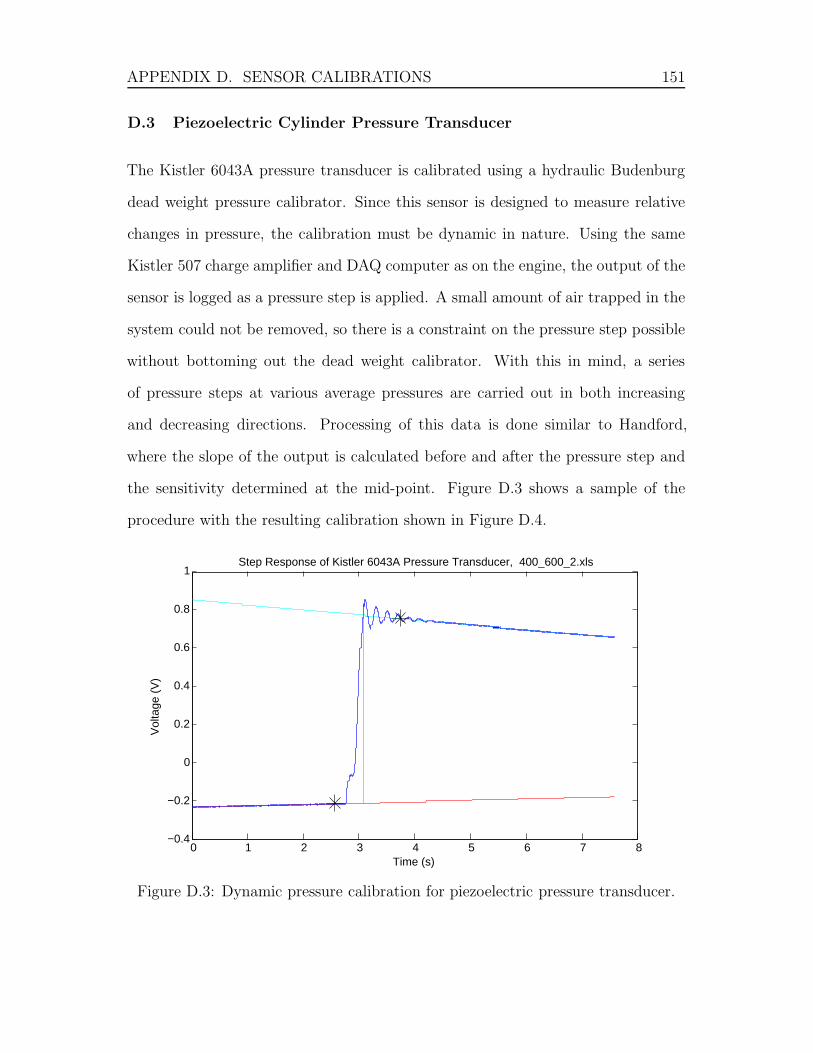
APPENDIX D. SENSOR CALIBRATIONS 151
D.3 Piezoelectric Cylinder Pressure Transducer
The Kistler 6043A pressure transducer is calibrated using a hydraulic Budenburg
dead weight pressure calibrator. Since this sensor is designed to measure relative
changes in pressure, the calibration must be dynamic in nature. Using the same
Kistler 507 charge amplifier and DAQ computer as on the engine, the output of the
sensor is logged as a pressure step is applied. A small amount of air trapped in the
system could not be removed, so there is a constraint on the pressure step possible
without bottoming out the dead weight calibrator. With this in mind, a series
of pressure steps at various average pressures are carried out in both increasing
and decreasing directions. Processing of this data is done similar to Handford,
where the slope of the output is calculated before and after the pressure step and
the sensitivity determined at the mid-point. Figure D.3 shows a sample of the
procedure with the resulting calibration shown in Figure D.4.
0 1 2 3 4 5 6 7 8−0.4
−0.2
0
0.2
0.4
0.6
0.8
1Step Response of Kistler 6043A Pressure Transducer, 400_600_2.xls
Time (s)
Vol
tage
(V
)
Figure D.3: Dynamic pressure calibration for piezoelectric pressure transducer.
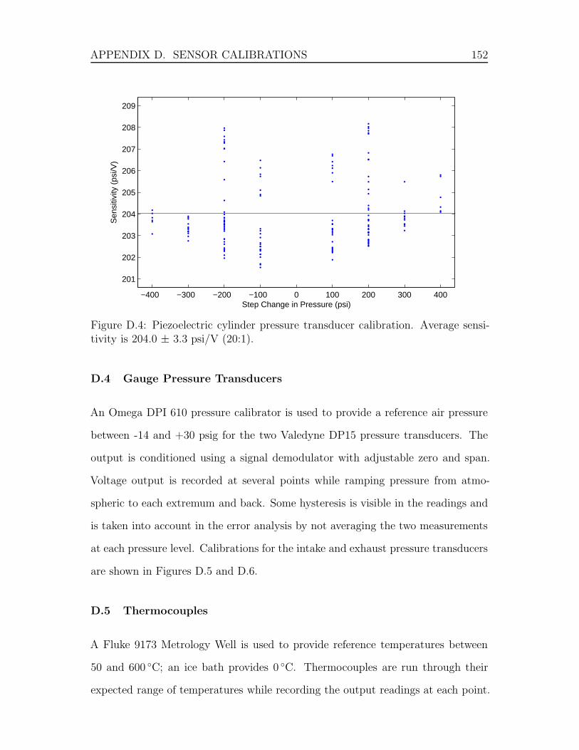
APPENDIX D. SENSOR CALIBRATIONS 152
−400 −300 −200 −100 0 100 200 300 400
201
202
203
204
205
206
207
208
209
Step Change in Pressure (psi)
Sen
sitiv
ity (
psi/V
)
Figure D.4: Piezoelectric cylinder pressure transducer calibration. Average sensi-tivity is 204.0 ± 3.3 psi/V (20:1).
D.4 Gauge Pressure Transducers
An Omega DPI 610 pressure calibrator is used to provide a reference air pressure
between -14 and +30 psig for the two Valedyne DP15 pressure transducers. The
output is conditioned using a signal demodulator with adjustable zero and span.
Voltage output is recorded at several points while ramping pressure from atmo-
spheric to each extremum and back. Some hysteresis is visible in the readings and
is taken into account in the error analysis by not averaging the two measurements
at each pressure level. Calibrations for the intake and exhaust pressure transducers
are shown in Figures D.5 and D.6.
D.5 Thermocouples
A Fluke 9173 Metrology Well is used to provide reference temperatures between
50 and 600 ◦C; an ice bath provides 0 ◦C. Thermocouples are run through their
expected range of temperatures while recording the output readings at each point.
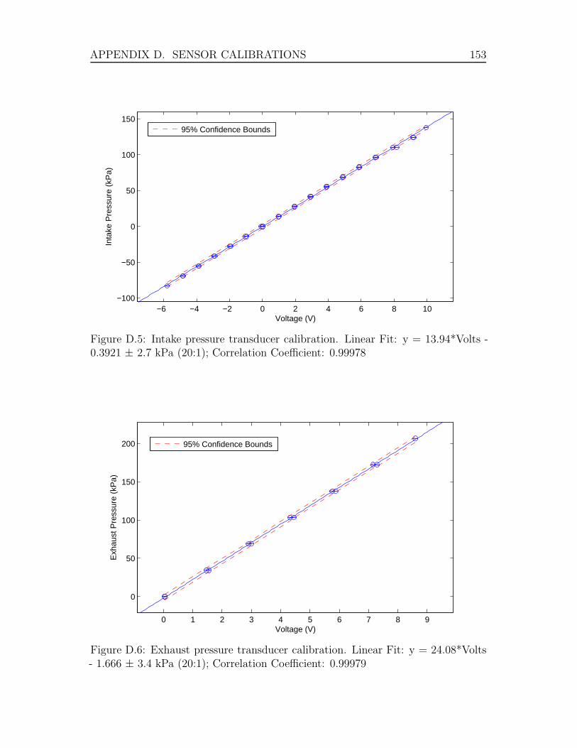
APPENDIX D. SENSOR CALIBRATIONS 153
−6 −4 −2 0 2 4 6 8 10−100
−50
0
50
100
150
Voltage (V)
Inta
ke P
ress
ure
(kP
a)
95% Confidence Bounds
Figure D.5: Intake pressure transducer calibration. Linear Fit: y = 13.94*Volts -0.3921 ± 2.7 kPa (20:1); Correlation Coefficient: 0.99978
0 1 2 3 4 5 6 7 8 9
0
50
100
150
200
Voltage (V)
Exh
aust
Pre
ssur
e (k
Pa)
95% Confidence Bounds
Figure D.6: Exhaust pressure transducer calibration. Linear Fit: y = 24.08*Volts- 1.666 ± 3.4 kPa (20:1); Correlation Coefficient: 0.99979
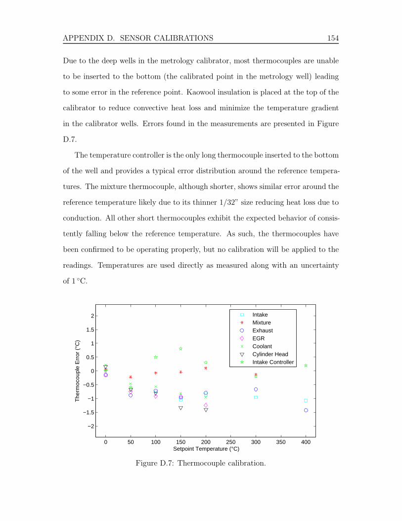
APPENDIX D. SENSOR CALIBRATIONS 154
Due to the deep wells in the metrology calibrator, most thermocouples are unable
to be inserted to the bottom (the calibrated point in the metrology well) leading
to some error in the reference point. Kaowool insulation is placed at the top of the
calibrator to reduce convective heat loss and minimize the temperature gradient
in the calibrator wells. Errors found in the measurements are presented in Figure
D.7.
The temperature controller is the only long thermocouple inserted to the bottom
of the well and provides a typical error distribution around the reference tempera-
tures. The mixture thermocouple, although shorter, shows similar error around the
reference temperature likely due to its thinner 1/32” size reducing heat loss due to
conduction. All other short thermocouples exhibit the expected behavior of consis-
tently falling below the reference temperature. As such, the thermocouples have
been confirmed to be operating properly, but no calibration will be applied to the
readings. Temperatures are used directly as measured along with an uncertainty
of 1 ◦C.
0 50 100 150 200 250 300 350 400
−2
−1.5
−1
−0.5
0
0.5
1
1.5
2
Setpoint Temperature (°C)
The
rmoc
oupl
e E
rror
(°C
)
IntakeMixtureExhaustEGRCoolantCylinder HeadIntake Controller
Figure D.7: Thermocouple calibration.
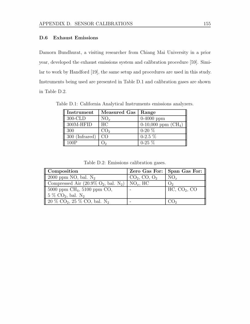
APPENDIX D. SENSOR CALIBRATIONS 155
D.6 Exhaust Emissions
Damorn Bundhurat, a visiting researcher from Chiang Mai University in a prior
year, developed the exhaust emissions system and calibration procedure [59]. Simi-
lar to work by Handford [19], the same setup and procedures are used in this study.
Instruments being used are presented in Table D.1 and calibration gases are shown
in Table D.2.
Table D.1: California Analytical Instruments emissions analyzers.
Instrument Measured Gas Range300-CLD NOx 0-4000 ppm300M-HFID HC 0-10,000 ppm (CH4)300 CO2 0-20 %300 (Infrared) CO 0-2.5 %100P O2 0-25 %
Table D.2: Emissions calibration gases.
Composition Zero Gas For: Span Gas For:2000 ppm NO, bal. N2 CO2, CO, O2 NOx
Compressed Air (20.9% O2, bal. N2) NOx, HC O2
5000 ppm CH4, 5100 ppm CO, - HC, CO2, CO5 % CO2, bal. N2
20 % CO2, 25 % CO, bal. N2 - CO2
156
Appendix E
Uncertainty Analysis
The uncertainty associated with measured and calculated parameters are evaluated
in this appendix.
E.1 Average Intake Pressure
Error in this cyclical measurement is calculated by considering both the accuracy of
the calibrated intake pressure sensor and the variability in the measurement. Dur-
ing a motoring test, the engine is held at steady-state conditions while 100 cycles
are recorded. Observing the variability in the recorded values gives an indication
of uncertainty in to measurement.
For the instance of intake pressure, a standard deviation of 0.023 kPa is observed.
Since greater than 30 samples are considered, the uncertainty due to variability is
taken as twice the standard deviation. Combining this value with the calibration
uncertainty is accomplished using a root sum of the squares (RSS) approach [60]
using
δR =
√
√
√
√
Num∑
i=1
δX2i (E.1)
where δR is the uncertainty in the result, δXi is the uncertainty of each component
being considered, and Num is the number of uncertainty components. The total
APPENDIX E. UNCERTAINTY ANALYSIS 157
uncertainty for intake pressure is thus found to be 2.7 kPa. As expected, the low
variability of the measurement does not have a significant influence on the total
uncertainty as dictated by the calibration uncertainty.
E.2 P IVC
Pressure at IVC is determined by averaging 5% of the intake pressure measure-
ments immediately prior to IVC as discussed in Section 3.1.2.1. Using the same
approach as described above for intake pressure, the standard deviation in P IVC
while motoring is found to be 0.71 kPa. Since only 8 samples are used in this mea-
surement, a Student’s t-test is applied to determine uncertainty due to variability.
Combining the result with calibrational uncertainty using a RSS results in a total
uncertainty in P IVC of 2.8 kPa with 95% confidence.
One aspect of error that can not be easily evaluated is the correlation between
average intake pressure or P IVC and air mass flow during fast changes in throttle
position. Without the proper equipment to measure air mass induction on each
engine cycle, the effect can only be speculated upon.
With a large change in throttle position, the air pressure on both sides of the
throttle experience conditions not representative of steady-state operation. The
manifold pressure is likely to drift up or down throughout the engine cycle as the
intake system tends toward stability. Conditions present while the intake valve
is open may not correlate with the average throughout the cycle; however, P IVC
should provide a more representative value of the engine conditions due to its
shorter duration and specific location relative to IVC. This capability allows for a
more accurate prediction of cycle specific equivalence ratio during mode-switching
when using P IVC as opposed to average intake pressure.
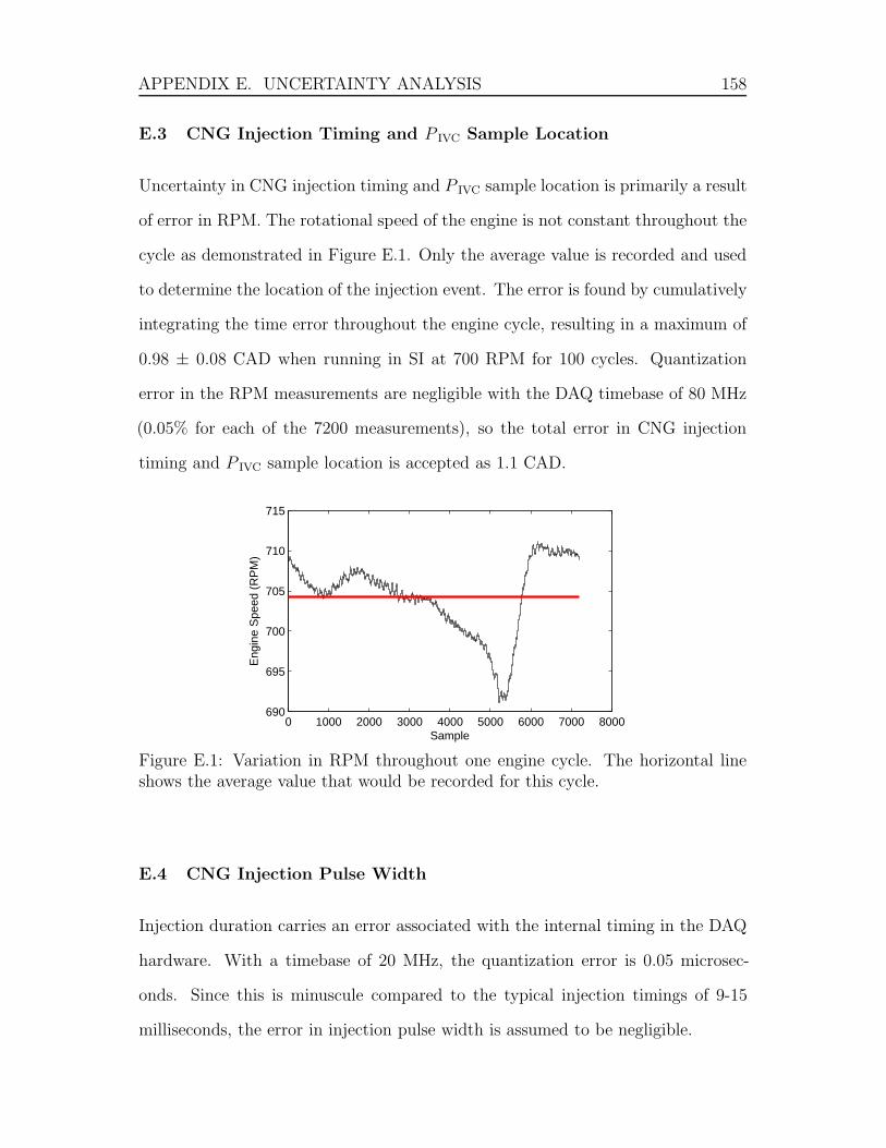
APPENDIX E. UNCERTAINTY ANALYSIS 158
E.3 CNG Injection Timing and P IVC Sample Location
Uncertainty in CNG injection timing and P IVC sample location is primarily a result
of error in RPM. The rotational speed of the engine is not constant throughout the
cycle as demonstrated in Figure E.1. Only the average value is recorded and used
to determine the location of the injection event. The error is found by cumulatively
integrating the time error throughout the engine cycle, resulting in a maximum of
0.98 ± 0.08 CAD when running in SI at 700 RPM for 100 cycles. Quantization
error in the RPM measurements are negligible with the DAQ timebase of 80 MHz
(0.05% for each of the 7200 measurements), so the total error in CNG injection
timing and P IVC sample location is accepted as 1.1 CAD.
0 1000 2000 3000 4000 5000 6000 7000 8000690
695
700
705
710
715
Sample
Eng
ine
Spe
ed (
RP
M)
Figure E.1: Variation in RPM throughout one engine cycle. The horizontal lineshows the average value that would be recorded for this cycle.
E.4 CNG Injection Pulse Width
Injection duration carries an error associated with the internal timing in the DAQ
hardware. With a timebase of 20 MHz, the quantization error is 0.05 microsec-
onds. Since this is minuscule compared to the typical injection timings of 9-15
milliseconds, the error in injection pulse width is assumed to be negligible.
APPENDIX E. UNCERTAINTY ANALYSIS 159
E.5 IMEP
Indicated mean effective pressure is calculated using the recorded in-cylinder pres-
sure trace. The piezoelectric pressure transducer that samples cylinder pressure
carries a quoted accuracy of 8.8% for each individual measurement. Since IMEP
is evaluated as the integral of pressure over volume throughout one engine cycle,
the total error is reduced by dividing by the square root of the number of samples
per cycle, which in this study is 7200. The resulting calculation error for IMEP is
0.1%.
Variability from cycle to cycle generally contributes a larger error than the
calculated error, but this will depend on the stability of the operating point. Since
the focus of this study is observing cycles individually, measurement variability
must be evaluated independently. Data obtained while motoring is used as this
constitutes very stable engine operation to observe measurement uncertainty as
opposed to operational variability. A standard deviation of 0.03 bar for IMEP is
found among the 100 cycles. With the calculation error being significantly lower
than the variability for the approximate IMEP range of 3-5 bar experienced in this
study, the total error in IMEP is taken as 0.06 bar with 95% confidence.
E.6 CA50
The location of 50% fuel mass burned is determined from the rate of heat release,
which in turn is calculated using the cylinder pressure trace. Handford investigated
the error in this calculation by applying a Monte Carlo algorithm that varied the
heat transfer coefficienct by ± 50% resulting in an error of 0.83 CAD in CA50
with 95% confidence [19]. For this study, the same procedures is implemented
during HCCI operation, but the original Woschni heat transfer coefficients are im-
plemented during SI operation. Table E.1 lists the results of applying a Monte
APPENDIX E. UNCERTAINTY ANALYSIS 160
Carlo algorithm to the different combinations of heat transfer coefficients and com-
bustion types. Note that the uncertainty of evaluating CA50 for HCCI combustion
with HCCI heat transfer coefficients is very close to the value obtained by Handford.
Table E.1: Monte Carlo algorithm applied to CA50 calculation using SI and HCCIheat transfer coefficients for SI and HCCI combustion cycles. Values are given in◦aTDC.
Heat Transfer Coefficients SI HCCICombustion Type SI HCCI SI HCCIAverage CA50 48.29 38.54 10.14 4.8695% Uncertainty in CA50 3.05 1.91 0.69 0.89
E.7 ROPR
The maximum rate of pressure rise is determined from the cylinder pressure trace
after applying a low-pass butterworth filter with a normalized cutoff frequency of
0.10. The filter reduces noise in the measurements to provide a more appropriate
value for maximum slope, but complicates a numerical evaluation of this error.
Variability of this parameter with the system during stable operation should provide
a representative value. While motoring, the standard deviation in ROPR is found
to be 0.016 bar/CAD over 100 cycles. Using this to support the assumption that the
low-pass filter sufficiently dampens out cylinder pressure measurement fluctuations,
the error in ROPR is taken as 0.03 bar/CAD with 95% confidence.
E.8 Equivalence Ratio
Equivalence ratio is calculated based on the mass of CNG and air inducted during
each engine cycle as presented in Equation 3.1. As discussed in Section 3.1.4, these
two quantities are determined from correlations of CNG mass flow rate with CNG
injection pulse width, and air mass flow rate with P IVC.
APPENDIX E. UNCERTAINTY ANALYSIS 161
E.8.1 CNG Mass Per Cycle
Figure 3.9 shows the relationship between CNG mass flow rate and injection pulse
width. Considering two standard deviations of the residuals, the error in the CNG
mass per cycle is 0.15 milligrams with 95% confidence. The strong linear trend in
the data leads to this low error in the best fit line; however, the uncertainty in each
of the measurements should be carried through for future calculations. Starting
with the CNG mass flow error of 4 mg/s, the error in CNG mass per injection is
converted to 0.68 mg/cycle with 95% confidence. Combining this with the residual
error through a RSS, the total error becomes 0.7 mg/cycle with 95% confidence.
E.8.2 Air Mass Per Cycle
Initially, the volumetric efficiency of the engine at various P IVC values is determined
as discussed in Section 3.1.4. The error in the resulting values is determined through
a means of perturbing the inputs individually and taking the RSS of all contributing
factors [60]. When using the absolute errors associated with the measurements as
calculated in Appendix D, the absolute error in volumetric efficiency becomes 0.07
with 95% confidence. This error is large relative to the observed trend in volumetric
efficiency values. The uncertainty is reduced significantly when considering only
the variability in the test runs and not the bias error associated with calibration.
This is reasonable for the characterization of volumetric efficiency with P IVC as
these values are only intended for use on this engine with the current measurement
system; however, the benefit of this approach is limited to differentiatng between
volumetric efficiencies during this characterization. The total uncertainty of 0.07
must be considered in successive calculations using volumetric efficiency based on
this data.
Next, the air mass is calculated for individual cycles during mode-switching.
Volumetric efficiency is determined from the measured P IVC based on Figure 3.12
APPENDIX E. UNCERTAINTY ANALYSIS 162
before solving for air mass flow rate through an iterative approach. Engine speed
is used to determine the mass of air induced on a single cycle as opposed to an
average air mass flow rate. Error throughout these calculations is again determined
by perturbing the inputs by their associated uncertainties, resulting in an overall
uncertainty of 12% in the calculated equivalence ratio with 95% confidence.
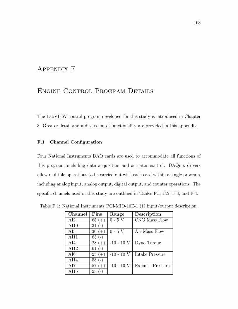
163
Appendix F
Engine Control Program Details
The LabVIEW control program developed for this study is introduced in Chapter
3. Greater detail and a discussion of functionality are provided in this appendix.
F.1 Channel Configuration
Four National Instruments DAQ cards are used to accommodate all functions of
this program, including data acquisition and actuator control. DAQmx drivers
allow multiple operations to be carried out with each card within a single program,
including analog input, analog output, digital output, and counter operations. The
specific channels used in this study are outlined in Tables F.1, F.2, F.3, and F.4.
Table F.1: National Instruments PCI-MIO-16E-1 (1) input/output description.
Channel Pins Range DescriptionAI2 65 (+) 0 - 5 V CNG Mass FlowAI10 31 (-)AI3 30 (+) 0 - 5 V Air Mass FlowAI11 63 (-)AI4 28 (+) -10 - 10 V Dyno TorqueAI12 61 (-)AI6 25 (+) -10 - 10 V Intake PressureAI14 58 (-)AI7 57 (+) -10 - 10 V Exhaust PressureAI15 23 (-)

APPENDIX F. ENGINE CONTROL PROGRAM DETAILS 164
Table F.2: National Instruments PCI-MIO-16E-1 (2) input/output description.
Channel Pins Range DescriptionAI0 68 (+) - CJCAI8 34 (-)AI2 65 (+) 0 - 200 ◦C Intake Mixture ThermocoupleAI10 31 (-) (1/32”, Type J)AI3 30 (+) 0 - 400 ◦C Intake Air ThermocoupleAI11 63 (-) (1/16”, Type J)AI4 28 (+) 0 - 200 ◦C EGR ThermocoupleAI12 61 (-) (1/16”, Type J)AI5 60 (+) 0 - 200 ◦C Coolant ThermocoupleAI13 26 (-) (1/16”, Type T)AI6 25 (+) 0 - 600 ◦C Exhaust ThermocoupleAI14 58 (-) (1/16”, Type J)AI7 57 (+) 0 - 200 ◦C Cylinder Head ThermocoupleAI15 23 (-) (1/8”, Type T)CTR0 3 (+) - Cam SignalDGND 36 (GND)CTR0 Out 2 (+) 0 - 5 V CNG Injector SignalDGND 36 (GND)
Table F.3: National Instruments PCI-MIO-16E-4 input/output description.
Channel Pins Range DescriptionAI2 65 (+) 0 - 10 V NOx EmissionsAI10 31 (-)AI3 30 (+) 0 - 10 V HC EmissionsAI11 63 (-)AI4 28 (+) 0 - 10 V TPS FeedbackAI12 61 (-)AI5 60 (+) 0 - 10 V CO2 EmissionsAI13 26 (-)AI6 25 (+) 0 - 10 V CO EmissionsAI14 58 (-)AI7 57 (+) 0 - 10 V O2 EmissionsAI15 23 (-)AO0 22 (+) 0 - 5 V Throttle ControlAOGND 55 (GND)DIO0 52 (+) 0 - 5 V Spark SolenoidDGND 18 (GND)
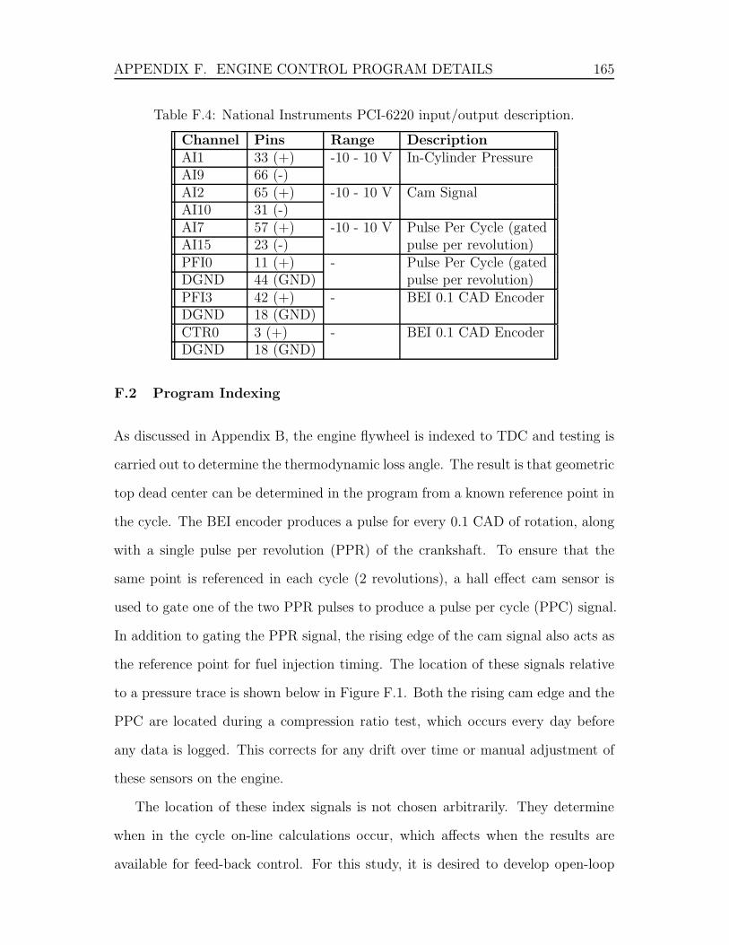
APPENDIX F. ENGINE CONTROL PROGRAM DETAILS 165
Table F.4: National Instruments PCI-6220 input/output description.
Channel Pins Range DescriptionAI1 33 (+) -10 - 10 V In-Cylinder PressureAI9 66 (-)AI2 65 (+) -10 - 10 V Cam SignalAI10 31 (-)AI7 57 (+) -10 - 10 V Pulse Per Cycle (gatedAI15 23 (-) pulse per revolution)PFI0 11 (+) - Pulse Per Cycle (gatedDGND 44 (GND) pulse per revolution)PFI3 42 (+) - BEI 0.1 CAD EncoderDGND 18 (GND)CTR0 3 (+) - BEI 0.1 CAD EncoderDGND 18 (GND)
F.2 Program Indexing
As discussed in Appendix B, the engine flywheel is indexed to TDC and testing is
carried out to determine the thermodynamic loss angle. The result is that geometric
top dead center can be determined in the program from a known reference point in
the cycle. The BEI encoder produces a pulse for every 0.1 CAD of rotation, along
with a single pulse per revolution (PPR) of the crankshaft. To ensure that the
same point is referenced in each cycle (2 revolutions), a hall effect cam sensor is
used to gate one of the two PPR pulses to produce a pulse per cycle (PPC) signal.
In addition to gating the PPR signal, the rising edge of the cam signal also acts as
the reference point for fuel injection timing. The location of these signals relative
to a pressure trace is shown below in Figure F.1. Both the rising cam edge and the
PPC are located during a compression ratio test, which occurs every day before
any data is logged. This corrects for any drift over time or manual adjustment of
these sensors on the engine.
The location of these index signals is not chosen arbitrarily. They determine
when in the cycle on-line calculations occur, which affects when the results are
available for feed-back control. For this study, it is desired to develop open-loop

APPENDIX F. ENGINE CONTROL PROGRAM DETAILS 166
0 100 200 300 400 500 600 700
0
20
40
Cyl
inde
rP
ress
ure
(bar
)
0
2
4
PP
R S
igna
l (V
)
0
2
4
Cam
Sig
nal (
V)
0 100 200 300 400 500 600 7000
2
4
PP
C S
igna
l (V
)
Crank Angle Degrees
Figure F.1: Index signals used for fuel injection timing and to locate TDC duringa compression ratio test.

APPENDIX F. ENGINE CONTROL PROGRAM DETAILS 167
control sequences to control mode-switching, so it is important to have a system
capable of producing repeatable actuator response. PI feed-back is implemented
following the mode-switch to maintain stable operation in HCCI because of the
relatively low intake temperatures being used. Since variable fuel injection timing is
used during this study, it is also important to understand how the system responds
to changes throughout the engine cycle.
The cam signal must be set in relation to the PPR signal, as it must gate one
of the two PPR pulses to create the PPC signal using discrete logic TTL circuitry.
After setting the desired PPR pulse timing, the cam signal is adjusted so the falling
edge occurs slightly ahead of the PPR signal. This provides the greatest time before
the rising edge occurs from which the fuel injection timing is referenced.
The PPC signal determines the point at which data transfer occurs for all DAQ
signals. By setting this to occur just after EVO, all useful information from the
previous cycle is recorded and available for calculation. The compression and ex-
pansion phases of the cylinder pressure trace are available for combustion analysis,
and the intake measurements correlate with the recorded pressure trace to ensure
data synchronization. The exhaust stroke provides sufficient time for the program
to run all on-line computations for feedback control of the next cycle.
There is a limitation to achieve next cycle fuel control such that fuel injection
must occur slightly before or during the intake stroke. If injection timing is set after
IVC, then the fuel injection event will only affect the following cycle’s combustion
as it will remain in the intake manifold until that time. Injection during the
calculation time is not possible as the system “skips” every second cycle due to
the extended time delay associated with the fuel signal. An external fuel controller
may remedy this situation, but would not receive the new fuel parameters until the
combustion calculations are completed, thus preventing next cycle fuel control in
this region.
APPENDIX F. ENGINE CONTROL PROGRAM DETAILS 168
This concern is handled by restricting injection timing to the stable region,
thus excluding the injection from 220◦ bIVO to IVO (during the exhaust stroke).
Injection during the later portion of the intake stroke is avoided to ensure all CNG is
induced on a single cycle, so only injection at IVO is used for next cycle fuel control.
As a result, advancing the injection timing from anywhere between IVC and 220◦
bIVO (which fuels the following cycle) to IVO (which fuels the current cycle) must
be completed while commanding one cycle of no fuel delivery to avoid double-
fueling the next engine cycle. Conversely, adjusting injection timing in the opposite
direction from IVO to anywhere between IVC and 220◦ bIVO inherently provides
one cycle without fuel, causing a mis-fire. This is relegated by avoiding this type
of injection timing adjustment during a mode-switch as would be desirable during
HCCI-SI. Instead, the injection timing is advanced to 220◦ bIVO and the engine
allowed to stabilize before initiating the mode-switch. Further control programming
could allow for a double-injection when this type of adjustment is made, but the
added complexity was deemed unnecessary for this study.
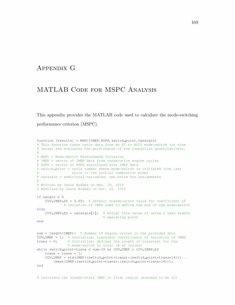
169
Appendix G
MATLAB Code for MSPC Analysis
This appendix provides the MATLAB code used to calculate the mode-switching
performance criterion (MSPC).
function [results] = MSPC(IMEP,ROPR,switch point,varargin)% This function takes cycle data from an SI to HCCI mode −switch (or vice% versa) and evaluates the performance of the transition qua ntitatively.%% MSPC = Mode−Switch Performance Criterion% IMEP = vector of IMEP data from consecutive engine cycles% ROPR = vector of ROPR associated with IMEP data% switch point = cycle number where mode −switch is initiated (the last% cycle in the initial combustion mode)% varargin = additional variables; see below for assignment s%% Written by Jason Boddez on Mar. 19, 2010% Modified by Jason Boddez on Oct. 22, 2010
if nargin < 4COVIMEP SS = 0.05; % Default steady −state value for coefficient of
% variation of IMEP used to define the end of the mode −switchelse
COVIMEP SS = varargin {1}; % Adjust this value if using a less stable% operating point
end
num = length(IMEP); % Number of engine cycles in the provided dataCOVIMEP = 1; % Initialize; transient coefficienct of variation of IMEPtrans = 0; % Initialize; defines the length of transient for the
% mode−switch to occur (# of cycles)while switch point+trans < num−15 && COVIMEP > COVIMEP SS
trans = trans + 1;COVIMEP = std(IMEP((switch point+trans):(switch point+trans+14))) ...
/mean(IMEP((switch point+trans):(switch point+trans+14)));end
% Calculate the steady −state IMEP in first region (assumed to be SI)
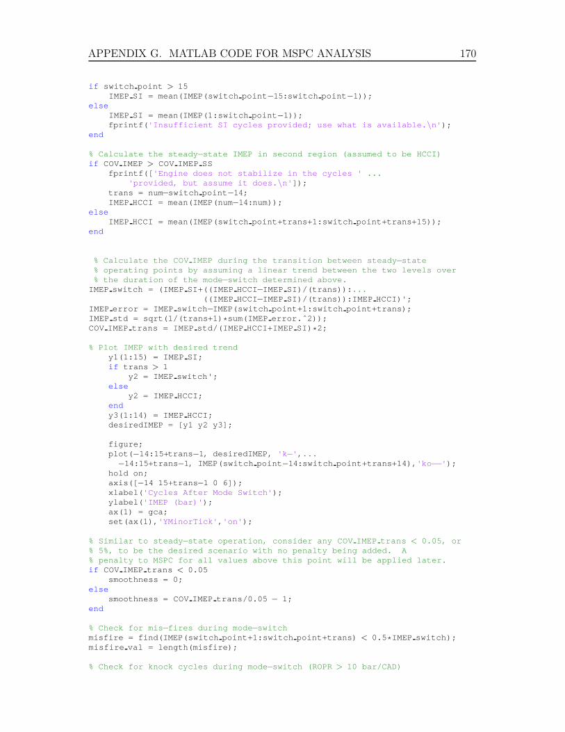
APPENDIX G. MATLAB CODE FOR MSPC ANALYSIS 170
if switch point > 15IMEP SI = mean(IMEP(switch point −15:switch point −1));
elseIMEP SI = mean(IMEP(1:switch point −1));fprintf( 'Insufficient SI cycles provided; use what is available. \n' );
end
% Calculate the steady −state IMEP in second region (assumed to be HCCI)if COVIMEP > COVIMEP SS
fprintf([ 'Engine does not stabilize in the cycles ' ...'provided, but assume it does. \n' ]);
trans = num −switch point −14;IMEP HCCI = mean(IMEP(num−14:num));
elseIMEP HCCI = mean(IMEP(switch point+trans+1:switch point+trans+15));
end
% Calculate the COV IMEP during the transition between steady −state% operating points by assuming a linear trend between the two levels over% the duration of the mode −switch determined above.
IMEP switch = (IMEP SI+((IMEP HCCI−IMEP SI)/(trans)): ...((IMEP HCCI−IMEP SI)/(trans)):IMEP HCCI)';
IMEP error = IMEP switch −IMEP(switch point+1:switch point+trans);IMEP std = sqrt(1/(trans+1) * sum(IMEP error.ˆ2));COVIMEP trans = IMEP std/(IMEP HCCI+IMEP SI) * 2;
% Plot IMEP with desired trendy1(1:15) = IMEP SI;if trans > 1
y2 = IMEP switch';else
y2 = IMEP HCCI;endy3(1:14) = IMEP HCCI;desiredIMEP = [y1 y2 y3];
figure;plot( −14:15+trans −1, desiredIMEP, 'k −' , ...
−14:15+trans −1, IMEP(switch point −14:switch point+trans+14), 'ko −−' );hold on;axis([ −14 15+trans −1 0 6]);xlabel( 'Cycles After Mode Switch' );ylabel( 'IMEP (bar)' );ax(1) = gca;set(ax(1), 'YMinorTick' , 'on' );
% Similar to steady −state operation, consider any COV IMEP trans < 0.05, or% 5%, to be the desired scenario with no penalty being added. A% penalty to MSPC for all values above this point will be appli ed later.if COVIMEP trans < 0.05
smoothness = 0;else
smoothness = COV IMEP trans/0.05 − 1;end
% Check for mis −fires during mode −switchmisfire = find(IMEP(switch point+1:switch point+trans) < 0.5 * IMEP switch);misfire val = length(misfire);
% Check for knock cycles during mode −switch (ROPR > 10 bar/CAD)
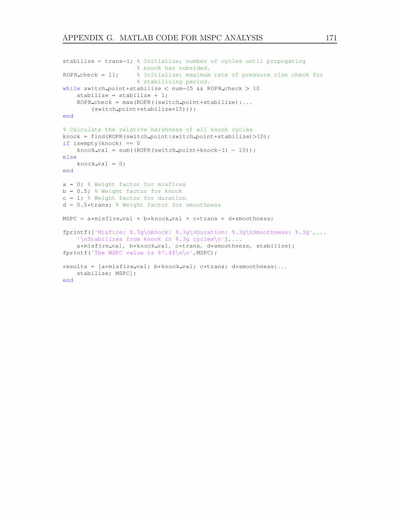
APPENDIX G. MATLAB CODE FOR MSPC ANALYSIS 171
stabilize = trans −1; % Initialize; number of cycles until propogating% knock has subsided.
ROPRcheck = 11; % Initialize; maximum rate of pressure rise check for% stabilizing period.
while switch point+stabilize < num−15 && ROPRcheck > 10stabilize = stabilize + 1;ROPRcheck = max(ROPR((switch point+stabilize): ...
(switch point+stabilize+15)));end
% Calculate the relative harshness of all knock cyclesknock = find(ROPR(switch point:switch point+stabilize) >10);if isempty(knock) == 0
knock val = sum((ROPR(switch point+knock −1) − 10));else
knock val = 0;end
a = 0; % Weight factor for misfiresb = 0.5; % Weight factor for knockc = 1; % Weight factor for durationd = 0.5 * trans; % Weight factor for smoothness
MSPC = a* misfire val + b * knock val + c * trans + d * smoothness;
fprintf([ 'Misfire: %.3g \nKnock: %.3g \nDuration: %.3g \nSmoothness: %.3g' , ...' \nStabilizes from knock in %.3g cycles \n' ], ...a* misfire val, b * knock val, c * trans, d * smoothness, stabilize);
fprintf( 'The MSPC value is %7.4f \n\n' ,MSPC);
results = [a * misfire val; b * knock val; c * trans; d * smoothness; ...stabilize; MSPC];
end
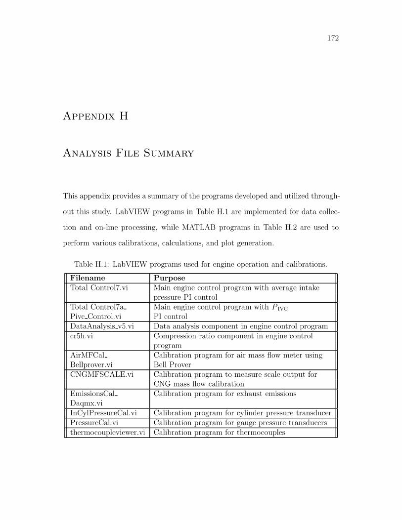
172
Appendix H
Analysis File Summary
This appendix provides a summary of the programs developed and utilized through-
out this study. LabVIEW programs in Table H.1 are implemented for data collec-
tion and on-line processing, while MATLAB programs in Table H.2 are used to
perform various calibrations, calculations, and plot generation.
Table H.1: LabVIEW programs used for engine operation and calibrations.
Filename PurposeTotal Control7.vi Main engine control program with average intake
pressure PI controlTotal Control7a Main engine control program with P IVC
Pivc Control.vi PI controlDataAnalysis v5.vi Data analysis component in engine control programcr5h.vi Compression ratio component in engine control
programAirMFCal Calibration program for air mass flow meter usingBellprover.vi Bell ProverCNGMFSCALE.vi Calibration program to measure scale output for
CNG mass flow calibrationEmissionsCal Calibration program for exhaust emissionsDaqmx.viInCylPressureCal.vi Calibration program for cylinder pressure transducerPressureCal.vi Calibration program for gauge pressure transducersthermocoupleviewer.vi Calibration program for thermocouples

APPENDIX H. ANALYSIS FILE SUMMARY 173
Table H.2: MATLAB programs used to process data and create figures.
Filename PurposeMS plot 7.m Generate plots for “intake pressure, CNG PW,
and IMEP”, “CNG injection timing”, and“CA50 and ROPR”
MS plot indiv 7.m Generate plots of intake pressure, CNG PW,IMEP, CNG injection timing, CA50, ROPR,and equivalence ratio
SI HCCI MSPC 7.m Analysis file for Mode-SwitchingPerformance Criterion
air cng Generate plots for characterizing CNG injectorcharacterization.mcal plot print.m Converts MATLAB plots to .eps formatCFR timing plot.m Generate index plots for Figure F.1intake pressure Generate plots of intake pressure andplot.m air mass flow ratePivcPlot.m Generate plots for P IVC samples and pressure
measurements upstream/downstream of throttlethrottle nonlinear Generate plot for non-linear Woodward throttleplot.m trendAirMF import.m Import and organize air mass flow calibration dataAirMF Cal2.m Calibration processing for air mass flow meter dataAirMFplot.m Calibration plot for air mass flow metercngMFplot.m Calibration plot for CNG mass flow meterPressurePlots.m Calibration plot for gauge pressure transducersfile name Extract pressures and test number from filenameextract.m for cylinder pressure transducer calibration testspcal2.m Calibration processing for cylinder pressure transducerThermocouplePlot.m Calibration plot for thermocouples