Embed Size (px)
Citation preview
University of Alberta
Optimization of steam/solvent injection methods: Application of hybrid
techniques with improved algorithm configuration
by
Muhammad Mugren Algosayir
A thesis submitted to the Faculty of Graduate Studies and Research
in partial fulfillment of the requirements for the degree of
Master of Science in
Petroleum Engineering
Department of Civil and Environmental Engineering
©Muhammad Mugren Algosayir
Fall 2012
Edmonton, Alberta
Permission is hereby granted to the University of Alberta Libraries to reproduce single copies of this thesis
and to lend or sell such copies for private, scholarly or scientific research purposes only. Where the thesis is
converted to, or otherwise made available in digital form, the University of Alberta will advise potential users
of the thesis of these terms.
The author reserves all other publication and other rights in association with the copyright in the thesis and,
except as herein before provided, neither the thesis nor any substantial portion thereof may be printed or
otherwise reproduced in any material form whatsoever without the author's prior written permission.

I dedicate this work to Allah, and then to my parents, Mugren and Meznah, and my wife Manahel
who always motivate and encourage me toward the success with their countless support

Abstract
Heavy oil and bitumen recovery processes need to be optimized in order to increase the recovery,
reduce costs, and minimize the environment impact. Most of the optimization studies published in
petroleum engineering literature focus on a few design parameters by combining the elements of
numerical flow simulation with graphical or analytical techniques. Limited efforts, particularly in
the areas of enhanced heavy oil recovery design, combine global optimization techniques with
flow simulation to achieve better performance and design. The challenge remains because of high
computational costs and slow convergence efficiency of the algorithms. In this research, genetic
algorithm and simulated annealing are considered first as a single optimization technique. Then,
the hybridization of these with the orthogonal arrays and response surface proxy techniques are
tested. Savings up to 85% on the execution time are obtained for steam and solvent applications in
oilsands and fractured carbonates.

Acknowledgements
Usually you do not realize the wisdom behind advice of the people who experienced life until you
do them. I will never forget the encouragements and motivations of my parents, Mugren and
Meznah, to excel in my study, and the words would not express my gratitude toward them. In
addition, I do not forget Waleed Al-Awadh who supported and encouraged me to pursue my
master in petroleum engineering. Special appreciations for my advisors Dr. Tayfun Babadagli and
Dr. Juliana Leung for their support and advice that made this work see the lights. In addition, I
would like to acknowledge Abo Sagr who simplified petroleum engineering learning for me. The
wonderful time during my study would not be possible without my wife Manahel who always does
the best. Finally, I would like to thank Saudi Aramco for providing the scholarship for my MSc
study at the University of Alberta specially Claire Cardwell who coached me during my training
assignment (Ch. 14).
A partial support for this research was obtained from Dr. Tayfun Babadagli’s NSERC Industrial
Research Chair in Unconventional Oil Recovery (industrial partners are Schlumberger, CNRL,
SUNCOR, Petrobank, Sherritt Oil, and APEX Eng.). In addition, this research was partially
supported by Dr. Juliana Leung’s "NSERC Discovery Grant".
Table of Contents
Chapter 1: Introduction ................................................................................................................ 1
Nomenclature ............................................................................................................................... 2
References .................................................................................................................................... 2
Chapter 2: Problem Statement & Research Objectives ................................................................ 3
Chapter 3: Solution Methodology ................................................................................................ 4
Global Optimization Techniques ................................................................................................. 4
Genetic Algorithm ................................................................................................................... 5
GA Advantages .................................................................................................................... 7
GA Disadvantages ................................................................................................................ 7
GA Accelerators ................................................................................................................... 7
Simulated Annealing ............................................................................................................. 10
Research optimization framework ............................................................................................. 11
JGAP Runner for initialization and executing ....................................................................... 11
CMG Agents package ............................................................................................................ 12
Response surface proxy package ........................................................................................... 12
Nearly Orthogonal Arrays (NOA) reader package ................................................................ 12
Nomenclature ............................................................................................................................. 13
References .................................................................................................................................. 14
Chapter 4: Optimization of SAGD and Solvent Additive SAGD Applications: Comparative
Analysis of Optimization Techniques with Improved Algorithm Configuration ........................... 15
Abstract ...................................................................................................................................... 15
Introduction ................................................................................................................................ 16
Global Optimization Techniques ............................................................................................... 17
Genetic Algorithm ................................................................................................................. 17
Advantages ......................................................................................................................... 17
Disadvantages ..................................................................................................................... 18
GA Accelerators ................................................................................................................. 18
Simulated Annealing ............................................................................................................. 18
Objective function ...................................................................................................................... 19
Reservoir model ......................................................................................................................... 19
Results ........................................................................................................................................ 20
Genetic Algorithm Case 1 (GA 1) ......................................................................................... 20
Simulated Annealing case (SA) ............................................................................................. 20
Optimized Genetic Algorithm Cases (OGA 1) ...................................................................... 20
Hexane Additive SAGD Case (HA-GA) ............................................................................... 21
Conclusions ................................................................................................................................ 22
Nomenclature ............................................................................................................................. 23
References .................................................................................................................................. 24
Tables ......................................................................................................................................... 26
Figures ....................................................................................................................................... 29
Chapter 5: Design of Solvent-Assisted SAGD Processes in Heterogeneous Reservoirs Using
Hybrid Optimization Techniques ................................................................................................... 33
Abstract ...................................................................................................................................... 33
Introduction ................................................................................................................................ 34
Methodology .............................................................................................................................. 34
Global Optimization Techniques ........................................................................................... 34
Orthogonal Array and Nearly-Orthogonal Array for Initial Population Generation .............. 35
Proxy Method for Objective Function Evaluation ................................................................. 35
Objective Function ..................................................................................................................... 36
Case Study ................................................................................................................................. 37
Model Description ................................................................................................................. 37
Response Surface Proxy Models ................................................................................................ 37
Results and Discussion ............................................................................................................... 37
Conclusions ................................................................................................................................ 40
Nomenclature ............................................................................................................................. 41
Tables ......................................................................................................................................... 43
Figures ....................................................................................................................................... 47
Chapter 6: Optimization of SOS-FR (Steam-Over-Solvent Injection in Fractured Reservoirs)
Method Using Hybrid Techniques: Testing Cyclic Injection Case ............................................... 55
Abstract ...................................................................................................................................... 55
Introduction ................................................................................................................................ 55
Optimization methodology......................................................................................................... 57
Global Optimization Techniques ........................................................................................... 57
Orthogonal Arrays for Experimental Design ......................................................................... 58
Proxy Method for Objective Function Evaluation with Periodic Updating ........................... 58
Objective Function ................................................................................................................ 59
Benchmark (Base) Simulation Model ........................................................................................ 60
Results and Discussion ............................................................................................................... 61
Experiment 1: ........................................................................................................................ 61
Experiment 2: ........................................................................................................................ 62
Experiment 3: ........................................................................................................................ 62
Experiment 4: ........................................................................................................................ 62
Conclusions and remarks ........................................................................................................... 64
Nomenclature ............................................................................................................................. 65
References .................................................................................................................................. 67
Tables ......................................................................................................................................... 69
Figures ....................................................................................................................................... 72
Chapter 7: Contributions ............................................................................................................ 78

Appendix 1: JGAP initializer code ........................................................................................... 79
Appendix 2: Objective function evaluation code ...................................................................... 84
Appendix 3: CMG Agents Package .......................................................................................... 87
Appendix 4: Response surface proxy package .......................................................................... 98
Appendix 5: NOA reading package ........................................................................................ 102
List of Tables
Table 3-1: Nearly orthogonal array example .................................................................................... 7
Table 4-1: Reservoir simulation input parameters. ......................................................................... 26
Table 4-2: Optimized parameters ranges. ....................................................................................... 26
Table 4-3: NOA Tables. ................................................................................................................. 27
Table 4-4: Simulated annealing configuration. .............................................................................. 27
Table 4-5: GA cases configuration. ................................................................................................ 28
Table 4-6: Comparison of the selected solution. ............................................................................ 28
Table 4-7: Optimized Hexane Mole Fraction. ................................................................................ 28
Table 5-1:Optimizedparameters’ranges....................................................................................... 43
Table 5-2: GA configuration .......................................................................................................... 43
Table 5-3: Reservoir simulation input parameters .......................................................................... 43
Table 5-4: Nearly-Orthogonal Array (6 factors, 17 levels, and 30 runs) used for generating initial
population ....................................................................................................................................... 44
Table 5-5: Comparison of the selected solution values .................................................................. 45
Table 5-6: Cases execution time ..................................................................................................... 46
Table 6-1: Elements prices ............................................................................................................. 69
Table 6-2: Reservoir properties used in the simulations. ................................................................ 69
Table 6-3:Optimizedparameters’ranges....................................................................................... 69
Table 6-4: Optimal parameters values for all experiments. ............................................................ 70
Table 6-5: Optimal lengths indicators of the base case, experiment 1, 2, and 3. ............................ 70
Table 6-6: Comparison of the selected solution values .................................................................. 70
Table 6-7: Experiments huff-and-puff phases lengths in days ....................................................... 71
List of Figures
Figure 3-1: Optimization algorithms classification .......................................................................... 4
Figure 3-2: Schematic representation of optimization process. ........................................................ 5
Figure 3-3: Optimization process in genetic algorithm terminology ................................................ 5
Figure 3-4: Genetic algorithm flow diagram .................................................................................... 6
Figure 3-5: Example of crossover of two parent chromosomes. ...................................................... 6
Figure 3-6: Example of mutation of a parent chromosome. ............................................................. 6
Figure 3-7: Flow diagram for the periodic updating approach where proxy is updated with the
additional flow simulation results of the fittest chromosomes after each evolution ......................... 9
Figure 3-8: Simulated annealing one iteration flow chart .............................................................. 10
Figure 3-9: Optimization framework packages interaction. ........................................................... 11
Figure 4-1: Schematic representation of optimization process. ...................................................... 29
Figure 4-2: Optimization process in Genetic Algorithm terminology. ........................................... 29
Figure 4-3: Genetic Algorithm flow diagram. ................................................................................ 30
Figure 4-4: Example of crossover of two parent chromosomes. .................................................... 30
Figure 4-5: Example of mutation of a parent chromosome. ........................................................... 30
Figure 4-6: Function value for the GA with different ways of generating initial population. ........ 31
Figure 4-7: Convergence speed comparison between SA and Optimized GA case. ...................... 31
Figure 4-8: Simulated Annealing (SA) function value (F(X)) and injection rates (X values). ....... 32
Figure 4-9: Optimized Genetic Algorithm Case 1 (OGA-1) function value (F(X)) and injection
rates (X values). .............................................................................................................................. 32
Figure 5-1: Conventional Genetic Algorithm flow diagram (modified from Algosayir et al. 2011).
........................................................................................................................................................ 47
Figure 5-2: 30% shale sand distribution. ........................................................................................ 47
Figure 5-3: 10% shale sand distribution. ........................................................................................ 48
Figure 5-4: Optimized ES-SAGD homogeneous case oil production profile. ................................ 48
Figure 5-5: Proxies approximation for the homogeneous case: trials are sorted based on actual
flow simulation fitness value J. ...................................................................................................... 49
Figure 5-6: Proxy approximation for the 30% shale case. .............................................................. 49
Figure 5-7: Proxy approximation for the 10% shale case. .............................................................. 50
Figure 5-8: Fitness value as a function of evolution for the homogeneous case. ........................... 50
Figure 5-9: Fitness value as a function of evolution for the 30% shale case. ................................. 51
Figure 5-10: Fitness value as a function of evolution for the 10% shale case. ............................... 51
Figure 5-11: Flow diagram for the modified approach where proxy is updated with the additional
flow simulation results of the fittest chromosomes after each evolution. ....................................... 52
Figure 5-12: Fitness value as a function of evolution for the homogeneous case using the modified
approach with non-linear proxy updating. ...................................................................................... 53
Figure 5-13: Fitness value as a function of evolution for the 30% shale case using the modified
approach with non-linear proxy updating. ...................................................................................... 53
Figure 5-14: Fitness value as a function of evolution for the 10% shale case using the modified
approach with non-linear proxy updating. ...................................................................................... 54
Figure 6-1: Conventional genetic algorithm flow diagram............................................................. 72
Figure 6-2: Example of crossover of two parent chromosomes. .................................................... 72
Figure 6-3: Example of mutation of a parent chromosome. ........................................................... 72
Figure 6-4: Flow diagram for the modified approach where proxy is updated with the additional
flow simulation results of the fittest chromosomes after each evolution. ....................................... 73
Figure 6-5: Representation of multiple-matrix block with unity oil saturation in flow simulation.
........................................................................................................................................................ 74
Figure 6-6: Sensitivity analysis for some key parameters before starting the optimization. .......... 74
Figure 6-7: Optimized money recovery factor, oil recovery factor, and cumulative steam oil ratio
of all experiment. ............................................................................................................................ 75
Figure 6-8: Optimized cost, revenue and profit of all experiments. ............................................... 75
Figure 6-9: All experiments hydrocarbons and steam injected and produced. ............................... 76
Figure 6-10: Base case Gantt-chart ................................................................................................ 76

Figure 6-11: Experiment 4-d (best MRF) Gantt-chart. ................................................................... 77
Figure 6-12: Experiment 4-b (random initial population) Gantt-chart. .......................................... 77
1
Chapter 1: Introduction
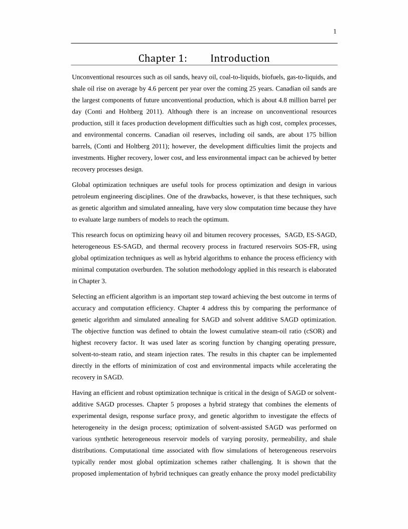
Unconventional resources such as oil sands, heavy oil, coal-to-liquids, biofuels, gas-to-liquids, and
shale oil rise on average by 4.6 percent per year over the coming 25 years. Canadian oil sands are
the largest components of future unconventional production, which is about 4.8 million barrel per
day (Conti and Holtberg 2011). Although there is an increase on unconventional resources
production, still it faces production development difficulties such as high cost, complex processes,
and environmental concerns. Canadian oil reserves, including oil sands, are about 175 billion
barrels, (Conti and Holtberg 2011); however, the development difficulties limit the projects and
investments. Higher recovery, lower cost, and less environmental impact can be achieved by better
recovery processes design.
Global optimization techniques are useful tools for process optimization and design in various
petroleum engineering disciplines. One of the drawbacks, however, is that these techniques, such
as genetic algorithm and simulated annealing, have very slow computation time because they have
to evaluate large numbers of models to reach the optimum.
This research focus on optimizing heavy oil and bitumen recovery processes, SAGD, ES-SAGD,
heterogeneous ES-SAGD, and thermal recovery process in fractured reservoirs SOS-FR, using
global optimization techniques as well as hybrid algorithms to enhance the process efficiency with
minimal computation overburden. The solution methodology applied in this research is elaborated
in Chapter 3.
Selecting an efficient algorithm is an important step toward achieving the best outcome in terms of
accuracy and computation efficiency. Chapter 4 address this by comparing the performance of
genetic algorithm and simulated annealing for SAGD and solvent additive SAGD optimization.
The objective function was defined to obtain the lowest cumulative steam-oil ratio (cSOR) and
highest recovery factor. It was used later as scoring function by changing operating pressure,
solvent-to-steam ratio, and steam injection rates. The results in this chapter can be implemented
directly in the efforts of minimization of cost and environmental impacts while accelerating the
recovery in SAGD.
Having an efficient and robust optimization technique is critical in the design of SAGD or solvent-
additive SAGD processes. Chapter 5 proposes a hybrid strategy that combines the elements of
experimental design, response surface proxy, and genetic algorithm to investigate the effects of
heterogeneity in the design process; optimization of solvent-assisted SAGD was performed on
various synthetic heterogeneous reservoir models of varying porosity, permeability, and shale
distributions. Computational time associated with flow simulations of heterogeneous reservoirs
typically render most global optimization schemes rather challenging. It is shown that the
proposed implementation of hybrid techniques can greatly enhance the proxy model predictability
2
and computational efficiency. Hexane was co-injected with steam. The objective function, defined
based on cumulative steam-oil ratio (cSOR) and recovery factor, was optimized by changing
injection pressures, production pressures, and injected solvent-to-steam ratio. The results from
these hybrid approaches revealed that an optimized solution could be achieved with less CPU time
(e.g. fewer number of full flow simulation) compared to the conventional GA method. Sensitivity
analysis was also conducted on the choice of proxy model to study the robustness of the proposed
methods. Our results highlight the potential application of the proposed techniques in other
solvent-enhanced heavy oil recovery processes.
Chapter 6 focuses on optimizing Steam-Over-Solvent Injection for Fractured Reservoirs (SOS-FR)
process using a hybrid technique applied in Chapter 5. The complexity of the process suggests that
our objective function, defined by the money recovery factor, can be increased significantly by
adjusting the steam and solvent usage and their injection profiles.
As this is a paper-based thesis, each chapter contains its own literature review, conclusion and
references. The major contributions of this research are highlighted in Chapter 7.
Nomenclature
ES-SAGD: Expanded solvent steam assisted gravity drainage thermal recovery process also
known as solvent additive SAGD.
GA: Genetic Algorithm.
NOA: Nearly-Orthogonal Array.
OA: Orthogonal Array.
SAGD: Steam assisted gravity drainage thermal recovery process.
SOS-FR: Steam-Over-Solvent for Fractured Reservoirs.
References
Conti J., and Holtberg P. 2011. International Energy Outlook 2011. A report published in U.S. Energy
Information Administration. http://www.eia.gov/forecasts/ieo/pdf/0484(2011).pdf
3
Chapter 2: Problem Statement & Research Objectives
In order to reach the ultimate heavy oil and bitumen recovery with minimal cost, efficient and
optimized design for recovery processes operation strategies is necessary. Despite huge amount of
heavy oil and bitumen reserves around the world, the production is limited due to the production
development difficulties such as high cost, complex processes, and environmental concerns. Many
design and performance evaluation studies published in the literature combine numerical
simulation with graphical or analytical techniques; however, only few design elements are handled
due to the difficulties of handling large number of factors. Because of high computation
requirements, limited attention that integrated the simulation exercise with global optimization
algorithms has been paid to handle more design elements. Without efficient and optimized
recovery process design, the ultimate recovery from unconventional resources will not be
achieved, or it could be achieved with great cost and large environmental impact. Thus, this
research studies how global optimization techniques can be enhanced and upgraded to be a robust
tool for the design and performance evaluation of unconventional recovery processes.
The objective of this research is to develop an approach that combines the techniques of
experimental design, proxy models, and global optimization for the design of key process elements
in the thermal/solvent methods. It is well known that computing costs associated with flow
simulation of complex recovery processes (solvent and steam injection) in heterogeneous
reservoirs can pose significant challenges on the optimization procedure. The use of hybrid
techniques, as implemented in this thesis, aims to minimize the computational costs and to
improve the solution accuracy.
4
Chapter 3: Solution Methodology
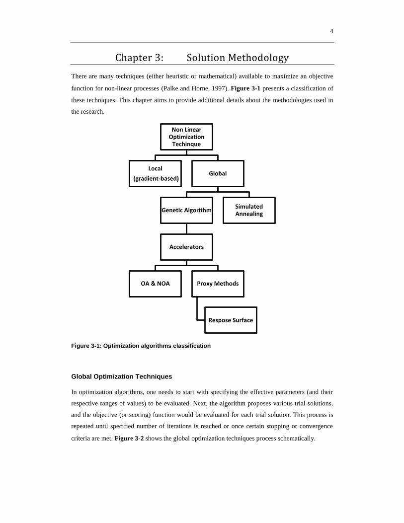
There are many techniques (either heuristic or mathematical) available to maximize an objective
function for non-linear processes (Palke and Horne, 1997). Figure 3-1 presents a classification of
these techniques. This chapter aims to provide additional details about the methodologies used in
the research.
Figure 3-1: Optimization algorithms classification
Global Optimization Techniques
In optimization algorithms, one needs to start with specifying the effective parameters (and their
respective ranges of values) to be evaluated. Next, the algorithm proposes various trial solutions,
and the objective (or scoring) function would be evaluated for each trial solution. This process is
repeated until specified number of iterations is reached or once certain stopping or convergence
criteria are met. Figure 3-2 shows the global optimization techniques process schematically.
Non Linear Optimization
Techinque
Local
(gradient-based) Global
Genetic Algorithm
Accelerators
OA & NOA Proxy Methods
Respose Surface
Simulated Annealing
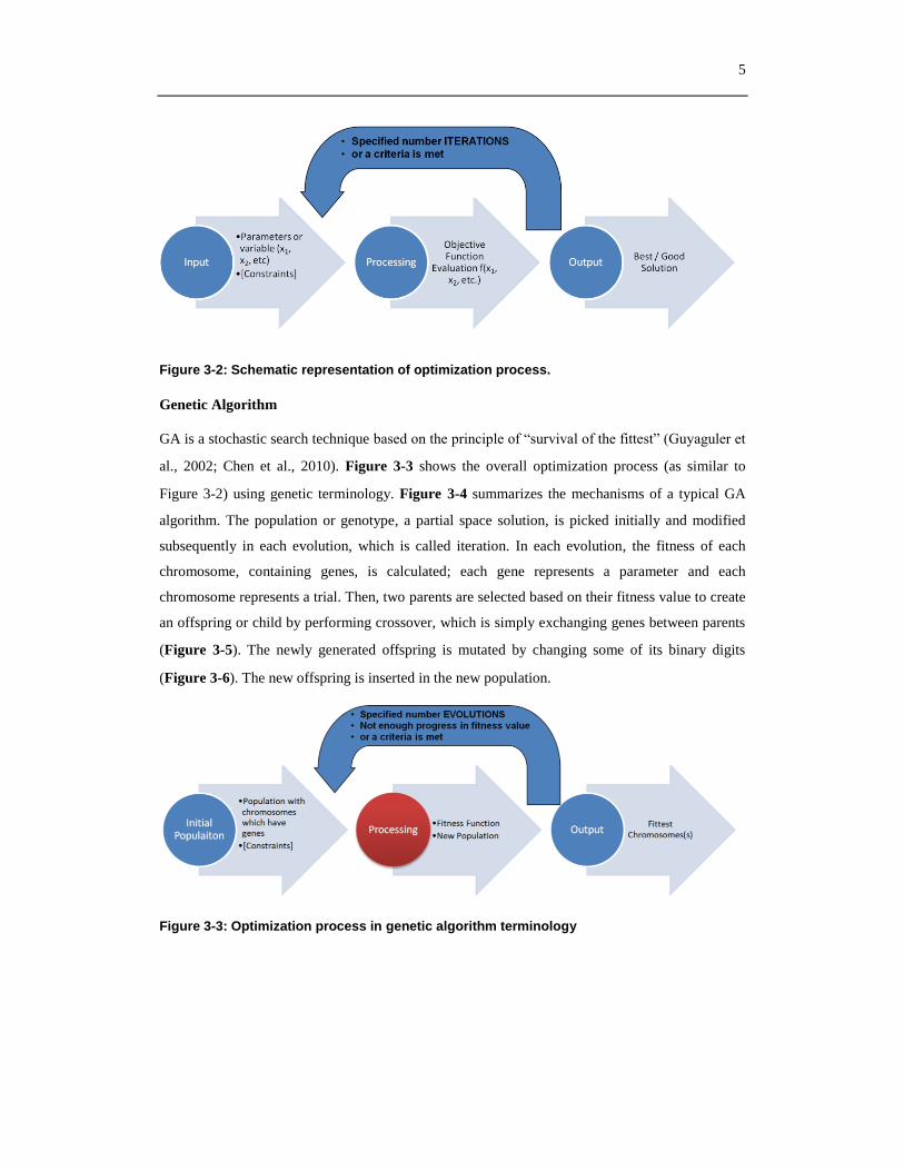
5
Figure 3-2: Schematic representation of optimization process.
Genetic Algorithm
GA is a stochastic search technique basedontheprincipleof“survivalofthefittest”(Guyaguleret
al., 2002; Chen et al., 2010). Figure 3-3 shows the overall optimization process (as similar to
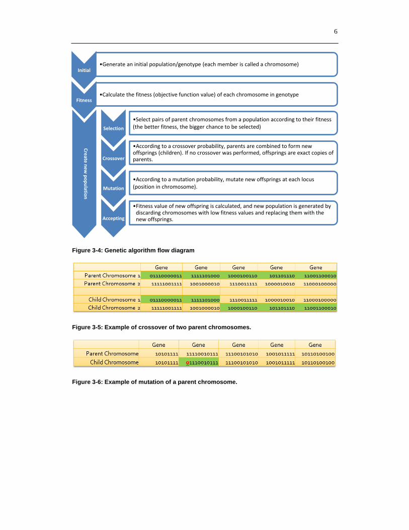
Figure 3-2) using genetic terminology. Figure 3-4 summarizes the mechanisms of a typical GA
algorithm. The population or genotype, a partial space solution, is picked initially and modified
subsequently in each evolution, which is called iteration. In each evolution, the fitness of each
chromosome, containing genes, is calculated; each gene represents a parameter and each
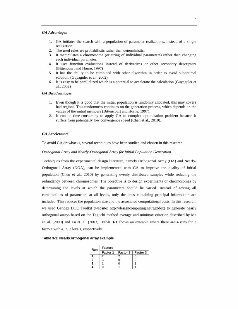
chromosome represents a trial. Then, two parents are selected based on their fitness value to create
an offspring or child by performing crossover, which is simply exchanging genes between parents
(Figure 3-5). The newly generated offspring is mutated by changing some of its binary digits
(Figure 3-6). The new offspring is inserted in the new population.
Figure 3-3: Optimization process in genetic algorithm terminology
6
Figure 3-4: Genetic algorithm flow diagram
Figure 3-5: Example of crossover of two parent chromosomes.
Figure 3-6: Example of mutation of a parent chromosome.
Initial •Generate an initial population/genotype (each member is called a chromosome)
Fitness •Calculate the fitness (objective function value) of each chromosome in genotype
Selection
•Select pairs of parent chromosomes from a population according to their fitness (the better fitness, the bigger chance to be selected)
Crossover
•According to a crossover probability, parents are combined to form new offsprings (children). If no crossover was performed, offsprings are exact copies of parents.
Mutation
•According to a mutation probability, mutate new offsprings at each locus (position in chromosome).
Accepting
•Fitness value of new offspring is calculated, and new population is generated by discarding chromosomes with low fitness values and replacing them with the new offsprings.
Cre
ate n
ew p
op
ulatio
n
7
GA Advantages
1. GA initiates the search with a population of parameter realizations, instead of a single
realization.
2. The used rules are probabilistic rather than deterministic.
3. It manipulates a chromosome (or string of individual parameters) rather than changing
each individual parameter.
4. It uses function evaluations instead of derivatives or other secondary descriptors
(Bittencourt and Horne, 1997)
5. It has the ability to be combined with other algorithm in order to avoid suboptimal
solution. (Guyaguler et al., 2002)
6. It is easy to be parallelized which is a potential to accelerate the calculation (Guyaguler et
al., 2002)
GA Disadvantages
1. Even though it is good that the initial population is randomly allocated, this may covers
bad regions. This randomness continues on the generation process, which depends on the
values of the initial members (Bittencourt and Horne, 1997).
2. It can be time-consuming to apply GA to complex optimization problem because it
suffers from potentially low convergence speed (Chen et al., 2010).
GA Accelerators
To avoid GA drawbacks, several techniques have been studied and chosen in this research.
Orthogonal Array and Nearly-Orthogonal Array for Initial Population Generation
Techniques from the experimental design literature, namely Orthogonal Array (OA) and Nearly-
Orthogonal Array (NOA), can be implemented with GA to improve the quality of initial
population (Chen et al., 2010) by generating evenly distributed samples while reducing the
redundancy between chromosomes. The objective is to design experiments or chromosomes by
determining the levels at which the parameters should be varied. Instead of testing all
combinations of parameters at all levels, only the ones containing principal information are
included. This reduces the population size and the associated computational costs. In this research,
we used Gendex DOE Toolkit (website: http://designcomputing.net/gendex) to generate nearly
orthogonal arrays based on the Taguchi method average and minimax criterion described by Ma
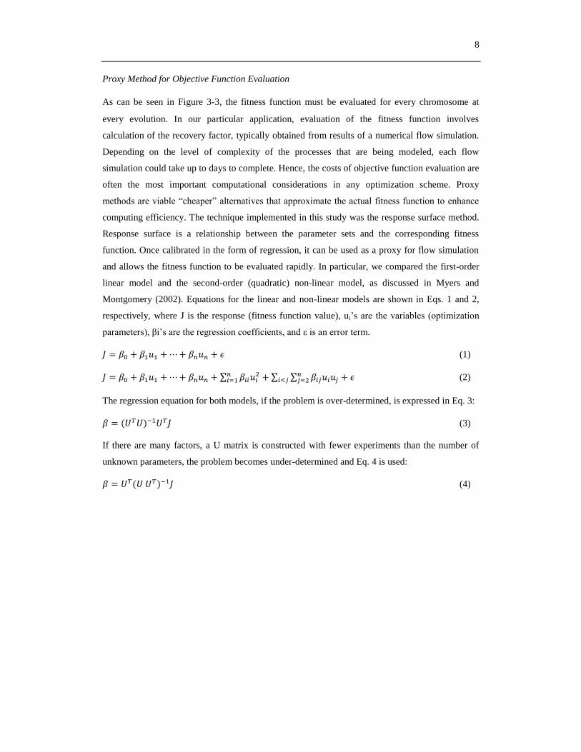
et. al. (2000) and Lu et. al. (2003). Table 3-1 shows an example where there are 4 runs for 3
factors with 4, 3, 2 levels, respectively.
Table 3-1: Nearly orthogonal array example
Run Factors
Factor 1 Factor 2 Factor 3
1 2 2 0 2 3 0 0 3 1 0 1 4 0 1 1
8
Proxy Method for Objective Function Evaluation
As can be seen in Figure 3-3, the fitness function must be evaluated for every chromosome at
every evolution. In our particular application, evaluation of the fitness function involves
calculation of the recovery factor, typically obtained from results of a numerical flow simulation.
Depending on the level of complexity of the processes that are being modeled, each flow
simulation could take up to days to complete. Hence, the costs of objective function evaluation are
often the most important computational considerations in any optimization scheme. Proxy
methodsareviable“cheaper”alternativesthatapproximatetheactualfitnessfunctiontoenhance
computing efficiency. The technique implemented in this study was the response surface method.
Response surface is a relationship between the parameter sets and the corresponding fitness
function. Once calibrated in the form of regression, it can be used as a proxy for flow simulation
and allows the fitness function to be evaluated rapidly. In particular, we compared the first-order
linear model and the second-order (quadratic) non-linear model, as discussed in Myers and
Montgomery (2002). Equations for the linear and non-linear models are shown in Eqs. 1 and 2,
respectively, where J is the response (fitness function value), ui’sare thevariables(optimization
parameters),βi’saretheregressioncoefficients,andεisanerrorterm.
(1)
∑
∑ ∑ (2)
The regression equation for both models, if the problem is over-determined, is expressed in Eq. 3:
(3)
If there are many factors, a U matrix is constructed with fewer experiments than the number of
unknown parameters, the problem becomes under-determined and Eq. 4 is used:
(4)
9
Proxy Method for Objective Function Evaluation with Periodic Updating
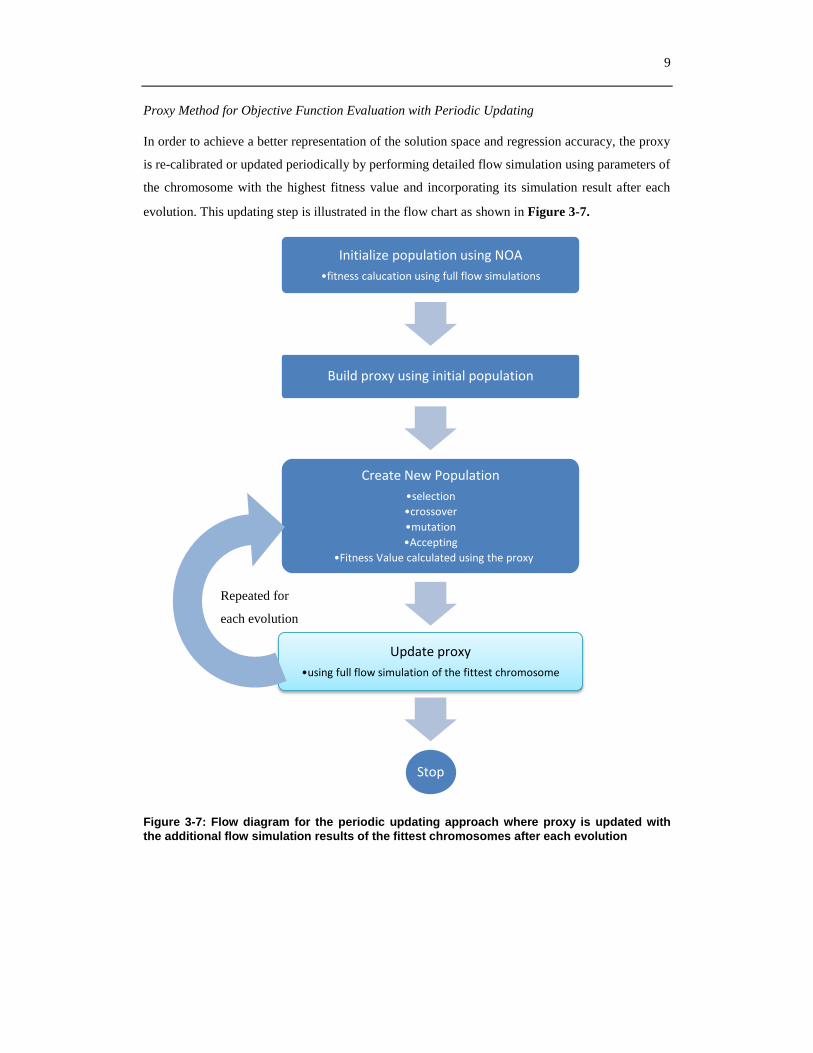
In order to achieve a better representation of the solution space and regression accuracy, the proxy
is re-calibrated or updated periodically by performing detailed flow simulation using parameters of
the chromosome with the highest fitness value and incorporating its simulation result after each
evolution. This updating step is illustrated in the flow chart as shown in Figure 3-7.
Figure 3-7: Flow diagram for the periodic updating approach where proxy is updated with
the additional flow simulation results of the fittest chromosomes after each evolution
Initialize population using NOA
•fitness calucation using full flow simulations
Build proxy using initial population
Create New Population
•selection
•crossover
•mutation
•Accepting
•Fitness Value calculated using the proxy
Update proxy
•using full flow simulation of the fittest chromosome
Stop
Repeated for
each evolution
10
Simulated Annealing
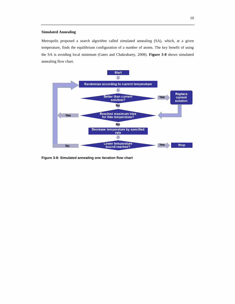
Metropolis proposed a search algorithm called simulated annealing (SA), which, at a given
temperature, finds the equilibrium configuration of a number of atoms. The key benefit of using
the SA is avoiding local minimum (Gates and Chakrabarty, 2008). Figure 3-8 shows simulated
annealing flow chart.
Figure 3-8: Simulated annealing one iteration flow chart
11
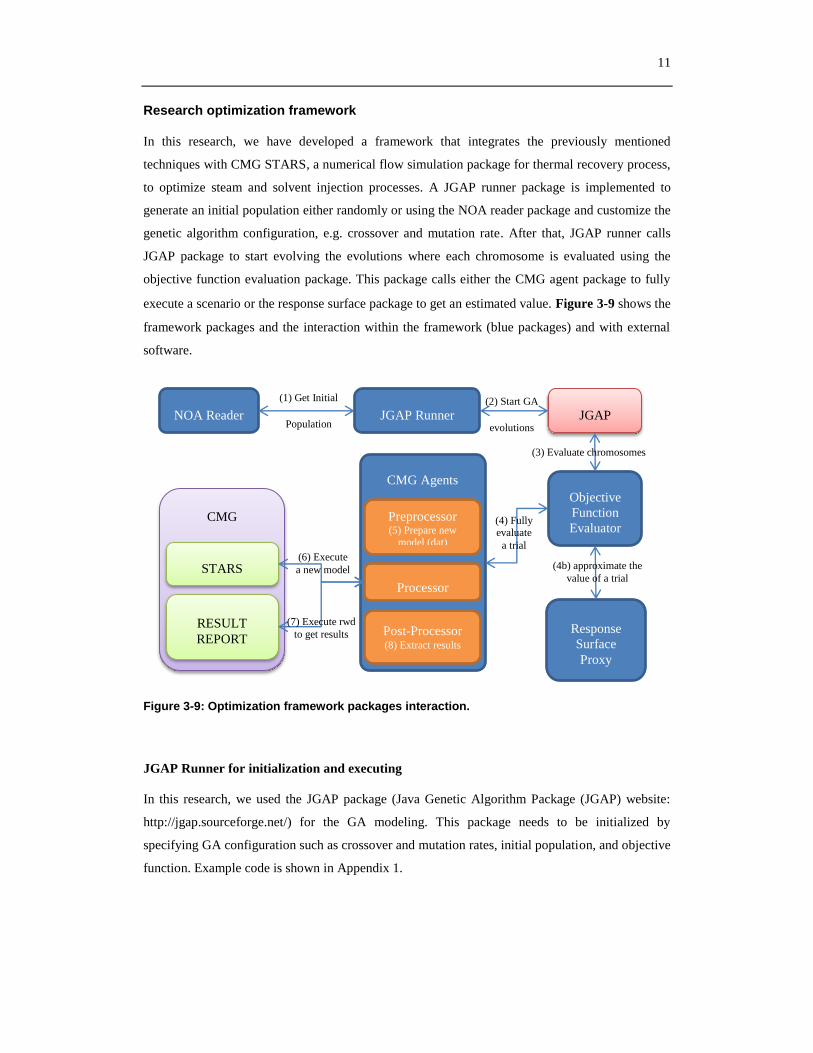
Research optimization framework
In this research, we have developed a framework that integrates the previously mentioned
techniques with CMG STARS, a numerical flow simulation package for thermal recovery process,
to optimize steam and solvent injection processes. A JGAP runner package is implemented to
generate an initial population either randomly or using the NOA reader package and customize the
genetic algorithm configuration, e.g. crossover and mutation rate. After that, JGAP runner calls
JGAP package to start evolving the evolutions where each chromosome is evaluated using the
objective function evaluation package. This package calls either the CMG agent package to fully
execute a scenario or the response surface package to get an estimated value. Figure 3-9 shows the
framework packages and the interaction within the framework (blue packages) and with external
software.
Figure 3-9: Optimization framework packages interaction.
JGAP Runner for initialization and executing
In this research, we used the JGAP package (Java Genetic Algorithm Package (JGAP) website:
http://jgap.sourceforge.net/) for the GA modeling. This package needs to be initialized by
specifying GA configuration such as crossover and mutation rates, initial population, and objective
function. Example code is shown in Appendix 1.
JGAP JGAP Runner
CMG
STARS
RESULT
REPORT
CMG Agents
Preprocessor (5) Prepare new
model (dat)
Processor
Post-Processor (8) Extract results
NOA Reader
(1) Get Initial
Population
(2) Start GA
evolutions
Objective
Function
Evaluator
(3) Evaluate chromosomes
(4) Fully evaluate
a trial
Response
Surface
Proxy
(4b) approximate the
value of a trial
(6) Execute
a new model
(7) Execute rwd
to get results

12
Objective function evaluation package
Global optimization techniques rely mainly on objective function evaluation for the generated
trials. In our framework, this package is responsible about calling the CMG Agent package to get
the results that are needed in the objective function calculation. Example code from SOS-FR
experiments is shown in Appendix 2.
CMG Agents package
This package handles the interaction between our software and CMG products. It has three stages
pre-processing, processing, and post post-processing. Pre-processing is needed to build a new
simulation model file (.dat) using old model file by changing the parts that need to be changed
using the values provided by the optimization algorithm. In the processing stage, the simulation is
executed. Post-processing stage extracts the relevant results from a *.rwo file, which is built by
executing the *.rwd file generated using CMG “Result Report” tool. Example code from SOS-FR
experiments is shown in Appendix 3.
Response surface proxy package
This package is used to build and calibrate the linear and non-linear proxy described before to
approximate the objective function. This package code is shown in Appendix 4.
Nearly Orthogonal Arrays (NOA) reader package
In this research, we used Gendex DOE Toolkit (website: http://designcomputing.net/gendex) to
generate the NOA arrays. This tool generates numbers that represent the level at which each factor
(parameter) should be used in a particular trial. These numbers must be converted to values
appropriate for the parameter ranges. For example, for injection rate ranging from 100 to 300
units, five levels, indicated by 0, 1, 2, 3, and 4, would correspond to actual parameter values of
100, 150, 200, 250, and 300 units, providing a 50-unit resolution for the parameter. This step can
be done manually using excel spreadsheet. After that, the newly generated OA is copied into a text
file to be read using this reader package. Example code from SOS-FR experiments is shown in
Appendix 5.

13
Nomenclature
βi : represent a regression coefficients for one trial.
: a vector which contains all regression coefficients.
F(u) or FX: objective function value.
F: objective function.
GA: Genetic Algorithm.
J: the actual response or actual objective function value calculated based simulation output for
one trial.
J’: the repose obtained from the regression model.
J0: the best trial actual response in the initial population.
: a vector that contains all the trials response.
NOA: Nearly-Orthogonal Array.
OA: Orthogonal Array.
SOS-FR: Steam-Over-Solvent for Fractured Reservoirs.
u: a (1*n) vector which contains the optimization variables for a trial.
ui : represent an optimization variable for one trial.
: a matrix with all u’s.
14
References
Palke, M.R., and Horne, R.N. 1997. Determining the Value of Reservoir Data by Using Nonlinear Production
Optimization Techniques. Paper SPE 38047 presented at the SPE Asia Pacific Oil and Gas Conference
and Exhibition, Kuala Lumpur, Malaysia, 14-16 April. DOI: 10.2118/38047-MS.
Gates, I.D., and Chakrabarty, N.. 2008. Design of the Steam and Solvent Injection Strategy in Expanding
Solvent Steam-Assisted Gravity Drainage. Journal of Canadian Petroleum Technology 47 (9): 12-20.
DOI: 10.2118/08-09-12-CS.
Guyaguler, B., Horne, R.N., Rogers, L., and Rosenzweig, J.J. 2002. Optimization of Well Placement in a
Gulf of Mexico Waterflooding Project. SPE Reservoir Evaluation & Engineering 5 (3): 229-236. DOI:
10.2118/78266-PA.
Chen, S., Li, H., Yang, D., and Tontiwachwuthikul, P. 2010. Optimal Parametric Design for Water-
Alternating-Gas (WAG) Process in a CO2-Miscible Flooding Reservoir. Journal of Canadian Petroleum
Technology 49 (10): 75-82. DOI: 10.2118/141650-PA.
Bittencourt, A.C., and Horne, R.N. 1997. Reservoir Development and Design Optimization. Paper 38895
presented at the SPE Annual Technical Conference and Exhibition, San Antonio, Texas, 5-8 October.
DOI: 10.2118/38895-MS.
Lu, X., Hu, W. & Zheng, Y. 2003. A Systematical Procedure in the Construction of Multi-Level
Supersaturated Designs. J. of Statistical Planning & Inference 115 (1): 287-310. DOI: 10.1016/S0378-
3758(02)00116-7.
Ma, C-X., Fang, K-T & Liski, E. 2000. A New Approach in Constructing Orthogonal and Nearly Orthogonal
Arrays. Metrika 50: 255-268. DOI: 10.1007/s001840050049.
Myers, R.H. and Montgomery D.C. 2002. Response Surface Methodology: Process and Product in
Optimization using Designed Experiments, Wily, New York.
15
A version of this chapter was submitted and accepted by Journal of Petroleum Science and Engineering and it is a revision
of the conference paper: Al-Gosayir, M., Babadagli, T., and Leung, J. 2011. Optimization of Solvent Additive SAGD Applications using Hybrid Optimization Techniques. Paper 144963 presented at the SPE Enhanced Oil Recovery
Conference, Kuala Lumpur, Malaysia, 19–21 July.
Chapter 4: Optimization of SAGD and Solvent Additive SAGD Applications: Comparative Analysis
of Optimization Techniques with Improved Algorithm Configuration
Abstract
Heavy oil and bitumen recovery cost is excessive mainly due to high energy requirement to
generate heat and its environmental impacts. Steam Assisted Gravity Drainage (SAGD) is an
example of this case. The determination of optimal operating conditions, such as injection rates
and well locations, based on reservoir and fluid characteristics is essential in the design of field
applications.
Many Steam Assisted Gravity Drainage (SAGD) optimization studies published in the literature
combined numerical simulation with graphical or analytical techniques for design and
performance evaluation. There have been limited efforts that integrated the simulation exercise
with global optimization algorithms. Some studies focused on optimization of cumulative steam-
to-oil ratio (cSOR) in SAGD by altering steam injection rates, while others focused on
optimization of cumulative net energy-to-oil ratio (cEOR) in solvent-additive SAGD by altering
injection pressures and fraction of solvent in the injection stream. Typical scoring functions were
the net present value per hectare of land (NPV/ha) by controlling steam and solvent rates. Several
studies also considered total project net present value calculation by changing total project area,
capital cost intensities, solvent prices, discount rate, and risk factors to determine the well spacing
and drilling schedule. Optimization techniques commonly used in those studies were scattered
search, simulated annealing, and genetic algorithm (GA). In continuation of these efforts, we
focused on optimizing the SAGD process and its extension to solvent-additive SAGD and several
optimization techniques including simulated annealing and genetic algorithm were tested and
compared. Additional procedures were incorporated to improve the implementation configuration
and initial population or seed. The objective function was defined to obtain the lowest cumulative
steam-oil ratio (cSOR) and highest recovery factor. It was used later as scoring function by
changing solvent-to-steam ratio and steam injection rates. The results in this chapter can be
implemented directly in the efforts of minimization of cost and environmental impacts while
accelerating the recovery in SAGD.
16
A version of this chapter was submitted and accepted by Journal of Petroleum Science and Engineering and it is a revision
of the conference paper: Al-Gosayir, M., Babadagli, T., and Leung, J. 2011. Optimization of Solvent Additive SAGD Applications using Hybrid Optimization Techniques. Paper 144963 presented at the SPE Enhanced Oil Recovery
Conference, Kuala Lumpur, Malaysia, 19–21 July.
Introduction
AgreatportionofAlberta’soilsandreservescanbeproducedonly by in-situ recovery techniques
(Al-Bahlani and Babadagli, 2009). Steam Assisted Gravity Drainage (SAGD) is the most widely
applied in situ recovery method but the cost of this process is excessive because of the need to
generate heat and its environmental effects. Maximizing the recovery with minimum impacts by
determining the optimal process variables such as injection rate is essential in the design of field
application.
Most of the earlier studies focused on optimizing the SAGD process. Limited amount of work has
been performed in the area of solvent-additive SAGD optimization. In particular, two groups of
researchers performed studies that are interesting examples of this kind of optimization exercise.
In the first group, Gates and Chakrabarty (2006) focused on SAGD optimization to reduce
cumulative steam-to-oil ratio (cSOR) by altering steam injection rates. Later, they expanded their
work to include solvent injection to reduce cumulative net energy-to-oil ratio (cEOR) by adjusting
the injection pressures and fraction of solvent in the injection stream (Gates and Chakrabarty,
2008).
In the second group, Peterson et al. (2009) used net present value per hectare of land (NPV/ha) as
scoring function by controlling steam and solvent rates. Later, they used total project net present
value calculation as an objective function (Peterson et al., 2010). The user would specify total
project area, capital cost intensities, solvent prices, discount rate and risk factors. The optimization
process determines the well spacing, drilling schedule and facility size (Edmunds et al., 2010).
One of the critical questions in the optimization of complex applications is to select an efficient
algorithm. As seen, limited number of works in the area of SAGD optimization adopted and tested
different techniques (Bittencourt et al., 1997). Yet, the selection of efficient algorithm is a critical
issue to reduce the optimization time. This work focuses on testing and comparing different
algorithms to demonstrate their efficiency for the optimization of SAGD and solvent additive
SAGD applications and how they can help in selecting the optimal case for maximum recovery
and minimum cSOR. In addition, improvements in the implementation configuration and initial
population (or seed) of the algorithms tested are also made.
17
A version of this chapter was submitted and accepted by Journal of Petroleum Science and Engineering and it is a revision
of the conference paper: Al-Gosayir, M., Babadagli, T., and Leung, J. 2011. Optimization of Solvent Additive SAGD Applications using Hybrid Optimization Techniques. Paper 144963 presented at the SPE Enhanced Oil Recovery
Conference, Kuala Lumpur, Malaysia, 19–21 July.
Global Optimization Techniques
In optimization algorithms, one needs to start with specifying the effective parameters (and their
respective ranges of values) to be evaluated. Next, the algorithm proposes various trial solutions,
and the objective (or scoring) function would be evaluated for each trial solution. This process is
repeated until specified number of iterations is reached or once certain stopping or convergence
criteria are met. Figure 4-1 shows the global optimization techniques process schematically. In
this chapter, we adopted two algorithms as described below.
Genetic Algorithm
The Genetic Algorithm (GA) is a stochastic and structured search technique that uses the principle
of “survival of the fittest” and natural selection (Guyaguler et al., 2002; Chen et al., 2010).
Figure 4-2 shows the overall optimization process (as similar to Figure 4-1) using genetic
terminology. Figure 4-3 summarizes how the algorithm works. The population or genotype is
partial space solution picked initially and modified in each evolution which is called iteration. In
each evolution, the fitness of each chromosome, which consists of numerous genes, is calculated;
each gene represents a parameter while each chromosome represents a trial. Subsequently, two
parents are selected based on their fitness value to create an offspring or child by performing
crossover which is simply exchanging genes between parents (Figure 4-4). The newly generated
offspring is mutated by changing some of its binary digits (Figure 4-5). The new offspring is
inserted in the new population.
The GA is a popular optimization technique in the petroleum industry as one of the most powerful
and robust optimization technique. Chen et al. (2010) used GA with nearly orthogonal arrays
(NOA) to design a Water-Alternating-Gas (WAG) process in a CO2-Miscible Flooding project.
Edmunds et al. (2010) applied GA for optimization of solvent-additive SAGD process. This
technique was also used for non-thermal applications, mainly for the purpose of reservoir
development (Palke and Horne, 1997; Bittencourt and Horne, 1997). On the basis of all these
efforts, the advantages and disadvantages of this method can be summarized as follows:
Advantages
1. GA initiates the search with a population of parameter realizations, instead of a single
realization.
2. The rules used are probabilistic rather than deterministic.
3. It manipulates a chromosome (or string of individual parameters) rather than changing
each individual parameter.
4. It uses function evaluations instead of derivatives or other secondary descriptors
(Bittencourt and Horne, 1997)
5. It has the ability to be combined with other algorithm to avoid suboptimal solution.
(Guyaguler et al., 2002)
6. It is easy to be parallelized which is a potential to accelerate the calculation (Guyaguler et
al., 2002)

18
A version of this chapter was submitted and accepted by Journal of Petroleum Science and Engineering and it is a revision
of the conference paper: Al-Gosayir, M., Babadagli, T., and Leung, J. 2011. Optimization of Solvent Additive SAGD Applications using Hybrid Optimization Techniques. Paper 144963 presented at the SPE Enhanced Oil Recovery
Conference, Kuala Lumpur, Malaysia, 19–21 July.
Disadvantages
3. Even though it is good that the initial population is randomly allocated, this may covers
bad regions. This randomness continues on the generation process, which depends on the
values of the initial members (Bittencourt and Horne, 1997).
4. It can be time-consuming to apply GA to complex optimization problem because it
suffers from potentially low convergence speed (Chen et al., 2010).
GA Accelerators
To avoid GA drawbacks, several techniques have been proposed, yet many of them are at the
initial development stage with room for improvements.
Orthogonal Array and Nearly-Orthogonal Array
Orthogonal Array (OA) and Nearly-Orthogonal Array (NOA) can be integrated with the GA to
improve the quality of initial members. They are commonly used in the efficient experimental
design process (Chen et al., 2010). Chen et al. (2010) used GA with nearly orthogonal arrays
(NOA) to design a Water-Alternating-Gas (WAG) process.
Proxy Method
Proxy method is used to approximate the actual evaluation function and to increase the computing
efficiency. Some of the techniques used as proxies are kriging, neural networks (Guyaguler et al.,
2002) and response surface methodology which is a relationship between the parameter sets and
the corresponding fitness function. It can be used as a proxy for flow simulation for faster
evaluation of the fitness function after calibration (Algosayir et. al. 2011). Myers and Montgomery
(2002) showed that the first-order linear model and the second-order non-linear model are
examples of such proxy.
Simulated Annealing
Metropolis et al. (1953) proposed a search algorithm called simulated annealing (SA), which, at a
given temperature, finds the equilibrium configuration of a number of atoms. The key benefit of
using the SA is avoiding local minimum (Gates and Chakrabarty, 2008). This technique was first
used by Gates and Chakrabarty (2008) to optimize solvent additive SAGD.
In this chapter, we implemented three different schemes including (1) the conventional GA, (2)
GA with nearly orthogonal arrays, and (3) simulated annealing to optimize steam injection rate
over four periods in SAGD and additive mole fraction in solvent-additive SAGD cases over 10
period.
19
A version of this chapter was submitted and accepted by Journal of Petroleum Science and Engineering and it is a revision
of the conference paper: Al-Gosayir, M., Babadagli, T., and Leung, J. 2011. Optimization of Solvent Additive SAGD Applications using Hybrid Optimization Techniques. Paper 144963 presented at the SPE Enhanced Oil Recovery
Conference, Kuala Lumpur, Malaysia, 19–21 July.
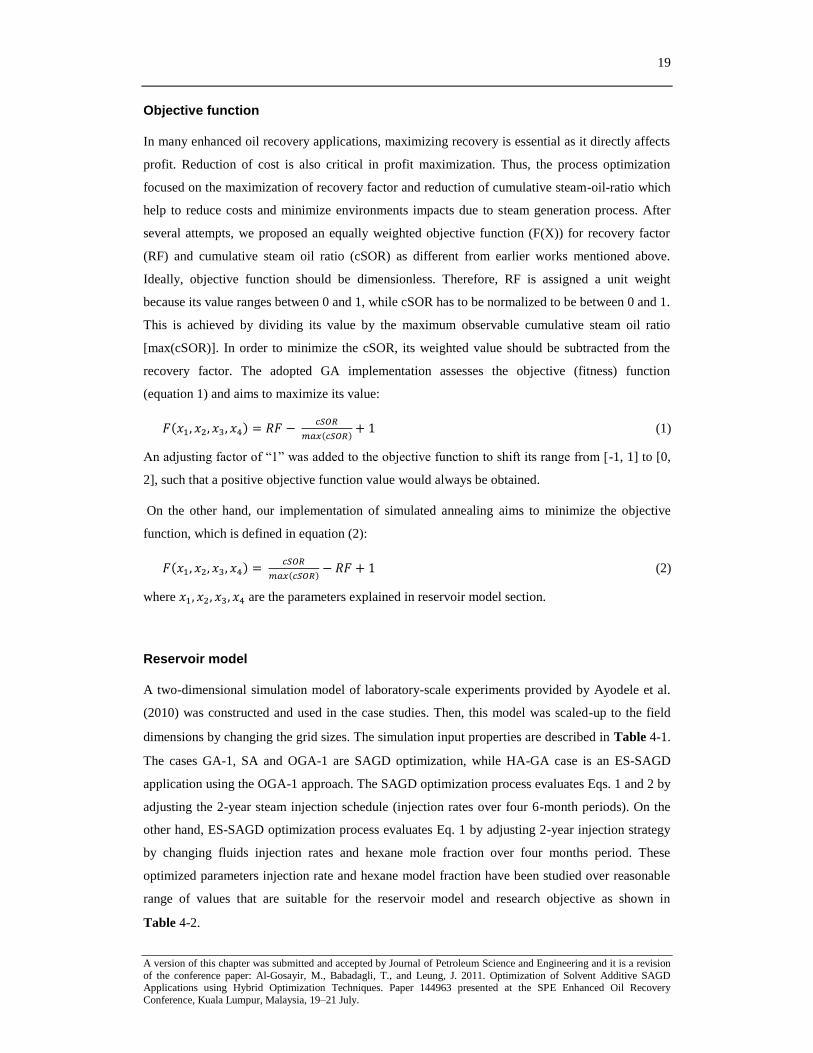
Objective function
In many enhanced oil recovery applications, maximizing recovery is essential as it directly affects
profit. Reduction of cost is also critical in profit maximization. Thus, the process optimization
focused on the maximization of recovery factor and reduction of cumulative steam-oil-ratio which
help to reduce costs and minimize environments impacts due to steam generation process. After
several attempts, we proposed an equally weighted objective function (F(X)) for recovery factor
(RF) and cumulative steam oil ratio (cSOR) as different from earlier works mentioned above.
Ideally, objective function should be dimensionless. Therefore, RF is assigned a unit weight
because its value ranges between 0 and 1, while cSOR has to be normalized to be between 0 and 1.
This is achieved by dividing its value by the maximum observable cumulative steam oil ratio
[max(cSOR)]. In order to minimize the cSOR, its weighted value should be subtracted from the
recovery factor. The adopted GA implementation assesses the objective (fitness) function
(equation 1) and aims to maximize its value:
(1)
Anadjustingfactorof“1”wasaddedtotheobjectivefunctiontoshiftitsrangefrom[-1, 1] to [0,
2], such that a positive objective function value would always be obtained.
On the other hand, our implementation of simulated annealing aims to minimize the objective
function, which is defined in equation (2):
(2)
where are the parameters explained in reservoir model section.
Reservoir model
A two-dimensional simulation model of laboratory-scale experiments provided by Ayodele et al.
(2010) was constructed and used in the case studies. Then, this model was scaled-up to the field
dimensions by changing the grid sizes. The simulation input properties are described in Table 4-1.
The cases GA-1, SA and OGA-1 are SAGD optimization, while HA-GA case is an ES-SAGD
application using the OGA-1 approach. The SAGD optimization process evaluates Eqs. 1 and 2 by
adjusting the 2-year steam injection schedule (injection rates over four 6-month periods). On the
other hand, ES-SAGD optimization process evaluates Eq. 1 by adjusting 2-year injection strategy
by changing fluids injection rates and hexane mole fraction over four months period. These
optimized parameters injection rate and hexane model fraction have been studied over reasonable
range of values that are suitable for the reservoir model and research objective as shown in
Table 4-2.
20
A version of this chapter was submitted and accepted by Journal of Petroleum Science and Engineering and it is a revision
of the conference paper: Al-Gosayir, M., Babadagli, T., and Leung, J. 2011. Optimization of Solvent Additive SAGD Applications using Hybrid Optimization Techniques. Paper 144963 presented at the SPE Enhanced Oil Recovery
Conference, Kuala Lumpur, Malaysia, 19–21 July.
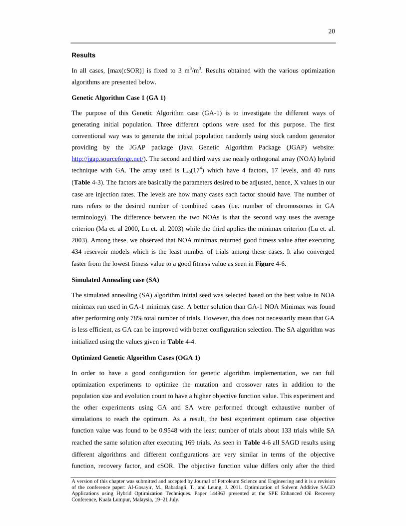
Results
In all cases, [max(cSOR)] is fixed to 3 m3/m
3. Results obtained with the various optimization
algorithms are presented below.
Genetic Algorithm Case 1 (GA 1)
The purpose of this Genetic Algorithm case (GA-1) is to investigate the different ways of
generating initial population. Three different options were used for this purpose. The first
conventional way was to generate the initial population randomly using stock random generator
providing by the JGAP package (Java Genetic Algorithm Package (JGAP) website:
http://jgap.sourceforge.net/). The second and third ways use nearly orthogonal array (NOA) hybrid
technique with GA. The array used is L40(174) which have 4 factors, 17 levels, and 40 runs
(Table 4-3). The factors are basically the parameters desired to be adjusted, hence, X values in our
case are injection rates. The levels are how many cases each factor should have. The number of
runs refers to the desired number of combined cases (i.e. number of chromosomes in GA
terminology). The difference between the two NOAs is that the second way uses the average
criterion (Ma et. al 2000, Lu et. al. 2003) while the third applies the minimax criterion (Lu et. al.
2003). Among these, we observed that NOA minimax returned good fitness value after executing
434 reservoir models which is the least number of trials among these cases. It also converged
faster from the lowest fitness value to a good fitness value as seen in Figure 4-6.
Simulated Annealing case (SA)
The simulated annealing (SA) algorithm initial seed was selected based on the best value in NOA
minimax run used in GA-1 minimax case. A better solution than GA-1 NOA Minimax was found
after performing only 78% total number of trials. However, this does not necessarily mean that GA
is less efficient, as GA can be improved with better configuration selection. The SA algorithm was
initialized using the values given in Table 4-4.
Optimized Genetic Algorithm Cases (OGA 1)
In order to have a good configuration for genetic algorithm implementation, we ran full
optimization experiments to optimize the mutation and crossover rates in addition to the
population size and evolution count to have a higher objective function value. This experiment and
the other experiments using GA and SA were performed through exhaustive number of
simulations to reach the optimum. As a result, the best experiment optimum case objective
function value was found to be 0.9548 with the least number of trials about 133 trials while SA
reached the same solution after executing 169 trials. As seen in Table 4-6 all SAGD results using
different algorithms and different configurations are very similar in terms of the objective
function, recovery factor, and cSOR. The objective function value differs only after the third
21
A version of this chapter was submitted and accepted by Journal of Petroleum Science and Engineering and it is a revision
of the conference paper: Al-Gosayir, M., Babadagli, T., and Leung, J. 2011. Optimization of Solvent Additive SAGD Applications using Hybrid Optimization Techniques. Paper 144963 presented at the SPE Enhanced Oil Recovery
Conference, Kuala Lumpur, Malaysia, 19–21 July.
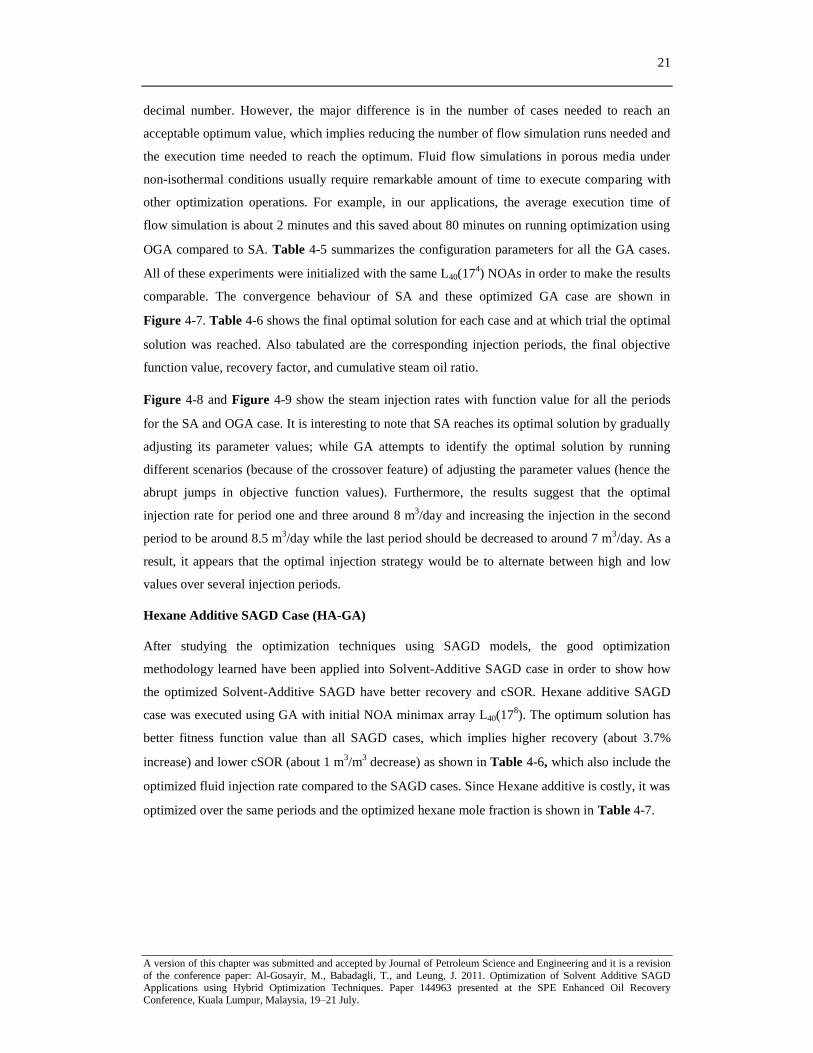
decimal number. However, the major difference is in the number of cases needed to reach an
acceptable optimum value, which implies reducing the number of flow simulation runs needed and
the execution time needed to reach the optimum. Fluid flow simulations in porous media under
non-isothermal conditions usually require remarkable amount of time to execute comparing with
other optimization operations. For example, in our applications, the average execution time of
flow simulation is about 2 minutes and this saved about 80 minutes on running optimization using
OGA compared to SA. Table 4-5 summarizes the configuration parameters for all the GA cases.
All of these experiments were initialized with the same L40(174) NOAs in order to make the results
comparable. The convergence behaviour of SA and these optimized GA case are shown in
Figure 4-7. Table 4-6 shows the final optimal solution for each case and at which trial the optimal
solution was reached. Also tabulated are the corresponding injection periods, the final objective
function value, recovery factor, and cumulative steam oil ratio.
Figure 4-8 and Figure 4-9 show the steam injection rates with function value for all the periods
for the SA and OGA case. It is interesting to note that SA reaches its optimal solution by gradually
adjusting its parameter values; while GA attempts to identify the optimal solution by running
different scenarios (because of the crossover feature) of adjusting the parameter values (hence the
abrupt jumps in objective function values). Furthermore, the results suggest that the optimal
injection rate for period one and three around 8 m3/day and increasing the injection in the second
period to be around 8.5 m3/day while the last period should be decreased to around 7 m
3/day. As a
result, it appears that the optimal injection strategy would be to alternate between high and low
values over several injection periods.
Hexane Additive SAGD Case (HA-GA)
After studying the optimization techniques using SAGD models, the good optimization
methodology learned have been applied into Solvent-Additive SAGD case in order to show how
the optimized Solvent-Additive SAGD have better recovery and cSOR. Hexane additive SAGD
case was executed using GA with initial NOA minimax array L40(178). The optimum solution has
better fitness function value than all SAGD cases, which implies higher recovery (about 3.7%
increase) and lower cSOR (about 1 m3/m
3 decrease) as shown in Table 4-6, which also include the
optimized fluid injection rate compared to the SAGD cases. Since Hexane additive is costly, it was
optimized over the same periods and the optimized hexane mole fraction is shown in Table 4-7.
22
A version of this chapter was submitted and accepted by Journal of Petroleum Science and Engineering and it is a revision
of the conference paper: Al-Gosayir, M., Babadagli, T., and Leung, J. 2011. Optimization of Solvent Additive SAGD Applications using Hybrid Optimization Techniques. Paper 144963 presented at the SPE Enhanced Oil Recovery
Conference, Kuala Lumpur, Malaysia, 19–21 July.
Conclusions
The GA and SA techniques are powerful in finding an optimized solution; however, both require
evaluating number of trials in order to reach the optimum solution which is in our case running
simulation model. Execution of several models requires more computation time.
In this chapter, several optimization techniques were tested to reduce the computational time such
as choosing the right configuration and the initial population or seed. As a result, the SA
converged faster than most of the GA cases. After optimizing the GA configuration, we obtained a
case that converges in reasonable time. Even though the SA converged faster, the GA has some
advantages such as having initial population, which can guide the algorithm to better solution, and
the final population gives more than one scenario that can be used.
On the other hand, the SA may end up being slower than GA if it is initialized with a very bad
seed. In order to improve its performance, several other options can be implemented such as
running the algorithm in parallel computing environment for one flow simulation or running
multiple flow simulations simultaneously, which can be implemented in Genetic Algorithm.
As seen, several options can be used to improve the performance. However, one has to answer the
critical question eventually: what is the most time consuming part? Clearly, the answer is running
time of the flow simulation. Reducing the number of runs by up to 40% is an optimal solution but
it is difficult to obtain such percentage often times as it is hard to know in advance what the best
configuration is. Hence, to reduce the time required for running a flow simulation, implementation
of a proxy, which approximates the flow simulation result in fraction of second instead of two
minutes in our cases, could be a solution. This implies that more than 95% of simulation run time
is saved and all we need is to run a couple of cases to build the proxy.

23
A version of this chapter was submitted and accepted by Journal of Petroleum Science and Engineering and it is a revision
of the conference paper: Al-Gosayir, M., Babadagli, T., and Leung, J. 2011. Optimization of Solvent Additive SAGD Applications using Hybrid Optimization Techniques. Paper 144963 presented at the SPE Enhanced Oil Recovery
Conference, Kuala Lumpur, Malaysia, 19–21 July.
Nomenclature
ANN: Artificial Neural Networks.
cEOR: cumulative net energy-to-oil ratio.
CMG: Computer Modeling Group.
cSOR: steam-to-oil ratio.
F(X): objective function.
GA-1: Genetic Algorithm SAGD cases.
GA: Genetic Algorithm
HA-GA: Hexane Additive SAGD Case executed using GA.
JGAP: Java Genetic Algorithm Package.
NOA: Nearly-Orthogonal Array.
NPV: Net Present Value.
OA: Orthogonal Array.
OGA-1: Optimized Genetic Algorithm configuration SAGD case.
P1, 2, 3, 4: four 6 months injection periods.
RF: Recovery Factor.
SA: Simulated Annealing Algorithm
SAGD: Steam Assisted Gravity Drainage thermal recovery process.
STARS: CMG thermal reservoir simulator.
WAG: Water-Alternating-Gas recovery process.
24
A version of this chapter was submitted and accepted by Journal of Petroleum Science and Engineering and it is a revision
of the conference paper: Al-Gosayir, M., Babadagli, T., and Leung, J. 2011. Optimization of Solvent Additive SAGD Applications using Hybrid Optimization Techniques. Paper 144963 presented at the SPE Enhanced Oil Recovery
Conference, Kuala Lumpur, Malaysia, 19–21 July.
References
Al-Bahlani, A.M. and Babadagli, T. 2009. SAGD Laboratory Experimental and Numerical Simulation
Studies: A Review of Current Status and Future Issues. J. Petr. Sci. and Eng., 68(3-4): 135-150.
Algosayir, M., Leung, J., and Babadagli, T. 2011. Design of Solvent-Assisted SAGD Processes in
Heterogeneous Reservoirs Using Hybrid Optimization Techniques. Paper 149010 presented at the
Canadian Unconventional Resources Conference, Calgary, Alberta, Canada, 15–17 November. DOI:
10.2118/149010-MS
Ayodele, O. R., Nasr, T. N., Ivory, J., Beaulieu, G. and Heck, G. 2010. Testing and History Matching of ES-
SAGD (Using Hexane). Paper 134002 presented at the SPE Western Regional Meeting, Anaheim,
California, USA, 27-29 May. DOI: 10.2118/134002-MS.
Bittencourt, A.C. and Horne, R.N. 1997. Reservoir Development and Design Optimization. Paper 38895
presented at the SPE Annual Technical Conference and Exhibition, San Antonio, Texas, 5-8 October.
DOI: 10.2118/38895-MS.
Chen, S., Li, H., Yang, D., and Tontiwachwuthikul, P. 2010. Optimal Parametric Design for Water-
Alternating-Gas (WAG) Process in a CO2-Miscible Flooding Reservoir. Journal of Canadian Petroleum
Technology 49 (10): 75-82. DOI: 10.2118/141650-PA
ComputerModelingGroup(CMG)Ltd.STARSUser’sManual,Version2009.10.Calgary,Alberta,Canada.
Edmunds N., Moini B., and Peterson J. 2010. Advanced Solvent-Additive Processes by Genetic
Optimization. Journal of Canadian Petroleum Technology 49 (9): 34-41. DOI: 10.2118/140659-PA.
Gates, I.D. and Chakrabarty, N. 2006. Optimization of Steam Assisted Gravity Drainage in McMurray
Reservoir. Journal of Canadian Petroleum Technology 45 (9): 55-62. DOI: 10.2118/06-09-05.
Gates, I.D. and Chakrabarty, N.. 2008. Design of the Steam and Solvent Injection Strategy in Expanding
Solvent Steam-Assisted Gravity Drainage. Journal of Canadian Petroleum Technology 47 (9): 12-20.
DOI: 10.2118/08-09-12-CS.
Guyaguler, B., Horne, R.N., Rogers, L., and Rosenzweig, J.J. 2002. Optimization of Well Placement in a
Gulf of Mexico Waterflooding Project. SPE Reservoir Evaluation & Engineering 5 (3): 229-236. DOI:
10.2118/78266-PA.
Lu, X., Hu, W., and Zheng, Y. 2003. A systematical procedure in the construction of multi-level
supersaturated designs. J. of Statistical Planning & Inference 115 (1): 287-310. DOI: 10.1016/S0378-
3758(02)00116-7.
Ma, C-X., Fang, K-T., and Liski, E. 2000. A new approach in constructing orthogonal and nearly orthogonal
arrays. Metrika 50: 255-268.
Metropolis, N., Rosenbluth, A., Rosenbluth, M., Teller, A., and Teller, E., 1953. Equation of State
Calculations by Fast Computing Machines; Journal of Chemical Physics 21: 1087-1092, June.
DOI:10.1063/1.1699114.
Myers, R.H. and Montgomery D.C. 2002. Response Surface Methodology: Process and Product in
Optimization using Designed Experiments, Wily, New York.
Palke, M.R. and Horne, R.N. 1997. Determining the Value of Reservoir Data by Using Nonlinear Production
Optimization Techniques. Paper SPE 38047 presented at the SPE Asia Pacific Oil and Gas Conference
and Exhibition, Kuala Lumpur, Malaysia, 14-16 April. DOI: 10.2118/38047-MS.

25
A version of this chapter was submitted and accepted by Journal of Petroleum Science and Engineering and it is a revision
of the conference paper: Al-Gosayir, M., Babadagli, T., and Leung, J. 2011. Optimization of Solvent Additive SAGD Applications using Hybrid Optimization Techniques. Paper 144963 presented at the SPE Enhanced Oil Recovery
Conference, Kuala Lumpur, Malaysia, 19–21 July.
Peterson, J., Riva, D., Edmunds, N., and Solanki, S. 2010. The Application of Solvent-Additive SAGD
Processes in Reservoirs With Associated Basal Water. Paper SPE 137833 presented at Canadian
Unconventional Resources and International Petroleum Conference, Calgary, Alberta, Canada, 19-21
October. DOI: 10.2118/137833-MS.
26
A version of this chapter was submitted and accepted by Journal of Petroleum Science and Engineering and it is a revision
of the conference paper: Al-Gosayir, M., Babadagli, T., and Leung, J. 2011. Optimization of Solvent Additive SAGD Applications using Hybrid Optimization Techniques. Paper 144963 presented at the SPE Enhanced Oil Recovery
Conference, Kuala Lumpur, Malaysia, 19–21 July.
Tables
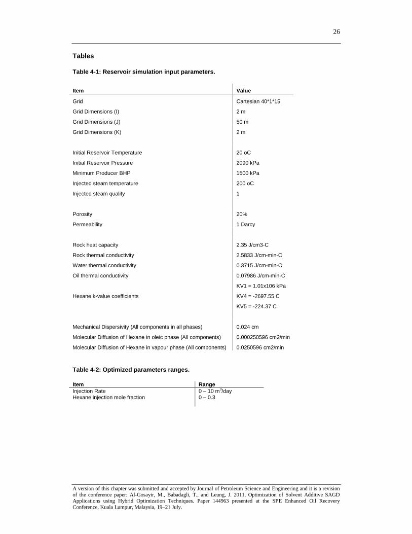
Table 4-1: Reservoir simulation input parameters.
Item Value
Grid Cartesian 40*1*15
Grid Dimensions (I) 2 m
Grid Dimensions (J) 50 m
Grid Dimensions (K) 2 m
Initial Reservoir Temperature 20 oC
Initial Reservoir Pressure 2090 kPa
Minimum Producer BHP 1500 kPa
Injected steam temperature 200 oC
Injected steam quality 1
Porosity 20%
Permeability 1 Darcy
Rock heat capacity 2.35 J/cm3-C
Rock thermal conductivity 2.5833 J/cm-min-C
Water thermal conductivity 0.3715 J/cm-min-C
Oil thermal conductivity 0.07986 J/cm-min-C
Hexane k-value coefficients
KV1 = 1.01x10⁶ kPa
KV4 = -2697.55 C
KV5 = -224.37 C
Mechanical Dispersivity (All components in all phases) 0.024 cm
Molecular Diffusion of Hexane in oleic phase (All components) 0.000250596 cm2/min
Molecular Diffusion of Hexane in vapour phase (All components) 0.0250596 cm2/min
Table 4-2: Optimized parameters ranges.
Item Range
Injection Rate 0 – 10 m3/day
Hexane injection mole fraction 0 – 0.3

27
A version of this chapter was submitted and accepted by Journal of Petroleum Science and Engineering and it is a revision
of the conference paper: Al-Gosayir, M., Babadagli, T., and Leung, J. 2011. Optimization of Solvent Additive SAGD Applications using Hybrid Optimization Techniques. Paper 144963 presented at the SPE Enhanced Oil Recovery
Conference, Kuala Lumpur, Malaysia, 19–21 July.
Table 4-3: NOA Tables.
Average Criterion Array
Minimax Criterion Array
Factors
Factors
Run 1 2 3 4
Run 1 2 3 4
1 3 7 7 9
1 9 9 0 0
2 3 8 5 8
2 8 2 3 3
3 9 9 1 0
3 6 5 6 4
4 4 2 5 4
4 8 4 6 9
5 1 4 1 1
5 1 8 0 10
6 2 0 4 6
6 0 2 5 8
7 6 0 1 2
7 4 3 8 4
8 3 5 3 8
8 6 3 9 2
9 9 1 3 8
9 9 3 3 7
10 1 10 3 7
10 1 3 1 3
11 4 3 6 9
11 4 5 8 3
12 0 9 9 10
12 5 1 8 7
13 10 5 8 3
13 1 9 1 9
14 5 1 4 1
14 0 6 1 1
15 0 6 3 2
15 1 7 8 2
16 7 6 1 4
16 6 9 3 0
17 1 1 9 5
17 3 0 9 4
18 9 3 8 0
18 7 2 9 3
19 8 1 6 8
19 3 0 4 8
20 8 4 3 4
20 2 9 6 1
21 4 10 9 3
21 0 4 7 6
22 7 2 1 1
22 4 10 2 5
23 2 6 6 1
23 4 1 10 9
24 3 1 9 0
24 3 4 1 6
25 3 3 10 6
25 5 6 3 3
26 2 4 4 3
26 8 1 10 10
27 1 8 2 3
27 1 3 6 1
28 10 3 2 4
28 3 4 0 8
29 5 4 2 1
29 3 6 4 3
30 4 3 3 9
30 9 1 2 9
31 6 6 10 6
31 10 0 5 0
32 6 9 0 9
32 3 8 3 1
33 1 0 6 7
33 2 8 9 5
34 9 8 7 3
34 10 6 3 6
35 0 3 8 1
35 6 10 4 1
36 6 7 0 3
36 2 3 1 2
37 3 2 0 2
37 9 8 4 8
38 1 8 8 6
38 8 1 2 6
39 8 1 1 10
39 7 7 1 1
40 8 9 4 5
40 1 1 7 4
Table 4-4: Simulated annealing configuration.
Initial temperature 1
Acceptance rule temperature 1
Maximum temperature iterations 600
Random moves 10
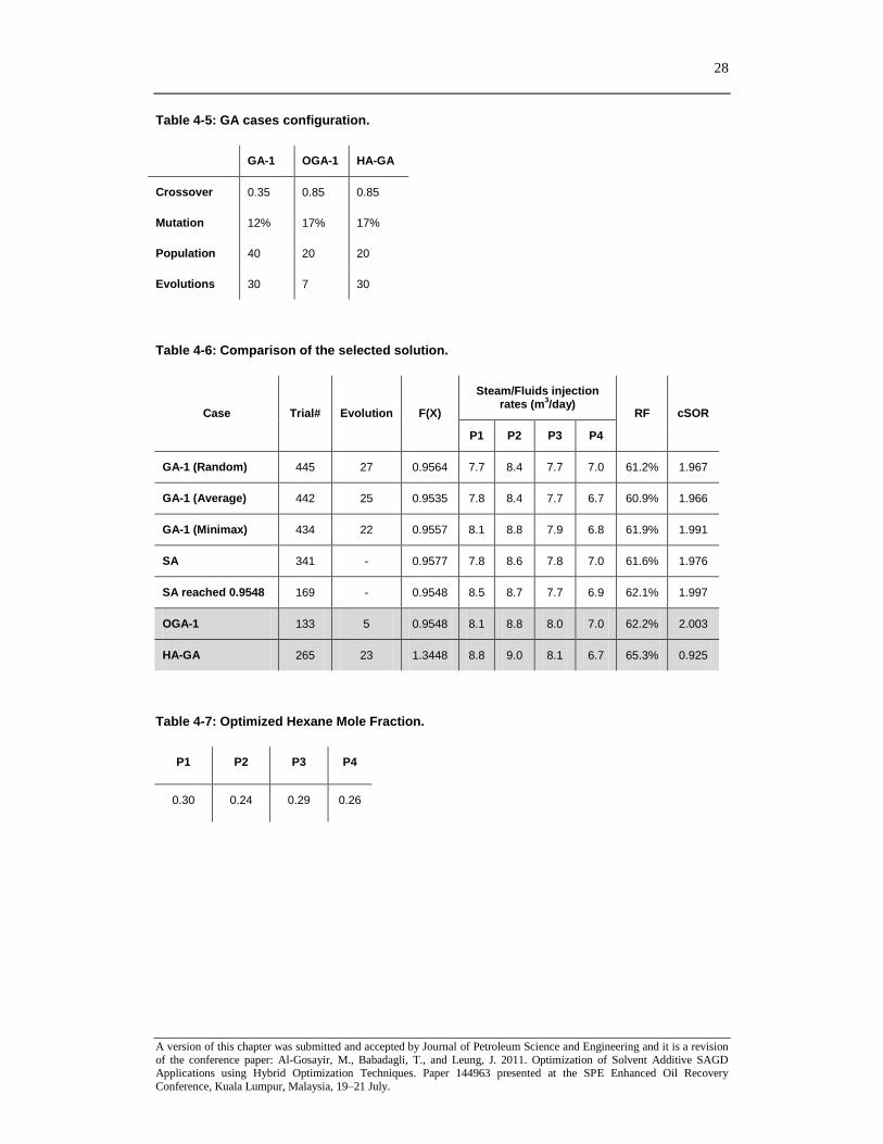
28
A version of this chapter was submitted and accepted by Journal of Petroleum Science and Engineering and it is a revision
of the conference paper: Al-Gosayir, M., Babadagli, T., and Leung, J. 2011. Optimization of Solvent Additive SAGD Applications using Hybrid Optimization Techniques. Paper 144963 presented at the SPE Enhanced Oil Recovery
Conference, Kuala Lumpur, Malaysia, 19–21 July.
Table 4-5: GA cases configuration.
GA-1 OGA-1 HA-GA
Crossover 0.35 0.85 0.85
Mutation 12% 17% 17%
Population 40 20 20
Evolutions 30 7 30
Table 4-6: Comparison of the selected solution.
Case Trial# Evolution F(X)
Steam/Fluids injection rates (m
3/day)
RF cSOR
P1 P2 P3 P4
GA-1 (Random) 445 27 0.9564 7.7 8.4 7.7 7.0 61.2% 1.967
GA-1 (Average) 442 25 0.9535 7.8 8.4 7.7 6.7 60.9% 1.966
GA-1 (Minimax) 434 22 0.9557 8.1 8.8 7.9 6.8 61.9% 1.991
SA 341 - 0.9577 7.8 8.6 7.8 7.0 61.6% 1.976
SA reached 0.9548 169 - 0.9548 8.5 8.7 7.7 6.9 62.1% 1.997
OGA-1 133 5 0.9548 8.1 8.8 8.0 7.0 62.2% 2.003
HA-GA 265 23 1.3448 8.8 9.0 8.1 6.7 65.3% 0.925
Table 4-7: Optimized Hexane Mole Fraction.
P1 P2 P3 P4
0.30 0.24 0.29 0.26
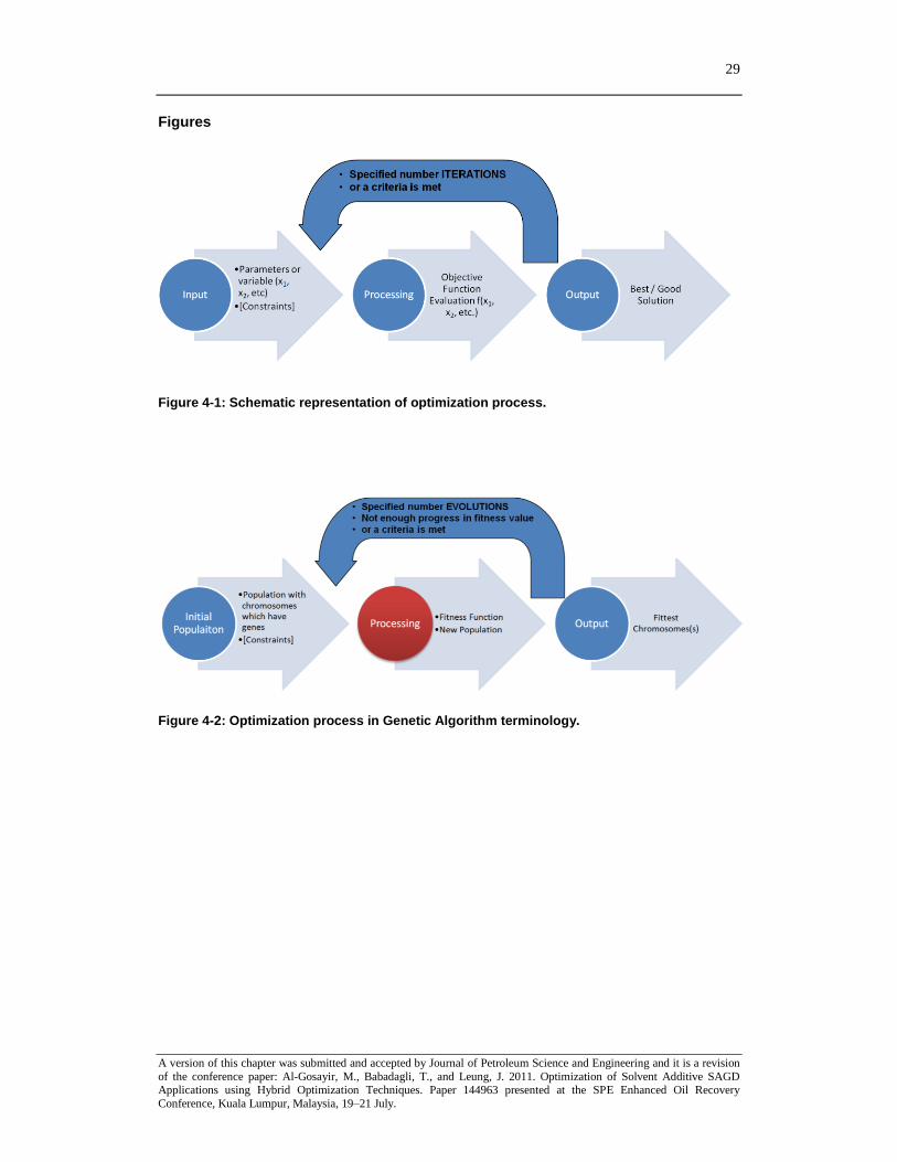
29
A version of this chapter was submitted and accepted by Journal of Petroleum Science and Engineering and it is a revision
of the conference paper: Al-Gosayir, M., Babadagli, T., and Leung, J. 2011. Optimization of Solvent Additive SAGD Applications using Hybrid Optimization Techniques. Paper 144963 presented at the SPE Enhanced Oil Recovery
Conference, Kuala Lumpur, Malaysia, 19–21 July.
Figures
Figure 4-1: Schematic representation of optimization process.
Figure 4-2: Optimization process in Genetic Algorithm terminology.
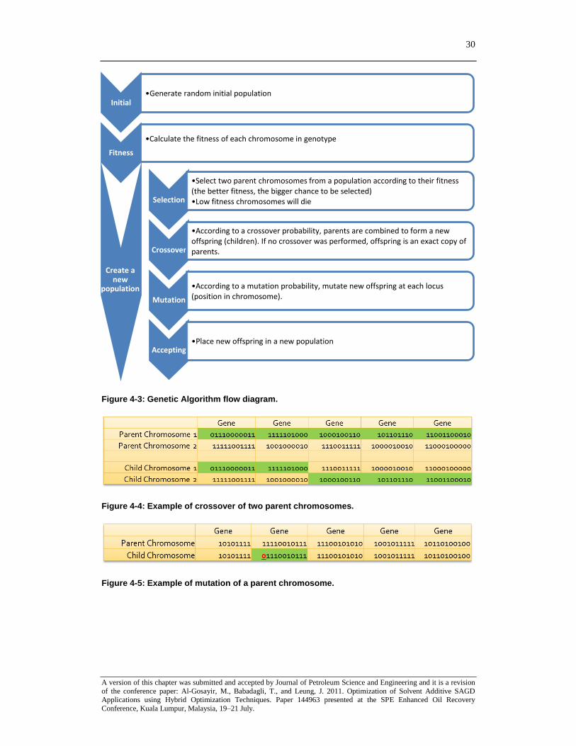
30
A version of this chapter was submitted and accepted by Journal of Petroleum Science and Engineering and it is a revision
of the conference paper: Al-Gosayir, M., Babadagli, T., and Leung, J. 2011. Optimization of Solvent Additive SAGD Applications using Hybrid Optimization Techniques. Paper 144963 presented at the SPE Enhanced Oil Recovery
Conference, Kuala Lumpur, Malaysia, 19–21 July.
Figure 4-3: Genetic Algorithm flow diagram.
Figure 4-4: Example of crossover of two parent chromosomes.
Figure 4-5: Example of mutation of a parent chromosome.
Initial •Generate random initial population
Fitness
•Calculate the fitness of each chromosome in genotype
Selection
•Select two parent chromosomes from a population according to their fitness (the better fitness, the bigger chance to be selected) •Low fitness chromosomes will die
Crossover
•According to a crossover probability, parents are combined to form a new offspring (children). If no crossover was performed, offspring is an exact copy of parents.
Mutation
•According to a mutation probability, mutate new offspring at each locus (position in chromosome).
Accepting •Place new offspring in a new population
Create a new
population
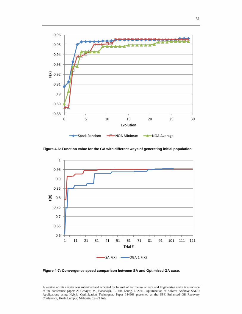
31
A version of this chapter was submitted and accepted by Journal of Petroleum Science and Engineering and it is a revision
of the conference paper: Al-Gosayir, M., Babadagli, T., and Leung, J. 2011. Optimization of Solvent Additive SAGD Applications using Hybrid Optimization Techniques. Paper 144963 presented at the SPE Enhanced Oil Recovery
Conference, Kuala Lumpur, Malaysia, 19–21 July.
Figure 4-6: Function value for the GA with different ways of generating initial population.
Figure 4-7: Convergence speed comparison between SA and Optimized GA case.
0.88
0.89
0.9
0.91
0.92
0.93
0.94
0.95
0.96
0 5 10 15 20 25 30
F(X
)
Evolution
Stock Random NOA Minimax NOA Average
0.6
0.65
0.7
0.75
0.8
0.85
0.9
0.95
1
1 11 21 31 41 51 61 71 81 91 101 111 121
F(X
)
Trial #
SA F(X) OGA 1 F(X)
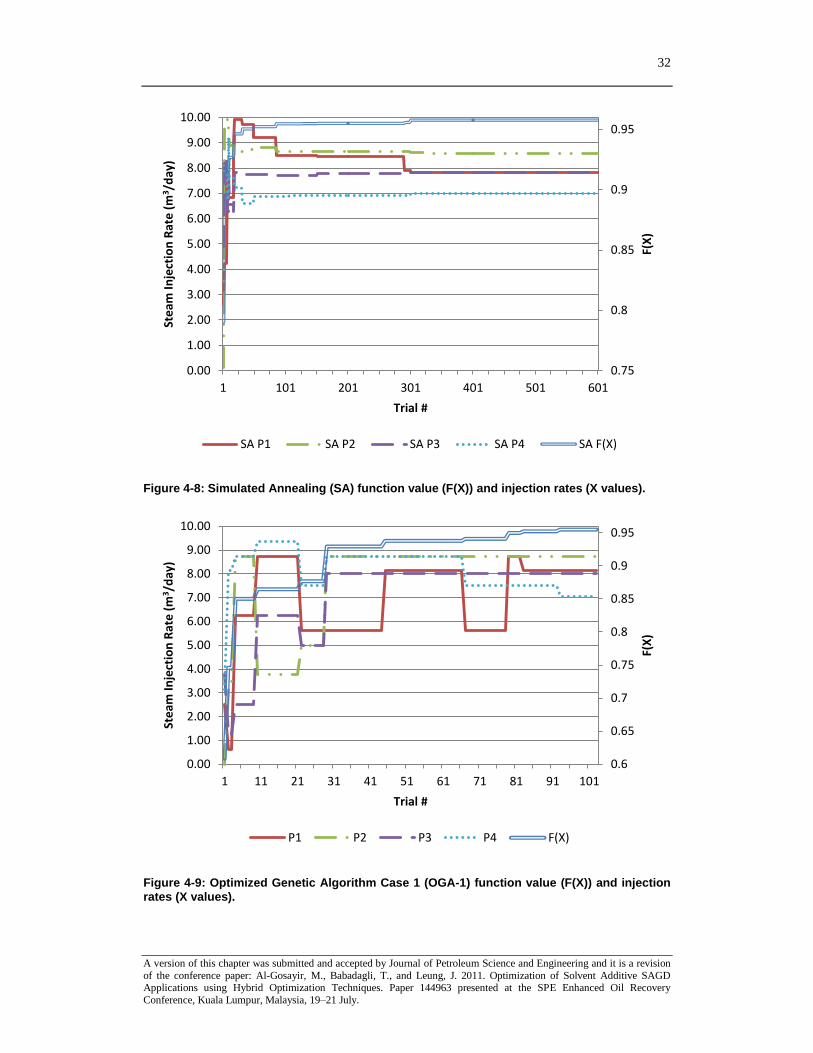
32
A version of this chapter was submitted and accepted by Journal of Petroleum Science and Engineering and it is a revision
of the conference paper: Al-Gosayir, M., Babadagli, T., and Leung, J. 2011. Optimization of Solvent Additive SAGD Applications using Hybrid Optimization Techniques. Paper 144963 presented at the SPE Enhanced Oil Recovery
Conference, Kuala Lumpur, Malaysia, 19–21 July.
Figure 4-8: Simulated Annealing (SA) function value (F(X)) and injection rates (X values).
Figure 4-9: Optimized Genetic Algorithm Case 1 (OGA-1) function value (F(X)) and injection
rates (X values).
0.75
0.8
0.85
0.9
0.95
0.00
1.00
2.00
3.00
4.00
5.00
6.00
7.00
8.00
9.00
10.00
1 101 201 301 401 501 601
F(X
)
Ste
am In
ject
ion
Rat
e (
m3/d
ay)
Trial #
SA P1 SA P2 SA P3 SA P4 SA F(X)
0.6
0.65
0.7
0.75
0.8
0.85
0.9
0.95
0.00
1.00
2.00
3.00
4.00
5.00
6.00
7.00
8.00
9.00
10.00
1 11 21 31 41 51 61 71 81 91 101
F(X
)
Ste
am In
ject
ion
Rat
e (
m3/d
ay)
Trial #
P1 P2 P3 P4 F(X)
33
A version of this chapter was submitted and accepted by Journal of Canadian Petroleum Technology and it is a revision of
the conference paper: Al-Gosayir, M., Leung, J., and Babadagli, T., 2011b. Design of Solvent-Assisted SAGD Processes in Heterogeneous Reservoirs Using Hybrid Optimization Techniques. Paper 149010 presented at the Canadian
Unconventional Resources Conference, Calgary, Canada, 15–17 November. DOI: 10.2118/149010-MS.
Chapter 5: Design of Solvent-Assisted SAGD Processes in Heterogeneous Reservoirs Using
Hybrid Optimization Techniques
Abstract
Many Steam Assisted Gravity Drainage (SAGD) optimization studies published in the literature
combined numerical simulation with graphical or analytical techniques for design and
performance evaluation. There have been numerous efforts that integrated the simulation exercise
with global optimization algorithms. Some studies focused on optimization of cumulative steam-
to-oil ratio (cSOR) in SAGD by altering steam injection rates, while others focused on
optimization of cumulative net energy-to-oil ratio (cEOR) in solvent-additive SAGD by altering
injection pressures and fraction of solvent in the injection stream. Several studies also considered
total project net present value calculation by changing total project area, capital cost intensities,
solvent prices, and risk factors to determine the well spacing and drilling schedule. Optimization
techniques commonly used in those studies were scattered search, simulated annealing, and
genetic algorithm (GA). However, the applications of hybrid genetic algorithm were rarely found.
In this chapter, we focused on optimization of solvent-assisted SAGD using various GA
implementations. In our models, hexane was selected to be co-injected with steam. The objective
function, defined based on cumulative steam-oil ratio (cSOR) and recovery factor, was optimized
by changing injection pressures, production pressures, and injected solvent-to-steam ratio.
Techniquesincludingorthogonalarrays(OA)forexperimentaldesign(e.g.Taguchi’sarrays)and
proxy models for objective function evaluations were incorporated with the GA method to
improve computational and convergence efficiency. Results from these hybrid approaches
revealed that an optimized solution could be achieved with less CPU time (e.g. fewer number of
iterations) compared to the conventional GA method. Sensitivity analysis was also conducted on
the choice of proxy model to study the robustness of the proposed methods.
To investigate the effects of heterogeneity in the design process, optimization of solvent-assisted
SAGD was performed on various synthetic heterogeneous reservoir models of porosity,
permeability, and shale distributions. Our results highlight the potential application of the
proposed techniques in other solvent-enhanced heavy oil recovery processes.
34
A version of this chapter was submitted and accepted by Journal of Canadian Petroleum Technology and it is a revision of
the conference paper: Al-Gosayir, M., Leung, J., and Babadagli, T., 2011b. Design of Solvent-Assisted SAGD Processes in Heterogeneous Reservoirs Using Hybrid Optimization Techniques. Paper 149010 presented at the Canadian
Unconventional Resources Conference, Calgary, Canada, 15–17 November. DOI: 10.2118/149010-MS.
Introduction
Different versions of steam injection areused toextractmostofAlberta’soilsandreserves(Al-
Bahlani and Babadagli, 2009). The most common application is Steam Assisted Gravity Drainage
(SAGD) recovery. It, however, requires generation of excessive amount of steam, which is very
costly and has adverse environmental impacts, and it is often considered as a limiting factor in the
efficiency of the entire process. One of the suggested ways to reduce steam consumption is
addition of solvent to steam to maximize the recovery.
Several studies focused on optimization of SAGD processes that are with or without solvent
addition. A number of efforts focused on utilizing global optimization techniques. Gates and
Chakrabarty (2006) used genetic algorithm in order to optimize SAGD operating conditions such
as steam injection rates to reduce cumulative steam-to-oil ratio (cSOR). The same authors have
also implemented simulated annealing to optimize expanded solvent SAGD (ES-SAGD) by
altering the fraction of solvent in the injected steam and the injection pressures in order to reduce
cumulative net energy-to-oil ratio (cEOR) (Gates and Chakrabarty, 2008). Yang et al. (2009)
applied the Designed Exploration and Controlled Evolution (DECE) algorithm to optimize the net
present value (NPV) of a three-dimensional model. Peterson et al. (2010) utilized genetic
algorithm to optimize steam and solvent rates on solvent-additive SAGD to maximize NPV per
hectare of land (NPV/ha).
Having an efficient and robust optimization technique is critical in the design of SAGD or solvent-
additive SAGD processes. Hence, this work focuses on hybrid techniques to enhance the
computational efficiency of the Genetic Algorithm to design solvent-additive SAGD processes in
heterogeneous reservoirs.
Methodology
Global Optimization Techniques
In this chapter, we adopted the Genetic Algorithm (GA) and integrated it with two other
techniques in a hybrid formulation. GA is a stochastic search technique based on the principle of
“survival of the fittest” (Guyaguler et al., 2002; Chen et al., 2010). An initial population or
genotype is constructed by sampling the solution space randomly. Individual members of the
population are called “chromosomes”, and they define the parameter sets for the optimization
problem. In each evolution, the fitness of each chromosome is calculated. Then, multiple pairs are
selected based on their fitness value to create an offspring via crossover and mutation. The new
offspring is inserted in the population, while the chromosomes with lowest fitness values are
discarded. Figure 5-1 summarizes the mechanisms of a typical GA algorithm.
35
A version of this chapter was submitted and accepted by Journal of Canadian Petroleum Technology and it is a revision of
the conference paper: Al-Gosayir, M., Leung, J., and Babadagli, T., 2011b. Design of Solvent-Assisted SAGD Processes in Heterogeneous Reservoirs Using Hybrid Optimization Techniques. Paper 149010 presented at the Canadian
Unconventional Resources Conference, Calgary, Canada, 15–17 November. DOI: 10.2118/149010-MS.
To improve the convergence behaviour and computational efficiency of GA, we proposed a hybrid
formulation by integrating the following two techniques into the conventional framework of GA:
Orthogonal Array and Nearly-Orthogonal Array for Initial Population Generation
Techniques from the experimental design literature, namely Orthogonal Array (OA) and Nearly-
Orthogonal Array (NOA), can be implemented with GA to improve the quality of initial
population (Chen et al., 2010) by generating evenly distributed samples while reducing the
redundancy between chromosomes. The objective is to design experiments or chromosomes by
determining the levels at which the parameters should be varied. Instead of testing all
combinations of parameters at all levels, only the ones containing principal information are
included. This reduces the population size and the associated computational costs. In this study,
we used Gendex DOE Toolkit (website: http://designcomputing.net/gendex) to generate nearly-
orthogonal arrays based on the Taguchi method average criterion described by Ma et. al. (2000)
and Lu et. al. (2003).
Proxy Method for Objective Function Evaluation
As can be seen in Figure 5-1, the fitness function must be evaluated for every chromosome at
every evolution. In our particular application, evaluation of the fitness function involves
calculation of the recovery factor, typically obtained from results of a numerical flow simulation.
Depending on the level of complexity of the processes that are being modeled, each flow
simulation could take up to days to complete. Hence, costs of objective function evaluation are
often the most important computational considerations in any optimization scheme. Proxy
methodsareviable“cheaper”alternativesthatapproximate the actual fitness function to enhance
computing efficiency. The technique implemented in this study was the response surface method.
Response surface is a relationship between the parameter sets and the corresponding fitness
function. Once calibrated in the form of regression, it can be used as a proxy for flow simulation
and allows the fitness function to be evaluated rapidly. In particular, we compared the first-order
linear model and the second-order non-linear model, as discussed in Myers and Montgomery
(2002). Equations for the linear and non-linear models are shown in Eqs. 1 and 2, respectively,
where J is the response (fitness function value), ui’s are the variables (optimization parameters),
βi’saretheregressioncoefficients,andε is an error term.
(1)
∑
∑ ∑ (2)
The regression equation for both models is expressed in Eq. 3:
(3)
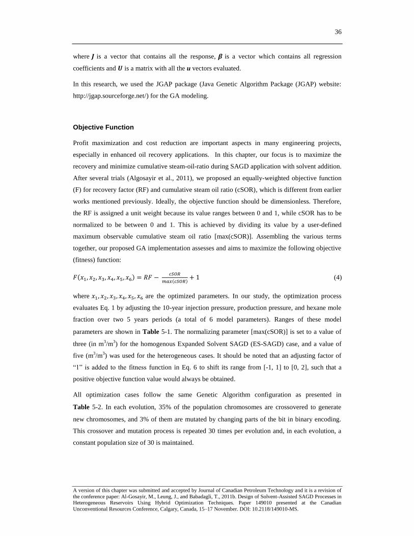
36
A version of this chapter was submitted and accepted by Journal of Canadian Petroleum Technology and it is a revision of
the conference paper: Al-Gosayir, M., Leung, J., and Babadagli, T., 2011b. Design of Solvent-Assisted SAGD Processes in Heterogeneous Reservoirs Using Hybrid Optimization Techniques. Paper 149010 presented at the Canadian
Unconventional Resources Conference, Calgary, Canada, 15–17 November. DOI: 10.2118/149010-MS.
where is a vector that contains all the response, is a vector which contains all regression
coefficients and is a matrix with all the u vectors evaluated.
In this research, we used the JGAP package (Java Genetic Algorithm Package (JGAP) website:
http://jgap.sourceforge.net/) for the GA modeling.
Objective Function
Profit maximization and cost reduction are important aspects in many engineering projects,
especially in enhanced oil recovery applications. In this chapter, our focus is to maximize the
recovery and minimize cumulative steam-oil-ratio during SAGD application with solvent addition.
After several trials (Algosayir et al., 2011), we proposed an equally-weighted objective function
(F) for recovery factor (RF) and cumulative steam oil ratio (cSOR), which is different from earlier
works mentioned previously. Ideally, the objective function should be dimensionless. Therefore,
the RF is assigned a unit weight because its value ranges between 0 and 1, while cSOR has to be
normalized to be between 0 and 1. This is achieved by dividing its value by a user-defined
maximum observable cumulative steam oil ratio [max(cSOR)]. Assembling the various terms
together, our proposed GA implementation assesses and aims to maximize the following objective
(fitness) function:
(4)
where are the optimized parameters. In our study, the optimization process
evaluates Eq. 1 by adjusting the 10-year injection pressure, production pressure, and hexane mole
fraction over two 5 years periods (a total of 6 model parameters). Ranges of these model
parameters are shown in Table 5-1. The normalizing parameter [max(cSOR)] is set to a value of
three (in m3/m
3) for the homogenous Expanded Solvent SAGD (ES-SAGD) case, and a value of
five (m3/m
3) was used for the heterogeneous cases. It should be noted that an adjusting factor of
“1” isadded to the fitness function in Eq. 6 to shift its range from [-1, 1] to [0, 2], such that a
positive objective function value would always be obtained.
All optimization cases follow the same Genetic Algorithm configuration as presented in
Table 5-2. In each evolution, 35% of the population chromosomes are crossovered to generate
new chromosomes, and 3% of them are mutated by changing parts of the bit in binary encoding.
This crossover and mutation process is repeated 30 times per evolution and, in each evolution, a
constant population size of 30 is maintained.
37
A version of this chapter was submitted and accepted by Journal of Canadian Petroleum Technology and it is a revision of
the conference paper: Al-Gosayir, M., Leung, J., and Babadagli, T., 2011b. Design of Solvent-Assisted SAGD Processes in Heterogeneous Reservoirs Using Hybrid Optimization Techniques. Paper 149010 presented at the Canadian
Unconventional Resources Conference, Calgary, Canada, 15–17 November. DOI: 10.2118/149010-MS.
Case Study
Model Description
In our case studies, three two-dimensional simulation models were constructed originally based on
the laboratory-scale simulation model with homogeneous and isotropic reservoir properties
provided by Ayodele et al. (2010). These models were subsequently scaled-up to the field
dimensions by adjusting the grid definition as described in Table 5-3. The homogenous model has
a constant porosity of 20% and permeability of 1 Darcy for all cells. The homogeneous model was
used to (1) investigate the sensitivity of the optimization results to the choice of response surface
proxy models and (2) assess the computational savings with the use of proxy techniques as
compared to the conventional method (no proxy). Success with the homogeneous case allows us to
subsequently apply the proposed implementation to cases with heterogeneous reservoir properties.
In particular, two heterogeneous models exhibiting different shale distributions (30% and 10%
shale content) were used in our study, and they are shown in Figure 5-2 and Figure 5-3,
respectively.
Response Surface Proxy Models
To reduce the computation time required, a linear first-order (Eq. 1) and non-linear second-order
(Eq. 2) response surface models were constructed for the three reservoir models. These proxies (or
response surfaces) were calibrated using flow simulations results of an initial population,
constructed using the nearly-orthogonal array (NOA) L30(176) consists of 6 factors, 17 levels, and
30 runs (Table 5-4) and applying Eqs. 1-3.
Results and Discussion
The primary objective of this chapter is to study the impacts of reservoir heterogeneities on the
optimization of solvent-assisted SAGD recovery process. Given that objective function
evaluations using detailed flow simulation results are extremely time consuming, particularly for
heterogeneous reservoirs, our first step is to evaluate various response surface proxy techniques
that can be easily integrated for GA optimization.
First, we established a base case by performing conventional GA optimization (no proxy) for a
homogenous reservoir with an initial population constructed using the NOA in Table 5-4. The
entire experiment required a total of 52 hours to execute about 900 simulation cases to obtain the
optimum, which has 1.31 fitness value, 68% recovery and 1.13 (m3/m
3) cSOR. Figure 5-4 shows
the oil production profile for the optimum field scale case. In order to evaluate the reproducibility
of our optimization results, we repeated the optimization experiment and similar results were
obtained: 1.32 fitness value, 69% recovery and 1.14 (m3/m
3) cSOR. Results of the two trials are
labelledas“Conventional(1)”and“Conventional(2)”,respectivelyinTable 5-5. Next, linear and
38
A version of this chapter was submitted and accepted by Journal of Canadian Petroleum Technology and it is a revision of
the conference paper: Al-Gosayir, M., Leung, J., and Babadagli, T., 2011b. Design of Solvent-Assisted SAGD Processes in Heterogeneous Reservoirs Using Hybrid Optimization Techniques. Paper 149010 presented at the Canadian
Unconventional Resources Conference, Calgary, Canada, 15–17 November. DOI: 10.2118/149010-MS.
non-linear response surface proxies were tested. The proxies were constructed based on flow
simulation results of the initial population generated using the NOA. In other words, the
computation requirement was reduced significantly to only that was required to execute the cases
of the initial population. It was observed that the non-linear proxy approximated the initial data
actual responses closely while the match with the linear proxy was not satisfactory as shown in
Figure 5-5. The trials are sorted based on the fitness values obtained from actual flow simulations.
Similarly, we built linear and non-linear proxies for the 30% and 10% shale content
(heterogeneous) cases as shown in Figure 5-6 and Figure 5-7, respectively. In the 30% case, the
non-linear shows excellent match, while in the 10% case, it did not yield a satisfactory match.
In the homogenous case, optimization performed with the linear proxy was completely
unsuccessful as it was not able to improve the fitness during the evolutions. On the other hand, the
non-linear proxy showed very good improvement in the fitness function value during the
evolutions as shown in Figure 5-8. In order to compare the optimal solution obtained using the
proxy to that of the conventional approach, we performed flow simulation on the final optimized
solution to obtain the actual response J, instead of the proxy estimated value J’. In the case of
linear proxy, the actual response J was lower than the best case in the initial population J0,
indicating that the fitness function was not maximized. In contrast, for the case of non-linear
proxy, the actual response J matched closely with the conventional optimization result even
though the proxy was amplifying the response values. This is due to the extrapolation of the
response surface corresponding to parts of parameter space. The actual response value for the
optimum case Jopt was 1.3 with 68% recovery and 1.15 (m3/m
3) cSOR as shown in Table 5-5. It is
important to note that this result was obtained in 105 minutes where we saved about 97% of the
computational efforts from the conventional optimization as indicated in Table 5-6.
This improvement in computational efficiency becomes particularly important in applications for
heterogeneous reservoirs because of the increase in flow simulation execution time with reservoir
heterogeneity. On average, a single flow simulation in this study takes about five minutes for the
30% shale case and about 6 minutes for the 10% shale case to execute. If optimization of these
heterogeneous models was performed with the conventional GA implementation, the
computational time would have been over three days, thus rendering the method unfeasible due to
computational constraints. This consideration motivates the use of proxy for objective function
evaluation and allows optimization to be performed efficiently in the case of heterogeneous
reservoirs. Our proposed hybrid approach took 138 minutes for the 30% shale case and 187
minutes for 10% shale case to complete (Table 5-6). This is equivalent to a savings of 152 hours
(or approximately 97%) of the total computational time.
39
A version of this chapter was submitted and accepted by Journal of Canadian Petroleum Technology and it is a revision of
the conference paper: Al-Gosayir, M., Leung, J., and Babadagli, T., 2011b. Design of Solvent-Assisted SAGD Processes in Heterogeneous Reservoirs Using Hybrid Optimization Techniques. Paper 149010 presented at the Canadian
Unconventional Resources Conference, Calgary, Canada, 15–17 November. DOI: 10.2118/149010-MS.
Our results suggest that the performance of the linear proxy in the heterogeneous cases was better
than the homogenous case; the fitness function increased with evolution shown in Figure 5-9 and
Figure 5-10 as opposed to staying constant in Figure 5-8. However, the non-linear proxy was still
providing better results. For the 30% shale case, the linear proxy actual response value for the
optimum case Jopt was 0.65 with 5% recovery and 1.98 (m3/m
3) cSOR while the non-linear proxy
actual response value for the optimum case Jopt was 0.71 with 7% recovery and 1.77 (m3/m
3)
cSOR. Similarly, in the 10% shale case, the linear proxy actual response value for the optimum
case Jopt was 1.13 with 40% recovery and 1.28 (m3/m
3) cSOR while the non-linear proxy actual
response value for the optimum case Jopt was 1.14 with 42% recovery and 1.38 (m3/m
3) cSOR.
Optimization results of all cases are shown in Table 5-5. It is worthwhile to point out that the
calculated response value J’ of the linear proxy is similar in range to the actual value J, while
higher degree of extrapolation in the non-linear proxy model leads to a larger deviation from this
range.
Several ways were investigated to reduce the degree of extrapolation and to obtain more accurate
approximation of the fitness function using the non-linear proxy. The approach that gave the most
promising results was the one where flow simulation was performed for the fittest chromosome
after every evolution, and the corresponding simulation result would be incorporated to fit a new
proxy. It was observed that updating the proxy after evolution with an additional flow simulation
output using the fittest chromosome could significantly improve the predictability of the non-
linear proxy. The flow diagram of the modified approach is shown in Figure 5-11. It is noted from
Figure 5-12 that each time the proxy was updated using the fittest chromosome’s simulation
results, more accurate proxy values (as compared to the actual flow simulation outputs) were
achieved. Figure 5-12 also shows that towards the end of the optimization exercise, there was no
noticeable differences between the proxy values and actual flow simulation outputs, indicating that
the predictability of the non-linear was significantly improved. Finally, as shown in Table 5-5,
applying this modified approach to the homogeneous case achieved a better (more optimized)
scenario than the conventional method with a higher fitness value of 1.4, a higher recovery of 76%
and a lower cSOR of 1.07 (m3/m
3).
The modified approach was also applied to the 10% and 30% shale cases to update the non-linear
proxy after every evolution. Similar improvement as in the homogeneous case was achieved:
updating the proxy using the fittest chromosome after every evolution gave the best optimized
parameters among all scenarios, while the proxy predictability was excellent (as evidenced by the
identicalvaluesforJandJ’ in Table 5-5). The optimization results (fitness value as a function of
evolution) are shown in Figure 5-13 and Figure 5-14. It should be noted that the total number of
flow simulation runs performed in this modified approach was 90 (30 for the initial population
40
A version of this chapter was submitted and accepted by Journal of Canadian Petroleum Technology and it is a revision of
the conference paper: Al-Gosayir, M., Leung, J., and Babadagli, T., 2011b. Design of Solvent-Assisted SAGD Processes in Heterogeneous Reservoirs Using Hybrid Optimization Techniques. Paper 149010 presented at the Canadian
Unconventional Resources Conference, Calgary, Canada, 15–17 November. DOI: 10.2118/149010-MS.
plus an additional one per every evolution). The increased computational expenses could easily be
justified given the considerable improvements in the predictability of the response surface models
and the final optimized scenario. Furthermore, the computational savings as compared to the
conventional approach is still important (Table 5-6).
Conclusions
Proxy methods are convenient ways to improve efficiency of an optimization algorithm. In our
application, we observed that the execution time for objective function evaluation is the largest.
Other factors like the algorithm convergence speed and the input/output (I/O) processing that
serves as an interface between the flow simulator and the rest of the algorithm implementation are
negligible in comparison to the time needed to execute the simulation. This computational
consideration becomes particularly important for heterogeneous reservoirs. To alleviate the
computational burden, we constructed the initial population by the process of experimental design
using nearly-orthogonal arrays. Flow simulations were performed on this initial population to
calibrate a response surface, which was subsequently used as a proxy for fitness function
evaluation. Our initial results verified the applicability of the proxy for the homogeneous case. It is
important to note that a proxy should be chosen with care such that it gives an accurate
representation of the relationship between the objective function and its control variables; we
found in our cases that the non-linear proxy is better for this purpose. Although it yields better
optimal solution, it does not necessarily reflect the true fitness function value precisely due to non-
linear extrapolation corresponding to parts of the parameter space. Therefore, a proxy-updating
step was introduced after evolution in which flow simulation results of the fittest chromosome
were added to fit a new proxy. Our results indicated that this updating step not only improves the
predictability of the response surface model, it also enhances the capability of the GA algorithm to
identify a more optimized set of model parameters than the conventional approach in a
computationally-efficient manner. This improvement (as compared to the case where the proxy
was calibrated using only simulation runs of the initial population) should justify the incremental
costs incurred because of additional flow simulation runs being performed in the updating step.
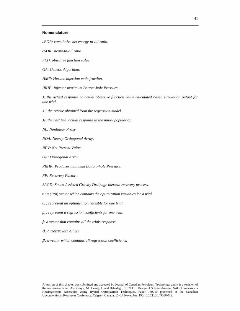
41
A version of this chapter was submitted and accepted by Journal of Canadian Petroleum Technology and it is a revision of
the conference paper: Al-Gosayir, M., Leung, J., and Babadagli, T., 2011b. Design of Solvent-Assisted SAGD Processes in Heterogeneous Reservoirs Using Hybrid Optimization Techniques. Paper 149010 presented at the Canadian
Unconventional Resources Conference, Calgary, Canada, 15–17 November. DOI: 10.2118/149010-MS.
Nomenclature
cEOR: cumulative net energy-to-oil ratio.
cSOR: steam-to-oil ratio.
F(X): objective function value.
GA: Genetic Algorithm.
HMF: Hexane injection mole fraction.
IBHP: Injector maximum Bottom-hole Pressure.
J: the actual response or actual objective function value calculated based simulation output for
one trial.
J’: the repose obtained from the regression model.
J0: the best trial actual response in the initial population.
NL: Nonlinear Proxy
NOA: Nearly-Orthogonal Array.
NPV: Net Present Value.
OA: Orthogonal Array.
PBHP: Producer minimum Bottom-hole Pressure.
RF: Recovery Factor.
SAGD: Steam Assisted Gravity Drainage thermal recovery process.
u: a (1*n) vector which contains the optimization variables for a trial.
ui : represent an optimization variable for one trial.
βi : represent a regression coefficients for one trial.
: a vector that contains all the trials response.
: a matrix with all u’s.
: a vector which contains all regression coefficients.
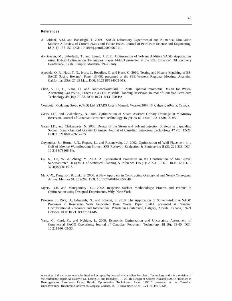
42
A version of this chapter was submitted and accepted by Journal of Canadian Petroleum Technology and it is a revision of
the conference paper: Al-Gosayir, M., Leung, J., and Babadagli, T., 2011b. Design of Solvent-Assisted SAGD Processes in Heterogeneous Reservoirs Using Hybrid Optimization Techniques. Paper 149010 presented at the Canadian
Unconventional Resources Conference, Calgary, Canada, 15–17 November. DOI: 10.2118/149010-MS.
References
Al-Bahlani, A.M. and Babadagli, T. 2009. SAGD Laboratory Experimental and Numerical Simulation
Studies: A Review of Current Status and Future Issues. Journal of Petroleum Science and Engineering,
68(3-4): 135-150. DOI: 10.1016/j.petrol.2009.06.011.
Al-Gosayir, M., Babadagli, T., and Leung, J. 2011. Optimization of Solvent Additive SAGD Applications
using Hybrid Optimization Techniques. Paper 144963 presented at the SPE Enhanced Oil Recovery
Conference, Kuala Lumpur, Malaysia, 19–21 July.
Ayodele, O. R., Nasr, T. N., Ivory, J., Beaulieu, G. and Heck, G. 2010. Testing and History Matching of ES-
SAGD (Using Hexane). Paper 134002 presented at the SPE Western Regional Meeting, Anaheim,
California, USA, 27-29 May. DOI: 10.2118/134002-MS.
Chen, S., Li, H., Yang, D., and Tontiwachwuthikul, P. 2010. Optimal Parametric Design for Water-
Alternating-Gas (WAG) Process in a CO2-Miscible Flooding Reservoir. Journal of Canadian Petroleum
Technology 49 (10): 75-82. DOI: 10.2118/141650-PA
ComputerModelingGroup(CMG)Ltd.STARSUser’sManual,Version2009.10.Calgary,Alberta,Canada.
Gates, I.D., and Chakrabarty, N. 2006. Optimization of Steam Assisted Gravity Drainage in McMurray
Reservoir. Journal of Canadian Petroleum Technology 45 (9): 55-62. DOI: 10.2118/06-09-05.
Gates, I.D., and Chakrabarty, N. 2008. Design of the Steam and Solvent Injection Strategy in Expanding
Solvent Steam-Assisted Gravity Drainage. Journal of Canadian Petroleum Technology 47 (9): 12-20.
DOI: 10.2118/08-09-12-CS.
Guyaguler, B., Horne, R.N., Rogers, L., and Rosenzweig, J.J. 2002. Optimization of Well Placement in a
Gulf of Mexico Waterflooding Project. SPE Reservoir Evaluation & Engineering 5 (3): 229-236. DOI:
10.2118/78266-PA.
Lu, X., Hu, W. & Zheng, Y. 2003. A Systematical Procedure in the Construction of Multi-Level
Supersaturated Designs. J. of Statistical Planning & Inference 115 (1): 287-310. DOI: 10.1016/S0378-
3758(02)00116-7.
Ma, C-X., Fang, K-T & Liski, E. 2000. A New Approach in Constructing Orthogonal and Nearly Orthogonal
Arrays. Metrika 50: 255-268. DOI: 10.1007/s001840050049.
Myers, R.H. and Montgomery D.C. 2002. Response Surface Methodology: Process and Product in
Optimization using Designed Experiments, Wily, New York.
Peterson, J., Riva, D., Edmunds, N., and Solanki, S. 2010. The Application of Solvent-Additive SAGD
Processes in Reservoirs With Associated Basal Water. Paper 137833 presented at Canadian
Unconventional Resources and International Petroleum Conference, Calgary, Alberta, Canada, 19-21
October. DOI: 10.2118/137833-MS.
Yang, C., Card, C., and Nghiem, L. 2009. Economic Optimization and Uncertainty Assessment of
Commercial SAGD Operations. Journal of Canadian Petroleum Technology 48 (9): 33-40. DOI:
10.2118/09-09-33.
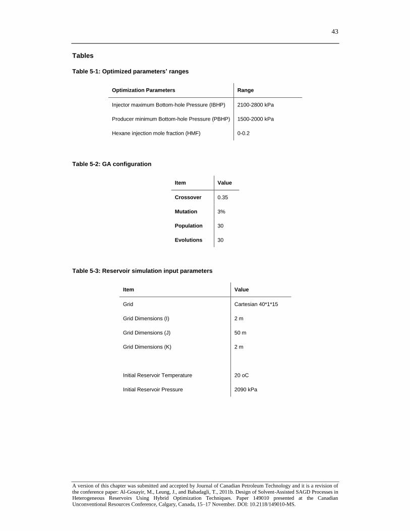
43
A version of this chapter was submitted and accepted by Journal of Canadian Petroleum Technology and it is a revision of
the conference paper: Al-Gosayir, M., Leung, J., and Babadagli, T., 2011b. Design of Solvent-Assisted SAGD Processes in Heterogeneous Reservoirs Using Hybrid Optimization Techniques. Paper 149010 presented at the Canadian
Unconventional Resources Conference, Calgary, Canada, 15–17 November. DOI: 10.2118/149010-MS.
Tables
Table 5-1: Optimized parameters’ ranges
Optimization Parameters Range
Injector maximum Bottom-hole Pressure (IBHP) 2100-2800 kPa
Producer minimum Bottom-hole Pressure (PBHP) 1500-2000 kPa
Hexane injection mole fraction (HMF) 0-0.2
Table 5-2: GA configuration
Item Value
Crossover 0.35
Mutation 3%
Population 30
Evolutions 30
Table 5-3: Reservoir simulation input parameters
Item Value
Grid Cartesian 40*1*15
Grid Dimensions (I) 2 m
Grid Dimensions (J) 50 m
Grid Dimensions (K) 2 m
Initial Reservoir Temperature 20 oC
Initial Reservoir Pressure 2090 kPa
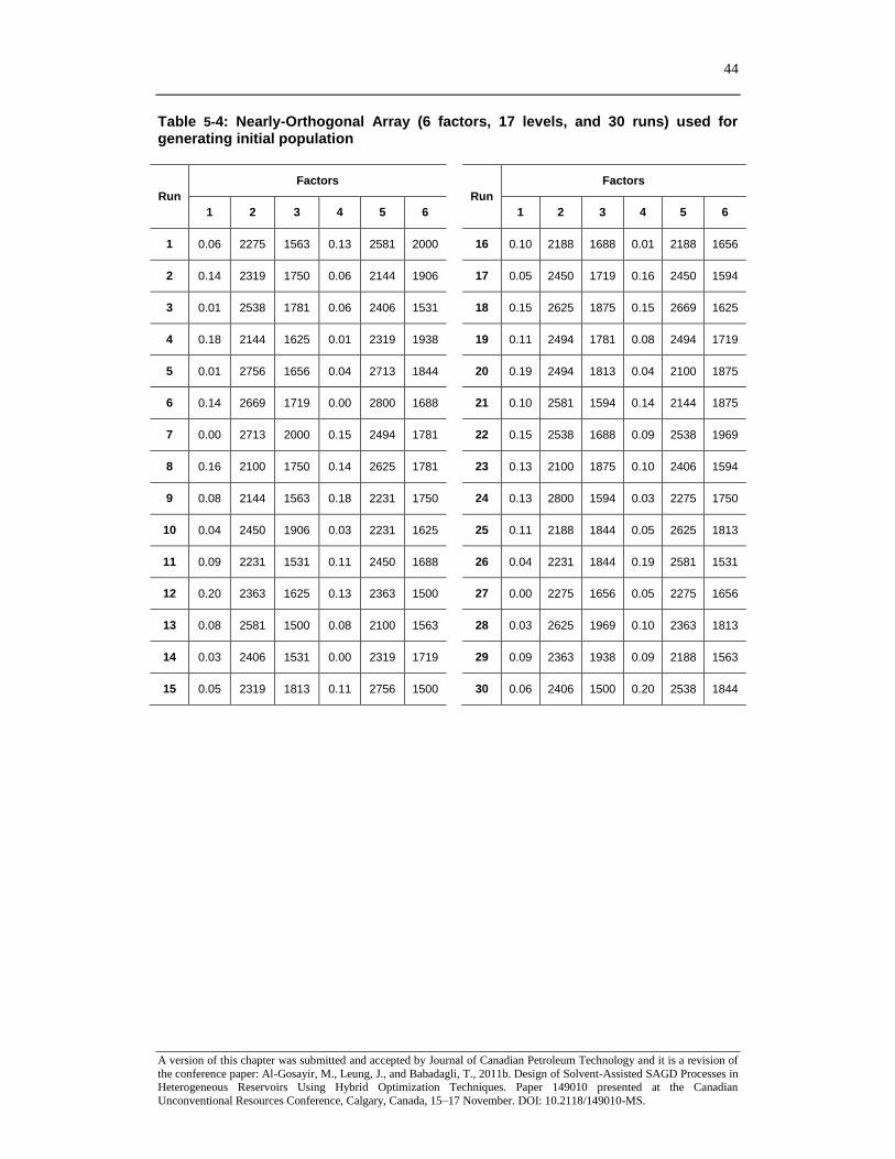
44
A version of this chapter was submitted and accepted by Journal of Canadian Petroleum Technology and it is a revision of
the conference paper: Al-Gosayir, M., Leung, J., and Babadagli, T., 2011b. Design of Solvent-Assisted SAGD Processes in Heterogeneous Reservoirs Using Hybrid Optimization Techniques. Paper 149010 presented at the Canadian
Unconventional Resources Conference, Calgary, Canada, 15–17 November. DOI: 10.2118/149010-MS.
Table 5-4: Nearly-Orthogonal Array (6 factors, 17 levels, and 30 runs) used for generating initial population
Run
Factors
Run
Factors
1 2 3 4 5 6 1 2 3 4 5 6
1 0.06 2275 1563 0.13 2581 2000 16 0.10 2188 1688 0.01 2188 1656
2 0.14 2319 1750 0.06 2144 1906 17 0.05 2450 1719 0.16 2450 1594
3 0.01 2538 1781 0.06 2406 1531 18 0.15 2625 1875 0.15 2669 1625
4 0.18 2144 1625 0.01 2319 1938 19 0.11 2494 1781 0.08 2494 1719
5 0.01 2756 1656 0.04 2713 1844 20 0.19 2494 1813 0.04 2100 1875
6 0.14 2669 1719 0.00 2800 1688 21 0.10 2581 1594 0.14 2144 1875
7 0.00 2713 2000 0.15 2494 1781 22 0.15 2538 1688 0.09 2538 1969
8 0.16 2100 1750 0.14 2625 1781 23 0.13 2100 1875 0.10 2406 1594
9 0.08 2144 1563 0.18 2231 1750 24 0.13 2800 1594 0.03 2275 1750
10 0.04 2450 1906 0.03 2231 1625 25 0.11 2188 1844 0.05 2625 1813
11 0.09 2231 1531 0.11 2450 1688 26 0.04 2231 1844 0.19 2581 1531
12 0.20 2363 1625 0.13 2363 1500 27 0.00 2275 1656 0.05 2275 1656
13 0.08 2581 1500 0.08 2100 1563 28 0.03 2625 1969 0.10 2363 1813
14 0.03 2406 1531 0.00 2319 1719 29 0.09 2363 1938 0.09 2188 1563
15 0.05 2319 1813 0.11 2756 1500 30 0.06 2406 1500 0.20 2538 1844
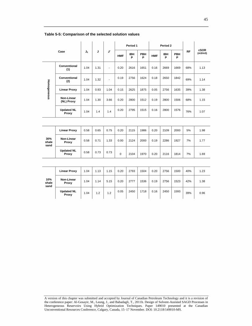
45
A version of this chapter was submitted and accepted by Journal of Canadian Petroleum Technology and it is a revision of
the conference paper: Al-Gosayir, M., Leung, J., and Babadagli, T., 2011b. Design of Solvent-Assisted SAGD Processes in Heterogeneous Reservoirs Using Hybrid Optimization Techniques. Paper 149010 presented at the Canadian
Unconventional Resources Conference, Calgary, Canada, 15–17 November. DOI: 10.2118/149010-MS.
Table 5-5: Comparison of the selected solution values
Case J0 J J’
Period 1 Period 2
RF cSOR
(m3/m3) HMF
IBHP
PBHP
HMF IBHP
PBHP
Ho
mo
ge
ne
ou
s
Conventional (1)
1.04 1.31 - 0.20 2616 1651 0.16 2669 1669 68% 1.13
Conventional (2)
1.04 1.32 - 0.19 2756 1624 0.18 2650 1842
69% 1.14
Linear Proxy 1.04 0.93 1.04 0.15 2625 1875 0.05 2756 1635 39% 1.38
Non-Linear (NL) Proxy
1.04 1.30 3.66 0.20 2800 1512 0.19 2800 1506 68% 1.15
Updated NL Proxy
1.04 1.4 1.4 0.20 2795 1515 0.16 2800 1576
76% 1.07
30% shale sand
Linear Proxy 0.58 0.65 0.75 0.20 2115 1986 0.20 2109 2000 5% 1.98
Non-Linear Proxy
0.58 0.71 1.33 0.00 2124 2000 0.19 2286 1927 7% 1.77
Updated NL Proxy
0.58 0.73 0.73 0 2104 1970 0.20 2116 1814 7% 1.69
10% shale sand
Linear Proxy 1.04 1.13 1.15 0.20 2793 1504 0.20 2756 1500 40% 1.23
Non-Linear Proxy
1.04 1.14 5.15 0.20 2777 1536 0.19 2756 1523 42% 1.38
Updated NL Proxy
1.04 1.2 1.2 0.05 2450 1718 0.16 2450 1593
39% 0.96
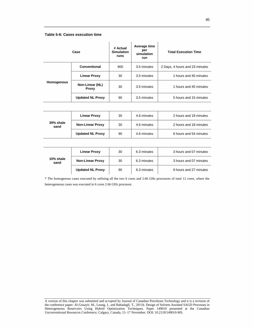
46
A version of this chapter was submitted and accepted by Journal of Canadian Petroleum Technology and it is a revision of
the conference paper: Al-Gosayir, M., Leung, J., and Babadagli, T., 2011b. Design of Solvent-Assisted SAGD Processes in Heterogeneous Reservoirs Using Hybrid Optimization Techniques. Paper 149010 presented at the Canadian
Unconventional Resources Conference, Calgary, Canada, 15–17 November. DOI: 10.2118/149010-MS.
Table 5-6: Cases execution time
Case # Actual
Simulation runs
Average time per
simulation run
Total Execution Time
Homogenous
Conventional 900 3.5 minutes 2 Days, 4 hours and 23 minutes
Linear Proxy 30 3.5 minutes 1 hours and 45 minutes
Non-Linear (NL) Proxy
30 3.5 minutes 1 hours and 45 minutes
Updated NL Proxy 90 3.5 minutes 5 hours and 15 minutes
30% shale sand
Linear Proxy 30 4.6 minutes 2 hours and 18 minutes
Non-Linear Proxy 30 4.6 minutes 2 hours and 18 minutes
Updated NL Proxy 90 4.6 minutes 6 hours and 54 minutes
10% shale sand
Linear Proxy 30 6.3 minutes 3 hours and 07 minutes
Non-Linear Proxy 30 6.3 minutes 3 hours and 07 minutes
Updated NL Proxy 90 6.3 minutes 9 hours and 27 minutes
* The homogenous cases executed by utilizing all the two 6 cores and 2.66 GHz processors of total 12 cores, where the
heterogeneous cases was executed in 6 cores 2.66 GHz processor.
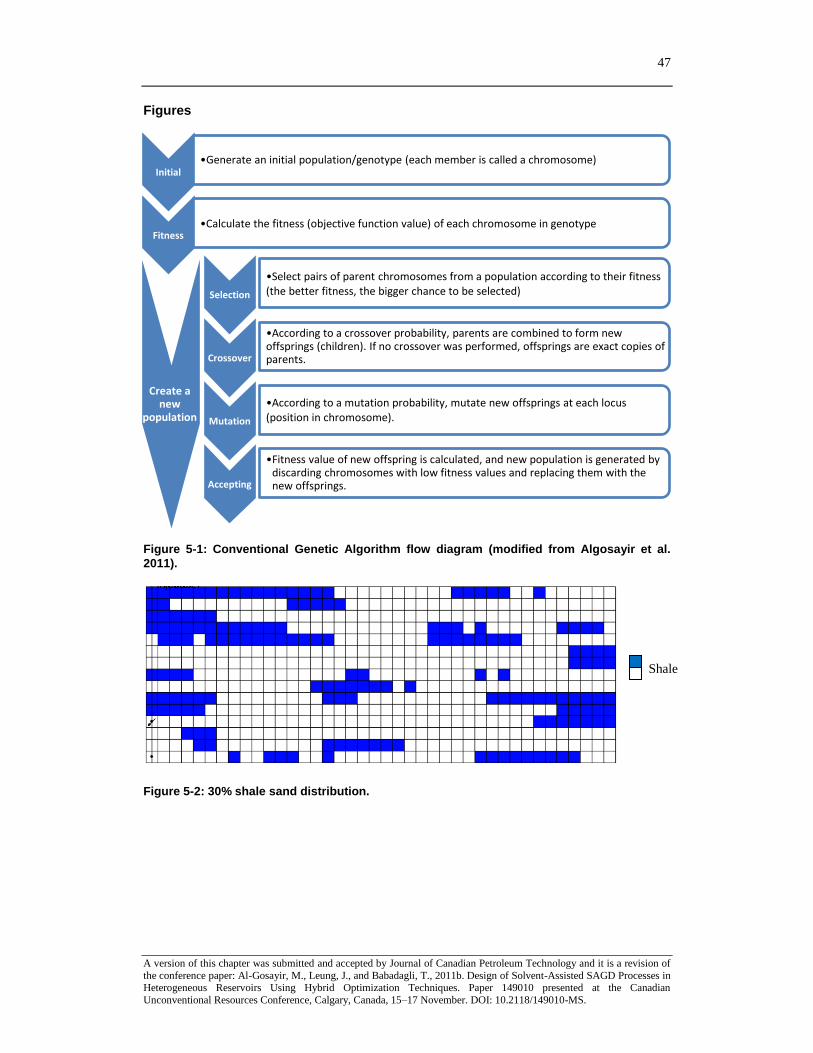
47
A version of this chapter was submitted and accepted by Journal of Canadian Petroleum Technology and it is a revision of
the conference paper: Al-Gosayir, M., Leung, J., and Babadagli, T., 2011b. Design of Solvent-Assisted SAGD Processes in Heterogeneous Reservoirs Using Hybrid Optimization Techniques. Paper 149010 presented at the Canadian
Unconventional Resources Conference, Calgary, Canada, 15–17 November. DOI: 10.2118/149010-MS.
Figures
Figure 5-1: Conventional Genetic Algorithm flow diagram (modified from Algosayir et al.
2011).
Figure 5-2: 30% shale sand distribution.
Initial •Generate an initial population/genotype (each member is called a chromosome)
Fitness •Calculate the fitness (objective function value) of each chromosome in genotype
Selection
•Select pairs of parent chromosomes from a population according to their fitness (the better fitness, the bigger chance to be selected)
Crossover
•According to a crossover probability, parents are combined to form new offsprings (children). If no crossover was performed, offsprings are exact copies of parents.
Mutation
•According to a mutation probability, mutate new offsprings at each locus (position in chromosome).
Accepting
•Fitness value of new offspring is calculated, and new population is generated by discarding chromosomes with low fitness values and replacing them with the new offsprings.
Create a new
population
Shale
Sand
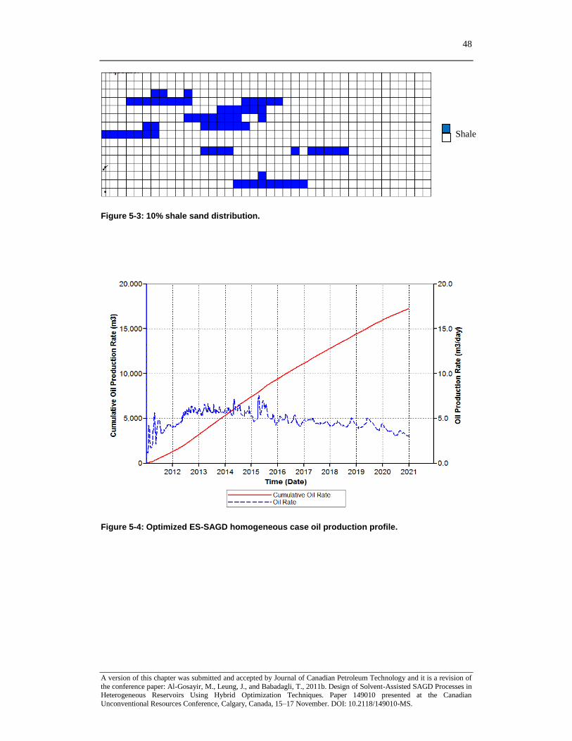
48
A version of this chapter was submitted and accepted by Journal of Canadian Petroleum Technology and it is a revision of
the conference paper: Al-Gosayir, M., Leung, J., and Babadagli, T., 2011b. Design of Solvent-Assisted SAGD Processes in Heterogeneous Reservoirs Using Hybrid Optimization Techniques. Paper 149010 presented at the Canadian
Unconventional Resources Conference, Calgary, Canada, 15–17 November. DOI: 10.2118/149010-MS.
Figure 5-3: 10% shale sand distribution.
Figure 5-4: Optimized ES-SAGD homogeneous case oil production profile.
Shale
Sand
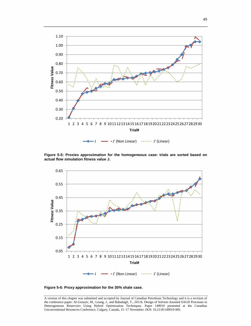
49
A version of this chapter was submitted and accepted by Journal of Canadian Petroleum Technology and it is a revision of
the conference paper: Al-Gosayir, M., Leung, J., and Babadagli, T., 2011b. Design of Solvent-Assisted SAGD Processes in Heterogeneous Reservoirs Using Hybrid Optimization Techniques. Paper 149010 presented at the Canadian
Unconventional Resources Conference, Calgary, Canada, 15–17 November. DOI: 10.2118/149010-MS.
Figure 5-5: Proxies approximation for the homogeneous case: trials are sorted based on
actual flow simulation fitness value J.
Figure 5-6: Proxy approximation for the 30% shale case.
0.20
0.30
0.40
0.50
0.60
0.70
0.80
0.90
1.00
1.10
1 2 3 4 5 6 7 8 9 101112131415161718192021222324252627282930
Fitn
ess
Val
ue
Trial#
J J' (Non Linear) J' (Linear)
0.05
0.15
0.25
0.35
0.45
0.55
0.65
1 2 3 4 5 6 7 8 9 101112131415161718192021222324252627282930
Fitn
ess
Val
ue
Trial#
J J' (Non Linear) J' (Linear)
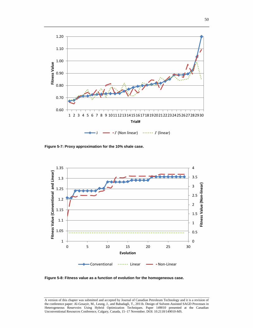
50
A version of this chapter was submitted and accepted by Journal of Canadian Petroleum Technology and it is a revision of
the conference paper: Al-Gosayir, M., Leung, J., and Babadagli, T., 2011b. Design of Solvent-Assisted SAGD Processes in Heterogeneous Reservoirs Using Hybrid Optimization Techniques. Paper 149010 presented at the Canadian
Unconventional Resources Conference, Calgary, Canada, 15–17 November. DOI: 10.2118/149010-MS.
Figure 5-7: Proxy approximation for the 10% shale case.
Figure 5-8: Fitness value as a function of evolution for the homogeneous case.
0.60
0.70
0.80
0.90
1.00
1.10
1.20
1 2 3 4 5 6 7 8 9 101112131415161718192021222324252627282930
Fitn
ess
Val
ue
Trial#
J J' (Non linear) J' (linear)
0
0.5
1
1.5
2
2.5
3
3.5
4
1
1.05
1.1
1.15
1.2
1.25
1.3
1.35
0 5 10 15 20 25 30
Fitn
ess
Val
ue
(N
on
-lin
ear
)
Fitn
ess
Val
ue
(C
on
ven
tio
nal
an
d L
ine
ar)
Evolution
Conventional Linear Non-Linear
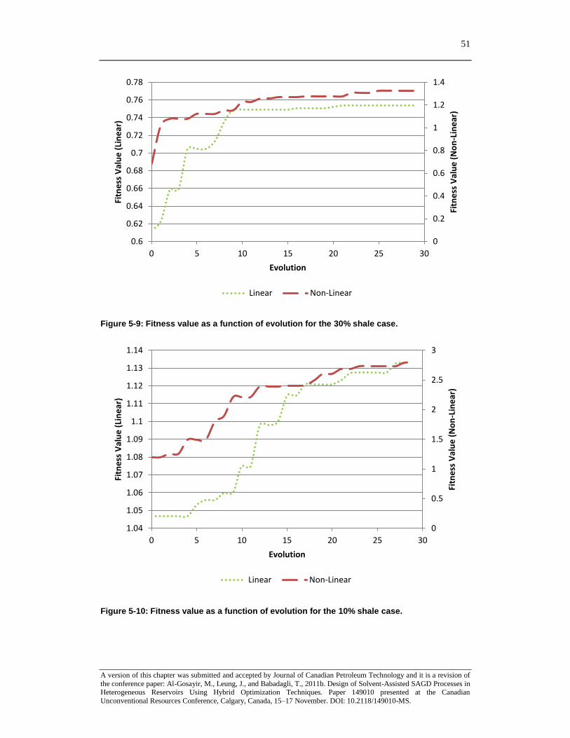
51
A version of this chapter was submitted and accepted by Journal of Canadian Petroleum Technology and it is a revision of
the conference paper: Al-Gosayir, M., Leung, J., and Babadagli, T., 2011b. Design of Solvent-Assisted SAGD Processes in Heterogeneous Reservoirs Using Hybrid Optimization Techniques. Paper 149010 presented at the Canadian
Unconventional Resources Conference, Calgary, Canada, 15–17 November. DOI: 10.2118/149010-MS.
Figure 5-9: Fitness value as a function of evolution for the 30% shale case.
Figure 5-10: Fitness value as a function of evolution for the 10% shale case.
0
0.2
0.4
0.6
0.8
1
1.2
1.4
0.6
0.62
0.64
0.66
0.68
0.7
0.72
0.74
0.76
0.78
0 5 10 15 20 25 30
Fitn
ess
Val
ue
(N
on
-Lin
ear
)
Fitn
ess
Val
ue
(Li
ne
ar)
Evolution
Linear Non-Linear
0
0.5
1
1.5
2
2.5
3
1.04
1.05
1.06
1.07
1.08
1.09
1.1
1.11
1.12
1.13
1.14
0 5 10 15 20 25 30
Fitn
ess
Val
ue
(N
on
-Lin
ear
)
Fitn
ess
Val
ue
(Li
ne
ar)
Evolution
Linear Non-Linear
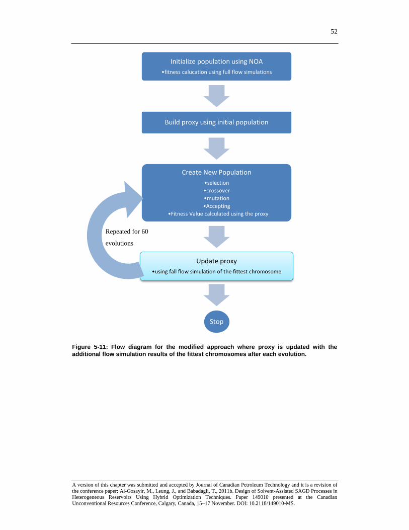
52
A version of this chapter was submitted and accepted by Journal of Canadian Petroleum Technology and it is a revision of
the conference paper: Al-Gosayir, M., Leung, J., and Babadagli, T., 2011b. Design of Solvent-Assisted SAGD Processes in Heterogeneous Reservoirs Using Hybrid Optimization Techniques. Paper 149010 presented at the Canadian
Unconventional Resources Conference, Calgary, Canada, 15–17 November. DOI: 10.2118/149010-MS.
Figure 5-11: Flow diagram for the modified approach where proxy is updated with the
additional flow simulation results of the fittest chromosomes after each evolution.
Initialize population using NOA
•fitness calucation using full flow simulations
Build proxy using initial population
Create New Population
•selection
•crossover
•mutation
•Accepting
•Fitness Value calculated using the proxy
Update proxy
•using fall flow simulation of the fittest chromosome
Stop
Repeated for 60
evolutions
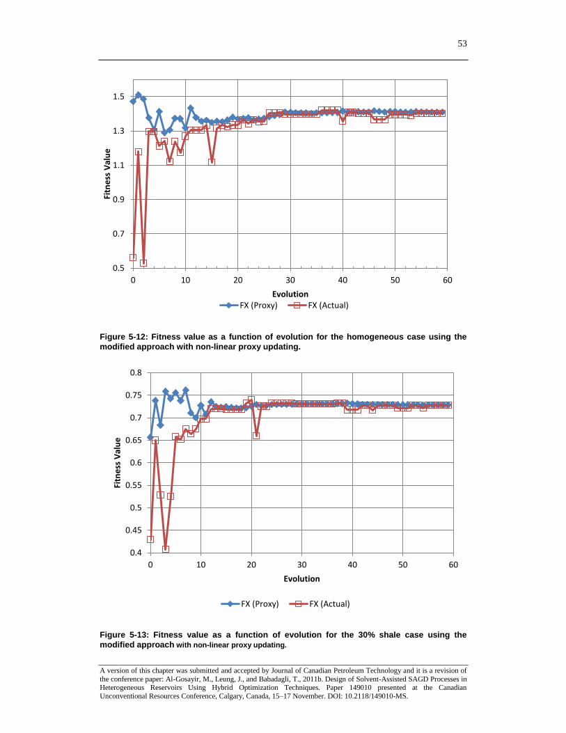
53
A version of this chapter was submitted and accepted by Journal of Canadian Petroleum Technology and it is a revision of
the conference paper: Al-Gosayir, M., Leung, J., and Babadagli, T., 2011b. Design of Solvent-Assisted SAGD Processes in Heterogeneous Reservoirs Using Hybrid Optimization Techniques. Paper 149010 presented at the Canadian
Unconventional Resources Conference, Calgary, Canada, 15–17 November. DOI: 10.2118/149010-MS.
Figure 5-12: Fitness value as a function of evolution for the homogeneous case using the
modified approach with non-linear proxy updating.
Figure 5-13: Fitness value as a function of evolution for the 30% shale case using the
modified approach with non-linear proxy updating.
0.5
0.7
0.9
1.1
1.3
1.5
0 10 20 30 40 50 60
Fitn
ess
Val
ue
Evolution FX (Proxy) FX (Actual)
0.4
0.45
0.5
0.55
0.6
0.65
0.7
0.75
0.8
0 10 20 30 40 50 60
Fitn
ess
Val
ue
Evolution
FX (Proxy) FX (Actual)
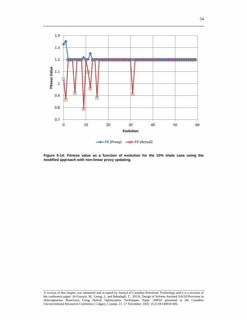
54
A version of this chapter was submitted and accepted by Journal of Canadian Petroleum Technology and it is a revision of
the conference paper: Al-Gosayir, M., Leung, J., and Babadagli, T., 2011b. Design of Solvent-Assisted SAGD Processes in Heterogeneous Reservoirs Using Hybrid Optimization Techniques. Paper 149010 presented at the Canadian
Unconventional Resources Conference, Calgary, Canada, 15–17 November. DOI: 10.2118/149010-MS.
Figure 5-14: Fitness value as a function of evolution for the 10% shale case using the
modified approach with non-linear proxy updating.
0.7
0.8
0.9
1
1.1
1.2
1.3
1.4
0 10 20 30 40 50 60
Fitn
ess
Val
ue
Evolution
FX (Proxy) FX (Actual)

55
A version of this chapter was submitted for publication.
Chapter 6: Optimization of SOS-FR (Steam-Over-Solvent Injection in Fractured Reservoirs) Method Using Hybrid Techniques: Testing Cyclic Injection
Case
Abstract
Many processes and techniques have been proposed to improve the heavy oil recovery from
fractured reservoirs. Such complex processes require careful operation planning and management
to achieve optimal efficiency with minimal costs and environmental impacts. Steam injection is
one of the options for heavy-oil recovery from fractured reservoirs but significant steam
requirement for effective matrix heating due to heterogeneous structure poses important challenges
in terms of cost, water availability, and environment impacts due to water processing and steam
generation. Al-Bahlani and Babadagli (2008, 2009a) proposed a new process called Steam-Over-
Solvent in Fractured Reservoirs (SOS-FR) by adding solvent component to minimize the heat
needed. The SOS-FR technique consists of a heating phase using steam injection, subsequent
solvent injection, and low temperature steam injection for solvent retrieval and additional oil
recovery. Optimization of this process is a critical step to determine optimal injection (and
soaking) schedules as the heterogeneous structure of this kind of reservoirs may easily yield an
inefficient process due to high cost and excessive use of steam and solvent. In this study, we
adopted a global optimization scheme, where genetic algorithm is integrated with orthogonal
arrays and response surface proxies for better convergence behavior and higher computational
efficiency, to optimize the SOS-FR process for cyclic injection option. The results show that one
may be able to double the profit obtained with the benchmark model using the optimal injection
scheme suggested by our optimization procedure.
Introduction
Unconventional solutions are needed to overcome the challenge of heavy oil production. In high
permeability non-fractured sand reservoirs, steam injection processes showed acceptable
production, however, they require the availability of a large amount of water that is a major
challenge in remote areas with limited water accessibility, and this water consumption has to be
managed and processed in an environment friendly manner (Al-Bahlani and Babadagli, 2011).
Alternative to steam injection, Butler and Mokrys (1991) introduced the VAPEX (vapor
extraction) process, which is pure solvent injection from a horizontal well to displace the oil by
gravity drainage to another horizontal producer. Later, different schemes of steam/solvent
injection were tested at laboratory or simulation conditions as well as field pilots. Nasr et al.
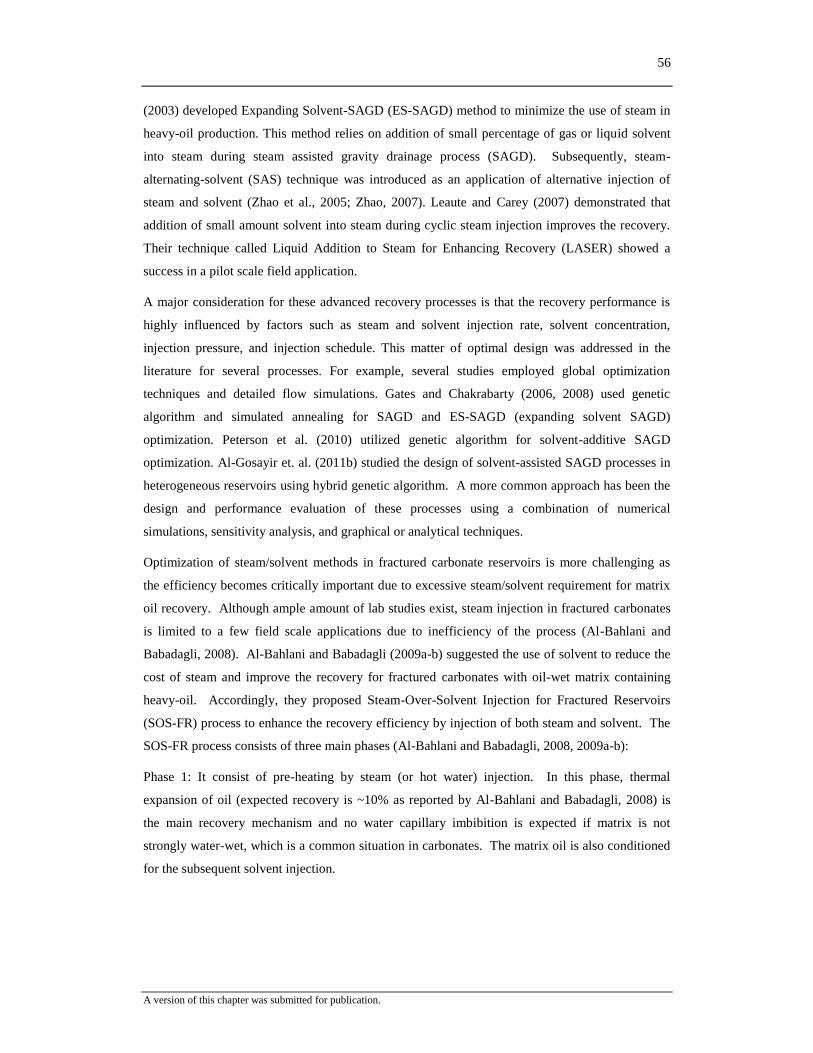
56
A version of this chapter was submitted for publication.
(2003) developed Expanding Solvent-SAGD (ES-SAGD) method to minimize the use of steam in
heavy-oil production. This method relies on addition of small percentage of gas or liquid solvent
into steam during steam assisted gravity drainage process (SAGD). Subsequently, steam-
alternating-solvent (SAS) technique was introduced as an application of alternative injection of
steam and solvent (Zhao et al., 2005; Zhao, 2007). Leaute and Carey (2007) demonstrated that
addition of small amount solvent into steam during cyclic steam injection improves the recovery.
Their technique called Liquid Addition to Steam for Enhancing Recovery (LASER) showed a
success in a pilot scale field application.
A major consideration for these advanced recovery processes is that the recovery performance is
highly influenced by factors such as steam and solvent injection rate, solvent concentration,
injection pressure, and injection schedule. This matter of optimal design was addressed in the
literature for several processes. For example, several studies employed global optimization
techniques and detailed flow simulations. Gates and Chakrabarty (2006, 2008) used genetic
algorithm and simulated annealing for SAGD and ES-SAGD (expanding solvent SAGD)
optimization. Peterson et al. (2010) utilized genetic algorithm for solvent-additive SAGD
optimization. Al-Gosayir et. al. (2011b) studied the design of solvent-assisted SAGD processes in
heterogeneous reservoirs using hybrid genetic algorithm. A more common approach has been the
design and performance evaluation of these processes using a combination of numerical
simulations, sensitivity analysis, and graphical or analytical techniques.
Optimization of steam/solvent methods in fractured carbonate reservoirs is more challenging as
the efficiency becomes critically important due to excessive steam/solvent requirement for matrix
oil recovery. Although ample amount of lab studies exist, steam injection in fractured carbonates
is limited to a few field scale applications due to inefficiency of the process (Al-Bahlani and
Babadagli, 2008). Al-Bahlani and Babadagli (2009a-b) suggested the use of solvent to reduce the
cost of steam and improve the recovery for fractured carbonates with oil-wet matrix containing
heavy-oil. Accordingly, they proposed Steam-Over-Solvent Injection for Fractured Reservoirs
(SOS-FR) process to enhance the recovery efficiency by injection of both steam and solvent. The
SOS-FR process consists of three main phases (Al-Bahlani and Babadagli, 2008, 2009a-b):
Phase 1: It consist of pre-heating by steam (or hot water) injection. In this phase, thermal
expansion of oil (expected recovery is ~10% as reported by Al-Bahlani and Babadagli, 2008) is
the main recovery mechanism and no water capillary imbibition is expected if matrix is not
strongly water-wet, which is a common situation in carbonates. The matrix oil is also conditioned
for the subsequent solvent injection.
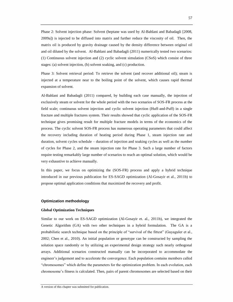
57
A version of this chapter was submitted for publication.
Phase 2: Solvent injection phase: Solvent (heptane was used by Al-Bahlani and Babadagli [2008,
2009a]) is injected to be diffused into matrix and further reduce the viscosity of oil. Then, the
matrix oil is produced by gravity drainage caused by the density difference between original oil
and oil diluted by the solvent. Al-Bahlani and Babadagli (2011) numerically tested two scenarios:
(1) Continuous solvent injection and (2) cyclic solvent simulation (CSoS) which consist of three
stages: (a) solvent injection, (b) solvent soaking, and (c) production.
Phase 3: Solvent retrieval period: To retrieve the solvent (and recover additional oil); steam is
injected at a temperature near to the boiling point of the solvent, which causes rapid thermal
expansion of solvent.
Al-Bahlani and Babadagli (2011) compared, by building each case manually, the injection of
exclusively steam or solvent for the whole period with the two scenarios of SOS-FR process at the
field scale; continuous solvent injection and cyclic solvent injection (Huff-and-Puff) in a single
fracture and multiple fractures system. Their results showed that cyclic application of the SOS-FR
technique gives promising result for multiple fracture models in terms of the economics of the
process. The cyclic solvent SOS-FR process has numerous operating parameters that could affect
the recovery including duration of heating period during Phase 1, steam injection rate and
duration, solvent cycles schedule – duration of injection and soaking cycles as well as the number
of cycles for Phase 2, and the steam injection rate for Phase 3. Such a large number of factors
require testing remarkably large number of scenarios to reach an optimal solution, which would be
very exhaustive to achieve manually.
In this paper, we focus on optimizing the (SOS-FR) process and apply a hybrid technique
introduced in our previous publication for ES-SAGD optimization (Al-Gosayir et al., 2011b) to
propose optimal application conditions that maximized the recovery and profit.
Optimization methodology
Global Optimization Techniques
Similar to our work on ES-SAGD optimization (Al-Gosayir et. al., 2011b), we integrated the
Genetic Algorithm (GA) with two other techniques in a hybrid formulation. The GA is a
probabilisticsearchtechniquebasedontheprincipleof“survivalofthefittest”(Guyaguleretal.,
2002; Chen et al., 2010). An initial population or genotype can be constructed by sampling the
solution space randomly or by utilizing an experimental design strategy such nearly orthogonal
arrays. Additional scenarios constructed manually can be incorporated to accommodate the
engineer’sjudgementandtoacceleratetheconvergence.Eachpopulationcontainsmemberscalled
“chromosomes”whichdefinetheparametersfortheoptimizationproblem.Ineachevolution,each
chromosome’sfitness is calculated. Then, pairs of parent chromosomes are selected based on their
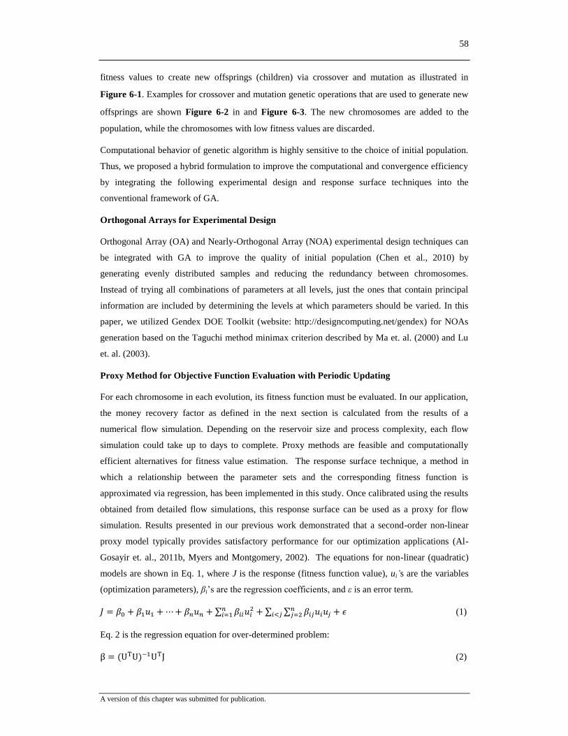
58
A version of this chapter was submitted for publication.
fitness values to create new offsprings (children) via crossover and mutation as illustrated in
Figure 6-1. Examples for crossover and mutation genetic operations that are used to generate new
offsprings are shown Figure 6-2 in and Figure 6-3. The new chromosomes are added to the
population, while the chromosomes with low fitness values are discarded.
Computational behavior of genetic algorithm is highly sensitive to the choice of initial population.
Thus, we proposed a hybrid formulation to improve the computational and convergence efficiency
by integrating the following experimental design and response surface techniques into the
conventional framework of GA.
Orthogonal Arrays for Experimental Design
Orthogonal Array (OA) and Nearly-Orthogonal Array (NOA) experimental design techniques can
be integrated with GA to improve the quality of initial population (Chen et al., 2010) by
generating evenly distributed samples and reducing the redundancy between chromosomes.
Instead of trying all combinations of parameters at all levels, just the ones that contain principal
information are included by determining the levels at which parameters should be varied. In this
paper, we utilized Gendex DOE Toolkit (website: http://designcomputing.net/gendex) for NOAs
generation based on the Taguchi method minimax criterion described by Ma et. al. (2000) and Lu
et. al. (2003).
Proxy Method for Objective Function Evaluation with Periodic Updating
For each chromosome in each evolution, its fitness function must be evaluated. In our application,
the money recovery factor as defined in the next section is calculated from the results of a
numerical flow simulation. Depending on the reservoir size and process complexity, each flow
simulation could take up to days to complete. Proxy methods are feasible and computationally
efficient alternatives for fitness value estimation. The response surface technique, a method in
which a relationship between the parameter sets and the corresponding fitness function is
approximated via regression, has been implemented in this study. Once calibrated using the results
obtained from detailed flow simulations, this response surface can be used as a proxy for flow
simulation. Results presented in our previous work demonstrated that a second-order non-linear
proxy model typically provides satisfactory performance for our optimization applications (Al-
Gosayir et. al., 2011b, Myers and Montgomery, 2002). The equations for non-linear (quadratic)
models are shown in Eq. 1, where J is the response (fitness function value), ui’s are the variables
(optimization parameters), βi’saretheregressioncoefficients,andε is an error term.
∑
∑ ∑ (1)
Eq. 2 is the regression equation for over-determined problem:
(2)

59
A version of this chapter was submitted for publication.
When the number of optimization parameters is larger than the number of experiments, the
problem becomes under-determined and Eq. 3 should be used:
(3)
where is a vector that contains all the response, is a vector which contains all regression
coefficients and is a matrix with all the u vectors evaluated.
In order to achieve a better representation of the solution space and regression accuracy, the proxy
is re-calibrated or updated periodically by performing detailed flow simulation using parameters of
the chromosome with the highest fitness value and incorporating its simulation result after each
evolution (Al-Gosayir et al., 2011b). This updating step is illustrated in the flow chart given in
Figure 6-4.
In this research, we used the JGAP package (Java Genetic Algorithm Package (JGAP) website:
http://jgap.sourceforge.net/) for the GA modeling.
Objective Function
Efficiency of recovery processes can be assessed by their profit by calculating the Money
Recovery Factor, MRF, (Al-Bahlani and Babadagli, 2011) which incorporate the major elements
(mainly steam, solvent, and oil), which influence the profit. The MRF focuses on the key
elements and omits the other factors, which may vary from one field to another. The MRF is
defined as follows:
where the cost is:
and the revenue is:
The steam cost and solvent and oil prices are shown in Table 6-1.
This objective function eliminates the revenue of the steam since it is not a common practice to
treat the produced water and re-inject it again as steam. One the other hand, solvent is considered
to have the same price for revenue and cost even if it is not extracted from the oil because it
upgrades the oil and reduces the need to add solvent for pipeline transportation and it is recovered

60
A version of this chapter was submitted for publication.
in the distillation tower. The capital expenditures (CAPEX) are considered the same for all
scenarios (Al-Bahlani and Babadagli, 2011).
Benchmark (Base) Simulation Model
Since Al-Bahlani and Babadagli (2011), results indicated that cyclic solvent SOS-FR in reservoirs
with multiple fractures yielded the highest money recovery factor (see Figure 16 of this reference),
we considered this as a base case for our optimization study. This model is an IK Cartesian 2D
single porosity-single permeability model with the dimensions of 20×30×15 m that contains
multiple fractures of 1 cm aperture. Geological features of the model are provided in Table 6-2.
Representation of the fracture-matrix model in a flow simulation is shown in Figure 6-5. This
base case gives a money recovery factor (MRF) value of approximately 28. This base case gives a
money recovery factor (MRF) value of approximately 28. This model was an implementation of
cyclic option of the SOS-FR Process. This model has total process duration of three years and six
months, and it is designed as follows (Al-Bahlani and Babadagli, 2011):
1. Phase 1: Heating period (HP) has 395 days length.
2. Phase 1: Heating period where steam is injected with rate of 20 m3/day.
3. Phase 1: Cooling period (CP) has 175 days length with cold-water injection with rate of 5
m3/day. This was included by Al-Bahlani and Babadagli (2001) in their simulation to
simulate their laboratory experiments (Al-Bahlani and Babadagli, 2008, 2009a), which
had a cooling period between Phase 1 (heating) and Phase 2 (solvent injection). In
practice, this corresponds to the period switching to Phase 2 and a short period of soaking
the reservoir with injected steam to condition the matrix oil for solvent diffusion.
4. Wells shut-in after the cooling period for 6 days.
5. Phase 2: 14 Cycles each cycle contains three periods: One week solvent injection, two
weeks soaking, and two weeks production.
6. Phase 3: Recovery phase where the steam is injected with rate of 20 m3/day.
7. Phase 3: Recovery phase length is 198 days.
Semi-compositional commercial simulator (CMG STARS) was used for full flow simulations
evaluation.
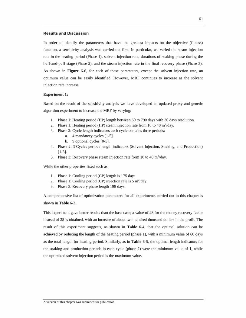
61
A version of this chapter was submitted for publication.
Results and Discussion
In order to identify the parameters that have the greatest impacts on the objective (fitness)
function, a sensitivity analysis was carried out first. In particular, we varied the steam injection
rate in the heating period (Phase 1), solvent injection rate, durations of soaking phase during the
huff-and-puff stage (Phase 2), and the steam injection rate in the final recovery phase (Phase 3).
As shown in Figure 6-6, for each of these parameters, except the solvent injection rate, an
optimum value can be easily identified. However, MRF continues to increase as the solvent
injection rate increase.
Experiment 1:
Based on the result of the sensitivity analysis we have developed an updated proxy and genetic
algorithm experiment to increase the MRF by varying:
1. Phase 1: Heating period (HP) length between 60 to 790 days with 30 days resolution.
2. Phase 1: Heating period (HP) steam injection rate from 10 to 40 m3/day.
3. Phase 2: Cycle length indicators each cycle contains three periods:
a. 4 mandatory cycles [1-5].
b. 9 optional cycles [0-5].
4. Phase 2: 3 Cycles periods length indicators (Solvent Injection, Soaking, and Production)
[1-3].
5. Phase 3: Recovery phase steam injection rate from 10 to 40 m3/day.
While the other properties fixed such as:
1. Phase 1: Cooling period (CP) length is 175 days
2. Phase 1: Cooling period (CP) injection rate is 5 m3/day.
3. Phase 3: Recovery phase length 198 days.
A comprehensive list of optimization parameters for all experiments carried out in this chapter is
shown in Table 6-3.
This experiment gave better results than the base case; a value of 48 for the money recovery factor
instead of 28 is obtained, with an increase of about two hundred thousand dollars in the profit. The
result of this experiment suggests, as shown in Table 6-4, that the optimal solution can be
achieved by reducing the length of the heating period (phase 1), with a minimum value of 60 days
as the total length for heating period. Similarly, as in Table 6-5, the optimal length indicators for
the soaking and production periods in each cycle (phase 2) were the minimum value of 1, while
the optimized solvent injection period is the maximum value.
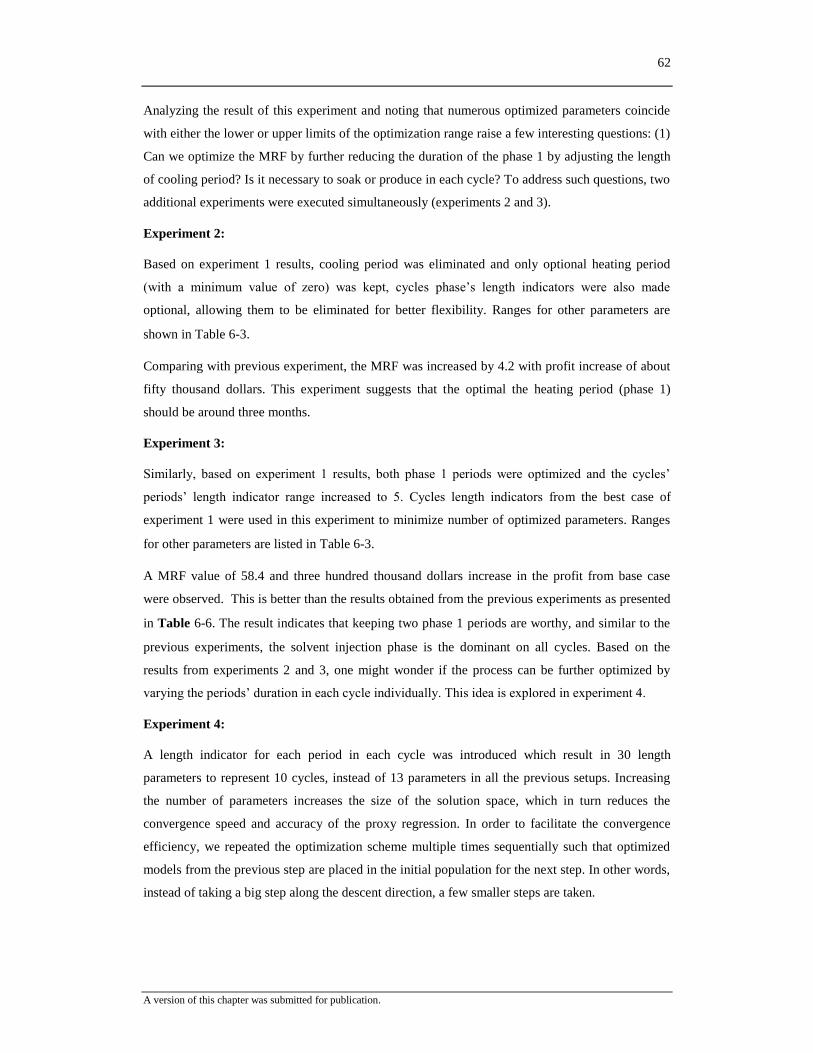
62
A version of this chapter was submitted for publication.
Analyzing the result of this experiment and noting that numerous optimized parameters coincide
with either the lower or upper limits of the optimization range raise a few interesting questions: (1)
Can we optimize the MRF by further reducing the duration of the phase 1 by adjusting the length
of cooling period? Is it necessary to soak or produce in each cycle? To address such questions, two
additional experiments were executed simultaneously (experiments 2 and 3).
Experiment 2:
Based on experiment 1 results, cooling period was eliminated and only optional heating period
(with a minimum value of zero) was kept, cycles phase’s length indicators were also made
optional, allowing them to be eliminated for better flexibility. Ranges for other parameters are
shown in Table 6-3.
Comparing with previous experiment, the MRF was increased by 4.2 with profit increase of about
fifty thousand dollars. This experiment suggests that the optimal the heating period (phase 1)
should be around three months.
Experiment 3:
Similarly, based on experiment 1 results, both phase 1 periods were optimized and the cycles’
periods’ length indicator range increased to 5. Cycles length indicators from the best case of
experiment 1 were used in this experiment to minimize number of optimized parameters. Ranges
for other parameters are listed in Table 6-3.
A MRF value of 58.4 and three hundred thousand dollars increase in the profit from base case
were observed. This is better than the results obtained from the previous experiments as presented
in Table 6-6. The result indicates that keeping two phase 1 periods are worthy, and similar to the
previous experiments, the solvent injection phase is the dominant on all cycles. Based on the
results from experiments 2 and 3, one might wonder if the process can be further optimized by
varyingtheperiods’durationineachcycleindividually.Thisideaisexploredinexperiment4.
Experiment 4:
A length indicator for each period in each cycle was introduced which result in 30 length
parameters to represent 10 cycles, instead of 13 parameters in all the previous setups. Increasing
the number of parameters increases the size of the solution space, which in turn reduces the
convergence speed and accuracy of the proxy regression. In order to facilitate the convergence
efficiency, we repeated the optimization scheme multiple times sequentially such that optimized
models from the previous step are placed in the initial population for the next step. In other words,
instead of taking a big step along the descent direction, a few smaller steps are taken.
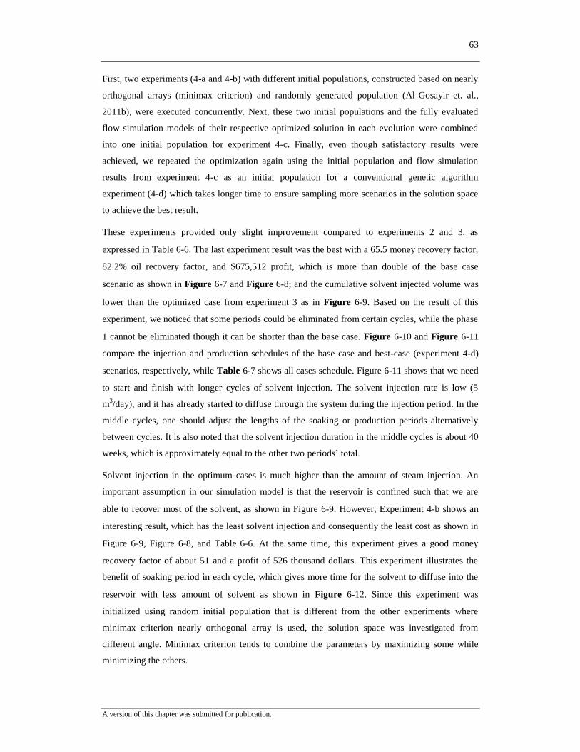
63
A version of this chapter was submitted for publication.
First, two experiments (4-a and 4-b) with different initial populations, constructed based on nearly
orthogonal arrays (minimax criterion) and randomly generated population (Al-Gosayir et. al.,
2011b), were executed concurrently. Next, these two initial populations and the fully evaluated
flow simulation models of their respective optimized solution in each evolution were combined
into one initial population for experiment 4-c. Finally, even though satisfactory results were
achieved, we repeated the optimization again using the initial population and flow simulation
results from experiment 4-c as an initial population for a conventional genetic algorithm
experiment (4-d) which takes longer time to ensure sampling more scenarios in the solution space
to achieve the best result.
These experiments provided only slight improvement compared to experiments 2 and 3, as
expressed in Table 6-6. The last experiment result was the best with a 65.5 money recovery factor,
82.2% oil recovery factor, and $675,512 profit, which is more than double of the base case
scenario as shown in Figure 6-7 and Figure 6-8; and the cumulative solvent injected volume was
lower than the optimized case from experiment 3 as in Figure 6-9. Based on the result of this
experiment, we noticed that some periods could be eliminated from certain cycles, while the phase
1 cannot be eliminated though it can be shorter than the base case. Figure 6-10 and Figure 6-11
compare the injection and production schedules of the base case and best-case (experiment 4-d)
scenarios, respectively, while Table 6-7 shows all cases schedule. Figure 6-11 shows that we need
to start and finish with longer cycles of solvent injection. The solvent injection rate is low (5
m3/day), and it has already started to diffuse through the system during the injection period. In the
middle cycles, one should adjust the lengths of the soaking or production periods alternatively
between cycles. It is also noted that the solvent injection duration in the middle cycles is about 40
weeks, which is approximately equal to the other two periods’total.
Solvent injection in the optimum cases is much higher than the amount of steam injection. An
important assumption in our simulation model is that the reservoir is confined such that we are
able to recover most of the solvent, as shown in Figure 6-9. However, Experiment 4-b shows an
interesting result, which has the least solvent injection and consequently the least cost as shown in
Figure 6-9, Figure 6-8, and Table 6-6. At the same time, this experiment gives a good money
recovery factor of about 51 and a profit of 526 thousand dollars. This experiment illustrates the
benefit of soaking period in each cycle, which gives more time for the solvent to diffuse into the
reservoir with less amount of solvent as shown in Figure 6-12. Since this experiment was
initialized using random initial population that is different from the other experiments where
minimax criterion nearly orthogonal array is used, the solution space was investigated from
different angle. Minimax criterion tends to combine the parameters by maximizing some while
minimizing the others.

64
A version of this chapter was submitted for publication.
Conclusions and remarks
Despite the challenge of optimizing the injection time and cycles of the SOS-FR process using
hybrid genetic algorithm, the outcome was very promising and better results than the benchmark
case were achieved. The money recovery factor and the profit were doubled and about 30% oil
recovery increase was obtained. The results suggest that steam heating period should be decreased,
while the solvent injection time to be increased without eliminating the necessity of having solvent
soaking or production periods. Handling such complex process optimization is a challenge, which
could be overcome by implementing a hybrid optimization scheme that incorporates a detailed
sensitivity analysis with experimental design methods for initial population construction, followed
by a global optimization scheme of genetic algorithm, whose convergence efficiency was
improved with the use of response surfaces. In addition, the accuracy of the proxy model was
further enhanced with a periodic updating step in which additional flow simulation results using
the most optimal case were used to re-calibrate the response surface at each evolution.
Furthermore, we noticed that hybrid genetic algorithm is a useful tool designing the operating
strategy of a complex recovery process by optimizing the time required for each phase of the SOS-
FR method.
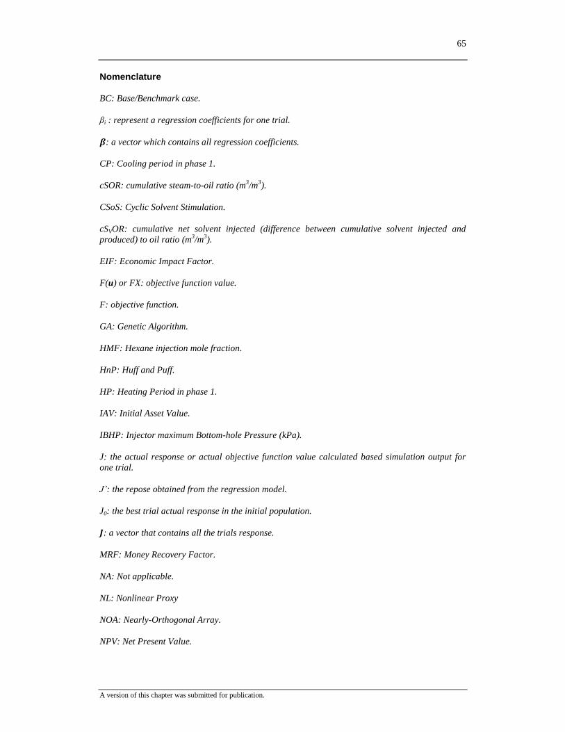
65
A version of this chapter was submitted for publication.
Nomenclature
BC: Base/Benchmark case.
βi : represent a regression coefficients for one trial.
: a vector which contains all regression coefficients.
CP: Cooling period in phase 1.
cSOR: cumulative steam-to-oil ratio (m3/m
3).
CSoS: Cyclic Solvent Stimulation.
cSVOR: cumulative net solvent injected (difference between cumulative solvent injected and
produced) to oil ratio (m3/m
3).
EIF: Economic Impact Factor.
F(u) or FX: objective function value.
F: objective function.
GA: Genetic Algorithm.
HMF: Hexane injection mole fraction.
HnP: Huff and Puff.
HP: Heating Period in phase 1.
IAV: Initial Asset Value.
IBHP: Injector maximum Bottom-hole Pressure (kPa).
J: the actual response or actual objective function value calculated based simulation output for
one trial.
J’: the repose obtained from the regression model.
J0: the best trial actual response in the initial population.
: a vector that contains all the trials response.
MRF: Money Recovery Factor.
NA: Not applicable.
NL: Nonlinear Proxy
NOA: Nearly-Orthogonal Array.
NPV: Net Present Value.

66
A version of this chapter was submitted for publication.
OA: Orthogonal Array.
PBHP: Producer minimum Bottom-hole Pressure.
PP: Production period in each cycle.
RF: Recovery Factor.
RP: Recovery phase 3.
SAGD: Steam Assisted Gravity Drainage thermal recovery process.
SIP: Solvent Injection period in each cycle.
SOP: Solvent Soaking period in each cycle.
SOS-FR: Steam-Over-Solvent for Fractured Reservoirs.
STOIIP: Stock Tank Oil Initially In Place.
u: a (1*n) vector which contains the optimization variables for a trial.
ui : represent an optimization variable for one trial.
: a matrix with all u’s.
USD United States Dollar.
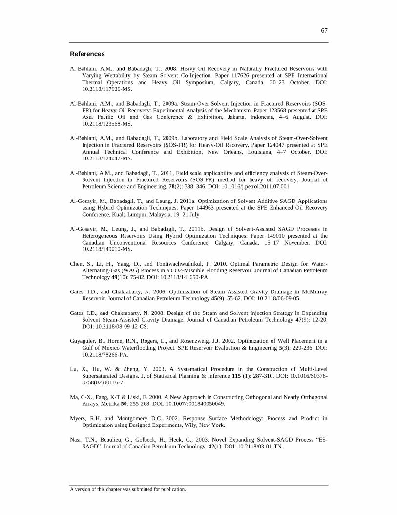
67
A version of this chapter was submitted for publication.
References
Al-Bahlani, A.M., and Babadagli, T., 2008. Heavy-Oil Recovery in Naturally Fractured Reservoirs with
Varying Wettability by Steam Solvent Co-Injection. Paper 117626 presented at SPE International
Thermal Operations and Heavy Oil Symposium, Calgary, Canada, 20–23 October. DOI:
10.2118/117626-MS.
Al-Bahlani, A.M., and Babadagli, T., 2009a. Steam-Over-Solvent Injection in Fractured Reservoirs (SOS-
FR) for Heavy-Oil Recovery: Experimental Analysis of the Mechanism. Paper 123568 presented at SPE
Asia Pacific Oil and Gas Conference & Exhibition, Jakarta, Indonesia, 4–6 August. DOI:
10.2118/123568-MS.
Al-Bahlani, A.M., and Babadagli, T., 2009b. Laboratory and Field Scale Analysis of Steam-Over-Solvent
Injection in Fractured Reservoirs (SOS-FR) for Heavy-Oil Recovery. Paper 124047 presented at SPE
Annual Technical Conference and Exhibition, New Orleans, Louisiana, 4–7 October. DOI:
10.2118/124047-MS.
Al-Bahlani, A.M., and Babadagli, T., 2011, Fieldscaleapplicabilityandefficiency analysis of Steam-Over-
Solvent Injection in Fractured Reservoirs (SOS-FR) method for heavy oil recovery. Journal of
Petroleum Science and Engineering, 78(2): 338–346. DOI: 10.1016/j.petrol.2011.07.001
Al-Gosayir, M., Babadagli, T., and Leung, J. 2011a. Optimization of Solvent Additive SAGD Applications
using Hybrid Optimization Techniques. Paper 144963 presented at the SPE Enhanced Oil Recovery
Conference, Kuala Lumpur, Malaysia, 19–21 July.
Al-Gosayir, M., Leung, J., and Babadagli, T., 2011b. Design of Solvent-Assisted SAGD Processes in
Heterogeneous Reservoirs Using Hybrid Optimization Techniques. Paper 149010 presented at the
Canadian Unconventional Resources Conference, Calgary, Canada, 15–17 November. DOI:
10.2118/149010-MS.
Chen, S., Li, H., Yang, D., and Tontiwachwuthikul, P. 2010. Optimal Parametric Design for Water-
Alternating-Gas (WAG) Process in a CO2-Miscible Flooding Reservoir. Journal of Canadian Petroleum
Technology 49(10): 75-82. DOI: 10.2118/141650-PA
Gates, I.D., and Chakrabarty, N. 2006. Optimization of Steam Assisted Gravity Drainage in McMurray
Reservoir. Journal of Canadian Petroleum Technology 45(9): 55-62. DOI: 10.2118/06-09-05.
Gates, I.D., and Chakrabarty, N. 2008. Design of the Steam and Solvent Injection Strategy in Expanding
Solvent Steam-Assisted Gravity Drainage. Journal of Canadian Petroleum Technology 47(9): 12-20.
DOI: 10.2118/08-09-12-CS.
Guyaguler, B., Horne, R.N., Rogers, L., and Rosenzweig, J.J. 2002. Optimization of Well Placement in a
Gulf of Mexico Waterflooding Project. SPE Reservoir Evaluation & Engineering 5(3): 229-236. DOI:
10.2118/78266-PA.
Lu, X., Hu, W. & Zheng, Y. 2003. A Systematical Procedure in the Construction of Multi-Level
Supersaturated Designs. J. of Statistical Planning & Inference 115 (1): 287-310. DOI: 10.1016/S0378-
3758(02)00116-7.
Ma, C-X., Fang, K-T & Liski, E. 2000. A New Approach in Constructing Orthogonal and Nearly Orthogonal
Arrays. Metrika 50: 255-268. DOI: 10.1007/s001840050049.
Myers, R.H. and Montgomery D.C. 2002. Response Surface Methodology: Process and Product in
Optimization using Designed Experiments, Wily, New York.
Nasr, T.N., Beaulieu, G., Golbeck, H., Heck, G., 2003. Novel Expanding Solvent-SAGD Process “ES-
SAGD”. Journal of Canadian Petroleum Technology. 42(1). DOI: 10.2118/03-01-TN.

68
A version of this chapter was submitted for publication.
Peterson, J., Riva, D., Edmunds, N., and Solanki, S. 2010. The Application of Solvent-Additive SAGD
Processes in Reservoirs With Associated Basal Water. Paper 137833 presented at Canadian
Unconventional Resources and International Petroleum Conference, Calgary, Alberta, Canada, 19-21
October. DOI: 10.2118/137833-MS.
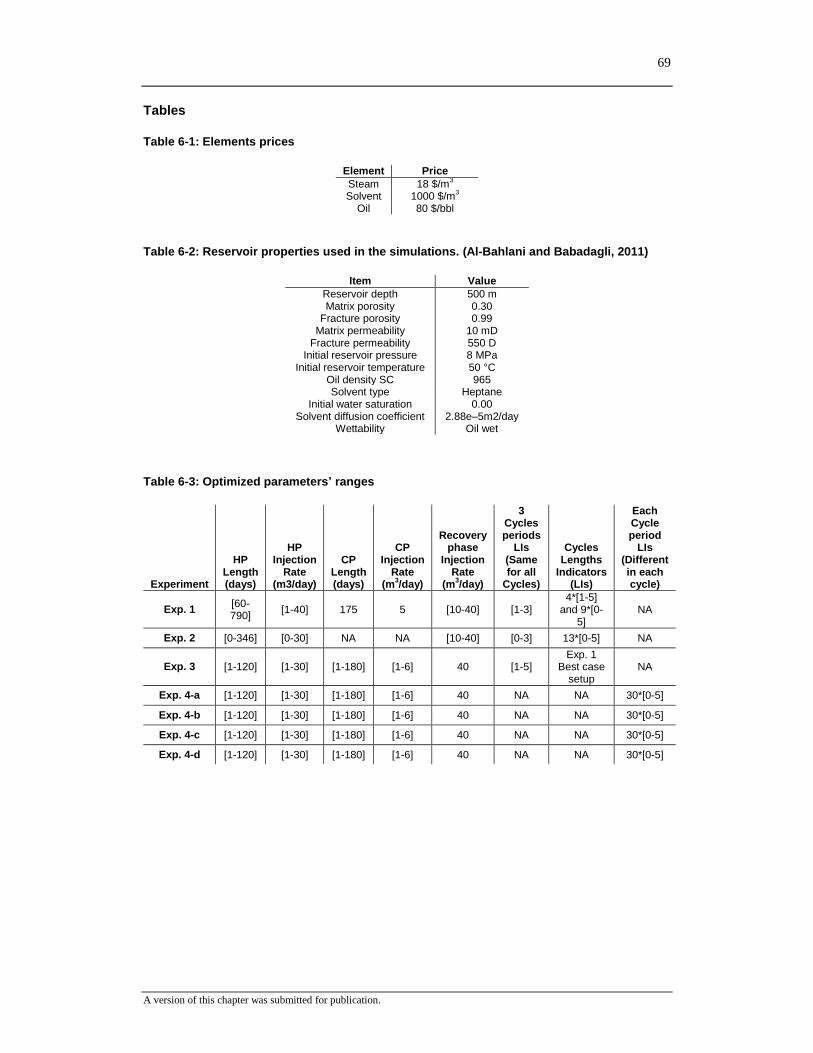
69
A version of this chapter was submitted for publication.
Tables
Table 6-1: Elements prices
Element Price
Steam 18 $/m3
Solvent 1000 $/m3
Oil 80 $/bbl
Table 6-2: Reservoir properties used in the simulations. (Al-Bahlani and Babadagli, 2011)
Item Value Reservoir depth 500 m Matrix porosity 0.30
Fracture porosity 0.99 Matrix permeability 10 mD
Fracture permeability 550 D Initial reservoir pressure 8 MPa
Initial reservoir temperature 50 °C Oil density SC 965 Solvent type Heptane
Initial water saturation 0.00 Solvent diffusion coefficient 2.88e–5m2/day
Wettability Oil wet
Table 6-3: Optimized parameters’ ranges
Experiment
HP Length (days)
HP Injection
Rate (m3/day)
CP Length (days)
CP Injection
Rate (m
3/day)
Recovery phase
Injection Rate
(m3/day)
3 Cycles periods
LIs (Same for all
Cycles)
Cycles Lengths
Indicators (LIs)
Each Cycle period
LIs (Different in each cycle)
Exp. 1 [60-790]
[1-40] 175 5 [10-40] [1-3] 4*[1-5]
and 9*[0-5]
NA
Exp. 2 [0-346] [0-30] NA NA [10-40] [0-3] 13*[0-5] NA
Exp. 3 [1-120] [1-30] [1-180] [1-6] 40 [1-5] Exp. 1
Best case setup
NA
Exp. 4-a [1-120] [1-30] [1-180] [1-6] 40 NA NA 30*[0-5]
Exp. 4-b [1-120] [1-30] [1-180] [1-6] 40 NA NA 30*[0-5]
Exp. 4-c [1-120] [1-30] [1-180] [1-6] 40 NA NA 30*[0-5]
Exp. 4-d [1-120] [1-30] [1-180] [1-6] 40 NA NA 30*[0-5]
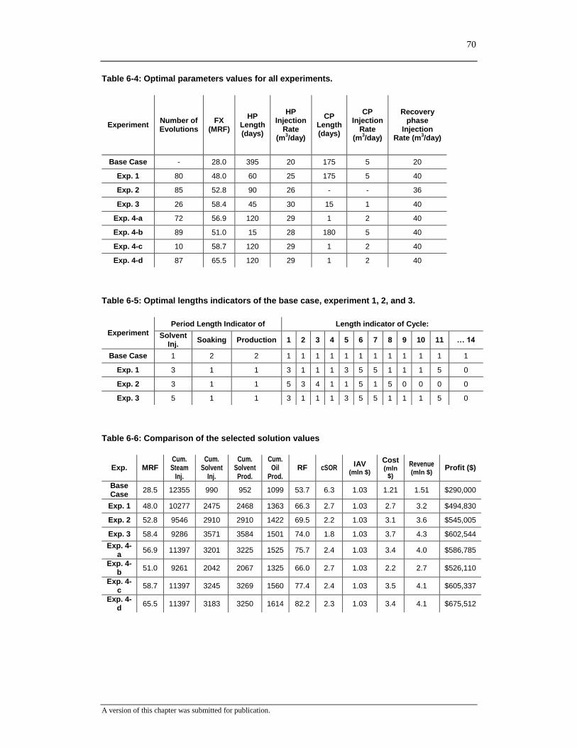
70
A version of this chapter was submitted for publication.
Table 6-4: Optimal parameters values for all experiments.
Experiment Number of Evolutions
FX (MRF)
HP Length (days)
HP Injection
Rate (m
3/day)
CP Length (days)
CP Injection
Rate (m
3/day)
Recovery phase
Injection Rate (m
3/day)
Base Case - 28.0 395 20 175 5 20
Exp. 1 80 48.0 60 25 175 5 40
Exp. 2 85 52.8 90 26 - - 36
Exp. 3 26 58.4 45 30 15 1 40
Exp. 4-a 72 56.9 120 29 1 2 40
Exp. 4-b 89 51.0 15 28 180 5 40
Exp. 4-c 10 58.7 120 29 1 2 40
Exp. 4-d 87 65.5 120 29 1 2 40
Table 6-5: Optimal lengths indicators of the base case, experiment 1, 2, and 3.
Experiment
Period Length Indicator of Length indicator of Cycle:
Solvent Inj.
Soaking Production 1 2 3 4 5 6 7 8 9 10 11 … 14
Base Case 1 2 2 1 1 1 1 1 1 1 1 1 1 1 1
Exp. 1 3 1 1 3 1 1 1 3 5 5 1 1 1 5 0
Exp. 2 3 1 1 5 3 4 1 1 5 1 5 0 0 0 0
Exp. 3 5 1 1 3 1 1 1 3 5 5 1 1 1 5 0
Table 6-6: Comparison of the selected solution values
Exp. MRF Cum. Steam
Inj.
Cum. Solvent
Inj.
Cum. Solvent Prod.
Cum. Oil
Prod. RF cSOR
IAV (mln $)
Cost (mln
$)
Revenue (mln $)
Profit ($)
Base Case
28.5 12355 990 952 1099 53.7 6.3 1.03 1.21 1.51 $290,000
Exp. 1 48.0 10277 2475 2468 1363 66.3 2.7 1.03 2.7 3.2 $494,830
Exp. 2 52.8 9546 2910 2910 1422 69.5 2.2 1.03 3.1 3.6 $545,005
Exp. 3 58.4 9286 3571 3584 1501 74.0 1.8 1.03 3.7 4.3 $602,544
Exp. 4-a
56.9 11397 3201 3225 1525 75.7 2.4 1.03 3.4 4.0 $586,785
Exp. 4-b
51.0 9261 2042 2067 1325 66.0 2.7 1.03 2.2 2.7 $526,110
Exp. 4-c
58.7 11397 3245 3269 1560 77.4 2.4 1.03 3.5 4.1 $605,337
Exp. 4-d
65.5 11397 3183 3250 1614 82.2 2.3 1.03 3.4 4.1 $675,512

71
A version of this chapter was submitted for publication.
Table 6-7: Experiments huff-and-puff phases lengths in days
Cycle 1 Cycle 2 Cycle 3 Cycle 4 Cycle 5 Cycle 6
Exp. SIP SOP PP SIP SOP PP SIP SOP PP SIP SOP PP SIP SOP PP SIP SOP PP
BC 7 14 14 7 14 14 7 14 14 7 14 14 7 14 14 7 14 14
1 55 18 18 18 6 6 18 6 6 18 6 6 55 18 18 92 31 31
2 116 39 39 70 23 23 93 31 31 23 8 8 23 8 8 116 39 39
3 79 16 16 26 5 5 26 5 5 26 5 5 79 16 16 132 26 26
4-a 142 14 0 43 43 14 57 0 28 71 14 0 28 43 0 71 57 28
4-b 48 36 0 48 60 24 48 60 0 60 36 36 36 12 48 24 24 0
4-c 138 14 0 41 41 14 55 0 28 69 14 0 69 41 0 69 55 28
4-d 159 16 0 32 64 16 64 0 16 80 16 0 80 48 0 16 64 32
Cycle 7 Cycle 8 Cycle 9 Cycle 10 Cycle 11 … Cycle 14
Exp. SIP SOP PP SIP SOP PP SIP SOP PP SIP SOP PP SIP SOP PP SIP SOP PP
BC 7 14 14 7 14 14 7 14 14 7 14 14 7 14 14 7 14 14
1 92 31 31 18 6 6 18 6 6 18 6 6 92 31 31
2 23 8 8 116 39 39
3 132 26 26 26 5 5 26 5 5 26 5 5 132 26 26
4-a 57 0 14 57 28 0 71 43 14
4-b 60 24 0 60 48 0 24 48 0
4-c 55 14 14 124 41 14
4-d 16 0 16 159 48 0
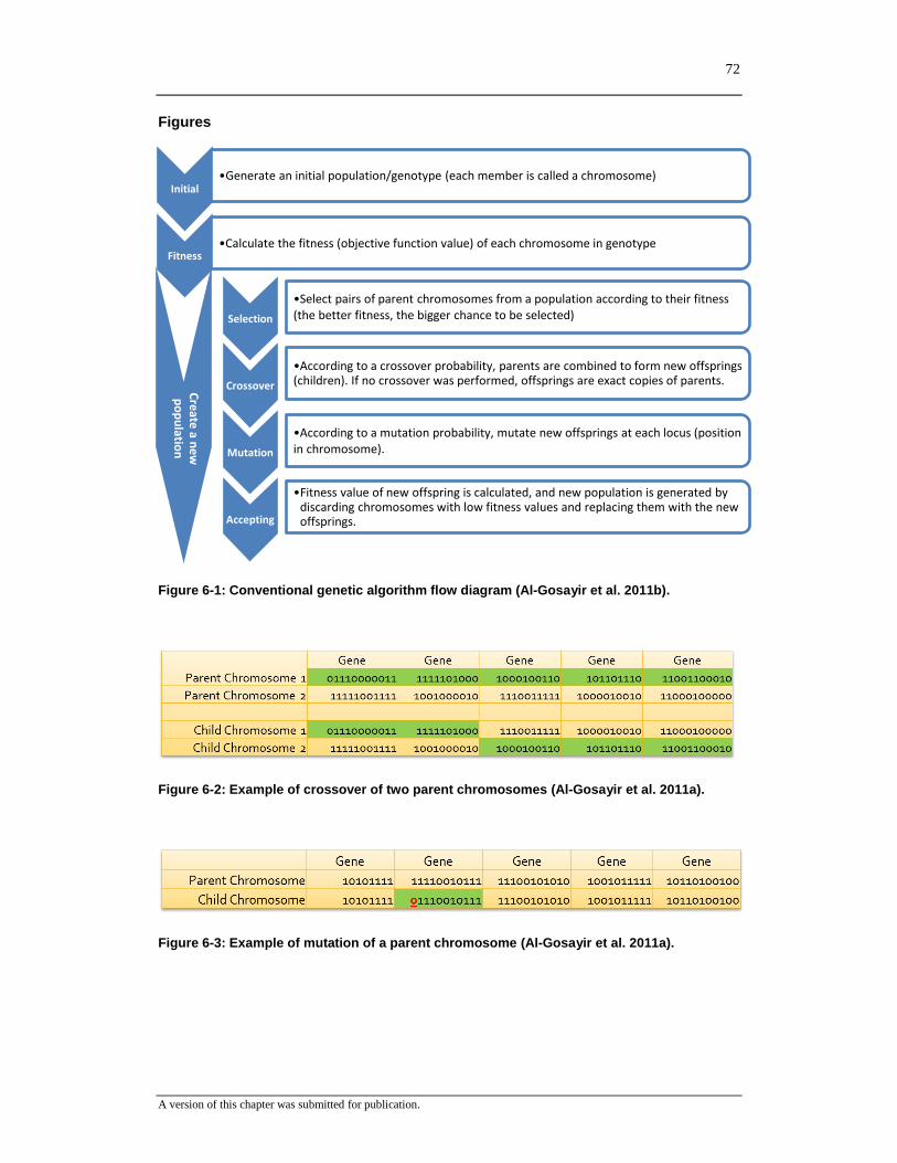
72
A version of this chapter was submitted for publication.
Figures
Figure 6-1: Conventional genetic algorithm flow diagram (Al-Gosayir et al. 2011b).
Figure 6-2: Example of crossover of two parent chromosomes (Al-Gosayir et al. 2011a).
Figure 6-3: Example of mutation of a parent chromosome (Al-Gosayir et al. 2011a).
Initial •Generate an initial population/genotype (each member is called a chromosome)
Fitness •Calculate the fitness (objective function value) of each chromosome in genotype
Selection
•Select pairs of parent chromosomes from a population according to their fitness (the better fitness, the bigger chance to be selected)
Crossover
•According to a crossover probability, parents are combined to form new offsprings (children). If no crossover was performed, offsprings are exact copies of parents.
Mutation
•According to a mutation probability, mutate new offsprings at each locus (position in chromosome).
Accepting
•Fitness value of new offspring is calculated, and new population is generated by discarding chromosomes with low fitness values and replacing them with the new offsprings.
Cre
ate a n
ew
p
op
ulatio
n
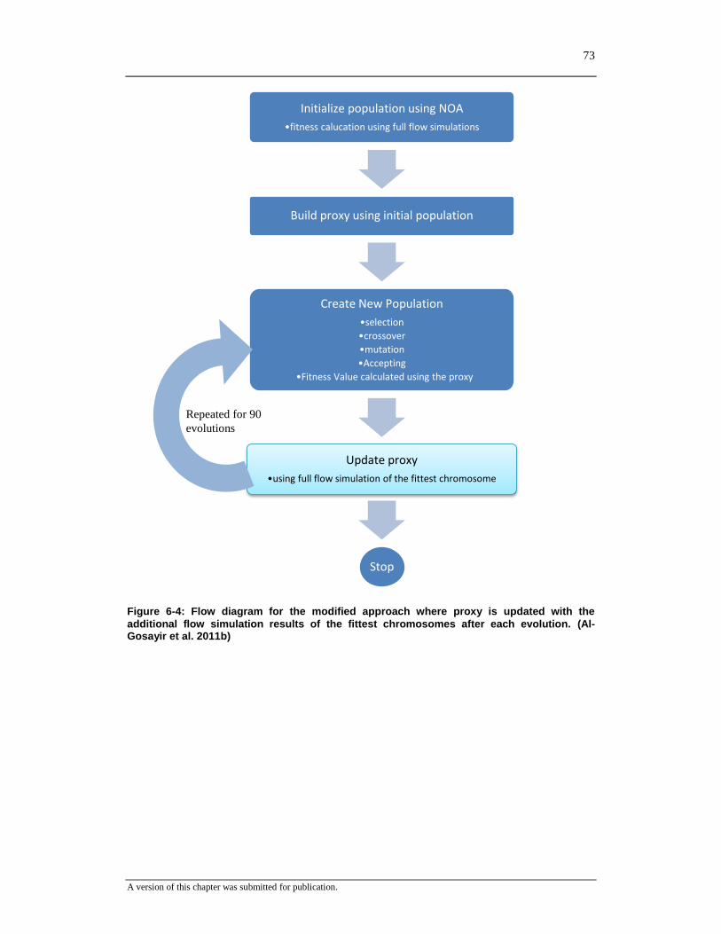
73
A version of this chapter was submitted for publication.
Figure 6-4: Flow diagram for the modified approach where proxy is updated with the
additional flow simulation results of the fittest chromosomes after each evolution. (Al-Gosayir et al. 2011b)
Initialize population using NOA
•fitness calucation using full flow simulations
Build proxy using initial population
Create New Population
•selection
•crossover
•mutation
•Accepting
•Fitness Value calculated using the proxy
Update proxy
•using full flow simulation of the fittest chromosome
Stop
Repeated for 90
evolutions
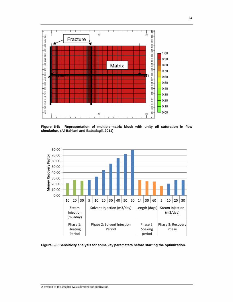
74
A version of this chapter was submitted for publication.
Figure 6-5: Representation of multiple-matrix block with unity oil saturation in flow
simulation. (Al-Bahlani and Babadagli, 2011)
Figure 6-6: Sensitivity analysis for some key parameters before starting the optimization.
0.00
10.00
20.00
30.00
40.00
50.00
60.00
70.00
80.00
10 20 30 5 10 20 30 40 50 60 14 30 60 5 10 20 30
SteamInjection(m3/day)
Solvent Injection (m3/day) Length (days) Steam Injection(m3/day)
Phase 1:HeatingPeriod
Phase 2: Solvent InjectionPeriod
Phase 2:Soakingperiod
Phase 3: RecoveryPhase
Mo
ne
y R
eco
very
Fac
tor
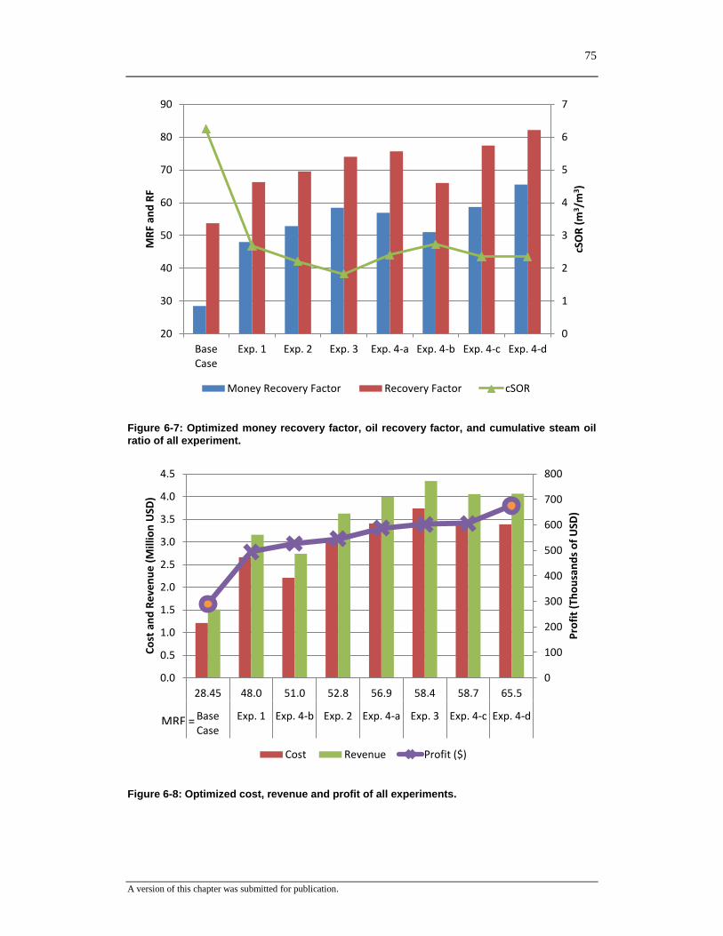
75
A version of this chapter was submitted for publication.
Figure 6-7: Optimized money recovery factor, oil recovery factor, and cumulative steam oil
ratio of all experiment.
Figure 6-8: Optimized cost, revenue and profit of all experiments.
0
1
2
3
4
5
6
7
20
30
40
50
60
70
80
90
BaseCase
Exp. 1 Exp. 2 Exp. 3 Exp. 4-a Exp. 4-b Exp. 4-c Exp. 4-d
cSO
R (
m3/m
3 )
MR
F an
d R
F
Money Recovery Factor Recovery Factor cSOR
0
100
200
300
400
500
600
700
800
0.0
0.5
1.0
1.5
2.0
2.5
3.0
3.5
4.0
4.5
28.45 48.0 51.0 52.8 56.9 58.4 58.7 65.5
BaseCase
Exp. 1 Exp. 4-b Exp. 2 Exp. 4-a Exp. 3 Exp. 4-c Exp. 4-d
Pro
fit
(Th
ou
san
ds
of
USD
)
Co
st a
nd
Re
ven
ue
(M
illio
n U
SD)
Cost Revenue Profit ($)
MRF =
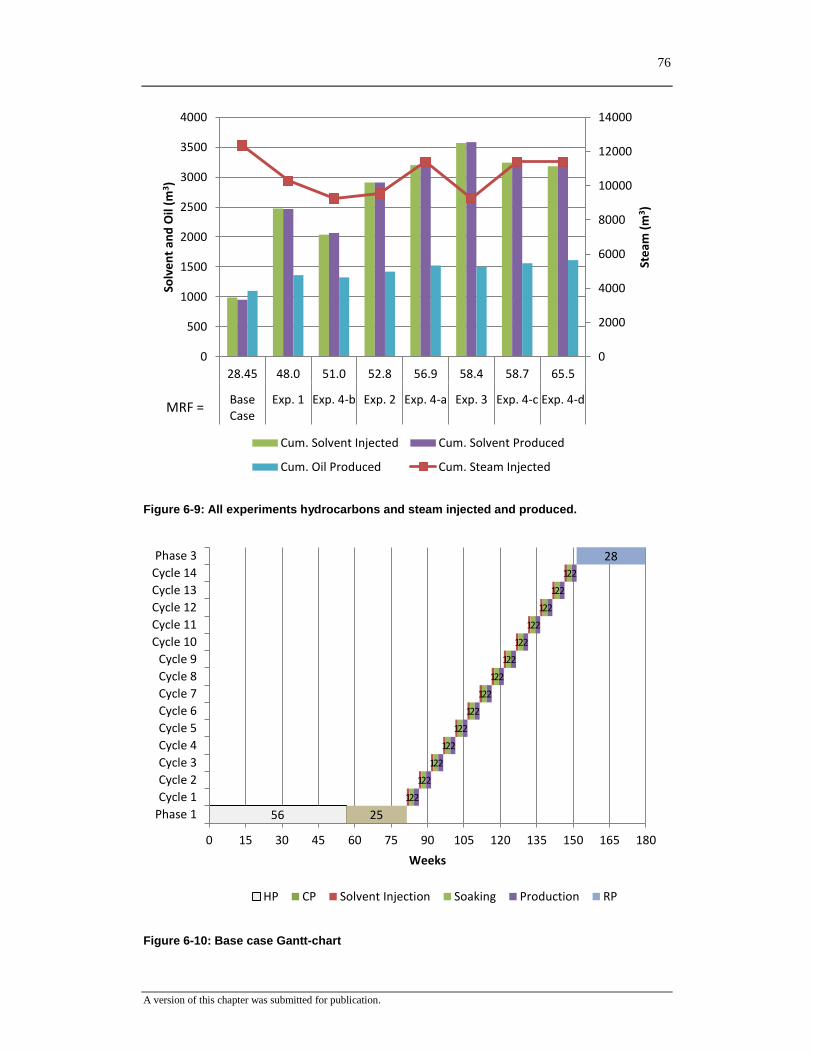
76
A version of this chapter was submitted for publication.
Figure 6-9: All experiments hydrocarbons and steam injected and produced.
Figure 6-10: Base case Gantt-chart
0
2000
4000
6000
8000
10000
12000
14000
0
500
1000
1500
2000
2500
3000
3500
4000
28.45 48.0 51.0 52.8 56.9 58.4 58.7 65.5
BaseCase
Exp. 1 Exp. 4-b Exp. 2 Exp. 4-a Exp. 3 Exp. 4-c Exp. 4-d
Ste
am (
m3 )
Solv
en
t an
d O
il (m
3)
Cum. Solvent Injected Cum. Solvent Produced
Cum. Oil Produced Cum. Steam Injected
MRF =
56 25
1
1
1
1
1
1
1
1
1
1
1
1
1
1
2
2
2
2
2
2
2
2
2
2
2
2
2
2
2
2
2
2
2
2
2
2
2
2
2
2
2
2
28
0 15 30 45 60 75 90 105 120 135 150 165 180
Phase 1
Cycle 1
Cycle 2
Cycle 3
Cycle 4
Cycle 5
Cycle 6
Cycle 7
Cycle 8
Cycle 9
Cycle 10
Cycle 11
Cycle 12
Cycle 13
Cycle 14
Phase 3
Weeks
HP CP Solvent Injection Soaking Production RP
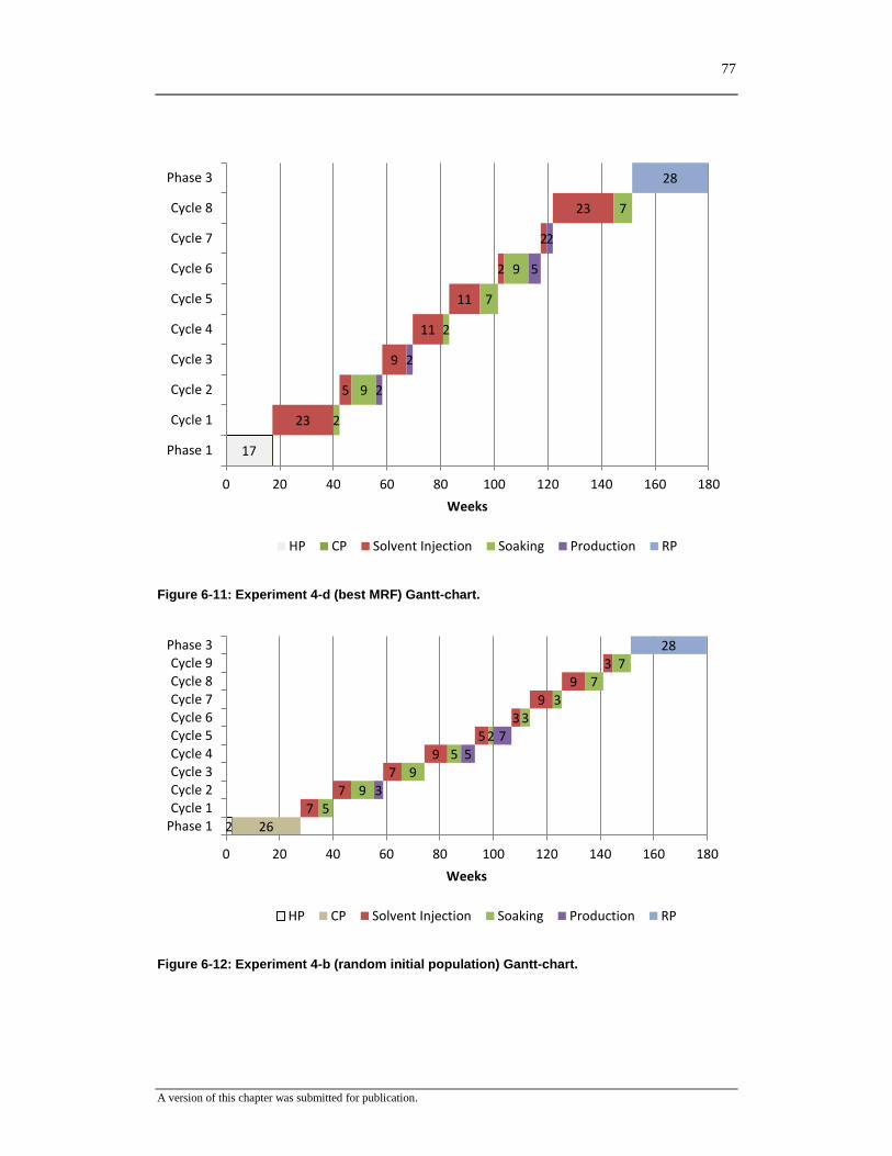
77
A version of this chapter was submitted for publication.
Figure 6-11: Experiment 4-d (best MRF) Gantt-chart.
Figure 6-12: Experiment 4-b (random initial population) Gantt-chart.
17
23
5
9
11
11
2
2
23
2
9
2
7
9
7
2
2
5
2
28
0 20 40 60 80 100 120 140 160 180
Phase 1
Cycle 1
Cycle 2
Cycle 3
Cycle 4
Cycle 5
Cycle 6
Cycle 7
Cycle 8
Phase 3
Weeks
HP CP Solvent Injection Soaking Production RP
2 26 7
7 7
9 5
3 9
9 3
5 9
9 5
2 3
3 7
7
3
5 7
28
0 20 40 60 80 100 120 140 160 180
Phase 1Cycle 1Cycle 2Cycle 3Cycle 4Cycle 5Cycle 6Cycle 7Cycle 8Cycle 9
Phase 3
Weeks
HP CP Solvent Injection Soaking Production RP
78
Chapter 7: Contributions
There are several major contributions gained out of this thesis as listed below:
1. A hybrid optimization strategy, integrating elements of experimental design (orthogonal
arrays) and response surface proxy into a global genetic algorithm optimization
workflow, was developed. The adopted proxy provided a saving of 95% computational
time, while the use of orthogonal arrays (with minimax criterion) was shown to improve
thealgorithm’sconvergencebehaviorinseekingtheoptimalsolution.
2. It was observed that non-linear response surface proxy can potentially give a more
accurate representation of the true objective function value, but it also tends to over-shoot
during extrapolations. Therefore, a periodic updating scheme was proposed and
implemented. The success of this step was illustrated by the improved predictability of
the objective function and minimal increase in computational time.
3. The proposed technique was applied to construct optimal designs for three different
heavy oil recovery processes using steam and solvent. In particular, the computational
efficiency of the technique allows optimization to be carried out successfully for
heterogeneous reservoirs. These case studies illustrated that the hybrid optimization
framework is a useful tool for designing complex recovery processes and increasing the
profit.
79
Appendix 1: JGAP initializer code
package mmm.ga.tests;
import java.io.BufferedReader;
import java.io.FileReader;
import java.io.IOException;
import java.util.List;
import java.util.Vector;
import mmm.ga.MyGenericChromosome;
import org.jgap.*;
import org.jgap.audit.ChainedMonitors;
import org.jgap.audit.EvolutionMonitor;
import org.jgap.audit.FitnessImprovementMonitor;
import org.jgap.audit.IEvolutionMonitor;
import org.jgap.audit.TimedMonitor;
import org.jgap.impl.*;
import Jama.Matrix;
public abstract class GenericRunner {
int evolutions;
Genotype population;
IEvolutionMonitor monitor;
FitnessFunction objectiveFunction;
public GenericRunner(String runTitle, int evolutions, int
a_sizeOfPopulation, FitnessFunction objectiveFunction) throws Exception {
System.out.println(runTitle);
this.evolutions = evolutions;
this.objectiveFunction = objectiveFunction;
// Start with a DefaultConfiguration, which comes setup with the
// most common settings.
// -------------------------------------------------------------
Configuration gaConf = new DefaultConfiguration();
// Care that the fittest individual of the current population is
// always taken to the next generation.
// -------------------------------------------------------------
boolean preservFittestIndividual = false;
gaConf.setPreservFittestIndividual(preservFittestIndividual);
System.out.println("setPreservFittestIndividual\t"
+ preservFittestIndividual);
// Set the fitness function we want to use, which is our
// ------------------------------------------------------------
gaConf.setFitnessFunction(this.objectiveFunction);
boolean alwaysCaculateFitness = true;
System.out.println("alwaysCaculateFitness\t" +
alwaysCaculateFitness);
gaConf.setAlwaysCaculateFitness(alwaysCaculateFitness);
double crossoverRatePercentage = 0.35d;
int mutationRate = 3;
gaConf.getGeneticOperators().clear();
gaConf.addGeneticOperator(new CrossoverOperator(gaConf,
crossoverRatePercentage));
gaConf.addGeneticOperator(new MutationOperator(gaConf,
mutationRate));
System.out.println("Crossover rate\t" + crossoverRatePercentage);
80
System.out.println("Mutation rate\t" + mutationRate);
boolean allowDoubllette = false;
double originalRate = 0.9;
BestChromosomesSelector s = (BestChromosomesSelector) gaConf
.getNaturalSelector();
s.setDoubletteChromosomesAllowed(allowDoubllette);
s.setOriginalRate(originalRate);
System.out.println("allowDoubllette\t" + allowDoubllette);
System.out.println("originalRate\t" + originalRate);
List monitors = new Vector();
monitors.add(new TimedMonitor(6));
monitors.add(new FitnessImprovementMonitor(1, 3, 5.0d));
monitors.add(new EvolutionMonitor());
monitor = new ChainedMonitors(monitors, 3);
System.out.println("Monitors on.");
IChromosome sampleChromosome = getSampleChromosome(gaConf);
gaConf.setSampleChromosome(sampleChromosome);
System.out.println("Sample Genes:");
for (Gene gene : sampleChromosome.getGenes()) {
System.out.println(gene);
}
// Finally, we need to tell the Configuration object how many
// Chromosomes we want in our population. The more Chromosomes,
// the larger the number of potential solutions (which is good
// for finding the answer), but the longer it will take to evolve
// the population each round.
gaConf.setPopulationSize(a_sizeOfPopulation);
System.out.println("Population Size\t" + a_sizeOfPopulation);
// Create random initial population of Chromosomes.
System.out.println("Random Initial Population Generated");
population = Genotype.randomInitialGenotype(gaConf);
//population = new
Genotype(gaConf,NoaArrayImporter.getInitialNAOPopulation(gaConf, 0, 0));
}
protected IChromosome getSampleChromosome(Configuration gaConf)
throws InvalidConfigurationException {
// Now we need to tell the Configuration object how we want our
// Chromosomes to be setup. We do that by actually creating a
// sample Chromosome and then setting it on the Configuration
// object.
int chromeSize = 19; //
Gene[] sampleGenes = new Gene[chromeSize];
//Heating Phase length: multiple integer [60-790] days with 30 days
level length
sampleGenes[0] = new MutipleIntegerGene(gaConf, 60, 790, 30);
//Heating Phase steam injection rate
sampleGenes[1] = new DoubleGene(gaConf, 10, 40);
//Cycles lengths indicators
sampleGenes[2] = new IntegerGene(gaConf,1,5);
sampleGenes[3] = new IntegerGene(gaConf,1,5);
sampleGenes[4] = new IntegerGene(gaConf,1,5);
sampleGenes[5] = new IntegerGene(gaConf,1,5);
sampleGenes[6] = new IntegerGene(gaConf,0,5);
sampleGenes[7] = new IntegerGene(gaConf,0,5);
sampleGenes[8] = new IntegerGene(gaConf,0,5);
sampleGenes[9] = new IntegerGene(gaConf,0,5);
sampleGenes[10] = new IntegerGene(gaConf,0,5);
sampleGenes[11] = new IntegerGene(gaConf,0,5);
81
sampleGenes[12] = new IntegerGene(gaConf,0,5);
sampleGenes[13] = new IntegerGene(gaConf,0,5);
sampleGenes[14] = new IntegerGene(gaConf,0,5);
//sampleGenes[15] = new IntegerGene(gaConf,0,5);
//Cycles periods (3 periods one of them soaking)
sampleGenes[15] = new IntegerGene(gaConf,1,3);
sampleGenes[16] = new IntegerGene(gaConf,1,3);
sampleGenes[17] = new IntegerGene(gaConf,1,3);
//Recovery Phase steam injection rate
sampleGenes[18] = new DoubleGene(gaConf, 10, 40);
IChromosome sampleChromosome = new MyGenericChromosome(gaConf,
chromeSize);
sampleChromosome.setGenes(sampleGenes);
return sampleChromosome;
}
package mmm.ga.tests;
import java.io.IOException;
import java.util.List;
import mmm.cmgAgents.*;
import mmm.ga.MyGenericChromosome;
import mmm.ga.objectiveFunctions.NonLinearProxyObjectiveFunction;
import mmm.sosfr.SosFrPreprossor2;
import org.jgap.*;
import org.jgap.impl.DoubleGene;
import org.jgap.impl.IntegerGene;
import org.jgap.impl.MutipleIntegerGene;
public class ProxyEvolutionFittestRun3 extends GenericRunner {
public ProxyEvolutionFittestRun3(String runTitle, int evolutions, int
a_sizeOfPopulation, FitnessFunction objectiveFunction) throws Exception {
super(runTitle, evolutions, a_sizeOfPopulation, objectiveFunction);
Configuration gaConf = super.population.getConfiguration();
//Override the random population with an old population to avoid
re-running the simulations
population = new
Genotype(gaConf,getInitialNAOPopulation(gaConf,"ex3_good_62cases.txt"));
}
@Override
public void run() throws Exception {
System.out.println("Evolution Start\t" + evolutions +
"\tevoluions");
System.out.println();
System.out
.println("Location\tEvolution\tFX\tmaxEN\t");
System.out.println("FileInfo\tp1l\tp1injRate\tRPInjRate\tAllCyclesLength\tC
yclesCount\tcp1\tcp2\tcp3\tCyclesLengths");
System.out.println("ObjValues\tmoneyRecoveryFactor\tCumSteamInj\tCumSolInj\
tCumSolProd\tCumOilProd\tRF\tcSOR\tiav\tcost\trevenue\tgrossProfit");
long startTime = System.currentTimeMillis();
NonLinearProxyObjectiveFunction obj =
(NonLinearProxyObjectiveFunction)objectiveFunction;
for (int i = 0; i < evolutions; i++) {
82
for (IChromosome c1 :
population.getPopulation().getChromosomes()) {
MyGenericChromosome c = (MyGenericChromosome) c1;
System.out.println("****PC*****\t" + i + "\t"
+ c.getFitnessValue() + "\t\t" + c);
}
if (!uniqueChromosomes(population.getPopulation())) {
System.out.println("Invalid state in generation\t" +
i);
}
if (monitor != null) {
List<String> messages = population.evolve(monitor);
if (messages.size() > 0) {
for (String msg : messages) {
System.out.println("Monitor:\t" + i +
msg);
}
}
} else {
population.evolve();
}
MyGenericChromosome fittest = (MyGenericChromosome)
population
.getFittestChromosome();
System.out.println("Currently fittest Chromosome\t" + i +
"\t"
+ fittest.getFitnessValue() + "\t" +
fittest);
long simStartTime = System.currentTimeMillis();
double actualFitnessValue =
obj.performActualEvaluation(fittest);
long simEndTime = System.currentTimeMillis();
if (fittest.isError())
System.out.println("ACTUAL_EVAL_ERROR\t" + i + "\t"
+ actualFitnessValue + "\t" + fittest
+ "\t" + (simEndTime - simStartTime)
+ "\tms\t");
else {
System.out.println("ACTUAL_EVAL_NEW\t" + i + "\t"
+ actualFitnessValue + "\t" + fittest
+ "\t" + (simEndTime - simStartTime)
+ "\tms\t");
obj.getProxy().addTrial(fittest.getGenesValues(),
actualFitnessValue);
// /After adding new cases Proxy updating
obj.getProxy().loadDynamicData();
try{
obj.getProxy().calculateNonLinearModel();
}catch(Exception e){
e.printStackTrace();
}
}
}
long endTime = System.currentTimeMillis();
System.out.println("\n\nTotal evolution time:\t"
+ ((endTime - startTime) / (1000 * 60)) +
"\tminutes");
// Print summary.
// --------------
MyGenericChromosome fittest = (MyGenericChromosome) population
83
.getFittestChromosome();
System.out.println("Fittest Chromosome\t" +
fittest.getFitnessValue()
+ "\t" + fittest);
//double[] g = fittest.getGenesValues();
double actualfitnessValue = obj.performActualEvaluation(fittest);
//
System.out.println("Currently Fittest Chromosome Actual Values\t"
+ actualfitnessValue + "\t" + fittest + "\tLast
Time"
+ fittest.getGenericModelResult().getLastTime());
}
/**
* @param args
* @throws Exception
*/
public static void main(String[] args) throws Exception {
String simulatorPath = "C:/Program Files
(x86)/CMG/STARS/2010.11/Win_x64/EXE/st201011.exe";
String workDirectoryPath = "C:\\algosayir\\runs_files\\sosFr\\2";
String resultReportPath = "C:/Program Files
(x86)/CMG/BR/2010.12/Win_x64/EXE/report.exe";
String baseModelFilePath = workDirectoryPath
+ "\\sosfr2.dat";
double lastTime = 1264;
Preprossor prep = new SosFrPreprossor2(lastTime);
Postprossor postp = new Postprossor();
SimulatorExecuter sim = new SimulatorExecuter(simulatorPath,
workDirectoryPath, resultReportPath,
baseModelFilePath,lastTime, 3, prep, postp);
System.out.println(sim);
int numberOfActualEvalutions = 62;
System.out.println("Last time \t" + lastTime);
NonLinearProxyObjectiveFunction obj = new
NonLinearProxyObjectiveFunction(
sim, numberOfActualEvalutions);
ProxyEvolutionFittestRun3 r = new
ProxyEvolutionFittestRun3("Experiment 3: Updated Nonlinear Proxy, using 0 lenght
periods ", 90, 60, obj);
r.run();
}
84
Appendix 2: Objective function evaluation code
This example of a non-linear objective function code, when exclude proxy calling it become for
conventional GA.
package mmm.ga.objectiveFunctions;
import java.util.ArrayList;
import mmm.cmgAgents.*;
import mmm.ga.*;
import org.jgap.*;
public abstract class GenericObjectiveFunction extends FitnessFunction {
/* /** String containing the CVS revision. Read out via reflection! */
// private final static String CVS_REVISION = "$Revision: 1.6 $";
protected ArrayList<MyGenericChromosome> listOfEvaluatedChromosomes = new
ArrayList<MyGenericChromosome>();
protected SimulatorExecuter sim;
public GenericObjectiveFunction(SimulatorExecuter sim)
throws Exception {
this.sim = sim;
}
public double performActualEvaluation(MyGenericChromosome a_subject)
throws Exception {
double fitnessValue;
double[] genesValues = a_subject.getGenesValues();
GenericModelResult r = sim.getGenericModelResults(genesValues);
a_subject.setGenericModelResult(r);
if (r.isError()) {
fitnessValue = 1e-300;
} else {
fitnessValue = calculateFitness(r);
}
return fitnessValue;
}
protected double calculateFitness(GenericModelResult r) {
int steamCost = 18;
int solventCost = 1000;
int oilPrice = 504;
int million = 1000000;
double CumSteamInj = r.getLastLineValues()[1];
double CumSolInj = r.getLastLineValues()[2];
double CumSolProd = r.getLastLineValues()[3];
double CumOilProd = r.getLastLineValues()[4];
double RF = r.getLastLineValues()[5];
double cSOR = r.getLastLineValues()[6];
double iav = r.getN() * oilPrice / million;
double cost = (CumSteamInj * steamCost + CumSolInj * solventCost)
/ million;
double revenue = (CumOilProd * oilPrice + CumSolProd * solventCost)
/ million;
double grossProfit = revenue - cost;
double moneyRecoveryFactor = (grossProfit / iav) * 100;
System.out.println("ObjValues\t"+moneyRecoveryFactor+"\t"+CumSteamInj+"\t"+
CumSolInj+"\t"+CumSolProd+"\t"+CumOilProd+"\t"
85
+RF+"\t"+cSOR+"\t"+iav+"\t"+cost+"\t"+revenue+"\t"+grossProfit);
if(moneyRecoveryFactor<0)
moneyRecoveryFactor=0;
return moneyRecoveryFactor;
}
}
package mmm.ga.objectiveFunctions;
import java.util.ArrayList;
import mmm.cmgAgents.*;
import mmm.ga.*;
import mmm.responseSurfaceProxy.ResponseSurfaceProxy;
import mmm.responseSurfaceProxy.ResponseSurfaceProxyJama;
import org.jgap.*;
public class NonLinearProxyObjectiveFunction extends GenericObjectiveFunction {
/** String containing the CVS revision. Read out via reflection! */
// private final static String CVS_REVISION = "$Revision: 1.6 $";
private ArrayList<MyGenericChromosome> listOfEvaluatedChromosomes = new
ArrayList<MyGenericChromosome>();
private ResponseSurfaceProxy p;
private int numberOfAcutalEvaluation;
private int actualEvaluationCount;
public NonLinearProxyObjectiveFunction(SimulatorExecuter sim, int
numberOfAcutalEvaluation) throws Exception {
super(sim);
this.numberOfAcutalEvaluation = numberOfAcutalEvaluation;
this.actualEvaluationCount = 0;
this.p = new ResponseSurfaceProxyJama();
}
public double evaluate(IChromosome c) {
MyGenericChromosome a_subject = (MyGenericChromosome) c;
int evolution = a_subject.getConfiguration().getGenerationNr();
double fitnessValue = 1e-300;
double[] genesValues = a_subject.getGenesValues();
if (listOfEvaluatedChromosomes.contains(a_subject)) {
MyGenericChromosome cc = listOfEvaluatedChromosomes
.get(listOfEvaluatedChromosomes.indexOf(a_subject));
if (cc.isError())
System.out.println("evaluateEOLD\t" + evolution +
"\t"
+ fitnessValue + "\t" + a_subject);
else {
a_subject.setGenericModelResult(cc.getGenericModelResult());
fitnessValue =
calculateFitness(cc.getGenericModelResult());
System.out.println("evaluateOLD\t" + evolution +
"\t"
+ fitnessValue + "\t" + a_subject);
}
return fitnessValue;
} else {
long startTime = System.currentTimeMillis();
if (actualEvaluationCount < numberOfAcutalEvaluation) {
86
try {
fitnessValue =
performActualEvaluation(a_subject);
long endTime = System.currentTimeMillis();
if (a_subject.isError())
System.out.println("evaluateERROR\t"
+ evolution + "\t" + fitnessValue + "\t" + a_subject + "\t" + (endTime -
startTime) + "\tms\t");
else{
p.addTrial(genesValues,
fitnessValue);
System.out.println("evaluateNEW\t" +
evolution + "\t" + fitnessValue + "\t" + a_subject + "\t" + (endTime - startTime)
+ "\tms\t");
}
listOfEvaluatedChromosomes.add(a_subject);
actualEvaluationCount++;
return fitnessValue;
} catch (Exception e) {
e.printStackTrace();
return -1;
}
} else if (actualEvaluationCount ==
numberOfAcutalEvaluation) {
// initialize and use the proxy
p.calculateNonLinearModel();
fitnessValue = p.getNonLinearResponse(genesValues);
long endTime = System.currentTimeMillis();
actualEvaluationCount++; // Just to stop
recalculating the proxy
if (fitnessValue < 0) {
fitnessValue = 1e-300;
System.out.println("evaluateProxyNLErr\t" +
evolution + "\t" + fitnessValue + "\t" + a_subject + "\t" + (endTime - startTime)
+ "\tms\t");
} else {
System.out.println("evaluateProxyNL\t" +
evolution + "\t" + fitnessValue + "\t" + a_subject + "\t" + (endTime - startTime)
+ "\tms\t");
}
return fitnessValue;
} else { // use the proxy
fitnessValue = p.getNonLinearResponse(genesValues);
long endTime = System.currentTimeMillis();
if (fitnessValue < 0) {
fitnessValue = 1e-300;
System.out.println("evaluateProxyNLErr\t" +
evolution + "\t" + fitnessValue + "\t" + a_subject + "\t" + (endTime - startTime)
+ "\tms\t");
} else {
System.out.println("evaluateProxyNL\t" +
evolution + "\t" + fitnessValue + "\t" + a_subject + "\t" + (endTime - startTime)
+ "\tms\t");
}
return fitnessValue;
}
}
}
public ResponseSurfaceProxy getProxy() {
return p;
}
}
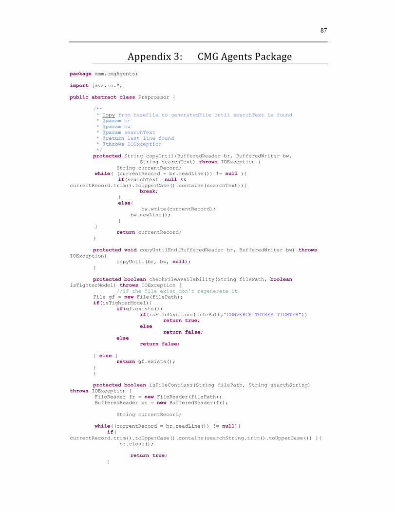
87
Appendix 3: CMG Agents Package
package mmm.cmgAgents;
import java.io.*;
public abstract class Preprossor {
/**
* Copy from baseFile to generatedFile until searchText is found
* @param br
* @param bw
* @param searchText
* @return last line found
* @throws IOException
*/
protected String copyUntil(BufferedReader br, BufferedWriter bw,
String searchText) throws IOException {
String currentRecord;
while( (currentRecord = br.readLine()) != null ){
if(searchText!=null &&
currentRecord.trim().toUpperCase().contains(searchText)){
break;
}
else{
bw.write(currentRecord);
bw.newLine();
}
}
return currentRecord;
}
protected void copyUntilEnd(BufferedReader br, BufferedWriter bw) throws
IOException{
copyUntil(br, bw, null);
}
protected boolean checkFileAvailability(String filePath, boolean
isTighterModel) throws IOException {
//if the file exist don't regenerate it
File gf = new File(filePath);
if(isTighterModel){
if(gf.exists())
if(isFileContians(filePath,"CONVERGE TOTRES TIGHTER"))
return true;
else
return false;
else
return false;
} else {
return gf.exists();
}
}
protected boolean isFileContians(String filePath, String searchString)
throws IOException {
FileReader fr = new FileReader(filePath);
BufferedReader br = new BufferedReader(fr);
String currentRecord;
while((currentRecord = br.readLine()) != null){
if(
currentRecord.trim().toUpperCase().contains(searchString.trim().toUpperCase()) ){
br.close();
return true;
}
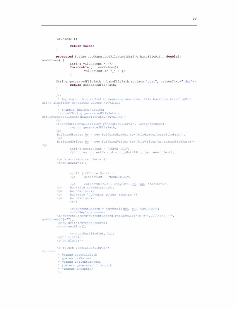
88
}
br.close();
return false;
}
protected String getGeneratedFileName(String baseFilePath, double[]
newValues) {
String valuesText = "";
for(double g : newValues){
valuesText += "_" + g;
}
String generatedFilePath = baseFilePath.replace(".dat", valuesText+".dat");
return generatedFilePath;
}
/**
* Implement this method to Generate new model file based on baseFilePath
using algorithm generated values newValues
*
* Example implementation:
*<code>String generatedFilePath =
getGeneratedFileName(baseFilePath,newValues);
<p>
if(checkFileAvailability(generatedFilePath, isTighterModel))
return generatedFilePath;
<p>
BufferedReader br = new BufferedReader(new FileReader(baseFilePath));
<p>
BufferedWriter bw = new BufferedWriter(new FileWriter(generatedFilePath));
<p>
String searchText = "PERMI ALL";
<p>String currentRecord = copyUntil(br, bw, searchText);
<p>bw.write(currentRecord);
<p>bw.newLine();
<p>if (isTighterModel) {
<p> searchText = "NUMERICAL";
<p> currentRecord = copyUntil(br, bw, searchText);
<p> bw.write(currentRecord);
<p> bw.newLine();
<p> bw.write("CONVERGE TOTRES TIGHTER");
<p> bw.newLine();
<p>}
<p>currentRecord = copyUntil(br, bw, "OPERATE");
<p>//Replace number
<p>currentRecord=currentRecord.replaceAll("[0-9\\,\\.\\+\\-]+",
newValues[0]+"");
<p>bw.write(currentRecord);
<p>bw.newLine();
<p>copyUntilEnd(br, bw);
<p>br.close();
<p>bw.close();
<p>return generatedFilePath;
</code>
* @param baseFilePath
* @param newValues
* @param isTighterModel
* @return generated file path
* @throws Exception
*/
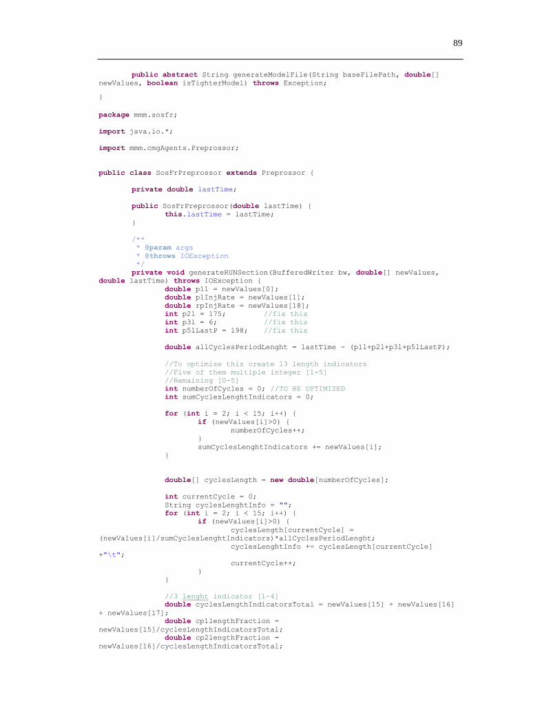
89
public abstract String generateModelFile(String baseFilePath, double[]
newValues, boolean isTighterModel) throws Exception;
}
package mmm.sosfr;
import java.io.*;
import mmm.cmgAgents.Preprossor;
public class SosFrPreprossor extends Preprossor {
private double lastTime;
public SosFrPreprossor(double lastTime) {
this.lastTime = lastTime;
}
/**
* @param args
* @throws IOException
*/
private void generateRUNSection(BufferedWriter bw, double[] newValues,
double lastTime) throws IOException {
double p1l = newValues[0];
double p1InjRate = newValues[1];
double rpInjRate = newValues[18];
int p2l = 175; //fix this
int p3l = 6; //fix this
int p5lLastP = 198; //fix this
double allCyclesPeriodLenght = lastTime - (p1l+p2l+p3l+p5lLastP);
//To optimize this create 13 length indicators
//Five of them multiple integer [1-5]
//Remaining [0-5]
int numberOfCycles = 0; //TO BE OPTIMIZED
int sumCyclesLenghtIndicators = 0;
for (int i = 2; i < 15; i++) {
if (newValues[i]>0) {
numberOfCycles++;
}
sumCyclesLenghtIndicators += newValues[i];
}
double[] cyclesLength = new double[numberOfCycles];
int currentCycle = 0;
String cyclesLenghtInfo = "";
for (int i = 2; i < 15; i++) {
if (newValues[i]>0) {
cyclesLength[currentCycle] =
(newValues[i]/sumCyclesLenghtIndicators)*allCyclesPeriodLenght;
cyclesLenghtInfo += cyclesLength[currentCycle]
+"\t";
currentCycle++;
}
}
//3 lenght indicator [1-4]
double cyclesLengthIndicatorsTotal = newValues[15] + newValues[16]
+ newValues[17];
double cp1lengthFraction =
newValues[15]/cyclesLengthIndicatorsTotal;
double cp2lengthFraction =
newValues[16]/cyclesLengthIndicatorsTotal;
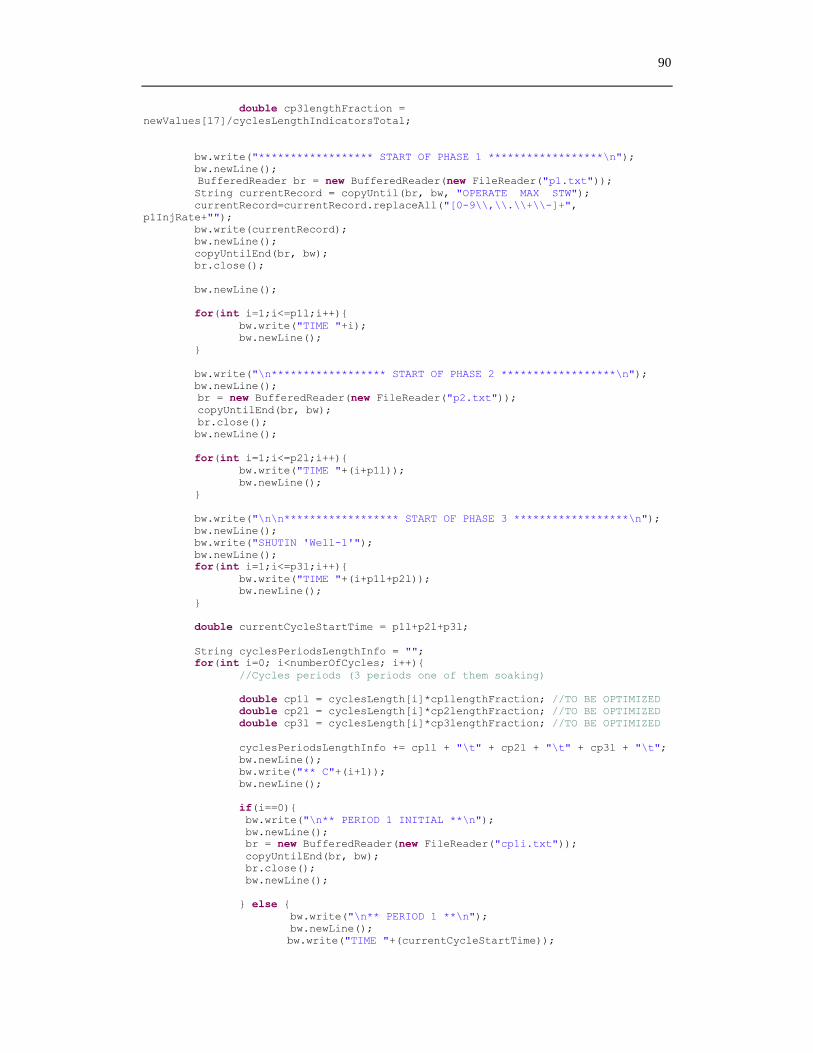
90
double cp3lengthFraction =
newValues[17]/cyclesLengthIndicatorsTotal;
bw.write("****************** START OF PHASE 1 ******************\n");
bw.newLine();
BufferedReader br = new BufferedReader(new FileReader("p1.txt"));
String currentRecord = copyUntil(br, bw, "OPERATE MAX STW");
currentRecord=currentRecord.replaceAll("[0-9\\,\\.\\+\\-]+",
p1InjRate+"");
bw.write(currentRecord);
bw.newLine();
copyUntilEnd(br, bw);
br.close();
bw.newLine();
for(int i=1;i<=p1l;i++){
bw.write("TIME "+i);
bw.newLine();
}
bw.write("\n****************** START OF PHASE 2 ******************\n");
bw.newLine();
br = new BufferedReader(new FileReader("p2.txt"));
copyUntilEnd(br, bw);
br.close();
bw.newLine();
for(int i=1;i<=p2l;i++){
bw.write("TIME "+(i+p1l));
bw.newLine();
}
bw.write("\n\n****************** START OF PHASE 3 ******************\n");
bw.newLine();
bw.write("SHUTIN 'Well-1'");
bw.newLine();
for(int i=1;i<=p3l;i++){
bw.write("TIME "+(i+p1l+p2l));
bw.newLine();
}
double currentCycleStartTime = p1l+p2l+p3l;
String cyclesPeriodsLengthInfo = "";
for(int i=0; i<numberOfCycles; i++){
//Cycles periods (3 periods one of them soaking)
double cp1l = cyclesLength[i]*cp1lengthFraction; //TO BE OPTIMIZED
double cp2l = cyclesLength[i]*cp2lengthFraction; //TO BE OPTIMIZED
double cp3l = cyclesLength[i]*cp3lengthFraction; //TO BE OPTIMIZED
cyclesPeriodsLengthInfo += cp1l + "\t" + cp2l + "\t" + cp3l + "\t";
bw.newLine();
bw.write("** C"+(i+1));
bw.newLine();
if(i==0){
bw.write("\n** PERIOD 1 INITIAL **\n");
bw.newLine();
br = new BufferedReader(new FileReader("cp1i.txt"));
copyUntilEnd(br, bw);
br.close();
bw.newLine();
} else {
bw.write("\n** PERIOD 1 **\n");
bw.newLine();
bw.write("TIME "+(currentCycleStartTime));
91
bw.newLine();
bw.write("shutin 'Well-3'");
bw.newLine();
bw.write("open 'Well-1'");
bw.newLine();
}
bw.write("\n** PERIOD 2 **\n");
bw.newLine();
bw.write("TIME "+(currentCycleStartTime+cp1l));
bw.newLine();
bw.write("shutin 'Well-1'");
bw.newLine();
bw.write("\n** PERIOD 3 **\n");
bw.newLine();
bw.write("TIME "+(currentCycleStartTime+cp1l+cp2l));
bw.newLine();
bw.write("open 'Well-3'");
bw.newLine();
currentCycleStartTime += cp1l+cp2l+cp3l;
}
bw.write("\n****************** START P5 ******************\n\n");
//String p5LastP = readFile("p5_lastP.txt"); //read p1
bw.newLine();
bw.write("TIME "+(currentCycleStartTime));
bw.newLine();
br = new BufferedReader(new FileReader("p5_lastP.txt"));
currentRecord = copyUntil(br, bw, "OPERATE MAX STW");
currentRecord=currentRecord.replaceAll("[0-9\\,\\.\\+\\-]+",
rpInjRate+"");
bw.write(currentRecord);
bw.newLine();
copyUntilEnd(br, bw);
br.close();
bw.newLine();
for(int i=1;i<=p5lLastP;i++){
bw.write("TIME "+(i+currentCycleStartTime));
bw.newLine();
}
br = new BufferedReader(new FileReader("lastPart.txt"));
copyUntilEnd(br, bw);
br.close();
bw.newLine();
bw.close();
System.out.println("FileInfo\t"+p1l+"\t"+p1InjRate+"\t"+rpInjRate+"\t"+allC
yclesPeriodLenght+"\t"+numberOfCycles
+"\t"+cp1lengthFraction+"\t"+cp2lengthFraction+"\t"+cp3lengthFraction+"\t"+
cyclesLenghtInfo+"CyclesPeriodsLength\t"+cyclesPeriodsLengthInfo);
}
@Override
public String generateModelFile(String baseFilePath, double[] newValues,
boolean isTighterModel) throws Exception {
String generatedFilePath =
getGeneratedFileName(baseFilePath,newValues);
if(checkFileAvailability(generatedFilePath, isTighterModel))
return generatedFilePath;
92
BufferedReader br = new BufferedReader(new FileReader(baseFilePath));
BufferedWriter bw = new BufferedWriter(new FileWriter(generatedFilePath));
String currentRecord = "";
if (isTighterModel) {
String searchText = "NUMERICAL";
currentRecord = copyUntil(br, bw, searchText);
bw.write(currentRecord);
bw.newLine();
bw.write("CONVERGE TOTRES TIGHTER");
bw.newLine();
}
currentRecord = copyUntil(br, bw, "RUN");
this.generateRUNSection(bw, newValues, lastTime);
br.close();
bw.close();
return generatedFilePath;
}
}
package mmm.cmgAgents;
public class GenericModelResult {
private double[] lastLineValues;
private double N;
private boolean isError;
/**
* @return the lastLineValues
*/
public double[] getLastLineValues() {
return lastLineValues;
}
/**
* @param lastLineValues the lastLineValues to set
*/
public void setLastLineValues(double[] lastLineValues) {
this.lastLineValues = lastLineValues;
}
/**
* @param lastLineValues the lastLineValues to set
*/
public void setLastLineValues(String[] lastLineValues) {
this.lastLineValues = new double[lastLineValues.length];
for (int i = 0; i < lastLineValues.length; i++) {
String string = lastLineValues[i];
this.lastLineValues[i] = Double.parseDouble(string);
}
}
/**
* @return the lastTime
*/
public double getLastTime() {
return lastLineValues[0];
}
93
/**
* @return the n
*/
public double getN() {
return N;
}
/**
* @param n the n to set
*/
public void setN(double n) {
N = n;
}
/**
* @return the isError
*/
public boolean isError() {
return isError;
}
/**
* @param isError the isError to set
*/
public void setError(boolean isError) {
this.isError = isError;
}
/* (non-Javadoc)
* @see java.lang.Object#toString()
*/
@Override
public String toString() {
String s = "";
for (double d : lastLineValues) {
s += d + "\t";
}
return s + N;
}
}
package mmm.cmgAgents;
import java.io.*;
public class SimulatorExecuter {
private String simulatorPath;
private String workDirectoryPath;
private String resultReportPath;
private String baseModelPath;
private int numberOfCores;
private boolean useParallelSolver;
private Preprossor preprossor;
private Postprossor postprossor;
private double lastTime;
public SimulatorExecuter(String simulatorPath, String workDirectoryPath,
String resultReportPath,
String baseModelPath, double lastTime, Preprossor
preprossor, Postprossor postprossor) {
this.simulatorPath = simulatorPath;
this.workDirectoryPath = workDirectoryPath;
this.resultReportPath = resultReportPath;
this.baseModelPath = baseModelPath;
this.numberOfCores = 1;
this.useParallelSolver = false;
this.preprossor = preprossor;
this.postprossor = postprossor;
94
this.lastTime = lastTime;
}
public SimulatorExecuter(String simulatorPath, String workDirectoryPath,
String resultReportPath,
String baseModelPath, double lastTime, int numberOfCores,
Preprossor preprossor, Postprossor postprossor) {
this(simulatorPath, workDirectoryPath, resultReportPath,
baseModelPath, lastTime, preprossor, postprossor);
this.numberOfCores = numberOfCores;
this.useParallelSolver = true;
}
private void execute(String filePath, int numberOfCores) {
// IF the output file exist it means model executed before!
// and not repeated in less number of cores because of ERROR
// No need to repeat execution
String irfFilePath = filePath.replace(".dat", ".irf");
File irfFile = new File(irfFilePath);
if (irfFile.exists() && numberOfCores == this.numberOfCores) {
return;
}
try {
String line;
String command = null;
if (useParallelSolver) {
command = "\"" + simulatorPath + "\" -f \"" +
filePath
+ "\" -wd \"" + workDirectoryPath +
"\" "
+ "-log -doms -parasol " +
numberOfCores + " -wait";
} else {
command = "\"" + simulatorPath + "\" -f \"" +
filePath
+ "\" -wd \"" + workDirectoryPath +
"\" " + "-log"
+ " -wait";
}
// System.out.println(command);
Process p = Runtime.getRuntime().exec(command);
// p.waitFor();
BufferedReader input = new BufferedReader(new
InputStreamReader(
p.getInputStream()));
while ((line = input.readLine()) != null) {
// System.out.println(line);
}
input.close();
} catch (Exception err) {
err.printStackTrace();
}
}
private String executeGenericResultReport(String irfFilePath, int
numberOfCores) throws Exception {
// create command file .rwd
String generatedFilePath = irfFilePath.replace(".irf", ".rwd");
String baseFileRWDFilePath = baseModelPath.replace(".dat", ".rwd");
String outputFilePath = irfFilePath.replace(".irf", ".rwo");
// if output is executed before don't repeat it
File of = new File(outputFilePath);
if (of.exists() && numberOfCores == this.numberOfCores)
return outputFilePath;
FileReader fr = new FileReader(baseFileRWDFilePath);
95
BufferedReader br = new BufferedReader(fr);
String currentRecord;
FileWriter fw = new FileWriter(generatedFilePath);
BufferedWriter bw = new BufferedWriter(fw);
while ((currentRecord = br.readLine()) != null) {
if (currentRecord.contains("*FILES")) {
currentRecord = "*FILES '" + irfFilePath + "' ";
}
bw.write(currentRecord);
bw.newLine();
}
br.close();
bw.close();
// run command file section
// generate output file
try {
String command = resultReportPath + " -f \"" +
generatedFilePath
+ " \" -o \"" + outputFilePath + "\"";
Process p = Runtime.getRuntime().exec(command);
BufferedReader input = new BufferedReader(new
InputStreamReader(
p.getInputStream()));
String line = "";
while ((line = input.readLine()) != null) {
// System.out.println(line);
}
input.close();
} catch (Exception err) {
err.printStackTrace();
}
return outputFilePath;
}
public GenericModelResult getGenericModelResults(double[] values)
throws Exception {
GenericModelResult r = getGenericModelResults(values,
this.numberOfCores, false);
return r;
}
private GenericModelResult getGenericModelResults(double[] values, int
numberOfCores, boolean isTighterModel)
throws Exception {
GenericModelResult r = new GenericModelResult();
// create model file
String generatedModelFilePath = null;
try{
generatedModelFilePath =
preprossor.generateModelFile(baseModelPath, values, isTighterModel);
} catch (IncorrectModelFileException ex){
String genesValuesText = "";
for(double g : values){
genesValuesText += g+ "\t";
}
generatedModelFilePath =
preprossor.getGeneratedFileName(baseModelPath, values);
96
File f = new File(generatedModelFilePath);
f.delete();
System.out.println("EXCEPTION\t"+ex.getMessage()+"; Unable
to generate a model for\t"+genesValuesText);
r.setError(true);
return r;
}
// execute generated model file
execute(generatedModelFilePath, numberOfCores);
// get result -- result report
String irfFilePath = generatedModelFilePath.replace(".dat",
".irf");
String generatedOutputFilePath = executeGenericResultReport(
irfFilePath, numberOfCores);
String[] lastLineValues = postprossor.getLastLine(
generatedOutputFilePath, "\t");
r.setLastLineValues(lastLineValues);
String outFilePath = generatedModelFilePath.replace(".dat",
".out");
r.setN(postprossor.getInitialOilInPlace(outFilePath));
if (r.getLastTime() != lastTime) {
if (isTighterModel && numberOfCores == 1){
r.setError(true);
} else if(numberOfCores == 1) {
r = getGenericModelResults(values, numberOfCores,
true);
if (r.getLastTime() != lastTime){
r.setError(true);
}
} else {
r = getGenericModelResults(values, numberOfCores/2,
isTighterModel);
}
}
return r;
}
/*
* (non-Javadoc)
*
* @see java.lang.Object#toString()
*/
@Override
public String toString() {
return "SimulatorExecuter \nsimulatorPath=\t" + simulatorPath
+ "\nworkDirectoryPath=\t" + workDirectoryPath
+ "\nresultReportPath=\t" + resultReportPath
+ "\nbaseModelPath=\t" + baseModelPath +
"\tPreprossor=\t"
+ preprossor;
}
}
package mmm.cmgAgents;
import java.io.*;
import java.util.regex.Matcher;
import java.util.regex.Pattern;
public class Postprossor {
97
public String[] getLastLine(String filePath, String delimiter) throws
Exception {
FileReader fr = new FileReader(filePath);
BufferedReader br = new BufferedReader(fr);
String currentRecord;
String lastRecord = "";
while((currentRecord = br.readLine()) != null)
lastRecord = currentRecord;
br.close();
return lastRecord.split(delimiter);
}
public double getInitialOilInPlace(String filePath) throws Exception {
FileReader fr = new FileReader(filePath);
BufferedReader br = new BufferedReader(fr);
String currentRecord;
boolean initialComponentInPlaceSectionFound=false;
double initialOilInPlace = -1;
while((currentRecord = br.readLine()) != null){
if(currentRecord.contains("TOTAL INITIAL COMPONENTS IN PLACE"))
initialComponentInPlaceSectionFound = true;
if(initialComponentInPlaceSectionFound &&
currentRecord.toUpperCase().contains("OIL")){
String scPattern = "([0-9\\,\\.\\+\\-]+)([Ee][0-9\\,\\.\\+\\-]+)";
Pattern p = Pattern.compile(scPattern);
Matcher m = p.matcher(currentRecord);
if (m.find()) {
initialOilInPlace = Double.parseDouble(m.group());
br.close();
return initialOilInPlace;
}
}
}
br.close();
return initialOilInPlace;
}
}
98
Appendix 4: Response surface proxy package
package mmm.responseSurfaceProxy;
import java.util.Hashtable;
public abstract class ResponseSurfaceProxy {
protected Hashtable<double[], Double> userValuesList;
public ResponseSurfaceProxy() {
userValuesList = new Hashtable<double[], Double>();
}
public abstract double getLinearResponse(double u[]);
public abstract double getNonLinearResponse(double[] useru);
public abstract void calculateLinearModel();
public abstract void calculateNonLinearModel();
public abstract void loadDynamicData();
public void addTrial(double[] uValues, double jValue){
if(!userValuesList.containsKey(uValues))
userValuesList.put(uValues, jValue);
}
}
package mmm.responseSurfaceProxy;
import java.io.*;
import java.util.Hashtable;
import Jama.*;
public class ResponseSurfaceProxyJama extends ResponseSurfaceProxy {
private Matrix Ulinear;
private Matrix UNonlinear;
private Matrix J;
private Matrix BetaLinear;
private Matrix BetaNonLinear;
public ResponseSurfaceProxyJama(String UfilePath, String JfilePath) throws
FileNotFoundException, IOException{
Matrix userMatrixU = Matrix.read(new BufferedReader(new
FileReader(UfilePath)));
Ulinear = getUFromUserMatrix(userMatrixU);
J = Matrix.read(new BufferedReader(new FileReader(JfilePath)));
}
public ResponseSurfaceProxyJama() {
userValuesList = new Hashtable<double[], Double>();
}
public double getLinearResponse(double u[]){
Matrix U = new Matrix(1, u.length+1);
for (int i = 0; i < u.length+1; i++) {
if(i==0)
U.set(0,i , 1);
else
U.set(0,i , u[i-1]);
}
Matrix r = getLinearResponse(U);
return r.get(0, 0);
}
/**
* @param U
* @return
99
*/
private Matrix getLinearResponse(Matrix U) {
Matrix r = U.times(BetaLinear);
return r;
}
public double getNonLinearResponse(double[] useru) {
double[] du = new double[useru.length+1];
double[] unl = getNonLinearDs(useru);
Matrix u = new Matrix(unl, 1);
Matrix r = getNonLinearResponse(u);
return r.get(0, 0);
}
private Matrix getNonLinearResponse(Matrix U) {
Matrix r = U.times(BetaNonLinear);
return r;
}
private Matrix getUFromUserMatrix(Matrix userMatrixU) {
double[][] uma = userMatrixU.getArray();
Matrix u = new Matrix(uma.length, uma[0].length+1);
for (int i = 0; i < uma.length; i++) {
for (int j = 0; j < uma[i].length+1; j++) {
if (j==0) {
u.set(i, j, 1);
} else {
u.set(i, j, uma[i][j-1]);
}
}
}
return u;
}
public void calculateLinearModel(){
if(Ulinear==null && J==null){
loadDynamicData();
}
BetaLinear = calculateBeta(Ulinear, J);
System.out.println("JandU\t\tActual J\tProxy J\tUs");
//print Y' values of initial data
Matrix r = getLinearResponse(Ulinear);
double[] rd = r.getColumnPackedCopy();
double[] actualJ = J.getColumnPackedCopy();
double summation = 0;
for (int i = 0; i < Ulinear.getRowDimension(); i++) {
System.out.print("JandU\t\t"+actualJ[i]);
System.out.print("\t"+rd[i]);
double dY1 = actualJ[i] - rd[i];
summation += Math.pow(dY1,2);
for (int j = 0; j < Ulinear.getColumnDimension();
j++) {
System.out.print("\t"+Ulinear.get(i, j));
}
System.out.println();
}
System.out.println("Linear Proxy L2[E]=" +
Math.pow(summation, 0.5) );
}
public void calculateNonLinearModel(){
if(Ulinear==null && J==null){
loadDynamicData();
}
calculateNonLinearU();
BetaNonLinear = calculateBeta(UNonlinear, J);
100
double[] b = BetaNonLinear.getColumnPackedCopy();
for (double d : b) {
System.out.println("Beta\t\t"+d);
}
System.out.println("JandU\t\tActual J\tProxy J\tUs");
//print Y' values of initial data
Matrix r = getNonLinearResponse(UNonlinear);
double[] rd = r.getColumnPackedCopy();
double[] actualJ = J.getColumnPackedCopy();
double summation = 0;
for (int i = 0; i < UNonlinear.getRowDimension(); i++) {
System.out.print("JandU\t\t"+actualJ[i]);
System.out.print("\t"+rd[i]);
double dY1 = actualJ[i] - rd[i];
summation += Math.pow(dY1,2);
for (int j = 0; j < UNonlinear.getColumnDimension(); j++) {
System.out.print("\t"+UNonlinear.get(i, j));
}
System.out.println();
}
System.out.println("Nonlinear Proxy L2[E]=" + Math.pow(summation,
0.5) );
}
/**
*
*/
public void loadDynamicData() {
//this means dynamic way is used
Matrix userMatrixU = null;
int currentCase = 0;
for (double[] u : userValuesList.keySet()) {
double response = userValuesList.get(u);
if(userMatrixU == null){
userMatrixU = new
Matrix(userValuesList.size(),u.length);
J = new Matrix(userValuesList.size(), 1);
}
for (int j = 0; j < u.length; j++) {
userMatrixU.set(currentCase, j, u[j]);
}
J.set(currentCase, 0, response);
currentCase++;
}
Ulinear = getUFromUserMatrix(userMatrixU);
}
/**
* @param U is the x or u values vector
* @param J is the y or j or the response vector
* @return
*/
private Matrix calculateBeta(Matrix U, Matrix J) {
if(U.getColumnDimension()<J.getRowDimension()){
//Over-determined
//Null space of U = 0
//U'U non-singular positive-definite matrix: (U'U)^-1 exists
// M < N -- U data less than J data
//B = (U' U)^-1 . U' . J
Matrix AA = U.transpose().times(U).inverse();
Matrix BB = U.transpose().times(J);
Matrix Beta = AA.times(BB);
return Beta;
} else {
//Under-determined
101
//rank of U = N
//Null space of U > 0
//UU' non-singular positive-definite matrix: (GG')^-1 exists
// M > N
//B = U' . (U . U')^-1 . J
Matrix AA = U.times(U.transpose()).inverse();
Matrix BB = U.transpose().times(AA);
Matrix Beta = BB.times(J);
return Beta;
}
}
private void calculateNonLinearU() {
Matrix subUL = Ulinear.getMatrix(0, Ulinear.getRowDimension()-1, 1,
Ulinear.getColumnDimension()-1);
double[][] u = subUL.getArray();
double[][] nonLinearU = new double[u.length][];
for (int i = 0; i < u.length; i++) {
nonLinearU[i] = getNonLinearDs(u[i]);
}
UNonlinear = new Matrix(nonLinearU);
}
private double[] getNonLinearDs(double[] ds) {
int countOfUUs=0;
for (int i = 1; i < ds.length+1; i++) {
for (int jj = 1; jj < ds.length+1; jj++) {
if(i<jj){
countOfUUs++;
//System.out.print("\tU"+i+ "U"+jj);
}
}
}
double[] nonLinearDs = new double[ds.length*2+countOfUUs+1];
int indexOfUUs=0;
nonLinearDs[0]=1;
for (int i = 1; i < ds.length+1; i++) {
nonLinearDs[i]=ds[i-1];
nonLinearDs[i+ds.length]=ds[i-1]*ds[i-1];
for (int jj = 1; jj < ds.length+1; jj++) {
if(i<jj){
indexOfUUs++;
nonLinearDs[ds.length*2+indexOfUUs]=ds[i-
1]*ds[jj-1];
}
}
}
return nonLinearDs;
}
}
102
Appendix 5: NOA reading package
public static double[][] getNOAArray(String filePath) throws IOException {
Jama.Matrix m = Matrix.read(new BufferedReader(new
FileReader(filePath)));
return m.getArray();
}
public static Population getInitialNAOPopulation(Configuration config,
String filePath) throws InvalidConfigurationException, IOException {
Population p = new Population(config);
double[][] d = getNOAArray(filePath);
for(int i=0; i<d.length; i++){
Gene[] garr = new Gene[d[i].length];
// Heating Phase length: multiple integer [60-790] days with
30 days
// level length
garr[0] = new MutipleIntegerGene(config, 60, 790, 30);
// Heating Phase steam injection rate
garr[1] = new DoubleGene(config, 10, 40);
// Cycles lengths indicators
garr[2] = new IntegerGene(config, 1, 5);
garr[3] = new IntegerGene(config, 1, 5);
garr[4] = new IntegerGene(config, 1, 5);
garr[5] = new IntegerGene(config, 1, 5);
garr[6] = new IntegerGene(config, 0, 5);
garr[7] = new IntegerGene(config, 0, 5);
garr[8] = new IntegerGene(config, 0, 5);
garr[9] = new IntegerGene(config, 0, 5);
garr[10] = new IntegerGene(config, 0, 5);
garr[11] = new IntegerGene(config, 0, 5);
garr[12] = new IntegerGene(config, 0, 5);
garr[13] = new IntegerGene(config, 0, 5);
garr[14] = new IntegerGene(config, 0, 5);
//garr[15] = new IntegerGene(config, 0, 5);
// Cycles periods (3 periods one of them soaking)
garr[15] = new IntegerGene(config, 1, 3);
garr[16] = new IntegerGene(config, 1, 3);
garr[17] = new IntegerGene(config, 1, 3);
// Recovery Phase steam injection rate
garr[18] = new DoubleGene(config, 10, 40);
for (int j = 0; j < d[i].length; j++) {
//garr[j] = new
MutipleIntegerGene(config,a_lowerBound,a_upperBound,a_significance);
if(j==1 || j==18){
double v = d[i][j];
garr[j].setAllele(v);
} else {
int v = (int)d[i][j];
garr[j].setAllele(v);
}
}
IChromosome c = new MyGenericChromosome(config,garr.length);
c.setGenes(garr);
p.addChromosome(c);
}
return p;
}