Embed Size (px)
Citation preview

University of Alberta
Acceleration of Transient Stability Simulation for Large-Scale Power Systems on Parallel and Distributed Hardware
by
Vahid Jalili-Marandi
A thesis submitted to the Faculty of Graduate Studies and Research in partial fulfillment of the requirements for the degree of
Doctor of Philosophy in
Energy Systems
Electrical and Computer Engineering
©Vahid Jalili-Marandi Fall 2010
Edmonton, Alberta
Permission is hereby granted to the University of Alberta Libraries to reproduce single copies of this thesis and to lend or sell such copies for private, scholarly or scientific research purposes only. Where the thesis is
converted to, or otherwise made available in digital form, the University of Alberta will advise potential users of the thesis of these terms.
The author reserves all other publication and other rights in association with the copyright in the thesis and,
except as herein before provided, neither the thesis nor any substantial portion thereof may be printed or otherwise reproduced in any material form whatsoever without the author's prior written permission.

Examining Committee Dr Venkata Dinavahi, Electrical and Computer Engineering Dr John Salmon, Electrical and Computer Engineering Dr Behrouz Nowrouzian, Electrical and Computer Engineering Dr Walid Moussa, Mechanical Engineering Dr William Rosehart, Electrical and Computer Engineering, University of Calgary

To my Grandpa
Haaj Jalil Jalili-Marandi and
my Parents for their Everlasting Supports

Abstract
Transient stability analysis is necessary for the planning, operation, and control of power
systems. However, its mathematical modeling and time-domain solution is computation-
ally onerous and has attracted the attention of power systems experts and simulation spe-
cialists for decades. The ultimate promised goal has been always to perform this simula-
tion as fast as real-time for realistic-sized systems.
In this thesis, methods to speedup transient stability simulation for large-scale power
systems are investigated. The research reported in this thesis can be divided into two parts.
First, real-time simulation on a general-purpose simulator composed of CPU-based com-
putational nodes is considered. A novel approach called Instantaneous Relaxation (IR) is
proposed for the real-time transient stability simulation on such a simulator. The moti-
vation of proposing this technique comes from the inherent parallelism that exists in the
transient stability problem that allows to have a coarse grain decomposition of resulting
system equations. Comparison of the real-time results with the off-line results shows both
the accuracy and efficiency of the proposed method. It is demonstrated that a power sys-
tem with 80 synchronous generators and 312 buses can be successfully modeled in detail
and run in real-time for the transient stability study by using 8 nodes of the PC-cluster
based simulator.
In the second part of this thesis, Graphics Processing Units (GPUs) are used for the first
time for the transient stability simulation of power systems. Data-parallel programming
techniques are used on the single-instruction multiple-date (SIMD) architecture of the GPU
to implement the transient stability simulations. Several test cases of varying sizes are
used to investigate the GPU-based simulation. The largest system that was implemented
on a single GPU consists of 1280 buses and 320 generators all modeled in detail. The
simulation results reveal the obvious advantage of using GPUs instead of CPUs for large-
scale problems.
In the continuation of part two of this thesis the application of multiple GPUs running
in parallel is investigated. Two different parallel processing based techniques are imple-

mented: the IR method, and the incomplete LU factorization based approach. Practical
information is provided on how to use multi-threaded programming to manage multiple
GPUs running simultaneously for the implementation of the transient stability simula-
tion. The implementation of the IR method on multiple GPUs is the intersection of data-
parallelism and program-level parallelism, which makes possible the simulation of very
large-scale systems with 7020 buses and 1800 synchronous generators.

Acknowledgements
I would like to express my sincere thanks to my supervisor Dr. Venkata Dinavahi for his
full support, patience, and guidance giving me throughout my research at the University
of Alberta. This thesis would not have been possible without encouragements and enthu-
siasms he created in me. He taught me the discipline of true research.
It is an honor for me to extend my gratitude to my PhD committee members Dr. Don
Koval, Dr. John Salmon, Dr. Behrouz Nowrouzian, Dr. Walied Moussa, and Dr. William Rose-
hart who read my thesis and gave me invaluable comments to improve and modify it.
Special thanks go to my colleagues and friends at the RTX-Lab: Babak Asghari, Md Omar
Faruque, Yuan Chen, Aung Myaing, and Lok-Fu Pak.
The PhD degree is not just about the research, and I would like to acknowledge all my
friends that I had their companionship during these years. I was lucky to have Aaron Ev-
eringham, Alireza Karimipour, Kathleen Forbes, Parisa Jalili-Marandi, Pouya Maraghechi, Reza
Moussavi Nik, Sahar Kolahi, Setareh Derakhshan, Vahid Farzamirad, Vahid Noei, and many oth-
ers with whom I had tones of exciting moments and joyful memories in Edmonton.
The last but not the least, I owe my deepest gratitude to my dearest ones who never
stopped supporting me: my parents, my siblings, Nazli and Sahand, my brother-in-law,
Khosrow, and my niece, Shanli. They are the happiness of my life.

Contents
1 Introduction 1
1.1 General Terms and Definitions . . . . . . . . . . . . . . . . . . . . . . . . . . 2
1.1.1 Transient . . . . . . . . . . . . . . . . . . . . . . . . . . . . . . . . . . . 2
1.1.2 Stability . . . . . . . . . . . . . . . . . . . . . . . . . . . . . . . . . . . 3
1.1.3 Transient Stability . . . . . . . . . . . . . . . . . . . . . . . . . . . . . 3
1.1.4 Real-Time Simulation . . . . . . . . . . . . . . . . . . . . . . . . . . . 5
1.2 Literature Review . . . . . . . . . . . . . . . . . . . . . . . . . . . . . . . . . . 6
1.3 Motivation for This Work . . . . . . . . . . . . . . . . . . . . . . . . . . . . . 9
1.4 Thesis Objectives . . . . . . . . . . . . . . . . . . . . . . . . . . . . . . . . . . 11
1.5 Thesis Outline . . . . . . . . . . . . . . . . . . . . . . . . . . . . . . . . . . . . 11
I Real-Time Transient Stability Simulation on CPU-based Hardware 13
2 Parallel Transient Stability Simulation Methods 14
2.1 Introduction . . . . . . . . . . . . . . . . . . . . . . . . . . . . . . . . . . . . . 14
2.2 Standard Method for Transient Stability Modeling . . . . . . . . . . . . . . . 15
2.3 Parallel Processor Architecture . . . . . . . . . . . . . . . . . . . . . . . . . . 20
2.3.1 PC-Cluster Based Real-Time Simulator . . . . . . . . . . . . . . . . . 22
2.3.2 Graphics Processing Unit . . . . . . . . . . . . . . . . . . . . . . . . . 23
2.4 Parallel Solution of Large-Scale DAEs Systems . . . . . . . . . . . . . . . . . 24
2.4.1 Tearing . . . . . . . . . . . . . . . . . . . . . . . . . . . . . . . . . . . . 26
2.4.2 Relaxation . . . . . . . . . . . . . . . . . . . . . . . . . . . . . . . . . . 26
2.5 Power System Specific Approaches . . . . . . . . . . . . . . . . . . . . . . . . 27
2.5.1 Diakoptics . . . . . . . . . . . . . . . . . . . . . . . . . . . . . . . . . . 28
2.5.2 Parallel-in-Space Methods . . . . . . . . . . . . . . . . . . . . . . . . . 28
2.5.3 Parallel-in-Time Methods . . . . . . . . . . . . . . . . . . . . . . . . . 31
2.5.4 Waveform Relaxation . . . . . . . . . . . . . . . . . . . . . . . . . . . 32

2.6 Power System Partitioning . . . . . . . . . . . . . . . . . . . . . . . . . . . . . 37
2.7 Types of Parallelism Used in This Thesis . . . . . . . . . . . . . . . . . . . . . 39
2.8 Summary . . . . . . . . . . . . . . . . . . . . . . . . . . . . . . . . . . . . . . . 40
3 The Instantaneous Relaxation (IR) Method 42
3.1 Introduction . . . . . . . . . . . . . . . . . . . . . . . . . . . . . . . . . . . . . 42
3.2 Limitations of WR method for Real-Time Transient Stability Simulation . . . 43
3.3 Instantaneous Relaxation . . . . . . . . . . . . . . . . . . . . . . . . . . . . . . 45
3.4 Coherency Based System Partitioning for the IR Method . . . . . . . . . . . 49
3.5 Implementation of IR Method . . . . . . . . . . . . . . . . . . . . . . . . . . . 50
3.5.1 Building of C-based S-Function . . . . . . . . . . . . . . . . . . . . . . 51
3.5.2 Off-Line Implementation of the IR Method . . . . . . . . . . . . . . . 53
3.5.3 Real-time Implementation of the IR Method . . . . . . . . . . . . . . 54
3.6 Experimental Results . . . . . . . . . . . . . . . . . . . . . . . . . . . . . . . . 57
3.6.1 Case Study 1 . . . . . . . . . . . . . . . . . . . . . . . . . . . . . . . . . 58
3.6.2 Case Study 2 . . . . . . . . . . . . . . . . . . . . . . . . . . . . . . . . . 61
3.6.3 Case Study 3: Large-Scale System . . . . . . . . . . . . . . . . . . . . 64
3.7 Summary . . . . . . . . . . . . . . . . . . . . . . . . . . . . . . . . . . . . . . . 65
II Large-Scale Transient Stability Simulation on GPU-based Hardware 68
4 Single GPU Implementation: Data-Parallel Techniques 69
4.1 Introduction . . . . . . . . . . . . . . . . . . . . . . . . . . . . . . . . . . . . . 69
4.2 GPU Overview . . . . . . . . . . . . . . . . . . . . . . . . . . . . . . . . . . . 70
4.2.1 GPU Evolution . . . . . . . . . . . . . . . . . . . . . . . . . . . . . . . 70
4.2.2 GPU Hardware Architecture . . . . . . . . . . . . . . . . . . . . . . . 71
4.2.3 GPU Programming . . . . . . . . . . . . . . . . . . . . . . . . . . . . . 73
4.3 Data-Parallel Computing . . . . . . . . . . . . . . . . . . . . . . . . . . . . . . 75
4.4 SIMD-Based Standard Transient Stability Simulation on the GPU . . . . . . 79
4.4.1 Standard Transient Stability Simulation . . . . . . . . . . . . . . . . . 79
4.4.2 SIMD Formulation for Transient Stability Solution . . . . . . . . . . . 80
4.5 GPU-Based Programming Models . . . . . . . . . . . . . . . . . . . . . . . . 82
4.5.1 Hybrid GPU-CPU Simulation . . . . . . . . . . . . . . . . . . . . . . . 82
4.5.2 GPU-Only Simulation . . . . . . . . . . . . . . . . . . . . . . . . . . . 83

4.6 Experimental Results . . . . . . . . . . . . . . . . . . . . . . . . . . . . . . . . 85
4.6.1 Simulation Accuracy Evaluation . . . . . . . . . . . . . . . . . . . . . 86
4.6.2 Computational Efficiency Evaluation . . . . . . . . . . . . . . . . . . 86
4.7 Discussion . . . . . . . . . . . . . . . . . . . . . . . . . . . . . . . . . . . . . . 88
4.8 Summary . . . . . . . . . . . . . . . . . . . . . . . . . . . . . . . . . . . . . . . 91
5 Multi-GPU Implementation of Large-Scale Transient Stability Simulation 92
5.1 Introduction . . . . . . . . . . . . . . . . . . . . . . . . . . . . . . . . . . . . . 92
5.2 Multi-GPU Overview . . . . . . . . . . . . . . . . . . . . . . . . . . . . . . . . 93
5.2.1 Applications . . . . . . . . . . . . . . . . . . . . . . . . . . . . . . . . . 93
5.2.2 Computing System Architecture . . . . . . . . . . . . . . . . . . . . . 93
5.2.3 Multi-GPU programming . . . . . . . . . . . . . . . . . . . . . . . . . 95
5.3 Implementation of Parallel Transient Stability Methods on Tesla S1070 . . . 98
5.3.1 Tearing Methods on Multi GPU . . . . . . . . . . . . . . . . . . . . . . 99
5.3.2 Relaxation Methods on Multiple GPUs . . . . . . . . . . . . . . . . . 101
5.4 Experimental Results . . . . . . . . . . . . . . . . . . . . . . . . . . . . . . . . 104
5.4.1 Work-station and Test Systems . . . . . . . . . . . . . . . . . . . . . . 104
5.4.2 Transparency . . . . . . . . . . . . . . . . . . . . . . . . . . . . . . . . 105
5.4.3 Scalability . . . . . . . . . . . . . . . . . . . . . . . . . . . . . . . . . . 107
5.4.4 LU Factorization Timing . . . . . . . . . . . . . . . . . . . . . . . . . . 108
5.5 Summary . . . . . . . . . . . . . . . . . . . . . . . . . . . . . . . . . . . . . . . 109
6 Summary and Conclusions 111
6.1 Contributions of This Thesis . . . . . . . . . . . . . . . . . . . . . . . . . . . . 112
6.2 Directions for Future Work . . . . . . . . . . . . . . . . . . . . . . . . . . . . . 112
Bibliography 115
Appendix A area1.c S-function Complete Source Code 123
Appendix B Performance Log for Real-time Simulation of a Large-Scale System 132
Appendix C Source Code for the GPU-only Modeling 138
Appendix D Tesla S1070 Manufacturer Data Sheet 153

Appendix E Single Line Diagram of Test Systems 160
E.1 Scale 1 . . . . . . . . . . . . . . . . . . . . . . . . . . . . . . . . . . . . . . . . 160
E.1.1 Load Data . . . . . . . . . . . . . . . . . . . . . . . . . . . . . . . . . 161
E.1.2 Generator Data . . . . . . . . . . . . . . . . . . . . . . . . . . . . . 162
E.1.3 Branch Data . . . . . . . . . . . . . . . . . . . . . . . . . . . . . . . 163
E.1.4 Transformer Data . . . . . . . . . . . . . . . . . . . . . . . . . . . 163
E.1.5 Load-Flow Results . . . . . . . . . . . . . . . . . . . . . . . . . . . 164
E.2 Scale 2 . . . . . . . . . . . . . . . . . . . . . . . . . . . . . . . . . . . . . . . . 165
E.3 Scale 4 . . . . . . . . . . . . . . . . . . . . . . . . . . . . . . . . . . . . . . . . 166
E.4 Scale 8 . . . . . . . . . . . . . . . . . . . . . . . . . . . . . . . . . . . . . . . . 167
E.5 Scale 16 . . . . . . . . . . . . . . . . . . . . . . . . . . . . . . . . . . . . . . . . 168
E.6 Scale 32 . . . . . . . . . . . . . . . . . . . . . . . . . . . . . . . . . . . . . . . . 169
E.7 Scale 64 . . . . . . . . . . . . . . . . . . . . . . . . . . . . . . . . . . . . . . . . 170
E.8 Scale 128 . . . . . . . . . . . . . . . . . . . . . . . . . . . . . . . . . . . . . . . 171
E.9 Scale 180 . . . . . . . . . . . . . . . . . . . . . . . . . . . . . . . . . . . . . . . 172

List of Tables
3.1 Performance log for real-time simulation of Case Study 1 . . . . . . . . . . . 61
3.2 Performance log for real-time simulation of Case Study 2 . . . . . . . . . . . 63
3.3 Relation between time-step and accuracy of the IR method . . . . . . . . . . 64
4.1 GeForce GTX 280 GPU specifications . . . . . . . . . . . . . . . . . . . . . . . 73
4.2 Systems data and simulations time . . . . . . . . . . . . . . . . . . . . . . . . 88
4.3 Speed-up comparison . . . . . . . . . . . . . . . . . . . . . . . . . . . . . . . . 90
5.1 Tesla T10 Processor specifications . . . . . . . . . . . . . . . . . . . . . . . . . 94
5.2 Single GPU timing . . . . . . . . . . . . . . . . . . . . . . . . . . . . . . . . . 100
5.3 Tesla T10 processor bandwidth test results . . . . . . . . . . . . . . . . . . . . 103
5.4 Test System Scales . . . . . . . . . . . . . . . . . . . . . . . . . . . . . . . . . . 105
5.5 Multi-GPU timing . . . . . . . . . . . . . . . . . . . . . . . . . . . . . . . . . . 109

List of Figures
1.1 (a) Real-Time and (b) Non-Real-Time or Off-Line simulation. . . . . . . . . . 6
2.1 Excitation system with AVR and PSS [47]. . . . . . . . . . . . . . . . . . . . . 17
2.2 Hardware architecture of the RTX-LAB real-time simulator . . . . . . . . . . 23
2.3 Connection of the GPU to a PC motherboard using the PCIe bus. . . . . . . 25
2.4 Applying Gauss-Jacobi relaxation at different level of equations . . . . . . . 27
2.5 The Gauss-Jacobi WR algorithm . . . . . . . . . . . . . . . . . . . . . . . . . . 34
2.6 The RLC circuit. . . . . . . . . . . . . . . . . . . . . . . . . . . . . . . . . . . . 35
2.7 Response of the RLC circuit . . . . . . . . . . . . . . . . . . . . . . . . . . . . 36
2.8 Application of windowing technique in the WR method . . . . . . . . . . . 37
2.9 Flowchart of the WR method . . . . . . . . . . . . . . . . . . . . . . . . . . . 38
2.10 Integrating various types of parallelism . . . . . . . . . . . . . . . . . . . . . 40
3.1 Partitioning a large system into subsystems. . . . . . . . . . . . . . . . . . . . 44
3.2 Real-time implementation of the WR method: Option 1. . . . . . . . . . . . . 46
3.3 Real-time implementation of the WR method: Option 2. . . . . . . . . . . . . 46
3.4 Flowchart of the proposed IR method . . . . . . . . . . . . . . . . . . . . . . 49
3.5 SIMULINK S-function flowchart . . . . . . . . . . . . . . . . . . . . . . . . . 52
3.6 Top lay-out of a decomposed system for off-line simulation . . . . . . . . . . 54
3.7 Placing S-function in subsystem Area1 for off-line simulation. . . . . . . . 55
3.8 Monitoring and saving outputs of the decomposed system. . . . . . . . . . . 56
3.9 Configuration of the real-time simulator . . . . . . . . . . . . . . . . . . . . . 57
3.10 Lay-out of a three-area decomposed system for real-time simulation . . . . 58
3.11 Placing S-function in subsystem Area1 for real-time implementation. . . . 59
3.12 One-line diagram for Case Study 1. . . . . . . . . . . . . . . . . . . . . . . . . 59
3.13 Distribution Case Study 1 in real-time simulator nodes . . . . . . . . . . . . 60
3.14 Comparison Case Study 1 results with PSS/E . . . . . . . . . . . . . . . . . . 61

3.15 One-line diagram for Case Study 2. . . . . . . . . . . . . . . . . . . . . . . . . 62
3.16 Distribution Case Study 2 in real-time simulator nodes . . . . . . . . . . . . 63
3.17 Comparison Case Study 2 results with PSS/E . . . . . . . . . . . . . . . . . . 64
3.18 Comparison Case Study 2 results with PSS/E . . . . . . . . . . . . . . . . . . 65
3.19 Large-scale Case Study . . . . . . . . . . . . . . . . . . . . . . . . . . . . . . . 67
4.1 Hardware architecture of GPU mounted on the PC motherboard. . . . . . . 72
4.2 The GTX 280 hardware architecture . . . . . . . . . . . . . . . . . . . . . . . 74
4.3 Cooperation of the host and device . . . . . . . . . . . . . . . . . . . . . . . . 76
4.4 An schematic model for a limiter. . . . . . . . . . . . . . . . . . . . . . . . . . 78
4.5 Flowchart for the hybrid GPU-CPU transient stability simulation . . . . . . 84
4.6 Flowchart for the GPU-only transient stability simulation . . . . . . . . . . . 85
4.7 Comparison of results with PSS/E: part 1 . . . . . . . . . . . . . . . . . . . . 87
4.8 Comparison of results with PSS/E: part 2 . . . . . . . . . . . . . . . . . . . . 87
4.9 Computation time variation with respect to system scale. . . . . . . . . . . . 89
4.10 Speed-up of GPU-based processing. . . . . . . . . . . . . . . . . . . . . . . . 90
5.1 Front and top views of Tesla S1070 . . . . . . . . . . . . . . . . . . . . . . . . 95
5.2 Inside architecture of Tesla S1070 . . . . . . . . . . . . . . . . . . . . . . . . . 96
5.3 Host Interface Card . . . . . . . . . . . . . . . . . . . . . . . . . . . . . . . . . 96
5.4 Possible configurations of connecting Tesla S1070 to host . . . . . . . . . . . 97
5.5 Serial and parallel kernel execution . . . . . . . . . . . . . . . . . . . . . . . . 98
5.6 Programming application for general purpose multi-GPU computation . . . 99
5.7 ILU method . . . . . . . . . . . . . . . . . . . . . . . . . . . . . . . . . . . . . 101
5.8 ILU-based tearing method implementation on multiple GPUs. . . . . . . . . 102
5.9 IR method implementation on multiple GPUs. . . . . . . . . . . . . . . . . . 104
5.10 Multi-GPU simulation: (a) 2 GPUs, (b) 4 GPUs. . . . . . . . . . . . . . . . . . 106
5.11 Scaling factor for the IR and ILU methods using 2 GPUs. . . . . . . . . . . . 108
5.12 Scaling factor for the IR and ILU methods using 4 GPUs. . . . . . . . . . . . 109
E.1 Scale 1 system: 39 buses, 10 generators. . . . . . . . . . . . . . . . . . . . . . 160
E.2 Scale 2 system: 78 buses, 20 generators. . . . . . . . . . . . . . . . . . . . . . 165
E.3 Scale 4 system: 156 buses, 40 generators. . . . . . . . . . . . . . . . . . . . . . 166
E.4 Scale 8 system: 312 buses, 80 generators. . . . . . . . . . . . . . . . . . . . . . 167
E.5 Scale 16 system: 624 buses, 160 generators. . . . . . . . . . . . . . . . . . . . 168

E.6 Scale 32 system: 1248 buses, 320 generators. . . . . . . . . . . . . . . . . . . . 169
E.7 Scale 64 system: 2596 buses, 640 generators. . . . . . . . . . . . . . . . . . . . 170
E.8 Scale 128 system: 4992 buses, 1280 generators. . . . . . . . . . . . . . . . . . 171
E.9 Scale 180 system: 7020 buses, 1800 generators. . . . . . . . . . . . . . . . . . 172

List of Acronyms
CPU Central Processing UnitCUDA Compute Unified Device ArchitectureGPU Graphics Processing UnitILU Incomplete LUIR Instantaneous RelaxationMIMD Multiple-Instruction-Multiple-DataRTW Real-Time WorkshopSFU Special Function UnitSIMD Single-Instruction-Multiple-DataSM Streaming MultiprocessorSP Stream ProcessorTPC Thread Processing ClusterWR Waveform RelaxationXHP eXtra High Performance

1Introduction
Electric power systems are large and complex. The complexity of power systems arises
from the interactions of several devices that are involved in the system such as generators,
transmission and distribution networks, and electrical loads. The generators are intercon-
nected via the transmission lines and cover vast geographical areas. Continuous growth
in electricity demand and consequent expansion of the power systems are creating newer
and larger problems. Therefore, power engineers are always exploring methods for quick
and efficient solutions for these problems.
Maintaining system stability is very important in order to have a secure and continuous
operation of the power system. Loss of supply following system instability would result in
massive economic losses to both the power producers as well as customers. Dynamic sta-
bility analysis preforms simulations of the impact of potential electric grid fault conditions
after a grid disturbance (contingency) in a transient time frame, which is normally up to
about 10 seconds after a disturbance. When a grid is subjected to a disturbance, active and
reactive powers of generators oscillate for a few seconds following the disturbance. These
oscillations must be damped out to regain a stable operating condition. Contingency con-
ditions studied include “normal” transmission line outages and/or power plant outages
caused by acts of nature or equipment (e.g., due to lightning), “wear and tear” (e.g., equip-
ment age failures) and outage conditions caused by human error or potential equipment
failures. Any specific contingency simulation analysis can take several minutes of com-
puter time, even when simulating only a few seconds of grid response after a “what if”
1

disturbance. Thus, analyzing hundreds or more of such “what if” contingencies can take
hours of calculations [1].
A major issue facing the electric utility industry today is to perform the aforementioned
calculations for a large-scale power system in a much shorter time interval so that the cal-
culations can be performed on-line as changes occur based on real-time data, rather than
performing the calculations off-line during days, weeks or even months ahead of time.
This large amount of computer time occurs because the transient phenomena have to be
calculated over a 5 to 10 seconds time interval for a large interconnected power system
based on detailed dynamic mathematical models of grid components. These analyses are
currently conducted off-line since the simulation must be run for each condition of a large
set of all contingency conditions that might occur. Using a software tool developed by
EPRI [2], the computer time to perform hundreds of contingency simulations was reduced
to about 20 to 30 minutes. However, improved numerical methods and computer systems
are still needed today, to reduce this computational time to less than 5 to 10 minutes. This
will meet the requirements for the promised real-time dynamic stability analysis, which
could then become a powerful tool for system operation. By using such a tool in the en-
ergy management centers the operators would quickly evaluate a large number of poten-
tial harmful contingencies and determine which ones could cause unacceptable system
instabilities. Thus, operators would have the opportunity to figure out appropriate con-
trol actions that could prevent the grid from having a regional or multi-regional cascading
blackout.
1.1 General Terms and Definitions
In this section1 the important terms used in this thesis are defined to clearly identify the
scope of work done in this research.
1.1.1 Transient
The IEEE Standard Dictionary defines a transient phenomena as [3]:
Pertaining to or designating a phenomenon or a quantity that varies between two consecutive
steady states during a time interval that is short compared to the time scale of interest. A transient
can be a unidirectional impulse of either polarity or a damped oscillatory wave with the first peak
1Material from this section has been published: V. Jalili-Marandi, V. Dinavahi, K. Strunz, J. A. Martinez,and A. Ramirez, “Interfacing techniques for transient stability and electromagnetic transient programs,” IEEETrans. on Power Delivery, vol. 24, no. 4, pp. 2385-2395, Oct. 2009.
2

occurring in either polarity.
Overvoltages due to lightning and capacitor energization are examples of events that
cause impulsive and oscillatory transients, respectively. Some of the most common types
of transient phenomena in power systems include energization of transmission lines, switch-
ing off of reactors and unloaded transformers, linear resonance at fundamental or at a
harmonic frequency, series capacitor switching and sub-synchronous resonance, and load
rejection [4].
1.1.2 Stability
From a system point of view there exist several types of stability definitions such as:
Lyapunov stability, input-output stability, stability of linear systems, and partial stabil-
ity [5]. Kimbark has classically defined stability related to power systems in [6], however,
this definition was restricted to synchronous machines, and their being “in step”. The
IEEE/CIGRE Joint Task Force on Stability Terms and Definitions [5] adopted the following
definition:
Power system stability is the ability of an electric power system, for a given initial operating
condition, to regain a state of operating equilibrium after being subjected to a physical disturbance,
with most system variables bounded so that practically the entire system remains intact.
Instability in power systems can be caused by either small or large disturbances. Dur-
ing a small disturbance the set of equations which describe the perturbed power system
can be linearized; however, during the large disturbance these equations cannot be lin-
earized for the purpose of analysis [7]. Typical examples of small disturbances are a small
change in the scheduled generation of one machine, or a small load (say 1/100 of system
capacity or less) disconnected or added to the network [8, 9]. Severe perturbations such as
short-circuit faults and loss of generation events are representative of large disturbances.
Additionally, phenomena which cause instability problems in power systems have been
sub-classified based on their duration. Two types of time frame are recognizable: short
term and long term. The period of interest to stability assessment of a network perturbed
by a short term instability event is in the order of few seconds (3 to 20 seconds); however,
this time span extends to several or many minutes for the long term one [5].
1.1.3 Transient Stability
Power system stability phenomena can be categorized into three major classes: rotor angle
stability, voltage stability, and frequency stability. If an interconnected network has been
3

subjected to a perturbation; the ability of this power system to keep its machines in syn-
chronism, and to maintain voltages of all buses as well as the frequency of the whole net-
work around the steady-state values is the basis for the above mentioned classification [10].
Each form of stability phenomena may be caused by a small or large disturbance.
Although in the literature the term transient stability has been used to refer to the large-
disturbance rotor angle stability phenomenon [7, 8], some authors have used this term as
a general purpose stability study of the given network with a particular disturbance se-
quence [11]. The IEEE/CIGRE task force report has categorized both the small and large
disturbance rotor angle stability phenomena as short-term events. Furthermore, it recom-
mends the term transient stability for large-disturbance rotor angle stability phenomenon,
with a time frame of interest in the order of 3 to 5s following the disturbance. This time
span may increase up to 10-20s in the case of very large networks with dominant inter-area
swings [5].
The complete power system model for transient stability analysis can be mathemat-
ically described by a set of first-order differential equations and a set of algebraic equa-
tions. The differential equations model dynamics of the rotating machines while the alge-
braic equations represent the transmission system, loads, and the connecting network [12].
Chapter 2 provides details of the basic approach and numerical methods required for the
solution of the transient stability problem.
A complete description of the power network dynamic behavior requires a very large
number of equations. For instance, consider a realistic inter-connected power system
which includes over 3000 buses and about 400 power stations which are feeding 800 loads.
Assuming that the transmission system and loads are modeled by algebraic equations, and
the generation stations are modeled by a set of 20 first-order differential equations each.
The transient stability analysis of the described network needs solving of 8000 differential
equations and about 3500 algebraic equations [9,13]. To make this solution as time-efficient
as possible usually a time-step in the range of a few milliseconds is chosen for the simula-
tion. In transient stability studies it is assumed that voltage and current waveforms more
or less remain at power frequency (60 or 50 Hz). Thus, for modeling the electrical parts of
the power system steady-state voltage and current phasors can be used. Moreover, tran-
sient stability study is a positive-sequence single-phase type of analysis [4, 14].
4

1.1.4 Real-Time Simulation
The term “real-time” has been traditionally used by the computer industry to refer to in-
teractive systems where the computer response is sufficiently fast enough to satisfy human
users. A more rigorous definition is applied to digital control schemes where the computer
response must occur at specific time intervals. In the case of power system simulation, this
implies that the computer must solve the model equations within the model time step [15].
In general, real-time digital simulation may be defined as a faithful reproduction of output
waveforms, by combining systems of hardware and software, that would be identical to
the waveforms or effects produced by the real power system being modeled. Depending
on the time taken by the computer to complete the computation of state outputs for each
time-step two situations can arise. As shown in Figure 1.1(a), if the execution time, Te, for
the simulation of any time-step is smaller or equal to the time-step used, the simulation is
said to be real-time simulation. On the other hand, as shown in Figure 1.1(b), if Te for any
time-step is greater than its time-step, the simulation is said to be non-real-time or off-line
and in that case, execution time overruns take place. If such a situation is observed, the
simulation time-step should be increased or the system model should be modified to fit
the execution time within the time-step.
Analog scaled-down simulator also known as Transient Network Analyzers (TNAs),
were the predecessors of fully digital real-time simulators. However, realization of large-
scale power systems with a high level of complexity, non-linearity, and sophisticated dy-
namic elements using TNAs is practically impossible [16]. Real-time digital simulation is a
state-of-the-art technique for simulation of power systems and their components. During
the last ten to fifteen years, significant efforts have been made to develop real-time digital
simulators of power system networks. Developments of high speed computers and other
devices accelerated the research in this area. The approach in digital simulation provides
accuracy in component modeling and flexibility in component interconnection for repre-
sentation of a power system. The system is modeled with the help of a software using
graphical interface on a workstation or a personal computer (PC) and then simulated on a
powerful parallel processor based PC cluster.
Real-time simulation can be classified into two categories [17]: (1) Fully digital real-
time simulation and (2) Hardware-In-the-Loop (HIL) real-time simulation. A fully digital
real-time simulation requires the entire system (including control, protection and other ac-
cessories) to be modeled inside the simulator and the simulation to be completed within
5

tn tn+1 tn+2
real-time
clock
fixed time-step
simulator
time
overrun
fixed time-step
idle
time
execution
time: Te
simulator
time(a)
(b)
Figure 1.1: (a) Real-Time and (b) Non-Real-Time or Off-Line simulation.
the specified time-step. In this type of simulation, no I/Os or external interfacing is nec-
essary (except those required for monitoring the simulation results). On the other hand,
Hardware-In-the-Loop (HIL) simulation refers to a simulation, where parts of the fully dig-
ital real-time simulation have been replaced with actual physical components. In this case,
the simulation proceeds with the device-under-test connected through input and output
interfaces such as filters, Digital-to-Analog (D/A) and Analog-to-Digital (A/D) convert-
ers, signal conditioners etc. The simulation can also be modified with the user defined
control inputs, for example closing or opening of switches to connect or disconnect the
components in the simulated power system.
Fully digital simulation is often used for the understanding of behavior of a system un-
der certain circumstances resulting from external or internal dynamic influences, however,
HIL simulation is used to minimize the risk of investment through the use of a prototype
once the underlying theory is established with the help of fully digital real-time simula-
tion. Fully digital simulation is the type of real-time simulation that is used in this thesis.
1.2 Literature Review
Transient instability has long been recognized as the dominant problem in power system
operation. It has been extensively studied since the 1920s and a lot of knowledge and expe-
rience is available in the literature [5]. Transient stability study is important for planning,
design, operation, control, and post-disturbances analysis in power systems [10].
6

From the system theory viewpoint, power systems transient stability is a strongly non-
linear problem. To assess it accurately, first it should be mathematically described by a set
of differential-algebraic equations (DAEs) as follows:
x = f(x,V, t) (1.1)
0 = g(x,V, t) (1.2)
x(t0) = x0 (1.3)
where x is the vector of state variables, x0 is the initial values of state variables, and
V is the vector of bus voltages. Equation (1.1) describes the dynamic behavior of the sys-
tem, while equation (1.2) describes the network constraints on (1.1). Solution of these
equations in time-domain requires employing numerical integration methods. Histori-
cally, time-domain methods have been used even before the advent of numerical comput-
ers where calculations of simplified or reduced versions of the system dynamic equations
were carried out manually to extract the machines’ rotor angle evolution with time, known
as swing curves [18]. Another approach of evaluating transient stability is a graphical
method, popularized in 1930s, as known as “equal-area criterion”. This method deals with
a one-machine system connected to an infinite bus or any two-machine system, whether it
actually has only two machines or more than two machines reduced to two-machine equiv-
alent. The method studied stability by using the concept of energy. The equal-area method
is still used to provide insight into the physical concept of the transient stability phenom-
ena, and for evaluating the various system parameters [19, 20]. Further information about
other types of approaches that have been developed based on the energy concept is avail-
able in [21].
Exploring the transient stability literature reveals that the efforts on the acceleration of
the simulation have been twofold. One is on the algorithms and numerical method, and
the other is on the hardware architecture. From the algorithm viewpoint there has been
extensive research done on solving equations (1.1) and (1.2) with accuracy and efficiency.
The overall solution can be classified into two groups [12]: partitioned and simultaneous
solution approaches. In the partitioned solution the differential equation set (1.1) is solved
separately for the state variables and the equation set (1.2) is solved for the algebraic vari-
ables, and these solutions are then alternated. In the simultaneous approaches, however,
an implicit integration method converts the (1.1) into a set of algebraic equations, and then
this set is lumped into the (1.2) resulting in a larger set of algebraic equations including all
7

the variables. In each of these approaches one can use various type of integration meth-
ods. The explicit Runge-Kutta [22], predictor-corrector method [23], implicit multi-step
integration [24] are some example methods that have been exploited for the partitioned
approaches. For the simultaneous approaches the multi-step integration methods and the
trapezoidal rule have been used widely [25, 26].
The complexity of power systems simulation has increased with the system size. It
was found that a single computer cannot handle the simulation of ever expanding power
systems since it is time critical. Therefore, the need for parallel processing in the transient
stability simulation of realistic systems was recognized to reduce computational complex-
ity. The diakoptics method introduced by Kron [27] tears the problem into several subtasks
that can be run concurrently on parallel computers. In parallel-in-space [28] and waveform
relaxation [29] methods the system is decomposed into smaller subsystems and the com-
putation is allocated to parallel computers. There are also parallel-in-time methods [30,31]
which concurrently solve multiple time steps on parallel processors. While parallel pro-
cessing usually refers to simulation techniques in which closely coupled processors are
simultaneously working on the transient stability computation, the concept of distributed
processing employs a number of loosely coupled and geographically distributed computers
to simulate large-scale power systems [32].
From the hardware point of view several types of MIMD (Multiple-Instruction Multiple-
Data) and SIMD (Single-Instruction Multiple-Data) parallel architectures [33] have been
employed to accelerate transient stability simulation. Supercomputers [34], multiprocessor
networks [35, 36], array-processors [37, 38], and PC-cluster based real-time simulators [39]
all have been examined and reported for this application. Although these hardware-based
approaches helped to speed-up the simulations, they were stymied by significant draw-
backs. The cost of the supercomputers, communication issues and difficulties in the control
of multiprocessor-based systems, difficulties in the programming and required algorithms
for fitting in array-processors, and limitation on maximum system size of the simulated
networks in real-time simulators are some of the noteworthy bottlenecks which limited
their widespread application.
The new capability of the modern GPU, as a massively parallel processor, for gen-
eral purpose high performance computation is the beginning of a new era in computing
science. Although at first glance the SIMD architecture of the GPUs and that of array-
processors might look similar, there are significant differences between these two technolo-
gies. Moreover, issues related to processing elements’ communication overhead, program-
8

ming complexity, and cost effectiveness have been solved for the GPU [40]. The advantages
of modern GPUs, the demand for fast simulation, and the structure of the transient stabil-
ity computation makes the GPU very suitable for this application.
1.3 Motivation for This Work
In power system operations, the operators strive to operate the systems with a high degree
of reliability. Reliability refers to the ability of the system to supply adequate electricity
service on a nearly continuous basis, with few interruptions over an extended time pe-
riod [5]. The key to have a reliable system operation is to maintain satisfactory security at
all times. Unlike reliability that is measured as performance over a period of time, security
refers to the degree of risk in a power system’s ability to survive contingencies without
interruption to customer service at any instant of time. The security of a power system
can be assessed by simulating potential disturbances and determining if the disturbances
will cause any adverse impacts that could result in unsafe condition in the network. How-
ever, in many cases a “static security assessment” or “static contingency analysis” can not
achieve the necessary security under changing grid and generation conditions. For this
purpose the “dynamic security assessment” (DSA) tools are employed, which take a snap-
shot of the system condition, perform comprehensive security assessment, and provide
operators with warning of abnormal situations as well as remedial recommendations. The
main objective of DSA tools is to determine if the system can tolerate a set of major contin-
gencies, which falls under purview of transient stability analysis [41].
The need of real-time assessment of dynamic stability analysis was highlighted by the
recent black out in USA (August 14, 2003) and Italy (September 28, 2003). The August 14
black-out in USA and Canada affected 50 million people. It took a day to restore power to
New York City, and almost two days to restore power to Detroit. The Italian black-out, the
worst blackout in Europe that affected 57 million people, started with 6545 MW import to
Italy. In less than 3 minutes cascading phenomena isolated the Italian system from Europe,
loss of generation in Italy and insufficient load shedding resulted in system black-out. The
phenomena occurred in less than 3 minutes, but it has been proceeded by about 15 min-
utes within which the problem evolved from a normal situation to an alert and then to an
emergency state with a restoration time of 19 hours. A list of evolving factors was collected
from which it was identified that improved power system monitoring and preventive ac-
tions are the most important items [42]. Presently, in most utilities, the dynamic security
9

analyses are conducted by off-line studies. However, there is an increasing demand for fast
and real-time simulations which can be incorporated within the energy management sys-
tem to determine the critical system limits based on the current conditions of the system.
This is a particular application where speed of simulation is vital.
The need to accelerate transient stability simulations for realistic size power systems is
the main driving force for this research. The speed of transient stability simulations can be
improved by three approaches:
• Developing new algorithmic methods
• Exploiting parallel and distributed processors
• Utilizing faster processors
While the transient stability simulation tools have been improved over the last two
decades, the improvement has been mainly made in the modeling complexity and user
friendliness rather than in the structure of the algorithm. It was predicted in 1993 that
the impact of new mathematical methods or algorithms in power system analysis will be
at best evolutionary and not revolutionary [43]. It was a true prediction at least for the
transient stability simulation. Although adaptations such as dishonest Newton-Raphson,
innovations such as sparsity handling and optimal ordering, and efficient coding brought
computer analysis of large-scale power systems into practical use, the basic time domain
algorithm for transient stability simulation remained the most reliable method for the com-
mercial and industry software developers [44]. Therefore, after many years of experience
in the transient stability simulation methods, as described in the literature review, no one
expects that a novel approach on a single processor could significantly alleviate the simula-
tion time, unless it somehow exploits a specific hardware architecture. Against the gradual
improvements of the algorithmic methods, the hardware improvements have been revo-
lutionary. These improvements includes processor architecture design, such as evolving
multi-core CPUs and GPUs, the processor’s speed, and advancements in the peripheral
technology such as storage devices and communication equipment.
This thesis aggregates all three aforementioned approaches to accelerate of transient
stability simulation of large-scale power systems. A novel algorithmic method is pro-
posed and implemented on two different types of processors. One is a general purpose
CPU-processor based state-of-the-art real-time digital simulator, and the other is the mas-
sively parallel Graphics Processing Unit (GPU). The CPU-based processor has a sequential
architecture, while GPU has a data-parallel design.
10

1.4 Thesis Objectives
The previous sections gave a glimpse of the transient stability problem and the wide efforts
made in this area. It can be concluded that in the transient stability analysis fast and reli-
able simulation is never enough and more is always required by the industry. The objective
of this thesis is to investigate the use of parallel processing based approaches to accelerate
transient stability simulation of large-scale systems. To achieve this purpose first we will
focus on the real-time simulation on a PC-cluster real-time simulator by introducing and
implementing a novel method. This can lead us to configure a real-time simulator that is
specifically designed for transient stability analysis, such as existing ones for the electro-
magnetic studies, but one that is much more cost effective. In the second part of this thesis
the use of single and multiple GPUs for the large-scale transient stability simulations is
investigated. It is predicted that GPUs will be at the core of the near future massive com-
putational engines. Therefore, power system software developers should be aware of the
GPU applications in the power system computations and exploit it.
1.5 Thesis Outline
The thesis consists of six chapters. Each chapter discuses a particular topic of relevance to
the thesis and the contributions made are described.
• Chapter 1: Introduction - The general terms used in this thesis are described in this
chapter to highlight the scope of the research. The background work done in this area
since several decades ago is summarized by considering both software and hardware
developing aspects. The applications of transient stability analysis in the planning
and operation of power systems are discussed which justified the need for faster tran-
sient stability simulations. The desire to accelerate the transient stability simulation
for large-scale power systems is the main motivation of this thesis.
• Chapter 2: Parallel Transient Stability Simulation Methods - The purpose of this
chapter is to provide a basis for the thesis. It begins with the transient stability
problem formulation and the standard solution method to model this phenomena
in power systems. However, the focus in this chapter is to review the application of
parallel processing based technology used up to date of preparing this dissertation.
This application includes both the algorithmic aspects as well as hardware advance-
ments.
11

• Chapter 3: The Instantaneous Relaxation (IR) Method - The Instantaneous Relax-
ation (IR) method is introduced and implemented in this chapter. The objective is to
revisit the application of real-time digital simulators to the transient stability prob-
lem. By exploiting the parallelism inherent in the transient stability problem, a paral-
lel solution algorithm can be devised to maximize the computational efficiency of the
real-time simulator. This would reduce the cost of the required hardware for a given
system size or increase the size of the simulated system for a fixed cost and hardware
configuration. To demonstrate the performance of the IR method, three case studies
have been implemented on a PC-Cluster based real-time simulator and the results
are validated by the PSS/E software. Several comparisons verified the accuracy and
efficiency of the IR method.
• Chapter 4: Single GPU Implementation: Data-Parallel Techniques - In this chapter
we discuss GPU-based transient stability simulation for large-scale power systems.
The mathematical complexity along with the large data crunching need in the tran-
sient stability simulation, and the substantial opportunity to exploit parallelism are
the motivations to use GPU in this area. However, since the GPU’s architecture is
markedly different from that of a conventional CPU, it requires a completely differ-
ent algorithmic approach for implementation. This chapter investigates the poten-
tial of using a GPU to accelerate this simulation by exploiting its SIMD architecture.
Two SIMD-based programming models to implement the standard method of the
transient stability simulation were proposed and implemented on a single GPU. The
simulation codes are written entirely in C++ integrated with GPU-specific functions.
• Chapter 5: Multi-GPU Implementation of Large-Scale Transient Stability Simula-
tion - The main goal in this chapter is to demonstrate the practical aspects of utilizing
multiple GPUs for large-scale transient stability simulation. Two parallel processing
based techniques are implemented on a Tesla S1070 unit. The techniques used here
are from tearing and relaxation categories, explained in Chapters 2 and 3. The exper-
imental results revealed that program level decomposition, as it happens in the IR
method, is more efficient than task level decomposition.
• Chapter 6: Summary and Conclusions - The contribution of this research are sum-
marized in this chapter. Some plans for the future work are suggested here.
12

Part I
Real-Time Transient StabilitySimulation on CPU-based Hardware
13

2Parallel Transient Stability Simulation Methods
2.1 Introduction
In Chapter 1, the applications of transient stability analysis in the planning and operation
of power systems are discussed which justified the needs for faster transient stability sim-
ulations. As mentioned, for several decades it was known that the single-processor based
methods are not effective for the simulation of large-scale power systems. Thus, to achieve
substantial improvement in the speed of transient stability simulation parallel processing
approaches have been chosen as the most promising methods. In this chapter we will
discuss the issues related to the parallel simulation of the transient stability on two fronts
(1) parallel processor’s hardware architecture, and (2) parallel processing based transient
stability algorithms.
The chapter starts with the transient stability problem formulation and numerical meth-
ods for solution in the time-domain. Then, it will discuss the general classifications exist-
ing for hardware architecture of the parallel processors, and continue with introducing
state-of-the-art hardware utilized in this thesis. A review of the parallel-processing-based
algorithms for the solution of differential-algebraic equations, (DAEs) and their specific
application for the transient stability problem will be described in the remainder of this
chapter.
14

2.2 Standard Method for Transient Stability Modeling
The AC transmission network responds rapidly to any change in load or network topology.
The time constant associated with the network variables are extremely small and can be
assumed to be negligible in transient stability analysis without significant loss of accuracy
[45]. In transient stability the concern is electromechanical oscillation, that is the variation
in power output of machines as their rotors oscillate. The time constants associated with
the rotors are of the order 1 to 10 seconds. Therefore, the differential equations that are
relevant in this analysis are dominated by those having time constants of this order.
A widely used method for detailed modeling of the synchronous generator for the
transient stability simulation is the Park’s equations with an individual dq reference frame
fixed on the generator’s field winding [8]. The network side, including transmission lines
and loads, is modeled using algebraic equations in a common DQ reference frame. Rep-
resentation of AVR and PSS increases the number of differential equations and hence the
complexity of the model. However, the validity of the dynamic response in a network
with a lot of interconnections and in a time frame of a few seconds highly depends on
the accuracy of the generator model and other components which can have effects on the
dynamics of the system. Realistic interconnected power systems are generally supervised
and maintained regionally by the control centers located in different geographical places.
Therefore, fully detailed models for the transient stability studies are imperative for both
online and offline simulations [46]. In this work the detailed model of synchronous gen-
erator including AVR and PSS is used. Each generating unit is modeled using a 9th order
Park’s model with an individual dq reference frame fixed on the generator’s field wind-
ing [8]. The network, including transmission lines and loads, is modeled using algebraic
equations in a common DQ reference frame. The complete system representation used in
this thesis is summarized here:
1. Equations of motion (swing equations or rotor mechanical equations):
δ(t) = ωR.∆ω(t) (2.1)
∆ω(t) =1
2H[Te(t) + Tm −D.∆ω(t)].
2. Rotor electrical circuit equations: This model includes two windings on the d axis
(one excitation field and one damper) and two damper windings on the q axis.
ψfd(t) = ωR.[efd(t)−Rfdifd(t)] (2.2)
15

ψ1d(t) = −ωR.R1di1d(t)
ψ1q(t) = −ωR.R1qi1q(t)
ψ2q(t) = −ωR.R2qi2q(t).
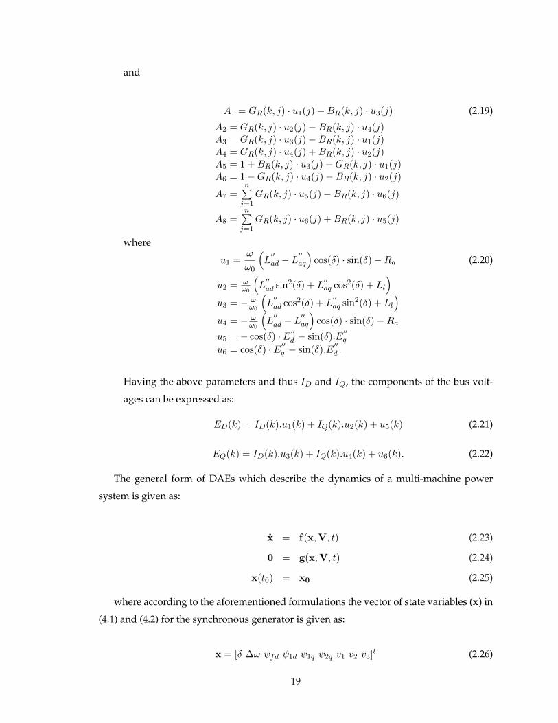
3. Excitation system: Figure 2.1 shows ST1A type excitation system [47]. This system
includes an AVR and PSS.
v1(t) =1
TR[vt(t)− v1(t)] (2.3)
v2(t) = Kstab.∆ω(t)− 1Tw
v2(t)
v3(t) =1T2
[T1v2(t) + v2(t)− v3(t)].
4. Stator voltage equations:
ed(t) = −Raid(t) + L′′q iq(t)− E′′d (t) (2.4)
eq(t) = −Raid(t)− L′′did(t)− E′′q (t)
where
E′′d ≡ Laq[
ψq1
Lq1+
ψq2
Lq2] (2.5)
E′′q ≡ Lad[
ψfd
Lfd+
ψd1
Ld1].
5. Electrical torque:
Te = −(ψadiq − ψaqid) (2.6)
where
ψad = L′′ad[−id +ψfd
Lfd+
ψd1
Ld1] (2.7)
16

STABK
W
W
sT
sT
1 2
1
1
1
sT
sT
RsT1
1AK
maxFE
minFE
fdE
refV
tE
maxsv
minsv
2v 3v
sv
1v +
+
-
Exciter
Terminal voltage
transducer
WashoutGain
Phase
compensation
Figure 2.1: Excitation system with AVR and PSS [47].
ψaq = L′′aq[−iq +ψq1
Lq1+
ψq2
Lq2].
where ωR, H , D, Rfd, R1d, R1q, R2q, Ra, Lfd, Ld1, Lq1, Lq2, L′′d, L′′q , Lad, Laq, L′′ad, L′′aq,
TR, Tw, T1, T2, and Kstab are constant system parameters whose definition can be
found in [9].
6. Network equations [8]: Stator equations are solved together with the network equa-
tions. All nodes except the generator nodes are eliminated and the admittance matrix
for the reduced network is obtained. The procedure for network reduction is shown
below. The nodal equation for the network can be written as:
I = Y V (2.8)
where I(n+r)×1 = [In×1... 0r×1]t. n denotes the number of generator nodes and r
denotes the number of remaining nodes. The matrices Y and V are partitioned as:
[In
0r
]=
[Ynn Ynr
Yrn Yrr
] [Vn
Vr
]. (2.9)
Expanding (2.9) to find In based on Vn we obtain:
In = (Ynn − YnrY−1rr Yrn)Vn (2.10)
Thus,
In = YR.En (2.11)
17

where the matrix YR = Ynn − YnrY−1rr Yrn is the desired reduced matrix. It has the
dimensions n×n where n is the number of generators. This matrix must be computed
for steady-state, during the transient state, and after the clearing of the transient
phenomena.
As the components in the network common DQ frame are of interest the above com-
plex matrix equation can be written as two separate real matrix equations:
IDn = GR.EDn −BR.EQn (2.12)
IQn = GR.EQn + BR.EDn. (2.13)
To relate the components of voltages and currents expressed in the d, q reference of
each individual machine to the common reference frame (DQ), the following refer-
ence frame transformation is used:
idq = IDQ · exp(−jδ) (2.14)
edq = EDQ · exp(−jδ) (2.15)
where δ is the rotor angle of the synchronous machine.
The kth iteration current components in the common reference frame can be ex-
pressed as [48]:
ID(k) =1
A5(S1 + S2 + A7) (2.16)
IQ(k) =1
A6(S3 + S4 + A8) (2.17)
where the S and A parameters are defined as below:
S1 =n∑
j=1j 6=k
ID(j).A1, S2 =n∑
j=1
IQ(j).A2 (2.18)
S3 =n∑
j=1
ID(j).A3, S4 =n∑
j=1j 6=k
IQ(j).A4
18
and
A1 = GR(k, j) · u1(j)−BR(k, j) · u3(j) (2.19)
A2 = GR(k, j) · u2(j)−BR(k, j) · u4(j)A3 = GR(k, j) · u3(j)−BR(k, j) · u1(j)A4 = GR(k, j) · u4(j) + BR(k, j) · u2(j)A5 = 1 + BR(k, j) · u3(j)−GR(k, j) · u1(j)A6 = 1−GR(k, j) · u4(j)−BR(k, j) · u2(j)
A7 =n∑
j=1GR(k, j) · u5(j)−BR(k, j) · u6(j)
A8 =n∑
j=1GR(k, j) · u6(j) + BR(k, j) · u5(j)
where
u1 =ω
ω0
(L′′ad − L
′′aq
)cos(δ) · sin(δ)−Ra (2.20)
u2 = ωω0
(L′′ad sin2(δ) + L
′′aq cos2(δ) + Ll
)
u3 = − ωω0
(L′′ad cos2(δ) + L
′′aq sin2(δ) + Ll
)
u4 = − ωω0
(L′′ad − L
′′aq
)cos(δ) · sin(δ)−Ra
u5 = − cos(δ) · E′′d − sin(δ).E
′′q
u6 = cos(δ) · E′′q − sin(δ).E
′′d .
Having the above parameters and thus ID and IQ, the components of the bus volt-
ages can be expressed as:
ED(k) = ID(k).u1(k) + IQ(k).u2(k) + u5(k) (2.21)
EQ(k) = ID(k).u3(k) + IQ(k).u4(k) + u6(k). (2.22)
The general form of DAEs which describe the dynamics of a multi-machine power
system is given as:
x = f(x,V, t) (2.23)
0 = g(x,V, t) (2.24)
x(t0) = x0 (2.25)
where according to the aforementioned formulations the vector of state variables (x) in
(4.1) and (4.2) for the synchronous generator is given as:
x = [δ ∆ω ψfd ψ1d ψ1q ψ2q v1 v2 v3]t (2.26)
19

and x0 is the initial values of state variables, and V is the vector of bus voltages.
(4.1) describes the dynamic behavior of the system, while (4.2) describes the network con-
straints on (4.1). The standard approach to solve these nonlinear and coupled DAEs in-
volves three steps [12]:
• Step 1. The continuous-time differential equations are first discretized and con-
verted to discrete-time algebraic equations. Using the implicit Trapezoidal integra-
tion method, discretizing (4.1) results in a new set of non-linear algebraic equations:
0 =h
2[f(x,V, t) + f(x,V, t− h)]− (x(t)− x(t− h)) (2.27)
where h is the integration time-step.
• Step 2. The existing non-linear algebraic equations are linearized by the Newton-
Raphson method (for the jth iteration) as:
J(zj−1) ·∆z = −F(zj−1) (2.28)
where J is the Jacobian matrix, z = [x,V], ∆z = zj − zj−1, and F is the vector of
nonlinear function evaluations.
• Step 3: The resulting linear algebraic equations are solved to obtain the system state.
(4.5) is solved using the LU factorization followed by the forward-backward substi-
tution method.
2.3 Parallel Processor Architecture
A sequential computer with one CPU (central processing unit) includes only one control
instruction unit. Apart from its limitation to single instruction execution at any time, there
were two main obstacles with this technology: slow memory access and fundamental lim-
itations such as overheating with compact circuits. These issues limited the achievable
speed of serial computers even with the growth of the hardware technology. Therefore,
the parallel processing techniques were seriously taken into account as the main alterna-
tive approach. As reported in the IEEE committee report [49]:
“Parallel processing is a form of information processing in which two or more processors to-
gether with some form of inter-processor communication system, co-operate on the solution of a
problem”.
20

In parallel processing the single CPU is replaced by multiple CPUs (even if they are
individually slower than the presumed single CPU) whose overall parallel performance
accelerates the simulation.
Chronologically, there are two famous taxonomies for classification of the parallel pro-
cessing architecture hardware. The first one was made by Flynn [33] in which computing
machines are characterized by the number of simultaneously active instruction and data
streams. The two practically used groups are Single-Instruction Multiple-Data (SIMD)
and Multiple-Instruction Multiple-Data (MIMD) architectures. In a SIMD-based technol-
ogy the parallelism is exploited by performing the same operation concurrently on many
pieces of data, while in the MIMD architecture different operations may be performed si-
multaneously on many pieces of data. The SIMD model works best on a certain set of
problems such as image processing, and MIMD is suitable for general purpose computa-
tion. Vector processors and array processors are examples of the SIMD-based architecture,
multi-processor and PC clusters have an MIMD architecture.
The other taxonomy was made by Gurd [50] in which rather than concentrating on the
number of active instruction streams, the focus is on the relationship between processing
elements and memory modules. Based on this taxonomy there are two classes of parallel
processing architectures: distributed memory, and shared memory. In the former, there is
no memory in the system other than the local memory on each processing element, and the
processors communicate with each other by sending and receiving messages in a network
with topologies such as mesh, ring, or hypercube. An example of these processors is Intel
iPSC/2 hypercube machine which also has been used in the transient stability simulation
of power systems. It consists of a host computer as the cube-manager, and 32 processors
(nodes). Each node is directly connected to only d−1 nodes, where d is the cube dimension.
The host processor loads the execution program into all nodes and sends all the necessary
data to each processor, where the solution is performed in parallel. The results are sent
back to the host. Successful simulation on these machines requires the decomposition of
the problem into loosely coupled tasks and distribute them among the processors. The
communication between nodes is by sending messages.
In the shared memory processors, however, there is a central memory accessible from
any of the processing units, regardless of existing local memory on each processing units.
The common memory is used to make communications between processors in shared
memory architecture. The Alliant FX/8 is an example of these machines that contains 8
Computational Elements and 64MB of shared memory.
21

This dissertation involves two state-of-the-art parallel hardware architecture: PC-Cluster
based real-time simulator, and Graphics Processing Unit (GPU). The former is a CPU-
based simulator whose details on architecture and configuration will be explained in this
section. The architecture of GPU, however, is substantially different from that of the CPU-
based processors. Thus, GPU will be introduced in this chapter, and it will be explained in
detail in Chapter 4.
2.3.1 PC-Cluster Based Real-Time Simulator
The real-time simulator existing in the RTX-LAB at the University of Alberta is manu-
factured by OPAL-RT Technologies Inc. using commercial-off-the-shelf components. It
mainly comprises of two groups of computers known as target nodes, and hosts. Target
nodes are the computational cores which carry out the simulation, and each of them is
powered by a dual 3.0GHz Intel XeonTM processor. Each host is a high-performance com-
puter which has a 3.0GHz Intel Pentium IV CPU to offer fast loading and compilation
of the developed models, and providing the interface between the user and the simulator.
The high-speed communication links connect targets, as well as hosts and targets. External
hardware can also be connected to the simulator via the FPGA-based (Field-Programmable
Gate Array) analog/digital inputs/outputs.
The hardware architecture of the real-time simulator is shown in Figure 2.2. The two
processors, i.e. CPUs, in one target communicate with each other through shared memory.
The targets is also capable of eXtreme High Performance (XHP) mode execution, in which
one CPU is dedicated entirely to the computation while the other CPU is running real-
time operating system tasks and schedulers. Several state-of-the-art computer networking
technologies have been utilized to achieve the best communication throughput:
• Shared memory for inter-processor communication in one target. It has the lowest
latency.
• InfiniBand architecture for inter-target communication. It has low latency (from sev-
eral to several-ten microsecond) depending on communication data size.
• SignalWire which only links adjacent two targets. It has only several-microsecond
level of latency.
• Giga-speed Ethernet which mainly connects between targets and hosts, or among
hosts.
22

Target Cluster
Hosts
External Hardware
External Hardware
Host 1
FPGA 1 (Signal Conditioning)
FPGA n (Signal Conditioning)
Shared
Memory
CPU 1
CPU 2
Cluster Node 2 (Dual XEON)
Shared
Memory
CPU 1
CPU 2
Cluster Node 1 (Dual XEON)
Shared
Memory
CPU 1
CPU 2
Cluster Node n (Dual XEON)
I N F I N I B A N D
L I N K
S I G N A L
W I R E
G I G A B I T
E T H E R N E T
Host 2
Host n
Figure 2.2: Hardware architecture of the RTX-LAB real-time simulator [51].
This high-performance PC-cluster based real-time simulator, which has a shared-memory
MIMD architecture, enables any general purpose parallel processing based simulation and
specifically the digital real-time simulation. Other companies such as RTDS Technologies
Inc. and Hypersim have also manufactured similar real-time using distributed sequential
processors. The philosophy of the real-time simulation, its necessity, and requirement will
appear in the next chapter.
2.3.2 Graphics Processing Unit
Recently, Graphics Processing Units (GPUs), which were originally developed for ren-
dering detailed real-time visual effects in the video gaming industry, have become pro-
grammable to the point where they are a viable general purpose programming platform.
General purpose programming on the GPU (also called GPGPU) is currently getting a lot
of attention in the various scientific communities due to the low cost and huge compu-
23

tational horsepower of the recent GPUs. The use of GPGPU techniques as an alternative
to the parallel CPU-based cluster of computers in simulations that need highly intensive
computations has become a real possibility.
Figure 2.3 illustrates schematic of how the GPU and CPU hardware are connected. As
shown in this figure, GPU is mounted to the PC motherboard similar to the other add-in
peripheral cards. The fundamental idea of the GPU is exploiting the parallel processing.
The GPU executes independently from the CPU but it is controlled by CPU. Application
program running on CPU uses the driver software to communicate with the GPU. The
many-core architecture of GPU, that will be discussed in detail in Chapter 4, is especially
suited for problems that can be expressed as fine-grained data-parallel computations. Ex-
cept the field of image rendering, which GPU was originally designed for, several other
fields from the signal processing and physics simulation to computational finance and bi-
ology have also exploited GPUs to accelerate their simulations.
The modern GPU consists of multiprocessors which map the data elements to the par-
allel processing threads. The multiprocessor creates, manages, and executes concurrent
threads in hardware with zero scheduling overhead. The fast barrier synchronization with
lightweight thread creation and zero-overhead thread scheduling supports fine-grained
parallelism. To manage hundreds of threads the multiprocessors map each thread to one
scaler processor core, and each scaler thread executes independently with its own instruc-
tion. There is a global device memory that all the multiprocessors can have access to. Also,
each multiprocessor has its own on-chip memory that is accessible individually. Overall,
the GPU can be categorized as an SIMD and shared memory processor. However, there are
significant differences between SIMD structure of the GPU and that of the array processors
which will be explained in Chapter 4.
2.4 Parallel Solution of Large-Scale DAEs Systems
A common approach for time-domain simulation of a physical system, described by a set
of non-linear DAE consists of three steps: an integration method (e.g. trapezoidal rule)
for discretizing the differential equations, an iterative method (e.g. Newton-Raphson) for
solving the non-linear algebraic equations, and a linear equation solver such as Gaussian
Elimination and Back Substitution. This traditional approach is referred to as the standard
or direct simulation approach [52]. Both the storage and CPU time required by the standard
approach grow rapidly with the size of the system, measured in terms of its components
24

System Memory
6-15GB/s
PC Motherboard
Processing
ElementsCache40GB/s
CPU Processing
Elements
GPU Memory
20-140GB/s
GPU
1-8GB/s
Figure 2.3: Connection of the GPU to a PC motherboard using the PCIe bus.
(i.e. generators in the case of a power system), increases. The demand for simulating
ever larger systems brought the use of parallel architectures to the forefront of researchers
minds. Clearly, exploitation of such parallel hardware was not possible unless appropriate
software was developed that fits the architecture. Moreover, in a large system of DAEs dif-
ferent variables change at different rates. In the standard approach the integration method
is forced to discretize all the differential equation with the same time-step which must be
small enough to capture the fastest dynamics in the system. As such simulating realistic-
size large-scale systems using the standard approach became very time consuming. To
address these problems, a family of techniques known as domain decomposition was devel-
oped.
Domain decomposition refers to any technique that divides a system of equations into
several subsets that can be solved individually using conventional numerical methods. To
solve a set of non-linear differential-algebraic equations domain decomposition can be ap-
plied at any of the three levels of equations, i.e. differential equations, non-linear algebraic
equations, and linear algebraic equations. In these techniques the system of equations at
each level is viewed as a composition of several subsystems at the same level that have
interaction together. The subsystem is a subset of system variables. When the system is
decomposed into subsystems, the solution of each subsystem is carried out by using the
conventional numerical techniques existed for each level of equations. The advantage of
decomposition techniques is that they are suitable for parallel hardware architectures since
several subsystems can be solved simultaneously.
To describe the structure of a system the notion of the dependency matrix (D) is used.
25

For a system with n equations and n unknown variables, D is an n × n matrix whose
elements are 1 or 0. If the ith equation involves the jth variable, then D(i, j) is 1, otherwise
D(i, j) = 0.
Two different approaches were proposed in the literature to perform domain decom-
position: tearing and relaxation.
2.4.1 Tearing
Tearing (introduced as the diakoptics method by G. Kron [27]) is the approach that takes
advantage of the block structure of the system of equations. For a system of equations
in which the dependency matrix is sparse, i.e. D has a small percentage of 1’s, tearing
can be used to achieve decomposition while maintaining the numerical properties of the
method used to solve the system. The Bordered Blocked Diagonal (BBD) form is one spe-
cific structure suitable for this approach. Tearing decomposition at the level of linear alge-
braic equations can be implemented as the Block LU Factorization method, and at the level
of non-linear algebraic equations as the Multilevel Newton-Raphson method [53].
It should be noted that the computational efficiency of this approach over the standard
approach depends critically on the structure of the system, and it does not increase when
system dependency matrix is dense. However, the numerical properties of the tearing ap-
proach are the same as those of the standard numerical methods applied to the system
without using decomposition. For example, in nonlinear algebraic equations the Multi-
level Newton-Raphson method still has the same local quadratic rate of convergence the
same as that of the conventional full Newton-Raphson method.
2.4.2 Relaxation
Relaxation [54] is an approach which is not restricted to a particular system structure. In
this approach the system is partitioned into a number of subsystems based on either the
system equations or component connectivity. Solving these subsystems is always easier
than solving the original system. Therefore, the complexity will be reduced regardless
of the system sparsity. Within each subsystem the variables to be solved for are called
internal variables and the other variables involving in that subsystem are referred as external
variables, which are internal variables of other subsystems. To solve a subsystem for its
internal variables the values of its external variables are first guessed and then updated
through an iterative procedure.
Two well known iterative schemes used for relaxation decomposition are the Gauss-
26

Gauss-Jacobi
Relaxation
0),,...,,,,...,,( 121211 =uxxxxxxfnn
&&&
0),,...,,,,...,,( 221212 =uxxxxxxfnn
&&&
0),,...,,,,...,,( 2121 =nnnnuxxxxxxf &&&
0),,...,,,,...,,( 1
11
21
11
211 =−−−−uxxxxxxf
k
n
kkk
n
kk&&&
0),,...,,,,...,,( 2
1
2
1
1
1
2
1
12 =−−−−uxxxxxxf
k
n
kkk
n
kk&&&
0),,...,,,,...,,( 1
2
1
1
1
2
1
1 =−−−−
n
k
n
kkk
n
kk
nuxxxxxxf &&&
Gauss-Jacobi
Relaxation
0),,...,,( 1211 =uxxxgn
0),,...,,( 2212 =uxxxgn
0),,...,,( 21 =nnnuxxxg
0),,...,,( 1
11
211 =−−uxxxg
k
n
kk
0),,...,,( 2
1
2
1
12 =−−uxxxg
k
n
kk
0),,...,,( 1
2
1
1 =−−
n
k
n
kk
nuxxxg
Gauss-Jacobi
Relaxation
0... 1121 211 1 =++++ uxxxnn
ααα
0... 2222 212 1 =++++ uxxxnn
ααα
0...2211 =++++nnn nnnuxxx ααα
0... 1
1
1
1
212111 =++++−−uxxx
k
nn
kkααα
0... 22222
1
121 =++++−
uxxxk
nn
kkααα
0...1
22
1
11 =++++−−
n
k
nnn
k
n
k
nuxxx ααα
(b)
(a)
(c)
Figure 2.4: Applying Gauss-Jacobi relaxation at different level of equations: (a) differentialequations, (b) non-linear algebraic equations, (c) linear algebraic equations.
Seidel and Gauss-Jacobi methods [55]. Relaxation can be used at each level of the solution.
Figure 2.4 gives an example of using Gauss-Jacobi relaxation at different levels of equa-
tions. The application of this approach for nonlinear algebraic equations can be found
in [28, 30]. Relaxation can be used at the level of differential equations as well, but it is not
straightforward. In this case, the system is broken into subsystems in a way that the com-
ponents inside of each subsystem (internal variables) are strongly interdependent while
the dependency between components in two different subsystems (internal and external
variables) is weak enough to ignore their interconnection. In other words, the subsystems
can be relaxed. Therefore, each part of the system is still a system of differential equations
but with a smaller size that can be solved in the time-domain using the standard approach.
The relaxation approach applied to the differential equations’ level has been known as the
Waveform Relaxation (WR) method, which is discussed later in this chapter.
2.5 Power System Specific Approaches
The previous section provided a review of the parallel-processing-based computational
approaches for a general case of DAEs describing the behavior of a dynamical system.
This section introduces the ideas and approaches that have been specifically proposed for
27

the transient stability computation. Although, there is no specific classification for these
methods they appear here chronologically.
2.5.1 Diakoptics
In the 1950s G. Kron developed a solution method for large networks called “diakop-
tics” [27]. The basic idea of diakoptics is to solve a large system by tearing it apart into
smaller subsystems. These subnetworks are then analyzed independently as if they were
completely decoupled, and then to combine and modify the solutions of the torn parts to
yield the solution of the original problem. The solution of the entire network can be ob-
tained by injecting back the link currents into the corresponding nodes.The result of the
procedure is identical to one that would have been obtained if the system had been solved
as one.
The advantages of diakoptics were at least twofold. Firstly, larger systems can be
solved efficiently by the use of diakoptics on a given computer by processing the torn parts
through the computer serially. Secondly, diakoptics employs a multiplicity of computers
which essentially operate in parallel, and thus provide more speed of execution than by
the use of a single computer. The computers can be physically next to each other, thus
forming a cluster of computers, or they can be miles apart. Each computer in the latter
application can work on the solution of a given part [56].
2.5.2 Parallel-in-Space Methods
The parallel-in-space algorithms are step-by-step methods based on partitioning the origi-
nal system into subsystems and distributing them among the parallel processors. These
subsystems should be loosely coupled or independent parts. In the literature of tran-
sient stability simulation “parallel-in-space” usually addresses the task-level parallelism
in which serial algorithms are converted into various smaller and independent tasks that
may be solved in parallel. In the transient stability calculation of a large-scale power sys-
tem the obvious part that parallelism can be exploited in is the solution of linear algebraic
equations.
The most significant early work in this area is described in [57] where the Trapezoidal
Rule was used to discretize the differential equations, and then the parallelism was applied
to solve the algebraic equations. The algorithm presented in [58] that uses the Runge-Kutta
method is a typical parallel-in-space approach, which distributes solutions of the nonlinear
equations of each time step into multiprocessors.
28

Suppose the set of differential-algebraic equations that describe the dynamics of the
power system are given as following:
x = f(x,V)
I = Y.V(2.29)
where vectors x and V are the state variables and bus voltages of the system. Applying
the implicit trapezoidal integration method to the differential equations and rearranging
them result in a set of algebraic equations:
F = xk − xk−1 − h2
[fk + fk−1
]= 0
G = I−Y.V = 0(2.30)
Applying the Newton-Raphson method to these equations, we obtain a set of linear
algebraic equations:
[FG
]= −
[J1 J2
J3 J4
] [∆x∆V
](2.31)
where J1, J2, J3, and J4 are the Jacobian coefficient sub-matrices and are defined as
following:
J1 = ∂F∂x J2 = ∂F
∂V
J3 = ∂G∂x J4 = ∂G
∂V
(2.32)
Applying the Gaussian elimination to equations (2.31) we get:
[FG
]= −
[J1 J2
0 J4
] [∆x∆V
](2.33)
where
G = G− J3J−11 F
J4 = J4 − J3J−11 J2
(2.34)
Therefore, equation (2.33) can be decoupled and solved with the Gauss-Jacobi iterative
29

scheme as:
∆V(k) = −J−14 .G(k−1)
∆x(k) = −J−11 (F(k−1) + J2∆V(k−1))
(2.35)
or with the Gauss-Seidel iterative scheme:
∆V(k) = −J−14 .G(k−1)
∆x(k) = −J−11 (F(k−1) + J2∆V(k))
(2.36)
where k is the iteration index. Equation (2.35) and (2.36) can be solved to update V and
x at each time-step. Therefore, the work associated with each time-step can be distributed
among the parallel processors and run simultaneously.
Note that in (2.31) J4 actually is the admittance matrix of the interconnected network,
and J1 is diagonally blocked, i.e.:
J1 = diag [J1i] , i = 1, ..., ngen
where ngen is the number of generators, and obviously:
J−11 = diag
[J−1
1i
], i = 1, ..., ngen
Therefore, the computation of J−11i s can be assigned to parallel CPUs in any order. In the
transient stability simulation different machines may have different models, for example
in a machine using the classical model the corresponding J1i is a 2 × 2 block while for
a machine using a detailed model including exciter and PSS, the corresponding J1i may
reach 9 × 9 or even higher depending on the complexity of the element models. Thus, in
the parallel-in-space simulation, it is important to care about balancing the CPU loads to
achieve better parallel gain.
For improved computational efficiency some variations of the Newton-Raphson’s method
such as Very Dishonest Newton (VDHN) or Decoupled Newton method have been sug-
gested to be used. In VDHN method the Jacobian matrices is held constant unless the
convergence slows down. In [59] authors proposed to keep J4 fixed unless the number of
iterations exceeds a threshold value, convergence slows down, or the system undergoes
topology changes, while other Jacobian sub-matrices, i.e. J1, J2, and J3 are updated at
each iteration.
30

In the Decoupled Newton method, in equation (2.31), the sub-matrices J2 and J3 are
ignored, and equations are directly decomposed as:
∆V(k) = −J−14 .G(k−1)
∆x(k) = −J−11 .F(k−1) (2.37)
To avoid the time consuming matrix inversion operation some parallel iterative meth-
ods have been proposed. The Successive-Over-Relaxation Newton method uses an ap-
proximated Jacobian matrix containing only diagonal elements:
∂fi(z)∂zj
=
∂fi(z)∂zj
i = j
0 i 6= j(2.38)
where z presents both the state and algebraic variables. The iterative equation to obtain
individual z at each time-step can be stated as:
z(k)i = z
(k−1)i − wi
fi(z(k−1)i )
∂fi(z(k−1)i )
(2.39)
where wi is the relaxation factor for the zi. Since it is not desirable to change the algo-
rithm for every case, in [59] authors proposed to use ws = 0.9 for static and wd = 1.9 for
the dynamic variables instead of using different values for each variable.
2.5.3 Parallel-in-Time Methods
Despite the sequential character of the initial value problem which derives from the dis-
cretization of differential equations, parallel-in-time approaches have been proposed for
parallel processor implementation. The idea of exploiting the parallelism-in-time in power
system applications was first proposed in [31] to concurrently find the solution for multi-
ple time-steps. In this method simulation time is divided into a series of blocks that each
of them contains a number of steps that lead to the solution of the system. In other words,
this technique concurrently solves many time-steps. Suppose there is a set of differential
equation in the compact form of (2.40):
x = Ax + f(t) (2.40)
31

In which f is an explicit function of time. Applying the trapezoidal rule to (2.40) results
in a set of algebraic equation:
xk = xk−1 +h
2
[A(xk + xk−1) + fk + fk−1
](2.41)
Rearranging equation (2.41) as:
(I− h
2A)xk = (I +
h
2A)xk−1 +
h
2(fk + fk−1) (2.42)
For each time-step the whole right-hand-side of the equation (2.42) can be explicitly
evaluated to determine the value of xk by solving a set of linear algebraic system. How-
ever, in the parallel-in-time method the vector x is determined for T time-steps simulta-
neously, where T is the number of time-steps for which the output results are required.
Rearranging equation (2.42) for a set of T equations can be written as:
(I− h2A)x1 − (I + h
2A)x0 = h2 (f1 + f0)
(I− h2A)x2 − (I + h
2A)x1 = h2 (f2 + f1)
.
.
.
(I− h2A)xT − (I + h
2A)xT−1 = h2 (fT + fT−1)
(2.43)
where the subscribe denotes the individual time-step. A way of parallelizing this class
of algorithms is to apply Gauss-Jacobi relaxation in order to exploit the parallel-in-time for-
mulation. Therefore T time-steps can be solved simultaneously. A comprehensive research
in this area has been done by M. La Scala et al. [28, 30, 60, 61]
2.5.4 Waveform Relaxation
The Waveform Relaxation (WR) method, was the first attempt to exploit both space and
time parallelism in the transient stability problem. The WR method is an iterative approach
for solving the system of DAE over a finite time span. In this method the original DAE,
which usually has a large scale, is partitioned into smaller weakly coupled subsystems
that can be solved independently. Each subsystem uses the previous iterate waveforms
of other subsystems as guesses for its new iteration. After each iteration, waveforms are
exchanged between subsystems, and this process is repeated until convergence is gained.
This method is based on the Gauss-Seidel or Gauss-Jacobi iterative approaches explained
earlier in this chapter.
32

The WR method was first introduced in [62] for VLSI circuit simulation. The first ap-
plication of the WR algorithm in the power system area was suggested in [63] and with
further development it was used for transient stability study analysis in [64] in 1989.
In [65] the simulation time between the sequential WR method and direct method has
been compared for some study cases. For example, a simulation interval of 2s in a net-
work with 20 synchronous generators (all represented by the classical model) and 118 buses
took 11829.5s and 1403.4s using the direct and sequential WR method, respectively. The
promise of adopting parallel computers to implement the WR method was mentioned
in [65], but the first time that the WR method has been used on a parallel machine was in
1997. In [66] several comparisons have been shown to clarify the efficiency of this method
for parallel processing. For instance, a network with 195 synchronous generators and 970
buses has been modeled on several CPUs existing in a parallel machine. The minimum
achieved execution time (not including communication time) for a simulation interval of
1.02s was 36.61s (for each CPU) in which 12 CPUs have been run in parallel; the time for
the direct method was 689.75s (using one CPU). Although it was a big speedup, but it
is still too far from real-time simulation. The useful outcome resulted from both sequen-
tial [65] and parallel [66] implementations of the WR method is that this algorithm is more
efficient for larger systems.
The general form of DAE in the transient stability study of power systems described
with equations (2.29). The time-domain standard method to solve this set of DAE was
previously described through steps 1, 2, and 3 at the beginning section of this chapter.
However, in the WR method first the system of nonlinear DAEs is decomposed into de-
coupled subsystems, and each subsystem is solved separately for the entire simulation
time interval using waveforms from the previous iteration of the other subsystems. To
achieve the convergence several iterations may be required, where each of the subsystems
exchange waveforms and are then solved with updated data collected from other subsys-
tems. This process is repeated until all waveforms converge with the necessary accuracy.
To describe these explanations mathematically, suppose that equation sets (4.1) and (4.2)
can be partitioned into r weakly coupled subsystems as equations (2.44):
33

No
No
Yes
Yes
START
0k
1i
Guess for all
Waveform , such that
Waveform , such that
],0[ Tt
)(txk )0()0( xx
k
)(tVk )0()0( VV
k
Solve for all ],0[ Tt1 1 1 1
1 1 1
1 1 1
1
( ) ( ... ... ; ... ... ; ... ... )
( ) ( ... ... ).
k k k k k k k k k k
i i i r i r i r
k k k k k
i i i r i
x t f x x x V V V I I I
I t Y x x x V
i r
Waveform
converge?
STOP
1ii
1kk
Figure 2.5: The Gauss-Jacobi WR algorithm; k: the number of iteration, i: the number ofsubsystem.
x1 = f(x1...,xr; V1...,Vr; I1..., Ir)
I1 = Y (x1...,xr).V1
.
.
.xr = f(x1...,xr; V1...,Vr; I1..., Ir)
Ir = Y (x1...,xr).Vr
(2.44)
The WR method can be based on either Gauss-Jacobi or Gauss-Seidel algorithms. The
flowchart of Gauss-Jacobi WR algorithm for a time interval of [0, T ] is depicted in Figure
2.5. As can be seen, in each iteration each subsystem is being solved independently of other
34
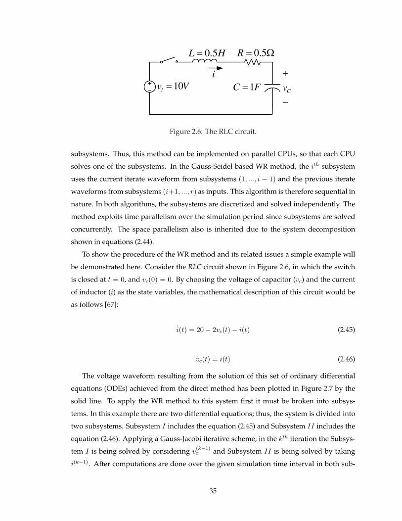
HL 5.0
Vvi
10
5.0R
FC 1Cv
i
Figure 2.6: The RLC circuit.
subsystems. Thus, this method can be implemented on parallel CPUs, so that each CPU
solves one of the subsystems. In the Gauss-Seidel based WR method, the ith subsystem
uses the current iterate waveform from subsystems (1, ..., i − 1) and the previous iterate
waveforms from subsystems (i+1, ..., r) as inputs. This algorithm is therefore sequential in
nature. In both algorithms, the subsystems are discretized and solved independently. The
method exploits time parallelism over the simulation period since subsystems are solved
concurrently. The space parallelism also is inherited due to the system decomposition
shown in equations (2.44).
To show the procedure of the WR method and its related issues a simple example will
be demonstrated here. Consider the RLC circuit shown in Figure 2.6, in which the switch
is closed at t = 0, and vc(0) = 0. By choosing the voltage of capacitor (vc) and the current
of inductor (i) as the state variables, the mathematical description of this circuit would be
as follows [67]:
i(t) = 20− 2vc(t)− i(t) (2.45)
vc(t) = i(t) (2.46)
The voltage waveform resulting from the solution of this set of ordinary differential
equations (ODEs) achieved from the direct method has been plotted in Figure 2.7 by the
solid line. To apply the WR method to this system first it must be broken into subsys-
tems. In this example there are two differential equations; thus, the system is divided into
two subsystems. Subsystem I includes the equation (2.45) and Subsystem II includes the
equation (2.46). Applying a Gauss-Jacobi iterative scheme, in the kth iteration the Subsys-
tem I is being solved by considering v(k−1)c and Subsystem II is being solved by taking
i(k−1). After computations are done over the given simulation time interval in both sub-
35

k=1
k=2 k=6
k=9
k=10
k=13
k=14
k=15
k=21
k=5
Cap
acit
or
Vo
ltag
e (
V)
Time(s)
Figure 2.7: Response of the RLC circuit for the capacitor voltage, k: the number of WRiterations.
systems, waveforms would be exchanged; then, the two subsystems are ready to be solved
for the next iteration with the new waveform data. This procedure will be continued until
the resulting waveforms converge within required accuracy. In Figure 2.7 the response of
several iterations has been superimposed on the direct method response with dash lines.
As k increases, at the end of each iteration the resulting waveform converges toward the
direct method response more than the previous iteration.
From this example one important property of the WR method can be explained. It
can be observed in Figure 2.7 that as the number of iterations increases, the time inter-
val in which the resulting waveform is close to the exact one becomes larger. In other
words, the method works well for a certain interval, but it is inaccurate outside of this
span. So, instead of applying the method in each iteration over the whole simulation time,
it is more effective to divide the simulation time into small intervals (with the length of
win) and solve equations piece by piece within each interval, as shown in Figure 2.8. This
technique, known as windowing, decreases the number of iterations required within each
interval for achieving the certain accuracy [52]. The complete flowchart of WR method
including the windowing technique is depicted in Figure 2.9. Windowing also reduces the
required memory space, because the iterative waveforms need to be stored only for small
time intervals instead of the whole simulation time [67]. In the large-scale networks if the
36

k=1
k=2 k=6
k=9
k=10
k=13
k=14
k=15
k=21
k=5
Cap
acit
or
Vo
ltag
e (
V)
Time(s)
win
Figure 2.8: Application of windowing technique in the WR method, k: the number of WRiterations, win: window length.
intervals are too small, the advantages of the WR method are lost due to the increase in
communication time among the partitions [29].
The same as other parallel computation algorithms, the first requirement in utilizing
the WR method is to partition the problem into smaller tasks that can be distributed among
the several processors. Partitioning can be classified into fine-grain and coarse-grain. In
the former the problem is divided into many small tasks, and consequently, the commu-
nication between the processors is broad. In the later the problem is divided into a few
but large tasks or subsystems which impose less communication on the processors. Thus,
choosing the partitioning approach, is mainly limited by the parallel processor hardware.
If the available hardware cannot provide a fast capability among its processors, the coarse-
grain method is more preferable. A full section discussing this issue appears in the Chapter
3.
2.6 Power System Partitioning
Various approaches based on criteria such as computation loads, network topology, and
dynamic behavior of the system can be used to partition power system for transient sta-
bility simulation. For example the system can be decomposed to split the computation
burden among parallel processors based on the total number of equations, or by consid-
37

Start
Itr = 1
Updating external waveform
variables for all t in win
i = 1 to n
Computing internal
waveform variables in
subsystem # i for win
Waveforms
converge ?
Itr = Itr + 1
NO
Stop
A
B
YES
Itr < MaxItr
NO
YES
win = 1
win = win + 1
win < k
NO
YES
A
Discretization of
differential
equations
Newton-Raphson
Solution of linear
algebraic
equations
B
Figure 2.9: Flowchart of the WR method for the duration of [0, T ] which is divided intok window intervals. n: the total number of subsystems; Itr: counter of iterations in eachwindow; MaxItr: the maximum allowable number of iterations in each window; win:counter for windows.
ering the complexity of the generator models and the connectivity of the buses. There are
methods based on graph theory for network partitioning for use in the block iterative so-
lution of linear systems. In [68] this technique has been used for load flow study in power
systems.
In the approaches that are based on the system dynamics the coherency characteristics
of the generators are used. To find the coherent generators two methods are available. One
is based on time-domain simulation, and the other method is to use eigenvalue analysis.
The best way of determining generator coherency is through observing the swing curves
generated by numerical integration of the system dynamic equations. In a power network
a pair of generators are called coherent if the difference between their rotor angles (δi and
38

δj) remains constant over time:
δi(t)− δj(t) = ∆δij ± ε 0 < t < T (2.47)
where ∆δij is a constant value, and ε is a small positive number. In case that ε = 0
generators i and j are perfectly coherent. However, in the time-domain approach the com-
putation involved for a large-scale system is intensive because it requires solution of the
system dynamic equations. In [70] the time-domain simulation method to find out co-
herent groups of generators has been described based on two assumptions that coherent
generators are independent from the size of disturbance and also the detailed of model-
ing. These assumptions have been validated based on observations of many simulations.
Therefore, a linearized classical model of the synchronous machines can be used to find out
rotor angle trajectories based on criteria in (2.47). Slow coherency partitioning method, re-
ported in [71], has been applied in power systems. In this method instead of time-domain
simulation, the concept of tow-time-scale model is used to decompose the system. Two
time scales related to difference between the inter-area and local oscillations happening
in a power system following a fault. This approach requires the calculation of modes
and eigenvalues of the given system. In [72] a direct method of coherency determination
through the use of Taylor series expansion of the faulted and post faulted systems has
been proposed. There are also methods that decompose the system based on the concept
of the electrical distance between busbars, and is independent of the systems operating
condition [73]. In this thesis the slow coherency method has been used for partitioning
large-scale systems.
2.7 Types of Parallelism Used in This Thesis
We have used three types of parallelism’s:
• Algorithm-level: This is a top-level or coarse-grain parallelism which happens be-
fore any numerical method starts solving the system equations. It is also known as
program-level parallelism [29]. Here the objective is not to address task definition and
scheduling, but the parallelism inherent in the overall algorithm. The WR method is
an example of this type of parallelism.
• Task-level: In this type of parallelism the traditional serial algorithm is converted
into various smaller and independent tasks which may be solved in parallel. For
39

D.P.
A.P.
D.P.
T.P. A.P. : Algorithm-level Parallelism
T.P. : Task-level Parallelism
D.P. : Data Parallelism
(a) (b)
Figure 2.10: Integrating various types of parallelism: (a) algorithm-level method on a data-parallel hardware, (b) task-level method on a data-parallel hardware.
example, to solve a linear set of equations in the form of Ax = b, the task-level par-
allelism entails decomposing the matrix A into various other matrices that can be
solved in parallel. Using the sparsity related solution methods, or converting matrix
A into a block-bordered diagonal matrix are examples of the task-level parallelism
approach. The parallel-in-space methods explained earlier also falls into this cate-
gory.
• Data-parallelism: This is the most fine-grained type of parallelism that can be used on
the SIMD-based architectures such as vector processors or GPUs. A given problem
must have the capability to be expressed in the data-parallel format in order to take
advantages of the SIMD hardware.
Both the algorithm-level and task-level approaches can take advantage of data-parallelism
techniques as shown in Figure 2.10. In Chapter 5 it will be shown how the proposed
algorithm-level parallel method, i.e. Instantaneous Relaxation, and a task-level parallel
method, known as Incomplete LU factorization, can be implemented on data-parallel ar-
chitecture of GPUs.
2.8 Summary
In this chapter the subject of parallel processing based computation applicable for tran-
sient stability simulation of large-scale power systems has been discussed. To this end
we started with the general classification of parallel processors hardware architectures to
describe two state-of-the-art available processor techniques (PC-Cluster based real-time
simulator and GPUs) in the RTX-LAB. The second portion of this chapter was allocated to
the parallel solution methods for the differential-algebraic equations, and approaches spe-
cific to the transient stability simulation of power systems have been discussed. In Chapter
40

3 the general idea of the WR method suitable for real-time simulation is discussed. How-
ever, the original WR method contains drawbacks which offer serious obstacles for imple-
mentation in real-time space. The proposed approach in this thesis is the Instantaneous
Relaxation method that will be comprehensively described in Chapter 3. As the Instan-
taneous Relaxation and WR methods have a common mathematical background, the WR
method was explained with more details in this chapter to prepare the reader for Chapter
3.
41

3The Instantaneous Relaxation (IR) Method
3.1 Introduction
The objective of this chapter 1 is to revisit the application of real-time digital simulators to
the transient stability problem. As mentioned in the previous chapter, transient stability
simulation of realistic-size power systems involves computationally onerous time-domain
solution of thousands of nonlinear differential algebraic equations (DAE’s). Furthermore,
from the point of view of dynamic security assessment which is required for safe system
operation and control, several transient stability cases need to be run in a short period of
time for analyzing multiple contingencies and to initiate preventive control actions.
Currently available commercial real-time simulators such as RTDS [74], RT-LAB from
OPAL-RT Technologies Inc. [51], and Hypersim [75] address these needs to a large extent
by using multiple racks or clusters of multi-processor architectures. The question that
arises, however, is whether this approach is the most efficient and cost-effective, given the
prevalent practice of using a real-time simulator, originally designed and built for electro-
magnetic transient studies, for transient stability simulations. This is done, of course, using
simpler models and larger time-steps. For example, nominal-pi models are used instead of
frequency-dependent models for transmission lines, and the simulator time-step is chosen
to be in the range of milliseconds instead of microseconds. Nevertheless, there is underly-
ing sequentiality in the electromagnetic transient simulation algorithm [76] that precludes1Material from this chapter has been published: V. Jalili-Marandi, V. Dinavahi, “Instantaneous relaxation-
based real-time transient stability simulation,” IEEE Trans. on Power Systems, vol. 24, no. 3, August 2009, pp.1327-1336.
42

an efficient utilization of the hardware capabilities for transient stability simulation. By
exploiting the parallelism inherent in the transient stability problem, a parallel solution
algorithm can be devised to maximize the computational efficiency of the real-time sim-
ulator. This would reduce the cost of the required hardware for a given system size or
increase the size of the simulated system for a fixed cost and hardware configuration.
In this chapter we propose a fully parallel Instantaneous Relaxation (IR) method for real-
time transient stability simulation. The idea of using relaxation-based solution of DAE’s is
certainly not new and has been explored before. The Waveform Relaxation (WR) method,
described in the previous chapter, was first introduced in [62] for VLSI circuit simulation.
Then in [63] this method was applied to the power systems area and used comprehensively
for off-line transient stability simulation [65]. The classical model of the synchronous ma-
chine was used in these simulations. Although this algorithm was implemented sequen-
tially, it was predicted that it will accelerate the simulation by exploiting parallel proces-
sors [29]. Later in [66] the WR method was implemented on parallel computers.
As will be explained later, although the WR method is a parallel method successfully
implemented for off-line simulations, there are inefficiencies that surface when it is im-
plemented in real-time. Therefore, the IR method which overcomes these limitations is
proposed for real-time implementation.
The chapter begins with a discussion about the obstacles of the WR method for real-
time implementation. The algorithm of the proposed IR method will be explained, and
the approach for partitioning a power system for performing IR method will be discussed.
Real-time simulation results and their comparative analysis with off-line simulations will
be shown at the end.
3.2 Limitations of WR method for Real-Time Transient StabilitySimulation
The WR method was explained in the Chapter 2. The most important advantages of this
method as a parallel-processing application where parallelism happens at the program
level and not at the task level, are:
• it is an inherently parallel method.
• multi-rate integration methods can be used.
• each subsystem can be solved independently
43

1
r-1
2 3
r
Figure 3.1: Partitioning a large system into subsystems.
• subsystems become smaller than the original large system, it takes less time to solve.
• different levels of accuracy for modeling in each subsystem can be used.
Figure 3.1 schematically shows a large-scale power system partitioned into r smaller
subsystems to conduct a parallel simulation by using the concept of WR method. The
outstanding difference between the WR and other classical decomposition methods for
solving linear and non-linear algebraic equations is that in this method during each iter-
ation each subsystem is analyzed for the entire time interval [0, T ]. In other words, the
elements in this technique are waveforms of the variables rather than their instantaneous
values. In each iteration of the WR method each subsystem is solved by using the three
basic steps of the transient stability standard approach for all t ∈ [0, T ].
It was discussed in [67] and [29] that the WR method works well for a certain interval,
but it is inaccurate outside of this span. So, instead of applying the method in each iteration
over the whole simulation time, i.e. [0, T ], it is more effective to divide the simulation time
into k small intervals or windows, i.e. [0, T1], [T1, T2],..., [Tk, T ], and solve equations piece
by piece within each interval. This technique, known as windowing, decreases the number
of iterations required within each interval for achieving required accuracy [52]. Further-
more, windowing reduces the required memory space, because the iterative waveforms
need to be stored only for small time intervals instead of the whole simulation time.
44

The waveform-based property of the WR method is one issue that needs to be changed
for real-time simulation. There are two reasons. First, in real-time simulation and specifi-
cally in hardware-in-the-loop simulation the instantaneous value of each variable at each
time-step is required and not the complete waveforms. Second, if waveforms are going
to be used as numerical elements, all waveforms of the variables such as bus voltages or
generator angles must be computed for the entire simulation interval, say 20s, in the first
time-step of the simulation, say 1ms. Clearly, this is not practical for a large-scale system
with thousands of variables. To overcome this restriction the windowing technique can
be used. So, the whole simulation time is divided into small intervals, and each interval
is computed in one time-step. The time intervals must be small enough so that the com-
putation tasks can be performed during one time-step. Although windowing can help
maintain the waveform property; however, working with waveforms in real-time is not as
efficient as in off-line simulation.
Suppose the simulation interval [0, T ]s is divided into k windows of length m× h mil-
liseconds, h being the time-step. When the simulation starts, all waveforms for the interval
of the first window must be computed during the first time-step. Then, there are two op-
tions. In the first option (Figure 3.2) the real-time simulator is idle during the remaining
length of the first window, i.e. for (m− 1)× h milliseconds, when it just sends out instant
values of variables at each time-step. After this period simulator resumes computation for
the interval of the second window, and again becomes idle. This process is repeated until
the end of simulation time. In the second option, depicted in Figure 3.3, the simulator con-
tinues the computation for each window in the subsequent time-steps while it also sends
out the instantaneous values of variables at each time-step. Therefore, the computation fin-
ishes in k consecutive time-steps, and after that the simulator becomes idle when it sends
out instant values at each time-step. It can be concluded that in both options the simulator
performs the entire computation in k time-steps and then remains idle for (m−1)×k time-
steps. In other words, the computation load has not been distributed among the time-steps
equally. Thus, real-time implementation of the native WR method can be inefficient from
resource utilization point of view.
3.3 Instantaneous Relaxation
To overcome the limitations of the WR for real-time implementation we propose the point-
wise or Instantaneous Relaxation (IR) technique. It is simply the WR method with a window
45

Model
time-line
Simulator
time-line
x0
x1
xT
win1
Waveform
calculation
Sending out
instant values
win2
wink
0 T
Idle Idle Idle
h
m
Figure 3.2: Real-time implementation of the WR method: Option 1.
Model
time-line
Simulator
time-line
x0
x1
xT
win1
Waveform
calculation
Sending out
instant values
win2
wink
0 T
Idle
Xk-1
Figure 3.3: Real-time implementation of the WR method: Option 2.
length of one time-step, i.e. m = 1. It has been verified in the off-line implementation
of WR method that the smaller the length of window, the faster the convergence. On
the other hand, if the window is made too small the overall communication time among
subsystems increases which causes a loss of the advantages of the WR method. However,
the communication latency between computation nodes in currently available real-time
simulators is in the order of a few microseconds. This latency is small compared to the
time-step required for transient stability and can therefore be neglected. Based on the
previous experience with the WR method and the arguments made in the pervious section,
it can be concluded that the IR method not only inherits the advantages of the WR method
but is also efficient from the real-time simulation point of view.
To apply relaxation methods at the level of differential equations the preliminary step
is clustering variables into groups which can be solved independently. This will be specifi-
cally discussed for the transient stability application in the next section. After partitioning
the system into n subsystems, the set of DAE’s equations (i.e. (3.1) and (3.2)) are prepared
46

to describe the dynamics of each subsystem:
xint = f(xint,xext,Vint,Vext, t), (3.1)
0 = g(xint,xext,Vint,Vext, t), (3.2)
where xint and Vint are state and algebraic variables that define the dynamic behavior
of Subsystem i, and xext and Vext are the state and algebraic variables that defining all
subsystems excluding Subsystem i. Therefore, x = xint⋃
xext and V = Vint⋃
Vext are
the set of all state and algebraic variables that describe the original-size system. Using the
Gauss-Jacobi iteration scheme the pseudo code for the GJ-IR method is as follows:
guess initial values for xint and Vint at each subsystem
t=0;
repeat{t=t+1;
for each subsystem solve
xintt = f(xint
t ,xextt−1,V
intt ,Vext
t−1)
0 = g(xintt ,xext
t−1,Vintt ,Vext
t−1)
}until (t>T)
and using the Gauss-Seidel iteration scheme the GS-IR method is as follows:
guess initial values for xint and Vint at each subsystem
t=0;
repeat{t=t+1;
for each subsystem solve
xintt = f(xint
t ,xextt ,Vint
t ,Vextt )
0 = g(xintt ,xext
t ,Vintt ,Vext
t )
}until (t>T)
From the above mentioned algorithms, the obvious difference between GJ-IR and GS-
IR is that in the GS-IR at each time-step the Subsystem i has to wait until Subsystems 1 to
i − 1 get solved, so that Subsystem i can use the last values of the xext and Vext to solve
xint and Vint. However, in the GJ-IR the solution of Subsystem i for the current time-step
47

is fully independent from the solution of other subsystems. Therefore, the GS-IR has a
sequential nature while the GJ-IR is fully parallel that makes it suitable for our purpose.
From now on, in this thesis the IR method refers to the GJ-IR.
To solve each subsystem we first start with discretizing (3.1) that results in a new set of
non-linear algebraic equations. In this work we used the trapezoidal rule as the implicit
integration method to discretize the differential equations as follows:
0 = xi − h
2[f i(xi,Vi, t) + f i(xi,Vi, t− h)
], (3.3)
where i = 1, 2,. . . ,n indicates the subsystem, and h is the integration time-step. (3.2)
and (4.4) can be linearized by the Newton-Raphson method (for the jth iteration) as:
J(zij−1) ·∆zi = −Fi(zi
j−1), (3.4)
where J is the Jacobian matrix, zi = [xi,Vi], ∆zi = zij − zi
j−1, and Fi is the vector of
nonlinear function evaluations. (4.5) is a set of linear algebraic equations that can be solved
with Gaussian Elimination and back substitution method. Benchmarking revealed that a
majority of execution time in a transient stability simulation is spent for the nonlinear so-
lution. By using the IR method, however, and by distributing the subsystems over several
parallel processors, a large-scale system is divided into individual subsystems whose ma-
trix sizes are smaller resulting in faster computations.
To clarify the differences between the WR and IR methods, the flowcharts of IR algo-
rithm is shown in Figure 3.4 which can be compared with Figure 2.9 in Chapter 2. Prac-
tically in the WR method it does not seem efficient to perform several iterations of the
Newton-Raphson. Let the exact solution of a waveform be x(.), and the result of the kth
iteration of the WR method be xk(.). Depending on the length of window some iterations
will be required for xk(.) to converge to x(.); however, the starting iterations for xk(.) are
poor approximations of x(.). Thus, it is superfluous to perform Newton-Raphson itera-
tions for computing a close approximation to xk(.) which itself is a poor approximation of
x(.). The convergence rate of the IR method is higher than that of WR, because its win-
dow length is minimum. Therefore, performing several iterations of Newton-Raphson, as
shown in Figure 3.4, increases the accuracy of IR.
Following the convergence of iterative solutions in all subsystems, the state and alge-
braic variables calculated from the last time-step are updated. The state variable descrip-
tion of generators used in this work was defined in Chapter 1. These state variables and
voltages of generator buses must be exchanged between all interconnected subsystems.
48

Start
t = 0
Updating external
instantaneous variables in all
subsystems using Gauss -Jacobi
i = 1 to n
Computing internal
instantaneous variables in
subsystem # i
t < TYes
Stop
A
B
NO
t = t + h
A
Discretization of
differential
equations
Newton-Raphson
Solution of linear
algebraic
equations
B
Converge?
j = 1
j < MaxItr
NO
NO
YES
YES
j = j + 1
Figure 3.4: Flowchart of the proposed IR method for the duration of [0, T ] with a time-stepof h. j: counter for iterations of the Newton-Raphson; MaxItr: the maximum allowablenumber of iterations for the Newton-Raphson in each time-step.
3.4 Coherency Based System Partitioning for the IR Method
One way to partition a power system for parallel processing is to distribute equal numbers
of generators and buses among the processors. However, this is not an efficient method
because the network buses have different connectivity and the generator models vary in
both size and complexity. This gives rise to the load balancing problem in a parallel multi-
processor simulator architecture. Another option is to split the computation burden among
processors based on the total number of equations; however, this approach will increase
both the programming and communication complexity. A more efficient method is to
partition the system by considering the complexity of the generator models and the con-
nectivity of the buses. In this case, different number of generators and buses are assigned
to parallel processors, and the computation burden is roughly even; however, the draw-
49

back of this method is that it cannot be used for a general-purpose program at least in the
off-line sense [77].
The primary requirement for successfully using the relaxation methods at the level of
differential equations is to divide the system into subsystems in which tightly coupled
variables are grouped together. In [52] it was shown that the WR method will converge
for any chosen partitioning scheme; however, the rate of convergence is highly dependent
on the method of partitioning [29]. In spite of all that, it is important to ask this ques-
tion: is transient stability simulation of a large-scale network by IR method restricted by
this prerequisite? In other words, whether the partitioning scheme’s dependence on sys-
tem modeling or the characteristics of the disturbance such as its severity or location, will
influence the convergence of the IR or WR methods.
Determination of tightly coupled variables or simply partitioning the system can find
a physical meaning from the power system point of view. Following a large disturbance in
the system, some generators lose their synchronism with the network. Thus, the system is
naturally partitioned into several areas in which generators are in step together while there
are oscillations among the different areas. Generators in each of these areas are said to be
coherent. The coherency characteristic of the power system reflects the level of dependency
between generators. Coherent generators can be grouped in the same subsystem which
can be solved independently from other subsystems with the WR or IR methods. The
partitioning achieved using the coherency property has two characteristics which make
it appropriate for our study. The coherent groups of generators are independent of: (1)
the size of disturbance and (2) the level of detail used in the generators. Therefore, the
linearized model of the system and the simple classical model of generators can be used
to determine coherency. Furthermore, slow coherency based grouping is insensitive to the
location of disturbance in the power system [78]. These features of slow coherency lead us
to use this partitioning method in this thesis.
3.5 Implementation of IR Method
The IR method was implemented using a customized MATLAB S-function. S-function is
a computer language description of a SIMULINK block that can be written in either C,
C++, Fortran, Ada, or MATLAB, and it is compiled as a mex file to dynamically link into
MATLAB. The most common use of S-function is to create a custom SIMULINK block.
This block may include a new general purpose application, a hardware device driver, or
50

describing a system as a set of mathematical equation. In our case, the purpose was to
implement the IR method. Thus, we use the S-function to mathematically model the power
system equipments and solve it using the proposed IR method.
The customized S-function block is solved at every time-step assigned by SIMULINK
but the time-step can be changed from outside the S-function in the main model. The
change in time-step can be passed to the S-function structure by defining it as a parameter
of the S-function. The ‘discrete solver’ option is used for the simulation, even though
selection of different solver in SIMULINK does not influence the S-function as the solver
is chosen inside the S-function structure. The models developed in SIMULINK could be
solved with either variable or fixed time-step. Due to the model validation process, only
the fixed-step solver was utilized. In this research we used the C programming language
to prepare the SIMULINK S-function which will be explained in this section.
3.5.1 Building of C-based S-Function
The general structure of the S-function written in C is shown in Figure 3.5. The SIMULINK
S-Function block is invoked at each simulation time-step, and any changes in the S-function
inputs can be passed to it even while the simulation is running. As shown in Figure 3.5
flowchart, the essential functions in C-based S-function to be used are the follows.
Function static void mdlInitializeSizes(SimStruct *S)
This is the first invoked function in the S-function, and it is used to specify the basic char-
acteristics of the block, such as number of inputs, outputs, the port width of each input and
output, and the number of parameters of the S-function block. It is worthwhile to mention
that while the simulation is running, the s-function parameters cannot be changed but its
inputs can be changed. In this case, three input and nine output ports are defined. The in-
put corresponds to external machines ID, and variables that are required to be exchanged
among subsystems.
Function static void mdlInitializeSampleTimes(SimStruct *S)
Sample time of the S-function block is initialized here, which is retrieved from the first
S-function parameter by C function mxGetScalar(ssGetSFcnParam(S, 0)).
51

mdlInitializeSizes
mdlInitializeSampleTimes
mdlStart
mdlOutputs
mdlUpdate
mdlTerminate
START
END
DONE? No
Yes
Figure 3.5: SIMULINK S-function flowchart
Function static void mdlStart(SimStruct *S)
All initializations including the network’s steady state parameters, machines data, and
network’s admittance matrix are placed in this function. The data files in the PSS/E *.raw
file format are read and interpreted, and corresponding models are initialized. Moreover,
in order to reduce computational time in the simulation loop, all admittance matrices cor-
responding to the switching states are uploaded here for future access in simulation loop.
Function static void mdlOutputs(SimStruct *S, int T tid)
This is the function invoked in every simulation loop. Outputs requested to be either
monitored, saved, or exchanged between subsystems are sent to S-function block output.
The outputs are calculated in mdlUpdate function discussed below.
52
Function static void mdlUpdate(SimStruct *S, int T tid)
This is the main function implementing all the transient stability numerical calculations.
Invoked in each time step, the function first reads from the S-function block input the
external variables that need to be updated for the current time-step. Then, in case that the
topology of the network has changed, the appropriate admittance matrix will be loaded.
Hereafter, the right hand side of flowchart shown in Figure 3.4 is run. Finally, this function
calculates requested outputs and saves them to be used by the function mdlOutputs for
S-function block output.
Function static void mdlTerminate(SimStruct *S)
In this function, memory blocks allocated for storing transient stability models are freed to
ensure no memory leakage in the C program.
3.5.2 Off-Line Implementation of the IR Method
To implement the IR method, an S-function block that mathematically models power sys-
tem transient stability computations is developed. This is a general block which can
be specified by setting parameters to model a portion of large-scale power system. To
model the complete system, several of these blocks can be simply placed and connected in
SIMULINK environment. Each block represents a subsystem identified by the partitioning
method such as slow coherency method or geographic partitioning. The required parame-
ters of the current version of the developed S-function block are: the numbers of machines
included in the system and in the individual subsystem, the total number of areas, the ID
numbers of internal and external machines. For instance, suppose a power system is de-
composed into three areas each is represented by an S-function block. Figure 3.6 shows the
top lay-out of a three-area system called Area1, Area2, and Area3. Inside the subsystem
Area1 is depicted in Figure 3.7, where the S-function block is identified by area1. This S-
function block involves three input ports, U, I, and IDs, and nine output ports. The output
ports are of two types: the measuring outputs, which are directly sent to the Monitoring
block in Figure 3.6, to be saved or seen on scopes, as illustrated in Figure 3.8, and the data
outputs, which are sent to the external subsystems, i.e. Area2 and Area3, to update them
by the last computations of Area1.
53

measure_a1
measure_a2
measure_a3
Monitoring
data_a1
data_a2
meas ure_a3
data_a3
Area3
data_a1
data_a3
meas ure_a2
data_a2
Area2
data_a2
data_a3
measure_a1
data_a1
Area1
Figure 3.6: Top lay-out of a three-area decomposed system using developed S-functionblocks in SIMULINK for off-line simulation.
3.5.3 Real-time Implementation of the IR Method
The real-time simulation software package provided by OPAL-RT came in the form of
three MATLAB/SIMULINK based toolboxes:
• ARTEMIS: This toolbox provides additional discretization methods, improved solv-
ing algorithms, and a pre-computation mechanism to boost the overall performance
of the SimPowerSystem (SPS) blockset that was built into MATLAB/SIMULINK.
• RT-EVENTS: This toolbox targets specifically the power electronics modeling, oper-
ation, compensation, and optimization.
• RT-LAB: RT-LAB contains the modules that are required for the pre-compilation of
the source code, RT hardware and software interface, and simulation result acquisi-
tion.
The OPAL-RT software package in the RTX-LAB at the University of Alberta requires
two operating systems: Windows XP on the host computers, and RT Linux on the target
nodes. Power system models could be developed off-line in the SIMULINK graphical en-
vironment on the host. In case those models are not available in SIMULINK, user defined
S-function block can also be incorporated into the models (as explained in the previous
54

2
data_a1
1
measure_a1
area1
S-Function1
[I_a2]
[U_a2]
[I_a1]
[U_a1]
[w]
[Te]
[It]
[Vt]
[U]
[IDs]
[I]
[I_a3]
[U_a3]
[IDs_a2]
[IDs_a3]
[IDs_a1]
[Efd]
[delta]
[I]
[U]
[I_a1]
[U_a1]
[w]
[Te]
[It]
[Vt]
[IDs_a3]
[IDs_a2]
[I_a3]
[I_a2]
[U_a3]
[IDs]
[IDs_a1]
[U_a2]
[Efd]
[delta]
2
data_a3
1
data_a2
Figure 3.7: Placing S-function in subsystem Area1 for off-line simulation.
section). When the model optimizations are completed and verified with off-line simu-
lations, the RT-LAB utility is used to transfer the pre-compiled source code into the RT
Linux operating system, which resides on the nodes of the simulator. The execution of
the loaded model could be directly controlled through the Windows based utility without
dealing with the Linux OS.
The target runs on a Linux based real-time operating system which offers optimized
performance through a single programming environment and direct control of all system
operations by using single kernel design. It offers eXtra High Performance (XHP) mode
operation through CPU shielding where one CPU is dedicated for the simulation while
the other CPU is load with RT Linux operation system to manage data feeding to the
shared memory and to interact with the peripheral hardware. The target is responsible for
real-time execution of the model, data transfer between nodes and the host, and data com-
munication with external hardware through I/Os. The target is also required to compile
source code generated by MATLAB/SIMULINK Real-Time Workshop (RTW) to executa-
bles. The hosts are installed with the RT-LAB software provided by Opal-RT Technologies
Inc. to coordinate all hardware engaged for the simulation. The hosts are mainly used to
create, edit and verify models in SIMULINK, compile SIMULINK blocks into C code by
RTW, control and configure real-time simulations in targets, manipulate model parameters
in real time as well as acquire real-time simulation results.
55

w
delta
VT
IT
VT
Efd
DELTA
TE
IT[It_a2]
[Vt_a2]
[Efd_a2]
[delta_a2]
[w_a1]
[Te_a1]
[It_a1]
[It_a3]
[Vt_a1]
[Vt_a3]
[Efd_a3]
[delta_a3]
[w_a3]
[Te_a3]
[a3]
[delta_a1]
[a2]
[w_a2]
[Te_a2]
[Efd_a1]
[a1]
-1
180/pi
[It_a2]
[Vt_a2]
[Efd_a2]
[delta_a2]
[a1]
[Te_a1]
[It_a1]
[w_a3]
[Vt_a1]
[Te_a3]
[It_a3]
[Vt_a3]
[Efd_a3]
[delta_a3]
[a3]
[a2]
[w_a2]
[w_a1]
[Te_a2]
[Efd_a1]
[delta_a1]
Efd
3
measure_a3
2
measure_a2
1
measure_a1
Figure 3.8: Monitoring and saving outputs of the decomposed system.
A view of the real-time simulator target nodes and the host workstation existing in the
RTX-LAB at the University of Alberta is illustrated in Figure 3.9. Each cluster node consists
of a dual Intel XeonTM shared-memory PC running at 3.0GHz on a real-time Linux op-
erating system. The inter-node communication is through InfiniBand with a 10Gb/s data
transferring rate. As shown in this picture, a model, which in our case is a power system,
can be partitioned and distributed among the cluster nodes. In the case of using multiple
nodes, one node is the Master and other nodes operates as Slaves. The name of the master
subsystem, in the top lay-out of the SIMULINK model, must be prefixed with ‘SM’, and
the name of the slave subsystems must be prefixed with ‘SS’. Moreover, the monitoring
block, where the required outputs are being saved and scopes are placed, must be prefixed
by ‘SC’, as shown in Figure 3.10.
Before compiling the SIMULINK model into C-code, the OpComm block from RT-
LAB/OPAL-RT must be added into the subsystems. OpComm is a communication block
that must be used in subsystems receiving signals from other subsystems, all input ports
must go through this communication block being connected, as shown in Figure 3.11.
56

Figure 3.9: Configuration of the PC-cluster based real-time simulator in the RTX-LAB atthe University of Alberta.
3.6 Experimental Results
In this section we will demonstrate results to verify the efficiency of the IR method for
real-time simulation. To do so we have chosen three case studies. One is the Kundur’s
4 machine and 11 bus system found in [9]. The other case study is the IEEE 39 bus New
England test system [80]. There is also a large-scale power system made case study to fully
occupy the computing capacity of the existing real-time simulator. The real-time results
for these case studies have been validated using the PSS/E software program.
To incorporate IR method S-function blocks into RTX-LAB simulator, all the required
*.c and *.h files, as well as the data files must be transferred to targets in RT-LAB for
real-time simulation. Together with existing C code generated by RTW, all the *.c codes
are compiled by GCC/G++ in targets to generate real-time executables. The complete C
source code of S-function program is demonstrated in Appendix A. To compile the source
code into the MEX-function (executable for MATLAB with extension *.dll in Microsoft
Windows platform), the following command is used for all the S-function codes in MAT-
LAB:
57

data_a1
data_a2
meas ure_a3
data_a3
ss_Area3
data_a1
data_a3
meas ure_a2
data_a2
ss_Area2
data_a2
data_a3
measure_a1
data_a1
sm_Area1
measure_a1
measure_a2
measure_a3
sc_Monitoring
Figure 3.10: Top lay-out of a three-area decomposed system using developed S-functionblocks in SIMULINK for real-time simulation.
>> mex -g area1.c
or
>> mex area1.c
The -g option is used to include debugging information in the MEX-function. More
information on debugging SIMULINK S-function is available in [79].
3.6.1 Case Study 1
Figure 3.12 illustrates the test system used as the first case study. Each synchronous gener-
ator is equipped by an exciter and PSS. A set of 6 differential equations model mechanical
rotation, field winding, and 3 damper windings of each synchronous generator as given
in Chapter 2. The complete system can be described by 36 non-linear differential and 8
algebraic equations. Since generators {1, 2} and {3, 4} are coherent, the system can be par-
titioned into two subsystems. This coherency relation can also be observed later in the
simulation results. These two subsystems are distributed across two cluster nodes as seen
in Figure 3.13. The simulation time-step is chosen to be 1ms. Using the IR method, once
the steady-state has been reached, a three-phase fault at Bus 8 is imposed at t = 5s and is
cleared in 80ms. The real-time simulation results are recorded on an external oscilloscope
58

2
data_a1
1
measure_a1
area1
S -F unction1
OpCommTs = 0.001
OpComm
[I_a2]
[U_a2]
[I_a1]
[U_a1]
[w]
[T e]
[It]
[Vt]
[U]
[IDs]
[I]
[I_a3]
[U_a3]
[IDs_a2]
[IDs_a3]
[IDs_a1]
[E fd]
[delta]
[I]
[U]
[I_a1]
[U_a1]
[w]
[T e]
[It]
[Vt]
[IDs_a3]
[IDs_a2]
[I_a3]
[I_a2]
[U_a3]
[IDs]
[IDs_a1]
[U_a2]
[E fd]
[delta]
2
data_a3
1
data_a2
Figure 3.11: Placing S-function in subsystem Area1 for real-time implementation.
2
3
4
56 7 8 9 10
11
Gen2 Gen4
Gen3
C1 C2
Load1 Load2
1Gen1
25km 10km 25km10km110km 110km
Figure 3.12: One-line diagram for Case Study 1.
and saved. The relative machine angles are shown in Figure 3.14 in which Gen4’s angle is
selected as the reference. The real-time results are superimposed on the results found from
PSS/E. As can be seen the IR method is completely stable during the steady-state of the
system, i.e. t < 5sec. During the transient state and also after the fault is cleared, the real-
time results closely follow the results from PSS/E. The maximum discrepancy between
real-time simulation and PSS/E was found to be 0.93%, based on (3.5):
εδ =max|δPSS/E − δIR|
δPSS/E. (3.5)
where δPSS/E and δIR were defined as the relative machine angles from PSS/E and IR
method respectively. It can be further observed from Figure 3.14 that following the fault,
59

G1
G2
Master Subsystem
G3
G4
Slave Subsystem
FP
GA
I/O
Card
In
fin
iBa
nd
Lin
k
Oscilloscope
Figure 3.13: Distribution of subsystems of Case Study 1 among cluster nodes of the real-time simulator.
the oscillations of Gen4 are closer to the oscillations of Gen3 rather than to those of Gen1 or
Gen2. If the reference generator is switched to Gen1 or Gen2 instead of Gen4, it was found
that the oscillations of Gen1 are closer to the oscillations of Gen2 rather than to those of
Gen3 or Gen4. This observation practically demonstrates the coherency relation existing
in this system.
To investigate the effect of the fault location and the partitioning scheme on the per-
formance of the IR method, the following scenario was simulated. Suppose that the fault
happens at Bus 5. Two different patterns of partitioning have been applied for this case.
The first is based on the coherency property of the system, i.e. {1, 2} and {3, 4}. The second
pattern is based on the fact that since G1 is the closest generator to the fault location it will
accelerate faster than other generators in the system; therefore, the system is divided into
two subsystems: {1} and {2, 3, 4}. These two patterns have been simulated in real-time
using the IR method, and then the results were compared with those of PSS/E. Results of
both patterns are close to those from PSS/E, but the maximum error in the second pattern
is larger than the maximum error when coherency-based partitioning was used. Several
other combinations of fault location and partitioning patterns have also been examined in
this system, and it was concluded that slow coherency partitioning based IR method are
the closest to the PSS/E’s results.
Table 3.1 shows the timing performance of Master and Slave nodes of the real-time
simulator running under the XHP execution mode during one time-step (1ms). This table
shows that the tasks of computation and communication are done in less than 60µs. These
60

0 5 10 155
10
15
20
25
30
35
40
45
Time (sec)
Rela
tiv
e m
ach
ine a
ng
les (
deg
rees)
1,4
2,4
3,4
Real-time
PSS/E
Figure 3.14: Comparison of relative machine angles collected from real-time simulator andPSS/E simulation for Case Study 1: δi,4 = δi − δ4; i = 1, 2, 3.
Table 3.1: Performance log for real-time simulation of Case Study 1Duration (µs)
Task Master SlaveComputation 47.91 47.20Communication 11.55 8.12Idle Time 939.45 940.07Other 1.09 4.61Total Step Size 1000 1000
execution times were sampled across many time-steps, and it was found that the idle times
of the processors were uniform throughout those time-steps.
3.6.2 Case Study 2
The one-line diagram of IEEE’s New England test system is shown in Figure 3.15. As in the
previous case study, all generator models are detailed and equipped with AVR and PSS.
The system data in PSS/E format is given in Appendix E. Using the partitioning pattern
mentioned in [80], the system has been divided into 3 subsystems: {1, 8, 9}, {2, 3, 4, 5, 6, 7},
and {10}. These 3 subsystems were distributed on three cluster nodes of the real-time sim-
ulator: one Master and two Slaves, as illustrated in Figure 3.16. A question which may
arise here is about the uneven loading of CPUs. Although it is possible to add {10} to sub-
61

30
2
1
25
37
18
3
4
5
7
8
9
6
31
39 14
15
16
1727
26 28
21
22
24
11
10
32
13
12
23
29
38
35
3620
34
19
33
Gen1
Gen8 Gen9
Gen6
Gen7
Gen4Gen5Gen3
Gen2
Gen10
Load
Generator
Transformer
Figure 3.15: One-line diagram for Case Study 2.
system 1 and to use only 2 computation nodes, our intent in this study was to demonstrate
the implementation of IR in three parallel cluster nodes. Several fault locations have been
tested and the results were compared with those of PSS/E; in all cases results from the IR
method match very well. In this section a sample of these results are presented. A three-
phase fault happens at Bus 21, at t = 1s and it is cleared after 100ms. Gen10 is the reference
generator and the relative machine angles are shown in Figure 3.17 and Figure 3.18. The
maximum deviation of IR real-time simulation result from the PSS/E result based on (3.5)
is 1.51%.
Table 3.2 shows the timing performance of Master and two Slave nodes in the real-
time simulation during one time-step (1ms). Again the sampled idle times were found
to be uniform across several time-steps. In the PC-cluster architecture the Master node is
responsible for communicating with the host computer and also for organizing the com-
munication among the Slaves. This explains why the Master’s communication time in
Tables 3.1 and 3.2 is larger than Slaves’ communication time. Moreover, it can be seen that
the computation time in both case studies is not very high, since the computation load is
distributed equally among all time-steps. From the idle time duration in both Tables it is
62

Master Subsystem
FP
GA
I/O
Ca
rd
In
fin
iBan
d L
ink
Oscilloscope
Slave Subsystem 2
Sla
ve
Subsy
stem
1
G10
G2 G3 G4
G5 G6 G7
G1 G8 G9
Figure 3.16: Distribution of subsystems of the Case Study 2 among cluster nodes of thereal-time simulator.
Table 3.2: Performance log for real-time simulation of Case Study 2Duration (µs)
Task Master Slave1 Slave2Computation 212.77 348.13 17.27Communication 13.44 7.30 4.51Idle Time 770.93 631.73 974.12Other 2.86 12.84 4.1Total Step Size 1000 1000 1000
concluded that larger subsystems can be implemented on each node, and that faster than
real-time simulation is also possible.
The accuracy of the IR method is analyzed by varying the time-step and calculating
the error in (4.24). The results are presented in Table 3.3. As expected when the time-
step increases the computation error increases as well. Nevertheless, it can be predicted
that with larger time-steps larger systems can be simulated on this hardware using the IR
method. It can however be seen that the maximum error depends not only on the time-
step but also on the size of the system. For instance, the time-step of 5ms results in the
maximum error of 1.32% and 3.29% in the 4 and 10 generator systems, respectively.
63

0 5 10 15-10
0
10
20
30
40
50
60
70
80
90
Time (sec)
Rela
tiv
e m
ach
ine a
ng
les (
deg
rees)
5,10
4,10
3,10
2,10
1,10
Real-time
PSS/E
Figure 3.17: Comparison of relative machine angles collected from real-time simulator andPSS/E simulation for Case Study 2: δi,10 = δi − δ10; i = 1 . . . 5.
Table 3.3: Relation between time-step and accuracy of the IR methodMaximum error εδ%
Time-Step (ms) Case study 1 Case study 21 0.93 1.512 1.04 1.705 1.32 3.29
10 1.88 4.2
3.6.3 Case Study 3: Large-Scale System
In the previous two case studies it was concluded that larger subsystems can be imple-
mented on each node of the real-time simulator. By performing several tests with various
sizes of power systems it was realized that each target node of the existing simulator can
be filled with 10 generators all modeled in detailed while still running in real-time with
a time-step of 4ms. As we have 8 target nodes available, the largest system that can be
modeled in real-time is an 80 generators system. This system was made by expanding
the IEEE test system. For this purpose, the IEEE 39 bus system was duplicated 8 times in
the PSS/E software environment, and then interconnected by transmission lines to build
a large-scale network. The result is a 312 bus and 80 generator power system. The steady-
state and dynamic stability of this system has been examined and verified in PSS/E. This
64

0 5 10 15
30
40
50
60
70
80
Time (sec)
Rela
tiv
e m
ach
ine a
ng
les (
deg
rees)
6,10
8,10
9,10
7,10
Real-time
PSS/E
Figure 3.18: Comparison of relative machine angles collected from real-time simulator andPSS/E simulation for Case Study 2: δi,10 = δi − δ10; i = 6 . . . 9.
system was partitioned and distributed in all 8 target nodes of the simulator running in
parallel and in XHP mode. Figure 3.19 illustrates the top lay-out of this system in the
SIMULINK environment prepared to be run on the real-time simulator. As explained in
the previous section one target node must be the master while others are slave nodes (i.e.
7 nodes in this case). The performance log of this simulation is shown in the Appendix
B for randomly selected five successive time steps. These results are directly reported by
MonitoringViewer feature of the RT-LAB software that shows in detailed the timing of
each operation in each target node during the simulation period. For each target node,
this report includes an item called Number of Overruns which counts the number of
time steps that for any reason the simulation could not satisfy the real-time requirements
and lasted more than the fixed time-step. In Appendix B the report includes the timing of
just two nodes: master (sm area1), and one of the slaves (ss area2). The report declares
that the number of overruns for all nodes is 0, which means the simulation was performed
successfully in real-time.
3.7 Summary
This chapter presented a parallel processing method known as instantaneous relaxation
(IR) for the real-time transient stability simulation of large-scale power systems. Although
65

it is possible to utilize real-time simulators based on the electromagnetic transient simula-
tion approach to perform transient stability analysis, the size and cost of the simulator is
usually prohibitive especially for simulating large-scale systems. The motivation behind
this work is to test the real-time feasibility of a fully parallel method that could alleviate
these limitations. The waveform relaxation (WR) method was investigated in this chap-
ter for implementation in real-time. However, it was found that WR method has some
restrictions for real-time simulation due to the following reasons:
• The WR method provides a set of values in the form of a complete waveform. How-
ever, real-time simulation especially hardware-in-the-loop simulation requires in-
stantaneous values of variables.
• Implementation of the WR causes uneven computation loads among the time-steps.
This results in execution time overrun in some time-steps and excessive idling time
in the others. An overrun, which describes a situation when the simulator requires a
larger time-step than the specified fixed time-step to finish its task, is not acceptable
in hard real-time systems.
These problems are overcome by the proposed IR method. It inherits all the advantages of
the WR method but is also efficient for real-time implementation. The two main differences
between the IR and WR methods are:
• In the IR method the instantaneous values of the variables are being used and not
their waveforms.
• To achieve the required accuracy several iterations of the Newton-Raphson within
each time-step are performed.
To demonstrate the performance of the IR method, three case studies have been im-
plemented on a PC-Cluster based real-time simulator and the results are validated by
the PSS/E software. Several comparisons verified the accuracy and efficiency of the IR
method. In addition, the performance of the slow coherency method as the partitioning
tool was analyzed, and it was concluded that for different fault locations in the system
results derived from this method had lower amounts of error.
66

Figure 3.19: Implementation of a large-scale power system for parallel real-time simulationusing the IR method.
67

Part II
Large-Scale Transient StabilitySimulation on GPU-based Hardware
68

4Single GPU Implementation: Data-Parallel
Techniques
4.1 Introduction
Part I of this thesis discussed the real-time simulation of transient stability. The Instan-
taneous Relaxation method was proposed and successfully implemented on the real-time
simulator. It was mentioned that since decades ago several approaches have been devel-
oped to perform transient stability simulation faster for large-scale systems on parallel
computing hardware [49]. We categorized these methods into two major groups: tearing
and relaxation [81]. The commonality of these methods is task-parallelism which executes
the component subsystems on parallel and distributed hardware composed of clusters of
CPUs. Nevertheless, there are two limitations in these methods that contribute to the speed
bottleneck: (1) data-sequential computation on the CPUs of the cluster, and (2) limited data
bandwidth, and latency of the inter-processor communication channels of the cluster.
Recently, the Graphics Processing Unit (GPU), as introduced in Chapter 2, has revealed
the potential to revolutionize state-of-the-art research in data-parallel computing. A data-
parallel application consists of large streams of data elements in the form of matrices and
vectors that have identical computation codes (kernels) applied to them. The data-parallel
characteristic of the GPU gives it a single-instruction-multiple-data (SIMD) architecture.
In Part II of this thesis, i.e. this chapter1 and the next one, we will discuss GPU-based
1Material from this chapter has been published: V. Jalili-Marandi, V. Dinavahi, “SIMD-based large-scaletransient stability simulation on the graphics processing unit,” IEEE Trans. on Power Systems, pp. 1-10, 2010.
69

transient stability simulation for large-scale power systems. The motivation for this work
is twofold: the mathematical complexity along with the large data-crunching need in this
simulation, and the substantial opportunity to exploit parallelism. Both these character-
istics are uniquely suited to the GPU. However, since the GPU’s architecture is markedly
different from that of a conventional CPU, it requires a completely different algorithmic
approach for implementation. The GPU thrives on applications that have a large compu-
tational requirement, and where data-parallelism can be exploited. Therefore any com-
putation that is desired to be implemented on the GPU must be in the SIMD format, oth-
erwise the GPU cannot deliver its computational benefits. Here we propose SIMD-based
programming models to exploit the GPU’s resources for transient stability simulation.
4.2 GPU Overview
As GPU and its applications are new topics in the Power and Energy Society (PES), before
going further into GPU’s application for transient stability simulation, it is important to
first become familiar with GPU’s architecture and programming paradigm.
4.2.1 GPU Evolution
The earliest ancestors of the dedicated graphics processors were originally designed to
accelerate the visualization tasks in the research labs and flight simulators. Later they
found their way to commercial workstations, personal computers, and entertainment con-
sols [82]. By the end of 2000s, the PC add-in graphics cards were developed as fixed-
function accelerators for graphical processing operations (such as geometry processing,
rasterization, fragment processing, and frame buffer processing). Around this time, the
term of “graphics processing unit” (GPU) arose to refer to this hardware used for graphics
acceleration [83].
In the early 2000’s the GPU was a fixed-function accelerator originally developed to
meet the needs for fast graphics in the video game and animation industries [82]. The
demand to render more realistic and stylized images in these applications increased with
time. The existing obstacle in the fixed-function GPU was the lack of generality to ex-
press complicated graphical operations such as shading and lighting that are imperative
for producing high quality visualizations. The answer to this problem was to replace the
fixed-function operations with user-specified functions. Developers, therefore, focused on
improving both the application programming interface (API) as well as the GPU hardware.
70

The result of this evolution is a powerful programmable processor with enormous arith-
metic capability which could be exploited not only for graphics applications but also for
general purpose computing (GPGPU). Taking advantage of the GPUs’ massively parallel
architecture, the GPGPU applications quickly mushroomed to include intensive computa-
tions such as those in molecular biology, image and video processing, n-body simulations,
large-scale database management, and financial services [83].
The especial architecture of the GPU, explained in this section, made it a successful ac-
celerator/processor in particular applications in which a large amount of computations is
required to be performed on a data-parallel structure of input elements, the same as graph-
ics applications. A data-parallel application consists of large streams of data elements in
the form of matrices and vectors that identical computation codes (kernels) are applied
to them. Moreover, the data communication required to compute the output streams is
small. Through the GPUs evolution, as their main duty was for different application de-
mands than the CPU, the architecture of the GPU has progressed in a different direction
than that of the CPU. A life-like rendering of images requires billions of pixels per second
and each pixel requires hundreds or more operations. Therefore, the fundamental design
of the GPU is in such a way to deliver an enormous amount of computations for its best
efficiency in a massive data-parallel application. Later it will be observed that the size of
computation is a key-point to achieve maximum efficiency in a GPGPU application.
4.2.2 GPU Hardware Architecture
To efficiently use and program a GPU it is instructive to learn the GPU’s internal architec-
ture. In this work we have used NVIDIA’s GeForce GTX 200 series. The following section
briefly explains the architecture and hardware specifications that we require for program-
ming purposes.
Figure 4.1 illustrates the architecture of the GPU [84] plugged into the motherboard of
a 2.5GHz quad-core AMD Phenom CPU supported by 4GB of RAM. The GPU accesses
the main memory of the system, i.e. RAM, via the PCIe 2.0 bus (Peripheral Component
Interconnect Express). This version of GPU has 16 links in its PCIe interface that each link
has a bandwidth capability f 0.5GB/s in each direction simultaneously. Thus, the PCIe 2.0
bus shown in Figure 4.1 supports up to 8GB/s transfer rate. This rate between the CPU
and RAM is typically in the 12GB/s range. The GPU runs its own specified instructions
independently but it is controlled by the CPU. The computing element in the GPU is called
a thread. When a GPU instruction is invoked, blocks of threads (with the maximum size of
71

Figure 4.1: Hardware architecture of GPU mounted on the PC motherboard.
512 threads per block) are defined to assign one thread to each data element. All threads
in one block run the same instruction on one streaming multiprocessor (SM).
Each SM includes 8 stream processor (SP) cores, an instruction unit, and on-chip mem-
ory that comes in three types: registers, shared memory, and cache. Threads in each block
have access to the shared memory in the SM, as well as to a global memory in the GPU.
Unlike a CPU, the architecture of the GPU is developed in such a way that more transis-
tors are devoted to data processing rather than data caching and flow control. When a
SM is assigned to execute one or more thread blocks, the instruction unit splits and cre-
ates groups of parallel threads called warps. The threads in one warp are managed and
processed concurrently on the eight stream processors.
The target GPU specifications in this study are given in Tables 4.1. Threads are assigned
by the thread scheduler which talks directly to each SM through a dedicated instruction
unit which in turn assigns the tasks to the eight stream processors. Depending on the GPU
model, 2 or 3 SM’s can be clustered to build a thread processing cluster (TPC). Moreover
two special function units (SFUs) have been included in each SM to execute transcenden-
tal calculations (e.g. sin, cosine), attribute interpolation and for executing floating point
instructions. Figure 4.2 illustrates these units schematically.
72
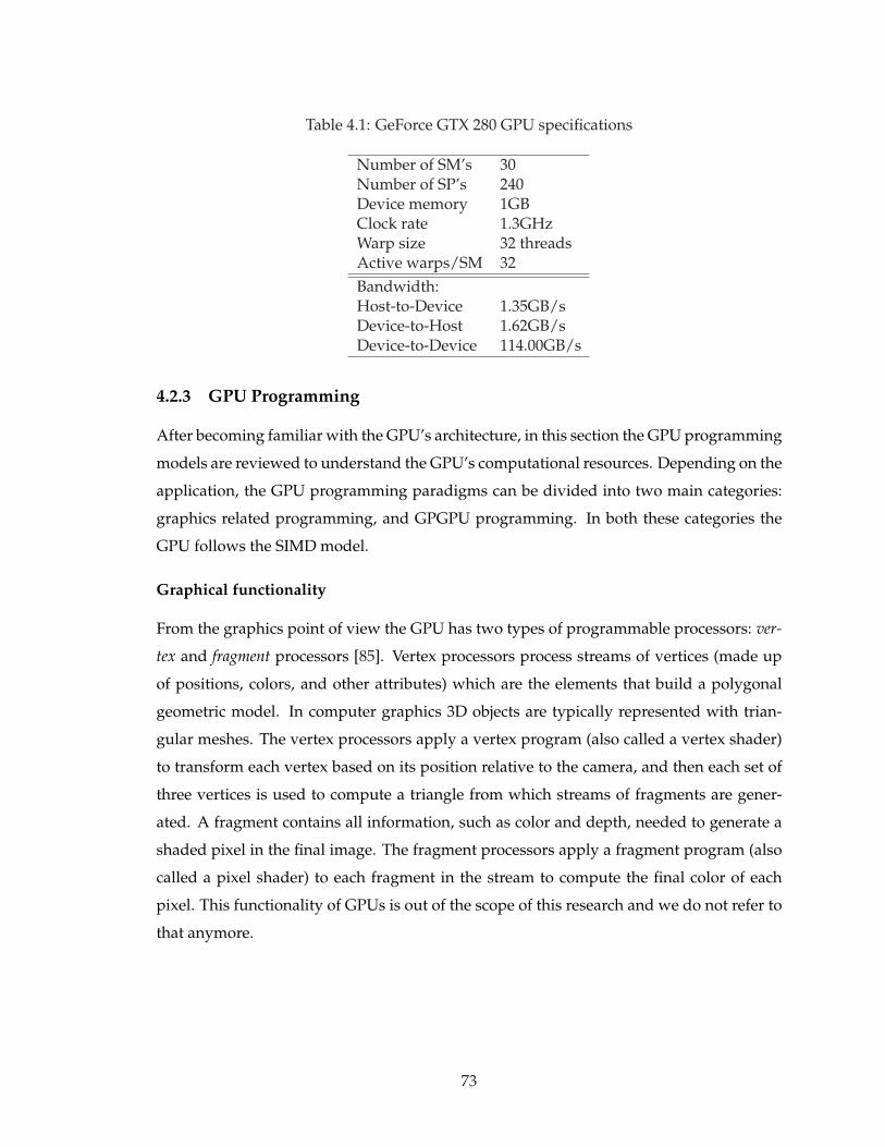
Table 4.1: GeForce GTX 280 GPU specifications
Number of SM’s 30Number of SP’s 240Device memory 1GBClock rate 1.3GHzWarp size 32 threadsActive warps/SM 32Bandwidth:Host-to-Device 1.35GB/sDevice-to-Host 1.62GB/sDevice-to-Device 114.00GB/s
4.2.3 GPU Programming
After becoming familiar with the GPU’s architecture, in this section the GPU programming
models are reviewed to understand the GPU’s computational resources. Depending on the
application, the GPU programming paradigms can be divided into two main categories:
graphics related programming, and GPGPU programming. In both these categories the
GPU follows the SIMD model.
Graphical functionality
From the graphics point of view the GPU has two types of programmable processors: ver-
tex and fragment processors [85]. Vertex processors process streams of vertices (made up
of positions, colors, and other attributes) which are the elements that build a polygonal
geometric model. In computer graphics 3D objects are typically represented with trian-
gular meshes. The vertex processors apply a vertex program (also called a vertex shader)
to transform each vertex based on its position relative to the camera, and then each set of
three vertices is used to compute a triangle from which streams of fragments are gener-
ated. A fragment contains all information, such as color and depth, needed to generate a
shaded pixel in the final image. The fragment processors apply a fragment program (also
called a pixel shader) to each fragment in the stream to compute the final color of each
pixel. This functionality of GPUs is out of the scope of this research and we do not refer to
that anymore.
73

SM
SP SP
Cache
SP SP
SP SP
SP SP
SFU SFU
Memory
SM
SP SP
Cache
SP SP
SP SP
SP SP
SFU SFU
Memory
SM
SP SP
Cache
SP SP
SP SP
SP SP
SFU SFU
Memory
TPC SM
SP SP
Cache
SP SP
SP SP
SP SP
SFU SFU
Memory
SM
SP SP
Cache
SP SP
SP SP
SP SP
SFU SFU
Memory
SM
SP SP
Cache
SP SP
SP SP
SP SP
SFU SFU
Memory
TPC SM
SP SP
Cache
SP SP
SP SP
SP SP
SFU SFU
Memory
SM
SP SP
Cache
SP SP
SP SP
SP SP
SFU SFU
Memory
SM
SP SP
Cache
SP SP
SP SP
SP SP
SFU SFU
Memory
TPC SM
SP SP
Cache
SP SP
SP SP
SP SP
SFU SFU
Memory
SM
SP SP
Cache
SP SP
SP SP
SP SP
SFU SFU
Memory
SM
SP SP
Cache
SP SP
SP SP
SP SP
SFU SFU
Memory
TPC SM
SP SP
Cache
SP SP
SP SP
SP SP
SFU SFU
Memory
SM
SP SP
Cache
SP SP
SP SP
SP SP
SFU SFU
Memory
SM
SP SP
Cache
SP SP
SP SP
SP SP
SFU SFU
Memory
TPC
Thread Scheduler
SM
SP SP
Cache
SP SP
SP SP
SP SP
SFU SFU
Memory
SM
SP SP
Cache
SP SP
SP SP
SP SP
SFU SFU
Memory
SM
SP SP
Cache
SP SP
SP SP
SP SP
SFU SFU
Memory
TPC SM
SP SP
Cache
SP SP
SP SP
SP SP
SFU SFU
Memory
SM
SP SP
Cache
SP SP
SP SP
SP SP
SFU SFU
Memory
SM
SP SP
Cache
SP SP
SP SP
SP SP
SFU SFU
Memory
TPC SM
SP SP
Cache
SP SP
SP SP
SP SP
SFU SFU
Memory
SM
SP SP
Cache
SP SP
SP SP
SP SP
SFU SFU
Memory
SM
SP SP
Cache
SP SP
SP SP
SP SP
SFU SFU
Memory
TPC SM
SP SP
Cache
SP SP
SP SP
SP SP
SFU SFU
Memory
SM
SP SP
Cache
SP SP
SP SP
SP SP
SFU SFU
Memory
SM
SP SP
Cache
SP SP
SP SP
SP SP
SFU SFU
Memory
TPC SM
SP SP
Cache
SP SP
SP SP
SP SP
SFU SFU
Memory
SM
SP SP
Cache
SP SP
SP SP
SP SP
SFU SFU
Memory
SM
SP SP
Cache
SP SP
SP SP
SP SP
SFU SFU
Memory
TPC
Figure 4.2: The GTX 280 hardware architecture: it consists of 10 TPCs, 3 SMs per TPC,and a total of 240 SPs; TPC: thread processing cluster, SM: streaming multiprocessor, SP:stream processor.
General purpose functionality
Early GPGPU programming directly used the existing graphics API’s to express computa-
tions in terms of an image. In other words, the computational elements (i.e. vectors and
matrices) were mapped onto the graphical elements (i.e. vertices or pixels) which are the
components of shading programs. Shading languages used for this purpose include Cg,
HLSL, and OpenGL. Although this technique has been successfully used in many research
areas, including power system load flow computations [86], it was largely unapproachable
by the common programmer. Firstly, because there is a mismatch between traditional pro-
gramming and the graphics API’s, and secondly, because it is difficult to debug or modify
these programs.
High level programming languages
Along with the evolution of the programmable GPU’s hardware architecture, the devel-
opers designed higher level languages that were specifically for general computation pur-
poses. Dedicated GPU programming tools that bypassed the graphics functions of the
GPU were created for general purpose computing, starting with Brook and Sh, and ulti-
mately leading to commercial tools such as AMD’s HAL and NVIDIA’s CUDA.
CUDA (Compute Unified Device Architecture) provides a C-like syntax to execute and
manage computations on the GPU as a data-parallel computing device. A CUDA program
consists of multiple phases that are executed on either the CPU (host) or the GPU (device).
74

The phases of the program that exhibit little or no data-parallelism are run in the host-
code after compiling with the host’s standard C compiler, whereas the phases that exhibit
fine-grained parallelism are implemented in the device-code in the form of kernels, the syn-
onym for GPU functions. Host-code uses a CUDA-specific function-call syntax to invoke
the kernel code. Calling a kernel distributes the tasks among the available multiprocessors
to be simultaneously run on a large number of parallel threads. The programmer orga-
nizes these threads into a grid of thread blocks. Thread creation, scheduling, and resource
management are performed in hardware. Each thread of a CUDA program is mapped to a
physical thread resident in the GPU, and each running thread block is physically resident
on a SM.
Moreover, a library of the basic linear algebra subprograms (BLAS) is provided that
allows the integration with C++ code. By using this library, called CUBLAS, portions of a
sequential C++ program can be executed in SIMD-form on the GPU, as shown in Figure
4.3, while other parts of the code are executed sequentially on the CPU [87]. Wherever a
kernel is invoked a grid consisting of several blocks with equal numbers of threads/block
is created. Each block within a grid, and each thread within a block are identified by in-
dividual indices that make them accessible via the built-in variables in CUDA. Threads
determine the task they must do and the data they will access by inspecting their own
thread and block IDs. Therefore in an application with highly intensive computations,
the onerous computation tasks can be offloaded to the GPU, and performed faster in par-
allel, whereas mundane tasks such as the flow control of the program, required initial
calculations, or the updating and saving of the variables can be done by the CPU. This
co-processing configures a hybrid GPU-CPU simulator.
4.3 Data-Parallel Computing
Here the fundamental difference in the computing model of a GPU and a CPU is discussed,
which leads us to a new methodology to implement the transient stability simulation on
the data-parallel architecture of GPU. From the programmer’s perspective a GPU is a par-
allel machine, whereas the CPU is a serial machine. A CPU executes one instruction after
the another, and each instruction does one thing, for instance, adding the contents of two
memory locations. A GPU, on the other hand, can add many pairs of numbers at the same
time.
Let us look at a simple example. Suppose we want to evaluate z = x + y, where x, y,
75

CUDA Program
C/C++ Code
CUDA kernels
or
CUBLAS functions
C/C++ Code
CUDA kernels
or
CUBLAS functions
Seq
uen
tiali
ty i
n t
he p
rogram
Host (CPU)
Runs sequentially
Host (CPU)
Runs sequentially
Device (GPU)
Grid 0
Runs in parallel
Device (GPU)
Grid 1
Runs in parallel
Grid 0 (i blocks, n threads/block)
block 0
thread
0
thread
1
thread
n
block 1
thread
0
thread
1
thread
n
block i
thread
0
thread
1
thread
n
Grid 1 (j blocks, m threads/block)
block 0
thread
0
thread
1
thread
m
block 1
thread
0
thread
1
thread
m
block j
thread
0
thread
1
thread
m
Figure 4.3: Cooperation of the host and device to execute a CUDA program, and the hier-archy of computing structure in a GPU.
and z are n× 1 real vectors. On the CPU, a single for loop is typically used over all array
elements as follows:
for(i = 0; i < n; i + +)
z[i] ← x[i] + y[i]
In this model two levels of computation are active: outside the loop, the loop counter i
is increasing and compared with the length of vectors n, whereas inside the loop, the arrays
are accessed at a fixed position determined by the loop counter and the actual computation
is performed (addition on each data element). The calculations performed on each data
element in the vectors are independent of each other, i.e., for a given output position,
distinct input memory locations are accessed and there are no data dependencies between
elements in the result vector.
If we had a vector processor capable of performing operations on whole vectors of
length n or even n CPUs, we would not need the for loop at all. This is the core idea
of SIMD programming. The computation on the GPU is performed by separating the
outer loop from the inner calculations. The inner loop calculations are extracted into a
computational kernel as follows:
if(index < n)
z[index] ← x[index] + y[index]
where index is the ID of the threads assigned to elements of the vectors. Note that the
kernel is no longer a vector expression but a scalar template of the underlying math that
76

forms a single output value from a set of input values. For a single output element, there
are no data dependencies with other output elements, and all dependencies to input ele-
ments can be described relatively. Whenever a kernel is called, the driver logic hardware
schedules each data item into the different multiprocessors (SM)–this is not programmable.
Although internally the computation is split up among the available SMs, one cannot con-
trol the order in which they are working. One can therefore assume that all work is done
in parallel without any data interdependence.
Here is a simple example to show how a CUDA-based SIMD kernel looks like. Suppose
we want to model a limiter to control the maximum and minimum amounts of a signal as
shown in Figure 4.4. In the transient stability simulation of power systems these limiters
are widely used in the model of excitation and PSS devices for synchronous generators,
and depending on specifications of each machine the up and down limits are different.
Suppose the output signals of the transfer function that we want to pass them through the
limiter are saved in a vector, V2. We also need two vectors whose elements are the maxi-
mum and minimum limits of the signals at each individual machine, i.e. vmax and vmin.
The implementation of this model by using the function concepts in C++ running sequen-
tially on the CPU is as follows:
void
limiterFunc(float* V in, float* V max, float* V min,const int numElems)
{for (int i=0; i < numElems; i++)
{if (V in[i] >= V max[i])
V in[i] = V max[i];
else if (V in[i] < V min[i])
V in[i] = V min[i];
}}
where in this code V in is the vector of input signals, i.e. V2 in Figure 4.4, V max and
V min are the maximum and minimum limits of each limiter, and numElems is the length
of the input signal. The porting of this function in CUDA language running in SIMD
format on the GPU is a kernel as below:
77

maxv
minv
Transfer
Function 3V1V 2V
Figure 4.4: An schematic model for a limiter.
global void
limiterKernel(float* DEVICE1, float* DEVICE2, float* DEVICE3,const int numElems)
{int idx = threadIdx.x + blockDim.x * blockIdx.x;
if (idx < numElems)
{if (DEVICE1[idx] >= DEVICE2[idx])
DEVICE1[idx] = DEVICE2[idx];
else if (DEVICE1[idx] < DEVICE3[idx])
DEVICE1[idx] = DEVICE3[idx];
}}
In this kernel the global qualifier in the first line declares a function as being a ker-
nel. Such a function is callable from the CPU and is executed on GPU. The up and down
limits for each limiter are saved and transferred to the GPU in two vectors: DEVICE2
and DEVICE3. The values of input signal, which also has been transferred to GPU, i.e.
DEVICE1, is compared with these limits to meet the required conditions. We can see in
this kernel there is not any for loop, and instead of that a new parameter, called idx, is
defined to control the execution of the kernel. To invoke this kernel from a CPU-based
code we need to add a syntax as below:
limiterKernel<<<dimGrid, dimBlock>>>(DEVICE1, DEVICE2, DEVICE3, N);
where the first parameter of the <<< ... >>> specifies the dimension of the grid, and the
second parameter defines the size of the thread block. The index of each block within the
grid and its dimension are identified and accessible within the kernel through the built-in
78

variables, i.e. blockIdx and bloclDim respectively. Each thread inside the thread block
is also identified by a built-in index called threadIdx. Therefore, each thread in the grid
can be addressed by an index calculated based on these built-in variables. This is what the
parameter idx does in the limiterKernel code. Comparing idx and the length of the
vectors specifies the number of required active threads and controls running the code.
4.4 SIMD-Based Standard Transient Stability Simulation on theGPU
4.4.1 Standard Transient Stability Simulation
The general form of DAEs which describe the dynamics of a multi-machine power system
discussed in Chapter 2 are repeating here for easy referencing:
x = f(x,V, t) (4.1)
0 = g(x,V, t) (4.2)
x(t0) = x0 (4.3)
where x is the vector of state variables, x0 is the initial values of state variables, and V
is the vector of bus voltages. The standard approach to solve these nonlinear and coupled
DAEs involves three steps [12]:
• Step 1. The continuous-time differential equations are first discretized and con-
verted to discrete-time algebraic equations. Using an implicit numerical integration
method, discretizing (4.1) results in a new set of non-linear algebraic equations:
0 =h
2[f(x,V, t) + f(x,V, t− h)]− (x(t)− x(t− h)) (4.4)
where h is the integration time-step.
• Step 2. The existing non-linear algebraic equations are linearized by the Newton-
Raphson method (for the jth iteration) as:
J(zj−1) ·∆z = −F(zj−1) (4.5)
where J is the Jacobian matrix, z = [x,V], ∆z = zj − zj−1, and F is the vector of
nonlinear function evaluations.
79

• Step 3: The resulting linear algebraic equations are solved to obtain the system state.
(4.5) is solved using the LU factorization followed by the forward-backward substi-
tution method.
Chapter 2 describes how to solve the network equations.
4.4.2 SIMD Formulation for Transient Stability Solution
The CPU and the GPU have radically different architectures, so they require different pro-
gramming approaches. The generator and the network model shown in Chapter 2 are
suitable for sequential computation on the CPU. To be able to perform these computations
on the GPU, the equations must be expressed in the SIMD format, i.e. instead of using
single-element values vectors or matrices of them must be used. This is straightforward
for the generator equations and is accomplished by replacing all variables and parameters
with the vectors whose elements relate to each generator. For instance, the rotor angle
equation for the ith generator, as given in (2.1), is discretized by (4.4) as follows:
0 = ωiR
h
2[∆ωi(t) + ∆ωi(t− h)
]− (δi(t)− δi(t− h)). (4.6)
Allocating vectors whose length are the number of existing generators, this equation
can be expressed for SIMD computing as below:
0 = ωvR
h
2[∆ωv(t) + ∆ωv(t− h)]− (δv(t)− δv(t− h)) (4.7)
where the superscript v indicates the vector-format variable, and
δv =[δ1, δ2, ..., δi..., δn
]t (4.8)
and
∆ωv =[∆ω1, ∆ω2, ...,∆ωi...,∆ωn
]t. (4.9)
Similarly other differential equations described in Chapter 2, i.e. (2.1) to (2.3), can be im-
plemented in the SIMD format.
For the network side, expressing the computations in SIMD format is more complicated
and requires a revision of the equations. For the n generators in the system, the objective
in the network side equations is to compute two vectors whose elements are the ID and IQ
of each generator given by (2.16) and (2.17). In the sequential computing model, as shown
by (2.18)-(2.20), ID and IQ are constructed based on the parameters S1 to S4, and A1 to A8.
80

Therefore, these parameters must first be computed in the SIMD format to get the ID and
IQ vectors. We start with the allocation of six vectors on the GPU as follows:
Uvk =
[u1
k, u2k, . . . , u
ik, . . . , u
nk
]t ; k = 1..6 (4.10)
where the superscript v indicates the vector-format variable. uik for the ith generator is
computed based on (2.20). Having these vectors on the GPU, a kernel was prepared to lay
these vectors on the main diagonal of a square matrix. Thus, six matrices are built on the
GPU whose diagonal elements are the Uvk and whose off-diagonal elements are zero, as:
Umk = diag(Uv
k ); k = 1..6 (4.11)
where superscript m indicates the matrix-format variable. From the reduced admit-
tance matrix shown in (2.10) two sets of vectors and matrices are then extracted. The
vectors are the real and imaginary parts of the diagonal elements of the YR = GR + jBR:
Gv = [G11, G22, . . . , Gii, . . . , Gnn]t (4.12)
Bv = [B11, B22, . . . , Bii, . . . , Bnn]t . (4.13)
The two matrices contain the off-diagonal elements of GR and BR:
Gmoff−diag = GR − diag(Gv) (4.14)
Bmoff−diag = BR − diag(Bv). (4.15)
Note that vectors Gv and Bv, and matrices Gmoff−diag and Bm
off−diag can be built and
saved off-line for any number of contingencies and transferred to the GPU during the
initialization step. Once all of the above vectors and matrices are allocated on the GPU,
the SIMD computation for S1 to S4 can be expressed as follows:
Sv1 = (Um
1 ·Gmoff−diag − Um
3 ·Bmoff−diag) · Iv
D (4.16)
Sv2 = (Um
2 ·GR − Um4 ·BR) · Iv
Q (4.17)
Sv3 = (Um
3 ·GR − Um1 ·BR) · Iv
D (4.18)
81
Sv4 = (Um
4 ·Gmoff−diag + Um
2 ·Bmoff−diag) · Iv
Q. (4.19)
The SIMD computations of A5 to A8 is given as:
Av5 = Iv + Bv ∗ Uv
3 −Gv ∗ Uv1 (4.20)
Av6 = Iv −Gv ∗ Uv
4 −Bv ∗ Uv2 (4.21)
Av7 = GR · Uv
5 −BR · Uv6 (4.22)
Av8 = GR · Uv
6 + BR · Uv5 (4.23)
where Iv = [1, 1, ..., 1]tn×1, and the star operation ‘∗’ refers to a kernel that multiplies
two equal-length vectors element by element. Based on (4.16) to (4.23) the SIMD format of
equations ID and IQ, and then ED and EQ is achieved.
4.5 GPU-Based Programming Models
The GPU thrives on applications that have a large computational requirement, and where
data-parallelism can be exploited. A data-parallel application consists of large streams of
data elements in the form of matrices and vectors that have identical computation codes
(kernels) applied to them. The data-parallel characteristic of the GPU gives it a single-
instruction-multiple-data (SIMD) architecture. Therefore any computation that is desired
to be implemented on the GPU must be in the SIMD format, otherwise the GPU cannot de-
liver its computational benefits. Here we propose two SIMD-based programming models
to exploit the GPUs resources for transient stability simulation. In the first model the GPU
is used as a co-processor for the CPU to offload certain computational tasks (hybrid GPU-
CPU simulation), whereas in the second model the GPU works as a stand-alone processor
and the CPU only controls the flow of the simulation (GPU-only simulation).
4.5.1 Hybrid GPU-CPU Simulation
The standard method of transient stability explained in the previous section was imple-
mented in a hybrid GPU-CPU configuration. Benchmarking revealed that a majority of
82

execution time in the simulation was spent for Step 2 and Step 3, i.e. the nonlinear itera-
tive solution using Newton-Raphson, and the linear algebraic equation solution. Therefore
these two steps of the simulation were off-loaded to the GPU to be processed in parallel,
while the remaining tasks such as discretizing, updating, and computation of intermediate
variables were executed sequentially on the CPU. The entire simulation code was devel-
oped in C++ integrated with CUDA.
In this programming model discretization of the differential equations, and building
of the Jacobian matrix are done on the CPU, whereas the network algebraic equations and
the Jacobian matrix solutions are performed on the GPU. At each time-step, the Jacobian
matrix is transferred to the GPU. It should be noted that CUDA stores matrices on the GPU
in a column-major format. Therefore after the Jacobian matrix is constructed on CPU, it
needs to be transposed before or after being transferred to the GPU. The other option is to
construct the Jacobian matrix in the column-major format from the beginning on the CPU
obviating the need for an extra transpose operation and thus saving computation time.
Here the latter option has been adopted in this programming model.
With the Jacobian matrix in the proper format on the GPU, the SIMD-format of the LU
factorization method was used on the GPU to handle large matrix decomposition.This fac-
torization scheme was implemented using a blocked algorithm, employing bulk matrices,
specifically suited for data-parallelism [88]. After transforming the Jacobian matrix into
its upper and lower triangular matrices, the BLAS2 function cublasStrsv() of the CUBLAS
library is used to solve the equation L · U ·∆x = −F(xj−1) for ∆x. The results are trans-
ferred back to the CPU to update the state variables for the next iteration’s calculations.
Then the computations are continued on the GPU for the network side solution as de-
scribed by (4.10) to (4.23). Once the iteration process converges, the time-step is advanced.
These steps are illustrated in the flowchart given in Figure 4.5.
4.5.2 GPU-Only Simulation
In the second programming model the transient stability simulation was carried out as a
GPU-only computation. In this model the CPU initializes the GPU with the system data,
and then all the 3 steps of the simulation are done on the GPU, while the CPU monitors
and controls the flow of the simulation. In this programming model the Jacobian matrix is
completely constructed on the GPU. Constructing the Jacobian matrix for a multi-machine
power system is well suited for exploiting data-parallel programming. For example, in
the row-major-saved Jacobian matrix, the first column is the derivative of all non-linear
83
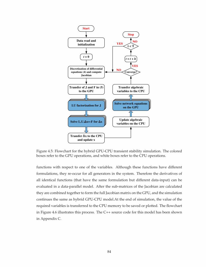
Start
Data read and
initialization
t = 0
Discretization of differential
equations (4) and compute
Jacobian
Transfer of J and F in (5)
to the GPU
LU factorization for J
Solve L.U. x=-F for xUpdate algebraic
variables on the CPU
Solve network equations
on the GPU
Converge?NO
YES
t = t + h
t < TYES
Stop
NO
Transfer algebraic
variables to the CPU
Transfer x to the CPU
and update x
Figure 4.5: Flowchart for the hybrid GPU-CPU transient stability simulation. The coloredboxes refer to the GPU operations, and white boxes refer to the CPU operations.
functions with respect to one of the variables. Although these functions have different
formulations, they re-occur for all generators in the system. Therefore the derivatives of
all identical functions (that have the same formulation but different data-input) can be
evaluated in a data-parallel model. After the sub-matrices of the Jacobian are calculated
they are combined together to form the full Jacobian matrix on the GPU, and the simulation
continues the same as hybrid GPU-CPU model.At the end of simulation, the value of the
required variables is transferred to the CPU memory to be saved or plotted. The flowchart
in Figure 4.6 illustrates this process. The C++ source code for this model has been shown
in Appendix C.
84

Start
Data read and
initialization
t = 0
Discretization of differential
equations (4) and compute
Jacobian
LU factorization for J
Solve L.U. x=-F for xUpdate algebraic
variables on the GPU
Solve network equations
on the GPU
Converge?NO
YES
t = t + h
t < TYES
Stop
NO
Figure 4.6: Flowchart for the GPU-only transient stability simulation. The colored boxesrefer to the GPU operations, and white boxes refer to the CPU operations.
4.6 Experimental Results
In this section we demonstrate results to verify the accuracy and efficiency of the SIMD-
based programming models described in the previous section for the transient stability
simulation of large-scale power systems on the GPU. As mentioned before, the target GPU
in this work is connected to the motherboard of a quad-core CPU. Although the CPU has 4
cores, to precisely control the execution of the CPU and to have a clear comparison, thread
programming was used to force the CPU to run the C++ code on only one of the 4 cores.
Otherwise, the operating system decides each core’s execution at each instant which leads
to a vague evaluation. We selected Windows XP-64 as the host’s operating system. There
were three reasons for choosing this platform: first, we needed a 64-bit operating system,
in order to utilize 8GB of RAM. Second, we expected fewer driver issues on Windows
compared to Linux. Third, within the Windows product line, Windows Vista was not
supported by the NVIDIA GPU Computing platform, leaving Windows XP as the only
choice. For development, we used Microsoft Visual Studio 2005.
85

4.6.1 Simulation Accuracy Evaluation
The accuracy of the programming models was validated using PTI’s PSS/E software pro-
gram. The case study used in this section is the IEEE 39 bus New England test system
whose one-line diagram was shown in Figure 3.15 in Chapter 3. The system data in the
PSS/E format is also given in Appendix E. The complete system can be described by 90
non-linear differential equations and 20 algebraic equations. Several fault locations have
been tested and the results were compared with those of PSS/E. In all cases results from
the proposed programming models match the PSS/E results very well. A sampling of
these results obtained from the hybrid GPU-CPU simulation is presented here. A three-
phase fault happens at Bus 21, at t=1s and it is cleared after 100ms. Gen10 is the reference
generator and the relative machine angles are shown in Figure 4.7 and Figure 4.8. For com-
parison PSS/E results are superimposed in these two figures. As can be seen the transient
stability code is completely stable during the steady-state of the system, i.e. t<1s. During
the transient state and also after the fault is cleared, the program results closely follow the
results from PSS/E. The maximum discrepancy between generator angles from GPU-CPU
co-processing and the PSS/E simulation was found to be 1.46%, based on (4.24):
εδ =max|δPSS/E − δGPU−CPU |
δPSS/E(4.24)
where δPSS/E and δGPU−CPU are the relative machine angles from PSS/E and GPU-
CPU co-processing simulation, respectively.
4.6.2 Computational Efficiency Evaluation
To investigate the efficiency of the proposed SIMD-based programming models for the
transient stability simulation, we show comparative results in this section. Several test
systems of increasing sizes have been used for this evaluation whose specifications are
listed in Table 4.2. The Scale 1 system is the IEEE’s New England test system, illustrated in
Figure 3.15 and verified in the previous section. The Scale 1 system was duplicated several
times to create systems of larger scales. Thus, we obtained test systems of 78, 156, 312, 624,
and 1248 buses. In these systems a flat start was used, i.e. voltage and angle of all buses set
to 1.0∠0◦p.u., and they were modeled in the PSS/E software to find the load flow results.
These results were then fed into the prepared simulation codes.
Three separate simulation codes were prepared: the first code is purely in C++ to be
run sequentially on the CPU (CPU-only), the second is C++ integrated with CUDA to be
86

0 5 10 15-10
0
10
20
30
40
50
60
70
80
90
Time (sec)
Rela
tiv
e m
ach
ine a
ng
les (
deg
rees)
5,10
4,10
3,10
2,10
1,10
GPU-CPU
PSS/E
Figure 4.7: Comparison of relative machine angles collected from hybrid simulator andPSS/E simulation for IEEE 39 bus test system: δi,10 = δi − δ10; i = 1 . . . 5, for a three-phasefault at Bus 21.
0 5 10 15
30
40
50
60
70
80
Time (sec)
Rela
tiv
e m
ach
ine a
ng
les (
deg
rees)
6,10
8,10
9,10
7,10
GPU-CPU
PSS/E
Figure 4.8: Comparison of relative machine angles collected from hybrid simulator andPSS/E simulation for IEEE 39 bus test system: δi,10 = δi − δ10; i = 6 . . . 9, for a three-phasefault at Bus 21.
completely run on the GPU (GPU-only), and the third is also the integration of C++ and
CUDA, however, it uses GPU as the coprocessor (GPU-CPU). The difference between the
second and third programming models was explained in Section III. The execution time of
these three codes was compared for the test systems. In Table 4.2 the columns indicated
by CPU-only, GPU-only, and GPU-CPU list the computation time of each programming
model to simulate a duration of 1580ms with a time-step of 10ms for all systems. The CPU
87
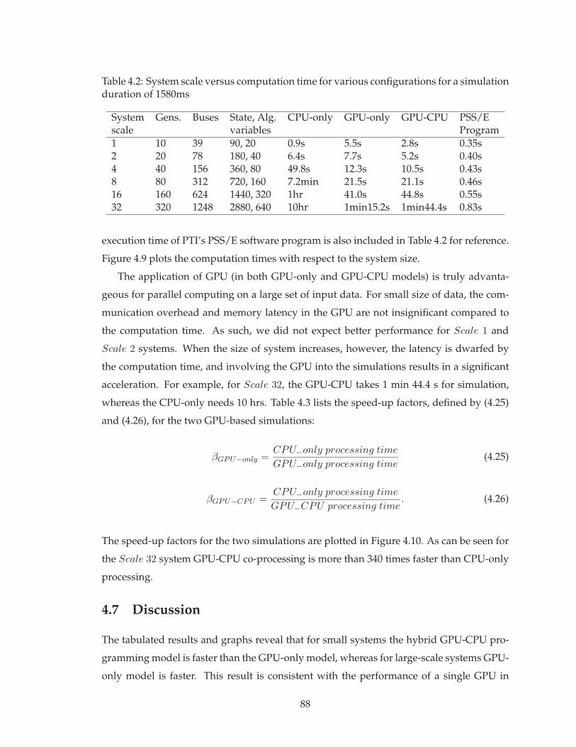
Table 4.2: System scale versus computation time for various configurations for a simulationduration of 1580ms
System Gens. Buses State, Alg. CPU-only GPU-only GPU-CPU PSS/Escale variables Program1 10 39 90, 20 0.9s 5.5s 2.8s 0.35s2 20 78 180, 40 6.4s 7.7s 5.2s 0.40s4 40 156 360, 80 49.8s 12.3s 10.5s 0.43s8 80 312 720, 160 7.2min 21.5s 21.1s 0.46s16 160 624 1440, 320 1hr 41.0s 44.8s 0.55s32 320 1248 2880, 640 10hr 1min15.2s 1min44.4s 0.83s
execution time of PTI’s PSS/E software program is also included in Table 4.2 for reference.
Figure 4.9 plots the computation times with respect to the system size.
The application of GPU (in both GPU-only and GPU-CPU models) is truly advanta-
geous for parallel computing on a large set of input data. For small size of data, the com-
munication overhead and memory latency in the GPU are not insignificant compared to
the computation time. As such, we did not expect better performance for Scale 1 and
Scale 2 systems. When the size of system increases, however, the latency is dwarfed by
the computation time, and involving the GPU into the simulations results in a significant
acceleration. For example, for Scale 32, the GPU-CPU takes 1 min 44.4 s for simulation,
whereas the CPU-only needs 10 hrs. Table 4.3 lists the speed-up factors, defined by (4.25)
and (4.26), for the two GPU-based simulations:
βGPU−only =CPU−only processing time
GPU−only processing time(4.25)
βGPU−CPU =CPU−only processing time
GPU−CPU processing time. (4.26)
The speed-up factors for the two simulations are plotted in Figure 4.10. As can be seen for
the Scale 32 system GPU-CPU co-processing is more than 340 times faster than CPU-only
processing.
4.7 Discussion
The tabulated results and graphs reveal that for small systems the hybrid GPU-CPU pro-
gramming model is faster than the GPU-only model, whereas for large-scale systems GPU-
only model is faster. This result is consistent with the performance of a single GPU in
88

1 2 4 8 16 3210
2
103
104
105
106
107
108
System scale
Com
puta
tion
Tim
e (m
s)CPU−onlyGPU−CPUGPU−only
Figure 4.9: Computation time variation with respect to system scale.
other reported applications. However, there are applications where a GPU may need to
communicate with other entities or use services which may not be accessible to a GPU,
for example in a multiple GPU application. In such cases and with the currently available
GPU technologies, the hybrid GPU-CPU programming model is not only useful but also
unavoidable. Similar to all programmable processors, efficient GPU programming needs
a good understanding of its hardware architecture. Managing the number of required ac-
tive threads for each kernel call, and the number of device-host interactions are essential
to make a timesaving program.
Another useful observation found from the achieved results is the scalability of the pro-
posed hybrid simulator. A system whose performance improves after adding a specific
hardware component, proportionally to the capacity added, is said to be a scalable sys-
tem. In a single GPU expanding the size of data-under-process asks for the co-operation
of more SPs which translates to adding more computing resources. In our experiments the
size of test systems and the hybrid simulators’ elapsed computation time change approxi-
mately at the same rate. In the CPU-only simulation cases, however, the computation time
increases at a rate that is approximately the cube of the system size increment rate.
The last column in Table 4.2 indicates PSS/E’s computation time for the test systems.
It is important to put the lower execution times of PSS/E into proper perspective so as not
to misjudge the performance of the GPU. PSS/E is a mature software program developed
over several decades which incorporates specialized techniques to optimize computational
efficiency for large-scale system simulation. In terms of the numerical methods, the key
89

1 2 4 8 16 320
50
100
150
200
250
300
350
400
450
System scale
Spe
ed−
up
GPU−onlyGPU−CPU
Figure 4.10: Speed-up of GPU-based processing.
Table 4.3: Speed-up comparisonSystem βGPU−only βGPU−CPU
scale1 ×0.16 ×0.32 ×0.83 ×1.24 ×4.05 ×4.78 ×20.1 ×20.516 ×87.8 ×80.332 ×423.5 ×344.8
factors that contribute to PSS/E’s speed are as follows:
1. PSS/E uses the Modified Euler integration algorithm which is an explicit integra-
tion technique (Chapter 26 in [89]). This is a simple and fast method, however, it
can suffer from numerical instability. For a given system configuration, depending
on the time-step value the simulation may either converge or diverge. If it did not
converge, the time-step must be decreased and program must be rerun [90]. In the
proposed GPU-based simulation, the Trapezoidal Rule, an implicit integration algo-
rithm, was used because it is more accurate and avoids numerical instability. How-
ever this method requires an iterative solution of the resulting nonlinear algebraic
equations at each time-step.
2. The outputs of an explicit integrator are not instantaneous functions of their inputs,
and a straightforward non-iterative procedure would be enough to find the deriva-
tives of states, as it happens in PSS/E. However the proposed GPU-based simulator
90

uses the Newton-Raphson method which consumes a large portion of the simulation
time, albeit it gives accurate convergence. At each time-step the Jacobian matrix is
calculated, LU factorized, and then solved using forward-backward substitutions.
3. PSS/E takes advantage of the sparsity of the system matrices. This is an important
factor in its fast and successful management of computer storage. However it should
be noted that presenting PSS/E with a power system network model, whose origi-
nal admittance matrix has a number of nonzero elements that exceed the program’s
allocated capacity, results in an error condition that prevents the use of some, but
not all, of the available iteration algorithms (Chapter 5 in [89]). The purpose in this
chapter was to show how the same implementation of a transient stability algorithm
on a GPU is advantageous with respect to a CPU implementation. Therefore sparsity
was not used in any of the proposed programming models.
4.8 Summary
Transient stability simulation of large-scale power systems is computationally very de-
manding. This chapter investigated the potential of using a GPU to accelerate this sim-
ulation by exploiting its SIMD architecture. Two SIMD-based programming models to
implement the standard method of the transient stability simulation were proposed and
implemented on a single GPU. The simulation codes are quite flexible and extensible; they
are written entirely in C++ integrated with GPU-specific functions. The accuracy of the
proposed methods were validated by the PSS/E software. The efficiency was evaluated
for several large test cases. Based on the results obtained, it can be concluded that:
• Using a GPU for transient stability simulations is highly advantageous when the sys-
tem size is large. As such, for simulating realistic-size power systems the application
of GPU looks promising.
• For small-scale systems the hybrid GPU-CPU simulation was faster than the GPU-
only simulation, while for large-scale systems the GPU-only model was faster.
91

5Multi-GPU Implementation of Large-Scale
Transient Stability Simulation
5.1 Introduction
In Chapter 4 the GPU hardware architecture, based on a NVIDIA GPU, and the SIMD
programming models were explained in detail. The transient stability simulation was im-
plemented on a single GPU, and the results revealed the excellent capabilities of including
GPU as a powerful processor in the power system simulations. However, similar to a
CPU, a GPU also has some computing capacity limitations, that restrict the maximum size
of the problem which can be implemented on it. Simulations of realistic power system of-
ten involve large problem size with onerous calculations. Therefore, this chapter explores
the use of multiple GPUs working in parallel and parallel processing based techniques for
solving large-scale systems.
The chapter1 begins with a review of the multi-GPU simulation application, and con-
tinues by describing the details of the computing system architecture that has been utilized
in this research. Managing multiple GPUs working in parallel to perform a simulation re-
quires specific programming skills which will be highlighted in this chapter. Two parallel
processing based techniques (tearing and relaxation) are implemented on multiple GPUs,
and a comparison between the two methods is presented. The chapter is concluded by
experimental results and discussions.
1Material from this chapter has been submitted: V. Jalili-Marandi, V. Dinavahi, “Multiple GPU implemen-tation for large-scale transient stability simulation,” IEEE Trans. on Power Systems, pp. 1-9, 2010.
92

5.2 Multi-GPU Overview
5.2.1 Applications
The obvious reason for utilizing multiple GPUs for general purpose computing is to achieve
a higher simulation speed, as is the goal in this research. However, compared to the host
main memory, GPU has limited device memory. For applications which require a lot of
storage, device memory limitations can be a major bottleneck for GPU. For this reason,
sometimes running algorithms on multiple GPUs is not only required for faster applica-
tions but also necessary to overcome memory bottlenecks.
There are two possible hardware configurations to use multiple GPUs for the comput-
ing purpose. The first is to mount multiple individual GPUs internally to the motherboard
of the host2 normally using the PCIe buses [92]. The use of multiple GPUs as CUDA de-
vices working on an application is only guaranteed to work if these GPUs are of the same
type [40]. It is important to note that in addition to the GPUs such as GTX 280, described
in Chapter 4, that are applicable to both the graphical tasks as well as general purpose
computing, there are GPU-architecture-based cards which are specifically designed for the
high performance computation with single and double precision floating point (e.g. Tesla
C1060). The Tesla series, introduced by NVIDIA in 2007, is the first GPU generation that
are fully dedicated to general purpose computing.
The second hardware configuration is to use an external computing unit equipped with
multiple GPUs. In this case all the GPUs are compute-specific. For instance the NVIDIA
Tesla S1070 (server version) integrates four Tesla T10 GPUs. This multi-GPU configuration
is used in this research.
5.2.2 Computing System Architecture
The computing system used in this research is one unit of Tesla S1070 manufactured by
NVIDIA [91]. The “Tesla” series of cards are compute-only devices without video output
connectors. The Tesla S1070 is equipped with four independent T10 processors (GPU), and
the programmer decides how many GPUs must be employed in a simulation and the tasks
each GPU must perform. Each of the T10 GPUs is integrated with 4.0GB of memory so that
the total memory of the S1070 unit is 16GB. Delivering a theoretical peak performance of 4
teraflops has made Tesla S1070 an energy efficient teraflop processor. Table 5.1 summarizes
2A comprehensive and practical work is the FASTRA done at the University of Antwerp, Belgium.http://fastra.ua.ac.be
93

Table 5.1: Tesla T10 Processor specifications
Number of SM’s 30Number of SP’s 240Device memory 4GBClock rate 1.3GHzWarp size 32 threadsActive warps/SM 32
the important specifications of a T10 processor. For more hardware architecture informa-
tion of Tesla S1070 the manufacturer data sheets are attached in Appendix D. Each of the
T10 GPUs includes 240 stream processors; thus the Tesla S1070 has a total of 960 stream
processors which can execute thousands of concurrent threads. Therefore, this comput-
ing system that mixes the multi-core CPUs any multiple GPUs provides a heterogenous
computing environment with the optimized performance.
Figure 5.1 illustrates the Tesla S1070 from front and top views. The inside architecture
of Tesla S1070 is shown in Figure 5.2. As depicted in this figure, each pair of the GPUs
are connected to one input/ouput NVIDIA Switch. On the host side, i.e. on the PC moth-
erboard, a Host Interface Card (shown in Figure 5.3) must be plugged into the PCIe bus.
Then by using the NVIDIA PCIe cable connected between the NVIDIA Switch and Host
Interface Card the link between one pair of GPUs of Tesla S1070 and PC host is estab-
lished. To connect the other pair of GPUs, the host computer must have an extra PCIe
slot mounted with another Host Interface Card. Otherwise, to have concurrent access to
4 GPUs two hosts must be used so that each pair of GPUs connects to one host. Figure
5.4 shows the possible configurations to connect a unit of Tesla S1070 to host computers.
The configuration used in this thesis is the same as in Figure 5.4(a) The maximum transfer
bandwidth between the host system and the Tesla processors is 12.8 GB/s.
With all of the highly advanced technology used in Tesla S1070, however, the direct
intercommunication capability of the 4 GPUs (such as using shared memory) is a missed
but promised feature. This means that Tesla S1070 cannot behave as a unified processor.
Therefore, to circulate data among the 4 GPUs of the Tesla S1070, data on one GPU is
first transferred to the host’s main memory (i.e. RAM), and then it is uploaded to the
other GPUs. By using the CPU threads, explained in the next section, this deficiency can
be recovered, but it should be noted that manipulating intensive computation requires
distributing it among existing GPUs.
94

Figure 5.1: Front and top views of Tesla S1070 [91].
5.2.3 Multi-GPU programming
The Tesla S1070 is a CUDA-enabled device. Therefore, all the CUDA programming func-
tionalities explained for the GTX 280 in Chapter 4 are also valid for the Tesla S1070. It was
previously mentioned that the GPU runs its own specified kernel independently but is con-
trolled by the CPU. A single GPU can execute only one kernel at any given time; whereas
a multi-GPU server such as the Tesla S1070 can run multiple kernels (4) simultaneously.
In this chapter we refer to these paradigms serial kernel and parallel kernel executions, re-
spectively Figure 5.5. Thus to have four GPUs working in parallel, in a Tesla S1070 or any
multi-GPU architecture, we require the same number of CPU cores to manage and control
the GPUs simultaneously. This minimizes the overhead that occurs in data copying and
kernel invocation.
Microsoft Visual C++ provides support for creating multi-thread applications with
95

Figure 5.2: Inside architecture of the Tesla S1070 computing system [91].
Figure 5.3: Host Interface Card installing in the host side [91].
Windows XP. There are two ways to program with multiple threads: use the Microsoft
Foundation Class (MFC) library or the C run-time library and the Win32 API [93]. There
also exist some packages and libraries, such as Boost C++ Libraries [94], that can be installed
and utilized for the CPU multi thread programming. In this work, the C-run-time library
was used to have a full control on the synchronization of GPU data-transfer. Writing and
debugging a multi threaded program is inherently a complicated and tricky undertaking,
because the programmer must ensure that objects are not accessed by more than one CPU
thread at a time. Synchronizing the resource access between CPU threads is a common
problem when writing CPU multi threaded applications [93]. Having two or more CPU
threads simultaneously access the same data can lead to undesirable and unpredictable
results. For example, one CPU thread could be updating the contents of a structure while
96

PC Motherboard
with 2 PCIe busesPCIe HIC
PCIe HIC
Tesla S1070 NVIDIA
Switch
NVIDIA
Switch
PC Motherboard
with 1 PCIe bus PCIe HIC
Tesla S1070 NVIDIA
Switch
NVIDIA
Switch
PC Motherboard
with 1 PCIe bus PCIe HIC
(a)
(b)
Figure 5.4: Possible configurations of connecting Tesla S1070 to host CPU system: (a) usingone host, (b) using two hosts.
another CPU thread is reading the contents of the same structure. It is unknown what data
the reading thread will receive: the old data, the newly written data, or possibly a mixture
of both. To control synchronization among the CPU threads, events are used. Events allow
CPU threads to be synchronized by forcing them to pause until a specific event be set or
reset.
Figure 5.6 illustrates how the application of multi thread programming is managed to
operate up to 4 GPUs connected to a quad-core CPU. The main thread on the CPU first
creates four child threads which are responsible for handling one GPU each. Creating
the CPU threads is a time-consuming operation; thus once they are created they should
be used for the whole of the simulation time duration. The main thread also creates two
event arrays called Start and End. Each element of these arrays is used as a notification
signal between the main thread and one of the child threads to determine the initiation or
97

kernel 1
kernel 2
kernel N
time
t=0
t=T
Tesla S1070
GTX 280
kernel 1
kernel 2
kernel N
Tesla T10
kernel 1
kernel 2
kernel N
Tesla T10
kernel 1
kernel 2
kernel N
Tesla T10
kernel 1
kernel 2
kernel N
Tesla T10
(a) (b)
Figure 5.5: (a) Serial kernel execution on a single GPU, (b) Parallel kernel execution on amulti-GPU system.
termination of a specific action. Child threads begin execution by setting one individual
device (GPU) and initializing it, and then wait until the Start event is set. As soon as
the main thread sets the Start event the computations in the individual GPU belonging
to each child thread are activated. The main thread goes into a waiting state until all the
threads are done by the GPU computations and the End event is set. Thereafter, four child
threads will exchange and update the required data with the help of the CPU, and the
simulation continues. At each child thread when the GPU computation is done, in addition
to setting the End event, it is also required to reset the Start event to prevent running of
the child threads until the data update is done by the main thread and the Start command
is released. Therefore, by appropriate use of the Start and End events the synchronization
between child threads and consequently the multiple GPUs is orchestrated.
5.3 Implementation of Parallel Transient Stability Methods onTesla S1070
In Chapter 2 two categories of the parallel processing based techniques, i.e. tearing and re-
laxation methods, were explained. In this section one method belonging to each category
is selected to be implemented on the parallel architecture of Tesla S1070. From the cate-
98

NO
(wait)
main( )
create threads
and events
set Start events
are all End
events set?
Yes
data exchange
reset all events
NO
(wait)
update events status
update events status
CPU thread #1
CPU thread #4
set device, and
initialize GPU#1
is Start event set?
computations on
GPU#1
reset Start event;
set End event
Yes
set device, and
initialize GPU#4
is Start event set?
computations on
GPU#4
reset Startevent;
set End event
Yes
NO
(wait)
Figure 5.6: The programming application for general purpose multi-GPU computationusing a quad-core CPU.
gory of tearing methods, the Block Incomplete LU decomposition method, and from the
relaxation group the Instantaneous Relaxation method, described in Chapter 3, are being
examined.
5.3.1 Tearing Methods on Multi GPU
In the GPU-only programming model described in Chapter 4, three major parts can be
discerned: (1) integration of differential equations and Jacobian matrix computation, (2)
LU decomposition of the Jacobian matrix, and (3) solution of the linear algebraic equations,
updating and saving the required variables, and GPU-CPU communication time. To get
an estimate of the timing load of each part, the results of the elapsed time for these specific
parts as a fraction of the total simulation time, and for various system sizes used in Chapter
4 are listed in Table 5.2. These results reveal that LU decomposition (i.e. PART2 in Table
5.2) is the most time-consuming part of the simulation. Thus, the part that would benefit
most from using multiple GPUs to reduce the simulation time is the LU factorization. In
this section we will use parallel processing to significantly improve this timing.
Tearing methods take advantage of the block structure of the system of equations. In a
99

Table 5.2: System scale versus fraction of simulation time elapsed for each major part.PART1: integration and Jacobian matrix computations, PART2: LU decomposition, andPART3: linear algebraic solution, updating and saving variables, and communication time.
System scale PART1 PART2 PART31 23% 55% 22%2 14% 70% 16%4 8% 81% 12%8 4% 88% 8%16 2% 91% 7%32 1% 92% 7%
system of equations where the dependency matrix is sparse, tearing can be used to achieve
decomposition while maintaining the numerical properties of the method used to solve
the system [62]. The Jacobian matrix resulting from the linearization step of the transient
stability simulation is a case that fits this condition well. The Jacobian matrix of a large-
scale power system for transient stability study has a sparse diagonally-blocked structure.
The Incomplete LU factorization (ILU) is widely recognized as effective method for a
preconditioned iterative sparse linear system solution. A preconditioner is any form of
implicit or explicit modification of an original linear system that makes it easier to solve
by an iterative method. For example, scaling all rows of a linear system to make the diag-
onal elements equal to one is an explicit form of preconditioning. The ILU method entails
a decomposition of the form A = LU −R, where L and U have the same nonzero structure
as the lower and upper parts of A, and R is the residual or error of the factorization [95].
This incomplete factorization, known as ILU(0), is easy and inexpensive to compute, but it
often leads to a rough approximation and imposes more iterations to the applied iterative
scheme. Generally, more accurate ILU factorizations require fewer iterations to converge.
Thus, several alternatives of this approach have been developed by allowing more fill-ins
in the L and U matrices. One alternative that is useful for sparse matrices is to perform
the LU-decomposition only at locations where A originally has non-zeros. A variant of
this approach is the Block ILU in which the decomposition is conducted only along the
main diagonal [95]. Figure 5.7 shows the original sparse matrix divided into diagonal
sub-matrices which locally are decomposed using ILU. Because these blocks do not com-
municate with each others and can be individually decomposed, this scheme fits well in a
parallel processing based architecture.
Considering the multi-GPU programming concepts explained in the previous section
100

U2
L2
Jn
J1
J2
Figure 5.7: Sparse diagonally blocked matrix is a suitable case for the ILU method.
(such as creating and managing CPU threads and events), Figure 5.8 illustrates the distri-
bution of computations among the GPUs of a Tesla S1070 unit. As shown in the pseudo
code, the discretization of the DAEs and computation of the Jacobian matrix for the whole
system are done on the main thread on the CPU. The Jacobian matrix is then decomposed
into n sub-matrices which are then transferred to each of the GPUs. GPUs concurrently de-
compose the sub-matrices into their L and U factors. Due to the parallel operation of GPUs,
their computation loads must be equal to have an efficient simulation. Thus, the sub-
matrices must have equal or approximately equal size. Moreover, the size of sub-matrices
is an important factor: if they are too small the overall efficiency of using GPUs will be
lost. After all GPUs are done with the factorization steps, the L-U factors are transferred
to the CPU main memory, and then uploaded to one of the GPUs to build the original-size
LU factor and perform the remaining calculations.
5.3.2 Relaxation Methods on Multiple GPUs
In Chapter 3 the Instantaneous Relaxation (IR) method was proposed and implemented
on the PC-cluster based simulator made up of multiple CPUs. The important advantage
of this method in the transient stability study of large-scale power systems is its ability to
make a coarse-grain decomposition which allows breaking down the large DAE systems
into smaller pieces and distributing the individual computations to specified processors.
These processors need to communicate only once at each time-step.
101

do ILU for the selected
blocks on GPU#4
update events status
update events status
NO
(wait)
NO
(wait)
set device, and initialize
GPU#4
is Start
event set?
reset Start event;
set End event
Yes
CPU thread#4
do ILU for the selected
blocks on GPU#1
set device, and initialize
GPU#1
is Start
event set?
reset Start event;
set End event
Yes
CPU thread #1main()
{
3.distribute J among CPU threads;
}
end of while
print and save output results;
4.wait for the event update;
5.gather small L’s and U’s from GPUs;
6.transfer L’s and U’s to one GPU,
and construct the complete L and U;
7.solve the linear system;
8.check the convergence condition;
9.update variables;
go for the next time step;
read system input data;
create CPU threads and events;
while time < Sim_time
2.compute Jacobian matrix (J);
1.discretize differential equations;
Figure 5.8: ILU-based tearing method implementation on multiple GPUs.
In this section the IR method will be implemented on the multi-GPU architecture of
Tesla S1070. This provides a high degree of parallelization for the transient stability study.
First, the solution algorithm is inherently parallel, and second, this algorithm is imple-
mented on up to 4 GPUs each with a massively data-parallel architecture. In other words,
implementing of the IR method on a multiple GPUs is actually the intersection of algorithm-
level-parallelism and data-parallelism.
Figure 5.9 illustrates how the Instantaneous Relaxation method is implemented on the
4 GPUs of a Tesla S1070 system. Comparing this figure with Figure 5.8 it can be seen that
in the IR method the system decomposition and consequently the parallelization happen
at the top level of computations, while in the tearing based approach parallelization is in
the inner loop of the procedure. Thus, in case the convergence condition in the ILU-based
tearing method is not fulfilled, the loop must be repeated which multiplies the commu-
nication time between the Tesla S1070 and CPU memory. Whereas, from the GPU pro-
gramming perspective efficient programs are ones which require the minimum amount of
GPU-CPU communication. To practically confirm this statement, Table 5.3 lists the exper-
imental results showing the maximum bandwidth rate of the Tesla T10 processors inside
the Tesla S1070 system. In this Table “Device” refers to a single Tesla T10 processor, and
102

Table 5.3: Tesla T10 processor bandwidth test results
Host-to-Device 1.35GB/sDevice-to-Host 1.62GB/sDevice-to-Device 73.1GB/s
“Device-to-Device” means the operations inside one GPU, i.e. not the interconnection be-
tween 2 GPUs. As it can be seen, the Host-Device bandwidth for both directions is lower
than that of the device to device rate. Therefore, especially in the application of multiple
GPUs where data transfer is unavoidable, the GPU-CPU communication must be reduced
to minimize simulation time. This is what the IR method provides perfectly. In the next
section, a comprehensive efficiency comparison between the tearing and relaxation types
parallelization will be shown and discussed.
In addition to the high parallelization offered by the IR method, its implementation
on both single GPU (serial kernel) as well as multiple GPUs (parallel kernel) covers the
maximum size limitation imposed by CUDA/CUBLAS application. In the current version
of CUBLAS API, BLAS2 functions are specified for the single or double precision matrix-
vector operations. For example, cublasStrsv() solves a system of equations of the form:
op(A) ∗ x = b,
where op(A) = A or op(A) = AT ,
b and x are n-element single-precision vectors, and A is an n × n, upper or lower tri-
angular matrix consisting of single-precision elements. This function plays an important
role in the solution of a system of linear algebraic equations that have already been LU fac-
torized. cublasStrsv() takes n as an input argument that determines the number of rows
and columns of the matrix A. In the current implementation of CUBLAS, n must not ex-
ceed 4070 for the single-precision entries. For the double-precision function n is limited
to 2040 [87]. This is an unexplained boundary, imposed by the GPU manufacturer, that
does not allow the programmer to go beyond systems that may include matrices with the
dimension larger than these limits. For instance, the size of Jacobian matrix in the tran-
sient stability stability simulation of a power network within m machines each of which
is modeled by 9 state variables is 9m × 9m. Thus, the largest system that can be modeled
in a single GPU with the traditional approach cannot include more than 450 machines.
In the IR method, however, the system is decomposed into subsystems which are solved
individually. Consequently, regardless of its serial or parallel implementation of the IR
method, each subsystem can use the maximum compute capacity of the available hard-
103

do transient stability steps
on GPU#4
update events status
NO
(wait)
set device, and initialize
GPU#4
is Start
event set?
reset Start event;
set End event
Yes
CPU thread#4
main()
{
1.decompose system into subsystems;
}
end of while
print and save output results;
c)wait for the event update;
b)conduct the transient stability
computations on each GPU and for
each subsystem;
go for the next time step;
read system input data;
2.create CPU threads and events;
while time < Sim_time
d)gather and exchange data;
3.distribute subsystems among GPUs;
a)set the Start event;
do transient stability steps
on GPU#1
update events status
NO
(wait)
set device, and initialize
GPU#1
is Start
event set?
reset Start event;
set End event
Yes
CPU thread #1
Figure 5.9: IR method implementation on multiple GPUs.
ware. This is the direct result of decomposing the system of DAE from the differential
equations level and before performing the discretization step (i.e. top level). In the ILU-
based tearing method described in the previous section, although the Jacobian matrix is
torn into smaller sub-matrices, eventually they must be rebuild the original-size LU ma-
trix to be used in cublasStrsv() function.
5.4 Experimental Results
5.4.1 Work-station and Test Systems
In this section we demonstrate results to verify and compare the efficiency of the parallel
processing based techniques described in the previous section. As mentioned before, the
target computing system is a unit of Tesla S1070 that is connected to the motherboard of
a quad-core CPU supported by 8GB of memory (RAM). Depending on the size of com-
putations being done on the multi-GPU system, using the same amount of CPU memory
(RAM) as the GPUs have is recommended to achieve better performance. For example, in
the case of running 4 GPUs of the Tesla S1070, the CPU should be supported by 16GB of
RAM; however, in our case the host motherboard can support a maximum of 8GB of RAM.
Thus, the simulation time results that are shown in this section can be improved simply by
104

Table 5.4: Test System Scales
System scale Generators Buses1 10 392 20 784 40 1568 80 31216 160 62432 320 124864 640 2496128 1280 4992180 1800 7020
upgrading the host-side memory.
The accuracy of the simulation models has been investigated and discussed for the
single GPU case in Chapter 4. In this chapter also, we use the IEEE’s New England test
system and develop its multiplicands by using PTI’s PSS/E software. The steady-state
and dynamic stability of these systems have been examined and verified. Although these
are fictitious systems, the important advantage of using them as test cases is that they let
us to explore the performance of the GPU-based simulation statistically and gradually. In
addition to the systems used in Chapter 4, in this chapter systems with Scales 64, 128,
and 180 have been developed. The single-line diagrams for these systems are given in the
Appendix E, and Table 5.4 summarizes the specifications of these cases. The Scale 180 is
constructed based on the discussion provided in the previous section that the maximum
computing capacity of each GPU for the prepared model is 450 generators. This system
is built so that all GPUs of the Tesla S1070 become fully populated (4 × 450 = 1800 gen-
erators). The admittance matrix and load flow results of PSS/E simulating these systems
were saved in a text format file to be fed into the prepared programs for the tearing and IR
methods.
5.4.2 Transparency
Both parallel processing based methods are implemented to work with 1 to 4 GPUs, de-
pending on the required computing capacity. This issue in the parallel processing software
development is referred as transparency, which means the ease with which software written
for a set number of processors can be reformulated for another number of processors [49].
Although the SIMD hardware architecture of GPU and the way kernels are invoked and
run by many threads offer a high degree of transparency, the developed software is ef-
105

1.4 2.2 4 8 17
42.5
131.4
460.5
1.4 2.8 6.1 14.9
40.5
0
50
100
150
200
250
300
350
400
450
500
2 4 8 16 32 64 128 180
System scale
Co
mp
uta
tion
tim
e (
s)
IR ILU
No
t A
pp
licab
le
No
t A
pp
licab
le
No
t A
pp
licab
le
1.3 1.9 3.67.1
14.5
32.9
86.2
1.1 2.1 4.18.8
20.4
53.7
0
10
20
30
40
50
60
70
80
90
100
1 2 4 8 16 32 64
System scale
Com
pu
tati
on
tim
e (
s)
IR ILU
Not
Ap
pli
cable
(a)
(b)
Figure 5.10: Multi-GPU simulation: (a) 2 GPUs, (b) 4 GPUs.
fectively controllable by changing one variable at the compile time to work with various
numbers of parallel GPUs. In this section the 2 and 4 GPUs implementation will be shown.
Graphs shown in Figure 5.10 compare the computation time of the IR and ILU-based
tearing methods. In Figure 5.10.a the results for utilizing 2 GPUs illustrates that as the
system enlarges the IR method accelerates more than ILU method, so that for the largest
106
applicable system, i.e. Scale 32, the IR is 1.6 times faster than ILU method. Moreover,
Scale 64 and higher are not implementable with the ILU method, due to GPU hardware
restriction, while the IR overcomes the limitation and can simulate larger system. These
systems that are not implementable are shown as “Not Applicable” in graphs. The largest
system that can be implemented by exploiting 2 parallel GPUs is Scale 90, which includes
900 fully detailed generator models, not shown in this figure.
Figure 5.10.b shows the computation time for the case of using 4 parallel GPUs. In
this case the Scale 1 is ignored, because the communication and computation times are
too similar to reveal any computing advantage of including multiple GPUs. From the
achieved results it is clear that IR implementation is faster than ILU-based simulation, so
that for the largest applicable system for both methods, i.e. Scale 32, the IR is 2.4 times
faster than ILU method. Furthermore, very large-scale systems as Scales 64, 128, and 180
have been simulated by the IR method. Scale 180 is the system that entirely occupies Tesla
S1070 to solve 19800 DAEs.
5.4.3 Scalability
The other important observation is the scalability characteristic of the IR method. The
Scaling Factor (SF) is defined as:
SF =computation time of Single GPU
computation time of Multiple GPUs(5.1)
The SF reveals how much the parallel multi-GPU simulation is efficient compared with
the single-GPU simulation. Ideally, and for an available hardware, we expect that in case
of using n parallel processors simultaneously running to solve a problem which takes T
seconds on a single processor, the simulation time would break down to Tn seconds. How-
ever, this is not true in practice due to several software development issues such as task
scheduling, processors’ communication, and the parallel processing algorithm. Thus, SF
is always less than n, and the closer it is to n, the higher is the efficiency of multi processing
based technique. This factor is computed for the IR as well as ILU-based methods, for 2
and 4 GPUs, and for the system scales that are applicable to both methods. The results are
depicted in Figs. 5.11 and 5.12. For the IR method in both the 2 and 4 GPUs, as the test sys-
tem expands, the SF factor grows closer to the number of parallel GPUs in use. This means
that the IR method is scalable, and if somehow the communication time is reduced, for ex-
ample by upgrading the hardware or advancement in GPU cluster technology, the SF will
107
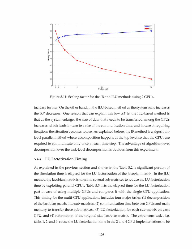
1 2 4 8 16 321
1.1
1.2
1.3
1.4
1.5
1.6
1.7
1.8
1.9
System scale
Scal
ing
Fac
tor
IRILU
Figure 5.11: Scaling factor for the IR and ILU methods using 2 GPUs.
increase further. On the other hand, in the ILU-based method as the system scale increases
the SF decreases. One reason that can explain this low SF in the ILU-based method is
that as the system enlarges the size of data that needs to be transferred among the GPUs
increases which leads in-turn to a rise of the communication time, and in case of requiring
iterations the situation becomes worse. As explained before, the IR method is a algorithm-
level parallel method where decomposition happens at the top level so that the GPUs are
required to communicate only once at each time-step. The advantage of algorithm-level
decomposition over the task-level decomposition is obvious from this experiment.
5.4.4 LU Factorization Timing
As explained in the previous section and shown in the Table 5.2, a significant portion of
the simulation time is elapsed for the LU factorization of the Jacobian matrix. In the ILU
method the Jacobian matrix is torn into several sub-matrices to reduce the LU factorization
time by exploiting parallel GPUs. Table 5.5 lists the elapsed time for the LU factorization
part in case of using multiple GPUs and compares it with the single GPU application.
This timing for the multi-GPU applications includes four major tasks: (1) decomposition
of the Jacobian matrix into sub-matrices, (2) communication time between GPUs and main
memory to transfer these sub-matrices, (3) LU factorization for each sub-matrix on each
GPU, and (4) reformation of the original size Jacobian matrix. The extraneous tasks, i.e.
tasks 1, 2, and 4, cause the LU factorization time in the 2 and 4 GPU implementations to be
108

2 4 8 16 32
1.4
1.6
1.8
2
2.2
2.4
2.6
2.8
3
3.2
3.4
System scale
Scal
ing
Fac
tor
IRILU
Figure 5.12: Scaling factor for the IR and ILU methods using 4 GPUs.
Table 5.5: System size versus LU decomposition elapsed time (in seconds) for single, 2,and 4 GPUs applications.
System scale 1 GPU 2 GPUs 4 GPUs1 1.1 0.7 Not Applied2 2.4 1.6 0.94 5.1 3.3 2.28 10.8 7.8 5.216 23.3 17.5 12.332 54.6 44.5 33.1
more than half or quarter of that in the single GPU application.
5.5 Summary
The main goal in this chapter was to demonstrate the practical aspects of utilizing multi-
ple GPUs. A parallel processing technique can be implemented on any parallel processor
based hardware, for example using a cluster consisting of hundreds of PC’s. However,
employing a large cluster has some drawbacks as well: it is quite expensive, is not always
available, takes a lot of space and requires considerable maintenance. By including GPU
units in the simulation and appropriate programming of GPUs, a regular PC can have the
performance of a super computer with much less price and energy usage. Moreover, these
GPUs are affordable for personal, research, and industry applications.
109

In this chapter, two parallel processing based techniques implemented on a Tesla S1070
unit. The techniques used here are from tearing and relaxation categories, explained in
Chapters 2 and 3. The experimental results revealed that algorithm-level decomposition,
as it happens in the Instantaneous Relaxation method, is more efficient than task level
decomposition.
Although the multi-GPU server with its current technology looks very capable, its API
still is in its infancy. Performance of the multi-GPU algorithm can be further increased by
direct GPU to GPU communication. We await NVIDIA’s CUDA support for direct inter-
GPU communication instead of communication through the CPU.
110

6Summary and Conclusions
Transient stability analysis is a major requirement for the planning and safe operation of
power systems. It is the core of any DSA tool in the energy management system. However,
time domain transient stability simulation of large-scale power systems is computationally
very demanding. The transient stability problem is rich in parallelism which makes it very
suitable for applying parallel processing based techniques.
The goal in this thesis is to accelerate the transient stability simulation. To do so, the in-
vestigation in this thesis branched into two directions. In part one the focus is the real-time
implementation of transient stability simulation. As the real-time simulator has a parallel
processor architecture, it is unavoidable to have a parallel processing based technique to
use the simulator’s capacity. The IR method was proposed and successfully implemented
for this purpose, and is shown to give both accuracy and efficiency for PC-cluster based ar-
chitecture. The main outcome of this approach is that it uses the program-level parallelism
that inherently exists in the nature of the transient stability problem. In the second part the
objective is still the acceleration of the transient stability simulation for larger systems but
by using the general purpose computing capacity of the GPUs. The use of GPU requires
the rethinking and re-engineering of the problem solution in a SIMD-based programming
model. The results obtained in this part revealed the advantage of GPU-based simulation
over the CPU-based one for large-scale systems. By using single GPU it became possible
to model large-scale systems that take several hours of CPU time in a few minutes. Inte-
grating the IR method with the multiple GPUs was the other achievement of this thesis
111

that not only increased the scale of largest implementable system but also overcame the
limitation existed in the current GPUs.
6.1 Contributions of This Thesis
The main contributions of this thesis are summarized as follows:
• This thesis has a significant practical value. Although transient stability has been
formulated and it has a rich literature resources, in this thesis the effort was to aggre-
gate the abstract of all the required equations, for synchronous machine and network
modeling, and step-by-step numerical methods to solve these equations. Moreover,
in both real-time implementation as well as single/multiple GPU programming the
achieved experiences and difficulties that may exist were clearly explained. This type
of knowledge cannot be usually found in power systems literature.
• The IR method proposed in Chapter 3 showed an efficient performance for both real-
time simulation as well as multiple GPU implementation. Integrating this method
with the slow coherency based partitioning and its implementation on a general pur-
pose state-of-the-art real-time simulator resulted in an inexpensive and efficient real-
time simulator. In the GPU applications, the IR method was also very helpful to
overcome the technology restriction existing in the present GPUs. By the use of this
method it was possible to conduct the transient stability simulation of large-scale
power systems which are modeled in detail.
• The software developed for both real-time simulation as well as GPU application,
is designed in such a way to be easy to expand to include more models of power
system elements in its library. It is also easy in both cases to change the number of
processor nodes or GPUs which are running in parallel.
• This is the first time that GPU is used for dynamic computations in power systems.
This research will introduce GPUs to the power systems experts and inspire them to
use GPUs for other burdensome computations such as load flow and electromagnetic
transient studies.
6.2 Directions for Future Work
This research can be continued in several ways for the transient stability simulation of
power systems. First, the software developed for both real-time simulation as well as GPU
112

codes have the capacity to be further improved. For instance, including more models for
synchronous machines, AVR, PSS, and loads, adding more elements such as protection
devices, as well as the ability for performing various types of contingency studies all are
cases that lead to provide a complete set of transient stability tool. Having this tool and
using the IR algorithm as the core of parallel processing method the general purpose real-
time simulator can be utilized as a real-time transient stability simulator.
It is anticipated that the GPU can play an important role in realizing the ultimate goal of
online or real-time dynamic security assessment in the energy control center. The transient
stability simulation algorithm in this research work employed the implicit Trapezoidal
integration method along with the iterative Newton-Raphson procedure. However, as
reported in Chapter 1, there exist many other possibilities for solving the nonlinear DAEs
applicable to the transient stability problem, such as:
• explicit or implicit integration methods
• iterative and non-iterative solvers
• simultaneous or partitioned solution approaches
• application of sparse methods to solve linear algebraic equations [96].
In addition, it is also possible to implement other parallel processing based techniques to
investigate higher speed-ups. It is predicted that if a method accelerates the CPU-based
simulation, it would also accelerate the GPU-based model, if that approach was efficiently
implemented on the GPU.
Existing real-time simulators used in the power system area are clusters made up of
CPU or DSP based hardware. Each rack of these simulators costs several hundreds of
dollars and are not affordable for all industry and academic customers. Moreover, the
maximum size of the system that can be simulated by a rack of PC-cluster is very limited.
The price of the GPU-cluster is much lower than the PC-cluster simulator while its com-
puting capacity is much higher. Therefore, a worthwhile research goal is to move toward
using GPUs for the real-time simulations. Certainly, GPU has the capacity for this purpose,
but the important points are how to manage or force a GPU code to run in real-time and
second, how to perform the hardware-in-the-loop simulations. The former is mainly the
matter of software development while the later is the hardware issue.
Recently, NVIDIA represented next-generation of CUDA architecture GPUs named
Fermi. The complexity of the Fermi architecture is managed by a multi-level program-
113

ming model that allows software developers to focus on algorithm design rather than the
details of how to map the algorithm to the hardware, thus improving productivity. The
most important difference of this new generation of GPUs in comparison with existing
ones is that Fermi supports simultaneous execution of multiple kernels from the same ap-
plication, each kernel being distributed to one or more SMs on the device. This capability
avoids the situation where a kernel is only able to use part of the device and the rest goes
unused [97]. Exploiting this technology would let us implement a program or task level
parallel transient stability simulation algorithm (such as Instantaneous Relaxation or ILU
methods) on a single Fermi GPU in the future.
114

Bibliography
[1] R. Schainker, G. Zhang, P. Hirsch, C. Jing, “On-line dynamic stability analysis usingdistributed computing,” Power and Energy Society General Meeting, Conversion and Deliv-ery of Electrical Energy in the 21st Century, pp. 1-7, 2008.
[2] EPRI TR-104352, “Analytical Methods for Contingency Selection and Ranking for Dy-namic Security Analysis,” Power and Energy Society General Meeting, Conversion and De-livery of Electrical Energy in the 21st Century, Project 3103-03 Final Report, Sept. 1994.
[3] IEEE Std 100, “The Authoritative Dictionary of IEEE Standards Terms Seventh Edi-tion,” 2000.
[4] H. W. Dommel, “Techniques for analyzing electromagnetic transients,” IEEE Comput.Appl. Power, vol. 10, Issue 3, pp. 18-21, July 1997.
[5] IEEE/CIGRE Joint Task Force on Stability Terms and Definitions, “Definition and clas-sification of power system stability,” IEEE Trans. Power Syst., vol. 19, no. 2, pp. 1387-1401,May 2004.
[6] E. W. Kimbark, Power system stability, vol. 1, New York: J. Wiley, 1948.
[7] M. Pavella, P. G. Murthy, Transient stability of power systems: theory and practice, Chich-ester, New York: Wiley, 1994.
[8] P. M. Anderson, A. A. Fouad, Power system control and stability, Iowa State UniversityPress, 1977.
[9] P. Kundur, Power system stability and control, McGraw-Hill, 1994.
[10] IEEE Std 1110-2002, “IEEE guide for synchronous generator modeling practices andapplications in power system stability analyses,” IEEE Power Eng. Soc., pp. 1-81, Nov.2003.
[11] A. A. Fouad, V. Vittal, Power system transient stability analysis using the transient energyfunction method, Englewood Cliffs, N.J.: Prentice Hall, 1992.
[12] B. Stott, “Power system dynamic response calculations,” Proc. of IEEE, vol. 67, no. 2,pp. 219-241, Jul. 1979.
115

[13] P. M. Anderson, B. L. Agrawal, J. E. Van Ness, Subsynchronous resonance in powersystems, IEEE PRESS, New York, 1990.
[14] M. Sultan, J. Reeve, R. Adapa, “Combined transient and dynamic analysis of HVDCand FACTS systems,” IEEE Trans. Power Del., vol. 13, no. 4, pp. 1271-1277, Oct. 1998.
[15] T. Berry, A. R. Daniels, R. W. Dunn, “Real-time simulation of power system transientbehaviour,” Proceedings of 3rd International Conference on Power System Monitoring andControl, pp. 122-127, June 1991.
[16] D. Jakominich, R. Krebs, D. Retzmann, A. Kumar, “Real time digital power systemsimulator design considerations and relay performance evaluation,” IEEE Trans. PowerDelivery, vol. 14, no. 3, pp. 773-781, July 1999.
[17] M. O. Faruque, V. Dinavahi, “Hardware-in-the-loop simulation of power electronicsystems using adaptive discretization,” IEEE Trans. Industrial Electronics, vol. 57, no. 4,pp. 1146-1158, Apr. 2010.
[18] R. H. Park, E. H. Bancker, “System stability as a design problem,” AIEE Trans., vol.48, pp. 170-194, 1929.
[19] O. G. C. Dahl, Electric power circuits, Vol. II: Power system stability, McGraw-Hill, NewYork, 1938.
[20] H. H. Skilling, M. H. Yamakawa, “A graphical solution of transient stability,” ElectricalEng., vol. 59, pp. 462-465, 1940.
[21] M. Pavella, D. Ernst, D. Ruiz-Vega, Transient stability of power systems: a unified approachto assessment and control, Kluwer Academic Publishers, 2000.
[22] P. L. Dandeno, P. Kundur, “A non-iterative transient stability program including theeffects of variable load-voltage characteristics,” IEEE Trans. Power App. Syst., vol. PAS-92, pp. 1478-1484, 1973.
[23] N. Stanton, S. N. Talukdar, “New integration algorithms for transient stability stud-ies,” IEEE Trans. Power App. Syst., vol. PAS-89, pp. 985-991, May 1970.
[24] M. M. Adibi, P. M. Hirsch, J. A. Jordan, “Solution methods for transient and dynamicstability,” Proc. IEEE, vol. 62, pp. 951-958, July 1974.
[25] H. L. Fuller, P. M. Hirsch, M. B. Lambie, “Variable integration step transient analysis-VISTA,” Proc. IEEE PICA Conf., pp. 156-161, 1973.
[26] W. D. Humpage, K. P. Wang, Y. W. Lee, “Numerical integration algorithms in power-system dynamic analysis,” Proc. Inst. Elec. Eng., vol. 121, pp. 467-473, 1974.
116

[27] G. Kron, “Diakoptics-piecewise solutions of large systems,” Elect. J., London, vol. 158-vol. 162, also published by McDonald, London, 1963.
[28] M. La Scala, M. Brucoli, F. Torelli, M. Trovato, “A gauss-jacobi-block-newton methodfor parallel transient stability analysis,” IEEE Trans. Power Syst., vol. 5, no. 4, pp. 1168-1177, May 1990.
[29] M. L. Crow, M. Ilic, “The parallel implementation of the waveform relaxation methodfor transient stability simulations,” IEEE Trans. Power Syst., vol. 5, no. 3, pp. 922-932,Aug. 1990.
[30] M. La Scala, R. Sbrizzai, F. Torelli, “A pipelined-in-time parallel algorithm for tran-sient stability analysis,” IEEE Trans. Power Syst., vol. 6, no. 2, pp. 715-722, May 1991.
[31] F. L. Alvarado, “Parallel solution of transient problems by trapezoidal integration,”IEEE Trans. Power Appar. and Syst., vol. PAS-98, no. 3, pp. 1080-1090, May/June 1979.
[32] M. Shahidehpour, Y. Wang, Communication and Control in Electric Power Systems: Ap-plications of Parallel and Distributed Processing. New Jersey, US: John Wiley and Sons,2003.
[33] M. J. Flynn, “Very high speed computing systems,” Proc. of the IEEE, pp. 1901-1909,Dec. 1966.
[34] H.H. Happ, C. Pottle, K.A. Wirgau, “An assessment of computer technology for largescale power system simulation,” Power Industry Computer Applications Conference, pp.316-324, May 1979.
[35] F. M. Brasch, J. E. Van Ness, S. C. Kang, “Simulation of a multiprocessor network forpower system problems,” IEEE Trans. Power App. Syst., vol. PAS-101, no. 2, pp. 295-301,Feb. 1982.
[36] S. Y. Lee, H. D. Chiang, K. G. Lee, B. Y. Ku, “Parallel power system transient stabilityanalysis on hypercube multiprocessors,” IEEE Trans. Power Syst., vol. 6, no. 3, pp. 1337-1343, Aug. 1991.
[37] H. Taoka, S. Abe, S. Takeda, “Fast transient stability solution using an array proces-sor,” IEEE Trans. Power App. Syst., vol. PAS-102, no. 12, pp. 3835-3841, Dec. 1983.
[38] M. Takatoo, S. Abe, T. Bando, K. Hirasawa, M. Goto, T. Kato, T. Kanke, “Floatingvector processor for power system simulation,” IEEE Trans. Power App. Syst., vol. PAS-104, no. 12, pp. 3361-3366, Dec. 1985.
[39] P. Forsyth, R. Kuffel, R. Wierckx, J. Choo, Y. Yoon, T. Kim, “Comparison of transientstability analysis and large-scale real time digital simulation,” Proc. of the IEEE PowerTech., vol. 4, pp. 1-7, Sept. 2001.
117

[40] NVIDIA, “NVIDIA CUDA Programming Guide,” June, 2008.
[41] S. C. Savulescu, Real-time stability assessment in modern power system control centers,IEEE Press Series on Power Engineering, 2009.
[42] R. Krebs, E. Lerch, O. Ruhle, “Blackout prevention by dynamic security assessmentafter severe fault situations,” CIGRE Proc. on Relay Protection and Substation Automationof Modern Power Systems, pp. 1-9, Sept. 2007.
[43] J. I. Mitsche, “Stretching the limits of power system analysis,” IEEE Computer Appli-cations in Power, pp. 16-21, Jan. 1993.
[44] G. Aloisio, M. A. Bochicchio, M. La Scala, R. Sbrizzai, “A distributed computingapproach for real-time transient stability analysis,” IEEE Trans. Power Syst., vol. 12, no.2, pp. 981-987, May 1997.
[45] F. F. de Mello, J. W. Felts, T. F. Laskowski, L. J. Opple, “Simulating fast and slowdynamic effects in power systems,” IEEE Computer Applications in Power Syst., pp. 33-38, July 1992.
[46] Y. Chen, C. Shen, J. Wang, “Distributed transient stability simulation of power sys-tems based on a Jacobian-free Newton-GMRS method,” IEEE Trans. Power Syst., vol. 24,no. 1, pp. 146-156, Feb. 2009.
[47] IEEE Std 421.5-2005, “IEEE recommended practice for excitation system models forpower system stability studies,” IEEE Power Eng. Soc., pp. 1-85, Apr. 2006.
[48] W. Janischewskyj, P. Kundur, “Simulation of the non-linear dynamic response of in-terconnected synchronous machines, Part I- machine modeling and machine-networkinterconnection equations,” IEEE Trans. Power App. Syst., vol. PAS-91, no. 5, pp. 2064-2069, Sept. 1972.
[49] IEEE Task Force on Computer and Analytical Methods, “Parallel processing in powersystems computation,” IEEE Trans. Power Syst., vol. 7, no. 2, pp. 629-638, May 1992.
[50] J. R. Gurd, “A taxonomy of parallel computer architectures,” Proc. of InternationalConference on Design and Application of Parallel Digital Processors, pp. 57-61, Apr. 1988.
[51] L.-F. Pak, M.O. Faruque, Xin Nie, V. Dinavahi, “A versatile cluster-based real-timedigital simulator for power engineering research,” IEEE Trans. Power Syst., vol. 21, no.2, pp. 455-465, May 2006.
[52] J. K. White, A. L. Sangiovani-Vincentelli, Relaxation techniques for the simulation of VLSIcircuits, Kluwer Academic Publisher, Boston, MA, 1987.
118

[53] N. Rabbat, A. Sangiovanni-Vincentelli, H. Y. Hsieh, “A multilevel newton algorithmwith macromodeling and latency for the analysis of large-scale nonlinear circuits in thetime domain,” IEEE Trans. Circ. and Syst., vol. 26, no. 9, pp. 733-741, Sept. 1979.
[54] J. M. Ortega, W. C. Rheinboldt, Iterative solution of nonlinear equations in several vari-ables, Academic Press, 1970.
[55] A. R. Newton, A. Sangiovanni-Vincentelli, “Relaxation-based electrical simulation,”IEEE Trans. Electron Devices, vol. 30, no. 9, pp. 1184-1207, Sept. 1983.
[56] H. H. Happ, “Diakoptics-the solutions of system problems by tearing,” Proc. of theIEEE, vol. 62, no. 7, pp. 930-940, July 1974.
[57] W. L. Hatcher, F. M. Brasch, J. E. Van Ness, “A feasibility study for the solution oftransient stability problems by multiprocessor structures,” IEEE Trans. Power Appar.Syst., vol. PAS-96, no. 6, pp. 1789-1797, Nov./Dec. 1977.
[58] S. Y. Lee, H. D. Chiang, K. G. Lee, B. Y. Ku, “Parallel power system transient sta-bility analysis on hypercube multiprocessors,” IEEE Proc. of Power Industry ComputerApplications Conference, pp. 400-406, May 1989.
[59] J. S. Chai, N. Zhu, A. Bose, D. J. Tylavsky, “Parallel newton type methods for powersystem stability analysis using local and shared memory multiprocessors,” IEEE Trans.Power Syst., vol. 6, no. 4, pp. 1539-1545, Nov. 1991.
[60] M. La Scala, A. Bose, “Relaxation/Newton methods for concurrent time step solutionof differential-algebraic equations in power system dynamic simulation,” IEEE Trans.Circ. Syst., vol. 40, no. 5, pp. 317-330, May 1993.
[61] M. La Scala, G. Sblendorio, R. Sbrizzai, “Parallel-in-time implementation of transientstability simulations on a transputer network,” IEEE Trans. Power Syst., vol. 9, no. 2, pp.1117-1125, May 1994.
[62] E. Lelarasmee, A. E. Ruehli, A. Sangiovanni-Vincentelli, “The waveform relax-ation method for time-domain analysis of large scale integrated circuits,” IEEE Trans.Computer-Aided Design of Integrated Circ. and Syst., vol. 1, no. 3, pp. 131-145, Jul. 1982.
[63] M. Ilic-Spong, M. L. Crow, M. A. Pai, “Transient stability simulation by waveformrelaxation methods,” IEEE Trans. Power Syst., vol. PWRS-2, no. 4, pp. 943-952, Nov.1987.
[64] M. L. Crow, M. Ilic, J. White, “Convergence properties of the waveform relaxationmethod as applied to electric power systems,” in Proc. IEEE Conf. on Circuits and Systems,May 1989.
119

[65] M. L. Crow, “Waveform relaxation methods for the simulation of systems of differen-tial/algebraic equations with application to electric power systems,” Ph.D. Dissertation,University of Illinois at Urbana-Champaign, 1990.
[66] L. Hou, A. Bose, “Implementation of the waveform relaxation algorithm on a sharedmemory computer for the transient stability problem,” IEEE Trans. Power Syst., vol. 12,no. 3, pp. 1053-1060, Aug. 1997.
[67] J. Sun, H. Grotstollen, “Fast time-domain simulation by waveform relaxation meth-ods,” IEEE Trans. Circ. and Syst., vol. 44, no. 8, pp. 660-666, Aug. 1997.
[68] B. A. Carre, “Solution of load-flow problems by partitioning systems into trees,” IEEETrans. Power App. Syst., vol. PAS-87, no. 11, pp. 1931-1968, Nov. 1968.
[69] P. Podmore, “Identification of coherent genrators for dynamic equivalents,” IEEETrans. Power App. Syst., vol. PAS-97, no. 4, pp. 1344-1354, Aug. 1978.
[70] P. Podmore, “Identification of coherent genrators for dynamic equivalents,” IEEETrans. Power App. Syst., vol. PAS-97, no. 4, pp. 1344-1354, Aug. 1978.
[71] S. B. Yusof, G.J. Rogers, R.T.H. Alden, “Slow coherency based network partitioningncluding load buses,” IEEE Trans. Power Syst., vol. 8, no. 3, pp. 1375-1382, Aug. 1993.
[72] M. H. Haque, A. H. M. A. Rahim, “An efficient method of identifying coherent gener-ators using taylor series expansion,” IEEE Trans. Power Syst., vol. 3, no. 3, pp. 1112-1118,Aug. 1988.
[73] N. Muller, V. H. Quintana, “A sparse eigenvalue-based approach for partitioningpower networks,” IEEE Trans. Power Syst., vol. 7, no. 2, pp. 520-527, May 1992.
[74] P. G. McLaren, R. Kuffel, R. Wierckx, J. Giesbrecht, L. Arendt, “A real time digitalsimulator for testing relays,” IEEE Trans. Power Delivery, vol. 7, no. 1, pp. 207-213, Jan.1992.
[75] D. Par, G. Turmel, J.-C. Soumagne, V. A. Do, S. Casoria, M. Bissonnette, B. Marcoux,D. McNabb, “Validation tests of the hypersim digital real time simulator with a largeAC-DC network,” Proc. Int. Conf. Power System Transients, New Orleans, LA, pp. 577-582, Sept. 2003.
[76] H. W. Dommel, “Digital computer solution of electromagnetic transients in singleand multiphase networks,” IEEE Trans. Power App. Syst., vol. PAS-88, no. 4, pp. 388-399,Apr. 1969.
[77] J. S. Chai, A. Bose, “Bottlenecks in parallel algorithms for power system stabilityanalysis,” IEEE Trans. Power Syst., vol. 8, no. 1, pp. 9-15, Aug. 1993.
120

[78] H. You, V. Vittal, X. Wang, “Slow coherency-based islanding,” IEEE Trans. Power Syst.,vol. 19, no. 1, pp. 483-491, Feb. 2004.
[79] MATLAB User Guides The MathWorks Inc., Natick, MA..
[80] X. Wang, V. Vittal, G. T. Heydt, “Tracing Generator Coherency Indices Using theContinuation Method: A Novel Approach,” IEEE Trans. Power Syst., vol. 20, no. 3, pp.1510-1518, Aug. 2005.
[81] V. Jalili-Marandi, V. Dinavahi, “Instantaneous relaxation based real-time transientstability simulation,” IEEE Trans. Power Syst., vol. 24, no. 3, pp. 1327-1336, Aug. 2009.
[82] D. Blythe, “Rise of the graphics processor,” Proc. of the IEEE, vol. 96, no. 5, pp. 761-778,May 2008.
[83] J. D. Owens, M. Houston, D. Luebke, S. Green, J. E. Stone, J. C. Phillips, “GPU com-puting,” Proc. of the IEEE, vol. 96, no. 5, pp. 879-899, May 2008.
[84] E. Lindholm, J. Nickolls, S. Oberman, J. Montrym, “NVIDIA Tesla: a unified graphicsand computing architecture,” IEEE Micro, vol. 28, no. 2, pp. 39-55, Mar./Apr. 2008.
[85] M. Pharr, GPU Gems 2: programming techniques for high-performance graphics and general-purpose computation, Addison-Wesley Professional, 2005.
[86] A. Gopal, D. Niebur, S. Venkatasubramanian, “DC power flow based contingencyanalysis using graphics processing units,” Proc. of the IEEE Power Tech., pp. 731-736, Jul.2007.
[87] NVIDIA, “CUDA CUBLAS library,” Mar. 2008.
[88] M. Garland, S. Le Grand, J. Nicolls, J. Anderson, J. Hardwick, S. Morton, E. Phillips,Y. Zhang, V. Volkov, “Parallel computing experiences with CUDA,” IEEE ComputerSociety., vol. 28, no. 4, pp. 13-27, Jul./Aug. 2008.
[89] PSS/ETM 31, Program Application Guide, Dec. 2007.
[90] D. N. Ewart, F. D. deMello, “FACE: a digital dynamic analysis program,” PowerIndustry Computer Applications Conference, pp. 1-8, Sept. 1967.
[91] NVIDIA, “Specification: Tesla S1070 GPU computing system,” Oct., 2008.
[92] A. Cevahir, A. Nukada, S. Matsuoka, “Fast conjugate gradients with multiple GPUs,”Computational Science, Springer Berlin / Heidelberg, pp. 893-903, May 2009.
[93] Visual Studio Developer Center, http://msdn.microsoft.com/en-us/library/
[94] BOOST C++ Libraries, http://www.boost.org/
121

[95] Y. Saad, Iterative methods for sparse linear systems, Society of Industrial and AppliedMathematics, 2003.
[96] M. Wang, H. Klie, M. Parashar, H. Sudan, “Solving sparse linear systems on NVIDIATesla GPUs,” Computational Science - ICCS 2009, Springer Berlin/ Heidelberg, pp. 864-873.
[97] P. N. Glaskowsky, “NVIDIAs Fermi: The first complete GPU computing architecture,”A white paper prepared under contract with NVIDIA Corporation, pp. 1-26, Sept. 2009.
122

Aarea1.c S-function Complete Source Code
This is the main S-function program that implements area1.c S-function initialization,simulation loop, and output.
123

area.c
1/*
2To
make
anew
area:
3*"saveas"
thisfile
with
another
name,
e.g
area2.c
4*SettheS_FUNCTION_NAME
5*SetN,
N_a1,
N_o_A
6*Updatethe
Gens
array
with
the
id-numbers
of
machinesin
this
area
7*Generatethe
mex
file
8 9*Thissfunctionis
for
partitioning
the
system
just
in2
areas
10*Theadmittancematrix
must
be
saved
in
the
folder
as
Y_matrix.mat,
11andsimin.m
must
be
run
to
generate
required
files
12*/
13#include
<stdio.h>
14#include
<stddef.h>
15#include
<stdlib.h>
16#include
<math.h>
17#include
"nrutil.h"
18#define
NR_END
119
#define
FREE_ARG
char*
20 21#define
S_FUNCTION_NAME
area1
22#define
S_FUNCTION_LEVEL
223 24
#include
<string.h>
25#include
"simstruc.h"
26/************************************************************************/
27#define
U_a2(element)
(*uPtrs1[element])
/*Pointer
to
Input
Port0*/
28#define
I_a2(element)
(*uPtrs2[element])
/*Pointer
to
Input
Port3*/
29#define
ID_num_a2(element)
(*uPtrs3[element])
/*Pointerto
Input
Port3*/
30 31#define
N10
//The
total
number
of
all
generators
32#define
N_a1
3//The
number
of
generators
inthisarea
33#define
N_o_A
2//The
total
number
of
all
outsideareas
34 35#define
pi
3.14159265
36#define
epsilon
0.05
37#define
h0.01
38#define
wR
2*pi*50
39 40#define
duration1
1/h
41#define
duration2
10
42#define
duration
duration1+duration2
43 44#include
<stdio.h>
45 46static
intGens[]
={0,1,8,9};//The
Id
numberof
generatorsin
this
area,
47//thefirst
one
isalways
048
static
int
Gens_a2[]
={2,3,4,5,6,7,10};//TheId
number
ofexternal
generators
49 50struct
machine{
51//lastiteration
values
52float
delta,
slip,
sfd,
sd1,
sq1,
sq2,
V1,
V2,
V3;
53float
id,
iq,vd,
vq,
vt;
54float
ifd,
efd,
Efd,
Vref,id1,
iq1,
iq2;
55float
s_ad,
s_aq;
56float
Eds,
Eqs;
57float
Te,
Tm,Pt,
Qt;
58float
w;
59float
u1,
u2,u3,
u4,
u5,
u6;
60float
H,
D;
61//fundamentalparameters
which
are
calculated
based
on
the
Standard
params
62float
Lad,
Laq,
Lfd,
Ld1,
Lq1,
Lq2,
Rfd,
Rd1,
Rq1,
Rq2,
Lad_sec,
Laq_sec;
63 64//previous
time
step
values
65float
pre_delta,
pre_slip,pre_sfd,
pre_sd1,
pre_sq1,
pre_sq2;
66float
pre_V1,pre_V2,
pre_V3;
67float
pre_Te,pre_vt;;
68float
pre_ifd,
pre_efd,
pre_id1,
pre_iq1,
pre_iq2;
69 70float
KA,
TR,Efd_max,
Efd_min;
71float
Kstab,
TW,
T1,
T2,
vs_max,
vs_min;
72 73int
EXC,
PSS;
74};
75 76struct
BUS{
77float
ID,
IQ,
It;
78float
VD,
VQ;
79};
80 81struct
G{
82float
pref[N+1][N+1];
83float
fault[N+1][N+1];
84float
postf[N+1][N+1];
85}G;
86 87struct
B{
88float
pref[N+1][N+1];
89float
fault[N+1][N+1];
90float
postf[N+1][N+1];
91}B;
92 93static
struct
machine
Gen[N_a1+1];
94static
struct
BUS
bus[N_a1+1];
95 96static
float
r_Te[9][N_a1+1],
r_ifd[9][N_a1+1],r_efd[9][N_a1+1],
r_id1[9][N_a1+1];
97static
float
r_iq1[9][N_a1+1],r_iq2[9][N_a1+1],
r_Vt[9][N_a1+1];
98 99static
float
U1[N+1],
U2[N+1],U3[N+1],
U4[N+1],
U5[N+1],
U6[N+1],ID[N+1],IQ[N+1];
100
101static
int
time,
PS,
EX,
no_EXPS;
102
103static
int
N_out;
104
105#define
NPARAMS
010
6/*====================*
107
*S-functionmethods*
108
*====================*/
109
110#define
MDL_CHECK_PARAMETERS
111#if
defined(MDL_CHECK_PARAMETERS)
//&&
defined(MATLAB_MEX_FILE)
112
/*Function:mdlCheckParameters=============================================
113
*Abstract:
114
*Validate
our
parameters
toverify
theyareokay.
115
*/
116
static
void
mdlCheckParameters(SimStruct*S)
117
{11
8}
119#endif
/*
MDL_CHECK_PARAMETERS*/
120
121/*================*
122
*Buildchecking*
123
*================*/
124
125/*Function:mdlInitializeSizes
===============================================
126
*Abstract:
127
*Setupsizes
of
the
various
vectors.
128
*/
129static
void
mdlInitializeSizes(SimStruct*S)
130{
131
132
N_out=N-N_a1;
133
134
ssSetNumSFcnParams(S,
NPARAMS);
/*Number
of
expected
parameters*/
135
if
(ssGetNumSFcnParams(S)
==
ssGetSFcnParamsCount(S))
{13
6mdlCheckParameters(S);
137
if
(ssGetErrorStatus(S)!=
NULL){
138
return;
139
}14
0}
else
{14
1return;
/*
Parametermismatchwillbe
reported
by
Simulink*/
142
}14
314
4if
(!ssSetNumInputPorts(S,3))return;
145
ssSetInputPortWidth(S,
0,
6*N_out);//U_a2
146
ssSetInputPortWidth(S,
1,
2*N_out);//ID_a2
147
ssSetInputPortWidth(S,
2,
N_out);//ID-numbers
of
2’nd
area
148
149
ssSetInputPortDirectFeedThrough(S,0,0);
124

150
ssSetInputPortDirectFeedThrough(S,
1,
0);
151
ssSetInputPortDirectFeedThrough(S,
2,
0);
152
153
ssSetNumContStates(S,
0);
154
ssSetNumDiscStates(S,
0);
155
156
if
(!ssSetNumOutputPorts(S,9))
return;
157
ssSetOutputPortWidth(S,
0,N_a1);//delta
158
ssSetOutputPortWidth(S,
1,N_a1);//Efd
159
ssSetOutputPortWidth(S,
2,N_a1);//Vt
160
ssSetOutputPortWidth(S,
3,N_a1);//It
161
ssSetOutputPortWidth(S,
4,N_a1);//Te
162
ssSetOutputPortWidth(S,
5,N_a1);//w
163
ssSetOutputPortWidth(S,
6,6*N_a1);//u1_a1,
u2_a1,
u3_a1,u4_a1,
u5_a1,
u6_a1
164
ssSetOutputPortWidth(S,
7,2*N_a1);//ID_a1,
IQ_a1
165
ssSetOutputPortWidth(S,
8,N_a1);//ID-number
of
generators
include
in
this
area
166
167
ssSetNumSampleTimes(S,
1);
168
ssSetNumRWork(S,
0);
169
ssSetNumIWork(S,
0);
170
ssSetNumPWork(S,
0);
171
ssSetNumModes(S,
0);
172
ssSetNumNonsampledZCs(S,
0);
173
174
/*Takecare
when
specifying
exception
free
code
-see
sfuntmpl_doc.c*/
175
ssSetOptions(S,
176
SS_OPTION_WORKS_WITH_CODE_REUSE
|17
7SS_OPTION_EXCEPTION_FREE_CODE
|17
8SS_OPTION_USE_TLC_WITH_ACCELERATOR);
179}
180
181/*Function:mdlInitializeSampleTimes
=========================================
182
*Abstract:
183
*Specifiy
that
we
inheritour
sample
time
from
the
driving
block.
184
*/
185static
void
mdlInitializeSampleTimes(SimStruct*S)
186{
187
ssSetSampleTime(S,
0,
h);
188
ssSetOffsetTime(S,
0,
0.0);
189
ssSetModelReferenceSampleTimeDefaultInheritance(S);
190}
191
192#define
MDL_START
/*Change
to
#undef
to
remove
function*/
193#if
defined(MDL_START)
194
/*Function:mdlStart
=======================================================
195
*Abstract:
196
*This
function
is
called
once
at
start
of
model
execution.
If
you
197
*have
states
that
should
be
initialized
once,
this
is
the
place
198
*to
do
it.
199
*/
200static
void
mdlStart(SimStruct*S)
201{
202
char
tab;
203
int
i,j,k;
204
float
temp;
205
int
ID_num;
206
float
H,
D;
207
float
xd,
xq,xdp,
xqp,
xds,
xqs,
xl,
Ra,
Tdo_p,
Tdo_s,
Tqo_p,
Tqo_s;
208
float
KA,
TR,Efd_max,
Efd_min;
209
float
Kstab,
TW,
T1,
T2,
vs_max,
vs_min;
210
int
EXC,
PSS;
211
212
float
delta,slip,sfd,sd1,sq1,sq2,v1,v2,v3;
213
float
iq,id,vq,vd,Iq,Id;
214
float
ifd,efd,Ef,id1,iq1,iq2;
215
float
sad,saq,Vref,Eds,Eqs;
216
float
Te,Tm,Pt,Qt;
217
float
u1,u2,u3,u4,u5,u6;
218
219
FILE*fp;
220
221
time
=0;
222
PS=0;
EX=0;
no_EXPS=0;
223
/****************************************************************
224
*readingfiles
and
fillingmatrices******************************
225
*****************************************************************/
226
//1-
Generators
227
j=0;
228
fp=fopen("Gen_params.txt","r");
229
for(i=1;i<N+1;i++){
230
fscanf(fp,"%d%c%f%c%f%c%f%c%f%c%f%c%f%c%f%c%f%c%f%c%f%c%f%c%f\
231
%c%f%c%f%c%f%c%f%c%f%c%f%c%f%c%f%c%f%c%f%c%f%c%d%c%d%c%",
232
&ID_num,&tab,
233
&H,&tab,&D,&tab,
234
&xd,&tab,&xq,&tab,&xdp,&tab,&xqp,&tab,&xds,&tab,&xl,&tab,&Ra,&tab,
235
&Tdo_p,&tab,&Tdo_s,&tab,&Tqo_p,&tab,&Tqo_s,&tab,
236
&KA,&tab,&TR,&tab,&Efd_max,&tab,&Efd_min,&tab,
237
&Kstab,&tab,&TW,&tab,&T1,&tab,&T2,&tab,&vs_max,&tab,&vs_min,&tab,&EXC,&tab,&PSS,&tab);
238
239
for(k=1;k<N_a1+1;k++)
240
//Checking
if
the
machinwith
this
IDnumberincludesinthisarea
241
if(ID_num==Gens[k]){
242
j=j+1;
243
244
Gen[j].H=
H;
245
Gen[j].D=
D;
246
247
xqs=xds;
248
Gen[j].Lad=
xd
-xl;
249
Gen[j].Laq=
xq
-xl;
250
251
Gen[j].Lfd=
Gen[j].Lad*(xdp-xl)/(Gen[j].Lad-xdp+xl);
252
Gen[j].Lq1=
Gen[j].Laq*(xqp-xl)/(Gen[j].Laq-xqp+xl);
253
Gen[j].Ld1=
Gen[j].Lad*Gen[j].Lfd*(xds-xl)/
254
(Gen[j].Lad*Gen[j].Lfd-(xds-xl)*(Gen[j].Lad+Gen[j].Lfd));
255
Gen[j].Lq2=
Gen[j].Laq*Gen[j].Lq1*(xqs-xl)/
256
(Gen[j].Laq*Gen[j].Lq1-(xqs-xl)*(Gen[j].Laq+Gen[j].Lq1));
257
258
Gen[j].Rfd=
(Gen[j].Lad+Gen[j].Lfd)/(Tdo_p*wR);
259
Gen[j].Rd1=
(Gen[j].Ld1+(Gen[j].Lad*Gen[j].Lfd/(Gen[j].Lad+Gen[j].Lfd)))/(Tdo_s*wR);
260
Gen[j].Rq1=
(Gen[j].Laq+Gen[j].Lq1)/(Tqo_p*wR);
261
Gen[j].Rq2=
(Gen[j].Lq2+(Gen[j].Laq*Gen[j].Lq1/(Gen[j].Laq+Gen[j].Lq1)))/(Tqo_s*wR);
262
263
Gen[j].Lad_sec=
1/((1/Gen[j].Lad)+(1/Gen[j].Lfd)+(1/Gen[j].Ld1));
264
Gen[j].Laq_sec=
1/((1/Gen[j].Laq)+(1/Gen[j].Lq1)+(1/Gen[j].Lq2));
265
266
Gen[j].KA=KA;Gen[j].TR=TR;
267
Gen[j].Efd_max=Efd_max;Gen[j].Efd_min=Efd_min;
268
269
Gen[j].Kstab=Kstab;Gen[j].TW=TW;
270
Gen[j].T1=T1;Gen[j].T2=T2;
271
272
Gen[j].EXC=
EXC;
273
Gen[j].PSS=
PSS;
274
275
if(Gen[j].PSS==1){
276
Gen[j].vs_max=vs_max;
277
Gen[j].vs_min=vs_min;
278
}elseif(Gen[j].EXC==1&&Gen[j].PSS==0){
279
Gen[j].vs_max=0;
280
Gen[j].vs_min=0;
281
}28
2}
283
}28
4fclose(fp);
285
286
j=0;
287
fp=fopen("ss_calc.txt","r");
288
for(i=1;i<N+1;i++){
289
fscanf(fp,"%d%c%f%c%f%c%f%c%f%c%f%c%f%c%f%c%f%c%f%c%f%c%f%c%f\
290
%c%f%c%f%c%f%c%f%c%f%c%f%c%f%c%f%c%f%c%f%c%f%c%f%c%\
291
f%c%f%c%f%c%f%c%f%c%f%c%f%c%f%c%f%c%f%c%f%c%f%c%",
292
&ID_num,&tab,
293
&delta,&tab,&slip,&tab,&sfd,&tab,&sd1,&tab,&sq1,&tab,&sq2,&tab,&v1,&tab,&v2,&tab,&v3,&tab,
294
&iq,&tab,&id,&tab,&vq,&tab,&vd,&tab,&Iq,&tab,&Id,&tab,
295
&ifd,&tab,&efd,&tab,&Ef,&tab,&id1,&tab,&iq1,&tab,&iq2,&tab,
296
&sad,&tab,&saq,&tab,&Vref,&tab,&Eds,&tab,&Eqs,&tab,
297
&Te,&tab,&Tm,&tab,&Pt,&tab,&Qt,&tab,
298
&u1,&tab,&u2,&tab,&u3,&tab,&u4,&tab,&u5,&tab,&u6,&tab);
299
300
U1[i]=
u1;
301
U2[i]=
u2;
125

302
U3[i]
=u3;
303
U4[i]
=u4;
304
U5[i]
=u5;
305
U6[i]
=u6;
306
307
IQ[i]
=Iq;
308
ID[i]
=Id;
309
310
for(k=1;k<N_a1+1;k++)
311
//Checking
if
the
machinwith
this
IDnumber
includes
in
this
area
312
if(ID_num==Gens[k]){
313
j=j+1;
314
Gen[j].delta=
delta;
315
Gen[j].slip=
slip;
316
Gen[j].sfd=
sfd;
317
Gen[j].sd1=
sd1;
318
Gen[j].sq1=
sq1;
319
Gen[j].sq2=
sq2;
320
Gen[j].V1=
v1;
321
Gen[j].V2=
v2;
322
Gen[j].V3=
v3;
323
324
Gen[j].iq=
iq;//
rotorref.
325
Gen[j].id=
id;
326
Gen[j].vq=
vq;
327
Gen[j].vd=
vd;
328
bus[j].IQ=
Iq;//network
ref.
329
bus[j].ID=
Id;
330
bus[j].It=
sqrt(Iq*Iq+Id*Id);
331
Gen[j].vt=
sqrt(vq*vq+vd*vd);
332
333
Gen[j].ifd=
ifd;
334
Gen[j].efd=
efd;
335
Gen[j].Efd=
Ef;
336
Gen[j].id1=
id1;
337
Gen[j].iq1=
iq1;
338
Gen[j].iq2=
iq2;
339
340
Gen[j].s_ad=
sad;
341
Gen[j].s_aq=
saq;
342
Gen[j].Vref=
Vref;
343
Gen[j].Eds=
Eds;
344
Gen[j].Eqs=
Eqs;
345
346
Gen[j].Te=
Te;
347
Gen[j].Tm=
Tm;
348
Gen[j].Pt=
Pt;
349
Gen[j].Qt=
Qt;
350
351
Gen[j].u1=
u1;
352
Gen[j].u2=
u2;
353
Gen[j].u3=
u3;
354
Gen[j].u4=
u4;
355
Gen[j].u5=
u5;
356
Gen[j].u6=
u6;
357
358
//previoustime
step
values
359
Gen[j].pre_delta=
Gen[j].delta;
Gen[j].pre_slip
=Gen[j].slip;
360
Gen[j].pre_sfd=
Gen[j].sfd;
Gen[j].pre_sd1
=Gen[j].sd1;
361
Gen[j].pre_sq1=
Gen[j].sq1;
Gen[j].pre_sq2
=Gen[j].sq2;
362
if(Gen[j].PSS==1){
363
Gen[j].pre_V1
=Gen[j].V1;
364
Gen[j].pre_V2
=Gen[j].V2;
365
Gen[j].pre_V3
=Gen[j].V3;
366
}elseif
(Gen[j].EXC==1&&
Gen[j].PSS==0){
367
Gen[j].pre_V1
=Gen[j].V1;
368
Gen[j].pre_V2
=0;
369
Gen[j].pre_V3
=0;
370
}37
1Gen[j].pre_Te=
Gen[j].Te;
372
Gen[j].pre_ifd=
Gen[j].ifd;
Gen[j].pre_efd=
Gen[j].efd;
373
Gen[j].pre_id1=
Gen[j].id1;
Gen[j].pre_iq1=
Gen[j].iq1;
374
Gen[j].pre_iq2
=Gen[j].iq2;
375
Gen[j].pre_vt=
Gen[j].vt;
376
}37
7}
378
fclose(fp);
379
380
//3-
Gmatrices
381
fp=fopen("G_pref.txt","r");
382
for(i=1;i<N+1;i++){
383
for(j=1;j<N+1;j++){
384
fscanf(fp,"%f%c",&temp,&tab);
385
G.pref[i][j]=temp;
386
}38
7}
388
fclose(fp);
389
390
fp=fopen("G_fault.txt","r");
391
for(i=1;i<N+1;i++){
392
for(j=1;j<N+1;j++){
393
fscanf(fp,"%f%c",&temp,&tab);
394
G.fault[i][j]=temp;
395
}39
6}
397
fclose(fp);
398
399
fp=fopen("G_postf.txt","r");
400
for(i=1;i<N+1;i++){
401
for(j=1;j<N+1;j++){
402
fscanf(fp,"%f%c",&temp,&tab);
403
G.postf[i][j]=temp;
404
}40
5}
406
fclose(fp);
407
408
//4-
Bmatrices
409
fp=fopen("B_pref.txt","r");
410
for(i=1;i<N+1;i++){
411
for(j=1;j<N+1;j++){
412
fscanf(fp,"%f%c",&temp,&tab);
413
B.pref[i][j]=temp;
414
}41
5}
416
fclose(fp);
417
418
fp=fopen("B_fault.txt","r");
419
for(i=1;i<N+1;i++){
420
for(j=1;j<N+1;j++){
421
fscanf(fp,"%f%c",&temp,&tab);
422
B.fault[i][j]=temp;
423
}42
4}
425
fclose(fp);
426
427
fp=fopen("B_postf.txt","r");
428
for(i=1;i<N+1;i++){
429
for(j=1;j<N+1;j++){
430
fscanf(fp,"%f%c",&temp,&tab);
431
B.postf[i][j]=temp;
432
}43
3}
434
fclose(fp);
435}
436#endif
/*
MDL_START*/
437
438#define
MDL_INITIALIZE_CONDITIONS
439/*Function:mdlInitializeConditions
========================================
440
*Abstract:
441
*Initialize
both
discretestatesto
one.
442
*/
443static
void
mdlInitializeConditions(SimStruct*S)
444{
445}
446
447/*Function:mdlOutputs
=====================================================
448
*Abstract:
449
*/
450static
void
mdlOutputs(SimStruct*S,int_T
tid)
451{
452
real_T
*y0
=ssGetOutputPortRealSignal(S,0);
453
real_T
*y1
=ssGetOutputPortRealSignal(S,1);
126

454
real_T
*y2
=ssGetOutputPortRealSignal(S,2);
455
real_T
*y3
=ssGetOutputPortRealSignal(S,3);
456
real_T
*y4
=ssGetOutputPortRealSignal(S,4);
457
real_T
*y5
=ssGetOutputPortRealSignal(S,5);
458
real_T
*y6
=ssGetOutputPortRealSignal(S,6);
459
real_T
*y7
=ssGetOutputPortRealSignal(S,7);
460
real_T
*y8
=ssGetOutputPortRealSignal(S,8);
461
462
int
k,j;
463
464
for(k=1;k<N_a1+1;k++){
465
j=k-1;
466
y0[j]=Gen[k].delta;
467
y1[j]=Gen[k].Efd;
468
y2[j]=Gen[k].vt;
469
y3[j]=bus[k].It;
470
y4[j]=Gen[k].Te;
471
y5[j]=(1+Gen[k].slip)*wR;
472
473
y6[j*6]=Gen[k].u1;
474
y6[j*6+1]=Gen[k].u2;
475
y6[j*6+2]=Gen[k].u3;
476
y6[j*6+3]=Gen[k].u4;
477
y6[j*6+4]=Gen[k].u5;
478
y6[j*6+5]=Gen[k].u6;
479
480
y7[j*2]=bus[k].ID;
481
y7[j*2+1]=bus[k].IQ;
482
483
y8[j]=Gens[k];//sending
out
the
ID-number
of
machines
include
in
this
area
484
}48
5}
486
487#define
MDL_UPDATE
488/*Function:mdlUpdate
======================================================
489
*Abstract:
490
*/
491static
void
mdlUpdate(SimStruct*S,int_T
tid)
492{
493
InputRealPtrsType
uPtrs1
=ssGetInputPortRealSignalPtrs(S,0);
494
//u1_a2,
u2_a2,
u3_a2,
u4_a2,
u5_a2,
u6_a2
495
InputRealPtrsType
uPtrs2
=ssGetInputPortRealSignalPtrs(S,1);
496
//ID_a2
497
InputRealPtrsType
uPtrs3
=ssGetInputPortRealSignalPtrs(S,2);
498
//ID-number
of
other
areas
499
500
int
i,j,k,k2,p,k_a,k_g;
501
int
del,sl,sf,d1,q1,q2,v1,v2,v3;
502
503
float**G_NN,**B_NN;
504
float
r_Eds[9][N_a1+1],
r_Eqs[9][N_a1+1],
r_u1[9][N_a1+1],
r_u2[9][N_a1+1],
505
r_u3[9][N_a1+1],
r_u4[9][N_a1+1],
r_u5[9][N_a1+1],r_u6[9][N_a1+1];
506
float
r_A1[9][N_a1+1],
r_A2[9][N_a1+1],r_A3[9][N_a1+1],
r_A4[9][N_a1+1],
507
r_A5[9][N_a1+1],
r_A6[9][N_a1+1],
r_A7[9][N_a1+1],r_A8[9][N_a1+1];
508
float
r_ID[9][N_a1+1],
r_IQ[9][N_a1+1],r_id[9][N_a1+1],
r_iq[9][N_a1+1],
509
r_sad[9][N_a1+1],
r_saq[9][N_a1+1];
510
float
r_VtD[9][N_a1+1],
r_VtQ[9][N_a1+1];
511
512
float
A5[N_a1+1],
A6[N_a1+1],
A7[N_a1+1],
A8[N_a1+1],
A9[N_a1+1],A10[N_a1+1];
513
float
sigma1[N_a1+1],
sigma2[N_a1+1],
sigma3[N_a1+1],
sigma4[N_a1+1];
514
515
float
max_err,err3,err1,err2;
516
float
ID_temp,
IQ_temp,
v_s;
517
518
float*deltaX;
519
float*F,**J,**invJ;
520
int
size;
521
int
in_area;
522
int
end_data,N_A,
Area,*addr,*temp_addr,IDs_out[N];
523
FILE*fp;
524
525
UNUSED_ARG(tid);
/*not
used
in
single
taskingmode*/
526
527
for(k=0;k<N_out;k++){
528
IDs_out[k]=ID_num_a2(k);
529
}
530
531
if(!ssIsFirstInitCond(S)){
532
533
p=0;
534
for(k=1;k<N+1;k++){
535
in_area=0;
536
for(j=1;j<N_a1+1;j++){
537
if(k==Gens[j]){
538
in_area=1;
539
k_g=j;
540
}54
1}
542
if(in_area){
543
U1[k]=Gen[k_g].u1;
544
U2[k]=Gen[k_g].u2;
545
U3[k]=Gen[k_g].u3;
546
U4[k]=Gen[k_g].u4;
547
U5[k]=Gen[k_g].u5;
548
U6[k]=Gen[k_g].u6;
549
550
ID[k]=bus[k_g].ID;
551
IQ[k]=bus[k_g].IQ;
552
}55
3}
554
555
for(j=1;j<N_out+1;j++){
556
k=IDs_out[j-1];
557
558
U1[k]=U_a2(p*6);//u1
559
U2[k]=U_a2(p*6+1);//u2
560
U3[k]=U_a2(p*6+2);//u3
561
U4[k]=U_a2(p*6+3);//u4
562
U5[k]=U_a2(p*6+4);//u5
563
U6[k]=U_a2(p*6+5);//u6
564
565
ID[k]=I_a2(p*2);//ID
566
IQ[k]=I_a2(p*2+1);//IQ
567
568
p++;
569
}57
0}
571
572
time++;
573
574
del=0;
sl=1;
sf=2;
d1=3;
q1=4;q2=5;
v1=6;v2=7;
v3=8;
575
576
//Newton’s
stuffs
=>
J.deltaX=-F,
577
G_NN=matrix(1,N,1,N);
578
B_NN=matrix(1,N,1,N);
579
580
size
=9*N_a1-3*no_EXPS-2*EX;
581
F=vector(1,size);
582
J=matrix(1,size,1,size);
583
invJ=matrix(1,size,1,size);
584
deltaX=vector(1,size);
585
586
for(i=1;i<=size;i++){
587
F[i]=0;
588
deltaX[i]=1.0;
589
for(j=1;j<=size;j++){
590
J[i][j]=0;
591
invJ[i][j]=0;
592
}59
3}
594
595
if(time<duration1){
596
for(i=1;i<N+1;i++){
597
for(j=1;j<N+1;j++){
598
G_NN[i][j]=G.pref[i][j];
599
B_NN[i][j]=B.pref[i][j];
600
}60
1}
602
}else
if
((time
>=
duration1)
&&(time
<duration1+duration2)){
603
for(i=1;i<N+1;i++){
604
for(j=1;j<N+1;j++){
605
G_NN[i][j]=G.fault[i][j];
127

606
B_NN[i][j]=B.fault[i][j];
607
}60
8}
609
}else
if
(time
>=
duration1+duration2){
610
for(i=1;i<N+1;i++){
611
for(j=1;j<N+1;j++){
612
G_NN[i][j]=G.postf[i][j];
613
B_NN[i][j]=B.postf[i][j];
614
}61
5}
616
}61
761
8for(k=1;k<N_a1+1;k++){
619
//previous
time
step
values
620
Gen[k].pre_delta
=Gen[k].delta;
Gen[k].pre_slip
=Gen[k].slip;
621
Gen[k].pre_sfd
=Gen[k].sfd;
Gen[k].pre_sd1
=Gen[k].sd1;
622
Gen[k].pre_sq1
=Gen[k].sq1;
Gen[k].pre_sq2
=Gen[k].sq2;
623
Gen[k].pre_V1=
Gen[k].V1;
Gen[k].pre_V2
=Gen[k].V2;
624
Gen[k].pre_V3=
Gen[k].V3;
625
626
Gen[k].pre_Te
=Gen[k].Te;
627
628
Gen[k].pre_ifd
=Gen[k].ifd;
Gen[k].pre_efd
=Gen[k].efd;
629
Gen[k].pre_id1
=Gen[k].id1;
Gen[k].pre_iq1
=Gen[k].iq1;
630
Gen[k].pre_iq2
=Gen[k].iq2;
Gen[k].pre_vt
=Gen[k].vt;
631
}63
263
3max_err=1;
634
while(max_err>epsilon){
635
j=1;
636
for(k=1;k<N_a1+1;k++){
637
F[j]=-((Gen[k].delta-0.5*h*wR*Gen[k].slip)
-63
8Gen[k].pre_delta-
0.5*h*wR*Gen[k].pre_slip);
639
j++;
640
F[j]=-((2*Gen[k].H+Gen[k].D*h)*Gen[k].slip+
641
(Gen[k].D*h-2*Gen[k].H)*Gen[k].pre_slip
-64
20.5*h*(Gen[k].Te+Gen[k].pre_Te)-
h*Gen[k].Tm);
643
j++;
644
F[j]=-((Gen[k].sfd-Gen[k].pre_sfd)
-64
50.5*h*wR*(Gen[k].efd+Gen[k].pre_efd)+
646
0.5*h*wR*Gen[k].Rfd*(Gen[k].ifd+Gen[k].pre_ifd));
647
j++;
648
F[j]=-((Gen[k].sd1-Gen[k].pre_sd1)
+64
90.5*h*wR*Gen[k].Rd1*(Gen[k].id1+Gen[k].pre_id1));
650
j++;
651
F[j]=-((Gen[k].sq1-Gen[k].pre_sq1)
+65
20.5*h*wR*Gen[k].Rq1*(Gen[k].iq1+Gen[k].pre_iq1));
653
j++;
654
F[j]=-((Gen[k].sq2-Gen[k].pre_sq2)
+65
50.5*h*wR*Gen[k].Rq2*(Gen[k].iq2+Gen[k].pre_iq2));
656
j++;
657
if
(Gen[k].EXC==1
&&
Gen[k].PSS==1){
658
F[j]=-((Gen[k].TR+0.5*h)*Gen[k].V1
-65
90.5*h*(Gen[k].vt+Gen[k].pre_vt)
+66
0(0.5*h-Gen[k].TR)*Gen[k].pre_V1);
661
j++;
662
F[j]=-((Gen[k].TW+0.5*h)*Gen[k].V2
-66
3Gen[k].Kstab*Gen[k].TW*(Gen[k].slip-Gen[k].pre_slip)+
664
(0.5*h-Gen[k].TW)*Gen[k].pre_V2);
665
j++;
666
F[j]=-((Gen[k].T2+0.5*h)*Gen[k].V3
-66
7(Gen[k].T1+0.5*h)*Gen[k].V2+
(0.5*h-Gen[k].T2)*Gen[k].pre_V3
+66
8(Gen[k].T1-0.5*h)*Gen[k].pre_V2);
669
j++;
670
}67
1}
672
673
/**********************************
674
*JacobianMatrix*******************
675
***********************************/
676
677
if(ssIsFirstInitCond(S)){
678
679
for(k=1;k<N_a1+1;k++){
680
J[9*(k-1)+1][9*(k-1)+1]
=1;
681
J[9*(k-1)+1][9*(k-1)+2]
=-0.5*h*wR;
682
683
J[9*(k-1)+2][9*(k-1)+1]=
0;
684
J[9*(k-1)+2][9*(k-1)+2]
=2*Gen[k].H+Gen[k].D*h;
685
J[9*(k-1)+2][9*(k-1)+3]=
0;
686
J[9*(k-1)+2][9*(k-1)+4]
=0;
687
J[9*(k-1)+2][9*(k-1)+5]=
0;
688
J[9*(k-1)+2][9*(k-1)+6]
=0;
689
690
J[9*(k-1)+3][9*(k-1)+1]=
0;
691
J[9*(k-1)+3][9*(k-1)+3]
=1+0.5*h*wR*Gen[k].Rfd*(1/Gen[k].Lfd);
692
J[9*(k-1)+3][9*(k-1)+4]
=0;
693
J[9*(k-1)+3][9*(k-1)+5]=
0;
694
J[9*(k-1)+3][9*(k-1)+6]
=0;
695
if(Gen[k].EXC==1&&
Gen[k].PSS==1){
696
J[9*(k-1)+3][9*(k-1)+7]
=-0.5*h*wR*(-Gen[k].KA*Gen[k].Rfd/Gen[k].Lad);
697
J[9*(k-1)+3][9*(k-1)+9]
=-0.5*h*wR*(Gen[k].KA*Gen[k].Rfd/Gen[k].Lad);
698
}69
970
0J[9*(k-1)+4][9*(k-1)+1]
=0;
701
J[9*(k-1)+4][9*(k-1)+3]=
0;
702
J[9*(k-1)+4][9*(k-1)+4]
=1+0.5*h*wR*Gen[k].Rd1*(1/Gen[k].Ld1);
703
J[9*(k-1)+4][9*(k-1)+5]
=0;
704
J[9*(k-1)+4][9*(k-1)+6]=
0;
705
706
J[9*(k-1)+5][9*(k-1)+1]
=0;
707
J[9*(k-1)+5][9*(k-1)+3]=
0;
708
J[9*(k-1)+5][9*(k-1)+4]
=0;
709
J[9*(k-1)+5][9*(k-1)+5]=
1+0.5*h*wR*Gen[k].Rq1*(1/Gen[k].Lq1);
710
J[9*(k-1)+5][9*(k-1)+6]
=0;
711
712
J[9*(k-1)+6][9*(k-1)+1]=
0;
713
J[9*(k-1)+6][9*(k-1)+3]
=0;
714
J[9*(k-1)+6][9*(k-1)+4]=
0;
715
J[9*(k-1)+6][9*(k-1)+5]
=0;
716
J[9*(k-1)+6][9*(k-1)+6]=
1+0.5*h*wR*Gen[k].Rq2*(1/Gen[k].Lq2);
717
718
if(Gen[k].EXC==1
&&Gen[k].PSS==1){
719
J[9*(k-1)+7][9*(k-1)+1]
=0;
720
J[9*(k-1)+7][9*(k-1)+3]
=0;
721
J[9*(k-1)+7][9*(k-1)+4]
=0;
722
J[9*(k-1)+7][9*(k-1)+5]
=0;
723
J[9*(k-1)+7][9*(k-1)+6]
=0;
724
J[9*(k-1)+7][9*(k-1)+7]
=Gen[k].TR+0.5*h;
725
726
J[9*(k-1)+8][9*(k-1)+2]
=-Gen[k].Kstab*Gen[k].TW;
727
J[9*(k-1)+8][9*(k-1)+8]
=Gen[k].TW+0.5*h;
728
729
J[9*(k-1)+9][9*(k-1)+8]
=-(Gen[k].T1+0.5*h);
730
J[9*(k-1)+9][9*(k-1)+9]
=(Gen[k].T2+0.5*h);
731
}73
2}
733
}73
4//********************************
735
else{
736
for(k=1;k<N_a1+1;k++){
737
J[9*(k-1)+1][9*(k-1)+1]
=1;
738
J[9*(k-1)+1][9*(k-1)+2]=
-0.5*h*wR;
739
740
J[9*(k-1)+2][9*(k-1)+1]
=-0.5*h*r_Te[del][k];
741
J[9*(k-1)+2][9*(k-1)+2]=
2*Gen[k].H+Gen[k].D*h;
742
J[9*(k-1)+2][9*(k-1)+3]=
-0.5*h*r_Te[sf][k];
743
J[9*(k-1)+2][9*(k-1)+4]
=-0.5*h*r_Te[d1][k];
744
J[9*(k-1)+2][9*(k-1)+5]=
-0.5*h*r_Te[q1][k];
745
J[9*(k-1)+2][9*(k-1)+6]
=-0.5*h*r_Te[q2][k];
746
747
J[9*(k-1)+3][9*(k-1)+1]=
0.5*h*wR*Gen[k].Rfd*r_ifd[del][k];
748
J[9*(k-1)+3][9*(k-1)+3]=
1+0.5*h*wR*Gen[k].Rfd*r_ifd[sf][k];
749
J[9*(k-1)+3][9*(k-1)+4]
=0.5*h*wR*Gen[k].Rfd*r_ifd[d1][k];
750
J[9*(k-1)+3][9*(k-1)+5]=
0.5*h*wR*Gen[k].Rfd*r_ifd[q1][k];
751
J[9*(k-1)+3][9*(k-1)+6]=
0.5*h*wR*Gen[k].Rfd*r_ifd[q2][k];
752
if(Gen[k].EXC==1&&
Gen[k].PSS==1){
753
J[9*(k-1)+3][9*(k-1)+7]
=-0.5*h*wR*r_efd[v1][k];
754
J[9*(k-1)+3][9*(k-1)+9]
=-0.5*h*wR*r_efd[v3][k];
755
}75
675
7J[9*(k-1)+4][9*(k-1)+1]=
0.5*h*wR*Gen[k].Rd1*r_id1[del][k];
128
758
J[9*(k-1)+4][9*(k-1)+3]
=0.5*h*wR*Gen[k].Rd1*r_id1[sf][k];
759
J[9*(k-1)+4][9*(k-1)+4]
=1+0.5*h*wR*Gen[k].Rd1*r_id1[d1][k];
760
J[9*(k-1)+4][9*(k-1)+5]
=0.5*h*wR*Gen[k].Rd1*r_id1[q1][k];
761
J[9*(k-1)+4][9*(k-1)+6]
=0.5*h*wR*Gen[k].Rd1*r_id1[q2][k];
762
763
J[9*(k-1)+5][9*(k-1)+1]
=0.5*h*wR*Gen[k].Rq1*r_iq1[del][k];
764
J[9*(k-1)+5][9*(k-1)+3]
=0.5*h*wR*Gen[k].Rq1*r_iq1[sf][k];
765
J[9*(k-1)+5][9*(k-1)+4]
=0.5*h*wR*Gen[k].Rq1*r_iq1[d1][k];
766
J[9*(k-1)+5][9*(k-1)+5]
=1+0.5*h*wR*Gen[k].Rq1*r_iq1[q1][k];
767
J[9*(k-1)+5][9*(k-1)+6]
=0.5*h*wR*Gen[k].Rq1*r_iq1[q2][k];
768
769
J[9*(k-1)+6][9*(k-1)+1]
=0.5*h*wR*Gen[k].Rq2*r_iq2[del][k];
770
J[9*(k-1)+6][9*(k-1)+3]
=0.5*h*wR*Gen[k].Rq2*r_iq2[sf][k];
771
J[9*(k-1)+6][9*(k-1)+4]
=0.5*h*wR*Gen[k].Rq2*r_iq2[d1][k];
772
J[9*(k-1)+6][9*(k-1)+5]
=0.5*h*wR*Gen[k].Rq2*r_iq2[q1][k];
773
J[9*(k-1)+6][9*(k-1)+6]
=1+0.5*h*wR*Gen[k].Rq2*r_iq2[q2][k];
774
775
if(Gen[k].EXC==1
&&
Gen[k].PSS==1){
776
J[9*(k-1)+7][9*(k-1)+1]
=-0.5*h*r_Vt[del][k];
777
J[9*(k-1)+7][9*(k-1)+3]
=-0.5*h*r_Vt[sf][k];
778
J[9*(k-1)+7][9*(k-1)+4]
=-0.5*h*r_Vt[d1][k];
779
J[9*(k-1)+7][9*(k-1)+5]
=-0.5*h*r_Vt[q1][k];
780
J[9*(k-1)+7][9*(k-1)+6]
=-0.5*h*r_Vt[q2][k];
781
J[9*(k-1)+7][9*(k-1)+7]
=Gen[k].TR+0.5*h;
782
783
J[9*(k-1)+8][9*(k-1)+2]
=-Gen[k].Kstab*Gen[k].TW;
784
J[9*(k-1)+8][9*(k-1)+8]
=Gen[k].TW+0.5*h;
785
786
J[9*(k-1)+9][9*(k-1)+8]
=-(Gen[k].T1+0.5*h);
787
J[9*(k-1)+9][9*(k-1)+9]
=(Gen[k].T2+0.5*h);
788
}78
9}
790
/*endof
Jacobian*******************/
791
}//else
of
first...
792
793
invJ
=inverse_of_matrix(J,size);
794
deltaX
=mtrx_vect_multiply(invJ,size,size,F,size);
795
j=1;
796
for(k=1;k<N_a1+1;k++){
797
Gen[k].delta=
Gen[k].delta
+deltaX[j];
798
j++;
799
Gen[k].slip=
Gen[k].slip
+deltaX[j];
800
j++;
801
Gen[k].sfd=
Gen[k].sfd
+deltaX[j];
802
j++;
803
Gen[k].sd1=
Gen[k].sd1
+deltaX[j];
804
j++;
805
Gen[k].sq1=
Gen[k].sq1
+deltaX[j];
806
j++;
807
Gen[k].sq2=
Gen[k].sq2
+deltaX[j];
808
j++;
809
810
if(Gen[k].EXC==1
&&Gen[k].PSS==1){
811
Gen[k].V1=
Gen[k].V1
+deltaX[j];
812
j++;
813
Gen[k].V2=
Gen[k].V2
+deltaX[j];
814
j++;
815
Gen[k].V3=
Gen[k].V3
+deltaX[j];
816
j++;
817
}81
881
9Gen[k].Eds
=Gen[k].Laq_sec*
820
((Gen[k].sq1/Gen[k].Lq1)+(Gen[k].sq2/Gen[k].Lq2));
821
Gen[k].Eqs
=Gen[k].Lad_sec*
822
((Gen[k].sfd/Gen[k].Lfd)+(Gen[k].sd1/Gen[k].Ld1));
823
Gen[k].u5=
-cos(Gen[k].delta)*Gen[k].Eds-
824
sin(Gen[k].delta)*Gen[k].Eqs;
825
Gen[k].u6=
cos(Gen[k].delta)*Gen[k].Eqs
-82
6sin(Gen[k].delta)*Gen[k].Eds;
827
}82
882
9for(k=1;k<N+1;k++){
830
in_area=0;
831
for(j=1;j<N_a1+1;j++){
832
if(k==Gens[j]){
833
in_area=1;
834
k_g=j;
835
}83
6}
837
if
(in_area){
838
U1[k]=Gen[k_g].u1;
839
U2[k]=Gen[k_g].u2;
840
U3[k]=Gen[k_g].u3;
841
U4[k]=Gen[k_g].u4;
842
U5[k]=Gen[k_g].u5;
843
U6[k]=Gen[k_g].u6;
844
}84
5}
846
847
for(k=1;k<N_a1+1;k++){
848
k_a=
Gens[k];
849
A7[k]=0;A8[k]=0;
A9[k]=0;
A10[k]=0;
850
A5[k]=1+
B_NN[k_a][k_a]*Gen[k].u3-
G_NN[k_a][k_a]*Gen[k].u1;
851
A6[k]=1-
G_NN[k_a][k_a]*Gen[k].u4-B_NN[k_a][k_a]*Gen[k].u2;
852
853
for(k2=1;k2<N+1;k2++){
854
A7[k]=A7[k]+
G_NN[k_a][k2]*U5[k2]-
B_NN[k_a][k2]*U6[k2];
855
A8[k]=A8[k]+
G_NN[k_a][k2]*U6[k2]+
B_NN[k_a][k2]*U5[k2];
856
}85
785
8err3=1;
859
while(err3
>0.001){
860
sigma1[k]=0;sigma2[k]=0;sigma3[k]=0;sigma4[k]=0;
861
ID_temp=
bus[k].ID;
862
IQ_temp=
bus[k].IQ;
863
for(k2=1;k2<N+1;k2++){
864
865
if(k2!=k_a){
866
sigma1[k]
=sigma1[k]+
ID[k2]*(G_NN[k_a][k2]*U1[k2]-B_NN[k_a][k2]*U3[k2]);
867
sigma4[k]
=sigma4[k]+
IQ[k2]*(G_NN[k_a][k2]*U4[k2]+B_NN[k_a][k2]*U2[k2]);
868
}86
9sigma2[k]
=sigma2[k]+
IQ[k2]*(G_NN[k_a][k2]*U2[k2]-B_NN[k_a][k2]*U4[k2]);
870
sigma3[k]
=sigma3[k]+
ID[k2]*(G_NN[k_a][k2]*U3[k2]-B_NN[k_a][k2]*U1[k2]);
871
}87
2bus[k].ID=
(sigma1[k]+
sigma2[k]+A7[k]
+A9[k])/A5[k];
873
bus[k].IQ=
(sigma3[k]+
sigma4[k]+A8[k]
+A10[k])/A6[k];
874
875
ID[Gens[k]]=bus[k].ID;
876
IQ[Gens[k]]=bus[k].IQ;
877
878
err1=fabs(bus[k].ID-ID_temp);
879
err2=fabs(bus[k].IQ-IQ_temp);
880
if(err1>=err2)
881
err3=err1;
882
else
883
err3=err2;
884
}88
5//inrorot
ref.
886
Gen[k].iq=
bus[k].IQ*cos(Gen[k].delta)-bus[k].ID*sin(Gen[k].delta);
887
Gen[k].id=
bus[k].ID*cos(Gen[k].delta)+
bus[k].IQ*sin(Gen[k].delta);
888
//in
commone
reference
i.e.
Network
side
889
bus[k].It=sqrt(bus[k].ID*bus[k].ID+bus[k].IQ*bus[k].IQ);
890
bus[k].VD=
bus[k].ID*Gen[k].u1+
bus[k].IQ*Gen[k].u2+
Gen[k].u5;
891
bus[k].VQ=
bus[k].ID*Gen[k].u3+
bus[k].IQ*Gen[k].u4+
Gen[k].u6;
892
893
Gen[k].vt=
sqrt(bus[k].VQ*bus[k].VQ+
bus[k].VD*bus[k].VD);
894
}89
589
6for(k=1;k<N_a1+1;k++){
897
Gen[k].s_ad=
Gen[k].Lad_sec*(-Gen[k].id+(Gen[k].sfd/Gen[k].Lfd)+(Gen[k].sd1/Gen[k].Ld1));
898
Gen[k].s_aq=
Gen[k].Laq_sec*(-Gen[k].iq+(Gen[k].sq1/Gen[k].Lq1)+(Gen[k].sq2/Gen[k].Lq2));
899
900
Gen[k].ifd=
(Gen[k].sfd-Gen[k].s_ad)/Gen[k].Lfd;
901
Gen[k].id1=
(Gen[k].sd1-Gen[k].s_ad)/Gen[k].Ld1;
902
Gen[k].iq1=
(Gen[k].sq1-Gen[k].s_aq)/Gen[k].Lq1;
903
Gen[k].iq2=
(Gen[k].sq2-Gen[k].s_aq)/Gen[k].Lq2;
904
905
if(Gen[k].EXC==1
&&
Gen[k].PSS==1){
906
v_s=
Gen[k].V3;
907
if(v_s
>=
Gen[k].vs_max)
v_s=Gen[k].vs_max;
908
elseif
(v_s
<Gen[k].vs_min)
v_s=
Gen[k].vs_min;
909
129

910
Gen[k].Efd=
Gen[k].KA*(Gen[k].Vref-Gen[k].V1+v_s);
911
if(Gen[k].Efd
>=
Gen[k].Efd_max)
Gen[k].Efd=
Gen[k].Efd_max;
912
elseif
(Gen[k].Efd
<Gen[k].Efd_min)
Gen[k].Efd=
Gen[k].Efd_min;
913
Gen[k].efd=
Gen[k].Rfd*Gen[k].Efd/Gen[k].Lad;
914
}else{
915
Gen[k].Efd=0;
916
}91
7Gen[k].Te=
-(Gen[k].s_ad*Gen[k].iq
-Gen[k].s_aq*Gen[k].id);
918
}91
992
0/**********************************
921
*RondCalculation******************
922
***********************************/
923
924
for(k=1;k<N_a1+1;k++){
925
k_a=Gens[k];
926
r_Eds[q1][k]=Gen[k].Laq_sec/Gen[k].Lq1;
927
r_Eds[q2][k]=Gen[k].Laq_sec/Gen[k].Lq2;
928
r_Eqs[sf][k]=Gen[k].Lad_sec/Gen[k].Lfd;
929
r_Eqs[d1][k]=Gen[k].Lad_sec/Gen[k].Ld1;
930
931
r_u1[del][k]=
0;
932
r_u2[del][k]=
0;
933
r_u3[del][k]=
0;
934
r_u4[del][k]=
0;
935
936
r_u5[del][k]=
sin(Gen[k].delta)*Gen[k].Eds-cos(Gen[k].delta)*Gen[k].Eqs;
937
r_u5[sf][k]=
-sin(Gen[k].delta)*r_Eqs[sf][k];
938
r_u5[d1][k]=
-sin(Gen[k].delta)*r_Eqs[d1][k];
939
r_u5[q1][k]=
-cos(Gen[k].delta)*r_Eds[q1][k];
940
r_u5[q2][k]=
-cos(Gen[k].delta)*r_Eds[q2][k];
941
942
r_u6[del][k]=
-sin(Gen[k].delta)*Gen[k].Eqs-cos(Gen[k].delta)*Gen[k].Eds;
943
r_u6[sf][k]=
cos(Gen[k].delta)*r_Eqs[sf][k];
944
r_u6[d1][k]=
cos(Gen[k].delta)*r_Eqs[d1][k];
945
r_u6[q1][k]=
-sin(Gen[k].delta)*r_Eds[q1][k];
946
r_u6[q2][k]=
-sin(Gen[k].delta)*r_Eds[q2][k];
947
948
r_A1[del][k]=
0;
949
r_A2[del][k]=
0;
950
r_A3[del][k]=
0;
951
r_A4[del][k]=
0;
952
r_A5[del][k]=
0;
953
r_A6[del][k]=
0;
954
955
r_A7[del][k]=
G_NN[k_a][k_a]*r_u5[del][k]
-B_NN[k_a][k_a]*r_u6[del][k];
956
r_A7[sf][k]=
G_NN[k_a][k_a]*r_u5[sf][k]-
B_NN[k_a][k_a]*r_u6[sf][k];
957
r_A7[d1][k]=
G_NN[k_a][k_a]*r_u5[d1][k]-
B_NN[k_a][k_a]*r_u6[d1][k];
958
r_A7[q1][k]=
G_NN[k_a][k_a]*r_u5[q1][k]-
B_NN[k_a][k_a]*r_u6[q1][k];
959
r_A7[q2][k]=
G_NN[k_a][k_a]*r_u5[q2][k]-
B_NN[k_a][k_a]*r_u6[q2][k];
960
961
r_A8[del][k]=
G_NN[k_a][k_a]*r_u6[del][k]
+B_NN[k_a][k_a]*r_u5[del][k];
962
r_A8[sf][k]=
G_NN[k_a][k_a]*r_u6[sf][k]+
B_NN[k_a][k_a]*r_u5[sf][k];
963
r_A8[d1][k]=
G_NN[k_a][k_a]*r_u6[d1][k]+
B_NN[k_a][k_a]*r_u5[d1][k];
964
r_A8[q1][k]=
G_NN[k_a][k_a]*r_u6[q1][k]+
B_NN[k_a][k_a]*r_u5[q1][k];
965
r_A8[q2][k]=
G_NN[k_a][k_a]*r_u6[q2][k]+
B_NN[k_a][k_a]*r_u5[q2][k];
966
967
r_ID[del][k]=
(((bus[k].IQ*r_A2[del][k])+r_A7[del][k])*A5[k]-
968
(sigma1[k]+sigma2[k]+A7[k]+A9[k])*r_A5[del][k])/(pow(A5[k],2));
969
r_ID[sf][k]=
r_A7[sf][k]/A5[k];
970
r_ID[d1][k]=
r_A7[d1][k]/A5[k];
971
r_ID[q1][k]=
r_A7[q1][k]/A5[k];
972
r_ID[q2][k]=
r_A7[q2][k]/A5[k];
973
974
r_IQ[del][k]=
(((bus[k].ID*r_A3[del][k])+r_A8[del][k])*A6[k]-
975
(sigma3[k]+sigma4[k]+A8[k]+A10[k])*r_A6[del][k])/(pow(A6[k],2));
976
r_IQ[sf][k]=
r_A8[sf][k]/A6[k];
977
r_IQ[d1][k]=
r_A8[d1][k]/A6[k];
978
r_IQ[q1][k]=
r_A8[q1][k]/A6[k];
979
r_IQ[q2][k]=
r_A8[q2][k]/A6[k];
980
981
r_id[del][k]=
r_ID[del][k]*cos(Gen[k].delta)-bus[k].ID*sin(Gen[k].delta)+
982
r_IQ[del][k]*sin(Gen[k].delta)+bus[k].IQ*cos(Gen[k].delta);
983
r_id[sf][k]=
r_ID[sf][k]*cos(Gen[k].delta)+r_IQ[sf][k]*sin(Gen[k].delta);
984
r_id[d1][k]=
r_ID[d1][k]*cos(Gen[k].delta)+r_IQ[d1][k]*sin(Gen[k].delta);
985
r_id[q1][k]=
r_ID[q1][k]*cos(Gen[k].delta)+r_IQ[q1][k]*sin(Gen[k].delta);
986
r_id[q2][k]=
r_ID[q2][k]*cos(Gen[k].delta)+r_IQ[q2][k]*sin(Gen[k].delta);
987
988
r_iq[del][k]=r_IQ[del][k]*cos(Gen[k].delta)-bus[k].IQ*sin(Gen[k].delta)-
989
r_ID[del][k]*sin(Gen[k].delta)-bus[k].ID*cos(Gen[k].delta);
990
r_iq[sf][k]=
r_IQ[sf][k]*cos(Gen[k].delta)-r_ID[sf][k]*sin(Gen[k].delta);
991
r_iq[d1][k]=
r_IQ[d1][k]*cos(Gen[k].delta)-r_ID[d1][k]*sin(Gen[k].delta);
992
r_iq[q1][k]=
r_IQ[q1][k]*cos(Gen[k].delta)-r_ID[q1][k]*sin(Gen[k].delta);
993
r_iq[q2][k]=
r_IQ[q2][k]*cos(Gen[k].delta)-r_ID[q2][k]*sin(Gen[k].delta);
994
995
r_sad[del][k]=
-Gen[k].Lad_sec*r_id[del][k];
996
r_sad[sf][k]=Gen[k].Lad_sec*(-r_id[sf][k]+(1/Gen[k].Lfd));
997
r_sad[d1][k]=Gen[k].Lad_sec*(-r_id[d1][k]+(1/Gen[k].Ld1));
998
r_sad[q1][k]=Gen[k].Lad_sec*(-r_id[q1][k]);
999
r_sad[q2][k]=Gen[k].Lad_sec*(-r_id[q2][k]);
1000
1001
r_saq[del][k]=
-Gen[k].Laq_sec*r_iq[del][k];
1002
r_saq[sf][k]=Gen[k].Laq_sec*(-r_iq[sf][k]);
1003
r_saq[d1][k]=Gen[k].Laq_sec*(-r_iq[d1][k]);
1004
r_saq[q1][k]=Gen[k].Laq_sec*(-r_iq[q1][k]+(1/Gen[k].Lq1));
1005
r_saq[q2][k]=Gen[k].Laq_sec*(-r_iq[q2][k]+(1/Gen[k].Lq2));
1006
1007
r_Te[del][k]=-(r_sad[del][k]*Gen[k].iq+Gen[k].s_ad*r_iq[del][k]
-10
08r_saq[del][k]*Gen[k].id-
Gen[k].s_aq*r_id[del][k]);
1009
r_Te[sf][k]=
-(r_sad[sf][k]*Gen[k].iq+Gen[k].s_ad*r_iq[sf][k]-
1010
r_saq[sf][k]*Gen[k].id-Gen[k].s_aq*r_id[sf][k]);
1011
r_Te[d1][k]=
-(r_sad[d1][k]*Gen[k].iq+Gen[k].s_ad*r_iq[d1][k]-
1012
r_saq[d1][k]*Gen[k].id-Gen[k].s_aq*r_id[d1][k]);
1013
r_Te[q1][k]=
-(r_sad[q1][k]*Gen[k].iq+Gen[k].s_ad*r_iq[q1][k]-
1014
r_saq[q1][k]*Gen[k].id-Gen[k].s_aq*r_id[q1][k]);
1015
r_Te[q2][k]=
-(r_sad[q2][k]*Gen[k].iq+Gen[k].s_ad*r_iq[q2][k]-
1016
r_saq[q2][k]*Gen[k].id-Gen[k].s_aq*r_id[q2][k]);
1017
1018
r_ifd[del][k]=
-r_sad[del][k]/Gen[k].Lfd;
1019
r_ifd[sf][k]=(1-r_sad[sf][k])/Gen[k].Lfd;
1020
r_ifd[d1][k]=-r_sad[d1][k]/Gen[k].Lfd;
1021
r_ifd[q1][k]=-r_sad[q1][k]/Gen[k].Lfd;
1022
r_ifd[q2][k]=-r_sad[q2][k]/Gen[k].Lfd;
1023
1024
r_efd[del][k]=
Gen[k].Rfd*r_ifd[del][k];
1025
r_efd[sf][k]=Gen[k].Rfd*r_ifd[sf][k];
1026
r_efd[d1][k]=Gen[k].Rfd*r_ifd[d1][k];
1027
r_efd[q1][k]=Gen[k].Rfd*r_ifd[q1][k];
1028
r_efd[q2][k]=Gen[k].Rfd*r_ifd[q2][k];
1029
1030
r_id1[del][k]=
-r_sad[del][k]/Gen[k].Ld1;
1031
r_id1[sf][k]=-r_sad[sf][k]/Gen[k].Ld1;
1032
r_id1[d1][k]=(1-r_sad[d1][k])/Gen[k].Ld1;
1033
r_id1[q1][k]=-r_sad[q1][k]/Gen[k].Ld1;
1034
r_id1[q2][k]=-r_sad[q2][k]/Gen[k].Ld1;
1035
1036
r_iq1[del][k]=
-r_saq[del][k]/Gen[k].Lq1;
1037
r_iq1[sf][k]=-r_saq[sf][k]/Gen[k].Lq1;
1038
r_iq1[d1][k]=-r_saq[d1][k]/Gen[k].Lq1;
1039
r_iq1[q1][k]=(1-r_saq[q1][k])/Gen[k].Lq1;
1040
r_iq1[q2][k]=-r_saq[q2][k]/Gen[k].Lq1;
1041
1042
r_iq2[del][k]=
-r_saq[del][k]/Gen[k].Lq2;
1043
r_iq2[sf][k]=-r_saq[sf][k]/Gen[k].Lq2;
1044
r_iq2[d1][k]=-r_saq[d1][k]/Gen[k].Lq2;
1045
r_iq2[q1][k]=-r_saq[q1][k]/Gen[k].Lq2;
1046
r_iq2[q2][k]=(1-r_saq[q2][k])/Gen[k].Lq2;
1047
1048
//Excitation
1049
if(Gen[k].EXC==1
&&Gen[k].PSS==1){
1050
r_VtD[del][k]=r_ID[del][k]*Gen[k].u1+bus[k].ID*r_u1[del][k]
+10
51r_IQ[del][k]*Gen[k].u2+bus[k].IQ*r_u2[del][k]+
1052
r_u5[del][k];
1053
r_VtD[sf][k]=r_ID[sf][k]*Gen[k].u1+r_IQ[sf][k]*Gen[k].u2+r_u5[sf][k];
1054
r_VtD[d1][k]=r_ID[d1][k]*Gen[k].u1+r_IQ[d1][k]*Gen[k].u2+r_u5[d1][k];
1055
r_VtD[q1][k]=r_ID[q1][k]*Gen[k].u1+r_IQ[q1][k]*Gen[k].u2+r_u5[q1][k];
1056
r_VtD[q2][k]=r_ID[q2][k]*Gen[k].u1+r_IQ[q2][k]*Gen[k].u2+r_u5[q2][k];
1057
1058
r_VtQ[del][k]=r_ID[del][k]*Gen[k].u3+bus[k].ID*r_u3[del][k]
+10
59r_IQ[del][k]*Gen[k].u4+bus[k].IQ*r_u4[del][k]+
1060
r_u6[del][k];
1061
r_VtQ[sf][k]=r_ID[sf][k]*Gen[k].u3+r_IQ[sf][k]*Gen[k].u4+r_u6[sf][k];
130

1062
r_VtQ[d1][k]=r_ID[d1][k]*Gen[k].u3+r_IQ[d1][k]*Gen[k].u4+r_u6[d1][k];
1063
r_VtQ[q1][k]=r_ID[q1][k]*Gen[k].u3+r_IQ[q1][k]*Gen[k].u4+r_u6[q1][k];
1064
r_VtQ[q2][k]=r_ID[q2][k]*Gen[k].u3+r_IQ[q2][k]*Gen[k].u4+r_u6[q2][k];
1065
1066
r_Vt[del][k]=(bus[k].VQ*r_VtQ[del][k]+bus[k].VD*r_VtD[del][k])/
1067
Gen[k].vt;
1068
r_Vt[sf][k]=(bus[k].VQ*r_VtQ[sf][k]+bus[k].VD*r_VtD[sf][k])/Gen[k].vt;
1069
r_Vt[d1][k]=(bus[k].VQ*r_VtQ[d1][k]+bus[k].VD*r_VtD[d1][k])/Gen[k].vt;
1070
r_Vt[q1][k]=(bus[k].VQ*r_VtQ[q1][k]+bus[k].VD*r_VtD[q1][k])/Gen[k].vt;
1071
r_Vt[q2][k]=(bus[k].VQ*r_VtQ[q2][k]+bus[k].VD*r_VtD[q2][k])/Gen[k].vt;
1072
1073
r_efd[v1][k]=-Gen[k].KA*Gen[k].Rfd/Gen[k].Lad;
1074
r_efd[v3][k]=Gen[k].KA*Gen[k].Rfd/Gen[k].Lad;
1075
}10
76}
1077
//end
of
rond
calculation//////////////////////////
1078
for(i=1;i<=size;i++)
1079
deltaX[i]=fabs(deltaX[i]);
1080
1081
max_err
=my_max(deltaX,
1,
size);
1082
}//while
1083
1084
free_matrix(G_NN,1,N,1,N);
1085
free_matrix(B_NN,1,N,1,N);
1086
1087
free_matrix(J,1,size,1,size);
1088
free_matrix(invJ,1,size,1,size);
1089
free_vector(F,1,size);
1090
free_vector(deltaX,1,size);
1091
}10
9210
93/*Function:mdlTerminate
=====================================================
1094
*Abstract:
1095
*No
termination
needed,
but
we
are
required
tohavethisroutine.
1096
*/
1097
static
void
mdlTerminate(SimStruct*S)
1098
{10
99UNUSED_ARG(S);
/*unused
input
argument*/
1100
}11
0111
0211
03#ifdef
MATLAB_MEX_FILE
/*Isthisfile
being
compiledasa
MEX-file?*/
1104
#include
"simulink.c"
/*MEX-fileinterface
mechanism*/
1105
#else
1106
#include
"cg_sfun.h"
/*Codegenerationregistrationfunction*/
1107
#endif
131

BPerformance Log for Real-time Simulation of a
Large-Scale System
The performance log in this Appendix shows the RTX-LAB simulator nodes timing sched-ule for simulation of a large-scale power system described in Chapter 3. For this powersystem, all the 8 nodes of the simulator have been used; however, to save space, here just2 nodes are being demonstrated: the master node (sm area1), and one of the slave nodes(ss area2). Exploring this report is useful to understand how the parallel architecture ofthe real-time simulator works. The sequence of events, the duration of each event, and theprobable obstacles that might be in the simulation can be extracted from the performancelog. However, the Number of Overruns is the most important item in this report. If thisitem is 0 for all nodes the simulation was indeed running in real-time.
132

������������� ����� ����� �� ���� �� ������������� ����� ���� ������ ���� ���� ���� ���� ����������� ������� ��������� �����!������" ������� ���� ���� ������� ������������ ������� ������� ������� ������� ����������� ������� ������� ������� ������� �������!��� �#$�������"!������" ��� ���� ������� ������� ��%��������� �����%� ������� �����%� �����%� �����%����� �����%� ������� �����%� �����%� �����%������ &�#��'�!������" ��%%��� �%����� ����%�� ��%���� ��%%�������� �����%� �����%� ������� �����%� �����%����� ������� ������� ������� ������� �������(�"��� ���)�� ��$�����!������" ���� ������� ������� ���� ������������ �����%� ������� �����%� �����%� �����%����� �����%� ������� �����%� �����%� �����%�(�"��� ���� ��$�����!������" ��� ���� ��� ������� �������� �����%� ������� �����%� �����%� �����%����� �����%� ������� �����%� �����%� �����%�*�� �+�#����" #��������" ���!������" ���� ���� ������� ������� ��������� �����%� �����%� ������� �����%� �����%����� �����%� �����%� ������� �����%� �����%���,�� #��������" ���!������" ����%�� ��%���� ������� ���%%% ������������ �����%� �����%� ������� �����%� �����%����� �����%� ������� �����%� �����%� �����%���"�� #��������" ���!������" ������� ������� ������� ���� ������������ �����%� ������� �����%� �����%� �����%����� �����%� ������� �����%� �����%� �����%�*��� �+�#����" #��������" ���!������" ���� ���� ������� ���� ������������ �����%� ������� �����%� �����%� �����%����� �����%� ������� �����%� �����%� �����%�-+�#����" .�#��!������" �%%��%� �����%� ������ �%%��� �%%��������� �����%� �����%� ������� �����%� �����%�
��� '�����"������ "��� ��� #������ �"�/�� 0�#��������� ����
133

Stop 27.21692 27.22105 27.22493 27.22892 27.23292
Total Step Size
Duration 3999.535 4129.55 3881.11 3992.137 3998.063
Start 27.21292 27.21692 27.22105 27.22493 27.22892
Stop 27.21692 27.22105 27.22493 27.22892 27.23292
Idle
Duration 1898.627 1900.14 1770.065 1889.452 1898.817
Start 27.21295 27.21695 27.22108 27.22496 27.22895
Stop 27.21485 27.21885 27.22285 27.22685 27.23085������ �� ��������� ��� � � � � ��� �� � � � � ����� � � � � �Send_RT to ss_area2
Duration 3.847333 3.852333 4.165 4.072333 3.855
Start 27.21292 27.21692 27.22105 27.22493 27.22892
Stop 27.21293 27.21693 27.22106 27.22494 27.22893
Recv_RT from ss_area2
Duration 1900.585 1902.087 1772.103 1891.555 1900.678
Start 27.21295 27.21695 27.22108 27.22496 27.22895
Stop 27.21485 27.21885 27.22285 27.22685 27.23085
Send_RT to ss_area3
Duration 3.39 3.47 3.377667 3.59 3.375
Start 27.21293 27.21693 27.22106 27.22494 27.22893
Stop 27.21293 27.21693 27.22106 27.22494 27.22893
Recv_RT from ss_area3
Duration 0.147333 0.142333 0.145 0.127333 0.137333
Start 27.21485 27.21885 27.22285 27.22685 27.23085
Stop 27.21485 27.21885 27.22285 27.22685 27.23085
Send_RT to ss_area4
Duration 3.487667 3.495 3.522333 3.8 3.512667
Start 27.21293 27.21693 27.22106 27.22494 27.22893
Stop 27.21293 27.21693 27.22106 27.22494 27.22894
Recv_RT from ss_area4
Duration 0.037333 0.037333 0.04 0.04 0.04
Start 27.21485 27.21885 27.22285 27.22685 27.23085
Stop 27.21485 27.21885 27.22285 27.22685 27.23085
Send_RT to ss_area5
Duration 3.482333 3.467667 3.477333 3.52 3.442667
Start 27.21293 27.21693 27.22106 27.22494 27.22894
Stop 27.21294 27.21694 27.22107 27.22495 27.22894
Recv_RT from ss_area5
Duration 0.037667 0.037667 0.037333 0.035 0.035
Start 27.21485 27.21885 27.22285 27.22685 27.23085
Stop 27.21485 27.21885 27.22285 27.22685 27.23085
Send_RT to ss_area6
Duration 3.49 3.48 3.617333 3.495 3.53
134

Start 27.21294 27.21694 27.22107 27.22495 27.22894
Stop 27.21294 27.21694 27.22107 27.22495 27.22894
Recv_RT from ss_area6
Duration 0.035 0.037667 0.035 0.035 0.035
Start 27.21485 27.21885 27.22285 27.22685 27.23085
Stop 27.21485 27.21885 27.22285 27.22685 27.23085
Send_RT to ss_area7
Duration 3.755 3.687667 3.507667 3.51 3.455
Start 27.21294 27.21694 27.22107 27.22495 27.22894
Stop 27.21294 27.21694 27.22107 27.22495 27.22895
Recv_RT from ss_area7
Duration 0.035 0.035 0.035 0.037333 0.037333
Start 27.21485 27.21885 27.22285 27.22685 27.23085
Stop 27.21485 27.21885 27.22285 27.22685 27.23085
Send_RT to ss_area8
Duration 3.442333 3.502667 3.442333 3.472667 3.415
Start 27.21294 27.21694 27.22107 27.22495 27.22895
Stop 27.21295 27.21695 27.22108 27.22496 27.22895
Recv_RT from ss_area8
Duration 0.037333 0.035 0.037667 0.035 0.035
Start 27.21485 27.21885 27.22285 27.22685 27.23085
Stop 27.21485 27.21885 27.22285 27.22685 27.23085
ss_area2 3000.000 Mhz
Status Update
Duration 0.397333 0.39 0.56 0.4 0.417667
Start 27.20471 27.20871 27.21271 27.21672 27.22071
Stop 27.20471 27.20871 27.21271 27.21672 27.22071
Data Acquisition
Duration 2.955 3.605 3.052667 3.105 3.047333
Start 27.20676 27.21091 27.21478 27.21877 27.22277
Stop 27.20676 27.21091 27.21478 27.21877 27.22277
Multi Receive
Duration 1915.198 1923.462 1773.677 1903.32 1914.543
Start 27.2028 27.20679 27.21094 27.21481 27.2188
Stop 27.20471 27.20871 27.21271 27.21671 27.22071
Handle target requests
Duration 0.192333 0.367667 0.215 0.192333 0.217667
Start 27.20676 27.21091 27.21478 27.21877 27.22277
Stop 27.20676 27.21091 27.21478 27.21877 27.22277
Handle host requests
Duration 0.047667 0.055 0.04 0.047667 0.04
Start 27.20676 27.21091 27.21478 27.21877 27.22277
Stop 27.20676 27.21091 27.21478 27.21877 27.22277
Pre execution computation time
Duration 0.035 0.035 0.035 0.032667 0.032333
Start 27.20277 27.20676 27.21091 27.21478 27.21877
135

Stop 27.20277 27.20676 27.21091 27.21478 27.21877
Major computation time
Duration 2047.63 2192.67 2067.217 2052.997 2057.197
Start 27.20277 27.20676 27.21091 27.21478 27.21877
Stop 27.20676 27.21091 27.21478 27.21877 27.22277
Minor computation time
Duration 0.082333 0.075 0.08 0.09 0.077667
Start 27.20676 27.21091 27.21478 27.21877 27.22277
Stop 27.20676 27.21091 27.21478 27.21877 27.22277
Post execution computation time
Duration 0.04 0.032667 0.037667 0.045 0.042667
Start 27.20676 27.21091 27.21478 27.21877 27.22277
Stop 27.20676 27.21091 27.21478 27.21877 27.22277
Execution Cycle
Duration 3992.143 4146.345 3871.003 3986.778 4001.163
Start 27.20277 27.20676 27.21091 27.21478 27.21877
Stop 27.20676 27.21091 27.21478 27.21877 27.22277
Total Step Size
Duration 3993.458 4147.847 3872.493 3987.94 4002.575
Start 27.20277 27.20676 27.21091 27.21478 27.21877
Stop 27.20676 27.21091 27.21478 27.21877 27.22277
Idle
Duration 1914.25 1922.538 1772.837 1902.337 1913.72
Start 27.2028 27.20679 27.21094 27.21481 27.2188
Stop 27.20471 27.20871 27.21271 27.21671 27.22071������ �� ��������� ��� � � � � ��� �� � � � � ����� � � � � �Send_RT to sm_area1
Duration 4.287667 3.992333 4.405 4.105 4.13
Start 27.20277 27.20677 27.21091 27.21479 27.21877
Stop 27.20278 27.20677 27.21092 27.21479 27.21878
Recv_RT from sm_area1
Duration 1915.917 1924.155 1774.568 1904.038 1915.275
Start 27.2028 27.20679 27.21094 27.21481 27.2188
Stop 27.20471 27.20871 27.21271 27.21672 27.22071
Send_RT to ss_area3
Duration 3.387667 3.382333 3.377667 3.397667 3.392667
Start 27.20278 27.20677 27.21092 27.21479 27.21878
Stop 27.20278 27.20677 27.21092 27.21479 27.21878
Recv_RT from ss_area3
Duration 0.14 0.162667 0.15 0.16 0.145
Start 27.20471 27.20871 27.21271 27.21672 27.22071
Stop 27.20471 27.20871 27.21271 27.21672 27.22071
Send_RT to ss_area4
Duration 3.42 3.435 3.467667 3.467333 3.477333
136

Start 27.20278 27.20677 27.21092 27.21479 27.21878
Stop 27.20278 27.20678 27.21092 27.2148 27.21878
Recv_RT from ss_area4
Duration 0.04 0.04 0.037667 0.04 0.037667
Start 27.20471 27.20871 27.21271 27.21672 27.22071
Stop 27.20471 27.20871 27.21271 27.21672 27.22072
Send_RT to ss_area5
Duration 3.397333 3.48 3.487667 3.637667 3.485
Start 27.20278 27.20678 27.21092 27.2148 27.21878
Stop 27.20279 27.20678 27.21093 27.2148 27.21879
Recv_RT from ss_area5
Duration 0.035 0.035 0.037333 0.037667 0.037333
Start 27.20471 27.20871 27.21271 27.21672 27.22072
Stop 27.20471 27.20871 27.21271 27.21672 27.22072
Send_RT to ss_area6
Duration 3.442333 3.662667 3.46 3.547333 3.455
Start 27.20279 27.20678 27.21093 27.2148 27.21879
Stop 27.20279 27.20678 27.21093 27.2148 27.21879
Recv_RT from ss_area6
Duration 0.035 0.035 0.037333 0.035 0.037333
Start 27.20471 27.20871 27.21271 27.21672 27.22072
Stop 27.20471 27.20872 27.21271 27.21672 27.22072
Send_RT to ss_area7
Duration 3.425 3.457333 3.425 3.997667 3.412667
Start 27.20279 27.20678 27.21093 27.2148 27.21879
Stop 27.20279 27.20679 27.21094 27.21481 27.2188
Recv_RT from ss_area7
Duration 0.037667 0.035 0.035 0.035 0.035
Start 27.20471 27.20872 27.21271 27.21672 27.22072
Stop 27.20471 27.20872 27.21271 27.21672 27.22072
Send_RT to ss_area8
Duration 3.402667 3.407333 3.642333 3.565 3.397667
Start 27.20279 27.20679 27.21094 27.21481 27.2188
Stop 27.2028 27.20679 27.21094 27.21481 27.2188
Recv_RT from ss_area8
Duration 0.037667 0.037667 0.035 0.037333 0.035
Start 27.20471 27.20872 27.21271 27.21672 27.22072
Stop 27.20471 27.20872 27.21271 27.21672 27.22072
137

CSource Code for the GPU-only Modeling
This is the main program that implements GPU Only.cpp simulation model.
138

GPUOnly.cpp
1#ifndef
_TEST_H
2#define
_TEST_H
3 4#include
<stdio.h>
5#include
<iostream>
6#include
<time.h>
7#include
<stdlib.h>
8#include
<windows.h>
9#include
<vector>
10#include
"cublas.h"
11 12 13#include
"MATRIXonCPU.h"
14#include
"MATRIXonGPU.h"
15 16////////////////////////////////////////////////////////////////////////////////
17void
startTimer();
18int
getTimer();
19/**clock
frequency*/
20__int64
mFreq;
21 22/**initial
timercount*/
23__int64
mInitTicks;
24////////////////////////////////////////////////////////////////////////////////
25//
declaration
of
CUDA
fuctions
26extern
"C"int
COPY_CPU_ON_GPU(float*HOST,
float*DEVICE,
int
ROW);
27extern
"C"void
COPY_mat_ON_mat(float*DEVICE_from,float*DEVICE_to,int
ROW);
28 29extern
"C"void
SQRT(float*
DEVICE,int
ROW);
30extern
"C"void
matrixAbs(float*DEVICE,
int
ROW);
31extern
"C"
void
vecSin(float*DEVICE,float*RESULT,
int
ROW);
32extern
"C"void
vecCos(float*DEVICE,float*RESULT,
int
ROW);
33 34extern
"C"void
vecSUMvec(float*DEVICE1,
float*DEVICE2,float*RESULT,
int
ROW);
35extern
"C"void
vecDOTvec(float*DEVICE1,
float*DEVICE2,float*RESULT,
int
ROW);
36extern
"C"void
vecDIVvec(float*DEVICE1,
float*DEVICE2,float*RESULT,
int
ROW);
37extern
"C"void
vecSUMscal(float*DEVICE,float
ALPHA,
int
ROW);
38extern
"C"void
vecMIX2(float*DEVICE1,
float*DEVICE2,
float*DEVICE3,
39float*
DEVICE4,float*DEVICE5,
float*DEVICE6,
40float*
DEVICE7,float*DEVICE8,
float*DEVICE9,
41float*
RESULT,int
ROW);
42extern
"C"
void
vecCASCADE(float*DEVICE1,float*DEVICE2,float*DEVICE3,
43float*DEVICE4,
float*DEVICE5,float*DEVICE6,
44float*DEVICE7,
float*DEVICE8,float*DEVICE9,
45float*RESULT,
int
ROW);
46extern
"C"
void
vecSPLIT3(float*DEVICE1,
float*RESULT,
int
offset,
int
ORDER);
47 48extern
"C"
void
limiter(float*DEVICE1,
float*DEVICE2,
float*DEVICE3,
int
ROW);
49extern
"C"
void
diag(float*
DEVICE_VEC,float*RESULT_MAT,
int
ROW);
50extern
"C"void
copy_to_Jacob(float*
d_J_Fi_VEC,float*d_J_MAT,
51intBlock_mod,
int
MIN_index,
int
MAX_index,
int
ROW);
52extern
"C"void
copy_to_Jacob2(float*d_J_Fi_VEC,
float*d_J_MAT,int
index,
int
ROW);
53 54////////////////////////////////////////////////////////////////////////////////
55 56const
int
MAX_GPU_COUNT
=1;//=N_a
57 58//create
an
array
of
2event
Handles
59HANDLE
hEvent[MAX_GPU_COUNT];
60HANDLE
StartEvent[MAX_GPU_COUNT];
61 62int
blockWidth=64;
63int
time2=0;
64////////////////////////////////////////////////////////////////////////////////
65//
Power
System
Components
66////////////////////////////////////////////////////////////////////////////////
67#define
N10
//The
total
number
of
all
generators
68#define
max_Na
10
//The
maximum
allowable
machinesin
eacharea
69#define
N_a
1//The
total
number
of
all
areas
=MAX_GPU_COUNT
70 71#define
pi
3.14159265
72#define
epsilon
0.05
73#define
h0.01
74#define
wR
2*pi*50
75 76#define
duration10.5/h
77#define
duration28
78#define
duration31/h
79#define
duration
duration1+duration2+duration3
80 81struct
G{
82float
pref[N+1][N+1];
83float
fault[N+1][N+1];
84float
postf[N+1][N+1];
85};
86 87struct
B{
88float
pref[N+1][N+1];
89float
fault[N+1][N+1];
90float
postf[N+1][N+1];
91};
92 93 94struct
machine{
95//last
iteration
values
96float
delta,
slip,
sfd,
sd1,
sq1,sq2,V1,V2,V3;
97float
id,
iq,
vd,
vq,
vt;
98float
ifd,
efd,
Efd,
Vref,id1,
iq1,
iq2;
99float
s_ad,s_aq;
100
float
Eds,
Eqs;
101
float
Te,
Tm,
Pt,
Qt;
102
float
u1,
u2,
u3,
u4,
u5,
u6;
103
float
H,
D;
104
//Fundamental
parameters
whicharecalculated
basedon
theStandardparams
105
float
Lad,
Laq,
Lfd,
Ld1,
Lq1,Lq2,
Rfd,
Rd1,
Rq1,Rq2,Lad_sec,Laq_sec;
106
107
//previous
time
step
values
108
float
pre_delta,
pre_slip,pre_sfd,
pre_sd1,
pre_sq1,
pre_sq2,pre_V1,
pre_V2,
pre_V3;
109
float
pre_Te;
110
float
pre_ifd,
pre_efd,
pre_id1,
pre_iq1,
pre_iq2;
111
float
pre_vt;
112
113
float
KA,
TR,
Efd_max,
Efd_min;
114
float
Kstab,
TW,
T1,
T2,
vs_max,
vs_min;
115
116
int
EXC,
PSS;
117};
118
119struct
BUS{
120
float
ID,
IQ,
It;
121
float
VD,
VQ;
122};
123typedef
struct{
124
int
gen_num;
125
int
size;
126
int
Gens[max_Na+1];//the
ID
numberofeachgeneratorineacharea
127
struct
machine
Gen[max_Na+1];
128
struct
BUS
bus[max_Na+1];
129
struct
GG;
130
struct
BB;
131
float**G_NN,**G_NM,**B_NN,**B_NM,**off_diag_G_NN,**off_diag_B_NN;
132
float
r_Te[9][max_Na+1],
r_ifd[9][max_Na+1],r_efd[9][max_Na+1],
133
r_id1[9][max_Na+1],
r_iq1[9][max_Na+1],
r_iq2[9][max_Na+1],r_Vt[9][max_Na+1];
134
135
int
change1,
change2,
change3;
136
137
float*h_deltaX,*h_F,*h_J;
138
float*h_ID,*h_IQ,*h_U1,*h_U2,*h_U3,*h_U4,*h_U5,*h_U6;
139
float*h_A5,*h_A6,*h_A7,*h_A8;
140
float*h_sigma1,*h_sigma2,*h_sigma3,*h_sigma4;
141
float*h_diag_U1,*h_diag_U2,*h_diag_U3,*h_diag_U4;
142
float*h_RESULT;
143
144
float*d_delta,*d_slip,*d_sfd,*d_sd1,*d_sq1,*d_sq2,*d_V1,*d_V2,*d_V3;
145
float*d_id,*d_iq,*d_vd,*d_vq,*d_vt;
146
float*d_ifd,*d_efd,*d_Efd,*d_Vref,*d_id1,*d_iq1,*d_iq2,*d_s_ad,*d_s_aq;
147
float*d_Eds,*d_Eqs,*d_Te,*d_Tm,*d_Pt,*d_Qt,*d_H,*d_D;
148
float*d_Lad,*d_Laq,*d_Lfd,*d_Ld1,*d_Lq1,*d_Lq2,*d_Rfd,
149
*d_Rd1,*d_Rq1,*d_Rq2,*d_Lad_sec,*d_Laq_sec;
139

150
float*d_pre_delta,*d_pre_slip,*d_pre_sfd,*d_pre_sd1,
151
*d_pre_sq1,*d_pre_sq2,*d_pre_V1,*d_pre_V2,*d_pre_V3;
152
float*d_pre_Te,*d_pre_ifd,*d_pre_efd,*d_pre_id1,
153
*d_pre_iq1,*d_pre_iq2,*d_pre_vt;
154
float*d_KA,*d_TR,*d_Efd_max,*d_Efd_min,*d_Kstab,*d_TW,
155
*d_T1,*d_T2,*d_vs,*d_vs_max,*d_vs_min,
156
*d_EXC,*d_PSS;
157
float*d_F1,*d_F2,*d_F3,*d_F4,*d_F5,*d_F6,*d_F7,*d_F8,*d_F9;
158
float*d_It,*d_VD,*d_VQ;
159
float*d_r_Te_del,*d_r_Te_sf,*d_r_Te_d1,*d_r_Te_q1,*d_r_Te_q2;
160
float*d_r_ifd_del,*d_r_ifd_sf,*d_r_ifd_d1,*d_r_ifd_q1,*d_r_ifd_q2;
161
float*d_r_efd_del,*d_r_efd_sf,*d_r_efd_d1,*d_r_efd_q1,*d_r_efd_q2,
162
*d_r_efd_v1,*d_r_efd_v3;
163
float*d_r_id1_del,*d_r_id1_sf,*d_r_id1_d1,*d_r_id1_q1,*d_r_id1_q2;
164
float*d_r_iq1_del,*d_r_iq1_sf,*d_r_iq1_d1,*d_r_iq1_q1,*d_r_iq1_q2;
165
float*d_r_iq2_del,*d_r_iq2_sf,*d_r_iq2_d1,*d_r_iq2_q1,*d_r_iq2_q2;
166
float*d_r_Vt_del,*d_r_Vt_sf,*d_r_Vt_d1,*d_r_Vt_q1,*d_r_Vt_q2;
167
float*d_deltaX,*d_X;
168
float*d_F,*d_J,*d_J2,*d_J2_0;
169
float*d_G_NN,*d_B_NN,*d_diag_G_NN,*d_diag_B_NN,
170
*d_off_diag_G_NN,*d_off_diag_B_NN;
171
float*d_RESULT1,*d_RESULT2,*d_RESULT3;
172
float*d_ID,*d_IQ,*d_ID_temp,*d_IQ_temp;
173
float*d_U1,*d_U2,*d_U3,*d_U4,*d_U5,*d_U6;
174
float*d_A5,*d_A6,*d_A7,*d_A8;
175
float*d_sigma1,*d_sigma2,*d_sigma3,*d_sigma4;
176
float*d_temp_MATRIX1,*d_temp_MATRIX2;
177
float*d_diag_U1,*d_diag_U2,*d_diag_U3,*d_diag_U4;
178
int*d_idx;
179
180
void
GPU_initialize();
181
void
system_update(int
TIME_STEP);
182
void
admittance_update(int
TIME_STEP);
183
void
Jacobian_calc(int
IsFirstInitCond);
184
void
rond_calc();
185}
AREA;
186
187AREA
area[MAX_GPU_COUNT+1];
188
189float*h_ID_g,*h_IQ_g,*h_U1_g,*h_U2_g,*h_U3_g,*h_U4_g,*h_U5_g,*h_U6_g;
190
191void
AREA::GPU_initialize()
192{
193
int
N_detail=gen_num;
194
195
float*h_temp;
196
h_temp
=(float*)malloc(N_detail*
1*sizeof(float));
197
198
cublasStatus
status;
199
status
=cublasInit();
200
201
status
=cublasAlloc(size*1,sizeof(float),
(void**)&d_deltaX);
202
status
=cublasAlloc(size*1,sizeof(float),
(void**)&d_X);
203
status
=cublasAlloc(size*1,sizeof(float),
(void**)&d_F);
204
status
=cublasAlloc(size*size,sizeof(float),
(void**)&d_J2);
205
status
=cublasAlloc(size*size,sizeof(float),
(void**)&d_J2_0);
206
status
=cublasAlloc(N_detail*N_detail,sizeof(float),
(void**)&d_G_NN);
207
status
=cublasAlloc(N_detail*N_detail,sizeof(float),
(void**)&d_B_NN);
208
status
=cublasAlloc(N_detail*1,sizeof(float),
(void**)&d_diag_G_NN);
209
status
=cublasAlloc(N_detail*1,sizeof(float),
(void**)&d_diag_B_NN);
210
status
=cublasAlloc(N_detail*N_detail,sizeof(float),
(void**)&d_off_diag_G_NN);
211
status
=cublasAlloc(N_detail*N_detail,sizeof(float),
(void**)&d_off_diag_B_NN);
212
status
=cublasAlloc(N_detail*1,sizeof(float),
(void**)&d_RESULT1);
213
status
=cublasAlloc(N_detail*1,sizeof(float),
(void**)&d_RESULT2);
214
status
=cublasAlloc(N_detail*1,sizeof(float),
(void**)&d_RESULT3);
215
status
=cublasAlloc(N_detail*1,sizeof(float),
(void**)&d_ID_temp);
216
status
=cublasAlloc(N_detail*1,sizeof(float),
(void**)&d_IQ_temp);
217
status
=cublasAlloc(N_detail*1,sizeof(float),
(void**)&d_U1);
218
status
=cublasAlloc(N_detail*1,sizeof(float),
(void**)&d_U2);
219
status
=cublasAlloc(N_detail*1,sizeof(float),
(void**)&d_U3);
220
status
=cublasAlloc(N_detail*1,sizeof(float),
(void**)&d_U4);
221
status
=cublasAlloc(N_detail*1,sizeof(float),
(void**)&d_U5);
222
status
=cublasAlloc(N_detail*1,sizeof(float),
(void**)&d_U6);
223
status
=cublasAlloc(N_detail*1,sizeof(float),
(void**)&d_A5);
224
status
=cublasAlloc(N_detail*1,sizeof(float),
(void**)&d_A6);
225
status
=cublasAlloc(N_detail*1,sizeof(float),
(void**)&d_A7);
226
status
=cublasAlloc(N_detail*1,sizeof(float),
(void**)&d_A8);
227
status
=cublasAlloc(N_detail*1,sizeof(float),
(void**)&d_sigma1);
228
status
=cublasAlloc(N_detail*1,sizeof(float),
(void**)&d_sigma2);
229
status
=cublasAlloc(N_detail*1,sizeof(float),
(void**)&d_sigma3);
230
status
=cublasAlloc(N_detail*1,sizeof(float),
(void**)&d_sigma4);
231
status
=cublasAlloc(N_detail*N_detail,sizeof(float),(void**)&d_temp_MATRIX1);
232
status
=cublasAlloc(N_detail*N_detail,sizeof(float),
(void**)&d_temp_MATRIX2);
233
status
=cublasAlloc(N*N,sizeof(float),
(void**)&d_diag_U1);
234
status
=cublasAlloc(N*N,sizeof(float),
(void**)&d_diag_U2);
235
status
=cublasAlloc(N*N,sizeof(float),
(void**)&d_diag_U3);
236
status
=cublasAlloc(N*N,sizeof(float),
(void**)&d_diag_U4);
237
238
status
=cublasAlloc(N_detail*1,sizeof(float),(void**)&d_F1);
239
status
=cublasAlloc(N_detail*1,sizeof(float),
(void**)&d_F2);
240
status
=cublasAlloc(N_detail*1,sizeof(float),
(void**)&d_F3);
241
status
=cublasAlloc(N_detail*1,sizeof(float),
(void**)&d_F4);
242
status
=cublasAlloc(N_detail*1,sizeof(float),
(void**)&d_F5);
243
status
=cublasAlloc(N_detail*1,sizeof(float),
(void**)&d_F6);
244
status
=cublasAlloc(N_detail*1,sizeof(float),
(void**)&d_F7);
245
status
=cublasAlloc(N_detail*1,sizeof(float),
(void**)&d_F8);
246
status
=cublasAlloc(N_detail*1,sizeof(float),
(void**)&d_F9);
247
248
status
=cublasSetVector(size,sizeof(float),
h_F,1,
d_F,
1);
249
status
=cublasSetMatrix(size,size,
sizeof(float),h_J,size,
d_J,
size);
250
251
status
=cublasAlloc(N_detail*1,sizeof(float),
(void**)&d_r_Te_del);
252
status
=cublasAlloc(N_detail*1,sizeof(float),
(void**)&d_r_Te_sf);
253
status
=cublasAlloc(N_detail*1,sizeof(float),
(void**)&d_r_Te_d1);
254
status
=cublasAlloc(N_detail*1,sizeof(float),
(void**)&d_r_Te_q1);
255
status
=cublasAlloc(N_detail*1,sizeof(float),
(void**)&d_r_Te_q2);
256
status
=cublasAlloc(N_detail*1,sizeof(float),
(void**)&d_r_ifd_del);
257
status
=cublasAlloc(N_detail*1,sizeof(float),
(void**)&d_r_ifd_sf);
258
status
=cublasAlloc(N_detail*1,sizeof(float),
(void**)&d_r_ifd_d1);
259
status
=cublasAlloc(N_detail*1,sizeof(float),
(void**)&d_r_ifd_q1);
260
status
=cublasAlloc(N_detail*1,sizeof(float),
(void**)&d_r_ifd_q2);
261
status
=cublasAlloc(N_detail*1,sizeof(float),
(void**)&d_r_efd_del);
262
status
=cublasAlloc(N_detail*1,sizeof(float),
(void**)&d_r_efd_sf);
263
status
=cublasAlloc(N_detail*1,sizeof(float),
(void**)&d_r_efd_d1);
264
status
=cublasAlloc(N_detail*1,sizeof(float),
(void**)&d_r_efd_q1);
265
status
=cublasAlloc(N_detail*1,sizeof(float),
(void**)&d_r_efd_q2);
266
status
=cublasAlloc(N_detail*1,sizeof(float),
(void**)&d_r_efd_v1);
267
status
=cublasAlloc(N_detail*1,sizeof(float),
(void**)&d_r_efd_v3);
268
status
=cublasAlloc(N_detail*1,sizeof(float),
(void**)&d_r_id1_del);
269
status
=cublasAlloc(N_detail*1,sizeof(float),
(void**)&d_r_id1_sf);
270
status
=cublasAlloc(N_detail*1,sizeof(float),
(void**)&d_r_id1_d1);
271
status
=cublasAlloc(N_detail*1,sizeof(float),
(void**)&d_r_id1_q1);
272
status
=cublasAlloc(N_detail*1,sizeof(float),
(void**)&d_r_id1_q2);
273
status
=cublasAlloc(N_detail*1,sizeof(float),
(void**)&d_r_iq1_del);
274
status
=cublasAlloc(N_detail*1,sizeof(float),
(void**)&d_r_iq1_sf);
275
status
=cublasAlloc(N_detail*1,sizeof(float),
(void**)&d_r_iq1_d1);
276
status
=cublasAlloc(N_detail*1,sizeof(float),
(void**)&d_r_iq1_q1);
277
status
=cublasAlloc(N_detail*1,sizeof(float),
(void**)&d_r_iq1_q2);
278
status
=cublasAlloc(N_detail*1,sizeof(float),
(void**)&d_r_iq2_del);
279
status
=cublasAlloc(N_detail*1,sizeof(float),
(void**)&d_r_iq2_sf);
280
status
=cublasAlloc(N_detail*1,sizeof(float),
(void**)&d_r_iq2_d1);
281
status
=cublasAlloc(N_detail*1,sizeof(float),
(void**)&d_r_iq2_q1);
282
status
=cublasAlloc(N_detail*1,sizeof(float),
(void**)&d_r_iq2_q2);
283
status
=cublasAlloc(N_detail*1,sizeof(float),
(void**)&d_r_Vt_del);
284
status
=cublasAlloc(N_detail*1,sizeof(float),
(void**)&d_r_Vt_sf);
285
status
=cublasAlloc(N_detail*1,sizeof(float),
(void**)&d_r_Vt_d1);
286
status
=cublasAlloc(N_detail*1,sizeof(float),
(void**)&d_r_Vt_q1);
287
status
=cublasAlloc(N_detail*1,sizeof(float),
(void**)&d_r_Vt_q2);
288
289
status
=cublasAlloc(N_detail*1,sizeof(float),
(void**)&d_delta);
290
status
=cublasAlloc(N_detail*1,sizeof(float),
(void**)&d_slip);
291
status
=cublasAlloc(N_detail*1,sizeof(float),
(void**)&d_sfd);
292
status
=cublasAlloc(N_detail*1,sizeof(float),
(void**)&d_sd1);
293
status
=cublasAlloc(N_detail*1,sizeof(float),
(void**)&d_sq1);
294
status
=cublasAlloc(N_detail*1,sizeof(float),
(void**)&d_sq2);
295
status
=cublasAlloc(N_detail*1,sizeof(float),
(void**)&d_V1);
296
status
=cublasAlloc(N_detail*1,sizeof(float),
(void**)&d_V2);
297
status
=cublasAlloc(N_detail*1,sizeof(float),
(void**)&d_V3);
298
status
=cublasAlloc(N_detail*1,sizeof(float),
(void**)&d_id);
299
status
=cublasAlloc(N_detail*1,sizeof(float),
(void**)&d_iq);
300
status
=cublasAlloc(N_detail*1,sizeof(float),
(void**)&d_vd);
301
status
=cublasAlloc(N_detail*1,sizeof(float),
(void**)&d_vq);
140

302
status
=cublasAlloc(N_detail*1,sizeof(float),
(void**)&d_vt);
303
status
=cublasAlloc(N_detail*1,sizeof(float),
(void**)&d_ifd);
304
status
=cublasAlloc(N_detail*1,sizeof(float),
(void**)&d_efd);
305
status
=cublasAlloc(N_detail*1,sizeof(float),
(void**)&d_Efd);
306
status
=cublasAlloc(N_detail*1,sizeof(float),
(void**)&d_Vref);
307
status
=cublasAlloc(N_detail*1,sizeof(float),
(void**)&d_id1);
308
status
=cublasAlloc(N_detail*1,sizeof(float),
(void**)&d_iq1);
309
status
=cublasAlloc(N_detail*1,sizeof(float),
(void**)&d_iq2);
310
status
=cublasAlloc(N_detail*1,sizeof(float),
(void**)&d_s_ad);
311
status
=cublasAlloc(N_detail*1,sizeof(float),
(void**)&d_s_aq);
312
status
=cublasAlloc(N_detail*1,sizeof(float),
(void**)&d_Eds);
313
status
=cublasAlloc(N_detail*1,sizeof(float),
(void**)&d_Eqs);
314
status
=cublasAlloc(N_detail*1,sizeof(float),
(void**)&d_Te);
315
status
=cublasAlloc(N_detail*1,sizeof(float),
(void**)&d_Tm);
316
status
=cublasAlloc(N_detail*1,sizeof(float),
(void**)&d_Pt);
317
status
=cublasAlloc(N_detail*1,sizeof(float),
(void**)&d_Qt);
318
status
=cublasAlloc(N_detail*1,sizeof(float),
(void**)&d_H);
319
status
=cublasAlloc(N_detail*1,sizeof(float),
(void**)&d_D);
320
status
=cublasAlloc(N_detail*1,sizeof(float),
(void**)&d_Lad);
321
status
=cublasAlloc(N_detail*1,sizeof(float),
(void**)&d_Laq);
322
status
=cublasAlloc(N_detail*1,sizeof(float),
(void**)&d_Lfd);
323
status
=cublasAlloc(N_detail*1,sizeof(float),
(void**)&d_Ld1);
324
status
=cublasAlloc(N_detail*1,sizeof(float),
(void**)&d_Lq1);
325
status
=cublasAlloc(N_detail*1,sizeof(float),
(void**)&d_Lq2);
326
status
=cublasAlloc(N_detail*1,sizeof(float),
(void**)&d_Rfd);
327
status
=cublasAlloc(N_detail*1,sizeof(float),
(void**)&d_Rd1);
328
status
=cublasAlloc(N_detail*1,sizeof(float),
(void**)&d_Rq1);
329
status
=cublasAlloc(N_detail*1,sizeof(float),
(void**)&d_Rq2);
330
status
=cublasAlloc(N_detail*1,sizeof(float),
(void**)&d_Lad_sec);
331
status
=cublasAlloc(N_detail*1,sizeof(float),
(void**)&d_Laq_sec);
332
status
=cublasAlloc(N_detail*1,sizeof(float),
(void**)&d_pre_delta);
333
status
=cublasAlloc(N_detail*1,sizeof(float),
(void**)&d_pre_slip);
334
status
=cublasAlloc(N_detail*1,sizeof(float),
(void**)&d_pre_sfd);
335
status
=cublasAlloc(N_detail*1,sizeof(float),
(void**)&d_pre_sd1);
336
status
=cublasAlloc(N_detail*1,sizeof(float),
(void**)&d_pre_sq1);
337
status
=cublasAlloc(N_detail*1,sizeof(float),
(void**)&d_pre_sq2);
338
status
=cublasAlloc(N_detail*1,sizeof(float),
(void**)&d_pre_V1);
339
status
=cublasAlloc(N_detail*1,sizeof(float),
(void**)&d_pre_V2);
340
status
=cublasAlloc(N_detail*1,sizeof(float),
(void**)&d_pre_V3);
341
status
=cublasAlloc(N_detail*1,sizeof(float),
(void**)&d_pre_Te);
342
status
=cublasAlloc(N_detail*1,sizeof(float),
(void**)&d_pre_ifd);
343
status
=cublasAlloc(N_detail*1,sizeof(float),
(void**)&d_pre_efd);
344
status
=cublasAlloc(N_detail*1,sizeof(float),
(void**)&d_pre_id1);
345
status
=cublasAlloc(N_detail*1,sizeof(float),
(void**)&d_pre_iq1);
346
status
=cublasAlloc(N_detail*1,sizeof(float),
(void**)&d_pre_iq2);
347
status
=cublasAlloc(N_detail*1,sizeof(float),
(void**)&d_pre_vt);
348
status
=cublasAlloc(N_detail*1,sizeof(float),
(void**)&d_KA);
349
status
=cublasAlloc(N_detail*1,sizeof(float),
(void**)&d_TR);
350
status
=cublasAlloc(N_detail*1,sizeof(float),
(void**)&d_Efd_max);
351
status
=cublasAlloc(N_detail*1,sizeof(float),
(void**)&d_Efd_min);
352
status
=cublasAlloc(N_detail*1,sizeof(float),
(void**)&d_Kstab);
353
status
=cublasAlloc(N_detail*1,sizeof(float),
(void**)&d_TW);
354
status
=cublasAlloc(N_detail*1,sizeof(float),
(void**)&d_T1);
355
status
=cublasAlloc(N_detail*1,sizeof(float),
(void**)&d_T2);
356
status
=cublasAlloc(N_detail*1,sizeof(float),
(void**)&d_vs);
357
status
=cublasAlloc(N_detail*1,sizeof(float),
(void**)&d_vs_max);
358
status
=cublasAlloc(N_detail*1,sizeof(float),
(void**)&d_vs_min);
359
status
=cublasAlloc(N_detail*1,sizeof(float),
(void**)&d_EXC);
360
status
=cublasAlloc(N_detail*1,sizeof(float),
(void**)&d_PSS);
361
status
=cublasAlloc(N_detail*1,sizeof(float),
(void**)&d_It);
362
status
=cublasAlloc(N_detail*1,sizeof(float),
(void**)&d_ID);
363
status
=cublasAlloc(N_detail*1,sizeof(float),
(void**)&d_IQ);
364
status
=cublasAlloc(N_detail*1,sizeof(float),
(void**)&d_VD);
365
status
=cublasAlloc(N_detail*1,sizeof(float),
(void**)&d_VQ);
366
367
for(int
k=1;k<N_detail+1;k++)
368
h_temp[k-1]=Gen[k].delta;
369
status
=cublasSetVector(N_detail,
sizeof(float),
h_temp,
1,
d_delta,1);
370
371
for(int
k=1;k<N_detail+1;k++)
372
h_temp[k-1]=Gen[k].slip;
373
status
=cublasSetVector(N_detail,
sizeof(float),
h_temp,
1,
d_slip,
1);
374
375
for(int
k=1;k<N_detail+1;k++)
376
h_temp[k-1]=Gen[k].sfd;
377
status
=cublasSetVector(N_detail,
sizeof(float),
h_temp,
1,
d_sfd,
1);
378
379
for(int
k=1;k<N_detail+1;k++)
380
h_temp[k-1]=Gen[k].sd1;
381
status
=cublasSetVector(N_detail,sizeof(float),
h_temp,
1,d_sd1,
1);
382
383
for(int
k=1;k<N_detail+1;k++)
384
h_temp[k-1]=Gen[k].sq1;
385
status
=cublasSetVector(N_detail,sizeof(float),
h_temp,
1,d_sq1,
1);
386
387
for(int
k=1;k<N_detail+1;k++)
388
h_temp[k-1]=Gen[k].sq2;
389
status
=cublasSetVector(N_detail,sizeof(float),
h_temp,
1,d_sq2,
1);
390
391
for(int
k=1;k<N_detail+1;k++)
392
h_temp[k-1]=Gen[k].V1;
393
status
=cublasSetVector(N_detail,sizeof(float),
h_temp,
1,d_V1,1);
394
395
for(int
k=1;k<N_detail+1;k++)
396
h_temp[k-1]=Gen[k].V2;
397
status
=cublasSetVector(N_detail,sizeof(float),
h_temp,
1,d_V2,1);
398
399
for(int
k=1;k<N_detail+1;k++)
400
h_temp[k-1]=Gen[k].V3;
401
status
=cublasSetVector(N_detail,sizeof(float),
h_temp,
1,d_V3,1);
402
403
for(int
k=1;k<N_detail+1;k++)
404
h_temp[k-1]=Gen[k].id;
405
status
=cublasSetVector(N_detail,sizeof(float),
h_temp,
1,d_id,1);
406
407
for(int
k=1;k<N_detail+1;k++)
408
h_temp[k-1]=Gen[k].iq;
409
status
=cublasSetVector(N_detail,sizeof(float),
h_temp,
1,d_iq,1);
410
411
for(int
k=1;k<N_detail+1;k++)
412
h_temp[k-1]=Gen[k].vd;
413
status
=cublasSetVector(N_detail,sizeof(float),
h_temp,
1,d_vd,1);
414
415
for(int
k=1;k<N_detail+1;k++)
416
h_temp[k-1]=Gen[k].vq;
417
status
=cublasSetVector(N_detail,sizeof(float),
h_temp,
1,d_vq,1);
418
419
for(int
k=1;k<N_detail+1;k++)
420
h_temp[k-1]=Gen[k].vt;
421
status
=cublasSetVector(N_detail,sizeof(float),
h_temp,
1,d_vt,1);
422
423
for(int
k=1;k<N_detail+1;k++)
424
h_temp[k-1]=Gen[k].ifd;
425
status
=cublasSetVector(N_detail,sizeof(float),
h_temp,
1,d_ifd,
1);
426
427
for(int
k=1;k<N_detail+1;k++)
428
h_temp[k-1]=Gen[k].efd;
429
status
=cublasSetVector(N_detail,sizeof(float),
h_temp,
1,d_efd,
1);
430
431
for(int
k=1;k<N_detail+1;k++)
432
h_temp[k-1]=Gen[k].Efd;
433
status
=cublasSetVector(N_detail,sizeof(float),
h_temp,
1,d_Efd,
1);
434
435
for(int
k=1;k<N_detail+1;k++)
436
h_temp[k-1]=Gen[k].Vref;
437
status
=cublasSetVector(N_detail,sizeof(float),
h_temp,
1,d_Vref,
1);
438
439
for(int
k=1;k<N_detail+1;k++)
440
h_temp[k-1]=Gen[k].id1;
441
status
=cublasSetVector(N_detail,sizeof(float),
h_temp,
1,d_id1,
1);
442
443
for(int
k=1;k<N_detail+1;k++)
444
h_temp[k-1]=Gen[k].iq1;
445
status
=cublasSetVector(N_detail,sizeof(float),
h_temp,
1,d_iq1,
1);
446
447
for(int
k=1;k<N_detail+1;k++)
448
h_temp[k-1]=Gen[k].iq2;
449
status
=cublasSetVector(N_detail,sizeof(float),
h_temp,
1,d_iq2,
1);
450
451
for(int
k=1;k<N_detail+1;k++)
452
h_temp[k-1]=Gen[k].s_ad;
453
status
=cublasSetVector(N_detail,sizeof(float),
h_temp,
1,d_s_ad,
1);
141

454
455
for(int
k=1;k<N_detail+1;k++)
456
h_temp[k-1]=Gen[k].s_aq;
457
status
=cublasSetVector(N_detail,
sizeof(float),
h_temp,
1,
d_s_aq,
1);
458
459
for(int
k=1;k<N_detail+1;k++)
460
h_temp[k-1]=Gen[k].Eds;
461
status
=cublasSetVector(N_detail,
sizeof(float),
h_temp,
1,
d_Eds,
1);
462
463
for(int
k=1;k<N_detail+1;k++)
464
h_temp[k-1]=Gen[k].Eqs;
465
status
=cublasSetVector(N_detail,
sizeof(float),
h_temp,
1,
d_Eqs,
1);
466
467
for(int
k=1;k<N_detail+1;k++)
468
h_temp[k-1]=Gen[k].Te;
469
status
=cublasSetVector(N_detail,
sizeof(float),
h_temp,
1,
d_Te,
1);
470
471
for(int
k=1;k<N_detail+1;k++)
472
h_temp[k-1]=Gen[k].Tm;
473
status
=cublasSetVector(N_detail,
sizeof(float),
h_temp,
1,
d_Tm,
1);
474
475
for(int
k=1;k<N_detail+1;k++)
476
h_temp[k-1]=Gen[k].Pt;
477
status
=cublasSetVector(N_detail,
sizeof(float),
h_temp,
1,
d_Pt,
1);
478
479
for(int
k=1;k<N_detail+1;k++)
480
h_temp[k-1]=Gen[k].Qt;
481
status
=cublasSetVector(N_detail,
sizeof(float),
h_temp,
1,
d_Qt,
1);
482
483
for(int
k=1;k<N_detail+1;k++)
484
h_temp[k-1]=Gen[k].H;
485
status
=cublasSetVector(N_detail,
sizeof(float),
h_temp,
1,
d_H,
1);
486
487
for(int
k=1;k<N_detail+1;k++)
488
h_temp[k-1]=Gen[k].D;
489
status
=cublasSetVector(N_detail,
sizeof(float),
h_temp,
1,
d_D,
1);
490
491
for(int
k=1;k<N_detail+1;k++)
492
h_temp[k-1]=Gen[k].Lad;
493
status
=cublasSetVector(N_detail,
sizeof(float),
h_temp,
1,
d_Lad,
1);
494
495
for(int
k=1;k<N_detail+1;k++)
496
h_temp[k-1]=Gen[k].Laq;
497
status
=cublasSetVector(N_detail,
sizeof(float),
h_temp,
1,
d_Laq,
1);
498
499
for(int
k=1;k<N_detail+1;k++)
500
h_temp[k-1]=Gen[k].Lfd;
501
status
=cublasSetVector(N_detail,
sizeof(float),
h_temp,
1,
d_Lfd,
1);
502
503
for(int
k=1;k<N_detail+1;k++)
504
h_temp[k-1]=Gen[k].Ld1;
505
status
=cublasSetVector(N_detail,
sizeof(float),
h_temp,
1,
d_Ld1,
1);
506
507
for(int
k=1;k<N_detail+1;k++)
508
h_temp[k-1]=Gen[k].Lq1;
509
status
=cublasSetVector(N_detail,
sizeof(float),
h_temp,
1,
d_Lq1,
1);
510
511
for(int
k=1;k<N_detail+1;k++)
512
h_temp[k-1]=Gen[k].Lq2;
513
status
=cublasSetVector(N_detail,
sizeof(float),
h_temp,
1,
d_Lq2,
1);
514
515
for(int
k=1;k<N_detail+1;k++)
516
h_temp[k-1]=Gen[k].Rfd;
517
status
=cublasSetVector(N_detail,
sizeof(float),
h_temp,
1,
d_Rfd,
1);
518
519
for(int
k=1;k<N_detail+1;k++)
520
h_temp[k-1]=Gen[k].Rd1;
521
status
=cublasSetVector(N_detail,
sizeof(float),
h_temp,
1,
d_Rd1,
1);
522
523
for(int
k=1;k<N_detail+1;k++)
524
h_temp[k-1]=Gen[k].Rq1;
525
status
=cublasSetVector(N_detail,
sizeof(float),
h_temp,
1,
d_Rq1,
1);
526
527
for(int
k=1;k<N_detail+1;k++)
528
h_temp[k-1]=Gen[k].Rq2;
529
status
=cublasSetVector(N_detail,
sizeof(float),
h_temp,
1,
d_Rq2,
1);
530
531
for(int
k=1;k<N_detail+1;k++)
532
h_temp[k-1]=Gen[k].Lad_sec;
533
status
=cublasSetVector(N_detail,sizeof(float),
h_temp,
1,d_Lad_sec,
1);
534
535
for(int
k=1;k<N_detail+1;k++)
536
h_temp[k-1]=Gen[k].Laq_sec;
537
status
=cublasSetVector(N_detail,sizeof(float),
h_temp,
1,d_Laq_sec,
1);
538
539
for(int
k=1;k<N_detail+1;k++)
540
h_temp[k-1]=Gen[k].pre_delta;
541
status
=cublasSetVector(N_detail,sizeof(float),
h_temp,
1,d_pre_delta,1);
542
543
for(int
k=1;k<N_detail+1;k++)
544
h_temp[k-1]=Gen[k].pre_slip;
545
status
=cublasSetVector(N_detail,sizeof(float),
h_temp,
1,d_pre_slip,
1);
546
547
for(int
k=1;k<N_detail+1;k++)
548
h_temp[k-1]=Gen[k].pre_sfd;
549
status
=cublasSetVector(N_detail,sizeof(float),
h_temp,
1,d_pre_sfd,
1);
550
551
for(int
k=1;k<N_detail+1;k++)
552
h_temp[k-1]=Gen[k].pre_sd1;
553
status
=cublasSetVector(N_detail,sizeof(float),
h_temp,
1,d_pre_sd1,
1);
554
555
for(int
k=1;k<N_detail+1;k++)
556
h_temp[k-1]=Gen[k].pre_sq1;
557
status
=cublasSetVector(N_detail,sizeof(float),
h_temp,
1,d_pre_sq1,
1);
558
559
for(int
k=1;k<N_detail+1;k++)
560
h_temp[k-1]=Gen[k].pre_sq2;
561
status
=cublasSetVector(N_detail,sizeof(float),
h_temp,
1,d_pre_sq2,
1);
562
563
for(int
k=1;k<N_detail+1;k++)
564
h_temp[k-1]=Gen[k].pre_V1;
565
status
=cublasSetVector(N_detail,sizeof(float),
h_temp,
1,d_pre_V1,1);
566
567
for(int
k=1;k<N_detail+1;k++)
568
h_temp[k-1]=Gen[k].pre_V2;
569
status
=cublasSetVector(N_detail,sizeof(float),
h_temp,
1,d_pre_V2,1);
570
571
for(int
k=1;k<N_detail+1;k++)
572
h_temp[k-1]=Gen[k].pre_V3;
573
status
=cublasSetVector(N_detail,sizeof(float),
h_temp,
1,d_pre_V3,1);
574
575
for(int
k=1;k<N_detail+1;k++)
576
h_temp[k-1]=Gen[k].pre_Te;
577
status
=cublasSetVector(N_detail,sizeof(float),
h_temp,
1,d_pre_Te,1);
578
579
for(int
k=1;k<N_detail+1;k++)
580
h_temp[k-1]=Gen[k].pre_ifd;
581
status
=cublasSetVector(N_detail,sizeof(float),
h_temp,
1,d_pre_ifd,
1);
582
583
for(int
k=1;k<N_detail+1;k++)
584
h_temp[k-1]=Gen[k].pre_efd;
585
status
=cublasSetVector(N_detail,sizeof(float),
h_temp,
1,d_pre_efd,
1);
586
587
for(int
k=1;k<N_detail+1;k++)
588
h_temp[k-1]=Gen[k].pre_id1;
589
status
=cublasSetVector(N_detail,sizeof(float),
h_temp,
1,d_pre_id1,
1);
590
591
for(int
k=1;k<N_detail+1;k++)
592
h_temp[k-1]=Gen[k].pre_iq1;
593
status
=cublasSetVector(N_detail,sizeof(float),
h_temp,
1,d_pre_iq1,
1);
594
595
for(int
k=1;k<N_detail+1;k++)
596
h_temp[k-1]=Gen[k].pre_iq2;
597
status
=cublasSetVector(N_detail,sizeof(float),
h_temp,
1,d_pre_iq2,
1);
598
599
for(int
k=1;k<N_detail+1;k++)
600
h_temp[k-1]=Gen[k].pre_vt;
601
status
=cublasSetVector(N_detail,sizeof(float),
h_temp,
1,d_pre_vt,1);
602
603
for(int
k=1;k<N_detail+1;k++)
604
h_temp[k-1]=Gen[k].KA;
605
status
=cublasSetVector(N_detail,sizeof(float),
h_temp,
1,d_KA,1);
142

606
607
for(int
k=1;k<N_detail+1;k++)
608
h_temp[k-1]=Gen[k].TR;
609
status
=cublasSetVector(N_detail,
sizeof(float),
h_temp,
1,
d_TR,
1);
610
611
for(int
k=1;k<N_detail+1;k++)
612
h_temp[k-1]=Gen[k].Efd_max;
613
status
=cublasSetVector(N_detail,
sizeof(float),
h_temp,
1,
d_Efd_max,
1);
614
615
for(int
k=1;k<N_detail+1;k++)
616
h_temp[k-1]=Gen[k].Efd_min;
617
status
=cublasSetVector(N_detail,
sizeof(float),
h_temp,
1,
d_Efd_min,
1);
618
619
for(int
k=1;k<N_detail+1;k++)
620
h_temp[k-1]=Gen[k].Kstab;
621
status
=cublasSetVector(N_detail,
sizeof(float),
h_temp,
1,
d_Kstab,1);
622
623
for(int
k=1;k<N_detail+1;k++)
624
h_temp[k-1]=Gen[k].TW;
625
status
=cublasSetVector(N_detail,
sizeof(float),
h_temp,
1,
d_TW,
1);
626
627
for(int
k=1;k<N_detail+1;k++)
628
h_temp[k-1]=Gen[k].T1;
629
status
=cublasSetVector(N_detail,
sizeof(float),
h_temp,
1,
d_T1,
1);
630
631
for(int
k=1;k<N_detail+1;k++)
632
h_temp[k-1]=Gen[k].T2;
633
status
=cublasSetVector(N_detail,
sizeof(float),
h_temp,
1,
d_T2,
1);
634
635
for(int
k=1;k<N_detail+1;k++)
636
h_temp[k-1]=Gen[k].vs_max;
637
status
=cublasSetVector(N_detail,
sizeof(float),
h_temp,
1,
d_vs_max,
1);
638
639
for(int
k=1;k<N_detail+1;k++)
640
h_temp[k-1]=Gen[k].vs_min;
641
status
=cublasSetVector(N_detail,
sizeof(float),
h_temp,
1,
d_vs_min,
1);
642
643
for(int
k=1;k<N_detail+1;k++)
644
h_temp[k-1]=Gen[k].EXC;
645
status
=cublasSetVector(N_detail,
sizeof(float),
h_temp,
1,
d_EXC,
1);
646
647
for(int
k=1;k<N_detail+1;k++)
648
h_temp[k-1]=Gen[k].PSS;
649
status
=cublasSetVector(N_detail,
sizeof(float),
h_temp,
1,
d_PSS,
1);
650
651
for(int
k=1;k<N_detail+1;k++)
652
h_temp[k-1]=bus[k].It;
653
status
=cublasSetVector(N_detail,
sizeof(float),
h_temp,
1,
d_It,
1);
654
655
for(int
k=1;k<N_detail+1;k++)
656
h_temp[k-1]=bus[k].ID;
657
status
=cublasSetVector(N_detail,
sizeof(float),
h_temp,
1,
d_ID,
1);
658
659
for(int
k=1;k<N_detail+1;k++)
660
h_temp[k-1]=bus[k].IQ;
661
status
=cublasSetVector(N_detail,
sizeof(float),
h_temp,
1,
d_IQ,
1);
662
663
status
=cublasSetMatrix(N,
N,sizeof(float),
h_diag_U1,N,
d_diag_U1,
N);
664
status
=cublasSetMatrix(N,
N,sizeof(float),
h_diag_U2,N,
d_diag_U2,
N);
665
status
=cublasSetMatrix(N,
N,sizeof(float),
h_diag_U3,N,
d_diag_U3,
N);
666
status
=cublasSetMatrix(N,
N,sizeof(float),
h_diag_U4,N,
d_diag_U4,
N);
667
668
status
=cublasSetVector(N_detail,
sizeof(float),
h_U1,
1,
d_U1,
1);
669
status
=cublasSetVector(N_detail,
sizeof(float),
h_U2,
1,
d_U2,
1);
670
status
=cublasSetVector(N_detail,
sizeof(float),
h_U3,
1,
d_U3,
1);
671
status
=cublasSetVector(N_detail,
sizeof(float),
h_U4,
1,
d_U4,
1);
672
status
=cublasSetVector(N_detail,
sizeof(float),
h_U5,
1,
d_U5,
1);
673
status
=cublasSetVector(N_detail,
sizeof(float),
h_U6,
1,
d_U6,
1);
674
675
cublasSetMatrix(size,
size,
sizeof(float),
h_J,
size,
d_J2_0,
size);
676
COPY_mat_ON_mat(d_J2_0,
d_J2,
size);//
set
d_J2=0
677
678
free(h_J);
679}
680void
AREA::system_update(int
TIME_STEP)
681{
682
QueryPerformanceFrequency((LARGE_INTEGER*)&mFreq);
683
684
float*max_err,*err_d,*err_q;
685
int*permute;
686
int
N_detail=gen_num;
687
688
max_err
=(float*)calloc(1,sizeof(float));
689
err_d
=(float*)calloc(1,
sizeof(float));
690
err_q
=(float*)calloc(1,
sizeof(float));
691
permute
=(int*)malloc(size*1*sizeof(int));
692
693
cublasStatus
status;
694
status
=cublasInit();
695
696
cublasScopy(N_detail,
d_delta,1,d_pre_delta,1);
697
cublasScopy(N_detail,
d_slip,1,
d_pre_slip,
1);
698
cublasScopy(N_detail,
d_sfd,
1,
d_pre_sfd,1);
699
cublasScopy(N_detail,
d_sd1,
1,
d_pre_sd1,1);
700
cublasScopy(N_detail,
d_sq1,
1,
d_pre_sq1,1);
701
cublasScopy(N_detail,
d_sq2,
1,
d_pre_sq2,1);
702
cublasScopy(N_detail,
d_V1,
1,d_pre_V1,
1);
703
cublasScopy(N_detail,
d_V2,
1,d_pre_V2,
1);
704
cublasScopy(N_detail,
d_V3,
1,d_pre_V3,
1);
705
cublasScopy(N_detail,
d_Te,
1,d_pre_Te,
1);
706
cublasScopy(N_detail,
d_ifd,
1,
d_pre_ifd,1);
707
cublasScopy(N_detail,
d_efd,
1,
d_pre_efd,1);
708
cublasScopy(N_detail,
d_id1,
1,
d_pre_id1,1);
709
cublasScopy(N_detail,
d_iq1,
1,
d_pre_iq1,1);
710
cublasScopy(N_detail,
d_iq2,
1,
d_pre_iq2,1);
711
cublasScopy(N_detail,
d_vt,
1,d_pre_vt,
1);
712
713
vecMIX2(d_delta,
d_slip,
d_sfd,
d_sd1,d_sq1,
d_sq2,d_V1,
d_V2,d_V3,d_X,
N_detail);
714
715///////WHILE///////////////////////////////////////////////////////
716
717
max_err[0]=1;
718
while(fabs(max_err[0])>epsilon){
719
720
cublasScopy(N_detail,
d_delta,1,d_F1,1);
721
cublasSaxpy(N_detail,
-1,
d_pre_delta,1,
d_F1,1);//d_F1=delta-delta_pre
722
cublasScopy(N_detail,
d_slip,1,
d_RESULT1,1);
723
cublasSaxpy(N_detail,
1,
d_pre_slip,
1,d_RESULT1,1);//d_RESULT1=slip+slip_pre
724
cublasSaxpy(N_detail,
-0.5*h*wR,d_RESULT1,
1,d_F1,
1);
725
726
cublasScopy(N_detail,
d_H,1,d_RESULT1,
1);
727
cublasSscal(N_detail,
2,
d_RESULT1,
1);
728
cublasSaxpy(N_detail,
h,
d_D,1,
d_RESULT1,1);//d_RESULT1=2H+h.D
729
vecDOTvec(d_RESULT1,
d_slip,
d_F2,N_detail);
730
cublasScopy(N_detail,
d_D,1,d_RESULT1,
1);
731
cublasSscal(N_detail,
h,
d_RESULT1,
1);
732
cublasSaxpy(N_detail,
-2,
d_H,1,d_RESULT1,
1);
733
vecDOTvec(d_RESULT1,
d_pre_slip,
d_RESULT2,N_detail);
734
cublasSaxpy(N_detail,
1,
d_RESULT2,
1,d_F2,
1);
735
cublasScopy(N_detail,
d_Te,
1,d_RESULT1,
1);
736
cublasSaxpy(N_detail,
1,
d_pre_Te,1,d_RESULT1,
1);
737
cublasSscal(N_detail,
-0.5*h,d_RESULT1,1);
738
cublasScopy(N_detail,
d_Tm,
1,d_RESULT2,
1);
739
cublasSscal(N_detail,
-h,
d_RESULT2,
1);
740
cublasSaxpy(N_detail,
1,
d_RESULT1,
1,d_RESULT2,
1);
741
cublasSaxpy(N_detail,
1,
d_RESULT2,
1,d_F2,
1);
742
743
cublasScopy(N_detail,
d_sfd,
1,
d_F3,1);
744
cublasSaxpy(N_detail,
-1,
d_pre_sfd,
1,d_F3,
1);//d_F3=d_sfd-d_pre_sfd
745
cublasScopy(N_detail,
d_efd,
1,
d_RESULT1,1);
746
cublasSaxpy(N_detail,
1,
d_pre_efd,
1,d_RESULT1,
1);
747
cublasSscal(N_detail,
-0.5*h*wR,d_RESULT1,
1);//
748
cublasScopy(N_detail,
d_ifd,
1,
d_RESULT2,1);
749
cublasSaxpy(N_detail,
1,
d_pre_ifd,
1,d_RESULT2,
1);
750
cublasSscal(N_detail,
0.5*h*wR,d_RESULT2,1);
751
vecDOTvec(d_RESULT2,
d_Rfd,d_RESULT3,
N_detail);
752
cublasSaxpy(N_detail,
1,d_RESULT3,1,
d_RESULT1,1);
753
cublasSaxpy(N_detail,
1,d_RESULT1,1,
d_F3,1);
754
755
cublasScopy(N_detail,
d_sd1,1,d_F4,1);
756
cublasSaxpy(N_detail,
-1,
d_pre_sd1,1,
d_F4,1);
757
cublasScopy(N_detail,
d_id1,1,d_RESULT1,
1);
143

758
cublasSaxpy(N_detail,
1,
d_pre_id1,
1,
d_RESULT1,
1);
759
cublasSscal(N_detail,
0.5*h*wR,d_RESULT1,
1);
760
vecDOTvec(d_RESULT1,
d_Rd1,
d_RESULT2,
N_detail);
761
cublasSaxpy(N_detail,
1,
d_RESULT2,
1,
d_F4,
1);
762
763
cublasScopy(N_detail,
d_sq1,
1,
d_F5,
1);
764
cublasSaxpy(N_detail,
-1,
d_pre_sq1,
1,d_F5,
1);
765
cublasScopy(N_detail,
d_iq1,
1,
d_RESULT1,
1);
766
cublasSaxpy(N_detail,
1,
d_pre_iq1,
1,
d_RESULT1,
1);
767
cublasSscal(N_detail,
0.5*h*wR,d_RESULT1,
1);
768
vecDOTvec(d_RESULT1,
d_Rq1,
d_RESULT2,
N_detail);
769
cublasSaxpy(N_detail,
1,
d_RESULT2,
1,
d_F5,
1);
770
771
cublasScopy(N_detail,
d_sq2,
1,
d_F6,
1);
772
cublasSaxpy(N_detail,
-1,
d_pre_sq2,
1,d_F6,
1);
773
cublasScopy(N_detail,
d_iq2,
1,
d_RESULT1,
1);
774
cublasSaxpy(N_detail,
1,
d_pre_iq2,
1,
d_RESULT1,
1);
775
cublasSscal(N_detail,
0.5*h*wR,d_RESULT1,
1);
776
vecDOTvec(d_RESULT1,
d_Rq2,
d_RESULT2,
N_detail);
777
cublasSaxpy(N_detail,
1,
d_RESULT2,
1,
d_F6,
1);
778
779
cublasScopy(N_detail,
d_V1,
1,
d_RESULT1,
1);
780
cublasSaxpy(N_detail,
-1,
d_pre_V1,
1,
d_RESULT1,
1);
781
vecDOTvec(d_RESULT1,
d_TR,d_F7,
N_detail);
782
cublasScopy(N_detail,
d_V1,
1,
d_RESULT1,
1);
783
cublasSaxpy(N_detail,
1,
d_pre_V1,
1,
d_RESULT1,
1);
784
cublasSaxpy(N_detail,
0.5*h,d_RESULT1,
1,
d_F7,
1);
785
cublasScopy(N_detail,
d_vt,
1,
d_RESULT1,
1);
786
cublasSaxpy(N_detail,
1,
d_pre_vt,
1,
d_RESULT1,
1);
787
cublasSaxpy(N_detail,
-0.5*h,
d_RESULT1,
1,
d_F7,
1);
788
789
cublasScopy(N_detail,
d_V2,
1,
d_RESULT1,
1);
790
cublasSaxpy(N_detail,
-1,
d_pre_V2,
1,
d_RESULT1,
1);
791
vecDOTvec(d_RESULT1,
d_TW,d_F8,
N_detail);
792
cublasScopy(N_detail,
d_V2,
1,
d_RESULT1,
1);
793
cublasSaxpy(N_detail,
1,
d_pre_V2,
1,
d_RESULT1,
1);
794
cublasSaxpy(N_detail,
0.5*h,d_RESULT1,
1,
d_F8,
1);
795
cublasScopy(N_detail,
d_slip,
1,
d_RESULT1,
1);
796
cublasSaxpy(N_detail,
-1,
d_pre_slip,
1,
d_RESULT1,
1);
797
vecDOTvec(d_Kstab,
d_TW,
d_RESULT2,
N_detail);
798
vecDOTvec(d_RESULT2,
d_RESULT1,
d_RESULT3,
N_detail);
799
cublasSaxpy(N_detail,
-1,
d_RESULT3,
1,d_F8,
1);
800
801
cublasScopy(N_detail,
d_V3,
1,
d_RESULT1,
1);
802
cublasSaxpy(N_detail,
-1,
d_pre_V3,
1,
d_RESULT1,
1);
803
vecDOTvec(d_RESULT1,
d_T2,d_F9,
N_detail);
804
cublasScopy(N_detail,
d_V3,
1,
d_RESULT1,
1);
805
cublasSaxpy(N_detail,
1,
d_pre_V3,
1,
d_RESULT1,
1);
806
cublasSaxpy(N_detail,
0.5*h,d_RESULT1,
1,
d_F9,
1);
807
cublasScopy(N_detail,
d_pre_V2,
1,
d_RESULT1,
1);
808
cublasSaxpy(N_detail,
-1,
d_V2,
1,
d_RESULT1,
1);
809
vecDOTvec(d_RESULT1,
d_T1,d_RESULT2,
N_detail);
810
cublasSaxpy(N_detail,
1,
d_RESULT2,
1,
d_F9,
1);
811
cublasScopy(N_detail,
d_V2,
1,
d_RESULT1,
1);
812
cublasSaxpy(N_detail,
1,
d_pre_V2,
1,
d_RESULT1,
1);
813
cublasSaxpy(N_detail,
-0.5*h,
d_RESULT1,
1,
d_F9,
1);
814
815
vecMIX2(d_F1,d_F2,
d_F3,
d_F4,
d_F5,
d_F6,
d_F7,
d_F8,
d_F9,
d_F,
N_detail);
816
817
cublasSscal(9*N_detail,
-1,
d_F,
1);
818
819
/**********************************
820
*JacobianMatrix*******************
821
***********************************/
822
823
Jacobian_calc(TIME_STEP);
824
permute
=transformToLU(1,blockWidth,
d_J2,
permute,
size);
825
solve_on_gpu(d_J2,
d_F,
permute,
d_deltaX,
size);
826
cublasSaxpy(size,
1,
d_deltaX,
1,
d_X,
1);//d_X=d_X
+d_deltaX
827
828
vecSPLIT3(d_X,
d_delta,
0,9);//d_delta[i]=d_deltaX[9*i+0]
829
vecSPLIT3(d_X,
d_slip,
1,
9);
//d_slip[i]=d_deltaX[9*i+1]
830
vecSPLIT3(d_X,
d_sfd,
2,
9);
//d_slip[i]=d_deltaX[9*i+2]
831
vecSPLIT3(d_X,
d_sd1,
3,
9);
//d_sd1[i]=d_deltaX[
832
vecSPLIT3(d_X,
d_sq1,
4,
9);
//d_sq1[i]=d_deltaX[
833
vecSPLIT3(d_X,
d_sq2,
5,
9);
//d_sq2[i]=d_deltaX[
834
vecSPLIT3(d_X,
d_V1,
6,
9);
//d_V1[i]=d_deltaX[
835
vecSPLIT3(d_X,
d_V2,
7,
9);
//d_V2[i]=d_deltaX[
836
vecSPLIT3(d_X,
d_V3,
8,
9);
//d_V3[i]=d_deltaX[
837
838
vecDIVvec(d_sq1,
d_Lq1,
d_Eds,N_detail);
839
vecDIVvec(d_sq2,
d_Lq2,
d_RESULT1,N_detail);
840
cublasSaxpy(N_detail,
1,
d_RESULT1,
1,d_Eds,
1);
841
vecDOTvec(d_Eds,
d_Laq_sec,
d_Eds,N_detail);
842
843
vecDIVvec(d_sfd,
d_Lfd,
d_Eqs,N_detail);
844
vecDIVvec(d_sd1,
d_Ld1,
d_RESULT1,N_detail);
845
cublasSaxpy(N_detail,
1,
d_RESULT1,
1,d_Eqs,
1);
846
vecDOTvec(d_Eqs,
d_Lad_sec,
d_Eqs,N_detail);
847
848
vecCos(d_delta,
d_RESULT1,N_detail);
849
vecSin(d_delta,
d_RESULT2,N_detail);
850
851
vecDOTvec(d_RESULT1,
d_Eds,
d_U5,N_detail);
852
cublasSscal(N_detail,
-1,
d_U5,
1);
853
vecDOTvec(d_RESULT2,
d_Eqs,
d_RESULT3,N_detail);
854
cublasSaxpy(N_detail,
-1,
d_RESULT3,
1,d_U5,
1);
855
856
vecDOTvec(d_RESULT1,
d_Eqs,
d_U6,N_detail);
857
vecDOTvec(d_RESULT2,
d_Eds,
d_RESULT3,N_detail);
858
cublasSaxpy(N_detail,
-1,
d_RESULT3,
1,d_U6,
1);
859
860
cublasScopy(N_detail,
d_ID,
1,d_ID_temp,
1);
861
cublasScopy(N_detail,
d_IQ,
1,d_IQ_temp,
1);
862
863
vecDOTvec(d_diag_B_NN,
d_U3,
d_A5,N_detail);
864
vecDOTvec(d_diag_G_NN,
d_U1,
d_RESULT2,N_detail);
865
cublasSaxpy(N_detail,
-1,
d_RESULT2,
1,d_A5,
1);
866
vecSUMscal(d_A5,
1,
N_detail);
867
868
vecDOTvec(d_diag_G_NN,
d_U4,
d_A6,N_detail);
869
vecDOTvec(d_diag_B_NN,
d_U2,
d_RESULT2,N_detail);
870
cublasSaxpy(N_detail,
1.0,d_RESULT2,1,
d_A6,1);
871
cublasSscal(N_detail,
-1.0,
d_A6,1);
872
vecSUMscal(d_A6,
1,
N_detail);
873
874
cublasSgemv(’N’,
N_detail,N_detail,
1.0,
d_G_NN,
N_detail,d_U5,
1,0.0,
d_A7,
1);
875
cublasSgemv(’N’,
N_detail,N_detail,
-1.0,d_B_NN,N_detail,
d_U6,
1,
1.0,
d_A7,1);
876
877
cublasSgemv(’N’,
N_detail,N_detail,
1.0,
d_G_NN,
N_detail,d_U6,
1,0.0,
d_A8,
1);
878
cublasSgemv(’N’,
N_detail,N_detail,
1.0,
d_B_NN,
N_detail,d_U5,
1,1.0,
d_A8,
1);
879
880
881
err_d[0]
=1;
882
err_q[0]
=1;
883
while((fabs(err_d[0])>0.001)||(fabs(err_q[0])>0.001)){
884
cublasSgemm(’N’,
’N’,
N,N,N,
1.0,d_off_diag_G_NN,
N,d_diag_U1,N,0.0,d_temp_MATRIX2,
N);
885
cublasSgemm(’N’,
’N’,
N,N,N,
-1.0,d_off_diag_B_NN,N,d_diag_U3,
N,1.0,d_temp_MATRIX2,N);
886
cublasSgemv(’N’,
N,
N,
1.0,d_temp_MATRIX2,
N,
d_ID,
1,0.0,d_sigma1,1);
887
888
cublasSgemm(’N’,
’N’,
N,N,N,
1.0,d_G_NN,
N,
d_diag_U2,N,0.0,d_temp_MATRIX2,
N);
889
cublasSgemm(’N’,
’N’,
N,N,N,
-1.0,d_B_NN,N,
d_diag_U4,
N,1.0,d_temp_MATRIX2,N);
890
cublasSgemv(’N’,
N,
N,
1.0,d_temp_MATRIX2,
N,
d_IQ,
1,0.0,d_sigma2,1);
891
892
cublasSgemm(’N’,
’N’,
N,N,N,
1.0,d_G_NN,
N,
d_diag_U3,N,0.0,d_temp_MATRIX2,
N);
893
cublasSgemm(’N’,
’N’,
N,N,N,
-1.0,d_B_NN,N,
d_diag_U1,
N,1.0,d_temp_MATRIX2,N);
894
cublasSgemv(’N’,
N,
N,
1.0,d_temp_MATRIX2,
N,
d_ID,
1,0.0,d_sigma3,1);
895
896
cublasSgemm(’N’,
’N’,
N,N,N,
1.0,d_off_diag_G_NN,
N,d_diag_U4,N,0.0,d_temp_MATRIX2,
N);
897
cublasSgemm(’N’,
’N’,
N,N,N,
1.0,d_off_diag_B_NN,
N,d_diag_U2,N,1.0,d_temp_MATRIX2,
N);
898
cublasSgemv(’N’,
N,
N,
1.0,d_temp_MATRIX2,
N,
d_IQ,
1,0.0,d_sigma4,1);
899
900
cublasScopy(N,
d_sigma1,1,d_RESULT1,
1);
901
cublasSaxpy(N,
1.0,
d_sigma2,
1,d_RESULT1,
1);
902
cublasSaxpy(N,
1.0,
d_A7,
1,d_RESULT1,
1);
903
vecDIVvec(d_RESULT1,
d_A5,
d_ID,N);
904
905
cublasScopy(N,
d_sigma3,1,d_RESULT1,
1);
906
cublasSaxpy(N,
1.0,
d_sigma4,
1,d_RESULT1,
1);
907
cublasSaxpy(N,
1.0,
d_A8,
1,d_RESULT1,
1);
908
vecDIVvec(d_RESULT1,
d_A6,
d_IQ,N);
909
144

910
cublasScopy(N,
d_ID,
1,
d_RESULT1,
1);
911
cublasSaxpy(N,
-1.0,
d_ID_temp,
1,
d_RESULT1,
1);
912
int
q=
cublasIsamax(N,
d_RESULT1,
1)-1;
913
cublasGetVector(1,
sizeof(float),
&d_RESULT1[q],
1,
err_d,
1);
914
915
cublasScopy(N,
d_IQ,
1,
d_RESULT1,
1);
916
cublasSaxpy(N,
-1.0,
d_IQ_temp,
1,
d_RESULT1,
1);
917
q=
cublasIsamax(N,
d_RESULT1,
1)-1;
918
cublasGetVector(1,
sizeof(float),
&d_RESULT1[q],
1,
err_q,
1);
919
920
cublasScopy(N,
d_ID,
1,
d_ID_temp,
1);
921
cublasScopy(N,
d_IQ,
1,
d_IQ_temp,
1);
922
}92
392
4vecCos(d_delta,
d_RESULT1,N_detail);
925
vecSin(d_delta,
d_RESULT2,N_detail);
926
927
vecDOTvec(d_IQ,
d_RESULT1,d_iq,
N_detail);
928
vecDOTvec(d_ID,
d_RESULT2,d_RESULT3,
N_detail);
929
cublasSaxpy(N_detail,
-1,
d_RESULT3,
1,d_iq,
1);
930
931
vecDOTvec(d_ID,
d_RESULT1,d_id,
N_detail);
932
vecDOTvec(d_IQ,
d_RESULT2,d_RESULT3,
N_detail);
933
cublasSaxpy(N_detail,
1,
d_RESULT3,
1,
d_id,
1);
934
935
936
vecDOTvec(d_ID,
d_ID,
d_RESULT1,
N_detail);
937
vecDOTvec(d_IQ,
d_IQ,
d_RESULT2,
N_detail);
938
cublasSaxpy(N_detail,
1,
d_RESULT1,
1,
d_RESULT2,
1);
939
SQRT(d_RESULT2,
N_detail);
940
cublasScopy(N_detail,
d_RESULT2,
1,
d_It,
1);
//
buscurrent
941
942
vecDOTvec(d_ID,
d_U1,
d_VD,
N_detail);
943
vecDOTvec(d_IQ,
d_U2,
d_RESULT1,
N_detail);
944
cublasSaxpy(N_detail,
1,
d_RESULT1,
1,
d_VD,
1);
945
cublasSaxpy(N_detail,
1,
d_U5,
1,
d_VD,1);//bus
voltage
946
947
vecDOTvec(d_ID,
d_U3,
d_VQ,
N_detail);
948
vecDOTvec(d_IQ,
d_U4,
d_RESULT1,
N_detail);
949
cublasSaxpy(N_detail,
1,
d_RESULT1,
1,
d_VQ,
1);
950
cublasSaxpy(N_detail,
1,
d_U6,
1,
d_VQ,1);//bus
voltage
951
952
vecDOTvec(d_VD,
d_VD,
d_RESULT1,
N_detail);
953
vecDOTvec(d_VQ,
d_VQ,
d_RESULT2,
N_detail);
954
cublasSaxpy(N_detail,
1,
d_RESULT1,
1,
d_RESULT2,
1);
955
SQRT(d_RESULT2,
N_detail);
956
cublasScopy(N_detail,
d_RESULT2,
1,
d_vt,
1);
957
958
vecDIVvec(d_sd1,
d_Ld1,
d_s_ad,
N_detail);
959
vecDIVvec(d_sfd,
d_Lfd,
d_RESULT1,
N_detail);
960
cublasSaxpy(N_detail,
1,
d_RESULT1,
1,
d_s_ad,
1);
961
cublasSaxpy(N_detail,
-1,
d_id,
1,
d_s_ad,
1);
962
vecDOTvec(d_Lad_sec,
d_s_ad,
d_RESULT1,N_detail);
963
cublasScopy(N_detail,
d_RESULT1,
1,
d_s_ad,
1);
964
965
vecDIVvec(d_sq1,
d_Lq1,
d_s_aq,
N_detail);
966
vecDIVvec(d_sq2,
d_Lq2,
d_RESULT1,
N_detail);
967
cublasSaxpy(N_detail,
1,
d_RESULT1,
1,
d_s_aq,
1);
968
cublasSaxpy(N_detail,
-1,
d_iq,
1,
d_s_aq,
1);
969
vecDOTvec(d_Laq_sec,
d_s_aq,
d_RESULT1,N_detail);
970
cublasScopy(N_detail,
d_RESULT1,
1,
d_s_aq,
1);
971
972
cublasScopy(N_detail,
d_sfd,
1,
d_RESULT1,
1);
973
cublasSaxpy(N_detail,
-1,
d_s_ad,
1,
d_RESULT1,
1);
974
vecDIVvec(d_RESULT1,
d_Lfd,
d_ifd,
N_detail);
975
976
cublasScopy(N_detail,
d_sd1,
1,
d_RESULT1,
1);
977
cublasSaxpy(N_detail,
-1,
d_s_ad,
1,
d_RESULT1,
1);
978
vecDIVvec(d_RESULT1,
d_Ld1,
d_id1,
N_detail);
979
980
cublasScopy(N_detail,
d_sq1,
1,
d_RESULT1,
1);
981
cublasSaxpy(N_detail,
-1,
d_s_aq,
1,
d_RESULT1,
1);
982
vecDIVvec(d_RESULT1,
d_Lq1,
d_iq1,
N_detail);
983
984
cublasScopy(N_detail,
d_sq2,
1,
d_RESULT1,
1);
985
cublasSaxpy(N_detail,
-1,
d_s_aq,
1,
d_RESULT1,
1);
986
vecDIVvec(d_RESULT1,
d_Lq2,
d_iq2,N_detail);
987
988
cublasScopy(N_detail,
d_V3,
1,d_vs,
1);
989
990
limiter(d_vs,
d_vs_max,
d_vs_min,N_detail);
991
992
cublasScopy(N_detail,
d_vs,
1,d_RESULT1,
1);
993
cublasSaxpy(N_detail,
-1,
d_V1,
1,d_RESULT1,
1);
994
cublasSaxpy(N_detail,
1,
d_Vref,
1,
d_RESULT1,1);
995
vecDOTvec(d_KA
,d_RESULT1,d_Efd,N_detail);
996
limiter(d_Efd,
d_Efd_max,
d_Efd_min,
N_detail);
997
998
vecDIVvec(d_Efd,
d_Lad,
d_RESULT1,N_detail);
999
vecDOTvec(d_Rfd,
d_RESULT1,
d_efd,N_detail);
1000
1001
vecDOTvec(d_s_ad,
d_iq,
d_Te,N_detail);
1002
vecDOTvec(d_s_aq,
d_id,
d_RESULT1,N_detail);
1003
cublasSaxpy(N_detail,
-1,
d_RESULT1,
1,d_Te,
1);
1004
cublasSscal(N_detail,
-1,
d_Te,
1);
1005
1006
int
q=
cublasIsamax(size,d_deltaX,
1)-1;
1007
cublasGetVector(1,
sizeof(float),&d_deltaX[q],1,max_err,1);
1008
}//while
1009
1010
free(max_err);
1011
free(err_d);
1012
free(err_q);
1013
1014
free(h_F);
1015
free(h_deltaX);
1016
free(permute);
1017
}10
18voidAREA::admittance_update(intTIME_STEP)
1019
{10
20cublasStatus
status;
1021
status
=cublasInit();
1022
int
i,
j;
1023
float*h_G_NN,*h_B_NN,*h_diag_G_NN,*h_diag_B_NN,*h_off_diag_G_NN,*h_off_diag_B_NN;
1024
1025
h_G_NN
=(float*)malloc(N*N*sizeof(float));
1026
h_B_NN
=(float*)malloc(N*N*sizeof(float));
1027
h_diag_G_NN
=(float*)malloc(N*1*sizeof(float));
1028
h_diag_B_NN
=(float*)malloc(N*1*sizeof(float));
1029
h_off_diag_G_NN
=(float*)malloc(N*N*sizeof(float));
1030
h_off_diag_B_NN=
(float*)malloc(N*N*sizeof(float));
1031
1032
if(TIME_STEP<duration1
&&
change1==1){
1033
change1=0;
1034
for(i=1;i<N+1;i++){
1035
for(j=1;j<N+1;j++){
1036
if(j<=N){
1037
G_NN[i][j]=G.pref[i][j];
1038
B_NN[i][j]=B.pref[i][j];
1039
h_diag_G_NN[i-1]=G.pref[i][i];//DiagonalelementsofG_NN
1040
h_diag_B_NN[i-1]=B.pref[i][i];
1041
}else{
1042
G_NM[i][j-N]=G.pref[i][j];
1043
B_NM[i][j-N]=B.pref[i][j];
1044
}10
45}
1046
}10
47status
=cublasSetVector(N,sizeof(float),
h_diag_G_NN,
1,d_diag_G_NN,1);
1048
status
=cublasSetVector(N,sizeof(float),
h_diag_B_NN,
1,d_diag_B_NN,1);
1049
1050
i=0,
j=0;
1051
while
(i
<N*N){//copying
matriceson
arrays
with
columnmajor
definition
1052
for
(int
k=
0;
k<
N;k++){
1053
h_G_NN[i]
=G_NN[k+1][j+1];
1054
h_B_NN[i]
=B_NN[k+1][j+1];
1055
i++;
1056
}10
57j++;
1058
}10
59status
=cublasSetMatrix(N,
N,sizeof(float),
h_G_NN,
N,d_G_NN,N);
1060
status
=cublasSetMatrix(N,
N,sizeof(float),
h_B_NN,
N,d_B_NN,N);
1061
145

1062
for(i=1;i<N+1;i++)
1063
for(j=1;j<N+1;j++){
1064
if
(i==j){
1065
off_diag_G_NN[i][j]=0;
1066
off_diag_B_NN[i][j]=0;
1067
}else{
1068
off_diag_G_NN[i][j]=G_NN[i][j];
1069
off_diag_B_NN[i][j]=B_NN[i][j];
1070
}10
71}
1072
1073
i=0,
j=0;
1074
while
(i
<N*N){//copying
matrices
on
arrays
with
column
major
definition
1075
for
(int
k=
0;
k<
N;
k++){
1076
h_off_diag_G_NN[i]
=off_diag_G_NN[k+1][j+1];
1077
h_off_diag_B_NN[i]
=off_diag_B_NN[k+1][j+1];
1078
i++;
1079
}10
80j++;
1081
}10
82status=
cublasSetMatrix(N,
N,
sizeof(float),
1083
h_off_diag_G_NN,
N,
d_off_diag_G_NN,
N);
1084
status=
cublasSetMatrix(N,
N,
sizeof(float),
1085
h_off_diag_B_NN,
N,
d_off_diag_B_NN,
N);
1086
}//pre_fault
end********************************
1087
//faultbegin**********************************
1088
else
if
((TIME_STEP
>=
duration1)
&&
1089
(TIME_STEP
<duration1+duration2)
&&
change2==1){
1090
change2
=0;
1091
for(i=1;i<N+1;i++){
1092
for(j=1;j<N+1;j++){
1093
if(j<=N){
1094
G_NN[i][j]=G.fault[i][j];
1095
B_NN[i][j]=B.fault[i][j];
1096
h_diag_G_NN[i-1]=G.fault[i][i];//Diagonalelements
of
G_NN
1097
h_diag_B_NN[i-1]=B.fault[i][i];
1098
}else{
1099
G_NM[i][j-N]=G.fault[i][j];
1100
B_NM[i][j-N]=B.fault[i][j];
1101
}11
02}
1103
}11
04status
=cublasSetVector(N,
sizeof(float),
h_diag_G_NN,
1,
d_diag_G_NN,
1);
1105
status
=cublasSetVector(N,
sizeof(float),
h_diag_B_NN,
1,
d_diag_B_NN,
1);
1106
1107
i=0,
j=0;
1108
while
(i
<N*N){//copying
matrices
on
arrays
with
column
major
definition
1109
for
(int
k=
0;
k<
N;
k++){
1110
h_G_NN[i]=
G_NN[k+1][j+1];
1111
h_B_NN[i]=
B_NN[k+1][j+1];
1112
i++;
1113
}11
14j++;
1115
}11
16status=
cublasSetMatrix(N,
N,
sizeof(float),
h_G_NN,
N,
d_G_NN,
N);
1117
status=
cublasSetMatrix(N,
N,
sizeof(float),
h_B_NN,
N,
d_B_NN,
N);
1118
1119
for(i=1;i<N+1;i++)
1120
for(j=1;j<N+1;j++){
1121
if
(i==j){
1122
off_diag_G_NN[i][j]=0;
1123
off_diag_B_NN[i][j]=0;
1124
}else{
1125
off_diag_G_NN[i][j]=G_NN[i][j];
1126
off_diag_B_NN[i][j]=B_NN[i][j];
1127
}11
28}
1129
1130
i=0,
j=0;
1131
while
(i
<N*N){//copying
matrices
on
arrays
with
column
major
definition
1132
for
(int
k=
0;
k<
N;
k++){
1133
h_off_diag_G_NN[i]
=off_diag_G_NN[k+1][j+1];
1134
h_off_diag_B_NN[i]
=off_diag_B_NN[k+1][j+1];
1135
i++;
1136
}11
37j++;
1138
}11
39status
=cublasSetMatrix(N,N,
sizeof(float),
1140
h_off_diag_G_NN,
N,
d_off_diag_G_NN,N);
1141
status
=cublasSetMatrix(N,N,
sizeof(float),
1142
h_off_diag_B_NN,
N,
d_off_diag_B_NN,N);
1143
}//fault
end************************************
1144
//post_faultbegin*****************************
1145
else
if
(TIME_STEP
>=
duration1+duration2&&change3==1){
1146
change3
=0;
1147
for(i=1;i<N+1;i++){
1148
for(j=1;j<N+1;j++){
1149
if(j<=N){
1150
G_NN[i][j]=G.postf[i][j];
1151
B_NN[i][j]=B.postf[i][j];
1152
h_diag_G_NN[i-1]=G.postf[i][i];//DiagonalelementsofG_NN
1153
h_diag_B_NN[i-1]=B.postf[i][i];
1154
}else{
1155
G_NM[i][j-N]=G.postf[i][j];
1156
B_NM[i][j-N]=B.postf[i][j];
1157
}11
58}
1159
}11
60status
=cublasSetVector(N,sizeof(float),
h_diag_G_NN,
1,d_diag_G_NN,1);
1161
status
=cublasSetVector(N,sizeof(float),
h_diag_B_NN,
1,d_diag_B_NN,1);
1162
1163
i=0,
j=0;
1164
while
(i
<N*N){//copying
matriceson
arrays
with
columnmajor
definition
1165
for
(int
k=
0;
k<
N;k++){
1166
h_G_NN[i]
=G_NN[k+1][j+1];
1167
h_B_NN[i]
=B_NN[k+1][j+1];
1168
i++;
1169
}11
70j++;
1171
}11
72status
=cublasSetMatrix(N,
N,sizeof(float),
h_G_NN,
N,d_G_NN,N);
1173
status
=cublasSetMatrix(N,
N,sizeof(float),
h_B_NN,
N,d_B_NN,N);
1174
1175
for(i=1;i<N+1;i++)
1176
for(j=1;j<N+1;j++){
1177
if
(i==j){
1178
off_diag_G_NN[i][j]=0;
1179
off_diag_B_NN[i][j]=0;
1180
}else{
1181
off_diag_G_NN[i][j]=G_NN[i][j];
1182
off_diag_B_NN[i][j]=B_NN[i][j];
1183
}11
84}
1185
1186
i=0,
j=0;
1187
while
(i
<N*N){//copying
matriceson
arrays
with
columnmajor
definition
1188
for
(int
k=
0;
k<
N;k++){
1189
h_off_diag_G_NN[i]=
off_diag_G_NN[k+1][j+1];
1190
h_off_diag_B_NN[i]=
off_diag_B_NN[k+1][j+1];
1191
i++;
1192
}11
93j++;
1194
}11
95status
=cublasSetMatrix(N,
N,sizeof(float),
1196
h_off_diag_G_NN,
N,
d_off_diag_G_NN,
N);
1197
status
=cublasSetMatrix(N,
N,sizeof(float),
1198
h_off_diag_B_NN,
N,
d_off_diag_B_NN,
N);
1199
}12
0012
01free(h_G_NN);
1202
free(h_B_NN);
1203
free(h_diag_G_NN);
1204
free(h_diag_B_NN);
1205
free(h_off_diag_G_NN);
1206
free(h_off_diag_B_NN);
1207
}12
0812
09voidAREA::Jacobian_calc(int
IsFirstInitCond)
1210
{12
11int
N_detail=gen_num;
1212
1213
float*d_J_F1i_del,*d_J_F2i_del,*d_J_F3i_del,*d_J_F4i_del,*d_J_F5i_del,*d_J_F6i_del,*d_J_F7i_del;
146

1214
float*d_J_F1i_sl,*d_J_F2i_sl,*d_J_F8i_sl;
1215
float*d_J_F2i_sf,*d_J_F3i_sf,*d_J_F4i_sf,*d_J_F5i_sf,*d_J_F6i_sf,*d_J_F7i_sf;
1216
float*d_J_F2i_d1,*d_J_F3i_d1,*d_J_F4i_d1,*d_J_F5i_d1,*d_J_F6i_d1,*d_J_F7i_d1;
1217
float*d_J_F2i_q1,*d_J_F3i_q1,*d_J_F4i_q1,*d_J_F5i_q1,*d_J_F6i_q1,*d_J_F7i_q1;
1218
float*d_J_F2i_q2,*d_J_F3i_q2,*d_J_F4i_q2,*d_J_F5i_q2,*d_J_F6i_q2,*d_J_F7i_q2;
1219
float*d_J_F3i_v1,*d_J_F7i_v1;
1220
float*d_J_F8i_v2,*d_J_F9i_v2;
1221
float*d_J_F3i_v3,*d_J_F9i_v3;
1222
1223
cublasStatus
status;
1224
status
=cublasInit();
1225
1226
status
=cublasAlloc(N_detail*1,sizeof(float),
(void**)&d_J_F1i_del);
1227
status
=cublasAlloc(N_detail*1,sizeof(float),
(void**)&d_J_F2i_del);
1228
status
=cublasAlloc(N_detail*1,sizeof(float),
(void**)&d_J_F3i_del);
1229
status
=cublasAlloc(N_detail*1,sizeof(float),
(void**)&d_J_F4i_del);
1230
status
=cublasAlloc(N_detail*1,sizeof(float),
(void**)&d_J_F5i_del);
1231
status
=cublasAlloc(N_detail*1,sizeof(float),
(void**)&d_J_F6i_del);
1232
status
=cublasAlloc(N_detail*1,sizeof(float),
(void**)&d_J_F7i_del);
1233
status
=cublasAlloc(N_detail*1,sizeof(float),
(void**)&d_J_F1i_sl);
1234
status
=cublasAlloc(N_detail*1,sizeof(float),
(void**)&d_J_F2i_sl);
1235
status
=cublasAlloc(N_detail*1,sizeof(float),
(void**)&d_J_F8i_sl);
1236
status
=cublasAlloc(N_detail*1,sizeof(float),
(void**)&d_J_F2i_sf);
1237
status
=cublasAlloc(N_detail*1,sizeof(float),
(void**)&d_J_F3i_sf);
1238
status
=cublasAlloc(N_detail*1,sizeof(float),
(void**)&d_J_F4i_sf);
1239
status
=cublasAlloc(N_detail*1,sizeof(float),
(void**)&d_J_F5i_sf);
1240
status
=cublasAlloc(N_detail*1,sizeof(float),
(void**)&d_J_F6i_sf);
1241
status
=cublasAlloc(N_detail*1,sizeof(float),
(void**)&d_J_F7i_sf);
1242
status
=cublasAlloc(N_detail*1,sizeof(float),
(void**)&d_J_F2i_d1);
1243
status
=cublasAlloc(N_detail*1,sizeof(float),
(void**)&d_J_F3i_d1);
1244
status
=cublasAlloc(N_detail*1,sizeof(float),
(void**)&d_J_F4i_d1);
1245
status
=cublasAlloc(N_detail*1,sizeof(float),
(void**)&d_J_F5i_d1);
1246
status
=cublasAlloc(N_detail*1,sizeof(float),
(void**)&d_J_F6i_d1);
1247
status
=cublasAlloc(N_detail*1,sizeof(float),
(void**)&d_J_F7i_d1);
1248
status
=cublasAlloc(N_detail*1,sizeof(float),
(void**)&d_J_F2i_q1);
1249
status
=cublasAlloc(N_detail*1,sizeof(float),
(void**)&d_J_F3i_q1);
1250
status
=cublasAlloc(N_detail*1,sizeof(float),
(void**)&d_J_F4i_q1);
1251
status
=cublasAlloc(N_detail*1,sizeof(float),
(void**)&d_J_F5i_q1);
1252
status
=cublasAlloc(N_detail*1,sizeof(float),
(void**)&d_J_F6i_q1);
1253
status
=cublasAlloc(N_detail*1,sizeof(float),
(void**)&d_J_F7i_q1);
1254
status
=cublasAlloc(N_detail*1,sizeof(float),
(void**)&d_J_F2i_q2);
1255
status
=cublasAlloc(N_detail*1,sizeof(float),
(void**)&d_J_F3i_q2);
1256
status
=cublasAlloc(N_detail*1,sizeof(float),
(void**)&d_J_F4i_q2);
1257
status
=cublasAlloc(N_detail*1,sizeof(float),
(void**)&d_J_F5i_q2);
1258
status
=cublasAlloc(N_detail*1,sizeof(float),
(void**)&d_J_F6i_q2);
1259
status
=cublasAlloc(N_detail*1,sizeof(float),
(void**)&d_J_F7i_q2);
1260
status
=cublasAlloc(N_detail*1,sizeof(float),
(void**)&d_J_F3i_v1);
1261
status
=cublasAlloc(N_detail*1,sizeof(float),
(void**)&d_J_F7i_v1);
1262
status
=cublasAlloc(N_detail*1,sizeof(float),
(void**)&d_J_F8i_v2);
1263
status
=cublasAlloc(N_detail*1,sizeof(float),
(void**)&d_J_F9i_v2);
1264
status
=cublasAlloc(N_detail*1,sizeof(float),
(void**)&d_J_F3i_v3);
1265
status
=cublasAlloc(N_detail*1,sizeof(float),
(void**)&d_J_F9i_v3);
1266
1267
COPY_mat_ON_mat(d_J2_0,
d_J2,
size);//
set
d_J2=0
1268
1269
if(IsFirstInitCond==0){
1270
cublasSscal(N_detail,
0,
d_J_F1i_del,
1);
1271
vecSUMscal(d_J_F1i_del,
1,N_detail);
1272
1273
cublasSscal(N_detail,
0,
d_J_F1i_sl,
1);
1274
vecSUMscal(d_J_F1i_sl,
-0.5*h*wR,N_detail);
1275
1276
cublasScopy(N_detail,
d_H,1,
d_J_F2i_sl,
1);
1277
cublasSscal(N_detail,
2,
d_J_F2i_sl,
1);
1278
cublasSaxpy(N_detail,
h,
d_D,
1,
d_J_F2i_sl,
1);
1279
1280
vecDOTvec(d_Kstab,
d_TW,
d_J_F8i_sl,
N_detail);
1281
cublasSscal(N_detail,
-1,
d_J_F8i_sl,
1);
1282
1283
vecDIVvec(d_Rfd,
d_Lfd,
d_J_F3i_sf,
N_detail);
1284
cublasSscal(N_detail,
0.5*h*wR,d_J_F3i_sf,
1);
1285
vecSUMscal(d_J_F3i_sf,
1,
N_detail);
1286
1287
vecDIVvec(d_Rd1,
d_Ld1,
d_J_F4i_d1,
N_detail);
1288
cublasSscal(N_detail,
0.5*h*wR,d_J_F4i_d1,
1);
1289
vecSUMscal(d_J_F4i_d1,
1,
N_detail);
1290
1291
vecDIVvec(d_Rq1,
d_Lq1,
d_J_F5i_q1,N_detail);
1292
cublasSscal(N_detail,
0.5*h*wR,d_J_F5i_q1,1);
1293
vecSUMscal(d_J_F5i_q1,
1,
N_detail);
1294
1295
vecDIVvec(d_Rq2,
d_Lq2,
d_J_F6i_q2,N_detail);
1296
cublasSscal(N_detail,
0.5*h*wR,d_J_F6i_q2,1);
1297
vecSUMscal(d_J_F6i_q2,
1,
N_detail);
1298
1299
vecDOTvec(d_KA,
d_Rfd,
d_RESULT3,
N_detail);
1300
vecDIVvec(d_RESULT3,
d_Lad,d_J_F3i_v1,
N_detail);
1301
cublasSscal(N_detail,
0.5*h*wR,d_J_F3i_v1,1);
1302
1303
cublasScopy(N_detail,
d_TR,1,
d_J_F7i_v1,
1);
1304
vecSUMscal(d_J_F7i_v1,
0.5*h,N_detail);
1305
1306
cublasScopy(N_detail,
d_TW,1,
d_J_F8i_v2,
1);
1307
vecSUMscal(d_J_F8i_v2,
0.5*h,N_detail);
1308
1309
cublasScopy(N_detail,
d_T1,1,
d_J_F9i_v2,
1);
1310
vecSUMscal(d_J_F9i_v2,
0.5*h,N_detail);
1311
cublasSscal(N_detail,
-1,
d_J_F9i_v2,1);
1312
1313
vecDOTvec(d_KA,
d_Rfd,
d_RESULT3,
N_detail);
1314
vecDIVvec(d_RESULT3,
d_Lad,d_J_F3i_v3,
N_detail);
1315
cublasSscal(N_detail,
-0.5*h*wR,
d_J_F3i_v3,1);
1316
1317
cublasScopy(N_detail,
d_T2,
1,d_J_F9i_v3,1);
1318
vecSUMscal(d_J_F9i_v3,
0.5*h,N_detail);
1319
1320
copy_to_Jacob2(d_J_F1i_del,d_J2,
0,N_detail);
1321
copy_to_Jacob2(d_J_F1i_sl,
d_J2,9*N_detail,N_detail);
1322
copy_to_Jacob2(d_J_F2i_sl,
d_J2,9*N_detail+1,N_detail);
1323
copy_to_Jacob2(d_J_F8i_sl,
d_J2,9*N_detail+7,N_detail);
1324
copy_to_Jacob2(d_J_F3i_sf,
d_J2,2*9*N_detail+2,N_detail);
1325
copy_to_Jacob2(d_J_F4i_d1,
d_J2,3*9*N_detail+3,N_detail);
1326
copy_to_Jacob2(d_J_F5i_q1,
d_J2,4*9*N_detail+4,N_detail);
1327
copy_to_Jacob2(d_J_F6i_q2,
d_J2,5*9*N_detail+5,N_detail);
1328
copy_to_Jacob2(d_J_F3i_v1,
d_J2,6*9*N_detail+2,N_detail);
1329
copy_to_Jacob2(d_J_F7i_v1,
d_J2,6*9*N_detail+6,N_detail);
1330
copy_to_Jacob2(d_J_F8i_v2,
d_J2,7*9*N_detail+7,N_detail);
1331
copy_to_Jacob2(d_J_F9i_v2,
d_J2,7*9*N_detail+8,N_detail);
1332
copy_to_Jacob2(d_J_F3i_v3,
d_J2,8*9*N_detail+2,N_detail);
1333
copy_to_Jacob2(d_J_F9i_v3,
d_J2,8*9*N_detail+8,N_detail);
1334
1335
//********************************
1336
}else{
1337
rond_calc();
1338
1339
cublasSscal(N_detail,
0,d_J_F1i_del,1);
1340
vecSUMscal(d_J_F1i_del,
1,
N_detail);
1341
1342
cublasScopy(N_detail,
d_r_Te_del,
1,d_J_F2i_del,1);
1343
cublasSscal(N_detail,
-0.5*h,d_J_F2i_del,1);
1344
1345
vecDOTvec(d_Rfd,
d_r_ifd_del,
d_J_F3i_del,
N_detail);
1346
cublasSscal(N_detail,
0.5*h*wR,d_J_F3i_del,1);
1347
1348
vecDOTvec(d_Rd1,
d_r_id1_del,
d_J_F4i_del,
N_detail);
1349
cublasSscal(N_detail,
0.5*h*wR,d_J_F4i_del,1);
1350
1351
vecDOTvec(d_Rq1,
d_r_iq1_del,
d_J_F5i_del,
N_detail);
1352
cublasSscal(N_detail,
0.5*h*wR,d_J_F5i_del,1);
1353
1354
vecDOTvec(d_Rq2,
d_r_iq2_del,
d_J_F6i_del,
N_detail);
1355
cublasSscal(N_detail,
0.5*h*wR,d_J_F6i_del,1);
1356
1357
cublasScopy(N_detail,
d_r_Vt_del,
1,d_J_F7i_del,1);
1358
cublasSscal(N_detail,
-0.5*h,d_J_F7i_del,1);
1359
/////////////////////////////////////////////////////////////////
1360
cublasSscal(N_detail,
0,d_J_F1i_sl,1);
1361
vecSUMscal(d_J_F1i_sl,
-0.5*h*wR,N_detail);
1362
1363
cublasScopy(N_detail,
d_H,
1,
d_J_F2i_sl,1);
1364
cublasSscal(N_detail,
2,d_J_F2i_sl,1);
1365
cublasSaxpy(N_detail,
h,d_D,
1,d_J_F2i_sl,1);
147

1366
1367
vecDOTvec(d_Kstab,
d_TW,
d_J_F8i_sl,
N_detail);
1368
cublasSscal(N_detail,
-1,
d_J_F8i_sl,
1);
1369
/////////////////////////////////////////////////////////////////
1370
cublasScopy(N_detail,
d_r_Te_sf,
1,
d_J_F2i_sf,
1);
1371
cublasSscal(N_detail,
-0.5*h,
d_J_F2i_sf,
1);
1372
1373
vecDOTvec(d_Rfd,
d_r_ifd_sf,
d_J_F3i_sf,
N_detail);
1374
cublasSscal(N_detail,
0.5*h*wR,d_J_F3i_sf,
1);
1375
vecSUMscal(d_J_F3i_sf,
1,
N_detail);
1376
1377
vecDOTvec(d_Rd1,
d_r_id1_sf,
d_J_F4i_sf,
N_detail);
1378
cublasSscal(N_detail,
0.5*h*wR,d_J_F4i_sf,
1);
1379
1380
vecDOTvec(d_Rq1,
d_r_iq1_sf,
d_J_F5i_sf,
N_detail);
1381
cublasSscal(N_detail,
0.5*h*wR,d_J_F5i_sf,
1);
1382
1383
vecDOTvec(d_Rq2,
d_r_iq2_sf,
d_J_F6i_sf,
N_detail);
1384
cublasSscal(N_detail,
0.5*h*wR,d_J_F6i_sf,
1);
1385
1386
cublasScopy(N_detail,
d_r_Vt_sf,
1,
d_J_F7i_sf,
1);
1387
cublasSscal(N_detail,
-0.5*h,
d_J_F7i_sf,
1);
1388
/////////////////////////////////////////////////////////////////
1389
cublasScopy(N_detail,
d_r_Te_d1,
1,
d_J_F2i_d1,
1);
1390
cublasSscal(N_detail,
-0.5*h,
d_J_F2i_d1,
1);
1391
1392
vecDOTvec(d_Rfd,
d_r_ifd_d1,
d_J_F3i_d1,
N_detail);
1393
cublasSscal(N_detail,
0.5*h*wR,d_J_F3i_d1,
1);
1394
1395
vecDOTvec(d_Rd1,
d_r_id1_d1,
d_J_F4i_d1,
N_detail);
1396
cublasSscal(N_detail,
0.5*h*wR,d_J_F4i_d1,
1);
1397
vecSUMscal(d_J_F4i_d1,
1,
N_detail);
1398
1399
vecDOTvec(d_Rq1,
d_r_iq1_d1,
d_J_F5i_d1,
N_detail);
1400
cublasSscal(N_detail,
0.5*h*wR,d_J_F5i_d1,
1);
1401
1402
vecDOTvec(d_Rq2,
d_r_iq2_d1,
d_J_F6i_d1,
N_detail);
1403
cublasSscal(N_detail,
0.5*h*wR,d_J_F6i_d1,
1);
1404
1405
cublasScopy(N_detail,
d_r_Vt_d1,
1,
d_J_F7i_d1,
1);
1406
cublasSscal(N_detail,
-0.5*h,
d_J_F7i_d1,
1);
1407
/////////////////////////////////////////////////////////////////
1408
cublasScopy(N_detail,
d_r_Te_q1,
1,
d_J_F2i_q1,
1);
1409
cublasSscal(N_detail,
-0.5*h,
d_J_F2i_q1,
1);
1410
1411
vecDOTvec(d_Rfd,
d_r_ifd_q1,
d_J_F3i_q1,
N_detail);
1412
cublasSscal(N_detail,
0.5*h*wR,d_J_F3i_q1,
1);
1413
1414
vecDOTvec(d_Rd1,
d_r_id1_q1,
d_J_F4i_q1,
N_detail);
1415
cublasSscal(N_detail,
0.5*h*wR,d_J_F4i_q1,
1);
1416
1417
vecDOTvec(d_Rq1,
d_r_iq1_q1,
d_J_F5i_q1,
N_detail);
1418
cublasSscal(N_detail,
0.5*h*wR,d_J_F5i_q1,
1);
1419
vecSUMscal(d_J_F5i_q1,
1,
N_detail);
1420
1421
vecDOTvec(d_Rq2,
d_r_iq2_q1,
d_J_F6i_q1,
N_detail);
1422
cublasSscal(N_detail,
0.5*h*wR,d_J_F6i_q1,
1);
1423
1424
cublasScopy(N_detail,
d_r_Vt_q1,
1,
d_J_F7i_q1,
1);
1425
cublasSscal(N_detail,
-0.5*h,
d_J_F7i_q1,
1);
1426
/////////////////////////////////////////////////////////////////
1427
cublasScopy(N_detail,
d_r_Te_q2,
1,
d_J_F2i_q2,
1);
1428
cublasSscal(N_detail,
-0.5*h,
d_J_F2i_q2,
1);
1429
1430
vecDOTvec(d_Rfd,
d_r_ifd_q2,
d_J_F3i_q2,
N_detail);
1431
cublasSscal(N_detail,
0.5*h*wR,d_J_F3i_q2,
1);
1432
1433
vecDOTvec(d_Rd1,
d_r_id1_q2,
d_J_F4i_q2,
N_detail);
1434
cublasSscal(N_detail,
0.5*h*wR,d_J_F4i_q2,
1);
1435
1436
vecDOTvec(d_Rq1,
d_r_iq1_q2,
d_J_F5i_q2,
N_detail);
1437
cublasSscal(N_detail,
0.5*h*wR,d_J_F5i_q2,
1);
1438
1439
vecDOTvec(d_Rq2,
d_r_iq2_q2,
d_J_F6i_q2,
N_detail);
1440
cublasSscal(N_detail,
0.5*h*wR,d_J_F6i_q2,
1);
1441
vecSUMscal(d_J_F6i_q2,
1,
N_detail);
1442
1443
cublasScopy(N_detail,
d_r_Vt_q2,1,d_J_F7i_q2,
1);
1444
cublasSscal(N_detail,
-0.5*h,d_J_F7i_q2,
1);
1445
/////////////////////////////////////////////////////////////////
1446
cublasScopy(N_detail,
d_r_efd_v1,
1,d_J_F3i_v1,1);
1447
cublasSscal(N_detail,
-0.5*h*wR,
d_J_F3i_v1,1);
1448
1449
cublasScopy(N_detail,
d_TR,
1,d_J_F7i_v1,1);
1450
vecSUMscal(d_J_F7i_v1,
0.5*h,N_detail);
1451
/////////////////////////////////////////////////////////////////
1452
cublasScopy(N_detail,
d_TW,1,
d_J_F8i_v2,
1);
1453
vecSUMscal(d_J_F8i_v2,
0.5*h,N_detail);
1454
1455
cublasScopy(N_detail,
d_T1,1,
d_J_F9i_v2,
1);
1456
vecSUMscal(d_J_F9i_v2,
0.5*h,N_detail);
1457
cublasSscal(N_detail,
-1,
d_J_F9i_v2,1);
1458
/////////////////////////////////////////////////////////////////
1459
cublasScopy(N_detail,
d_r_efd_v3,
1,d_J_F3i_v3,1);
1460
cublasSscal(N_detail,
-0.5*h*wR,
d_J_F3i_v3,1);
1461
1462
cublasScopy(N_detail,
d_T2,
1,d_J_F9i_v3,1);
1463
vecSUMscal(d_J_F9i_v3,
0.5*h,N_detail);
1464
1465
copy_to_Jacob2(d_J_F1i_del,d_J2,
0,N_detail);
1466
copy_to_Jacob2(d_J_F2i_del,d_J2,
1,N_detail);
1467
copy_to_Jacob2(d_J_F3i_del,d_J2,
2,N_detail);
1468
copy_to_Jacob2(d_J_F4i_del,d_J2,
3,N_detail);
1469
copy_to_Jacob2(d_J_F5i_del,d_J2,
4,N_detail);
1470
copy_to_Jacob2(d_J_F6i_del,d_J2,
5,N_detail);
1471
copy_to_Jacob2(d_J_F7i_del,d_J2,
6,N_detail);
1472
1473
copy_to_Jacob2(d_J_F1i_sl,
d_J2,9*N_detail,N_detail);
1474
copy_to_Jacob2(d_J_F2i_sl,
d_J2,9*N_detail+1,N_detail);
1475
copy_to_Jacob2(d_J_F8i_sl,
d_J2,9*N_detail+7,N_detail);
1476
1477
copy_to_Jacob2(d_J_F2i_sf,
d_J2,2*9*N_detail+1,N_detail);
1478
copy_to_Jacob2(d_J_F3i_sf,
d_J2,2*9*N_detail+2,N_detail);
1479
copy_to_Jacob2(d_J_F4i_sf,
d_J2,2*9*N_detail+3,N_detail);
1480
copy_to_Jacob2(d_J_F5i_sf,
d_J2,2*9*N_detail+4,N_detail);
1481
copy_to_Jacob2(d_J_F6i_sf,
d_J2,2*9*N_detail+5,N_detail);
1482
copy_to_Jacob2(d_J_F7i_sf,
d_J2,2*9*N_detail+6,N_detail);
1483
1484
copy_to_Jacob2(d_J_F2i_d1,
d_J2,3*9*N_detail+1,N_detail);
1485
copy_to_Jacob2(d_J_F3i_d1,
d_J2,3*9*N_detail+2,N_detail);
1486
copy_to_Jacob2(d_J_F4i_d1,
d_J2,3*9*N_detail+3,N_detail);
1487
copy_to_Jacob2(d_J_F5i_d1,
d_J2,3*9*N_detail+4,N_detail);
1488
copy_to_Jacob2(d_J_F6i_d1,
d_J2,3*9*N_detail+5,N_detail);
1489
copy_to_Jacob2(d_J_F7i_d1,
d_J2,3*9*N_detail+6,N_detail);
1490
1491
copy_to_Jacob2(d_J_F2i_q1,
d_J2,4*9*N_detail+1,N_detail);
1492
copy_to_Jacob2(d_J_F3i_q1,
d_J2,4*9*N_detail+2,N_detail);
1493
copy_to_Jacob2(d_J_F4i_q1,
d_J2,4*9*N_detail+3,N_detail);
1494
copy_to_Jacob2(d_J_F5i_q1,
d_J2,4*9*N_detail+4,N_detail);
1495
copy_to_Jacob2(d_J_F6i_q1,
d_J2,4*9*N_detail+5,N_detail);
1496
copy_to_Jacob2(d_J_F7i_q1,
d_J2,4*9*N_detail+6,N_detail);
1497
1498
copy_to_Jacob2(d_J_F2i_q2,
d_J2,5*9*N_detail+1,N_detail);
1499
copy_to_Jacob2(d_J_F3i_q2,
d_J2,5*9*N_detail+2,N_detail);
1500
copy_to_Jacob2(d_J_F4i_q2,
d_J2,5*9*N_detail+3,N_detail);
1501
copy_to_Jacob2(d_J_F5i_q2,
d_J2,5*9*N_detail+4,N_detail);
1502
copy_to_Jacob2(d_J_F6i_q2,
d_J2,5*9*N_detail+5,N_detail);
1503
copy_to_Jacob2(d_J_F7i_q2,
d_J2,5*9*N_detail+6,N_detail);
1504
1505
copy_to_Jacob2(d_J_F3i_v1,
d_J2,6*9*N_detail+2,N_detail);
1506
copy_to_Jacob2(d_J_F7i_v1,
d_J2,6*9*N_detail+6,N_detail);
1507
1508
copy_to_Jacob2(d_J_F8i_v2,
d_J2,7*9*N_detail+7,N_detail);
1509
copy_to_Jacob2(d_J_F9i_v2,
d_J2,7*9*N_detail+8,N_detail);
1510
1511
copy_to_Jacob2(d_J_F3i_v3,
d_J2,8*9*N_detail+2,N_detail);
1512
copy_to_Jacob2(d_J_F9i_v3,
d_J2,8*9*N_detail+8,N_detail);
1513
}15
1415
1515
16cublasFree(d_J_F1i_del);
1517
cublasFree(d_J_F2i_del);
148

1518
cublasFree(d_J_F3i_del);
1519
cublasFree(d_J_F4i_del);
1520
cublasFree(d_J_F5i_del);
1521
cublasFree(d_J_F6i_del);
1522
cublasFree(d_J_F7i_del);
1523
cublasFree(d_J_F1i_sl);
1524
cublasFree(d_J_F2i_sl);
1525
cublasFree(d_J_F8i_sl);
1526
cublasFree(d_J_F2i_sf);
1527
cublasFree(d_J_F3i_sf);
1528
cublasFree(d_J_F4i_sf);
1529
cublasFree(d_J_F5i_sf);
1530
cublasFree(d_J_F6i_sf);
1531
cublasFree(d_J_F7i_sf);
1532
cublasFree(d_J_F2i_d1);
1533
cublasFree(d_J_F3i_d1);
1534
cublasFree(d_J_F4i_d1);
1535
cublasFree(d_J_F5i_d1);
1536
cublasFree(d_J_F6i_d1);
1537
cublasFree(d_J_F7i_d1);
1538
cublasFree(d_J_F2i_q1);
1539
cublasFree(d_J_F3i_q1);
1540
cublasFree(d_J_F4i_q1);
1541
cublasFree(d_J_F5i_q1);
1542
cublasFree(d_J_F6i_q1);
1543
cublasFree(d_J_F7i_q1);
1544
cublasFree(d_J_F2i_q2);
1545
cublasFree(d_J_F3i_q2);
1546
cublasFree(d_J_F4i_q2);
1547
cublasFree(d_J_F5i_q2);
1548
cublasFree(d_J_F6i_q2);
1549
cublasFree(d_J_F7i_q2);
1550
cublasFree(d_J_F3i_v1);
1551
cublasFree(d_J_F7i_v1);
1552
cublasFree(d_J_F8i_v2);
1553
cublasFree(d_J_F9i_v2);
1554
cublasFree(d_J_F3i_v3);
1555
cublasFree(d_J_F9i_v3);
1556
/*endof
Jacobian*******************/
1557
}15
58void
AREA::rond_calc()
1559
{15
60int
N_detail=gen_num;
1561
1562
float*d_r_Eqs_d1,*d_r_Eqs_sf,*d_r_Eds_q1,*d_r_Eds_q2;
1563
float*d_r_u5_del,*d_r_u5_sf,*d_r_u5_d1,*d_r_u5_q1,*d_r_u5_q2;
1564
float*d_r_u6_del,*d_r_u6_sf,*d_r_u6_d1,*d_r_u6_q1,*d_r_u6_q2;
1565
float*d_r_A7_del,*d_r_A7_sf,*d_r_A7_d1,*d_r_A7_q1,*d_r_A7_q2;
1566
float*d_r_A8_del,*d_r_A8_sf,*d_r_A8_d1,*d_r_A8_q1,*d_r_A8_q2;
1567
float*d_r_ID_del,*d_r_ID_sf,*d_r_ID_d1,*d_r_ID_q1,*d_r_ID_q2;
1568
float*d_r_IQ_del,*d_r_IQ_sf,*d_r_IQ_d1,*d_r_IQ_q1,*d_r_IQ_q2;
1569
float*d_r_id_del,*d_r_id_sf,*d_r_id_d1,*d_r_id_q1,*d_r_id_q2;
1570
float*d_r_iq_del,*d_r_iq_sf,*d_r_iq_d1,*d_r_iq_q1,*d_r_iq_q2;
1571
float*d_r_sad_del,*d_r_sad_sf,*d_r_sad_d1,*d_r_sad_q1,*d_r_sad_q2;
1572
float*d_r_saq_del,*d_r_saq_sf,*d_r_saq_d1,*d_r_saq_q1,*d_r_saq_q2;
1573
float*d_r_VtD_del,*d_r_VtD_sf,*d_r_VtD_d1,*d_r_VtD_q1,*d_r_VtD_q2;
1574
float*d_r_VtQ_del,*d_r_VtQ_sf,*d_r_VtQ_d1,*d_r_VtQ_q1,*d_r_VtQ_q2;
1575
1576
cublasStatus
status;
1577
status
=cublasInit();
1578
1579
1580
status
=cublasAlloc(N_detail*1,sizeof(float),
(void**)&d_r_Eqs_d1);
1581
status
=cublasAlloc(N_detail*1,sizeof(float),
(void**)&d_r_Eqs_sf);
1582
status
=cublasAlloc(N_detail*1,sizeof(float),
(void**)&d_r_Eds_q1);
1583
status
=cublasAlloc(N_detail*1,sizeof(float),
(void**)&d_r_Eds_q2);
1584
status
=cublasAlloc(N_detail*1,sizeof(float),
(void**)&d_r_u5_del);
1585
status
=cublasAlloc(N_detail*1,sizeof(float),
(void**)&d_r_u5_sf);
1586
status
=cublasAlloc(N_detail*1,sizeof(float),
(void**)&d_r_u5_d1);
1587
status
=cublasAlloc(N_detail*1,sizeof(float),
(void**)&d_r_u5_q1);
1588
status
=cublasAlloc(N_detail*1,sizeof(float),
(void**)&d_r_u5_q2);
1589
status
=cublasAlloc(N_detail*1,sizeof(float),
(void**)&d_r_u6_del);
1590
status
=cublasAlloc(N_detail*1,sizeof(float),
(void**)&d_r_u6_sf);
1591
status
=cublasAlloc(N_detail*1,sizeof(float),
(void**)&d_r_u6_d1);
1592
status
=cublasAlloc(N_detail*1,sizeof(float),
(void**)&d_r_u6_q1);
1593
status
=cublasAlloc(N_detail*1,sizeof(float),
(void**)&d_r_u6_q2);
1594
status
=cublasAlloc(N_detail*1,sizeof(float),
(void**)&d_r_A7_del);
1595
status
=cublasAlloc(N_detail*1,sizeof(float),
(void**)&d_r_A7_sf);
1596
status
=cublasAlloc(N_detail*1,sizeof(float),
(void**)&d_r_A7_d1);
1597
status
=cublasAlloc(N_detail*1,sizeof(float),
(void**)&d_r_A7_q1);
1598
status
=cublasAlloc(N_detail*1,sizeof(float),
(void**)&d_r_A7_q2);
1599
status
=cublasAlloc(N_detail*1,sizeof(float),
(void**)&d_r_A8_del);
1600
status
=cublasAlloc(N_detail*1,sizeof(float),
(void**)&d_r_A8_sf);
1601
status
=cublasAlloc(N_detail*1,sizeof(float),
(void**)&d_r_A8_d1);
1602
status
=cublasAlloc(N_detail*1,sizeof(float),
(void**)&d_r_A8_q1);
1603
status
=cublasAlloc(N_detail*1,sizeof(float),
(void**)&d_r_A8_q2);
1604
status
=cublasAlloc(N_detail*1,sizeof(float),
(void**)&d_r_ID_del);
1605
status
=cublasAlloc(N_detail*1,sizeof(float),
(void**)&d_r_ID_sf);
1606
status
=cublasAlloc(N_detail*1,sizeof(float),
(void**)&d_r_ID_d1);
1607
status
=cublasAlloc(N_detail*1,sizeof(float),
(void**)&d_r_ID_q1);
1608
status
=cublasAlloc(N_detail*1,sizeof(float),
(void**)&d_r_ID_q2);
1609
status
=cublasAlloc(N_detail*1,sizeof(float),
(void**)&d_r_IQ_del);
1610
status
=cublasAlloc(N_detail*1,sizeof(float),
(void**)&d_r_IQ_sf);
1611
status
=cublasAlloc(N_detail*1,sizeof(float),
(void**)&d_r_IQ_d1);
1612
status
=cublasAlloc(N_detail*1,sizeof(float),
(void**)&d_r_IQ_q1);
1613
status
=cublasAlloc(N_detail*1,sizeof(float),
(void**)&d_r_IQ_q2);
1614
status
=cublasAlloc(N_detail*1,sizeof(float),
(void**)&d_r_id_del);
1615
status
=cublasAlloc(N_detail*1,sizeof(float),
(void**)&d_r_id_sf);
1616
status
=cublasAlloc(N_detail*1,sizeof(float),
(void**)&d_r_id_d1);
1617
status
=cublasAlloc(N_detail*1,sizeof(float),
(void**)&d_r_id_q1);
1618
status
=cublasAlloc(N_detail*1,sizeof(float),
(void**)&d_r_id_q2);
1619
status
=cublasAlloc(N_detail*1,sizeof(float),
(void**)&d_r_iq_del);
1620
status
=cublasAlloc(N_detail*1,sizeof(float),
(void**)&d_r_iq_sf);
1621
status
=cublasAlloc(N_detail*1,sizeof(float),
(void**)&d_r_iq_d1);
1622
status
=cublasAlloc(N_detail*1,sizeof(float),
(void**)&d_r_iq_q1);
1623
status
=cublasAlloc(N_detail*1,sizeof(float),
(void**)&d_r_iq_q2);
1624
status
=cublasAlloc(N_detail*1,sizeof(float),
(void**)&d_r_sad_del);
1625
status
=cublasAlloc(N_detail*1,sizeof(float),
(void**)&d_r_sad_sf);
1626
status
=cublasAlloc(N_detail*1,sizeof(float),
(void**)&d_r_sad_d1);
1627
status
=cublasAlloc(N_detail*1,sizeof(float),
(void**)&d_r_sad_q1);
1628
status
=cublasAlloc(N_detail*1,sizeof(float),
(void**)&d_r_sad_q2);
1629
status
=cublasAlloc(N_detail*1,sizeof(float),
(void**)&d_r_saq_del);
1630
status
=cublasAlloc(N_detail*1,sizeof(float),
(void**)&d_r_saq_sf);
1631
status
=cublasAlloc(N_detail*1,sizeof(float),
(void**)&d_r_saq_d1);
1632
status
=cublasAlloc(N_detail*1,sizeof(float),
(void**)&d_r_saq_q1);
1633
status
=cublasAlloc(N_detail*1,sizeof(float),
(void**)&d_r_saq_q2);
1634
status
=cublasAlloc(N_detail*1,sizeof(float),
(void**)&d_r_VtD_del);
1635
status
=cublasAlloc(N_detail*1,sizeof(float),
(void**)&d_r_VtD_sf);
1636
status
=cublasAlloc(N_detail*1,sizeof(float),
(void**)&d_r_VtD_d1);
1637
status
=cublasAlloc(N_detail*1,sizeof(float),
(void**)&d_r_VtD_q1);
1638
status
=cublasAlloc(N_detail*1,sizeof(float),
(void**)&d_r_VtD_q2);
1639
status
=cublasAlloc(N_detail*1,sizeof(float),
(void**)&d_r_VtQ_del);
1640
status
=cublasAlloc(N_detail*1,sizeof(float),
(void**)&d_r_VtQ_sf);
1641
status
=cublasAlloc(N_detail*1,sizeof(float),
(void**)&d_r_VtQ_d1);
1642
status
=cublasAlloc(N_detail*1,sizeof(float),
(void**)&d_r_VtQ_q1);
1643
status
=cublasAlloc(N_detail*1,sizeof(float),
(void**)&d_r_VtQ_q2);
1644
1645
1646
1647
vecDIVvec(d_Laq_sec,
d_Lq1,
d_r_Eds_q1,N_detail);
1648
vecDIVvec(d_Laq_sec,
d_Lq2,
d_r_Eds_q2,N_detail);
1649
vecDIVvec(d_Lad_sec,
d_Lfd,
d_r_Eqs_sf,N_detail);
1650
vecDIVvec(d_Lad_sec,
d_Ld1,
d_r_Eqs_d1,N_detail);
1651
//////////////////////////////////////////////////////
1652
vecSin(d_delta,
d_RESULT1,N_detail);
1653
vecDOTvec(d_RESULT1,
d_Eds,
d_r_u5_del,N_detail);
1654
vecCos(d_delta,
d_RESULT2,N_detail);
1655
vecDOTvec(d_RESULT2,
d_Eqs,
d_RESULT3,N_detail);
1656
cublasSaxpy(N_detail,
-1,
d_RESULT3,
1,d_r_u5_del,1);
1657
1658
vecDOTvec(d_RESULT1,
d_r_Eqs_sf,
d_r_u5_sf,N_detail);
1659
cublasSscal(N_detail,
-1,
d_r_u5_sf,
1);
1660
1661
vecDOTvec(d_RESULT1,
d_r_Eqs_d1,
d_r_u5_d1,N_detail);
1662
cublasSscal(N_detail,
-1,
d_r_u5_d1,
1);
1663
1664
vecDOTvec(d_RESULT2,
d_r_Eds_q1,
d_r_u5_q1,N_detail);
1665
cublasSscal(N_detail,
-1,
d_r_u5_q1,
1);
1666
1667
vecDOTvec(d_RESULT2,
d_r_Eds_q2,
d_r_u5_q2,N_detail);
1668
cublasSscal(N_detail,
-1,
d_r_u5_q2,
1);
1669
//////////////////////////////////////////////////////
149

1670
vecDOTvec(d_RESULT1,
d_Eqs,
d_r_u6_del,
N_detail);///d_RESULT1=sin(delta)
1671
vecDOTvec(d_RESULT2,
d_Eds,
d_RESULT3,
N_detail);///d_RESULT2=cos(delta)
1672
cublasSaxpy(N_detail,
+1,
d_RESULT3,
1,
d_r_u6_del,
1);
1673
cublasSscal(N_detail,
-1,
d_r_u6_del,
1);
1674
1675
vecDOTvec(d_RESULT2,
d_r_Eqs_sf,
d_r_u6_sf,N_detail);
1676
1677
vecDOTvec(d_RESULT2,
d_r_Eqs_d1,
d_r_u6_d1,N_detail);
1678
1679
vecDOTvec(d_RESULT1,
d_r_Eds_q1,
d_r_u6_q1,N_detail);
1680
cublasSscal(N_detail,
-1,
d_r_u6_q1,
1);
1681
1682
vecDOTvec(d_RESULT1,
d_r_Eds_q2,
d_r_u6_q2,N_detail);
1683
cublasSscal(N_detail,
-1,
d_r_u6_q2,
1);
1684
//////////////////////////////////////////////////////
1685
vecDOTvec(d_diag_G_NN,
d_r_u5_del,
d_r_A7_del,
N_detail);
1686
vecDOTvec(d_diag_B_NN,
d_r_u6_del,
d_RESULT3,
N_detail);
1687
cublasSaxpy(N_detail,
-1,
d_RESULT3,
1,
d_r_A7_del,
1);
1688
1689
vecDOTvec(d_diag_G_NN,
d_r_u5_sf,
d_r_A7_sf,
N_detail);
1690
vecDOTvec(d_diag_B_NN,
d_r_u6_sf,
d_RESULT3,
N_detail);
1691
cublasSaxpy(N_detail,
-1,
d_RESULT3,
1,
d_r_A7_sf,
1);
1692
1693
vecDOTvec(d_diag_G_NN,
d_r_u5_d1,
d_r_A7_d1,
N_detail);
1694
vecDOTvec(d_diag_B_NN,
d_r_u6_d1,
d_RESULT3,
N_detail);
1695
cublasSaxpy(N_detail,
-1,
d_RESULT3,
1,
d_r_A7_d1,
1);
1696
1697
vecDOTvec(d_diag_G_NN,
d_r_u5_q1,
d_r_A7_q1,
N_detail);
1698
vecDOTvec(d_diag_B_NN,
d_r_u6_q1,
d_RESULT3,
N_detail);
1699
cublasSaxpy(N_detail,
-1,
d_RESULT3,
1,
d_r_A7_q1,
1);
1700
1701
vecDOTvec(d_diag_G_NN,
d_r_u5_q2,
d_r_A7_q2,
N_detail);
1702
vecDOTvec(d_diag_B_NN,
d_r_u6_q2,
d_RESULT3,
N_detail);
1703
cublasSaxpy(N_detail,
-1,
d_RESULT3,
1,
d_r_A7_q2,
1);
1704
//////////////////////////////////////////////////////
1705
vecDOTvec(d_diag_G_NN,
d_r_u6_del,
d_r_A8_del,
N_detail);
1706
vecDOTvec(d_diag_B_NN,
d_r_u5_del,
d_RESULT3,
N_detail);
1707
cublasSaxpy(N_detail,
1,
d_RESULT3,
1,
d_r_A8_del,
1);
1708
1709
vecDOTvec(d_diag_G_NN,
d_r_u6_sf,
d_r_A8_sf,
N_detail);
1710
vecDOTvec(d_diag_B_NN,
d_r_u5_sf,
d_RESULT3,
N_detail);
1711
cublasSaxpy(N_detail,
1,
d_RESULT3,
1,
d_r_A8_sf,
1);
1712
1713
vecDOTvec(d_diag_G_NN,
d_r_u6_d1,
d_r_A8_d1,
N_detail);
1714
vecDOTvec(d_diag_B_NN,
d_r_u5_d1,
d_RESULT3,
N_detail);
1715
cublasSaxpy(N_detail,
1,
d_RESULT3,
1,
d_r_A8_d1,
1);
1716
1717
vecDOTvec(d_diag_G_NN,
d_r_u6_q1,
d_r_A8_q1,
N_detail);
1718
vecDOTvec(d_diag_B_NN,
d_r_u5_q1,
d_RESULT3,
N_detail);
1719
cublasSaxpy(N_detail,
1,
d_RESULT3,
1,
d_r_A8_q1,
1);
1720
1721
vecDOTvec(d_diag_G_NN,
d_r_u6_q2,
d_r_A8_q2,
N_detail);
1722
vecDOTvec(d_diag_B_NN,
d_r_u5_q2,
d_RESULT3,
N_detail);
1723
cublasSaxpy(N_detail,
1,
d_RESULT3,
1,
d_r_A8_q2,
1);
1724
//////////////////////////////////////////////////////
1725
vecDOTvec(d_r_A7_del,
d_A5,
d_r_ID_del,
N_detail);
1726
vecDOTvec(d_A5,
d_A5,
d_RESULT3,
N_detail);
1727
vecDIVvec(d_r_ID_del,
d_RESULT3,
d_r_ID_del,
N_detail);
1728
1729
vecDIVvec(d_r_A7_sf,
d_A5,
d_r_ID_sf,
N_detail);
1730
1731
vecDIVvec(d_r_A7_d1,
d_A5,
d_r_ID_d1,
N_detail);
1732
1733
vecDIVvec(d_r_A7_q1,
d_A5,
d_r_ID_q1,
N_detail);
1734
1735
vecDIVvec(d_r_A7_q2,
d_A5,
d_r_ID_q2,
N_detail);
1736
//////////////////////////////////////////////////////
1737
vecDOTvec(d_r_A8_del,
d_A6,
d_r_IQ_del,
N_detail);
1738
vecDOTvec(d_A6,
d_A6,
d_RESULT3,
N_detail);
1739
vecDIVvec(d_r_IQ_del,
d_RESULT3,
d_r_IQ_del,
N_detail);
1740
1741
vecDIVvec(d_r_A8_sf,
d_A6,
d_r_IQ_sf,
N_detail);
1742
1743
vecDIVvec(d_r_A8_d1,
d_A6,
d_r_IQ_d1,
N_detail);
1744
1745
vecDIVvec(d_r_A8_q1,
d_A6,
d_r_IQ_q1,
N_detail);
1746
1747
vecDIVvec(d_r_A8_q2,
d_A6,d_r_IQ_q2,N_detail);
1748
//////////////////////////////////////////////////////
1749
///d_RESULT1=sin(delta);
d_RESULT2=cos(delta)
1750
1751
vecDOTvec(d_r_ID_del,
d_RESULT2,
d_r_id_del,
N_detail);
1752
vecDOTvec(d_ID,
d_RESULT1,d_RESULT3,N_detail);
1753
cublasSaxpy(N_detail,
-1,
d_RESULT3,
1,d_r_id_del,1);
1754
vecDOTvec(d_r_IQ_del,
d_RESULT1,
d_RESULT3,N_detail);
1755
cublasSaxpy(N_detail,
1,
d_RESULT3,
1,d_r_id_del,1);
1756
vecDOTvec(d_IQ,
d_RESULT2,d_RESULT3,N_detail);
1757
cublasSaxpy(N_detail,
1,
d_RESULT3,
1,d_r_id_del,1);
1758
1759
vecDOTvec(d_r_ID_sf,
d_RESULT2,
d_r_id_sf,N_detail);
1760
vecDOTvec(d_r_IQ_sf,
d_RESULT1,
d_RESULT3,N_detail);
1761
cublasSaxpy(N_detail,
1,
d_RESULT3,
1,d_r_id_sf,
1);
1762
1763
vecDOTvec(d_r_ID_d1,
d_RESULT2,
d_r_id_d1,N_detail);
1764
vecDOTvec(d_r_IQ_d1,
d_RESULT1,
d_RESULT3,N_detail);
1765
cublasSaxpy(N_detail,
1,
d_RESULT3,
1,d_r_id_d1,
1);
1766
1767
vecDOTvec(d_r_ID_q1,
d_RESULT2,
d_r_id_q1,N_detail);
1768
vecDOTvec(d_r_IQ_q1,
d_RESULT1,
d_RESULT3,N_detail);
1769
cublasSaxpy(N_detail,
1,
d_RESULT3,
1,d_r_id_q1,
1);
1770
1771
vecDOTvec(d_r_ID_q2,
d_RESULT2,
d_r_id_q2,N_detail);
1772
vecDOTvec(d_r_IQ_q2,
d_RESULT1,
d_RESULT3,N_detail);
1773
cublasSaxpy(N_detail,
1,
d_RESULT3,
1,d_r_id_q2,
1);
1774
//////////////////////////////////////////////////////
1775
///d_RESULT1=sin(delta);
d_RESULT2=cos(delta)
1776
vecDOTvec(d_r_IQ_del,
d_RESULT2,
d_r_iq_del,
N_detail);
1777
vecDOTvec(d_IQ,
d_RESULT1,d_RESULT3,N_detail);
1778
cublasSaxpy(N_detail,
-1,
d_RESULT3,
1,d_r_iq_del,1);
1779
vecDOTvec(d_r_ID_del,
d_RESULT1,
d_RESULT3,N_detail);
1780
cublasSaxpy(N_detail,
-1,
d_RESULT3,
1,d_r_iq_del,1);
1781
vecDOTvec(d_ID,
d_RESULT2,d_RESULT3,N_detail);
1782
cublasSaxpy(N_detail,
-1,
d_RESULT3,
1,d_r_iq_del,1);
1783
1784
vecDOTvec(d_r_IQ_sf,
d_RESULT2,
d_r_iq_sf,N_detail);
1785
vecDOTvec(d_r_ID_sf,
d_RESULT1,
d_RESULT3,N_detail);
1786
cublasSaxpy(N_detail,
-1,
d_RESULT3,
1,d_r_iq_sf,1);
1787
1788
vecDOTvec(d_r_IQ_d1,
d_RESULT2,
d_r_iq_d1,N_detail);
1789
vecDOTvec(d_r_ID_d1,
d_RESULT1,
d_RESULT3,N_detail);
1790
cublasSaxpy(N_detail,
-1,
d_RESULT3,
1,d_r_iq_d1,1);
1791
1792
vecDOTvec(d_r_IQ_q1,
d_RESULT2,
d_r_iq_q1,N_detail);
1793
vecDOTvec(d_r_ID_q1,
d_RESULT1,
d_RESULT3,N_detail);
1794
cublasSaxpy(N_detail,
-1,
d_RESULT3,
1,d_r_iq_q1,1);
1795
1796
vecDOTvec(d_r_IQ_q2,
d_RESULT2,
d_r_iq_q2,N_detail);
1797
vecDOTvec(d_r_ID_q2,
d_RESULT1,
d_RESULT3,N_detail);
1798
cublasSaxpy(N_detail,
-1,
d_RESULT3,
1,d_r_iq_q2,1);
1799
//////////////////////////////////////////////////////
1800
vecDOTvec(d_Lad_sec,
d_r_id_del,
d_r_sad_del,
N_detail);
1801
cublasSscal(N_detail,
-1,
d_r_sad_del,1);
1802
1803
vecDOTvec(d_Lfd,
d_r_id_sf,
d_RESULT3,N_detail);
1804
cublasSscal(N_detail,
-1,
d_RESULT3,
1);
1805
vecSUMscal(d_RESULT3,
1,
N_detail);
1806
vecDIVvec(d_RESULT3,
d_Lfd,
d_r_sad_sf,N_detail);
1807
vecDOTvec(d_r_sad_sf,
d_Lad_sec,
d_r_sad_sf,
N_detail);
1808
1809
vecDOTvec(d_Ld1,
d_r_id_d1,
d_RESULT3,N_detail);
1810
cublasSscal(N_detail,
-1,
d_RESULT3,
1);
1811
vecSUMscal(d_RESULT3,
1,
N_detail);
1812
vecDIVvec(d_RESULT3,
d_Ld1,
d_r_sad_d1,N_detail);
1813
vecDOTvec(d_r_sad_d1,
d_Lad_sec,
d_r_sad_d1,
N_detail);
1814
1815
vecDOTvec(d_Lad_sec,
d_r_id_q1,
d_r_sad_q1,N_detail);
1816
cublasSscal(N_detail,
-1,
d_r_sad_q1,1);
1817
1818
vecDOTvec(d_Lad_sec,
d_r_id_q2,
d_r_sad_q2,N_detail);
1819
cublasSscal(N_detail,
-1,
d_r_sad_q2,1);
1820
//////////////////////////////////////////////////////
1821
vecDOTvec(d_Laq_sec,
d_r_iq_del,
d_r_saq_del,
N_detail);
150

1822
cublasSscal(N_detail,
-1,
d_r_saq_del,
1);
1823
1824
vecDOTvec(d_Laq_sec,
d_r_iq_sf,
d_r_saq_sf,N_detail);
1825
cublasSscal(N_detail,
-1,
d_r_saq_sf,
1);
1826
1827
vecDOTvec(d_Laq_sec,
d_r_iq_d1,
d_r_saq_d1,N_detail);
1828
cublasSscal(N_detail,
-1,
d_r_saq_d1,
1);
1829
1830
vecDOTvec(d_Lq1,
d_r_iq_q1,
d_RESULT3,
N_detail);
1831
cublasSscal(N_detail,
-1,
d_RESULT3,
1);
1832
vecSUMscal(d_RESULT3,
1,
N_detail);
1833
vecDIVvec(d_RESULT3,
d_Lq1,
d_r_saq_q1,
N_detail);
1834
vecDOTvec(d_r_saq_q1,
d_Laq_sec,
d_r_saq_q1,
N_detail);
1835
1836
vecDOTvec(d_Lq2,
d_r_iq_q2,
d_RESULT3,
N_detail);
1837
cublasSscal(N_detail,
-1,
d_RESULT3,
1);
1838
vecSUMscal(d_RESULT3,
1,
N_detail);
1839
vecDIVvec(d_RESULT3,
d_Lq2,
d_r_saq_q2,
N_detail);
1840
vecDOTvec(d_r_saq_q2,
d_Laq_sec,
d_r_saq_q2,
N_detail);
1841
//////////////////////////////////////////////////////
1842
vecDOTvec(d_r_sad_del,
d_iq,
d_RESULT3,
N_detail);
1843
vecDOTvec(d_s_ad,d_r_iq_del,
d_r_Te_del,
N_detail);
1844
cublasSaxpy(N_detail,
1,
d_RESULT3,
1,
d_r_Te_del,
1);
1845
vecDOTvec(d_r_saq_del,
d_id,
d_RESULT3,
N_detail);
1846
cublasSaxpy(N_detail,
-1,
d_RESULT3,
1,
d_r_Te_del,
1);
1847
vecDOTvec(d_s_aq,d_r_id_del,
d_RESULT3,
N_detail);
1848
cublasSaxpy(N_detail,
-1,
d_RESULT3,
1,
d_r_Te_del,
1);
1849
cublasSscal(N_detail,
-1,
d_r_Te_del,
1);
1850
1851
vecDOTvec(d_r_sad_sf,
d_iq,
d_RESULT3,
N_detail);
1852
vecDOTvec(d_s_ad,d_r_iq_sf,
d_r_Te_sf,
N_detail);
1853
cublasSaxpy(N_detail,
1,
d_RESULT3,
1,
d_r_Te_sf,
1);
1854
vecDOTvec(d_r_saq_sf,
d_id,
d_RESULT3,
N_detail);
1855
cublasSaxpy(N_detail,
-1,
d_RESULT3,
1,
d_r_Te_sf,
1);
1856
vecDOTvec(d_s_aq,d_r_id_sf,
d_RESULT3,
N_detail);
1857
cublasSaxpy(N_detail,
-1,
d_RESULT3,
1,
d_r_Te_sf,
1);
1858
cublasSscal(N_detail,
-1,
d_r_Te_sf,
1);
1859
1860
vecDOTvec(d_r_sad_d1,
d_iq,
d_RESULT3,
N_detail);
1861
vecDOTvec(d_s_ad,d_r_iq_d1,
d_r_Te_d1,
N_detail);
1862
cublasSaxpy(N_detail,
1,
d_RESULT3,
1,
d_r_Te_d1,
1);
1863
vecDOTvec(d_r_saq_d1,
d_id,
d_RESULT3,
N_detail);
1864
cublasSaxpy(N_detail,
-1,
d_RESULT3,
1,
d_r_Te_d1,
1);
1865
vecDOTvec(d_s_aq,d_r_id_d1,
d_RESULT3,
N_detail);
1866
cublasSaxpy(N_detail,
-1,
d_RESULT3,
1,
d_r_Te_d1,
1);
1867
cublasSscal(N_detail,
-1,
d_r_Te_d1,
1);
1868
1869
vecDOTvec(d_r_sad_q1,
d_iq,
d_RESULT3,
N_detail);
1870
vecDOTvec(d_s_ad,d_r_iq_q1,
d_r_Te_q1,
N_detail);
1871
cublasSaxpy(N_detail,
1,
d_RESULT3,
1,
d_r_Te_q1,
1);
1872
vecDOTvec(d_r_saq_q1,
d_id,
d_RESULT3,
N_detail);
1873
cublasSaxpy(N_detail,
-1,
d_RESULT3,
1,
d_r_Te_q1,
1);
1874
vecDOTvec(d_s_aq,d_r_id_q1,
d_RESULT3,
N_detail);
1875
cublasSaxpy(N_detail,
-1,
d_RESULT3,
1,
d_r_Te_q1,
1);
1876
cublasSscal(N_detail,
-1,
d_r_Te_q1,
1);
1877
1878
vecDOTvec(d_r_sad_q2,
d_iq,
d_RESULT3,
N_detail);
1879
vecDOTvec(d_s_ad,d_r_iq_q2,
d_r_Te_q2,
N_detail);
1880
cublasSaxpy(N_detail,
1,
d_RESULT3,
1,
d_r_Te_q2,
1);
1881
vecDOTvec(d_r_saq_q2,
d_id,
d_RESULT3,
N_detail);
1882
cublasSaxpy(N_detail,
-1,
d_RESULT3,
1,
d_r_Te_q2,
1);
1883
vecDOTvec(d_s_aq,d_r_id_q2,
d_RESULT3,
N_detail);
1884
cublasSaxpy(N_detail,
-1,
d_RESULT3,
1,
d_r_Te_q2,
1);
1885
cublasSscal(N_detail,
-1,
d_r_Te_q2,
1);
1886
//////////////////////////////////////////////////////
1887
vecDIVvec(d_r_sad_del,
d_Lfd,
d_r_ifd_del,
N_detail);
1888
cublasSscal(N_detail,
-1,
d_r_ifd_del,
1);
1889
1890
cublasScopy(N_detail,
d_r_sad_sf,
1,
d_RESULT3,
1);
1891
cublasSscal(N_detail,
-1,
d_RESULT3,
1);
1892
vecSUMscal(d_RESULT3,
1,
N_detail);
1893
vecDIVvec(d_RESULT3,
d_Lfd,
d_r_ifd_sf,
N_detail);
1894
1895
vecDIVvec(d_r_sad_d1,
d_Lfd,
d_r_ifd_d1,
N_detail);
1896
cublasSscal(N_detail,
-1,
d_r_ifd_d1,
1);
1897
1898
vecDIVvec(d_r_sad_q1,
d_Lfd,
d_r_ifd_q1,
N_detail);
1899
cublasSscal(N_detail,
-1,
d_r_ifd_q1,1);
1900
1901
vecDIVvec(d_r_sad_q2,
d_Lfd,
d_r_ifd_q2,
N_detail);
1902
cublasSscal(N_detail,
-1,
d_r_ifd_q2,1);
1903
//////////////////////////////////////////////////////
1904
vecDOTvec(d_Rfd,
d_r_ifd_del,d_r_efd_del,N_detail);
1905
1906
vecDOTvec(d_Rfd,
d_r_ifd_sf,
d_r_efd_sf,
N_detail);
1907
1908
vecDOTvec(d_Rfd,
d_r_ifd_d1,
d_r_efd_d1,
N_detail);
1909
1910
vecDOTvec(d_Rfd,
d_r_ifd_q1,
d_r_efd_q1,
N_detail);
1911
1912
vecDOTvec(d_Rfd,
d_r_ifd_q2,
d_r_efd_q2,
N_detail);
1913
//////////////////////////////////////////////////////
1914
vecDIVvec(d_r_sad_del,
d_Ld1,d_r_id1_del,N_detail);
1915
cublasSscal(N_detail,
-1,
d_r_id1_del,1);
1916
1917
vecDIVvec(d_r_sad_sf,
d_Ld1,
d_r_id1_sf,
N_detail);
1918
cublasSscal(N_detail,
-1,
d_r_id1_sf,1);
1919
1920
cublasScopy(N_detail,
d_r_sad_d1,1,
d_RESULT3,1);
1921
cublasSscal(N_detail,
-1,
d_RESULT3,
1);
1922
vecSUMscal(d_RESULT3,
1,
N_detail);
1923
vecDIVvec(d_RESULT3,
d_Ld1,
d_r_id1_d1,N_detail);
1924
1925
vecDIVvec(d_r_sad_q1,
d_Ld1,
d_r_id1_q1,
N_detail);
1926
cublasSscal(N_detail,
-1,
d_r_id1_q1,1);
1927
1928
vecDIVvec(d_r_sad_q2,
d_Ld1,
d_r_id1_q2,
N_detail);
1929
cublasSscal(N_detail,
-1,
d_r_id1_q2,1);
1930
//////////////////////////////////////////////////////
1931
vecDIVvec(d_r_saq_del,
d_Lq1,d_r_iq1_del,N_detail);
1932
cublasSscal(N_detail,
-1,
d_r_iq1_del,1);
1933
1934
vecDIVvec(d_r_saq_sf,
d_Lq1,
d_r_iq1_sf,
N_detail);
1935
cublasSscal(N_detail,
-1,
d_r_iq1_sf,1);
1936
1937
vecDIVvec(d_r_saq_d1,
d_Lq1,
d_r_iq1_d1,
N_detail);
1938
cublasSscal(N_detail,
-1,
d_r_iq1_d1,1);
1939
1940
cublasScopy(N_detail,
d_r_saq_q1,1,
d_RESULT3,1);
1941
cublasSscal(N_detail,
-1,
d_RESULT3,
1);
1942
vecSUMscal(d_RESULT3,
1,
N_detail);
1943
vecDIVvec(d_RESULT3,
d_Lq1,
d_r_iq1_q1,N_detail);
1944
1945
vecDIVvec(d_r_saq_q2,
d_Lq1,
d_r_iq1_q2,
N_detail);
1946
cublasSscal(N_detail,
-1,
d_r_iq1_q2,1);
1947
//////////////////////////////////////////////////////
1948
vecDIVvec(d_r_saq_del,
d_Lq2,d_r_iq2_del,N_detail);
1949
cublasSscal(N_detail,
-1,
d_r_iq2_del,1);
1950
1951
vecDIVvec(d_r_saq_sf,
d_Lq2,
d_r_iq2_sf,
N_detail);
1952
cublasSscal(N_detail,
-1,
d_r_iq2_sf,1);
1953
1954
vecDIVvec(d_r_saq_d1,
d_Lq2,
d_r_iq2_d1,
N_detail);
1955
cublasSscal(N_detail,
-1,
d_r_iq2_d1,1);
1956
1957
vecDIVvec(d_r_saq_q1,
d_Lq2,
d_r_iq2_q1,
N_detail);
1958
cublasSscal(N_detail,
-1,
d_r_iq2_q1,1);
1959
1960
cublasScopy(N_detail,
d_r_saq_q2,1,
d_RESULT3,1);
1961
cublasSscal(N_detail,
-1,
d_RESULT3,
1);
1962
vecSUMscal(d_RESULT3,
1,
N_detail);
1963
vecDIVvec(d_RESULT3,
d_Lq2,
d_r_iq2_q2,N_detail);
1964
//////////////////////////////////////////////////////
1965
vecDOTvec(d_r_ID_del,
d_U1,
d_r_VtD_del,
N_detail);
1966
vecDOTvec(d_r_IQ_del,
d_U2,
d_RESULT3,N_detail);
1967
cublasSaxpy(N_detail,
1,
d_RESULT3,
1,d_r_VtD_del,1);
1968
cublasSaxpy(N_detail,
1,
d_r_u5_del,
1,d_r_VtD_del,1);
1969
1970
vecDOTvec(d_r_ID_sf,
d_U1,d_r_VtD_sf,N_detail);
1971
vecDOTvec(d_r_IQ_sf,
d_U2,d_RESULT3,N_detail);
1972
cublasSaxpy(N_detail,
1,
d_RESULT3,
1,d_r_VtD_sf,1);
1973
cublasSaxpy(N_detail,
1,
d_r_u5_sf,
1,d_r_VtD_sf,1);
151

1974
1975
vecDOTvec(d_r_ID_d1,
d_U1,
d_r_VtD_d1,
N_detail);
1976
vecDOTvec(d_r_IQ_d1,
d_U2,
d_RESULT3,
N_detail);
1977
cublasSaxpy(N_detail,
1,
d_RESULT3,
1,
d_r_VtD_d1,
1);
1978
cublasSaxpy(N_detail,
1,
d_r_u5_d1,
1,
d_r_VtD_d1,
1);
1979
1980
vecDOTvec(d_r_ID_q1,
d_U1,
d_r_VtD_q1,
N_detail);
1981
vecDOTvec(d_r_IQ_q1,
d_U2,
d_RESULT3,
N_detail);
1982
cublasSaxpy(N_detail,
1,
d_RESULT3,
1,
d_r_VtD_q1,
1);
1983
cublasSaxpy(N_detail,
1,
d_r_u5_q1,
1,
d_r_VtD_q1,
1);
1984
1985
vecDOTvec(d_r_ID_q2,
d_U1,
d_r_VtD_q2,
N_detail);
1986
vecDOTvec(d_r_IQ_q2,
d_U2,
d_RESULT3,
N_detail);
1987
cublasSaxpy(N_detail,
1,
d_RESULT3,
1,
d_r_VtD_q2,
1);
1988
cublasSaxpy(N_detail,
1,
d_r_u5_q2,
1,
d_r_VtD_q2,
1);
1989
//////////////////////////////////////////////////////
1990
vecDOTvec(d_r_ID_del,
d_U3,
d_r_VtQ_del,
N_detail);
1991
vecDOTvec(d_r_IQ_del,
d_U4,
d_RESULT3,
N_detail);
1992
cublasSaxpy(N_detail,
1,
d_RESULT3,
1,
d_r_VtQ_del,
1);
1993
cublasSaxpy(N_detail,
1,
d_r_u6_del,
1,
d_r_VtQ_del,
1);
1994
1995
vecDOTvec(d_r_ID_sf,
d_U3,
d_r_VtQ_sf,
N_detail);
1996
vecDOTvec(d_r_IQ_sf,
d_U4,
d_RESULT3,
N_detail);
1997
cublasSaxpy(N_detail,
1,
d_RESULT3,
1,
d_r_VtQ_sf,
1);
1998
cublasSaxpy(N_detail,
1,
d_r_u6_sf,
1,
d_r_VtQ_sf,
1);
1999
2000
vecDOTvec(d_r_ID_d1,
d_U3,
d_r_VtQ_d1,
N_detail);
2001
vecDOTvec(d_r_IQ_d1,
d_U4,
d_RESULT3,
N_detail);
2002
cublasSaxpy(N_detail,
1,
d_RESULT3,
1,
d_r_VtQ_d1,
1);
2003
cublasSaxpy(N_detail,
1,
d_r_u6_d1,
1,
d_r_VtQ_d1,
1);
2004
2005
vecDOTvec(d_r_ID_q1,
d_U3,
d_r_VtQ_q1,
N_detail);
2006
vecDOTvec(d_r_IQ_q1,
d_U4,
d_RESULT3,
N_detail);
2007
cublasSaxpy(N_detail,
1,
d_RESULT3,
1,
d_r_VtQ_q1,
1);
2008
cublasSaxpy(N_detail,
1,
d_r_u6_q1,
1,
d_r_VtQ_q1,
1);
2009
2010
vecDOTvec(d_r_ID_q2,
d_U3,
d_r_VtQ_q2,
N_detail);
2011
vecDOTvec(d_r_IQ_q2,
d_U4,
d_RESULT3,
N_detail);
2012
cublasSaxpy(N_detail,
1,
d_RESULT3,
1,
d_r_VtQ_q2,
1);
2013
cublasSaxpy(N_detail,
1,
d_r_u6_q2,
1,
d_r_VtQ_q2,
1);
2014
//////////////////////////////////////////////////////
2015
2016
vecDOTvec(d_VQ,
d_r_VtQ_del,
d_RESULT1,
N_detail);
2017
vecDOTvec(d_VD,
d_r_VtD_del,
d_RESULT2,
N_detail);
2018
cublasSaxpy(N_detail,
1,
d_RESULT2,
1,
d_RESULT1,
1);
2019
vecDIVvec(d_RESULT1,
d_vt,
d_r_Vt_del,
N_detail);
2020
2021
vecDOTvec(d_VQ,
d_r_VtQ_sf,
d_RESULT1,
N_detail);
2022
vecDOTvec(d_VD,
d_r_VtD_sf,
d_RESULT2,
N_detail);
2023
cublasSaxpy(N_detail,
1,
d_RESULT2,
1,
d_RESULT1,
1);
2024
vecDIVvec(d_RESULT1,
d_vt,
d_r_Vt_sf,
N_detail);
2025
2026
vecDOTvec(d_VQ,
d_r_VtQ_d1,
d_RESULT1,
N_detail);
2027
vecDOTvec(d_VD,
d_r_VtD_d1,
d_RESULT2,
N_detail);
2028
cublasSaxpy(N_detail,
1,
d_RESULT2,
1,
d_RESULT1,
1);
2029
vecDIVvec(d_RESULT1,
d_vt,
d_r_Vt_d1,
N_detail);
2030
2031
vecDOTvec(d_VQ,
d_r_VtQ_q1,
d_RESULT1,
N_detail);
2032
vecDOTvec(d_VD,
d_r_VtD_q1,
d_RESULT2,
N_detail);
2033
cublasSaxpy(N_detail,
1,
d_RESULT2,
1,
d_RESULT1,
1);
2034
vecDIVvec(d_RESULT1,
d_vt,
d_r_Vt_q1,
N_detail);
2035
2036
vecDOTvec(d_VQ,
d_r_VtQ_q2,
d_RESULT1,
N_detail);
2037
vecDOTvec(d_VD,
d_r_VtD_q2,
d_RESULT2,
N_detail);
2038
cublasSaxpy(N_detail,
1,
d_RESULT2,
1,
d_RESULT1,
1);
2039
vecDIVvec(d_RESULT1,
d_vt,
d_r_Vt_q2,
N_detail);
2040
//////////////////////////////////////////////////////
2041
vecDOTvec(d_KA,
d_Rfd,
d_RESULT1,
N_detail);
2042
vecDIVvec(d_RESULT1,
d_Lad,
d_r_efd_v1,
N_detail);
2043
cublasSscal(N_detail,
-1,
d_r_efd_v1,
1);
2044
2045
cublasScopy(N_detail,
d_RESULT1,
1,
d_r_efd_v3,
1);
2046
vecDIVvec(d_RESULT1,
d_Lad,
d_r_efd_v3,
N_detail);
2047
//////////////////////////////////////////////////////
2048
2049
cublasFree(d_r_Eqs_d1);
2050
cublasFree(d_r_Eqs_sf);
2051
cublasFree(d_r_Eds_q1);
2052
cublasFree(d_r_Eds_q2);
2053
cublasFree(d_r_u5_del);
2054
cublasFree(d_r_u5_sf);
2055
cublasFree(d_r_u5_d1);
2056
cublasFree(d_r_u5_q1);
2057
cublasFree(d_r_u5_q2);
2058
cublasFree(d_r_u6_del);
2059
cublasFree(d_r_u6_sf);
2060
cublasFree(d_r_u6_d1);
2061
cublasFree(d_r_u6_q1);
2062
cublasFree(d_r_u6_q2);
2063
cublasFree(d_r_A7_del);
2064
cublasFree(d_r_A7_sf);
2065
cublasFree(d_r_A7_d1);
2066
cublasFree(d_r_A7_q1);
2067
cublasFree(d_r_A7_q2);
2068
cublasFree(d_r_A8_del);
2069
cublasFree(d_r_A8_sf);
2070
cublasFree(d_r_A8_d1);
2071
cublasFree(d_r_A8_q1);
2072
cublasFree(d_r_A8_q2);
2073
cublasFree(d_r_ID_del);
2074
cublasFree(d_r_ID_sf);
2075
cublasFree(d_r_ID_d1);
2076
cublasFree(d_r_ID_q1);
2077
cublasFree(d_r_ID_q2);
2078
cublasFree(d_r_IQ_del);
2079
cublasFree(d_r_IQ_sf);
2080
cublasFree(d_r_IQ_d1);
2081
cublasFree(d_r_IQ_q1);
2082
cublasFree(d_r_IQ_q2);
2083
cublasFree(d_r_id_del);
2084
cublasFree(d_r_id_sf);
2085
cublasFree(d_r_id_d1);
2086
cublasFree(d_r_id_q1);
2087
cublasFree(d_r_id_q2);
2088
cublasFree(d_r_iq_del);
2089
cublasFree(d_r_iq_sf);
2090
cublasFree(d_r_iq_d1);
2091
cublasFree(d_r_iq_q1);
2092
cublasFree(d_r_iq_q2);
2093
cublasFree(d_r_sad_del);
2094
cublasFree(d_r_sad_sf);
2095
cublasFree(d_r_sad_d1);
2096
cublasFree(d_r_sad_q1);
2097
cublasFree(d_r_sad_q2);
2098
cublasFree(d_r_saq_del);
2099
cublasFree(d_r_saq_sf);
2100
cublasFree(d_r_saq_d1);
2101
cublasFree(d_r_saq_q1);
2102
cublasFree(d_r_saq_q2);
2103
cublasFree(d_r_VtD_del);
2104
cublasFree(d_r_VtD_sf);
2105
cublasFree(d_r_VtD_d1);
2106
cublasFree(d_r_VtD_q1);
2107
cublasFree(d_r_VtD_q2);
2108
cublasFree(d_r_VtQ_del);
2109
cublasFree(d_r_VtQ_sf);
2110
cublasFree(d_r_VtQ_d1);
2111
cublasFree(d_r_VtQ_q1);
2112
cublasFree(d_r_VtQ_q2);
2113
}21
1421
15voidstartTimer()
2116
{21
17QueryPerformanceCounter((LARGE_INTEGER*)&mInitTicks);
2118
}21
19int
getTimer()
2120
{21
21__int64
t;
2122
QueryPerformanceCounter((LARGE_INTEGER*)&t);
2123
return
(t-mInitTicks)*1000/mFreq;
2124
}21
25#endif
152

DTesla S1070 Manufacturer Data Sheet
The specifications illustrated in this section are borrowed from [91].
153

Tesla S1070 GPU Computing System Specification
Configuration
There are two configurations available (Table 1) for the Tesla S1070 computing system.
Table 1. System Configuration
Specification Description
Ordering Part Numbers 920-20804-0001-000 (-500 configuration, Turnkey, with standard HICs and external cables included)
920-20804-0002-000 (-500 configuration, A La Carte, with no HICs and no cables so user can specify accessories)
920-20804-0006-000 (-400 configuration, Turnkey, with standard HICs and external cables included)
920-20804-0005-000 (-400 configuration, A La Carte, 1.296 GHz peak clock with no HICs and no cables so user can specify accessories)
GPU T10 GPU
GPU Processor clock -500 configuration: 1.44 GHz peak clock
-400 configuration: 1.296 GHz peak clock
GPU Memory clock 792 MHz
Memory configuration 16.0 GB total configured as 4.0 GB per GPU
Memory I/O 512-bit per GPU
System I/O Two PCIe connections. Each connection leads to two of the four GPUs.
PCI Express cables � A 0.5-meter cable is included in the “turnkey” kit
� A 2.0-meter cable is available but must be ordered separately
154

Mechanical Specification
System Chassis
The Tesla S1070 (Figure 4) uses a 1U form factor chassis and conforms to the EIA 310E specification for 19-inch 4-post racks with 900 mm to 1000 mm depth. The chassis dimensions are 1.73 inches high × 17.5 inches wide × 28.5 inches deep.
Figure 4. System Chassis Drawing
155

Tesla S1070 GPU Computing System Specification
PCI Express Cable
The Tesla S1070 uses 0.5-meter PCI Express cables as the standard connection to the host system(s). Figure 6 shows the dimensions of this cable and its connectors. A 2.0-meter version of the cable is also available as a standalone accessory and uses the same connectors as the 0.5-meter cable.
Note: For Figure 6 the dimensions are in millimeters unless otherwise labeled.
Figure 6. PCI Express Cable (0.5 Meter)
The minimum bend radius is 38.7 mm for the PCI Express cable. Figure 7 shows details of how this is measured relative to the I/O plate on the host interface card and relative to the cable/connector interface.
156

Tesla S1070 GPU Computing System Specification
Figure 7. PCI Express Cable Minimum Bend Radius
Rails for Rack Mounting
The Tesla S1070 uses a pair of rails for mounting to a 4-post, EIA rack. The rails can expand to fit a distance from 730 mm (28.74 inches) to 922 mm (36.3 inches) for the inside dimension between the front and rear posts. See Figure 8 for the exact dimension details.
Note: For Figure 8 the dimensions are in millimeters unless noted in square brackets
[xx.yy +/- zz] that indicate dimensions in inches.
157

Tesla S1070 GPU Computing System Specification
Figure 8. Rail for Rack Mounting
158

Tesla S1070 GPU Computing System Specification
Environmental Specifications
Table 2. Environmental Specifications and Conditions
Specifications Conditions
Operating Input Power 90 to 274 VAC
50 to 60 Hz
Temperature 10 °C to 35 °C (50 °F to 95 °F ) at sea level with an altitude derating of 1.0 °C per every 1000 ft.
Humidity 10 % to 80 % RH, 28 °C (82.4 °F) maximum wet bulb temperature, non-condensing
Altitude 0 to 5000 feet mean sea level (MSL)
Shock Half sine 40g, 2 ms duration
Vibration Sinusoidal 0.25g, 10 to 500 Hz, 3 axis. Random 1.0 Grms, 10 to 500 Hz
Acoustics TBD dBa at 1 meter in front of system
Airflow 143 cfm maximum
Non-Operating Temperature -40 °C to 60 °C (-40 °F to 140 °F)
Humidity 10 % to 80 % RH, 38.7 °C (101.7 °F) maximum wet bulb temperature, non-condensing
Altitude 0 to 10,000 feet mean sea level (MSL) with maximum allowable rate of altitude change of 2000 ft/min.
Shock Half-sine: 80G, 2ms
Trapezoidal: 40G, 150 in/sec
Vibration (random) 0.015-0.008G/Hz, 5-500 Hz, 10 minutes
159

ESingle Line Diagram of Test Systems
In this section the single-line diagram of the test systems used in this thesis are given. TheScale 1 system is IEEEs New England test system which its complete data and load flowresults are also given in the PSS/E’s *.raw file format. Other test systems are made byduplicating this system.
E.1 Scale 1
30
2
1
25
37
18
3
4
5
7
8
9
6
31
39 14
15
16
1727
26 28
21
22
24
11
10
32
13
12
23
29
38
35
3620
34
19
33
Gen1
Gen8 Gen9
Gen6
Gen7
Gen4Gen5Gen3
Gen2
Gen10
Load
Generator
Transformer
Figure E.1: Scale 1 system: 39 buses, 10 generators.
160

E.1.1 Load Data
Bus Pload QloadNumber (MW) (MVAR)1, 0.000, 0.0002, 0.000, 0.0003, 322.000, 2.4004, 500.000, 84.0005, 0.000, -200.0006, 0.000, 0.0007, 233.800, 840.0008, 522.000, 176.0009, 0.000, 0.000
10, 0.000, 0.00011, 0.000, 0.00012, 8.500, 88.00013, 0.000, 0.00014, 0.000, 0.00015, 320.000, 153.00016, 329.400, 323.00017, 0.000, 0.00018, 158.000, 30.00019, 0.000, 0.00020, 680.000, 103.00021, 274.000, 115.00022, 0.000, 0.00023, 247.500, 84.60024, 308.600, -92.20025, 224.000, 47.20026, 139.000, 17.00027, 281.000, 75.50028, 206.000, 27.60029, 283.500, 126.90031, 9.200, 4.60039, 1104.000, 250.000
0 / END OF LOAD DATA, BEGIN GENERATOR DATA
161

E.1.
2GeneratorData
Bus
Pgen
Qgen
Qmax
Qmin
Vsched
Mbase
Rsource
Xsource
Number
(MW)
(MVAR)
(MVAR)
(MVAR)
(pu)
(MVA)
(pu)
(pu)
30,
250.000,
216.192,
800.000,
-500.000,
1.04750,
1000.000,
0.00140,
0.20000
31,
572.930,
550.596,
800.000,
-500.000,
1.04000,
1000.000,
0.02700,
0.20000
32,
650.000,
265.198,
800.000,
-500.000,
0.98310,
1000.000,
0.00386,
0.20000
33,
632.000,
123.851,
800.000,
-500.000,
0.99720,
1000.000,
0.00222,
0.20000
34,
508.000,
175.201,
400.000,
-300.000,
1.01230,
1000.000,
0.00140,
0.20000
35,
650.000,
317.879,
800.000,
-500.000,
1.04930,
1000.000,
0.06150,
0.20000
36,
560.000,
245.844,
800.000,
-500.000,
1.06350,
1000.000,
0.00268,
0.20000
37,
540.000,
52.019,
800.000,
-500.000,
1.02780,
1000.000,
0.00686,
0.20000
38,
830.000,
158.226,
800.000,
-500.000,
1.02650,
1000.000,
0.00300,
0.20000
39,
1011.777,
342.702,
1500.000,-1000.000,
1.03000,
1000.000,
0.00100,
0.02000
0/ENDOFGENERATORDATA,BEGINBRANCHDATA
162

E.1.3 Branch Data
From Bus To Bus Line R Line X ChargingNumber Number (pu) (pu) (pu)1, 2, 0.00350, 0.04110, 0.698701, 39, 0.00100, 0.02500, 0.750002, 3, 0.00130, 0.01510, 0.257202, 25, 0.00700, 0.00860, 0.146003, 4, 0.00130, 0.02130, 0.221403, 18, 0.00110, 0.01330, 0.213804, 5, 0.00080, 0.01280, 0.134204, 14, 0.00080, 0.01290, 0.138205, 6, 0.00020, 0.00260, 0.043405, 8, 0.00080, 0.01120, 0.147606, 7, 0.00060, 0.00920, 0.113006, 11, 0.00070, 0.00820, 0.138907, 8, 0.00040, 0.00460, 0.078008, 9, 0.00230, 0.03630, 0.380409, 39, 0.00100, 0.02500, 1.20000
10, 11, 0.00040, 0.00430, 0.0729010, 13, 0.00040, 0.00430, 0.0729013, 14, 0.00090, 0.01010, 0.1723014, 15, 0.00180, 0.02170, 0.3660015, 16, 0.00090, 0.00940, 0.1710016, 17, 0.00070, 0.00890, 0.1342016, 19, 0.00160, 0.01950, 0.3040016, 21, 0.00080, 0.01350, 0.2548016, 24, 0.00030, 0.00590, 0.0680017, 18, 0.00070, 0.00820, 0.1319017, 27, 0.00130, 0.01730, 0.3216021, 22, 0.00080, 0.01400, 0.2565022, 23, 0.00060, 0.00960, 0.1846023, 24, 0.00220, 0.03500, 0.3610025, 26, 0.00320, 0.03230, 0.5130026, 27, 0.00140, 0.01470, 0.2396026, 28, 0.00430, 0.04740, 0.7802026, 29, 0.00570, 0.06250, 1.0290028, 29, 0.00140, 0.01510, 0.24900
0 / END OF BRANCH DATA, BEGIN TRANSFORMER DATA
E.1.4 Transformer Data
From Bus To Bus Specified R Specified X WindingNumber Number (pu) (pu) (MVA)2, 30, 0.00000, 0.01810, 100.006, 31, 0.00000, 0.02500, 100.00
10, 32, 0.00000, 0.02000, 100.0011, 12, 0.00160, 0.04350, 100.0012, 13, 0.00160, 0.04350, 100.0019, 20, 0.00070, 0.01380, 100.0019, 33, 0.00070, 0.01420, 100.0020, 34, 0.00090, 0.01800, 100.0022, 35, 0.00000, 0.01430, 100.0023, 36, 0.00050, 0.02720, 100.0025, 37, 0.00060, 0.02320, 100.0029, 38, 0.00080, 0.01560, 100.00
0 / END OF TRANSFORMER DATA
163

E.1.5 Load-Flow Results
Bus Voltage AngleNumber Code G-Shunt B-Shunt (pu) (deg)1, 1, 0.000, 0.000, 1.03297, -9.37612, 1, 0.000, 0.000, 1.01107, -6.58363, 1, 0.000, 0.000, 0.97373, -9.62914, 1, 0.000, 0.000, 0.93270, -10.47755, 1, 0.000, 0.000, 0.91852, -9.01556, 1, 0.000, 0.000, 0.91880, -8.15287, 1, 0.000, 0.000, 0.86315, -10.68428, 1, 0.000, 0.000, 0.88084, -11.40799, 1, 0.000, 0.000, 0.98072, -11.2091
10, 1, 0.000, 0.000, 0.93851, -5.405211, 1, 0.000, 0.000, 0.93050, -6.335612, 1, 0.000, 0.000, 0.91230, -6.374113, 1, 0.000, 0.000, 0.93620, -6.258914, 1, 0.000, 0.000, 0.93615, -8.255315, 1, 0.000, 0.000, 0.93910, -8.785416, 1, 0.000, 0.000, 0.95674, -7.167117, 1, 0.000, 0.000, 0.96640, -8.360818, 1, 0.000, 0.000, 0.96767, -9.333219, 1, 0.000, 0.000, 0.97919, -1.835420, 1, 0.000, 0.000, 0.98066, -3.281721, 1, 0.000, 0.000, 0.97306, -4.486622, 1, 0.000, 0.000, 1.00987, 0.347823, 1, 0.000, 0.000, 1.00805, 0.116524, 1, 0.000, 0.000, 0.96783, -7.043325, 1, 0.000, 0.000, 1.02018, -5.121426, 1, 0.000, 0.000, 1.00002, -6.387227, 1, 0.000, 0.000, 0.97808, -8.577828, 1, 0.000, 0.000, 1.00181, -2.538529, 1, 0.000, 0.000, 1.00379, 0.475030, 2, 0.000, 0.000, 1.04750, -4.134931, 2, 0.000, 0.000, 1.04000, 0.328632, 2, 0.000, 0.000, 0.98310, 2.694733, 2, 0.000, 0.000, 0.99720, 3.386934, 2, 0.000, 0.000, 1.01230, 1.912035, 2, 0.000, 0.000, 1.04930, 5.380136, 2, 0.000, 0.000, 1.06350, 8.218537, 2, 0.000, 0.000, 1.02780, 1.723638, 2, 0.000, 0.000, 1.02650, 7.623039, 3, 0.000, 0.000, 1.03000, -10.9600
164

E.2 Scale 2
Figure E.2: Scale 2 system: 78 buses, 20 generators.
165

E.3 Scale 4
Figure E.3: Scale 4 system: 156 buses, 40 generators.
166

E.4 Scale 8
Figure E.4: Scale 8 system: 312 buses, 80 generators.
167

E.5 Scale 16
Figure E.5: Scale 16 system: 624 buses, 160 generators.
168

E.6 Scale 32
Figure E.6: Scale 32 system: 1248 buses, 320 generators.
169

E.7 Scale 64
Figure E.7: Scale 64 system: 2596 buses, 640 generators.
170

E.8 Scale 128
Figure E.8: Scale 128 system: 4992 buses, 1280 generators.
171

E.9 Scale 180
Figure E.9: Scale 180 system: 7020 buses, 1800 generators.
172