University of Illinoisvr.cs.uiuc.edu/vrch9.pdf · Available for downloading at http ... dering and display technology requires compensating for the eye ... the calibration produces

Chapter 9

Tracking

Steven M. LaValle

University of Illinois

Copyright Steven M. LaValle 2015, 2016

Available for downloading at http://vr.cs.uiuc.edu/

Chapter 9

Tracking

Keeping track of motion in the physical world is a crucial part of any VR system.Tracking was one of the largest obstacles to bringing VR headsets into consumerelectronics, and it will remain a major challenge due to our desire to expand andimprove VR experiences. Highly accurate tracking methods have been mostlyenabled by commodity hardware components, such as inertial measurement units(IMUs) and cameras, that have plummeted in size and cost due to the smartphoneindustry.

Three categories of tracking may appear in VR systems, based on what isbeing tracked:

1. The user’s sense organs: Recall from Section 2.1 that sense organs, suchas eyes and ears, have DOFs that are controlled by the body. If a displayis attached to a sense organ, and it should be perceived as in VR as beingattached to the surrounding world, then the position and orientation of theorgan needs to be tracked. The inverse of the tracked transformation isapplied to the stimulus to correctly “undo” these DOFs. Most of the focusis on head tracking, which is sufficient for visual and aural components ofVR; however, the visual system may further require eye tracking if the ren-dering and display technology requires compensating for the eye movementsdiscussed in Section 5.3.

2. The user’s other body parts: If the user would like to see a compellingrepresentation of his body in the virtual world, then its motion should betracked so that it can be reproduced in the matched zone. Perhaps facialexpressions or hand gestures are needed for interaction. Although perfectmatching is ideal for tracking sense organs, it is not required for trackingother body parts. Small movements in the real world could convert intolarger virtual world motions so that the user exerts less energy. In thelimiting case, the user could simply press a button to change the bodyconfiguration. For example, she might grasp an object in her virtual handby a single click.

239

240 S. M. LaValle: Virtual Reality

3. The rest of the environment: In the real world that surrounds the user,physical objects may be tracked. For objects that exist in the physical worldbut not the virtual world, the system might alert the user to their presencefor safety reasons. Imagine that the user is about to hit a wall, or tripover a toddler. In some VR applications, the tracked physical objects maybe matched in VR so that the user receives touch feedback while interact-ing with them. In other applications, such as telepresence, a large part ofthe physical world could be “brought into” the virtual world through livecapture.

Section 9.1 covers the easy case of tracking rotations around a single axisto prepare for Section 9.2, which extends the framework to tracking the 3-DOForientation of a 3D rigid body. This relies mainly on the angular velocity readingsof an IMU. The most common use is to track the head that wears a VR headset,but it may apply to tracking handheld controllers or other devices. Section 9.3addresses the tracking of position and orientation together, which in most systemsrequires line-of-sight visibility between a fixed part of the physical world and theobject being tracked. Section 9.4 discusses the case of tracking multiple bodiesthat are attached together by joints. Finally, Section 9.5 covers the case of usingsensors to build a representation of the physical world so that it can be broughtinto the virtual world.

9.1 Tracking 2D Orientation

This section explains how the orientation of a rigid body is estimated using aninertial measurement unit (IMU). The main application is determining the view-point orientation, Reye from Section 3.4, while the user is wearing a VR headset.Another application is estimating the orientation of a hand-held controller. Forexample, suppose we would like to make a laser pointer that works in the virtualworld, based on a direction indicated by the user. The location of a bright reddot in the scene would be determined by the estimated orientation of a controller.More generally, the orientation of any human body part or moving object in thephysical world can be determined if it has an attached IMU.

To estimate orientation, we first consider the 2D case by closely following themerry-go-round model of Section 8.1.2. The technical issues are easy to visualizein this case, and extend to the more important case of 3D rotations. Thus, imaginethat we mount a gyroscope on a spinning merry-go-round. Its job is to measurethe angular velocity as the merry-go-round spins. It will be convenient throughoutthis chapter to distinguish a true parameter value from an estimate. To accomplishthis, a “hat” will be placed over estimates. Thus, let ω correspond to the estimatedor measured angular velocity, which may not be the same as ω, the true value.

How are ω and ω related? If the gyroscope were functioning perfectly, thenω would equal ω; however, in the real world this cannot be achieved. The main

9.1. TRACKING 2D ORIENTATION 241

contributor to the discrepancy between ω and ω is calibration error. The qualityof calibration is the largest differentiator between an expensive IMU (thousandsof dollars) and cheap one (a dollar).

We now define a simple model of calibration error. The following sensor map-ping indicates how the sensor output is related to true angular velocity:

ω = a+ b ω. (9.1)

Above, a and b are called the offset and scale, respectively. They are unknownconstants that interfere with the measurement. If ω were perfectly measured, thenwe would have a = 0 and b = 1.

Consider the effect of calibration error. Comparing the measured and trueangular velocities yields:

ω − ω = a+ b ω − ω = a+ ω(b− 1). (9.2)

Now imagine using the sensor to estimate the orientation of the merry-go-round. We would like to understand the difference between the true orientation θand an estimate θ computed using the sensor output. Let d(t) denote a functionof time called the drift error:

d(t) = θ(t)− θ(t). (9.3)

Note that d(t) might be negative, which could be forced into being positive byapplying the absolute value to obtain |d(t)|. This will be avoided to simplify thediscussion.

Suppose it is initially given that θ(0) = 0, and to keep it simple, the angularvelocity ω is constant. By integrating (9.2) over time, drift error is

d(t) = (ω − ω)t = (a+ b ω − ω)t = (a+ ω(b− 1))t. (9.4)

Of course, the drift error grows (positively or negatively) as a deviates from 0 oras b deviates from one; however, note that the second component is proportionalto ω. Ignoring a, this means that the drift error is proportional to the speed of themerry-go-round. In terms of tracking a VR headset using a gyroscope, this meansthat tracking error increases at a faster rate as the head rotates more quickly [27].

At this point, four general problems must be solved to make an effective track-ing system, even for this simple case:

1. Calibration: If a better sensor is available, then the two can be closelypaired so that the outputs of the worse sensor are transformed to behave asclosely to the better sensor as possible.

2. Integration: The sensor provides measurements at discrete points in time,resulting in a sampling rate. The orientation is estimated by aggregating orintegrating the measurements.


3. Registration: The initial orientation must somehow be determined, eitherby an additional sensor, or a clever default assumption or start-up procedure.

4. Drift error: As the error grows over time, other sensors are needed todirectly estimate it and compensate for it.

All of these issues remain throughout this chapter for the more complicated set-tings. The process of combining information from multiple sensor readings is oftencalled sensor fusion or filtering.

We discuss each of these for the 2D case, before extending the ideas to the 3Dcase in Section 9.2.

Calibration You could buy a sensor and start using it with the assumptionthat it is already well calibrated. For a cheaper sensor, however, the calibrationis often unreliable. Suppose we have one expensive, well-calibrated sensor thatreports angular velocities with very little error. Let ω′ denote its output, todistinguish it from the forever unknown true value ω. Now suppose that we wantto calibrate a bunch of cheap sensors so that they behave as closely as possible tothe expensive sensor. This could be accomplished by mounting them together ona movable surface and comparing their outputs. For greater accuracy and control,the most expensive sensor may be part of a complete mechanical system such asan expensive turntable, calibration rig, or robot. Let ω denote the output of onecheap sensor to be calibrated; each cheap sensor must be calibrated separately.

Calibration involves taking many samples, sometimes thousands, and com-paring ω′ to ω. A common criterion is the sum of squares error, which is givenby

n∑

i=1

(ωi − ω′

i)2 (9.5)

for n samples of the angular velocity. The task is to determine a transformationto apply to the cheap sensor outputs ω so that it behaves as closely as possible tothe expensive sensor outputs ω′.

Using the error model from (9.1), we can select constants c1 and c2 that opti-mize the error:

n∑

i=1

(c1 + c2 ω − ω′)2. (9.6)

This is a classical regression problem referred to as linear least-squares. It istypically solved by calculating the Moore-Penrose pseudoinverse of an non-squarematrix that contains the sampled data [40].

Once c1 and c2 are calculated, every future sensor reading is transformed as

ωcal = c1 + c2 ω, (9.7)

in which ω is the original, raw sensor output, and ωcal is the calibrated output.Thus, the calibration produces a kind of invisible wrapper around the cheap sensor


outputs so that the expensive sensor is simulated. The raw, cheap sensor outputsare no longer visible to outside processes. The calibrated outputs will thereforesimply be referred to as ω in the remainder of this chapter.

Integration Sensor outputs usually arrive at a regular sampling rate. For ex-ample, the Oculus Rift gyroscope provides a measurement every 1ms (yielding a1000Hz sampling rate). Let ω[k] refer to the kth sample, which arrives at timek∆t.

The orientation θ(t) at time t = k∆t can be estimated by integration as:

θ[k] = θ(0) +k

∑

i=1

ω[i]∆t. (9.8)

Each output ω[i] causes a rotation of ∆θ[i] = ω[i]∆t. It is sometimes moreconvenient to write (9.8) in an incremental form, which indicates the update to θafter each new sensor output arrives:

θ[k] = ω[k]∆t+ θ[k − 1]. (9.9)

For the first case, θ[0] = θ(0).If ω(t) varies substantially between θ(k∆t) and θ((k+1)∆t), then it is helpful

to know what ω[k] corresponds to. It could be angular velocity at the start of theinterval ∆t, the end of the interval, or an average over the interval. If it is thestart or end, then a trapezoidal approximation to the integral may yield less errorover time [16].

Registration In (9.8), the initial orientation θ(0) was assumed to be known. Inpractice, this corresponds to a registration problem, which is the initial alignmentbetween the real and virtual worlds. To understand the issue, suppose that θrepresents the yaw direction for a VR headset. One possibility is to assign θ(0) =0, which corresponds to whichever direction the headset is facing when the trackingsystem is turned on. This might be when the system is booted. If the headsethas an “on head” sensor, then it could start when the user attaches the headsetto his head. Often times, the forward direction could be unintentionally set in abad way. For example, if one person starts a VR demo and hands the headset tosomeone else, who is facing another direction, then in VR the user would not befacing in the intended forward direction. This could be fixed by a simple optionthat causes “forward” (and hence θ(t)) to be redefined as whichever direction theuser is facing at present.

An alternative to this entire problem is to declare θ(0) = 0 to correspond toa direction that is fixed in the physical world. For example, if the user is sittingat a desk in front of a computer monitor, then the forward direction could bedefined as the yaw angle for which the user and headset are facing the monitor.Implementing this solution requires a sensor that can measure the yaw orientation


with respect to the surrounding physical world. For example, with the Oculus Rift,the user faces a stationary camera, which corresponds to the forward direction.

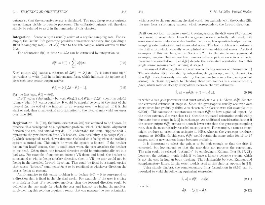
Drift correction To make a useful tracking system, the drift error (9.3) cannotbe allowed to accumulate. Even if the gyroscope were perfectly calibrated, drifterror would nevertheless grow due to other factors such as quantized output values,sampling rate limitations, and unmodeled noise. The first problem is to estimatethe drift error, which is usually accomplished with an additional sensor. Practicalexamples of this will be given in Section 9.2. For the simple merry-go-roundexample, imagine that an overhead camera takes a picture once in a while tomeasure the orientation. Let θd[k] denote the estimated orientation from thissingle sensor measurement, arriving at stage k.

Because of drift error, there are now two conflicting sources of information: 1)The orientation θ[k] estimated by integrating the gyroscope, and 2) the orienta-tion θd[k] instantaneously estimated by the camera (or some other, independentsensor). A classic approach to blending these two sources is a complementaryfilter, which mathematically interpolates between the two estimates:

θc[k] = αθd[k] + (1− α)θ[k], (9.10)

in which α is a gain parameter that must satisfy 0 < α < 1. Above, θc[k] denotesthe corrected estimate at stage k. Since the gyroscope is usually accurate overshort times but gradually drifts, α is chosen to be close to zero (for example, α =0.0001). This causes the instantaneous estimate θd[k] to have a gradual impact. Atthe other extreme, if α were close to 1, then the estimated orientation could wildlyfluctuate due to errors in θd[k] in each stage. An additional consideration is that ifthe sensor output θd[k] arrives at a much lower rate than the gyroscope samplingrate, then the most recently recorded output is used. For example, a camera imagemight produce an orientation estimate at 60Hz, whereas the gyroscope producesoutputs at 1000Hz. In this case, θd[k] would retain the same value for 16 or 17stages, until a new camera image becomes available.

It is important to select the gain α to be high enough so that the drift iscorrected, but low enough so that the user does not perceive the corrections.The gain could be selected “optimally” by employing a Kalman filter [5, 17, 21];however, the optimality only holds if we have a linear stochastic system, whichis not the case in human body tracking. The relationship between Kalman andcomplementary filters, for the exact models used in this chapter, appears in [15].

Using simple algebra, the complementary filter formulation in (9.10) can bereworked to yield the following equivalent expression:

θc[k] = θ[k]− αd[k] (9.11)

in which

d[k] = θd[k]− θ[k]. (9.12)


Figure 9.1: The vibrating MEMS elements respond to Coriolis forces during ro-tation, which are converted into an electrical signal. (Figure by Fabio Pasolini.)

Above, d[k] is just an estimate of the drift error at stage k. Thus, the complemen-tary filter can alternatively be imagined as applying the negated, signed error, bya small, proportional amount α, to try to incrementally force it to zero.

9.2 Tracking 3D Orientation

IMUs Recall from Section 2.1 (Figure 2.9) that IMUs have recently gone fromlarge, heavy mechanical systems to cheap, microscopic MEMS circuits. This pro-gression was a key enabler to high-quality orientation tracking. The gyroscopemeasures angular velocity along three orthogonal axes, to obtain ωx, ωy, and ωz.For each axis, the sensing elements lie in the perpendicular plane, much like thesemicircular canals in the vestibular organ (Section 8.2). The sensing elements ineach case are micromachined mechanical elements that vibrate and operate like atuning fork. If the sensor rotates in its direction of sensitivity, then the elementsexperience Coriolis forces, which are converted into electrical signals. These sig-nals are calibrated to produce an output in degrees or radians per second; seeFigure 9.1.

IMUs usually contain additional sensors that are useful for detecting drift er-rors. Most commonly, accelerometers measure linear acceleration along three axesto obtain ax, ay, and az. The principle of their operation is shown in Figure 9.2.MEMS magnetometers also appear on many modern IMUs, which measure mag-netic field strength along the three perpendicular axis. This is often accomplishedby the mechanical motion of a MEMS structure that is subject to Lorentz forceas it conducts inside of a magnetic field.


(a) (b)

Figure 9.2: (a) A MEMS element for sensing linear acceleration. (b) Due to linearacceleration in one direction, the plates shift and cause a change in capacitanceas measured between the outer plates. (Figure by David Askew.)

Calibration Recall from Section 9.1 that the sensor outputs are distorted dueto calibration issues. In the one-dimensional angular velocity case, there wereonly two parameters, for scale and offset, which appeared in (9.1). In the 3Dsetting, this would naturally extend to 3 scale and 3 offset parameters; however,the situation is worse because there may also be errors due to non-orthogonality ofthe MEMS elements. All of these can be accounted for by 12 parameters arrangedin a homogeneous transform matrix:

ωx

ωy

ωz

1

=

a b c jd e f kg h i ℓ0 0 0 1

ωx

ωy

ωz

1

(9.13)

There are 12 and not 6 DOFs because the upper left, 3-by-3, matrix is not con-strained to be a rotation matrix. The j, k, and ℓ parameters correspond tooffset, whereas all others handle scale and non-orthogonality. Following the samemethodology as in Section 9.1, the inverse of this transform can be estimatedby minimizing the least squares error with respect to outputs of a better sensor,which provides ground truth. The outputs of the MEMS sensor are then adjustedby applying the estimated homogeneous transform to improve performance (thisis an extension of (9.7) to the 12-parameter case). This general methodology ap-plies to calibrating gyroscopes and accelerometers. Magnetometers may also becalibrated in this way, but have further complications such as soft iron bias.

An additional challenge with MEMS sensors is dealing with other subtle de-pendencies. For example, the outputs are sensitive to the particular temperatureof the MEMS elements. If a VR headset heats up during use, then calibrationparameters are needed for every temperature that might arise in practice. Fortu-nately, IMUs usually contain a temperature sensor that can be used to associatethe calibration parameters with the corresponding temperatures. Finally, MEMS


elements may be sensitive to forces acting on the circuit board, which could bechanged, for example, by a dangling connector. Care must be given to isolateexternal board forces from the MEMS circuit.

Integration Now consider the problem converting the sequence of gyroscopeoutputs into an estimate of the 3D orientation. At each stage k a vector

ω[k] = (ωx[k], ωy[k], ωz[k]) (9.14)

arrives from the sensor. In Section 9.1, the sensor output ω[k] was convertedto a change ∆θ[k] in orientation. For the 3D case, the change in orientation isexpressed as a quaternion.

Let q(v, θ) be the quaternion obtained by the axis-angle conversion formula(3.30). Recall from Section 8.1.2 that the instantaneous axis of rotation is themagnitude of the angular velocity. Thus, if ω[k] is the sensor output at stage k,then the estimated rotation axis is

v[k] = ω[k]/‖ω[k]‖. (9.15)

Furthermore, the estimated amount of rotation that occurs during time ∆t is

∆θ[k] = ‖ω[k]‖∆t. (9.16)

Using the estimated rotation axis (9.15) and amount (9.16), the orientation changeover time ∆t is estimated to be

∆q[k] = q(v[k],∆θ[k]). (9.17)

Using (9.17) at each stage, the estimated orientation q[k] after obtaining the latestsensor output is calculated incrementally from q[k − 1] as

q[k] = ∆q[k] ∗ q[k − 1], (9.18)

in which ∗ denotes quaternion multiplication. This is the 3D generalization of(9.9), in which simple addition could be used to combine rotations in the 2D case.In (9.18), quaternion multiplication is needed to aggregate the change in orienta-tion (simple addition is commutative, which is inappropriate for 3D rotations).

Registration The registration problem for the yaw component is the same asin Section 9.2. The forward direction may be chosen from the initial orientationof the rigid body or it could be determined with respect to a fixed direction in theworld. The pitch and roll components should be determined so that they alignwith gravity. The virtual world should not appear to be tilted with respect to thereal world (unless that is the desired effect, which is rarely the case).


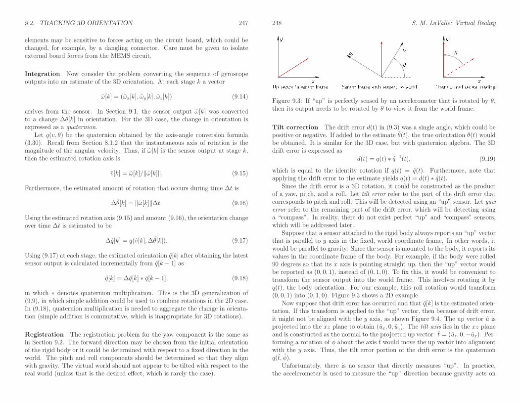
Figure 9.3: If “up” is perfectly sensed by an accelerometer that is rotated by θ,then its output needs to be rotated by θ to view it from the world frame.

Tilt correction The drift error d(t) in (9.3) was a single angle, which could bepositive or negative. If added to the estimate θ(t), the true orientation θ(t) wouldbe obtained. It is similar for the 3D case, but with quaternion algebra. The 3Ddrift error is expressed as

d(t) = q(t) ∗ q−1(t), (9.19)

which is equal to the identity rotation if q(t) = q(t). Furthermore, note thatapplying the drift error to the estimate yields q(t) = d(t) ∗ q(t).

Since the drift error is a 3D rotation, it could be constructed as the productof a yaw, pitch, and a roll. Let tilt error refer to the part of the drift error thatcorresponds to pitch and roll. This will be detected using an “up” sensor. Let yawerror refer to the remaining part of the drift error, which will be detecting usinga “compass”. In reality, there do not exist perfect “up” and “compass” sensors,which will be addressed later.

Suppose that a sensor attached to the rigid body always reports an “up” vectorthat is parallel to y axis in the fixed, world coordinate frame. In other words, itwould be parallel to gravity. Since the sensor is mounted to the body, it reports itsvalues in the coordinate frame of the body. For example, if the body were rolled90 degrees so that its x axis is pointing straight up, then the “up” vector wouldbe reported as (0, 0, 1), instead of (0, 1, 0). To fix this, it would be convenient totransform the sensor output into the world frame. This involves rotating it byq(t), the body orientation. For our example, this roll rotation would transform(0, 0, 1) into (0, 1, 0). Figure 9.3 shows a 2D example.

Now suppose that drift error has occurred and that q[k] is the estimated orien-tation. If this transform is applied to the “up” vector, then because of drift error,it might not be aligned with the y axis, as shown Figure 9.4. The up vector u isprojected into the xz plane to obtain (ux, 0, uz). The tilt axis lies in the xz planeand is constructed as the normal to the projected up vector: t = (uz, 0,−ux). Per-forming a rotation of φ about the axis t would move the up vector into alignmentwith the y axis. Thus, the tilt error portion of the drift error is the quaternionq(t, φ).

Unfortunately, there is no sensor that directly measures “up”. In practice,the accelerometer is used to measure the “up” direction because gravity acts on


(a) (b)

Figure 9.4: (a) Tilt error causes a discrepancy between the y axis and the sensedup vector that is rotated using the estimate q[k] to obtain u. (b) The tilt axis isnormal to u; a rotation of −φ about the tilt axis would bring them into alignment,thereby eliminating the tilt error.

the sensor, causing the sensation of upward acceleration at roughly 9.8m/s2. Theproblem is that it also responds to true linear acceleration of the rigid body, andthis cannot be separated from gravity due to the Einstein equivalence principle. Itmeasures the vector sum of gravity and true linear acceleration, as shown in Figure9.5. A simple heuristic is to trust accelerometer outputs as an estimate of the “up”direction only if its magnitude is close to 9.8m2 [8]. This could correspond to thecommon case in which the rigid body is stationary. However, this assumption isunreliable because downward and lateral linear accelerations can be combined toprovide an output magnitude that is close to 9.8m2, but with a direction that isfar from “up”. Better heuristics may be built from simultaneously considering theoutputs of other sensors or the rate at which “up” appears to change.

Assuming that the accelerometer is producing a reliable estimate of the gravitydirection, the up vector u is calculated from the accelerometer output a by using(3.34), to obtain

u = q[k] ∗ a ∗ q[k]−1. (9.20)

Yaw correction The remaining drift error component is detected by a “com-pass”, which outputs a vector that lies in the world xz plane and always points“north”. Suppose this is n = (0, 0,−1). Once again, the sensor output occursin the coordinate frame of the body, and needs to be transformed by q[k]. Thedifference between n and the −z axis is the resulting yaw drift error.


Gravity Measured accel

Head accel

Gravity

Measured accel

Head accel

(a) (b)

Figure 9.5: (a) There is no gravity sensor; the accelerometer measures the vectorsum of apparent acceleration due to gravity and the true acceleration of the body.(b) A simple heuristic of accepting the reading as gravity only if the magnitudeis approximately 9.8m2 will fail in some cases.

As in the case of the “up” sensor, there is no “compass” in the real world.Instead, there is a magnetometer, which measures a 3D magnetic field vector:(mx, my, mz). Suppose this is used to measure the Earth’s magnetic field. Itturns out that the field vectors do not “point” to the North pole. The Earth’smagnetic field produces 3D vectors that generally do not lie in the horizontalplane, resulting in an inclination angle. Thus, the first problem is that the sensoroutput must be projected into the xz plane. Residents of Ecuador may enjoymagnetic field vectors that are nearly horizontal; however, in Finland they arecloser to vertical; see Figure 9.6. If the magnetic field vector is close to vertical,then the horizontal component may become too small to be useful.

Another issue is that the projected vector in the horizontal plane does notpoint north, resulting in a declination angle; this is the deviation from north.Fortunately, reference to the true north is not important. It only matters that thesensor output is recorded in the registration stage to provide a fixed yaw reference.

The most significant problem is that the magnetometer measures the vectorsum of all magnetic field sources. In addition to the Earth’s field, a buildinggenerates its own field due to ferromagnetic metals. Furthermore, such materialsusually exist on the circuit board that contains the sensor. For this case, thefield moves with the sensor, generating a constant vector offset. Materials thatserve as a source of magnetic fields are called hard iron. Other materials distortmagnetic fields that pass through them; these are called soft iron. Magnetometercalibration methods mainly take into account offsets due to hard-iron bias andeccentricities due to soft-iron bias [12, 20].

After these magnetometer calibrations have been performed, the yaw drift errorcan be estimated from most locations with a few degrees of accuracy, which is suf-ficient to keep yaw errors from gradually accumulating. There are still problems.If a strong field is placed near the sensor, then the readings become dependent onsmall location changes. This could cause the measured direction to change as the


Figure 9.6: The inclination angle of the Earth’s magnetic field vector varies greatlyover the Earth. (Map developed by NOAA/NGDC and CIRES.)

rigid body translates back and forth. Another problem is that in some buildinglocations, vector sum of the Earth’s magnetic field and the field generated by thebuilding could be approximately zero (if they are of similar magnitude and point-ing in opposite directions). In this unfortunate case, the magnetometer cannotproduce useful outputs for yaw drift error detection.

Filtering Using the detected drift error, filtering works in the same way asdescribed in Section 9.1. The complementary filter (9.10) is upgraded to work withquaternions. It becomes slightly more complicated to represent the interpolationin terms of α. Let (v, θ) denote the axis-angle representation of the orientationd[k], which is the estimated drift error (a quaternion value). Let q(v, αθ) representthe quaternion given by axis v and angle αθ. For a small value of α, this can beconsidered as a small step “toward” d[k].

The complementary filter in terms of quaternions becomes

qc[k] = q(v,−αθ) ∗ q[k], (9.21)

which is similar in form to (9.12). The simple subtraction from the 2D case hasbeen replaced above by multiplying an inverse quaternion from the left. Theestimated drift error d[k] is obtained by multiplying the estimated tilt and yawerrors. Alternatively, they could contribute separately to the complementary filter,with different gains for each, and even combined with drift error estimates frommore sources [29].


Yaw Pitch Roll Error+ + + None- + + L/R mix, flipped x+ - + L/R mix, flipped y+ + - L/R mix, flipped z+ - - Inverse and L/R mix, flipped x- + - Inverse and L/R mix, flipped y- - + Inverse and L/R mix, flipped z- - - Inverse

Figure 9.7: A table to help debug common viewpoint transform errors. Each +means that the virtual world appears to move the correct way when performingthe yaw, pitch, or roll. Each − means it moves in the opposite way. The firstcase is correct. All others are bugs. “L/R mix” means that left and right-handedcoordinate systems are getting mixed; the axis that was flipped is indicated.

Setting the viewpoint The viewpoint is set using the estimated orientationq[k], although it might need to be adjusted to account for alternative timings,for the purpose of prediction or image warping, as discussed in Section 7.4. Letq(t) denote the estimated orientation for time t. In terms of the transformationsfrom Section 3.4, we have just estimated Reye. To calculate the correct viewpoint,the inverse is needed. Thus, q−1(t) would correctly transform models to take theestimated viewpoint into account.

A debugging tip Programmers often make mistakes when connecting the trackedorientation to the viewpoint. Figure 9.7 shows a table of the common mistakes.To determine whether the transform has been correctly applied, one should puton the headset and try rotating about the three canonical axes: A pure yaw, apure pitch, and a pure roll. Let + denote that the world is moving correctly withrespect to a head rotation. Let − denote that it seems to move in the oppositedirection. Figure 9.7 shows a table of the eight possible outcomes and the mostlikely cause of each problem.

A head model The translation part of the head motion has not been addressed.Ideally, the head should be the same height in the virtual world as in the real world.This can be handled by the translation part of the Teye matrix (3.36).

We must also account for the fact that as the head rotates, the eyes changetheir positions. For example, in a yaw head movement (nodding “no”), the pupilsdisplace a few centimeters in the x direction. More accurately, they travel alonga circular arc in a horizontal plane. To more closely mimic the real world, themovements of the eyes through space can be simulated by changing the center ofrotation according to a fictitious head model [1]. This trick is needed until Section


Figure 9.8: To obtain a head model, the rotation center is moved so that orientationchanges induce a plausible translation of the eyes. The height h is along the yaxis, and the protrusion p is along the z axis (which leads a negative number).

9.3, where position is instead estimated from more sensors.Recall from Section 3.5 that the cyclopean viewpoint was first considered and

then modified to handle left and right eyes by applying horizontal offsets by insert-ing Tleft (3.50) and Tright (3.52). In a similar way, offsets in the y and z directionscan be added to account for displacement that would come from a rotating head.The result is to insert the following before or after Tright and Tleft:

Thead =

1 0 0 00 1 0 h0 0 1 p0 0 0 1

, (9.22)

in which h is a height parameter and p is a protrusion parameter. See Figure 9.8.The idea is to choose h and p that would correspond to the center of rotationof the head. The parameter h is the distance from the rotation center to theeye height, along the y axis. A typical value is h = 0.15m. The protrusion pis the distance from the rotation center to the cyclopean eye. A typical value isp = −0.10m, which is negative because it extends opposite to the z axis. Usinga fake head model approximates the eye locations as the user rotates her head;however, it is far from perfect. If the torso moves, then this model completelybreaks, resulting in a large mismatch between the real and virtual world headmotions. Nevertheless, this head model is currently used in popular headsets,such as Samsung Gear VR.

An issue also exists with the y height of the head center. The user maybe seated in the real world, but standing in the virtual world. This mismatch


might be uncomfortable. The brain knows that the body is seated because ofproprioception, regardless of the visual stimuli provided by VR. If the user isstanding, then the head-center height could be set so that the eyes are at thesame height as in the real world. This issue even exists for the case of full six-DOF tracking, which is covered next; the user might be sitting, and a verticaloffset is added to make him appear to be standing in VR.

9.3 Tracking Position and Orientation

This section covers tracking of all 6 DOFs for a moving rigid body, with the mostimportant case being head tracking. For convenience, we will refer to the positionand orientation of a body as its pose. Six-DOF tracking enables Teye from 3.4 tobe fully derived from sensor data, rather than inventing positions from a plausiblehead model, as in (9.22). By estimating the position, the powerful depth cue ofparallax becomes much stronger as the user moves her head from side to side. Shecould even approach a small object and look at it from any viewpoint, such asfrom above, below, or the sides. The methods in this section are also useful fortracking hands in space or objects that are manipulated during a VR experience.

Why not just integrate the accelerometer? It seems natural to try to ac-complish 6-DOF tracking with an IMU alone. Recall from Figure 9.5 that theaccelerometer measures the vector sum of true linear acceleration and accelera-tion due to gravity. If the gravity component is subtracted away from the output,as is heuristically accomplished for tilt correction, then it seems that the remainingpart is pure body acceleration. Why not simply integrate this acceleration twiceto obtain position estimates? The trouble is that the drift error rate is much largerthan in the case of a gyroscope. A simple calibration error leads to linearly grow-ing drift error in the gyroscope case because it is the result of a single integration.After a double integration, a calibration error leads to quadratically growing drifterror. This becomes unbearable in practice after a fraction of a second. Further-more, the true body acceleration cannot be accurately extracted, especially whenthe body quickly rotates. Finally, as drift accumulates, what sensors can be usedto estimate the positional drift error? The IMU alone cannot help. Note that itcannot even distinguish motions at constant velocity, including zero motion; thisis the same as our vestibular organs. Despite its shortcomings, modern IMUs re-main an important part of 6-DOF tracking systems because of their high samplingrates and ability to accurately handle the rotational component.

Make your own waves The IMU-based approach to tracking was passive inthe sense that it relied on sources of information that already exist in the envi-ronment. Instead, an active approach can be taken by transmitting waves intothe environment. Since humans operate in the same environment, waves that areperceptible, such as light and sound, are not preferred. Instead, common energy

9.3. TRACKING POSITION AND ORIENTATION 255

1

2

3

(a) (b)

Figure 9.9: The principle of trilateration enables the detector location to be de-termined from estimates of distances to known emitter. A 2D example is shown:(a) from a single emitter, the detector could be anywhere along a circle; (b) usingthree emitters, the position is uniquely determined.

sources in active tracking systems include infrared, ultrasound, and electromag-netic fields.

Consider transmitting an ultrasound pulse (above 20, 000 Hz) from a speakerand using a microphone to listen for its arrival. This is an example of an emitter-detector pair: The speaker is the emitter, and the microphone is the detector.If time measurement is synchronized between source and destination, then thetime of arrival (TOA or time of flight) can be calculated. This is the time thatit took for the pulse to travel the distance d between the emitter and detector.Based on the known propagation speed in the medium (330 m/s for ultrasound),the distance d is estimated. One frustrating limitation of ultrasound systems isreverberation between surfaces, causing the pulse to be received multiple times ateach detector.

When functioning correctly, the position of the detector could then be nar-rowed down to a sphere of radius d, centered at the transmitter; see Figure 9.9(a).By using two transmitters and one microphone, the position is narrowed downto the intersection of two spheres, resulting in a circle (assuming the transmitterlocations are known). With three transmitters, the position is narrowed down totwo points, and with four or more transmitters, the position is uniquely deter-mined.1 The emitter and detector roles could easily be reversed so that the objectbeing tracked carries the emitter, and several receivers are placed around it. Themethod of combining these measurements to determine position is called trilater-ation. If electromagnetic waves, such as radio, light, or infrared, are used insteadof ultrasound, then trilateration could still be applied even though the impossible

1Global positioning systems (GPS) work in this way, but using radio signals, the Earthsurface constraint, and at least one more satellite eliminate time synchronization errors.


(a) (b)

Figure 9.10: (a) A magnetic dipole offers a field that varies its magnitude anddirection as the position changes. (b) The Razer Hydra, a game controller systemthat generates a weak magnetic field using a base station, enabling it to track thecontroller positions.

to measure the propagation time directly. If the transmitter amplitude is knownthen distance can be estimated based on power degradation, rather than TOA.Alternatively, a time-varying signal can be emitted and its reflected phase shiftcan be estimated when the received signal is superimposed onto the transmittedsignal.

If the detectors do not know the precise time that the pulse started, then theycould compare differences in arrival times between themselves; this is called timedifference of arrival (TDOA). The set of possible locations is a hyperboloid insteadof a sphere. Nevertheless, the hyperboloid sheets can be intersected for multipleemitter-detector pairs to obtain the method of multilateration. This was used inthe Decca Navigation System in World War II to locate ships and aircraft. Thisprinciple is also used by our ears to localize the source of sounds, which will becovered in Section 11.3.

Finally, some methods could track position by emitting a complicated field thatvaries over the tracking area. For example, by creating a magnetic dipole, perhapscoded with a signal to distinguish it from background fields, the position andorientation of a body in the field could be estimated in the field; see Figure 9.10(a).This principle was used for video games in the Razer Hydra tracking system in abase station that generated a magnetic field; see Figure 9.10(b). One drawbackis that the field may become unpredictably warped in each environment, causingstraight-line motions to be estimated as curved. Note that the requirements arethe opposite of what was needed to use a magnetometer for yaw correction inSection 9.2; in that setting the field needed to be constant over the tracking area.For estimating position, the field should vary greatly across different locations.


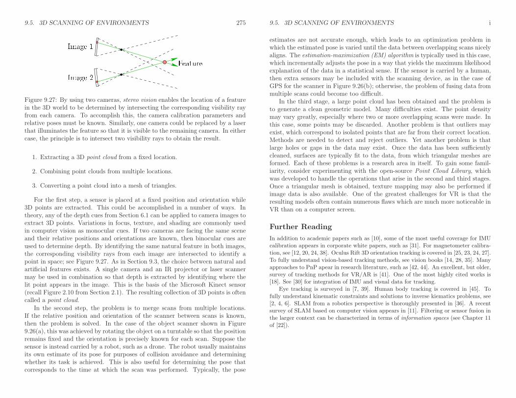
Figure 9.11: The real world contains special features, which are determined to liealong a line segment that connects to the focal point via perspective projection.

The power of visibility The most powerful paradigm for 6-DOF tracking isvisibility. The idea is to identify special parts of the physical world called featuresand calculate their positions along a line-of-sight ray to a known location. Figure9.11 shows an example inspired by a camera, but other hardware could be used.One crucial aspect for tracking is distinguishability. If all features appear to be thesame, then it may become difficult to determine and maintain “which is which”during the tracking process. Each feature should be assigned a unique label thatis invariant over time, as rigid bodies in the world move. Confusing features witheach other could cause catastrophically bad estimates to be made regarding thebody pose.

The most common sensor used to detect features is a digital camera. Detecting,labeling, and tracking features are common tasks in computer vision or imageprocessing. There are two options for features:

1. Natural: The features are automatically discovered, assigned labels, andmaintained during the tracking process.

2. Artificial: The features are engineered and placed into the environment sothat they can be easily detected, matched to preassigned labels, and tracked.

Natural features are advantageous because there are no setup costs. The environ-ment does not need to be engineered. Unfortunately, they are also much moreunreliable. Using a camera, this is considered to be a hard computer vision prob-lem because it may be as challenging as it is for the human visual system. Forsome objects, textures, and lighting conditions, it could work well, but it is ex-tremely hard to make it work reliably for all possible settings. Imagine trying tofind and track features on an empty, white wall. Therefore, artificial features aremuch more common in products.

For artificial features, one of the simplest solutions is to print a special tagonto the object to be tracked. For example, one could print bright red dots onto


Figure 9.12: A sample QR code, which could be printed and used as an artificialfeature. (Picture from Wikipedia.)

Figure 9.13: The Oculus Rift headset contains IR LEDs hidden behind IR-transparent plastic. (Photo by iFixit.)

the object and then scan for their appearance as red blobs in the image. Tosolve the distinguishability problem, multiple colors, such as red, green, blue, andyellow dots, might be needed. Trouble may occur if these colors exist naturally inother parts of the image. A more reliable method is to design a specific tag thatis clearly distinct from the rest of the image. Such tags can be coded to containlarge amounts of information, including a unique identification number. One ofthe most common coded tags is the QR code, an example of which is shown inFigure 9.12.

The features described so far are called passive because they do not emitenergy. The hope is that sufficient light is in the world so that enough reflectsoff of the feature and enters the camera sensor. A more reliable alternative is toengineer active features that emit their own light. For example, colored LEDscan be mounted on the surface of a headset or controller. This comes at theexpense of requiring a power source and increasing overall object cost and weight.Furthermore, its industrial design may be compromised because it might light uplike a Christmas tree.


Cloaking with infrared Fortunately, all of these tricks can be moved to theinfrared (IR) part of the spectrum so that features are visible to cameras, but notto humans. Patterns can be painted onto objects that highly reflect IR energy.Alternatively, IR LEDs can be mounted onto devices. This is the case for theOculus Rift headset, and the IR LEDs are even hidden behind plastic that istransparent for IR energy, but appears black to humans; see Figure 9.13.

In some settings, it might be difficult to mount LEDs on the objects, as inthe case of tracking the subtle motions of an entire human body. This is calledMOCAP or motion capture, which is described in Section 9.4. In MOCAP sys-tems, powerful IR LEDs are positioned around the camera so that they illuminateretroreflective markers that are placed in the scene. Each marker can be imaginedas a spherical mirror in the IR part of the spectrum. One unfortunate drawback isthat the range is limited because IR energy must travel from the camera locationto the target and back again. Since energy dissipates quadratically as a functionof distance, doubling the distance results on one-fourth of the energy level arrivingat the camera.

At this point, it is natural to wonder why an entire image is being capturedif the resulting image processing problem is trivial. The main reason is the pro-liferation of low-cost digital cameras and image processing software. Why notsimply design an emitter-detector pair that produces a binary reading, indicatingwhether the visibility beam is occluded? This is precisely how the detection beamworks in an automatic garage door system to ensure the door does not close onsomeone: An IR LED emits energy to a detection photodiode, which is essentiallya switch that activates when it receives a sufficient level of energy for its targetwavelength (in this case IR). To reduce the amount of energy dissipation, mirrorsor lenses could be used to focus the energy.

Even better, an IR laser can be aimed directly at the detector. The next taskis to use lenses and moving mirrors so that every detector that is visible from afixed location will become illuminated at some point. The beam can be spreadfrom a dot to a line using a lens, and then the line is moved through space usinga spinning mirror. This is the basis of the lighthouse tracking system for the HTCVive headset, which is covered later in this section.

The Perspective-n-Point (PnP) problem A moving rigid body needs to be“pinned down” using n observed features. This is called the Perspective-n-Point(or PnP) problem. We can borrow much of the math from Chapter 3; however,here we consider the placement of bodies in the real world, rather than the virtualworld. Furthermore, we have an inverse problem, which is to determine the bodyplacement based on points in the image. Up until now, the opposite problem wasconsidered. For visual rendering in Chapter 7, an image was produced based onthe known body placement in the (virtual) world.

The features could be placed on the body or in the surrounding world, depend-ing on the sensing method. Suppose for now that they are on the body. Each


Figure 9.14: Each feature that is visible eliminates 2 DOFs. On the left, a singlefeature is visible, and the resulting rigid body has only 4 DOFs remaining. On theright, two features are visible, resulting in only 2 DOFs. This can be visualizedas follows. The edge that touches both segments can be moved back and forthwhile preserving its length if some rotation is also applied. Rotation about anaxis common to the edge provides the second DOF.

feature corresponds to a point p = (x, y, z) with coordinates defined in the frameof the body. Let Trb be a homogeneous transformation matrix that contains thepose parameters, which are assumed to be unknown. Applying the transform Trb

to the point p as in (3.22) could place it anywhere in the real would. Recall thechain of transformations (3.41), which furthermore determines where each pointon the body would appear in an image. The matrix Teye held the camera pose,whereas Tvp and Tcan contained the perspective projection and transformed theprojected point into image coordinates.

Now suppose that a feature has been observed to be at location (i, j) in imagecoordinates. If Trb is unknown, but all other transforms are given, then therewould be six independent parameters to estimate, corresponding to the 6 DOFs.Observing (i, j) provides two independent constraints on the chain of transforms(3.41), one i and one for j. The rigid body therefore loses 2 DOFs, as shown inFigure 9.14. This was the P1P problem because n, the number of features, wasone.

The P2P problem corresponds to observing two features in the image andresults in four constraints. In this case, each constraint eliminates two DOFs,resulting in only two remaining DOFs; see Figure 9.14. Continuing further, if threefeatures are observed, then for the P3P problem, zero DOFs remain (except forthe case in which collinear features are chosen on the body). It may seem that theproblem is completely solved; however, zero DOFs allows for a multiple solutions(they are isolated points in the space of solutions). The P3P problem correspondsto trying to place a given triangle into a pyramid formed by rays so that eachtriangle vertex touches a different ray. This can be generally accomplished infour ways, which are hard to visualize. Imagine trying to slice a tall, thin pyramid(simplex) made of cheese so that four different slices have the exact same triangularsize and shape. The cases of P4P and P5P also result in ambiguous solutions.Finally, in the case of P6P, unique solutions are always obtained if no four featuresare coplanar. All of the mathematical details are worked out in [42].

The PnP problem has been described in the ideal case of having perfect coor-dinate assignments to the feature points on the body and the perfect observationof those through the imaging process. In practice, small errors are made due to


(a) (b)

Figure 9.15: Two cases for camera placement: (a) A world-fixed camera is sta-tionary, and the motions of objects relative to it are estimated using features onthe objects. (b) An object-fixed camera is frequently under motion and featuresare ideally fixed to the world coordinate frame.

factors such as sensor noise, image quantization, and manufacturing tolerances.This results in ambiguities and errors in the estimated pose, which could deviatesubstantially from the correct answer [33]. Therefore, many more features maybe used in practice to improve accuracy. Furthermore, a calibration procedure,such as bundle adjustment [14, 32, 37], may be applied before the device is usedso that the feature point locations can be more accurately assigned before poseestimation is performed. Robustness may be improved by employing RANSAC[9].

Camera-based implementation The visibility problem may be solved usinga camera in two general ways, as indicated in Figure 9.15. Consider the cameraframe, which is analogous to the eye frame from Figure 3.14 in Chapter 3. Aworld-fixed camera is usually stationary, meaning that the camera frame does notmove relative to the world. A single transformation may be used to convert anobject pose as estimated from the camera frame into a convenient world frame.For example, in the case of the Oculus Rift headset, the head pose could beconverted to a world frame in which the −z direction is pointing at the camera,y is “up”, and the position is in the center of the camera’s tracking region ora suitable default based on the user’s initial head position. For an object-fixedcamera, the estimated pose, derived from features that remain fixed in the world,is the transformation from the camera frame to the world frame. This case wouldbe obtained, for example, if QR codes were placed on the walls.

As in the case of an IMU, calibration is important for improving sensing ac-curacy. The following homogeneous transformation matrix can be applied to the


image produced by a camera:

αx γ u0

0 αy v00 0 1

(9.23)

The five variables appearing in the matrix are called intrinsic parameters of thecamera. The αx and αy parameters handle scaling, γ handles shearing, and u0

and v0 handle offset of the optical axis. These parameters are typically estimatedby taking images of an object for which all dimensions and distances have beencarefully measured, and performing least-squares estimation to select the param-eters that reduce the sum-of-squares error (as described in Section 9.1). For awide-angle lens, further calibration may be needed to overcome optical distor-tions (recall Section 7.3).

Now suppose that a feature has been observed in the image, perhaps usingsome form of blob detection to extract the pixels that correspond to it from therest of the image [32, 35]. This is easiest for a global shutter camera becauseall pixels will correspond to the same instant of time. In the case of a rollingshutter, the image may need to be transformed to undo the effects of motion(recall Figure 4.33). The location of the observed feature is calculated as a statisticof the blob pixel locations. Most commonly, the average over all blob pixels isused, resulting in non-integer image coordinates. Many issues affect performance:1) quantization errors arise due to image coordinates for each blob pixel beingintegers; 2) if the feature does not cover enough pixels, then the quantizationerrors are worse; 3) changes in lighting conditions may make it difficult to extractthe feature, especially in the case of natural features; 4) at some angles, two ormore features may become close in the image, making it difficult to separate theircorresponding blobs; 5) as various features enter or leave the camera view, theresulting estimated pose may jump. Furthermore, errors tend to be larger alongthe direction of the optical axis.

Laser-based implementation By designing a special emitter-detector pair,the visibility problem can be accurately solved over great distances. This wasaccomplished by the lighthouse tracking system of the 2016 HTC Vive headset,and the Minnesota scanner from 1989 [34]. Figure 9.16 shows the lighthousetracking hardware for the HTC Vive. The operation of a camera is effectivelysimulated, as shown in Figure 9.17(a).

If the base station were a camera, then the sweeping vertical stripe wouldcorrespond to estimating the row of the pixel that corresponds to the feature;see Figure 9.17(a). Likewise, the sweeping horizontal stripe corresponds to thepixel column. The rotation rate of the spinning drum is known and is analogousto the camera frame rate. The precise timing is recorded as the beam hits eachphotodiode.

Think about polar coordinates (distance and angle) relative to the base station.Using the angular velocity of the sweep and the relative timing differences, the


(a) (b)

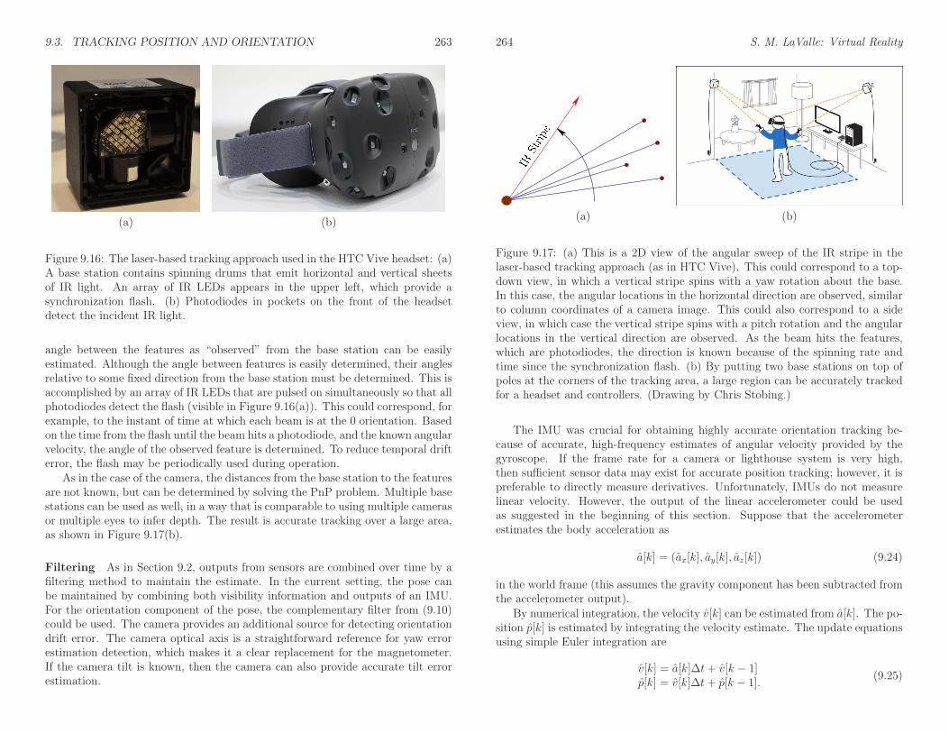
Figure 9.16: The laser-based tracking approach used in the HTC Vive headset: (a)A base station contains spinning drums that emit horizontal and vertical sheetsof IR light. An array of IR LEDs appears in the upper left, which provide asynchronization flash. (b) Photodiodes in pockets on the front of the headsetdetect the incident IR light.

angle between the features as “observed” from the base station can be easilyestimated. Although the angle between features is easily determined, their anglesrelative to some fixed direction from the base station must be determined. This isaccomplished by an array of IR LEDs that are pulsed on simultaneously so that allphotodiodes detect the flash (visible in Figure 9.16(a)). This could correspond, forexample, to the instant of time at which each beam is at the 0 orientation. Basedon the time from the flash until the beam hits a photodiode, and the known angularvelocity, the angle of the observed feature is determined. To reduce temporal drifterror, the flash may be periodically used during operation.

As in the case of the camera, the distances from the base station to the featuresare not known, but can be determined by solving the PnP problem. Multiple basestations can be used as well, in a way that is comparable to using multiple camerasor multiple eyes to infer depth. The result is accurate tracking over a large area,as shown in Figure 9.17(b).

Filtering As in Section 9.2, outputs from sensors are combined over time by afiltering method to maintain the estimate. In the current setting, the pose canbe maintained by combining both visibility information and outputs of an IMU.For the orientation component of the pose, the complementary filter from (9.10)could be used. The camera provides an additional source for detecting orientationdrift error. The camera optical axis is a straightforward reference for yaw errorestimation detection, which makes it a clear replacement for the magnetometer.If the camera tilt is known, then the camera can also provide accurate tilt errorestimation.


(a) (b)

Figure 9.17: (a) This is a 2D view of the angular sweep of the IR stripe in thelaser-based tracking approach (as in HTC Vive). This could correspond to a top-down view, in which a vertical stripe spins with a yaw rotation about the base.In this case, the angular locations in the horizontal direction are observed, similarto column coordinates of a camera image. This could also correspond to a sideview, in which case the vertical stripe spins with a pitch rotation and the angularlocations in the vertical direction are observed. As the beam hits the features,which are photodiodes, the direction is known because of the spinning rate andtime since the synchronization flash. (b) By putting two base stations on top ofpoles at the corners of the tracking area, a large region can be accurately trackedfor a headset and controllers. (Drawing by Chris Stobing.)

The IMU was crucial for obtaining highly accurate orientation tracking be-cause of accurate, high-frequency estimates of angular velocity provided by thegyroscope. If the frame rate for a camera or lighthouse system is very high,then sufficient sensor data may exist for accurate position tracking; however, it ispreferable to directly measure derivatives. Unfortunately, IMUs do not measurelinear velocity. However, the output of the linear accelerometer could be usedas suggested in the beginning of this section. Suppose that the accelerometerestimates the body acceleration as

a[k] = (ax[k], ay[k], az[k]) (9.24)

in the world frame (this assumes the gravity component has been subtracted fromthe accelerometer output).

By numerical integration, the velocity v[k] can be estimated from a[k]. The po-sition p[k] is estimated by integrating the velocity estimate. The update equationsusing simple Euler integration are

v[k] = a[k]∆t+ v[k − 1]p[k] = v[k]∆t+ p[k − 1].

(9.25)

9.4. TRACKING ATTACHED BODIES 265

Note that each equation actually handles three components, x, y, and z, at thesame time. The accuracy of the second equation can be further improved byadding 1

2a[k]∆t2 to the right side.

As stated earlier, double integration of the acceleration leads to rapidly growingposition drift error, denoted by dp[k] . The error detected from PnP solutions

provide an estimate of dp[k], but perhaps at a much lower rate than the IMUproduces observations. For example, a camera might take pictures at 60 FPS andthe IMU might report accelerations at 1000 FPS.

The complementary filter from (9.10) can be extended to the case of doubleintegration to obtain

pc[k] = p[k]− αpdp[k]

vc[k] = v[k]− αvdp[k].(9.26)

Above, pc[k] and vc[k] are the corrected position and velocity, respectively, whichare each calculated by a complementary filter. The estimates p[k] and v[k] are cal-culated using (9.25). The parameters αp and αv control the amount of importancegiven to the drift error estimate in comparison to IMU updates.

Equation (9.26) is actually equivalent to a Kalman filter, which is the opti-mal filter (providing the most accurate estimates possible) for the case of a lineardynamical system with Gaussian noise, and sensors that also suffer from Gaus-sian noise. Let ω2

d represent the variance of the estimated Gaussian noise in thedynamical system, and let ω2

s represent the sensor noise variance. The comple-mentary filter (9.26) is equivalent to the Kalman filter if the parameters are chosenas αp =

√

2ωd/ωs and αv = ωd/ωs [15]. A large variety of alternative filteringmethods exist; however, the impact of using different filtering methods is usuallysmall relative to calibration, sensor error models, and dynamical system mod-els that are particular to the setup. Furthermore, the performance requirementsare mainly perceptually based, which could be different than the classical criteriaaround which filtering methods were designed [26].

Once the filter is running, its pose estimates can be used to aid the PnPproblem. The PnP problem can be solved incrementally by perturbing the poseestimated by the filter, using the most recent accelerometer outputs, so that theobserved features are perfectly matched. Small adjustments can be made to thepose so that the sum-of-squares error is reduced to an acceptable level. In mostcase, this improves reliability when there are so few features visible that the PnPproblem has ambiguous solutions. Without determining the pose incrementally,a catastrophic jump to another PnP solution might occur.

9.4 Tracking Attached Bodies

Many tracking problems involve estimating the motion of one body relative toanother attached, moving body. For example, an eye rotates inside of its socket,which is part of the skull. Although the eye may have six DOFs when treated


(a) (b)

Figure 9.18: (a) The first and sometimes the fourth Purkinje images of an IRlight source are used for eye tracking. (Figure from Wikipedia.) (b) The firstPurkinje image generates a bright reflection as shown. (Picture from MassimoGneo, Maurizio Schmid, Silvia Conforto, and Tomasso D’Alessio.)

as a rigid body in space, its position and orientation are sufficiently characterizedwith two or three parameters once the head pose is given. Other examples includethe head relative to the torso, a hand relative to the wrist, and the tip of a fingerrelative to its middle bone. The entire human body can even be arranged into atree of attached bodies, based on a skeleton. Furthermore, bodies may be attachedin a similar way for other organisms, such as dogs or monkeys, and machinery,such as robots or cars. In the case of a car, the wheels rotate relative to thebody. In all of these case, the result is a multibody system. The mathematicalcharacterization of the poses of bodies relative to each other is called multibodykinematics, and the full determination of their velocities and accelerations is calledmultibody dynamics.

Eye tracking Eye tracking systems been used by vision scientists for over acentury to study eye movements. Three main uses for VR are: 1) To accomplishfoveated rendering, as mentioned in Section 5.4, so that high-resolution renderingneed only be performed for the part of the image that lands on the fovea. 2) Tostudy human behavior by recording tracking data so that insights may be gainedinto VR sickness, attention, and effectiveness of experiences. 3) To render theeye orientations in VR so that social interaction may be improved by offeringeye-contact and indicating someone’s focus of attention; see Section 10.4.

Three general categories of eye-tracking approaches have been developed [7,39]. The first is electro-oculography (EOG), which obtains measurements from sev-eral electrodes placed on the facial skin around each eye. The recorded potentialscorrespond to eye muscle activity, from which the eye orientation relative to the


Revolute Prismatic

Figure 9.19: Two types of 2D joints: A revolute joint allows one link to rotatewith respect to the other, and a prismatic joint allows one link to translate withrespect to the other.

head is determined through filtering. The second approach uses a contact lens,which contains a tiny magnetic coil that causes a potential change in a surround-ing electromagnetic field. The third approach is called video oculography (VOG),which shines IR light onto the eye and senses its corneal reflection using a cameraor photodiodes. The reflection is based on Purkinje images, as shown in Figure9.18. Because of its low cost and minimal invasiveness, this is the most commonlyused method today. The contact lens approach is the most accurate; however, itis also the most uncomfortable.

Forward kinematics Suppose that an eye tracking method has estimated theeye orientation relative to the human skull and it needs to be placed accordinglyin the virtual world. This transformation must involve a combination of the headand eye transforms. For a more complicated problem, consider placing the rightindex finger in the world by using pose of the torso along with all of the anglesformed between bones at each joint. To understand how these and other relatedproblems are solved, it is helpful to first consider 2D examples.

Each body of a multibody system is called a link, and a pair of bodies areattached at a joint, which allows one or more DOFs of motion between them.Figure 9.19 shows two common ways that one planar body might move whileattached to another. The revolute joint is most common and characterizes themotion allowed by a human elbow.

Consider defining a chain of m links, B1 to Bm, and determining the locationof a point on the last link. The points on each link are defined using coordinates ofits own body frame. In this frame, the body appears as shown for Bi−1 in Figure9.20, with the origin at the joint that connects Bi−1 to Bi−2 and the xi−1 axispointing through the joint that connects Bi−1 to Bi. To move the points on Bi to


Figure 9.20: The body frame of each Bi, for 1 < i < m, is based on the jointsthat connect Bi to Bi−1 and Bi+1.

the proper location in the body frame of Bi−1, the homogeneous transform

Ti =

cos θi − sin θi ai−1

sin θi cos θi 00 0 1

. (9.27)

is applied. This rotates Bi by θi, and then translates it along the x axis by ai−1.For a revolute joint, θi is a variable, and ai−1 is a constant. For a prismatic joint,θi is constant and ai−1 is a variable.

Points on Bi are moved into the body frame for B1 by applying the productT2 · · ·Ti. A three-link example is shown in Figure 9.21. To move the first link B1

into the world frame, a general 2D homogeneous transform can be applied:

T1 =

cos θi − sin θi xt

sin θi cos θi yt0 0 1

. (9.28)

This transform is simply added to the matrix product to move each Bi by applyingT1T2 · · ·Ti.

A chain of 3D links is handled in the same way conceptually, but the algebrabecomes more complicated. See Section 3.3 of [22] for more details. Figure 9.22shows six different kinds of joints that are obtained by allowing a pair of 3Dlinks to slide against each other. Each link is assigned a convenient coordinateframe based on the joints. Each homogeneous transform Ti contains a mixture ofconstants and variables in which the variables correspond to the freedom allowedby the joint. The most common assignment scheme is called Denavit-Hartenbergparameters [13]. In some settings, it might be preferable to replace each Ti bya parameterized quaternion that rotates the body, followed by a simple additionthat translates the body.

A tree of links may also be considered; a common example is a human torsoserving as the root, with a head, two arms, and two legs being chains that extend


(a) A three-link chain (b) B3 in its body frame

(c) T3 puts B3 in B2’s body frame (d) T2T3 puts B3 in B1’s body frame

Figure 9.21: Applying the transformation T2T3 to the model of B3. If T1 is theidentity matrix, then this yields the location in the virtual world of points in B3.


Revolute Prismatic Screw1 DOF 1 DOF 1 DOF

Cylindrical Spherical Planar2 DOFs 3 DOFs 3 DOFs

Figure 9.22: Types of 3D joints arising from the 2D surface contact between twobodies.

from it. The human hand is another example. Coordinate frames in this case areoften assigned using Kleinfinger-Khalil parameters [19].

Constraints and inverse kinematics Recall the PnP problem from Section9.3, which involved calculating the pose of a body based on some observed con-straints. A similar problem is to determine the joint parameters for a chain ofbodies by considering the constraints on the bodies. A common example is tocalculate the poses of the arm links by using only the pose of the hand. This isgenerally called the inverse kinematics problem (see [2] and Section 4.4 of [22]).As in the case of PnP, the number of solutions may be infinite, finite, one, orzero. Some 2D examples are shown in Figure 9.23. Generally, if the last link isconstrained, then the freedom of motion for the intermediate links increases as thenumber of links increases. The Chebychev-Grubler-Kutzbach criterion gives thenumber of DOFs, assuming the links are not in some special, singular configura-tions [3]. A common problem in animating video game characters is to maintaina kinematic constraint, such as the hand grasping a doorknob, even though thetorso or door is moving. In this case, iterative optimization is often applied toperturb each joint parameter until the error is sufficiently reduced. The errorwould measure the distance between the hand and the doorknob in our example.


(a) (b)

Figure 9.23: (a) The orientations of both links can be inferred from the position ofthe fixed point; however, there is a second solution if the angles are not restricted.(b) In the case of three links, a one-dimensional family of solutions exists whenthe end is fixed. This can be visualized by pushing down on the top joint, whichwould cause B1 to rotate counter-clockwise. This is equivalent to the classicalfour-bar mechanism, which was used to drive the wheels of a steam engine (thefourth “link” is simply the fixed background).

Motion capture systems Tracking systems for attached bodies use kinematicconstraints to improve their accuracy. The most common application is trackingthe human body, for which the skeleton is well-understood in terms of links andjoints [43]. Such motion capture systems have been an important technologyfor the movie industry as the motions of real actors are brought into a virtualworld for animation. Figure 9.24 illustrates the operation. Features, of the samekind as introduced in Section 9.3, are placed over the body and are visible tocameras mounted around the capture studio. The same options exist for visibility,with the most common approach over the past decade being to use cameras withsurrounding IR LEDs and placing retroreflective markers on the actor.

To obtain a unique pose for each body part, it might seem that six features areneeded (recall P6P from Section 9.3); however, many fewer are sufficient becauseof kinematic constraints. Additional features may nevertheless be used if the goalis to also capture skin motion as it moves along the skeleton. This is especiallyimportant for facial movement. Many new MOCAP technologies are currentlyunder development. For example, a system developed by Noitom captures humanbody movement solely by placing IMUs on the body. Some systems capturemotion by cameras alone, as in the case of Leap Motion (see Figure 9.25) for handtracking, and systems by Microsoft and 8i for full-body tracking by extractingcontours against a green screen. Solutions based on modern depth sensors may


Figure 9.24: With a motion capture (MOCAP) system, artificial features areplaced around the body of a human actor. The motions are extracted and matchedto a kinematic model. Each rigid body in the model has an associated geometricmodel that is rendered to produce the final animated character. (Picture fromWikipedia user Hipocrite.)

also become prevalent in the near future. One challenge is to make highly accurateand reliable systems for low cost and installation effort.

9.5 3D Scanning of Environments

Up until now, this chapter has described how to use sensors to track the motions ofone or more rigid bodies. By contrast, this section describes how sensors are usedto build geometric models of rigid bodies. These could be movable or stationarymodels, as introduced in Section 3.1. A movable model typically correspondsto an object that is be manipulated by the user, such as a sword, hammer, orcoffee cup. These models are often built from a 3D scanner, which images theobject from many viewpoints in a controlled way. The object may be placed on asurface that is surrounded by cameras and other sensors, or it could be placed on aturntable that rotates the object so that it is observed from numerous viewpoints.Alternatively, the sensors may move around while the object remains stationary;

9.5. 3D SCANNING OF ENVIRONMENTS 273

(a) (b)

Figure 9.25: (a) The hand model used by Leap Motion tracking. (b) The trackedmodel superimposed in an image of the actual hands.

see Figure 9.26(a).

SLAM A 3D scanner is useful for smaller objects, with surrounding sensorsfacing inward. For larger objects and stationary models, the sensors are usuallyinside facing out; see Figure 9.26(b). A common example of a stationary modelis the inside of a building. Scanning such models is becoming increasingly im-portant for surveying and forensics. This is also the classical robotics problem ofmapping, in which a robot carrying sensors builds a 2D or 3D representation ofits world for the purposes of navigation and collision avoidance. Robots usuallyneed to estimate their locations based on sensors, which is called the localizationproblem. Robot localization and tracking bodies for VR are fundamentally thesame problems, with the main distinction being that known motion commandsare given to robots, but the corresponding human intent is not directly given.Robots often need to solve mapping and localization problems at the same time,which results in the simultaneous localization and mapping problem; the acronymSLAM is widely used. Due to the similarity of localization, mapping, and VRtracking problems, deep connections exist between robotics and VR. Therefore,many mathematical models, algorithms, and sensing technologies overlap.

Consider the possible uses of a large, stationary model for VR. It could becaptured to provide a virtual world in which the user is placed at the currenttime or a later time. Image data could be combined with the 3D coordinatesof the model, to produce a photorealistic model (recall Figure 2.14 from Section2.2). This is achieved by texture mapping image patches onto the triangles of themodel.


(a) (b)

Figure 9.26: (a) The Afinia ES360 scanner, which produces a 3D model of anobject while it spins on a turntable. (b) The FARO Focus3D X 330 is an outward-facing scanner for building accurate 3D models of large environments; it includesa GPS receiver to help fuse individual scans into a coherent map.

Live capture of the current location Rather than capturing a world in whichto transport the user, sensors could alternatively be used to capture the physicalworld where the user is currently experiencing VR. This allows obstacles in thematched zone to be rendered in the virtual world, which might be useful for safetyor to improve interactivity. For safety, the boundaries of the matched zone couldbe rendered to indicate that the user is about to reach the limit. Hazards such asa hot cup of coffee or a pet walking across the matched zone could be indicated.Interactivity can be improved by bringing fixed objects from the physical worldinto the virtual world. For example, if the user is sitting in front of a desk, thenthe desk can be drawn in the virtual world. If she touches the virtual desk, shewill feel the real desk pushing back. This is a relatively easy way to provide touchfeedback in VR.

Are panoramas sufficient? Before embarking on the process of creating alarge, detailed map of a surrounding 3D world, it is important to consider whetherit is necessary. As mentioned in Section 7.5, panoramic images and videos are be-coming increasingly simple to capture. In some applications, it might be sufficientto build an experience in which the user is transported between panoramas thatwere captured from many locations that are close to each other.

The main ingredients Building a 3D model from sensor data involves threeimportant steps:

9.5. 3D SCANNING OF ENVIRONMENTS 275

Figure 9.27: By using two cameras, stereo vision enables the location of a featurein the 3D world to be determined by intersecting the corresponding visibility rayfrom each camera. To accomplish this, the camera calibration parameters andrelative poses must be known. Similarly, one camera could be replaced by a laserthat illuminates the feature so that it is visible to the remaining camera. In eithercase, the principle is to intersect two visibility rays to obtain the result.

1. Extracting a 3D point cloud from a fixed location.

2. Combining point clouds from multiple locations.

3. Converting a point cloud into a mesh of triangles.

For the first step, a sensor is placed at a fixed position and orientation while3D points are extracted. This could be accomplished in a number of ways. Intheory, any of the depth cues from Section 6.1 can be applied to camera images toextract 3D points. Variations in focus, texture, and shading are commonly usedin computer vision as monocular cues. If two cameras are facing the same sceneand their relative positions and orientations are known, then binocular cues areused to determine depth. By identifying the same natural feature in both images,the corresponding visibility rays from each image are intersected to identify apoint in space; see Figure 9.27. As in Section 9.3, the choice between natural andartificial features exists. A single camera and an IR projector or laser scannermay be used in combination so that depth is extracted by identifying where thelit point appears in the image. This is the basis of the Microsoft Kinect sensor(recall Figure 2.10 from Section 2.1). The resulting collection of 3D points is oftencalled a point cloud.

In the second step, the problem is to merge scans from multiple locations.If the relative position and orientation of the scanner between scans is known,then the problem is solved. In the case of the object scanner shown in Figure9.26(a), this was achieved by rotating the object on a turntable so that the positionremains fixed and the orientation is precisely known for each scan. Suppose thesensor is instead carried by a robot, such as a drone. The robot usually maintainsits own estimate of its pose for purposes of collision avoidance and determiningwhether its task is achieved. This is also useful for determining the pose thatcorresponds to the time at which the scan was performed. Typically, the pose

9.5. 3D SCANNING OF ENVIRONMENTS i

estimates are not accurate enough, which leads to an optimization problem inwhich the estimated pose is varied until the data between overlapping scans nicelyaligns. The estimation-maximization (EM) algorithm is typically used in this case,which incrementally adjusts the pose in a way that yields the maximum likelihoodexplanation of the data in a statistical sense. If the sensor is carried by a human,then extra sensors may be included with the scanning device, as in the case ofGPS for the scanner in Figure 9.26(b); otherwise, the problem of fusing data frommultiple scans could become too difficult.

In the third stage, a large point cloud has been obtained and the problem isto generate a clean geometric model. Many difficulties exist. The point densitymay vary greatly, especially where two or more overlapping scans were made. Inthis case, some points may be discarded. Another problem is that outliers mayexist, which correspond to isolated points that are far from their correct location.Methods are needed to detect and reject outliers. Yet another problem is thatlarge holes or gaps in the data may exist. Once the data has been sufficientlycleaned, surfaces are typically fit to the data, from which triangular meshes areformed. Each of these problems is a research area in itself. To gain some famil-iarity, consider experimenting with the open-source Point Cloud Library, whichwas developed to handle the operations that arise in the second and third stages.Once a triangular mesh is obtained, texture mapping may also be performed ifimage data is also available. One of the greatest challenges for VR is that theresulting models often contain numerous flaws which are much more noticeable inVR than on a computer screen.

Further Reading

In addition to academic papers such as [10], some of the most useful coverage for IMUcalibration appears in corporate white papers, such as [31]. For magnetometer calibra-tion, see [12, 20, 24, 38]. Oculus Rift 3D orientation tracking is covered in [25, 23, 24, 27].To fully understand vision-based tracking methods, see vision books [14, 28, 35]. Manyapproaches to PnP apear in research literature, such as [42, 44]. An excellent, but older,survey of tracking methods for VR/AR is [41]. One of the most highly cited works is[18]. See [30] for integration of IMU and visual data for tracking.

Eye tracking is surveyed in [7, 39]. Human body tracking is covered in [45]. Tofully understand kinematic constraints and solutions to inverse kiematics problems, see[2, 4, 6]. SLAM from a robotics perspective is thoroughly presented in [36]. A recentsurvey of SLAM based on computer vision appears in [11]. Filtering or sensor fusion inthe larger context can be characterized in terms of information spaces (see Chapter 11of [22]).

ii S. M. LaValle: Virtual Reality

Bibliography

[1] Y. Akatsuka and G. A. Bekey. Compensation for end to end delays in a VRsystem. In Proceedings IEEE Virtual Reality Annual International Sympo-sium, pages 156–159, 1998.

[2] J. Angeles. Spatial Kinematic Chains. Analysis, Synthesis, and Optimisation.Springer-Verlag, Berlin, 1982.

[3] J. Angeles. Rotational Kinematics. Springer-Verlag, Berlin, 1989.

[4] J. Angeles. Fundamentals of Robotic Mechanical Systems: Theory, Methods,and Algorithms. Springer-Verlag, Berlin, 2003.

[5] C. K. Chui and G. Chen. Kalman Filtering. Springer-Verlag, Berlin, 1991.

[6] D. Cox, J. Little, and D. O’Shea. Ideals, Varieties, and Algorithms. Springer-Verlag, Berlin, 1992.

[7] A. T. Duchowski. Eye Tracking Methodology: Theory and Practice, 2nd Ed.Springer-Verlag, Berlin, 2007.

[8] J. Favre, B. M. Jolles, O. Siegrist, and K. Aminian. Quaternion-based fu-sion of gyroscopes and accelerometers to improve 3D angle measurement.Electronics Letters, 32(11):612–614, 2006.

[9] M. A. Fischler and R. C. Bolles. Random sample consensus: A paradigm formodel fitting with applications to image analysis and automated cartography.Communications of the ACM, 24(6):381–395, 1981.

[10] W. T. Fong, S. K. Ong, and A. Y. C. Nee. Methods for in-field user calibrationof an inertial measurement unit without external equipment. MeasurementScience and Technology, 19(8), 2008.

[11] J. Fuentes-Pacheco, J. Ruiz-Ascencio, and J. M. Rendon-Mancha. Visualsimultaneous localization and mapping: a survey. Journal Artificial Intelli-gence Review, 43(1):55–81, 2015.

[12] D. Gebre-Egziabher, G. Elkaim, J. David Powell, and B. Parkinson. Cali-bration of strapdown magnetometers in magnetic field domain. Journal ofAerospace Engineering, 19(2):87–102, 2006.

iii

iv BIBLIOGRAPHY

[13] R. S. Hartenberg and J. Denavit. A kinematic notation for lower pair mech-anisms based on matrices. Journal of Applied Mechanics, 77:215–221, 1955.

[14] R. I. Hartley and A. Zisserman. Multiple View Geometry in Computer Vision,2nd Ed. Cambridge University Press, Cambridge, U.K., 2004.

[15] W. T. Higgins. A comparison of complementary and Kalman filtering. IEEETransactions on Aerospace and Electronic Systems, 11(3):321–325, 1975.

[16] A. Iserles. A First Course in the Numerical Analysis of Differential Equa-tions, 2nd Ed. Cambridge University Press, Cambridge, U.K., 2008.

[17] R. Kalman. A new approach to linear filtering and prediction problems.Transactions of the ASME, Journal of Basic Engineering, 82:35–45, 1960.

[18] H. Kato and M. Billinghurst. Marker tracking and hmd calibration for avideo-based augmented reality conferencing system. In Proceedings of IEEEand ACM International Workshop on Augmented Reality, 1999.

[19] W. Khalil and J. F. Kleinfinger. A new geometric notation for openand closed-loop robots. In Proceedings IEEE International Conference onRobotics & Automation, volume 3, pages 1174–1179, 1986.

[20] C. Konvalin. Compensating for tilt, hard-iron, and soft-iron ef-fects. Available at http://www.sensorsmag.com/sensors/motion-velocity-displacement/compensating-tilt-hard-iron-and-soft-iron-effects-6475, Decem-ber 2009. Last retrieved on May 30, 2016.

[21] P. R. Kumar and P. Varaiya. Stochastic Systems. Prentice-Hall, EnglewoodCliffs, NJ, 1986.

[22] S. M. LaValle. Planning Algorithms. Cambridge University Press, Cambridge,U.K., 2006. Available at http://planning.cs.uiuc.edu/.

[23] S. M. LaValle. Help! My cockpit is drifting away. Oculus blog post. Re-trieved from https://developer.oculus.com/blog/magnetometer/, December2013. Last retrieved on Jan 10, 2016.

[24] S. M. LaValle. The latent power of prediction. Oculus blogpost. Retrieved from https://developer.oculus.com/blog/the-latent-power-of-prediction/, July 2013. Last retrieved on Jan 10, 2016.

[25] S. M. LaValle. Sensor fusion: Keeping it simple. Oculus blog post.Retrieved from https://developer.oculus.com/blog/sensor-fusion-keeping-it-simple/, May 2013. Last retrieved on Jan 10, 2016.

[26] S. M. LaValle and P. Giokaris. Perception based predictive tracking for headmounted displays. US Patent 20140354515A1, December 2014.

BIBLIOGRAPHY v

[27] S. M. LaValle, A. Yershova, M. Katsev, and M. Antonov. Head tracking forthe Oculus Rift. In Proc. IEEE International Conference on Robotics andAutomation, pages 187–194, 2014.

[28] Y. Ma, S. Soatto, J. Kosecka, and S. S. Sastry. An Invitation to 3-D Vision.Springer-Verlag, Berlin, 2003.

[29] R. Mahoney, T. Hamel, and J.-M. Pfimlin. Nonlinear complementary filterson the special orthogonal group. IEEE Transactions on Automatic Control,53(5):1203–1218, 2008.

[30] G. Nutzi, S. Weiss, D. Scaramuzza, and R. Siegwart. Fusion of IMU and visionfor absolute scale estimation in monocular SLAM. Journal of Intelligent andRobotic Systems, 61(1):287–299, 2011.

[31] M. Pedley. High-precision calibration of a three-axis accelerome-ter. Technical report, Freescale Semiconductor, 2015. Available athttp://cache.freescale.com/files/sensors/doc/app note/AN4399.pdf.

[32] D. Schmalsteig and T. Hollerer. Augmented Reality: Principles and Practice.Mendeley Ltd., London, 2015.

[33] G. Schweighofer and A. Pinz. Robust pose estimation from a planar tar-get. IEEE Transactions on Pattern Analysis and Machine Intelligence,28(12):2024–2030, 2006.

[34] B. R. Sorensen, M. Donath, G.-B. Yanf, and R. C. Starr. The minnesotascanner: A prototype sensor for three-dimensional tracking of moving bodysegments. IEEE Transactions on Robotics, 5(4):499–509, 1989.

[35] R. Szeliski. Computer Vision: Algorithms and Applications. Springer-Verlag,Berlin, 2010.

[36] S. Thrun, W. Burgard, and D. Fox. Probabilistic Robotics. MIT Press,Cambridge, MA, 2005.

[37] B. Triggs, P. McLauchlan, R. Hartley, and A. Fitzbiggon. Bundle adjustment- a modern synthesis. In Proceedings IEEE International Workshop on VisionAlgorithms, pages 298–372, 1999.

[38] J. F. Vasconcelos, G. Elkaim, C. Silvestre, P. Oliveira, and B. Cardeira.Geometric approach to strapdown magnetometer calibration in sensor frame.Transactions on Aerospace and Electronic Systems, 47(2):1293–1306, 2011.

[39] X. Wang and B. Winslow. Eye tracking in virtual environments. In K. S.Hale and K. M. Stanney, editors, Handbook of Virtual Environments, 2ndEdition. CRC Press, Boca Raton, FL, 2015.

vi BIBLIOGRAPHY

[40] D. S. Watkins. Fundamentals of Matrix Computations. Wiley, Hoboken, NJ,2002.

[41] G. Welch and E. Foxlin. Motion tracking: no silver bullet, but a respectablearsenal. IEEE Computer Graphics and Applications, 22(6):24–28, 2002.

[42] Y. Wu and Z. Hu. PnP problem revisited. Journal of Mathematical Imagingand Vision, 24(1):131–141, 2006.

[43] V. M. Zatsiorsky and B. I. Prilutsky. Biomechanics of Skeletal Muscles.Human Kinetics, Champaign, IL, 2012.

[44] Y. Zheng, Y. Kuang, S. Sugimoto, and K. Astrom. Revisiting the PnP prob-lem: A fast, general and optimal solution. In Proceedings IEEE InternationalConference on Computer Vision, pages 2344–2351, 2013.

[45] H. Zhou and H. Hu. Human motion tracking for rehabilitation - A survey.Biomedical Signal Processing and Control, 3(1):1–18, 2007.

Documents

University of Illinoisvr.cs.uiuc.edu/vrch9.pdf · Available for downloading at http ... dering and display technology requires compensating for the eye ... the calibration produces