Embed Size (px)
Citation preview

UNIVERSITY OF CALIFORNIA
Los Angeles
Analysis of a Feed Bypass Modification
to a Reverse Osmosis System
A thesis submitted in partial satisfaction
of the requirements for the degree Master of Science
in Civil Engineering
by
Richard Newell Franks II
2000

The thesis of Richard Newell Franks II is approved .
Keith D. Stolzenbach
Ivan Catton
Michael K. Stenstrom, Committee Chair
University of California, Los Angeles
2000
ii

Table of Contents
1 .0 Introduction 1
2.0 Review 3
2.1
Reverse Osmosis Defined 3
2.2
Reverse Osmosis Process 5
2.3
Reverse Osmosis Theory 7
2.4 Membrane Performance 8
2.5
Spiral Wound Membrane 9
2.5.1 Design 9
2.5.2 Modifications 12
2.5.3 Adverse Effects 13
3.0
Feed Flow Bypass 16
3 .1
System Modification 16
3.2
Effects of Feed Bypass on System Performance18
3.2.1 Variation on Inlet Flow Rates 18
3.2.2 Variation on Inlet Concentrations 19
4.0
Model Development 21
4.1
Forward Averaging Model Geometry 21
111

4.2
Cell Mass Transport Models 23
4.2.1 Solvent Mass Transport 23
4.2.2 Solute Mass Transport 24
4.2.3 Solution Mass Transport 25
4.3
Cell Permeate Conditions 27
4.4
Cell Exit Conditions 28
4.5
Whole Membrane Solutions 28
4.6
Modifications to Forward Averaging Model34
4.6.1 Spreadsheet 34
4.6.2 System Feed Flow Bypass 34
4.6.3 Brackish Solutions 37
5.0 Results and Discussion 43
5.5 .1 Flow Variations 71
5.5 .2 Membrane Variations 78
iv
5.1 Model Test 43
5.2 Feed Bypass Modeled 51
5.3 Detailed Analysis 57
5.3.1 Analysis of Bypass Flow Rate 57
5.4.2 Bypass Ratios 65
5.5 System Comparison 71

5.6 System Advantages 81
6.0 Conclusions 82
8.0 Appendix 84
9.0 References 85
v

List of Figures
vi

List of Tables
vu

List of Symbols
Ac
high pressure channel cross-sectional area
C
concentration (kg/m 3)
Dab
Diffusivity of Solution (m 2/s)
Dam K/ Z
solute mass transport parameter through membrane (m/s)
H
cell height = high pressure channel height (m)
J
volumetric flux (m3/m2/s)
k
mass transfer coefficient (m/s)
KB
solvent permeability coefficient (m/s/kPa)
KM
mesh step mixing coefficient (m -")
K 9r
osmotic pressure constant (kPa/kg/m3)
L
spiral wound membrane length (m)
N
number of cells per membrane
P
pressure (kPa)
Q
flow rate (m3/s)
S
cell surface area (m)
W
cell width (m)
X
cell length (m)

Greek Symbols
•
change across membrane
7L
osmotic pressure (kPa)
•
solution density (kg/m3)
v
solution kinematic viscosity (m 2/s)
Subscripts
B
solvent
•
exit/reject
mem
whole membrane
•
nth cell
•
inlet of feed
p
permeate
s
solute
sys
reverse osmosis system consisting of one or more spiralwound membranes within a single pressure vessel
w
membrane wall
ix

Acknowledgments
x

ABSTRACT OF THE THESIS
Analysis of a Feed Bypass Modification
to a Reverse Osmosis System
by
Richard Newell Franks II
Master of Science in Civil Engineering
University of California, Los Angeles, 2000
Professor Michael K . Stenstrom, Chair
An analysis was conducted on a proposed reverse osmosis pressure vessel
modification which would allow a portion of the inlet feed flow to bypass the first
membrane and enter subsequent membranes within the same pressure vessel. The
analysis was conducted through the modification of an existing theoretical model using a
spreadsheet program. Whole system response, as well as individual membrane response,
to variations in the quantity of flow diverted past the first membrane was analyzed . The
analysis indicated an increase in recovery would occur in conjunction with a decrease in
separation as flow was diverted past the first membrane and allowed to enter subsequent
membranes .
xi

xii


1.0 Introduction
As world population climbs above six billion, greater stress is placed on the earths
natural resources, especially its limited supply of fresh water . Though climate and
technology influence access to water, the single greatest factor influencing the availability
of existing fresh water is the number of people competing for it (Gardner and Engleman,
1997). The already limited supply of fresh water is itself being diminished by the
contamination that accompanies large scale industrialization, especially in third world
countries .
The environmental threat to a limited water supply, along with a growing demand
for water, necessitates the advancement of water treatment technology . In particular,
there is a need to advance treatment of water by reverse osmosis beyond its present
applications and overcome limitations associated with membrane technology such as
fouling, pressure losses and concentrations polarization . This will most likely be done, as
one author points out, through slow and incremental advances (Simon, 1998) .
A proposed advance would modify the traditional reverse osmosis system, with
spiral wound membranes in series, to allow a portion of the feed flow to bypass the first
membrane within a pressure vessel and enter subsequent membranes within that same
pressure vessel (Chancellor et al., 1998) .
1

The goal of this study is to compare the performance of a traditional reverse
osmosis system with the proposed feed bypass system . The analysis will be performed
theoretically by modifying a model available in the literature to simulate the feed bypass .
The model will be used to determine the system's response to feed bypass as well as
compare the performance of a feed bypass system with that of a traditional system .
2

2.1
Reverse Osmosis Defined
Reverse osmosis (RO) is a solution separation process in which a solvent (usually
water) is passed through a semi permeable membrane while both suspended solids and
solute are retained . The solvent is passed through the membrane by applying a pressure
that overcomes the solutions natural osmotic pressure (Figure 2.1). In the absence of
applied pressure, the pure solvent flow through a semi permeable membrane will be from
the side of lesser concentration to that of greater concentration (Figure2 .2) until osmotic
equilibrium is achieved and the pressure difference between the two sides of the
membrane is equal to the osmotic pressure (Figure 2 .3)(Byrne, 1995 ; Bhattacharyya and
Williams, 1992)
Though the first recorded observation of the osmotic process occurred over 200
years ago, modern RO research began relatively recently in the 1950s at both the
University of California, Los Angeles and the University of Florida (Glater, 1998) . Since
that time, the RO process has been applied in such areas as water/wastewater treatment,
desalination, and mineral recovery . A range of industries such as food and beverage, pulp
and paper, and medical and pharmaceutical, also utilize reverse osmosis .
2.0 Review
3

Applied Pressure
Solvent Flow
Q)10
100a
0;0;0100
a 0 0 0 0 0
Membrane
Figure 2.1 Reverse osmosis process in which the applied pressure forces the solvent through the membraneand leaves behind a more concentrated solution .
Membrane
Figure 2.2 Natural osmosis in which the solvent flows from the side of lesser concentration to that of greaterconcentration .
Osmotic Pressure 00 0 0 0
Membrane
Figure 2.3 Osmotic equilibrium in which the pressure difference between the two sides of the membrane isequal to the osmotic pressure.
4

2.2
Reverse Osmosis Process
Reverse osmosis, illustrated in Figure 2 .4, occurs when a feed solution, with a
given concentration (Co), flows over the membrane surface at a flow rate (Qo) . If the
feed solution pressure (Po) is greater than the solution's osmotic pressure, then solvent
flux (JB) will occur through the membrane in a direction opposite to that of natural
osmosis. Though much less than the solvent flux, a solute flux (Js) occurs which is
dependent on the concentration differential across the membrane surface .
Because only a fraction of the feed flow passes through the membrane, the system
produces two separate effluent flows . The flow which passes through the membrane (Qp)
is termed the permeate and possess a much lower concentration (Cp) than both the
original feed flow and the concentrate flow (Qe), or reject, that remains . As the water
passes through the membrane, it leaves behind a solution with higher concentration at the
membrane wall (Cw). Due to pressure losses in the membrane channel, the concentrate
flow leaving the element will be at a slightly lower pressure (Pe) than the feed pressure .
5

Qo
Co
PO
Pressure vessel
JB
Js
Cw
Membrane
QpCp
Qe-100. Ce
Pe
Figure 2 .4 The reverse osmosis process for a single membrane .
6

2.3 Reverse Osmosis Theory
Though several different specific models have been developed to describe passage
through a membrane (Bhattacharyya, 1992 ), a general theory is described below .
The passage of solvent through the membrane can be described by :
JB = Qp = KB (OP - L Jr)
(2.1)
Where
Q P
= permeate flow rate
S
= membrane surface area
KB
= solvent permeability coefficient
AP = differential pressure across the membrane surface
Air = differential osmotic pressure across the membrane surface
The passage of solute through the membrane can be described by :
Js = Ks ACT
7
(2.2)

Where :
KS
= membrane permeability coefficient for the solute
2
= membrane thickness
AC = differential solute concentration across the membrane
2.4 Membrane Performance
The performance of an RO membrane is usually determined by three parameters :
solvent flux through the membrane, recovery and separation (Winston, 1992) . The
solvent flux is given in Equation (2 .1) . The recovery of a system is its ratio of permeate
flow rate (Qp) to feed flow rate (Qo), given by :
Y = Qp /Qo (2.3)
The separation of a system is an indication of the membrane's ability to reject salts while
allowing for the passage of solvents . Separation is given by :
f = 1 - Co/Cp
(2.4)
Where
8

Co = initial feed concentration
Cp = permeate concentration
2.5 Spiral Wound Membrane
2.5.1 Design
With the emergence of RO technology came four designs to maximize the
efficiency and performance of the membranes . These four designs include : plate-and-
frame, tubular, hollow fiber, and spiral wound membranes . Though modifications have
been made to these four original designs, no new designs have been devised since their
development in the 1960s (Matsuura, 1993) .
The spiral wound membrane (SWM) has emerged as one of the more widely used
designs, partly due to its ability to contain a large membrane area in a relatively small
volume. It is assembled by rolling a rectangular sandwich of two or more membranes,
separated by a permeate carrier, around a central permeate collection tube . The SWM is
then inserted into a pressure vessel to form what will be refered to in this paper as the
spiral wound membrane system or SWM system .
The original designs for a single SWM in a pressure tight container originated
with Merton and Bray of Gulf General Atomic Inc . in 1968 (pat 3,386,583 and pat .
9

3,417,870). Nearly ten years later, Bray submitted pat 4,046,685 describing several
membranes stacked in series within a single pressure vessel (Scott, 1981) . In this system,
a peripheral seal forces the total feed flow to pass longitudinally through each membrane
in series so that the reject from the first membrane becomes the feed for the next
membrane. This configuration allows for more than one membrane to take advantage of
the pressure applied to a single pressure vessel (Figure 2 .5) .
10

Peripheral SealPressure Vessel
Figure 2.5 A traditional spiral wound membrane system. A single pressure vesselcontains one or more spiral wound membranes in series. The peripheral seal preventsflow from bypassing any of the membranes .
1 1

2.5.2 Modifications
The placement of SWMs in series in a single pressure vessel has become the
industry standard with only minor modifications to the pressure vessel flow configuration
since the original Bray design in 1977. One such modification places small slots in the
peripheral seals as well as flow channels on the outer membrane surface . The sole
purpose of the modification is to flush the otherwise dead space between the outer surface
of the membrane and the wall of the pressure vessel (Matsuura, 1993) .
Another substantial modification was developed in the Netherlands (Wessels,
1998) . Though intended for low pressure nano- and ultra-filtration, the design is a
modification of the same fundamental SWM system used for reverse osmosis . In this
modification, feed flow is allowed to enter from both ends of the pressure vessel which is
designed with a slightly larger diameter than membranes so as to allow a portion of the
flow to bypass the first membrane and enter subsequent membranes . The design
modification was shown to have several advantages :
•
A slight increase in permeate flux through the elements occurred when
compared to the traditional design .
• The larger diameter pressure vessels eliminated the dead space between
the membranes and pressure vessel wall thus reducing the contamination
of the membranes .
1 2

•
The membranes were also much easier to insert and remove due to the
larger diameter of the pressure vessel .
2.5.3 Adverse Effects
Despite modifications to SWM system, limitations still exist that prevent the RO
process from becoming a more widely accepted form of water purification, especially for
large scale municipal applications . Several obstacles, including hydraulic pressure losses,
concentration polarization, and fouling, hinder the improved performance of the SWM
system .
Concentration Polarization
Concentration polarization can be defined as an increase in solute concentration at
the membrane wall (relative to the bulk concentration) caused by the convective flow of
solute to the wall being greater than the solute's rate of diffusion away from the wall .
The negative effects of concentration polarization include :
•
A decrease in permeate flow.
•
An increase in solute passage through the membrane .
•
A contributor to fouling (Bhattacharyya and Williams, 1992) .
1 3

Fouling
Fouling is an accumulation of particulate mater on the membrane surface which
results in the plugging of the membrane and therefore a decrease in the permeate flow
(Bhattacharyya and Williams, 1992). Foulants can be classified in three broad categories :
1 . sparingly soluble inorganic compounds,
2. particulate matter, and
3. dissolved organic compounds (Potts et al. 1981) .
To reduce concentration polarization and fouling, SWMs are designed with a
plastic netting inserted between the membrane leafs to increase flow turbulence and thus
increase mixing. The drawback to the increased turbulence is an increase in hydraulic
pressure losses through the length of the membrane .
Hydraulic Pressure Losses
A slight drop in hydraulic pressure occurs as the flow moves through the
concentrate channel of a SWM. This pressure drop, which increases with increasing flow
rate, is caused by viscous drag on the spacers and channel walls, fluid forces on the
spacers, and changes in flow direction (Da Costa et al, 1994). The loss of pressure has
an adverse effect on the membrane performance by reducing solvent flux as is evident
from the previously stated solvent transport equation (Equation 2 .1) .
14

The negative effects produced by a single membrane are compounded as flow
passes through each subsequent membrane in a single pressure vessel . Despite the
decrease in productivity, membranes are placed in series in order to take full advantage of
the available driving pressure (Carnahan, 1999) .
15

3.1
System Modification
A suggested modification to the traditional SWM system alters flow patterns
within the pressure vessel (Chancellor et al ., 1998). The modification diverts a
percentage of feed flow past the first membrane and into subsequent membranes within
the same pressure vessel (Figure 3 .1) . A portion of the diverted flow mixes with the
concentrate of the first membrane and serve as influent to the subsequent membrane .
This process is repeated so that the influent to each membrane (except the first) housed
within a single pressure vessel is a mixture of concentrate from the previous membrane as
well as a portion of the original feed flow .
When compared to the traditional SWM system, the modification, referred to as
the feed bypass system, alters the flow rates and concentrations seen by each membrane.
This alteration of flow rates and concentrations should impact the overall performance of
the system .
3.0 Feed Flow Bypass
16

FeedFlowBypass
Membranes
Figure 3 .1 A feed bypass system. The absence of a peripheral seal on membranes 1 and2 allows for a percentage of the feed flow to bypass the first membrane and entermembranes 2 and 3 .
17
Pressure Vessel
rPermeate
Concentrate

3.2 Effects of Feed Bypass on System Performance
The performance of a traditional SWM system is, to a certain extent, an
optimization problem (Polyakov 1996) . In the same way, the performance of a feed
bypass system is an optimization problem in as much as the diversion of a percentage of
the flow around the first membrane effects the inlet flow and inlet concentration of all
membranes within the module . The variation in flow and concentration seen by each
membrane will have both a positive and negative effect on the overall performance of
those membranes .
3 .2 .1 Variation on Inlet Flow Rates
Flow through a spiral wound membrane has a significant effect on permeate flux
and separation performance. Both permeate flux and separation are indirectly influenced
by the turbulence that accompanies increased flow rate . As mentioned in chapter 2, the
turbulence serves to mix the highly concentrated wall solution with the less concentrated
bulk solution which reduces the effects of concentration polarization and fouling, thus
increasing salt rejection and permeate flux . This same turbulence has the negative effect
of increasing the hydraulic pressure loss along the length of a membrane channel . As
noted in Chapter 2, the drop in pressure leads to a decrease in permeate flux .
The increase in flow through the downstream membranes of a feed bypass system
18

will therefore cause an increase in separation performance of those elements while
effecting permeate flux both positively and negatively . Inversely, the decrease in flow
through the first element will decrease separation while effecting permeate flux both
positively and negatively .
3.2 .2 Variation on Inlet Concentrations
Like flow rate, the solute concentration entering a membrane element effects both
the permeate flux and separation performance of that element . Specifically, an increase
in concentration increases the solutions osmotic pressure which, according to Equation
2.1, decreases solvent flux .
The concentration of the flow entering a membrane element affects the
performance of the membrane by affecting the magnitude of concentration polarization .
The greater the concentration in the flow, the greater the concentration at the membrane
boundary which results in a greater solute flux . In contrast, a decrease in inlet
concentration has been modeled to show an increase in concentration polarization
(Madireddi et al, 1999) . This increase in concentration polarization, caused by the
increase in permeate flux which comes with a lower concentration, finally hinders
separation performance .
Variation in concentration will also effect some forms of fouling . An increase in
19

concentration polarization to the point of solute saturation leads to the precipitation of
certain inorganic molecules which form a gel on the membrane surface (Potts, 1981) .
The changes in flow rates and concentrations associated with a feed bypass system
should impact the performance of the system . The overall performance of a feed bypass
system is analyzed theoretically in Chapter 5 using a forward averaging model .
20

4.0 Model Development
4.1 Forward Averaging Model Geometry
A theoretical comparison was made between the traditional flow configuration
through a pressure vessel containing spiral wound membranes and the feed bypass
configuration. The comparison was based on modifications made to a forward averaging
model for dilute solutions developed by Dickson et al . (1992). The forward averaging
model divides a hypothetical unwound membrane into discrete cells (Figure 4.1) .
Assuming plug flow conditions through any given cell n, the inlet conditions
(flow rate, concentration, and pressure) to cell n are applied to a set of mass transfer,
mass flow, and empirical equations to calculate the permeate and exit conditions from
cell n. The exit conditions are then used as the inlet conditions for cell n+1 (Figure 4.2) .
The inlet conditions for the first cell (n=1) are equivalent to the feed conditions of the
overall membrane while the exit conditions from the last cell (n=final) are equivalent to
the re ect conditions of the overall membrane .
2 1

e
Figure 4.1 Unwound membrane divided into discrete cells for the forwardaveraging model .
Qe (n) = Qo (n+1)Qp (n)
Ce (n) = Co (n+1)Cp (n)
Pe (n) = Po (n+1)
22
Figure 4.2
A single cell n of the forward averaging model .

4.2
Cell Mass Transport Models
Three mass transport models, along with dilute solution assumptions, allow the
permeate conditions leaving cell n to be easily calculated . The three mass transport
models are derived from a generalized capillary flow model developed by Kimura and
Sourira an known as the Kimura-Sourir an Analysis or KSA (Sourira an, 1970) . Each of
the three models and their corresponding simplified equations are discussed below .
4.2.1 Solvent Mass Transport
The first mass transport model gives the following permeate flux for the solvent :
Js = KB (AP - Air) (4.1)
The solvent permeability constant KB , determined experimentally, is specific to both the
membrane and solution .
Two simplifications can be made to Equation (4.1) . First, if the permeate pressure
is atmospheric, then the transmembrane pressure, A P , is equivalent to the inlet pressure,
Po. Second, if the solution is dilute, then the osmotic pressure differential is much less
than the transmembrane pressure and Equation (4.1) can therefore be simplified to :
23

JB = KB (P0)
(4.2)
4.2.2 Solute Mass Transport
The second mass transport model derived from the KSA gives the following
permeate flux for the solute :
Dam KJs =
(CW - Cp)'rP
(4.3)
The solute transport parameter DamK) in Equation (4 .3) is a combination ofz
three separate parameters : solute diffusivity through the membrane (D am ), a factor relating
solute concentration in the membrane to solute concentration in the solution (K), and the
film thickness ( T ). Though it would be difficult to accurately measure each of the three
parameters separately, the combined solute transport parameter can be determined
experimentally .
According to the KSA, Equation (4 .3) can be rewritten in terms of solvent flux if
it is first considered that
24

(JS + JB)
p
and, for dilute solutions,
is + JB = JB
(4.5)
Equation (4.4) then becomes
isJB Cp
P
and Equation (4.3) can be rewritten as
JB _Dam K Cw - Cp
(4.7)T
Cp
4.2.3 Solution Mass Transport
The third mass transport model in the KSA accounts for the concentration
polarization phenomenon and relates the bulk, wall, and permeate concentrations to the
permeate flux of the solution :
25
(4.4)
(4.6)

JB + Js = k In
KM D 213 Q O 1/2
k =
v1/6Ac•2
and Equation (4.8) becomes
26
The mass transfer coefficient k in Equation (4.8) is a function of solute diffusivity,
solution viscosity, flow channel geometry, and feed flow rate. The equation developed by
Dickson for k is based on a mesh step model developed by Winograd et al . (1973) and
results in :
In Equation (4.9), the mesh step mixing coefficient KM is composed of two
constants, the mesh step pitch, M, and the mixing efficiency, Ke, both of which are
functions of spacer geometry within the high pressure flow channel of the spiral wound
membrane.
When a dilute solution is considered then
JS + JB = JB
(4.8)
(4.9)
(4.10)

JB = k InC W
C P
(4.11)(CO -Cp
4.3
Cell Permeate Conditions
The three equations derived from the KSA mass transport models, can be
rearranged and solved simultaneously to determine the permeate conditions for cell n .
Equation (4.2), when multiplied by the surface area of the cell, yields the permeate flow
rate .
The solution to Equations (4 .13) and (4.2) can be used in a rearranged form of Equation
(4.11) to give
Co
CP + 1 -CW
e-c'B/k>
(4.14)CW
CW
27
QP = JB S (4.12)
Equation (4 .7 ) can
C P
be rearranged to give
Dam K/z (4.13)
CW JW + Dam K/Z

Equations (4 .13) and Equation (4.14) can be solved simultaneously to determine the
membrane wall concentration, C, and the permeate concentration, C P , of cell n .
4.4
Cell Exit Conditions
With the newly acquired permeate conditions from cell n, the exit conditions may
now be computed using mass balance equations :
and
Qe = Qo - QP
Co Qo - Cp QpCe =
Qe
(4.15)
(4.16)
The exit pressure from cell n is given by an empirical equation available in the
literature (FilmTec, 1984 as cited by Dickson, 1992 ) :
Pe = Po - [165 x 10 6 (Qo) X]
(4.17)
4.5 Whole Membrane Solutions
As stated before, the final re ect conditions from the whole membrane are equal to
the exit conditions from the last cell . The final permeate conditions, on the other hand,
require some simple calculations. The final permeate flow rate from the whole
28

membrane is the sum of the permeate flow rates from each cell n .
n
Q p(mem) _ 1: Q p(n)
(4.18)
n=1
The final permeate concentration is derived from the permeate flow rates and
concentrations from each cell n .
n
1: Q p(n)C p(n)
C p(mem) = n-(
(4.19)Q p(mem)
Finally, the overall recovery ,Y(mem), and separation, f(mem), of the membrane
can be calculated as :
Y (mem)
f(mem)
Q e(mem)
Q 0(mem)
C O(mem) - C p(mem)
C O(mem)
A summary of the formulas used to calculate the conditions in cell n of the
29
(4.20)
(4.21)
forward averaging model can be found in Table 4 .1 while the necessary model inputs can
be found in Table 4 .2. A flow diagram of the computational procedure is shown in
Figure 4.3 .
30

Table 4.1 Equations for calculating conditions in cell n. Exit conditions from cell n areused as inlet conditions for cell n+l . Equations are presented in the same order that theyare calculated within the forward average algorithm (Figure 4.3) .
3 1
Equation No. Formula
4.9 K M D 2/3 Q 0 1/2
k =
v 1/6 AC 1/2
4.2 JB = KB (Po)
4.13Cp
Dam K/
CW
Dam K/Z
4 .14 Co = Cp +CW
CW1 -
Cp` e -( JB/k)
C,,
4.12 Qp = J,, S
4.17 Pe = Po - [165 x 10 6 (Qo) X]
4.15 Qe = Qo - Qp
4.16 Co Qo - Cp QpCe =
Q e

Table 4.2 Inputs required for the forward averaging model
32
Symbolsconstants
Units DefinitionsSolution
KR m/ s / kPa solvent permeability coefficientV m2/s solution kinematic viscosityD
Membrane constantsm2/s diffusivity
Ac m` high pressure channel cross sectional areaKM m -1/2 mesh step mixing coefficient
DamK/t m/s mass transport parameter across membraneS m2 cell areaX m cell lengthW m channel widthH m channel heightN number of cells per membrane elementL
Flow Conditionsm element length
Qn(mam) inlet feed flowCO(mem) kg/m~ inlet feed concentrationP,,,m ,m) kPa inlet feed pressure

System Wet : Qo(mem), Co(mem), Po(mem)
Read Model Parameters (Table 4 .2)
Yn=n+
Solve Eq . (4.9) to obtain k
VSimultaneously solve Eq. (4.2), (4.13),and (4 .14) to obtain JB, Cw, Cp
YSolve :
To Obtain :
Eq. (4.12)
QpEq. (4.17)
Pe = Po(n+l)Eq. (4.15)
Qe = Qo(n+l)Eq. (4.16)
Ce = Co(n+l)
Yn=n final ?
YesY
Membrane Re ect : Qe(mem) = Qe(n)Ce(mem) = Ce(n)Pe(mem) = Pe(n)
Membrane Permeate : Qp(mem) from Eq. (4.18)Cp(mem) from Eq. (4.19)
Figure 4.3 Computational procedure for the forward averaging model developed byDickson et al.(1992) .
33

4.6 Modifications to Forward Averaging Model
4.6.1 Spreadsheet
Though the forward averaging model was designed for a traditional computer
program, it was easily constructed on a spreadsheet where the computations in Table 4 .1
were performed in a single row on the spreadsheet . Each row on the spreadsheet
corresponded to a cell in the membrane model until the number of rows equaled the
desired number of cells to simulate a single membrane .
The first single membrane (membrane 1) was then copied twice within the same
spreadsheet to create membrane 2 and 3 . The re ect conditions from membrane 1 ( flow
rate, concentration, and pressure) were used as the feed conditions for membrane 2 and
the re ect conditions from membrane 2 were used as the feed conditions for membrane 3 .
The result was the simulation of a reverse osmosis system consisting of three spiral
wound membranes in series within a single pressure vessel (Figure 4 .4) .
4.6.2 System Feed Flow Bypass
To model the flow bypass of membrane 1, the spreadsheet was modified so that a
percentage of the feed flow entering the system could be directed to membranes 2 and 3
as seen in Figure 4 .5 .
34

Qo =Co S =Posr =
Flow
QOM =Co,Y5 =Pogyg =
QO(meml)Co(meml)Po(meml)
Flow -~-)
Membranes
Qe(meml) < Qo(m.2)Ce(meml) > Co (mem2)Pe(meml) = PO (mem2)
35
Pressure Vessel
Qe(mem2) < Qo(mem3)Ce( ) > Co(m.3)Pe(m.2) = Po(m.3)
Membranes
Figure 4.5 The effects of system feed flow bypass on the flow and concentrationentering membranes 1, 2, and 3 in a single pressure vessel . Permeate flow not shown .
Figure 4.4 A traditional reverse osmosis pressure vessel containing three spiral woundmembranes in series . Permeate flow not shown .
Pressure Vessel
Qe(mcm3 )Ce(
)Pe(m,m3)
CQe.== Pe.,> .
QO(meml) Qe(meml) = QO(mem2) Qe(mcm2) = Qo(mem3) Qe(m,.3)CO(meml)PO(meml)
Ce(meml) = Co (mem2)Pe(rl) = Po (mem2)
Ce(m )Pe(m )
= CO(mm3)= Po (mc.3)
Ce(m )Pe(m.3)

The designated percentage of system feed flow entering membrane 2 was added to
the re ect flow of membrane 1 to give the total feed flow entering membrane 2 . For
example, if 10% of the overall system feed flow were designated to enter membrane 2,
then the total feed flow entering membrane 2 would be
Q O(mem2) = 0 .O 1 Q O(sys) + `C e(meml)
A similar calculation was performed to determine the total feed flow entering
membrane 3 .
The ad usted concentrations entering membranes 2 and 3 were derived from mass
flow equations. Using the previous example where 10% of the system feed flow is
designated for membrane 2, the concentration entering membrane 2 would be
(4.21)
C O(mem2) _
0 .0 1 Q O(sys)C 0(sys) + Q e(meml)C e(meml)
0 .0 1 Q O(sys) + Q e(meml)
(4.22)
The effects of system feed flow bypass on the feed pressures of membrane 1 and 2
were considered negligible . For this reason, the feed pressure of each membrane
remained equal to the re ect pressure of the previous membrane .
36

4.6.3 Brackish Solutions
The modified forward averaging model was designed to analyze the performance
of a system treating dilute solutions . For the purposes of this study, it was desirable to
analyze the performance of a system treating brackish solutions where concentrations
would be greater and the effects of osmotic pressure on solvent flux could no longer be
neglected. For analysis of brackish solutions, the osmotic pressure term was included in
the solvent flux equation,
JB = KB (Po - ~r) (4.23)
and the osmotic pressure was computed by multiplying an osmotic pressure constant by
the inlet concentration for any given cell,
it = K r C o
(4.24)
It is important to note that the actual method for computing the osmotic pressure
of sodium chloride solutions involves multiplying an osmotic pressure constant K r of
approximately 79 .3 kPa/kg/m3 (Byrne, 1995) by the wall concentration, not the inlet
concentration . This could not be done in the forward averaging model because the
solvent flux in each cell is computed before the wall concentration is known .
To reduce the error that would arise from using the inlet concentration instead of
37
the wall concentration to compute the solution's osmotic pressure, an amplified osmotic
pressure constant of 275 kPa/kg/m3, was used. The amplified osmotic pressure constant
was derived by trial and error using the outputs from a single membrane in the forward
averaging model and comparing them to data from an actual ROGA-4000 membrane
available in the literature (Ohya and Taniguchi, 1975) . The comparison data used to
obtain an amplified osmotic pressure constant of K ;r = 275 kPa/kg/m3 can be found in
Table 4.3
3 8
Table 4.3 . Comparison of the inputs and outputs from the forward averaging model withpublished ROGA-4000 spiral wound membrane data (Ohya and Taniguchi, 1975) . Thedata was used to obtain an amplified osmotic pressure constant of K x = 275 kPa/kg/m3 .
39
Parameter
Flow Rates (m3/s)
ROGA-4000 Model
Inlet 1 .94 x 10 -4 1 .94 x 10-4
Permeate 2.50 x 10 -5 2.46 x 10⁻⁵
Exit Flow
Concentrations (kg/m3)
Inlet
1 .68 x 10 -4
2 .6
1 .69 x 10"4
2.6
Permeate 0.260 0.297
Exit
Pressures (kPa)
Inlet
2.78
3447.38
2.93
3447.38
Exit 3343.96 3396.75

To test the range of applicability of the derived amplified osmotic pressure
constant, the feed conditions of the forward averaging model were changed to match the
feed conditions of different trials run on the ROGA-4000 . The resulting model outputs,
when compared to outputs of the ROGA-4000 (Table 4.4 and 4.5), show that the forward
averaging model with an amplified osmotic pressure constant of 275 kPa/kg/m3 can
adequately simulate the reverse osmosis process for brackish solutions with flow rates in
the range of 0.0001 - 0.0003 m3/s and concentrations in the range of 2 - 3 kg/m3 . Under
these operating conditions, the model's accuracy was considered sufficient for the
purpose of analyzing the effects of a feed bypass system treating brackish solutions. The
results of the analysis of the feed bypass system treating brackish solutions are discussed
in Chapter 5 .
40

Parameter
Flow Rates (m3/s)
Inlet
Permeate
2.79 x 10⁻⁴
2.6
Exit Flow
Concentrations (kg/m3)
Inlet
Permeate
Exit
Pressures (kPa)
Inlet
Exit
ROGA-4000
3.01 x 10⁻⁴
2.20 x 10⁻⁵
0.260
2.71
2861 .32
2654.48
Model
3.01 x 10⁻⁴
1 .91 x 10' 5
2.82 x 10 -4
2.6
0.245
2.76
2861 .32
2748.45
Table 4.4. Comparison of the forward average model with data from the ROGA-4000spiral wound membrane available in the literature (Ohya and Taniguchi, 1975) to test therange of applicability of the amplified osmotic pressure constant of K ;r = 275kPa/kg/m3 .
4 1
Table 4.5 . Comparison of the forward average model with data from the ROGA-4000spiral wound membrane available in the literature (Ohya and Taniguchi, 1975) to test therange of applicability of the amplified osmotic pressure constant of K x = 275kPa/kg/m3 .
42
Parameter
Flow Rates (m3/s)
Inlet
ROGA-4000
1 .90 x 10-4
Model
1 .90 x 104
Permeate 2.80 x 10⁻⁵ 2.59 x 10⁻⁵
Exit Flow
Concentrations (kg/m3)
Inlet
1 .62 x 10-4
2.1
1 .64 x 10-4
2.1
Permeate 0.198 0.246
Exit
Pressures (kPa)
Inlet
2.12
3447.38
2.39
3447.38
Exit 3309.48 3398.92

5.0 Results and Discussion
5.1
Model Test
Before analyzing the feed bypass system, a traditional system was tested to
determine optimal performance within a range of feed flow rates and concentrations . The
range of flow rates (.000 1 - .0003 m3/s) and the range of concentrations (2 - 3 kg/m3) used
for the test lie within the model's acceptable range for a brackish solution as determined
in Chapter 4. The feed pressure was held constant at 3000 kPa . The test was performed
using parameters for a sodium chloride solution and ROGA-4000 membranes (Table 5.1) .
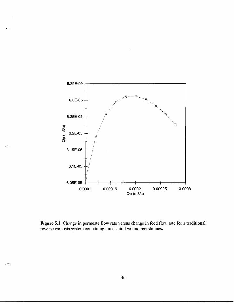
Figures 5 .1 through 5 .5 show the effect on the output of the system when feed rate
and concentration are varied . At the lower feed rates, the effect of concentration
polarization increased the osmotic pressure differential across the membrane which
resulted in a lower permeate flow (Figure 5.1) . As the feed flow increased, the turbulent
mixing reduced the effects of concentration polarization which increased permeate flow .
At some transition point, a maximum was reached and the negative effect of increasing
hydraulic pressure loss (Figure 5 .2) surpassed the positive effects of concentration
polarization reduction and the permeate flow began to decrease once again . The reduction
in concentration polarization that accompanied an increasing flow rate also decreased the
permeate concentration (Figure 5.3) .
43

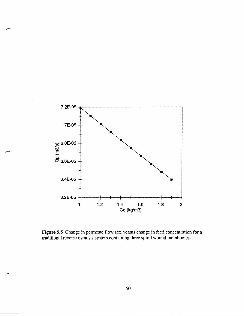
As the inlet concentration increased, the wall concentration increased . This lead
to a greater permeate concentration on the opposite side of the membrane (Figure 5.4) .
The increase in wall concentration also increased the osmotic pressure differential across
the membrane and thus reduced the permeate flow rate (Figure 5 .5) .
In addition to showing the model's response to input variations, the test was used
to set the inlet feed flow rate at 0.003 m3/s for the analysis of a feed flow bypass system .
This feed flow rate would allow the first membrane to approach its optimum performance
as bypass around that membrane was increased .
44
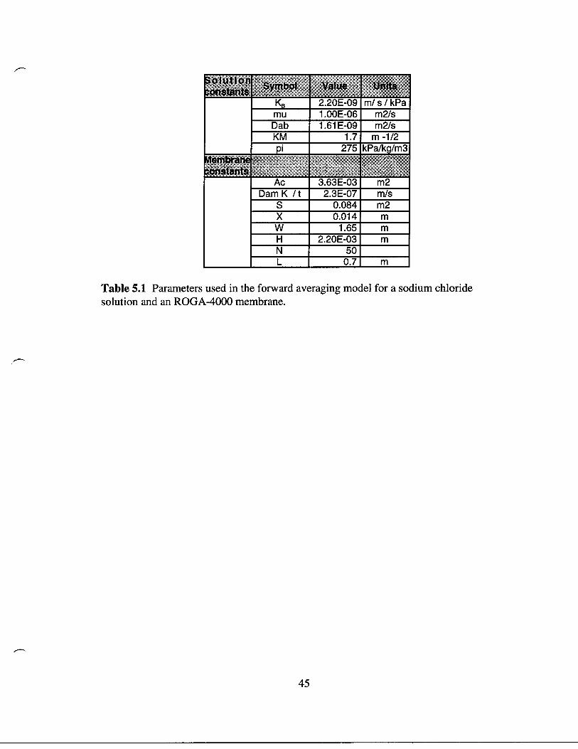
Table 5.1 Para eters used in the forward averaging odel for a sodiu chloridesolution and an ROGA-4000 e brane .
45
Solutionconstants Sy bol
KB
Value
2.20E-09 /
Units
s / kPau 1 .00E-06 2/s
Dab 1 .61 E-09 2/sKM 1 .7 -1/2pi 275 kPa/kq/ 3
Me braneconstants
Ac 3.63E-03 2Da K / t 2.3E-07 /s
S 0.084 2X 0.014W 1 .65H 2.20E-03N 50L 0.7
6.35E-05
6 .05E-05 I0.0001
Figure 5 .1 Change in per eate flow rate versus change in feed flow rate for a traditionalreverse os osis syste containing three spiral wound e branes .
46
IIIi1 a0.00015
0.0002
0.00025
0.0003Qo ( 3/s)

300
250
- 200a
a20150a)Nya)a 100
50
0111#c0.0001
0.00015
0.0002
0.00025
0.0003Qo syste ( 3/s)
Figure 5.2 Change in axial pressure drop versus change in feed flow rate for a traditionalreverse os osis syste containing three spiral wound e branes .
47

0.55
0.5 -
0.45 -
E 0.4 -
0- 0.35-0
0.3 -
0.25 -
0.20.0001
0.00015
0.0002
0.00025
0.0003Qo ( 3/s)
Figure 5 .3 Change in per eate concentration versus change in feed flow rate for atraditional reverse os osis syste containing three spiral wound e branes .
48

0.26
0.24 -
0.22-
00.18-
0.12 11E1111 1
1
1 .2
1 .4
1 .6
1 .8
2Co (kg/ 3)
Figure 5 .4 Change in per eate concentration versus change in feed concentration for atraditional reverse os osis syste containing three spiral wound e branes .
49
6 .2E-05I
I
I1
1 .2
1 .4
1 .6
1 .8
2Co (kg/ 3)
Figure 5.5 Change in per eate flow rate versus change in feed concentration for atraditional reverse os osis syste containing three spiral wound e branes .
50

5.2 Feed Bypass Modeled
After analyzing the perfor ance of a traditional syste , the forward averaging
odel was then used to si ulate a feed bypass syste containing three spiral wound
e branes within a single pressure vessel . A percentage of the feed flow, between 0%
and 40%, was allowed to bypass the first e brane and enter the second and third
e branes at varying ratios . The para eters used were based on a sodiu chloride
solution and the ROGA-4000 e brane (Table 5.1) . The inlet conditions were set at : Qo
= 0.0003 3/s, Co = 2k g/ 3 , and Po = 3000 kPa . The effects on overall syste
recovery, separation and pressure loss where analyzed, the results of which can be viewed
in Figure 5 .6 through 5 .8. Specific values taken fro the figures can be read in Table 5 .2 .
Increasing the a ount of feed flow that bypassed e brane 1 produced a slight
increase in recovery fro 20.63% with no bypass to 21 .42% when the ratio of feed
bypass entering e brane 2 to feed bypass entering e brane 3 was 30/40 in percent
(Figure 5.6). The variation in bypass flow delivered to e brane 3 had a slightly greater
effect on the overall syste recovery than the flow entering e brane two. For exa ple,
if the bypass ratio was set at 40/0, recovery increased to 21 .1 % . If, on the other hand, the
bypass ratio was set at 0/40, the recovery increased to a slightly higher value of 21 .2% .
This slight difference was due, in part, to the higher concentrations seen by e brane 3
that would inevitably be reduced by the bypass entering that e brane .
5 1

The increase in recovery was the result of a significant decrease in the a ount of
pressure lost through the syste (Figure 5 .7) . With no bypass, pressure loss was al ost
300 kPa; but a iniu pressure loss of 125 kPa occurred at a bypass ratio of 40/40 . As
with recovery, the greater effects on pressure loss ca e with variations in the a ount of
flow entering e brane 3 .
With such a significant decrease in the pressure drop through a bypass syste , it
was puzzling to witness a relatively slight increase in recovery . This initial discrepancy is
explained by considering the effects of flow bypass on concentration . As seen in Figure
5.8, a decrease in feed bypass led to a decrease in separation . This decrease in separation
was indicative of an increase in wall concentration which adversely affected recovery .
This pheno enon, along with a ore detailed analysis of the odeled feed bypass syste
and its effect on per eate flux, concentrations, and pressure, is discussed in following
sections .
52

Table 5.2 Syste response to changes in percentage of feed flow bypass diverted toe branes 2 and 3 . Operating conditions are for Qo=0.0003 3/s, Co=2 kg/ 3 , and Po=
3000 kPa. Data is taken fro figures 5.6 through 5 .8 .
53
Inletl Bypass2 Bypass3 Pdrop f YkPa %
100 0 0 294.75 89.77 20.6370 10 20 207.46 88.78 21 .1170 20 10 223.82 89.03 21 .0660 20 20 192.97 88.47 21 .2130 30 40 132.55 85.29 21 .4220 40 40 125.89 82.48 21 .40

Qo = 0.0003 3/sCo = 2 kg/ 3Po = 3000 kPa
0 2 4 6 8 10
15 20 30 40
02
Percentage of feed flowPercentage of feed flow
entering e brane 2entering e brane 3
Figure 5 .6 The effect of varying inlet feed bypass on overall syste recovery .
54

Qo = 0.0003 3/sCo = 2 kg/ 3Po = 3000 kPa
300CO
250a-2000
- 150
0100
a 50La 0
101520304
Percentage of feed flowentering e bane 3
Figure 5.7 The effect of varying inlet feed bypass on overall syste pressure drop .
55
3020
1510
86
4 Percentage of feed flowentering e brane 2

Qo = 0.0003 3/sCo = 2 kg/ 3
Po = 3000 kPa
Percentage of feedentering e brane 2
Figure 5 .8 The effect of varying inlet feed bypass on overall syste separation .
5 6

5.3
Detailed Analysis
The forward averaging odel lent itself to a detailed analysis of the conditions
within the three spiral wound e branes of the pressure vessel . With para eter
conditions and inlet conditions equivalent to those in Table 5 .1, a detailed analysis was
perfor ed on the syste 's response to :
•
A change in flow rate bypassing the first e brane .
•
A change in flow ratio entering the second and third e branes .
5 .3 .1 Analysis of Bypass Flow Rate
A bypass ratio of 0/0 was analyzed to si ulate a traditional syste as the control .
Bypass ratios of 40/40 and 20/20 were analyzed to co pare and contrast the syste 's
response to high and low bypass flow rates . Separation and recovery for a 40/40 and
20/20 bypass syste can be found in Table 5 .2. The variation in flows between the
bypass syste s and the traditional syste can clearly be seen in Figure 5 .8. The spikes in
flows correspond to the location of ixing between two e branes. The higher 40/40
bypass significantly reduced the flow entering the first e brane as well as the pressure
drop through the first and second e branes (Figure 5.9) . The pressure drop through the
third e brane of both bypass syste s was equivalent to the pressure drop through the
third e brane of a traditional syste . Because less pressure was lost through the first
two e branes, the overall pressure loss was significantly less in the bypass syste s .
57

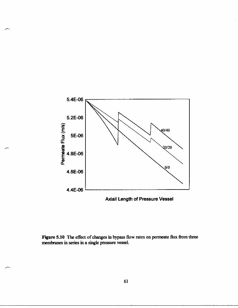
The reduction in pressure loss resulted in greater per eate flux for the 20/20
bypass syste (Figure 5.10). For the 40/40 bypass syste , an increase in concentration
caused the per eate flux through the first e brane to drop below that of the 20/20
bypass and the traditional syste .
The adverse effects of a high feed bypass flow are clearly seen in Figure 5 .11 . A
significant increase in bulk flow concentration occurred in the 40/40 bypass due to the
reduction in cross flow velocity over the e brane surface. As the volu e of water
oving across the e brane surface decreased with unit ti e, the concentration of that
water increased . This increase in bulk flow concentration led to an increase in wall
concentration (Figure 5 .12) which reduced the passage of solvent and increased the
passage of solute (figure 5 .13) .
When the low bypass flow of 20/20 was co pared to the higher bypass flow of
40/40, it beca e clear that the effects of a feed bypass, both positive and negative, were
exaggerated by the higher bypass. This exaggeration ade an i portant difference for
the overall perfor ance of the syste . The lower bypass flow of 20/20 produced solvent
flux values that were co parable to that of the 40/40 bypass, but the 20/20 bypass
produced significantly less per eate concentrations .
58

0.0003
0.00025
0.0002ME
90.00015Mx' 0.0001
5E-05
20/20
0/0
Axial Length of Pressure Vessel
Figure 5.8 Changes in feed bypass flow rates through three e branes in series in asingle pressure vessel .
59

3000
2950
M2900
D..Nc
3 2850N
N
a. 2800
2750
2700
Axial Length of Pressure Vessel
Figure 5.9 The effect of changes in bypass flow rates on pressure through threee branes in series in a single pressure vessel.
60
Axiail Length of Pressure Vessel
Figure 5.10 The effect of changes in bypass flow rates on per eate flux fro threee branes in series in a single pressure vessel .
61
5 .4E-06
5.2E-06
x 5E-06u.
4 .8E-06
0-
4.6E-06
4.4E-06

c-2.8
Y
0 2 .6
C
0 2 .4UY
CO2 .2
Axial Length of Pressure Vessel
Figure 5.11 The effect of changes in bypass flow rates on the bulk concentration of threee branes in series in a single pressure vessel .
62
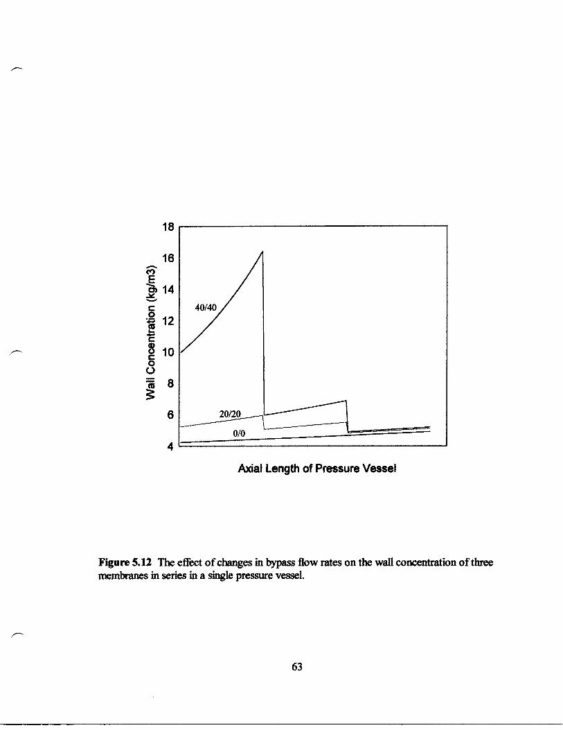
18
16
4
Axial Length of Pressure Vessel
Figure 5.12 The effect of changes in bypass flow rates on the wall concentration of threee branes in series in a single pressure vessel .
63

0.8
0.7E.9 0.6c0
c 0.5
U 0.4
0.3
a~•' 0.2
0.1
Axial Length of Pressure Vessel
Figure 5.13 The effect of change in bypass flow rates on the per eate concentration ofthree e branes in series in a single pressure vessel .
64

5.4.2 Bypass Ratios
It was also desirable to analyze the effects of different ratios on syste
perfor ance. As was entioned in section 5 .2, bypass entering the third e brane had a
greater effect on syste perfor ance when co pared to the bypass entering the second
e brane. Two bypass flow ratios were tested . The ratio of 20/10 allowed greater
bypass flow to enter the second e brane and the ratio of 10/20 allowed for greater
bypass flow to enter the third e brane .
The results indicated that a bypass ratio of 20/10 would lead to slightly better
syste perfor ance. Because the flow rates through the first and third e branes of the
two bypass ratios were very si ilar, if not equivalent, the i prove ent was solely the
result of the increased flow rate through the second e brane (Figure 5 .14). The
increased flow through the second e brane led to a decrease in wall concentration
(Figure 5 .15) and thus a decrease in per eate concentration (Figure 5 .16) .
With a decrease in wall concentration for the second e brane of a 20/10 bypass,
one ight expect the acco panying decrease in os otic pressure to lead to an increase in
per eate flux. But, as pointed out in section 5 .2, the advantages of a decrease in wall
concentration were offset by the increased pressure losses for a 20/10 bypass (Figure
5.17). Per eate flux was only slightly greater for a 10/20 bypass than for a 20/10 bypass
(Figure 5 .18) .
65

0.0003
0 .00028
co 0.00026E
00.00024LL
0.00022
0 .0002
0 .00018
Axial Length of Pressure Vessel
Figure 5.14 The effect of different feed bypass ratios on flow rates through threee branes in series in a single pressure vessel .
66
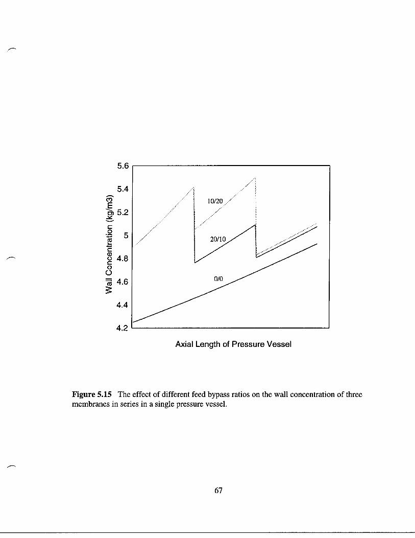
5.6
5 .4COE-0-) 5 .2
c0
CO4-c
5
c 4.80U
4.6
4.4
4 .2
Axial Length of Pressure Vessel
Figure 5.15 The effect of different feed bypass ratios on the wall concentration of threee branes in series in a single pressure vessel .
67

0 .26
ME 0.24
C0
0.22Ca)0CU 0 .2a)4-ct$a)Ea) 0.18
12-
0.16
Axial Length of Pressure Vessel
Figure 5.16 The effect of different feed bypass ratios on the per eate concentration ofthree e branes in series in a single pressure vessel .
68

- 2900a
ME 2850COCOa>
CL 2800
2750
2700
3000
2950
I0/
Axial Length of Pressure Vessel
Figure 5.17 The effect of different feed bypass ratios on the pressure for threee branes in series in a single pressure vessel .
69
10/20
20/

5.4E-06
5.2E-06
NE
x 5E-06U-4-CzE 4.8E-06
a
4.6E-06
4.4E-06
Axiail Length of Pressure Vessel
Figure 5.18 The effect of different feed bypass ratios on the per eate flux through threee branes in series in a single pressure vessel .
70

5.5 Syste Co parison
Using a bypass ratio of 20/10 and the syste para eters found in Table 5.1,
syste perfor ance was analyzed over a range of flowrates and concentrations as well as
for variations in the e brane. The results were co pared with the perfor ance of a
traditional syste .
5 .5 .1 Flow Variations
The effect of changing flow rate on per eate concentration and pressure losses
(Figures 5 .19 and 5.20) was not surprising . The per eate concentration for a 20/10
bypass was slightly higher than the traditional syste at all points in the range tested with
the difference being slightly less at higher flow rates . Pressure losses for a 20/10 bypass
were lower than those of a traditional syste with the difference being slightly less at
lower flow rates .
The effect of changing flow rate on per eate flow was negligible at lower flow
rates. In this range, where wall concentrations beca e very high in both the traditional
syste and the feed bypass syste , the per eate flow dropped off rapidly . In the higher
flow range, the difference between the two syste s beca e uch greater. The feed
bypass syste achieved its opti u per eate flow at a higher inlet flow rate then the
traditional syste (Figure 5.21). This is due in part to the fact that, in the feed bypass
7 1

syste , each of the three e branes approached its opti u per eate flow at si ilar
inlet flow rates (Figure 5 .22) whereas, in a traditional syste , each of the three
e branes achieved opti al per eate flow at slightly different inlet flow rates (Figure
5.23) .
72

0 .2
I
0.0001
0/0
20/10
Figure 5.19 Change in per eate concentration versus change in feed flow rate for thebypass and traditional syste s .
73
I I
0.00015
0.0002
0.00025
0.0003Qo ( 3/s)

0/0 -x- 20/10
Figure 5.20 Change in axil pressure loss versus change in feed flow rate for the bypassand traditional syste s .
74
0 .00015
0.0002
0.00025
0.0003Qo ( 3/s)
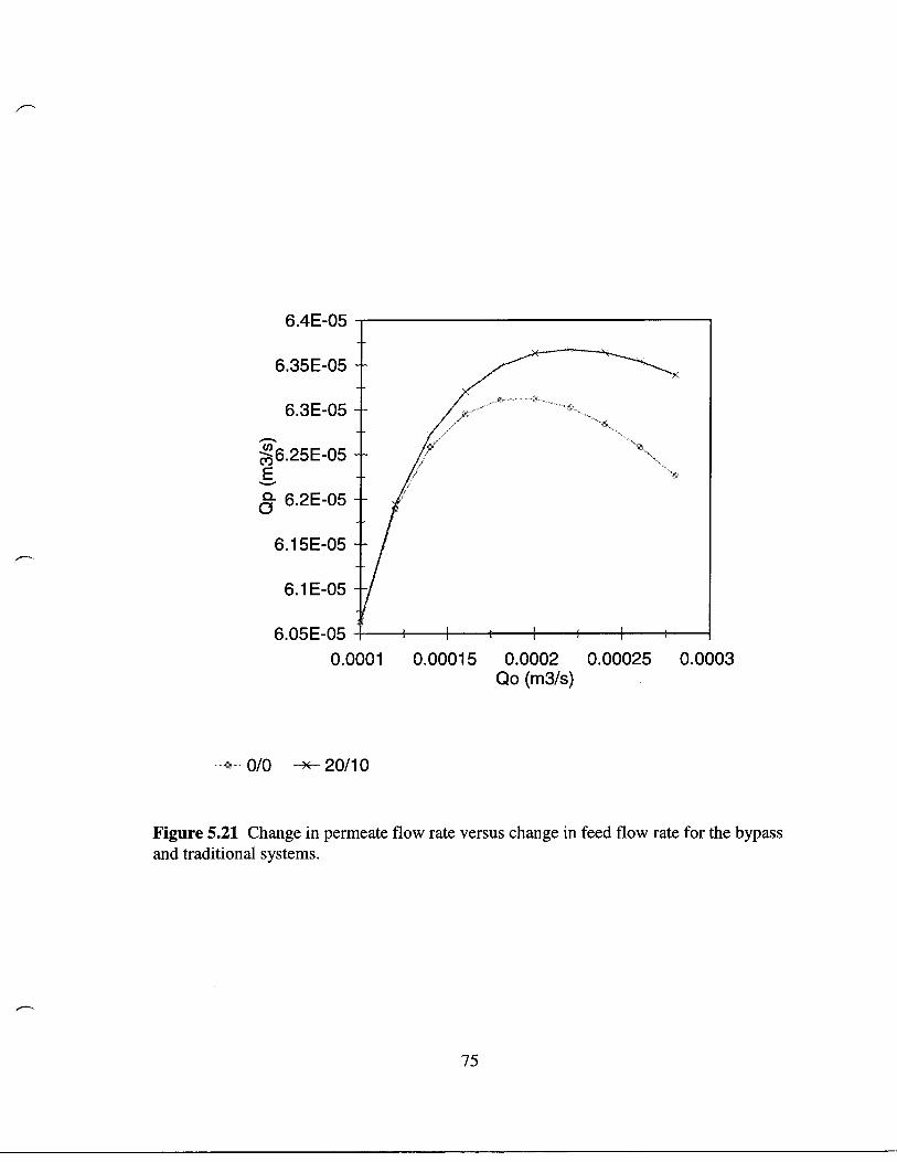
6 .4E-05
6 .35E-05 -
6.3E-05 -
6.25E-05 ---E
6.2E-05 -
6.15E-05 -
6.1 E-05 -
6 .05E-05 -
I
I
i
I II I
0 .0001
0.00015 0.0002 0.00025 0.0003Qo ( 3/s)
-- 0/0
20/10
Figure 5.21 Change in per eate flow rate versus change in feed flow rate for the bypassand traditional syste s .
75

2 .3E-05
2 .2E-05 -
2 .1 E-05 -
M 2E-05 -E -a1 .9E-05 -a
1 .8E-05 -
1 .7E-05 -
1 .6E-05 tI II•I III
0
0.0001 0.0002 0.0003 0 .0004 0 .0005Qo (m3/s)
---- Mem 1 -ae- Mem 2 -w- Mem 3
Figure 5.22 Change in permeate flow rate versus change in feed flow rate for the threemembranes of a bypass system .
76

2 .3E-05
2.2E-05 -
2.1 E-05 -
~. 2E-05 -U)M
~'E 1 .9E-05 -aC~ 1 .8E-05 --
1 .7E-05 -
1 .6E-05 -
Mem 1 -E- Mem 2 -*- Mem 3
Figure 5.23 Change in permeate flow rate versus change in feed flow rate for the threemembranes of a traditional system .
77
1 .5E-05
I tI II II I
0
0.0001 0.0002 0 .0003 0.0004 0.0005Qo (m3/s)

5.5 .2 Membrane Variations
Analyzing the response of feed flow bypass to changes in the membrane size and
structure was limited by the flexibility of the model . For example, changes in channel
thickness returned inconclusive results because the model performs calculations based on
the total cross sectional area, regardless of height and width .
Changes in flow channel width, which translate into changes in membrane size
and therefore changes in cross sectional area, resulted in an increased recovery and a
decrease in separation (Figure 5 .24 and 5.25). The greatest changes occurred in the
system with the greatest feed bypass, suggesting that the effects if a feed bypass system
would be further compounded by employing larger membranes .
78

0.216-
0.214-
0.208-
0.206 I I
1
1 .2
1 .4
1 .6
1 .8
2Channel Width (m)
0/0 -m- 20/10 -- 40/40
Figure 5.24 The effect of changes in membrane size on recovery for different bypassratios .
79

0.92
4-CU
cts 0.86 -0-
(1)
0.84-
0.82-
0.8
1
I
1
C
1
I
I1
1 .2
1 .4
1 .6
1 .8
2Channel Width (m)
: -- 0/0 X11- 20/10 T 40/40
Figure 5.25 The effect of changes in membrane size on separation for different bypassratios .
80

5.6 System dvantages
When considering that the diameter of the spiral wound membrane is less than the
inner diameter of the pressure vessel in a feed bypass system, several advantages over the
traditional system, though not related to the model, should be considered
1 . Because no dead space exists between the outer membrane surface and the inner
wall of the pressure vessel, the outer membrane surface will be flushed and less
fouling will occur .
2 .
The membranes in a feed bypass system are easier to remove and replace which
would lead to a reduction in maintenance costs .
3 .
ecause the feed bypass system does not require specially manufactured pressure
vessels to maintain a seal between the membrane and the vessel wall, overall
system cost could be reduced .
4 .
ecause the bypass system allows flow to both enter and bypass the first
membrane, greater flow per pressure vessel could be treated which would lead to
a reduction in a plant's capital cost .
8 1

6.0 Conclusions
Reverse osmosis is a water treatment technology with the potential to address
current and future water quality challenges on a large scale . Certain restrictions,
including pressure loss, concentration polarization, and fouling, hinder the wider
application of reverse osmosis .
This study uses a forward average model to analyze a propossed modification to
the reverse osmosis process ; the modification allows feed flow to bypass the first
membrane in a pressure vessel and enter subsequent membranes in that same vessel. The
following conclusions were made based on the modeling of a single pressure vessel
containing three spiral wound membranes as well as a general consideration of the
redesign
1 .
Feed flow bypass offers a slight improvement in recovery, a significant reduction
in pressure losses, and a decrease in separation .
2 .
Under the conditions analyzed, the greatest increase in recovery (21 .42%) is
obtained with a bypass ratio of 30/40, while the greatest separation is obtained
with no bypass (a traditional system) .
3 .
slight increase in recovery may still be obtained, but with less of a decrease in
82
separation, by reducing the large buildup of concentration in membranes 1 and 2
that occurs when using a bypass ratio of 30/40 . This is achieved by allowing less
flow to bypass the first membrane and diverting more of that flow to membrane 2
than membrane 3 .
4 .
The feed bypass redesign may also leads to a reduction in fouling on the outer
membrane surface, easier membrane replacement, and an increase in the capacity
of water treated per pressure vessel .
8 3
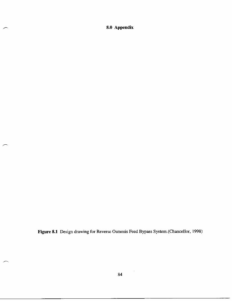
8.0 ppendix
Figure 8 .1 Design drawing for Reverse Osmosis Feed ypass System . ( hancellor, 1998)
84

9.0 References
hattacharyya, . and Williams, M. (1992) . Membrane Handbook, Introduction . Van
Nostrand Reinhold, New York, NY . (edited by Winston, W . and Sirkar, K.) .
yrne, W. (1995) . Reverse Osmosis Practical Guide for Industrial Users . Tall Oaks
Publishing, Littleton, O.
arnahan, R., Graham, W. and Furukawa, . (1999) . "Effects of Flow istribution and
Electromagnetic Fields on Membrane Transport Relationships," International
esalination ssociation Proceedings. San iego, .
hancellor, ., Jensen, J . and Morin O . (1998) . " Revolutionary Gravity ssisted,
Vertical asing, RO emonstration," merican esalting ssociation . Williamsburg,
V .
a osta, ., Fane, . and Wiley, . (1994). "Spacer haracterization and Pressure rop
Modeling in Spacer Filled hannels for Ultrafiltration." Journal of Membrane Science,
87, pp. 79-98 .
ickson, J.M ., Spencer, J. and osta, M.L. (1992). " ilute Single and Mixed Solute
System in a Spiral Wound Reverse Osmosis Module Part 1 Theoretical Model
85

evelopment," esalination, 89, pp . 63-88 .
Gardner, T. and Engleman, R. (1997). Sustaining Water, Easing Scarcity Second
Update, Population in ction International, Washington . .
Glater, J . (1998) . "The Early History of Reverse Osmosis Membrane evelopment,"
esalination, 117, pp . 297-309 .
Lonsdale, H. K. (1982) . "The Growth of Membrane Technology," Journal of Membrane
Science, 10, pp . 81-181 .
Madireddi, K., adcock, R. ., Levine, ., Kim, J.H. and Stenstrom, M. K . (1999) . " n
Unsteady-state Model to Predict oncentration Polarization in ommercial Spiral Wound
Membranes ." Journal of Membrane Science, 157, pp . 13-34 .
Matsuura, T . (1993). Reverse Osmosis Membrane Technology, Water hemistry, and
Industrial pplications . Van Nostrand Reinhold, New York, NY. (Edited by Zahid
mj ad) .
Polyakov, V.S . and Polyakov, S .V . (1996) . "On the alculation of Reverse Osmosis
Plants with Spiral Wound Membrane Elements," esalination, 104, p . 215 .
Porter, M . . (1975) . "Selecting the Right Membrane," hemical Engineering, 71, p. 55 .
86

Potts, .E., hlert, R . . and Wang, S . S . (1981) . " ritical Review of Fouling of
Reverse Osmosis Membranes," esalination, 36, pp. 235-264 .
Ohya, H. and Taniguchi, Y . (1975). " n nalysis of Reveres Osmosis haracteristics of
ROG -4000 Spiral-Wound Module," esalination, 16, pp. 359-373 .
RO System esign with Filmtec Elements (1984) . Technical ulletin, FilmTec
orporation, Minnesota .
Scott, J. (1981) . esalination of Seawater by Reverse Osmosis . Noyes ata orporation,
Park Ridge, New Jersey.
Simon, P. (1998) . Tapped Out, The oming World risis in Water and What We an o
bout It. Welcome Rain, New York .
Sourirajan, 5 . (1970) . Reverse Osmosis . cademic Press, New York, NY .
Sourirajan S . (1977) . Reverse Osmosis and Synthetic Membranes . National Research
ouncil anada Publication, Ottawa, anada.
Wessels, L.P., Van der Meer, W.G.J ., Van Paassen, W. . and Vos, G. (1998) .
87

"Innovative esign of Nano and Ultrafiltration Plants," esalination, 119, pp. 341-345 .
Winograd, Y., Solan, . and Toren, M . (1973) . "Mass Transfer in Narrow hannels in
the Presence of Turbulence Promoters," esalination, 13, pp. 171-186 .
88

ppendix . esign drawing for Reverse Osmosis Feed ypass System . ( hancellor, 1998)
E R SURF E REVERSOSMOSIS T\TSRO)NF'W MO UL RIZE RO SYSTEM
PRO U TION MO ULE
k _--PRESSURE VESSEL
MEM R NE
MEM R NE
P TENT PEN iNGr...... . . .
FIGURE 3
ON ENTR TE ON ENTRI


![IOB (PCB4) - Distrivisa · IOB (PCB4) CN218 [] Duplex/Bypass M:B ... Cntl Paper Feed Clt2:+24V [] Paper Feed Clt2:Contl CN216 S18 CN S19 14 13 12 11 10 9 8 7 6 …](https://img.pdfslide.net/doc/110x75/5ae17dbc7f8b9ab4688ec198/iob-pcb4-distrivisa-pcb4-cn218-duplexbypass-mb-cntl-paper-feed-clt224v.jpg)