UNIVERSITY OF CALIFORNIA Economics 134 DEPARTMENT OF ECONOMICS Spring 2018

Professor David Romer

LECTURE 10

THE ZERO LOWER BOUND IN THE IS-MP-IA FRAMEWORK FEBRUARY 21, 2018

I. INTRODUCTION II. THE IS-MP-IA MODEL EXTENDED A. Assumptions 1. The nominal interest rate can’t be negative 2. Expected inflation depends on actual inflation 3. Discussion B. The AD Curve 1. Where we are headed 2. The IS-MP diagram 3. Deriving the AD curve C. A Little Bit about the Case of Money Targeting III. EXAMPLES A. A Large, Long-Lasting Fall in Planned Expenditure 1. The initial situation 2. The shock 3. Aside: Why doesn’t the AD curve shift left by the same amount at

each inflation rate? 4. The dynamics of the economy 5. What happens when there is a rebound in planned expenditure 6. How seriously should we take this? B. The Case of “Anchored” Expectations 1. Overview 2. A model of anchored expectations 3. The effects of a large, long-lasting fall in planned expenditure 4. A concern: how long can this last?

LECTURE 10 The Zero Lower Bound in the IS-MP-

IA Framework

February 21, 2018

Economics 134 David Romer Spring 2018

Announcements

• Problem Set 2 is being distributed. • It is due at the beginning of lecture a

week from today (Feb. 28). • Optional problem set work session:

Monday, Feb. 26, 6:45–8:15, in 597 Evans Hall.

• A packet of “sample exam questions” is also being distributed.

Announcements (cont.)

• For next time, you do not need to read the paper by Temin and Wigmore.

• My upcoming office hours: • This week: Usual time: Thursday (2/22),

4–5:30. • Next week and the week after: Monday

(2/26 and 3/5), 3:30–5:00.

LECTURE 9 The Conduct of Postwar Monetary Policy

(concluded)

Economics 134 David Romer Spring 2018

Bad Idea: Inflation Responds Little to Slack

Y

π

IA0

AD

π0

Y Y0

IA will shift down only very slowly in response to Y < Y.

IA1 π1

Y

π

AD0

π0

Y�,Y1 Y0 No reason to have Y < Y�. Result: Inflation doesn’t fall.

AD1

What Policies Are Likely to Be Followed If Policymakers Believe Inflation Responds Little to Slack?

IA0

Y

π

AD1

π0

No reason to have Y < Y� believed. Result: Inflation rises. Y�actual Y�believed

What If Policymakers Believe Inflation Responds Little to Slack and Have an Overly Optimistic Estimate of Y�?

IA0

IA1 π1

Y

r

MP1

Fed shifts MP down to get Y = Y� believed. Y�actual Y�believed

If It Is Monetary Policymakers Who Have These Ideas, What Will Be Going on in IS-MP?

IS0

MP0

How Were Ideas Reflected in Monetary Policy Choices in the Early and Late 1970s?

• No reason to for contractionary policy because they thought it wouldn’t curb inflation.

• Unrealistic estimates of the natural rate led to expansionary policy.

• Fed officials pushed for other policies to control inflation, such as price controls.

-5

0

5

10

15

20

Jan-

34

Jan-

37

Jan-

40

Jan-

43

Jan-

46

Jan-

49

Jan-

52

Jan-

55

Jan-

58

Jan-

61

Jan-

64

Jan-

67

Jan-

70

Jan-

73

Jan-

76

Jan-

79

Jan-

82

Jan-

85

Jan-

88

Jan-

91

Jan-

94

Jan-

97

Jan-

00

Jan-

03

Perc

ent

Figure 2 Inflation Rate

Eccles Martin Burns Volcker Greenspan

What Does Romer and Romer’s Analysis Suggest about a Question We Discussed Early in the Course?

• Why did the rise of stabilization policy not cause the economy to quickly become much more stable?

• Romer and Romer’s analysis provides support for the “the tools were used badly” hypothesis.

The Unemployment Rate after “Romer & Romer Dates”

-5

0

5

10

15

20Ja

n-47

May

-49

Sep-

51Ja

n-54

May

-56

Sep-

58Ja

n-61

May

-63

Sep-

65Ja

n-68

May

-70

Sep-

72Ja

n-75

May

-77

Sep-

79Ja

n-82

May

-84

Sep-

86Ja

n-89

May

-91

Sep-

93Ja

n-96

May

-98

Sep-

00Ja

n-03

May

-05

Sep-

07Ja

n-10

Perc

ent

The CPI Inflation Rate after “Romer & Romer Dates”

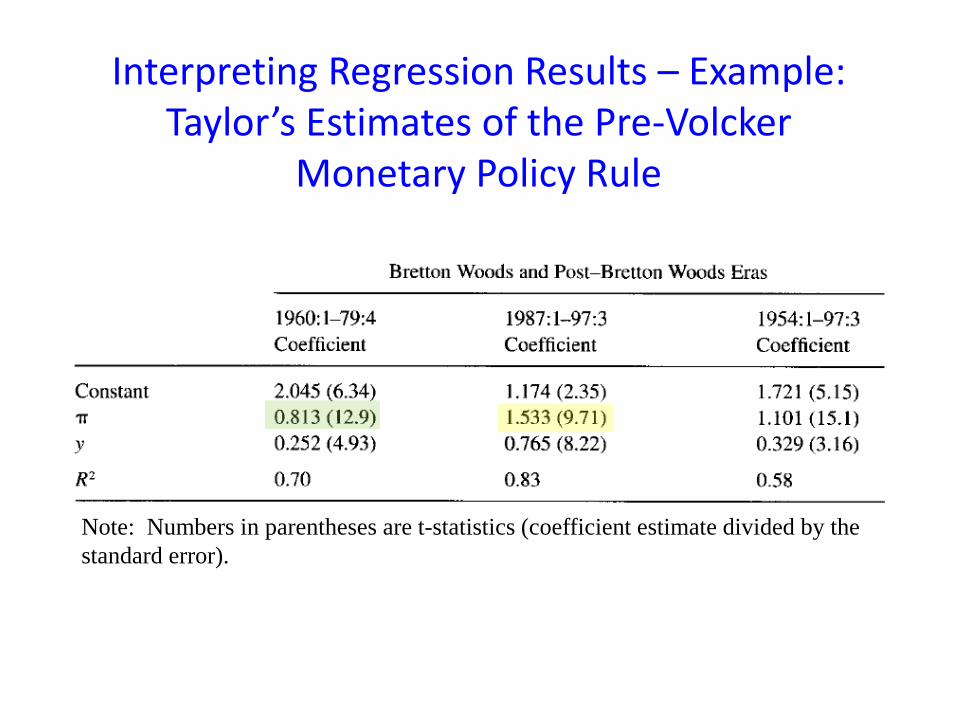
Interpreting Regression Results – Example: Taylor’s Estimates of the Pre-Volcker

Monetary Policy Rule

Note: Numbers in parentheses are t-statistics (coefficient estimate divided by the standard error).

Interpreting Regression Results – Example (cont.)

• For the 1960–1979 sample, Taylor finds a coefficient on inflation = 0.813, with t-statistic = 12.9.

• Since the t-statistic is >> 2, we can reject the hypothesis that the coefficient is 0.

• But what is the 2-standard error confidence interval? Can we reject the hypothesis that the coefficient is 1?

Interpreting Regression Results – Example (cont.) • Coefficient on inflation = 0.813, t-statistic = 12.9.

• t-statistic ≡ coefficient/standard error, so standard error = coefficient/t-statistic.

• So: standard error = 0.813/12.9 = 0.063.

• The two-standard error confidence interval is from 2 standard errors below point estimate to 2 standard errors above.

• So: 2-standard error confidence interval = (0.687,0.939).

• 1 is outside this confidence interval, so we can reject (“at the 5% level”) the hypothesis that the coefficient is 1.

LECTURE 10 The Zero Lower Bound in the IS-MP-

IA Framework

Economics 134 David Romer Spring 2018

I. INTRODUCTION

II. THE IS-MP-IA MODEL EXTENDED

Key Assumptions: 1 The nominal interest rate cannot be negative • The central bank would like to set r = r(Y,π). • Since the real interest rate, r, equals i – πe,

this means that r cannot be less than 0 – πe. • Thus:

−

≥+=

otherwise π00ππ),Y(r if )π,Y(r

re

e

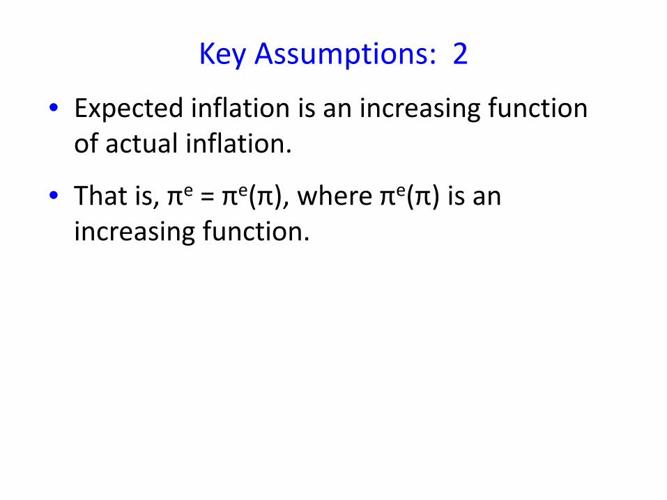
Key Assumptions: 2

• Expected inflation is an increasing function of actual inflation.

• That is, πe = πe(π), where πe(π) is an increasing function.

One Comment Before We Proceed

• We will continue to use the usual IS-MP-IA model (that is, the model without the zero lower bound) in cases where it is appropriate.

Where We Are Headed: The Aggregate Demand Curve Accounting for the Zero Lower Bound

Y

π

AD

The IS and MP Curves Accounting for the Zero Lower Bound: Step 1

Y

r r(Y,π)

0 – πe(π)

IS

The IS and MP Curves Accounting for the Zero Lower Bound: Step 2

Y

r MP

0 – πe(π)

IS

Y

π Y

r Deriving the AD Curve

0 – πe(π0)

MP(π0)

IS0

π0

Y0

Y

π Y

r Deriving the AD Curve

0 – πe(π0)

MP(π0)

IS0

π0

MP(π1)

π1

0 – πe(π1)

MP(π2)

0 – πe(π2)

π2

Y0 Y1 Y2

π0 > π1 > π2

Y

π Y

r Deriving the AD Curve (continued)

IS0

0 – πe(π2)

π2

Y2

MP(π2)

Y

π Y

r Deriving the AD Curve (continued)

IS0

MP(π3)

π2

Y2

π2 > π3

MP(π2)

Y3

π3

0 – πe(π2) 0 – πe(π3)

Deriving the Aggregate Demand Curve: Conclusion

Y

π

AD

A Little Bit about the Case of Money Targeting • Continue to assume that expected inflation is

lower when actual inflation is lower. • Suppose that at some inflation rate, π0, the

nominal interest rate is zero. Thus the real interest rate is 0 – πe(π0).

• Now consider lower inflation, π1 (so π0 > π1). • The lowest possible real interest rate is 0 –

πe(π1), which is higher than the real interest rate at π0, 0 – πe(π0). Thus, r must be higher.

• That is, it is still true that when the economy is at the zero lower bound, lower inflation raises r.

III. EXAMPLES

Y

π Y

r

IS1

MP(π0)

π0, π1

IS0

IA0, IA1

Y0 (= Y) Y1

Y1 Y0 (= Y)

AD0 AD1

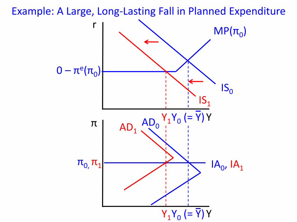
Example: A Large, Long-Lasting Fall in Planned Expenditure

0 – πe(π0)

Y

π AD if r = r(Y,π)

AD if r = 0 – πe(π)

Why Doesn’t the AD Curve Shift Left by the Same Amount at Each Inflation Rate?

Y

r

IS0 IS1

Y1 Y0 Y

r

IS0

0 – πe(π)

IS1

Y1 Y0

r = r(Y,π)

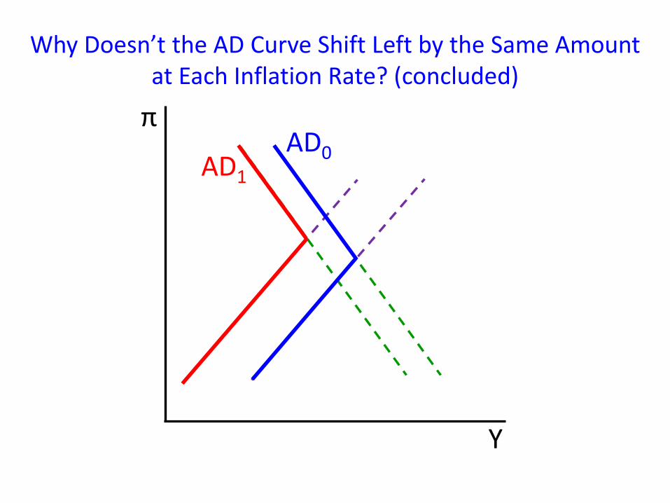
Why Doesn’t the AD Curve Shift Left by the Same Amount at Each Inflation Rate? (continued)

A given shift of the IS curve causes a bigger fall in Y (at a given π) if r = 0 – πe(π) than if r = r(Y,π).

Y

π AD if r = r(Y,π)

AD if r = 0 – πe(π)

Why Doesn’t the AD Curve Shift Left by the Same Amount at Each Inflation Rate? (continued)

Y

π AD0 AD1

Why Doesn’t the AD Curve Shift Left by the Same Amount at Each Inflation Rate? (concluded)

Y

π Y

r

IS1

MP(π1)

0 – πe(π1)

π1

IA1

Y2

AD1

MP(π2)

Y1

IA2 π2

Y

A Large, Long-Lasting Fall in Planned Expenditure (cont.)

0 – πe(π2) Note: Because inflation does not respond immediately to shocks, π1 = π0 (and so IA1 is the same as IA0).

Y

π Y

r

IS1

Y2

AD1

MP(π2) 0 – πe( π2)

IA2 π2

Y

The Effects of a Large Rebound in Planned Expenditure

IS3

Y4

AD3

How Seriously Should We Take This? The main message, which we should take very seriously: When the economy is at the zero lower bound, a key force keeping the economy stable is inoperative.

Inflation fell less in the Great Recession and the (subsequent period of continued high unemployment) than in previous recessions.

Example 2: Anchored Expectations

Two influences on inflation:

• As usual, below-normal output acts to make firms raise price and wages by less than before. This works to push inflation down.

• Firms’ expectations of inflation act to move inflation toward π*. When actual inflation is below π*, this works to push inflation up.

A Model of Anchored Expectations

Y

π Y

r Revisiting a Large, Long-Lasting Fall in Planned Expenditure

MP(π*)

0 – πe(π*)

π*

IS0

IA0

Y0 (= Y)

Y0 (= Y)

AD0

Y

π Y

r

IS1

MP(π*)

π*

IA1

AD1

Y1 Y

A Large, Long-Lasting Fall in Planned Expenditure (cont.)

0 – πe(π*)

With anchored expectations, inflation can stabilize at a level below π* where the upward pull from π* and the downward pull from Y – Y < 0 balance.

A Large, Long-Lasting Fall in Planned Expenditure (concluded)

_