UNIVERSITY OF CALIFORNIA, IRVINE Functional Veriﬁcation …sabdi/SA_thesis.pdfList of Figures vii Acknowledgments ix Curriculum Vitae x Abstract of the Dissertation xii ... 2005

UNIVERSITY OF CALIFORNIA,IRVINE

Functional Verification of System Level Model Refinements

DISSERTATION

submitted in partial satisfaction of the requirementsfor the degree of

DOCTOR OF PHILOSOPHY

in Information and Computer Science

by

Samar Abdi

Dissertation Committee:Professor Daniel D. Gajski, Chair

Professor Ian G. HarrisProfessor Rainer DoemerProfessor Tony Givargis

2005

c© 2005 Samar Abdi

The dissertation of Samar Abdiis approved and is acceptable in qualityand form for publication on microfilm:

Committee Chair

University of California, Irvine2005

ii

DEDICATION

To my parents

iii

Contents

List of Figures vii

Acknowledgments ix

Curriculum Vitae x

Abstract of the Dissertation xii

1 Introduction 11.1 Traditional System Verification . . . . . . . . . . . . . . . . . . . .. . . . . . . 2

1.1.1 Pin and Cycle Accurate Simulation . . . . . . . . . . . . . . . . .. . . 31.1.2 Transaction Level Simulation . . . . . . . . . . . . . . . . . . . .. . . 5

1.2 Proposed System Verification . . . . . . . . . . . . . . . . . . . . . . .. . . . . 61.2.1 System Design Methodology . . . . . . . . . . . . . . . . . . . . . . .. 61.2.2 Formal Modeling . . . . . . . . . . . . . . . . . . . . . . . . . . . . . . 71.2.3 Verification by Correct Refinement . . . . . . . . . . . . . . . . .. . . 7

1.3 Thesis organization . . . . . . . . . . . . . . . . . . . . . . . . . . . . . .. . . 8

2 System Verification Techniques 92.1 Simulation based Methods . . . . . . . . . . . . . . . . . . . . . . . . . .. . . 10

2.1.1 Stimulus Optimization . . . . . . . . . . . . . . . . . . . . . . . . . .. 112.1.2 Monitor Optimization . . . . . . . . . . . . . . . . . . . . . . . . . . . 122.1.3 Speed up techniques . . . . . . . . . . . . . . . . . . . . . . . . . . . . 122.1.4 Modeling Techniques . . . . . . . . . . . . . . . . . . . . . . . . . . . .13

2.2 Formal Verification Methods . . . . . . . . . . . . . . . . . . . . . . . .. . . . 142.2.1 Logic Equivalence Checking . . . . . . . . . . . . . . . . . . . . . .. . 142.2.2 FSM Equivalence Checking . . . . . . . . . . . . . . . . . . . . . . . .152.2.3 Model Checking . . . . . . . . . . . . . . . . . . . . . . . . . . . . . . 172.2.4 Theorem Proving . . . . . . . . . . . . . . . . . . . . . . . . . . . . . . 192.2.5 Drawbacks of Formal Verification . . . . . . . . . . . . . . . . . .. . . 222.2.6 Improvements to Formal Verification Methods . . . . . . . .. . . . . . 222.2.7 Semi-Formal Methods: Symbolic Simulation . . . . . . . . .. . . . . . 23

2.3 Evaluation Metrics for Verification Techniques . . . . . . .. . . . . . . . . . . 232.4 Future of System Verification . . . . . . . . . . . . . . . . . . . . . . .. . . . . 24

iv

2.5 Chapter Summary . . . . . . . . . . . . . . . . . . . . . . . . . . . . . . . . . .25

3 Model Algebra 263.1 Definition . . . . . . . . . . . . . . . . . . . . . . . . . . . . . . . . . . . . . . 26

3.1.1 Objects . . . . . . . . . . . . . . . . . . . . . . . . . . . . . . . . . . . 273.1.2 Composition Rules . . . . . . . . . . . . . . . . . . . . . . . . . . . . . 28

3.2 Model Construction with MA . . . . . . . . . . . . . . . . . . . . . . . . .. . . 313.2.1 Hierarchy . . . . . . . . . . . . . . . . . . . . . . . . . . . . . . . . . . 313.2.2 Parallel and Conditional Execution . . . . . . . . . . . . . . .. . . . . . 323.2.3 Variable Access via Ports . . . . . . . . . . . . . . . . . . . . . . . .. . 333.2.4 Channel Access via Ports . . . . . . . . . . . . . . . . . . . . . . . . .. 343.2.5 Using Identity Behaviors . . . . . . . . . . . . . . . . . . . . . . . .. . 353.2.6 Hierarchical Modeling in MA . . . . . . . . . . . . . . . . . . . . . .. 37

3.3 Execution Semantics . . . . . . . . . . . . . . . . . . . . . . . . . . . . . .. . 393.3.1 Behavior Control Graph . . . . . . . . . . . . . . . . . . . . . . . . . .393.3.2 Channel Semantics . . . . . . . . . . . . . . . . . . . . . . . . . . . . . 413.3.3 Control paths and dominators . . . . . . . . . . . . . . . . . . . . .. . 43

3.4 Notion of Functional Equivalence . . . . . . . . . . . . . . . . . . .. . . . . . 453.4.1 Value Traces . . . . . . . . . . . . . . . . . . . . . . . . . . . . . . . . 453.4.2 Trace based equivalence . . . . . . . . . . . . . . . . . . . . . . . . .. 47

3.5 Transformation laws of MA . . . . . . . . . . . . . . . . . . . . . . . . . .. . . 483.5.1 Flattening of Hierarchical Behaviors . . . . . . . . . . . . .. . . . . . . 483.5.2 Control flow resolution of links . . . . . . . . . . . . . . . . . . .. . . 513.5.3 Variable merging . . . . . . . . . . . . . . . . . . . . . . . . . . . . . . 543.5.4 Identity elimination . . . . . . . . . . . . . . . . . . . . . . . . . . .. . 553.5.5 Redundant control dependency elimination . . . . . . . . .. . . . . . . 603.5.6 Control relaxation . . . . . . . . . . . . . . . . . . . . . . . . . . . . .613.5.7 Streamlining . . . . . . . . . . . . . . . . . . . . . . . . . . . . . . . . 63

3.6 Chapter Summary . . . . . . . . . . . . . . . . . . . . . . . . . . . . . . . . . .65

4 Functionality Preserving Refinements 664.1 Refinement Based Design Methodology . . . . . . . . . . . . . . . . .. . . . . 664.2 Behavior Partitioning . . . . . . . . . . . . . . . . . . . . . . . . . . . .. . . . 69

4.2.1 Design Decisions . . . . . . . . . . . . . . . . . . . . . . . . . . . . . . 694.2.2 Refinement Algorithm for Lock-Step output . . . . . . . . . .. . . . . . 704.2.3 Correctness Proof for Lock-Step Refinement . . . . . . . . .. . . . . . 724.2.4 Refinement Algorithm for RPC style output . . . . . . . . . . .. . . . . 774.2.5 Correctness Proof for RPC Style Refinement . . . . . . . . . .. . . . . 79

4.3 Serializing . . . . . . . . . . . . . . . . . . . . . . . . . . . . . . . . . . . . .. 834.3.1 Design Decisions . . . . . . . . . . . . . . . . . . . . . . . . . . . . . . 844.3.2 Refinement Algorithm . . . . . . . . . . . . . . . . . . . . . . . . . . . 854.3.3 Proof of Correctness . . . . . . . . . . . . . . . . . . . . . . . . . . . .85

4.4 Communication Scheduling . . . . . . . . . . . . . . . . . . . . . . . . .. . . . 884.4.1 Design Decisions . . . . . . . . . . . . . . . . . . . . . . . . . . . . . . 894.4.2 Refinement Algorithm . . . . . . . . . . . . . . . . . . . . . . . . . . . 89

v

4.4.3 Proof of Correctness . . . . . . . . . . . . . . . . . . . . . . . . . . . .904.5 Transaction Routing . . . . . . . . . . . . . . . . . . . . . . . . . . . . . .. . . 94

4.5.1 Design Decisions . . . . . . . . . . . . . . . . . . . . . . . . . . . . . . 944.5.2 Refinement Algorithm . . . . . . . . . . . . . . . . . . . . . . . . . . . 954.5.3 Proof of Correctness . . . . . . . . . . . . . . . . . . . . . . . . . . . .96

4.6 Chapter Summary . . . . . . . . . . . . . . . . . . . . . . . . . . . . . . . . . .99

5 Automatic Refinement Verification 1015.1 Functional Abstraction . . . . . . . . . . . . . . . . . . . . . . . . . . .. . . . 102

5.1.1 SpecC language and SIR . . . . . . . . . . . . . . . . . . . . . . . . . . 1035.1.2 Executable Performance Models in SpecC . . . . . . . . . . . .. . . . . 1045.1.3 Deriving Model Algebraic Expression . . . . . . . . . . . . . .. . . . . 105

5.2 Model Normalization . . . . . . . . . . . . . . . . . . . . . . . . . . . . . .. . 1135.2.1 Normalization Algorithm . . . . . . . . . . . . . . . . . . . . . . . .. . 113

5.3 Isomorphism Testing of Normalized Models . . . . . . . . . . . .. . . . . . . . 1155.4 Experimental Results . . . . . . . . . . . . . . . . . . . . . . . . . . . . .. . . 1175.5 Chapter Summary . . . . . . . . . . . . . . . . . . . . . . . . . . . . . . . . . .119

6 Conclusion 1216.1 Benefits . . . . . . . . . . . . . . . . . . . . . . . . . . . . . . . . . . . . . . . 1226.2 Contribution . . . . . . . . . . . . . . . . . . . . . . . . . . . . . . . . . . . .. 1226.3 Future Directions . . . . . . . . . . . . . . . . . . . . . . . . . . . . . . . .. . 123

Bibliography 125

vi

List of Figures

1.1 2003 survey results for reasons behind chip respins . . . .. . . . . . . . . . . . 21.2 Pin-Accurate System Model . . . . . . . . . . . . . . . . . . . . . . . . .. . . 31.3 Cycle accurate simulation environment . . . . . . . . . . . . . .. . . . . . . . . 41.4 A transaction level model of the system . . . . . . . . . . . . . . .. . . . . . . 51.5 An illustration of proposed verification methodology . .. . . . . . . . . . . . . 6

2.1 A typical simulation invironment . . . . . . . . . . . . . . . . . . .. . . . . . . 102.2 Simulation optimization using coverage feedback . . . . .. . . . . . . . . . . . 112.3 Graphical visualization of model execution . . . . . . . . . .. . . . . . . . . . 122.4 System level models with different computation and communication details . . . 132.5 Logic equivalence checking . . . . . . . . . . . . . . . . . . . . . . . .. . . . . 142.6 FSM equivalence checking . . . . . . . . . . . . . . . . . . . . . . . . . .. . . 172.7 Model checking of a transition system . . . . . . . . . . . . . . . .. . . . . . . 172.8 Example of a computation tree . . . . . . . . . . . . . . . . . . . . . . .. . . . 182.9 A CMOS inverter implementingy = ¬x . . . . . . . . . . . . . . . . . . . . . . 20

3.1 Control flow within hierarchical behaviors . . . . . . . . . . .. . . . . . . . . . 323.2 (a)Parallel and (b)FSM style compositions of behaviors. . . . . . . . . . . . . . 333.3 Using ports for non-blocking data flow in hierarchical behaviors . . . . . . . . . 343.4 Sharing channel for transactions with different addresses . . . . . . . . . . . . . 353.5 Various manifestations of the identity behavior . . . . . .. . . . . . . . . . . . 363.6 A hierarchical behavior with local objects and relations . . . . . . . . . . . . . . 373.7 Hierarchical behaviorbpar showing (a) local scope, and (b) all scopes down to leaf

behaviors . . . . . . . . . . . . . . . . . . . . . . . . . . . . . . . . . . . . . . 383.8 The firing semantics of BCG nodes . . . . . . . . . . . . . . . . . . . . .. . . . 403.9 Timing diagram of a transaction on a channel . . . . . . . . . . .. . . . . . . . 413.10 Multiple competing transactions on a single channel . .. . . . . . . . . . . . . . 423.11 Illustration of control paths . . . . . . . . . . . . . . . . . . . . .. . . . . . . . 443.12 Example of a model (M) with unique value trace . . . . . . . . . . . . . . . . . 463.13 Example of a model (M′) with several possible value traces . . . . . . . . . . . . 473.14 Illustration of flattening law . . . . . . . . . . . . . . . . . . . . .. . . . . . . . 483.15 Resolution of channels into control dependencies . . . .. . . . . . . . . . . . . 513.16 Variable merging . . . . . . . . . . . . . . . . . . . . . . . . . . . . . . . .. . 53

vii

3.17 Identity elimination rule . . . . . . . . . . . . . . . . . . . . . . . .. . . . . . 563.18 Redundant control dependency elimination . . . . . . . . . .. . . . . . . . . . 593.19 Control relaxation rule . . . . . . . . . . . . . . . . . . . . . . . . . .. . . . . 613.20 Streamlining rule . . . . . . . . . . . . . . . . . . . . . . . . . . . . . . .. . . 63

4.1 Refinement based design methodology . . . . . . . . . . . . . . . . .. . . . . . 674.2 Lock-step style output of behavior partitioning refinement . . . . . . . . . . . . 714.3 Proof steps for refinement to lock-step style model . . . . .. . . . . . . . . . . 754.4 RPC style output of behavior partitioning refinement . . .. . . . . . . . . . . . 774.5 Proof steps for refinement to RPC style model . . . . . . . . . . .. . . . . . . . 814.6 Serialization of parallel behaviors . . . . . . . . . . . . . . . .. . . . . . . . . 854.7 Inductive proof steps for serialization of parallel behaviors . . . . . . . . . . . . 874.8 Different communication schedules for transaction over channelcbus. . . . . . . . 884.9 Proof steps for verification of communication scheduling . . . . . . . . . . . . . 924.10 Routing transactions via transducer . . . . . . . . . . . . . . .. . . . . . . . . . 954.11 Proof steps for transducer insertion during transaction routing refinement . . . . 98

5.1 Refinement Verification methodology . . . . . . . . . . . . . . . . .. . . . . . 1025.2 Steps in refinement verification . . . . . . . . . . . . . . . . . . . . .. . . . . . 1035.3 The platform model and its corresponding functional abstraction . . . . . . . . . 1055.4 Data structure for storing model algebraic expression .. . . . . . . . . . . . . . 1065.5 Data structure for storing model algebraic expression (contd.) . . . . . . . . . . . 1075.6 Matching graph nodes during isomorphism testing . . . . . .. . . . . . . . . . . 1165.7 Performance of verification tool for various refinements. . . . . . . . . . . . . . 1185.8 Refinement path vs. proof path . . . . . . . . . . . . . . . . . . . . . . .. . . . 119

6.1 Classes of models in Model Algebra . . . . . . . . . . . . . . . . . . .. . . . . 124

viii

Acknowledgments

I would like to take this opportunity to thank all the people who have contributed to the

fruition of this dissertation. First of all, I would like to thank my advisor, Professor Daniel Gajski

for execellent guidance during my PhD studies. He has taughtme how to think about problems,

how to approach the solution and when to commit to a solution.I am grateful for all the stimulating

discussions in the coffee shop and during saturday lunches.I will forever be indebted for the time

and the effort he has spent in my education.

I would also like to thank Professor Rainer Doemer, who was very patient and helpful

everytime I went to him for assistance with my software. Dr. Andreas Gerstlauer, who has an

unfathomable knowledge of computer science and beyond, wasalways available for technical

help. I had many lively discussions with Dr. Junyu Peng and Dr. Dongwan Shin and collaborated

with them on several papers. I would also like to thank many friends in CECS, including Partha

Biswas, Mehrdad Reshadi and Bita Gorji-Ara, for their greatcompany. Special mention must be

made of the SICS staff, particularly Melanie Sanders and Milena Wypchlak, for all their help.

This thesis would not have been possible without the unflinching support of my wonder-

ful wife, Jelena. She celebrated my success and lifted my spirits me whenever I faced rejection.

She is by far the single most important reason why I maintained my emotional balance through

the ups and downs of graduate life.

Finally, I would like to thank my parents, to whom this thesisis dedicated. My dear

departed mother would have been very proud today. My father has made many personal sacrifices

to provide me the best possible education and a healthy atmosphere at home. It is impossible to

put down in words their contribution to my personal growth. Iwould also like to thank my brother,

sister and their families for always cheering me on.

ix

Curriculum VitaeSamar Abdi

1998 B.Tech. in Computer Science and Engineering,

Department of Computer Science and Engineering,

Indian Institute of Technology, Kharagpur, India

1998-2000 Member of Technical Staff,

Cadence Design Systems, Noida, India

2000-2001 Graduate Research Assistant,

School of Information and Computer Science,

University of California, Irvine, USA

2001-2002 Teaching Assistant,



2002-2005 Graduate Research Assistant,



2003 M.S. in Information and Computer Science,



2005 Ph.D. in Information and Computer Science,


Dissertation:Functional Verification of System Level Model Refine-

ments

x

Publications

J. Peng, S. Abdi, D. Gajski, “Model Refinement for Fast Architecture Exploration”, Joint Asia andSouth Pacific Design Automation Conference (ASP-DAC) and VLSI Design Conference, Banga-lore, India, 2002.

S. Abdi, D. Shin, D. Gajski, “Automatic Communication Refinement for System Level Design”,Design Automation Conference (DAC), Anaheim, CA, USA, June2003.

D. Shin, S. Abdi, D. Gajski, “Automatic Generation of Bus Functional Models from TransactionLevel Models”, Asia and South Pacific Design Automation Conference (ASP-DAC), Yokohama,Japan, January 2004.

S. Abdi, D. Gajski, “On Deriving Equivalent Architecture Model from System Specification”,Asia and South Pacific Design Automation Conference (ASP-DAC), Yokohama, Japan, January2004.

S. Abdi, D. Gajski, “Automatic Generation of Equivalent Architecture Model from FunctionalSpecification”, Design Automation Conference (DAC), San Diego, CA, USA, June 2004.

S. Abdi, D. Gajski, “Model Validation for Mapping Specification Behaviors to Processing Ele-ments”, Workshop on High Level Design Validation and Test (HLDVT) , Sonoma, CA, USA,November 2004.

J. Peng, S. Abdi, D. Gajski, “A Clustering Algorithm for Optimization of HW/SW Synchroniza-tion”, Asia and South Pacific Design Automation Conference (ASP-DAC) , Shanghai, China,January 2005.

S. Abdi, D. Gajski, “A Formalism for Functionality Preserving System Level Transformations”,Asia and South Pacific Design Automation Conference (ASP-DAC) , Shanghai, China, January2005.

S. Abdi, D. Gajski, “Functional Validation of System Level Static Scheduling”, Design Automa-tion and Test in Europe (DATE) , Munich, Germany, March 2005.

xi

Abstract of the Dissertation

Functional Verification of System Level Model Refinements

by

Samar Abdi

Doctor of Philosophy in Information and Computer Science

University of California, Irvine, 2005

Professor Daniel D. Gajski, Chair

With continuous improvement in process technology, designers have more resources

than ever available for implementing their systems. As applications become larger, the model-

ing abstraction has to rise to keep the complexity manageable. This has given rise to model-

ing at abstractions above the register transfer and cycle accurate levels. Verification becomes an

even greater challenge as designers try to develop more models to evaluate their implementation

choices. In this dissertation we present our verification strategy to alleviate the problems resulting

from the move to system level. We argue our case for a system level modeling and verification

methodology where detailed models are refined from abstractmodels. The models are represented

formally using Model Algebra and the refinements are proven to be functionality preserving, using

the rules of Model Algebra.

We define the objects and composition rules of Model Algebra and show how system

level models are represented as expressions in this formalism. The formal execution semantics

of such models are discussed and a notion for functional equivalence of models is also presented.

We then define transformation rules that syntactically modify a model algebraic expression, while

xii

keeping its functionality intact. Then we present key refinements that are commonly encountered

in system level design and prove the correctness of those refinements using the transformation

rules of Model Algebra. As a proof of concept, we implementeda tool that automatically checks

if the refinements were performed correctly on SpecC models.As a result, the designer needs to

perform the costly and time consuming property verificationon the first model only. All step wise

refinements from the original model are proven to produce functionally equivalent models.

xiii

Chapter 1

Introduction

The continuous increase in size and complexity of System-on-Chip designs has intro-

duced new modeling and verification challenges. Figure 1.1 shows a survey results for the reasons

behind first time chip respins. It was reported that 61% of allchips designed in 2003 required at

least one respin. With the spiralling cost of masks and shorttime to market, every respin sets back

design companies not only in design costs but also in lost market penetration opportunity. The

clearly leading reason for respins was functional verification amounting up to half of all respins.

Traditional design automation tools work with models at thecycle accurate level or

below. As applications become larger, the lower level details like cycle accurate timing or imple-

mentation of protocols must be abstracted away to get a better understanding of the design and

for ease of verification. The adoption of the system level (SL) of design abstraction is breeding a

new generation of languages and tools [GZD+00, Sysa] for verification of abstract models. Most

of this verification is simulation based. Since SL models simulate several orders of magnitude

faster than their pin and cycle accurate counterparts, system designers choose to develop several

SL models to evaluate possible implementation alternatives. Typically, such SL models are refined

from a golden reference model. However, without an underlying formalism and well defined se-

mantics for SL models, we will inevitably run into the problem of having too many models for the

same design that cannot be synthesized or verified for functional equivalence. This dissertation

attempts to alleviate this problem by introducing a formalism for representation of SL model, and

using that formalism to develop reliable algorithms for refining one SL model into another.

1

43%

20%

17%

14%

12%

11%

11%

10%

10%

7%

4%

3%

Functional Logic Error

Analog Tuning Issue

Signal Integrity Issue

Clock Scheme Error

Reliability Issue

Mixed Signal Problem

Uses Too Much Power

Has Path(s) Too Slow

Has Path(s) Too Fast

IR Drop Issues

Firmware Error

Other Problem

Source: Aart de Geus, Chairman & CEO of Synopsys, SNUG keynote 2003.

Available: http://www.deepchip.com/posts/0417.html

Figure 1.1: 2003 survey results for reasons behind chip respins

In this introductory chapter, we present current system modeling styles and verification

methodologies. We also propose our modeling and verification methodology that is based on

correct step wise refinement of abstract SL models into more detailed models.

1.1 Traditional System Verification

Systems consisting of both HW and SW components are typically specified at the high

level using a C description or a MATLAB [Mat] model that serves as the golden reference for

design of both HW and SW. The SW application code is typicallywritten in a high level language

like C. The HW application is converted to a cycle accurate model in a hardware description lan-

guage(HDL), either manually or using behavioral synthesistools [For]. The glue logic, consisting

of the HW interfaces on one side and the processor core (alongwith parts of the RTOS) on the SW

side, allows co-simulation of the entire systems at cycle accurate detail. However, the simulation

2

speed of such models is painfully slow since there are two different simulation kernels for HW

and SW. SL design languages like SystemC and SpecC ease this problem by providing a single

language for expressing both HW and SW and a single simulation kernel. They also allow con-

nection elements called channels that allows communication between different components using

function calls instead of pin-level wire wiggling. Thus, system simulation becomes dramatically

faster. However, the accuracy of protocol details and timing is lost.

Arbiter

Proc. Bus

PIC External interrupt lines

B u

s I

n t e

r f a

c e

Processor Core

B u

s D

r i v e

r

D a

t a L

i n k

HAL

B1

B2

App.

IH1 IH2

Interupt handlers

DMA

HW1 Mem

HW Components

code

OS Init.

T a s

k S

c h e d

u l e

r

OS

HW2

I P B

u s

IP

B u

s I n

t e r f

a c e

L o

g i c

Cycle-Accurate HW2

Proc.

Interrupt

C o

m p

o n

e n

t F

u n

c t i o

n a

l i t y

C o

m p

o n

e n

t F

u n

c t i o

n a

l i t y

C o

m p

o n

e n

t F

u n

c t i o

n a

l i t y

C o

m p

o n

e n

t F

u n

c t i o

n a

l i t y

to Proc.

Request to DMA

FSMD for send/ recv methods

FSMD for send/ recv methods

Bus

IP Bus

Figure 1.2: Pin-Accurate System Model

1.1.1 Pin and Cycle Accurate Simulation

Figure 1.2 shows the pin-accurate model of the system. A complex system may consist

of one of more processor and a bunch of peripherals like DSPs,custom hardware units, memo-

ries, IPs etc. These components are connected to each other via ports on their interface. In order

to implement communication between these components, we need to implement additional com-

munication elements such as bus arbiters and programmable interrupt controllers (PICs). These

elements form part of the communication sub-system along with the bus drivers implemented

inside each component.

On the SW side, the processor core consists of a bus interfaceto the processor bus.

Special HW registers are assigned to control bit toggling onthe bus wires to enable communi-

cation. The system software consists of a hardware abstraction layer (HAL) that implements the

bus drivers, responsible for sending and receiving bus words using the underlying interface logic.

3

These drivers implement the cycle accurate bus protocol, asdescribed in the data sheet of the

processor. The OS layer provides higher layers of communication abstraction, that hide the ac-

tual communication events from the application. Thus, the application may be able to perform

message level transactions using the underlying services.

On the HW side, the communication primitives are implemented as cycle accurate HDL

code, which may be inlined into the rest of the HW functionality. The FSMD used for commu-

nication implements primitives like sending interrupts and following the detailed bus protocol.

Finally, memory devices implement controllers that followthe memory acess protocol. We will

consider all memory components to be slaves that only provide read and write service on the bus.

As mentioned earlier, the complete system may be modeled in system design languages. Alter-

nately, we can model the SW part on the ISS, which will give us accurate performance numbers

since the ISS model of the processor includes internal details such as pipelining etc.

H W

( V

H D

L /

V e

r i l o

g /

S y

s t e

m C

/ S

p e

c C )

B u

s I n

t e r f

a c e

SystemC/SpecC Wrapper

Read Inputs

Write Outputs

I S S

I n

p u

t s

I S S

O u

t p u

t s

Compiled HAL + OS +

App. code

Instruction Set Simulator While loop

Execute 1 cycle

Figure 1.3: Cycle accurate simulation environment

Figure 1.3 shows the simulation environment for the pin-accurate model described above.

The application code, along with the system software like the HAL and OS are compiled into a

single binary. This binary is then loaded into the ISS of the processor. On its interface, the ISS

model provides ports identical to those on the processor core. For simulation purposes, these ports

are connected to the signals that communicate with rest of the system.

4

The ISS is usually a C model that must be connected to an HDL or SystemC simulator

for complete system simulation. HDL simulators like those for Verilog and VHDL come with

standard C interfaces into which these ISS models can be plugged. Figure 1.3 shows how the ISS

can be wrapped inside a SystemC or SpecC wrapper for co-simulation with rest of the system. At

every simulation cycle, the inputs to the processor interface are read and provided to the ISS. Then

the cycle is advanced and the “Execute 1 cycle” method of the ISS is invoked from the wrapper.

After the cycle, the ISS updates the output ports of the processor model, which are sampled by

the wrapper. The remaining system, consisting of HW components or other processors executes

in parallel to the ISS.

Memory Processor

DMA

IP

Proc. bus

Proc. bus

I P B

u s

I P B

u s

B1 B2

B4

Mem . Controller

Mem . IO

HW Device

Reg.

Mem . IO

HW1

Reg. Reg.

HW2

B3

0x60 - 0xa0

Figure 1.4: A transaction level model of the system

1.1.2 Transaction Level Simulation

It can be seen that verification at pin and cycle accurate level can be very slow not only

due to two different simulation kernels, but also because every bus transaction wiggles several

bus wires that generate too many events. All these events have to be processed by the simulator

that significantly slows down model execution. One way to abstract away the pin-level simulation

details is to implement each transaction as a function call that uses events to synchronize and

word level assignments for data transfer. This is the basic concept behind transaction level model

5

as shownn Figure 1.4, where the system connectives are channels (shown by ovals) that provide

services like synchronization and data transfer in the formof functions.

1.2 Proposed System Verification

Our verification technique works in a system level design methodology where increas-

ingly detailed models are refined from high level models. We define clear semantics of models

and design decisions that are need to refine models correctly.

Specification model

Finalized TLM

Gate net - list

Logic Equivalence Checking

SL properties

Property Verification

Intermediate model Intermediate model Intermediate model

Intermediate model Intermediate model Intermediate model Intermediate model Intermediate model Intermediate model

Design decisions / Optimizations

RTL model

Sequential Equivalence Checking Sequential Equivalence Checking

Figure 1.5: An illustration of proposed verification methodology

1.2.1 System Design Methodology

Figure 1.5 shows our system design and verification methodology. We start with a well

defined executable specification model that serves as the golden reference. Before settling on the

specification it must be thoroughly verified using simulation or formal methods against a set of

system properties. Then the specification is gradually refined to a transaction level model that

forms the basis for developing pin and cycle accurate models. The latter can be fed to traditional

design automation tools. Transaction level models and RTL models can be compared for func-

6

tional equivalence using sequential equivalence checking[SDN87, sle]. Similarly, RTL models

and gate level models can be compared for equivalence using combinational logic equivalence

checking [GPB01]. Both these verification techniques are viable due to the used modeling for-

malisms, namely finite state machines and boolean algebra. However, no such universally adopted

formalism exists above the cycle accurate level.

The gradual refinement produces intermediate models depends on the design decisions.

If the model semantics and underlying formalism are not welldefined, the refinement process

cannot be automated or verified for functional correctness.In our methodology, each refinement

translates to several small model transformations. Model semantics at each abstraction level and

all the transformation rules are formally defined and provedfor correctness. Therefore the refine-

ment process can be reliably automated.

1.2.2 Formal Modeling

Formally, a model is a set of objects and composition rules defined on the objects

[AG04c]. A system level model would have objects like behaviors for computation and chan-

nels for communication. The behaviors can be composed as pertheir ordering. The composition

creates hierarchical behaviors that can be further composed. Interfaces between behaviors and

channels or amongst behaviors themselves can be visualizedas relations. This allows us the ability

to create complex models as a hierarchy of small computationobjects linked with communication

objects.

1.2.3 Verification by Correct Refinement

A transformation on a model can be expressed using the concept of rearranging and

replacing objects. For instance, in order to distribute thebehaviors in a specification onto compo-

nents of the system architecture, we need to rearrange the behaviors into a different hierarchical

composition, based on the distribution. In order to use IP components, we need to replace be-

haviors in the model with an IP from the library. Each of thesetransformations has to be proven

correct in a formal context.

A model refinement can be expressed as a well defined sequence of transformations.

7

Therefore, a refinement, sayR of modelM is a syntactic manipulation ofM resulting in a new

modelM′. RefinementR can be written as a sequence of transformationst1 throughtn in that

order. Hence, we can write

M′ = R(M) = tn(tn−1(...t1(M)...))

Since each transformation is shown to be correct, the refinement also produces an output model

equivalent to the input model, by transitivity. A refinementbased methodology can be defined as

a set of well defined models and the refinements between them.

The notion of model equivalence comes from the simulation semantics of the model.

Two models are equivalent is they have the same simulation results. This translates to the same

(or equivalent) objects in both models and the same partial order of execution between them.

Correct refinement, however, does not mean that the output model is bug free. We also need to

use traditional verification techniques on the specification model and prove equivalence of objects

that can be replaced with each other.

1.3 Thesis organization

The rest of this dissertation is organized as follows. In Chapter 2, we present an overview

of existing methods in verification of embedded systems. We will present both simulation based

and formal verification techniques and give arguments on thesuitability of these approaches in

different design scenarios. In Chapter 3, we present a formalism, called Model Algebra (MA), that

is used to represent system level models and reason about their functional equivalence. We define

the obejcts and composition rules of MA and show how system level models can be represented as

expressions in this formalism. We also define the formal execution semantics of models written in

MA and discuss notion of equivalence for such models. Then wepresent functionality preseving

transformation rules on such models. Chapter 4 deals with key system level model refinements

and how their correctness is proved using the transformation rules. The implementation of an

automatic tool for verifying such refinements is presented in Chapter 5. Finally, we wind up with

conclusions in Chapter 6 by outlining, the benefits of our verification approach, the contributions

of this thesis and outlook for future research in this direction.

8

Chapter 2

System Verification Techniques

Verification is the most time consuming stage of system design. By most estimates, more

than 70% of design effort is spent in verifying if the design meets the specifcation requirements.

Most of this effort is directed in functional or logic verification. The other, equally important,

facet of verification is performance verification, where thedesigner tries to check if the final

manufactured device will meet the specified contraints of timing, area and power, among other

metrics. In this chapter, we will give a brief overview of current industrial practice of design

verification and the underlying techniques.

The verification methods available today can be broadly classified into two categories,

namely simulation based and formal methods. In simulation based methods, the designer writes

an executable model of the design. Test vectors are applied to the inputs of the model and output

values are generated after delays as specified in the model. The functionality of the model is tested

by comparing the generated outputs to the expected outputs.Pure formal methods do not need a

simulation environment. The models and properties are expressed in a mathematical form and

mathematical formulations are used to either compare two models or check if a property holds

in a model. Semi-formal methods primarily use a simulation environment, but apply symbolic

methods for stimulating and monitoring the design. The gainis in the absence of test cases,

however monitoring simulation results becomes more complicated. This is because the monitor

has to compare generated output expressions against expected output expressions using formal

methods.

9

DUT

S t i m

u l u

s

M o

n i t o

r s

Specification

Figure 2.1: A typical simulation invironment

2.1 Simulation based Methods

Simulation is the most widely used method for validation of models. A typical simula-

tion environment in shown in Figure 2.1. The design to be tested is described in some modeling

language and is referred to as design under test (DUT). The design specification is then used to

generate input and out test vectors. The stimulus routine applies the input vectors to the models.

The inputs are propagated through the model by the simulation tool and finally the outputs are

generated. A monitor routine checks the output of the DUT against expected outputs for each in-

put test vector. If a mismatch is found, the designer can use debugging tools to trace back and find

the source of the problem. The problem arises from either incorrect design or incorrect timing.

Once the problem source is identified, the designer can fix it and simulate the new model.

The intent of the designer is to test the model for all possible scenarios. However, this

would require unreasonable number of test vectors. Since only a limited number of test vectors

will be used, the designer must try to choose the most useful ones. The usefulness of a test case

is usually defined by the number of components and connections it can cover. Moreover, a test

case that verifies an already tested part of the design does not add any value. Therefore, several

coverage metrics have been invented to quantify the usefulness of a test case.

The simulation performance can be improved either by speeding up the simulator or

by choosing test cases intelligently to maximize coverage with minimal simulation runs. One

optimization is to reduce test generation time by giving constraints to stimuli and testing with

only valid inputs. Monitoring non-primary output variables in the model reduces debug time by

pointing out the error closer to its source. Testing the model by prototyping it on hardware provides

much faster functional testing. Finally, rewriting the model by abstracting away low level details

also reduces simulation time, thereby finding functional errors earlier.

10

x y z x y z x y z x y z

1 1 1 1

1 0 1 0

coverage analysis

Stimulus Generator

1 2

Figure 2.2: Simulation optimization using coverage feedback

2.1.1 Stimulus Optimization

Writing down test vectors for simulation can be a painful task. Also, generating test

vectors randomly might result in a lot of invalid vectors. Since the model is typically constrained

to work for only select scenarios, we can use this knowledge to generate valid test vectors only.

The test scenario can thus be written in some language like ”e” [eve] and SystemVerilog [Sysb]

and a tool can be used to generate valid test vectors for that scenario.

Using the results from coverage is another way to minimize the number of test vectors.

For instance, the code coverage feedback technique can be visualized in Figure 2.2. A simulation

run with vector “11” results in only block “x” being covered.The designer looks at the coverage

result and comes up with a vector “10” to cover blocks “y” and “z”. Note that vector “00” would

not cover block “y” and is thus not used. Such a feedback strategy can be used with other coverage

metrics as well.

An increasingly popular method to minimize the effort in generating test vectors is by

using explicit properties in the model. These properties, called assertions, are typically temporal

in nature and may be embedded in the model either as special comments (pragmas) or in a dif-

ferent language than the modeling language. Some languageslike System Verilog provide special

syntax for specifying assertions. The assertions are parsed by a special test vector generator that

automatically creates constrained test vectors, thereby freeing the designer from writing explicit

tests for all manifestations of the assertion.

11

2.1.2 Monitor Optimization

Monitoring only the primary outputs of a design during simulation lets us know if a bug

exists. Tracing the bug to its source can be difficult for a complex design. If the source code of

the model is available, assertions can be placed on internalvariables or signals in the model. For

example, we can specify that the two complementary outputs of a flip-flop never evaluate to the

same value. Not only does this improve understanding of the design, it also points out the bug

much closer to the source. Assertions can also be used to check validity of properties over time,

like protocol compliance.

…… . c = a and b …….

a

b c a

b c

a b c

a b c

Spec

Figure 2.3: Graphical visualization of model execution

Graphical visualization of the structure and behavior of a design also helps debugging.

Specifically, correlation between different representations, such as waveforms, net lists, state ma-

chines and code, as shown in Figure 2.3, allows the designer to easily identify the bug in a graph-

ical representations and locate the source code for buggy part of the model.

2.1.3 Speed up techniques

Overall simulation time can be reduced by simply increasingthe simulation speed. The

two common speedup techniques are cycle simulation and emulation. Cycle simulation is used

when we are only concerned about the signals at clock boundaries. This allows improving the

simulation algorithm to update signal values at clock boundaries only. On the other hand event

driven simulation needs to keep track of all events, even between the clock edges, and is thus much

slower.

Another speedup technique is the use of reconfigurable hardware to implement the DUT.

12

If the designer wants to simulate a component in a larger available system, the FPGA implemen-

tation can be hardwired in the system. This technique is called in-circuit emulation [Gan01]. A

different scenario in which emulation is used is dubbed simulation acceleration [SBR05]. The

synthesizable part of the hardware is implemented on an FPGA. The SW and the unsynthesizable

HW runs on a software simulator, which talks to the emulationtool via remote procedure calls. It

must be noted that FPGA prototyping is meant for functional verification only. Synthesis results

for ASICs and FPGA implementation of the same design can be very different in timing, area and

power. Therefore, if the design is to be finally implemented in ASIC, the FPGA prototype only

provides close to “at-speed” functional verification.

Computation

Communication

A B

C

D F

Un - timed

Approximate - timed

Cycle - timed

Un - timed

Approximate - timed

A. System specification model B. Component - architecture model

C. Bus - arbitration model D. Bus - functional model E. Cycle - accurate computation model

F. Cycle - accurate implementation model

E

Cycle - timed

Computation

Communication

A B

C

D F

Un - timed

Approximate - timed

Cycle - timed

Un - timed

Approximate - timed

A. System specification model B. Component - architecture model

C. Bus - arbitration model D. Bus - functional model E. Cycle - accurate computation model

F. Cycle - accurate implementation model

E

Cycle - timed

Figure 2.4: System level models with different computationand communication details

2.1.4 Modeling Techniques

A different approach to reduce functional verification timeis by modeling the system

at higher abstraction levels. By abstracting away unnecessary implementation details, the model

not only becomes more understandable, but also simulates faster. For instance, models with bus

transactions at word level simulate faster than those at bitlevel because the simulator does not have

to keep track of bit-toggling on bus wires. Similarly, models with coarse timing result in fewer

events during simulation. There are several abstract models that can be used depending on the

size and nature of the design as well as the design methodology. Figure 2.4 illustrates system level

13

models at different levels of abstraction by placing them relative to the two axes of computation

and communication detail [CG03, Don04].

2.2 Formal Verification Methods

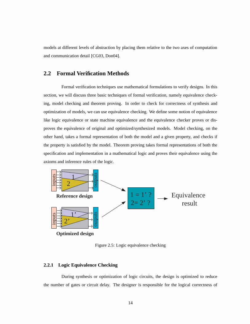
Formal verification techniques use mathematical formulations to verify designs. In this

section, we will discuss three basic techniques of formal verification, namely equivalence check-

ing, model checking and theorem proving. In order to check for correctness of synthesis and

optimization of models, we can use equivalence checking. Wedefine some notion of equivalence

like logic equivalence or state machine equivalence and theequivalence checker proves or dis-

proves the equivalence of original and optimized/synthesized models. Model checking, on the

other hand, takes a formal representation of both the model and a given property, and checks if

the property is satisfied by the model. Theorem proving takesformal representations of both the

specification and implementation in a mathematical logic and proves their equivalence using the

axioms and inference rules of the logic.

1 = 1’ ? 2= 2’ ?

inpu

ts

outp

uts

1 2

inpu

ts

outp

uts

1’ 2’

Equivalence result

Reference design

Optimized design

Figure 2.5: Logic equivalence checking

2.2.1 Logic Equivalence Checking

During synthesis or optimization of logic circuits, the design is optimized to reduce

the number of gates or circuit delay. The designer is responsible for the logical correctness of

14

any such transformation. A logic equivalence checker checks that the result of the synthesis or

optimization is equivalent to the original design. This is achieved by dividing the model into logic

cones between registers, latches or black-boxes as shown inFigure 2.5. The corresponding logic

cones are then compared between original and optimized models.

Logic cones can be described with boolean expressions and thus represented as boolean

decision diagrams (BDDs) [Bry86] or some normal representation like conjunctive normal form

(CNF). Since BDDs have a canonical form, we can reduce the original and optimized cones to

their respective canonical forms and check if they are idential. This requires an ordering of the

boolean variables in the expression. The size of the BDD is highly sensitive to this ordering.

Alternately, satisfiability solvers can be used to compare the boolean expressions. This technique

is the most popular formal technique in industry and is widely applied at the GATE/RTL level to

ensure correctness of logic synthesis.

2.2.2 FSM Equivalence Checking

Logic equivalence checker checks only the equivalence of the combinational part of

the circuit. There are also techniques to check equivalenceof the sequential part of the design

[SDN87]. In order to understand those techniques, we have todefine the notion of a finite state

machine. A finite state machine (FSM) is a tuple consisting ofa set of inputs, a set of outputs and a

set of states. Some of the states are designated as initial states and some as final states. Transitions

between states are defined as a function of current state and the input. An output is also associated

with every state. Formally, we can write

M =< Q ,I ,O,S ,F ,δ,σ >, where

Q = set of all states

I = set of all inputs

O = set of all outputs

S ⊂ Q = set of initial states

F ⊂ Q = set of final states

δ ⊂ Q × I ×Q = transition function

σ ⊂ Q ×O = output labeling of each state.

15

We can think of a FSM as a language acceptor. Assume that we start from an initial state

and supply input symbols from a string S, with each input causing a state transition. If we reach a

final state once all the inputs from S are exhausted, then S is said to be accepted by the FSM. The

set of all acceptable strings forms the language of the FSM. We also define the notion of a product

FSM. The product of two finite state machinesM1 andM2 has the same behavior as ifM1 andM2

were running in parallel. Formally, given

M1 = (Q1,I1,O1,S1,F1,δ1,σ1)

M1 = (Q2,I2,O2,S2,F2,δ2,σ2)

The product state machineM = M1×M2 is defined as

M = (Q ,I ,O,S ,F ,δ,σ), where

Q = Q1×Q2

I = I1× I2

O = O1×O2

S = S1×S2

F = F1×F2

The transition function is defined as follows. If there is a transition from stateq1 to q′1 for input

i1 in M1 and there is a transition from stateq2 to q′2 for input i2 in M2, then there is a transition

from (q1,q2) to (q′1,q′2) for input i1, i2 in M1×M2. The output labeling ofM1×M2 is defined as

follows. If (q1,o1) ∈ σ1 and(q2,o2) ∈ σ2, then((q1,q2),(o1,o2)) ∈ σ.

We can now define equivalence of FSM models by using the previously discussed no-

tions and concepts. The specification and its implementation are both represented as FSMsMs and

Mi respectively. It must be ensured that the input and output alphabet of the two machines should

be the same.

We derive the product machineMs×Mi using cross product of FSMs. Now all the states

in Ms×Mi that have pair of differing outputs are labeled as final states. In Figure 2.6, the states

ps, pt andqr have output pairs with non-identical symbols (xy or yx) and are thus labeled as final

states. We also keep only those transitions that have the same symbols in the input pair. What

we are trying to prove is that for the same sequence of inputs,Ms and Mi would produce the

16

p

q

x

y

a

b

r

s

x

y a

b

t y

b

pr

qr

ps pt

qs qt

xx

yx

xy xy

yy

yy

aa

bb

bb

× = p

q

x

y

a

b

r

s

x

y a

b

t y

b

pr

qr

ps pt

qs qt

xx

yx

xy xy

yy

yy

aa

bb

bb

× =

M s M i M s M i X

Figure 2.6: FSM equivalence checking

same sequence of outputs. In other words, any state with a pair of non-identical outputs should

never be reached. Since such states are the final states in theproduct FSM, they should never

be reached. Therefore the product FSM should not accept any language. This notion is called

language emptiness. Showing language emptiness means starting from the set of initial states in

Ms×Mi and performing a reachability analysis. If any of the final states is reachable, then the

specification and implementation are not equivalent.

True / False + counter - example Model

Checker

P = P2 always leads to P4 s1

s4 s3

s2 P1

P3 P4

P2

M

P = P2 always leads to P4 s1

s4 s3

s2 P1

P3 P4

P2

M

Figure 2.7: Model checking of a transition system

2.2.3 Model Checking

Model checking [CGP00] is a formal technique for property verification illustrated in

Figure 2.7. The model is represented as a state transition system (also called a Kripke structure),

which consists of a finite set of states, transitions betweenstates and labels on each state. The state

labels are atomic properties that hold true in that state. The model checking problem is simply

defined as a verification that a temporal property P is satisfied by the model defined as a state

17

transition system (M,s), where s is the start state for the model execution. We write the model

checking problem asM,s |= P. For example, in the model of a D-flip flop the state variables

would be the input, the clock, the output, its complement, and the reset. The states would be all

possible values of the state variables. A simple property might be that if the reset signal is 0, then

eventually the output will be 0. In figure 2.7 we loosely defineP as “if P2 is satisfied, then P4

will always be satisfied”. The model checker needs to get suchproperties in a formal input format.

Temporal logics [Pnu77] are such formalisms that may be usedfor specifying temporal properties.

s1

s2 s4

s4 s4 s3

s4 s4 s4 s2

Figure 2.8: Example of a computation tree

The most common temporal logic is the computation tree logic(CTL*). Formulas of

CTL* describe properties on computation trees. These treesare formed by taking a start state of

the transition system as root and unrolling all reachable paths from that state. Temporal properties

can by graphically visualized on this computation tree. Figure 2.8 shows the computation tree

rooted atS1 for the transition system in Figure 2.7. CTL* formulas consist of atomic properties,

temporal operators and path quantifiers. Temporal operators include

• Next state operator X, where X(P) means that P will hold in thesecond state,

• Eventual operator F, where F(P) means that P will hold some time in the future,

• Always operator G, where G(P) means that G will hold all the time,

• Until operator U, where U(P1, P2) means that P1 will hold until P2 becomes true, but may

not afterwards

18

• Release operator R, where R(P1, P2) means that P1 will start holding true from the last state

that P2 was true

Besides the temporal operators, we define path quantifies on the computation tree. Quantifier A(P)

implies that P will hold true on all paths on the tree and quantifier E(P) implies that P will hold true

for at least one path of computation tree. Using these operators and quantifiers, we can express

our original property “if P2 holds then P4 will always hold” from figure 2.7. Since P2 only holds

in states2, we can pose this model checking problem as

M,s2 |= A(F(P4))

The model checker works on the state transition system of themodel and the given

property and produces a result TRUE is the property holds in the model. If the property does not

hold, the checker gives a counter-example to show that the property is violated. This feature of

model checking is very helpful in debugging because it provides a readymade test case.

The major problem with model checking is the state space explosion problem. The state

transition system grows exponentially with the number of state variables. Therefore, memory

for storing the state transition system becomes insufficient as the design size grows. Symbolic

model checking [JEK+90] avoids creation of explicit graph data structures for representing state

transition systems. Instead, the atomic properties and state transitions are expressed as a boolean

expression of the state variables in the model. This alleviates the problem of too many states to a

large extent.

2.2.4 Theorem Proving

In general, theorem proving [CRSS94, M.J88] is a technique where a model is specified

in a formalism. The formalism provides for objects and composition rules to create models and a

set of axioms and inference rules to apply transformations on a given model. Logic equivalence

checking may be considered a special case of theorem proving, where the underlying formalism

is boolean algebra.

Due to its generality and mathematical basis, theorem proving can be applied to almost

any verification problem in any domain. In the domain of circuits and systems, higher order logic

19

is used to prove properties on models. The theorem proving problem may be posed as follows.

Given two expressions in some logic, derive a proof using therules of that logic and the problem

domain for the expressions’ equivalence or otherwise.

The proof uses certain assumptions about the problem domainand axioms of the math-

ematical logic. In the domain of circuit design, an assumption might be that power supply is

always at logic level 1 while ground is logic 0. The proof is constructed by breaking down a com-

plex proof goal into smaller goals. The smaller goals are then simplified using assumptions and

then passed onto automatic theorem prover. Theorem provingis still a largely manual process.

Several steps of manually simplifying and breaking down proof goals may be required before an

automatic prover can solve it.

Vdd

Gnd

x y

w1

w2

Figure 2.9: A CMOS inverter implementingy = ¬x

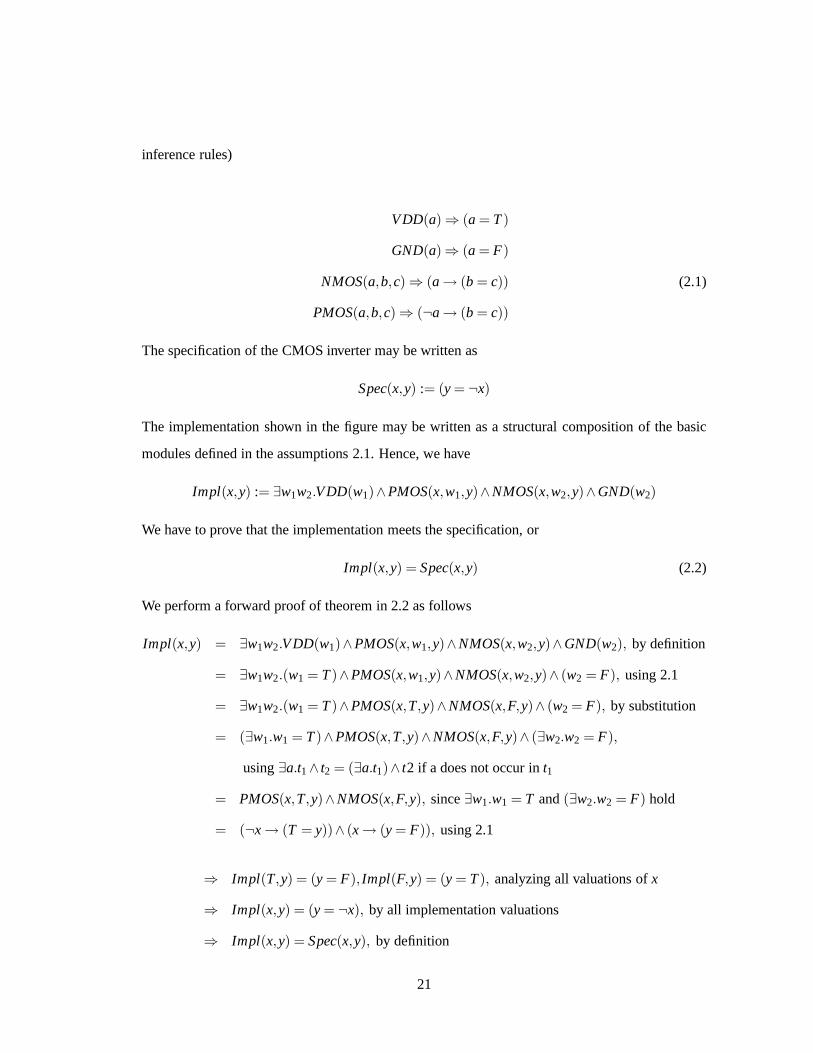
We present a simple example of the use of theorem proving for verifying circuits due

to Gordon [Gor88]. Suppose we have to prove that the CMOS inverter circuit, shown in Figure

2.9, inverts the input logic. We start with the basic assumptions about voltage levels and logic

levels and the behavior of P and N transistors. The formula for the implementation is derived by

conjunction of the various components of the inverter. The specification formula simply states

that the output is logical inverse of input. The proof process takes the implementation formula

and reduces it to the specification formula by a number of steps. Each proof step uses either an

inference rule, an axiom or an already proven theorem.

For the CMOS inverter in Figure 2.9, letw1 be the net connected to power supply (VDD).

Let w2 be the net connected to ground (GND). Let x be the input andy the output variable.

Using the assumptions about PMOS and NMOS transistors, we get the following assumptions (or

20

inference rules)

VDD(a) ⇒ (a = T)

GND(a)⇒ (a = F)

NMOS(a,b,c) ⇒ (a→ (b = c)) (2.1)

PMOS(a,b,c) ⇒ (¬a→ (b = c))

The specification of the CMOS inverter may be written as

Spec(x,y) := (y = ¬x)

The implementation shown in the figure may be written as a structural composition of the basic

modules defined in the assumptions 2.1. Hence, we have

Impl(x,y) := ∃w1w2.VDD(w1)∧PMOS(x,w1,y)∧NMOS(x,w2,y)∧GND(w2)

We have to prove that the implementation meets the specification, or

Impl(x,y) = Spec(x,y) (2.2)

We perform a forward proof of theorem in 2.2 as follows

Impl(x,y) = ∃w1w2.VDD(w1)∧PMOS(x,w1,y)∧NMOS(x,w2,y)∧GND(w2), by definition

= ∃w1w2.(w1 = T)∧PMOS(x,w1,y)∧NMOS(x,w2,y)∧ (w2 = F), using 2.1

= ∃w1w2.(w1 = T)∧PMOS(x,T,y)∧NMOS(x,F,y)∧ (w2 = F), by substitution

= (∃w1.w1 = T)∧PMOS(x,T,y)∧NMOS(x,F,y)∧ (∃w2.w2 = F),

using∃a.t1∧ t2 = (∃a.t1)∧ t2 if a does not occur int1

= PMOS(x,T,y)∧NMOS(x,F,y), since∃w1.w1 = T and(∃w2.w2 = F) hold

= (¬x→ (T = y))∧ (x→ (y = F)), using 2.1

⇒ Impl(T,y) = (y = F), Impl(F,y) = (y = T), analyzing all valuations ofx

⇒ Impl(x,y) = (y = ¬x), by all implementation valuations

⇒ Impl(x,y) = Spec(x,y), by definition

21

2.2.5 Drawbacks of Formal Verification

Formal verification methods have not been as well accepted inthe industry as simulation

based methods because of several drawbacks. Logical equivalence checking works only for com-

binational logic and FSM equivalence checking requires both specification and implementation

machines to have the same set of inputs and outputs. Model checking, besides suffering from the

state explosion problem, is not suitable for all types of designs. Since it needs a state transition

system, it works best for control intensive designs like protocol compliance etc. Automatic theo-

rem proving has not become very popular in the industry because of several reasons. The foremost

reason is the amount of manual intervention required in running the theorem prover. Since dif-

ferent applications have different kinds of assumptions and proof strategies, it is infeasible for a

theorem proving tool to generate the entire proof automatically. Secondly, most designers lack a

background in mathematical logic. Therefore, it requires ahuge investment and long training time

for them to start using theorem proving efficiently.

2.2.6 Improvements to Formal Verification Methods

There have been several improvements to formal techniques,particularly in model check-

ing. Symbolic model checking encodes the state transition system using BDDs, which is much

more compact than exhaustively enumerating the states and transitions. Bounded model check-

ing [CKY03, KCY03] is a variant of model checking that checksif a model satisfies a property

on paths of length at most K. The number K is incremented untila bug is found or the problem

becomes intractable. Also, for bounded model checking, theentire kripke structure of the model

need not be created, which alleviates the problem of state explosion.

Partial order reduction techniques [ABH+97] are usually used in model checking of

asynchronous systems, where concurrent tasks are interleaved rather than being executed simul-

taneously. It uses the commutativity of concurrently executed transitions, which result in the

same state when executed in different orders. Abstraction techniques [CGL94] are used to create

smaller state transition graphs. The specified property is described using some state variables.

The variables that do not influence the specified property areeliminated from the model, thereby

preserving the property while reducing the model size.

22

2.2.7 Semi-Formal Methods: Symbolic Simulation

The idea behind symbolic simulation is to significantly minimize the number of simu-

lation test vectors, for the same coverage, by using symbolsinstead of explicit test vectors. In

symbolic simulation [Bry90], the stimulus applies booleanvariables as inputs to the simulation

model. During simulation, the internal variables and outputs are computed as booelan expressions

of the input variables. In order to check for correctness, the output expression is compared with

the expected output expression for logic equivalence. BDDscan be used to store the boolean ex-

pressions. Since, BDDs of equivalent boolean expressions can be reduced to the same canonical

form, the equivalence of specified output expression to simulated output expression can easily be

checked. However, as the logic depth increases, the size of the BDDs increases exponentially.

Therefore, for larger circuits, where the BDD size may blow up, SAT solvers [MMZ+01] may be

used.

2.3 Evaluation Metrics for Verification Techniques

In order to determine the most suitable verification method,one can define some metrics

to evaluate them. The three most common metrics that we discuss here are coverage, cost and

scalability. Coverage of a verification method determines how much of the design functionality

has been tested. Cost includes the money spent on purchase oftools, hiring of experts and the

training of users. Scalability of the technique shows if there are any limitations on the size or type

of design that we are verifying.

Formal verification claims to provide complete coverage. However, the coverage is lim-

ited to the given property and the richness of the formalism that is used for model representation.

For instance, model checking covers all possible states in the state transition representation of

the model for a given property. Logic equivalence checking covers the combinational part of the

model only. Nevertheless, the coverage of formal methods, if they are applicable, is significantly

more than that of simulation based methods for the same run-time. Using assertions in the design

can help make better test cases that exercise the assertions, thereby ensuring that the tests are use-

ful and valid. Pseudo random testing, on the other hand, would generate a lot of test inputs that

are invalid for the design, and hence wasted.

23

Cost and effort of a verification method influences the designphase in which it is used.

For instance, the preliminary phase usually employs simulation to uncover most of the easy bugs.

This is because most designers have experience with simulation tools and debuggers and it is thus

cost effective. It is counter intuitive to employ expensivetools and expert verification engineers

during early bug hunting. As the verification process continues and the design models stabilize,

bugs become harder to find. In the latter phase, specialized and more expensive techniques like

model checking or theorem proving may be used. Assertions are also used to generate more

directed tests and to verify correctness on corner cases. The universal 80-20 rule applies to most

design verification cases, that is, 20% of the total cost uncover 80% of the bugs and vice versa.

The performance of a verification method on different sizes and abstraction levels of

models determines its scalability. Some methods like logicequivalence checking are limited to

RTL models or below. Similarly, model checking is constrained by the number of state variables

in the model. Compared to other techniques, simulation scales very well for alltypes of models.

Almost any executable model at any level of abstraction can be simulated.

If we look at the trend in the acceptance of verification techniques in the industry, we

find that methods with a severe drawback have been generally avoided. Model checking suffers

from poor scalability and theorem proving is way too expensive, thereby making equivalence

checking the most commonly used technique in the industry. Similarly, assertion based techniques

may require extra cost but they are replacing pseudo random simulation because of their better

coverage. Universal adoption of new verification and assertion languages is testimony to this fact.

2.4 Future of System Verification

The new challenges to verification of systems comes from the growth in size and com-

plexity of designs. Individually verified components do notwork together due to interface issues.

Also the sheer size of designs makes modeling and verification too expensive and time consuming.

To answer this challenge, we look towards a disciplined system design methodology. To

design complex systems on chip, the level of model abstraction has been raised. If the semantics

of system level models is well defined, then they can be formalized. Consequently, we can de-

fine transformations from models at one abstraction level toanother. The transformations can be

24

proven to produce equivalence models. Thus, the traditional methods can still be used at higher

levels of abstraction while correct transformations will over, time remove, the need to verify lower

level models for functionality.

2.5 Chapter Summary

In this chapter, we provided an overview of various verification strategies being em-

ployed in the industry today. We showed how coverage of traditional simulation is improved

by using directed test vectors instead of random vectors. Better monitoring techniques such as

graphical views of simulation results aid in understandingand debugging of designs. Emulation

techniques provide “at-speed” simulation of the design by actually prototyping it in hardware. We

also looked at formal verification methods that are slowly, yet surely, making inroads into the veri-

fication market. We presented the theoretical aspects of formal methods such as logic equivalence

checking, model checking, theorem proving and symbolic simulation.

In conclusion, we found that as the size and complexity of system designs increase,

traditional techniques might not be able to keep pace. A system design methodology will well

defined model semantics may be a possible solution to the problem. Specifying the design at a

higher level of abstraction would make traditional verification and debugging tractable because

of smaller model size. Well defined model semantics would make it possible to define and prove

correct transformations for automatic model refinement. Therefore, formalisms for representing

and correctly transforming models would make complete system verification much faster.

25

Chapter 3

Model Algebra

A modeling formalism may be defined as a set of objects and composition rules that

represent relationships between the objects. Our goal is tohave a formalism that can allow the

designer to express executable system models at different levels of abstraction. For instance,

one should be able to express a model that shows only the functionality of the system using the

objects and composition rules of the formalism. Also, one should be able to express models with

structural details, using the same objects and compositionrules. Given a model and its abstraction

level, one should be able to identify the various structuralartifacts within the model. Finally, a

model expressed in such a formalism, should be executable sothat it may be used to evaluate the

design. The formalism must, therefore, have clear execution semantics.

3.1 Definition

A system can be viewed as a block of computation; with inputs and outputs for stimuli

and response, respectively. This computation block is composed of smaller computation blocks

that execute in a given order and communicate amongst themselves. Thus, for modeling pur-

poses, it is imperative to have primitives for computation and communication. We will refer to

the computation units as behaviors. A behavior has ports that allow it to be connected to other

behaviors. The units of communication are variables and channels. These communication objects

have different semantics. Variables allow a “read, computeand store” style of communication,

while channels support a synchronized double handshake style of communication. Composition

26

rules are used to create an execution order of behaviors and to bind their ports to either variables

or channels. A system is thus represented as a hierarchical behavior composed of sub-behaviors

communicating via variables and channels.

3.1.1 Objects

The objects of MA can be defined as the tuple

, where

B is the set of behaviors

C is the set of channels

V is the set of variables

I is the behavior interface

P is the set of behavior ports

A is the set of address labels

We also define a subsetB I of B representing the set of identity behaviors. Identity

behaviors are those behaviors that, upon execution, produce an output that is identical to their

input. In general, we will use the convention of naming identity behaviors ase followed by a

subscript. Each of the variables inV hastypeassociated with it. We defineQ to be the subset of

V such that all variables inQ are of typeboolean.

3.1.1.1 Ports

Each behavior has an associated object called its interface. The interface carries the

ports of the behavior that are represented by their association to the behavior. Hence, to internal

behaviors of a hierarchical behavior, the port is seen asI , wherep∈ P . The port is treated

like any other local variable except that we restrict operations on it, depending on itsdirection.

Local behaviors can either write to a port, in which case it isknown as theout-port, or they may

read from the port, in which case it is called thein-port. If both read and write are allowed, th port

is calledinout-port. When the same portp is accessed from outside of behaviorb, it is written as

b .

27

3.1.1.2 Addressing

Behaviors communicate with each other using either memory or channels. Essentially,

memory based communication follows the SW programming paradigm, where one behavior writes

data into a variable through an out-port and another behavior reads it via an in-port. Behaviors ex-

ecuting concurrently use synchronized data transactions amongst themselves for communication.

Channels serve as the media for such transactions. Each transaction uses an address to identify

the sender and the receiver behaviors. The transactions can, thus, be visualized to take place over

virtual links, that are labeled by distinct addresses. Eachof the links is associated with a channel.

Hence, such a link may be written asc < a >, where the link uses channelc and has the address

a. Two transactions on a channel cannot share a link if they might take place simultaneously. In

other words, all transactions on a single link must be totally ordered in time.

3.1.2 Composition Rules

Composition rules on the objects in MA are defined as relations in MA. These relations

may contain two or more objects. Each composition rule creates a term, which may be further

composed, in a particular format, to create hierarchical behaviors.

3.1.2.1 Control flow

A control flow composition (Rc)determines the execution order of behaviors during

model simulation. We write the relation as

q : b1&b2& ...&bn b

where∀i,1≤ i ≤ nb,bi ∈ B ∪ I ,q∈ Q . The composition rule implies thatb executes afterall the

behaviorsb1 throughbn, called predecessors in the relation, have completedand q evaluates to

TRUE. Rc is said tolead to bunder the conditionq. It implies a synchronization whereb must

wait for all predecessors to complete. The degenerate case of the control flow relation is of the

form q1 : b1 b. Here, we only have a single predecessor, sob may start executing afterb1 if q1

evaluates to TRUE, even if there are other control flow relations leading tob. A relation with a

TRUE condition, eg. 1 :b1 b2 will be shorthanded asb1 b2.

28

3.1.2.2 Non-blocking write

This composition rule (Rnw) is used to indicate that a behavior uses its out-port to write

to a variable or an out-port of its parent behavior. In the case of a write to a data variable, we use

the expression

b → v

whereb is the out-port of the writing behavior andv indicates the memory into which

the data is written. In its other manifestation, this composition rule can be used to create a port

connection, written as

b → I < p′ >

In this case, the composition rule indicates a port-map in a hierarchical behavior. Note that< p′ >

must also be an out-port or inout-port.

3.1.2.3 Non-blocking read

This composition rule (Rnr) is used to indicate that a behavior uses its in-port to read

data from a variable or through an in-port of its parent behavior. In the case of a read from a data

variable, we use the expression

v→ b 

whereb is the in-port of the reading behavior andv indicates the memory from which

the data is read. In its other manifestation, this composition rule can be used to create a port

connection, written as

I < p′ >→ b 

In this case, the composition rule indicates a port-map in a hierarchical behavior. Note that< p′ >

must also be an in-port or inout-port.

3.1.2.4 Channel transaction

This composition rule (Rt ) indicates a data transfer link from the sender behavior to one

or more receiver behavior(s) over a channel. The semantics of the composition rule ensure that

the sender and the receiver(s) are ready at the time of the transaction. In other words, it follows a

29

rendezvous communication mechanism. The sender and receiver ports as well as the logical link

of the channel are also indicated in the relation. We write this relation as

c < a >: b 7→ b1 < p1 > &b2 < p2 > ...&bn < pn >

whereb is the out-port of the sending behavior andb1 < p1 > throughbn < pn > are the

in-ports of the receiving behaviors. The transaction takesplace over channelc and uses the link

addresseda.

3.1.2.5 Blocking write

This composition rule (Rbw) is used to indicate the port connection for the sender part

of a transaction. The sender behavior writes to the out-portof its parent behavior through one of

its own out-ports. Eventually, the port will be bound to a channel transaction. Thus, the blocking

write relation facilitates the creation of hierarchy in themodel. We represent a blocking write by

the expression

< a >: b 7→ I < p′ >

whereb is the out-port of the writing behavior. The portI < p′ > on the parent behavior

of b will eventually be bound to another blocking write relationor a channel transaction relation

with addressa.

3.1.2.6 Blocking read

This composition rule (Rbr) is used to indicate the port connection for the receiver part

of a transaction link. The receiving behavior(s) read(s) from the in-port of their parent behavior

through one of their own in-ports. Eventually, the port of the parent behavior will be bound to

a channel transaction. Thus, the blocking read relation facilitates the creation of hierarchy in the

model. We represent a blocking read by the expression

< a >: I < p′ > 7→ b1 < p1 > &b2 < p2 > ...&bn < pn >

whereb1 < p1 > throughbn < pn > are the in-port(s) of the receiving behavior(s). The port

I < p′ > will eventually be bound to another blocking read relation or a channel transaction

relation. The address of the virtual link (< a >) will be used for binding this port.

30

3.1.2.7 Grouping

This composition rule (Rg)is used to indicate a collection oftermsformed using above

composition rules. Essentially, grouping is used to createhierarchy of behaviors, by collecting the

various compositions of sub-behaviors, local channels andlocal variables. This commutative and

associative relation is written as

r1.r2....rn

where∀i,1≤ i ≤ n, r i ∈S

{Rc,Rnw,Rnr,Rt ,Rbw,Rbr,Rg}.

Essentially, a grouping of model algebraic terms is another(more complex) term. Nor-

mal set theoretic operations like union and substraction may be performed to manipulate complex

terms formed by grouping. For example, we can use the dot (“.”) operation to add another term to

a group as follows

(r1.r2....rn).rn+1 = r1.r2....rn.rn+1

Similarly, we may substract a term from a group as follows

(r1.r2....rn)− r i = r1.r2....r i−1.r i+1...rn

Finally, we also define abelongs-torelation between sub-terms of a complex term and the complex

term itself as follows

∀i, such that 1≤ i ≤ n, r i ∈ r1.r2...rn

3.2 Model Construction with MA

So far, we have seen the various objects and composition rules of MA. In this section, we

look at how to construct hierarchical system models in MA using these objects and composition

rules.

3.2.1 Hierarchy

Using the control flow relations, we can compose behaviors such that they execute in a

desirable order. Most SLDLs provide for hierarchical compositions of behaviors to aid modeling.

31

Virtual Starting Point

Virtual Terminating Point

b

b 1 b 2

b vsp

b vtp

q1

q2

Figure 3.1: Control flow within hierarchical behaviors

In MA, hierarchy is achieved using the interface object and its relation to behaviors. In figure 3.1,

a behaviorb (shown as rounded rectangle) is created by hierarchical composition of sub-behaviors

b1 andb2. Note thevirtual starting point(VSP) and thevirtual terminating point(VTP) behaviors

of b. The VSP is the identity behaviorvspb that is the first to execute insideb. Other sub-behaviors

of b are executed aftervspb, depending on outgoing control relations (shown using broken arcs

and circular nodes labeled with control conditions) fromvspb. We can see in figure 3.1 that the

VSP in this casevspb is triggering the execution of sub-behaviorb1. Due to its nature, a VSP

behavior would only have outgoing control to other sub-behaviors of b. Likewise, the identity

behaviorvt pb is the last behavior to execute insideb, and will only have incoming control from

other sub-behaviors ofb. All hierarchical behaviors are assumed to have a unique VSPand a VTP.

Hence, the starting and terminating control relations ofb can be written as

vspb b1.b2 vt pb

3.2.2 Parallel and Conditional Execution

Most SLDLs provide for special constructs to create different types of behavioral hier-

archies. The common ones are parallel composition and conditional composition. Figure 3.2(a)

shows a parallel composition of behaviorsb1 andb2. A typical SLDL may allow construction of

a parallel composition using a statement like

par {run b1; run b2}.

Let the resulting behavior be calledbpar. The execution ofbpar indicates that bothb1 andb2 are

32

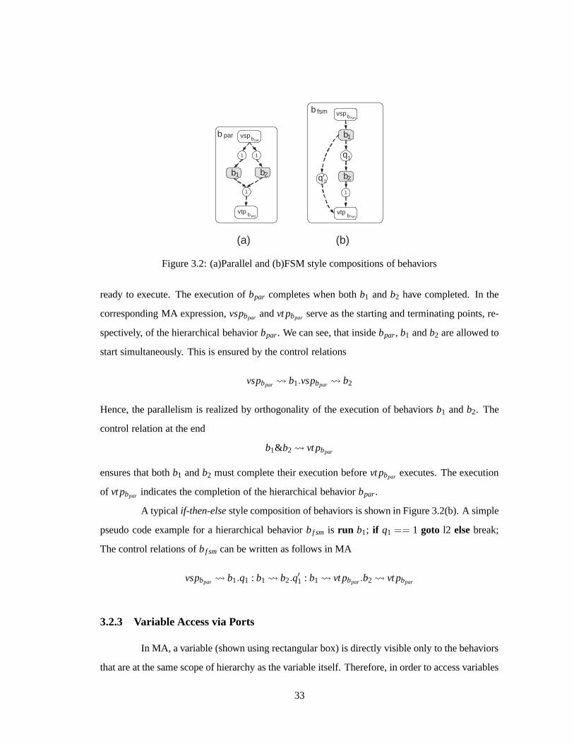
b 1 b 2

b 1

b 2

(a) (b)

par b

fsm b

q 1

b vsp par

b vtp par

b vsp fsm

b vtp

fsm

1

1 1

1

q' 1

Figure 3.2: (a)Parallel and (b)FSM style compositions of behaviors

ready to execute. The execution ofbpar completes when bothb1 andb2 have completed. In the

corresponding MA expression,vspbpar andvt pbpar serve as the starting and terminating points, re-

spectively, of the hierarchical behaviorbpar. We can see, that insidebpar, b1 andb2 are allowed to

start simultaneously. This is ensured by the control relations

vspbpar b1.vspbpar b2

Hence, the parallelism is realized by orthogonality of the execution of behaviorsb1 andb2. The

control relation at the end

b1&b2 vt pbpar

ensures that bothb1 andb2 must complete their execution beforevt pbpar executes. The execution

of vt pbpar indicates the completion of the hierarchical behaviorbpar.

A typical if-then-elsestyle composition of behaviors is shown in Figure 3.2(b). A simple

pseudo code example for a hierarchical behaviorbf sm is run b1; if q1 == 1 goto l2 elsebreak;

The control relations ofbf sm can be written as follows in MA

vspbpar b1.q1 : b1 b2.q′1 : b1 vt pbpar.b2 vt pbpar

3.2.3 Variable Access via Ports

In MA, a variable (shown using rectangular box) is directly visible only to the behaviors

that are at the same scope of hierarchy as the variable itself. Therefore, in order to access variables

33

b b 1

b 2

v2

v1 hier b

in

out

p1

p2

Figure 3.3: Using ports for non-blocking data flow in hierarchical behaviors

at higher levels of hierarchy, data ports are used. Ports arevisualized as tiny boxes on the behavior

interfaces. As shown in Figure 3.3, behaviorb1 reads variablev1 present inbhier via the port

“in” of its parent b. Hence, to realized this port connection, we need terms at different levels of

behavior hierarchy. At the scope ofbhier, we use the non-blocking relationv1 → b < in >. At the

scope ofb, we use the port connection (shown using solid directed arcs) from the interface ofb to

b1. We can write this as the relation

I < in >→ b1 < p1 >

The dual of read port connection is the write port connectionas shown by the access of

variablev2 from behaviorb2 in figure 3.3. In this case, the port “out” ofb is used to realize the

variable access. The term at the scope ofbhier is

b < out >→ v2

while the term at the scope ofb is

b2 < p2 >→ I < out >

3.2.4 Channel Access via Ports

As in the case of non-blocking reads and write, MA provides mechanism for blocking

reads and writes (shown using solid arcs labeled with link address) via ports. For instance, in

Figure 3.4, we see channel transactions fromb to b′1 andb′2 overc, labeleda1 anda2 respectively.

After zooming into the hierarchy ofb, we see that the transactions are taking place fromb1 to b′1

andb2 to b′2. The portsp1 andp2 of b makes the channelc visible tob1 andb2. Therefore, using

the relation

< a >: b1 < p11 > 7→ I < p1 >

34

b 1

b p11

c

p1 a1

b 2 p22

p2 a2

b' 1

b' 2

a1

a2

p11'

p22'

a1

a2

Figure 3.4: Sharing channel for transactions with different addresses

behaviorb1 can access channelc. However, this requiresp1 to be bound to the transaction link

addressed bya1.

In MA several virtual links may share a single channel. Each of the virtual links are

assigned a different address, but the data transfer takes place on the same medium. Figure 3.4

shows an instance of channel sharing. Here, the two virtual links with addresses< a1 > and

< a2 > use a common channelc. Transactions may be attempted concurrently on these links.

However, due to sharing of the channel, we can allow only one transaction at a time. Thus, an

arbiter in the channel must ensure that only one transactionmay take place at any time. In MA,

this is guaranteed by the mutual exclusion property of the channel, where the channel is a shared

resource and each transaction is treated as a critical section. This allows us to connect several

different virtual links to the same channel.

3.2.5 Using Identity Behaviors

A class of behaviors in MA is known as the identity behavior. As the name suggests,

these behaviors have the same output as the input. As a resultthey do not have any computation

inside them. They have two ports namely the “in” port for reading the input and an “out” port for

writing the output. In general, the identity behavior first reads data from the “in” port to a local

variable and then writes this variable to the “out” port. Theactual implementation of the read and

write within the identity behavior depends on the port connections.

There are four basic manifestations of the identity behavior as shown in figure 3.5. In

the first case, as shown in figure 3.5(a), both the “in” and “out” ports of the identity behaviore1

are connected to variables. Hence, the respective read and write are non-blocking relations. In

35

(a) (b)

(c) (d)

e 4 out

c

a in

c' a'

e 3 out

c a

v

in

e 1 out

v

in

v'

e 2 out

c a

v in

b a

b a

p

p

b

a

p

b' a'

p'

Figure 3.5: Various manifestations of the identity behavior

MA, the read/write relations ofe1 are expressed as

v→ e1 < in > .e1 < out >→ v′

The second case of identity behavior is shown in figure 3.5(b). Here, the “in” port is

connected to a variable, hence the input is read using a non-blocking relation. On the other hand,

the “out” port is connected to channelc. Hence, the output needs to be sent tob using a blocking

write relation. In MA, the read/write relations ofe2 are expressed as

v→ e2 < in > .c < a >: e1 < out > 7→ b 

The third case of identity behavior is shown in figure 3.5(c).Here, the “in” port is

connected to a channelc, hence the input is read from behaviorb using a channel transaction. On

the other hand, the “out” port is connected to variablev. Hence, the output needs to be written

using a non-blocking write relation.In MA, the read/write relations ofe3 are expressed as

c < a >: b 7→ e3 < in > .e3 < out >→ v

Finally, the fourth manifestation of identity behavior is shown in figure 3.5(d). Here, the

“in” port of e4 is connected to a channelc for reading data fromb. Hence the input is read using

36

a channel transaction relation. The “out” port ofe4 is also connected to a channel namedc′ for

writing data tob′. Hence, the output is also written using a channel transaction relation. In MA,

the read/write relations ofe4 are expressed as

c < a >: b 7→ e4 < in > .c′ < a′ >: e4 < out > 7→ b′ < p′ >

3.2.6 Hierarchical Modeling in MA

The model of a system is simply a behavior in MA. Typically, itis a hierarchical behavior

showing the various components and connections of the system and the functionality within these

components.

b1

b2

a

v

p1 p11

p12

p21 p22

p2

b hier b

hier vsp

b hier

vtp

1

q1'

q1

1

Figure 3.6: A hierarchical behavior with local objects and relations

3.2.6.1 Internal and Interface Terms

In MA, it is possible to represent a hierarchical behavior asa grouping of terms involving

its sub-behaviors, its interface and its local variables and channels. Figure 3.6 shows a hierarchical

behaviorbhier. The expression for the hierarchical behavior is written using the local objects and

their compositions. For instance, in the given behaviorbhier, we can see sub-behaviorsb1 andb2.

We can also see control flow relations that determine the execution scenario under the conditions

labeled on the control arcs. We also see data flow relations, both amongst sub-behaviors and

between sub-behaviors and the interface. The grouping of relations between local objects will be

referred to as theinternal termsof a hierarchical behavior. Similarly, the grouping of relations

37

involving the interface will be referred to as theinterface termsof the hierarchical behavior.

We can write the hierarchical behavior as a grouping of all its internal and interface

terms, along with the internal terms of its sub-behaviors. The grouping of internal terms for a

given behaviorb is represented as[b]. Thus, we can write

[bhier] = [vspbhier ].[b1].[b2].[vt pbhier ].vspbhier b1.q1 : b1 b2.

q′1 : b1 vt pbhier.b2 vt pbhier.b1 < p12 >→ v.v→ b2 < p21 >

The interface terms ofbhier are represented by|bhier|. From figure 3.6, we can see that

|bhier| =< a >: I < p1 > 7→ b1 < p11 > .b2 < p22 >→ I < p2 >

Finally, we write the hierarchical behavior as a grouping ofits internal and interface

terms. We will use the convention of enclosing the expression for a hierarchical behavior in

braces. Therefore, we get

bhier = ([bhier].|bhier|)

par b b

vsp par

b vtp

par

a

p1 p2 b hier

p

c b3 a

p31

par b b vsp par

b vtp

par p

c

b3

a

p31

(a)

(b)

1

1

1

b1

b2

a

v

p11

p12

p21 p22

b hier b hier

vsp

b hier vtp

1

q1'

q1

1

1

1

1

p1

a

p2

Figure 3.7: Hierarchical behaviorbpar showing (a) local scope, and (b) all scopes down to leaf

behaviors

38

3.2.6.2 Multiple Levels of Hierarchy

In the above example, a conditional hierarchical composition was created. The resulting

behaviorbhier can be used further to create more hierarchical behaviors. For instance, in Fig-

ure 3.7(a), we see behaviorbhier in a parallel composition with behaviorb3. The two behaviors

exchange data using the virtual link addresseda, over channelc. The hierarchical composition

results in a new behavior calledbpar. The expression forbpar is written in MA as follows

bpar = ([vspbpar ].[bhier].b3.[vt pbpar].vspbpar bhier.vspbpar b3.bhier&b3 vt pbpar.

c < a >: b3 < p31 > 7→ bhier < p1 > .bhier < p2 >→ I )

The model of the system can be expressed in Model Algebra using a set of equations (as above)

where each hierarchical behavior is expressed as a groupingof its local behaviors and control and

data depenency terms.

3.3 Execution Semantics

In order to define the execution semantics of MA, the control relations in the model

are captured using theBehavior control graph(BCG). BCG is simply a graph representation of

the control flow in the model. Control dependencies implied by the rendezvous transactions on

channels are also converted into BCG arcs to derive an execution model of the system. In this

section we will first look at the formal execution semantics of model algebra using the BCG.

Then we will look at semantics of channel transactions and how the control dependencies of such

transaction links can be translated to BCG form.

3.3.1 Behavior Control Graph

The BCG is similar in principle to the Kahn Process Network [Kah74], but with some

remarkable differences.It is a directed graph BCG(N,E) with two types of nodes, namelybehavior

nodes(NB) andcontrol nodes(NQ). The behavior nodes, as the name suggests, indicate behavior

execution, while the control nodes represent evaluation ofcontrol conditions that lead to further

behavior executions. Directed edges are allowed from behavior nodes to control nodes and vice

39

q1

qm

q1'

qn'

b1_queue b 1 _ q 1 ' _ q u e u e

b 1 _ q n ' _ q u e u e

b 1

b k

b k _ q n _ q u e u e

Figure 3.8: The firing semantics of BCG nodes

versa. Also, a control node can have one, and only one, out going edge. Thus,

E(BCG)⊂ NB(BCG)×NQ(BCG)∪NQ(BCG)×NB(BCG)

There is a one to one correlation between the BCG and the control relations of the MA

representation. A relation of the form

q : b1&b2& ...&bn b

translates to a BCG with a control node (q), n+1 behavior nodes (b,b1, ...,bn) andn+1 directed

arcs ((b1,q), ...,(bn,q),(q,b)).

The execution of a behavior node, and similarly, the evaluation in a control node, will

be referred to as afiring. Node firings are facilitated by tokens that circulate in thequeues of the

BCG as shown in Figure 3.8. Each behavior node (shown by rounded edged box) in the BCG has

one queue, for instanceb1 queuefor behavior nodeb1. All incoming edges to a behavior node

represent the various writers to the behavior’s queue. The control node (shown by circular node),

on the other hand, has as many queues as the number of incomingedges. Note that a control

node may have only one outgoing edge. This restriction follows directly from the control flow

composition rule of model algebra. As shown in Figure 3.8qn hask queues, one each for edges

from b1 throughbk.

A behavior node blocks on an empty queue and fires if there is atleast one token in

its queue. Upon firing, one token is dequeued from the node’s queue. After firing, a behavior

40

node first updates all variables that it is writing to. Then, it generates as many tokens as its out-

degree, and each token is written to the corresponding queueof the destination control node in a

non-blocking fashion.

A control node, sequentially checks all its queues and blocks on empty queues. That is

if an incoming edge’s queue is empty, we must wait until the behavior on the other end of the edge

has fired. If the queue is not empty, it dequeues a token from the queue and proceeds to check the

next queue. Once we have dequeued one token from each of the incoming queues, the condition

inside the control node is evaluated. If the result is TRUE, then the control node fires. Upon firing,

the control node enqueues one token to the queue of the destination behavior in a non-blocking

fashion. The process of checking the incoming queues is repeated indefinitely.

3.3.2 Channel Semantics

The channel object allows for rendezvous communication [Hoa85, Mil80] between two

concurrently executing behaviors. As discussed before, a channel transaction implies a control

dependency between parts of the communicating behaviors. Without loss of generality, we can

assume both the sender and the receiver to be identity behaviors. We will follow this assumption

in all future discussions.

c

a a

time

Case A: Writer arrives first

rd

wr

wait

rd

wait wr wait

wait

Atomic Transaction

Case B: Reader arrives first

e wr e rd out in

Figure 3.9: Timing diagram of a transaction on a channel

41

3.3.2.1 Channels with single transaction link

Figure 3.9 shows a transaction taking place over channelc. We can express this transac-

tion MA using the termc < a >: ewr < out > 7→ erd < in >. The timing diagram for this channel

transaction shows two instances of execution. In the first instance, called Case A, the writer

reaches the communication point before the reader. By this we mean that during model execution,

ewr is scheduled to execute beforeerd . However, the rendezvous semantics dictate thatewr must

wait until erd is ready before executing. It may be noted that if there is a control dependency from

ewr to erd , the resulting model would deadlock. Hence,erd must be allowed to start independently

of ewr and vice versa. Onceerd is ready to start the transaction, it notifiesewr. The transaction is

thus initiated byewr, that performs a write on the channel. Subsequently,erd reads the data from

the channel.

In the second execution scenario, called Case B, the reader is scheduled before the writer

is ready. This forceserd to wait until ewr is ready to start executing. The shaded part of the

execution, in the timing diagram, indicates the atomic nature of the transaction. Note that the

channel resources (i.e. its local memory) are occupied onlyduring the actual reading and writing

of the data, not during synchronization.

time

rd(a1) wr(a1)

rd(a2) wr(a2) wait

Wait1

e1

e2

c

a1 a1 e1'

e2' a2 a2

Arrival times

Transaction times

Atomic Transaction

e1 e1'

e2 e2'

Wait2

out

out in

in

Figure 3.10: Multiple competing transactions on a single channel

42

3.3.2.2 Channels with multiple transaction links

As discussed earlier, channel sharing is possible for different virtual links, but the trans-

actions are ordered in time. This mutual exclusivity of transactions can be achieved by the use of

semaphores or arbiters. Thus, the shaded part representingthe actual data read and write over the

local memory of channel is mutually exclusive. Consider theconfiguration shown in figure 3.10.

In this case, two virtual links, addresseda1 anda2, are shared over channelc. These links can be

written as a grouping of the following terms

c < a1 >: e1 < out > 7→ e′1 < in > .c < a2 >: e2 < out > 7→ e′2 < in >

The timing diagram shows the actual arrival schedule of the four communicating identity behaviors

and the resulting communication schedule on the channel. Note that despite the fact thate1 arrives

first, transaction ona2 takes place before that ona1. This is because, the data transfer of transaction

addresseda2 is ready to be performed before that fora1. Thus, the data transfers on the channel are

scheduled on first-ready first-serve basis. Although the transaction ona1 is ready to be performed

whene′1 arrives, it must wait for the durationwait2 since the transaction addresseda2 is in progress.

3.3.3 Control paths and dominators

We will now define some useful control flow relations between behaviors in a model,

based on the model’s BCG. A control path from a behaviorb1 to b2 in modelM is simply a non-

zero length path in the BCG ofM from node representingb1 to node representingb2. If such a

path exists, thenb2 is said to bereachablefrom b1, elseb2 is said to beunreachablefrom b1.

A behaviorb is said todominatecontrol flow from b1 to b2 in a given modelM, if

during execution ofM, b always fires at least oncebetweenany two unique firings ofb1 andb2.

This relation betweenb, b1 andb2 is written as

b⊲ (b1,b2)

It must be noted that the dominator relation does not mean that b must exist in all control paths

from b1 to b2. Figure 3.11 shows BCG of a simple model with four behaviorsb1 throughb4. The

control paths fromb1 to b4 are indicated by thick broken arrows labeled CP1 and CP2. It can be

easily seen thatb2⊲(b1,b4), since any firing ofb4 is always preceded by a firing ofq4 andq4 does

43

b 1

b 2 b 3

b 4

q2 q3

q4

vsp

vtp

q1

q5

CP1 CP2

Figure 3.11: Illustration of control paths

not fire untilb2 has fired. However,b2 does not exist in the control path(b1,q3,b3,q4,b4) (labeled

CP2).

A special case of the dominator relation is as follows. Assume there exist behaviorsb

andb′ in modelM such that during any execution ofM, there is atleast one unique firing ofb

before every unique firing ofb′. We say thatb dominatesb′ and we will write the control relation

betweenb andb′ asb⊲b′. It can be easily seen that

b⊲b′ ⇔ (b⊲ (vsp,b′)∧b⊲ (b′,b′))

The RHS of the above equation indicated thatb must fires once between the firing ofvsp(start

of model execution) and the (first) firing ofb′. Any subsequent firings ofb′ (after its first firing)

should also follow a unique firing ofb, as guaranteed by relationb⊲ (b′,b′). This is equivalent to

b⊲b′ by definition of the dominator relation.

From the above definitions, we can also make the following observations

b1 ⊲b2∧b2⊲b3 ⇒ b2 ⊲ (b1,b3) (3.1)

b1 ⊲b2∧b2⊲b3 ⇒ b1 ⊲b3 (3.2)

44

3.4 Notion of Functional Equivalence

Before we begin to verify models written in MA, we must first establish a formal notion

of equivalence. There are several possible notions of equivalence for process algebras like trace

equivalence [BNP02], bisimulation equivalence [Mil80] and so on. The basic purpose of a formal

equivalence notion is to be able to distinguish different models written in a formalism. An equiv-

alence notion is said to bestrongerif it distinguishes more models. For instance two models may

be trace equivalent, but notbisimulation equivalent. However, all models that are bisimulation

equivalent are also trace equivalent. Therefore, bisimulation is astrongernotion of equivalence

compared to trace equivalence. Conversely, trace equivalence isweakerthan bisimulation. The

strongest possible equivalence isisomorphismwhich indicates a syntactic equality of two models.

An interesting comparison of formal notions of equivalencemay be found in [vGG89]

3.4.1 Value Traces

Our notion of functional equivalence is based on the trace ofvalues that certain interest-

ing variables hold during model execution. We will refer to such variables asobserved variables.

Given a modelM and a set of its observed variables, sayOVM , let InitM be the initial assignment

of all the variables inOVM . Let v∈ OVM . We defineτM(v, InitM) as the set of all possible traces of

values assumed byv, when modelM is executed with initializationInitM .

Figure 3.12 shows a simple model, sayM. We have shown the function inside leaf level

behaviors to demonstrate the trace values. Letx andy be the observed variables, with an initial

assignment of 0 andU (undefined). When modelM is executed,b1 fires aftervsp, setting the

value ofy to 2∗0 = 0. sincex < 2, b2 fires and incrementsx to 1. This is followed by another

firing of b1 and so on. Hence, for the given scenario, we have

OVm = {x,y}

InitM = {0,U}

τM(x, InitM) = {{0,1,2,3}}

τM(y, InitM) = {{U,0,2,4,6}}

The model terminates withx= 3 andy= 6. However, it is possible that model execution

45

vsp

vtp

p1

b1

1

p2= p1*2

p2

p1

b2 p2=

p1+1 p2

X<= 2 x y

X > 2

1

Figure 3.12: Example of a model (M) with unique value trace

may never terminate and the traces are infinitely long.

Figure 3.13 shows a new model, sayM′. In this model, the behaviorsb1 andb2 are

rearranged to execute in parallel. As in the previous case, let x andy be the observed variables,

with an initial assignment of 0 andU (undefined). When modelM′ is executed, eitherb1 or b2

may fire first aftere. Therefore, the value ofy may become 0 ifb1 fires first, or become 2 ifb2

fires first (modifyingx to 1). However, by the timee2 executesx is definitely 1. Sincex < 2, e1

fires again, allowing eitherb1 or b2 to fire first. The process continues untilx becomes 3, Hence,

for the given scenario, we have

OVm = {x,y}

InitM = {0,U}

τM(x, InitM) = {{0,1,2,3}}

τM(y, InitM) = {{U,0,2,4},{{U,0,2,6},{{U,0,4},

{{U,0,4,6},{{U,2,4},{{U,2,6},{{U,2,4,6}}

46

vsp

vtp

p1

b1

1

p2= p1*2

p1 b2

p2= p1+1

p2

X<= 2

x y

X > 2

1

e1

1 1

p2

e2

Figure 3.13: Example of a model (M′) with several possible value traces

3.4.2 Trace based equivalence

Given two modelsM andM′ expressed using model algebra, we wish to determine if

they are equivalent with respect to some well defined notion of equivalence. First, we need to

determine a correlation between the two models based on their respective observed variables.

We choose the observed variables of a model as the set of all variables in a model that are not

written exclusively by identity behaviors. The reasoning is that variables that are connected to

the output ports of identity behaviors are simply a copy of another variable. Informally speaking,

we consider two models to be functionally equivalent, if they have one-to-one correspondence of

observed variables and the trace of values assumed by those variables during model execution is

identical, given the same initial assignment. The traces should be identical for all possible initial

assignments.

More formally, in order to show equivalence ofM andM′, we require that,

|OVM| = |OVM′ |

and there exists a bijective mapping fromOVM to OVM′ . We will represent the mapping of respec-

47

tive elements by the↔ symbol. Therefore, we have

∀v∈ OVM ,∃v′ ∈ OVM′ , such thatv↔ v′

Let InitM be the initial assignment of all variables inOVM andInitM′ be the initial assignment of

all variables inOVM′ . ModelsM andM′ are equivalent if

∀InitM , InitM′ ,∀v∈ OVM,v′ ∈ OVM′ , such thatv↔ v′

if the initial assignment ofv is equal to the initial assignment ofv′, then

τM(v, InitM) = τM′(v′, InitM′)

3.5 Transformation laws of MA

We will now define laws of MA that will allow us to perform useful functionality pre-

serving transformations on a model. For clarity, We will demonstrate these transformations on the

graphical representations of the model. The transformations can also be shown on corresponding

MA expressions, since the two representations have one-to-one correlation.

b 1 b 1 b 2 b 2

b

b

c v c v b 3 b 3 b 0 b 0

q1 q1 q2 q2 vsp vsp b 1 b 1 b 2 b 2

c v c v b 3 b 3 b 0 b 0

q1 q1 q2 q2 vtp vtp

h a

a a

b

b h

Figure 3.14: Illustration of flattening law

3.5.1 Flattening of Hierarchical Behaviors

Addition of hierarchy allows the designer to group different behaviors together. It does

not add any functionality to the model. For functional validation, we need to be concerned with

only the leaf level behaviors. Hence, we may get rid of hierarchy by flattening the model. The law

48

for flattening a hierarchical behavior follow from the semantics of hierarchical behaviors in MA.

Consider the hierarchical behaviorbh in figure 3.14.According to the semantics of the VSP, any

control relation leading tobh is effectively leading tovsp, wherevsp is the virtual starting point

of behaviorbh. This is becausevspis always the first behavior to execute insidebh. Similarly, in

any control relation wherebh is a predecessor, it may be replaced byvt p. This is becausevt p is

always the last behavior to execute insidebh.

To enable data flow, hierarchical behaviors allow for ports on their interface. These ports

are essentially a conduit for data transfer from one leaf behavior to another. During flattening,

these ports can be optimized away by appropriately making new port connections as shown in

RHS of Figure 3.14. A virtual link addresseda over channelc is used for blocking data transfer

from b2. However, due to the hierarchical behaviorbh, channelc is not visible from the local scope

of b2. Thus, a port is used to facilitate the connection ofb2 with channelc. When the interface

of bh is removed during flattening, we can directly connectb2 to channel. Similarly,b1 may be

directly connecting to variablev during flattening. Boolean functions for control conditions inside

the hierarchical behavior may have in-ports as parameters.During flattening, when in-ports are

replaced by their port maps, the boolean functions for the control conditions must be updated by

replacing the in-port parameter with the port map.

3.5.1.1 Flattening rule

The flattening transformation rule consists of several syntactic manipulations of model

algebraic expression as shown below. Assume thatbh is the hierarchical behavior which is a

sub-behavior ofb that we are trying to flatten. Letvsph be the virtual starting point ofbh and

vt ph be the virtual terminating point ofbh. It must be noted that the flattening transformation is

atomic, that means all the following syntactic manipulations must take place together in a single

transformation step.

(i) ∀q,b1, ...bn, such thatq : b1& ...&bn bh ∈ b,

b = (b−q : b1& ...&bn bh).q : b1& ...&bn vsph

(ii) ∀q,b1, ...bn,b′ such thatq : b1& ..&bh& ..&bn b′ ∈ b,

b = (b−q : b1& ..&bh& ..&bn b′).q : b1& ..&vt ph& ..&bn b′

49

(iii) ∀p, ph, p′ ∈ P , such thatbh < ph >→ I ∈ b∧b′ < p′ >→ I < ph >∈ bh,

b = b.(b′ < p′ >→ I ), b = b− (bh < ph >→ I )

(iv) ∀p′, ph ∈ P ,v∈ V , such thatbh < ph >→ v∈ b∧b′ < p′ >→ I < ph >∈ bh,

b = b.(b′ < p′ >→ v), b = b− (bh < ph >→ v)

(v) ∀p, ph, p′ ∈ P ,q∈ Q such thatI → bh < ph >∈ b∧ I < ph >→ b′ < p′ >∈ bh,q =

fb(...I < ph > ...),

b = b.(I → b′ < p′ >), b = b− (I → bh < ph >),q = fb(...I ...)

(vi) ∀p′, ph ∈ P ,v ∈ V ,q ∈ Q such thatv → bh < ph >∈ b∧ I < ph >→ b′ < p′ >∈ bh, ,q =

fb(...I < ph > ...),

b = b.(v→ b′ < p′ >), b = b− (v→ bh < ph >),q = fb(...I ...)

(vii) ∀a∈ A , p, ph, p′ ∈ P , such thata : bh < ph > 7→ I ∈ b∧a : b′ < p′ > 7→ I < ph >∈ bh,

b = b.(a : b′ < p′ > 7→ I ), b = b− (a : bh < ph > 7→ I )

(viii) ∀a∈ A , ph′ , p′, ph ∈ P ,c∈ C , such thatc < a >: bh < ph >→ bh′ < ph′ >∈ b

∧a : b′ < p′ > 7→ I < ph >∈ bh,

b = b.(c < a >: b′ < p′ > 7→ bh′ < ph′ >), b = b− (c < a >: bh < ph >→ bh′ < ph′ >)

(ix) ∀a∈ A , p, ph, p′ ∈ P , such thata : I 7→ bh < ph >∈ b∧a : I < ph > 7→ b′ < p′ >∈ bh,

b = b.(a : I 7→ b′ < p′ >), b = b− (a : I 7→ bh < ph >)

(x) ∀a∈ A , ph′ , p′, ph ∈ P ,c∈ C , such thatc < a >: bh′ < ph′ 7→ bh < ph >∈ b

∧a : I < ph > 7→ b′ < p′ >∈ bh,

b = b.(c < a >: bh′ < ph′ > 7→ b′ < p′ >), b = b− (c < a >: bh′ < ph′ 7→ bh < ph >)

3.5.1.2 Soundness proof

The soundness of flattening rule follows directly from the definition of hierarchy in MA.

By definition of the VSP of behaviorbh, firing of bh starts with the firing ofvsph. That is a token

enqueued forbh in the BCG of hierarchical model corresponds to a token enqueued forvsph in the

BCG of flattened model. Similarly, the firing ofbh completes with the firing of itsvt ph. Therefore,

50

we can say that

∀q∈ Q ,xi ∈ B ,q : x1&x2...&xn bh = q : x1&x2...&xn vsph, and

∀q∈ Q ,x∈ B ,q : ...&bh& ... x = q : ...&bh& ... vt ph

Therefore, manipulations (i) and (ii) of the flattening ruleare sound.

The firing of a behavior results in reading of variables that are mapped to its inport and

the updation of variables mapped to its outport. For allb′ such thatb′ is a sub-behavior ofbh, the

firing of b′ updates all variables mapped to its outport. If the out portsof b′ are mapped to out ports

of bh, then the variables mapped to the latter will be updated. Therefore, by inductive reasoning,

manipulations (iii) through (vi) are sound. Using a similarreasoning for port mappings for ports

connected to channel, we establish the soundness of manipulations (vii) through (x).

q1

e1 e2 c

a a

b2 b1

e1 e2

b2 b1

q2 q1 q2

v v

in out

out out

Figure 3.15: Resolution of channels into control dependencies

3.5.2 Control flow resolution of links

As seen during the discussion of channel semantics, the channels in MA imply control

flow dependencies between communicating behaviors. Our eventual goal is to collect all control

dependencies resulting from transaction links and incorporate them into the BCG. We will now

see how to resolve the transaction links in MA models into control dependencies. Figure 3.15

demonstrates this control dependency extraction and the modification of data dependencies.

Recall our assumption that blocking relations and channel transaction relations can in-

volve only identity behaviors or hierarchical behaviors. Thus, for the purpose of control flow

extraction from channel transaction relations, we need to consider only the case where sender and

receiver are both identity behaviors. The synchronizationproperties of a channel would ensure the

following two premises:

51

1. Any behavior following the sender identity behavior would not execute until the receiver

identity behavior has executed.

2. Any behavior following the receiver identity behavior would not execute until the sender

identity behavior has executed.

If we were to optimize away the channel to extract only the control dependencies, the result will

be as shown in figure 3.15. As per the above premises, behaviorb1 following sendere1 cannot

start untile2 has completed. This is guaranteed by adding the arc(e2,q1) to the BCG. In the dual

of the above case,b2 following e2 is blocked until the sendere1 has executed. This premise is

ensured by adding the arc (e1,q2).

3.5.2.1 Link resolution rule

Assume thatb is a hierarchical behavior, with identity sub-behaviorse1 ande2. We will

also assume that the input and output ports of both these identity behaviors are namedin andout

respectively. Let there be a channel transaction link frome1 to e2 over channelc, with addressa.

Also, lete2 write to variablev. Hence, we have

c < a >: e1 < out > 7→ e2 < in >∈ b∧e2 < out >→ v∈ b

The link resolution rule consists of several syntactic manipulations of model algebraic expression

as shown below. It must be noted that the flattening transformation is atomic, that means all the

following syntactic manipulations must take place together in a single transformation step.

(i) ∀q∈ Q ,b1 ∈ B , such thatq : ...&e1& ... b1 ∈ b,

b = (b−q : ...&e1& ... b1).q : ...&e1&e2& ... b1

(ii) ∀q∈ Q ,b2 ∈ B , such thatq : ...&e2& ... b2 ∈ b,

b = (b−q : ...&e2& ... b2).q : ...&e1&e2& ... b2

(iii) b = b−c < a >: e1 < out > 7→ e2 < in >

(iv) b = (b−e2 < out >→ v).e1 < out >→ v

52


The soundness of link resolution rule follows from the definition of transaction seman-

tics for channels. Assume a modelM with transaction

c < a >: e1 < out > 7→ e2 < in >

From the channel semantics, firing ofe1 is not complete until firing ofe2 is complete and vice

versa. In other words, all control nodes in the BCG of M that have edges frome1 will not fire until

e2. Note however, that any such control node, sayq, may not have an explicit edges frome2. The

synchronization semantics of the transaction link have thesame effect on firing ofq, as if there

were a an extra edge(e2,q) in the BCG of M. Therefore, the LHS and RHS in manipulations (i)

and (ii) have the same firing results in the respective BCGs. Hence manipulations (i) and (ii) are

sound.

By definition of identity behaviors in Section 3.2.5, the identity copies any incoming

data (non-blocking or blocking read) to its out port in either a blocking or non-blocking way.

Therefore, whene1 fires, it reads its in port and sends data toe2 via c and using addressa. Assume

thate2 writes to variablev. The channel transaction and relatione2 < out >→ v is equivalent to

e1 → v, sincee1 does not complete firing untile2. Hence, manipulations (iii) and (iv) are sound.

b

b

v

v e

b

b

v

1

2

1

1

1

2

2

in

out

Figure 3.16: Variable merging

53

3.5.3 Variable merging

By definition, identity behaviors copy a value from one variable to another when they

are fired. Data read relation from the copy variable may be replaced by data read relation from

source variable using the variable merging rule. The sourcevariable, sayv1 is identified as the one

which is connected to the in-port of the identity behavior, say evia the relation

v1 → e< in >

wherein is the inport ofe. The copy behaviorv2 is identified by its connection to the out-port of

eby the relation

e< out >→ v2

Figure 3.16 illustrates the variable merging rule. On the LHS, the source variablev1 is written by

behaviorb1 while the copy behaviorv2 is read by behaviorb2. After v2 is merged intov1, behavior

b2 can read the merged behaviorv1 as shown on the RHS. Such merging of variables is possible

only if the identity behaviorefires at least once between any firing ofb1 andb2. In other words,e

must dominate the control flow fromb1 to b2.

The merging of variables also has implications on the control conditions. The control

condition is nothing but a boolean function of the variablesin the behavior. If a control condition,

sayq, depends on the copy variable, then during merging the copy variable must be replaced by

the merged variable in the boolean function ofq.

3.5.3.1 Variable merging rule

Assume thatb is a hierarchical behavior, with identity sub-behaviore and variablesv1

andv2 such that

v1 → e< in >∈ b∧e< out > tov2 ∈ b∧ 6 ∃b′(6= e) ∈ B , p′ ∈ P , s.t. b′ < p′ >→ v2 ∈ b

Also ∀b1,b2 ∈ B , p1, p2 ∈ P , such that

b1 < p1 >→ v1∧v2 → b2 < p2 >

if e⊲ (b1,b2), then the following syntactic manipulations may be performed for variable merging

54

(i) ∀b2 ∈ B , p2 ∈ P ,b = (b−v2 → b2 < p2 >).v1 → b2 < p2 >

(ii) ∀q = fb(...,v2, ...),q = fb(...,v1, ...)

(iii) b = (b−e< out >→ v2)−v1 → e< in >


The soundness of variable merging can be proved as follows. From the assumptions for

application of the rule, we know thate is the only writer tov2. Also, by the dominator relation,

e fires at least once between a firing of any writer ofv1 and firing of any reader ofv2. Let b1 be

a writer of v1 andb2 be a reader ofv2. Whenb1 fires, it updatesv1 with a value, sayl . After

b1 has fired, and before any firing ofb2, identity e fires and copiesl into v2. Therefore, forb2,

it does not make a difference if it is readingv1 or v2, since it will read the same absolute value.

We will assume without loss of generality that no other writer of v1 and no other reader ofv2 fire

meanwhile.

We also know thatv2 is not an observed variable in the model, since it does not have

a non-identity writer. Since the control dependencies do not change during variable merging, the

firing partial orders of the behaviors will also not change. By our previous argument, under the

given assumptions, all the behaviors continue to read the same values as before for all their firings.

Therefore, the firing results guarantee the same trace of allobserved variables before and after

variable merging. Hence, the variable merging transformation rule is sound.

3.5.4 Identity elimination

The identity behavior, by definition, does not perform any computation. If an identity

behavior does not write any variables in the model, it may be optimized away using the identity

elimination rule.

The example illustrated in figure 3.17 shows three differentcases in which identity elim-

ination can be applied. In Case (a), on the LHS we have an identity behaviore, with 1 incoming

control edge from control nodeq1 andm outgoing control edges to control nodesq′1 throughq′m.

As illustrated in the figure, the outgoing control nodes may have control edges to it from behav-

iors other thane. After optimization ofe using identity elimination, the incoming control node is

55

q1

q1'

e

qn

qm'

q1& q1'

qn& qm'

q1

q1'

e

qm'

q1& q1'

q1& qm'

b 1 b n

b 11

b 11

b 1 b n

b m1

b m1

q1

q1'

e q1& q1'

qn& q1'

b 11 b n1

qn b 11 b n1

b'

b'

Case (a)

Case (b)

Case (c)

b' 11

b' 11 b' 11

Figure 3.17: Identity elimination rule

merged with each outgoing control node to formm new control new control nodes. Each of the

new control node conditions is the conjunction of the respective incoming and outgoing condi-

tions (that isq1∧q′i where 1≤ i ≤ m). The predecessors of the merged control node are derived

by the union of predecessors of the respective incoming and outgoing nodes. The successor of the

merged control node is the successor of the respective outgoing node.

The second case in which identity elimination may be appliedis when we haven ≥ 1

control edges toe and only 1 outgoing control edges frome. After the transformationn new

control nodes are formed by merging each incoming control node with the outgoing nodeq′1. As

56

in the previous case, each of the new control node conditionsis the conjunction of the respective

incoming and outgoing conditions (that isqi ∧q′1 where 1≤ i ≤ n). The predecessors of the merged

control node are derived by the union of predecessors of the respective incoming and the outgoing

nodeq′1. The successor of the merged control node is the successor oftheq′1 as shown in Figure

3.17(Case c).

The third, and final case, of identity elimination rule is illustrated in Figure 3.17(Case c).

Here, we haven> 1 incoming control nodes andm> 1 outgoing control nodes. The difference in

this case is that the outgoing control nodes haveeas their only predecessor. After the transforma-

tion, we getm×n merged nodes, where each node has the control condition as the conjunction of

the respective incoming and outgoing control condition (that isqi ∧q′j where 1≤ i ≤ n,1≤ j ≤m).

In all the above cases, the transformation rule applies onlyif the new condition node in

the transformed model will fire only if the respective incoming and outgoing nodes had fired in the

original model, for the same execution scenario. This is ensured by restricting the identity elim-

ination only if none of the variable that the incoming node depends on can be modified between

the firing of incoming node and the outgoing node.

3.5.4.1 Identity elimination rule

Recall that a control path from a behavior or control node to another behavior or control

node in a given model,M, is the ordered set of behavior and control nodes representing the control

path in the BCG ofM. We will simply write a control path from behaviorb to control nodeq as

CP(b,q). Note that there can be multiple control paths or no control path fromb to q. We will

assume that we are eliminating identity behaviorewith n incoming control edges andmoutgoing

ones. If the following condition holds true,

(i) ∀i,1≤ i ≤ n,qi ∈ Q ,b′ ∈ B ,qi : ...&b′& ... e∈ b,∀ j,1≤ j ≤ m,q′j : ...&e& ... b′ ∈ b

(ii) 6 ∃v∈ V , s.t. e< out >→ v∈ b

(iii) ∀v∈ V ,bw ∈ B , pw ∈ P , s.t. qi = fb(...,v, ...)∧bw < pw >→ v,

6 ∃q′j , s.t.∃CP(bw,q′j)∧qi 6∈CP(bw,q′j)

(iv) if n > 1∧m> 1,∀q′ ∈ Q ,b′,b′′ ∈ B 6 ∃q′ : ...&b′′&e& ... b′ ∈ b

57

then the identity elimination rule can be applied toe using the following syntactical

manipulations

(i) ∀i, j,1≤ i ≤ n,1≤ j ≤ m,qi : b1& ...&bn e∈ b∧q′j : ...&e& ... b′ ∈ b,

b = b.((qi ∧q′j) : ...&b1& ...&bn& ... b′)

(ii) ∀i,1≤ i ≤ n,qi : b1& ...&bn e∈ b,b = b− (qi : b1& ...&bn e)

(iii) ∀ j,1≤ j ≤ m,q′j : ...&e& ... b′ ∈ b,b = b− (q′j : ...&e& ... b′)


According to the assumptions of the identity elimination rule, there does not exists any

variable in the model such thate is writing to it. We will consider the soundness for the three

different cases as shown in Figure 3.17.

In Case (a), consider the BCG for the models on LHS and RHS. on the LHS there is only

one control nodeq1 such that there is a control edge fromq1 to e in the model’s BCG. Behaviors

nodes forb1 throughbn each have an edge toq. During execution of LHS,q1 fires when all ofb1

throughbn have fired. Thenq1 is evaluated. If it is true, then it fires, leading to the firingof e and

the subsequent evaluation and possible firing ofq′1 throughq′m. A nodeq′j , where 1≤ j ≤ m will

fire only if q1 is trueand qm is also true. From assumption (iii), we know that none of the variables

that q′j depends on will be updated between the firing ofq1 andq′j . Therefore the evaluation of

q′j at the same time as the firing ofq1 will produce the same result as firing ofq′j after e. Thus,

the two evaluations can be replaced by the evaluation ofq1∧ q′j beforee fires. Generalizing for

all control nodesq′j ,1 ≤ j ≤ m, we get the same firing results as the model on RHS. Therefore,

identity elimination rule is sound for Case (a).

Now consider the BCGs for the models on RHS and LHS of Case (b).On the LHS, the

identity e, to be optimized, has control edges fromn control nodes namelyq1 throughqn. There

is one control edge frome to nodeq′1. During execution of the model on the LHS,e will fire if

one ofq1 throughqn fire. Upon firing,e enqueues a token in the queue for edge(e,q′1). If the

other predecessors ofq′1 also fire, thenq′1 will be evaluated and may potentially fire, leading to

58

firing of b′. Without loss of generality, let us assume thatqi ,1≤ i ≤ n fires. That means that all

predecessors ofqi , saybi1 throughbik, must fire. Again, using assumption (iii), the evaluation

of q′1 will yield the same result if it fired at the same time asqi . Therefore, ifqi ∧ q′1 is true (at

the time ofqi ’s firing, thenb′ will fire, otherwiseb′ will not fire. Now, generalizing our result

for all i,1≤ i ≤ n, we deduce that the execution of LHS and RHS models will have the same set

of possible traces for all corresponding observed variables. This is becausee does not write to

any variable and the firing results for all non-identity behaviors have been shown to be identical.

Therefore, identity elimination rule is sound for Case (b).

Finally, we look at the BCGs of models on the LHS and RHS of Case(c). The identity

behaviore, that will be eliminated, hasn incoming control edges andm outgoing control edges

to nodesq1, ...,qn andq′1,q′2, ...,q

′m, respectively. Consider control nodeqi , where 1≤ i ≤ n and

control nodeq′j , where 1≤ j ≤ m, such that edges(qi ,e) and(e,q′j ) exist in the BCG of the model

on the LHS. Letb′j be a behavior node such that edge(q′j ,b′j) also exists in the BCG of LHS

model. Letbi1 throughbik be all the behaviors with edge toqi . From assumption (iv), we know

that there are no behaviors, besidese that may have and edge toq′j . Without loss of generality, we

assume that during model execution,bi1 throughbik fire resulting in the evaluation ofqi . If qi is

true,e fires leading to evaluation ofq′j . If q′j also evaluates to true, thenb′j will also fire. Again,

from assumption (iii), we know that the evaluation result ofq′j will not be affected, if it were to

fire at the same time asqi . Hence, we deduce thatb′j will fire if bi1 throughbik fire andqi ∧ q′j

evaluates to true. Generalizing our result for alli,1 ≤ i ≤ n and for all j,1 ≤ j ≤ m, we deduce

that the execution results will be identical for models on LHS and RHS. This is becauseedoes not

write to any variable and the firing results of all non-identity behaviors are shown to be identical

for the same initialization. Therefore, identity elimination rules is sound for Case (c).

b 1

b 3

q

b 2 b 1

b 3

q

b 2

Figure 3.18: Redundant control dependency elimination

59

3.5.5 Redundant control dependency elimination

If a control flow relation has more than one predecessors, where one predecessor domi-

nates another, then the relation can be simplified using redundant control dependency elimination

(RCDE) rule. Consider the firing semantics of the BCG for the example model shown in LHS of

Figure 3.18. The dominator relation betweenb1 andb2 (b1 ⊲ b2)is shown by a solid grey arrow

from b1 to b2. Both behaviorsb1 andb2 have an edge to control nodeq. According to the seman-

tics of BCG,q has two queues, one for each edge from the behaviors. Ifb1 ⊲b2, then the firing of

b2 indicates that a unique firing ofb1 has already taken place. Therefore, if a token is enqueued for

b2, then a token has already been enqueued forb1. The model on RHS of Figure 3.18 is derived

by removing the control edge fromb1 to q. The transformed model would execute just like the

original model, since the edge fromb1 to q was redundant due to the presence of edge fromb2 to

q.

3.5.5.1 RCDE rule

The RCDE rule can simply be written as

If ∃q∈ Q ,b1,b2,b3,b∈ B , s.t. q : ...&b1&b2& ... b3 ∈ b∧b1 ⊲b2, then

b = (b−q : ...&b1&b2& ... b3).q : ...&b2& ... b3


The soundness proof of RCDE is fairly straightforward. Consider the model shown on

the LHS of Figure 3.18. We know thatb1 ⊲b2 from the assumption for RCDE. Consider the BCG

for the model on LHS. The control nodeq will fire only if both b1 andb2 have fired, according

to model execution semantics. Now, by the dominator definition, we know that any firing ofb2

implies thatb1 must have fired at least once in the past before the previous firing of b2 or vsp.

Therefore, ifb2 fires and enqueues a token for the queue of edge(b2,q), then we are assured that a

token is already enqueued in the queue for the edge(b1,q). By the model execution semantics,q

attempts to dequeue a token from each of its incoming edge queues before evaluation the control

condition and potentially firing. If a token is found in queuefor (b2,q), then we can skip the

60

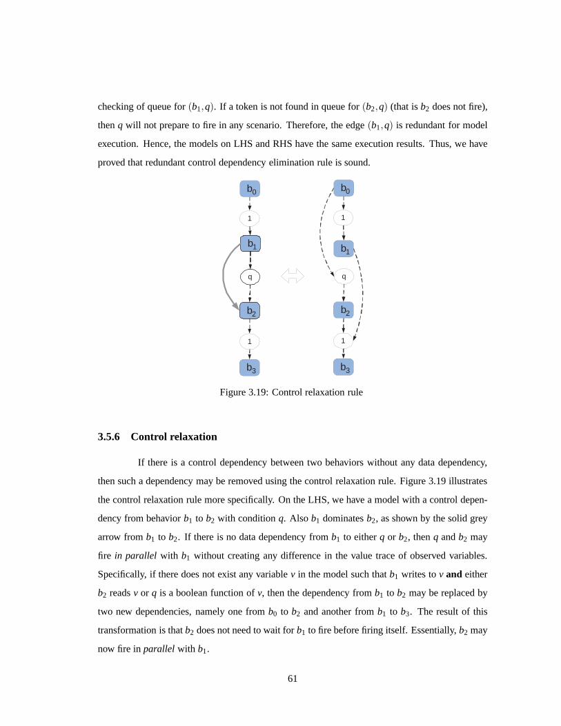
checking of queue for(b1,q). If a token is not found in queue for(b2,q) (that isb2 does not fire),

thenq will not prepare to fire in any scenario. Therefore, the edge(b1,q) is redundant for model

execution. Hence, the models on LHS and RHS have the same execution results. Thus, we have

proved that redundant control dependency elimination ruleis sound.

b 1

b 2

q

1

1

b 1

b 2

q

1

1

b 3

b 0 b 0

b 3

Figure 3.19: Control relaxation rule

3.5.6 Control relaxation

If there is a control dependency between two behaviors without any data dependency,

then such a dependency may be removed using the control relaxation rule. Figure 3.19 illustrates

the control relaxation rule more specifically. On the LHS, wehave a model with a control depen-

dency from behaviorb1 to b2 with conditionq. Also b1 dominatesb2, as shown by the solid grey

arrow fromb1 to b2. If there is no data dependency fromb1 to eitherq or b2, thenq andb2 may

fire in parallel with b1 without creating any difference in the value trace of observed variables.

Specifically, if there does not exist any variablev in the model such thatb1 writes tov and either

b2 readsv or q is a boolean function ofv, then the dependency fromb1 to b2 may be replaced by

two new dependencies, namely one fromb0 to b2 and another fromb1 to b3. The result of this

transformation is thatb2 does not need to wait forb1 to fire before firing itself. Essentially,b2 may

now fire inparallel with b1.

61

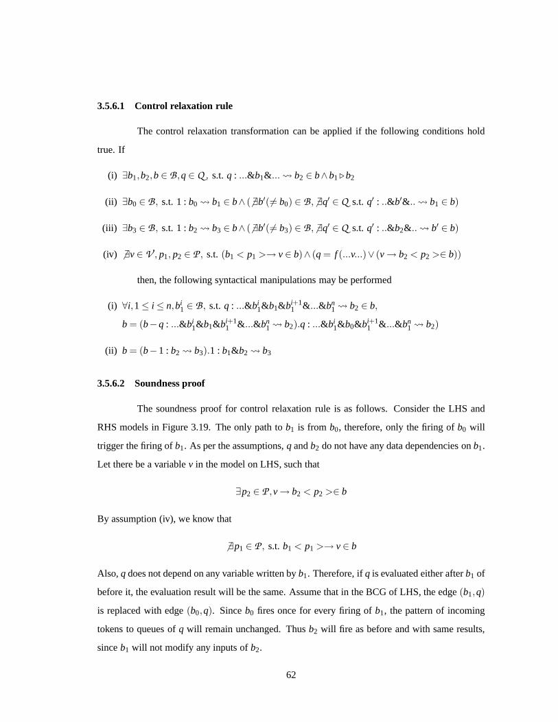
3.5.6.1 Control relaxation rule

The control relaxation transformation can be applied if thefollowing conditions hold

true. If

(i) ∃b1,b2,b∈ B ,q∈ Q , s.t. q : ...&b1& ... b2 ∈ b∧b1⊲b2

(ii) ∃b0 ∈ B , s.t. 1 :b0 b1 ∈ b∧ (6 ∃b′(6= b0) ∈ B , 6 ∃q′ ∈ Q s.t. q′ : ..&b′& .. b1 ∈ b)

(iii) ∃b3 ∈ B , s.t. 1 :b2 b3 ∈ b∧ (6 ∃b′(6= b3) ∈ B , 6 ∃q′ ∈ Q s.t. q′ : ..&b2& .. b′ ∈ b)

(iv) 6 ∃v∈ V , p1, p2 ∈ P , s.t. (b1 < p1 >→ v∈ b)∧ (q = f (...v...)∨ (v→ b2 < p2 >∈ b))

then, the following syntactical manipulations may be performed

(i) ∀i,1≤ i ≤ n,bi1 ∈ B , s.t. q : ...&bi

1&b1&bi+11 & ...&bn

1 b2 ∈ b,

b = (b−q : ...&bi1&b1&bi+1

1 & ...&bn1 b2).q : ...&bi

1&b0&bi+11 & ...&bn

1 b2)

(ii) b = (b−1 : b2 b3).1 : b1&b2 b3


The soundness proof for control relaxation rule is as follows. Consider the LHS and

RHS models in Figure 3.19. The only path tob1 is from b0, therefore, only the firing ofb0 will

trigger the firing ofb1. As per the assumptions,q andb2 do not have any data dependencies onb1.

Let there be a variablev in the model on LHS, such that

∃p2 ∈ P ,v→ b2 < p2 >∈ b

By assumption (iv), we know that

6 ∃p1 ∈ P , s.t. b1 < p1 >→ v∈ b

Also,q does not depend on any variable written byb1. Therefore, ifq is evaluated either afterb1 of

before it, the evaluation result will be the same. Assume that in the BCG of LHS, the edge(b1,q)

is replaced with edge(b0,q). Sinceb0 fires once for every firing ofb1, the pattern of incoming

tokens to queues ofq will remain unchanged. Thusb2 will fire as before and with same results,

sinceb1 will not modify any inputs ofb2.

62

Now consider the control node followingb2, with control condition 1. As per assump-

tion (iii), there are no other control nodes with an edge fromb2. Therefore, for every firing of

b2, the successor nodeb3 will also fire once. In the LHS model,b3 would fire if bothb1 andb2

would fire, sinceb2 ⊲b3. In the model on the RHS,b3 fires if bothb1 andb2 fire. This is ensured

by the extra control dependency added as an edge fromb1 to 1. Therefore, the execution of both

LHS and RHS will produce a different firing order of behaviors, but the same value traces for all

observed variables. Hence, the control relaxation rule is sound.

b 2

q

b 3

vsp

b 11

b

q

4

b 4

e

1 1

b 11 b 1n

b 1n

Figure 3.20: Streamlining rule

3.5.7 Streamlining

The streamlining rule is used to simplify the model algebraic expression by removing

redundant control dependencies. It is similar to control dependency elimination and identity elim-

ination and can be used in cases when neither of the above rules can be applied. As illustrated in

Figure 3.20, streamlining rule can be applied for a given control nodeq with successorb4 andn+1

predecessors, wheren≥ 1 one of the predecessors is an identity behaviore. Identitye, in turn has

two control dependencies (both with condition 1), from two behaviors, sayb2 andb3. Behaviorb2

is eitherVSPof the model or dominated byVSP. Behaviorb3 is eitherb4 or dominated byb4. If

b3 6= b4, thenb3 must fire at least oncebetweenany two firings ofb4. If all the conditions are met,

then the model may be transformed by removing the control dependency frome to b4, effectively

deleting the edge frome to q.

63

3.5.7.1 Streamlining rule

The streamlining transformation can be applied if the following conditions hold true. If

(i) ∀n≥ 1,∃b11,b12, ...,b1n,b2,b3,b4,e,b∈ B ,q∈ Q , s.t.

q : b11& ...&b1n&e b4 ∈ b∧1 : b2 e∈ b∧1 : b3 e∈ b

(ii) (b2 = vsp∨vsp⊲b2)∧ (b3 = b4∨ (b4 ⊲b3∧b3⊲ (b4,b4)))

then, the following syntactical manipulation may be performed

b = (b−q : b11& ...&b1n&e b4).q : b11& ...&b1n b4


The soundness proof for streamlining rule is performed by comparing the BCGs for the

models on the LHS and the RHS of Figure 3.20. In the model on theLHS, we have a control node

q with control edges from behaviorsb11 throughb1n and identitye. Also, q has a control edge to

behaviorb4. Now, from the execution semanticsb4 will fire if all of b11 throughb1n and identity

e fire and then conditionq evaluates to true. Let us consider the firing of identitye. Nodee has

two incoming control paths fromb1 andb2. Therefore,ewill fire if and only if eitherb1 of b2 fire.

From assumption (ii),b1 is eithervspor dominated by it. Therefore, during all of model execution

b1 will fire only once, sincevspfires only once for any model execution. Now, by the second part

of assumption (ii),b2 is either same asb4 or fires once for each firing ofb4 (after b4 has fired).

Therefore, the first firing ofewill result from the control path fromb1, leading to a potential firing

of b4, if all of b11 throughb1n fire. If b4 fires, thenb2 will also fire, leading to another firing ofe

and a subsequent potential firing ofb4 if all of b11 throughb1n fire. Therefore, every firing ofb4 is

dependent only on the firing ofb11 throughb1n and the evaluation ofq to be true. Thus, the control

dependency represented by the edge(e,q) is redundant. Hence, the models on both LHS and RHS

produce the same firing of behaviors. Since, no data relations are modified, we have proven the

soundness of streamlining rule.

64

3.6 Chapter Summary

In this chapter, we introduced a formalism called Model Algebra, which can be used for

functional verification of system level models. The objectsand composition rules of Model Al-

gebra allowed us to represent hierarchical system level models as expressions. We then presented

the formal execution semantics of model algebraic descriptions using behavior control graphs.

We also established a notion of functional equivalence of two models based on the value trace

of variables in the models. This led us to define functionality preserving transformation rules on

model algebraic descriptions. The soundness of these transformation rules was proved based on

our notion of equivalence. The expressive power and well defined rules in MA can be used to

derive new equivalent models from the specification and perform correct transformations on them.

The formalization of models using Model Algebra shows promise of significant impact on system

level verification.

65

Chapter 4

Functionality Preserving Refinements

In the last chapter we proposed a formalism for representingsystem level models as

expression. Within this formalism , called Model Algebra, we also defined a set of correct trans-

formation rules that can be used to derive an equivalent model from another model. In this chapter,

we will apply the established theory of Model Algebra to a real life system design methodology.

The design methodology is based on the SpecC methodology that starts with an exe-

cutable functional specification model of the design and is gradually refined into a cycle accurate

model that is ready to be manufactured using traditional design automation tools. The refinement

process consists of several steps. Each of these steps syntactically manipulates the model either

by rearranging or replacing objects in the model. We will identify the key refinement steps that

can be verified in Model Algebra and give algorithms for implementing such refinements. Proofs

of correctness for each refinement algorithms is based on thepreviously proven transformation

rules. These proofs will establish the correctness of the refinement algorithms and ensure that the

derived models are indeed functionally equivalent to the original models.

4.1 Refinement Based Design Methodology

A possible system level design methodology is illustrated in Figure 4.1. The designer

starts with a specification of the platform architecture in terms of components and system busses

and their connections. The functional specification is provided as an executable model. This

specification model forms the golden reference for all models in upcoming design steps. Based

66

Executable Specification Model

Design Decisions

Unscheduled Architecture Model

Scheduled Architecture Model

Transaction Level Model

Cycle Accurate Model

Behavior Partitioning

Serializing

Transaction Routing

SW Synthesis HW Synthesis Library of RTL components and Protocol Models

Library of RTOS and Protocol

Models

Serialized Architecture Model

Comm. Scheduling

Platform Spec.

System Level Design

Cycle Accurate Design

Figure 4.1: Refinement based design methodology

on the platform model and certain performance contraints for the system, the designer makes

decisions to refine the specification model in a step wise fashion. At each step, a model is changed

to reflect features of the platform, resulting in a new executable model, which can be further

refined.

The process of going from the purely functional specification model to a very detailed

cycle accurate model, that can be passed on to traditional design automation tools, is broadly di-

vided into two major design steps. The first is the system level design step that takes the functional

specification to a transaction level model. The transactionlevel model contains details pertaining

to the mapping of functional tasks to appropriate components and the routing of abstract commu-

nication over system busses. However, it does not have any information on the micro-architectural

67

details of the components and the busses themselves.

The transaction level model is handed off to the next step of cycle accurate (CA) design.

During CA design, the functional task mapped to hardware components undergo HW synthesis

to derive RTL models of the application and the bus interface. Similarly, for task mapped to

processors, we perform OS targeting and compilation to get aSW binary that can be down loaded

to the processor and simulated using the instruction set simulator of the processor.

Our work falls under the domain of system level design. Hence, in this dissertation, we

will concern ourselves with models and transformations that are encountered in going from func-

tional specification to transaction level. We will discuss four key refinements and their verification

in Model Algebra. These refinements are

1. Behavior Partitioning: During this refinement, the hierarchy of behaviors in the functional

model is rearranged to reflect the mapping of leaf level behaviors to component behaviors

[PAG02]. New transaction links may be introduced to allow data transfer between behaviors

mapped to different components or to synchronize between such behaviors. The refinement

is driven by the design decisions including mapping of behaviors to components and map-

ping of new transaction links to busses.

2. Serializing: In order to prepare the model for HW synthesis, behaviors that must be exe-

cuted with a single controller are serialized. The serialization refinement converts parallel

composition of relevant behaviors into sequential compositions.

3. Communication scheduling: The performance of a design may be improved by modify-

ing the scheduling of bus transactions [MDR+00]. The corresponding refinement process

reorders the communicating behaviors to reflect the scheduling decision.

4. Transaction routing: Transaction links may be reassigned from one bus to anotherto im-

prove performance. Sometimes, due to interface incompatibility, a bridge or router may

be inserted between communicating components [BK87]. Thisresults in the splitting of

a transaction link (between such components) into two links, one from the sender to the

router, and another from the router to the receiver. Functionally, the router is simply an

identity behavior that loops forever, reading from one linkand writing to another.

68

We will now look at each of the design steps in greater detail.Refinement algorithms

for deriving new models for each set of design decisions withalso be presented and proved using

rules of model algebra.

4.2 Behavior Partitioning

A given specification model may consist of an arbitrary hierarchy of behaviors. During

partitioning, we determine the number of processing elements (PEs) that will be needed to imple-

ment the design. The leaf behaviors in the specification are then distributed over these PEs. The

PEs are assumed to execute concurrently. Thus, in this step,the design decision is to map each leaf

behavior in the specification model to a PE. We will consider two different refinemnet algorithms

that create a different style of architecture model for the same design decisions. The styles differ

in the size of the models and the amount of synchronization required between PEs. However, both

algorithms will be proven to produce models that are functionally equivalent to the specification.

4.2.1 Design Decisions

The decision to implement a given task on a certain PE is determined by several factors.

Often, restrictions on the type of PE limit the choice of mapping. For example, a task involving

floating point operations is better implemented on a processor with a built in floating point unit.

Although the floating point operation may be emulated in software on a processor without a ded-

icated floating point unit, the performance of an emulated implementation is significantly poorer.

Another motivation for using multiple PEs may be to utilize the built in parallelism in the applica-

tion in order to improve preformance. Furthermore, most hard real time applications may require

a mix of SW processors and specialized HW components to meet both flexibility and performance

demands.

We now show how the design decisions are input to the refinement algorithm. LetMs

be the specification model that needs to be refined. LetLea f s(Ms) be the set of all leaf level

behaviors inMs. Let there ben different PEs in the platform architecture namedPE1 throughPEn.

Let mapi be the set of leaf behaviors inMs that are assigned for implementation on component

PEi, where 1≤ i ≤ n. The mapping is such that

69

1. A leaf behavior is mapped to only one PE, i.e.∀i, j1≤ i, j ≤ n, i 6= j,mapi ∩mapj = {}

2. All leaf behaviors are mapped to some PE, i.e.Si=n

i=1mapi = Lea f s(Ms)

The input to the refinement algorithm from the designer isn,mapi , where 1≤ i ≤ n.

4.2.2 Refinement Algorithm for Lock-Step output

The input to behavior partition refinement is the original specification model and the

design decision of mapping leaf level behaviors to the PEs. The goal is to generate a model

that represents the mapping of system functionality to architecture components. The specification

model is an arbitrary hierarchy of behaviors representing the system functionality. Model refine-

ment would distribute the behaviors onto components that run concurrently in the system. It must

be noted that refinement does not in any way influence the mapping decision. The designer is free

to choose any mapping of behaviors to components and refinement would produce a model that

represents it. However, each leaf behavior in the specification model must be mapped to only one

component.

Figure 4.2 shows the application of the lock-step refinementalgorithm on a behavior

bi of a given specification modelMs. The rule shown in the figure is applied generally to all the

behaviors in the specification. We assume that the architecture consists of two processing elements

PE1 and PE2. Letmap1 be the set of leaf level behaviors ofMs that are mapped to PE1 andmap2

be the set of leaf behaviors mapped to PE2. In the illustration, we have assumed thatbi ∈ map1.

The architecture modelMa is created as follows. We start by creating a parallel compo-

sition of all PEs, to denote the concurrent execution of PEs in the system. We have,

Ma = [PE1].[PE2]...[PEn].1 : vsp PE1...1 : vsp PEn.1 : PE1...PEn vt p

Then, we copy the specification model inside each PE. The leaflevel behaviors in each copy are

replaced by special hierarchical behaviors depending on the mapping. We will demonstrate this

replacement using the illustration in Figure 4.2. Sincebi is mapped to PE1, in the architecture

model Ma, we will replace copy ofbi inside PE1 withbi1, where hierarchical behaviorbi1 is

created as follows.

70

c bus

s i

b i

1

1

t i1

t im

v 1

v m

a 1

a m

a 1

a 1 a m a m

p 1

p m

a 0

a 0

a 0

b i1

p' 1

p' m

s' i

1

t' i1

t' im

v' 1

v' m

a 1

a m

b i2

p 1

p m

a 1

a m

a 0

a 1 a m a 0 a 0

PE2

bif

bif bif

bif

M s

b i

v 1

v m

p 1

p m

PE1

Figure 4.2: Lock-step style output of behavior partitioning refinement

Let Ms be the modelMs after flattening down to leaf behaviors. Let there be variables

v1 throughvm, such thatbi is a writer for all these variables. That is

∀ j,1≤ j ≤ m,∃bi → v j ∈ Ms

The hierarchical behaviorbi1 is a sequential composition ofm+2 behaviors namelysi ,bi , ti1, ..., tin,

where all these behaviors, exceptbi , are identity. We also copy the ports ofbi ontobi1, such that

port p on bi1 is mapped to portp on bi . Additionally, we createm new in ports onbi1, that allow

behaviorst1 throughtm to read the local copies of variablesv1 throughvm. We also create an extra

port bi f to work as the bus interface, which is mapped to channelcbus that represents the system

bus. Blocking write relations tobi f are added insidebi1 to synchronize its execution with other

PEs.

71

If a leaf behavior is not mapped to a PE, then its local copy inside the PE is replaced

by a special hierarchical behavior as follows. We will demostrate this case on the replacement

of bi inside PE2, sincebi 6∈ map2. Let bi be replaced bybi2 inside PE2 as follows. We create a

sequential composition ofm+1 identity behaviors namelys′i , t′i1, ..., t

′im. We also createm in ports

on bi2 corresponding to them out ports ofbi in Ms. The ports are mapped to the local copies of

the m variables that are written bybi in Ms. Insidebi2, the ports are mapped to the outputs of

the identity behaviorst1 throughtm. We also create an additionbi f port as in the previous case.

Blocking read relations are created usingbi f to all the identity behaviors insidebi2. The addressing

of these relations is done such thatsi sends a transaction tos′i labeleda0. Transactions for sending

variables written bybi to update the local copies in PE2 are created such that∀ j,1 ≤ j ≤ m, ti j

sends variablev j to t ′i j using transaction addresseda j overcbus.

The idea of the lock-step output is that each leaf behavior executes inside the PE it

was mapped to. Any outputs updated by the leaf behavior execution are immediately copied to

the local copies of the outputs inside other PEs. Behaviors following the execution of this leaf

behavior must wait until all the copies everywhere in the system are updated. Therefore, the state

of the system at leaf behavior boundaries is preserved in thearchitecture model.

The pseudo code for the lock-step style refinement is presented in Algorithm 2. The

algorithm uses a method calledEncapsulatethat is presented in Algorithm 1. TheEncapsulate

method is the inverse of flattening a hierarchical behavior with a single child behaviors.

4.2.3 Correctness Proof for Lock-Step Refinement

We now present the proof of correctness for the refinement algorithm for generating

lock-step style architecture model. LetMs be the specification model and letbi be a leaf level

behavior inMs. Assume that the designer mapsbi to PEk. In other words,bi ∈ mapk. Figure 4.3

shows the basic proof steps we follow. Our proof strategy is to take the generated architecture

model and use the functionality preserving transformationrules to derive the specification. The

illustration is for an architecture with two PEs, but the proof can be easily generalized to multiple

PEs.

We begin by using the flattening transformation rule to create a flattened architecture

model. Consider behaviorbi in the flattened architecture model as shown in Figure 4.3(a). By the

72

Algorithm 1 Encapsulte (Behavior b, Behavior Parent)1: be = [b].1 : vspe

b.1 : b vt pe

2: if ∀v∈ V , p∈ P ,v→ b ∈ Parent then

3: be = be.I → b 

4: end if

5: if ∀p, p′ ∈ P ,I < p′ >→ b ∈ Parent then

6: be = be.I → b 

7: end if

8: if ∀v∈ V , p∈ P ,b → v∈ Parent then

9: be = be.b → I 

10: end if

11: if ∀p, p′ ∈ P ,b → I < p′ >∈ Parent then

12: be = be.b → I 

13: end if

14: if ∀p, p′ ∈ P ,a∈ A ,a : I < p′ > 7→ b ∈ Parent then

15: be = be.a : I 7→ b 

16: end if

17: if ∀p, p′ ∈ P ,a∈ A ,a : b → I < p′ >∈ Parent then

18: be = be.a : b → I 

19: end if

20: if ∀p, p′ ∈ P ,a∈ A ,c∈ C ,b′ ∈ B ,c < a >: b′ < p′ > 7→ b ∈ Parent then

21: be = be.a : I 7→ b 

22: end if

23: if ∀p, p′ ∈ P ,a∈ A ,c∈ C ,b′ ∈ Bc < a >: b → b′ < p′ >∈ Parent then

24: be = be.a : b → I 

25: end if

26: Parent= Parent|b=be

73

Algorithm 2 Refine2LockStep (Ms,n,map1, ...,mapn)

1: Ms = f latten(Ms); Lea f s(Ms) = {b1,b2, ...}

2: for i = 1 TOn do

3: PEi = Ms; ∀v∈ vars(Ms),PEi = PEi|v=vi ; ∀q∈ ctrls(Ms),qi = q|v=vi ,PEi = PEi|q=qi

4: for j = 1 TO |Lea f s(Ms)| do

5: varsj = {v |b j → v∈ Ms∧ (∃q,q = f (...,v, ..)∨∃b 6∈ mapi ,v→ b < p′ >∈ Ms)

6: if b j ∈ mapi then

7: bij = Encapsulate(b j ,PEi)

8: bij = (bi

j −1 : vspij b j −1 : b j vt pi

j).1 : vspij si

j

9: bij = bi

j .aj0 : si

j < out > 7→ I < p0 > .1 : b j t ij1

10: for k = 1 TO |varsj | do

11: bij = bi

j .b j < pk >→ I < pk > .I < p′k >→ t ijk < in >

12: bij = bi

j .ajk : t i

jk < out > 7→ I < p0 > .1 : t ijk t i

j(k+1)

13: end for

14: bij = (bi

j −1 : t ij|varsj |

t ij(|varsj |+1)).1 : t i

j|varsj | vt pi

j

15: else

16: bij = 1 : vspi

j sij .a

jo : I < p0 > 7→ si

j < in >

17: last = sij

18: for k = 1 TO |varsj | do

19: if (∃q,q = f (...,varsj (k), ...))∨ (∃b′ ∈ mapi ,varsj (k) → b′ < p′ >∈ Ms) then

20: bij = bi

j .ajk : I < pk > 7→ t i

jk < in > .t ijk < out>→ I < pk > .1 : last t i

jk; last= t ijk

21: end if

22: end for

23: bij = bi

j .1 : last vt pij

24: end if

25: PEi = PEi|bj=bij

26: end for

27: Ma = Ma.[PEi].vsp PEi

28: end for

29: Ma = Ma.PE1&PE2& ...&PEn vt p

74

c bus

s i

b i

1

1

t i1

v 1 a 1

a 0

b i1

s' i

1

t' i1 v' 1

a 1

b i2 a 0

s i

b i

1

1

t i1

v 1

s' i

1

t' i1

v' 1 1

t i2

1

t' i2 1

1

t i2

t' i2

s i

b i

1

v 1

s' i

1

t' i1

1 1

t i2 t' i2

s i

b i

1

v 1

s' i

1 1

t i2 t' i2

s i

b i

1

v 1

s' i

1 1

t i2 t' i2

(a) (b)

(c) (d) (e)

Step 1

S t e p 2

Step 3 Step 4

Figure 4.3: Proof steps for refinement to lock-step style model

refinement results shown in Section 4.2.2, we have channel transactions fromsi to s′i , from t ′i1 to

ti1 and so on.

We apply the transaction link resolution rule to convert transaction links into new control

and data dependencies (Step 1). In this context, the link

c < a0 >: si < out > 7→ s′i < in >

is modified to the pair of control dependencies

1 : si&s′i bi .1 : si&s′i t ′i1

75

Similarly, the following link and data flow relation

c < a1 >: ti1 < out > 7→ t ′il < in > .t ′il < out >→ v′1

get converted to control dependencies and new data relations as follows

1 : ti1& t ′i1 ti2.1 : ti1& t ′i1 t ′i2.ti1 < out >→ v′1

The transformed model is shown in Figure 4.3(b). Next, we usevariable merging rule to merge

v1 andv′1 (Step 2). We have assumed here that concurrent behaviors maynot write to the same

variable. Thereforev′1 has no other writers exceptti1 and the condition for applying the variable

merging rule is met. Also, we eliminate identityti1 using Case (a) of the identity elimination rule.

As a result, we have the following new control relations added to the model

1 : bi& t ′i1 t ′i2.1 : bi& t ′i1 ti2

The resulting model is shown in Figure 4.3(c).

In Step 3, we optimize away identity behaviort ′i1 using Case (a) of the identity elim-

ination rule. The resulting model, shown in Figure 4.3(d) has the following new control flow

relations

1 : bi&si&s′i t ′i2.1 : bi&si&s′i ti2 (4.1)

It can be easily seen thatsi ⊲bi ands′i ⊲bi . Therefore, we can apply the RCDE rule to remove the

redundant control flow relations. Specifically, bothsi ands′i are removed as predecessors from

both control flow relations in 4.1. Therefore, we have the resulting model as shown in Figure

4.3(e).

We iteratively apply steps 1 through 4 over all the leaf levelbehaviors in the model,

thereby generalizing forbi . In the transformed model in 4.3(e), we can see that a relation

q : ...&bi& ... b j ∈ Ms

gets transformed into

1 : bi ti&1 : bi t ′i .q : ...& ti& ... sj .q : ...& t ′i & ... s′j .1 : sj&s′j b j ∈ Ma

76

Applying identity elimination onti , t ′i ,sj ,s′j , and RCDE we get

q : ...&bi& ... b j ∈ Ma

Therefore, we have

Ms = Ma ⇒ Ms = Ma

by soundness of flattening transformation rule. Hence Algorithm 2 is functionality preserving.

c bus

bif

a 1 i

a r i

a 1 o

a w o

1

o1 t

t ow

bif

v o1

v ow

i1 s

s ir

v i1

v ir a 1

i a r

i

a 1 o

a w o a 1

o

a w o

a 1 i

a r i

1

1 t

t w

PE2

bif

v' o1

v' ow

b i

1

1 s

s r v' i1

v' ir

a 1 i

a r i

a 1 o

a w o 1

1

vsp

a 1 o

a w o

a 1 i

a r i

1 q

n q

1 q'

m q'

PE1

b11

M s

b i

1 q

n q

1 q'

m q'

v i1

v ir

v o1

v ow

Figure 4.4: RPC style output of behavior partitioning refinement

4.2.4 Refinement Algorithm for RPC style output

The lock-step style output is easy to generate, but may result in too may inter-PE trans-

actions than needed. Some optimizations may be performed tominimize the number of such

77

transactions while keeping the functional equivalence of the input and output models. In the spe-

cial case, when a single behavior is mapped to a different PE,one may generate an optimal style

of architecture model that has very little inter-PE traffic.Essentially, the behavior mapped to the

different PE is triggered into execution as if it were a remote procedure call.

Figure 4.4 shows the output model generated when leaf level behaviorbi in the spec-

ification is mapped to PE2, when the rest of the specification is mapped to PE1. Therefore the

partitioning decision is such that

map1 = Lea f s(Ms)−{bi}; map2 = bi

In order to generate the architecture modelMa, we create a parallel composition of the two PEs as

follows

Ma = [PE1].[PE2].1 : vsp PE1.1 : vsp PE2.1 : PE1&PE2 vt p

The specification is copied inside PE1, as is, replacing onlybi with special hierarchical behavior

bi1. The behaviorbi1 is constructed as follows. LetMs be the specification model that has been

flattened down to its leaf level behaviors. Assume thatbi in Ms has r input ports mapped to

variablesvi1 throughvir . Also, let bi havew output ports, mapped to variablesvo1 throughvow

inside Ms. We createbi1 to be a sequential composition of(r + w) identity behaviors, namely

si1, ...,sir , to1, ..., tow in that order. We copy all the ports ofbi in Ms in bi1 and create port mappings

such thatkth in-port is mapped to in port of identitysik insidebi1. Similarly, thekth out port is

mapped to the out port of identitytok. Additionally, we create a bus interface portbi f on bi1. We

create blocking write and read relations insidebi1 as follows

∀k,1≤ k≤ r,aik : sik < out > 7→ I < bi f >

∀k,1≤ k≤ w,aok : I < bi f > 7→ tok < in >

On the other end inside PE2, we create a while loop with the body being a sequential

composition ofr + w+ 1 behaviors, namelys1, ...,sr ,bi , t1, ..., tw, in that order, where all the be-

haviors, exceptbi are identity. The loop runs endlessly over this body. We create copies of all

input and output variables ofbi in Ms inside PE2. Thekth input variables is mapped to the out port

of sk, while thekth output variable is mapped to the in port oftk. We also create blocking read and

78

write relations inside PE2 as follows

∀k,1≤ k≤ r,aik : I < bi f > 7→ sk < in >

∀k,1≤ k≤ r,aik : rk < out > 7→ I < bi f >

The RPC style output executes as follows. Wheneverbi is not executing, PE2 is waiting

on behaviors1 for a transaction from PE1. Inside PE1, whenever a control condition triggers

execution ofbi1, the sender identity behaviors insidebi1 send the input variables to PE2. Thus,

the local copies of the inputs ofbi are updated wheneverbi is scheduled to be executed. Once the

input gathering transactions are completed,bi executes and writes the outputs to PE2’s local copy

of bi ’s outputs. Then the sender identity behaviorst1 throughtw send the outputs to PE1, where

identitiesto1 throughtow update the local copies. The state of PE2 is back to waiting for the next

“call”. The execution seems to PE1 like a remote procedure call of bi , hence the name for the

model. The algorithm can be generalized to any number of PEs as long as PEs other than PE1

have only one behavior mapped to them. Algorithm 3 presents the pseudo code for refinement of

specification to an RPC style architecture model.

4.2.5 Correctness Proof for RPC Style Refinement

We now present the correctness proof for RPC style refinementalgorithm. Assume that

Ms is the specification model andbi is a leaf level behavior inMs. For simplicity, we will consider

the refinement for two PEs only. The proof can easily be generalized for more PEs. Let PE1

and PE2 by the two PEs in the system architecture. Let all leafbehaviors ofMs be mapped to

PE1, with the exception ofbi . Behaviorbi is mapped to PE2. Also, without loss of generality, we

assume thatbi has one input and one output. Figure 4.5(a) shows the flattened architecture model

for the said mapping.

We start by applying link resolution rule to eliminate channel cbus from the model and

introducing new control and data relations as follows (Step1). The transaction link and data

dependency relations

c < a0 >: si < out > 7→ s′i < in > .s′i < out >→ v′1

79

Algorithm 3 Refine2RPC (Ms,map1,map2)

1: PE1 = Ms = f latten(Ms)

2: Lea f s(Ms) = {b1,b2, ...}

3: for i = 1 TO |Lea f s(Ms)| do

4: inputsi = {v |∃p∈ P ,v→ bi ∈ Ms

5: out putsi = {v |∃p∈ P ,bi → v∈ Ms

6: if bi ∈ map2 then

7: last1 = vsp1i , last2 = vsp2

i

8: for j = 1 TO |inputsi | do

9: b1i = b1

i .1 : last1 s1i j .I < inpi j >→ s1

i j < in >

10: b1i = b1

i .ainj : s1

i j < out > 7→ I < bi f >

11: b2i = b2

i .1 : last2 s2i j .a

inj : I < bi f > 7→ s2

i j < in >

12: b2i = b2

i .s2i j < out >→ inv2

i j .inv2i j → bi < inpi j >

13: last1 = s1i j , last2 = s2

i j

14: end for

15: b2i = b2

i .1 : last2 bi ; last2 = bi

16: for k = 1 TO |out putsi | do

17: b1i = b1

i .1 : last1 t1ik.a

outk : I < bi f > 7→ t1

ik < in >

18: b1i = b1

i .t1ik < out >→ I < out pik >

19: b2i = b2

i .1 : last2 t2ik.bi < out pik >→ outv2

ik.outv2ik → t2

ik < in >

20: b2i = b2

i .aoutk : t2

ik < out > 7→ I < bi f >

21: last1 = t1ik, last2 = t2

ik

22: end for

23: b1i = b1

i .1 : last1 vt p1i ; b2

i = b2i .1 : last2 s2

i1

24: PE1 = PE1|bi=b1i; PE2 = PE2.[b2

i ].1 : vsp2 b2i

25: end if

26: end for

27: Ma = [PE1].[PE2].1 : vsp PE1.1 : vsp PE2.PE1&PE2 vt p

80

c bus

s i

1

t i1 a 1

a 0 s' i

1

t' i1

v' 1

a 1

a 0

1

t i2

1

(a)

Step 1

b i

1 v 2

v 1

v' 2

vsp

1 s i

1

t i1

s' i

1

t' i1

v' 1

1

t i2

1

(b)

b i

1 v 2

v 1

v' 2

vsp

1

s i

1

t i1

s' i

1

t' i1

v' 1

1

t i2

1

(c)

b i

1 v 2

v 1

v' 2

vsp

1

s i

1

t i1

1

t' i1

v' 1

1

t i2

(d)

b i

1 v 2

v 1

v' 2

Step 3

S t e p 2

s i

1

t' i1

v' 1

1

t i2

(e)

b i

1 v 2

v 1

v' 2

s i

1

1

t i2

(f)

b i

v 2

v 1 s i

1

1

t i2

(g)

b i

v 2

v 1

S t e p 4

Step 5 Step 6

Figure 4.5: Proof steps for refinement to RPC style model

81

are replaced by new control and data dependency relations

1 : si&s′i ti1.1 : si&s′i bi .1 : si < out >→ v′1

Also, the following relations

c < a1 >: t ′i1 < out > 7→ ti1 < in > .ti1 < out >→ v′2.1 : t ′i1 s′i

are replaced by

1 : ti1& t ′i1 ti2.1 : ti1& t ′i1 s′i .ti1′ < out >→ v′2

The resulting model is shown in figure 4.5(b).

Next, in Step 2, we use a generalization of streamlining transformation rule to remove

predecessors′i from the relation

1 : si&s′i bi (4.2)

The streamlining rule is applicable in this case sinces′i is identity and has two incoming control

relations. One relation has vsp as the predecessor. The other hasti1 andt ′i1 as the predecessors.

Looking at the control paths froms′i to ti1 andti1′ , it is easy to see that

bi ⊲ ti1∧ ti1⊲ (bi ,bi) and

bi ⊲ t ′i1∧ t ′i1⊲ (bi ,bi)

Therefore the streamlining rule may be applied to replace the relation in 4.2 by

1 : si bi

In Step 3, we again apply the streamlining rule, this time replacing

1 : si&s′i ti1

with

1 : si ti1

Sinces′i does not have any out-going edges and it is an identity behavior, it may be removed since

it does not modify any variables during model execution. Removal of s′i leads to the removal of

control conditions leading tos′i , thereby resulting in the cleaned up model in Figure 4.5(c).

82

Using identity elimination rule, we optimize away identitybehaviorsti1 andt ′i1 in steps

4 and 5, respectively. Before, optimizing awayt ′i1, we merge variablesv2 andv′2 using the variable

merging rule. Recall that we do not allow concurrent behaviors to write to the same variable.

Therefore, the variable merging rule is applicable in this case. Finally, sincesi dominatesbi , we

can perform RCDE transformation as shown in Step 6 to derive the model shown in Figure 4.5(g).

Now, by definition of the RPC style refinement algorithm, if there exists a relation

q : ...&b j& ... bi ∈ Ms

then in the architecture model, we will have

q : ...&b j& ... si ∈ Ma

Similarly, if we have

q′ : ...&bi& ... bk ∈ Ms

then in the architecture model, we will have

q′ : ...& ti& ... bk ∈ Ma

Now, from the result in Figure 4.5(g) and optimizing awaysi andti using identity elimination, we

have

q : ...&b j& ... bi ∈ Ma∧q : ...&bi& ... bk ∈ Ma

Therefore, we have

Ms = Ma ⇒ Ms = Ma

by soundness of flattening transformation rule. Hence, we have proved that behavior partitioning

refinement for RPC style output if functionality preserving.

4.3 Serializing

After mapping the different tasks in the specification to a set of processing elements,

we created a new model that reflected such a mapping. However,this new model might still not

be executable on the chosen platform. If we make the assumption that each PE in the system is

83

a uni-processor then we cannot handle the explicit task level parallelism in the model. In other

words, each PE can only have a single controller, therefore if we have any concurrently specified

tasks that are mapped to the same PE, then they need to be serialized. Alternately, the designer

may include an RTOS that serializes the tasks at run time.

In the context of Model Algebra, concurrent tasks are modeled as being explicitly par-

allel. If an underlying RTOS does run time thread creation and serialization [YGG03], then it

must be verified that the RTOS is indeed emulating the parallel specification as per our trace based

notion of equivalence. This requires property checking methods, which are beyond the scope of

this dissertation. In this section, we will discuss the refinement that statically serializes parallel

behaviors.


The design decision of mapping concurrent tasks to the same PE with static scheduling

implies the decision to serialize these tasks. Consider an unscheduled HW PE with two threads of

execution. The first thread executes behaviorb1 followed byb2, while the second thread executes

b3 followed by b4. A possible serialization of the PE would sequentially execute the behaviors

in the order{b1, b3, b2, b4}. Other schedules, that do not violate data dependencies, are also

possible.

We now formally define the design decision for serializing. Given a hierarchical behav-

ior b with parallel composition of its sub-behaviorsb1,b2, ...,bn. Therefore, we have the control

relations as

b = [b1].[b2]...[bn].1 : vsp b1...1 : vsp bn.1 : b1& ...&bn vt p

Let there be an ordered setO, with n integer variables such that

O = {o1,o2, ...,on}

Let there be an assignmentA of the integers inO such that eachoi ,1≤ i ≤ n is assigned a unique

integer between 1 andn. The serialization decision may be given as the setO and a serialization

refinement would modify the control condition of b, such thatafter refinement

b = [b1].[b2]...[bn].1 : vsp bo1.1 : vsp bo2...1 : vsp bon.1 : b1& ...&bn vt p

84

1 1

vsp

b 1 b n

1

1

1

b 1

1

b n

b par

b seq

vtp

vsp

vtp

Figure 4.6: Serialization of parallel behaviors

4.3.2 Refinement Algorithm

The goal is to generate a model that represents the new ordering of behaviors inside

components. Algorithm 4 gives the simple serialization refinement algorithm that serializes a

parallel composition according to user decisions. Withoutloss of generality, we can assume that

decision to simply be

∀1≤ i ≤ n,oi = i

Let there be a parallel composition of behaviors inside a hierarchical behaviorbpar in modelMs.

Let the child behaviors beb1,b2, ...,bn. Hence, we have

bpar = [b1]...[bn].1 : vsp b1...1 : vsp bn.1 : b1&b2& ...&bn vt p

Let Mser be the model after serialization ofbpar insideMs.

4.3.3 Proof of Correctness

We use induction and control relaxation rules of model algebra to prove the correctness

of serialization refinement. The induction step of the proofis shown in Figure 4.7. Assume we

85

Algorithm 4 Serialize (bpar,Ms)

1: Ms = f latten(Ms)

Require: 6 ∃v∈ V , i, j1≤ i, j ≤ n, i 6= j, s.t. bi < pi >→ v∈ Ms

Require: (v→ b j ∈ Ms∨b j → v∈ Ms)

2: bseq= bpar−1 : b1&b2& ...&bn vt p

3: last = vsp

4: for i = 1 TOn do

5: bseq= (bseq−1 : vsp bi)1 : last bi

6: last = bi

7: end for

8: bseq= bseq.1 : bn vt p

9: Mser = Ms|bpar=bseq

have a sequential composition of two behaviorsb1 andb2, such that there is no data dependency

between them. This includes variables that may be written byboth behaviors. We have

b = [b1].[b2].1 : vsp b1.1 : b1 b2.1 : b2 vt p

Since there is no data dependency betweenb1 andb2, we can use the control relaxation rule to

relax the dependency

1 : b1 b2

As a result, the transformed model is a parallel compositionas follows

b = [b1].[b2].1 : vsp b1.1 : vsp b2.1 : b1&b2 vt p

Hence, the parallel composition and sequential composition of b1 andb2 is equivalent. Therefore,

we have shown that serialization algorithm is functionality preserving for two behaviors.

Let us now consider a sequential composition ofn behaviors, namedb1 throughbn.

Assume that using control relaxation, we haveparallelizedthe firstm behaviorsb1 throughbm,

wherem< n, as shown in Figure 4.7. We now try to make a parallel composition of b1 through

bm+1.

Consider control flow relation

b1& ...&bm bm+1 (4.3)

86

1 1

vsp

b 1 b m

1

b

b m+1

1

1 1

vsp

b 1 b m

1

b

b m+1

1

1 1

vsp

b 1 b m

1

b

b m+1

1

Step 1 Step m

Figure 4.7: Inductive proof steps for serialization of parallel behaviors

Since there is no data dependency betweenb1 andbm+1, the control dependency fromb1 to bm+1

in 4.3 can be relaxed (Step 1). After control relaxation, we get the intermediate model as shown

in middle of Figure 4.7. The relation in 4.3 is replaced with two new control relations as follows

1 : vsp&b2& ...&bm bm+1.1 : b1&bm+1 bm+2

We continue to relax dependencies frombi to bm+1, where 1≤ i ≤ m. At the ith step, the control

relation in 4.3 is replaced by

1 : vsp&bi+1& ...&bm bm+1.1 : b1& ...&bi&bm+1 bm+2

This is because∀i,1≤ i ≤ m,bi does not have any data dependency onbm+1. Finally, at themth

step, we get the relations

1 : vsp bm+1.1 : b1& ...&bm+1 bm+2

We have shown that assuming the serialization algorithm is correct form, behaviors, it will also

be correct form+1 behaviors. Hence, we have proved in general that the serialization algorithm

is functionality preserving.

87

c bus

1

1

v

a a

bif bif

PE1

b 11

e 1

b 12

1

1 v'

PE2

b 21

e 2

b 22

a a c bus

1

1 v

a a bif

bif

PE1

b 11

b 12

1

1 v'

PE2

b 21

e 2

b 22

a

a

e 1

e 0 e' 0

a0 a0

a0 a0

e 0

a0

e' 0

a0

a0 a0

Figure 4.8: Different communication schedules for transaction over channelcbus.

4.4 Communication Scheduling

Once we have partitioned the behaviors and serialized them in their respective PEs, we

turn to optimization of inter PE communication. In a system with multiple PEs, point to point

communication may be shared over physical busses. Model Algebra, allows the specification of

bus based communication, by separating the logical transaction links from physical channels. A

single channel may support several logical point to point transaction links. Since channels have

built in arbitration, the transactions are ordered randomly at run time. We recall that for functional

verification, the actual arbitration scheme is irrelevant as long as it safe and fair. That is, no two

transaction requests will be granted together and no transaction request will be forever denied.

On of the important system level optimizations for communication performance is static

scheduling of transactions. Specifically, if two transactions are attempted concurrently on a given

bus, then it is difficult to predict from the model which transaction will be granted first. Therefore,

designer statically schedule transactions on the same bus to improve predictability of performance.

Essentially, this results in the reordering of behaviors that have channel transactions. Such a

scenario is shown in Figure 4.8, where datad is sent from PE1 to PE2 over channelc. The channel

implements rendezvous communication semantics, i.e. bothsender and receiver must synchronize

for the transaction to take place. Consequently, for the case shown in Figure 4.8(a),b12 must

wait until b21 has completed and the transaction is performed. Ifb21 takes a long time to execute,

execution inside PE1 will stall, as it waits for the data transaction. Behaviorb12 may be scheduled

88

before the transaction, if it has no data dependency one1 or . Of course, we are assuming thatb12

is a leaf level behavior without any blocking relations. Theresulting schedule,shown in 4.8(b),

optimizes timing so thatb12 does not have to wait for the transaction to complete.


The design decisions for communication scheduling are to advance or postpone a trans-

action depending on the schedule of bus transaction attempts and traffic [LDR01]. The transaction

may be advanced either by reordering the behaviors in the sender PE, such that the sender identity

is executed earlier. Alternately, the receiver identity may be scheduled earlier. The exact results of

the scheduling depend on run time data, so it cannot be guaranteed statically that a certain reorder-

ing would work better. The designer also has a limited windowfor scheduling the transaction.

For instance, the sender identity cannot be scheduled before the data to be sent is available. Con-

versely, the receiver identity cannot be scheduled after the variable that stores the received data is

read. Both these cases will result in erroneous simulation results.

The communication scheduling decisions can essentially begiven as a sequence of steps

of the following four types

1. Advance sender identity to executebeforeits current scheduled time

2. Postpone sender identity to executeafter its current scheduled time

3. Advance receiver identity to executebeforeits current scheduled time

4. Postpone receiver identity to executeafter its current scheduled time


The goal of communication scheduling refinement is to generate a model that repre-

sents the new ordering of behaviors and transactions. We present here four refinement algorithms

for the four types of design decisions. Algorithm 5 advancesthe sender identity before its cur-

rent schedule by exchanging its position with the immediately preceding behavior in the control

flow. Algorithm 6 postpones the execution of sender identityby exchanging its position with the

behavior scheduled immediately after the sender in the control flow. Algorithm 7 advances the

89

receiver identity before its current schedule by exchanging its position with the immediately pre-

ceding behavior in the control flow. Algorithm 8 postpones the execution of receiver identity by

exchanging its position with the behavior scheduled immediately after the receiver in the control

flow. All these refinement methods require that there is no data dependency between the identity

and the behavior it exchanges position with. Also, we require that there is a synchronization trans-

action before either of the exchanged behaviors. Also, the behavior must be leaf level and have no

blocking relations.

Algorithm 5 MoveSenderUp (Identitye, Behaviorb, BehaviorPE)

Require: ∃v∈ V ,a∈ A , s.tv→ e< in >∈ PE,a : e< out > 7→ I < bi f >∈ PE

Require: 1 : b e∈ PE, 6 ∃b′(6= b, 6= e) ∈ B ,q′ ∈ Q , s.t.

q′ : ...&b′& ... e∈ PE∨q′ : ...&b& ... b′

Require: 6 ∃a′ ∈ A , p∈ P , s.t. a : b 7→ I < bi f >∈ PE∨

a : I < bi f > 7→ b ∈ PE∨b → v∈ PE

1: for all q∈ Q , s.t. q : b1& ...&bn b∈ PE do

2: PE = (PE−q : b1& ...&bn b).q : b1& ...&bn e

3: end for

4: for all q∈ Q ,b′ ∈ B , s.t. q : ...&e& ... b′ ∈ PE do

5: PE = (PE−q : ...&e& ... b′).q : ...&b& ... b′

6: end for

7: PE = (PE−1 : b e).1 : e b


The proof steps for correctness of communication scheduling refinement are presented

in Figure 4.9. In this proof, we only consider the refinement that moves the communicating

behavior down on the sender component. The other three casescan be proved similarly.

We start with a flattened model for the one shown in LHS of Figure 4.8. The model has

sequentially executing behaviors on both the sender and receiver PE. We see two transactions over

the channelcbus, one at the top betweene0 ande′0, labeleda0 and one betweene1 ande2, labeled

a. We are trying to postpone the schedule of the latter transaction. It is assumed that there are

90

Algorithm 6 MoveSenderDown (Identitye,Behaviorb,BehaviorPE)

Require: ∃v∈ V ,a∈ A , s.tv→ e< in >∈ PE,a : e< out > 7→ I < bi f >∈ PE

Require: 1 : e b∈ PE, 6 ∃b′(6= e, 6= b) ∈ B ,q′ ∈ Q , s.t.

q′ : ...&b′& ... b∈ PE∨q′ : ...&e& ... b′


a : I < bi f > 7→ b ∈ PE∨b → v∈ PE

1: for all q∈ Q , s.t. q : b1& ...&bn e∈ PE do

2: PE = (PE−q : b1& ...&bn e).q : b1& ...&bn b

3: end for

4: for all q∈ Q ,b′ ∈ B , s.t. q : ...&b& ... b′ ∈ PE do

5: PE = (PE−q : ...&b& ... b′).q : ...&e& ... b′

6: end for

7: PE = (PE−1 : e b).1 : b e

Algorithm 7 MoveReceiverUp (Identitye,Behaviorb,BehaviorPE)

Require: ∃v∈ V ,a∈ A , s.te< out >→ v∈ PE,a : I < bi f > 7→ e< in >∈ PE

Require: 1 : b e∈ PE, 6 ∃b′(6= b, 6= e) ∈ B ,q′ ∈ Q , s.t.

q′ : ...&b′& ... e∈ PE∨q′ : ...&b& ... b′


a : I < bi f > 7→ b ∈ PE∨v→ b ∈ PE

1: for all q∈ Q , s.t. q : b1& ...&bn b∈ PE do

2: PE = (PE−q : b1& ...&bn b).q : b1& ...&bn e

3: end for

4: for all q∈ Q ,b′ ∈ B , s.t. q : ...&e& ... b′ ∈ PE do

5: PE = (PE−q : ...&e& ... b′).q : ...&b& ... b′

6: end for

7: PE = (PE−1 : b e).1 : e b

91

S t e p 2

c bus

1

1

v

a a

bif bif

b 11

e 1

b 12

1

1 v'

b 21

e 2

b 22

a a

e 0 e' 0

a0 a0

a0 a0

Step 1

1

1

b 11

e 1

b 12

1

1

b 21

e 2

b 22

e 0 e' 0

v

v'

1

b 13

1

b 13

1

1

b 11

e 1

b 12

1

1

b 21

e 2

b 22

e 0 e' 0

v

v'

1

b 13

Step 3 1

1

b 11

e 1

b 12

1

1

b 21

e 2

b 22

e 0 e' 0

v

v'

1

b 13

1

1

b 11

e 1

b 12

1

1

b 21

e 2

b 22

e 0 e' 0

v

v'

1

b 13

S t e p 4

1

1

b 11

e 1

b 12

1

1

b 21

e 2

b 22

e 0 e' 0

v

v' 1

b 13

Step 5

(a)

(b)

(c) (d)

(e) (f)

Figure 4.9: Proof steps for verification of communication scheduling

92

Algorithm 8 MoveReceiverDown (Identitye,Behaviorb,BehaviorPE)

Require: ∃v∈ V ,a∈ A , s.te< out >→ v∈ PE,a : I < bi f > 7→ e< in >∈ PE

Require: 1 : e b∈ PE, 6 ∃b′(6= e, 6= b) ∈ B ,q′ ∈ Q , s.t.

q′ : ...&b′& ... b∈ PE∨q′ : ...&e& ... b′


a : I < bi f > 7→ b ∈ PE∨v→ b ∈ PE

1: for all q∈ Q , s.t. q : b1& ...&bn e∈ PE do

2: PE = (PE−q : b1& ...&bn e).q : b1& ...&bn b

3: end for

4: for all q∈ Q ,b′ ∈ B , s.t. q : ...&b& ... b′ ∈ PE do

5: PE = (PE−q : ...&b& ... b′).q : ...&e& ... b′

6: end for

7: PE = (PE−1 : e b).1 : b e

sequential paths frome0 ande′0 to b11 andb21 respectively. Therefore, we have

(e0 ⊲b11)∧ (e′0 ⊲b21)∧ (e0⊲b21)∧ (e′0⊲b11) (4.4)

After applying link resolution rule (Step1), the transaction and data relation

cbus< a >: e1 < out > 7→ e2 < in > .e2 < out >→ v′

is converted to appropriate control and data relations

1 : e1&e2 b12.1 : e1&e2 b22.e1 < out >→ v′

It can be seen from the model that there are no data dependencies from eithere1 or e2 to b12.

Therefore, in Step 2, we relax these control dependencies using the control relaxation rule. The

resulting model is shown in Figure 4.9(c). Now, we have a control dependency fromb21 to b12.

Assuming that there are no shared memories between the two components, then we can assume

that there is no data dependency betweenb21 andb12. Thus, the control dependency can be relaxed.

After relaxation, there will be a control dependency onb12 from a behavior that executes before

b21. We continue to relax control dependencies onb12 until we get a dependency frome′0. This is

guaranteed to happen since there is a sequential composition in the receiver component.

93

In step 4, we use the result in 4.4 to remove the redundant control dependency onb12

from e′0. The application of RCDE is possible since we have the control dependency as

1 : b11&e′0 b12

Also, we can use RCDE on the control condition

1 : b21&e2 b13

because clearlyb21 ⊲e2. The resulting model is shown in 4.9(e). We can see that the sequential

relation betweene1 and b12 is now transformed to a parallel relation. Since these two donot

have any data dependencies, we can use the inverse of the control relaxation rule to derive the

model shown in Figure 4.9(f). This is isomorphic to the modelthat we get by flattening and

resolving the transaction links of model shown in RHS of Figure 4.8. Therefore, we have shown

that communication scheduling refinement is functionalitypreserving.

4.5 Transaction Routing

After behavior partitioning and scheduling, the system model consists of concurrent

behaviors communicating with several channels. Although,the model shows the computation

structure correctly, the communication structure still needs to be implemented. In a bus-based

SoC communication scheme, the various PEs are connected to system busses. The communication

model can thus be represented using channels for busses. Alltransaction links in the input model

are shared over the newbus channels.


The design decision in this case is choosing the number of buschannels and mapping the

transaction links to the bus channels. In some cases, a transaction link may need to be implemented

on several busses. This will require the addition of new identity behaviors to act as transducers,

that will allow the routing of transactions over busses.

94

e T1

1

vsp

1

e Tn

1

1

e' T1 e' Tn

1 1 v v

c bus1 a 1

a n

c bus2

a 1 a n

a 1 a n a n

a 1

bif1

bif2

v1 bif PE1

e 1

a 1

vn

bif

PE1

e n

a n

a 1

a n

bif vn'

PEn'

e' n

a n a n

bif v1'

PE1'

e' 1

a 1

a 1

Transducer

c bus1

v1

bif

PE1

e 1 a 1

vn

bif

PE1

e n

a n

a 1

a n

bif vn'

PEn'

e' n

a n a n

bif v1'

PE1'

e' 1

a 1

a 1

e'’ T1

1

a' 1

e' 1

a' 1

a' 1

a' 1 a' n

e'’ Tn

1

a' n

To bif1

a' n

e' n

a' n

Figure 4.10: Routing transactions via transducer


Let there be a modelMs of a system with a bus represented by channelc. Let there be

n transactions overc from and to different PEs connected toc. Suppose we change the commu-

nication architecture such that the communicating PEs are now connected to two different busses,

represented by channelsc1 and c2. The original transaction links represented by addressesa1

throughan must now go over two bussesc1 andc2, via a new component called theTransducer.

The transducer has two interfacesbi f1 andbi f2 for the two bussesc1 andc2, respectively. Inside

the transducer, we have a parallel composition ofn sets of 3 identity behaviors, each set responsi-

ble for routing of transactions on one original link. A set consists of a receiver identity behavior

that copies the incoming data from one bus into a local buffer, and a sender identity behavior that

95

sends the data from buffer over the other bus to the intended recipient and a notification identity be-

havior that sends a notification transaction to the sender after the sender has executed. Algorithm

9 gives pseudo code for the refinement resulting from transducer insertion.

Algorithm 9 InsertTransducer (Addressa1, ...an,Channelc,c1,c2,BehaviorMs)1: Ms = Ms.[T].1 : vsp T

2: for i = 1to TO n do

Require: ∃PEs,PEr ∈ B , s.t. c < ai >: PEs < bi f > 7→ PRr < bi f >∈ Ms

3: if (ConnectedTo(PEs) == bus1∧ConnectedTo(PEr ) == bus2) then

4: Ms = (Ms−c< ai >: PEs< bi f > 7→PRr < bi f >).c1 < a1i >: PEs< bi f > 7→T < bi f1 >

5: Ms = Ms.c2 < a2i >: T < bi f2 > 7→ PRr < bi f >

6: T = T.1 : vspT eTi.1 : eTi e′Ti.1 : e′Ti e′′Ti.1 : e′′Ti eTi

7: T = T.eTi < out >→ vi .vi → e′Ti < in >

8: T = T.a1i : I < bi f1 > 7→ eTi < in > .a2

i : e′Ti < out > 7→ I < bi f2 > .a3i : e′′Ti < out > 7→

I < bi f1 >

9: else if(ConnectedTo(PEs) == bus2∧ConnectedTo(PEr ) == bus1) then

10: Ms = (Ms−c< ai >: PEs< bi f > 7→PRr < bi f >).c2 < a1i >: PEs< bi f > 7→T < bi f2 >

11: Ms = Ms.c1 < a2i >: T < bi f1 > 7→ PRr < bi f >

12: T = T.1 : vspT eTi.1 : eTi e′Ti.1 : e′Ti eTi

13: T = T.eTi < out >→ vi .vi → e′Ti < in >

14: T = T.a2i : I < bi f2 > 7→ eTi < in > .a1

i : e′Ti < out > 7→ I < bi f1 >

15: end if

16: end for


Figure 4.11 shows the basic proof steps for showing equivalence between models before

and after transducer insertion. Without loss of generality, we assume a transducer between two

channelsc1 andc2 as shown in the flattened model in Figure 4.11(a). The transducer replaces a

direct channel transaction between identitiese1 ande2. The transducer consists of an endless loop

with a sequential body of 3 identities namelyeT , e′T ande′′T . IdentityeT has a transaction link from

96

e1. After this transaction occurs,eT copies the received data in a local variablev. Thusv is a copy

of v1. Then,e′T executes, sending data fromv to e2 over channelc2. Finally, after this transaction

is complete, identitye′′T executes and synchronizes withe′1

We start by resolving all the transaction links in the model into appropriate control and

data dependency relations using the link resolution transformation rule (Step 1). By the application

of this rule, we replace transaction and data relations

c1 < a1 >: e1 < out > 7→ eT < in > .eT < out >→ v

with the following relations

1 : e1&eT e′T .1 : e1&eT e′1.e1 < out >→ v

Transaction relations betweene′T ande2 and data relations ofe2 as follows

c2 < a2 >: e′T < out > 7→ e2 < in > .e2 < out >→ v2

are replaced by control and data relations

1 : e2&e′T e′′T .1 : e2&e′T e′2.e2 < out >→ v2

The notification transaction betweene′1 ande′′T is also replaced similarly using the link resolution

rule. At the end of transformations of Step 1, the model lookslike as shown in Figure 4.11(b).

In Step 2, we apply the streamlining rule in the same fashion as used in the proof for

RPC style behavior partitioning algorithm. The rule eliminated control dependencies fromeT to

e′1 and fromeT to e′t . As a result,eT does not have anything executing after it and it does not

modify and variable in the model, so it is removed from the model along with all its control and

data relation. The resulting model after this transformation is showed in Figure 4.11(c).

In Step 3, we optimize away identitiese′T ande′1 using the identity elimination rule. In

Step 4, we use the RCDE rule to remove the redundant control dependency frome1 to e′′1. This is

because the control dependency is cause by the relation

1 : e1&e′′T e′′1

ande1 ⊲e′′T , there by allowing application of RCDE. Finally, in Step 5, we optimize away identity

e′′T using the identity elimination rule. The final resulting model, as shown in Figure 4.11(f), is

97

c1

e 1

1

e' 1

a 1

e T

1 v 1

(a)

Step 1

v 1

e' T

a 1

c2 a 2 a 2

1

e' 2

e 2

v 2

e 1

1

e' 1

e T

1 1

(b)

v 1

e' T

1

e' 2

e 2

vsp

1

vsp

1

1

e'’ T

a 3

a 3

1

e'’ T

1

e'’ 1

1

e'’ 1

e 1

1

e' 1

1

(c)

v 1

e' T

1

e' 2

e 2

1

e'’ T

1

e'’ 1

Step 2

e 1

(d)

v 1

1

e' 2

e 2

1

e'’ T 1

e'’ 1

e 1

(e)

v 1

1

e' 2

e 2

1

e'’ T 1

e'’ 1

e 1

(f)

v 1

1

e' 2

e 2

1

e'’ 1

S t e p 3

Step 4 Step 5

v

v 2

v

Figure 4.11: Proof steps for transducer insertion during transaction routing refinement

98

identical to the one derived after link resolution of a direct link from e1 to e2. Therefore, we have

proved that the transducer insertion algorithm is functionality preserving.

4.6 Chapter Summary

In the last chapter, we had introduced our system level formalism and etablished func-

tionality preserving transformation rules in that formalism. In this chapter, we built upon that

theory to present some useful system level refinements. The refinement algorithms were proven

for correctness using the transformation rules of Model Algebra.

We presented the behavior partitioning refinements that come in two flavors. Based

on the design decision of mapping the tasks in a functional specification to different processing

elements (PEs), the refinement algorithms generated two different types of output models that

reflected the mapping. The first output model was based on the lock-step style of synchronization,

where the state of each PE is synchronized with other PEs. Thesecond output model employed a

remote procedure call style of synchronization, where the master PE used a channel transaction to

start execution of a behavior mapped to a slave PE. After execution, the slave PE returns to wait

for the next request from the master.

We then presented two commonly used refinements for scheduling tasks in different

PEs in the system. The first refinement was used to serialize parallel tasks if the designer wants

to minimize the number of controllers. The second refinementused reordering of communicating

behaviors to change the overall communication schedule in the system. Communication schedul-

ing is used to minimize the number of competing transactionson the bus, which in turn leads to

fewer arbitration delays and more predictable system behavior.

Finally, we presented a refinement resulting from changes tothe communication archi-

tecture in the system. If two communicating PEs have different interface structure or protocol,

then they cannot use the a single bus for communication. The transactions between such PEs must

be routed through a special bridge behavior that we refer to as a transducer. We showed how a

system model may be refined to insert transducers between PEswith incompatible interfaces.

All the aforementioned refinements were proved correct using the rules of Model Alge-

bra. In our design methodology, such refinements are frequently used to evaluate different system

99

architectures. Reliable methods for implementing these refinements cut the costs for verifying all

refined models that are generated during the system level design process.

100

Chapter 5

Automatic Refinement Verification

In the previous chapter we established theoretical resultspertaining to the refinement

of system level models in Model Algebra and the verification of such refinments. We used the

proof strategies for showing correctness of refinements to develop an automatic tool that applies

the sound transformation rules of model algebra on two models to prove their functional equiva-

lence. The models themselves are abstractions of performance models written in system design

languages, in our case SpecC.

Our verification methodology is shown in Figure 5.1. It follows from our system level

design methodology already discussed in the previous chapter and shown in Figure 4.1. We use

our automatic tool to check the equivalence of the models that udergo various refinements in

out methodology. In this chapter, we will present our equivalence verification tool, discuss the

automatic verification algorithms and provide experimental results for the verification tool on

SpecC examples.

The verification tool flow is shown in Figure 5.2. First, we abstract the SLDL model into

a graphical MA representation. The MA representation then undergoes a series of transformations

until no more transformations can be applied. The final modelis said to be normalized. The

normalized models are then checked for isomorphism. There are two key requirements for such a

verification technique to succeed. The first requirement is thesoundnessof the transformation laws

that are used to normalize the model. Soundness means that each transformation must produce

an equivalent model, according to the equivalence notion defined above. The second requirement

101

Executable Specification Model

Unscheduled Architecture Model

Scheduled Architecture Model

Transaction Level Model

Behavior Partitioning

Serializing

Transaction Routing

Serialized Architecture Model

Comm. Scheduling

Refinement Verifier

Refinement Verifier

Refinement Verifier

Refinement Verifier

Library of Transformation

Rules

Figure 5.1: Refinement Verification methodology

is that the normalization algorithm must always produce isomorphic normal forms for any two

models that can be proven equivalent using the transformation laws.

5.1 Functional Abstraction

Our verification tool is based on the syntax and semantics of Model Algebra. However,

it would be inconvenient and complicated for verification engineers to convert their system level

models into model algebraic expressions for verification. The key difference between a model

written in a typical SLDL and once written in Model Algebra isthat the model algebraic model

treats behaviors as black boxes or uninterpreted functions. Also, it treats any conditional expres-

sions in the model as uninterpreted predicates. The SLDL model evaluates values of variables

during execution, while in model algebra, we only care aboutthe interactions and dependencies of

the behaviors, conditions and variables. Therefore, a reasonable approach would be to automati-

102

Original SL Model (A)

Refined SL Model (B)

Functional Abstraction

Graphical Representation

(A)

Graph Normalization

Normalized Model A

Functional Abstraction

Graphical Representation

(B)

Graph Normalization

Normalized Model B

Isomorphism Check

Equivalent / Not Equivalent

Model Refinement

Figure 5.2: Steps in refinement verification

cally derive the model algebraic expression from an SLDL model.

The front end or our tool is essentially a SpecC parser that creates model algebraic

expressions from SpecC behaviors. In this section, we will give a brief overview of the relevant

features of SpecC and show how a SpecC behavior is abstractedinto a model algebraic behavior.

5.1.1 SpecC language and SIR

SpecC is a system design language that was created for modeling of embedded systems

consisting of tasks that run in HW and those that run in SW. It is built on top of ANSI-C and

allows explicit modeling of concurrency, bit-vector typesand hierarchy to allow system level rep-

resentation of HW/SW designs. We now look at the basic structure of SpecC language that are

relevant for our model algebra based functional verification. We also discuss the SIR application

programming interface that allows us to interpret and manipulate SpecC models. In our verifica-

tion tool, the key idea of functional abstraction module is to derive the model algebraic expression

of a design from its SpecC representation.

5.1.1.1 Basic Structure of SpecC

SpecC allows us to code a hierarchical composition of communicating behaviors. Each

behavior is either a module written in ANSI-C or a further composition of other behaviors. We

will not consider hierarchical behaviors that have sub-behaviors interspersed with other C-code.

It is perfectly legitimate to write and execute such a model,but defeats the purpose of clean

hierarchy and treatment of leaf behaviors as uninterpretedfunctions. SpecC allows for ports and

103

variables that have identical interpretation as ports and variables in MA. However, in SpecC,

ports and variables may have data types, something that is not considered in MA. In general,

channels in SpecC are different from those in MA since SpecC syntax considers a channel to be

simply a class with available functions. These functions may be declared in an interface that is

implemented by that channel. It is possible to have channelswith functions for purposes other than

communication, which would make them like any other behavior in MA. We will consider only

one implementation of the SpecC channel, namely the double handshake channel with mutually

exclusive data transfers. The semantics of the channel havealready been discussed in previous

sections. This channel can be easily written in SpecC and is assumed to be available in the models

that we are trying to verify. No other types of channels are allowed.

5.1.1.2 SpecC Internal Representation

The SpecC internal representation (SIR) is an abstract syntax representation of a model

written with SpecC syntax. The SIR also comes with a rich API for reading and modifying SpecC

programs. The functional abstraction module uses the SIR API to read a SpecC model and build

the verifier’s internal data structure representing the hierarchical model algebraic expression of the

model. SIR API provides the following classes and types thatfacilitate creation of model alge-

braic expressions.sir behavior::BehaviorClassused to identity if a behavior is to be treated as

uninterpreted function or a hierarchical behavior. Control relations are created based on the re-

turned behavior type.Classes forsir portmap and sirportdirectionused to identify port mappings

and the corresponding data flow relations.Inside FSM behaviorssir transitionsare used to create

control relations with complex control conditions.

5.1.2 Executable Performance Models in SpecC

A typical executable performance model is shown in Figure 5.3(a). The platform con-

sists of a processor (Proc.) connected to Bus1 along with twohardware components (HW1 and

HW2). Communication elements such as arbiter and interruptcontroller (IC) allow safe and syn-

chronized communication between the processor and the HW components. The architecture in

the model is captured using hierarchy (a parallel composition of components) and signals and

104

b1 b2

1

1

vsp

vtp

Bus1 b3

b4

1

1

!q

vsp

vtp

q

1

v

b3

1

1

vsp

vtp

vsp

1

1 1

1

l1

l2

l1

l2 Proc.

HW1 HW2

System

Proc.

Task Sched.

Driver

b1 b2

IC

HW1

b3

b4

Bus I/F

b5

Bus I/F HW2

Bus 1

Arbiter

vtp

(a) Performance Model (b) Abstract functional model

Figure 5.3: The platform model and its corresponding functional abstraction

channels for wires and bus interfaces. The application itself is captured by instantiating behaviors

inside the appropriate component behavior. For instance, behaviorsb1 andb2 of the application

are mapped to Proc. as seen by the behavioral hierarchy.

5.1.3 Deriving Model Algebraic Expression

Given the syntax of Model Algebraic representation, we derive the abstract functional

model of our example as shown in Figure 5.3(b). The bold grey arrows show the abstraction

of the objects in the performance model in Figure 5.3(a) intoobjects in the abstract model on

the right hand side. All hierarchical behaviors have uniquestart and terminate identity behaviors

calledvirtual starting point (vsp)andvirtual terminating point (vtp)respectively. Leaf behaviors

are copied as is since they are treated as uninterpreted functions. Sequentiality and loops inside

HW1 are modeled using control dependencies as shown. Note the abstraction of the behaviors

and the task scheduler inside Proc. using the control flow of MA. Both behaviorsb1 andb2 are

allowed to start simultaneous aftervsp. However, the Proc. behavior terminates only after both

b1 andb2 have terminated. All communication implemented in the performance model (using bus

signals, arbiter, IC, drivers and bus interfaces) is abstracted into high level transaction linksl1 and

l2 implemented on the channel labeledBus1. Finally, the top level system is abstracted as a parallel

composition of hierarchical component behaviors.

105

b:MA_Behavior

b1:MA_Behavior b2:MA_Behavior

c1:MA_Channel c2:MA_Channel

v1:MA_Variable v2:MA_Variable

q1:MA_Condition q2:MA_Condition

a1:MA_Address a2:MA_Address

p1:MA_Port p2:MA_Port

qv1:MA_CondVal qv2:MA_CondVal

rc1:MA_RC rc2:MA_RC

rnw1:MA_RNW rnw2:MA_RNW

rnwi1:MA_RNWI rnwi2:MA_RNWI

dep_v1:MA_Variable dep_v2:MA_Variable

dep_p1:MA_Port dep_p2:MA_Port

qv:MA_CondVal

bddvar:BDD

q:MA_Condition

pred1:MA_Behavior pred2:MA_Behavior

succ:MA_Behavior

source:MA_Port

destn:MA_Variable

source:MA_Port

destn:MA_Port

Figure 5.4: Data structure for storing model algebraic expression

106

b:MA_Behavior

rnr1:MA_RNR rnr2:MA_RNR

rbw1:MA_RBW rbw2:MA_RBW

rbr1:MA_RBR rbr2:MA_RBR

rnri1:MA_RNRI rnri2:MA_RNRI

rt1:MA_RT rt2:MA_RT

source:MA_Variable

destn:MA_Port

source:MA_Port

destn:MA_Port

source:MA_Port

destn:MA_Port

a:MA_Address

source:MA_Port

destn:MA_Port

a:MA_Address

source:MA_Port

a:MA_Address

destn1:MA_Port destn2:MA_Port

Figure 5.5: Data structure for storing model algebraic expression (contd.)

107

5.1.3.1 Internal representation for MA

In MA, the model is simply the top level behavior. In Figures 5.4 and 5.5, we have

shown the data structure for organizing model algebraic expression of a behavior. Each object and

composition rule in MA (excluding interface) has a unique class implementation. Additionally,

we have a class for boolean functions that are used for representing the values inside control con-

ditions. These boolean functions are stored and manipulated using BDDs in the CUDD package

and its application programming interface [CUD].

5.1.3.2 Translation from SpecC to MA

The system model in SpecC is a hierarchical composition of behaviors using different

composition styles such as sequential, parallel, FSM and pipeline. The behaviors at the same scope

communicate with variables or channels. Across hierarchies, ports facilitate behavior communi-

cation. There is a direct translation possible from a subsetof SpecC to MA. We will assume that

for synthesis and refinement purposes, the designers uses only those constructs that are allowed in

MA. All other SpecC constructs such as events (outside channels), interrupts and exceptions will

be disregarded for our discussion.

The pseudo code in the recursive Algorithm 10 is used to read in the SIR data structure

of a hierarchical behavior and covert it to a set of corresponding model algebraic expressions. The

algorithm recursively traverses the SpecC behaviors in a depth first fashion and creates terms for

behaviors at the current scope. We also give pseudo code for various helper functions that are

used during functional abstraction. These functions include Algorithm 11 that is used to create

blocking data flow relations from the port mappings to interfaces in SpecC. The method described

in Algorithm 12 is used to create transaction link relationsfrom SpecC behavior instantiations and

port mapping to channels. The final helper method described in Algorithm 13 is used to create

control flow relations from different types of SpecC hierarchical behaviors. In this pseudo code,

we will only show the control flow creating from parallel compositions (par behavior in SpecC)

and FSM behaviors. Other type of supported SpecC behaviors like sequential and pipelined may

be derived from FSM and par behaviors.

108

Algorithm 10 SpecC2MA (BehaviorInstancescb) returns MABehavior type1: scbtype= SpecC behavior whose instancescbis

2: b→PortList = scbtype→PortVariables

3: if scbtypeis leaf behaviorthen

4: RETURN b

5: end if

6: b→VariableList = scbtype→Variables

7: b→ChannelList = scbtype→Channels

8: for all scsub∈ scbtype→SubBehaviorInstancesdo

9: b = b.[SpecC2MA (scsub)]

10: end for

11: for all pmap∈ scb-¿PortMapsdo

12: if pmap maps in-portpsub of scsubto v∈ scbtype→Variablesthen

13: b = b.v→ scsub< psub>

14: end if

15: if pmap maps out-portpsub of scsubto v∈ scbtype→Variablesthen

16: b = b.scsub< psub>→ v

17: end if

18: if pmap maps in-portpsub of scsubto p ∈ scbtype→ PortVariables and p.Type==

VARIABLEthen

19: b = b.I → scsub< psub>

20: end if

21: if pmap maps out-portpsub of scsubto p ∈ scbtype→ PortVariablesand p.Type==

VARIABLEthen

22: b = b.scsub< psub>→ I 

23: end if

24: end for

25: CreateBlockingDataFlow (b, scb)

26: CreateControlFlow (b, scbtype)

109

Algorithm 11 CreateBlockingDataFlow (MABehavior b, BehaviorInstancescb)1: for all pmap∈ scb→PortMapsdo

2: if pmap maps in-portpsub of scsubto p ∈ scbtype− > PortVariablesand p.Type==

INTERFACEthen

3: if scsubis Identity andpsub.recv(a, ..) ∈ scsubthen

4: p.addresses→Append(a)

5: else

6: p.addresses→Append(psub.addresses)

7: end if

8: b = b.a : I 7→ scsub< psub>

9: end if

10: if pmap maps out-portpsub of scsubto p ∈ scbtype− > PortVariablesand p.Type==

INTERFACEthen

11: if scsubis Identity andpsub.send(a, ..) ∈ scsubthen

12: p.addresses→Append(a)

13: else

14: p.addresses→Append(psub.addresses)

15: end if

16: b = b.a : scsub< psub> 7→ I 

17: end if

18: end for

19: CreateTransactions (b,scb)

110

Algorithm 12 CreateTransactions (MABehavior b, BehaviorInstancescb)1: for all pmap∈ scb→PortMapsdo

2: if pmap maps in-portpsub of scsubto c∈ scbtype− > Channelsthen

3: for all a∈ psub.addressesdo

4: b.links→Append(a)

5: a.channel= c

6: a.receivers= a.receivers&scsub< psub>

7: end for

8: end if

9: if pmap maps out-portpsub of scsubto c∈ scbtype→Channelsthen

10: for all a∈ psub.addressesdo

11: b.links→Append(a)

12: a.channel= c

13: a.sender= scsub< psub>

14: end for

15: end if

16: for all a∈ b.links do

17: b = b.a.channel< a >: a.sender7→ a.receivers

18: end for

19: end for

111

Algorithm 13 CreateControlFlow (MABehavior b, Behaviorscbtype)1: if scbtype→ Type== FSMthen

2: b = b.1 :vspb scbtype→ FirstState

3: tx = scbtype→Transitions→First

4: while tx 6= NULL) do

5: if tx→NextState == NULLthen

6: b = b.tx→Condition: tx→CurrentState vt pb

7: else

8: b = b.tx→Condition: tx→CurrentState tx→ NextState

9: end if

10: tx = tx→Next

11: end while

12: else ifscbtype→ Type== PAR then

13: subb = b→ SubBehaviors→First

14: term= 1 : subb

15: while subb 6= NULL do

16: b = b.1 :vspb subb

17: if subb 6= b→ SubBehaviors→ First then

18: term= term&subb

19: end if

20: subb = subb →Next

21: end while

22: b = b.term vt pb

23: end if

112

5.2 Model Normalization

The abstracted MA expression from the input SpecC models must now be reduced to

a normal form using the correct transformations in MA. Checking equivalence of two arbitrary

MA expressions has not been shown to be decidable. This is because we do not have any results

on the completeness of our transformation rules. If we consider two MA expressions such that

we can prove their equivalence using our transformation rules, we need to ask if there exists an

algorithm, with some reasonable upper bound, that can automatically perform a proof. Clearly,

an algorithm that tries all possible transformations will be able to reduce any model to any other

provably equivalent model. However, such an algorithm would be intractable and have no practical

significance. Hence, we must resort to manually guided proofengines for showing equivalence of

models, just like in theorem proving in higher order logics.

Although it seems that MA suffers from the same verification problems as other for-

malisms, it must be noted that our goal is to verify refinements as opposed to equivalence of

arbitrary models. The normalization process mimics the manual proof steps we showed in the

last chapter for verification of behaviors partitioning, scheduling and transaction routing. If the

refinement algorithms were correctly implemented, the normalization process would reduce the

MA expressions of the original and refined SpecC models to isomorphic forms. In this section we

will present the normalization algorithm and a proof that italways terminates.

5.2.1 Normalization Algorithm

The normalization algorithm is fairly straight forward application of the transformation

rules in Section 3.5. We start by flattening the model down to its leaf level behaviors. Then, we

apply channel resolution to replace channels with control and data dependencies. As a result, we

have a simplified representation with only control and data dependencies. This representation is

converted into a directed graph data structure like the graphical representation we have followed

in visualizing MA expressions. This graph consists of 3 types of nodes, namely behavior, control

and variable. There are two types of directed edges, namely control edges (between behaviors

and control nodes) and data edges (between behaviors and variables orfrom variables to control

nodes).

113

The next step is to clean up this graphical representation byremoving any nodes that

are unused in the model. For instance, if a behavior node is not reachable from the model’svsp,

then the behavior will never be executed. This can be simply ensured by checking for any control

relation that leads to the behavior in question. Similarly,if a variable does not have any readers

or writers, it will not influence the execution results. Sucha variable translates to a variable node

without any incoming or outgoing edges and may be removed from our graph data structure. We

now have a completely connected directed graph on which normalizing transformations may be

applied.

Algorithm 14 Normalize (MA BehaviorM) return MA BehaviorMn

1: M′ = flatten (M)

2: for all c < a >: e1 < out > 7→ e2 < in > do

3: M′ = ResolveLink(M′,a)

4: end for

5: repeat

6: Mold = M′

7: for all e∈ M′ do

8: M′ = EliminateIdentity(M′ ,e)

9: end for

10: for all q : ...&b1&b2& ... b∈ M′∧ (b1 ⊲b2) do

11: M′ = RCDE(M′,b1,b2,b)

12: end for

13: for all 1 : b1 e.1 : b2 .q : ...&e& ... b∈ M′∧ (vsp⊲b1)∧ (b⊲b2)∧ (b2 ⊲ (b,b)) do

14: M′ = Streamline(M′,b1,b2,e,b)

15: end for

16: for all q : ...&b1& ... b2 ∈ M′∧ (b1 ⊲b2) do

17: M′ = RelaxControl(M′,q,b1,b2)

18: end for

19: until Mold == M′

20: Mn = M′

114

The pseudo code for the normalization process is given in Algorithm 14. We first ap-

ply the identity elimination rule on all possible identity behaviors that may be optimized away.

Then we try to remove all extra control dependencies using the RCDE rule. This is followed by

streamlining where ever applicable. Finally, we apply control relaxation rule on all applicable

edges. The transformations are attempted all over again, inthe same order, starting with identity

elimination if there are any changes to the graph data structure during any of the transformations.

The algorithm terminates if any round of transformations attempted modifies the graph.

5.3 Isomorphism Testing of Normalized Models

The normalized graphs of the orginal and refined model must betested for isomorphism

in order to establish their equivalence. During isomorphism checking, we consider key features

of the nodes being compared. Specifically, two behavior nodes, each from different model, are

considered a match if each has the same behavior type. We willassume that the name of the

SpecC behavior type serves as the key. It can be seen that if two identical SpecC behaviors have

different names, then their corresponding nodes will not match. However, we recall that during

verifiable refinements, we do not touch the leaf level behaviors. Let us consider that we are testing

for isomorphism of behaviorsM and M′. Let b ∈ M and b′ ∈ M′ be matching behaviors. For

simplicity, we will write this match asb ↔ b′. We will use the same convention for matching

of variables and control conditions. It can be seen that if a model has more than one behavior

instance of the same type, then a simple type comparison willnot produce a one to one match. In

such cases, we try to compare the neighboring control and variable nodes to establish one to one

matching.

Matching of variables is ensured by checking for a match of their writer and reader

behaviors. For instance, if variablesv in M is connected to out-portp of b, and variablev′ in M′

is connected to out-portp of b′ and we haveb↔ b′, then we can establish thatv↔ v′. Also, the

variables should have matching reader behaviors. Specifically, if v in M is connected to in-portpr

of br andv′ in M′ is connected to in-portpr of b′r , wherebr ↔ b′r , thenv↔ v′.

The matching of control conditions is slightly more complicated. In order for control

condition nodes to match, they must have matching predecessors and successors and they must

115

have a matching boolean function. This means, that for a given conditionq in model M and

conditionq′ in modelM′, such that

q : b1& ...&bn b∈ M,q = f (v1, ...,vm) and

q′ : b′1& ...&b′n b′ ∈ M′,q′ = f ′(v′1, ...,v

′m)

We claim thatq↔ q′ iff

1. b↔ b′

2. ∃ bijective mappingPmatch: {b1, ...,bn} 7→ {b′1, ...,b′n}, s.t.bi Pmatchb′j , iff bi ↔ b′j

3. ∀i,1≤ i ≤ m,vi ↔ v′i

4. f = f ′|∀i,1≤i≤m,v′i=vi

b1

v1 v2

q

p1

p2

x1 = (v1 > 5); x2 = (v2 <= 16)

q = (! x1) && (! x2)

b1'

v1' v2'

q'

p1

p2

x1' = (v1' > 5); x2' = (v2' <= 16)

q' = ! (x1' || x2')

Normalized (M) Normalized (M’)

Figure 5.6: Matching graph nodes during isomorphism testing

An example of isomorphism matching for two normalized models is shown in Figure

5.6. The dashed lines across the figure show the matching of the individual nodes. Behaviors

b in M andb′ in M′ are matched since they have the same type in SpecC. Variablesv1 andv′1

are matching because they are connected to the same port of matching behaviors. Consider the

two control conditionsq andq and the pairs of word-level predicates(x1,x2) and(x′1,x′2). It can

be seen that if we syntactically replace the variables inx′1 andx′2 by the corresponding matching

variables inM, then the predicates become syntactically identical tox1 andx2, respectively. After

116

this replacement, it is easy to see that the boolean functions for q and q′|x′1=x1,x′2=x2are equal.

Hence,q andq′ can be matched.

In general, it is possible that we cannot get a unique matching for all nodes using the

above method. If there are multiple matches for a given node,then the false matches can be

iteratively removed by examining the neighbors in the graph. For example, if behaviorb in M

matchesb′ andb′′ in M′, then we examine the set of all the variables read byb in M and see if

there exist matching variables read using the same ports byb′ andb′′ in M′. Similar approach

may be used for variables written byb and so on. The elimination process is repeated for variable

nodes and control condition nodes until no more eliminations can be performed. At the end, if

there exist node(s) inM that do not have any match(es) inM′, then we can conclude thatM and

M′ could not be proven equivalent. If matches for all nodes are found then we conclude thatM

andM′ are equivalent. Note again that the negative result may be false, if either the transformation

rules are incomplete or the normalization process does not generate a proof.

It can be seen that for certain pathological cases, the iterative algorithm to find a match

is inefficient. The problem we are trying to solve is in general a graph isomorphism problem,

whose complexity has not yet been established to be either inP or NP. In fact, this special problem

has its own complexity class [Tor00]. There exists several algorithms for matching two general

graphs [CG70] that are more efficient than our brute force iterative method. However, heuristics

like the type restrictions on the behaviors and the boolean functions for conditions significantly

reduce the possible permutations. In all the models encountered in our experimental results, the

matching process took only a few iterations to converge and give a result.

5.4 Experimental Results

A verification tool based on the technique in Section 5.2, waswritten in C++ for check-

ing refinement of SpecC models. The functional abstraction module was used to derive the Model

Algebraic representation from a SpecC Model. The normalization algorithm in Section 5.2.1 were

then used to normalize this the algebraic representation. The normalized graphs for the origi-

nal and refined model were compared using a simple graph isomorphism checker implemented

within the verification tool. A BDD manipulation package CUDD [CUD] was used to maintain

117

Application Refinement

Type Model before normalization

Normal Model

Total Number of Transaformations

Verification Time (sec)

Behavior Mapping

Comm. Scheduling

Transaction Routing

Voice Codec

Behavior Mapping

Comm. Scheduling

Transaction Routing

JPEG Encoder

B:148, D:127, Q:161; CD:332, DD:429 B:188, D:138, Q:202; CD:439, DD:453

B:188, D:138, Q:202; CD:439, DD:453

B:188, D:138, Q:202; CD:428, DD:453

B:188, D:138, Q:202; CD:428, DD:453

B:204, D:144, Q:221; CD:463, DD:470

B:89, D:127, Q:115;

CD:332, DD:445

6131

7065

7229

3.3

3.7

3.7

B:45, D:47, Q:56; CD:115, DD:104 B:59, D:53, Q:68; CD:144, DD:113

B:59, D:53, Q:68; CD:114, DD:113

B:27, D:47, Q:38;

CD:109, DD:104

1602

2740

2852

1.6

2.1

2.1

B:59, D:53, Q:68; CD:144, DD:113

B:59, D:53, Q:68; CD:114, DD:113

B:67, D:56, Q:78; CD:134, DD:119

Figure 5.7: Performance of verification tool for various refinements

the boolean functions for the condition nodes.

The verification tool has been tested on a wide variety of applications and refinements.

We present here, results from two applications from the multimedia domain. The first application

is a GSM voice codec application [GZG99] ( 12K lines of SpecC code) for cellular phones. The

second application is a JPEG encoder ( 3K lines of SpecC code). Three types of rearrangement

refinements were tried for each application. The first refinement, behavior mapping, was used

to move some behavior from one component to another. This refinement resulted in a different

behavioral hierarchy and extra behaviors and synchronization to preserve the functionality of the

design. The second refinement,communication scheduling, was used to reorder behavior execu-

tion inside components so as to change the bus traffic pattern. The final refinement,transaction

routing, was used to change the bus architecture and route transactions via a transducer.

The table in Figure 5.7 shows results for the verification of aforementioned refinements

on the two applications. The columnModel before normalizationgives statistics for the abstract

functional model in terms of number of behavior nodes (B), variable nodes (D), condition nodes

(Q), control dependency edges (CD) and data dependency edges (DD). The columnNormal Model

gives the statistics of the normalized graph. Note that normal form is unique for all models in-

volved in the refinements.Number of transformationsinclude transformations resulting from

flattening, link resolution, identity elimination, control relaxation, redundant control dependency

elimination (RCDE) and streamlining. We have also includedmiscellaneous transformations like

118

removal of unreachable nodes, variables without readers orwriters etc. The number of transforma-

tions includes transformations performed for normalizingboth the original modeland the refined

model. As we can see, the total verification time is in the order of a few seconds, which makes

this technique very practical.

5.5 Chapter Summary

In the previous chapters we introduced Model Algebra as a system level modeling for-

malism and presented useful refinement algorithms that wereproven to be functionality preserv-

ing. In this chapter, we used the theory of Model Algebra and the proof strategies for refinements

to develop automatic methods for proving correctness of refinements. This technique is particu-

larly useful since we can automatically verify if a certain refinement algorithm has been correctly

implemented.

Original Model

Refined Model

R e f

i n e m

e n t

P r o

o f P

a t h

T1

T2

T3

Figure 5.8: Refinement path vs. proof path

Figure 5.8 shows the automatic refinement strategy. The original model is refined and

a new model is generated using a particular refinement algorithm. An alternate path from the

original model to the refined model consists of a sequence of transformations, each being an

instance of the transformation rules defined in MA. If the refinement and the transformations

result in an identical model, then we have verified that the refinement is functionality preserving.

The implementation of the verification tool is targeted for system level models written in

SpecC. We showed how the model algebraic expression for the original and refined SpecC models

were derived using the functional abstraction module. Thenthe derived expressions were reduced

119

to a normal form by successively applying the transformation rules of MA. Finally, the normal

expressions were compared using the isomorphism testing module of the tool.

120

Chapter 6

Conclusion

In this dissertation, we presented our work on the verification of some useful system

level refinements. We introduced Model Algebra, a formalismthat was used as a basis to reason

about the contruction, transformation and verification of system level models. It provided a the-

oretical foundation for representing and proving the correctness of system level refinements. We

identified the commonly used refinements, namely behavior partitioning, scheduling and trans-

action routing and presented the syntactic modifications that result from such refinements. The

refinements were then proven correct using sound transformation rules of Model Algebra. The

refinement algorithms and their correctness proofs allow reliable implementations of system level

refinements. Besides the theoretical results, we also presented the implementation of an automatic

refinement verification tool that verifies if a refined model isfunctionally equivalent to the original

model.

The complexity of modern embedded system designs forces designers to develop ab-

stract performance models that simulate fast and give reasonably accurate metrics. Using these

abstract models, the designer may evaluate various implementations and choose the most ap-

propriate one. However, as we add details to the abstract model and gradually refine them, we

must guarantee that the refined model is functionally equivalent to the original model. The prob-

lem of verifying equivalence of independently developed system level models is intractable at

best. Therefore, for efficient verification, we proposed theverification of well defined refinements

instead of arbitrary models themselves. We now look at the specific benefits of our work, the

121

contributions of this thesis and some ideas for future work.

6.1 Benefits

The key advantages of using Model Algebra and refinement verification in system-level

design are enumerated as follows:

1. No need to verify refined models: The designer needs to perform property verification

only on the first (most abstract) model. All models derived from this abstract model can

be automatically verified using our refinement verification tool. Since property verification

can be very time-consuming, we save significant amount of time by eliminating the need

for reverifying generated models.

2. Correct automatic refinements: A model refinement can be expressed as a sequence of

syntactic transformations in Model Algebra. Since, each transformation is well defined and

is proven to be sound, the refinement can be performed automatically and reliably.

3. Automatic checking of model refinement: Actual implementation of refinement tools may

contain bugs that result in generated models that are not equivalent to the original model.

The additional process of running the refinement verification tool gives the designer con-

fidence that the refinement tool works correctly. If a mismatch is found, it can be used to

debug the refinement tool.

4. Disciplined system design: Refinement verification works in a disciplined system design

methodology, where detailed models are derived from abstract models, rather than being

re-written. To get the advantage of our verification method,the system designers define

clear semantics of models at each level of abstraction. Therefore, the design methodology

enforces models that are not just simulatable, but also synthesizable and verifiable.

6.2 Contribution

The significance of our work is that we proposed, defined and proved through imple-

mentation our new concept of refinement verification in system-level design. The contribution of

122

our work can be further enumerated as follows.

1. We defined Model Algebra as a set of objects and compositionrules. Expressions in Model

Algebra can be used to represent system level models as a set of communicating hierarchical

behaviors..

2. We defined formal execution semantics of models written inModel Algebra that allow us to

reason about the functional equivalence of models.

3. We defined transformation rules for models written in Model Algebra and proved their

soundness. This allowed us to syntactically transform one model in Model Algebra into

a functionally equivalent model.

4. We identified useful system level refinements that may be used to evaluate different system

implementations. These refinements were proved for correctness using above transforma-

tion rules. This allows development of reliable tools for automatic refinement of system

level models.

5. Using the transformation rules and the proofs for refinement algorithms, we developed a

tool for automatically checking if a certain refinement is implemented correctly. This allows

us to have greater confidence in the model refinement results and the ability to debug the

refinement tools.

6.3 Future Directions

In this dissertation, we selected refinements namely behavior partitioning, scheduling

and transaction routing. We used Model Algebra and its rulesto verify algorithms for these re-

finements. In the future, we may identify more refinements that may be verified. There are several

topics to be explored in this regard, some of which are enumerated below:

1. Verification of refinements such as slicing and packetizing of communicated data will re-

quire the extension of Model Algebra to include variable types and their compositions.

2. New transformation rules required for refinement to cycleaccurate models.

123

3. Study of completeness (necessity and sufficiency) of the transformation rules.

UM

EM VM AVM

Figure 6.1: Classes of models in Model Algebra

The completeness aspect may be better understood from the illustration in Figure 6.1.

The outermost rectangular box labeledUM is the set of all possible models that can be expressed

in Model Algebra. It can be easily seen that this set is infinite. The universal set is divided

into equivalences classes, one of which is labeledEM. All models in EM are equivalent with

respect to our notion of trace equivalence discussed in Section 3.4. The setEM contains the set

of verifiable modelsVM. These are equivalent models whose equivalence can be proved using

the transformation rules of Model Algebra. Finally, the setVM contains the set of automatically

verifiable modelsAVM. Models in this set are such that their equivalence can be proved using

the transformation rules and there exists a tractable algorithm that can generate this proof. If

EM = VM, then we say that the transformation rules are complete. This is a powerful result since

equivalence, or the lack thereof, of any two models can be proved. If AVM = VM, then any proof

of equivalence can be generated automatically in finite time.

124

Bibliography

[ABH+97] Rajeev Alur, Robert K. Brayton, Thomas A. Henzinger, Shaz Qadeer, and Sriram K.Rajamani. Partial-order reduction in symbolic state spaceexploration. InComputerAided Verification, pages 340–351, 1997.

[Acc01] Accellera C/C++ Working Group of the ArchitecturalLanguage Committee. RTLSemantics, Draft Specification. February 2001.

[AG03] Samar Abdi and Daniel Gajski. Formal Verification of Specification Partitioning.Technical Report ICS-TR-03-06, University of California,Irvine, March 2003.

[AG04a] Samar Abdi and Daniel Gajski. Automatic generationof equivalent architecturemodel from functional specification. InDAC ’04: Proceedings of the 41st annualconference on Design automation, pages 608–613, New York, NY, USA, 2004. ACMPress.

[AG04b] Samar Abdi and Daniel Gajski. On deriving equivalent architecture model fromsystem specification. InASP-DAC, pages 322–327, 2004.

[AG04c] Samar Abdi and Daniel Gajski. System Level Verification with Model Algebra. Tech-nical Report ICS-TR-04-29, University of California, Irvine, October 2004.

[AG05] Samar Abdi and Daniel D. Gajski. Functional validation of system level staticscheduling. InDATE, pages 542–547, 2005.

[BK84] J.A. Bergstra and J.W. Klop. Process algebra for synchronous communication. InInformation and Control, pages 109–137, 1984.

[BK87] Gastano Borriello and Randy Katz. Synthesis and optimization of interface trans-ducer logic. InProceedings of the International Conference on Computer-AidedDesign, pages 274–277, November 1987.

[BNP02] Michele Boreale, Rocco De Nicola, and Rosario Pugliese. Trace and testing equiva-lence on asynchronous processes.Inf. Comput., 172(2):139–164, 2002.

[Bry86] Randal E. Bryant. Graph-based algorithms for boolean function manipulation. InIEEE Transactions on Computer, pages 677–691, August 1986.

125

[Bry90] Randal E. Bryant. Symbolic simulation - techniquesand applications. InDesignAutomation Conference, pages 517–521, 1990.

[Cam90] R. Camposano. Behavior-preserving transformations for high-level synthesis. InPro-ceedings of the Mathematical Sciences Institute workshop on Hardware specification,verification and synthesis: mathematical aspects, pages 106–128. Springer-VerlagNew York, Inc., 1990.

[CG70] D. G. Corneil and C. C. Gotlieb. An efficient algorithmfor graph isomorphism.J.ACM, 17(1):51–64, 1970.

[CG03] Lukai Cai and Daniel Gajski. Transaction level modeling: an overview. InCODES+ISSS ’03: Proceedings of the 1st IEEE/ACM/IFIP international conferenceon Hardware/software codesign and system synthesis, pages 19–24, New York, NY,USA, 2003. ACM Press.

[CGL94] Edmund M. Clarke, Orna Grumberg, and David E. Long. Model checking and ab-straction.ACM Transactions on Programming Languages and Systems, 16(5):1512–1542, September 1994.

[CGP00] E.M. Clarke, O. Grumberg, and DA Peled.Model Checking. MIT Press, 2000.

[CHBW03] Xi Chen, Harry Hsieh, Felice Balarin, and YosinoriWatanabe. Case studies of modelchecking for embedded system designs. InThird International Conference on Appli-cation of Concurrency to System Design, pages 20–28, June 2003.

[CKL04] Edmund Clarke, Daniel Kroening, and Flavio Lerda. Atool for checking ANSI-Cprograms. In Kurt Jensen and Andreas Podelski, editors,TACAS 2004, volume 2988of Lecture Notes in Computer Science, pages 168–176. Springer, 2004.

[CKY03] Edmund Clarke, Daniel Kroening, and Karen Yorav. Behavioral consistency of c andverilog programs using bounded model checking. InDAC ’03: Proceedings of the40th conference on Design automation, pages 368–371, New York, NY, USA, 2003.ACM Press.

[CoW] CoWare N2C. Available: http://www.coware.com/cowareN2C.html.

[CRSS94] D. Cyrluk, S. Rajan, N. Shankar, and M.K. Srivas. Effective theorem provingfor hardware verification. InTheorem Provers in Circuit Design, pages 203–222,September 1994.

[CUD] CU Decision Diagram Package. Available: http://vlsi.colorado.edu/ fabio/CUD-D/cuddIntro.html.

[Cyn] Cynlib[online]. Available: http://www.cynapps.com/.

[Don04] Adam Donlin. Transaction level modeling: flows and use models. InCODES+ISSS,pages 75–80, 2004.

126

[Dre04] Rolf Drechsler. Towards formal verification on the system level. InInternationalWorkshop on Rapid System Prototyping, pages 2–5, June 2004.

[eve] e Verification language[online]. Available: http://www.cadence.com/.

[FH05] Xiushan Feng and Alan J. Hu. Cutpoints for formal equivalence verification of em-bedded software. InEMSOFT ’05: Proceedings of the 5th ACM international con-ference on Embedded software, pages 307–316, New York, NY, USA, 2005. ACMPress.

[Fok00] Wan Fokkink.Introduction to Process Algebra. Springer, January 2000.

[For] Cynthesizer[online]. Available: http://www.forte.com/.

[GABP98] Guy Gogniat, Michel Auguin, Luc Bianco, and Alain Pegatoquet. Communicationsynthesis and hw/sw integration for embedded system design. In Proceedings of theInternational Workshop on Hardware-Software Codesign, pages 35–98, March 1998.

[Gaj88] Daniel Gajski.Silicon Compilation. Addison Wesley, 1988.

[Gaj97] Daniel Gajski.Principles of Digital Design. Prentice Hall, 1997.

[Gan01] Jack Ganssle. Ice technology unplugged.Embedded Systems Programming, page103, October 2001.

[GDGP02] Daniel Gajski, Rainer Domer, Andreas Gerstlauer,and Junyu Peng.System Designwith SpecC. Kluwer Academic Publishers, January 2002.

[GDLW92] Daniel Gajski, Nikil Dutt, S. Lin, and Allen Wu.High Level Synthesis: Introductionto Chip and System Design. Kluwer Academic Publishers, 1992.

[GG02] Andreas Gerstlauer and Daniel D. Gajski. System-level abstraction semantics. InISSS ’02: Proceedings of the 15th international symposium on System Synthesis,pages 231–236, New York, NY, USA, 2002. ACM Press.

[GL97] Rajesh K. Gupta and S. Y. Liao. Using a programming language for digital systemdesign.IEEE Design and Test of Computers, April 1997.

[GLM+02] Ferid Gharsalli, D. Lyonnard, Samy Meftali, F. Rousseau, and Ahmed A. Jerraya.Unifying memory and processor wrapper architecture in multiprocessor soc design.In Proceedings of the International Symposium on System Synthesis, Oct 2002.

[Gor88] Mike Gordon. Specification and verification, 1988.

[GPB01] E. Goldberg, M. Prasad, and R. Brayton. Using sat forcombinational equivalencechecking. InDATE ’01: Proceedings of the conference on Design, automation andtest in Europe, pages 114–121, Piscataway, NJ, USA, 2001. IEEE Press.

127

[GVNG94] Daniel Gajski, Frank Vahid, Sajiv Narayan, and JieGong. Specification and Designof Embedded Systems. Prentice-Hall, 1994.

[GYG03] Andreas Gerstlauer, Haobo Yu, and Daniel D. Gajski.Rtos modeling for system leveldesign. InDATE ’03: Proceedings of the conference on Design, Automation andTest in Europe, pages 10130–10135, Washington, DC, USA, 2003. IEEE ComputerSociety.

[GYJ01a] Lovic Gauthier, Sunjoo Yoo, and Ahmed Jerraya. Automatic generation and target-ing of application specific operating systems and embedded system software. InPro-ceedings of the Design Automation and Test Conference in Europe, pages 679–685,March 2001.

[GYJ01b] Lovic Gauthier, Sunjoo Yoo, and Ahmed Jerraya. Automatic generation of appli-cation specific architectures for heterogeneous multiprocessor system-on-chip. InProceedings of the Design Automation Conference, pages 518–523, June 2001.

[GZD+00] Daniel Gajski, Jiwen Zhu, Rainer Domer, Andreas Gerstlauer, and Suqing Zhao.SpecC: Specification Language and Methodology. Kluwer Academic Publishers,January 2000.

[GZG99] Andreas Gerstlauer, Shuqing Zhao, and Daniel Gajski. Design of a GSM Vocoder us-ing SpecC Methodology. Technical Report ICS-TR-99-11, University of California,Irvine, February 1999.

[Har87] David Harel. Statecharts: A visual formalism for complex systems.Science of Com-puter Programming, 8(3):231–274, June 1987.

[Hoa85] C.A.R. Hoare.Communicating Sequential Processes. Prentice Hall, 1985.

[Hol97] G. Holzmann. The model checker spin.IEEE Transactions on Software Engineering,23(5), June 1997.

[Inc98] Texas Instruments Inc. TMS32C5x User’s Guide, June1998.

[Inc00] ARM Inc. ARM9TDMI Technical Reference Manual, March 2000.

[Inc01] Motorola Inc. ColdFire CF4e Core User’s Manual, June 2001.

[Inv] Inventra. Inventra Core library.

[JEK+90] J.R. Burch, E.M. Clarke, K.L. McMillan, D.L. Dill, and L.J. Hwang. SymbolicModel Checking: 1020 States and Beyond. InProceedings of the Fifth Annual IEEESymposium on Logic in Computer Science, pages 1–33, Washington, D.C., 1990.IEEE Computer Society Press.

[JK97] Jens Jorgensen and Lars Kristensen. Verification of colored petri nets using statespaces with equivalence classes. InProceedings of the Workshop on Petri Nets inSystem Engineering, pages 20–31, September 1997.

128

[Kah74] G. Kahn. The semantics of a simple language for parallel programming. InInfo.Proc., pages 471–475, August 1974.

[KCY03] Daniel Kroening, Edmund Clarke, and Karen Yorav. Behavioral consistency of Cand Verilog programs using bounded model checking. InProceedings of DAC 2003,pages 368–371. ACM Press, 2003.

[LDR01] Kanishka Lahiri, Sujit Dey, and Anand Raghunathan.Evaluation of the traffic-performance characteristics of system-on-chip communication architectures. InVL-SID ’01: Proceedings of the The 14th International Conference on VLSI Design (VL-SID ’01), page 29, Washington, DC, USA, 2001. IEEE Computer Society.

[LJ01] Jiong Luo and Niraj K. Jha. Battery-aware static scheduling for distributed real-timeembedded systems. InDesign Automation Conference, pages 444–449, 2001.

[LRL01] Kanishka Lahiri, Anand Raghunathan, and Ganesh Lakshminarayana. LOTTERY-BUS: A new high-performance communication architecture for system-on-chip de-signs. InDesign Automation Conference, pages 15–20, 2001.

[LV94] Bill Lin and Steven Vercauteren. Synthesis of concurrent system interface moduleswith automatic protocol conversion generation. InProceedings of the InternationalConference on Computer-Aided Design, pages 101–108, November 1994.

[Mat] Matlab. Available: http://www.mathworks.com/.

[MDR+00] Peter Mattson, William J. Dally, Scott Rixner, Ujval J. Kapasi, and John D. Owens.Communication scheduling.SIGPLAN Not., 35(11):82–92, 2000.

[Mic94] Giovanni De Micheli.Synthesis and Optimization of Digital Circuits. McGraw-Hill,1994.

[Mid96] Middlehoek. A methodology for the design of guaranteed correct and efficient digitalsystems. InIEEE International High Level Design Validation and Test Workshop,November 1996.

[Mil80] R. Milner. A Calculus of Communicating Systems. Springer, 1980.

[Mil99] R. Milner. Communicating and Mobile Systems: theπ-Calculus. Cambridge Univer-sity Press, 1999.

[Mis01] International Technology Roadmap for Semiconductors, http://public.itrs.net/, 2001.

[M.J88] M.J.C. Gordon. Mechanizing programming logics in higher-order logic. In G.M.Birtwistle and P.A. Subrahmanyam, editors,Current Trends in Hardware Verifica-tion and Automatic Theorem Proving (Proceedings of the Workshop on HardwareVerification), pages 387–439, Banff, Canada, 1988. Springer-Verlag, Berlin.

129

[MMZ +01] Matthew W. Moskewicz, Conor F. Madigan, Ying Zhao, Lintao Zhang, and SharadMalik. Chaff: Engineering an Efficient SAT Solver. InProceedings of the 38thDesign Automation Conference (DAC’01), 2001.

[NG95] Sanjiv Narayan and Daniel Gajski. Interfacing incompatible protocols using interfaceprocess generation. InProceedings of the Design Automation Conference, pages468–473, June 1995.

[PAG02] Junyu Peng, Samar Abdi, and Daniel Gajski. Automatic model refinement for fastarchitecture exploration. InProceedings of the Asia-Pacific Design Automation Con-ference, pages 332–337, January 2002.

[PCPK00] Bong-Il Park, Hoon Choi, In-Cheol Park, and Chong-Min Kyung. Synthesis andoptimization of interface hardware between ip’s operatingat different clock frequen-cies. InProceedings of the International Conference on Computer Design, pages519–524, June 2000.

[Pet81] J.L. Peterson.Petri Net Theory and Modeling of Systems. Prentice Hall, 1981.

[Pnu77] Amir Pnueli. The temporal logic of programs. In18th IEEE Symposium on theFoundations of Computer Science, pages 46–57, 1977.

[PRSV98a] Passerone, James A. Rowson, and Alberto Sangiovanni-Vincentelli. Automatic syn-thesis of interfaces between incompatible protocols. InProceedings of the Interna-tional Conference on Computer-Aided Design, pages 437–444, November 1998.

[PRSV98b] Roberto Passerone, James A. Rowson, and Alberto Sangiovanni-Vincentelli. Auto-matic synthesis of interfaces between incompatible protocols. In Proceedings of theDesign Automation Conference, pages 8–13, June 1998.

[PVS] PVS[online]. Available: http://pvs.csl.sri.com/.

[Rab96] Jan M. Rabaey.Digital Integrated Circuits: A Design Perspective. Prentice Hall,1996.

[Raj95] Sreeranga Rajan. Correctness of transformations in high level synthesis. InInterna-tional Conference on Computer Hardware Description Languages and their Appli-cations, pages 597–603, June 1995.

[RSV97] James A. Rowson and Alberto Sangiovanni-Vincentelli. Interface based design. InProceedings of the Design Automation Conference, pages 178–183, June 1997.

[SB92] J. Sun and R. Brodersen. Design of system interface modules. InProceedings ofthe International Conference on Computer-Aided Design, pages 478–481, November1992.

130

[SBR05] Jurgen Schnerr, Oliver Bringmann, and Wolfgang Rosenstiel. Cycle accurate binarytranslation for simulation acceleration in rapid prototyping of socs. InDATE, pages792–797, 2005.

[SDN87] T. Ma S. Devadas and R. Newton. On the verification of sequential machines atdifferent levels of abstraction. InProceedings of the Design Automation Conference,pages 271–276, June 1987.

[SG01] Dongwan Shin and Daniel Gajski. Internal Represenation for RTL Design Method-ology. Technical Report ICS-TR-01-50, University of California, Irvine, June 2001.

[SG02] Dongwan Shin and Daniel Gajski. Queue Generation Algorithm for Interface Syn-thesis. Technical Report ICS-TR-02-03, University of California, Irvine, February2002.

[SJ99] I. Sander and A. Jantsch. Formal system design based on the synchrony hypothesis,functional models and skeletons. InVLSID ’99: Proceedings of the 12th Interna-tional Conference on VLSI Design - ’VLSI for the InformationAppliance’, page 318,Washington, DC, USA, 1999. IEEE Computer Society.

[SJ02] Ingo Sander and Axel Jantsch. Transformation based communication and clock do-main refinement for system design. InDAC ’02: Proceedings of the 39th conferenceon Design automation, pages 281–286, New York, NY, USA, 2002. ACM Press.

[SJL03] Ingo Sander, Axel Jantsch, and Zhonghai Lu. Development and application of designtransformations in forsyde. InDATE ’03: Proceedings of the conference on Design,Automation and Test in Europe, page 10364, Washington, DC, USA, 2003. IEEEComputer Society.

[sle] SLEC[online]. Available: http://www.calypto.com/.

[SM98] James Smith and Giovanni De Micheli. Automated composition of hardware com-ponents. InProceedings of the Design Automation Conference, pages 14–19, June1998.

[SM02] Robert Siegmund and Diermar Muller. A novel synthesis technique for communi-cation controller hardware from declarative data communication protocol specifica-tions. In Proceedings of the Design Automation Conference, pages 602–607, June2002.

[SOS+02] Hiroshi Saito, Takaya Ogawa, Thanyapat Sakunkonchak, Masahiro Fujita, andTakashi Nanya. An equivalence checking methodology for hardware oriented c-basedspecifications. InIEEE International High Level Design Validation and Test Work-shop, pages 274–277, October 2002.

[SS98] D.R. Surma and Edwin Sha. Collision graph based communication scheduling forparallel systems.International Journal of Computers and Their Applications., 5(1),March 1998.

131

[Sysa] SystemC, OSCI[online]. Available: http://www.systemc.org/.

[Sysb] SystemVerilog[online]. Available: http://www.systemverilog.org/.

[Tor00] J. Toran. On the hardness of graph isomorphism. InFOCS ’00: Proceedings ofthe 41st Annual Symposium on Foundations of Computer Science, pages 180–188,Washington, DC, USA, 2000. IEEE Computer Society.

[vdB94] M. von der Beeck. A comparision of statechart variants. In Formal Techniques inReal Time and Fault Tolerant Systems, LNCS 863, pages 128–148, 1994.

[vGG89] Rob van Glabbeek and Ursula Goltz. Equivalence notions for concurrent systemsand refinement of actions.Lecture Notes in Computer Science; Mathematical Foun-dations of Computer Science 1989, 379:237–248, 1989.

[VT97] Frank Vahid and L. Tauro. An object-oriented communication library for hardware/-software codesign. InProceedings of the International Workshop on Hardware-Software Codesign, pages 81–86, March 1997.

[WM03] Shaojie Wang and Sharad Malik. Synthesizing operating system based device driversin embedded systems. InProceedings of the International Symposium on SystemSynthesis, pages 37–44, September 2003.

[WTCV00] Chun Wong, Filip Thoen, Francky Catthoor, and Diederik Verkest. Static taskscheduling of embedded systems. In3rd Workshop on System Design Automation- SDA 2000 Rathen, Germany, pages 23–30, March 2000.

[YGG03] Haobo Yu, Andreas Gerstlauer, and Daniel Gajski. Rtos scheduling in transactionlevel models. InCODES+ISSS ’03: Proceedings of the 1st IEEE/ACM/IFIP interna-tional conference on Hardware/software codesign and system synthesis, pages 31–36,New York, NY, USA, 2003. ACM Press.

[ZSY+00] Pei Zhang, Dongwan Shin, Haobo Yu, Qiang Xie, and Daniel Gajski. SpecC RTL De-sign Methodology. Technical Report ICS-TR-00-44, University of California, Irvine,December 2000.

132

Documents

UNIVERSITY OF CALIFORNIA, IRVINE Functional Veriﬁcation …sabdi/SA_thesis.pdfList of Figures vii Acknowledgments ix Curriculum Vitae x Abstract of the Dissertation xii ... 2005