UNIVERSITY OF CALIFORNIA, IRVINE

Systematic Error Sources in a Measurement of G using a Cryogenic Torsion Pendulum

DISSERTATION

submitted in partial satisfaction of the requirements for the degree of

DOCTOR OF PHILOSOPHY

in Physics

by

William Daniel Cross

Dissertation Committee:Professor Riley Newman, Chair

Professor Jonas SchultzProfessor Peter Taborek

2009

© 2009 William Daniel Cross

The dissertation of William Daniel Cross

is approved and is acceptable in quality and form for

publication on microfilm and in digital formats:

_______________________________________

_______________________________________

_______________________________________

Committee Chair

University of California, Irvine2009

ii

DEDICATION

To

Leslie Allison Bunnage

For her support through this process,

and for being the extraordinarily impressive woman that she is,

she deserves all of my dedication, and more.

I love you, Leslie.

iii

Table of Contents

Page

LIST OF FIGURES vii

LIST OF TABLES x

ACKNOWLEDGEMENTS xi

CURRICULUM VITAE xii

ABSTRACT OF THE DISSERTATION xiii

INTRODUCTION 1Background 1Techniques used in G Measurements 4Motivations 8Traits of the UCI G Experiment 8Outline of the Dissertation 9

CHAPTER 1: The Static and Dynamic Methods in Gravitational Measurements 11

The Torsion Pendulum 11The Static Method 12The Dynamic Method 18Tilt in the Dynamic Method 19A Variation of the Dynamic Method: The Second

Harmonic Method 19

CHAPTER 2: Principles of the UCI G Measurement Approach 21Ring-Shaped Field Source Masses 21Flat, Thin Pendulum 22Large Torsion Amplitude 22Different Fiber Types 23Cryogenic Operation 23

iv

TABLE OF CONTENTS (CONTINUED)

Page

CHAPTER 3: Motivation for the Design of the Source Mass Rings and Pendulum 26

Ring Design 28Pendulum Design 32

CHAPTER 4: The Experimental Apparatus 36Source Mass Rings 37The Pendulum 41Fibers 42Eddy Current Swing Mode Damping System 42Vacuum System 44“2K” Helium Pot 46Temperature Control System 47Optics System 48Timing System 52Lab Site 52

CHAPTER 5: Further Formalism in a Dynamic Measurement of Gravity 53Conservative Torques Generated by the Pendulum

Suspension Fiber 54Conservative Torques Generated by Ambient Fields 56Higher Order Effects of Torque Perturbation Terms 58

CHAPTER 6: Systematic Experimental Error Sources 60Fiber 60Conservative Fiber Anharmonics 61Sensitivity to Amplitude Error 63Dissipative Fiber Torques 64The Stick-Slip Model 67The Kuroda Effect 68Magnetic Field 70Eddy Current Damping 72Optics 73Pendulum Heating 73Second Order Couplings 74Other Sources of Error 85

v

TABLE OF CONTENTS (CONTINUED)

Page

CHAPTER 7: Reported Value of G 86

REFERENCES 88

APPENDIX A: Perturbative Method of Obtaining First-Order Corrections to Simple Harmonic Oscillation from Anharmonic Torques 90

APPENDIX B: Nonlinear Conservative Fiber Torques: Harmonics, Offset, and Frequency Shifts 98

APPENDIX C: Conservative Field Torques: Offset, Harmonics, Frequency Shift, Calculation of Coefficients,and Symmetries 102

APPENDIX D: The Stick-Slip Effect: The Model 110

APPENDIX E: Magnetic Damping 126

vi

LIST OF FIGURES

Page

Figure I.1 UCI G Experiment in the Context of CODATA 2006 3

Figure 1.1 Torsion Pendulum (Side View) 11

Figure 1.2 Torsion Pendulum (Top View) 12

Figure 1.3 Static Deflection of a Torsion Pendulum (Top View) 12

Figure 1.4 Optical Measurement System (Top View) 13

Figure 1.5 Static Pendulum Tilt (Top View) 14

Figure 1.6 Translation of a θx Tilt into an Erroneous Signal 15

Figure 1.7 Translation of θy Tilt into Measurement Error 16

Figure 1.8 Dynamic Method (Top View) 18

Figure 2.1 Δω2 (Arbitrary Scale) vs. A (Radians) for the UCI Experiment 23

Figure 3.1 Model of Thin Rings Source Masses 29

Figure 3.2 Gravitational Potential of an Idealized Coaxial Two-Ring System, Along the Axis of Symmetry (arbitrary vertical axis) 29

Figure 3.3∂ g x∂ x

=−∂2∂ x2 of an Idealized Coaxial Two-Ring

System, Along the Axis of Symmetry 30

Figure 3.4 PPM Error in G Arising from an Undetected Pendulum Position Misplacement along the x-axis 32

Figure 3.5 Pendulum 34

Figure 4.1 The Cryostat 37

vii

LIST OF FIGURES (continued)

Page

Figure 4.2 Copper Source Mass Ring (one) 38

Figure 4.3 Rings with Constraining Rods 39

Figure 4.4 The UCI G Pendulum 41

Figure 4.5 Cross Section of an Azimuthally Symmetric Swing Mode Eddy Current Damping Device 43

Figure 4.6 Swing and Bounce Mode Eddy Current Damper 44

Figure 4.7 The Vacuum Can of the Cryostat 46

Figure 4.8 Optical Focusing during a Zero Crossing 49

Figure 4.9 Detector During a Transit 50

Figure 4.10Summed Photodetector Signal during a “Zero Crossing” 50

Figure 4.11Placement of 4 Primary (45 degree) and Secondary (90 degree) Mirrors around the UCI G Pendulum 51

Figure 6.1 The Stick-Slip Effect 67

Figure 6.2 Harmonic Spring with One Maxwell Unit 69

Figure 6.3 Points Used to Determine Ci and Di j Cross Terms 78

Figure C.1 Symmetry in Re(eimφ) (facing toward the -z direction) 108

Figure C.2 Node Representation of Plm(cosθ), as a Function of Polar Angle, θ 109

Figure D.1 Blocks in a 1-Dimensional Parallel Stick-Slip Model 110

Figure D.2 Stick-Slip Force for a One Slipping Block System 114

viii

LIST OF FIGURES (continued)

Page

Figure D.3 Fss(x) for a Large Number of Stick-Slip Blocks 119

Figure D.4 Stick-Slip Blocks in a Series Configuration 121

Figure D.5 Torque as a Function of Amplitude for a Small SeriesStick-Slip Effect 123

ix

LIST OF TABLES

Page

Table I.1 Change in Period of the UCI G Pendulum due to the Presence of the Source Masses 3

Table 4.1 The Four Stages of Temperature Control for the UCI G Experiment 47

Table 6.1 Error in G from Systematic Amplitude Excitations (δA) during Ring Modulation due to a Torque k3 Frequency Shift 62

Table 6.2 Ci(A) 80

Table 6.3 dCi/dA (rad-1) 81

Table 6.4 Values of Dsj 82

Table 6.5 dDsj/dA (rad-1) 83

Table 6.6 Limits on Change in G from Second Order Couplings at Signal Maxima and 0.3 Rad 84

Table 6.7: dLog(G)/dA (rad) from Second Order Couplings at Signal Maxima and 0.3 Radians 85

Table B.1 Sample Offset, Change of Frequency, and Harmonics of km through m = 7 101

Table D.1 an For Series Stick-Slip Effect 125

x

ACKNOWLEDGEMENTS

I would like to express my thanks in particular to the following individuals and institutions:To my advisor, Professor Riley Newman, for welcoming me into his lab, for

teaching me so many things about the how to better examine the physical world, for his relentless intelligence and his relentless effort, for his patience with me, for his efforts on my behalf, and for his integrity. With another advisor, I might never have completed this thesis.

To Dr. Eric Berg, for his efforts on my behalf, for the many times he stopped me from rushing to make a fool of myself, for his ability to bring structure to chaos, and especially for his encouragement. Without him, I would certainly never have finished this thesis.

To Michael Bantel, for his early efforts on this experiment. His inventions and his writings have helped me immensely.

To my wife, Leslie Bunnage, for her patience, her support, and occasionally, her sharp prodding. She has helped me immeasurably throughout this process.

To my the family that raised me: to my parents, Susan Catherine Cross and William David Cross, and to my younger brother, Zachary Index Cross for the wonderful childhood they gave me.

To my classroom teachers over these many years, for the time and energy they put into my development, each of whom brought learning to life in their own way that can't be explained in a brief few words. Some of those that I remember best are mentioned, but the list is far from exhaustive. From Lowell Elementary of Everett, WA, Ms. Mets (kindergarten). From Beaumont Elementary of Vista, CA, Ms. Luke (4th grade), for her persistence. From Washington Middle School of Vista High: Ms. Colclough (6th grade science and math), for refusing to be bound by curriculum guidelines when it didn't fit one unusual student; Ms. Gibson (7th grade literature and social studies), for her rigor; and Mr. Kellish (8th grade literature and social studies), for teaching me (by example) that being brilliant can be a lot of fun. From Vista High School of Vista, CA: Mr. Madison (10th and 11th grade chemistry), for encourage me to succeed not just in science, but throughout life; Ms. Barnes (11th grade literature), of Vista High School in Vista, CA, for the sharp wit she brought to bear on her students; Mr. Barnes (no relation) (history), of Vista High School in Vista, CA, for his easygoing fun; Mr. Gastauer (9th and 11th grade biology; JV swimming coach), for being awesome in so many ways; Gus Tavis (12th grade philosophy), for his enthusiasm for the material and encouragement for his students; and Ms. Gammon (12th grade biology), for her relentless effort. From UCSD, all for bringing the material alive: Brian Maple (1st year mechanics), Aneesh Manohar (3rd year mechanics), Donald Fredkin (statistical mechanics and electrodynamics), and Arthur Droge (several classes in religious studies). From UC Irvine, again, all for bringing the material alive: Myron Bander (mechanics, electrodynamics, and particle physics), Jonas Schultz (statistical mechanics), and Arvind Rajaraman (particle physics and statistical mechanics).

To the University of California, Irvine, and the National Science Foundation. Financial support was provided by grant numbers 9514944, 0108937, 0404514, and 0701707 that have made this research possible.

xi

CURRICULUM VITAE

William Daniel Cross

1996 Full International Baccalaureate Scholar, Vista High School

2001 B. S. in Physics, University of California, San Diego

2001-02 Teaching Assistant, UCI Physics Department

2002-09 Research Assistant, UCI Physics Department

2003 M. S. in Physics, University of California, Irvine

2009 Ph. D. in Physics, University of California, Irvine

FIELD OF STUDY

Torsion Pendulums; Cryogenics; Vacuum Equipment; Gravitational Measurement

PUBLICATIONS

“Conceptual design of beam-ion profile diagnostics for the DIII-D tokamak.” Heidbrink, W. W., Cross, W. C., Krasilnikov, A. V. Rev. Sci. Instrum. 74 1743 (2003);

DOI:10.1063/1.1534399

(planned but not yet submitted)“A Measurement of G Using a Cryogenic Torsion Pendulum” M. K. Bantel, E. C. Berg, W.

D. Cross, R. D. Newman (UC Irvine)

xii

ABSTRACT OF THE DISSERTATION

Systematic Error Sources in a Measurement of

G using a Cryogenic Torsion Pendulum

By

William Daniel Cross

Doctor of Philosophy in Physics

University of California, Irvine, 2009

Professor Riley D. Newman, Chair

This dissertation attempts to explore and quantify systematic errors that arise in a

measurement of G (the gravitational constant from Newton's Law of Gravitation) using a

cryogenic torsion pendulum. It begins by exploring the techniques frequently used to

measure G with a torsion pendulum, features of the particular method used at UC Irvine, and

the motivations behind those features. It proceeds to describe the particular apparatus used in

the UCI G measurement, and the formalism involved in a gravitational torsion pendulum

experiment. It then describes and quantifies the systematic errors that have arisen,

particularly those that arise from the torsion fiber and from the influence of ambient

background gravitational, electrostatic, and magnetic fields. The dissertation concludes by

presenting the value of G that the lab has reported.

xiii

Introduction

This work is a study of known systematic error sources in a measurement of G using

a cryogenic torsion pendulum. The measurement builds upon work dating back to the

original Cavendish experiment in the 18th century [1], and is part of an attempt to introduce

a new refinement (cryogenics) into the usage of the classic torsion pendulum.

Background

Recent measurements of G have been plagued by systematic errors. This is

manifestly apparent when one considers the published values of G and their assigned

uncertainties. For instance, the German Physikalisch-Technische Bundesanstalt (PTB)

group published, in 1995, a value [2] of G that differed by over half a percent, or 50

standard deviations, from the accepted value suggested by the Committee on Data for

Science and Technology (“CODATA”) [3]. Although several years later the PTB group

corrected [4] this measurement to a value more closely associated with CODATA, this only

served to emphasize the subtlety of systematic errors that can arise in a G measurement.

Other recent measurements, while in considerably better agreement with CODATA,

nevertheless don't agree with one another as well as their collective error bars imply [5, 6, 7,

8, 9, 10, 11, 12]. Clearly, more work is needed in order to improve our confidence in the

value of G.

1

The nature of dominant systematic error sources varies widely among modern G

measurements. The various experiments that contribute to the most recent (2006) CODATA

differ greatly in their experimental techniques. Most experiments have employed a

pendulum, but that pendulum may be either used in a static deflection mode [6, 7, 8, 10] or

in a torsional oscillation mode [6, 8, 11], on either a stationary [2, 6, 8, 10, 11] or a rotating

[7, 6] frame of reference, using either a thin fiber [6, 10, 11] a relatively wide torsion strip

[8, 10], or no fiber at all [2]. The source mass has been either spheres [6, 7], or cylinders [2,

8, 10, 11]. A few of the experiments use no torsion device at all [9, 12]. The large spread of

G values obtained with the various measurement methods shows the need for a careful

accounting of the systematic errors in any measurement of G. See Figure 1.

2

Figure I.1: UCI G Experiment in the Context of CODATA 2006

Figure 1 displays the G measurement results incorporated in the 2006 CODATA assessment

of the value of G. Dates of publication are indicated in the labels. Labels correspond to

references in this thesis as follows: Wuppertal-02 [9], Hunan-02, [11], Luther & Bagley-97

[6], Russia-96 [5], BIPM-01[8], New Zealand-03 [10], Zurich-06 [12], UWash-00 [7].

CODATA-02 displays the G value and 1 sigma uncertainty assigned in the 2002 CODATA

3

assessment, while the G value labeled "CODATA-06" is the 2006 CODATA assessment,

based on the G values displayed above.

Techniques Used in G Measurements

The first recorded use of a torsion pendulum to measure gravity [1] involved

measuring the static deflection of a pendulum from its equilibrium angle using a

gravitational source mass. As the source mass position modulates, the equilibrium angle

changes. If one has carefully accounted for all electrostatic, magnetostatic, and kinetic

forces (ie, wind, convection currents, etc) to the level where they cannot affect the results of

the experiment, the remaining forces on the pendulum are of two types: the first is the

gravitational pull of the source masses, and the second is the restorative fiber torque. If one

understands the behavior of the torsion fiber, has accurately gaged the geometry of the

source masses, and can reliably measure the deflection magnitude, then the value of G can

be inferred.

With this static technique, a number of issues arise. In the original Cavendish

experiment, the pendulum's deflection angle was measured by visual observation; in a

modern variation, a beam of light is typically reflected by a mirror mounted on the

pendulum back to an electronic detector. The deflection is recorded and averaged over a

period of time. In both variations, errors can result from poor calibration of the optical

readout system.

In a high precision experiment, the number of photons reaching the detector can

fluctuate, giving rise to “Shot noise.” Increasing the amount of incident light will increase

the signal-to-noise ratio, but may cause saturation of the detector. The fraction of incident

4

light that is absorbed by the mirror can lead to heating of the pendulum which will, in turn,

change the pendulum's geometry, affect the behavior of the torsion fiber, and, if the

pendulum is not in high vacuum, cause convection currents to form.

One must also take care in interpreting measurements of the pendulum's torsion

constant. While the “torsion constant” is nearly constant, high precision experiments can

detect a change in its value due to a change in the load that the torsion fiber carries, or the

fiber's temperature, frequency of oscillation, amplitude, and even the time since its

temperature or load was changed. Over time, its equilibrium angle will drift, as well.

A particularly insidious problem can arise in a direct measurement of the fiber's

torsion constant, which is determined by setting the pendulum into torsional oscillation, and

measuring its period. Because the moment of inertia of the pendulum can be determined

from its geometry, a measurement of the period allows one to calculate the torsion constant

of the fiber. However, Kuroda [14] has shown that a component of the torsion “constant” is

frequency-dependent: more specifically, the torsion constant seems to increase with

increasing frequency. This “Kuroda effect” (which will be described in more detail in

chapter 6) means that there would be a lower effective torsion constant in a slowly

modulated gravity experiment than would be inferred in a relatively high-frequency torsion

constant measurement. A small fractional error in the torsion constant will translate directly

into a fractional error in G determination.

A second technique used in a torsion pendulum measurement of gravity is the so-

called “dynamic,” or “time of swing” measurement. The pendulum is put into torsional

oscillation, and the change in the period of oscillation is measured as a source mass' position

is modulated. At a small angle of oscillation, for example, the gravitational torques for one

5

configuration of the source mass could act in concert with the fiber's restorative torque to

increase its effective torsion constant, and the pendulum would oscillate at a slightly higher

frequency. Move the source mass to another position, and it will act in opposition to the

fiber's restorative torque. The pendulum will then oscillate with a lower frequency. By

observing the change in frequency, one can infer the strength of the gravitational interaction.

A characteristic of the dynamic method is that the magnitude of the frequency

change depends upon the torsional amplitude of the pendulum. The reason for this is

simple: because the fiber torque increases with increasing angular displacement, while the

field torques are periodic under a full rotation of the pendulum, the gravitational torques

must necessarily sometimes augment the fiber's torque, while at other times resisting it.

A large amplitude oscillator will traverse several of these torque regions over time,

with the gravitational torque sometimes pulling it back towards equilibrium, and at other

times away from equilibrium. Its torsion frequency is thus determined by a type of

weighted average over several such regions (depending upon the time spent in each region).

The net effect is a change in frequency that oscillates with increasing amplitude, with

extrema of successively smaller magnitude. More specifically, the gravitational

perturbation is related to a Bessel function of the oscillation amplitude, A. In the particular

case of the UCI experiment, to a good approximation, 2∝J 12 A/A .

The dynamic method is also sensitive to the Kuroda effect. This is because in a

dynamic measurement, the frequency will be higher or lower (depending upon the position

of the source masses), but the Kuroda effect can cause the torsion constant to increase in

value during the high-frequency portion of the run, and can cause it to decrease during the

low-frequency portion of the data run. This will serve to exaggerate any change in

6

frequency from the source mass modulation, and therefore, increase the measured value of

G relative to the actual value.

Some techniques can avoid or minimize the Kuroda effect. For example, some

measurements of G [8, 10] use of a narrow strip of metal as a fiber, with a restoring torque

that is mostly gravitational in nature (over 96% for the Bureau International des Poids et

Mesures, or “BIPM”[8]). It is therefore relatively independent of the material used. The

PTB experiment did not even use a fiber, so the Kuroda effect had no bearing upon their

experiment. Electrostatic compensation [8, 10] and inertial compensation [13, 7]

experiments are by design independent of the fiber's torsion constant, and thus should be

immune to any fiber-induced errors.

As will be described in chapter 5, the UCI lab has looked at the magnitude of the

Kuroda effect [14] and concluded that it would not contribute significantly to the error

budget of its G measurement.

The dynamic method has other problems, as well. For instance, work at the UCI lab

has found evidence of a “stick-slip” behavior as a torsion pendulum oscillates, due to the

twist in the fiber during oscillation and a tendency of the fiber to retain its shape, with

adjacent regions “sticking” in a rigid form until the tension is great enough to make it break

free, and “slip.” This will be described in further detail in chapter 3 and appendix D. Other

nonlinearities in the fiber (both elastic and inelastic) may also introduce errors, as they

change the oscillation profile of the pendulum.

7

Motivations

The motivation for the study of systematic error presented in this thesis is two-fold:

first, to uncover and minimize systematic error in our own G measurement, and second, to

be of help to other workers in our lab or other labs who may choose to pursue the use of a

cryogenic torsion pendulum in gravitational research.

The UCI G Experiment

The UCI G experiment is a large-amplitude (up to 7.4 radians) torsion pendulum

time-of-swing experiment, with a period of between 100s and 135s, a maximum

gravitational torque of 1.6 x 10-6 dyn cm, and a shift in period given by Table 1

Table I.1: Change in Period of the UCI G Pendulum

due to the Presence of the Source Masses (assuming a period of 135 s)

The UCI G experiment modulates source masses in such a way that the change in period

between source mass positions is twice the time listed in Table 1.1, which lists change of

period relative to absent source masses for a particular source mass position.

8

Amplitude Change of Periodsmall 6.5 ms

2.6 rad -0.85 ms4.2 rad 0.42 ms5.8 rad -0.26 ms7.4 rad 0.18 ms

Organization of Thesis

Chapter 1 will describe in greater detail the techniques used in static and dynamic

torsion pendulum experiments, and variations on each.

Chapter 2 will describe noteworthy aspects of the UCI G experiment that distinguish

it from other dynamic torsion pendulum G measurements.

Chapter 3 will discuss in a simplified formal way why the source mass and

pendulum were built with the particular geometry that they have.

Chapter 4 will list and describe the various parts of the equipment used in the UCI G

experiment: the source mass, the pendulum, the experimental housing and mounts, and

relevant parts of the readout system.

Chapter 5 will extend the relevant formalism from chapter 3 and generalize to

describe the torques experienced by a torsion pendulum experiment.

Chapter 6 will examine the experiment and quantify its sources of systematic error.

The appendices will involve themselves with the process of determining the first

order effects of torques that are weak relative to the torque of the fiber from which the

pendulum hangs.

Appendix A will discuss the formalism of a first-order correction to an oscillating

pendulum's frequency, offset angle (mean angle), and oscillation “overtones” due to small

torques that are functions of the pendulum's angle and angular velocity.

Appendix B will apply the formalism of Appendix A to anharmonic conservative

torques associated with the fiber.

9

Appendix C will apply the formalism of Appendix A to anharmonic conservative

torques associated with static field potentials, and describe how to calculate the torques that

arise from 1/r2 fields.

Appendix D will describe the stick-slip model, and apply the formalism of Appendix

A to predict its effects on an oscillating pendulum.

Appendix E will describe weak eddy current damping, and apply the formalism of

Appendix A to predict its effects on an oscillating pendulum.

10

Chapter 1

The Static and Dynamic Methods in Gravitational

Measurements

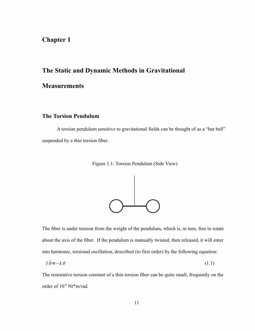
The Torsion Pendulum

A torsion pendulum sensitive to gravitational fields can be thought of as a “bar bell”

suspended by a thin torsion fiber.

Figure 1.1: Torsion Pendulum (Side View)

The fiber is under tension from the weight of the pendulum, which is, in turn, free to rotate

about the axis of the fiber. If the pendulum is manually twisted, then released, it will enter

into harmonic, torsional oscillation, described (to first order) by the following equation:

I =−k (1.1)

The restorative torsion constant of a thin torsion fiber can be quite small, frequently on the

order of 10-8 Nt*m/rad.

11

Figure 1.2: Torsion Pendulum in Oscillation (Top View)

With a torsion pendulum, there are, as described in the introduction, two techniques

for measuring a gravitational interaction: the static method, involving a stationary torsion

pendulum, and the dynamic method, involving a torsion pendulum in oscillation.

The Static Method

The “static method” is the most straightforward approach to a gravitational

experiment using a torsion pendulum. One simply measures the angular deflection of the

pendulum in the presence of a source mass. The deflection reveals the interaction strength.

Figure 1.3: Static Deflection of a Torsion Pendulum (Top View)

12

This method is limited both by the accuracy and precision to which the (very small)

deflection can be measured, and the accuracy and precision to which the torsion fiber

constant is known. In order to measure this constant, the pendulum is typically set into

torsional oscillation in the absence of ambient torques. Its oscillation period is measured,

and the torsion constant is calculated using the measured period.

In the static method, the angular displacement is typically measured using an optical

lever. Light is reflected by a mirror on the pendulum, and is observed by a position-

sensitive detector.

Figure 1.4: Optical Measurement System (Top View)

A danger in using this type of measurement (shown in Figure 1.4) is its sensitivity to

apparatus tilt, which can have quite subtle effects. If the experimental housing, within

which the torsion fiber is hung, tilts, then the pendulum will change position relative to its

immediate environment. This change in position will then result in a false reading of its

angular displacement. If this tilt correlates with the modulation of the source mass, this

error will propagate and produce a false signal. To reduce this effect, an optical system may

be built to collimate the light and focus it onto the detector. With this setup, the detector

13

remains sensitive to changes in angle, but becomes insensitive to changes in the pendulum's

displacement.

Figure 1.5: Static Pendulum Tilt (Top View)

While this setup (shown in Figure 1.5) reduces sensitivity to tilt-generated pendulum

position translation error, the apparatus remains sensitive to tilt through other mechanisms.

There are two orthogonal rotations (both shown in Figure 1.5) that do not involve a rotation

about the fiber, and both can produce a false signal.

The most obvious effect comes from a combination of a θx rotation and a misaligned

detector. This can cause the spot on the optical detector to become displaced in the z-

direction. See Figure 1.6 (a) and (b).

14

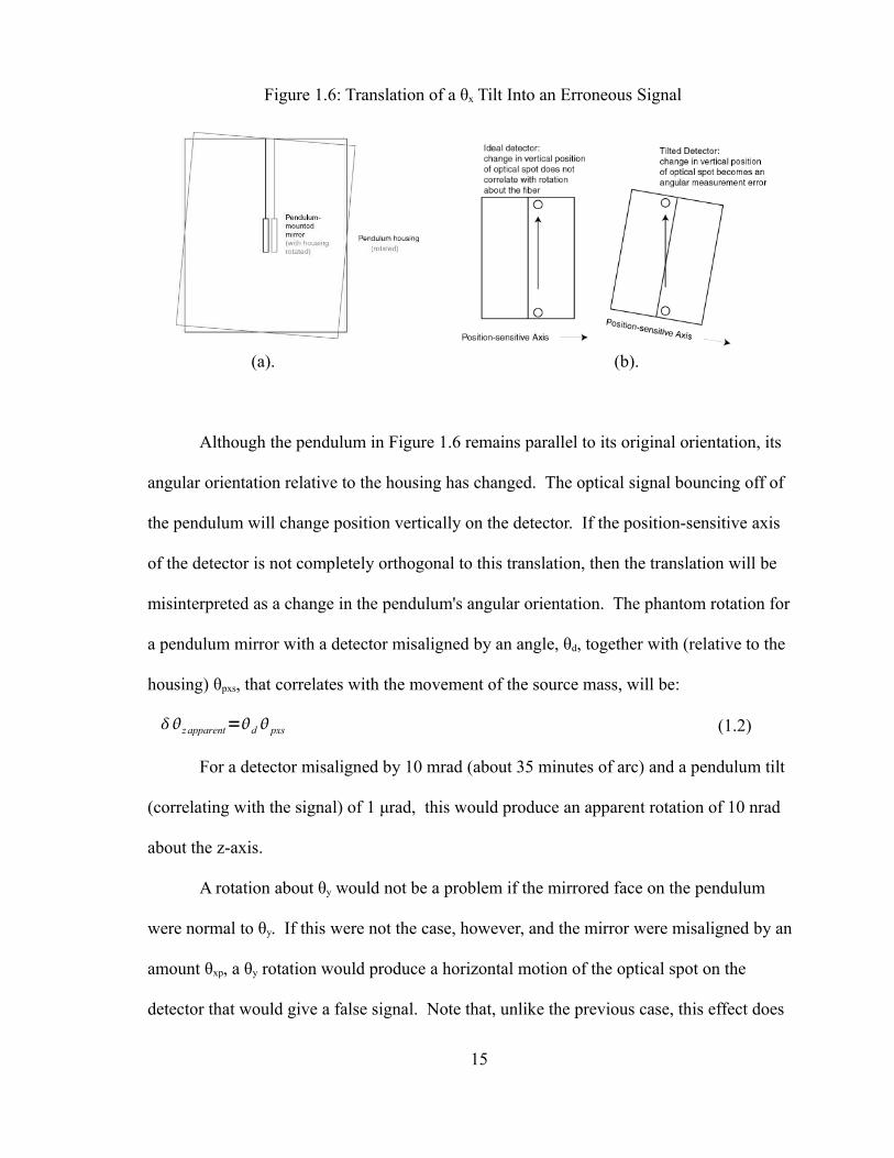
Figure 1.6: Translation of a θx Tilt Into an Erroneous Signal

(a). (b).

Although the pendulum in Figure 1.6 remains parallel to its original orientation, its

angular orientation relative to the housing has changed. The optical signal bouncing off of

the pendulum will change position vertically on the detector. If the position-sensitive axis

of the detector is not completely orthogonal to this translation, then the translation will be

misinterpreted as a change in the pendulum's angular orientation. The phantom rotation for

a pendulum mirror with a detector misaligned by an angle, θd, together with (relative to the

housing) θpxs, that correlates with the movement of the source mass, will be:

zapparent=d pxs (1.2)

For a detector misaligned by 10 mrad (about 35 minutes of arc) and a pendulum tilt

(correlating with the signal) of 1 μrad, this would produce an apparent rotation of 10 nrad

about the z-axis.

A rotation about θy would not be a problem if the mirrored face on the pendulum

were normal to θy. If this were not the case, however, and the mirror were misaligned by an

amount θxp, a θy rotation would produce a horizontal motion of the optical spot on the

detector that would give a false signal. Note that, unlike the previous case, this effect does

15

not depend upon a misaligned detector. For a pendulum misaligned (about the x-axis) by

an angle θpx, and a tilt of the pendulum, correlated with the source mass, of θpys:

z apparent=px pys (1.3)

A pendulum tilted 10 mrad about the x-axis, coupled to a signal-correlated tilt of

1μrad about the y-axis, for example, would produce an apparent rotation about the z-axis of

10 nrad.

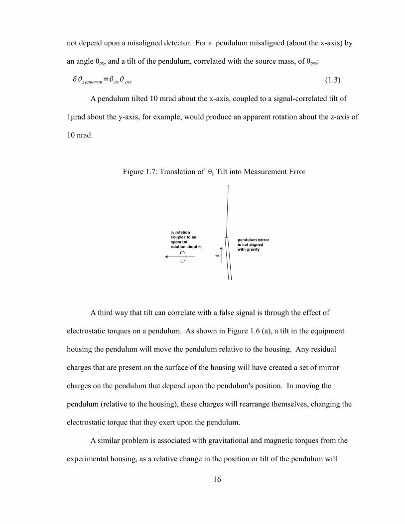
Figure 1.7: Translation of θy Tilt into Measurement Error

A third way that tilt can correlate with a false signal is through the effect of

electrostatic torques on a pendulum. As shown in Figure 1.6 (a), a tilt in the equipment

housing the pendulum will move the pendulum relative to the housing. Any residual

charges that are present on the surface of the housing will have created a set of mirror

charges on the pendulum that depend upon the pendulum's position. In moving the

pendulum (relative to the housing), these charges will rearrange themselves, changing the

electrostatic torque that they exert upon the pendulum.

A similar problem is associated with gravitational and magnetic torques from the

experimental housing, as a relative change in the position or tilt of the pendulum will

16

change the magnitude of these torques. All of the effects described above can create

systematic measurement errors if correlated with a modulation of the gravitational source

mass. Even if uncorrelated, these effects can degrade the precision of an experiment by

contributing to background noise.

Variations on the static method are also sensitive to tilt error. In an “electrostatic

compensation” measurement, an electrostatic torque is applied to the (grounded) pendulum.

An optical feedback loop ensures that the pendulum does not move, relative to the housing.

The electrostatic torques applied to the pendulum actively compensate for any external

torques during a data run. Because the feedback loop does not actually hold the pendulum

in one position, but instead holds a reflected optical spot in one position, it is subject to the

same errors as a traditional static experiment.

In another variation of the static method, “inertial compensation,” no compensating

torque is applied. Instead, the pendulum hangs within its housing, on a rotating platform.

The platform, in turn, is made to accelerate or decelerate, at a rate such that the torsional

angle between the pendulum and its housing does not vary. This acceleration is controlled

by a feedback loop, using the optical lever as a reference. When the source masses are in

place on the housing, both the pendulum and the housing will begin to rotate at constant

acceleration, and by measuring that acceleration, the strength of the gravitational torque is

inferred. This setup is less sensitive to tilt than a standard deflection experiment, because

any tilt or ambient torque would have to rotate with the pendulum in order to have a

systematic effect on the measurement.

An inertial compensation experiment has its own unique difficulties. For instance, if

the pendulum is not perfectly centered, a rotation of the apparatus will displace the

17

pendulum relative to the apparatus, causing it to swing. Accelerating apparatus rotation will

eventually cause the pendulum to become displaced (relative to the apparatus frame) as a

result of centrifugal forces.

The Dynamic Method

As discussed previously, in a “dynamic,” or “time of swing” measurement, the

pendulum oscillates while data is taken. A gravitational torque is applied, and this changes

the frequency of oscillation. This change in the frequency of oscillation indicates the

interaction strength.

Figure 1.8: Dynamic Method (Top View)

a. No Source Mass b. Source mass c. Source mass2=0

2 lowers oscillation raises oscillation frequency for frequency for small A small A 2=0

2−2 2=022

If the net average torque from the source mass (over one period) acts to restore the

pendulum to its equilibrium position, then the frequency is increased, as though the fiber's

restorative torque had increased. On the other hand, if the net average torque acts to resist a

18

return to equilibrium by the pendulum, then the frequency is decreased, as though the fiber

were slightly less stiff.

Determination of the oscillation period in the dynamic method is relatively

straightforward. As with the static method, an optical lever measures the angle of the

pendulum. As the pendulum rotates and the imaged, reflected beam crosses a particular

position on a detector, the time is recorded (I will call this event a “crossing” or “zero

crossing”). The intervals between this crossing and subsequent crossings are used to

determine the oscillation period.

Tilt in the Dynamic Method

Unlike the static method, the dynamic method is relatively insensitive to tilt. This is

because a tilt-induced mismeasurement of the pendulum's angle should not affect a

measurement of the interval between crossings.

Any tilt of the housing can only affect the crossing time by a fixed amount, Δt.

Because this will affect all subsequent crossings equally, it will not affect the measured

frequency during a time interval during which the tilt does not change. It would only shift

the zero crossing by a contstant amount for all zero crossings, and any constant-time offset

will have no effect. Thus, even if the apparatus or pendulum has a tilt that correlates with

the source mass position, the period measurement will not be affected.

A Variation of the Dynamic Method : The Second Harmonic method

As described in Appendix C, local perturbative gravitational fields not only change

the frequency of oscillation of the oscillator, they also create higher frequency harmonics in

19

the pendulum's motion. These harmonics will change sign with a modulation of the source

mass. A gravitational method could be set up to detect these harmonics, by measuring θ(t)

at several points during each cycle, using a fitting routine to extract the harmonics, and

correlating the signal to that portion of the harmonics that modulate with the source mass.

As of the date of publication of this dissertation, the author is not aware of any measurement

of G having been performed using this method.

20

Chapter 2

Principles of the UCI G Measurement Approach

While every torsion pendulum gravitational experiment will have certain features in

common, there are a number of key features of this particular measurement that are either

unique among gravitational experiments, or else uncommon enough to merit mention and

explanation. These include:

• Ring-shaped field source masses

• A flat, thin pendulum

• Several large torsional oscillation amplitudes

• Variation in types of fibers during the experiment

• Cryogenic temperatures

Ring-shaped field source masses

Placed at a particular separation distance, the ring-shaped source masses null all 3rd,

4th, and 5th spatial derivatives of their gravitational potential field at the midpoint of the

rings' common axis. The result is that the source masses exert a torque on a pendulum

placed near the rings' spatial midpoint which is extremely insensitive to error in the

pendulum's position. This is explored further in Chapter 3.

21

Flat, thin pendulum

A flat, thin pendulum in the presence of the field generated by this ring configuration

has a torsional oscillation frequency which is extremely insensitive to the pendulum's

dimensions. Both this feature and the ring-shaped field source masses serve to greatly ease

the demands for precision metrology. See chapter 3.

Large Torsion Amplitude

The torque from static field interactions can be expressed as a Fourier series of

component torques that are periodic under a full rotation:

=−∑mmcos m−∑

mm sinm (2.1)

The minus signs are used to keep this equation consistent with the formalism discussed in

Appendix C. For the UCI G experiment, these torques are zero by design through m=5,

except for the component,

s=−∑m2 sin2 (2.2)

This torque is deliberately nonzero, and its effect on the frequency is the quantity

measured in the UCI G experiment.

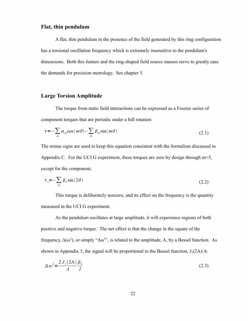
As the pendulum oscillates at large amplitude, it will experience regions of both

positive and negative torque. The net effect is that the change in the square of the

frequency, Δ(ω2), or simply “Δω2”, is related to the amplitude, A, by a Bessel function. As

shown in Appendix 3, the signal will be proportional to the Bessel function, J1(2A)/A:

2=2 J 12A

A2

I(2.3)

22

Figure 2.1: Δω2 (Arbitrary Scale) vs. A (Radians) for the UCI Experiment

2 4 6 8 10

A

2

While the magnitude of the signal strength tends to decrease with increasing

amplitude, operating at the extrema of the function yields good signal to noise ratio while

ensuring minimal sensitivity to error in amplitude determination. See chapter 6 for more

details. In addition, measurement of G based on operation at different amplitudes permits

an important check of anelastic effects and other error sources.

Different Fiber Types

This provides another important check of fiber-dependent anelastic effects and other

error sources. As described in further in chapter 4, the UCI G experiment uses Al 5056

fibers, heat treated CuBe fibers, and CuBe fibers as drawn.

Cryogenic Operation

The cryogenic aspects of the UCI experiment will help the measurement in several

ways. Thermal noise torque, for instance, is proportional to k BT /Q , where Q is the

mechanical quality factor of the oscillation. The experiment benefits here in two ways from

23

the cryogenic temperatures. Directly, the temperature itself is lower. Indirectly, the internal

friction of the fiber is greatly reduced at low temperature, resulting in a much higher Q.

In addition, thermal control is better, as the experiment is submerged in a bath of

liquid helium, fixing the temperature of the walls of the vacuum chamber. In addition, the

materials used to fabricate the experiment are less sensitive to changes in temperature, this

close to absolute zero. Variation of fiber torsion constant with temperature, and consequent

variation in torsional frequency is an important source of noise in the dynamic method; thus,

the reduced temperature sensitivity, coupled with the ability to maintain a highly constant

temperature are of great benefit.

Furthermore, at low temperatures, cheap materials (such as the lead foil used in the

UCI G experiment) become superconductive, so that ambient magnetic fields passing

through a lead envelope will become “pinned,” shielding the pendulum from ambient

magnetic field modulation.

Lastly, the low temperature helps to achieve an extremely high vacuum. First,

materials will outgas much less at low temperatures, and second, any gases that do touch a

cold surface are much more likely to stick to it, rather than bounce off. This helps to

achieve very high vacuum in the region of the pendulum. Pressures as low as 10-7 mBar

were measured at the room temperature portion of the vacuum chamber while the vacuum

can was immersed in liquid helium, and the pressure in the low temperature region should

have been much lower than this, although we did not have a device capable of measuring

the pressure at such low temperatures.

24

On the down side, cryogenic equipment can be difficult to deal with. Opening up the

experiment to fix problems becomes very time consuming, and many electronic devices do

not function well at low temperatures.

Throughout any G experiment, it is vital to keep in mind, at all times, that the

pendulum and source masses are not isolated from the rest of the universe, but are housed

with, and measured, timed, modulated, and regulated by equipment that may itself introduce

errors. These error sources include temperature variation, tilt, vibration, electrostatic

interactions, magnetic interactions, wire cross-talk, digitization errors, computer program

errors, etc. Some of these error sources are beyond the scope of this dissertation, but most

are fully capable of introducing systematic errors sufficient to embarrass even an extremely

capable scientist.

25

Chapter 3

Motivation for the Design of the Source Mass Rings and

Pendulum

In the UCI experiment, a multipole formalism is used to extract G from the

measured frequency shift produced by moving the source mass rings. Here, we briefly

outline that formalism; details will be presented in chapter 6 and Appendix C.

The combined torque experienced by the pendulum from the restoring torque from

an ideal torsion fiber plus the gravitational interaction of the pendulum with its environment

may be expressed:

=−k −ℜ∑l=1

∞

∑m=−l

l

imqlm a lme−i m (3.1)

where k is the fiber's torsion constant and the qlm and alm are respectively pendulum mass

multipole moments and field multipole moments, defined in Appendix C. The frequency

when the pendulum is placed in torsional oscillation is given by

2≃02[1 2

A∑m=1

∞

J 1m Am

k ] (3.2)

where ω02 = k/I, I is the pendulum's moment of inertia, A is the torsional oscillation

amplitude, and βm is given by:

26

m=−2mℜ∑l=m

∞

q lma lm (3.3)

Equation 2 is accurate to first order in the ratio β2/k.

The symmetry of the pendulum is such that βm = 0 for odd m. The field moments alm

and hence the βm depend on the position of the source masses. When the ring field mass

system is rotated about the pendulum's fiber axis by 90 degrees, β2 and β6 retain the same

magnitude but reverse their sign, while β4 is unchanged. Defining Δsω2 to be the change in

the square of the torsional frequency when the ring source mass system is rotated by 90

degrees, we then find:

s2= 4

I A [2 J 12A 6 J 16A O 8 ] (3.4)

As the alm, and hence βm, are each proportional to G, it is clear that equation 4 may be

expressed in the form:

s2=C A×G (3.5)

so that G may be found:

G=s

2

C A(3.6)

For the pendulum and source mass parameters of the UCI G measurement, the term

proportional to β6 in equation 4 represents a correction of only a few ppm to the dominant

term proportional to β2. Thus in much of this thesis, the emphasis will be on error sources in

determining β2, and the signal frequency shift will be normally approximated as:

s2= 4

I A2 J 12A (3.7)

The source masses and pendulum used in the UCI G measurement have a variety of

geometric properties designed to minimize sensitivity to error in mass and dimensional

27

metrology. The pendulum is thin and square, while the source mass consists of two rings,

placed symmetrically on either side of the pendulum at a particular calculated separation.

Ring Design

The UCI G experiment uses two copper rings as a source mass, designed to give a

well-defined gravitational signal in the form of a change of frequency of oscillation.

A careful choice of ring geometry and separation can generate a gravitational

potential whose spatial derivatives of order 1 and 3-5 vanish at a point midway between the

rings. The remaining low order derivatives correspond to the gradient of g – a field

derivative that couples to the quadrupole moment of the pendulum. The vanishing of the

next three derivatives means that the gradient of g is nearly constant over a large volume.

This makes the coupling of the source mass rings to the pendulum becomes extremely

insensitive to error in the rings' placement.

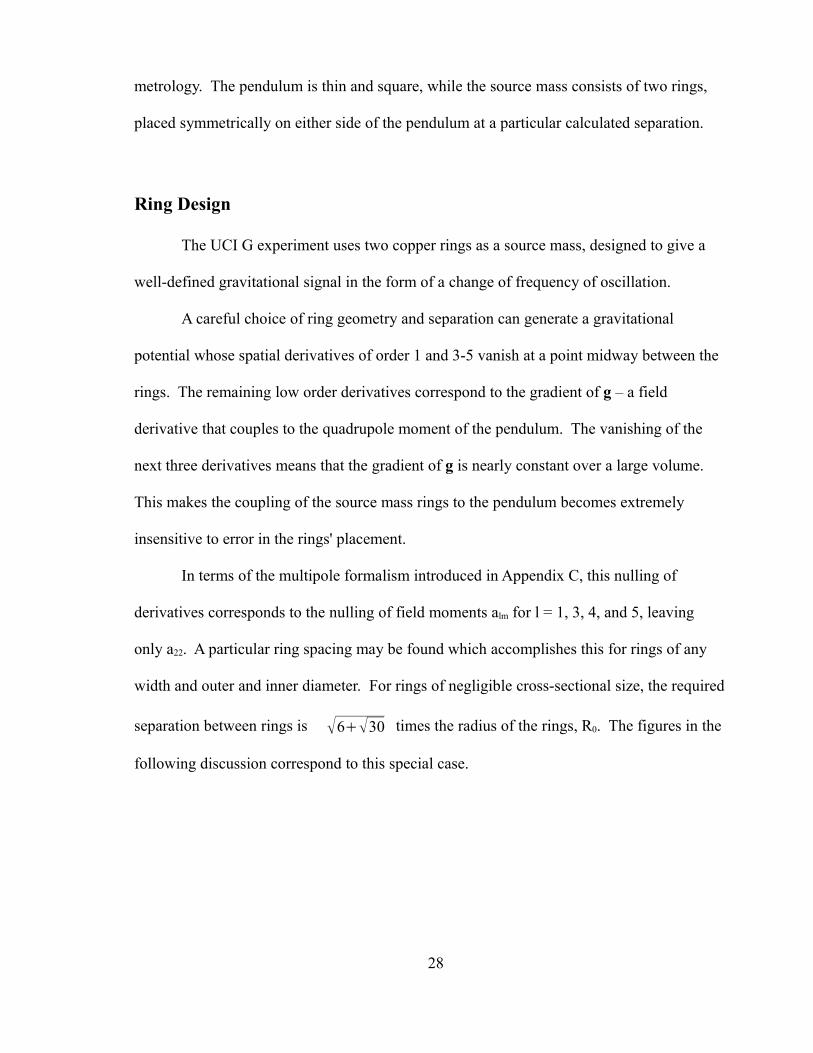
In terms of the multipole formalism introduced in Appendix C, this nulling of

derivatives corresponds to the nulling of field moments alm for l = 1, 3, 4, and 5, leaving

only a22. A particular ring spacing may be found which accomplishes this for rings of any

width and outer and inner diameter. For rings of negligible cross-sectional size, the required

separation between rings is 630 times the radius of the rings, R0. The figures in the

following discussion correspond to this special case.

28

Figure 3.1: Model of Thin Rings

Source Masses

A convenient method to get a sense of the symmetry is to examine the gravitational

potential along the axis of symmetry of the rings. This allows for a more intuitive

exploration of the geometry than an alm formulation might. Because the desired ring

separation is proportional to the rings' radius, all of the following graphs will have an x-axis

that is denominated in ratios to that radius.

Figure 3.2: Gravitational Potential of an Idealized

Coaxial Two-Ring System, Along the Axis of Symmetry

(arbitrary vertical axis)

4 2 2 4

x

R0

Gravitational Potential

The gravitational potential cannot be directly measured, and the gravitational g field

29

of the rings is zero at the midpoint (by symmetry). The leading measurable non-zero term is

therefore the derivative of the field vector g, and it is this term that is proportional to the

experimental signal. The reason why is that we are measuring a quadrupole torque. A

dipole pendulum moment would respond to the gravitational g field. However, an

important feature of any torsion pendulum is that it necessarily has no horizontal mass

dipole moment relative to its suspension axis. Hence, only g field derivatives contribute to

the torque it experiences.

Figure 3.3: ∂ g x

∂ x=−∂2

∂ x2 of an Idealized

Coaxial Two-Ring System, Along the Axis of Symmetry

(arbitrary vertical axis)

4 2 2 4

x

R0

ddx of Gravitational Field

Directly at the origin, the third, fourth, and fifth partial derivatives of the

gravitational potential are all equal to zero. Odd derivatives are zero by symmetry, and the

fourth derivative is nulled by the choice of ring spacing. This symmetry doesn't only apply

to the x-coordinate. All derivatives of the potential field, of order 3 through 5, can be shown

to vanish at the midpoint between the rings with the proper separation.

First, it should be realized that all y- and z- derivatives are interchangeable at the

30

origin due to symmetry, to all orders. Working from the fact that the Laplacian of the field

is zero anywhere except on the one-dimensional rings, ie,

∂2∂ x2

∂2∂ y2

∂2∂ z2 =0 (3.8)

we can use the the symmetry in y and z to show:

∂2∂ x2 =−2 ∂

2∂ y2 =−2 ∂

2∂ z2 at the origin (3.9)

Consider the Φxx and Φyy terms from equation 9, and take their second derivative with

respect to x.

∂4∂ x 4 =−2

∂2∂2∂ y2 ∂ x2 =−2

∂2 ∂2∂ x2 ∂ y2 at the origin

(3.10)

Combining the equations 10 and 9,

∂4∂ x 4 =−2

∂2∂2∂ y2 ∂ x2 =−2

∂2 ∂2∂ x2 ∂ y2 =4 ∂

4∂ y4 at the origin

(3.11)

So not only is the fourth derivative of the field with respect to x equal to zero (by

construction), but so is the fourth derivative of the potential field Φ with respect to y. By

symmetry, this must be true of z as well, and any fourth derivative of the field constructed

by some combination of x-, y-, and z-derivatives. By a similar technique, it can be shown

that any odd derivatives of Φ (in any combination) are zero as well, as a result of the three

components of the force being zero at the origin (due to symmetry).

Only at the sixth derivative of the field do we see a nonzero value. Because the

gravitational interaction with the pendulum is proportional to the derivative of the vector

field g, and this derivative is nearly constant over a large volume, the gravitational

31

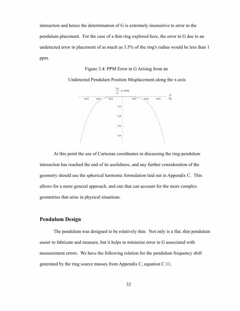
interaction and hence the determination of G is extremely insensitive to error in the

pendulum placement. For the case of a thin ring explored here, the error in G due to an

undetected error in placement of as much as 3.5% of the ring's radius would be less than 1

ppm.

Figure 3.4: PPM Error in G Arising from an

Undetected Pendulum Position Misplacement along the x-axis

0.03 0.02 0.01 0.01 0.02 0.03

x

R0

0.8

0.6

0.4

0.2

G

G, in PPM

At this point the use of Cartesian coordinates in discussing the ring-pendulum

interaction has reached the end of its usefulness, and any further consideration of the

geometry should use the spherical harmonic formulation laid out in Appendix C. This

allows for a more general approach, and one that can account for the more complex

geometries that arise in physical situations.

Pendulum Design

The pendulum was designed to be relatively thin. Not only is a flat, thin pendulum

easier to fabricate and measure, but it helps to minimize error in G associated with

measurement errors. We have the following relation for the pendulum frequency shift

generated by the ring source masses from Appendix C, equation C.11,

32

2=∑m=1

∞

2m

IJ 1mA

A (3.12)

And, from Appendix C, equation C.30,

m=−∑l=m

∞

2mℜq lm alm (3.13)

where the a's represent the gravitational field of the source mass, and the q's represent the

responsiveness of the test mass. If the gravitational source masses are fabricated and

oriented in such a way that the signal is dominated by a real a22 term, equation 12 can be

expressed as

2=−8ℜ q22

I a22

J 12AA (3.14)

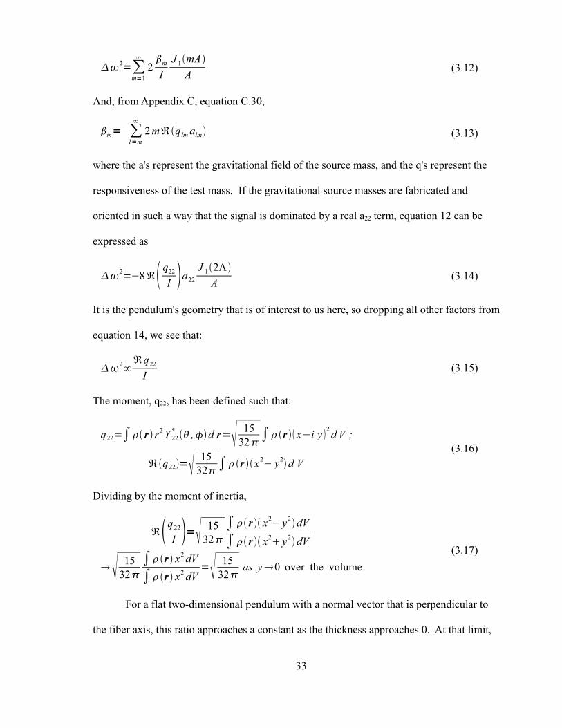
It is the pendulum's geometry that is of interest to us here, so dropping all other factors from

equation 14, we see that:

2∝ℜq22

I(3.15)

The moment, q22, has been defined such that:

q22=∫ r r2 Y 22* ,d r= 15

32∫r x−i y 2 d V ;

ℜq22= 1532∫r x2− y2d V

(3.16)

Dividing by the moment of inertia,

ℜq22

I = 1532

∫ r x2− y2dV

∫ r x2 y2dV

1532

∫r x2 dV

∫r x2 dV= 15

32as y0 over the volume

(3.17)

For a flat two-dimensional pendulum with a normal vector that is perpendicular to

the fiber axis, this ratio approaches a constant as the thickness approaches 0. At that limit,

33

any geometry will suffice. A two-dimensional pendulum shaped like Figure 3.5 (b) will

experience the same change in frequency squared (Δω2) in the presence of a uniform

gravitational field gradient as any other flat two-dimensional shape would.

Figure 3.5: Pendulum

(a) (b) G Pendulum Arbitrary 2-D Pendulum

In addition to making the pendulum flat and thin, a deliberate choice of width-height

ratio can also have an important effect upon the pendulum's behavior. While any geometry

will give the same frequency shift in the presence of a gravitational potential of constant

gradient, not all pendulums will respond equally to fields with non-zero higher derivatives.

Another geometric choice to consider is a pendulum designed to null the pendulum's

q42 moment. This was the approach taken by Gundlach et al [7]. Expressed in Cartesian

coordinates,

q42=−38 5

2∫r x−i y 2x2 y2−6 z2dV (3.18)

For a geometrically perfect, rectangular pendulum, for example, this moment is zero

when the dimensions obey the following relation:

34

height= 310∗thickness2width2 (3.19)

For a perfectly thin pendulum, this means that the height is about 55% of the width. This

will complement any nulling of the a42 produced by a careful choice of source mass

geometry, described above.

Alternatively, one could choose to null the pendulum's q62 moment through a similar

method, resulting in a choice of pendulum height that obeys one of the following relations:

height= thickness 2

2width2

2±13 thickness434 thickness2 width213 width4

47(3.9)

For a thin pendulum, this means that the height is approximately either 92% or 40% of the

width.

For a well-designed double ring shaped source mass, the q62a62 term is likely to be

the leading nonzero quadrupole correction to the q22 a22 term, so this geometry might be

favorable for some G experiments.

35

Chapter 4

The Experimental Apparatus

This chapter describes the key components of the experimental apparatus used in the

UC Irvine measurement of G.

36

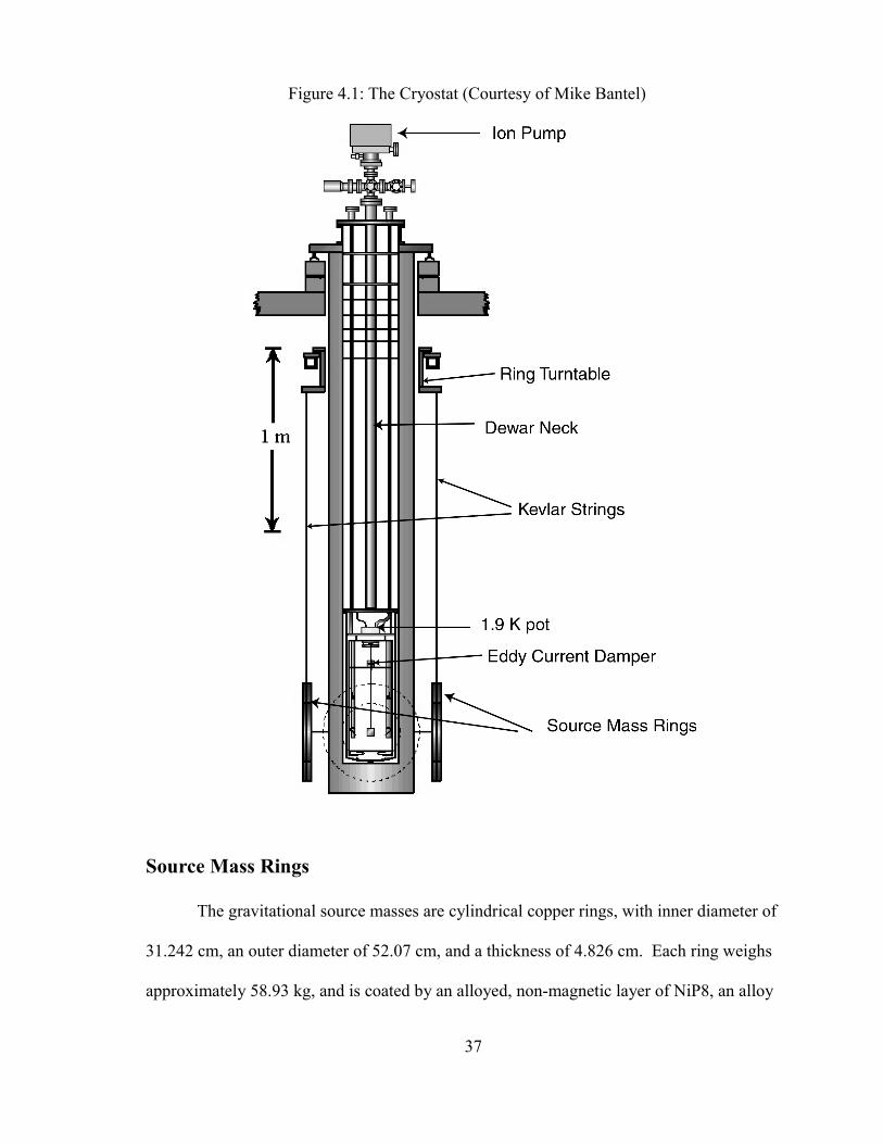
Figure 4.1: The Cryostat (Courtesy of Mike Bantel)

Source Mass Rings

The gravitational source masses are cylindrical copper rings, with inner diameter of

31.242 cm, an outer diameter of 52.07 cm, and a thickness of 4.826 cm. Each ring weighs

approximately 58.93 kg, and is coated by an alloyed, non-magnetic layer of NiP8, an alloy

37

of nickel and approximately 9% phosphorous, ~7.5 μm thick (the density is well matched to

that of the copper, so the precise thickness is irrelevant; a 50% discrepancy in the thickness

will give only a 0.5 ppm change in G, while the thickness is, in fact, known to about 25%).

The rings are tapered by about 20 μm (ring 1) or 12 μm (ring 2), and both are slightly

thicker at the outer diameter than the inner diameter. The total correction δG/G from this

tapering is approximately 24 ppm. Density varied throughout the ring's diameter by

approximately 15 ppm. Assuming that this variation is linear from one side of the ring to

another, it would give a δG/G of approximately 0.2 ppm (with small variations that depend

upon the ring's orientation). Due to symmetry, radial density variations (those that do not

vary with azimuthal angle) do not produce first-order changes in ring field moments, and

can be ignored. The inner and outer ring edges have chamfers of projected width 0.62mm.

Figure 4.2: Copper Source Mass Ring (one)

The rings are suspended 1.87 meters below the bottom of the turntable by Kevlar

string of linear density 1.4 g/mm, which wraps around the bottom of each ring, and back up

to a mount, constrained by an azimuthal groove in the outside of each ring 1.25 mm wide

and 1.25 mm deep. The two Kevlar string mounts for each ring are located approximately

17.5 cm apart. In order to maintain the separation between the two rings, two rods of fused

38

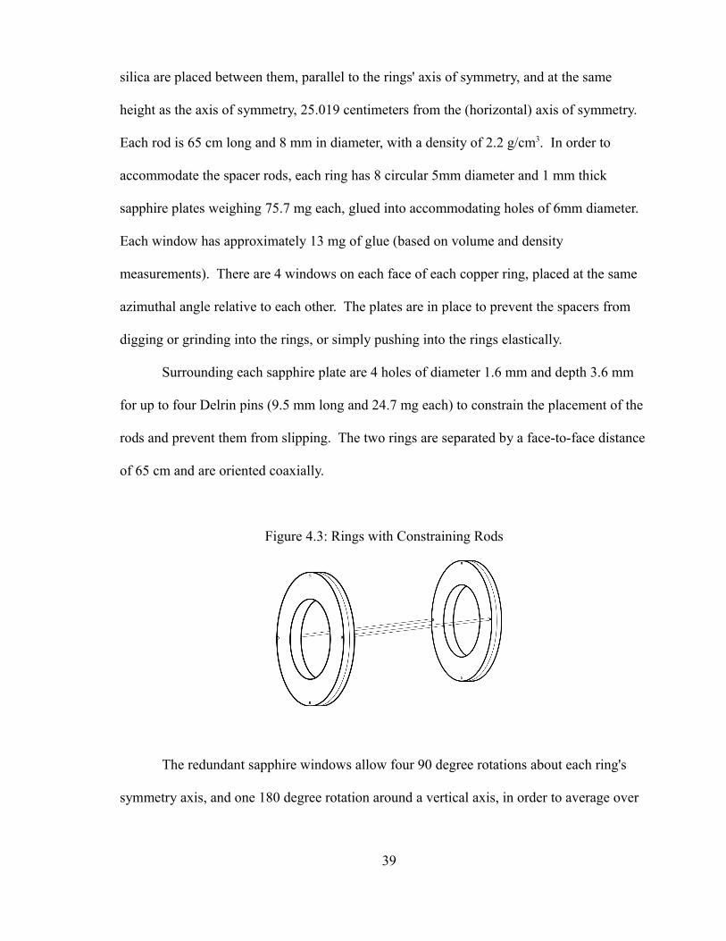
silica are placed between them, parallel to the rings' axis of symmetry, and at the same

height as the axis of symmetry, 25.019 centimeters from the (horizontal) axis of symmetry.

Each rod is 65 cm long and 8 mm in diameter, with a density of 2.2 g/cm3. In order to

accommodate the spacer rods, each ring has 8 circular 5mm diameter and 1 mm thick

sapphire plates weighing 75.7 mg each, glued into accommodating holes of 6mm diameter.

Each window has approximately 13 mg of glue (based on volume and density

measurements). There are 4 windows on each face of each copper ring, placed at the same

azimuthal angle relative to each other. The plates are in place to prevent the spacers from

digging or grinding into the rings, or simply pushing into the rings elastically.

Surrounding each sapphire plate are 4 holes of diameter 1.6 mm and depth 3.6 mm

for up to four Delrin pins (9.5 mm long and 24.7 mg each) to constrain the placement of the

rods and prevent them from slipping. The two rings are separated by a face-to-face distance

of 65 cm and are oriented coaxially.

Figure 4.3: Rings with Constraining Rods

The redundant sapphire windows allow four 90 degree rotations about each ring's

symmetry axis, and one 180 degree rotation around a vertical axis, in order to average over

39

mass distribution asymmetries using successive data sets taken with different ring

orientations.

In order to measure the temperature of each ring, platinum thermometers were

placed in each ring with grease, for a total mass of 80 mg for the platinum thermometer plus

grease. They were affixed in a 2mm diameter hole 6.35 mm deep on the outside rim of each

ring, 45 degrees azimuthally from the sapphire windows.

A turntable allowed for changes in the ring height and adjustment of the ring

orientations. The ring modulation software was carefully calibrated to ease the rings into

position quickly (roughly 1-2 minutes per transport) and with minimal swinging, although

there was always some residual ring oscillation remaining. A laser beam reflected by a

small mirror mounted on one of the rings to a two-axis position sensor served to sense

residual swing motion of the rings following their periodic repositioning. The entire mirror

and mount assembly weighed 261 mg, with a center of mass approximately 3.5 mm from

the outer edge of the ring. The reflected laser beam was used by the software to control

small rotations of the turntable from which the rings were suspended in order to damp the

swing motion. Ring position consistency was maintained between successive ring

modulations with the data from a separate set of lasers reflected off of mirrors on the

turntable.

Had this action not been taken, the swinging rings would have systematically applied

a smaller than expected net torque on the pendulum. As shown in appendix C, a relative

rotation φ between the pendulum and the source mass results in a sinusoidal change in the

torque; for a β2-dominated interaction, this goes as Cos(2φ) or, for small rotations,

40

d(log β2) = - 2 φ2. A pair of rings swinging in this fashion would require a time average of

the torques applied to the pendulum.

The Pendulum

The pendulum used in the G experiment is approximately a square, 40 mm by 40

mm, and 3 mm thick, weighing 10.9 g.

The pendulum is composed of fused silica (Corning 7989-OAA, density 2.2006

g/cm3), coated with a layer of aluminum (100 nm ± 10nm) + SiO2 (27nm ± 2.7 nm). The

2004 and 2006 data added a layer of chromium (5 nm) plus a layer of gold ( 200 nm ± 20

nm). At the top of the pendulum is a hole, 1mm in diameter and a depth of 4 mm, into

which is glued a brass screw weighing 42 mg ± 3 mg. The glue used was on the order of 1.4

mg of Stycast 1266. Each edge of the pendulum had a chamfer, approximately 0.44 mm

wide.

Figure 4.4: The UCI G Pendulum

As described in chapter 3, the pendulum is designed to be as thin as is practical in

order to minimize the sensitivity to machining and metrology errors of the ratio of the signal

41

sensitivity to the moment of inertia, q22/I. Its two-fold symmetry nulls the value of the

Newtonian moments, qlm, for odd m.

Unfortunately, one of the pendula, during a gold coating process, was damaged. A

chip of fused silica (and the accompanying coating) broke off during the coating process,

and the repaired pendulum was later used in the 2004 data runs.

Fibers

The UCI G experiment used three different fibers in order to procure a range of data

under different values of Q, with different anharmonic torque strengths, and for different

materials. The first type of fiber was a copper beryllium (CuBe) fiber. The second type was

a CuBe fiber that was then heat treated at 320 C for approximately 8 hours, then cooled at a

rate of 30 C per hour to room temperature.

The fibers varied in length but were approximately 25 cm long. At each end, the

fiber was glued into a mount consisting of a hand-cut length of aluminum tubing

(approximately 2 cm long) using Stycast 1266 epoxy. For further details, see Bantel [18]

Eddy Current Swing Mode Damping System

In order to quickly damp swing mode oscillations of the pendulum, the apparatus

was built with an eddy current damping system, with magnetic fields bridging the vacuum

gap between the top and bottom portions of the device. The damper uses a two-stage

pendulum suspension, with a stiff upper fiber that will flex if the G pendulum is swinging

but will not allow significant rotation at expected amplitudes.

42

Figure 4.5 Cross Section of an Azimuthally Symmetric

Swing Mode Eddy Current Damping Device

In addition to swing modes, the pendulum has an oscillatory degree of freedom in

which it may “bounce” up and down, stretching its torsion fiber. Such oscillation can

couple nonlinearly into a torque on the pendulum which could be a source of systematic

bias. To damp this bounce mode, we experimented with the modified eddy current damping

system shown in Figure 6. A spring was added to allow the eddy current damping disk to

oscillate vertically, and the magnet shape was altered.

43

Figure 4.6: Swing and Bounce Mode Eddy Current Damper

This system was tested with a 240 gram pendulum designed for future planned

experiments, but failed to reduce observed noise levels.

Vacuum System

The stainless steel vacuum can has an OD of 27.3 cm, an ID of 26.6 cm, and 78.7 cm

of full ID (with rounded bottom). The vacuum chamber has a long neck, 5.1 cm in diameter

and 205 cm long from the top of the vacuum can to the top plate of the insert. During data

runs, the helium level is somewhere above the top of the vacuum can but below the lowest

of seven baffles, approximately 1.2 meters above.

44

The vacuum in the region of the G pendulum is achieved through a multi-stage

process. After the vacuum chamber is sealed, it is pumped down using a turbo pump

(Varian Turbo-V70) backed by a diaphragm pump (Varian VS102). The turbo

pump/diaphragm pump combination was chosen in order to avoid oil migration into the

vacuum chamber.

When the pressure drops low enough, (~10-5 mbar), an Varian triode 20 l/s ion pump

is engaged to bring the pressure down to approximately 10-6 mbar. When the dewar is filled

with liquid helium, the pressure drops further through molecular adhesion to any cold

surface. This effect is exploited with several cubic centimeters of activated charcoal in the

vacuum chamber. After being exposed to atmosphere, this charcoal was heated during its

initial exposure to vacuum in order for it to outgas.

At the location of the ion pump (at the top of the apparatus and at room

temperature), the cryopumping is able to generate a vacuum on the order of 10-7 mbar. This

room-temperature pressure is likely to be orders of magnitude larger than the pressure at the

location of the pendulum.

During the 2000, 2002, and 2004 data runs, the ion pump was usually on while data

was being taken. During the 2006 data runs, the ion pump was normally turned off, and we

relied on the activated charcoal cryopump action to maintain high vacuum for the

pendulum, as it was suspected that the ion pump contributed to a noisy readout signal

coming from the photodetector. There were also fears that the ion pump was burping gas

into the vacuum system, although this was never rigorously investigated.

45

“2K” Helium Pot

To further reduce the operating temperature of the pendulum, and to facilitate

temperature control, the cryostat includes a chamber (“2 K pot”) into which helium is drawn

from the 4.2K reservoir through a capillary tube. By pumping this pot to pressures of a few

mbar, its temperature may be reduced to 1.9K with our system (others have gotten to 1K and

below). Unfortunately, these systems typically suffer from capillary flow rate oscillations

which were later suspected of contributing to statistical noise through mechanical vibration.

Figure 4.7: The Vacuum Can of the Cryostat

(Courtesy of Mike Bantel)

Although the 2K pot was used for the entire G experiment, it will not be used in future

experiments, and we cannot recommend its use in future gravitational cryogenic torsion

pendulum experiments.

46

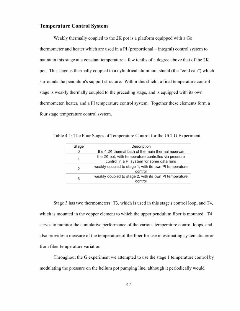
Temperature Control System

Weakly thermally coupled to the 2K pot is a platform equipped with a Ge

thermometer and heater which are used in a PI (proportional – integral) control system to

maintain this stage at a constant temperature a few tenths of a degree above that of the 2K

pot. This stage is thermally coupled to a cylindrical aluminum shield (the “cold can”) which

surrounds the pendulum's support structure. Within this shield, a final temperature control

stage is weakly thermally coupled to the preceding stage, and is equipped with its own

thermometer, heater, and a PI temperature control system. Together these elements form a

four stage temperature control system.

Table 4.1: The Four Stages of Temperature Control for the UCI G Experiment

Stage 3 has two thermometers: T3, which is used in this stage's control loop, and T4,

which is mounted in the copper element to which the upper pendulum fiber is mounted. T4

serves to monitor the cumulative performance of the various temperature control loops, and

also provides a measure of the temperature of the fiber for use in estimating systematic error

from fiber temperature variation.

Throughout the G experiment we attempted to use the stage 1 temperature control by

modulating the pressure on the helium pot pumping line, although it periodically would

47

Stage Description0 the 4.2K thermal bath of the main thermal reservoir

1

2

3

the 2K pot, with temperature controlled via pressure control in a PI system for some data runs

weakly coupled to stage 1, with its own PI temperature control

weakly coupled to stage 2, with its own PI temperature control

deviate drastically from desired temperature ranges.

In addition to heat entering the system from the control loop heaters, a fraction on

the order of 10% of the optical lever light is absorbed by the pendulum. The pendulum was

coated with a thin layer of gold after the 2004 data run in order to increase the reflectivity

(78% for the Aluminum coating, 98.7% for the gold coating).

Optics System

In order to measure the period of the pendulum, as well as the higher harmonics of

its oscillation, the pendulum is imaged using an LED at room temperature, with a fiber optic

cable to transport the light through the helium bath and into the vacuum system. The LED

used was a Honeywell HFE 4226-022 850 nm GaAlAs, mated to a 62.5 um fiber delivering

approximately 100 uW of 850 nm light at 60 mA of input current. When the light exits the

fiber optic cable, it is collimated using a 163mm focal length lens, aimed at the G pendulum

with a 45-degree aluminum coated mirror (reflectivity of ~90%), and reflected off of the G

pendulum. If the reflective surface of the G pendulum is perpendicular to the beam column,

it is reflected back towards the 45 degree mirror, and refocused by the collimating lens onto

its split photodetector. See Figure 8.

48

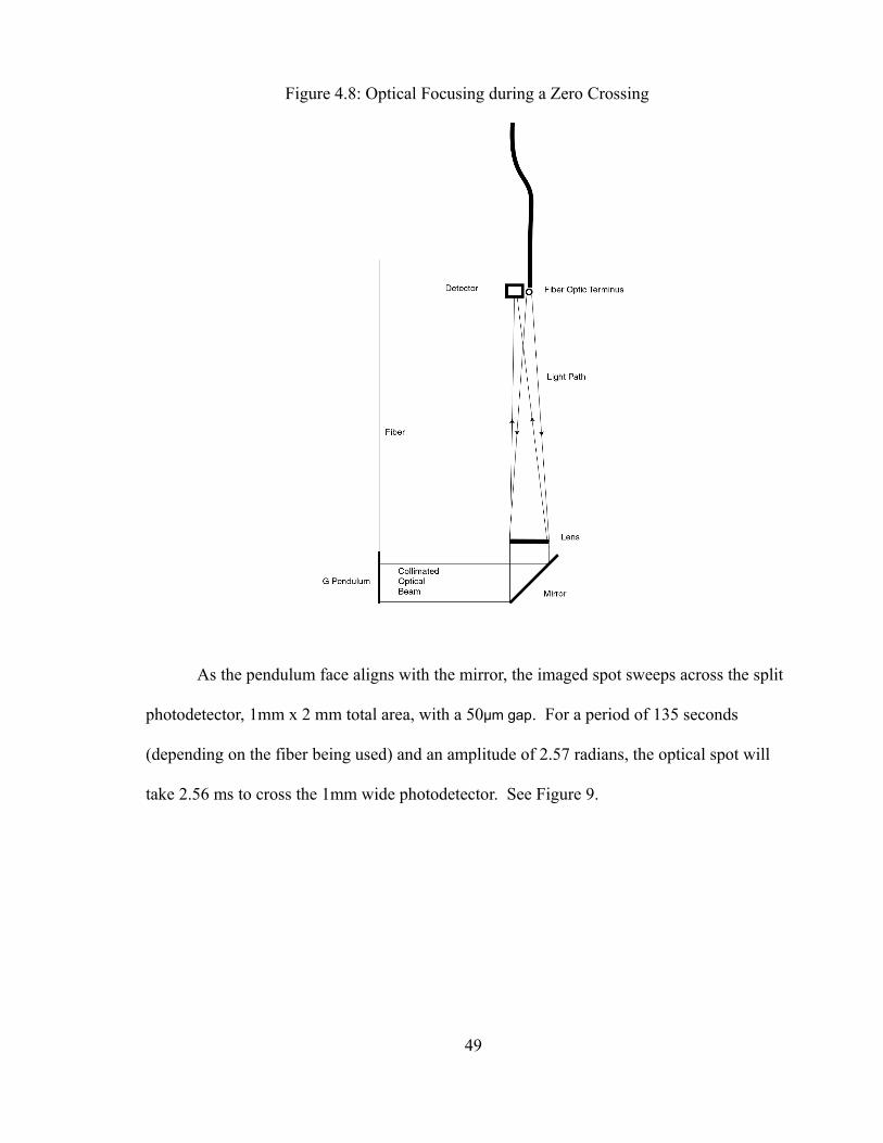
Figure 4.8: Optical Focusing during a Zero Crossing

As the pendulum face aligns with the mirror, the imaged spot sweeps across the split

photodetector, 1mm x 2 mm total area, with a 50μm gap. For a period of 135 seconds

(depending on the fiber being used) and an amplitude of 2.57 radians, the optical spot will

take 2.56 ms to cross the 1mm wide photodetector. See Figure 9.

49

Figure 4.9: Detector during a Transit

The photodetector (a CentroVision LD2A-0; peak current 10 mA, 0.54 A/W

response at 900 nm) fed current to an amplifier that typically consisted of a pair of Burr

Brown (now Texas Instruments) OPA627 op amps as “transconductance” (current-to-

voltage) amplifiers, with feedback components 1.8 Mohm in parallel with 12 pF. These go

to an INA110 differential amplifier, set for unity gain.

Each face of the photodetector generates a current that is converted into a voltage by

a resistor and summed using this setup. The moment at which the summed voltage becomes

zero is called a “zero crossing.” See Figure 10

Figure 4.10: Summed Photodetector Voltage during a “Zero Crossing”

time

V

50

Digitizations in the central region are used to construct a third-order fit, and the time

at which V=0 in this fit is recorded and used to determine the frequency of the pendulum.

In order to obtain information about the pendulum's behavior at other angles, 90 degree

aluminum mirrors (reflectivity ~ 90%) are set up in a ring around the pendulum, as shown in

Figure 11.

Figure 4.11: Placement of 4 Primary (45 degree) and Secondary (90 degree) mirrors

around the UCI G Pendulum

Although Figure 11 shows four redundant 45 degree mirrors, only one was used in G

data run.

When the collimated beam reflects off of its corresponding 45 degree mirror and

then the surface of the G pendulum, it may also reflect off of a secondary mirror. If so, it

will reflect back to the UCI G pendulum, and from there to the primary mirror, through the

51

focusing lens, to be imaged at the photodetector. This enables the measurement of specific

times when the pendulum passes through these angles, permitting greater characterization of

the pendulum's oscillation than one would achieve with only the central crossing.

Timing System

The period of the oscillating pendulum during the UCI G experiment could be as

little as approximately 100 seconds or as much as 135 seconds depending on the fiber being

used. The signal change in period when the ring system was rotated was at most 1.7 ms (for

the as-drawn CuBe fiber at 2.57 radian amplitude) and as small as 0.2 ms (for the Al5056

fiber at 7.4 radian amplitude). Thus, measuring G to 10 ppm required measuring the

oscillation periods with accuracy as great as 2 parts in 1011.

In order to achieve this level of precision, we use an HP 58503B GPS-steered crystal

controlled time base, which generated a highly accurate and stable 10 MHz sine wave

signal. This signal is converted to a square wave that is used as the digitization timebase of a

National Instruments data aquisition card (PCI-MIO-16-1: 12 bit 1.25 million

samples/second). The card uses the counter and the voltage input to feed information on

transits to the computer, which fits the data and logs the transit.

Lab Site

The experiment takes place at a location roughly 10 meters underground, in a former

NIKE missile launch site on the Hanford reservation in the desert of the eastern part of the

state of Washington. The closest publicly accessible road is approximately 5 miles from the

site, minimizing seismic noise pollution from automobiles and humans.

52

Chapter 5

Further Formalism in a Dynamic Measurement of Gravity

In chapter 3 we outlined the basic formalism for extracting a value of G from

frequency shift measurements in the UCI G experiment. That discussion assumed that the

only torques acting on the pendulum were those due to an ideal torsion fiber and an ideal

gravitational source mass. In this chapter, we extend that formalism to take into account

non-ideal fiber properties as well as external torque sources such as background

gravitational fields and magnetic fields.

In order to describe the behavior of a torsion pendulum, it is useful to subdivide the

forces (or rather, the torques) acting on the pendulum into several different categories, and

to characterize the response of the pendulum to each of these categories. The equation of

motion of the torsional pendulum will be:

I = (5.1)

where τ may be expressed:

=−{∑nk n

n∑ii , ∑

m[amcos mqbm sin m q]} (5.2)

where the first sum represents elastic torques generated by the fiber, the second sum

represents dissipative torques, and the third sum represents torques generated by pendulum

couplings to external static fields. We will consider each of these torques in turn.

53

It is convenient to think of a torsion pendulum's behavior (in the presence of only

the torque of an ideal fiber) as that of a simple harmonic oscillator:

I =−k 1 (5.3)

Solving the equation of motion, we find that (for an appropriate choice of t = 0):

0= k1

I0t =Asin 0 t

(5.4)

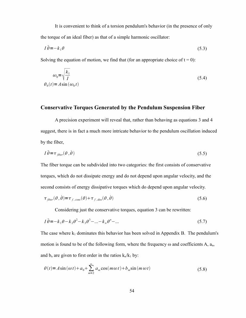
Conservative Torques Generated by the Pendulum Suspension Fiber

A precision experiment will reveal that, rather than behaving as equations 3 and 4

suggest, there is in fact a much more intricate behavior to the pendulum oscillation induced

by the fiber,

I = fiber , (5.5)

The fiber torque can be subdivided into two categories: the first consists of conservative

torques, which do not dissipate energy and do not depend upon angular velocity, and the

second consists of energy dissipative torques which do depend upon angular velocity.

fiber , = f , cons f , diss , (5.6)

Considering just the conservative torques, equation 3 can be rewritten:

I =−k 1−k 22−k 3

3−...−k nn−... (5.7)

The case where k1 dominates this behavior has been solved in Appendix B. The pendulum's

motion is found to be of the following form, where the frequency ω and coefficients A, an,

and bn are given to first order in the ratios kn/k1 by:

t =Asin t a0∑m=2

∞

am cosm t bmsin m t (5.8)

54

then the solution will take on the following values:

2

02 = ∑

n=3,5,7,. ..

∞ 12

n−1 n!

n12 !n−1

2 !An−1 k n

k 1 (5.9)

a0=− ∑n=2,4,6,. ..

∞ 12

n n!

n2 !n

2 !An k n

k1 (5.10)

am ,even= ∑n=m, m2, m4,...

∞ 1n2−1 1

2n−1

−1m2 n!

nm2 ! n−m

2 !An kn

k1 (5.11)

am ,odd=0 (5.12)

bm , even=0 (5.13)

bm, odd= ∑n=m ,m2, m4,. ..

∞ 1m2−11

2 n−1

−1m−1

2 n!

nm2 ! n−m

2 !An k n

k 1 (5.14)

The first few terms (up through m = 7) in equations 9-14 can be seen in the table at the end

of Appendix B.

During the exploration of second-order couplings (discussed in Chapter 6), these

first-order terms for k2 and k3 have been checked against the results of numerical

integrations in order to confirm their validity. Limits on computational accuracy of

approximately 10-17 seconds and 10-17 rad put an upper limit on the uncertainty in the value

given by equation 9 of less than 6 parts per billion. For this computation, k1 was set to .032

dyn cm/rad, the period was set to 135 seconds, and k2 and k3 were set to 4.8*10-5 k1.

There are a number of symmetries that appear in the oscillator's response to these

conservative torques. First, the frequency is only affected by torques of odd n. Second,

offsets are only produced by torques of even n. Third, odd n torques produce odd sine

55

harmonics, ie, a k13 term will produce harmonics of sin(13ωt), sin(11ωt), sin(9ωt), etc. This

is because the torque is an odd function of θ, and this makes the torque an odd function of t

(since we have defined that θ(0)=0 for the dominant harmonic). Similarly, the even

character of even m torques will produce even cosine harmonics.

The second group of fiber torques consists of the dissipative torques that serve to

damp the pendulum's motion. This consists of a vast parameter space of torques, only a few

of which are potentially relevant to a measurement of G. Therefore, these will be not be

described here, but a few potentially relevant cases will be described in greater detail in

chapter 6. Any torque that depends upon angular velocity, or the sign of the angular

velocity, will fit into this category.

Conservative Torques Generated by Ambient Fields

Another set of torques that act upon the torsion pendulum is caused by the ambient

static fields in the neighborhood of the pendulum. Because these torques are periodic under

a full rotation, they can be represented by a Fourier expansion:

=−∑m=1

∞

[m cos mm sin m ] (5.15)

These torques can be further subdivided into those that correlate with the motion of the

source mass, and those that do not.

As with conservative fiber nonlinearities, these field torques produce changes in

frequency, as well as harmonics. Start with the assumption that the oscillator's behavior is

dominated by a simple harmonic oscillation. The solution will be presented in the same

form as equation 8:

56

t =Asin t a0∑n=2

∞

[an cos n t bn sin n t ] (5.16)

The first-order solutions are derived in Appendix C, and the results are reproduced here:

2

02 =∑

m=1

∞

2J 1m A

Am

k 1(5.17)

a0=−∑m=0

∞

J 0m Am

k 1(5.18)

an ,even=∑m=1

∞ 2n2−1

J nmAm

k 1(5.19)

an ,odd=0 (5.20)

bn , even=0 (5.21)

bn , even=∑m=1

∞ 2n2−1

J nmA m

k 1(5.22)

As with the nonlinear fiber torques, the frequency shifts (equation 17) have been

checked during exploration of second-order couplings of various torques on the frequency

explored in chapter 6. Limits on computational accuracy of approximately 10-17 seconds

and 10-17 rad put an upper limit on the error of the first order correction given by equation 17

to less than 1 part per billion. For this computation, k1 was set to .032 dyn cm/rad, the

period was set to 135 seconds, and the field torque terms were set to 4.8*10-5 k1.

In equation 17, the fractional shift in frequency is of order of the small

dimensionless parameter βm/k1. In a dynamic measurement of G, all but one of the relevant

gravitational torque terms will be small due to a careful experimental design (see chapter 3).

That remaining torque term will dominate the signal. In the case of the UCI G experiment,

this term is β2, and the measured change in frequency is expressed as

57

2

2 s

=2 J 12A

A2

k1(5.23)

Several symmetries arise in equations 17-22. The an terms, for example arise from

αmcos(m θ) torques on the pendulum. Because

cos m =1− m22

2 !m44

4 !−... (5.24)

we would expect the an terms produced by αm to have a symmetry similar to the symmetry

produced by “even m” θm terms, which is the case. Both produce only cos(nθ) harmonics,

with even n. Both are even functions of θ and of t. Both produce a change in the offset

angle. A similar symmetry is produced by the sin(mθ) torques. The harmonics produced by

these terms are odd-integer sines, and are odd functions of θ and t. Like odd polynomial

terms of θ, these sin(mθ) terms affect the frequency of the oscillation.

Equations 17-22 form a general perturbative solution for all conservative field

interactions: electrostatic, magnetostatic, and gravitational. Each field source will

contribute its own set of αm and βm to the pendulum's motion, and any that correlate with

the motion of the source mass will contribute to the measured frequency shift.

Higher Order Effects of the Torque Perturbation Terms

Equations 17-22 describe only the first-order effect of small perturbative field

torques, and equations 9-14 are also only to first order. None of these indicate the

magnitude of any second-order (or higher) effects. These effects arise because the

pendulum's behavior deviates from that of a pure sine wave, and any alteration of the sine

wave will slightly change the perturbing effects of all torques. Unfortunately, analytic

58

methods do not lend themselves to an easy exploration of higher order frequency

perturbations. The magnitude of the second-order effects will be described in chapter 6.

59

Chapter 6

Systematic Experimental Error Sources

This chapter explores and quantifies sources of systematic error that arise in a

cryogenic torsion pendulum used to measure G with a frequency method.

Fiber

A defining feature of a torsion pendulum is that it hangs by a fiber. While low-

precision experiments can treat the pendulum as an ideal damped torsional harmonic

oscillator, this would be naïve in a high-precision experiment, where its anharmonic

behavior would bias the results. For a more complete examination of the fiber's behavior,

see Anelastic behavior of a torsion pendulum with a CuBe fiber at low temperature, and

implications for a measurement of the gravitational constant (1998), Michael Kurt Bantel's

PhD thesis [18].

A well-behaved fiber's anharmonic torques are quite small relative to its simple

harmonic torque. For the UCI G experiment, the anharmonic torques were at most five

orders of magnitude smaller than the harmonic torque.

60

Conservative Fiber Anharmonics

The simplest anharmonic torques in a fiber are terms proportional to θn, where n>1.

These can be thought of as higher order terms of a Taylor expansion of the fiber's torque as

a function of θ. They will affect the pendulum's frequency and mean angular displacement

(or “offset”), as well as generating harmonics of the fundamental sinusoidal oscillation, but

do not dissipate energy. A calculation of these effects to first order is found in Appendix B,

using the formalism laid out in Appendix A.

Anharmonic torques proportional to odd powers of θ will produce a shift in

frequency. For a torque component proportional to θ raised to an odd power, n, this

frequency shift will be proportional to a A(n-1), where A is the torsional amplitude. This can

lead to an error in G if the ring modulation produces a systematic change in the amplitude.

Consider how an error in G might arise from a torque

=−k1−k 33 (6.1)

To first order in the ratio k3/k1, this will shift the frequency by an amount,

2

2 =34

k3

k1A2 (6.2)

If the torsional amplitude A changes systematically by an amount δA when the source mass

ring positions are modulated, then there will be a systematic contribution to the total

frequency shift given by

2

2 =32

k3

k1A Asignal (6.3)

This leads to a systematic mismeasurement of G by the ratio of this value to the frequency

shift produced by the rings when they are modulated, found in Appendix C to be

approximately

61

2

2 signal

=2

k 1

4 J 12A A (6.4)

where β2 is the amplitude of the signal torque

signal=−2 sin2 (6.5)

This yields a potential error in G of

GG

=38

k 3

2

A2

J 12A Asignal (6.6)

For the amplitudes used in the experiment, this leads to the following errors:

Table 6.1: Error in G from Systematic Amplitude Excitations (δA)

during Ring Modulation due to a Torque k3 Frequency Shift

For the UCI G experiment, the value of k3/β2 is approximately -8 x 10-4 (using a

CuBe fiber as drawn), leading to a potential 1 ppm G error sensitivity due to systematic

amplitude variation of as little as 7.5 μrad (for 7.4 radian amplitude) or 5.4 mrad at 0.3

radians.

62

A (rad)

0.3 0.24

2.57 -14.6

4.21 48.9

5.81 -109

7.4 199

(dlogG /dA) / (k3/β2 )

Sensitivity to Amplitude Error

A systematic amplitude error can lead to a systematic error in G. From chapter 5,

equation 23, we define the signal measurement, s(A), to be

s A≡2

2 s

≃2 J 12A

A2

k1∝G (6.7)

(For a difference in frequency as the rings shift from one position to the other, double this

quantity) Then, using a Taylor expansion of J1(2A) at an amplitude near any A0 (defined as

any point where s is at a local extremum),

s A , A0s A0

≡s A−s A0

s A0≃−2 A−A0

2 (6.8)

The only exception is the maximum near A= 0, where the formula is

s A ,0

s A0≃− A2

2 (6.9)

Next, we can ask how much an uncertainty in the amplitude will affect a measurement of

s(A) at some amplitude near (but not at) a maximum. If (A-A0) is known to within some

accuracy, δA, then the formula is:

GG ≃[ s A , A0

s A0 ]=∂[ s A , A0

s A0 ]∂ A A≃4 A−A0 A

(6.10)

or, at 0 amplitude,

GG

≃[ s A , 0s A0 ]≃A A (6.11)

These two equations show that an experiment that takes place far from a maximum needs a

more precise measurement of the amplitude than one that takes place close to a maximum.

63

Dissipative Fiber Torques

Studies of the fibers used at UCI [17,18] and elsewhere [19] have shown that the

measured value of 1/Q as a function of amplitude for a torsion pendulum has the following

functional form:

1Q= 1

Q A=0b A (6.12)

for some value of b (for the UCI G lab, b is between 2.1*10-7 for Al and 1.5*10-6 for CuBe

fibers as drawn). We now ask what fiber behavior can account for this observed linear

dependence of 1/Q on amplitude. Because

1Q=change in energy over one period

2∗oscillator energy≡Ecycle

2 E(6.13)

and since

E≈12

k1 A2 (6.14)

we can infer that the functional form of equation 12 is caused by a torque that each cycle

dissipates energy in proportion to A3:

E= ∫cycle

A ,t , t ; t dt=constant ∗A3(6.15)

If we set our 0th order behavior to be

t =Asin t (6.16)

then we are left with the 0th order equation

E=A ∫cycle

A ,t , t ; t cos t dt=constant ∗A3(6.17)

This happens when a dissipative torque is proportional to A2, or to some function with an

integral over one period that is proportional to A2, such as θ2 or (dθ/dt)2, or some

combination. Possible combinations include:

64

A2=−k A2 A2 (6.18a)

2=−k

22 (6.18b)

2=−k 2 2 (6.18c)

A=−k A A∣∣ (6.18d)

A =−k A A (6.18e)

=−k ∣∣ (6.18f)

Note that the first four expressions require a factor,

=sign (6.19)

in order to generate nonconservative torques. Hu and Luo [19] and Peters [20] have tended

to assume the functional form of equation 18c, while Bantel and Newman [17, 18] have

modeled the amplitude-dependent Q term with the stick-slip model, represented by a

combination of equations 18a, 18b, and a non-dissipative term proportional to Aθ. Using

the method outlined in Appendix A, none of these dissipative torque expressions listed

above (equations 18a-f) will affect either the frequency or the mean angle (“offset”), though

they will produce the following “odd cosine” harmonic amplitudes (all “sine” harmonics

and “even cosine” harmonics are equal to 0):

k A2 :an=4

−1n1

2

nn2−1A2 k A2

k1, n odd (6.20a)

k 2 :an=−An

k 1

1n2−1

= 4

−1n−1

2 n2−2nn2−4n2−1

A2 k2

k 1, n odd (6.20b)

k 2:an=−An

k1

1n2−1

= 8

−1n1

2

nn2−4n2−1A2 k 2

k 1, n odd (6.20c)

65

k A :an=2 1

n2−1 1

−1n−1

2 n2−1

2 A2 k A

k1, n odd

(6.20d)

k A :an=0 for all n (6.20e)

k : an=4

1n2−4

1n2−1

A2 k

k1, n odd (6.20f)

Each of these terms contributes to Δ(1/Q), as well:

1Q A2

= 4

Ak A2

k1(6.21a)

1Q 2

= 43

Ak 2

k 1(6.21b)

1Q 2

= 83

Ak 2

k 1(6.21c)

1Q 2

= 2

Ak A

k1(6.21d)

1Q A

=Ak A

k 1(6.21e)

1Q A

= 43

k

k 1(6.21f)

It is difficult [21] to ascertain which mathematical function listed (or possibly

another, unlisted function that we haven't thought of) is most relevant. A torque of the form

of equation 18c would arise from friction in a viscous fluid, which is quite unlikely to occur

in the very low pressure and temperature present during the experiment. Further evidence

against viscous damping comes from the fact that different fibers provide very different

66

values of d(1/Q)/dA, so the dominant source of dissipation likely originates from the fiber's

internal friction, rather than externally, through an ambient effect.

In searching for a physical, fiber-based damping mechanism, the lab has explored

the stick-slip model, discussed briefly below.

The Stick-Slip Model

A stick-slip torque (described more extensively in Appendix D) is a candidate for

damping that can produce a linear dependence of 1/Q on amplitude. See figure 1

Figure 6.1: The Stick-Slip Effect

In this linear version, a large series of massless blocks are coupled frictionally to a fixed

“floor,” and slide when the force on each block exceeds a set frictional force value, fss

(which is equal for each block). This fss is both a static and dynamic coefficient of friction.

The oscillating mass, M, drags the closest blocks back and forth a small distance as it

oscillates.

A torsional analog would involve zero-inertia stick-slip “discs” coupled to a fixed

base, with the last one attached to the fiber. This would necessarily be a “mount” or “edge”

effect. The effective differential torque would be

67

ss=k ss [2 A− A2−2] (6.22)

leading to a first-order frequency shift, and “odd cosine” harmonics, as described in

Appendix D. The contribution to (1/Q) is simply the difference of 21a and 21b (replacing

their respective k's with kss:

1Q ss

= 83

k ss

k 1A (6.23)

Unfortunately, the physical mechanism described in Appendix D is not fully consistent with

the physical situation. In the UCI G lab, the fiber is attached to its mount by a drop of

epoxy. If the stick-slip model presented were to be realistic, the “stick-slip” effect would

need to take place entirely at the region of contact of the fiber with the epoxy. Therefore,

additional drops along the length of the fiber should have increased the magnitude of the

“stick-slip” effect, which should have been seen as a change in the value d(1/Q)/dA. In fact,

additional drops did not affect this value, although they did serve to increase 1/Q by a fixed

amount at all amplitudes.

The Kuroda Effect

Kuroda [14] has shown that dashpot-spring effects can cause the spring constant, k1,

to appear to vary with frequency. This can cause a systematic upward bias in values of G.

Consider figure 2.

68

Figure 6.2: Harmonic Spring with One Maxwell Unit

Imagine that the natural frequency of oscillation could be adjusted (while keeping the

Maxwell unit constant). For extremely low frequency, the dashpot would slide to keep the

bottom spring, kD, relaxed at all times. The effective spring constant would be k1' = k1.

Next, consider what would happen at very high frequency (much higher than the time

constant of the Maxwell unit). Here, the dashpot would not relax significantly, and the

effective spring constant would be k1' = k1+kD. Thus, a changing frequency of oscillation

induces a changing spring constant, further changing the frequency of oscillation.

Increasing or decreasing the frequency by moving a source mass coupled to a torsion

pendulum will do exactly this.

The model explored by Kuroda is that of a logarithmic frequency distribution of

maxwell units. Newman and Bantel [15] have placed an upper limit on the G bias produced

by this mechanism for any distribution of Maxwell units:

0GG

12Q (6.24)

Because the fiber in the UCI G experiment has a Q greater than 50,000 during all data runs,

the contribution of the Kuroda effect on the measured value of G is less than 10 ppm.

69

Magnetic Field

Magnetic fields are an insidious problem for torsion pendulum experiments. The

minuscule differential gravitational torques on the torsion pendulum can be easily dwarfed

by even a small magnetic coupling between the pendulum and the source mass, and

magnetic shielding is expensive and only partly effective. In some torsion pendulum

experiments, any change in the magnetic field in the region around the torsion pendulum is

offset by three orthogonal Helmholtz coils, all centered on the pendulum and controlled by

feedback loops.

The UCI G experiment does not use active feedback, but instead relies entirely on

magnetic shielding, providing an attenuation of a factor of approximately 2000 to variations

in the magnetic field. The outermost layer is Metglas magnetic shielding. It comes in the

form of a metal tape or ribbon which is wrapped as elegantly as possible around the exterior

of the dewar; it is far from a continuous layer. The material is degaussed at the beginning of

each cooldown. The second layer of magnetic shielding consists of lead foil wrapped

around the walls and floor of the vacuum chamber, with a third layer of lead foil wrapped

around the cold can (a cylindrical wall of aluminum located inside of the vacuum can but

around the experiment, that is in thermal contact with the 2K pot rather than the 4.2K liquid

helium bath). This is effective because all of these layers of lead are at less than 4.2K, and

lead becomes superconductive at its critical temperature of 7.2K. The UCI G experiment

then takes advantage of the Meissner effect, dramatically reducing changes in the magnetic

field lines that pass through the lead shielding after it hits its critical temperature.

Experiments at the UCI G lab have shown an attenuation of approximately 1000 with this

effect. When the source mass is modulated during the experiment, any changes in the

70

magnetic field induced by the modulation of the source mass and external to the experiment

must affect the pendulum by going around the lead shielding.

Ideally, the lead shielding would form a complete, unbroken shell around the

pendulum. In practice, insulated wires need to pass through that shell. Feedthroughs, and

pumping lines require holes to pass through the lead shield. Therefore, the superconductive

shielding is open at the top of the vacuum can. The Metglas magnetic shielding wrapped

around the dewar is open at the mouth of the dewar.

Most magnetic fields are only a minor concern: they might degrade Q through eddy

current damping, but will only produce a spurious signal if a component of the field

modulates with the gravitational signal. Therefore, the main concern is changes of the

magnetic field in the vicinity of the pendulum that are associated with ring position. The

rings can produce field variation in one of two ways, either as a response to the earth's

magnetic field, or else internally, either from residual ferromagnetism in the “non magnetic”

nickel-phosphorous coating of the copper rings or from magnetic impurities in the bulk of

the copper ring material.

In order to estimate an upper limit on magnetic field strength perturbation, the

magnetic field produced by the rings was measured by a magnetometer with sensitivity

below 1 mGauss. A null reading was achieved, but the 1σ upper limit of the ring fields at

the point of the pendulum was 0.16 mGauss for a configuration with no shielding at all. The

upper limit of the sensitivities was 20 ns of period change per mGauss, translating to

2

2 =2 =2 TT=2 20nSec

mGauss0.16mGauss 1

135s=4.7 x10−11 (6.25)

71

GG

=2

2 rings

2

2 =

2 TT

2

k 1 4 J 12A

A = 4.7∗10−11

4.8∗10−5∗4J 12A

A

=2.5∗10−7

J 12A A

9 ppm (6.26)

The value of 9ppm is for a the maximum of the signal near A = 7.4 radians. All

other amplitudes used in data runs had smaller corrections to G. For 2.57 radians it was less

than 2 ppm. Also, the shielding should attenuate this number even further.

Eddy Current Damping

The functional response of the pendulum to eddy current damping is explored in

Appendix E. If we assume that the pendulum is perfectly flat and thin, and further define

the “strength” of the eddy current damping as ke.c., then the torque it applies to the pendulum

will be

e.c.=−k e.c.sin2−0 (6.27)

where ψ0 is the angle between the horizontal component of the magnetic field and the

normal vector of either face of the pendulum at rest. Such a torque will not affect the

frequency or the pendulum “offset” (mean angle), but will generate harmonics (see

appendix E), and contribute to damping in the following manner:

1 Q =2 1−cos [20]J 12A A k e.c.

k 1(6.28)

For large amplitudes this approaches “- b v” type damping, but at lower amplitudes

its exact contribution to damping is determined by the angle ψ0 and the amplitude.

If for no other reason than maximizing the value of Q, magnetic fields should be

reduced as far as is possible.

72

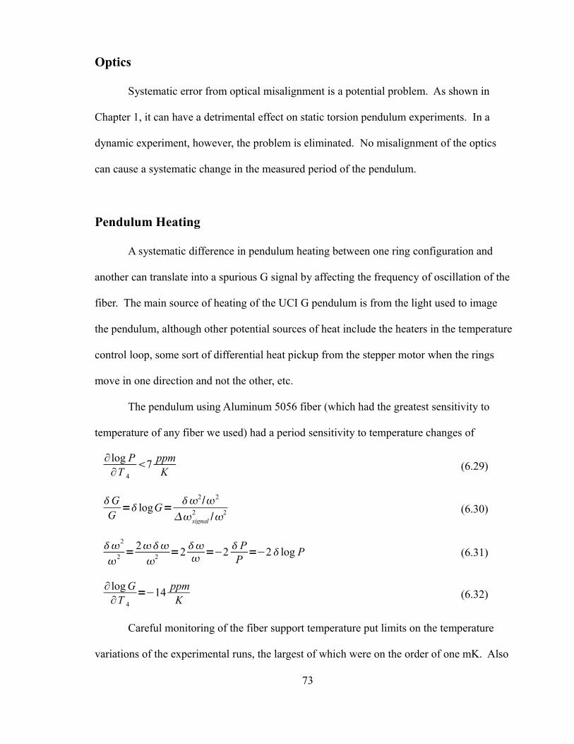
Optics

Systematic error from optical misalignment is a potential problem. As shown in

Chapter 1, it can have a detrimental effect on static torsion pendulum experiments. In a

dynamic experiment, however, the problem is eliminated. No misalignment of the optics

can cause a systematic change in the measured period of the pendulum.

Pendulum Heating

A systematic difference in pendulum heating between one ring configuration and

another can translate into a spurious G signal by affecting the frequency of oscillation of the

fiber. The main source of heating of the UCI G pendulum is from the light used to image

the pendulum, although other potential sources of heat include the heaters in the temperature

control loop, some sort of differential heat pickup from the stepper motor when the rings

move in one direction and not the other, etc.

The pendulum using Aluminum 5056 fiber (which had the greatest sensitivity to

temperature of any fiber we used) had a period sensitivity to temperature changes of

∂ log P∂T 4

7 ppmK (6.29)

GG

= logG=2/2

signal2 /2 (6.30)

2

2 =22 =2 =−2 P

P=−2 log P (6.31)

∂ log G∂T 4

=−14 ppmK (6.32)

Careful monitoring of the fiber support temperature put limits on the temperature

variations of the experimental runs, the largest of which were on the order of one mK. Also

73

reassuringly, the time constant of heat dissipation in the pendulum is on the order of 11

hours, much longer than the ring modulation period of approximately 40 minutes.

Second order couplings

The full set of torques on the pendulum includes the terms

, , A=−k1∑n=2

∞

−k nn−∑

n=1

∞

[n cos nnsin n ]

−k ss [2 A− A2−2]−k ec sin2−0−k visc 2−...

(6.33)

(kss, kec, and kvisc represent the strength of the stick-slip, eddy current, and viscous or “- b v2”

torque on the pendulum).

Torques that affect the frequency to first order include odd-n θn torques, the stick-slip

torque (through its “- 2 A θ” component), and βn torques.

The frequency shift (as well as harmonics, changes in mean angle of orientation or

“offset,” and contribution to 1/Q) from each of these listed torques has been derived

analytically to first order for all of the torques listed in equation 33, and are derived in

Appendices B-E, using the method laid out in Appendix A.

To first order, each of these effects is independent of one another. All frequency

shifts will add linearly, as will contributions to 1/Q, offset, harmonics, etc. Even the G

signal is not affected, to first order, by the presence or absence of any other torques (except,

of course, for the dominant k1 torque). Numerical analysis has shown that this first order

analysis is adequate for a G measurement on the order of 10 ppm, using a method outlined

below.

74

The second order effects of perturbing torques ( for example, k3 or a contribution to

β2 from ambient static gravitational fields) upon one another can be understood qualitatively

in the following way:

The assumption in constructing each of these first-order terms is that each is acting

on a pendulum undergoing perfect sinusoidal motion. But as each term adds its harmonics

to the pendulum behavior, the pendulum's motion deviates from this pure harmonic motion,

and when the second order effects are determined, they must take into account the first-

order harmonics generated by all relevant torques (including the torque whose second-order

effect is being examined). Third-order effects must take into account harmonics generated

by second-order torques, and so on.

To quantitatively evaluate the nonlinear second order effects of the torque terms in

equation 33, we proceed as follows:

First, we define a more concise method of describing the relative strength of the

various torques. We will define the strength of each torque to be ui, where i is some

appropriate index to identify the torque, and ui is the parameter equal to the torque

coefficient divided by k1. So, for example,

uk3=

k3

k1, u4

=4

k 1, etc... (6.34)

Notice that each of these parameters ui is dimensionless, and that a perturbative

treatment is only valid where

u i≪1 (6.35)

The pendulum oscillation frequency will be a function of torsional amplitude A, k1,

and the set of ui parameters. We may Taylor expand that function as follows, where the

coefficients Ci, Dij, Eijk, … are each functions of A.

75

2

02=1∑

iC i ui∑

i , jDi , j u i u j∑

i , j ,kE i , j , k u i u j uk... (6.36)

To first order, we then have

2

02=12

02 =1∑

iC i u iOu2 (6.37)

where, for example,

uk3=

k3

k1;C k3

=34

A2 ;

u4=4

k 1;C 4

=2J 14A

Aetc...

(6.38)

The notation “us” (s for signal) will be reserved for the β2 torque associated with the

source mass rings:

us=2 rings

k1;C s=

2 J 12A A

cos 2rings (6.39)

Note the cos(2 θrings) term in equation 39. During the experiment, the ring positions

are modulated as the ring pair revolves π/2 radians about the pendulum axis and then back

again, causing a sign flip in Cs. It is this sign flip that represents the change in frequency as

the rings are modulated. Rewriting equation 37 to include the s index notation,

2

02=12

02 =1C s us∑

iC i uiOu2 (6.40)

Generalizing to account for second order terms

2

02=12

02 =1C s us∑

iC i u i

D ss us2∑

jD sj us u j∑

i∑

jDi j ui u jO u3

(6.41)

76

This equation does not include a small contribution from the β6 and higher

contribution of the ring source masses to the torque. This contribution is small enough that

it needs to be treated only to first order, and is handled separately in our analysis.

The signal on which our G measurement is based is the difference Δω2signal defined as

the difference between the ω2 values for the two different ring positions. Terms linear in us

change sign in equation 41 when the rings move, contributing the following to Δω2signal:

signal2

02 from us=C s us∑

jD sj us u jOus

3 (6.42)

We see immediately that if the Dsj terms are ignored, the result is an error in G given by:

GG

=2 perturbative effect2ring signal

=D sj Aus u j

C s Aus=

Dsj AC s A

u j (6.43)

Equivalently, a G value found using only the Cs term must be corrected by this amount.

Thus, it is important to evaluate the Dsj coefficients for the perturbing torques which affect

our G measurement.

Equation 42 does not fully account for the signal frequency shift, because there will

be terms in equation 41 which are not proportional to β2 but still change their value when

the rings are moved. Examples are terms proportional to β1 arising from magnetic

couplings, or proportional to β3 arising from small defects in source mass and pendulum

fabrication. Such effects need only be considered to first order, and may be treated

separately.

We now discuss the numerical evaluation procedure used to evaluate the Dsj

coefficients, and their resulting values.

To evaluate the relevant Dsj coefficients, while at the same time testing the

correctness of our analytic evaluation of the Ci and Cs coefficients, we made a set of six

77

numerical integrations of the equation of motion implied by equation 42. Each integration

used a different set of values of ui and us, in the pattern shown by Figure 3.

Figure 6.3: Points Used to Determine Ci and Ds j Cross Terms

The initial angular position of the pendulum in each integration was an arbitrary

value chosen to give the desired amplitude A, while its initial velocity was zero. The

integration tracked the motion of the pendulum through a little more than 1.5 oscillation

cycles, with a minimum accuracy of 10(-14) rad and 10(-14) seconds. The corresponding

frequency ω for each parameter set was determined by finding the time interval between

sequential negative slope zero crossings of the θ(t) function.

The resulting set of six frequencies were then fit to equation 42 to determine the

desired C and D coefficients. This process was repeated for a set of oscillation amplitudes

corresponding to those used in our G measurement. Additionally, for each amplitude, the

derivatives dCj/dA and dDsj/dA were determined by making small variations in the assumed

value of the amplitude A.

78

The resulting C coefficients agreed with those calculated analytically to at least

seven digits, providing an important check of these calculations.

The effect of neglecting higher order terms in the expansion of equation 42 was

probed by increasing the magnitude of the assumed us and ui parameters in the numerical

integration, and found to be negligible.

Resulting values of the C and D coefficients, and their derivatives with respect to A,

are presented in tables 2-5.

79

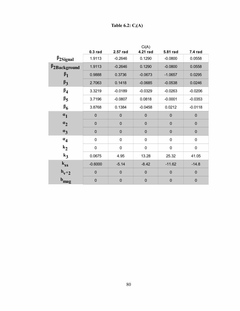
Table 6.2: Ci(A)

80

Ci(A)0.3 rad 2.57 rad 4.21 rad 5.81 rad 7.4 rad1.9113 -0.2646 0.1290 -0.0800 0.0558

1.9113 -0.2646 0.1290 -0.0800 0.0558

0.9888 0.3736 -0.0673 -1.0657 0.0295

2.7063 0.1418 -0.0685 -0.0538 0.0246

3.3219 -0.0189 -0.0329 -0.0263 -0.0206

3.7196 -0.0807 0.0818 -0.0001 -0.0353

3.8768 0.1384 -0.0458 0.0212 -0.0118

0 0 0 0 0

0 0 0 0 0

0 0 0 0 0

0 0 0 0 0

0 0 0 0 0

0.0675 4.95 13.28 25.32 41.05

-0.6000 -5.14 -8.42 -11.62 -14.8

0 0 0 0 0

0 0 0 0 0

β2Signal β2Background

β1β3β4β5β6α1 α2

α3 α4 k2

k3kss

bv^2bmag

Because amplitude varies during the course of a data run, the first derivative of Ci with

respect to A is also relevant:

Table 6.3: dCi/dA (rad-1)

81

dCi(A)/dA0.3 rad 2.57 rad 4.21 rad 5.81 rad 7.4 rad-0.5822 0 0 0 0

-0.5822 0 0 0 0

-0.0744 -0.3544 -0.1464 0.6931 0.0674

-1.8917 0.4362 0.2698 -0.0996 -0.1209

-4.2493 -0.7595 -0.3336 -0.1954 -0.1315

-7.7360 0.8140 0.0304 -0.2547 0.0225

-12.2457 -0.5431 0.3762 -0.2540 0.1834

0 0 0 0 0

0 0 0 0 0

0 0 0 0 0

0 0 0 0 0

0 0 0 0 0

0.45 3.85 6.31 8.71 11.1

-2 -2 -2 -2 -2

0 0 0 0 0

0 0 0 0 0

β2Signal β2Background

β1β3β4β5β6α1 α2

α3 α4 k2

k3kss

bv^2bmag

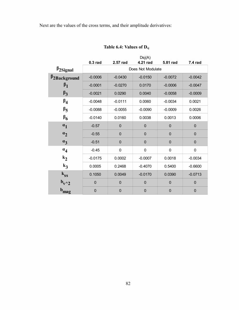
Next are the values of the cross terms, and their amplitude derivatives:

Table 6.4: Values of Dsj

82

Dsj(A)0.3 rad 2.57 rad 4.21 rad 5.81 rad 7.4 rad

Does Not Modulate

-0.0006 -0.0430 -0.0150 -0.0072 -0.0042

-0.0001 -0.0270 0.0170 -0.0006 -0.0047

-0.0021 0.0290 0.0040 -0.0058 -0.0009

-0.0048 -0.0111 0.0060 -0.0034 0.0021

-0.0088 -0.0055 -0.0090 -0.0009 0.0026

-0.0140 0.0160 0.0038 0.0013 0.0006

-0.57 0 0 0 0

-0.55 0 0 0 0

-0.51 0 0 0 0

-0.45 0 0 0 0

-0.0175 0.0002 -0.0007 0.0018 -0.0034

0.0005 0.2468 -0.4070 0.5400 -0.6600

0.1050 0.0049 -0.0170 0.0390 -0.0713

0 0 0 0 0

0 0 0 0 0

β2Signal β2Background

β1β3β4β5β6α1 α2

α3 α4 k2

k3kss

bv^2bmag

Table 6.5: dDsj/dA (rad)

Upper limits have been placed on several values of uj, and the resultant change δG/G

calculated, and presented in table 6.

83

0.3 rad 2.57 rad 4.21 rad 5.81 rad 7.4 radDoes Not Modulate

-0.0084 0.1200 0.0350 0.0160 0.0085

-0.0011 0.0450 -0.0273 0.0040 0.0054

-0.0270 -0.0650 -0.0310 0.0090 0.0090

-0.0600 -0.0320 0.0085 -0.0040 0.0022

-0.1070 0.1100 0.0280 -0.0160 -0.0090

-0.1662 -0.1300 -0.0480 -0.0240 -0.0140

-1.7400 0.2240 0.1070 -0.0260 -0.0270

-1.4900 -0.1880 -0.0520 -0.0220 -0.1200

-1.1020 0.1360 -0.0025 -0.0180 0.0020

-0.6080 -0.0780 0.0275 -0.0130 0.0080

-0.17 2.33 -3.05 3.6 -4.08

0.0065 -0.35 0.45 -0.52 0.57

0 0 0 0 0

-0.0008 0.0100 0.0170 0.0160 -0.1770

0.0056 -0.1690 0.1110 -0.1100 0.0880

dDsj/dA

β2Signal β2Background

β1β3β4β5β6α1 α2

α3 α4 k2

k3kss

bv^2bmag

Table 6.6: Limits on Change in G from Second Order Couplings at Signal Maxima

and 0.3 Rad

(values of over 1 ppm are printed in bold)

84

dG/G predicted (ppm)Value 0.3 rad 2.57 Rad 4.21 Rad 5.81 Rad 7.4 Rad

4.7853E-5 1.0E+6 1.0E+6 1.0E+6 1.0E+6 1.0E+6

3.2600E-2 N/A N/A N/A N/A N/A

1.4356E-5 -4.8E-3 2.33 -1.67 1.3 -1.08

5.5000E-7 -2.0E-5 0.06 0.07 3.9E-3 -0.046

5.5E-7 -0.16 0 0 0 0

1.4E-5 -4.1 0 0 0 0

3.2E-7 -0.030 -2.1E-4 -1.9E-3 -7.3E-3 -0.020

-3.7E-8 -9.5E-6 0.035 0.12 0.25 0.44

-1.4E-7 -3.6E-5 0.13 0.44 0.94 1.65

-6.0E-8 -1.5E-5 0.056 0.19 0.4 0.71

7.0E-7 0.038 -0.013 -0.092 -0.34 -0.89

1.4E-6 0.077 -0.026 -0.185 -0.68 -1.8

1.9E-7 0.01 -0.0035 -0.025 -0.093 -0.24

1.8E-6 0 0 0 0 0

4.0E-5 0 0 0 0 0

Uiβ2Signal/k1

k1 (cgs)β2Background/k1

β1/k1α1/k1α2/k1k2/k1

k3/k1 CuBek3/k1 CuBe H.T.

k3/k1 Al 5056kss/k1 CuBe

kss/k1 CuBe H.T.kss/k1 Al 5056

bv^2/k1bmag/k1

Table 6.7: dLog(G)/dA (rad) from Second Order Couplings

at Signal Maxima and 0.3 Radians

(using the values for uj found in Table 6)

(values of greater than 10ppm per radian are printed in bold)

Other Sources of Error

There are a great many aspects of the UCI G measurement that are not addressed in

this thesis. These include details of data analysis procedures, including (for example) data

cuts based on ring swing amplitudes following transport, cuts on fiber temperature variation,

techniques used to include the protocols for varying ring configurations between run sets to

average out mass density variation effects, and corrections for variation in air density and

ring temperature. And of course, a vast number of details related to mass and dimensional

metrology techniques and their uncertainties have not been discussed.

85

dLog(G)/dA (ppm/rad)Ui Value 0.3 rad 2.57 Rad 4.21 Rad 5.81 Rad 7.4 Rad

4.7853E-5 0 0 0 0 0 k1 (cgs) 3.2600E-2 N/A N/A N/A N/A N/A

1.4356E-5 -0.06 -6.5 3.9 -2.9 2.2

5.5000E-7 -3.2E-4 -0.094 -0.12 -0.028 0.050

5.5E-7 -0.5 -0.47 0.46 0.18 -0.27

1.4E-5 -11.2 10.2 -58 39 -31

3.2E-7 -0.028 -2.9 -7.7 -15 -24

-3.7E-8 -2.4E-4 1.3E-2 -1.7E-2 1.9E-2 -2.1E-2

-1.4E-7 -9.1E-4 4.9E-2 -6.4E-2 7.3E-2 -7.9E-2

-6.0E-8 -3.9E-4 2.1E-2 -2.7E-2 3.1E-2 -3.4E-2

β2Signal/k1

β2Background/k1β1/k1α1/k1α2/k1k2/k1

k3/k1 CuBek3/k1 CuBe H.T.

k3/k1 Al 5056

Chapter 7

Reported Value of G

The experiment used three fibers, and operated at various amplitudes determined by

the maxima of the Bessel function, J1(2A)/A. This allowed us to check the consistency of

the measurement at higher amplitudes where anharmonic torques should produce a greater

effect on the signal. In fact, results were consistent over the range of torsional amplitudes

for each fiber type, but differed significantly among the different fibers used. Expressed as

a ppm difference relative to the current “CODATA” G value (6.67428 x 10-11 m3/kg s2), the

fibers made from CuBe as drawn, heat treated CuBe, and Al5056 yielded G values differing

respectively from CODATA by 26, 8, and 54 ppm, with approximately 13 ppm uncertainty

in each case. (The G values reported at the CPEM 2008 conference were larger by 10ppm

in each case, having omitted a previously calculated 10ppm correction).

Our G measurement was conducted “blind” by hiding the precise value of field

source masses until just before announcing the results. The data taken with the Al5056 fiber

was deemed a priori the more reliable of the three sets, because the Al5056 fiber exhibits the

highest quality factor, the least dependence of quality factor on torsional amplitude, and

yielded the most consistent results at different amplitudes. Hence before removing the

“blind,” we decided to base our announced G value on data taken using the Al5056 fiber,

86

with an uncertainty reflecting the range of G values from the three fiber types. Our final G

value is then larger than “CODATA” by 54 ppm, with an assigned uncertainty of (+25, -42)

ppm. The result adds weight to the 2006 CODATA value relative to a G value reported by a

BIPM group [8], which found G to be greater than the CODATA value by 196 ± 41 ppm.

The value of G reported by the UCI group is 6.67464 (+ .00017, - .00028) x 10-11

m3 /kg s2

87

References

1. H. Cavendish, Esq. F. R. S. and A. S., Experiments to Determine the Density of the Earth. Philosophical Transactions of the Royal Society of London, Vol. 88, (1798), 469-526

2. W. Michaelis, H. Haars, R. Augustin, A new precise determination of Newton's Gravitational Constant. Metrologia 32 (1995/96) 267-276

3. P. J. Mohr, B. N. Taylor, David B. Newell, CODATA Recommended Values of the Fundamental Physical Constants: 2006, National Institute of Standards and Technology, Gaithersburg, Maryland

4. W. Michaelis, H. Haars, J. Melcher, Supplementary investigations to PTB's evaluation of G. Metrologia 41 (2004) L29-L32

5. O. V. Karagioz and V. P. Izmailov, Measurement of the gravitational constant with a torsion balance. Measurement Techniques, Vol. 39, No. 10 (1996) 979-987

6. C. H. Bagley and G. G. Luther, Preliminary Results of a Determination of the Newtonian Constant of Gravitation: A Test of the Kuroda Hypothesis. Phys. Rev. Lett. 78 issue 16 (1997) 3047-3050

7. J. H. Gundlach and S. M. Merkowitz, Measurement of Newton's Constant Using a Torsion Balance with Angular Acceleration Feedback. Phys. Rev. Lett. 85 issue 14 (2000) 2869-2872

8. T. J. Quinn et al., A New Determination of G Using Two Methods. Phys. Rev. Lett. 87 issue 11 (2001) 1101

9. U. Kleinvoss, et al., Measurement of the Newtonian Gravitational Constant G. Precision Electromagnetic Measurements. Conference Digest. Conference on Volume (2002) 148-149

10. T. R. Armstrong and M. P. Fitzgerald, New Measurements of G Using the Measurement Standards Laboratory Torsion Balance. Phys. Rev. Lett. 91, issue 20 (2003) 1101-201104

11. Z. Hu, J. Guo, and J. Luo. Correction of source mass effects in the HUST-99 measurement of G. Phys. Rev. D. 71 issue 12 (2005) 7505-7508

12. St. Schlamminger, et al. Measurement of Newton's gravitational constant. Phys. Rev. D. 74 issue 8 (2006) 2001-2026

13. G. G. Luther and W. R. Towler, Redetermination of the Newtonian Gravitational Constant G. Phys. Rev. Lett. 48 (1982) 121-123

88

14. K. Kuroda. Does the Time-of-Swing Method Give a Correct Value of the Newtonian Gravitational Constant?. Phys. Rev. Lett. 75 (1995) 2796-2798

15. M. K. Bantel and R. D. Newman, Preparation for a Determination of G using a Cryogenic Torsion Pendulum, for the proceedings of the Eighth Marcel Grossman Meeting on General Relativity (1997)

16. R. D. Newman and M. K. Bantel, On determining G using a cryogenic torsion pendulum. Meas. Sci. Technol. 10 (1999) 445-453

17. M. K. Bantel and R. D. Newman. High precision measurement of torsion fiber internal friction at cryogenic temperatures. Journal of Allys and Compounds 310 issues 1-2 (2000) 233-242

18. M. K. Bantel, PhD Thesis, Anelastic behavior of a torsion pendulum with a CuBe fiber at low temperature, and implications for a measurement of the gravitational constant. University of California at Irvine (1998) 19. Z. Hu, J. Luo, Amplitude Dependence of Quality Factor of the Torsion Pendulum, Phys Lett A 268 (2000) 255

20. R. D. Peters, Oscillator Damping with More than One Mechanism of Internal Friction Dissipation, arXiv:physics/0302003 v1 3 Feb 2003

21. A. B. Lebedev, Application of Internal Friction to Analysis of Plastic Behavior of Crystals, Journal de Physique IV, 6 (1996) C8-225-264

89

Appendix A

Perturbation of Harmonic Motion by a Small Nonlinear Force

Term

This appendix describes a method of determining the first-order effect of small

perturbing forces on an oscillator dominated by simple harmonic behavior. Generally, such

forces can change an oscillator's mean position (sometimes called “offset”), change its

frequency, and generate higher harmonics of the fundamental oscillation. In this appendix,

the notation corresponds to a linear harmonic oscillator, such as a mass on a spring. For a

torsion oscillator, force, spring constant, mass, and position are replaced, respectively, with

torque, torsional spring constant, moment of inertia, and angular position.

Consider a simple harmonic force,

F x =−k 1 x (A.1)

yielding the differential equation

F x =m x=−k 1 x (A.2)

with solutions

x t =A sin0t (A.3)

for a frequency defined by 02=

k 1

m and amplitude A. Or, with an appropriate choice of

t,

90

x t =A sin0t (A.4)

Next, consider what happens when a small perturbing force is added to equation 2.

F x =m x=−k 1 xP x , x (A.5)

We will assume that the initial conditions for the solution of this equation yield a peak

oscillation amplitude A such that

∣P x , x ∣k1 A

≪1 for all values of −A≤x≤A (A.6)

The method we will use here to solve this equation is valid only for forces which do not

depend on dx/dt, and thus are not dissipative. Assuming that the solution of equation 5 will

be periodic in t, it can be expressed

x t =A sin t x0a1 cos t ∑n=2

∞

[an cosn t bn sinn t ] (A.7)

We will assume that the phase of the solution is implicitly chosen so that a1 = 0. In addition,

equation 7 must meet the conditions,

∣x0∣≪A∣an∣≪A∣bn∣≪ A

(A.8)

Clearly, x(t) is invariant under the discrete time translations of

t tn 2 , n = 0, ±1,±2,... (A.9)

The second derivative of equation 7 yields

x t =−A2 sin t −∑n=2

∞

n22[an cosn t bn sinn t ] (A.10)

Plugging equations 7 and 10 into equation 5 gives us

91

−m2{A sin t∑n=2

∞

n2 [ancos n t bnsin n t ]}=

k 1{−Asin t − x0−∑n=2

∞

ancos n tbnsin n t }P x (A.11)

Grouping like terms and dividing by m,

k 1 x0−A m2−k 1sin t −

∑n=2

∞

n2 m2−k1[an cos n t bn sin n t ]=P x (A.12)

We recall that the unperturbed frequency is given by

02=

k 1

m(A.13)

In order to proceed any further, P(x,dx/dt) needs to be expressed as a function of time, and

broken down into its Fourier series components:

P t =P x t ≃P Asin t

P t≃A0∑n=1

∞

An cos n t Bn sinn t (A.14)

Note that the approximation in equation 14 expresses x using only the leading (0-order)

term in equation 7. This approximation is permissible for a first-order perturbation of P in x

and dx/dt.

The coefficients in equation 14 are:

A0=2 ∫0

2

P t dt (A.15)

An= ∫0

2

cos n t P t dt (A.16)

Bn= ∫0

2

sin n t P t dt (A.17)

Plugging equation 14 into equation 12 gives

92

k 1 x0−A m2−k 1sin t −

∑n=2

∞

n2 m2−k1[an cosn t bn sinn t ]

=A0A1 cos t B1 sin t ∑n=2

∞

An cos n t Bn sin n t

(A.18)

Again, grouping like terms,

A0−k 1 x0 Am2−k1B1

A sin t A1cos t

∑n=2

∞

{[ann2 m2−k1An ]cos n t [bn n

2 m2−k 1Bn ] sinn t }=0(A.19)

Due to the orthogonality of Fourier series components, this satisfied if and only if each term

leading a sine or cosine is individually equal to 0, and if the constant term is 0, as well.

Note that the A1 Fourier force term is not paired with a Fourier position term. For

conservative forces, the A1 force term is equal to zero, and is not a concern. In fact, a

nonzero A1 term is a valid definition of a nonconservative force. In order to find the change

in energy of a system ΔE from a force P, one needs to integrate the force times distance:

E=∫x1

x2

P x , x ⋅dx=∫t1

t2

P x , x ; t ⋅d xdt

dt (A.20)

For a simple harmonic oscillator,

dxdt=−A cos t (A.21)

and our integral in equation 20 is simplified to

E=∫−P x , x ; t Acos t dt=−A∫P x , x ; t cos t dt (A.22)

This is just equation 16 for n = 1 times a factor of (- A π).

Even for dissipative forces, the A1 term does not produce a change in frequency, an offset, or

any harmonics to first order, but is associated with damping, as will be shown below.

Another treatment that lends itself to a more explicit formulation of damping can be

93

found in Mike Bantel's thesis [18].

In equation 19, the first (constant) term determines the offset (or mean angle):

x0=A0

k1(A.23)

The second term (that of sin(ωt)) determines the frequency (and the frequency change

coming from the perturbation):

2=k 1

m−

B1

A m=0

21− B1

A k1 2

02 =

2−02

02 =−

B1

A k 1

(A.24)

Keep in mind that A is the oscillation amplitude, while Ai and Bi are Fourier

components of the perturbative force as a function of time.

The harmonics of the motion are given by

an=−An

n2 m2−k1

=−An

m1

n22−k 1

m =−

An

m1

n22−02≈−

An

k1

1n2−1 (A.25)

bn=−Bn

n2 m2−k 1

≈−Bn

k 1

1n2−1

(A.26)

where in the previous two equations ω is approximated by ω0 (which is a legitimate

approximation to first order).

Equations 20–23 give the change in frequency, the change in equilibrium point, and

all harmonics, so long as the solutions to equations 15–17 are provided. Later appendices

will simply refer to these equations and plug in appropriate values.

We have now found the frequency shift and harmonics which result from small non-

dissipative torque deviations from an ideal torsion pendulum. As noted earlier, our method

is limited to non-dissipative torques. However, if there are dissipative torque components,

94

we can still find the rate at which the oscillator is damped, and equivalently find the

oscillator's quality factor Q, as follows. Start with the undamped oscillation expressed in

equation 4.

x t =A sin0t (A.4)

we need to find the energy dissipated over the course of a cycle by integrating

E= ∫cycle

P x , x dx

=∫0

2

P t dxdt

dt

=∫0

2

P t Acos t dt

=A[ ∫02

P t cos t dt ] =A A1

(A.27)

To find the effect on 1/Q, we need to divide by the total energy of the system, and divide by

2π to find the fractional energy lost per radian, rather than per cycle:

1 Q =− E

2E

=− A A1

212 k 1 A2 =−

A1

k1 A

(A.28)

We have calculated Δ(1/Q), rather than simply Q, because of convenience: contributions to

1/Q add linearly.

Equation 25 and its exploration here brings up an issue that merits examination: the

basic assumption of this perturbative method is that the motion of the oscillator is periodic,

but obviously this is impossible when dissipative forces are present. Can failing to account

95

for the decaying oscillation lead to errors in the predicted harmonics? We will see that it

should not, by examining the situation where a small perturbative force is added, and the

complete solution can be found analytically: the case of “- b v” damping.

The force is expressed as

P x =−b x=−b v (A.29)

Plugging this into equation 5, we see that

m xb xk 1 x=0 (A.30)

A solution to this equation is

x=A0 e− b

2mtsin t , = k1

m− b2

4m 2 (A.31)

Define the time-dependent amplitude to be

At =A0 e− b

2m t (A.32)

The lowest-order correction to the frequency from the damping term is (from A.28)

2=−b2

4m2 (A.33)

which is second order in b; the first-order treatment described above should not return any

change of frequency. The damping produces no harmonics, and 1/Q is given by

1Q =−E cycle

2 E

=−

12

k 1[A2t=2 −A2t=0]12

k 1 A2t=0

=1−e− b

m

≃ bm

(A.34)

Next, consider what happens when we assume no amplitude decay and use the technique

96

described above. 28 is plugged into equation 14 to find the force harmonics:

P t=−b x=−Abcos t (A.35)

The only nonzero force harmonic is

A1=−A b

12

2

=−A b (A.36)

and all other force harmonics are 0.

As expected, the frequency doesn't change (to first order), nor are any harmonics

generated to first order in b. The only nonzero quantity is 1/Q:

1Q =− A1

k 1 A

=b k1

≃ bm

(A.37)

So to first order in b, the exact treatment and the first-order approximation (assuming

constant amplitude) give exactly the same results: no harmonics, no first-order change in

frequency, and an identical contribution to 1/Q (since the change to 1/Q is a first-order

effect).

97

Appendix B

First Order Perturbative Corrections to Simple Harmonic

Oscillation from Nonlinear Conservative Fiber Torques

This appendix applies the methodology of Appendix A to the particular case where

the torque is purely a function of angle, represented by a Taylor expansion about θ=0. This

will be applied to nonlinear torques on the torsion pendulum arising from properties of the

torsion fiber.

Although the torsion fiber used in the G experiment does have velocity-dependent

torques, a portion of its torques are velocity independent, and may be represented by the

technique laid out in this appendix. This subset of nonlinear fiber torques are termed

“conservative” fiber torques.

Consider a torque dominated by a linear term, perturbed by one small nonlinear term

in θ, of degree m:

I =−k 1−k mm

k m

k1≪1

(B.1)

Because the k1 term dominates, we can assume that the behavior is, to zero order in km,

t =Asin 0 t (B.2)

with ω0 being the frequency with km = 0. Perturbing this with the km term will potentially

98

create an offset, and additional harmonics, and a frequency to be determined later:

t =Asin t a0∑n=2

∞

ancos n t bnsin n t (B.3)

The harmonics in equation 3 form a complete set.

Taking the second time derivative of equation 3,

t =−A2sin t −2∑n=2

∞

n2 [an cos n t bnsin n t ] (B.4)

When solving for the non-fundamental harmonics in equations 3 and 4, we will only find

the solution to first order in km:

km=k m[t ]

m≃k m Amsinm t (B.5)

This approximation is valid for a first-order perturbation. From Appendix A, we can find

the change in offset angle, change in frequency, and the amplitude of all non-fundamental

harmonics if we find the Fourier coefficients of the torque given in equation 5.

To do this, we can make use of the formulas,

sinm t =12

m m!

m2 !m

2 ! 1

2m−1

∑n=2,4,6,. ..

m

−1n2 m!

mn2 !m−n

2 !cos n t , m even

(B.6)

sinm t = 12

m−1

∑n=1,3,5

n

−1n−1

2 m!

mn2 !m−n

2 !sin n t , m odd

(B.7)

so the Fourier coefficients of the torque are (from Appendix A, equations A.15-17)

A0=−k m Am12

m m!

m2 !m

2 !, m even

(B.8)

99

An=−k m Am12

m−1

−1n2 m!

mn2 !m−n

2 !, m and n even;mn0

(B.9)

An=0 , m or n odd (B.10)

Bn=−k m Am12

m−1

−1n−1

2 m!

mn2 !m−n

2 !, m and n odd;mn1

(B.11)

Bn=0 , m or n even (B.12)

Plugging these into Appendix A, equations A.23-26, yields the following:

0=A0

k 1=−

k m

k 1Am 1

2m m!

m2 !m

2 !, m even

(B.13)

2

2 =−B1

A k1=

k m

k1Am−11

2 m−1 m!

m12 !m−1

2 ! (B.14)

an=−An

k1

1n2−1

=k m

k1

Am

n2−1 12

m−1

−1n2 m!

mn2 !m−n

2 ! (B.15)

(m and n even, n > 0)

bn=−Bn

k 1

1n2−1

=k m

k 1

Am

n2−1 12

m−1

−1n−1

2 m!

mn2 !m−n

2 ! (B.16)

(m and n odd, n > 1

an=bn=0 for all other values of m, n (B.17)

Using Appendix A, equation A.28, we can confirm that this is a conservative torque:

no energy is dissipated, shown by the fact that A1 = 0.

From equations 15 and 16, we can see some characteristic effects of a θm torque.

Most obviously, an even-m torque will produce only even cosine harmonics, while an odd-

100

m torque will produce odd sine harmonics. An even m torque will produce an offset angle,

but will not affect the frequency, while an odd m torque will not produce any offset, but will

affect the frequency.

It makes intuitive sense that even-m torques would produce an offset, as they torque

the oscillator in the same direction for both positive and negative θ. It also makes sense that

they should not, to lowest order, affect the frequency, as they are not inherently restorative,

and “push” first towards and then away from equilibrium as the oscillator passes through the

equilibrium point.

Lastly, all harmonics, plus the angle offset or frequency shift, are clearly amplitude

dependent, approaching zero as the amplitude approaches zero. This also makes sense, as

the higher order torques will vanish more quickly than the linear torque as θ → 0, leaving

only a simple harmonic oscillator for any sufficiently small angle.

Table 1 presents the effect of torque perturbations on the form of equation 1, through

m=7, below.

Table B.1: Sample Offset, Change of Frequency, and Harmonics

of km through m = 7

101

m246

m357

a0 a2 a4 a6 -(A2 k2)/(2 k1) -(A2 k2)/(6 k1) -(3 A4 k4)/(8 k1) -(A4 k4)/(6 k1) (A4 k4)/(120 k1) -(5 A6 k6)/(16 k1) -(5 A6 k6)/(32 k1) (A6 k6)/(80 k1) -(A6 k6)/(1120 k1)

Δω2/ω02 b3 b5 b7

(3 A2 k3)/(4 k1) -(A3 k3)/(32 k1) (5 A4 k5)/(8 k1) -(5 A5 k5)/(128 k1) (A5 k5)/(384 k1) (35 A6 k7)/(64 k1) -(21 A7 k7)/(512 k1) (7 A7 k7)/(1536 k1) -(A7 k7)/(3072 k1)

Appendix C

Conservative Field Torques: Offset, Harmonics, Frequency Shift,

Calculation of Coefficients, and Symmetries

This Appendix applies the technique laid out in Appendix A to the special case where

the forces are periodic in x (or torques periodic in θ). It concludes with a discussion of

symmetries of spherical harmonic representations. The technique from Appendix A is used

to consider non-linear torques arising from the pendulum's interaction with static ambient

fields. Such fields might be Newtonian gravitation, electrostatic or magnetostatic forces, or

indeed a new force in nature. In these cases the torque acting on the pendulum is

necessarily a periodic function of the rotation angle of the pendulum. Thus,

I =−k 1 field (C.1)

where

field =−∑m=1

∞

m cos m msin m (C.2)

The minus sign is chosen in order to make this derivation consistent with the notation for

other forces, such as the nonlinear conservative fiber torques in Appendix B.

If the perturbing torque is small, we may assume a dominant sinusoidal behavior for

the pendulum,

0t =Asin 0 t (C.3)

102

We now replace θ in the right-hand side of equation 2 with the approximate θ0(t) given in

equation 3. Then,

field A , , t ≈−∑m=1

∞

m cos[m A sin 0 t]msin [m Asin 0t ] (C.4)

The formalism in Appendix A involves breaking this down into its Fourier components,

t = t , t = t ≃Asin 0 t

t ≃A0∑n=1

∞

An cos n0t Bn sin n0t (C.5)

Applying equations A.15-17 of Appendix A,

A0=2∫0

2

t dt

= 2∫0

2

∑m=1

∞

−{m cos [m Asin t ]msin [mAsin t ]}dt

=−∑m=1

∞

m J 0m A

(C.6)

An0= ∫0

2

t cos n t dt

= ∫0

2

∑m=1

∞

−{mcos [m A sin t ]msin [m Asin t ]}cos n t dt

=−∑m=1

∞

2m J nmA, n even

=0 , n odd

(C.7)

Bn= ∫0

2

t sin n t dt

= ∫0

2

∑m=1

∞

−{mcos [m A sin t ]msin [m Asin t ]}sinn t dt

=−∑m=1

∞

2 m J nmA, n odd

=0 , n even

(C.8)

The above expressions for An and Bn may now be plugged into equations A.25-28 from

103

Appendix A to yield the resultant angular offset, the change in frequency, and the Fourier

coefficients an and bn that describe the harmonics in the motion of the pendulum. The

pendulum's motion is changed from that given in equation 3 to

t =Asin t 0∑n=2

∞

an cos n t bn sin n t (C.9)

The formulas for the offset, frequency, and harmonics are

0=A0

k 1=∑

m=1

∞

−m

k1J 0m A (C.10)

2

2 =−B1

A k1=∑

m=1

∞ m

k 1

2 J 1mAA (C.11)

an=−An

k1

1n2−1

=∑m=1

∞ m

k 1

2 J nmAn2−1

, n even

=0 , n odd(C.12)

bn=−Bn

k1

1n2−1

=∑m=1

∞ m

k1

2 J n mAn2−1

, n odd

=0 , n even(C.13)

As shown in Appendix A, equation A.28, the contribution to 1/Q is proportional to

A1, which is zero. No energy is dissipated by static field interactions.

So far, this treatment applies to torques arising from any sort of static field

interactions. A case of particular importance in this thesis is the gravitational interaction of

a pendulum with ambient mass distributions. We will now show how to find the

coefficients αm and βm first introduced in equation 2 in terms of the mass distributions of a

pendulum and its environment.

Consider a pendulum with mass distribution ρp(x) with x close to the origin. It is in

the presence of a scalar potential Φ(x), generated by a more distant mass source distribution

ρs(x). The potential energy of the system is:

104

U=∫ px xdV p=−G∫sx ' ∫p x 1

∣x−x '∣dV p dV ' s (C.14)

For |x| < |x'|, the 1/|x-x'| portion can be expanded into its spherical harmonic representation,

1∣x−x '∣

=∑l=0

∞

∑m=−l

l

∑l '=0

∞

∑m'=−l '

l ' 42l '1

rl

r ' l '1 Y lm* ,Y l ' m ' ' , ' l ' lm' m (C.15)

Plugging equation 15 into equation 14 yields

U=[∑l=0

∞

∑m=−l

l

∫p x rl Y lm

* ,dV p] ∗[∑l '=0

∞

∑m '=−l '

l '

− 4G2l '1∫

s x ' r ' l '1 Y l ' m' ' , ' dV ' sl ' lm ' m]

(C.16)

First, going through the primed summations (and eliminating the Kronecker δ's),

U=∑l=0

∞

∑m=−l

l

[∫ p x rl Y lm

* ,dV p][−4G2l1∫

sx ' r ' l1 Y lm ' , ' dV ' s] (C.17)

Note that equation 17 is separable into two integrals, with a single summation over l and m.

Defining the pendulum mass multipole moments to be

q lm=∫ px rl Y lm

* ,dV p (C.18)

and the field multipole to be

a lm=−4G2 l1∫

s x r l1 Y lm ,dV p (C.19)

yields

U=∑l=0

∞

∑m=−l

l

q lm alm (C.20)

Next, consider what happens when the test mass undergoes a rotation about the z-axis by an

angle, ψ. We will (for convenience) take the z-axis to be along the axis of rotation of the

pendulum, and roughly parallel to the fiber.

q lmq lm '=∫r , ,−r l Y lm* ,d r (C.21)

105

Using the relation

Y lm* ,=Y lm

* ,−e−i m (C.22)

it becomes clear that

q lm '=∫r , ,−r l Y lm* ,−e−i m d r

=e−i m∫r , ,− rl Y lm* ,−d r

=e−i m qlm

(C.23)

So, when the pendulum is rotated by an angle ψ about the z-axis, the potential energy

becomes

V =∑l=0

∞

∑m=−l

l

qlm a lme−i m (C.24)

with an associated torque of

z=−∂V∂

=∑l=0

∞

∑m=−l

l

i mq lm alm e−i m (C.25)

Next, consider the symmetry of m → - m.

Using the relation from spherical harmonics,

Y lm * ,=−1mY l−m , (C.26)

yields the following:

q lma lm=−4G2l1∫∫s r ' r r l

r ' l1 Y lm ' , ' Y lm* ,d r ' d r

=−4G2l1∫∫s r ' r r l

r ' l1 Y l−m* ' , ' Y l−m ,d r ' d r

=q l−m* al−m

*

(C.27)

Summing the torque listed in equation 24 from both the +m and -m terms and using

equation 26,

106

l ml−m=i mqlm a lme−i mi −m q l−m al−m e i m

=imqlm a lme−i m−i m qlm* a lm

* e i m

=imqlm a lme−i mcomplex conjugate =2ℜi m qlm a lme−i m

(C.28)

So, combining equations 28 and 25, the field torques are:

z=∑l=1

∞

∑m=1

l

2ℜi m qlm alm e−i m (C.29)

As expected, this is a set of sines and cosines of the angle of rotation. Comparing equation

29 with equation 4 yields the following relations:

m=∑l=m

∞

2 mℑq lma lm

m=−∑l=m

∞

2mℜq lm alm(C.30)

Symmetries of the the Spherical Harmonic Representation

There are a number of simple rules that are useful in thinking about spherical

harmonics, and functions of circular symmetry. The first relates to the “m” coefficient in

the qlmalm formulation or, equivalently, the Ylm formulation. The Ylm term can be broken

down into two parts, a polar dependence and an azimuthal dependence.

Y lm ,=Plmcos ei m (C.31)

The eimφ term has m “nodes” where, Re(eimφ) = 0, and the real part flips sign from one

side of the node to the other. Similarly for the imaginary part, though the imaginary nodes

will bisect the angles formed by the real nodes, and vice-versa. Because these nodes are

evenly spaced, it is very easy to conceptualize.

107

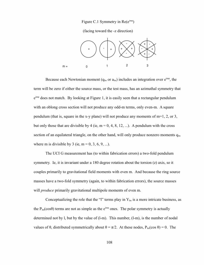
Figure C.1 Symmetry in Re(eimφ)

(facing toward the -z direction)

Because each Newtonian moment (qlm or alm) includes an integration over eimφ, the

term will be zero if either the source mass, or the test mass, has an azimuthal symmetry that

eimφ does not match. By looking at Figure 1, it is easily seen that a rectangular pendulum

with an oblong cross section will not produce any odd-m terms, only even-m. A square

pendulum (that is, square in the x-y plane) will not produce any moments of m=1, 2, or 3,

but only those that are divisible by 4 (ie, m = 0, 4, 8, 12, ...). A pendulum with the cross

section of an equilateral triangle, on the other hand, will only produce nonzero moments qlm

where m is divisible by 3 (ie, m = 0, 3, 6, 9, ...).

The UCI G measurement has (to within fabrication errors) a two-fold pendulum

symmetry. Ie, it is invariant under a 180 degree rotation about the torsion (z) axis, so it

couples primarily to gravitational field moments with even m. And because the ring source

masses have a two-fold symmetry (again, to within fabrication errors), the source masses

will produce primarily gravitational multipole moments of even m.

Conceptualizing the role that the “l” terms play in Ylm is a more intricate business, as

the Plm(cosθ) terms are not as simple as the eimφ ones. The polar symmetry is actually

determined not by l, but by the value of (l-m). This number, (l-m), is the number of nodal

values of θ, distributed symmetrically about θ = π/2. At these nodes, Plm(cos θ) = 0. The

108

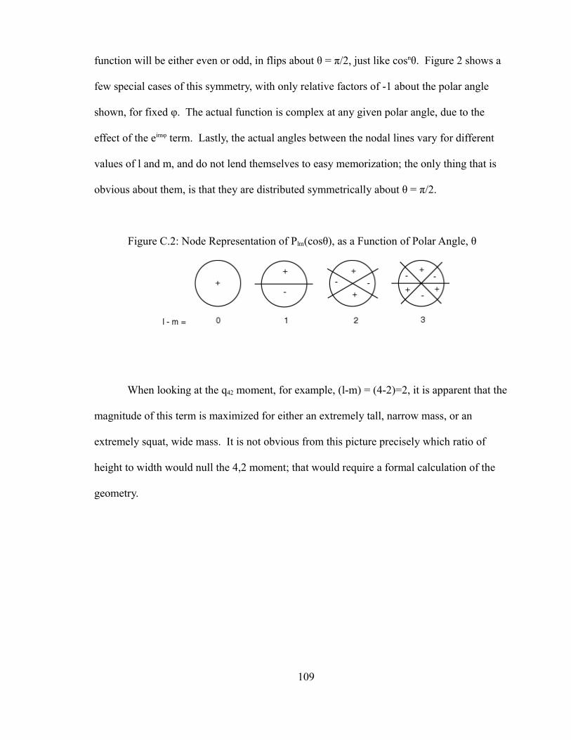
function will be either even or odd, in flips about θ = π/2, just like cosnθ. Figure 2 shows a

few special cases of this symmetry, with only relative factors of -1 about the polar angle

shown, for fixed φ. The actual function is complex at any given polar angle, due to the

effect of the eimφ term. Lastly, the actual angles between the nodal lines vary for different

values of l and m, and do not lend themselves to easy memorization; the only thing that is

obvious about them, is that they are distributed symmetrically about θ = π/2.

Figure C.2: Node Representation of Plm(cosθ), as a Function of Polar Angle, θ

When looking at the q42 moment, for example, (l-m) = (4-2)=2, it is apparent that the

magnitude of this term is maximized for either an extremely tall, narrow mass, or an

extremely squat, wide mass. It is not obvious from this picture precisely which ratio of

height to width would null the 4,2 moment; that would require a formal calculation of the

geometry.

109

Appendix D

The Stick-Slip Model

Studies at the UCI Gravity Lab have found evidence of a “stick-slip” behavior in

torsion pendulums, which has a significant effect on the fiber's harmonics as well as the Q

of its oscillation. In order to explore this effect, we will begin with a linear (rather than

rotational) toy model.

Consider single massive block, coupled to a wall by a spring of constant k1, and also

coupled to the first of an infinite line of massless blocks, each attached to its adjacent blocks

by a spring of constant kss, as shown in Figure 1

Figure D.1

Blocks in a 1-Dimensional Parallel Stick-Slip Model

Note that in this linear model, the stick-slip blocks, and the stick-slip force, are “in

parallel” with the k1 force. The stick-slip system and the “k1” spring are both acting

110

independently on the mass, M. A torsion system that would physically represent this

“parallel” system would be a pair of fibers represented by concentric hollow cylinders, one

of which has a stick-slip behavior, and the other of which has a linear behavior, and neither

of which touch each other (hence the fact that they are in parallel). This distinction is made

now because, later on in this appendix, a “series” stick-slip system will be introduced. We

will now proceed to find the force on the massive block M from the k' spring attached to it.

In this “parallel” stick-slip system, each of the massless blocks, when moved,

experiences a force of friction opposite its movement, of magnitude fss. This frictional force

is independent of velocity, and will serve to keep the block fixed in place if the absolute

value of the sum of all other forces on the block is less than fss.

Define the distance between stick-slip block i and the wall as xi, with x being the

position of the massive block. The force on the massless stick-slip block i will then be

F ix i−1 , x i , x i1=−k ' [xi−xi−1−x i1− x i]=k ' x i1x i−1−2 xi (D.1)

and the force on the massive block M at position x due to the stick-slip perturbation will be

F ss x , x1=−k ' x−x1 (D.2)

Let us also define the a fundamental unit of length for this system,

x≡f ss

k '(D.3)

Given a system with x = 0 and all xi = 0, this is simply the maximum amount you could

move any one block (including the massive block) without moving any of the others.

Note that, in order for this system to behave like a simple harmonic oscillator, to 0th

order in kss, there would have to be a restriction, namely,

F ssx=A≪k 1 A ; (D.4)

In the simplest case, consider what would happen if the largest block were to

111

oscillate at an amplitude A = Δx, with x1(t) = 0 (ie, the first stick-slip block never moves).

In that case, the nearest block would never move, no energy would be dissipated by the

system, and the stick-slip force equation would be trivial:

F ssx =−k ' x (D.5)

Next, consider what would happen if the amplitude of the oscillation of M were large

enough to move the first stick-slip block a maximum distance of Δx from its equilibrium

point, or just enough so that block 2 does not move at all.

The following analyses will only apply to circumstances where block M moves

monotonically from some negative extremum to some maximum, stops, and then moves

monotonically back to its negative extremum, etc. This is because the stick-slip force on

block M, as a function of position, will be a hysteresis loop, and any motion that does not

behave in this monotonic fashion will explore the interior of this loop, rather than the

perimeter. Such behavior is beyond the scope of this derivation.

At t=0, both block M and block 1 are at their negative extrema, with block M's

coordinate,

x 0=−A=−2 x (D.6)

and about to begin moving in a positive direction. Block 2 will be at

x2t =0 for all t (D.7)

since it does not move. Block 1 will be at the maximum negative displacement possible

without moving block 2:

x1t=0=− x x2=− x (D.8)

and by equations 1, 7, and 8,

112

F1t=0k '

=−f ss

k '=− x= x2x 0−2 x10=x 02 x ;

x 0=−3 x(D.9)

As block M is moved to the right, the force will at first be described by the equation,

F ssx ; v0=k ' x1− x=k ' − x− x=−k ' x x, −3 xx− x (D.10)

Once x reaches –Δx, block 1 will begin to slip from its position. Once block 1 begins to

slip, the stick-slip force upon block M will depend on the value of x1. From this point

onwards, the force on block 1 will be + kss Δx, and by equation 1,

F 1=k ' x=k ' x2 x−2 x1=k '∗x−2 x1 (D.11)

or

x1x ; v0= x− x2,

− xx3 x (D.12)

Thus the force on block M is (by equations 2 and 12)

F ssx ; v0=−k ' x−x1=−k ' x− x− x2 =−k ' x x

2 , − x x3 x (D.13)

So, from equation 13, we have the stick-slip force on the massive block for a single slipping

block as a function of position for the positive velocity portion of the oscillation.

For the negative velocity part of the oscillation, by a similar technique,

F ssx ; v0=−k x− x , xx3 x (D.14)

and

F ssx ; v0=−k ' x− x2 , −3 x x x (D.15)

The amount of energy dissipated by this system is simply the integral of the force over these

four regions:

113

E= ∫−3 x

− x

k ' x xdx ∫− x

3 x

k ' x x2 dx

∫3 x

x

−k ' x− x ∫ x

−3 x

−k ' x− x2 dx

=k ' x2 [2−42−4 ]E=−4k ' x2

(D.16)

This result makes intuitive sense, as the force on block 1 as it slides is – k' Δx = -fss, and it

slides a total distance of 4 Δx, equal to twice its peak-to-peak amplitude of oscillation. This

is shown graphically in Figure 2.

Figure D.2

Stick-Slip Force for a One Slipping Block System

Fss/(k'Δx)

x/Δx

Note that a hysteresis loop has already emerged from this simple model. The area of this

loop is the energy dissipated, as calculated in equation 16.

Next, consider the case where N of the stick-slip blocks move as the massive block

M oscillates between its extrema.

114

The Nth block will have an amplitude of Δx, like block 1 in the above example. The

(N-1)th block has an amplitude of 3 Δx like the massive block in the above example, the (N-

2) block must (by equation 1) have an amplitude of 6 Δx, and the (N-3) block 10 Δx, etc.

The (N-n)th block will slide a peak-to-peak amount of twice its amplitude,

max x N−n−min xN−n=n1n2 x (D.17)

By equation 17, block M (at position 0 = N-N) will oscillate with an amplitude of

A=N 1 N22

x (D.18)

Consider what will happen when the massive block is at the negative extremum, as it begins

to move with positive velocity. It will at first experience a force,

F ss−A=k ' x1min− x0min=k ' x{−N N12

−[−N1 N22 ]}

=k ' x[− N 2N2

N 23N22 ]=N1k ' x

Fmax≡N1k ' x

(D.19)

Equation 19 should be intuitively obvious: N+1 springs are under compression, with the

tension stepping up by exactly k' Δx on each successive spring, and the final spring exerts its

force on the massive block, expressed as Fss.

As the massive block begins to move, this force will diminish linearly for a distance

2 Δx. By equation 2,

F ss x ; v0=−k ' [N1 x−xA], −A x−A2 x (D.20)

at which point the first massless block will begin to slip, generating a new, slightly more

shallow slope, until the second block begins to slip, which will generate an even shallower

slope. The net force on any slipping block is + k' Δx. So, for block 1, using equation 1,

F 1x1, x2, x =k ' x=k ' x2t x t −2 x1 t (D.21)

115

which yields

x1x2, x =12x2x− x (D.22)

Plugging equation 2 into equation 22 yields

F ssx ; v0=−k2 x t −x2 0 x ,−A2 x x0−A6 x (D.23)

In equation 23, we have eliminated the explicit dependence upon the position of the moving

block, x1, and only look at the position of x2, which is fixed over this region. A repeated

application of this method produces a telescoping series revealing Fss, such that when block

m breaks free,

F ssx ,m ;v0=[ x m1t=0m1

−m x2 − x0

m1 ]k '

,−Amm1 x x0−Am1m2 x(D.24)

where, by equation 18,

A=N 1 N22

x (D.25)

and, using equation 17,

xm t=0=xm t tm=−N−m1 N−m22

x (D.26)

until the block begins to move at time tm.

When looking at the change in Fss over this range, we can look at the change in force

between the beginning and end of the range. For instance,

F ss m=0=2 x k '−0 x k '=2 x k ' (D.27)

While, for m = 1,

F ss m=1=126 x−2 xk '=2 x k ' (D.28)

116

In general, using the maximum and minimum values of x in equation 23,

F ss m= 1m1

−Am1m2 xA−mm1 x k '

= x k 'm1

m23m2−m2−m=2 x k '(D.29)

which leads to

F ssm ,v0=F max−∑i=0

m

2 x k '=[N1−2m ] x k ' (D.30)

Thus, the stick-slip force is linear in m, the number of blocks that have broken free.

Equivalently,

F ssm ,v0=F max−∑i=0

m

2 x k '=[N1−2m ] x k '

m= N12

−F ss

2 k ' x

m=Fmax−F ss

2 k ' x

(D.31)

Finding the average value of x(m),

x m , v0 =12[−Am1m2 x−Am m1 x ]

=−Am22m1 x

=[−12N1N2 xm12 x ]

(D.32)

Combining equations 31 and 32 to eliminate m and find x as a function of Fss,

x F ss , v0=−12N12 x−N1

2 xm22m1 x

=−F max

2

2 k ' 2 x

F max2

4k ' 2 x

F ss2

4 k ' 2 x−

F ss F max

2k ' 2 x

F max

k '−

F ss

k ' x

=−F max

2

4k ' 2 x

F ss2

4 k ' 2 x−

F ss F max

2k ' 2 x

F max

k '−

F ss

k ' x

x F ss , v0≈ 14 k ' 2 x

[F max2 −F ss

2 −2 F ss F max]

(D.33)

When the force is a maximum, pushing to the right, the position is at the negative

117

extremum, and vice versa.

More generally,

x F ss ≈−1

4k ' 2 x[2 F ss F maxv F ss

2 −F max2 ] (D.34)

This is confirmed by an independent derivation [18, p. 98 ]. It can be re-expressed as

F ssx =−v F max−2 F max2 −v 4 k ' 2 x x (D.35)

Setting x = A to find Fmax gives us

F max=k ' 2 A x (D.36)

yielding a better version of equation 35:

F ssx =−v k ' 2A x−2 k ' x A−v x (D.37)

Let us now define, for the parallel stick-slip case,

k ss=k ' 2 x (D.38)

and rewrite equation 37 as

F ssx , v=−v k ssA−2 k ss A−v x (D.39)

Here is a plot of equation 39:

118

Figure D.3

Fss(x) for a Large Number of

Stick-Slip Blocks

1.0 0.5 0.5 1.0x A

1.0

0.5

0.5

1.0

Fss

Fmax

This linear system can easily be generalized to a torsion system, with a series of zero-inertia

cylindrical shells playing the role of the massless blocks. Let the stick-slip torque perturb a

system's simple harmonic motion:

I =−k 1−v k ss A−2A−v (D.40)

Or, expressed as a function of time,

ss t =−v k ss A−2 A−v A sin t =−v k ss A 1−21−v sin t (D.41)

The formalism in Appendix 1 involves breaking this torque down into its Fourier

components,

ss t =A0∑n

An cos n t Bnsin n t (D.42)

The formulas to calculate these torque coefficients are in Appendix A, equations A.15-17:

A0=2 ∫0

2

ss t dt= 2 ∫0

2

−v k ssA−2A−v Asin t cos n t dt=0 (D.43)

119

An= ∫0

2

sst cos n t dt

= ∫0

2

−v k ssA−2 A−v A sin t cos n t dt

=0 , n even

=4−1

n−12

n4n2−1k ssA, n odd

(D.44)

Bn=∫0

2

ss t sin n tdt

= ∫0

2

−v k ss A−2 A−v sin n t

=8−1

n12

4n2−1k ssA , n odd

=0 , n even

(D.45)

Plugging these into Appendix A, equations A.23-26, yields:

0=A0

k 1=0 (D.46)

2

2 =−B1

A k 1= 8

3k ss

A(D.47)

an≥2=−An

k 1

1n2−1

= 4

−1n1

2

n 4n2−1n2−1k ss

k1 A , n odd

=0 , n even

(D.48)

bn≥2=−Bn

k1

1n2−1

= 8

−1n−1

2

4n2−1n2−1k ss

k 1A, n odd

=0 , n even

(D.49)

The effect on Q can be derived in a straightforward manner using Appendix 1,

equation A1.28

120

1Q ss

=−A1

k 1 A

= 43

k ss

k1

1A

(D.50)

However, experiments at the UCI gravity lab [17] have shown that to a good approximation,

1Q ∝A (D.51)

Therefore, the model presented above cannot be a significant contribution to 1/Q. However,

a variation of this model is potentially viable.

Consider what would happen if Figure 1 were altered so that the long series of stick-

slip blocks were located between the massive block and the immobile wall.

Figure D.4

Stick-Slip Blocks in a Series Configuration

Note that the system is now “in series.” The mass is coupled through the linear spring to the

stick slip system, and from there to the wall. Neither the stick-slip system nor the k1 spring

can be severed without decoupling the massive block from the wall entirely. From this

point onward, the derivation of the stick-slip behavior will follow the path presented in

Mike Bantel's thesis, chapter 7, p. 98. For a torsion effect, this would occur if the fiber itself

121

were anchored by a “stick-slip” region to its mount.

Consider equation 34, reproduced here:

x F ss ≈−1

4k ' 2 x[2 F ss F max−v F max

2 −F ss2 ] (D.34)

This formula does not involve any approximations, beyond the assumption of a large

number of stick-slip blocks. It is equally applicable to both the series and parallel situations.

Then, consider the effect of the following approximation, which are necessary in the case of

a “series” stick-slip torsional force:

ss =−k 1max=−k1 A (D.52)

The stick-slip torque no longer acts directly on the pendulum. Instead, the stick-slip region

acts as an additional spring, extending and contracting to alleviate the tension or

compression on the k1 spring. The relevant differential equation becomes:

I =−k 1−ss (D.53)

where θss is defined by equation 34:

ss ss=−1

4 k ' 2 x[2ssmax−max

2 −ss2 ] (D.54)

Plugging equation 55 into equation 57 yields:

ss =−1

4 k ' 2 x[2 k1

2 A− k12A2−2] (D.55)

which, when plugged into equation 53, yields the effective stick-slip torque:

ss=I k1=k1

3

4 k ' 2 x[2 A− A2−2] (D.56)

This equation has both a linear amplitude-dependent correction of the k1 term (a

conservative torque that affects frequency but no harmonics), and a stick-slip term with a

122

force-hysteresis loop shown in Figure 5. Let us renormalize the k', Δx, and k1 terms, and

create a single stick-slip term to represent them:

ss =2 A k ss− k ss A2−2 (D.57)

ss t =2 A2 k sssin t −A2 k ss [1−sin2 t ] =A2 k ss [2sin t − cos2 t ] (D.58)

Figure D.5

Torque as a Function of Amplitude

for a Small Series Stick-Slip Effect

In order to find the harmonics, we again turn to Appendix 1, equations A1.15-17, and find

the time-series harmonics of the stick-slip force:

A0=2 ∫0

2

t dt=0 (D.59)

123

-1 -0.5 0.5 1A

-1

-0.5

0.5

1

ss max

An= ∫0

2

t cos n t dt

= ∫0

2

A2 k ss [2sin t − cos2 t ]cos n t dt

=8−1

n12

nn2−4A2 k ss , n odd

=0 , n even

(D.60)

Bn= ∫0

2

t sinn t dt

= ∫0

2

A2 k ss [2sin t − cos2 t ]sin n t dt

=2A 2 k ss , n =1 =0 , n≥2

(D.61)

The Fourier torque coefficients given in equations 59-61 can be used to determine the shift

in frequency and Fourier harmonics of the pendulum using Appendix 1, equations A.23-26:

0=A0

k 1=0 (D.62)

2

2 =−B1

A k 1=−2 A

k ss

k1(D.63)

an≥2=−An

k1

1n2−1

=8−1

n−12

nn2−4n2−1A2 k ss

k 1, n odd

=0 , n even

(D.64)

bn=0 (D.65)

As shown in Appendix 1, equation A.28, the contribution to 1/Q is proportional to A1:

1Q ss

=−A1

k1 A

= 83

k ss

k 1A

(D.66)

124

This gives the a contribution consistent with the findings of Newman and Bantel

[17].

Some harmonic coefficients of this behavior are given, below.

Table D.1

an For Series Stick-Slip Effect

Note that equation 57 can be expressed as two dissipative terms, one proportional to A2, and

the other proportional to θ2. Both of these contribute to the linear dependence of 1/Q on A.

In practice, almost any force with a contribution to 1/Q that is linear in amplitude

will be an acceptable torque candidate. Multiplying either the A2 or the θ2 term in the stick-

slip torque by any dimensionless function f(A/θ) will also result in an acceptable torque

profile. In the absence of a measurement of the shape of the stress-strain loop (figures 5, 3,

and 2), it is difficult to determine the profile of the torque that generates it [21]. This

derivation is an attempt to impose some physical model on the behavior of the pendulum,

but in fact the torque profile that produces our measured dependence of 1/Q on amplitude is

unknown.

125

n

3 1/(15π)5 -1(315/π)7 1/(1890π)

an*(k1 /kss A2)

Appendix E

An Examination of the Effect of a Magnetic Field on Pendulum

Damping

Consider a region of uniform, static magnetic field,

B=B0cos0 xsin0 y (E.1)

In this field hangs a thin, flat, nonconductive pendulum painted with a thin conductive ring of

resistivity ρ centered about the center of mass of the pendulum. The ring's radius is “r,” its

thickness is “ε,” and its width is “dr.” The ring encloses an area S = π r2, and a circuit around

the ring has a total resistance of

R= 2 r dr (E.2)

The orientation of the pendulum is

n=cos xsin y (E.3)

The angle ψ0 in equation 1 describes the angle made by the magnetic field and the normal

vector to the pendulum when it (the pendulum) is at rest. The z-axis is parallel to the axis of

rotation.

The pendulum's behavior in the absence of a magnetic field is described by a simple

harmonic oscillation of frequency ω0 and amplitude A.

0t =Asin 0 t (E.4)

126

The magnetic flux passing through the pendulum as a function of angle is

=S B⋅n=B0 S cos0 cossin0sin (E.5)

As the pendulum rotates, it induces a magnetic current,

I=− 1R

d d t

=− 1R

S B0 −cos0 sinsin0 cos d d t (E.6)

This current generates a magnetic moment of

, =I S n=− 1R

S 2 B0[−cos0sin sin0 cos] d d t

n (E.7)

The torque is straightforward to calculate:

, = , ×B

=−1R

S 2 B02[−cos0sin sin0 cos]d

d tcos xsin y×cos0 xsin0 y

=−1R

S 2 B02−cos0 sinsin0 coscossin0−sincos0

d d t

z

=−1R

S 2 B02 d d t

[sin2−0]z

(E.8)

For convenience, we will use

bmag≡1R

S 2 B02 (E.9)

to describe the strength of the torque, in analogy with “- b v” style damping.

Plugging in equation 1 in order to find the torque as a function of time,

t=−bmag sin2−0=−bmag A cos t sin2[A sin t −0] z (E.10)

Using appendix A, equations A.15-17 to find the Fourier components of the torque, to express

it as

zt =A0∑n=0

∞

An cos n t Bnsin n t (E.11)

with coefficients

127

A0=2 ∫0

2

zt dt=0 (E.11)

A1= ∫0

2

zt cos t dt

= ∫0

2

−bmag A cos t sin 2[A sin t −0]cos t dt

=−bmag2 A−cos [20] J 12A

(E.12)

An1= ∫0

2

z t cos n t dt

= ∫0

2

−bmag Acos t sin2[Asin t −0]cos n t dt

=bmag2

cos 20n J n2A , n odd

=0 , n even

(E.13)

Bn= ∫0

2

z tsin n t dt

= ∫0

2

−bmag Acos t sin 2[Asin t −0]sinn t dt

=bmag2

sin 20n J n 2A, n even

=0 , n odd

(E.14)

Now that we have the time-series torque effects, we can apply these to determine the

measurable pendulum behavior: offset, change in frequency, harmonic oscillations, and

energy dissipation using Appendix A, equations A.23-A.26.

2

02 =−

B1

A k1=0 (E.15)

0=A0

k 1=0 (E.16)

128

an=−An

k1

1n2−1

=−bmag

k 1

2

cos20n

n2−1J n2A , n odd

=0 , n even

(E.17)

bn=−Bn

k 1

1n2−1

=−bmag

k 1

2

sin 20n

n2−1J n2A, n even

=0 , n odd

(E.18)

1 Q =− A1

k 1 A

=bmag

k 1

2 1−cos [20]

J 12A A

(E.19)

So the eddy currents do not offer simple “-bv” type damping of the pendulum, but produce

harmonics and amplitude-dependent damping.

Applications to the UCI G pendulum

The relationship between the model presented here and that of the square G pendulum

is not obvious. The path of electrons for a square pendulum of finite thickness undergoing

harmonic oscillation is not simple to calculate, and will not be attempted, here. However, we

can deal with the special case of a flat disc-shaped pendulum of area S = π r2 where the

electric current is constrained to flow in concentric, circular paths about the center of mass of

the flat pendulum. While this may not give the exact eddy current damping value for the

pendulum, it should give an answer that is accurate to within a close order of magnitude.

First, combining equations 8 and 2,

129

, =−∫0

r

2 r ' [r ' 2]2 B0

2 d d t

[sin2−0]dr '

=−2

B02 d

d t[sin2−0]∫

0

r

r ' 3 dr '

=−8

r 4 B02 d

d t[sin 2−0]

=− 18

S 2 B0

2 d d t

[sin2−0]

(E.20)

This gives an “interaction strength” of

bmag=1

8

S 2 B02 (E.21)

For the UCI G pendulum, S = 1.6 * 10-3 m2. For 4K, ρAl = 1.1 * 10-12 Ω m [23], and ρAu = 2.2

* 10-10 Ω m [24]. Although the temperature of the UCI G pendulum was between 2K and 4K,

this should not affect the resistivities, as they were quite insensitive to changes in temperature

in this range. The aluminum layer has a thickness of 100 nm on each side, while the gold is

approximately 200 nm thick on each side. Although the gold is thicker, its two orders of

magnitude greater resistivity at this temperature make its contribution to the eddy current

damping small compared with that of the aluminum, and so it will be ignored. While

differential changes in the vicinity of the pendulum are quite small (see chapter 4), the full

field strength is not well known. Assuming (as an upper limit) that the magnetic field in the

vicinity of the pendulum is roughly equal to the ambient magnetic field of the earth (5 * 10-5

Tesla), we find that

bmag=1

82.0∗10−7 m

1.1∗10−12m∗1.6∗10−3 m225.0∗10−5 T 2

=4.6∗10−11T 2/=4.6∗10−11 kg m2/ s(E.22)

For a value of k1 = 3.3 * 10-9 kg m2/s2 and ω = 2 π/(135 s) = .047 / s, this gives us a value of 1/

Q of (from equation 19)

130

1 Q =bmag2 k1

=4.6∗10−11 kg m2 /s .047 /s

2∗3.3∗10−9 kg m2/s2 1−cos [20]J 12A A

=3.3∗10−41−cos [20]J 12A A

(E.23)

At extremely low amplitudes, 1/Q = 3.3 * 10-4 ± 100% (depending on magnetic field

orientation), corresponding to a Q of at least 1500 and possibly much greater. At 7.4 radians,

1/Q is very close to 3.3 * 10-4 ± 3%, which could contribute to a Q of no more 3000

(depending on magnetic field orientation). This is smaller than the observed Q of 80,000+ by

a factor of about 27.

Because an 0.5 gauss field has such a deleterious effect on Q, we can work backward

from the observed Q to see what upper limit this places on B0. By equation 21, bmag is

proportional to B02, so in order to decrease the contribution to 1/Q by a factor of 27, we need

to attenuate the assumed magnetic field by a factor of at least 5. Therefore the upper limit

placed on the magnetic field by eddy current damping is approximately 1*10-5 T.

Studies of the UCI G experiment (see chapter 4) find that changes in external magnetic

fields are attenuated by a factor of 2,000. While this does not tell us what internal magnetic

fields may be present, it suggests that the field may be a factor of 2,000 less than the 0.5 gauss

assumed for equation 22. If that were the case, then rather than getting a contribution to 1/Q

of 3.3*10-4, it would be a contribution of 3.3*10-4/(2*103)2 = 8.3*10-11. This would only be a

significant contribution to damping for a Q on the order of 1010, six orders of magnitude larger

than the observed value of Q.

131