UNIVERSITY OF CALIFORNIA Los Angeles Dynamic Modeling

UNIVERSITY OF CALIFORNIA

Los Angeles

Dynamic Modeling

of the High Purity Oxygen

Activated Sludge Process

A thesis submitted in partial satisfaction of the

requirements for the degree Master of Science

in Civil Engineering

by

David Bryan Whipple

1989

The Thesis of David Bryan Whipple lS Approved.

J.B. Neethling

M.K. Stenstrom, Committee Chair

University of California, Los Angeles

1989

ii

TABLE OF CONTENTS

Introduction

Literature Review

Model Development

Model Calibration

Plant Studies

Conclusions

References

Appendix

Model Parameters

Computer Program

iii

PAGE NUMBER

1

3

8

18

27

42

45

49

51

LIST OF FIGURES

Figure 1

Figure 2

Figure 3

Figure 4

Figure 5

Figure 6

Figure 7

Figure 8

Figure 9

Figure 10

Mass transfer and the basic substrate

reaction for stage (i)

Final stage dissolved oxygen

concentration, constant liquid and gas

flow rates


concentration, controlled gas flow rate.

Influent gas feed rate, constant liquid

feed rate.

Final stage dissolved oxygen , fixed gas

feed rate, sinusoidal liquid feed rate.

Final stage dissolved oxygen , controlled

gas feed rate, sinusoidal liquid feed

rate.



rate.

Influent gas feed rate with sinusoidal

liquid feed rate.

Final stage dissolved oxygen below the

established minimum.

Final stage dissolved oxygen for

variable and fixed gas flow.

iv

LIST OF TABLES

Table 1

Table 2

Table 3

Table 4

Table 5

Table 6

Warranty conditions.

Operating conditions adjusted to warranty

conditions for comparison.

Physical dimensions of the aeration

basins.

Oxygen transfer coefficient for the.

surface aerators.

Error in model prediction.

Steady state influent parameters for

capacity simulation.

v

ACKNOWLEDGEMENT

I would like to thank Dr. Michael Stenstrom for his

assistance in the development and completion of this

work. I would especially like to acknowledge his

understanding of the unique situation presented to the

working student.

I would like to thank Mr.Bill Kimble and Mr.Fred Yunt of

the County Sanitation Districts of Los Angeles County

for providing the data, and operational information.

Without which, this project would not have been

possible.

I would also like to express my appreciation to my

family and friends for their support throughout my

academic adventures.

vi

l

ABSTRACT OF THE THESIS

Dynamic Modeling

of the High Purity Oxygen

Activated Sludge Process

by

David Bryan Whipple

Master of Science in Civil Engineering

University of California, Los Angeles, 1989

Professor Michael K. Stenstrom, Chair

This thesis uses a dynamic model to quantify the

capacity of the high purity oxygen activated sludge

process. The Joint Water Pollution Control Plant in

Carson California was used as an example plant. Data

collected in May, 1984 during a full scale test of this

facility were used to calibrate the dynamic mathematical

model. Following calibration, the model was used to

simulate process performance. Specifically, the model

was used to determine the treatment capacity of the

activated sludge reactors. The results of the computer

vii

simulation indicate that the original design capacity

can be exceeded by sixty percent (80 million gallons per

day maximum) including a twenty percent sinusoidal

diurnal flow fluctuation. However, those conditions

were achieved during a simulation that included

automatic oxygen flow control based on the fourth stage

dissolved oxygen concentration. Under those conditions,

the fourth stage dissolved oxygen concentration never

declined below 3.0 mg/1. It was concluded that,

although the Carson plant is currently under loaded, any

increase in the influent wastewater flow rate must

consider the resulting decreasing sludge age, and the

possibility of increased instability from industrial

waste.

viii

I INTRODUCTION

During the past several years, the Environmental

Protection Agency working under the Clean Water Act has

begun to enforce the requirement that all sewage

treatment conform to secondary effluent standards. The

current favored technology for municipalities is the

activated sludge process. The activated sludge process

presents two operational options: aeration using air as

the oxygen transfer fluid, or a contained vessel using

high purity oxygen. The high purity process option

presents two distinct advantages. The plant requires a

significantly smaller geographic area than an air plant

treating the same waste flow. Secondly, the high purity

system uses covered reactors. The covered reactors may

be advantageous in the control of volatile emissions.

In 1984 the County Sanitation Districts of Los Angeles

County began operation of a high purity oxygen activated

sludge plant in Carson California. The original plant

provided advanced primary treatment for 360 million

gallons per day (MGD) of combined industrial and

domestic sewage. The secondary system comprised four

treatment trains. Each train was designed to treat 50

MGD . A treatment train consists of four 1.315 million

gallon complete mix reactors in series. Oxygen is

transferred by three surface aerators per reactor. To

1

provide the required oxygen, the County built two 150

ton per ·day cryogenic oxygen plants. During May of 1984

the County tested the oxygen transfer capability of the

secondary treatment system to verify the warranty

requirements of the purchase contract. The test results

indicated the plant had transferred more oxygen than

required by the warranty.

During verification testing, the County collected a

significant amount of operational performance data.

This thesis uses the historical data provided by the

County and applies a dynamic mathematical model to

predict operational performance and plant capacity. The

model was written in Fortran and CSMP III.1 CSMP III is

a mathematical computer program designed to solve

differential equations.

The significance of such a predictive tool is its future

application by municipalities and industry to determine

if their current a~tivated sludge plants have additional

capacity. Additional capacity will be required in the

future as the Environmental Protection Agency enforces

the Clean Water Act. Additionally, predictive tools of

this nature allow design engineers to determine future

capitol investment as a function of projected required

capacity.

2

II LITERATURE REVIEW

Early work in mathematical modeling of the activated

sludge process involved the application of mass and

microbial balances to steady state processes. The model

of Mueller, Mulligan, and di Toro2 was based on those

conditions. The model described the transfer of oxygen,

nitrogen, and carbon dioxide between the gas and liquid

phases, but did not account for nitrificat.ion.

Therefore the total ammonia nitrogen concentration

remained constant. Additionally, given the absence of

nitrification and the assumption that all biologically

produced C02 remains as C02, eliminated any significant

alkalinity source or sink. The model was calibrated to

an operating high purity oxygen process. The model was

then applied to predict plant performance utilizing

several sets of constant (time- invariant) feed

conditions.

Gaudy, Srinivasaraghavan, and Saleh developed a steady

state algorithm to account for the variabilities in the

concentration of the biological solids through control

of the return sludge concentration.3 The Monod growth

equation was used to model substrate removal. Gaudy

assigned effluent substrate concentration as the basis

for plant efficiency evaluation. He concluded that

system engineering variables had a greater impact on

3

process dynamics than changes in the biological

constants.

The development of a true mul ticomponent mass transfer

model of the gas-liquid interface was presented by

McWhirter and Vahldieck.4 Initial development of the

model included coupled equations. However, following the

assignment of ideal conditions to the gas phase, and

considering the dilute nature of the liquid phase

concentrations the equations became non-interactive.

Equations for tne C02 gas/liquid equilibrium were based

on the assumption that all non-ionized C02 was dissolved

rather than in the form of carbonic acid. The equation

for alkalinity was developed as a function of system pH

and the mole fraction C02 in the gas phase. A complete

set of equations were presented for gas/liquid component

mass transfer. The gas purity predictions were then

compared to an operating UNOX plant. The data indicate

a very good fit.

Stenstrom and Andrews5 presented a development of

mathematical process control strategies for dynamic

activated sludge operations based on SCOUR, the Specific

Oxygen Uptake Rate. The model included nitrification

and demonstrated variable effluent quality (ammonia

basis) as a function of the dynamic state. Various

process control strategies were simulated in an effort

4

to maintain constant SCOUR demand irrespective of the

time dependent influent parameters.

Hansen, Fiok, and Hovious of Union Carbide developed a

statistical model of activated sludge process effluent

performance based on linear dynamic modeling of specific

operational parameters. 6 The model was based on 21

months of data from an industrial waste water treatment

plant. The models operational predictive capability was

directed toward effluent suspended solids, effluent

soluble chemical oxygen demand, and effluent soluble

biochemical oxygen demand. Additionally, the model was

utilized to redefine operational strategies.

Clifft apd Andrews used a structured model which divides

the biomass into sections: active, inert, stored and

stored particulate substrate. 7 In their model,

substrate removal was limited by ·its transport into the

floc rather than the organisms metabolic rate. The

substrate that was not

active mass was stored

immediately

for future

synthesized into

use. Process

simulations using the modified substrate utilization

equations successfully predicted Oz utilization time lag

and attenuation of Oz demand.

In 1986 Clifft and Andrews applied their model to a

Houston treatment plant under semi steady state

5

l

conditions.8 All influent waste parameters were held

constant except the influent flow rate and the influent

biochemical oxygen demand. These two parameters were

varied sinusoidally at a ratio of 2:1. The specific

oxygen uptake rate had been determined at the Houston

site in previous work. 7 Following "calibration" they

modeled the effects of variable bicarbonate alkalinity,

and respiratory quotient on fourth stage pH and

dissolved oxygen. Additionally, the effect of varying

the gas/liquid volume ratio on the fourth stage

dissolved oxygen concentration was simulated.

In 1988 Clifft and Andrews calibrated their dynamic

model to a Houston waste water treatment plant. 9 The

biological reactions were not modeled theoretically.

Rather, the oxygen uptake rates were measured directly

in field experiments and inserted into the model as

specific rates. The gas phase components included

oxygen, nitrogen, carbon dioxide and argon. The model

also accounted for gas leaks in the system. Although the

leaks had no significant effect in the first two stages,

the partial pressure of oxygen in the fourth stage was

enhanced due to the leaks. The results of the dynamic

modeling evidenced a very close fit between the model

and the actual operating conditions. The resulting

computer model provided an accurate predictive tool for

varying operational conditions.

6

In 1989 Stenstrom, Kido, Shanks, and Mulkerin developed

and applied a dynamic system model to resolve a process

warranty dispute.lO This represented the application of

theoretical modeling to actual process verification.

The model was designed to determine the oxygen transfer

rate under warranty conditions at the Sacramento

Regional Water Treatment Plant. Additionally, if the

transfer rate was insufficient, the model was to

determine under what conditions the warranty

specifications could be met. The model considered mass

transfer of oxygen, nitrogen, and carbon dioxide in the

gas phase. · The biological kinetics were based on a

modified Monod equation. The alkalinity was considered

to be carbonaceous, plus the additional contribution

from non-ionized ammonia. The resulting fit was

excellent.

7

:b

III MODEL DEVELOPMENT

The Mathematical model used in this simulation is based

upon the work of several previous authors.2,4,8,9

Specifically, the model follows directly from the model

presented by Stenstrom, Kido, and Mulkerin.lO

.. Gi

. . . G t-1

02 N2 C02

'" ~ I

1 If

. Si + 02 + NH4+ ... -I --Q Ql

X + C02 + H20 + H+

Figure 1

Mass transfer and the basic substrate reaction for

Stage(i)

The following equations are use to mathematically

represent a dynamic pure oxygen activated sludge

process. Initially, all parameters have theoretical

8

values. During calibration, such parameters as the

conversion factor for Biochemical Oxygen Demand (five

day) to Biochemical Oxygen Demand (ultimate) are used to

adjust the waste strength to match the operational

process dynamics.

Mu:

Y:

Mu*X(1-Y)/Y:

Mu*X(1-Y)*[]/Y:

[A] :

The Monod specific growth rate. This

factor represents the growth rate of

the microbiological population as a

function of the substrate concentration

available for consumption.10

The yield coefficient. This parameter

is a ratio of the mass of biologically

active cells formed to the mass of

substrate consumed.

The total substrate converted to

oxidation products during growth.

Total oxygen consumed by substrate

oxidation.

C6H1206 + 602 _. 6C02 + 6H20 ( 1)

A= [ Kg 02/Kg Substrate ] = 1.067

Total carbon dioxide produced during

substrate oxidation.

C6H1206 + 602 ~ 6C02 + 6H20 (1)

YC021 = [ Kg C02/Kg Substrate ] = 1.47

9

Cells converted to oxidation products

during decay.

Oxygen consumed during cellular decay.

C5H7No2 + H+ + 502 ~

5C02 + NH4+

B = [ Kg 02/Kg Cells

(2)

Total carbon dioxide produced during

cellular decay.

C5H7 No2 + H+ + 502

5C02 + NH4 + + 2H20 (2)

YC022 = [ Kg C02/Kg Cells ] = 1.95

The KLa values were determined during a clean water test

at the manufacturer's location. It is assumed that gas

transfer occurs by two film theory and is liquid side

limited. The wastewater is presumed to be of low ionic

strength. Therefore the KLa for C02 and N2 will be a

function of the ratio of the molecular diffusivities of

C02 and N2 to oxygen.

BIOLOGICAL REACTIONS:

The equations used for the biological mass and substrate

balances were based on a glucose model of growth and

respiration.ll

Respiration : C6H1206 + 602

10

Synthesis

Decay

Equations 1 to 3 are incorporated into the model in the

mass balance equations.

Biological Solids:

dx =~Xo-X]+[Mu -KdJ•x dt VL

Substrate:

Q§. =~So - S] - Mu·x dt VL Y

Where QL = Liquid Flow Rate

VL = Reactor Volume

s 0 = Influent substrate concentration

s = Reactor substrate concentration

( 4)

( 5)

X0 = Influent biological solids concentration

X = Reactor biological solids concentration

Modified Monod Growth Equation:

Mu = [(Muhat*S)/(Ks + S)]/[DO/(DO + KsDo)] (6)

11

The concentration of biological solids in the aeration

tank at any time is a function of the flux plus the net

growth. The net growth being the difference between Mu

(Monod specific growth rate) and Kd (decay rate) .

The substrate serves as a food source for the biological

solids.

MASS BALANCES:

Liquid Phase

Oxygen:

d~ = ~L[Cin-Goutl + alpha"KLa "[Beta"C~nt- C]

_ A"Mu"X"[1-Y] _ B'Kci"X y

Carbon Dioxide:

dDCD = ~DC00 - DCD] + KKLaco:fDCDs-DCD] cit VL

+ Mu"~1fJ"Y co21 + ~"X*Y co22

Nitrogen:

12

(7)

(8)

(9)

Gas Phase

Oxygen:

(10)

Carbon Dioxide:

Nitrogen:

(12)

Where: Cin = influent dissolved oxygen concentration

Cout = effluent dissolved oxygen concentration

Cinf*= oxygen saturation concentration

C = dissolved oxygen concentration in reactor

DCD 0 = influent dissolved carbon dioxide

concentration.

DCD = dissolved carbon dioxide concentration in

reactor.

DCDs = dissolved carbon dioxide saturation

concentration.

DN0 = influent dissolved nitrogen

concentration.

13

DN = dissolved nitrogen concentration in

reactor.

DNs = dissolved nitrogen saturation

concentration.

0Go = influent gas flow rate.

OG = effluent gas flow rate.

VG = gas volume

02 0 = influent gas oxygen concentration

02 = reactor gas oxygen concentration

C02 0 = influent gas carbon dioxide concentration

C02 = reactor gas carbon dioxide concentration

N2 0 = influent gas nitrogen concentration

N2 = reactor gas nitrogen concentration

Gas Flow Forcing Function:

(13)

Partial Pressures:

(14)

(15)

(16)

PT = Pc02 + PQ2 + PN2 + PH20 (17)

14

Saturation Concentrations:

He is the Henrys'

constant as a

temperature.10,12

Law constant.

function of

The model adjusts the

the reactor liquid

DOg= 5.5555*104[ MWTo2 I He 02 ]*Po2*BETA (18)

DCDs = 5.5555*104[ MWTco2 I He C02 ]*Pco2*BETA ( 19)

DNs = 5.5555*104[ MWTN2 I He N2 ]*PN2*BETA (20)

The alkalinity at the Joint Water Pollution Control

Plant is assumed to be primarily carbonaceous in nature.

The equation for alkalinity will include the

contribution from ammonia.

ALK = {HC03-}*ActivitYHC03- + 2{Co32-}*ActivitYc032- +

{OH-}*ActivitYOH- + {NH3}*ActivitYNH3 -

(21)

Following from the assumption that the wastewater is of

low ionic strength, the activity coefficient will be

assigned a value of 1.13

(22)

15

I

1 ..

K2 = [H+J [co32- J I [HC03- J

Kw= [H+][OH-]

ALK = K1 [H2 Co3 *JI[H+] + 2K1K2 [H2 Co3 *JI[H+]2

+ Kwl [H+] - [H+] + [NH 3 ]

(23)

(24)

(25)

H2 co3* is the total concentration of H2 C03 and the

fraction of nonionized C02 that is dissolved. When the

terms are combined the equation becomes cubic in [H+] ,

and must be solved iteratively. The fraction of the

total dissolved C02 that is nonionized can be expressed

in the following form.

fco2= [H2 co3*l I [H2 co3 *J + [Hco3-l + [co32-J (26)

= 11( 1 + K11[H+] + K1K21[H+]2 (27)

The concentration of dissolved C02 that is not ionized

equals, DCD*fco2 10

The fraction of the total ammonia that is NH3 can be

expressed in the following form.

(28)

The concentration of ammonia that is NH3 equals,

[NH3Total]*fNH3 ·

16

L

The final alkalinity equation is expressed as:

ALK = (Kl [H2co3 *] [H+] + 2K1K2 [H2co3 *] + Kw [H+]

[H+]3 + [H+]2[NH3])/[H+]2 (29)

The program solves equation thirty interatively to

determine the pH.

0 = [H+]2 + [H+] [ALK- NH3] - Kw

(Kl + 2K1K2/ [H+]) [H2C03 *J

17

( 3 0)

IV MODEL CALIBRATION

During an 8 day period in May of 1984 the County

Sanitation Districts of Los Angeles County conducted a

process water test at the Joint Water Pollution Control

Plant in Carson California. The test was performed on

reactor D, one of four parallel trains, of the recently

completed high purity oxygen activated sludge plant.

The test was to verify that the process could dissolve

oxygen at the rate specified under the warranty

conditions of the purchase contract. Those

specifications are detailed in tables one and two. The

results indicated that the process performed beyond

expectations and easily achieved the warranty

specifications.

The historical data collected during the verification

test was used to calibrate a mathematical model to

simulate process performance.

Certain fixed process parameters were required for the

model. These included: 1) Physical Dimensions

2) KLa

3) Alpha Factors

18

TABLE 1 Warranty conditions

FLOW: 62.5 Million Gallons per Day

OXYGEN UPTAKE RATE: 5625 Lbs. per Day

AVERAGE CONCENTRATION

OF DISSOLVED OXYGEN:

POWER CONSUMPTION:

6 mg/1 none less than 2 mg/1

809 KWHr

TABLE 2 Operating conditions adjusted to warranty

conditions for comparison.

FLOW:

OXYGEN UPTAKE RATE:

AVERAGE CONCENTRATION

OF DISSOLVED OXYGEN:

POWER CONSUMPTION:

62.41 Million Gallons per Day

7600 Lbs. per Day

14.5 mg/1

600 KWHr

19

Table three presents the physical dimensions of the

aeration basins.14 Although most primary effluent

parameters are dynamic, the ammonia and alkalinity

concentrations were considered to be static do to a lack

of available data.

The KLa values were determined during clean water

testing at the Mixco test facility in September and

October of 1979. Table four contains the results of the

KLa determination from the clean water test report, and

the surface aerator placement at the Joint Water

Pollution Control Plant.15

The actual tests were performed to simulate process

conditions. The test tanks had the same liquid depth

and 98% of the of the surface area per aerator.

The alpha factors were determined by analyzing the

process water test data, and found to be 0.9 for all

stages.

The data available for model calibration were

historical. The data were collected for process

warranty verification, as opposed to process modeling.

Unfortunately, this situation presented several

shortcomings. The Biochemical Oxygen Demand (five day)

were collected at 24 hour intervals. For modeling, the

20

data should be collected at least every 4 hours to

indicate fluctuations in waste strength. These

fluctuations would be expected at a treatment facility

with an influent that is a combination of domestic and

industrial wastewater. The influent flow rate during

the test period was 62.5 million gallons per day, which

is the design peak capacity. There were no indications

of any diurnal flow fluctuations during the test period.

The dissolved oxygen concentration and head space gas

purity data were collected at 3 hour intervals.

Unfortunately, no carbon dioxide partial pressure or gas

phase concentration data were included in the process

verification report. The treatment plant laboratory

data did not include influent alkalinity. Therefore, the

process ~lkalinity was set to warranty conditions.

21

i

li'i i I li :I

I' I

, I : '' i,l::

TABLE 3 Physical dimensions of the aeration basins.

UNITS PER TRAIN: 4

LENGTH PER TRAIN: 250 ft.

WIDTH PER TRAIN: 187.5 ft.

WATER DEPTH: 15 ft.

VOLUME PER TRAIN: 5.26 Million Gallons

TABLE 4 Oxygen transfer coefficient for the surface

aerators.

STAGE

1

2

3

4a&b

AERATOR

1 - 3

4 - 6

7 - 9

10-12

HP KLa20

125 11.875

75 6.208

75 6.208

75&125 7.767

22

I 1 I jt

I! if

"

CALIBRATING THE MODEL:

Calibrating any mathematical model to a dynamic system

is a challenge unto itself. Fitting a model with data

originally collected for another purpose can become

quite an undertaking. The data available included:

1) dissolved oxygen concentration 2) partial pressure of

oxygen 3) influent and effluent Biochemical Oxygen

Demand 4) vola tile suspended solids 5) gas and liquid

flow rates 6) feed gas purity . It was decided to use

the dissolved oxygen concentration and partial pressure

data as the basis for the model fit.

Initial computer simulations used theoretical and

average values for the biological parameters. Given

that the Joint Water Pollution Control Plant receives an

unknown portion of industrial waste in the secondary

systems influent, the Biochemical Oxygen Demand (five

day) to ultimate ratio was adjusted until the oxygen

demand on a power. weighted average basis matched the

plants oxygen demand. Mu and Kd were adjusted to

distribute the load through the four tanks to match the

oxygen partial pressure and dissolved oxygen

concentrations. The alpha factor presented somewhat of

a quandary. The values from steady-state analysis

ranged from 0.904 to 1.051 depending upon which power

weighted basis was used for calculation. Initially, a

23

~e~~~~c~~, r:C!

11

value of 0. 904 was used, but the resulting dissolved

oxygen values were too low. The alpha value was then

increased to 1.00. The fit improved, but the dissolved

oxygen concentrations were still too low. Increasing

the alpha factor above 1.00 could not be justified. The

County Sanitation Districts of Los Angeles County used

an in line flow totalizer to determine gas flow to the

process, the accuracy of which is not known. Therefore,

the oxygen gas feed rate to the process was increased

until an acceptable fit was achieved. This required an

increase of 8%.

The model's fit was good but not exceptional. The

difference between the model's predicted dissolved

oxygen concentration and oxygen partial pressure (P.P.)

to the actual process data are presented in table five.

The error between the models predicted values, and the

County's data are particularly evident in tanks 1 and 4.

The oxygen purity in tank 1 was recorded.at 87%. This

value was suspect as it was about 10% greater than would

be expected from this type of high purity plant.

Unfortunately, no carbon dioxide partial pressure data

were available. If the carbon dioxide concentration in

the gas phase were known, the Yco21 coefficient

[kg C02/kg substrate] could have been adjusted to fit

the operational conditions, rather than using a

24

theoretical value. Given that the Joint Water Pollution

Control Plant does treat industrial wastewater, in

addition to domestic sewage, it is quite conceivable

that the assigned value of Yco21 was too large. If a

smaller coefficient had been used, the oxygen purities

would have been greater, and the oxygen partial pressure

depression would not have been as magnified in stage 4.

25

TANK

1

2

3

4

TABLE 5 Error in model prediction

D.O. ERROR mg/l

1.25

1. 63

0.94

2.72

%

11

9

5

20

26

P. P . ERROR a tm %

0.1203 14

0.0538

0.0211

0.1068

7

4

25

L

"""""" '"""" '"'~'"2EV7?27FF'2222C~'<'CCFCCC/<< ",'!i" r:\i

'!I

V PLANT STUDIES

The dynamic model was applied to the Carson plant to

determine its maximum treatment capacity. The Carson

plant's history of stable performance and removal of the

surface aerators blade tips to reduce the oxygen

transfer coefficient was sufficient evidence to indicate

the plant's capacity was significantly under utilized.

Two types of process simulations were preformed. The

first modeled an increased wastewater flow rate with

diurnal fluctuations. These fluctuations were based on

a sinusoidal function whose amplitude was varied to

achieve a predetermined flow variance. To determine if

a more economical utilization of the plants' cryogenic

oxygen capacity could be achieved, additional

simulations were preformed with the oxygen feed rate

based on the influent sewage flow rate and the dissolved

oxygen concentration in stage four. The dissolved

oxygen set point was 6.0 mg/1. This was based on the

operational warranty conditions.

It was stipulated that the plants' capacity was exceeded

if the dissolved oxygen concentration in tank four fell

below 3.0 mg/L. This was based on the warranty

condition that no dissolved oxygen would be below 2

mg/L. The 1.0 mg/L buffer was included to minimize the

27

,., I

effect of any oxygen production time lag resulting from

unforeseen fluctuations in waste strength that might

consume excessive amounts of oxygen in stage one. The

operational parameters assigned to the model's influent

variables were based on a seven day average during the

verification period. These parameters included: 1)

oxygen feed rate 2) feed gas purity 3) wastewater

strength based on Biochemical Oxygen Demand {five day}

4) wastewater influent flow rate. The base influent

parameters are presented in table six.

The first simulation was based on an operating strategy

of constant influent wastewater flow rate and constant

oxygen feed rate. The data are presented in Figure 2.

At 90 MGD the stage four dissolved oxygen concentration

did not drop below 3. 0 mg/1. The initial part of the

graph shows the initial condition of the transients. As

the simulation proceeds, the process parameters reach

steady-state condition.

28

TABLE 6. Steady state influent parameters for capacity

simulation

Oxygen Feed Rate:

Feed Gas Purity:

Waste Strength:

Influent Sewage Flow Rate:

52.55 ton/day

97%

127 (BODS)

62.5 MGD

29

14

13

12

11

10

9

STAGE4 D.O. 8

mg/1 7

6

5

4

3

2 0

Figure 2

FINAL STAGE D.O. CONSTANT FLOW RATE

-a-- 004-62.5 MGD

:004-SOMGD

• 004-90MGD

12 24 36 48 60 72 84 96 108

TIME (hrs)


concentration, constant liquid and gas

flow rates

30

12

11

10

9

STAGE4 D.O. 8 mgll

7

6·

5

•

•

•

FINAL STAGE D.O. CONTROLLED GAS FLOW RATE

--a-- 004-62.5 MGD

• D04-90MGD

4 ~~,_~,-~-r~-r~~~~~--~~~--r 0 .12 24 36 48 60 72 84 96 108

TIME (hrs)

Figure 3 Final stage dissolved oxygen

concentration, controlled gas flow rate.

31

80

75

70

65

OXYGEN FEED RATE 60 tons/day

55

50

45

Figure 4

L

INFLUENT GAS FEED RATE CONSTANT WASTEWATER FLOW RATE

0 12 24 36 48 60 72 84 96 108

TIME (hrs)

-G-- 62.5 MGD

80MGD

• 90MGD

Influent gas feed rate, constant liquid

feed rate.

32

The second simulation case was based upon a constant

sewage influent rate while the oxygen feed rate was a

function of the fourth stage dissolved oxygen

concentration. Figure 3 presents the fourth stage

dissolved oxygen concentration as a function of time.

Steady state was achieved within 48 hours. Figure 4

shows the oxygen feed rate in tons per day as a function

of time and influent wastewater flow rate. The maximum

oxygen production rate of 7 5 tons per day- train was

never exceeded by demand even at 90 MGD.

The third simulation involved a variable wastewater

influent flow rate, while the oxygen feed rate was keep

constant. This type of model simulates the behavior of

a high purity plant with minimal or nonexistent turn

down ability afforded by the oxygen plant. The

magnitude of sinusoidal (diurnal) flow fluctuation was

16 and 32 percent. A third run set the influent sewage

base rate to 80 MGD and 20 percent sinusoidal

fluctuation. The data are presented in Figure 5. At no

time did the dissolved oxygen concentration drop below

3. 0 mg/1. However, when the fluctuation was increased

to 40 percent, the model failed due to insufficient

dissolved oxygen concentration.

The final simulation involved both diurnal fluctuation

and a controlled variable oxygen feed rate. This case

33

represents process control, and real world feed

conditions. Figure 6 presents the fourth stage

dissolved oxygen concentration as a function of time for

three cases of flow fluctuation. To determine the

maximum plant capacity, the influent wastewater flow

rate was steadily increased until the fourth stage

dissolved oxygen concentration dropped below 3. 0 mg/1.

The maximum treatable capacity is 80 MGD with 20 percent

diurnal fluctuation. However, the model predicts that

90 MGD could also be treated as the minimum dissolved

oxygen concentra'tion was 2. 9 mg/1, only 0.1 mg/1 below

the cut off value. These data are presented in

Figure 7.

The model was used to determine the required dynamic

oxygen feed rate when the influent wastewater rate was

62.5 MGD with 16, 20, and 30 percent diurnal

fluctuation. Figure 8 presents the required oxygen feed

rate to maintain a dissolved oxygen concentration of 6.0

mg/L in tank four. At no time was the oxygen plants'

capacity exceeded.

An example of a failure condition is presented in

Figure 9. The gas flow rate was fixed, and the

wastewater flow was 90 MGD with 20 percent diurnal

fluctuation.

34

:, !

:1: ''

FINAL STAGE D.O. FIXED GAS : SINUSOIDAL WASTEWATER FEED RATE

20 ':I

15

-m---. 004 16%

• 004 20%

@ 80MGD

5

0 12 24 36 48 60 72 84 96 108

TIME (hrs)

Figure 5 Final stage dissolved oxygen , fixed gas

feed rate, sinusoidal liquid feed rate.

35

12

10

8 STAGE4 D.O. mgll

6

4

FINAL STAGE D.O. CONTROLLED GAS SINUSOIDAL WASTEWATER FEED RATE

++ ++ ++ -a-- 004-16%

• 004-20%

+ 004-30%

0 12 24 36 48 60 72 84 96 108

TIME (hrs)

Figure 6 Final stage dissolved oxygen , controlled


rate.

36

12

11 • 10

9

8

STAGE47

D.O. 6 mg/1

5

4

3

2

1

0 0

Figure 7

FINAL STAGE D.O. CONTROLLED GAS SINUSOIDAL WASTEWATER FEED RATE

•

--m-- D04-20o/o

@ 80MGD

• D04-20o/o

@ 90MGD

12 24 36 48 60 72 84 96 108

TIME (hrs)



rate.

37

54

52

50

OXYGEN FEED RATE tons/day

48

46

Figure 8

INFLUENT GAS FEED RATE SINUSOIDAL WASTEWATER FEED RATE

+

+

+

+

+ +.

+ + + +

+ +.

--e-- GAS 16%

• GAS 20%

+ GAS 30%

0 12 24 36 48 60 72 84 96 108

TIME (hrs)

Influent gas feed rate with sinusoidal

liquid feed rate.

38

STAGE 4 D.O. BELOW MINIMUM

12

11

10

9 FLOW RATE : 90 MGD

8 SINUSOIDAL @ 20%

7

D.0.4 • :004 mg/1 6

5

4

3

2

1

0 0 10 20 30 40

TIME (hrs)

Figure 9 Final stage dissolved oxygen below the

established minimum.

39

55

GAS FLOW 50 tons/day

45

40

35

30

25

20

15

STAGE4 D.O. 10

mg/1 5

0

Figure 10

STAGE 4 D.O. FOR VARIABLE AND FIXED GAS FLOW

••• • • •• • • •

•• • • ••

+ ++ ++ ++ ++ + + + + + + +

+++ ++ ++ ++

•

+

12 24 36 48 60 72 84 96 108

TIME

VARIABLE

FLOW

FIXED

FLOW

DO 4 FIXED

DO 4

VARIABLE

Final stage dissolved oxygen for

variable and fixed gas flow.

40

To determine if any reduction in oxygen usage could be

realized through flow control, the operating condition

of 62. 5 MGD with 16 percent diurnal fluctuation was

selected. The standard feed condition used 54.18 tons

of oxygen per day, while the flow controlled system used

49.71 tons of oxygen per day. A savings of 4.47 tons of

oxygen per day. The data are presented in Figure 10.

41

VI CONCLUSIONS

The application of a dynamic rna thema tical model to the

County Sanitation District of Los Angeles Counties' high

purity oxygen activated sludge treatment plant produced

two distinct conclusions: 1) The computer model's

applicability is a function of the quality and quantity

of the calibration data. 2) The Carson plant is

significantly under loaded.

The computer model was stable and flexible during the

simulations. However, any model is only as strong as

its weakest link. In this case, that link is the

calibration data. The calibration data were originally

collected during a warranty verification experiment of

the oxygen transfer capability, shortly after the

initial start up. For modeling, the Biochemical Oxygen

Demand samples should have been taken every four hours.

The dissolved oxygen concentration, oxygen and carbon

dioxide partial pressure, and influent gas and

wastewater flow rates should have been collected hourly.

Had the data been acquired more frequently, the model's

calibration would have been better, although, the fit

was good.

The conclusions based upon simulation results about the

operation of the Carson plant are straightforward. The

42

plant is operating significantly below capacity as a

function.of oxygen transfer capability. The plant has a

design load capacity of 50 MGD, with peak flow capacity

of 62.5 MGD. The warranty conditions were specified for

the peak operational conditions. The data from the

simulations indicate that each stage could treat as much

as 9 0 MGD under ideal constant flow conditions. Each

stage has a capacity of 80 MGD with the inclusion of

sinusoidal diurnal flow, if the oxygen feed rate is

coupled to the fourth stage dissolved oxygen

concentration, and influent sewage flow rate. Although,

as the influent flow rate increases, the predicted

sludge age decreases. To maintain a sludge with good

settling characteristics, a balance must be struck

between capacity and stability. The conclusions drawn

from the simulation data are strictly based on oxygen

transfer capability, and Biochemical Oxygen Demand

(five-day) removal. Process hydraulics and secondary

clarifier performance are untested. Actual operational

conditions may significantly restrict any increase in

treatment capacity. Additionally, the model does not

account for sludge production, which may also limit any

increased treatment rate.

The plants current under loading provides the County

with a situation wherein the plant has an extensive

degree of industrial waste shock capacity. A stable

43

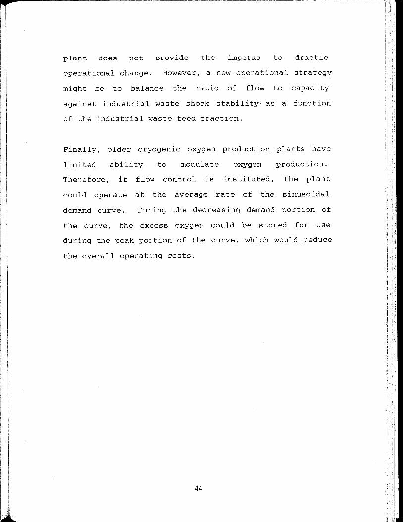
plant does not provide the impetus to drastic

operational change. However, a new operational strategy

might be to balance the ratio of flow to capacity

against industrial waste shock stability as a function

of the industrial waste feed fraction.

Finally, older cryogenic oxygen production plants have

limited ability to modulate oxygen production.

Therefore, if flow control is instituted, the plant

could operate at the average rate of the sinusoidal

demand curve. During the decreasing demand portion of

the curve, the excess oxygen could be stored for use

during the peak portion of the curve, which would reduce

the overall operating costs.

44

i I, I, i I I

i I

:I I

VII REFERENCES

1. Speckhart,F.H.,Green,W.L.,A Guide to Usjng CSMP -

The Contjnuous System Modeling Program. A Program

for Simulating Physical Systems.,Prentice-Hall,Inc.

Englewood Cliffs, New Jersey, 1976

2. Mueller,J.A. ,Mulligan,J.J. ,and DiTora,D.M., "Gas

Transfer Kinetics of Pure Oxygen Systems", Journa.l

of the Env.ironmenta.l Engineering D.ivis.ion,

ASCE,1973,Vol.99,pp.269-282

3. Gaudy,A.F.,Srinivasaraghavan,R.,and Saleh,M.,

"Conceptual Model for Activated Sludge Processes",

Journa.l of the Environmenta.l Eng.ineer.ing D.iv.is.ion,

ASCE,1977,Vol.103,pp.71-85

4. McWhirter,J.K. ,and Vahldieck,N.P.," Oxygenation

Systems Mass Transfer Design Considerations," in

the Activated Sludge Process: Volume 1,

McWhriter,J.R.,ed.,Chemical Rubber Company

Press,Inc.,Cleveland,Ohio,pp.235-260 (1978)

5. Stenstrom,M.K.,and Andrews,J.F.," Real-Time Control

of Activated Sludge Process", Journa.l of t:he

Environmenta.l Eng.ineer.ing Division, ASCE, 1979,

Vol.105, pp.245-260

45

6. Hansen,J.L.,Fiok,A.E.,and Hovious,J.C., 11 Dynamic

Modeling of Industrial Wastewater Treatment Plant

Data 11, Journa.l of t:he N'at:er Po.l.lut:.ion Cont:ro.l

Federat:.ion, Vol. 52, No.7, pp.1965-1975(1980)

7. Clifft,R.C.,Andrews,J.F., 11 Predicting the Dynamics

of Oxygen Utilization in the Activated Sludge

Process", Journa.l of t:he N'at:er Po.l.lut:.ion Cont:ro.l

Federat:.ion, Vol. 53, No.7, pp .1219-1232 ( 1981)

8. Clifft,R.C.,Andrews,J.F.," Gas-Liquid Interactions

in Oxygen Activated Sludge", Journa.l of t:he

Environment:a.l Engineering D.ivis.ion, ASCE, 1986,

Vol~112, pp.61-77

9. Clifft,R.C.,Barnett,M.W. 11 Gas Transfer Kinetics in

Oxygen Activated Sludge", Journa.l of t:he

Env.ironment:a.l Eng.ineer.ing D.iv.is.ion, ASCE, 19 88,

Vol.114, No.2, pp.415-432

10. Stenstrom,M.K. ,Kido,R.F. ,Mulkerin,S.M. 11 Estimating

Oxygen Transfer Capacity of a Full-Scale Pure

Oxygen Activated Sludge Plant 11, Journa.l of t:he

N'at:er Po.l.lut:.ion Cont:ro.l Federat:.ion, Vol. 61, No.2,

pp.208-220(1989)

46

11. Andrews,J.F." Kinetic ModeJs of BioJogical Waste

Treatment Processes," Canale,R.P.,ed.,Interscience

Publishers,New York,pp.S-33 (1971)

12. Weast,R.C.,Handbook of Chemistry and Physics,65th

Edition,Chemical Rubber Company, Cleveland, Ohio,

1985.

13. Snoeyink,V.L.,Jenkins,D.,Water Chemistry,John Wiley

& Sons, New York,1980.

14. Wunderlich,R.,Barry,J.,Greenwood,D.,Carry,C.

"Start-up of a High Purity,Oxygen-Activated Sludge

System at the Los Angeles County Sanitation

Districts' Joint Water Pollution Control Plant",

Journa.l of t:he fllat:er Po.l.lut:.ion Cont:ro.l

Federat:.ion, Vol. 57, No.10, pp.1012-1018(1985)

15. Yunt, F.," Analysis of Surface Aerator Shop

Performance Tests Conducted at the Mixco Test

Facility in Rochester, New York ", County

Sanitation Districts of Los Angeles County,

Internal Report, October 1979

47

I

APPENDIX

A MODEL PARAMETERS

B COMPUTER PROGRAM LISTING

48

SECTION A:

Model Parameters

Muhat = 0.25 hr-1

y = 0.62

Yo21 = 1. 07

Yo22 = 1.42

YNH31 = 0.039

YNH32 = 0.1239

Ksno = 2.5 g/M3

Ks = 50 g/M3

Yco21 = 1. 37

Yco22 = 1. 95

Kn = 0.0127 hr-1

BETA = 0.985

KLaC02 = 0.836KLa02

KLaN2 = 0.943KLa02

THETA = 1.024

BOD5TOU = 0.52

49

SECTION B:

Computer Program Listing

50

MACRO

XJ,SJ,DOJ,DN2J,DCDJ,HIJ,FCDJ,QGJ,PC02J,P02J,PN2J,C02J,N2J,02J, ...

DNH3J,ALKJ=REACT(THETAJ,XOJ,SOJ,DOOJ,DN20J,DCDOJ,HIOJ,QGOJ,C020J,.

N20J,020J,ICXJ,ICSJ,ICDOJ,ICDN2J,ICDCDJ,ICC02J,IC02J,ICN2J,CKLAOJ,

VLJ,TPRESJ,TPRESI,DNH30J,ALKOJ)

********** LIQUID PHASE MASS BALANCES ***************

* CORRECT FLOW FOR PRESSURE CHANGE

QGNJ=QGOJ*TPRESJ/TPRESI

* MICROBIAL MASS BALANCE

DXDT = (XOJ- XJ)/THETAJ + (MUJ- KD*02LIM) * XJ

XJ = INTGRL(ICXJ,DXDT)

* ORGANISM GROWTH RATE

* MUJ = MUHAT*SJ*DOJ/((SJ +KS)*(DOJ+KSDO))

* COMMENT OUT THE ABOVE EXPRESSION FOR MU AND SUBSTITUTE WITH THE

* FOLLOWING EXPRESSION WHICH IS MORE CONVENIENT FOR PREFORMANCE

CALCS.

02LIM=(DOJ/KSDO) I (l.+(DOJ/KSDO))

MUJ =MUHAT*SJ/(SJ+KS)*02LIM

* SUBSTRATE BALANCE

DSDT = (SOJ- SJ)/THETAJ -MUJ*XJ/Y

SJ INTGRL(ICSJ,DSDT)

* AMMONIA BALANCE

DNH3RJ=(YNH32*KD*02LIM + YNH31*MUJ/Y- YNH32*MUJ)*XJ

DDNH3J=(DNH30J-DNH3J)/THETAJ+DNH3RJ

DNH3J=INTGRL(ICNH3J,DDNH3J)

* CALCULATE THE ALKALINITY INCREASE FROM AMMONIA INCREASE

ALKJ=ALKOJ+(DNH3J-DNH30J)/14.E+03

* SET THE MASS TRANSFER COEFFICIENTS FOR NITROGEN AND CARBON

DIOXIDE

* TO THE SOME FRACTION OF THE VALUE FOR OXYGEN

CKLANJ=CKLAOJ*FKLAN2

CKLACJ=CKLAOJ*FKLACO

* DISSOLVED OXYGEN

02UPJ=MUJ*XJ*YP021 + KD*XJ*Y022*02LIM

51

DODT= (DOOJ- DOJ)/THETAJ + SDOJ- 02UPJ

DOJ = INTGRL(ICDOJ,DODT)

* DISSOLVED NITROGEN

DN2DT=(DN20J- DN2J)/THETAJ +SDN2J

DN2J = INTGRL(ICDN2J,DN2DT)

* DISSOLVED C02

*DCDR=MUJ*XJ*YPC021 + KD*XJ*YC022*02LIM

DCDRJ=02UPJ*1.375

DCDDT=(DCDOJ-DCDJ)/THETAJ+SDCDJ + DCDRJ

DCDJ = INTGRL(ICDCDJ,DCDDT)

********** GAS SATURATION CONCENTRATIONS ****************

* OXYGEN

DOSJ=P02J/HE02

* NITROGEN

DN2SJ=PN2J/HEN2

* CARBON DIOXIDE

DCDSJ=PC02J/HEC02

~-----~ --- -~ ----

********** PH AND FRACTION OF DISSOLVED CARBON DIXOIDE WHICH IS

* H2C03 (USE FUNCTIONS TO SIMPLIFY)

FCDJ =FC02(HIJ,CK1,CK2)

HIJ=PHCAL(ALKJ,DCDJ,DNH3J,CK1,CK2,CKW,CKNH3)

************** GAS SIDE BALANCES*************************

* STRIPPING RATES

* C02

SDCDJ=CKLACJ*(DCDSJ- DCDJ*FCDJ)

* DO

SDOJ =CKLAOJ*(DOSJ- DOJ)

* NITROGEN

SDN2J =CKLANJ*(DN2SJ- DN2J)

* VOLUMETRIC GAS PRODUCTION

QGJ=LIMIT(0.,10000., (KFLOW*((VPH20+PC02J+P02J+PN2J) -TPRESJ)))

* C02 BALANCE

C02DT = (QGNJ*C020J- QGJ*C02J)/VG -SDCDJ*VLJ/(VG*MWC02)

C02J = INTGRL(ICC02J,C02DT)

* N2 BALANCE

N2DT = (QGNJ*N20J - QGJ*N2J)/VG -SDN2J*VLJ/(VG*MWN2)

52

N2J = INTGRL(ICN2J,N2DT)

* 02 BALANCE

02DT =(QGNJ*020J- QGJ*02J)/VG -SDOJ*VLJ/(VG*MW02)

02J =INTGRL(IC02J,02DT)

* PARTIAL PRESSURES

* C02

PC02J = C02J*RT

* N2

PN2J = N2J*RT

* 02

P02J = 02J*RT

ENDMAC

**********************************************************

INITIAL

* THIS SECTION DESCRIBES THE INITIAL CONDITIONS AND INPUTS TO THE

* REACTORS.

* * FIRST THE BI.OX PARAMETERS

PARAM MUHAT=0.250, Y=0.62, Y021=1.07,Y022=1.42,YB5TOU=0.52

PARAM YNH31=0.039,YNH32=0.1239

PARAM KSD0=2.50, KS=50., YC021=1.37,YC022=1.95,KD=0.01270,NPRINT=2

* PARAMETERS FOR SLUDGE RECYCLE

PARAM ALKR=5.76E-03,DCDR=120.,DN2R=10.

PARAM DTIME1=0.,DTIME2=100.0,0FFSET=0.,02LAG=O

PARAM MWC02=44.009,MWN2=28.013,MW02=31.998,R=8.2056E-05

* ALPHA AND BETA FACTORS; EFFECTIVE SATURATION DEPT

********* MODIFY FOR COUNTY **************

PARAM

ALPHA1=1.000,ALPHA2=1.000,ALPHA3=1.000,ALPHA4=1.000,BETA=0.985

PARAM CFCONV=0,58858

* RATIOS OF NITROGEN AND C02 KLA'S TO OXYGEN

PARAM FKLAC0=0.836,FKLAN2=0.943,BKLA1=11.875

* CSD'S KLAS FROM CLEAN WATER TANK TEST

PARAM BKLA2=6.208,BKLA3=6.208,BKLA4=7.767

* FIT 02 FEED RATE TO MATCH ORIGINAL OPERATIONAL PERFORMANCE

PARAM 02ERR=1.08

* OPERATIONAL SIMULATION AND OPTIMIZATION PARAMETERS

53

PARAM MGDMOD=l.O

PARAM FPMOD=l.O

PARAM KLAMOD=l.O

PARAM BOOST=O.O

FEDFLX=(l+BOOST*SIN(0.2618*TIME))

PARAM DOSP=6.0,KERR=l.O,KINTER=l.O

DOERR=(DOSP-D04)

GASMOD=DOERR*KERR+KINTER*INTGRL(O.O,DOERR)

* SET THE CONTROLLER PARAMETERS

PARAM RSETS=O.,RSETI=O.O,SRTSP=7.,R02GP=O.,R02GI=O.O

* TOTAL PRESSURES. LET THEM VARY BY 2 INCHES

PARAM TPRES1=1.006,TPRES2=1.0045,TPRES0=1.006

PARAM TPRES3=1.0030,TPRES4=1.0015

** INITIAL CONDITIONS

PARAM ICS1=120.,ICD01=11.0,ICNH3J=24.0

PARAM ICS2=90.,ICD02=16.4



* INITIAL PURITY PROFILES IN FRACTIONS (SAME AS PARTIAL PRESSURE)

PARAM FP021=.905,FP022=0.7202,FP023=0.5888,FP024=0.4106

PARAM FPC021=0.0l,FPC022=0.0l,FPC023=0.01,FPC024=0.01

PARAM ICPH1=7.5,ICPH2=7.5,ICPH3=7.5,ICPH4=7.5

* INLET GAS PURITY (% 02) AND OXYGEN FLOW IN TONS PER DAY.

PARAM ZWSCFM=0.056

* CHECK INTO CSD'S WATTAGE DRAW PER STAGE

PARAM ZWM1=286.0,ZWM2=183.0,ZWM3=176.0,ZWM4=207.0

** INFLUENT PARAMETERS

PARAM BOD5IN=l53.,PH0=7.6,DOO=O.,DNH3I=l3.5,XPEFF=O.

PARAM ACAC03=275.

PARAM QMGDA=63.,QRRAT=0.35,NBASIN=l

QMGDI=QMGDA*MGDMOD

* LIQUID VOLUMES

PARAM VLCF1=175781.,VLCF2=175781.,VLCF3=175781.,VLCF4=175781.

* GAS VOLUMES

PARAM KFLOW=80000.

PARAM VGCF1=58594.,VGCF2=58594.,VGCF3=58594.,VGCF4=58594.

54

* HEAD SPACE VOLUME

FIXED NPRINT

** NOW THE FUNCTIONS FOR ION PRODUCTS OF WATER, CARBONIC ACID,

*AMMONIA,

* AND VAPOR PRESSURE OF WATER.

FUNCTION

FPKW=(0,,14.944), (5.,14.734), (10.,14.535), (15.,14.346), ...

(20.,14.167)' (25.,13.996)' (30.,13.833)' (35.,13.680)' (40.,13.535)'.

(50.,13.262)

* AMMONIA

FUNCTION FPKNH3=(0.,10.081), (5.,9.904), (15.,9.564), (20.,9.4), ...

(25.,9.245)' (30.,,9.093)' (35.,8.947)' (40.,8.805)' (50.,8.539)

* CARBON DIOXIDE PK1

FUNCTION

FPK1 = ( 0 . , 6 . 58) , ( 1 0 . , 6 . 4 6) , ( 15 . , 6 . 4 2) , ( 2 0 . , 6 . 3 8) , ( 2 5 . , 6 . 3 5) , ...

(30.,6.34), (35.,6.332)' (40.,6.325)' (45.,6.3215)' (50.,6.320)

* CARBON DIOXIDE PK2

FUNCTION FPK2= (0., 10. 63), (10., 10. 49), (15., 10. 43), (25., 10. 33), ...

(40.,10.22)' (50.,10.17)

* VAPOR PRESSURE OF H20 IN MM HG

FUNCTION FVPH2 0= ( 0 . , 4 . 57 9) , ( 5 . , 6 . 54 3 ) , ( 1 0 . , 9 . 2 0 9) , ( 15 . , 12 . 7 8 8) , ...

(20. ,17 .535)' (25. ,23 .756)' (30. ,31.824)' (35. ,41.175)' ...

(40.,55.324)' (50.,92.51)

* SET THE MEASURED VARIABLES FOR THE INITIAL SECTION

** LOAD CARSON DATA INTO FILES FOR COMPARISON TO MODEL

P021D=GDATA(TIME,1)

P022D=GDATA(TIME,2)

P023D=GDATA(TIME,3)

P024D=GDATA(TIME,4)

D01D=GDATA(TIME,5)

D02D=GDATA(TIME,6)

D03D=GDATA(TIME,7)

D04D=GDATA(TIME,8)

FPUR02=GDATA(TIME,9)*FPMOD

55

* TGASM1=GDATA(TIME,10)

* TGASMU=TGASM1*02ERR

TGASMU=0.9*QMGD+GASMOD

QMGD=GDATA(TIME,11)*MGDMOD*FEDFLX

TEMP=AFGEN(TEMPF,TIME)

BOD5IN=GDATA(TIME,12)

BOD50D=GDATA(TIME,13)

XSETA=GDATA(TIME,18) -OFFSET

** LATER USE OFFSET TO ADJUST MODEL WASTE RATE TO MATCH MLVSS

***** CALCULATE THE CONSTANTS

PK1=NLFGEN(FPK1,TEMP)

CK1=1./(10**PK1)

PK2=NLFGEN(FPK2,TEMP)

CK2=1./(10**PK2)

PKNH3=PKW-NLFGEN(FPKNH3,TEMP)

CKNH3=1./(10**PKNH3)

PKW=NLFGEN(FPKW,TEMP)

CKW=1./(10**PKW)

* WATER VAPOR PRESSURE (CONVERT TO ATMOSHPHERES)

VPH20=NLFGEN(FVPH20,TEMP)/760.

***** HENRY'S LAW CONSTANTS.

* OXYGEN (* 10 E-04 )

FUNCTION FH02=(0.,2.5410), (5.,2.903), (10.,3.279), (15.,3.66),

(20,,4,052) 1 (25,,4,434) f (30,,4,869) f (35,,5,07) 1 (40,,5,35)

* NITROG (* 10E-04 )

FUNCTION

FHN2 = ( 0 . I 5 . 2 9 ) I ( 5 . I 5 . 9 7 ) I ( 1 0 . I 6 . 6 8 ) I ( 15 . I 7 . 3 8 ) I ( 2 0 . I 8 . 0 4 ) I • • •

(25,,8,65) 1 (30,,9,24) 1 (35,,9,85) f (40,,10,4) 1 (50,,1.13)

* CARBON DIOXIDE (* 10 E-03 )

FUNCTION FHC02=(0.,0.728) I (5.,0.876) I (10.,1.04) I (15.,1.22) I •••

(20,,1,42) I (25,,1,64) 1 (30,,1.86) f (35,,2,09) f (40,,2,33) 1 (50,,2,83)

***** CALCULATE THE CONSTANTS INCLUDING THE MW OF EACH SPECIES AND

**

*** THE MOLE FRACTION OF WATER

HE02=NLFGEN(FH02,TEMP)/(55555.*MW02*1.E-04*BETA)

56

HEN2=NLFGEN(FHN2,TEMP)/(55555.*MWN2*1.E-04*BETA)

HEC02=NLFGEN(FHC02,TEMP)/(55555.*MWC02*1.E-03*BETA)

***** GAS TRANSFER COEFFICIENTS

* FIRST STAGE

* FUNCTION FKLA1 PREVIOUSLY A FUNCTION OF GAS RECIRCULATION RATES

*** TEMPERATURE FOR THE FIRST TEST

FUNCTION

TEMPF= (0., 27. 0) , (8., 27. 0) , (32., 27. 0), (56. I 27. 0) I (80., 27. 0) , ...

(104,,27,0) 1 (128,,27,0) 1 (152,,27,0) 1 (168,,27,0) 1 (200,,27,0) 1 ,,,

(300.127 .0), (408. ,27 .0)

**** CALCULATE THE COEFFICIENTS

* CALCULATE THE VALUE OF R * T

RT=R*(TEMP+273.15)

* CALCULATE THE INLET HYDROGEN ION CONCENTRATION FROM PHO

HI0=1./(10**PHO)

* CALCULATE THE INLET AMMONIA CONCENTRATION IN G/MOLES

* NH3I=CNH3I/14.E+03

* CONVERT THE VOLUMES TO M**3 AND CALCULATE THETAS. FOR THE

Q=QMGDI*1.E+06*0.003875/(24.*NBASIN)

QR=QRRAT*Q

QT=Q+QR

XR=XSETA*QT/QR

VL1=VLCF1*0.02832

VL2=VLCF2*0.02832

VL3=VLCF3*0.02832

VL4=VLCF4*0.02832

VG=VGCF1*0.02832

THETA1=VL1/(Q+QR)

THETA2=VL2/(Q+QR)

THETA3=VL3/(Q+QR)

THETA4=VL4/(Q+QR)

ALKI=ACAC03/(50.E+03)

* CALCULATE THE INITIAL PARTIAL NITROGEN PRESSURE BY DIFFERENCE

* INDICATED AS %

FPN21=TPRES1-VPH20-FP021-FPC021


57



* INITIAL GAS HEADSPACE CONCENTRATIONS FROM ABOVE CONVERTED TO

* MOLES

IC021=TPRES1*FP021/RT

ICN21=TPRES1*FPN21/RT

ICC021=TPRES1*FPC021/RT










* INITIAL MLVSS. CONCENTRATIONS

ICXS=XR*QR/(QR+Q)

ICXl=ICXS

ICX2=ICXS

ICX3=ICXS

ICX4=ICXS

* CALCULATE THE INLET DISSOLVED GAS CONCENTRATIONS

DN2I=0.791/HEN2

DOI=O.

DCDI=(ALKI- (DNH3I/14.E+03)/(1. + HIO * CKNH3/CKW)) *

MWC02*1.E+03

* INITIAL PH CALCULATIONS

HI1=10**(-ICPH1)

HI2=10**(-ICPH2)

HI3=10**(-ICPH3)

HI4=10**(-ICPH4)

* INITIAL CONDITIONS FOR DISSOLVED GASSES. CALCULATE FROM

* PARTIAL PRESSURES. ASSUME SATURATION

ICDCD1=TPRES1*FPC021/(HEC02*FC02(HI1,CK1,CK2))

ICDN21=TPRES1*FPN21/HEN2

58

ICDCD2=TPRES2*FPC022/(HEC02*FC02(HI2 1 CK1 1 CK2))






* CALCULATE THE INLET VOLUMETRIC GAS FLOW RATE

TGASB=TGASMU*2000./(24.*NBASIN)

QGO=TGASB*RT*454./(MW02*(TPRES1-VPH20))+TGASB*(l.

FPUR02)/FPUR02 *RT*454./(MWN2*(TPRES1-VPH20))

020=(TPRES1-VPH20)*FPUR02/RT

N20=(TPRES1-VPH20)*(1.-FPUR02)/RT

QGOCF=QGO*CFCONV

C020=0.

* CALCULATE THE FOLLOWING COMBINATIONS OF PARAMETERS TO IMPROVE

* SPEED.

YP021=(1.-Y)*Y021/Y

YPC021=(1.-Y)*YC021/Y

YPNH3l=YNH32-YNH31

* CONVERSION FACTOR FOR GLOBAL BALANCES

CFTON=NBASIN*24./(454.*2000.)

* CALCULATE THE LEAK FLOWS

** QLKl= NOT FOR CSD

SOI=BOD5IN/YB5TOU

* CALCULATE INITIAL CONDITIONS FOR SRT AND FMR

SODIFF=(Q+QR)*(SOI-ICS4)*CFTON

SMASS=NBASIN*(ICXl*VLl+ICX2*VL2+ICX3*VL3+ICX4*VL4)/9.098E+05

XMDIFF=LIMIT (0. 004 I 1000. I ( (ICX4* (Q+QR) -QR*XR) *CFTON))

**************************************************************

DYNAMIC

NOSORT

CALL DEBUG(NPRINT 1 DTIME1)

CALL DEBUG(NPRINT 1 DTIME2)

SORT

PROCEDURE DOlD 1 D02D 1 D03D 1 D04D 1 P021DI ...

P022D1

P023D 1 P024D 1 TGASM1 1 FPUR02 1 TEMP 1 BOD5IN=INDATA(TIME)

59

* IF(KEEP.NE.l) GOTO 90

P021D=GDATA(TIME,l)

P022D=GDATA(TIME,2)

P023D=GDATA(TIME,3)

P024D=GDATA(TIME,4)

D01D=GDATA(TIME,5)

D02D=GDATA(TIME,6)

D03D=GDATA(TIME,7)

D04D=GDATA(TIME,8)

FPUR02=GDATA(TIME,9)*FPMOD

* TGASMl=GDATA((TIME-02LAG) ,10)*02ERR

TGASM1=0.9*QMGD+GASMOD

QMGD=GDATA(TIME,ll)*MGDMOD*FEDFLX

TEMP=AFGEN(TEMPF,TIME)

BOD5IN=GDATA(TIME,12)

BOD50D=GDATA(TIME,13)

XSETA=GDATA(TIME,18) -OFFSET

90 CONTINUE

END PROCEDURE

DOERR=(DOSP-D04)

GASMOD=DOERR*KERR+KINTER*INTGRL(O.O,DOERR)

TFAC=l.024**(TEMP-20.)

RT=R*(TEMP+273.15)

TGASB=TGASMU *2000./(24.*NBASIN)

QGO=TGASB*RT*454./(MW02* (TPRES1-VPH20))+TGASB* (1.

FPUR02)/FPUR02 *RT*454./(MWN2* (TPRES1-VPH20))

020=(TPRES1-VPH20)*FPUR02/RT

N20=(TPRES1-VPH20)*(1.-FPUR02)/RT

QGOA=QGO

* INFLUENT PARAMTERS

FEDFLX=(l+BOOST*SIN(0.2618*TIME))

Q=QMGD*l.E+06*0.003875/(24.*NBASIN)

* QR=QRRAT*Q

QT=Q+QR

THETAl=VLl/(Q+QR)

THETA2=VL2/(Q+QR)

60

THETA3=VL3/(Q+QR)

THETA4=VL4/(Q+QR)

SOI=BOD5IN/YB5TOU

DCDI=(ALKI- (DNH3I/14.E+03)/(1. + HIO * CKNH3/CKW)) *

MWC02*1.E+03

* CALCULATE THE RESULTS OF MIXING RECYCLE AND INFLUENT FLOWS. MOVE

* IT TO THE DYNAMIC SECTION FOR TIME VARYING FLOW RATE.

PROCEDURE SO,DNH30,ALKO,DCDO,DN20,SOA,XOA = INPUT(Q,QR,QT)

XO=(Q*XPEFF+QR*XR)/QT

SO=(Q*SOI+QR*S4)/QT

DNH30=(Q*DNH3I+QR*DNH31)/QT

ALKO=(Q*ALKI+QR*ALKR)/QT

DCDO=(Q*DCDI+QR*DCDR)/QT

DN20=(Q*DN2I+QR*DN2R)/QT

XOA=XO

SOA=SO

END PROCEDURE

* CKLA2L=NLFGEN(FKLA2,GAS2) --- KLAAS A FUNCTION OF GAS

* RECIRULATION RATIO NOT APPLICABLE TO CARSON

CKLAl=BKLAl*TFAC*ALPHAl*KLAMOD

CKLA2=BKLA2*TFAC*ALPHA2*KLAMOD



Xl,Sl,D01,DN21,DCD1,HI1,FCD1,QG1,PC021,P021,PN21,C021,N21,021, ...

DNH31,ALK1=REACT(THETA1,XOA,SOA,DOO,DN20,DCDO,HIO,QGOA,C020,N20, ..

020,ICX1,ICS1,ICD01,ICDN21,ICDCD1,ICC021,IC021,ICN21,CKLA1, ...

VL1,TPRES1,TPRESO,DNH30,ALKO)

* MIX THE FLOWS FOR SLUDGE REAERATION. PROCEDURE DROPPED FOR CSD

** STAGE #2 **

X2,S2,D02,DN22,DCD2,HI2,FCD2,QG2,PC022,P022,PN22,C022,N22,022, .. .

DNH32,ALK2=REACT(THETA2,Xl,Sl,D01,DN21,DCD1,HI1,QG1,C021,N21, .. .

021,ICX2,ICS2,ICD02,ICDN22,ICDCD2,ICC022,IC022,ICN22,CKLA2, .. .

VL2,TPRES2,TPRES1,DNH31,ALK1)

** STAGE #3 **

X3,S3,D03,DN23,DCD3,HI3,FCD3,QG3,PC023,P023,PN23,C023,N23,023, ...

61

DNH33 1 ALK3=REACT(THETA3 1 X2 1 S2 1 D02 1 DN22 1 DCD2 1 HI2 1 QG2 1 C022 1 N22 1 •••

022 1 ICX3 1 ICS3 1 ICD03 1 ICDN23 1 ICDCD3 1 ICC023 1 IC023 1 ICN23 1 CKLA3 1 •••

VL3 1 TPRES3 1 TPRES2 1 DNH32 1 ALK2)

** STAGE #4 **

X4 1 S4 1 D04 1 DN24 1 DCD4 1 HI4 1 FCD4 1 QG4 1 PC024 1 P024 1 PN24 1 C024 1 N24 1 024 1 •••

DNH34 1 ALK4=REACT(THETA4 1 X3 1 S3 1 D03 1 DN23 1 DCD3 1 HI3 1 QG3 1 C023 1 N23 1 •••

023 1 ICX4,ICS4 1 ICD04 1 ICDN24,ICDCD4 1 ICC024 1 IC024 1 ICN24 1 CKLA4 1 •••

VL4 1 TPRES4 1 TPRES3 1 DNH33 1 ALK3)

*********************************************************

BOD50C=S4*YB5TOU

PH1=-ALOG10(LIMIT(l.E-14 1 1. 1 HI1))




SR=S4

NO SORT

* THIS SECTION CONTROLS THE SLUDGE AGE

* CONSIG=INSW( (TIME-3.) I 0. I (SRTSP-SRT))

* XSET1=RSETS*(CONSIG)+RSETI*INTGRL(0. 1 CONSIG)+XSETA

XSET=LIMIT( 500. 1 3200. 1 XSETA)

XR=QT/QR*XSET

* CONP=LIMIT(0. 1 1.0 1 PUTILU)

TGASMU=TGASMl

SORT

* CALCULATE THE GLOBAL BALANCE INFORMATION AFTER STEADY-STATE

* HAS BEEN REACHED. MOVE THIS SECTION TO TERMINAL TO INCREASE

SPEED.

MLSS=(Xl+X2+X3+X4)/4

XMDIFF=LIMIT (0. 004 I 1000. I ( (X4* (Q+QR) -QR*XR) *CFTON))

SODIFF=(Q+QR)*(SO-S4)*CFTON

N2MIN=(QGO*N20*MWN2+Q*DN2I+QR*DN2R)*CFTON

02MIN=QG0*020*MW02*CFTON

C02MIN=(C020*MWC02+Q*DCDI+QR*DCDR)*CFTON

02MOUT=(QG4*024*MW02+(Q+QR)*D04)*CFTON

C02MOU=(QG4*C021*MWC02+(Q+QR)*DCD1)*CFTON

N2MOUT=(QG4*N21*MWN2+(Q+QR)*DN24)*CFTON

62

02UTIL=02MIN-02MOUT

PUTIL=02UTIL/02MIN

02MOUC=QG4*024*MW02*CFTON

02UTIU=02MIN-02MOUC

PUTILU=02UTIU/02MIN

02CONS=02UTIL/SODIFF

C02PRO=(C02MOU-C02MIN)/SODIFF

C02CHK=SODIFF*(l.-Y)*YC02l+(SODIFF*Y-XMDIFF)*YC022

SMASS=NBASIN* (Xl*VLl+X2*VL2+X3*VL3+X4*VL4)/9.098E+05

ERRDOl=ABS(DOl-DOlD)

ERRD02=ABS(D02-D02D)



ERRPOl=ABS(P021-P021D)

ERRP02=ABS(P022-P022D)

ERRP03=ABS(P023-P023D)

ERRP04=ABS(P.024-P024D)

ERRDOT=ERRDOl+ERRD02+ERRD03+ERRD04

ERRPOT=ERRPOl+ERRP02+ERRP03+ERRP04

IERRDO=INTGRL(O.,ERRDOT)

IERRPO=INTGRL(O.,ERRPOT)

* ENERGY CALCULATIONS

* MIXERS-- USE THE POWERS MEASURED IN THE GILBERT REPORT

ZWMIX=NBASIN* (ZWM1+ZWM2+ZWM3+ZWM4)

* GAST=(GASl)*NBASIN

* ZWBLOW=ZWSCFM*GAST

ZWALL=ZWBLOW+ZWMIX

* ZWSl=NBASIN* (ZWMl)

* POWER WEIGHTED DO, PURITY, AND ALPHA

DOAVI=INTGRL(O., ((DOl*ZWMl+D02*ZWM2+D03*ZWM3+D04*ZWM4)/ZWALL))

P02AVI=INTGRL(O., ((P02l*ZWMl+P022*ZWM2+P023*ZWM3+P024*ZWM4)/ZWALL)

ALPHAI=INTGRL(O., ((ALPHAl*ZWMl+ALPHA2*ZWM2+ALPHA3*ZWM3+ALPHA4* ...

ZWM4) /ZWALL))

* 02 CONSUMTION BY STAGE

02COI1=INTGRL(O., (QGOA*020-QG1*02l)*CFTON*MW02)

63

02COI2=INTGRL (0., (QG1*021-QG2*022) *CFTON*MW02)

02COI3=INTGRL (0., (QG2*022 -QG3*023) *CFTON*MW02)

02COI4=INTGRL (0., (QG3*023 -QG4*024) *CFTON*MW02)

02COI5=INTGRL (0., (QGOA*020-QG4*024) *CFTON*MW02)

* 02 PURITY AVERAGE

PUTAVI=INTGRL(O.,PUTILU)

DOli=INTGRL(O.,DOl)

D02I=INTGRL(O.,D02)

D03I=INTGRL(O.,D03)

D04I=INTGRL(O.,D04)

P021I=INTGRL(O.,P021)




ENDT=TIME

NO SORT

FMR=YB5TOU*(SODIFF/SMASS)

SRT=LIMIT (0., 100., (SMASS/XMDIFF))

TERMINAL

* POWER WEIGHTED DO, PURITY, AND ALPHA

DOAVG=DOAVI/ENDT

P02AVG=P02AVI/ENDT

ALPHAA=ALPHAI/ENDT

* 02 CONSUMPTION BY STAGE

02CON1=02COI1/ENDT

02CON2=02COI2/ENDT

02CON3=02COI3/ENDT

02CON4=02COI4/ENDT

* 02 TOTAL CONSUMPTION

02CON5=02COI5/ENDT

* 02 PURITY AS A FUNCTION OF TIME

PUTAVE=PUTAVI/ENDT

DOlA=DOli/ENDT

D02A=D02I/ENDT

D03A=D03I/ENDT

D04A=D04I/ENDT

64

P021A=P021I/ENDT

P022A=P022I/ENDT

P023A=P023I/ENDT

P024A=P024I/ENDT

* WRITE OUT THE RESULTS WITH FORTRAN WRITES

WRITE(6,1004)

1004

KW')

1005

FORMAT (' STAGE RECIRCULATION DO P02

WRITE(6,1005)

FORMAT(' (NO) (SCFM / STAGE) (MG/L) (FRAC)

WRITE(6,1010) GAS1,D01A,P021A,02CON1,PH1,ZWM1

WRITE (6, 1020) GAS2,D02A,P022A,02CON2,PH2,ZWM2

WRITE(6,1030) GAS3,D03A,P023A,02CON3,PH3,ZWM3

WRITE (6, 1040) . GAS4, D04A, P024A, 02CON4, PH4, ZWM4

WRITE(6,1050) GAST,DOAVG,P02AVG,02CON5,ZWALL

02 UPTAKE PH

(TON/DAY) ' )

1010 FORMAT(1X,' 1 ' 8X,F5.0,4X,F6.2,4X,F5.2,F8.1,4X,F3.1,F6.0)




1050 FORMAT(/,' T' 6X,F7.0,4X,F6.2,4X,F5.2,F8.1,6X,F7.0)

WRITE(6,1060) PUTAVE,ALPHAA,NBASIN

1060 FORMAT(//,' FRACTION OXYGEN UTILIZATION=' ,F5.3,/, .. .

/,' POWER WEIGHTED ALPHA FACTOR=' ,F5.3,/, .. .

/,' NUMBER OF BASINS IN SERVICE=' ,F4.0,///)

WRITE(6,1070)

1070 FORMAT('1')

METHOD STIFF

PRINT

X1,S1,DNH31,D01,DN21,DCD1,PH1,ALK1,FCD1,QG1,PC021,P021,PN21, .. .




XR,XSET,SRT,FMR

OUTPUT

QMGD,BOD5IN,BOD50D,BOD50C,D01,D01D,D02,D02D,D03,D03D,D04, ...

D04D,P021,P021D,P022,P022D,P023,P023D,P024,P024D,S1,S4,MLSS, ...

65

FMR,SRT;PUTIL,02CONS,XMDIFF,ERRD01,ERRD02,ERRD03,ERRD04,ERRDOT, ...

IERRDO,ERRP01,ERRP02,ERRP03,ERRP04,ERRPOT,IERRPO,PUTILU

OUTPUT D01,D02,D03,D04,D01D,D02D,D03D,D04D,TGASM1

OUTPUT P021,P022,P023,P024,P021D,P022D,P023D,P024D,QGO

TIMER FINTIM=100.0,PRDEL=24.,0UTDEL=4.,DELMIN=1.68E-06

END

STOP

FUNCTION SDIV(A,B)

C .. THIS FUNCTION GIVES YOU A "SAFE" DIVISION

SDIV=-1.

IF(ABS(B) .GT.1.E-20) SDIV=A/B

RETURN

END

FUNCTION PHCAL(ALK,C02,CNH3,CK1,CK2,CKW,CKNH3)

C .. THIS FUNCTION CALCULATES THE PH OF A DILUTE SOLUTION IN A

CLOSED

C BIOX REACTOR. THE CALCULATION IS IMPLICIT

REAL*B DK1,DK2,DC02,DPH,DNH3,DALK,B,C,ZGESS,DKNH3

C .. SET THE FIRST GUESS EQUAL TO THE OLD PH

ZGESS=1.D-06

C .. CONVERT THE SINGLE PRECISION ARGS TO DOUBLE PRECISION

DK1=CK1

DK2=CK2

DKW=CKW

C .. ALSO CONVERT C02 AND NH3 TO MOLAR CONCENTRATION.

DC02=C02/44009.

DALK=ALK

DKNH3=CKNH3

DNH3=CNH3/14.E+03

C .. QUADRATIC COEFFICIENTS

B=DALK-DNH3/(1.+DPH*DKNH3/DKW)

ITER=O

10 C=-DKW- (DK1 + 2 .DO * DK1*DK2/ZGESS) *DC02

C . . CALC THE PH

DPH= (-B+DSQRT(B**2 - 4.DO*C))/2.D+OO

IF(DABS(DPH-ZGESS) .GT.1.D-12) GOTO 20

66

C .. NORMAL CONVERGENCE

PHCAL=DPH

RETURN

20 IF(ITER.GT.10 ) GOTO 30

ZGESS=DPH

B=DALK-DNH3/(1.+DPH*DKNH3/DKW)

TTER=ITER+l

GOTO 10

C .. NO CONVERGENCE

30 WRITE(6,1000) ZGESS,DPH,ITER

1000 FORMAT(' NON CONVERGENCE IN PH CALCULATION.',/,

1 1X,' EXECUTION STOPPING',/,' FINAL GUESS FOR PH=' ,D17.6,

2 /,' FINAL CALC FOR PH=' ,D17.6,/,' ITERATION NUMBER=' ,I5)

PHCAL=DPH

RETURN

END

FUNCTION FC02(PH,CK1,CK2)

C .. THIS FUNCTION CALCULATES THE FRACTION OF THE TOTAL CARBON

WHICH

C IS IN THE H2C03 FORM.

REAL*8 DK1,DK2,DPH

C .. CONVERT TO DOUBLE PRECISION FOR THE CALCULATION

DK1=CK1

DK2=CK2

DPH=PH

FC02=1.D+O/((DPH*DK1*DK2/DPH+DK1)/DPH+1.DO)

RETURN

END

FUNCTION GDATA(TIM,ITYPE)

REAL*4 MLFGEN,MLSS(lO)

DIMENSION TIME(85) ,TF1(85) ,TF2(85) ,TF3(85) ,TF4(85),

1GP1 (85) , GP2 (85) , GP3 (85) , GP4 (85) , DOl (85) , D02 (85) , D03 (85) ,

2D04 (85) ,02FPUR(85) ,02FTON(85) ,QMGD(85) ,020TON(85) ,02VENT(85)

DIMENSION TIME2(85) ,QMGD2(10) ,BODIN(10) ,BODOUT(lO) ,RAS1(10),

1RAS2(10) ,CODIN(lO) ,CODOUT(lO) ,WAS(lO)

DIMENSION TIME3(7) ,XM1(7) ,XM2(7) ,XM3 (7) ,XM4(7) ,TIME4(85)

67

DIMENSION AX1(5) 1 AX2(5) 1 AX3(5) 1 AX4(5) 1 AX5(5) 1 AX6(5) 1 AX7 (5) 1

1AX8(5) IAX9(5) IAX10(5) IAX11(5) IAX12(5) IAX13(5) IAX14(5) IAX15(5) I

2AX16(5) 1 AX17 (5) 1 AX18(5) 1 AX19(5) 1 AX20(5) 1 AX21(5) 1 AX22(5)

DATA AXl /5*0./ 1 AX2 /5*0./ 1 AX3 /5*0./ 1 AX4 /5*0./ 1 AX5 /5*0./ 1

1AX6 /5*0./ 1 AX7 /5*0./ 1 AX8 /5*0./ 1 AX9 /5*0./ 1 AX10 /5*0./ 1

2AX11 /5*0./ 1 AX12 /5*0./ 1 AX13 /5*0./ 1 AX14 /5*0./ 1 AX15/5*0./ 1

2AX16 /5*0./ 1 AX17 /5*0./ 1 AX18 /5*0./ 1 AX19 /5*0./ 1 AX20/5*0./ 1

3AX21/5*0./ 1 AX22/5*0/ 1 JUMP/0/

IF (JUMP.GT.O) GOTO 25

DO 10 I=1 1 8

READ(l6 1 * 1 END=15)

TIME(I) 1 CODIN(I) 1 CODOUT(I) 1 BODIN(I) 1 BODOUT(I)

10 N=I

15 CONTINUE

DO 16 I=l 1 200

READ (17 I *,1 END=17)

TIME2(I) 1 02FTON(I) 1 02VENT(I) 1 020TON(I) 1 02FPUR(I)

16 N2=I

17 CONTINUE

N3=8

DO 18 I=l 1 N3

READ(18 1 * 1 END=19)

TIME3(I) IXMl(I) IXM2(I) IXM3(I) IXM4(I) IRASl(I) I

1RAS2(I) 1 MLSS(I) 1 QMGD(I)

18 N4=I

19 CONTINUE

DO 20 I=1 1 200

READ(20 1 * 1 END=21)

TIME4 (I) I DOl (I) I D02 (I) I D03 (I) I D04 (I) I GP1 (I) I

1GP2 (I) I GP3 (I) I GP4 (I)

20 N5=I

C .. CONVERT THE GAS PERCENTS TO GAS FRACTIONS

21 DO 23 I=l 1 N5

GPl(I)=GPl(I)/100.

GP2(I)=GP2(I)/100.

68

GP3(I)=GP3(I)/100.

23 GP4(I)=GP4(I)/100.

C.. CONVERT OXYGEN FLOW RATES TO GAS FLOW RATES

DO 24 I=1,N2

02FPUR(I)=02FPUR(I)/100.

020TON(I)=020TON(I)/1004.

24 02FTON(I)=02FTON(I)/02FPUR(I)

JUMP=1

25 GOT0(70,80,90,100,110,120,130,140,150,160,170,

1180,190,200,210,220,230,240,250,260,270,280), ITYPE

70 GDATA=MLFGEN(AX1,N5,TIM,TIME4,GP1,56)

GOTO 950


GOTO 950


GOTO 950


GOTO 950

110 GDATA=MLFGEN(AX5,N5,TIM,TIME4,D01,56)

GOTO 950


GOTO 950


GOTO 950


GOTO 950

150 GDATA=MLFGEN(AX9,N2,TIM,TIME2,02FPUR,85)

GOTO 950

160 GDATA=MLFGEN(AX10,N2,TIM,TIME2,02FTON,85)

GOTO 950

170 GDATA=MLFGEN(AX11,N3,TIM,TIME3,QMGD,8)

GOTO 950

180 GDATA=MLFGEN(AX12,N,TIM,TIME,BODIN,8)

GOTO 950

190 GDATA=MLFGEN(AX13,N,TIM,TIME,BODOUT,8)

GOTO 950

69

200 GDATA=MLFGEN(AX14,N3,TIM,TIME3,RAS1,8)

GOTO 950

210 GDATA=MLFGEN(AX15,N3,TIM,TIME3,RAS2,8)

GOTO 950

220 GDATA=MLFGEN(AX16,N,TIM,TIME,CODIN,8)

GOTO 950

230 GDATA=MLFGEN(AX17,N,TIM,TIME,CODOUT,8)

GOTO 950

240 GDATA=MLFGEN(AX18,N3,TIM,TIME3,MLSS,8)

GOTO 950

250 GDATA=MLFGEN(AX19,N3,TIM,TIME3,MX1,8)

GOTO 950


GOTO 950


GOTO 950


950 RETURN

END

FUNCTION MLFGEN(AX,N,X,ARRX,ARRY,M)

C*************************************************************

C .. THIS FUNCTION GENERATES AN ARBITRARY FUNCTION DEFINED BY PAIRS

OF

C DATA POINTS CONTAINED IN THE ARRAIES ARRX AND ARRY, WITH THE

C NUMBER OF POINTS = N.

C NOTE THAT THE FUNCTION CHECKS FOR PROPER DATA ENTRY ON THE

FIRST

C CALL, AND CHECKS TO SEE IF X IS IN THE RANGE DEFINED IN THE

DATA

C ARRAY. QUADRADIC INTERPOLATION IS USED.

C*************************************************************

REAL*4 MLFGEN

DIMENSION ARRX(M) ,AX(5) ,ARRY(M)

C .. CHECK FOR INITIAL ENTRY

NW=6

IF(AX(1)) 10,10,90

70

10 AX(1)=1

IF(N-2) 20,20,30

20 WRITE(NW,1000) N

1000 FORMAT(//,' LESS THAN THREE DATA POINTS (' ,I6,

1' WERE SUPPLIED FOR AN MLFGEN FUNCTION',//,

2' EXECUTION TERMINATING')

STOP 20

30 AX(4)=0

C .. CHECK TO SEE IF THE DATA WAS ENTERED CORRECTLY IN ASCENDING

ORDER

DO 40 I=2,N

IF(ARRX(I-1) .GT.ARRX(I)) GOTO 50

40 CONTINUE

GOTO 60

50 K=I-1

WRITE(NW,1010) I,ARRX(I) ,K,ARRX(K)

1010 FORMAT(//,' THE INDEPENDENT VARIABLE FOR A MLFGEN FUNCTION

HAS '

1'NOT BEEN',/,' ENTERED IN ASCENDING ORDER',/,' THE' ,I3,'TH

POINT='

2,2X,E17.6,2X,'WHILE THE' ,I3,'TH POINT=' ,2X,E17.6,/,'

EXECUTION TER

3MINATING')

STOP 30

60 AX(3)=0.

IF(X.LT.ARRX(1)) AX(3)=-1.

IF(X.GT.ARRX(N)) AX(3)=1.

IF(AX(3)) 70,80,70

70 WRITE(NW,1020) X,ARRX(1) ,ARRX(N)

1020 FORMAT(' THE INITIAL ENTRY TO A MLFGEN FUNCTION IS OUT OF

RANGE', 1/,

1/,' THE VALUE OF THE INDEPENDENT VARIABLE IS' ,E17.6,' WHILE

THE',

2/,' MINIMUM VALUE OF THE FUNCTION IS' ,E17.6, ' AND THE

MAXIMUM' I

3/,' VALUE OF THE FUNCTION IS' ,E17.6)

71

IF(AX(3)) 240,80,210

80 AX(2)=1

C .. NORMAL ENTRY FOR MLFGEN

90 IF(X-ARRX(1)) 220,100,110

100 AX(2)=1

AX(4)=0

MLFGEN=ARRY(1)

GOTO 300

110 IF(X-ARRX(N)) 120,115,190

115 AX (2) =N

AX(4)=0

MLFGEN=ARRY(N)

GOTO 300

120 I=IFIX(AX(2)+0.5)

130 IF(X.LT.ARRX(I)) GOTO 140

I=I+1

IF(I.GT.N) GOTO 190

GOTO 130

140 I=I-1

IF(I.LT.1) GOTO 220

150 IF(X.GE.ARRX(I)) GOTO 160

GOTO 140

160 I=I+1

IF(I.GT.N) GOTO 190

AX(2)=I

IF(I-2) 170,170,180

170 MLFGEN=ARRY(I-1)+(X-ARRX(I-1))*(ARRY(I) -ARRY(I-1))/

1(ARRX(I) -ARRX(I-1))

AX(4)=0.

GOTO 300

180 A1=ARRX(I-1) -ARRX(I-2)

A2=ARRX(I) -ARRX(I-1)

A3=ARRX(I) -ARRX(I-2)

A4=X- ARRX (I -1)

A5=X-ARRX (I)

A6=X-ARRX(I-2)

72

MLFGEN=ARRY(I-2)*A4*ASI(A1*A3) -ARRY(I-1)*A6*ASI(A1*A2)+

1ARRY(I)*A6*A4I(A3*A2)

AX(4)=0.

GOTO 300

190 IF(AX(4)) 210,200,200

200 WRITE(NW,1030) X,ARRX(N)

1030 FORMAT(' INDEPENDENT VARIABLE FOR MLFGEN FUNCTION ABOVE

RANGE' I I I

1' INDEPENDENT VARIABLE=' ,E12.6,' MAXIMUM FOR THIS MLFGEN

FUNCTION'

2,'=',E12.6)

210 MLFGEN=ARRY(N)

AX(4)=-1

AX(2)=N

GOTO 300

220 IF(AX(4)) 230,230,240

230 WRITE (NW,,104 0) X, ARRX (1)

1040 FORMAT(' INDEPENDENT VARIABLE FOR MLFGEN FUNCTION BELOW

RANGE' I I I

1' INDEPENDENT VARIABLE=' ,E12.6,' MINIMUM FOR THIS MLFGEN

FUNCTION'

2,'=',E12.6)

240 AX(2)=1

AX(4)=+1

MLFGEN=ARRY (1)

300 RETURN

END

73

Documents

UNIVERSITY OF CALIFORNIA Los Angeles Dynamic Modeling