UNIVERSITY OF CAMBRIDGE

Department of Land Economy

Environmental Economy and Policy Research

Discussion Paper Series

Analysis of the Impact on UK Sugar Production Efficiency of Reforming the EU Sugar Regime

by

Alan W. Renwick, Cesar L. Revoredo Giha

2005

Number: 07.2005

Analysis of the Impact on UK Sugar Production Efficiency of Reforming the EU Sugar Regime

Renwick, A. W.; Revoredo Giha, C. L. Land Economy Research Group, Scottish Agricultural College, UK Department of Land Economy, University of Cambridge, UK Abstract The purpose of the paper is examining the potential implications for the UK sugar beet sector of the EU sugar regime reform. Although the reform has yet to be formalised, the initial proposals centre on price and quota cuts. Using panel data from the Farm Business Survey for England, the paper estimates two cost functions: one for the sugar enterprise and another for the cropping part of the farm (i.e., excludes any livestock enterprise) and use them to analyse the impacts on profitability and costs of three possible reform scenarios: a 25 per cent cut in UK quota, a 25 per cent cut in price, a 40 per cent cut in price. The results show that the largest gains in terms of economic efficiency would be achieved under the 40 per cent price cut; however, the models suggest that this would also lead to the greatest reduction in production if the fixed costs of producing sugar were not adjusted. Keywords: EU sugar reform; UK agriculture; UK sugar beet production; Multi-output cost function. Address for correspondence Dr. Cesar L. Revoredo Giha Address: 19 Silver Street, Cambridge CB3 9EP, UK Tel: 44 1223 337168 Fax: 44 1223 337130 E-mail: clr41@cam.ac.uk

2

Analysis of the Impact on UK Sugar Production Efficiency of Reforming the EU Sugar Regime

Alan W. Renwick and Cesar L. Revoredo Giha 1

Scottish Agricultural College and University of Cambridge I. Introduction This paper is based on a project undertaken for the Department for Environment Food and Rural Affairs (DEFRA) examining the potential implications for the UK sugar beet sector of reform to the EU sugar regime (RBU, 2004). Using economic theory it attempts to estimate the economic gains associated with the (partial) liberalisation of the EU sugar regime. It focuses on the farm business and highlights the nature and extent of the economic impacts of potential reform scenarios. The EU has begun the process of reforming the sugar regime (see CEC, 2004 for the most recent reform proposal). Although the reform has yet to be formalised, the initial proposals centre on price and quota cuts. The impacts of the reform, both direct and indirect, are far reaching. However, this paper examines the reform in the context of the impact on the economics of sugar beet production at the farm level. In particular, this paper considers the current situation at the farm level in the UK and the likely impact of reform on the economic efficiency of sugar beet production. The current policy of supported prices and effectively non-tradeable production contracts has been argued to lead to economic inefficiency, as higher cost producers are able to maintain production. Therefore, an important issue surrounding possible reforms is the extent to which they will lead to efficiency gains in economic terms. Clearly there are also other issues relating to the social impact of reform and the effect on the environment but this paper focuses on the economic impact. Figure 1 can be used to explain the inefficiencies introduced by the sugar beet regime into UK sugar beet production. In the figure we assume that the derived demand for sugar beet (by the British Sugar factories) is perfectly price inelastic, that is the factories are producing at full capacity and that total capacity coincides with the level of sugar beet quota ( ). *Q

1 Corresponding author: Cesar L. Revoredo Giha, Department of Land Economy, University of Cambridge, 19 Silver Street, Cambridge CB3 9EP, UK. E-mail: clr41@cam.ac.uk.

3

Figure 1: Aggregate Inefficiency and Rent due to the Sugar Beet Regime

Under a free market situation (supply curve in blue), UK domestic growers would produce an amount equal to , and the remaining raw material requirements

would have to be imported ( minus ). These imports do not need to be sugar beet imports but any intermediate raw material (though measured in the figure in terms of sugar beet) that can be processed by the sugar beet factories.

DomQ*Q DomQ

The figure presents two additional UK supply curves of sugar beet (in red). The first curve corresponds to the current situation, where the domestic production is subject to a quota and a support price (and the quota is not tradable). This supply curve is comprised of two line segments: the blue segment under the free market price ( ) and the respective red segment. The supply curve is not a straight line in the figure because the support price allows inefficient growers to enter into the production of sugar beet.

FreeP

The total support received by the growers due to the sugar beet regime is given by the difference between the support price and the free market price multiplied by the sugar beet quota produced. This total support can be subsequently divided into two amounts: (1) the “regime rent”, which is the amount received by those growers that can produce sugar beet at a cost below the support price but greater than the free market price (total yellow area), and (2) the “deadweight loss” (total green area), which measures the inefficiency of producing sugar beet at a cost greater than the free market price. Let us now assume that the support price is gradually reduced. The effect of this reduction is to remove from sugar beet production those growers with costs above the new support price (highlighted here as P). If each of the remaining growers continues to produce their originally allocated quota share, then the total production of sugar

4

beet reduces to . However, under the assumption that those growers who are still producing sugar beet can expand their production (or lower cost producers can enter the industry), a redistribution of the remaining quota would allow production of the quota in a more efficient way (i.e., at a lower cost).

PQ

The effect of the reduction in the price support and redistribution of the remaining quota would rotate the supply curve to the right. The figure shows the minimum price P at which UK producers would produce a quantity of beet equal to the sugar beet quota. Under this situation the rent due to the support price disappears and the remaining rent is only due to the fact that the support price is set so that quota is attained (this rent is equal to the light yellow area plus the green-and-yellow triangle (which was formerly part of the deadweight loss). Therefore the deadweight loss associated with this situation (equal in the figure to the dark green triangle) can be attributed to price being set at a level so that the quota is fulfilled. The deadweight losses attributed to quota and price support may at a first glance seem to be around the wrong way. However, if we express the analysis in another way it becomes clear why these terms have been used. In the absence of support, the UK would be producing at . However, to produce up to the quota amount, the price is raised to P. The deadweight loss associated with this is the green triangle. This deadweight loss is therefore due to the fact that the target production level (quota) is higher than that which would occur otherwise and is attributed to the quota.2 The fact that price support is set above this level (and quota is not generally tradable) means that higher cost producers can produce profitably and there is an additional deadweight loss which therefore is deemed to arise from the fact that there is a high level of price support and not because there is a quota in place.

DomQ

In what follows we present the methodology used to estimate the impact that modification of the EU sugar regime may have on the UK sugar beet agriculture. Using estimated cost functions we simulate three reform scenarios: a cut by 25 percent in the UK quota; and two cuts in the support price by 25 and 40 percent respectively. II. Empirical Methodology This section briefly presents the data available for the estimation and the methodology used. a. Data Source We used two datasets comprising information about the sugar beet producers. The first dataset is the 2002 DEFRA’s Farm Business Survey (FBS) for farmers producing

2 Although it should be noted that the imposition of a quota at on its own would not incur any deadweight loss as producers in the absence of price support would only produce and the quota would not be binding.

*Q

DomQ

5

sugar beet in the UK (a total of 310 farms). The data do not present the information by crop; however, it is possible to estimate the gross margins for the cropping part of the farm. The second dataset originated from the Farm Business Survey employed by the University of Cambridge for the Eastern Region (the main sugar beet producing region of England). This dataset reports information on variable costs by crop and has been available for estimation since 1994. Furthermore, the data allowed us to construct an unbalanced panel dataset. This panel is unbalanced due to the fact that not all the farmers remain in the survey permanently as 10 per cent of the sample varies each year. The number of farms in this dataset is 251 and the total number of observations is 1,345. A problem faced with the FBS is that it does not report either the quantity of inputs used or the input prices. Therefore, it was necessary to assume, such as in other works (see Guyomard et al., 1996, Alvarez et al., 2003) that all the farmers faced the same input costs. While this assumption is suitable for the goal of measuring economies of scale, it is not appropriate when the objective is to recover the conditional demands for factors needed for the productivity analysis3 . For this purpose, we assume that the input prices vary over time and we use panel data to recover the information related to inputs as it will be explained later in the paper. The information on input prices was collected from DEFRA. All the prices were deflated by DEFRA’s crop output prices base year 1995. In order to assess the regional impact of the reform we classified the farmers in regions based on the location of British Sugar factories (the specific factory locations are given in parentheses): Allscott (Shropshire), Bury St. Edmunds (Suffolk), Cantley (Norwich), Newark (Newark), Wissington (Norfolk) and York (York). The growers were classified using DEFRA’s 2002 Agricultural Census. Figure 2 presents a map of the regions and factory locations.

3 The results of the productivity analysis are available in Renwick, Revoredo and Reader (2005).

6

Figure 2: Sugar Beet Regions

b. Empirical Model As it is well known from the economic literature, the presence of quotas affects producers’ decisions which face a constrained optimisation problem, which in turn makes difficult to recover unconstrained producers’ supply elasticities needed to evaluate the effect of changes in prices or quota. Due to this reason and the available data, the methodology consisted of estimating two generalised translog cost functions and using them to simulate farmers’ response to the change in quota and prices. The choice of the generalised translog cost function is based on Caves, Christensen and Tretheway (1981). They evaluated the generalised Leontief cost function, the translog cost function and the quadratic cost function and found that none of them fitted all the criteria for empirical work. They came across the following flaws (not all of them applying to each function) affecting the aforementioned functions: (1) violation of the regularity conditions on the structure of production4, (2) excessive number of parameters to be estimated, and (3) inability to accommodate observations that contain zero levels for some of the outputs. They proposed the use of the generalised translog multi-output cost function, which transforms the outputs by 4 Regularity conditions on the cost function stipulate that it has to be nonnegative, real valued, non-decreasing, strictly positive for nonzero levels of output, and linearly homogeneous and concave in the input prices for each one of the outputs.

7

means of a monotonic function instead of logarithms, thus it is possible to evaluate it at zero levels of output. In addition, it preserves the advantages of the translog function for empirical work since the prices are still expressed in logarithms. Consequently it is possible to estimate many of the function parameters from the cost-share equation. We estimated three cost functions: one for sugar beet only using the Eastern Region dataset (i.e., only for Bury St. Edmunds, Cantley and Wissington), and two cost function for the entire cropping area using the England and Wales dataset (one for Bury St. Edmunds, Cantley and Wissington, and another for Allscott, Newark and York). As mentioned above as we wanted to compute the factor demands we had to assume that the input prices were the same for all the farmers during a year, though they vary over time. Therefore, to recover the price coefficient we relied on the panel data estimation. However, this was only possible for Bury St. Edmunds, Cantley, and Wissington as Newark, York and Alscott were covered only by the 2002 FBS. The estimated price coefficients were later used for all the regions. The use of panel data allowed us to control by the specific characteristics of the farm that can be associated to soil or to other factors that do not change over time. We estimated the cost function using a fixed effect model. The reason behind this choice is due to Mundlak’s (1978) argument that individual characteristics (e.g., managerial ability) may be correlated with the explanatory variables (e.g., level of output) and, therefore treating the farm characteristics as part of the error term, such as in the random effect model, we may have regressors that are correlated with the error term. The variable cost function for the sugar beet enterprise is given by equation (1). This equation was estimated using individual fixed effect terms for the farms within the Bury St. Edmunds, Cantley and Wissington regions (the results of the estimation are presented in the appendix):

( ) ( )

( ) ( ) ( ) ( )ff21

ff

5

1jjfj

5

1j

5

1hhjjh2

15

1jfjj

5

1jjjfsf

QfQfZlnQfQf

WlnQfWlnWlnZlnWlnWlnCln1

⋅⋅γ+⋅ς+⋅δ+

∑ ⋅ψ+∑ ∑ β+∑ ξ+∑ α+α=== ===

Where ϑξςΨδβα ,,,,,, and γ are the function parameters. is the variable cost function for the farm ‘f’. The sub-index related to time has been dropped to simplify the notation. Function (1) considers one output and five variable inputs and one quasi-fixed input ( ). is the log of the price seed, for fertilisers, for crop protection products, for hired labour, for miscellaneous, which includes contracting of harvester and haulage, is the transformed output of sugar beet. The only fixed factor considered due to data availability was family labour. The generalised translog cost function uses

fC

fZ 1W 2W 3W

4W 5W

fQ

( )Qf , which is a monotonic function instead of logarithms. Such as in Caves et al. (1981), ( )•f is given by the Box-Cox transformation, where λ is the Box-Cox parameter (we assumed the same λ for all the crops in order to reduce the estimation burden).

8

( ) ( )( )( )⎪

⎩

⎪⎨

⎧

→λ

≠λλ

−=

λ

0Qln

01QQf2

Based on (1) and (2) the marginal cost of producing sugar beet is given by (3):

( ) { }⎪⎭

⎪⎬⎫

⎪⎩

⎪⎨⎧

⎥⎥⎦

⎤

⎢⎢⎣

⎡

λ−

⋅γ+∑ ⋅Ψ+δ⋅⋅=λ

=

−λ 1QWlnQClnexpMgC35

1jjj

1sfsf

The variable cost equation for the cropping part of the farm is given by equation (4), where the sub-index t for “period” has been suppressed:

( )

( ) ( ) ( ) ( ) ( ) ( )2f21

9

1i

9

1kkfifik2

19

1i

5

1jjifijf

9

1iifi

9

1iifi

5

1j

5

1hhjjh2

1f

5

1jjj

5

1jjjff

ZlnQfQfWlnQfZlnQfQf

WlnWlnZlnWlnWlnCln4

ϑ+∑ ∑ ⋅γ+∑ ∑ ⋅ψ+∑ς+∑δ+

∑ ∑ β+∑ξ+∑α+α=

= == ===

= ===

Where in addition to the variables and parameters already defined we considered nine crops: is sugar beet, winter wheat, spring wheat, spring barley, winter barley, beans, peas, oilseed rape and potatoes. We estimated individual fixed effect terms for the farms within the Bury St. Edmunds, Cantley and Wissington regions, but in the case of Alscott, Newark and York we were only able to estimate regional fixed effect terms.

1Q 2Q 3Q 4Q 5Q

6Q 7Q 8Q 9Q

It is important to note that even if according to Caves et al. (1981) the generalised translog is the function with the fewest number of parameters to estimate, this number is still high. In the case of the multi-output cost function with five inputs and nine outputs and a quasi-fixed factor, the total number of slope parameters to estimate (even when imposing symmetry of the cross products and excluding the fixed effect intercepts) is equal to 145 (including the Box-Cox parameter). Due to this fact, we divide the estimation of the parameters in four stages. As the estimation of the sugar beet function was quite similar we shall describe only the estimation corresponding to the multi-output function. The randomness of the agricultural output may create the problem of “regression fallacy” (Walters, 1960), where the output (a regressor) is correlated to the error term. To avoid this problem we first regressed the output with respect to the intercept, land and land squared and then obtained the predicted output that we used later in the regressions. Next, we estimated the Box-Cox parameter in view of the fact that, once this parameter was computed, it was possible to transform the production parameters and make the system linear. This was done by means of a grid search procedure to find the value of the Box-Cox parameter that maximised the log likelihood value of the non-linear share equations (i.e., set of equations obtained by applying Shephard’s lemma). Due to the high number of parameters it was not possible, such as in Caves et al. (1981), to estimate the entire cost function and the input share equations together. Instead, the next step consisted of transforming the outputs, using the estimated Box-

9

Cox parameter and estimating the input share equations using an iterative seemingly unrelated regression equations procedure, imposing symmetry and price homogeneity to be sure that the parameters corresponded to a well-behaved cost function. This estimation was carried out using only the panel dataset (i.e., only for Bury St. Edmunds, Cantley and Wissington). The next step was to recover the remaining parameters of the cost function, which were associated to the output terms (i.e., not associated to input prices) and the fixed effect terms. To estimate these terms we averaged the data by farm (or region for Alscott, Newark and York where we only had data for 2002) and estimated the equation as deviations of the means, such as in Hsiao (1993) for the fixed effects model. This estimation stage used the entire sample. After we estimated all the parameters of the model we computed the estimated input shares, which have to be positive in order to satisfy the concavity conditions and we also checked the Hessian matrix over input prices to be negative semi-definite. We did not impose any condition on the outputs. All but five cases presented negative shares. Similar results were obtained for the Hessian. Once we estimated the cost function, we computed the marginal cost functions for each output i, which is given by equations (5):

( ) ( ) ( ) ( )

( )⎪⎭

⎪⎬⎫

⎪⎩

⎪⎨⎧

∑λ

−⋅γ+δ×

⎪⎭

⎪⎬⎫

⎪⎩

⎪⎨⎧

∑ ∑λ

−⋅

λ

−γ+∑

λ

−δ+⋅=

=

λ

= =

λλ

=

λ−λ

−

9

1k

kfik2

1*i

9

1i

9

1k

kfifik2

19

1i

if*if

1ifi

1Q

1Q1Q1QHexpQMgC5

Where:

∑ Ψ+δ=δ

++α=

∑ ∑ β=

∑ α=

=

= =

=

5

1jjiji

*i

W1

W0ff

5

1j

5

1hhjjh2

1W1

5

1jjj

W0

Wln

HHH

WlnWlnH

WlnH

III. Simulation of Reform Scenarios While to simulate the effects of changes in the sugar beet support price and in the quota are relatively straightforward, simulation of changes in cropping is far more difficult. To find the values of the output due to changes in the sugar beet policy we solved the following non-linear mathematical problem using the estimated cost function for each estimated farm (f) constrained by the land availability:

( ) ( )Z,Q,WCQPMax69

1iifif

Qif

−∑=π=

10

Where is output i price, is the i-th output, and iP iQ ( )Q,WC the estimated variable cost function. To simplify the analysis of the change in cropping we made a number of assumptions to simplify the complex decision making process that surrounds choice of cropping on farms. First, it was assumed that if land goes out of sugar beet production it will be substituted by one of the eight alternative crops considered in the model. The extent that crops increase or decrease in area depends upon the price levels in 2002 as well as the level of support. Therefore changes in the relative prices will affect the outcome of the model. In addition, it is assumed that yields at the individual farm level are constant and this implies that the level of production and area under crops change together. Because the cost function is non-linear with a high number of parameters, instead of maximising equation (6) we obtained the change in farm output by solving the following linear system based on the differentiation of equation (6) and evaluating the Jacobian matrix at the individual farm output values. Thus, for the case of a decrease in the sugar beet quota the change in output is given by the system (7), where the sub-index f has been dropped to simplify:

( )

( )

( )

( )

( )

( )

( )

( )

( )⎟⎟⎟⎟⎟⎟

⎠

⎞

⎜⎜⎜⎜⎜⎜

⎝

⎛

=

⎟⎟⎟⎟⎟⎟

⎠

⎞

⎜⎜⎜⎜⎜⎜

⎝

⎛

⎟⎟⎟⎟⎟⎟⎟⎟⎟⎟⎟⎟

⎠

⎞

⎜⎜⎜⎜⎜⎜⎜⎜⎜⎜⎜⎜

⎝

⎛

⋅

∂•∂

∂•∂

−⋅⋅⋅⋅⋅

∂•∂

∂•∂

−

⋅

∂•∂

∂•∂

−⋅⋅⋅⋅⋅

∂•∂

∂•∂

−

beet

beet

beet

beet

9

9

2

2

beet

9

beet

9

9

9

beet

2

beet

9

2

2

beet

9

beet

2

9

2

beet

2

beet

22

2

QdQ

QdQ

QdQ

QdQ

QQ

QMC

QMC

QQ

QMC

QMC

QQ

QMC

QMC

QQ

QMC

QMC

7 MMM

For the case of a change in the support price we differentiate with respect to all the marginal cost equations including the sugar beet equation and we get the following linear system (8):

( )

( ) ( )

( ) ( )⎟⎟⎟⎟⎟⎟

⎠

⎞

⎜⎜⎜⎜⎜⎜

⎝

⎛

=

⎟⎟⎟⎟⎟⎟

⎠

⎞

⎜⎜⎜⎜⎜⎜

⎝

⎛

⎟⎟⎟⎟⎟⎟

⎠

⎞

⎜⎜⎜⎜⎜⎜

⎝

⎛

⋅∂

•∂⋅⋅⋅⋅⋅

∂•∂

⋅∂

•∂⋅⋅⋅⋅⋅

∂•∂

0

PdP

QdQ

QdQ

PQ

QMC

PQ

QMC

PQ

QMC

PQ

QMC

8beet

beet

9

9

beet

beet

beet

9

9

9

beet

beet

beet

9

beet

9

9

beet

beet

beet

beet

beet

MMM

In the case of a decrease in the price support, before applying (8) we verify whether the marginal cost of producing sugar beet at the current situation was greater than the new support price. If it was greater (i.e., sugar beet was producing a rent) then we assumed that the farmer would continue producing the sugar beet quota, in which case (as we assumed other output prices constant) the crop allocation was unaffected. Otherwise, we used (8) to find the new crop allocation.

11

It is important to note that, as the change in output given by equations (7) and (8) is not constrained by the land availability, the results were rescaled to the availability of land by a procedure presented in the Appendix. Whilst this modified the magnitude of the changes, the procedure preserved the sign predicted by the model. In what follows we present the results for the sugar beet enterprise and for the cropping part of the farm corresponding to three scenarios: a 25 per cent cut in UK quota, a 25 per cent cut in price, a 40 per cent cut in price. We present two sets of results: first the change in output and second the average economic results for the farms by region. a. Results for the Sugar Beet Enterprise Table 1 presents the model baseline, which corresponds to the information for crop year 2002/03 (sugar beet planting season starts in March and early April and it is harvested between mid-September and late April). Between Bury St. Edmunds, Cantley and Wissington (i.e., the three regions for which we have panel data information) represent approximately 62 percent of the total production.

Table 1: Model Baseline, Year 2002 1/

Region Cases in Area Yield Productionsample (Ha) (Tonnes/Ha) Tonnes

Sugar Beet Enterprise Only Bury St Edmunds 42 32,330 55.2 1,785,315 Cantley 20 23,250 52.8 1,227,085 Newark 40 21,500 52.7 1,132,692 Wissington 81 41,500 55.5 2,305,109 York 49 25,750 50.8 1,307,965 Allscott 24 15,500 52.3 811,264 Entire sample 256 159,830 53.6 8,569,430

Note:1/ Sample values expanded to their population values.

Table 2 presents the changes in sugar beet areas, yields and production in terms of percentage changes with respect to the model baseline (table 1)5 and table 3 present the economic results for the sugar beet enterprise. The yields at the individual farm level are assumed to remain constant under all scenarios. However, this does not imply that they remain constant at an aggregate level as for instance support price reductions may force less productive farmers out of sugar beet production increasing the average yield in aggregate terms.

5 The sample results are weighted using the areas reported by British Sugar and sample yields.

12

All the statistics presented in tables 2 and 3 are for those farmers that remain producing sugar beet. We consider two criteria to decide whether stops growing sugar beet: according to sugar beet gross margin and net margin. The difference between both criteria is whether the production of sugar beet can cover sugar beet fixed costs. One may interpret that in the short run, farms will continue production of sugar beet as long as it generates a positive gross margin. In the longer run, net margin is the relevant figure for considering whether production will continue.

13

Table 2: Percentage Change in Sugar Beet Areas, Yield and Production withRespect to the Baseline Case 1/

Scenario and Region Cases in Area Yield Productionsample (%) (%) (%)

Simulation 1: Reduction of quota by 25 percentGross Margin Criterion 2/ Bury St Edmunds 41 -25.3 -0.2 -25.4 Cantley 19 -24.2 0.1 -24.1 Newark 29 -25.7 0.8 -25.1 Wissington 76 -25.7 0.4 -25.5 York 41 -25.8 0.6 -25.4 Allscott 22 -25.4 0.2 -25.2 Total 228 -25.4 0.3 -25.2Net Margin Criterion 3/ Bury St Edmunds 24 -49.7 4.5 -47.5 Cantley 10 -41.6 -1.5 -42.5 Newark 16 -49.9 2.2 -48.8 Wissington 34 -64.0 8.5 -60.9 York 14 -59.6 1.4 -59.1 Allscott 11 -50.0 6.0 -47.0 Total 109 -53.9 3.5 -52.3

Simulation 2: Reduction of average price by 25 percentGross Margin Criterion 2/ Bury St Edmunds 38 -6.3 0.0 -6.2 Cantley 18 -2.8 0.0 -2.9 Newark 28 -11.8 0.8 -11.1 Wissington 72 -7.3 0.4 -6.9 York 34 -11.5 1.3 -10.4 Allscott 20 -7.4 0.5 -7.0 Total 210 -7.7 0.5 -7.3Net Margin Criterion 3/ Bury St Edmunds 18 -46.7 4.0 -44.6 Cantley 9 -25.6 -1.6 -26.8 Newark 11 -51.7 2.4 -50.5 Wissington 23 -62.1 10.5 -58.2 York 12 -51.8 1.1 -51.3 Allscott 7 -52.2 3.9 -50.3 Total 80 -49.7 3.3 -48.0

Simulation 3: Reduction of average price by 40 percentGross Margin Criterion 2/ Bury St Edmunds 35 -11.3 1.7 -9.8 Cantley 17 -7.7 -0.4 -8.1 Newark 22 -21.7 0.2 -21.5 Wissington 64 -12.5 0.5 -12.1 York 22 -27.9 0.9 -27.3 Allscott 16 -17.6 0.7 -17.0 Total 176 -15.8 0.8 -15.1Net Margin Criterion 3/ Bury St Edmunds 3 -89.2 8.3 -88.3 Cantley 3 -87.3 15.4 -85.4 Newark 1 -93.3 -4.4 -93.6 Wissington 8 -75.7 11.5 -72.9 York 3 -83.0 4.8 -82.2 Allscott 4 -64.8 2.5 -63.9 Total 22 -82.6 8.1 -81.2

Notes:1/ Based on the sugar beet cost function. Areas and production expanded according to British Sugar data.2/ All the farms with negative gross margins are assumed not to produce sugar beet.3/ All the farms with negative net margins are assumed not to produce sugar beet.

14

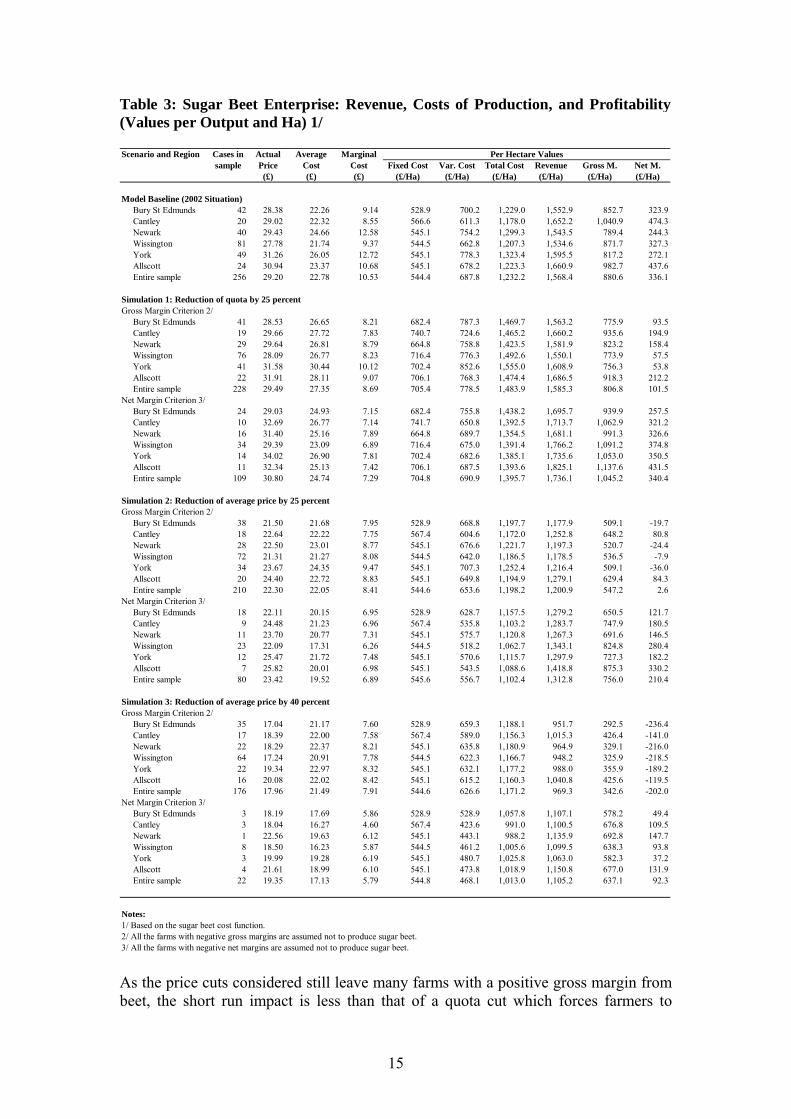
Table 3: Sugar Beet Enterprise: Revenue, Costs of Production, and Profitability(Values per Output and Ha) 1/ Scenario and Region Cases in Actual Average Marginal Per Hectare Values

sample Price Cost Cost Fixed Cost Var. Cost Total Cost Revenue Gross M. Net M.(£) (£) (£) (£/Ha) (£/Ha) (£/Ha) (£/Ha) (£/Ha) (£/Ha)

Model Baseline (2002 Situation) Bury St Edmunds 42 28.38 22.26 9.14 528.9 700.2 1,229.0 1,552.9 852.7 323.9 Cantley 20 29.02 22.32 8.55 566.6 611.3 1,178.0 1,652.2 1,040.9 474.3 Newark 40 29.43 24.66 12.58 545.1 754.2 1,299.3 1,543.5 789.4 244.3 Wissington 81 27.78 21.74 9.37 544.5 662.8 1,207.3 1,534.6 871.7 327.3 York 49 31.26 26.05 12.72 545.1 778.3 1,323.4 1,595.5 817.2 272.1 Allscott 24 30.94 23.37 10.68 545.1 678.2 1,223.3 1,660.9 982.7 437.6 Entire sample 256 29.20 22.78 10.53 544.4 687.8 1,232.2 1,568.4 880.6 336.1

Simulation 1: Reduction of quota by 25 percentGross Margin Criterion 2/ Bury St Edmunds 41 28.53 26.65 8.21 682.4 787.3 1,469.7 1,563.2 775.9 93.5 Cantley 19 29.66 27.72 7.83 740.7 724.6 1,465.2 1,660.2 935.6 194.9 Newark 29 29.64 26.81 8.79 664.8 758.8 1,423.5 1,581.9 823.2 158.4 Wissington 76 28.09 26.77 8.23 716.4 776.3 1,492.6 1,550.1 773.9 57.5 York 41 31.58 30.44 10.12 702.4 852.6 1,555.0 1,608.9 756.3 53.8 Allscott 22 31.91 28.11 9.07 706.1 768.3 1,474.4 1,686.5 918.3 212.2 Entire sample 228 29.49 27.35 8.69 705.4 778.5 1,483.9 1,585.3 806.8 101.5Net Margin Criterion 3/ Bury St Edmunds 24 29.03 24.93 7.15 682.4 755.8 1,438.2 1,695.7 939.9 257.5 Cantley 10 32.69 26.77 7.14 741.7 650.8 1,392.5 1,713.7 1,062.9 321.2 Newark 16 31.40 25.16 7.89 664.8 689.7 1,354.5 1,681.1 991.3 326.6 Wissington 34 29.39 23.09 6.89 716.4 675.0 1,391.4 1,766.2 1,091.2 374.8 York 14 34.02 26.90 7.81 702.4 682.6 1,385.1 1,735.6 1,053.0 350.5 Allscott 11 32.34 25.13 7.42 706.1 687.5 1,393.6 1,825.1 1,137.6 431.5 Entire sample 109 30.80 24.74 7.29 704.8 690.9 1,395.7 1,736.1 1,045.2 340.4

Simulation 2: Reduction of average price by 25 percentGross Margin Criterion 2/ Bury St Edmunds 38 21.50 21.68 7.95 528.9 668.8 1,197.7 1,177.9 509.1 -19.7 Cantley 18 22.64 22.22 7.75 567.4 604.6 1,172.0 1,252.8 648.2 80.8 Newark 28 22.50 23.01 8.77 545.1 676.6 1,221.7 1,197.3 520.7 -24.4 Wissington 72 21.31 21.27 8.08 544.5 642.0 1,186.5 1,178.5 536.5 -7.9 York 34 23.67 24.35 9.47 545.1 707.3 1,252.4 1,216.4 509.1 -36.0 Allscott 20 24.40 22.72 8.83 545.1 649.8 1,194.9 1,279.1 629.4 84.3 Entire sample 210 22.30 22.05 8.41 544.6 653.6 1,198.2 1,200.9 547.2 2.6Net Margin Criterion 3/ Bury St Edmunds 18 22.11 20.15 6.95 528.9 628.7 1,157.5 1,279.2 650.5 121.7 Cantley 9 24.48 21.23 6.96 567.4 535.8 1,103.2 1,283.7 747.9 180.5 Newark 11 23.70 20.77 7.31 545.1 575.7 1,120.8 1,267.3 691.6 146.5 Wissington 23 22.09 17.31 6.26 544.5 518.2 1,062.7 1,343.1 824.8 280.4 York 12 25.47 21.72 7.48 545.1 570.6 1,115.7 1,297.9 727.3 182.2 Allscott 7 25.82 20.01 6.98 545.1 543.5 1,088.6 1,418.8 875.3 330.2 Entire sample 80 23.42 19.52 6.89 545.6 556.7 1,102.4 1,312.8 756.0 210.4

Simulation 3: Reduction of average price by 40 percentGross Margin Criterion 2/ Bury St Edmunds 35 17.04 21.17 7.60 528.9 659.3 1,188.1 951.7 292.5 -236.4 Cantley 17 18.39 22.00 7.58 567.4 589.0 1,156.3 1,015.3 426.4 -141.0 Newark 22 18.29 22.37 8.21 545.1 635.8 1,180.9 964.9 329.1 -216.0 Wissington 64 17.24 20.91 7.78 544.5 622.3 1,166.7 948.2 325.9 -218.5 York 22 19.34 22.97 8.32 545.1 632.1 1,177.2 988.0 355.9 -189.2 Allscott 16 20.08 22.02 8.42 545.1 615.2 1,160.3 1,040.8 425.6 -119.5 Entire sample 176 17.96 21.49 7.91 544.6 626.6 1,171.2 969.3 342.6 -202.0Net Margin Criterion 3/ Bury St Edmunds 3 18.19 17.69 5.86 528.9 528.9 1,057.8 1,107.1 578.2 49.4 Cantley 3 18.04 16.27 4.60 567.4 423.6 991.0 1,100.5 676.8 109.5 Newark 1 22.56 19.63 6.12 545.1 443.1 988.2 1,135.9 692.8 147.7 Wissington 8 18.50 16.23 5.87 544.5 461.2 1,005.6 1,099.5 638.3 93.8 York 3 19.99 19.28 6.19 545.1 480.7 1,025.8 1,063.0 582.3 37.2 Allscott 4 21.61 18.99 6.10 545.1 473.8 1,018.9 1,150.8 677.0 131.9 Entire sample 22 19.35 17.13 5.79 544.8 468.1 1,013.0 1,105.2 637.1 92.3

Notes:1/ Based on the sugar beet cost function.2/ All the farms with negative gross margins are assumed not to produce sugar beet.3/ All the farms with negative net margins are assumed not to produce sugar beet. As the price cuts considered still leave many farms with a positive gross margin from beet, the short run impact is less than that of a quota cut which forces farmers to

15

reduce their production by the quota amount. However, under the net margin criteria the price cuts begin to have a much more significant impact. For example, a 40 per cent reduction is estimated to reduce production by over 80 per cent. Of course, it should be noted that these estimates are based on current production costs and structures. The actual impacts will depend upon the ability of farmers to restructure their sugar beet in the face of reform. One aspect of the results that warrants further attention is the impact of quota cuts on production. It might be assumed that a 25 per cent reduction in quota will simply lead to a 25 per cent reduction in production in the short and long run. However, the model suggests that cuts in quota lead to higher unit costs of production (see average cost in table 3) and therefore farms currently growing may well cease production altogether rather than simply cut back by the 25 percent, when one observes the results according to the gross margin criterion. The net margin figures reflect two effects: on the one hand, the increase in the average cost due to the reduction in the production scale and on the other hand, the fact that under the net margin many high cost producers have ceased producing sugar beet. The results highlight differences in the regional impacts on production of the different scenarios. For example, under the 25 per cent cut and net margin criterion the fall in production is predicted to vary between around 25 per cent for Cantley (E2) to over 60 per cent for Wissington (E4). b. Results for the Farm Cropping Enterprises Tables 4 and 5 present the results for the cropping part of the farm. The criterion used in Tables 4 and 5 to decide whether a crop is planted was whether the gross margin was positive. This is undertaken because the model is based on the assumption that fixed costs are fixed and that the farm determines the allocation between crops on the basis of gross margin. At an aggregate level, all the crops increase as a response to the reduction in the sugar beet quota and the reduction in the average price for sugar beet. With the exception of winter barley, the findings do not differ significantly between scenarios. All the scenarios indicate an increase in the area destined to winter wheat, oilseed rape and potatoes, which indicate that these crops are probably going to replace, at least partially, sugar beet in the rotation. Market conditions may, however, mitigate against a significant increase in potato area. Again though it must be emphasised that these results are based upon the relative performance of the specific crops in 2002 and therefore the apparent substitution will be sensitive to changes in the relative prices.

16

Table 4: Percentage Changes in Crop Production with Respect to 2002 Situation Scenario and Region Crops

Sugar Winter Spring Spring Winter Beans Peas Oilseed PotatoesBeet Wheat Wheat Barley Barley Rape

Simulation 1: Reduction of quota by 25 percent 1/ Bury St Edmunds -25.0 5.3 11.9 0.3 2.9 12.8 7.5 6.7 6.1 Cantley -24.0 2.7 -1.5 10.7 11.1 -3.0 -0.6 0.5 4.1 Newark -27.0 1.7 0.0 27.2 7.8 -16.2 -3.7 8.6 2.0 Wissington -25.0 3.3 3.4 -1.7 25.1 1.8 7.3 3.5 1.3 York -27.9 8.6 0.0 33.5 -3.6 11.0 -24.6 13.3 10.1 Allscott -25.6 5.1 0.0 2.6 0.7 13.9 53.5 0.5 1.1 Total -25.5 4.2 6.8 6.1 10.4 4.5 3.3 5.7 2.4

Simulation 2: Reduction of average price by 25 percent Bury St Edmunds -6.24 1.54 5.65 -1.91 -0.58 5.78 3.54 0.71 2.91 Cantley -2.89 0.30 -0.19 1.38 1.40 -0.77 -0.08 -0.01 0.53 Newark -31.30 2.29 0.00 29.55 7.99 -10.90 -2.82 8.48 1.96 Wissington -15.46 1.77 2.75 -3.46 18.35 1.34 4.17 2.83 -0.34 York -40.19 11.00 0.00 22.77 1.82 8.07 -2.99 9.04 6.85 Allscott -27.88 5.59 0.00 2.83 0.78 15.32 58.84 0.53 1.23 Total -17.73 3.08 3.84 2.93 6.85 3.21 5.36 3.82 0.59

Simulation 3: Reduction of average price by 40 percent Bury St Edmunds -9.82 2.23 6.29 -1.30 0.42 6.44 3.94 2.12 3.23 Cantley -8.07 0.84 -0.53 3.87 3.91 -2.15 -0.23 -0.03 1.47 Newark -38.75 3.17 0.00 33.65 8.84 -4.19 -1.83 9.09 2.10 Wissington -21.98 2.90 3.14 -1.90 22.70 1.66 6.35 3.22 0.95 York -49.05 13.09 0.00 25.72 2.54 9.48 -1.35 10.21 8.09 Allscott -43.91 9.36 0.00 4.74 1.30 25.68 98.59 0.90 2.06 Total -24.64 4.35 4.29 4.80 8.94 5.07 9.60 4.51 1.71

Note:1/ The simulated decrease in the production of sugar beet is as close as it is possible to reach the goal of an average decrease in the sugar beet quota by 25 percent. The results from table 5 are less clear due to the number of factors affecting the results, such as the change in the portfolio of crops and therefore the change in the total cost (sugar beet is a more expensive crop to grow than the others) and total revenue or the change in the cost of producing sugar beet. The reduction in the quota shows a reduction in the profitability for all the regions. Although this final result is common for all the regions, the reasons behind the result differ slightly among them. For instance, the variable costs of some of the regions (Cantley, Newark, and Allscott) increase with respect to the baseline. All the regions and under all the scenarios show a decrease in revenues. This is explained by the fact that sugar beet is a well remunerated crop relative to other crops. The reduction quota forces substitution of a well paid crop by other less profitable crops. In the case of the reduction in the support price the result is a combination of a lower price together with planting crops with lower prices than the baseline prices for sugar beet. With respect to the results related to the reduction in support price, since all the regions show lower revenues than the baseline revenues, the economic result (i.e., gross margins) will depend on the savings in variable costs made in each region, and which are associated to the new portfolio of crops.

17

Table 5: Farm Cropping Enterprises: Revenue, Costs of Production, andProfitability (Values per Output and Ha) 1/ 2/ Scenario and Region Actual Ratio Total Cost Marginal Per Hectare Values

Price 3/ to Total Revenue Cost 3/ Var. Cost Revenue Gross M.(£) (Ratio) (£) (£/Ha) (£/Ha) (£/Ha)

Model Baseline (2002 Situation) Bury St Edmunds 28.38 1.16 7.50 345.9 793.9 447.9 Cantley 29.02 1.02 6.72 352.2 917.1 565.0 Newark 29.43 1.54 21.16 596.1 773.4 177.2 Wissington 27.78 1.11 9.50 440.7 987.0 546.4 York 31.26 1.55 20.27 724.3 848.6 124.4 Allscott 30.94 1.80 25.97 838.3 987.4 149.2 Entire sample 29.20 1.33 14.38 534.1 890.0 356.0

Simulation 1: Reduction of quota by 25 percent Bury St Edmunds 28.32 1.24 7.16 340.6 765.8 425.2 Cantley 29.07 1.18 7.95 390.5 857.5 467.0 Newark 29.41 1.61 17.01 601.8 754.3 152.5 Wissington 27.81 1.15 7.74 428.5 974.0 545.5 York 31.16 1.51 15.64 714.8 821.3 106.5 Allscott 31.02 2.29 20.59 847.3 939.6 92.3 Entire sample 29.20 1.42 11.56 534.2 864.6 330.4

Simulation 2: Reduction of average price by 25 percent Bury St Edmunds 21.24 1.17 6.48 341.6 791.9 450.3 Cantley 21.81 1.07 5.98 358.0 888.9 530.9 Newark 22.06 1.60 17.03 585.9 748.2 162.3 Wissington 20.86 1.12 7.66 429.7 986.1 556.5 York 23.37 1.68 15.77 750.3 819.4 69.1 Allscott 23.26 2.30 20.65 850.2 936.7 86.5 Entire sample 21.90 1.42 11.22 574.7 873.5 298.8

Simulation 3: Reduction of average price by 40 percent Bury St Edmunds 16.99 1.18 6.60 341.5 786.8 445.3 Cantley 17.44 1.10 6.39 366.3 881.4 515.2 Newark 17.65 1.57 17.44 555.3 735.9 180.5 Wissington 16.69 1.14 7.63 428.4 977.7 549.3 York 18.70 1.73 16.03 750.6 797.2 46.6 Allscott 18.61 2.34 19.65 847.0 922.0 75.0 Entire sample 17.52 1.44 11.27 569.8 861.8 292.1

Notes:1/ Based on the variable cost function for all the crops in the farm.2/ Unless explicitely mentioned the figures correspond for all the crops.3/ Sugar beet. Finally, based on framework presented in figure 1, table 6 estimates the inefficiency (deadweight loss) and the rent for the current regime (“entire regime”) assuming two different free market prices (£17.50 and £16 per tonne, equivalent to a 40 and 45 percent reduction in the average support price of £29.10, respectively). In addition, the table presents an estimate of the inefficiency when the support price produces a total level of output equal to the quota (“only quota”). Under this situation it is assumed that the quota is produced by the most efficient growers.

18

Table 6: Estimate of the Inefficiencies of Supporting Sugar Beet Prices (£m) Free market sugar beet price 1/

£17.5/tonne £16.0/tonne

Total Support (Entire regime) 102.08 128.48 Rent 59.55 73.73 Deadweight loss (inefficiency) 42.53 54.75

Total Support (Only quota 2/) 21.12 47.52 Rent 12.32 37.49 Deadweight loss (inefficiency) 8.8 10.03

1/ Free market price estimated at 40 and 45 per cent lower than current average support price. Figures computed using the net margin criteria.2/ The price at which efficient UK growers will produce sufficient quantity to fulfil the national quota was estimated at £19.90 per tonne. Conclusions The analysis has considered the impacts on production and profitability three reform scenarios: a 25 per cent cut in UK quota, a 25 per cent cut in price, a 40 per cent cut in price. Using panel data from the Farm Business Survey for England, the paper estimates two cost functions: one for the sugar enterprise and another for the cropping part of the farm (i.e., excludes any livestock enterprise) and use them to analyse the impacts of the reform measures. It is clear from the analysis that the largest gains in terms of economic efficiency (productions of sugar beet at the least cost) would be achieved by a reduction in price instead of a reduction in quota. From both price cuts the one by 40 per cent is the one that produces the greater aggregate reduction in cost. However, the models suggest that this would also lead to the greatest reduction in production, some 84 per cent when the net margin criterion is considered as the relevant to exit the production of sugar beet. It is important to emphasise that the reduction in average cost obtained from this analysis is not due to a change in the ways farmers operate but basically due to the fact that those farmers with the highest cost producing sugar beet are going to quit its production. Estimation results indicate that quota reduction is accompanied with an increase in the average cost of production and therefore it might be consider just a measure to reduce budget outlays instead of a way to increase economic efficiency.

19

References Ali, Farman and Parikh, Ashok (1992). Relationships among Labor, Bullock, and Tractor Inputs in Pakistan Agriculture. American Journal of Agricultural Economics, 74(2):371-77. Alvarez, Antonio and Arias, Carlos (2003). Diseconomies of Size with Fixed Managerial Ability. American Journal of Agricultural Economics, 85(1):135-42 Amadi, Juliana, Piesse, Jenifer and Thirtle, Colin (2004). Crop Level Productivity in the Eastern Counties of Eangland, 1970-97. Journal of Agricultural Economics, 55(2):367-83. Berndt, Ernst R. and Wood, David O. (1975). Technology, Prices and the Derived Demand for Energy. The Review of Economics and Statistics, 57(3): 259-68. Binswanger, Hans P. (1974). A Cost Function Approach to the Measurement of Elasticities of Factor Demand and Elasticities of Substitution. American Journal of Agricultural Economics. 56(2): 377-86. Caves, Douglas W., Christensen, Laurits R. and Tretheway, Michael W. (1981). Flexible Cost Funtions for Multiproduct Firms. Review of Economic and Statistics, 62(1): 477-81. Chambers, Robert G. (1988). Applied production analysis: A dual approach. New York: Cambridge University Press. Christensen, Laurits R. and Jorgenson, Dale W. (1970). U.S. Real Product and Real Factor Input, 1929-1967. Review of Income and Wealth, 16(1): 19-50. Commission of the European Communities (CEC) (2004). Communication from the Commission to the Council and the European Parliament: Accomplishing a Sustainable Agricultural Model for Europe through the Reformed CAP – Sugar Sector Reform. COM(2004) 499 final. Available online: http://europa.eu.int/eur-lex/en/com/cnc/2004/com2004_0499en01.pdf Fuss, Melvyn and McFadden, Daniel L. (eds.) (1978). Production Economics: A Dual Approach to Theory and Applications. Amsterdam: North Holland. Guyomard, H, Delache, X., Irz, X. and Mahe, L.P. (1996) A Micro-econometric Analysis of Milk Quota Transfer: Application to French Producers. Journal of Agricultural Economics, 47(2): 206-23. Hsiao, Cheng (1993). Analysis of Panel Data. Econometric Society Monographs No. 11, New York: Cambridge University Press. Mundlak, Yair (1978). On the Pooling of Time Series and Cross Section Data. Econometrica, 46(1): 69-85.

20

Nerlove, Marc L. (1958). The Dynamics of Supply: Estimation of Farmers' Response to Price. Baltimore: The Johns Hopkins Press. Renwick A. (1997). Economics of the UK Sugar Beet Industry, MAFF Special Studies in Agricultural Economics Report Number 35. Department of Land Economy, University of Cambridge. Renwick A., Revoredo Giha, C., and Reader, M. (2005), UK Sugar Beet Farm Productivity under Different Reform Scenarios: A Farm Level Analysis. Environmental Economy and Policy Research Discussion Paper 04.2005, Department of Land Economy, University of Cambridge. Available online: http://www.landecon.cam.ac.uk/RePEc/lnd/042005%20Revoredo.pdf Rural Business Unit (RBU), University of Cambridge (2004) Economic, Social and Environmental Implications of EU Sugar Regime, DEFRA Economic Report. Available online: http://statistics.DEFRA.gov.uk/esg/reports/sugar/default.asp Walters, A.A. Expectations and the Regression Fallacy in Estimating Cost Functions. Review of Economics and Statistics, 42(2): 210-15.

21

Appendix a. Estimation Results Table A.1: Variable Cost Function: Regression Results for the Sugar Beet Enterprise 1/ 2/

Dependent Variable: Log(Variable Cost)Log-Likelihood - factor demands block : 7,845.19

Variable Coefficient t -stat.

Box-Cox λ 0.215040 9.843W1 0.149890 24.368W2 0.092475 10.623W3 0.215730 23.963W4 -0.003700 -2.085W5 0.545610 33.928

W1*W1 0.061282 3.481W1*W2 0.016588 1.650W1*W3 -0.065658 -6.800W1*W4 -0.010209 -1.292W1*W5 -0.002003 -0.080W2*W1 0.016588 1.650W2*W2 0.081911 5.580W2*W3 0.054337 5.112W2*W4 0.000277 0.072W2*W5 -0.153110 -6.836W3*W1 -0.065658 -6.800W3*W2 0.054337 5.112W3*W3 0.141610 9.503W3*W4 -0.011110 -1.308W3*W5 -0.119180 -5.231W4*W1 -0.010209 -1.292W4*W2 0.000277 0.072W4*W3 -0.011110 -1.308W4*W4 0.044484 1.130W4*W5 -0.023443 -0.822W5*W1 -0.002003 -0.080W5*W2 -0.153110 -6.836W5*W3 -0.119180 -5.231W5*W4 -0.023443 -0.822W5*W5 0.297740 5.485W1*Q 0.001346 4.094W1*Q 0.005193 10.988W1*Q 0.001693 3.468W1*Q 0.000390 4.149W1*Q -0.008622 -9.891

Q 0.152690 5.184Q*Q -0.002190 -1.497

Notes:1/ Variables are in logs or transformed by the Box-Cox transformation.2/ Standard deviation was computed using the heteroskedasticity-consistent covariance matrix.

22

Table A.2: Variable Cost Function: Regression Results for the Cropping Area of the Farm 1/ 2/

Dependent Variable: Log(Variable Cost)Log-Likelihood - factor demands block : 7,845.19Log-Likelihood - only output block: 1,138.76

Variable Coefficient t -stat. Variable Coefficient t -stat.

Box-Cox λ 0.338000 Grid Search W5*Q1 0.002728 8.440W1 0.220338 44.584 W5*Q2 -0.004042 -13.180W2 0.192743 33.990 W5*Q3 0.003755 7.390W3 0.343697 48.870 W5*Q4 0.000527 1.617W4 0.047666 2.200 W5*Q5 -0.002556 -8.975W5 0.195556 23.009 W5*Q6 0.000622 1.376

W1*W1 -0.017090 -0.741 W5*Q7 0.001616 3.905W1*W2 0.004160 0.259 W5*Q8 -0.000167 -0.389W1*W3 0.028968 1.447 W5*Q9 -0.002482 -15.712W1*W4 -0.033366 -1.125 Q1 0.009944 15.765W1*W5 0.017328 0.629 Q2 0.005453 14.344W2*W1 0.004160 0.259 Q3 0.001770 5.493W2*W2 0.166006 8.568 Q4 0.001039 4.768W2*W3 -0.072119 -4.539 Q5 0.002810 9.331W2*W4 -0.029935 -1.131 Q6 0.001472 5.347W2*W5 -0.068111 -2.646 Q7 0.001405 4.146W3*W1 0.028968 1.447 Q8 0.001670 6.452W3*W2 -0.072119 -4.539 Q9 0.008434 20.749W3*W3 0.091094 3.613 Q1*Q1 0.000086 6.379W3*W4 0.059153 1.767 Q1*Q2 0.000063 10.876W3*W5 -0.107096 -3.530 Q1*Q3 0.000018 3.402W4*W1 -0.033366 -0.024 Q1*Q4 0.000020 4.796W4*W2 -0.029935 -2.949 Q1*Q5 0.000007 1.153W4*W3 0.059153 2.792 Q1*Q6 0.000030 4.844W4*W4 -0.188132 -3.395 Q1*Q7 0.000017 2.203W4*W5 0.192281 3.611 Q1*Q8 -0.000028 -4.643W5*W1 0.017328 0.629 Q1*Q9 0.000025 3.559W5*W2 -0.068111 -2.646 Q2*Q2 0.000368 15.631W5*W3 -0.107096 -3.530 Q2*Q3 0.000007 0.613W5*W4 0.192281 2.373 Q2*Q4 -0.000035 -2.812W5*W5 -0.034402 -0.460 Q2*Q5 -0.000010 -0.904W1*Q1 -0.000139 -0.768 Q2*Q6 0.000022 2.486W1*Q2 -0.000815 -4.746 Q2*Q7 0.000035 3.456W1*Q3 -0.000458 -1.612 Q2*Q8 0.000074 8.708W1*Q4 -0.000053 -0.288 Q2*Q9 0.000031 2.605W1*Q5 0.000432 2.710 Q3*Q3 0.000223 4.433W1*Q6 -0.000166 -0.655 Q3*Q4 -0.000138 -3.417W1*Q7 0.000885 3.824 Q3*Q5 0.000092 2.577W1*Q8 -0.001349 -5.626 Q3*Q6 0.000173 3.068W1*Q9 0.001661 18.796 Q3*Q7 0.000127 1.376W2*Q1 -0.000344 -1.586 Q3*Q8 -0.000131 -1.738W2*Q2 0.001880 9.140 Q3*Q9 -0.000002 -0.061W2*Q3 -0.001484 -4.355 Q4*Q4 0.000189 5.068W2*Q4 0.001003 4.582 Q4*Q5 -0.000006 -0.346W2*Q5 0.001967 10.305 Q4*Q6 -0.000014 -0.335W2*Q6 -0.000144 -0.475 Q4*Q7 -0.000138 -2.980W2*Q7 -0.001864 -6.716 Q4*Q8 -0.000154 -4.257W2*Q8 0.000686 2.387 Q4*Q9 0.000075 3.515W2*Q9 -0.001699 -16.025 Q5*Q5 0.000326 10.176W3*Q1 -0.001968 -7.298 Q5*Q6 -0.000067 -2.719W3*Q2 0.003132 12.239 Q5*Q7 -0.000041 -1.306W3*Q3 -0.000694 -1.637 Q5*Q8 -0.000066 -2.829W3*Q4 -0.000767 -2.819 Q5*Q9 -0.000086 -3.601W3*Q5 0.000445 1.872 Q6*Q6 0.000021 0.308W3*Q6 0.000103 0.272 Q6*Q7 0.000084 1.126W3*Q7 0.000580 1.678 Q6*Q8 -0.000041 -0.773W3*Q8 0.000084 0.235 Q6*Q9 -0.000167 -4.027W3*Q9 -0.000914 -6.932 Q7*Q7 0.000052 1.434W4*Q1 -0.000258 -1.381 Q7*Q8 -0.000086 -1.061W4*Q2 0.000019 0.107 Q7*Q9 -0.000057 -1.758W4*Q3 -0.001415 -4.815 Q8*Q8 0.000685 12.454W4*Q4 -0.000566 -3.008 Q8*Q9 -0.000107 -2.695W4*Q5 0.000546 3.318 Q9*Q9 0.000243 6.440W4*Q6 -0.000293 -1.124W4*Q7 -0.001040 -4.353W4*Q8 -0.000104 -0.420W4*Q9 0.003111 34.113

Notes:1/ Variables are in logs or transformed by the Box-Cox transformation.2/ Standard deviation was computed using the heteroskedasticity-consistent covariance matrix.

23

b. Procedure followed to constrain the total agricultural area to be unchanged

Since it was not possible to constraint the parameters of the cost function to produce a change in the area of the other crops equal to the reduction in the area under sugar beet, we rescaled the results obtained from the model so the reduction in the area dedicated to sugar beet was absorbed according to the directions indicated to the model. We performed this change in scale by considering the information about the cropping area by region and by simulation scenario. The starting point was the condition that the decrease in the sugar beet area in the region j ( ) with respect to the base case had to be distributed by considering the

changes in the other crops. Mathematically this is equal to (A.1):

BeetjA∆

( ) ∑ ∆=∆−

=

9

2i

ij

Beetj AA1.A

The scaling weight for the region j is then equal to:

( )( )∑ −

∆−=γ

=

9

2i

i,0j

i,Uj

Beetj

jAA

A2.A

Where i is the (unadjusted) area in region j for crop i predicted by the model after

simulating the change in policy, and is the area in the baseline case for crop i.

Therefore, for region j it has to hold the following condition:

,UjA

i,0jA

( ) ∑ ∑ ∆⋅γ=∆

= =

9

2i

9

2i

i,Ujj

i,Fj AA3.A

Where is the change in the area of the crop i after we have scaled

the unadjusted results. In addition, it should be noted that

i,0j

i,Fj

i,Fj AAA −=∆

)A(A9

2i

Beetjj

i,Fj∑ ∆−⋅γ=∆

=

.

Operating (3) we can arrive to the following condition:

( ) ( ) ∑⋅γ−+∑ ∑⋅γ=== =

9

2i

i,0jj

9

2i

9

2i

i,Ujj

i,Fj A1AA4.A

Our goal is to find a set of that satisfies (A.4). There are several ways to do this;

however, an appealing solution is one that conserves the sign in the change in area predicted by the model. Hence, we choose the following solution to (A.4) that says that the final area is a linear combination of the baseline solution and the unadjusted solution. This is:

i,FjA

( ) ( ) i,0

jji,U

jji,F

j A1AA5.A ⋅γ−+⋅γ=

24

It should be noted that (A.5) is also satisfied for the output, assuming that there are no changes in yields. This is easy to see after multiplying (A.5) by (crop i yield in

region j).

ijy

( ) ( ) ( ) i,0

jji,U

jjij

i,0jj

ij

i,Ujj

ij

i,Fj

i,Fj Q1QyA1yAyAQ6.A ⋅γ−+⋅γ=⋅⋅γ−+⋅⋅γ=⋅=

Finally, with respect to the change in area, dividing (A.7) by the baseline area we get:

( ) ( )ji,0j

i,Uj

ji,0j

i,Fj 1

A

A

A

A7.A γ−+⋅γ=

Which can be simplified as:

( )

( ) i,0j

i,Uj

ji,0j

i,Fj

ji,0j

i,Uj

ji,0j

i,Fj

A

A

A

A8.A

1A

A1

A

A1

∆⋅γ=

∆

γ−+⎟⎟⎟

⎠

⎞

⎜⎜⎜

⎝

⎛ ∆+⋅γ=

⎟⎟⎟

⎠

⎞

⎜⎜⎜

⎝

⎛ ∆+

25