Embed Size (px)
Citation preview
1
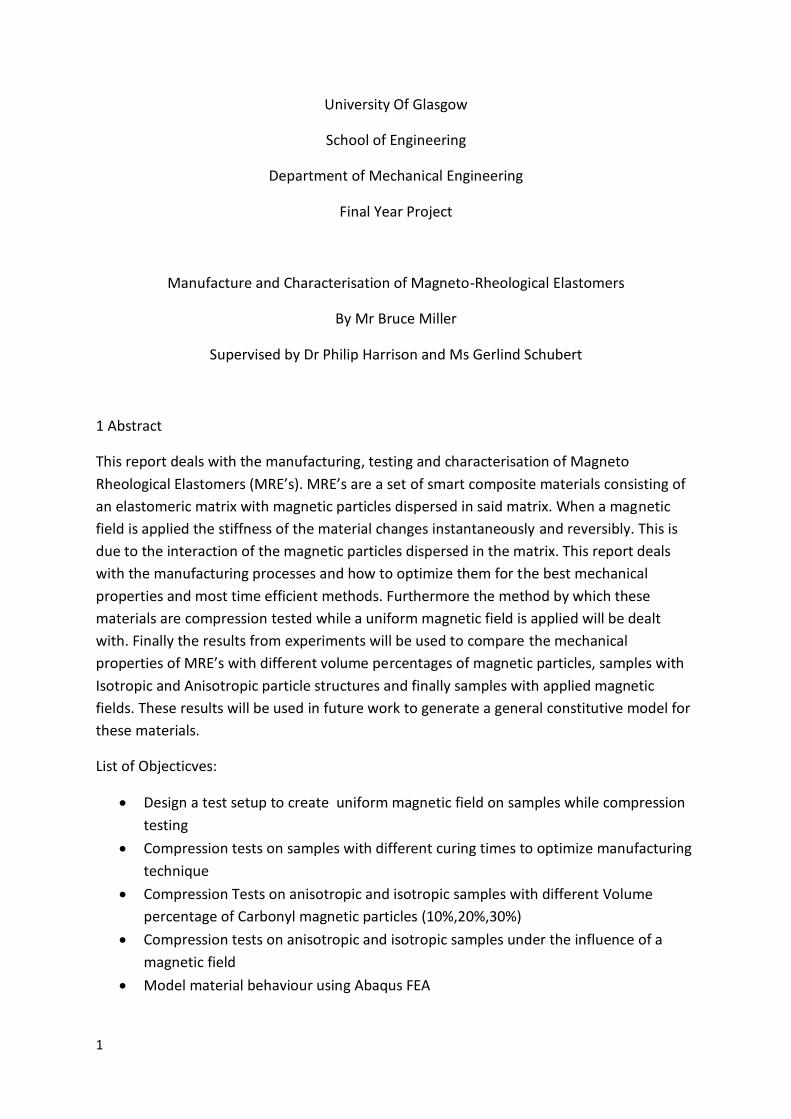
University Of Glasgow
School of Engineering
Department of Mechanical Engineering
Final Year Project
Manufacture and Characterisation of Magneto-Rheological Elastomers
By Mr Bruce Miller
Supervised by Dr Philip Harrison and Ms Gerlind Schubert
1 Abstract
This report deals with the manufacturing, testing and characterisation of Magneto
Rheological Elastomers (MRE’s). MRE’s are a set of smart composite materials consisting of
an elastomeric matrix with magnetic particles dispersed in said matrix. When a magnetic
field is applied the stiffness of the material changes instantaneously and reversibly. This is
due to the interaction of the magnetic particles dispersed in the matrix. This report deals
with the manufacturing processes and how to optimize them for the best mechanical
properties and most time efficient methods. Furthermore the method by which these
materials are compression tested while a uniform magnetic field is applied will be dealt
with. Finally the results from experiments will be used to compare the mechanical
properties of MRE’s with different volume percentages of magnetic particles, samples with
Isotropic and Anisotropic particle structures and finally samples with applied magnetic
fields. These results will be used in future work to generate a general constitutive model for
these materials.
List of Objecticves:
Design a test setup to create uniform magnetic field on samples while compression
testing
Compression tests on samples with different curing times to optimize manufacturing
technique
Compression Tests on anisotropic and isotropic samples with different Volume
percentage of Carbonyl magnetic particles (10%,20%,30%)
Compression tests on anisotropic and isotropic samples under the influence of a
magnetic field
Model material behaviour using Abaqus FEA
2
Table of Contents
List of Figures ........................................................................................................................................ 3
List of Equations.................................................................................................................................... 3
List of Tables ......................................................................................................................................... 4
Glossary of Nomenclature .................................................................................................................... 4
Acknoledgements ................................................................................................................................. 5
Introduction .......................................................................................................................................... 5
Background Information ....................................................................................................................... 5
Manufacturing Process ......................................................................................................................... 6
Test Method ......................................................................................................................................... 9
Test Setup ........................................................................................................................................... 10
Test Results ......................................................................................................................................... 13
Pure Rubber, 10%, 20%, 30% Isotropic samples cured for 24 Hours at 25oC .................................. 14
Compression of Pure Rubber with different curing conditions ....................................................... 17
Compression of 10% volume Isotropic samples with different curing conditions .......................... 18
Compression of 10%, 20% and 30% Anisotropic samples ............................................................... 19
Compression of 10%, 20% and 30%, Anisotropic and Isotropic Samples with applied magnetic
fields ............................................................................................................................................... 22
10% Isotropic Samples ................................................................................................................ 23
20% Isotropic Samples ................................................................................................................ 24
30% Isotropic Samples ................................................................................................................ 25
10% Anisotrpic Samples .............................................................................................................. 26
20% Anisotropic Samples ............................................................................................................ 27
30% Anisotropic Samples ............................................................................................................ 28
Modelling of MREs .............................................................................................................................. 29
Modelling of 10% Isotropic Samples ........................................................................................... 30
Modelling of 20% Isotropic Samples ........................................................................................... 34
Modelling of 30% Isotropic Samples ........................................................................................... 38
Modelling of Pure Rubber ........................................................................................................... 42
Conclusions ......................................................................................................................................... 43
Bibliography ........................................................................................................................................ 44
Appendix A : Calculation for Solenoids ............................................................................................... 45
Appendix B: Faulty test setup results .................................................................................................. 47
3
List of Figures
Figure 1 Picture of Heating Plates ......................................................................................................... 8
Figure 2 Picture of Electromagnet with mould in between poles ......................................................... 9
Figure 3 Picture of Electromagnet ........................................................................................................ 9
Figure 4 Original Magnetic Setup ........................................................................................................ 11
Figure 5 Revised Magnetic Setup ........................................................................................................ 11
Figure 6 Rendered Drawing of Test Setup........................................................................................... 12
Figure 7 Picture of Test Setup ............................................................................................................. 12
Figure 8 ............................................................................................................................................... 14
Figure 9 Microscopic Picture of 10% Isotropic Sample ....................................................................... 15
Figure 10 Microscopic Picture of 20% Isotropic Sample ..................................................................... 15
Figure 11 Graph of all Isotropic Sample Configurations ...................................................................... 16
Figure 12 Graph of Pure Rubber with different Curing Conditions ..................................................... 17
Figure 13 Graph of 10%v CIP samples with different curing conditions.............................................. 18
Figure 14 Microscopic Picture of 10% Anisotropic Sample ................................................................. 19
Figure 15 Buckling Samples ................................................................................................................. 20
Figure 16 Graph of all volume percentages of CIP for Anisotropic and Isotropic structures ............... 21
Figure 17 Graph of 10% Isotropic CIP Samples with different applied magnetic fields ....................... 23
Figure 18 Graph of 20% Isotropic CIP Samples with different applied magnetic fields ....................... 24
Figure 19 Graph of 30% Isotropic Samples with different applied magnetic fields ............................. 25
Figure 20 Graph of 30% Anisotropic Samples with different applied magnetic fields ........................ 26
Figure 21Graph of 20% Anisotropic samples with different applied magnetic fields .......................... 27
Figure 22 Graph of 30% Anisotropic samples with different applied magnetic fields ......................... 28
Figure 23 10% Isotropic Samples with 400mT applied magnetic field ................................................ 30
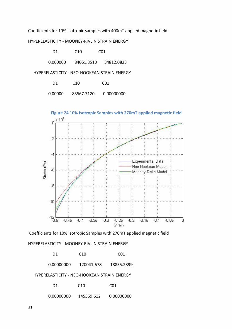
Figure 24 10% Isotropic Samples with 270mT applied magnetic field ................................................ 31
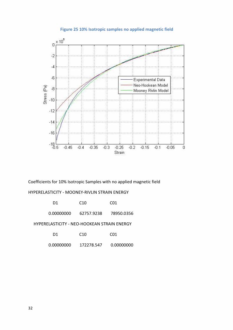
Figure 25 10% Isotropic samples no applied magnetic field ............................................................... 32
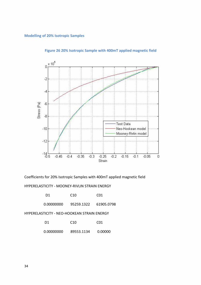
Figure 26 20% Isotropic Sample with 400mT applied magnetic field .................................................. 34
Figure 27 20% Isotropic Samples with 270mT applied magnetic field ................................................ 35
Figure 28 20% Isotropic Samples with no applied magnetic field ....................................................... 36
Figure 29 30% Isotropic Samples with 400mT applied magnetic field ................................................ 38
Figure 30 30% Isotropic Samples with 270mT applied magnetic field ................................................ 39
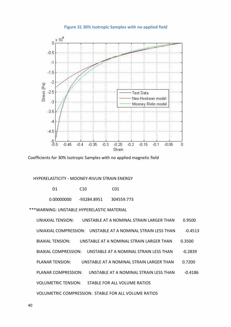
Figure 31 30% Isotropic Samples with no applied field ....................................................................... 40
Figure 32 Pure Rubber Modelling Curves............................................................................................ 42
List of Equations
Equation 1 Equation for Mass of CIP[] ................................................................................................... 8
Equation 2 Standard Ogden Model ..................................................................................................... 29
Equation 3 Standard Mooney Rivlin Model ........................................................................................ 29
Equation 4 Standard Neo Hookean Model ......................................................................................... 29
4
List of Tables
Table 1 Rubber Poperties ...................................................................................................................... 6
Table 2 CIP properties ........................................................................................................................... 7
Table 3 Calculation of Masses ............................................................................................................... 7
Table 4 Youngs Moduli for all Isotropic Sample Configurations .......................................................... 16
Table 5 Youngs Moduli of Pure Rubber with different Curing Times .................................................. 17
Table 6 Youngs Moduli of 10%v CIP samples with different curing times ........................................... 18
Table 7 Youngs Moduli for Anisotropic Samples ................................................................................. 21
Table 8 Table of Youngs Moduli for 10% Isotropic Samples ................................................................ 23
Table 9 Table of Youngs Moduli for 20% Isotropic Samples ................................................................ 24
Table 10 Table of Youngs Moduli for 30% Isotropic Samples .............................................................. 25
Table 11 Table of Youngs Moduli for 10% Anisotropic samples .......................................................... 26
Table 12 Table of Young’s Moduli for 20% Anisotropic Samples ........................................................ 27
Table 13 Table of Youngs Moduli for 30% Anisotropic samples .......................................................... 28
Table 14 Table of Coefficients for Mooney-Rivlin Model .................................................................... 33
Table 15 Table of Coefficients for Neo-Hookean Model ..................................................................... 33
Table 16 Table of Coefficients for Neo-Hookean Model ..................................................................... 37
Table 17 Table of Coefficients for Mooney-Rivlin Model .................................................................... 37
Table 18 Table of R2 values for 30% Isotropic Samples ...................................................................... 41
Table 19 Youngs Modulus for 30% Isotropic Samples for Neo-Hookean Model ................................. 41
Table 20 Youngs Modulus for 30% Isotropic Samples for Mooney-Rivlin Model ................................ 41
Table 21 Youngs Moduli for Pure Rubber for Mooney Rivlin Model ................................................... 43
Table 22 Youngs Moduli for Pure Rubber Neo-Hookean model ......................................................... 43
Glossary of Nomenclature
MR effect- Magneto-Rheological effect whereby the stiffness of material increases with an
applied magnetic field
CIP- Carbonyl Iron Powder
Mullins Effect- The instantaneous softening of rubbers when the all time maximum applied
stress is reached
FEA- Finite Element Analysis
Magnetic Flux Density- This is the amount of magnetic field passing through a surface
measured in Teslas

5
Acknoledgements
I would like to thank Dr Harrison for helping me out during this project.He has always kept me
organisedand wa always giving me new suggestions and some really good ideas to work on. I would
also like to thank Gerlind Schubert for helping with all backround information on this topic as well as
the analysis parts of the project. I would also like to thank John Davidson the materials lab
technician. He really helped with the testing and the test setup.
Introduction
Magneto Rheological Elastomers are a set of smart composites whose mechanical
properties can be reversibly and instantaneously changed when a magnetic field is applied.
These materials can be used in systems where the ability to vary the stiffness of a
component is required, such as vibration control systems and variable suspension systems
in automobiles. Currently there is no available general constitutive model for these
materials and the aim of Ms Schubert’s PhD research project is to develop a constitutive
model for these materials. The objective of this project is to undertake the preliminary
compression testing of these materials to determine their stress strain behaviour.
Furthermore the manufacturing process and testing procedures will be developed and
refined throughout. The objective is to test all the relevant specimens and all configurations
possible in order to assist with the development of the constitutive model.
Background Information1
Magneto Rheological Elastomers were first studied in 1995 by Toyota Central Research and
Development Laboratories. They tested silicone gels with the magnetic particles aligned
through dynamic shear experiments with small deformations. They noted the change in
moduli due to the effects of the applied external magnetic field. Further research was
carried out by Jolly and Carlsen in 1996 at the Thomas Lord Research Centre where they also
tested silicon gels under small deformation shear with and without magnetic field and noted
the change in storage modulus due to the applied magnetic field. The first applications for
this kind of material were brought forth by the Ford Motor Company. They suggested and
implemented the material as a suspension bushing thats stiffness could be altered to
change ride comfort or handling quality of their motor cars. Kallio2 carried out many
experiments in 2003 in order to discover which materials were best to create an MR effect.
Kallio conducted mainly small strain experiments and found that the best materials are
Silicone Rubber Matrix with CIP magnetic particles. Farshad3 in 2003 conducted
compression testing up to 30% strain, using anistropic samples and isotropic samples for
testing.
1 All Backround information has been researched through Ms Gerlind Schuberts 1st Year Literature Revue 2 M. Kallio Preliminary tests on an MRE device 3 M. Farshad Magnetoactive elastomer composites
6
Furthermore testing with an applied magnetic field were conducted, although moving
magnets were used which means further steps are needed in calculations to allow for the
attractive forces of the magnets to be removed from the force measurements. Varga4 in
2005 conducted similar compression testing but chose to use a solenoid coil to apply
magnet fields to the samples. Applications for this material mainly involve vibration control
as the forced response can be controlled by changing the stiffness components in springs.
Manufacturing Process
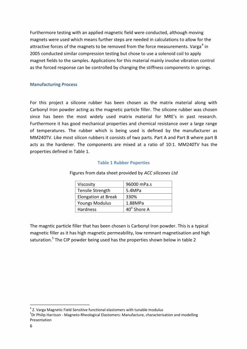
For this project a silicone rubber has been chosen as the matrix material along with
Carbonyl Iron powder acting as the magnetic particle filler. The silicone rubber was chosen
since has been the most widely used matrix material for MRE’s in past research.
Furthermore it has good mechanical properties and chemical resistance over a large range
of temperatures. The rubber which is being used is defined by the manufacturer as
MM240TV. Like most silicon rubbers it consists of two parts. Part A and Part B where part B
acts as the hardener. The components are mixed at a ratio of 10:1. MM240TV has the
properties defined in Table 1.
Table 1 Rubber Poperties
Figures from data sheet provided by ACC silicones Ltd
Viscosity 96000 mPa.s Tensile Strength 5.4MPa
Elongation at Break 330%
Youngs Modulus 1.88MPa
Hardness 40o Shore A
The magntic particle filler that has been chosen is Carbonyl Iron powder. This is a typical
magnetic filler as it has high magnetic permeability, low remnant magnetisation and high
saturation.5 The CIP powder being used has the properties shown below in table 2
4 Z. Varga Magnetic Field Sensitive functional elastomers with tunable modulus 5Dr Philip Harrison - Magneto-Rheological Elastomers: Manufacture, characterisation and modelling Presentation
7
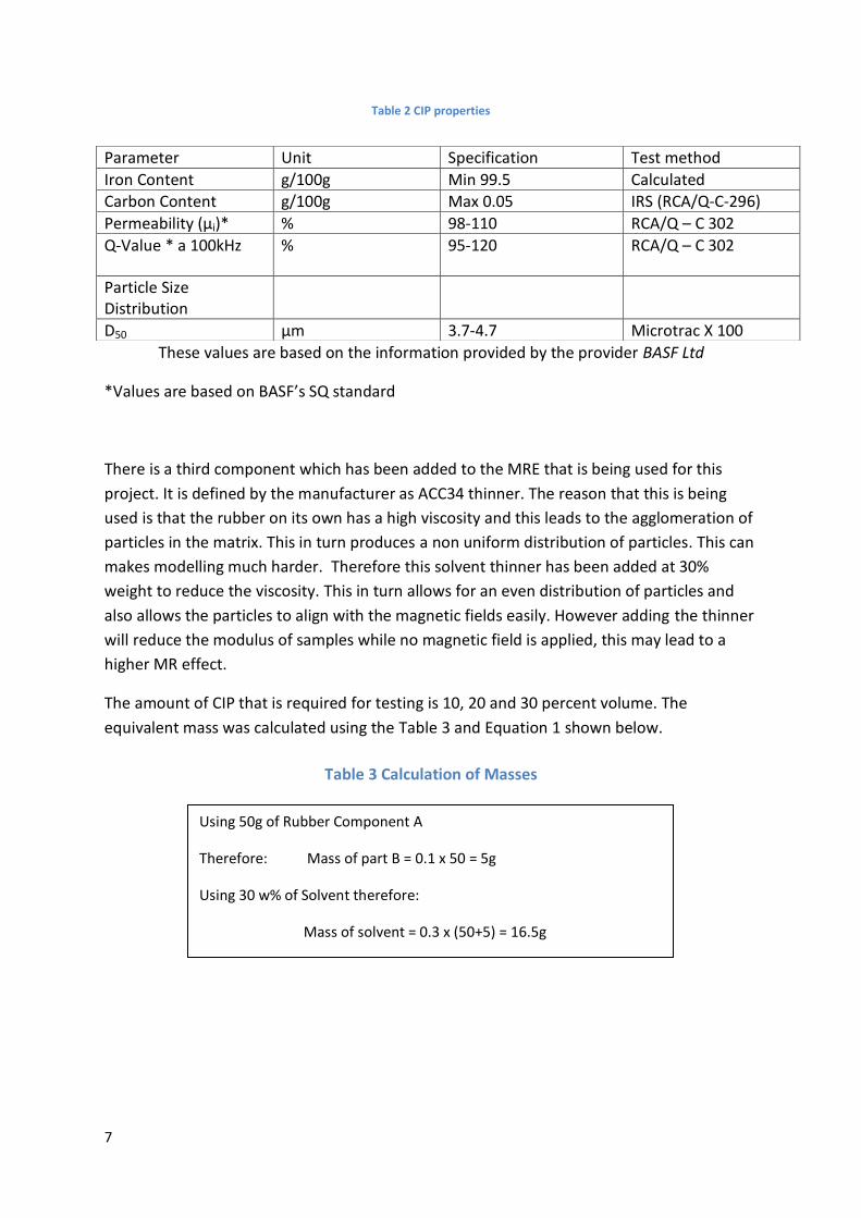
Table 2 CIP properties
These values are based on the information provided by the provider BASF Ltd
*Values are based on BASF’s SQ standard
There is a third component which has been added to the MRE that is being used for this
project. It is defined by the manufacturer as ACC34 thinner. The reason that this is being
used is that the rubber on its own has a high viscosity and this leads to the agglomeration of
particles in the matrix. This in turn produces a non uniform distribution of particles. This can
makes modelling much harder. Therefore this solvent thinner has been added at 30%
weight to reduce the viscosity. This in turn allows for an even distribution of particles and
also allows the particles to align with the magnetic fields easily. However adding the thinner
will reduce the modulus of samples while no magnetic field is applied, this may lead to a
higher MR effect.
The amount of CIP that is required for testing is 10, 20 and 30 percent volume. The
equivalent mass was calculated using the Table 3 and Equation 1 shown below.
Parameter Unit Specification Test method
Iron Content g/100g Min 99.5 Calculated Carbon Content g/100g Max 0.05 IRS (RCA/Q-C-296)
Permeability (µi)* % 98-110 RCA/Q – C 302
Q-Value * a 100kHz % 95-120 RCA/Q – C 302
Particle Size Distribution
D50 µm 3.7-4.7 Microtrac X 100
Using 50g of Rubber Component A
Therefore: Mass of part B = 0.1 x 50 = 5g
Using 30 w% of Solvent therefore:
Mass of solvent = 0.3 x (50+5) = 16.5g
Table 3 Calculation of Masses
8
Equation 1 Equation for Mass of CIP[6]
Where v = relative volume of CIP and x = required mass, 71.5g is the total mass of pure
rubber 1.06g/cm3 is density of rubber and 7.874 g/cm3 is density of CIP.
The next stage of the process was to mix the mixture thoroughly using a hand mixer for a
minimum time of three minutes. The mixture is then degassed in a vacuum chamber for ten
minutes in order to avoid air bubbles when the rubber is cured. The mixture is then poured
into moulds. These moulds are designed according to the standard sample size for test
method A of BS ISO 77427. The sample size required is 29mm ± 0.5mm diameter and
12.5mm ± 0.5mm height.
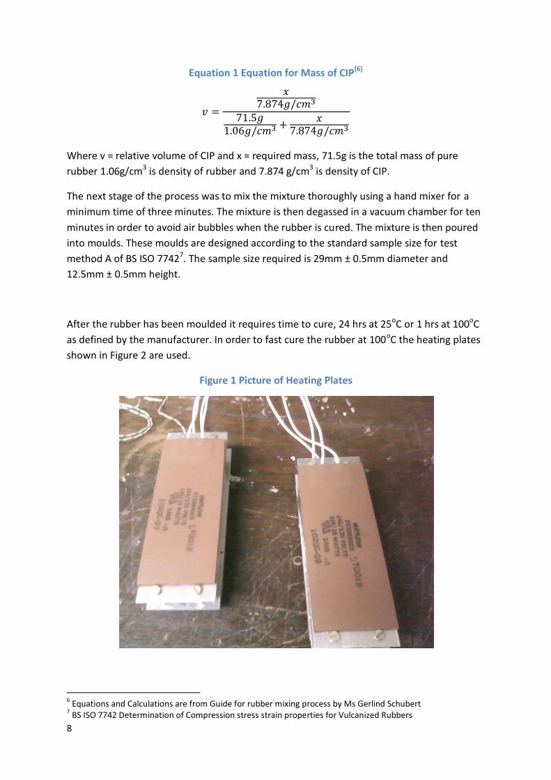
After the rubber has been moulded it requires time to cure, 24 hrs at 25oC or 1 hrs at 100oC
as defined by the manufacturer. In order to fast cure the rubber at 100oC the heating plates
shown in Figure 2 are used.
Figure 1 Picture of Heating Plates
6 Equations and Calculations are from Guide for rubber mixing process by Ms Gerlind Schubert 7 BS ISO 7742 Determination of Compression stress strain properties for Vulcanized Rubbers
9
One of the objectives for this report is to optimize the manufacturing process therefore
samples will be fast and slow cured to find the optimal curing time.
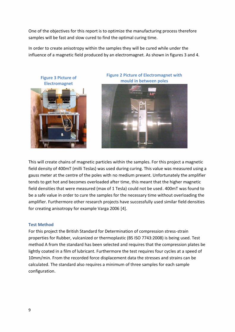
In order to create anisotropy within the samples they will be cured while under the
influence of a magnetic field produced by an electromagnet. As shown in figures 3 and 4.
This will create chains of magnetic particles within the samples. For this project a magnetic
field density of 400mT (milli Teslas) was used during curing. This value was measured using a
gauss meter at the centre of the poles with no medium present. Unfortunately the amplifier
tends to get hot and becomes overloaded after time, this meant that the higher magnetic
field densities that were measured (max of 1 Tesla) could not be used. 400mT was found to
be a safe value in order to cure the samples for the necessary time without overloading the
amplifier. Furthermore other research projects have successfully used similar field densities
for creating anisotropy for example Varga 2006 [4].
Test Method
For this project the British Standard for Determination of compression stress-strain
properties for Rubber, vulcanized or thermoplastic (BS ISO 7743:2008) is being used. Test
method A from the standard has been selected and requires that the compression plates be
lightly coated in a film of lubricant. Furthermore the test requires four cycles at a speed of
10mm/min. From the recorded force displacement data the stresses and strains can be
calculated. The standard also requires a minimum of three samples for each sample
configuration.
Figure 3 Picture of Electromagnet
Figure 2 Picture of Electromagnet with mould in between poles
10
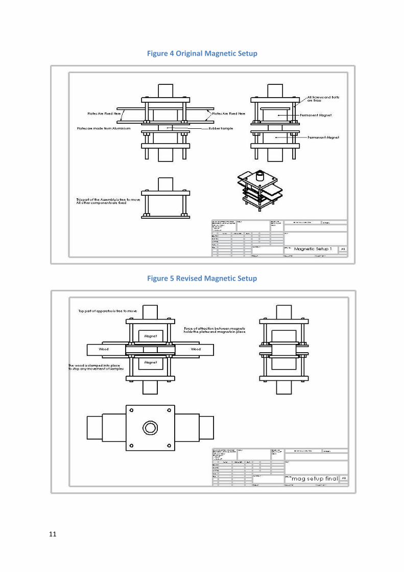
Test Setup
In order to test these materials with an applied magnetic field it is necessary to create a
device or alternative setup to allow the magnetic field to pass through the samples while
they are compressed. A paper by Varga [4] indicated that a solenoid coil was used to
implement a uniform magnetic field during testing. The aim of this project was to use quite
a high field density of 400mT, and after some calculations (see appendix A) it was decided
that the required coil would be expensive and impractical for use. Another paper by Farshad
[3] indicated that a pair of permanent magnets could be used to generate a uniform field
through the sample. The test setup used by Farshad [3] indicated that the plates be wedged
between two aluminium plates while the compression took place, thereby the magnets
would move up and down with the compression. It was decided that this method was
inaccurate due to the fact that the attractive force between the magnets would increase as
the magnets were brought closer together. This would add false readings to the load cell
and would mean that additional steps would have to be taken to interpret the results
correctly. Therefore a new test setup was designed and assembled using neodymium
permanent magnets. The technical drawing is shown in figure 4. Unfortunately when this
setup was used there were some problems with the test results (see appendix B). Therefore
the setup was reworked again the revised setup is shown in figure 5. The magnetic field
density can be altered simply by making the distance between the magnets larger or
smaller. During testing a magnetic field density of 400mT was measured between the poles
at a separation of 36mm and this decreased to around 270mT at a distance of 47mm.
From the drawings provide you will see that the magnets are held in place as the
compression plates are free to move.
11
Figure 4 Original Magnetic Setup
Figure 5 Revised Magnetic Setup
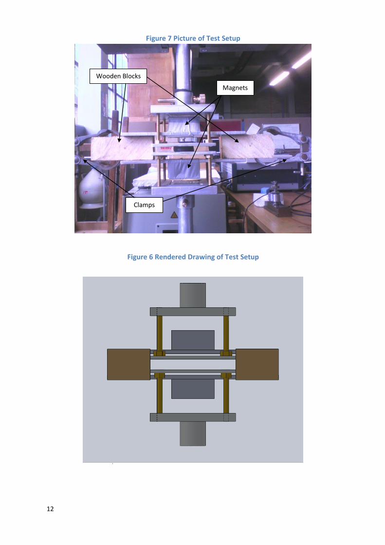
12
Figure 7 Picture of Test Setup
Figure 6 Rendered Drawing of Test Setup
Wooden Blocks
Magnets
Clamps
13
Test Results
The tests that have been completed are:
Compression of Pure rubber, 10%, 20%, 30% volume CIP cured for 24 hours at 25oC. Purely Isotropic samples.
Compression of Pure Rubber cured for 1 hour and 1.5 hours at 100 oC.
Compression of 10% volume cured for 1 hour and 1.5 hours at 100 oC. Purely Isotropic samples.
Compression of 10%, 20% and 30% Anisotropic samples cured for 1 hour at 100 oC
under a magnetic field of 400mT.
Compression with applied magnetic fields using samples of 10%, 20%, 30% volume CIP cured for 1 hour at 100 oC. Purely Isotropic samples.
Compression with applied magnetic field using samples of 10%, 20%, 30% volume CIP cured for 1 hour at 100 oC under field of 400mT magnetic field. Purely Anisotropic Samples
During the testing it was noticed that the first cycle of loading showed larger force than the subsequent three cycles. This is effect is known as the Mullins effect and is typical for rubbers. This effect is defined as:
“The Mullins Effect can be idealized for many purposes as an instantaneous and irreversible
softening of the stress-strain curve that occurs whenever the load increases beyond its prior
all-time maximum value. At times when the load is less than a prior maximum, nonlinear
elastic behaviour prevails.”[8]
The main theory for why this occurs says that it is caused by the breaking of cross links in
the matrix materials, thereby reducing the overall cross-linking density and therefore the
stiffness of the material. This effect is illustrated by the full compression cycle test shown in
figure 8. As you can see the first cycle is higher than the others and all the others are equal.
8 Reference from (http://en.wikipedia.org/wiki/Mullins_effect)
14
Figure 8
Due to this effect for the comparisons of all tests the upload part of the third cycle will be
used. A mean curve will then be calculated from the third cycles of the four samples tested.
This ensures that there will be no softening after this loading cycle and therefore provides
more accurate data for creating a constitutive model.
This of course means that if these materials are ever used in a practical application there
will need to be a degree of conditioning before entering service. This would require the
material to be loaded to a higher stress than that which would be expected to encounter
during service.
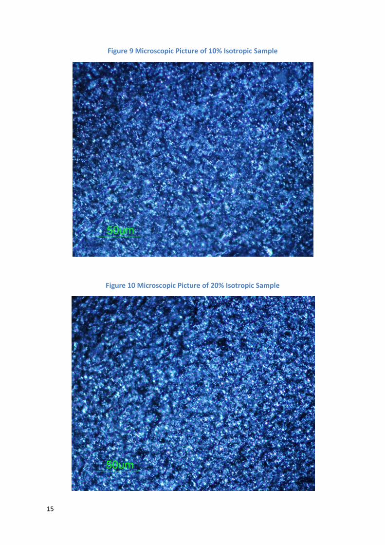
Pure Rubber, 10%, 20%, 30% Isotropic samples cured for 24 Hours at 25oC
The samples mixed for this testing regime were cured for 24 hours at 25oC as prescribed by
the manufacturer. The samples produced the stress-strain data shown in figures 11 and
table 4. Figure 8 below shows the structure of an isotropic sample loaded with 10% volume
CIP at a magnification factor of x20 using a microscope, the white flecks are CIP clusters.
This photograph shows that there is no order to the distribution of particles. Figure 9 shows
a 20% volume isotropic sample of the same magnification. From figure 9 it can be seen that
there is a higher density of white flecks and therefore CIP.
Cycle 1 Upload
Cycle 2-4 Upload
All Unload Parts
15
Figure 9 Microscopic Picture of 10% Isotropic Sample
Figure 10 Microscopic Picture of 20% Isotropic Sample
16
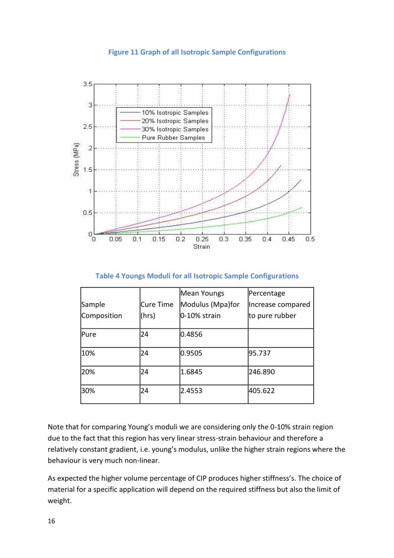
Figure 11 Graph of all Isotropic Sample Configurations
Table 4 Youngs Moduli for all Isotropic Sample Configurations
Sample
Composition
Cure Time
(hrs)
Mean Youngs
Modulus (Mpa)for
0-10% strain
Percentage
Increase compared
to pure rubber
Pure 24 0.4856
10% 24 0.9505 95.737
20% 24 1.6845 246.890
30% 24 2.4553 405.622
Note that for comparing Young’s moduli we are considering only the 0-10% strain region
due to the fact that this region has very linear stress-strain behaviour and therefore a
relatively constant gradient, i.e. young’s modulus, unlike the higher strain regions where the
behaviour is very much non-linear.
As expected the higher volume percentage of CIP produces higher stiffness’s. The choice of
material for a specific application will depend on the required stiffness but also the limit of
weight.
17
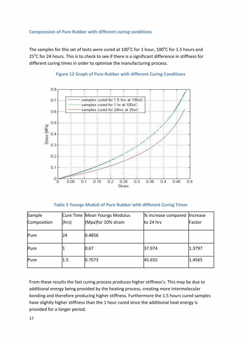
Compression of Pure Rubber with different curing conditions
The samples for this set of tests were cured at 100oC for 1 hour, 100oC for 1.5 hours and
25oC for 24 hours. This is to check to see if there is a significant difference in stiffness for
different curing times in order to optimize the manufacturing process.
Figure 12 Graph of Pure Rubber with different Curing Conditions
Table 5 Youngs Moduli of Pure Rubber with different Curing Times
Sample
Composition
Cure Time
(hrs)
Mean Youngs Modulus
(Mpa)for 10% strain
% increase compared
to 24 hrs
Increase
Factor
Pure 24 0.4856
Pure 1 0.67 37.974 1.3797
Pure 1.5 0.7073 45.655 1.4565
From these results the fast curing process produces higher stiffness’s. This may be due to
additional energy being provided by the heating process, creating more intermolecular
bonding and therefore producing higher stiffness. Furthermore the 1.5 hours cured samples
have slightly higher stiffness than the 1 hour cured since the additional heat energy is
provided for a longer period.
18
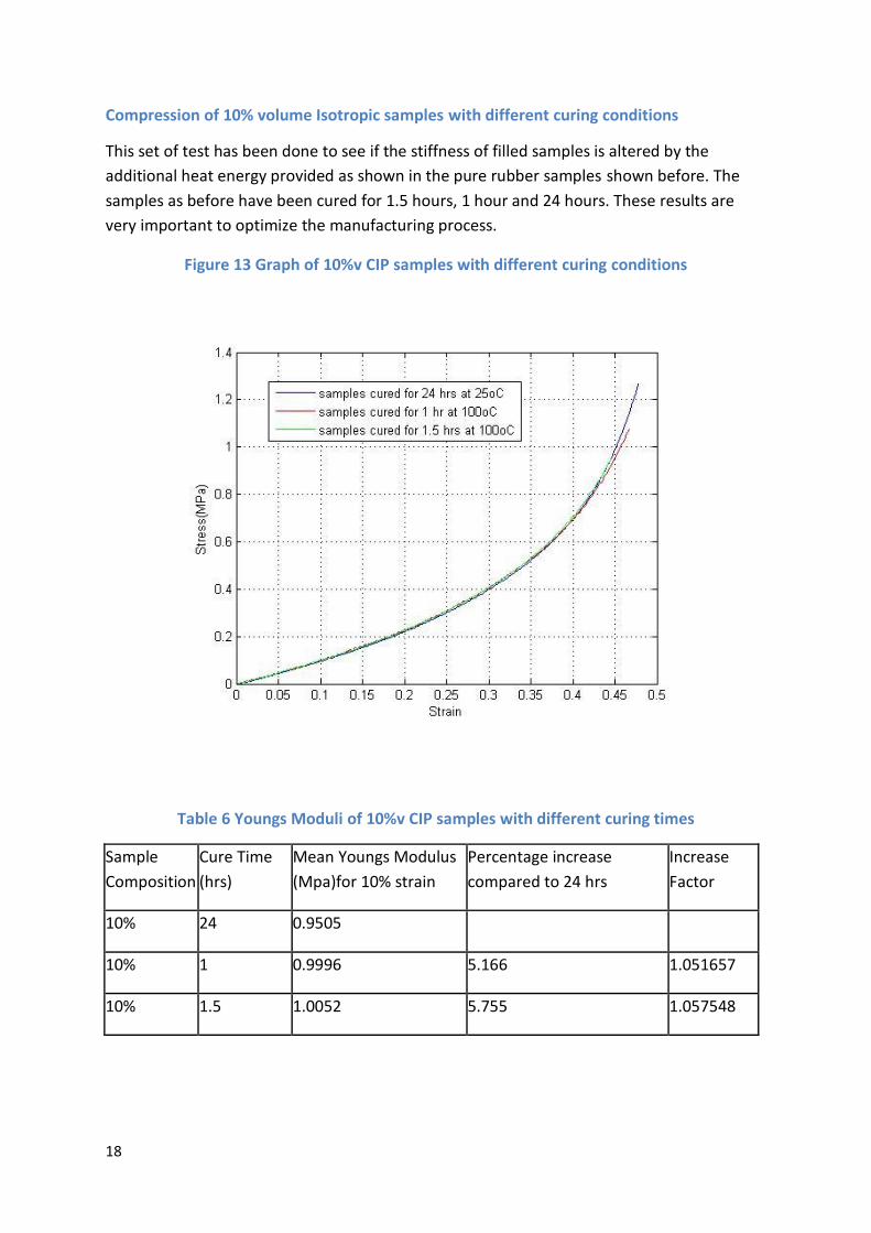
Compression of 10% volume Isotropic samples with different curing conditions
This set of test has been done to see if the stiffness of filled samples is altered by the
additional heat energy provided as shown in the pure rubber samples shown before. The
samples as before have been cured for 1.5 hours, 1 hour and 24 hours. These results are
very important to optimize the manufacturing process.
Figure 13 Graph of 10%v CIP samples with different curing conditions
Table 6 Youngs Moduli of 10%v CIP samples with different curing times
Sample
Composition
Cure Time
(hrs)
Mean Youngs Modulus
(Mpa)for 10% strain
Percentage increase
compared to 24 hrs
Increase
Factor
10% 24 0.9505
10% 1 0.9996 5.166 1.051657
10% 1.5 1.0052 5.755 1.057548
19
From these results it can be seen that the addition of heat has very little affect on the
stiffness of the samples, there is only a 5% increase in stiffness. Therefore unlike the pure
rubber there is only a small amount of additional bonding caused by the additional energy
provided. This means that the interaction between the filler and the matrix does not allow
for strengthening of the matrix, it can therefore be assumed that most of the heat energy is
absorbed by the CIP particles. This may be due to a higher thermal conductivity. From these
results all future samples will be cured for 1 hour at 100oC.
Compression of 10%, 20% and 30% Anisotropic samples
These samples have been cured for 1 hour at 100oC under a magnetic field of 400mT. This
field strength was used mainly because the amplifier being used overloads after time while
high currents are used. The value of 400mT was a safe magnetic field density that could be
achieved for the full curing time needed. Furthermore other studies (VARGA [4]) have
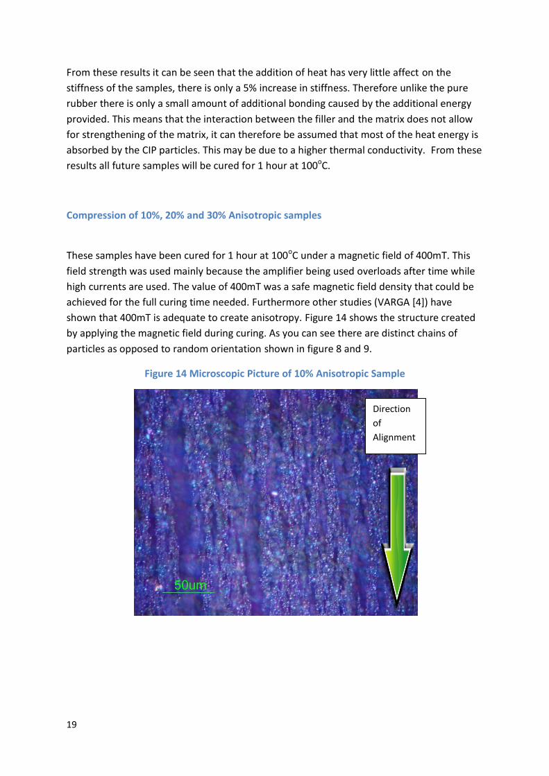
shown that 400mT is adequate to create anisotropy. Figure 14 shows the structure created
by applying the magnetic field during curing. As you can see there are distinct chains of
particles as opposed to random orientation shown in figure 8 and 9.
Figure 14 Microscopic Picture of 10% Anisotropic Sample
Direction
of
Alignment
20
There have been some problems with the compression tests for this anisotropic structure.
The rubber samples when compressed actually buckled which is not supposed to happen
the rubber should remain at a constant volume and therefore the diameter of the sample
should increase with decreasing height. Figure 15and 16 shows one of the samples as it
buckles.
The result from this buckling is a very steep upload at the beginning of the cycle then it
flattens out. Interestingly this behaviour is very consisitent for all the samples. At first it was
suspected that because the moulds between the poles of the electromagnet were not
completely covered by the pole and it was thought that the flux density would be weaker at
the edge of the poles.
To stop this only one mould at a time was cured between the magnetic poles. Unfortunately
this did not solve the problem. It was then discovered that the moulds that were being used
had deformed due to the heat and pressure of the curing process. New top plates were
manufactured with additional screw holes for extra security. Unfortunately this still did not
stop the buckling. It may be that the shear modulus is much less than the compressive
modulus. In order to stop the buckling occurring, the film of oil on the sample during testing
was removed. This did stop the buckling but unfortunately this causes additional friction on
the sample during testing which means that the force displacement will not be comparable
with the other tests. The test results are shown in figure 14 and table 7, but it must be
stated that these results will not be an accurate representation of the anisotropic samples.
Figure 15 Buckling Samples
21
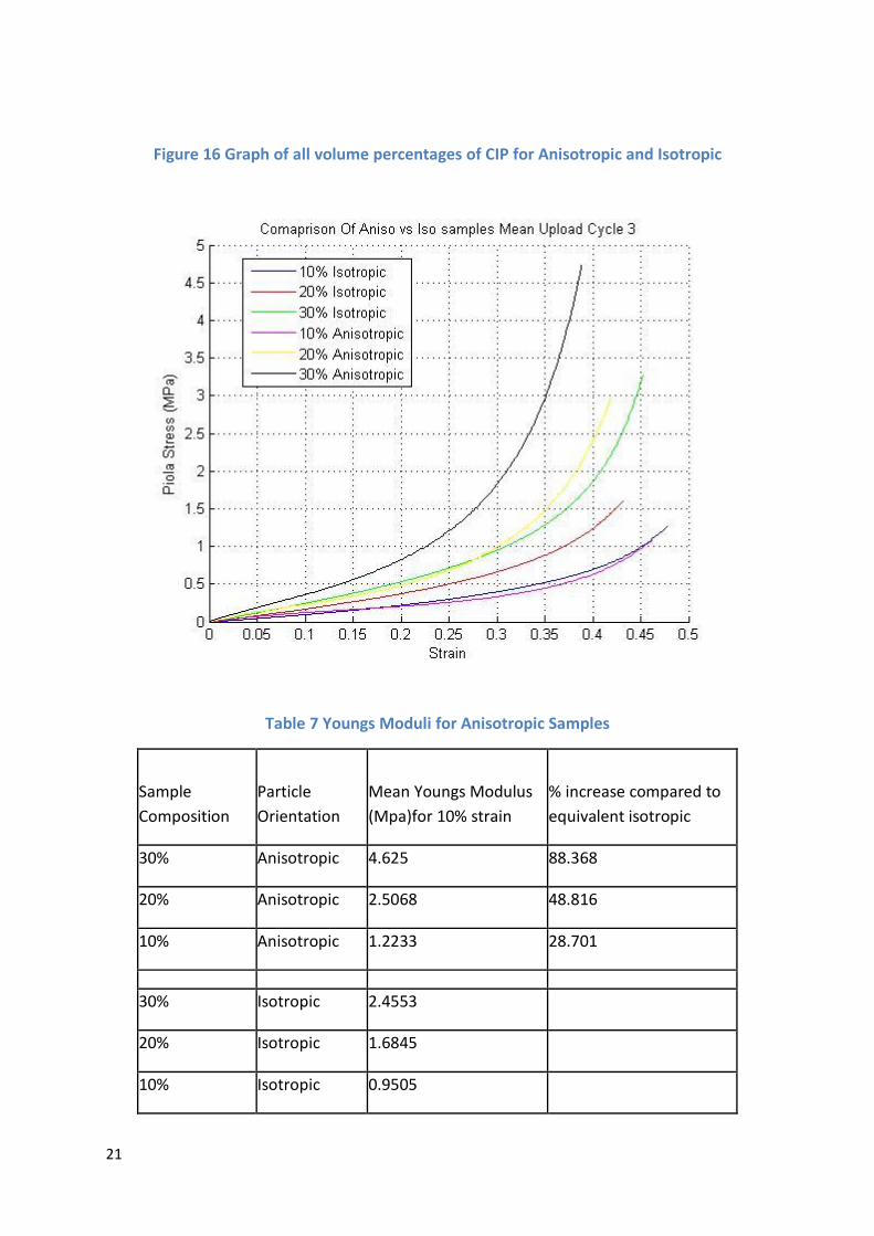
Table 7 Youngs Moduli for Anisotropic Samples
Sample
Composition
Particle
Orientation
Mean Youngs Modulus
(Mpa)for 10% strain
% increase compared to
equivalent isotropic
30% Anisotropic 4.625 88.368
20% Anisotropic 2.5068 48.816
10% Anisotropic 1.2233 28.701
30% Isotropic 2.4553
20% Isotropic 1.6845
10% Isotropic 0.9505
Figure 16 Graph of all volume percentages of CIP for Anisotropic and Isotropic structures
22
Interestingly it can be seen that the higher percentages of CIP produce larger increases in
the Young’s modulus. This will be due to denser particle chains created by the magnetic
field. The higher concentration of ferromagnetic elements will create a higher magnetic flux
density within the samples when curing, meaning that the individual particles will be
magnetically attracted towards each other creating thicker and longer chains.
Due to the fact that buckling is a factor in the testing of Anisotropic samples, it may be more
poignant to perform tensile tests instead of compression to discover the mechanical
properties that Anisotropy creates.
Compression of 10%, 20% and 30%, Anisotropic and Isotropic Samples with applied
magnetic fields
This set of tests will deal with the effect of applying a magnetic field through the samples
while being compressed. The magnetic field should increase the stiffness of the samples and
the higher volume percentages should produce a bigger MR effect. Furthermore the
Anisotropic samples should produce a bigger increase compared to the Isotropic samples.
The increase in stiffness is caused by the interaction of the magnetic particles in the matrix.
The magnetic flux causes a magnetic dipole interaction between every particle in the matrix.
In the Anisotropic samples the magnetic particles will be closer together, thereby increasing
the attractive force between them as attractive force is a function of distance.
23
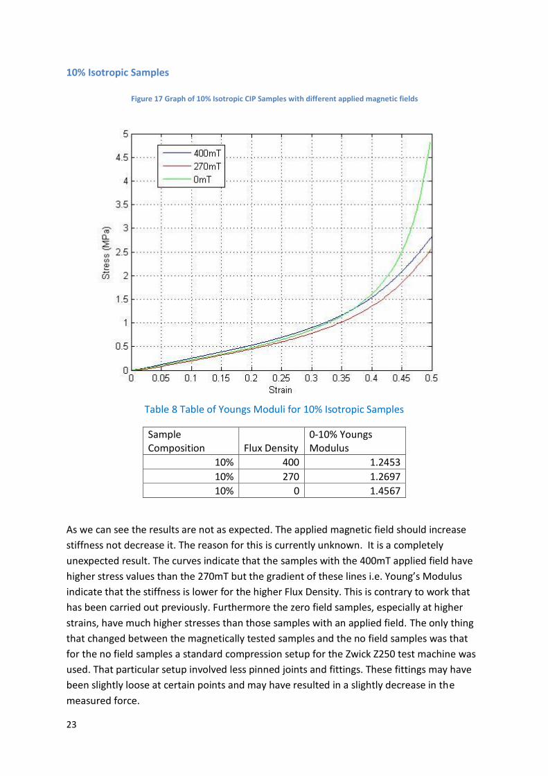
10% Isotropic Samples
Table 8 Table of Youngs Moduli for 10% Isotropic Samples
Sample Composition Flux Density
0-10% Youngs Modulus
10% 400 1.2453
10% 270 1.2697
10% 0 1.4567
As we can see the results are not as expected. The applied magnetic field should increase
stiffness not decrease it. The reason for this is currently unknown. It is a completely
unexpected result. The curves indicate that the samples with the 400mT applied field have
higher stress values than the 270mT but the gradient of these lines i.e. Young’s Modulus
indicate that the stiffness is lower for the higher Flux Density. This is contrary to work that
has been carried out previously. Furthermore the zero field samples, especially at higher
strains, have much higher stresses than those samples with an applied field. The only thing
that changed between the magnetically tested samples and the no field samples was that
for the no field samples a standard compression setup for the Zwick Z250 test machine was
used. That particular setup involved less pinned joints and fittings. These fittings may have
been slightly loose at certain points and may have resulted in a slightly decrease in the
measured force.
Figure 17 Graph of 10% Isotropic CIP Samples with different applied magnetic fields
24
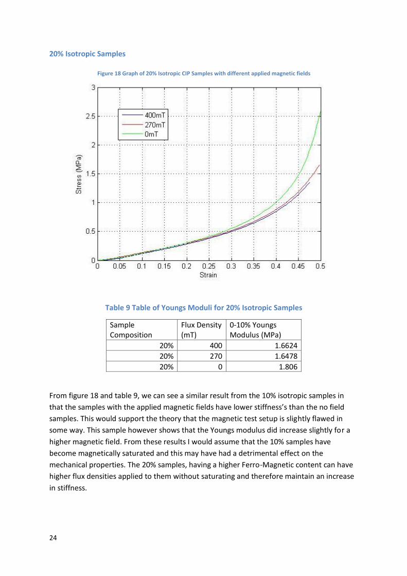
20% Isotropic Samples
Table 9 Table of Youngs Moduli for 20% Isotropic Samples
Sample Composition
Flux Density (mT)
0-10% Youngs Modulus (MPa)
20% 400 1.6624
20% 270 1.6478
20% 0 1.806
From figure 18 and table 9, we can see a similar result from the 10% isotropic samples in
that the samples with the applied magnetic fields have lower stiffness’s than the no field
samples. This would support the theory that the magnetic test setup is slightly flawed in
some way. This sample however shows that the Youngs modulus did increase slightly for a
higher magnetic field. From these results I would assume that the 10% samples have
become magnetically saturated and this may have had a detrimental effect on the
mechanical properties. The 20% samples, having a higher Ferro-Magnetic content can have
higher flux densities applied to them without saturating and therefore maintain an increase
in stiffness.
Figure 18 Graph of 20% Isotropic CIP Samples with different applied magnetic fields
25
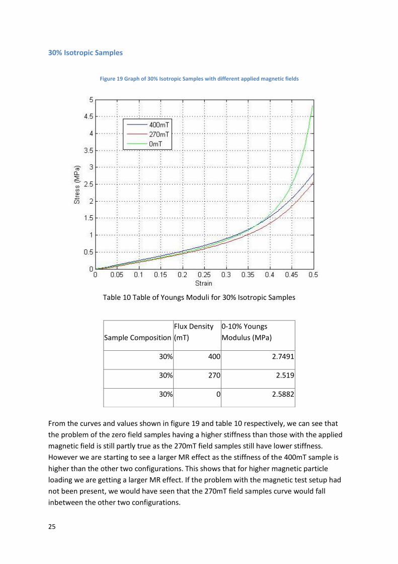
30% Isotropic Samples
Table 10 Table of Youngs Moduli for 30% Isotropic Samples
From the curves and values shown in figure 19 and table 10 respectively, we can see that
the problem of the zero field samples having a higher stiffness than those with the applied
magnetic field is still partly true as the 270mT field samples still have lower stiffness.
However we are starting to see a larger MR effect as the stiffness of the 400mT sample is
higher than the other two configurations. This shows that for higher magnetic particle
loading we are getting a larger MR effect. If the problem with the magnetic test setup had
not been present, we would have seen that the 270mT field samples curve would fall
inbetween the other two configurations.
Sample Composition
Flux Density
(mT)
0-10% Youngs
Modulus (MPa)
30% 400 2.7491
30% 270 2.519
30% 0 2.5882
Figure 19 Graph of 30% Isotropic Samples with different applied magnetic fields
26
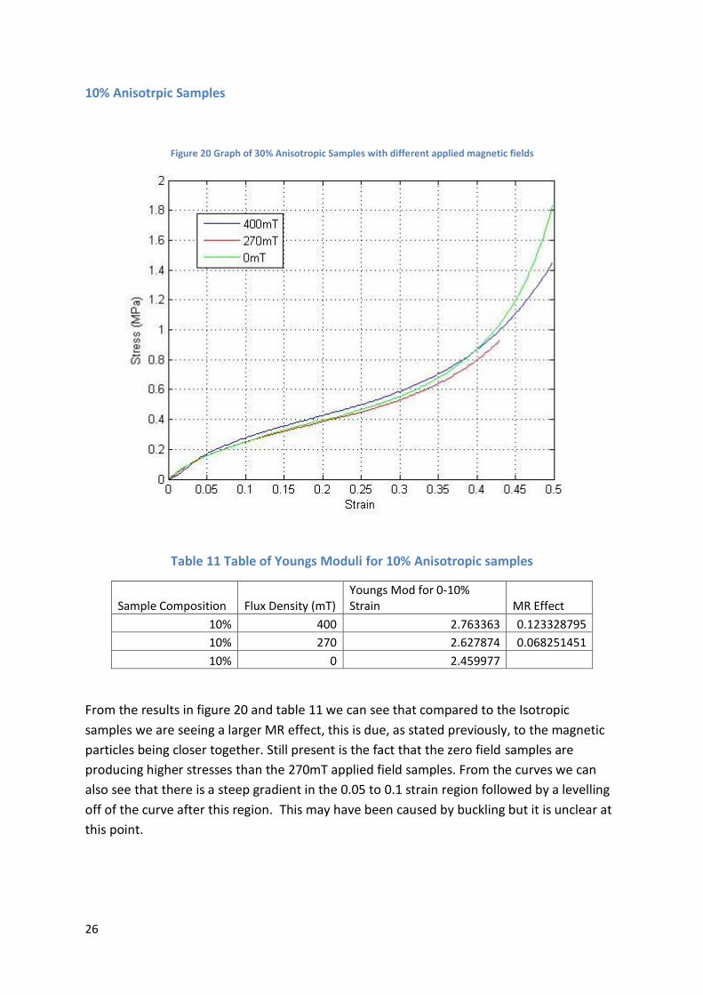
10% Anisotrpic Samples
Table 11 Table of Youngs Moduli for 10% Anisotropic samples
Sample Composition Flux Density (mT) Youngs Mod for 0-10% Strain MR Effect
10% 400 2.763363 0.123328795
10% 270 2.627874 0.068251451
10% 0 2.459977
From the results in figure 20 and table 11 we can see that compared to the Isotropic
samples we are seeing a larger MR effect, this is due, as stated previously, to the magnetic
particles being closer together. Still present is the fact that the zero field samples are
producing higher stresses than the 270mT applied field samples. From the curves we can
also see that there is a steep gradient in the 0.05 to 0.1 strain region followed by a levelling
off of the curve after this region. This may have been caused by buckling but it is unclear at
this point.
Figure 20 Graph of 30% Anisotropic Samples with different applied magnetic fields
27
20% Anisotropic Samples
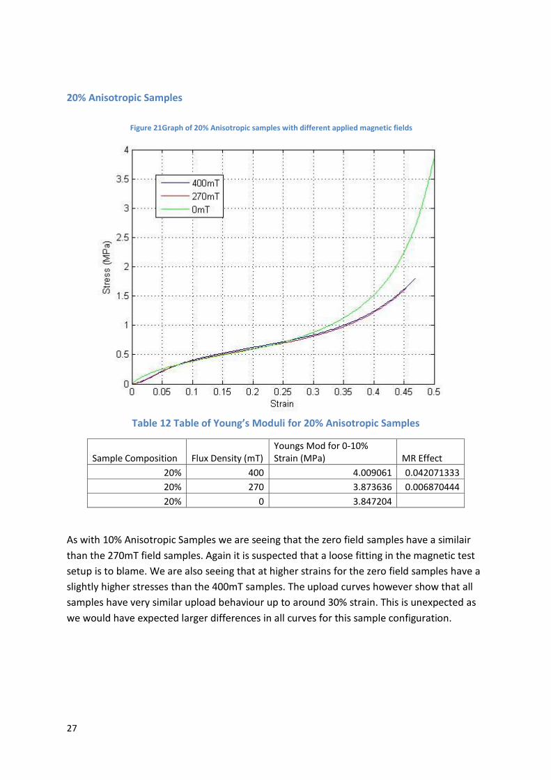
Table 12 Table of Young’s Moduli for 20% Anisotropic Samples
Sample Composition Flux Density (mT) Youngs Mod for 0-10% Strain (MPa) MR Effect
20% 400 4.009061 0.042071333
20% 270 3.873636 0.006870444
20% 0 3.847204
As with 10% Anisotropic Samples we are seeing that the zero field samples have a similair
than the 270mT field samples. Again it is suspected that a loose fitting in the magnetic test
setup is to blame. We are also seeing that at higher strains for the zero field samples have a
slightly higher stresses than the 400mT samples. The upload curves however show that all
samples have very similar upload behaviour up to around 30% strain. This is unexpected as
we would have expected larger differences in all curves for this sample configuration.
Figure 21Graph of 20% Anisotropic samples with different applied magnetic fields
28
30% Anisotropic Samples
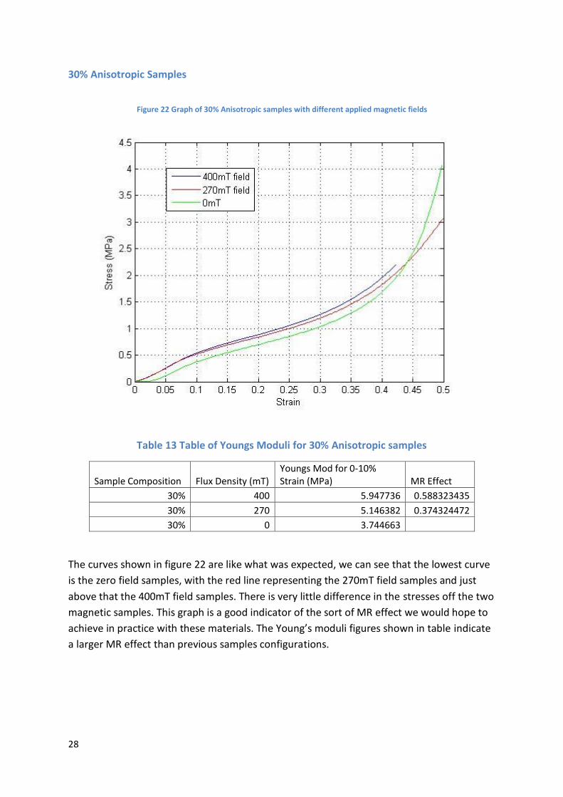
Table 13 Table of Youngs Moduli for 30% Anisotropic samples
Sample Composition Flux Density (mT) Youngs Mod for 0-10% Strain (MPa) MR Effect
30% 400 5.947736 0.588323435
30% 270 5.146382 0.374324472
30% 0 3.744663
The curves shown in figure 22 are like what was expected, we can see that the lowest curve
is the zero field samples, with the red line representing the 270mT field samples and just
above that the 400mT field samples. There is very little difference in the stresses off the two
magnetic samples. This graph is a good indicator of the sort of MR effect we would hope to
achieve in practice with these materials. The Young’s moduli figures shown in table indicate
a larger MR effect than previous samples configurations.
Figure 22 Graph of 30% Anisotropic samples with different applied magnetic fields
29
Modelling of MREs
In this report the modelling of the Isotropic samples will be concentrated on. The main
reason is the experimental problems with the anisotropic samples which need to be solved
first. I am using for analysis the Abaqus 6.8 Student Edition. Already implemented models
for rubber-like materials are the Neo-Hookean, the Mooney-Rivlin and the Ogden Model
which are all models for isotropic materials. Modelling an anisotropic material would
require a user defined constitutive equation using UMAT. This would go beyond the scope
of this report. A further assumption of the said implemented models is that the materials
are fully incompressible i.e. the volume does not change during deformation and the
poisson ratio is 0.5. Furthermore G the shear modulus is related to the Elastic modulus E by
the equation, , but this is only valid on the linear theory ,i.e. in the small strain
region.
The standard hyper elastic models which will be used are the, Neo-Hookean and Mooney
Rivlin. All these models are derived from the standard Ogden model shown in Equation 2.
This model is based on the relationship between the Strain Energy Function9 and the
principal stretch ratios.
Equation 2 Standard Ogden Model
Where is the strain energy and , are the principal stretch ratios for each
direction. is defined as the shear modulus, and is a material constant.
The Mooney Rivlin model is obtained by setting N=2, = 2, = -2. This produces Equation
3 shown below.
Equation 3 Standard Mooney Rivlin Model
Where c10
, c01
, and the shear modulus is µ =
The Neo-Hookean model is derived from the standard Ogden model by setting N=1, = 2,
this results in Equation 4.
Equation 4 Standard Neo Hookean Model
9 Equations from Non-Linear Solid Mechanics by Gerhard A Holzapfel
30
Where c1
and the shear modulus is
The Young’s modulus can be calculated from the coefficients calculated by Abaqus shown by
these equations:
These constitutive model need to be fitted to experimental data to calculate the model
parameters. This fitting will be done by Abaqus using a least square method. To get an idea
of the suitability of the fit a coefficient of determination R2 will be calculated. This
coefficient is often used in statistics. It approaches 1 the better the fit, a value of 0 would
mean the fit is useless.
exp fitres
22
2
2
1 ... nresresresnorm
i
itotS 2exp
_
exp, )(
tot
tot
S
normSR
2
2
Where res are the residuals, norm is the 2-Norm also known as the Euclidian length of the residuals, Stot is the sum of squares and finally R2 is the coefficient of determination.
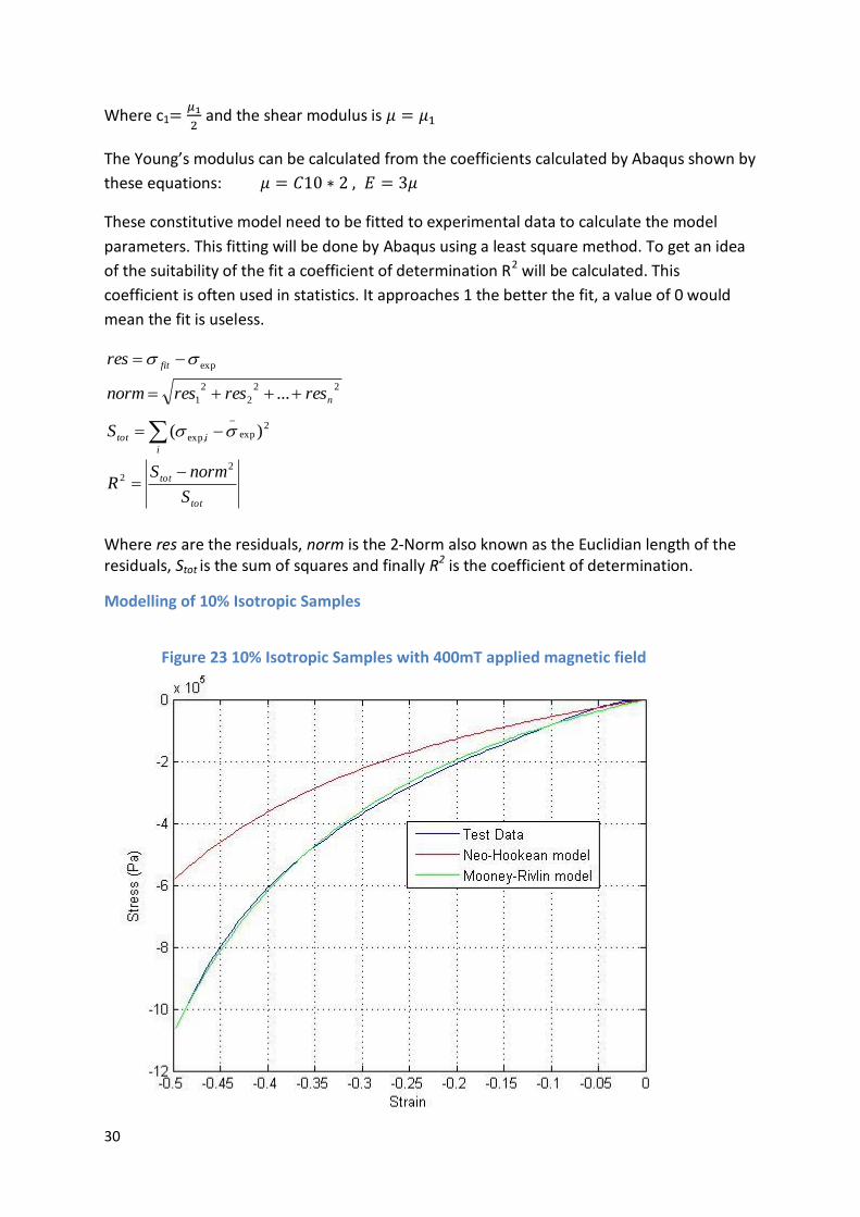
Modelling of 10% Isotropic Samples
Figure 23 10% Isotropic Samples with 400mT applied magnetic field
31
Coefficients for 10% Isotropic samples with 400mT applied magnetic field
HYPERELASTICITY - MOONEY-RIVLIN STRAIN ENERGY
D1 C10 C01
0.000000 84061.8510 34812.0823
HYPERELASTICITY - NEO-HOOKEAN STRAIN ENERGY
D1 C10 C01
0.00000 83567.7120 0.00000000
Coefficients for 10% Isotropic Samples with 270mT applied magnetic field
HYPERELASTICITY - MOONEY-RIVLIN STRAIN ENERGY
D1 C10 C01
0.00000000 120041.678 18855.2399
HYPERELASTICITY - NEO-HOOKEAN STRAIN ENERGY
D1 C10 C01
0.00000000 145569.612 0.00000000
Figure 24 10% Isotropic Samples with 270mT applied magnetic field
32
Coefficients for 10% Isotropic Samples with no applied magnetic field
HYPERELASTICITY - MOONEY-RIVLIN STRAIN ENERGY
D1 C10 C01
0.00000000 62757.9238 78950.0356
HYPERELASTICITY - NEO-HOOKEAN STRAIN ENERGY
D1 C10 C01
0.00000000 172278.547 0.00000000
Figure 25 10% Isotropic samples no applied magnetic field
33
From Figure 23 we can see that the best model fit is the Mooney-Rivlin. This was confirmed
by the R2 coefficient which was calculated as 0.9988 for the Mooney-Rivlin and 0.5558 for
the Neo-Hookean.
From Figure 24 we can see that both models are quite good for most strain levels. The R2
coefficient for the Mooney Rivlin model the R2 value was 0.9987 and for the Neo-Hookean
model R2 is 0.9902. this shows that the Mooney-Rivlin is still the better fit for this material
configuration with and without magnetic fields.
From Figure 25 we can also see that the Mooney Rivlin model is still the best fit, and the R2
values confirm this as they are 0.9917 for the Mooney-Rivlin and 0.9231 for the Neo-
Hookean. Finally the Mooney-Rivlin Model is the best fit for this material tested with and
without magnetic field. Using the coefficients shown previously Table 14 and Table 15 were
constructed to show the differences in the Young’s moduli from test data and coefficients.
Table 14 Table of Coefficients for Mooney-Rivlin Model
Samples Composition
Applied Field (mT)
C10 Coefficient
C01 Coefficient
Shear Modulus (MPa)
Youngs Modulus (MPa)
Youngs Modulus form test data (MPa)
10% 400 84061.851 34812.0823 0.2377 0.7132 1.2453
10% 270 120041.67 18855.2399 0.2778 0.8334 1.2697
10% 0 62757.923 78950.0356 0.2834 0.8502 1.4567
Table 15 Table of Coefficients for Neo-Hookean Model
Samples Composition
Applied Field (mT)
C10 Coefficient
Shear Modulus (MPa)
Youngs Modulus (MPa)
Youngs Modulus form test data (MPa)
10% 400 83567.7120 0.1671 0.5014 1.2453
10% 270 145569.6120 0.2911 0.8734 1.2697
10% 0 172278.5470 0.3446 1.0337 1.4567
34
Modelling of 20% Isotropic Samples
Figure 26 20% Isotropic Sample with 400mT applied magnetic field
Coefficients for 20% Isotropic Samples with 400mT applied magnetic field
HYPERELASTICITY - MOONEY-RIVLIN STRAIN ENERGY
D1 C10 C01
0.00000000 95259.1322 61905.0798
HYPERELASTICITY - NEO-HOOKEAN STRAIN ENERGY
D1 C10 C01
0.00000000 89553.1134 0.00000
35
Coefficients for 20% Isotropic Samples with 270mT applied magnetic field
HYPERELASTICITY - MOONEY-RIVLIN STRAIN ENERGY
D1 C10 C01
0.00000000 128736.268 48048.7121
HYPERELASTICITY - NEO-HOOKEAN STRAIN ENERGY
D1 C10 C01
0.00000000 192142.047 0.00000000
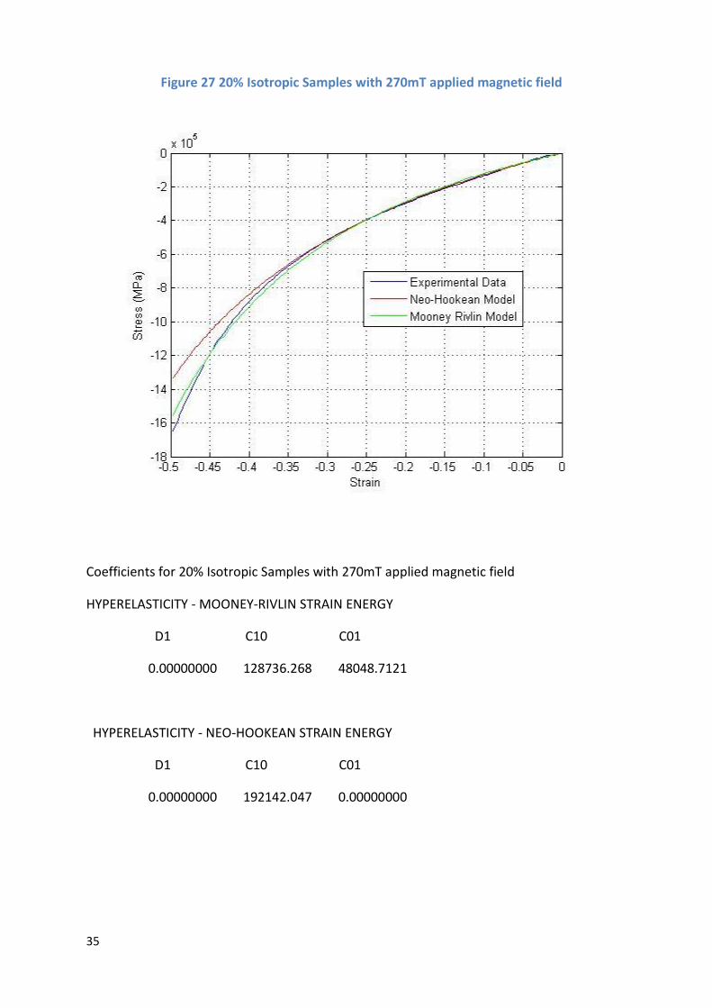
Figure 27 20% Isotropic Samples with 270mT applied magnetic field
36
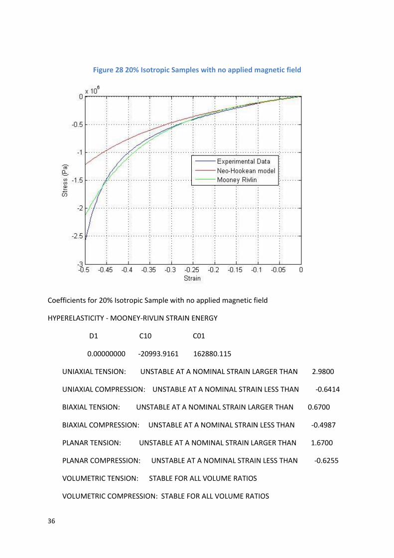
Figure 28 20% Isotropic Samples with no applied magnetic field
Coefficients for 20% Isotropic Sample with no applied magnetic field
HYPERELASTICITY - MOONEY-RIVLIN STRAIN ENERGY
D1 C10 C01
0.00000000 -20993.9161 162880.115
UNIAXIAL TENSION: UNSTABLE AT A NOMINAL STRAIN LARGER THAN 2.9800
UNIAXIAL COMPRESSION: UNSTABLE AT A NOMINAL STRAIN LESS THAN -0.6414
BIAXIAL TENSION: UNSTABLE AT A NOMINAL STRAIN LARGER THAN 0.6700
BIAXIAL COMPRESSION: UNSTABLE AT A NOMINAL STRAIN LESS THAN -0.4987
PLANAR TENSION: UNSTABLE AT A NOMINAL STRAIN LARGER THAN 1.6700
PLANAR COMPRESSION: UNSTABLE AT A NOMINAL STRAIN LESS THAN -0.6255
VOLUMETRIC TENSION: STABLE FOR ALL VOLUME RATIOS
VOLUMETRIC COMPRESSION: STABLE FOR ALL VOLUME RATIOS
37
HYPERELASTICITY - NEO-HOOKEAN STRAIN ENERGY
D1 C10 C01
0.00000000 174917.522 0.00000000
From Figure 26 we can see that again the Mooney-Rivlin Model is the best fit for this sample
configuration. This is confirmed with the R2 coefficient being 0.9987 for the Mooney-Rivlin
and 0.2354 for the Neo-Hookean.
Figure 27 shows that for lower strains both models are quite accurate but as strain increases
the Neo-Hookean curve starts to move away from the test data. The Mooney-Rivlin is still
the best model for this material. Furthermore this is confirmed with the R2 coefficient, it is
0.9970 for the Mooney-Rivlin and 0.9671 for the Neo-Hookean.
In Figure 28 we are starting to see a few discrepancies between the Mooney-Rivlin model
and the test data especially at higher strains. Even so the Mooney-Rivlin is still the best
fitting model for this data as shown again by the R2 coefficient. For the Mooney-Rivlin R2 is
0.9827 and for the Neo-Hookean R2 is 0.7041. Unusually the Abaqus has stated the
Mooney-Rivlin Model as unstable.
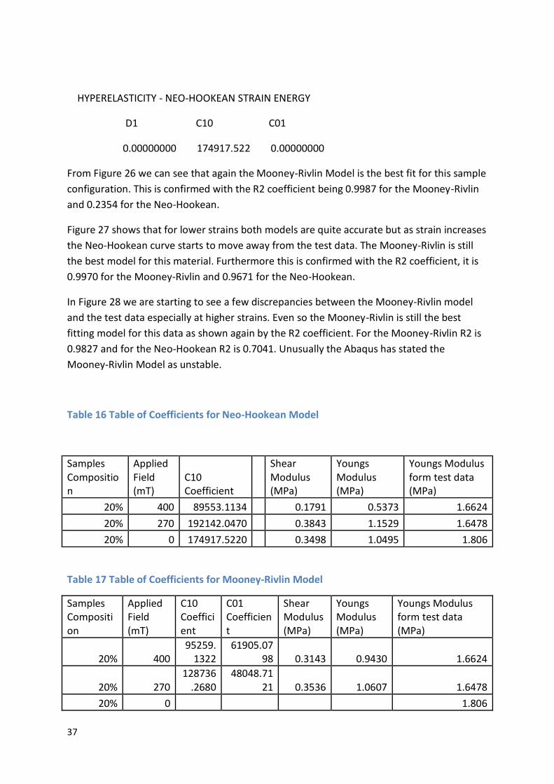
Table 16 Table of Coefficients for Neo-Hookean Model
Samples Composition
Applied Field (mT)
C10 Coefficient
Shear Modulus (MPa)
Youngs Modulus (MPa)
Youngs Modulus form test data (MPa)
20% 400 89553.1134 0.1791 0.5373 1.6624
20% 270 192142.0470 0.3843 1.1529 1.6478
20% 0 174917.5220 0.3498 1.0495 1.806
Table 17 Table of Coefficients for Mooney-Rivlin Model
Samples Composition
Applied Field (mT)
C10 Coefficient
C01 Coefficient
Shear Modulus (MPa)
Youngs Modulus (MPa)
Youngs Modulus form test data (MPa)
20% 400 95259.
1322 61905.07
98 0.3143 0.9430 1.6624
20% 270 128736
.2680 48048.71
21 0.3536 1.0607 1.6478
20% 0 1.806

38
Modelling of 30% Isotropic Samples
Coefficients for 30% Isotropic Samples with 400mT applied magnetic field
HYPERELASTICITY - MOONEY-RIVLIN STRAIN ENERGY
D1 C10 C01
0.00000000 265354.405 59029.5065
HYPERELASTICITY - NEO-HOOKEAN STRAIN ENERGY
D1 C10 C01
0.00000000 352369.597 0.00000000
Figure 29 30% Isotropic Samples with 400mT applied magnetic field
39
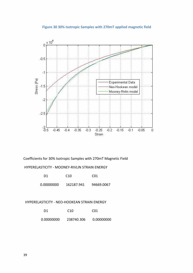
Coefficients for 30% Isotropic Samples with 270mT Magnetic Field
HYPERELASTICITY - MOONEY-RIVLIN STRAIN ENERGY
D1 C10 C01
0.00000000 162187.941 94669.0067
HYPERELASTICITY - NEO-HOOKEAN STRAIN ENERGY
D1 C10 C01
0.00000000 238740.306 0.00000000
Figure 30 30% Isotropic Samples with 270mT applied magnetic field
40
Coefficients for 30% Isotropic Samples with no applied magnetic field
HYPERELASTICITY - MOONEY-RIVLIN STRAIN ENERGY
D1 C10 C01
0.00000000 -93284.8951 304559.773
***WARNING: UNSTABLE HYPERELASTIC MATERIAL
UNIAXIAL TENSION: UNSTABLE AT A NOMINAL STRAIN LARGER THAN 0.9500
UNIAXIAL COMPRESSION: UNSTABLE AT A NOMINAL STRAIN LESS THAN -0.4513
BIAXIAL TENSION: UNSTABLE AT A NOMINAL STRAIN LARGER THAN 0.3500
BIAXIAL COMPRESSION: UNSTABLE AT A NOMINAL STRAIN LESS THAN -0.2839
PLANAR TENSION: UNSTABLE AT A NOMINAL STRAIN LARGER THAN 0.7200
PLANAR COMPRESSION: UNSTABLE AT A NOMINAL STRAIN LESS THAN -0.4186
VOLUMETRIC TENSION: STABLE FOR ALL VOLUME RATIOS
VOLUMETRIC COMPRESSION: STABLE FOR ALL VOLUME RATIOS
Figure 31 30% Isotropic Samples with no applied field
41
HYPERELASTICITY - NEO-HOOKEAN STRAIN ENERGY
D1 C10 C01
0.00000000 325749.014 0.00000000
From these simulations we can see that the Mooney-Rivlin Model is a good model for the
samples where a magnetic field is present. However when there is no magnetic field present
this model becomes unstable. The R2 values for all the cycles are shown in Table 18. This
means that this model will have to be altered in order to be used for simulations. Table 19
and Table 20 show a comparison of the simulated young’s moduli to the calculated Modulus
from the test data.
Table 18 Table of R2 values for 30% Isotropic Samples
Samples Composition
Applied Field Strength (mT)
R2 for Mooney Rivlin
R2 for Neo-Hookean
30% 400 0.9964 0.9854
30% 270 0.9977 0.8139
30% 0 0.9496 0.3185
Table 19 Youngs Modulus for 30% Isotropic Samples for Neo-Hookean Model
Samples Composition
Applied Field (mT)
C10 Coefficient
Shear Modulus (MPa)
Youngs Modulus (MPa)
Youngs Modulus form test data (MPa)
30% 400 352369.5970 0.7047 2.1142 2.7491
30% 270 238740.3060 0.4775 1.4324 2.519
30% 0 325749.0140 0.6515 1.9545 2.5882
Table 20 Youngs Modulus for 30% Isotropic Samples for Mooney-Rivlin Model
Samples Composition
Applied Field (mT)
C10 Coefficient
C01 Coefficient
Shear Modulus (MPa)
Youngs Modulus (MPa)
Youngs Modulus from test data (MPa)
30% 400 265354.40
50 59029.506
5 0.6488 1.9463 2.7491
30% 270 162187.94
10 94669.006
7 0.5137 1.5411 2.519
30% 0 2.5882
42
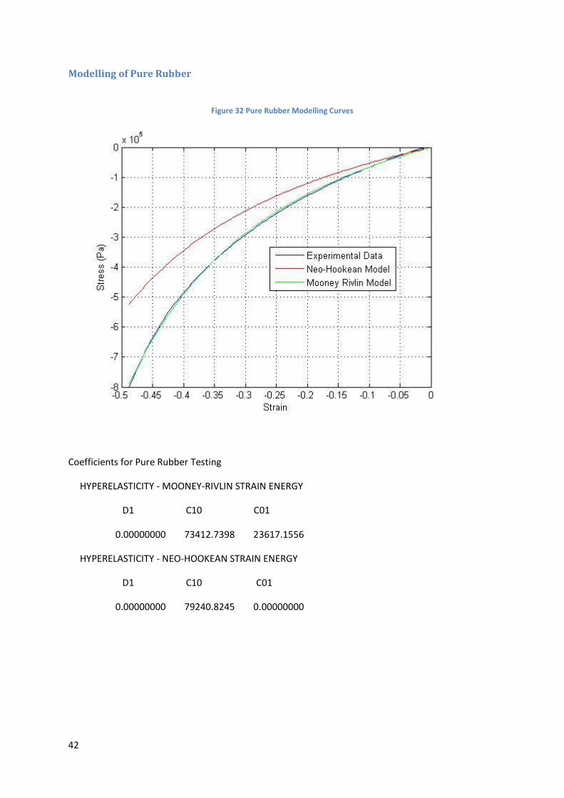
Modelling of Pure Rubber
Figure 32 Pure Rubber Modelling Curves
Coefficients for Pure Rubber Testing
HYPERELASTICITY - MOONEY-RIVLIN STRAIN ENERGY
D1 C10 C01
0.00000000 73412.7398 23617.1556
HYPERELASTICITY - NEO-HOOKEAN STRAIN ENERGY
D1 C10 C01
0.00000000 79240.8245 0.00000000
43
Table 21 Youngs Moduli for Pure Rubber for Mooney Rivlin Model
Samples Composition
Applied Field (mT)
C10 Coefficient
C01 Coefficient
Shear Modulus (MPa)
Youngs Modulus (MPa)
Youngs Modulus form test data (MPa)
Pure 0 73412.7398 23617.155 0.1941 0.5822 0.67
Table 22 Youngs Moduli for Pure Rubber Neo-Hookean model
Samples Composition
Applied Field (mT)
C10 Coefficient
Shear Modulus (MPa)
Youngs Modulus (MPa)
Youngs Modulus form test data (MPa)
Pure 0 79240.8245 0.1585 0.4754 0.67
The pure rubber is like all the rest of the samples that have been modelled in that the best fit is with
the Mooney-Rivlin model. The R2 values are 0.9995 for the Mooney-Rivlin model and 0.7656 for the
Neo-Hookean.
In conclusion it would appear that the best model for this material is the Mooney-Rivlin model, it has
consistently close to 1 R2 value providing a good fit.
Conclusions
The main conclusions of this report are that the manufacturing process has been optimized and now
all future samples will be cured for 1hrs at 100oC. Furthermore it is now possible to successfully
create Anisotropy within the MRE’s. Another main point from these set of test is that a method
whereby a magnetic field is passed through the sample while being compressed has been achieved.
Some of the problems that have occurred unexpectedly during these tests were the buckling of
anisotropic samples. This means that in future it would be best to test the anisotropic samples in
tension rather than compression. Unfortunately applying a magnetic field through the sample will be
difficult and a new test setup will have to be created.
Future work on this material will be carried out to create a general constitutive model, and to
achieve this task many more tests will have to be undertaken to fully define the MRE’s mechanical
properties.
44
Bibliography
[1] Gerlind Schuberts 1st Year Report
[2] M. Kallio Preliminary tests on an MRE device
[3] M. Farshad Magnetoactive elastomer composites [4] Z. Varga Magnetic Field Sensitive functional elastomers with tunable modulus
[5]Dr Philip Harrison, MRE Presentation
[6] Equations and Calculations are from Guide for rubber mixing process by Ms Gerlind Schubert [7 ] BS ISO 7742 Determination of Compression stress strain properties for Vulcanized
Rubbers
[8] Reference from (http://en.wikipedia.org/wiki/Mullins_effect) [9] Equations from Non-Linear Solid Mechanics by Gerhard A Holzapfel
[10]Picture from http://en.wikipedia.org/wiki/Solenoid
[11] Referenced from http://www.powerstream.com/Wire_Size.htm (AWG 23)
45
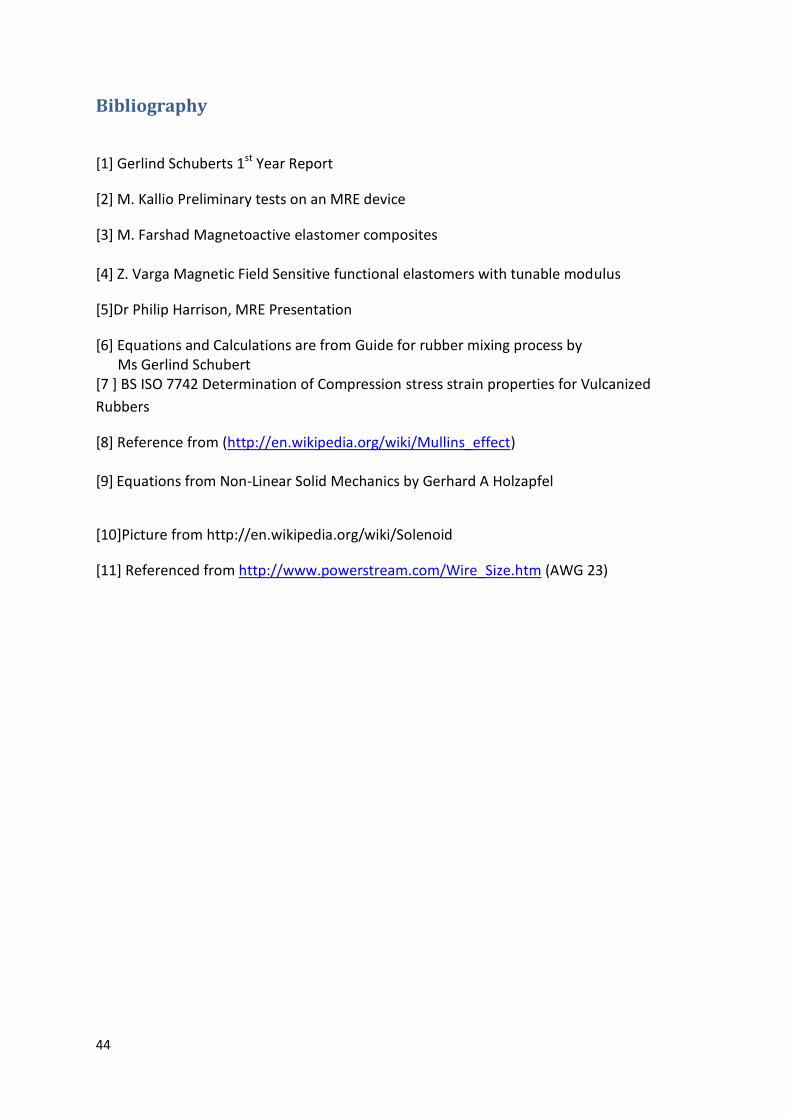
Appendix A : Calculation for Solenoids
First a target Magnetic Flux Density of B = 400 mTeslas was set. This is a relatively high magnetic
field but will be suitable for all experiments that need to be done. Furthermore the flux density can
be changed by altering the current supply. The max current that the power supply can safely
produce is 5A.
Figure A1[10]: A typical solenoid field. Lines represent magnetic field lines. “Dots” and “X’s” are coil
cross-section.
Figure A1 shows a wire coil in cross-section and the arrowed lines represent the magnetic field lines.
This shows that the field through a solenoid is very uniform and will be ideal for use when
compressing samples.
The basic equation for calculating the magnetic flux density at a inside the coil at a point away from
the ends is given as:
Where: B = magnetic flux density Unit is Tesla
µ = Kµ0 where k = relative permeability of core material and
µ0=magnetic constant and is the permeability of a vacuum
µ0= 4π x 10-7 unit is Tesla Metre per Ampere
N =number of turns L = length of solenoid
I = Current Unit is Amperes
10 Picture from http://en.wikipedia.org/wiki/Solenoid
46
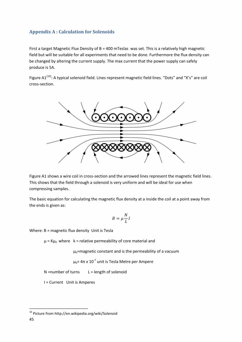
Therefore what is required to build this solenoid is the turns density N/L. With this the appropriate
coil can be designed and manufactured.
The core material is going to be air which has K=1
B (Tesla) I (Amperes) K µ (T.m/Ampere)
0.4 5 1 1.25664e-006
Therefore:
=1.5915e+006 turns/metre
As you can see this number is completely impractical. 1.5 million turns in one metre would
require a long amount of time to wind. Furthermore the wire diameter would be required to
be 6.2832e-004mm diameter and this diameter would not support the necessary current
required as specified by the American Wire Gauge. This gauge specifies that a wire will
carry a maximum current of 4.7 Amperes with a wire diameter of 0.57404mm[11].
For all the above reasons the idea of a solenoid to apply the magnetic field was rejected.
11 Referenced from http://www.powerstream.com/Wire_Size.htm (AWG 23)
47
Appendix B: Faulty test setup results
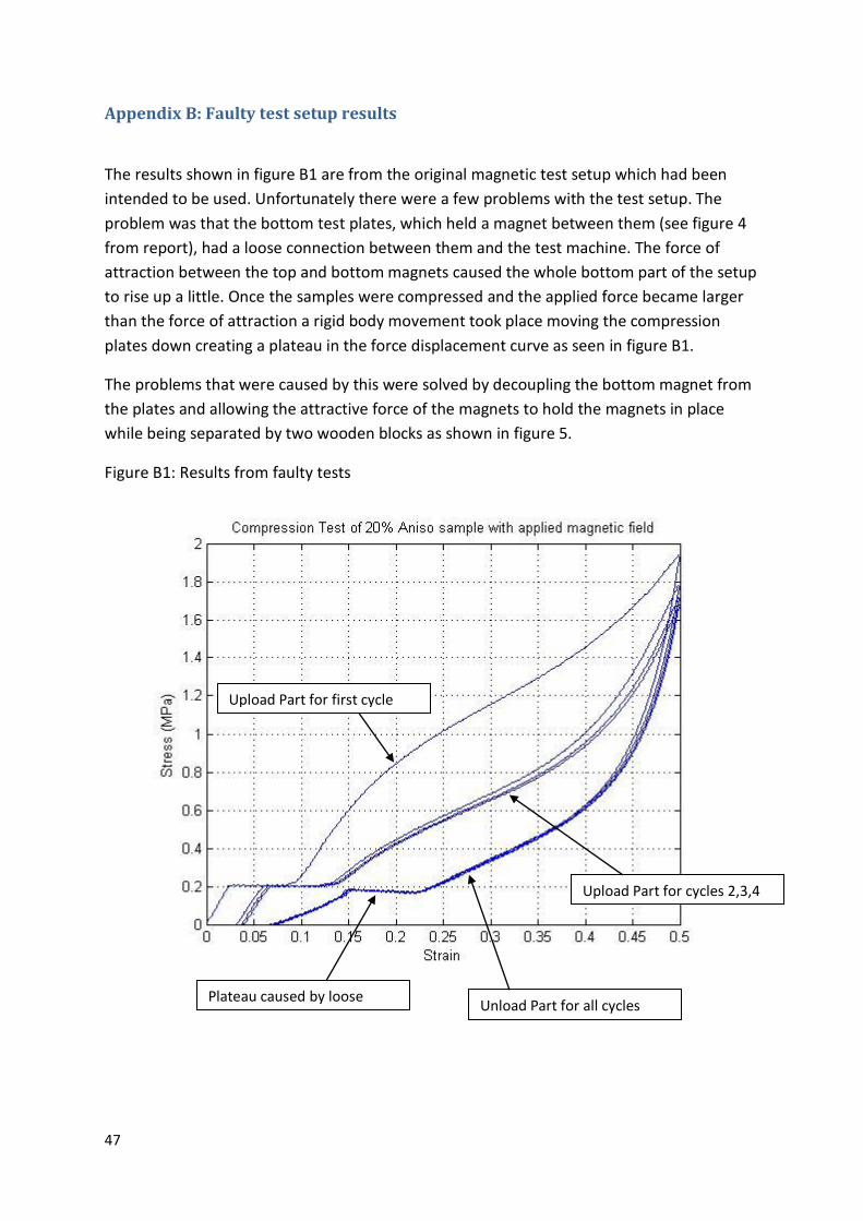
The results shown in figure B1 are from the original magnetic test setup which had been
intended to be used. Unfortunately there were a few problems with the test setup. The
problem was that the bottom test plates, which held a magnet between them (see figure 4
from report), had a loose connection between them and the test machine. The force of
attraction between the top and bottom magnets caused the whole bottom part of the setup
to rise up a little. Once the samples were compressed and the applied force became larger
than the force of attraction a rigid body movement took place moving the compression
plates down creating a plateau in the force displacement curve as seen in figure B1.
The problems that were caused by this were solved by decoupling the bottom magnet from
the plates and allowing the attractive force of the magnets to hold the magnets in place
while being separated by two wooden blocks as shown in figure 5.
Figure B1: Results from faulty tests
Unload Part for all cycles
Upload Part for first cycle
Upload Part for cycles 2,3,4
Plateau caused by loose
fitting