Embed Size (px)
Citation preview
UNIVERSITY OF GOTHENBURG Department of Earth Sciences Geovetarcentrum/Earth Science Centre
ISSN 1400-3821 B 597 Bachelor of Science thesis Göteborg 2010
Mailing address Address Telephone Telefax Geovetarcentrum Geovetarcentrum Geovetarcentrum 031-786 19 56 031-786 19 86 Göteborg University S 405 30 Göteborg Guldhedsgatan 5A S-405 30 Göteborg SWEDEN
Groundwater flow and quality in the vicinity of an
urbanised part of the Säveån stream, Gothenburg
Anna Lundgren
2
Groundwater flow and quality in the vicinity of an urbanised part
of the Säveån stream, Gothenburg
Abstract Before the Göta älv River meets the sea in Gothenburg many smaller streams have their outlet
in it, one of the larger is the Säveån stream. The urbanised hydrogeological environment is
complex and the need for a greater understanding of e.g. transportation pathways of water and
sediments and with them potential contaminants increases with the city’s development. One
important diffuse source of contaminants is the filling material which is present to large extent
in the central parts of Gothenburg, forming an upper unconfined aquifer. Thick clay layers in
the Gothenburg stratigraphy protect lower aquifers formed in glaciofluvial and till deposits to
large extent from these pollutants, but the hydrological contact between the filling material
and water bodies is of interest when mapping the spreading of urban contaminants.
Studies of the groundwaters inflow and outflow between an aquifer in filling material and the
Säveån stream was done in November 2009 in the central parts of Gothenburg to get a greater
understanding of contaminant pathways in an urbanised hydrogeological environment. The
flow rates were measured with a seepage meter and the results were linked to urban surfaces
in the area to interpret how they can affect the outflow of groundwater to the Säveån stream.
The measurements during the study period showed a greater outflow on the west side than on
the east side of the Säveån stream where also the urban surfaces are more permeable. PAH
and metal concentrations in the groundwater at the flow rate measuring sites were analysed at
different points and depths to get an appreciation of the concentration rates reaching the
Säveån stream through groundwater flow.
Keywords: urban hydrogeology, urban pollution pathways, groundwater flow, seepage meter,
Säveån, Functional Facies, DiPol project
Sammanfattning I Göteborg mynnar Göta älv ut i havet men innan dess har många mindre vattendrag sina
utlopp i den, där en av de större är Säveån. Den urbaniserade hydrogeologiska miljön är
komplex och behovet av förståelse av t.ex. transportvägar för vatten och sediment och med
dem potentiella föroreningar ökar tillsammans med stadens tillväxt. En viktig diffus källa till
föroreningar finns i fyllnadsmaterial som i stor utsträckning bildar en övre öppen akvifer i de
centrala delarna av Göteborg. Tjocka lerlager i Göteborgs stratigrafi gör att undre akviferer
utbildade i isälvsmaterial och morän i stor utsträckning är skyddade mot dessa föroreningar
men den hydrologiska kontakten mellan fyllnadsmaterialet och vattendragen är av intresse för
kartläggning av urban föroreningsspridning.
Studier av grundvattnets in- och utflöde mellan en akvifer i fyllnadsmaterial och Säveån har
utförts under november 2009 i centrala delar av Göteborg för att få en bättre förståelse av
föroreningars spridningsvägar i en urbaniserad hydrogeologisk miljö. Flödena mättes med en
seepage meter och resultaten har sedan kopplats samman med urbana ytor i området för att
tolka hur de kan påverkar utflödet av grundvatten till Säveån. Mätningarna under mätperioden
visade att det är ett större utflöde på västra sidan än på östra sidan om Säveån där de urbana
ytorna också är mer permeabla. PAH och metallkoncentrationer i grundvatten har analyserats
vid flödesmätningsstationerna vid olika punkter och djup för att få en uppfattning av vilka
koncentrationer som kan nå Säveån denna väg.
3
Table of contents
Table of contents ........................................................................................................................ 3
1. Introduction ............................................................................................................................ 5
1.1. Urban geology ................................................................................................................. 5
1.2. Project background .......................................................................................................... 5
1.3. The project goal ............................................................................................................... 6
1.4. The scope of the work ..................................................................................................... 6
2. Background theory ................................................................................................................. 6
2.1. Hydrology ........................................................................................................................ 6
2.1.1. The water balance equation ...................................................................................... 6
2.1.2. Stream hydrogeology ............................................................................................... 7
2.1.3 The hydrological year -What controls the water level? ............................................ 7
2.2. Chemistry ........................................................................................................................ 8
2.2.1. Chemistry of natural waters ..................................................................................... 8
2.2.2. Chemical reactions ................................................................................................... 9
2.2.3. Mass transport of solutes .......................................................................................... 9
2.3 Urban hydrogeology ....................................................................................................... 10
2.3.1. Urban surfaces, constructions and material ............................................................ 10
2.3.2. Urban groundwater quality ..................................................................................... 13
2.3.4. PAHs in the environment ....................................................................................... 13
3. The study area ...................................................................................................................... 15
3.1. Site description .............................................................................................................. 15
3.1.1. Site location ............................................................................................................ 15
3.1.2. Climate ................................................................................................................... 16
3.1.3. Future climate development ................................................................................... 17
3.1.4. Geology .................................................................................................................. 17
3.1.5. Filling material ....................................................................................................... 18
3.1.6. The aquifer system ................................................................................................. 19
3.2. Industrial history of Säveån ........................................................................................... 19
3.3. Pollution and water treatment at the study site ............................................................. 19
3.3.1. Project ―Partihallförbindelsen‖ .............................................................................. 19
3.3.2. Partihallarna ........................................................................................................... 20
3.3.3. Pollutants at the site ................................................................................................ 20
3.3.4. Treatment of stormwater at the site ........................................................................ 21
3.4. Previous and ongoing work ........................................................................................... 22
3.4.1. Göta älvs vattenvårdsförbund ................................................................................. 22
3.4.2. The Säveån project ................................................................................................. 22
3.4.3. Tyréns AB .............................................................................................................. 22
3.4.4. The Natura 2000-network ...................................................................................... 23
4. Methods ................................................................................................................................ 23
4.1. Field work planning ...................................................................................................... 23
4.1.1. Sample areas ........................................................................................................... 23
4.2. Field work ..................................................................................................................... 23
4.2.1. Flow rate measurements ......................................................................................... 23
4.2.2. Water samples ........................................................................................................ 25
4.2.3. Groundwater samples ............................................................................................. 25
4.2.4. Lysimeter samples .................................................................................................. 25
4.2.4. Samples taken from areas of outflow ..................................................................... 26
4.2.5. Soil samples ............................................................................................................ 26
4
4.2.6. Mapping ................................................................................................................. 26
4.3. Laboratory work ............................................................................................................ 27
4.3.1. Water samples ........................................................................................................ 27
4.3.2. Grain size analysis .................................................................................................. 28
5. Results .................................................................................................................................. 29
5.1. Results of flow rate measurements ................................................................................ 29
5.2. Results from chemical analysis ..................................................................................... 30
5.2.1. Chemical analysis ................................................................................................... 30
5.2.2. Concentration trend ................................................................................................ 32
5.3. Results grain size analysis ............................................................................................. 35
6. Discussion ............................................................................................................................ 36
6.1. Flow rates ...................................................................................................................... 36
6.1.1. Flow rate size ......................................................................................................... 36
6.1.2 Flow direction ......................................................................................................... 36
6.1.3 Flow rates in relation to the geology ....................................................................... 37
6.1.4 The flow rates contribution to the spreading of pollutants ...................................... 38
6.2. Water chemistry and pollutants at the study site ........................................................... 38
6.2.1. Concentrations compared to guideline values ........................................................ 39
6.2.2. Chemical concentration trend along Area transects ............................................... 42
6.4. Sources of error ............................................................................................................. 43
6.4.1. Sample representation ............................................................................................ 43
6.4.2. Contamination risks of samples ............................................................................. 44
6.5. Conclusions ................................................................................................................... 44
7. Acknowledgements .......................................................................................................... 45
8. References ............................................................................................................................ 46
Appendix .................................................................................................................................. 49
5
1. Introduction
1.1. Urban geology
An urban geologic environment is a complex system different from the natural geological
environment. The difference in the geologic setting arises by introduction of new surfaces and
compounds from anthropogenic activities; this in turn affects the local climate, hydrology and
hydrogeology of the urban environment. New substances and new pathways for water and
sediment transport form through urbanisation. Together with the changing urban environment,
new knowledge is needed to understand and describe the dynamics of an urban system.
Since urban areas are constantly expanding with increasing population, the understanding of
the urban environment is fundamental in the work of protecting surface and groundwater from
pollution. Another important factor is climate change and what changes in the
hydrogeological system it will bring.
1.2. Project background
This thesis work is a subproject of the newly started project DiPol which deals with the
―Impact of Climate Change on the Quality of Urban and Coastal Waters – Diffuse Pollution‖.
DiPol is an EU interregional project (Interreg IVB North Sea Region Programme). Five
countries are involved including Sweden with the University of Gothenburg (GU), the
Swedish Geotechnical Institute (SGI), and the Swedish Environmental Research Institute
(IVL) as partners. Norway, Denmark, Germany and Netherlands are also involved and
together there is a total of 19 partners were the University of Hamburg of Technology
(TUHH) is the leading partner (DiPol 2010).
The DiPol program aims to: ―collect knowledge on the impact of Climate Change on water
quality, to communicate and raise awareness towards this knowledge, to improve the ability
of decision makers to counteract these impacts on local and international level, and to
facilitate public participation herein‖ (DiPol 2010).
In August 2009 a DiPol field and laboratory workshop was held by the University of
Gothenburg focussed on the topic urban environmental sedimentology. During the workshop
sediment samples from two urban stream sites in Gothenburg where taken and analysed for
metal content and grain size. Mapping of urban surfaces adjacent to the streams where also
conducted and their properties were classified after the ―Functional Facies‖ concept which
describes a surface’s characteristics, such as permeability, slope and contaminant source
(Stevens et al. 2009).
One of DiPol’s main goals is to ―develop a program tool, SIMACLIM, that illustrates the
impact of climate changes on the water quality and is able to evaluate the consequences of
potential measures to help local and global decision makers adapt their management to the
changing climate‖ (DiPol 2010).
To understand how a system works knowledge about the different parts that make up the
system is crucial. This thesis work is a continuation on the DiPol workshop project 2009
where flow rates between groundwater and surface water in urban parts of the Säveån stream
is studied to assess what role it plays in the spreading of pollution. Urban activities contribute
largely with polyaromatic hydrocarbons (PAH) to the environment, therefore and because of
their persistent, bio accumulating and carcinogenic nature (Kemikalieinspektionen 2010) the
water quality investigation carried out during this study is focused on PAH.
6
1.3. The project goal
The aim of this study is to better understand the inflow and outflow situation along an
urbanised part of the stream Säveån and how it affects the chemical composition of ground
and surface water.
The objectives of this study are:
1) To determine if there is a dominating inflow or outflow at an urbanised part of
Säveån’s flood banks.
2) To take water samples for chemical analysis, to investigate the quality of the
groundwater and surface water.
3) Theoretically discuss the chemical conditions in the groundwater and surface water.
4) Discuss how climate change (CC) can affect the system.
5) Relate the studied environment to the Functional Facies concept and the DiPol project.
1.4. The scope of the work
This work present all phases carried out during this project and comprises a theory part; were
the literature study important to understand the projects problem is summarised and reported,
a method part; were the field work and laboratory work is described together with the
methods used, a result part; were the results from the field work and the laboratory analysis
are presented and a discussion part; were results are discussed and compared with previous
work and theory.
2. Background theory
2.1. Hydrology
2.1.1. The water balance equation
Precipitation reaching a drainage area can be stored temporally, evapotranspirated or leave as
runoff (Grip and Rodhe 1994). Runoff is the total amount of water both surface water Rs and
groundwater Rg leaving an area in streams; it depends on the regions climate, geology and
vegetation (Drever 1997). The flow of water in and out of a hydrogeological system can be
expressed by the water balance equation (Grip and Rodhe 1994):
SRRESREP gs (1)
P= precipitation
E= evapotranspiration
R= Rs+Rg= total runoff
∆S= storage, the change (∆) of S.
Store (S) is a state (an amount of water) while ∆S, storage, stands for a change of the state
(amount of water per time unit). The terms in the equation is often expressed as volume/time
and area unit e.g. mm/year (Grip and Rodhe 1994). The water balance equation shows the
parameters needed for a simple description of a natural hydrological system where no
relevance is put in the variation of properties for different parts of a drainage area. Natural
variation of a drainage area’s properties in Sweden has been described by e.g. Eklund (2002)
for different hydrogeological type-environments.
7
2.1.2. Stream hydrogeology
The water from precipitation can reach a stream in different ways. It can infiltrate the soil
moving latterly along the unsaturated zone reaching the stream as interflow, or it can
percolate further down entering the groundwater system, or flow along the ground surface as
overland flow which occurs when the rain is so intense it has no time to infiltrate the soil.
Overland flow is a significant contributor to the runoff in urban environments where many
surfaces are hardened. Precipitation can also reach the stream falling directly on it termed
direct precipitation. The water filling the stream channel has in this way different sources.
After a period of no rain the water in the stream is derived from the groundwater system
providing a base flow. During and just after rainstorm additional water from interflow,
overland flow and direct precipitation is added to the base flow (Drever 1997, Fetter 1994).
Infiltration through the unsaturated zone down to the saturated zone causes the groundwater
table to rise and will lead to an increase in groundwater discharge into the stream. This since
the discharge is directly proportional to the hydraulic gradient towards the stream (Fetter
1994).
When water level rises and water flows into the bank sides of a stream it is stored as bank
storage. This storage is maintained until water level recedes again and water flows back into
the channel which occurs in relative short time courses. The bank zone experiencing exchange
with the stream water during bank storage is termed hyporheic zone (Drever 1997).
2.1.3. The hydrological year -What controls the water level?
The amount of precipitation varies with season and is for most parts of Sweden largest in July
and August and lowest in late winter and in spring. The evapotranspiration follows the air
temperature and is largest in the summer and lowest during late autumn and winter. Also the
storage varies but it is influenced greatly by the location. The variation in precipitation and
storage gives the variation in runoff (runoff from both groundwater and surface water) which
varies greatly when comparing the north and south of Sweden. If a long time period is chosen,
then storage (∆S) can often be ignored when using the water balance equation to calculate the
effective precipitation giving the total runoff; Rs+Rg= R= P-E (Grip and Rodhe1994).
The sea level affects the flow and water levels in the Göta älv River and sea-level fluctuations
are therefore interesting for the water level in any stream located near the sea (City Office of
Gothenburg 2006). On the west coast of Sweden the sea level mainly rises during wind events
from the west and drops with wind direction from the east. During storms from the west, a so-
called storm flood occurs and sea level rises quickly with up to 1 m. The sea level also
depends on the air pressure; high air pressure presses the sea water out and low vice verse.
Sea level fluctuations varies at different places due to variation of the bottom profile
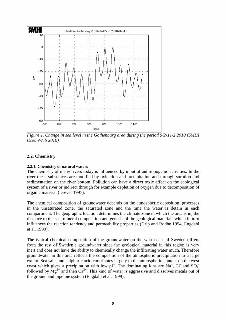
(Sjöfartsverket 2010). Figure 1 gives an example of the daily variation in sea level in the
Gothenburg area.
8
Figure 1. Change in sea level in the Gothenburg area during the period 5/2-11/2 2010 (SMHI
OceanWeb 2010).
2.2. Chemistry
2.2.1. Chemistry of natural waters
The chemistry of many rivers today is influenced by input of anthropogenic activities. In the
river these substances are modified by oxidation and precipitation and through sorption and
sedimentation on the river bottom. Pollution can have a direct toxic affect on the ecological
system of a river or indirect through for example depletion of oxygen due to decomposition of
organic material (Drever 1997).
The chemical composition of groundwater depends on the atmospheric deposition, processes
in the unsaturated zone, the saturated zone and the time the water is detain in each
compartment. The geographic location determines the climate zone in which the area is in, the
distance to the sea, mineral composition and genesis of the geological materials which in turn
influences the reaction tendency and permeability properties (Grip and Rodhe 1994, Engdahl
et al. 1999).
The typical chemical composition of the groundwater on the west coast of Sweden differs
from the rest of Sweden’s groundwater since the geological material in this region is very
inert and does not have the ability to chemically change the infiltrating water much. Therefore
groundwater in this area reflects the composition of the atmospheric precipitation to a large
extent. Sea salts and sulphuric acid contributes largely to the atmospheric content on the west
coast which gives a precipitation with low pH. The dominating ions are Na+, Cl
- and SO4
-
followed by Mg2+
and then Ca2+
. This kind of water is aggressive and dissolves metals out of
the ground and pipeline system (Engdahl et al. 1999).
9
2.2.2. Chemical reactions
When water comes into contact with solids equilibrium is strived to be reached between the
elements in the different mediums. Several reactions and processes are involved in this strive
for equilibrium e.g. oxidation and reduction reactions (redox), sorption (adsorption,
absorption, desorption and ion-exchange), dissolution reaction of solids and gas which are
dependent or independent of pH and mass transport processes of solutes (diffusion, advection,
dispersion). These processes determine the chemical composition of the groundwater and the
nature of the aquifer (Fetter 1994, Drewer 1997, Hitchon et al. 1999).
Since aquifer properties vary greatly with location and the surrounding environment it is hard
to set general values of parameters controlling the main processes determining the
groundwater’s composition. For examples redox condition can be indicated by a systems pE
value. Redox conditions control which species are dissolved in a solution and which
precipitate and is influenced by oxygen concentration and the dominating redox-pair. A
natural system is comprised of many species that are part of several different redox-pairs and
an equilibrium is almost never reached (Drewer 1997, vanLoon and Duffy 2005). According
to Drewer (1997) it is better to think of pE as ―high‖ or ―low‖ for a system without specifying
a number.
Depending on the aquifer properties different reactions control the redox condition.
In rivers, lakes and the sea the redox conditions are largely controlled by plant
photosynthesis:
CO2 + sunlight Corganic + O2, (2)
and bacterial decomposition of organic material.
As long as oxygen respiration occurs, which is the reverse of the photosynthesis reaction (2),
CO2 is released into the water environment, which leads to a decrease in pH. When there is no
O2 left, the decay of organic matter continues by other oxidizing reactions (where micro
organisms often are involved as catalysts) with successively lower pE levels as the
dominating redox-pair changes (Fetter 1999, Drever 1997).
For shallow aquifers with short residence time free oxygen is present and the pE-value is
above 10 and controlled by the O2-H2O redox-pair. Many groundwaters are controlled by the
Mn2+
-MnO2 and Fe2+
-Fe(OH)3 redox pairs and have pE values ranging from -2 to 14 (and no
oxygen present). pE values of -6 to 0 (buffered by the SO42—
H2S redox-pair) are common for
aquifers with long residence time and high content of reactive organic material (high content
of organic material drives down the pE) (Drever 1997).
Anoxic groundwater will be oxygenised when it flows out into surface water. If the
groundwater contains high concentrations of dissolved iron (Fe2+
) this can be shown by the
precipitation of hydroxides at the groundwater/surface water interface and sometimes
aluminium and manganese compounds also precipitate (Knutsson and Morfeldt 2002).
2.2.3. Mass transport of solutes
Apart from the chemical reactions controlling which elements that are in solution and which
are precipitated, mass transport of the solutes also influence the composition of the
groundwater. Advection, diffusion, dispersion, chemical and physical retardation are some of
the processes describing mass transport in a porous material.
10
Advection is the transportation of substances through the flowing groundwater in a porous
material and can be explained with the average linear velocity (vx) described by Darcy’s law:
dx
dh
n
Kv
e
x (3)
vx= average linear velocity
K= hydraulic conductivity
dh/dx= hydraulic gradient
ne= effective porosity
Diffusion is the process where dissolved molecular and ionic species move from areas with
higher concentrations to areas with lower concentrations. Under steady state situation
diffusion is described by Fick’s first law and in systems with changing concentrations Fick’s
second law can be applied (one dimensional systems). Diffusion is faster in pure water than in
porous material where it only can take place in open pores and this is accounted for by using a
diffusion constant representing the porosity (Fetter 1994).
Dispersion is a process that dilutes the solute and lowers the concentration of constituents in
the groundwater. There is both hydrodynamic and mechanical dispersion. Mechanical
dispersion arises with flow through a pore. Molecules in the middle will travel faster than
others because of lower friction and a splitting effect occurs of the flow path which branches
out to the sides. The longitudinal dispersion is greater than the lateral dispersion so solute will
spread in the direction of groundwater movement more than in the direction perpendicular.
Hydrodynamic dispersion includes both molecular diffusion and mechanical dispersivity since
they can not be separated in flowing groundwater (Fetter 1994).
By combining advection, diffusion and dispersion processes into an equation, the
concentration at some distance from a constant source of contamination with a certain
concentration at a certain time can be calculated (Fetter 1994).
Retardation of a solute transport can be chemical, biochemical and physical and results in a
slower transport than what the advection indicates. One retardation process is adsorption of
ions on mineral surfaces due to electrical charges. Clays are good adsorbers because of their
large specific surface (m2/g dry soil) and often high electrical charge. Anthropogenic organic
compounds can be adsorbed by organic material in the soil. Organic compounds solubility
control how mobile they are in the environment and it can be revealed by their octanol-water
partition coefficient (Koc) which determines the distribution of the compound in a certain soil
(Fetter 1994). Micro organisms that brake down organic compounds to obtain energy from the
carbon atom will also retard the spreading of organic pollutants to different extent depending
on species and concentration. Biodegradation processes are used as a remediation technique;
bioremediation (Drever 1997).
2.3 Urban hydrogeology
2.3.1. Urban surfaces, constructions and material
The hydrogeology of an urban environment is affected by a city’s constructions and is very
different and complex from a natural environment. A city has extensive hard surfaces which
are impermeable for water and for example affects the groundwater recharge due to increase
11
of surface runoff which is one of the factors controlling the groundwater level. Other factors
affecting the urban hydrogeology are, e.g. leaking water pipes and sewers, which either
contribute to groundwater recharge or drain groundwater from the geological strata lowering
or rising the groundwater table; city climate, controlling the amount of water initially reaching
the ground; and runoff, in form of storm water. Since every city is different in geologic
setting, infra structure and climate, Norin (2004) states that a generalisation of the overall
affect on hydrogeology due to urbanisation of cities, is not possible.
However, a generalisation of different parts of the urban system can be made to simplify an
overall description. Classifying different parts such as urban surfaces after so-called
―Functional Facies‖ is a way to describe its characteristics and how it influences water and
sediment transport including the pollution carried with them. Different properties and
characteristics such as permeable, hard and green area surfaces can be given classification
substantives like B for brown permeable surface, H for hard impermeable surface and G for
green vegetated surface respectively. Adjectives describing the different surface classes can
be added to the substantives related for instance to probable pollution sources (e.g. heavy
traffic, or leachates from metal sources and asphalt depository stacks) and drainage and runoff
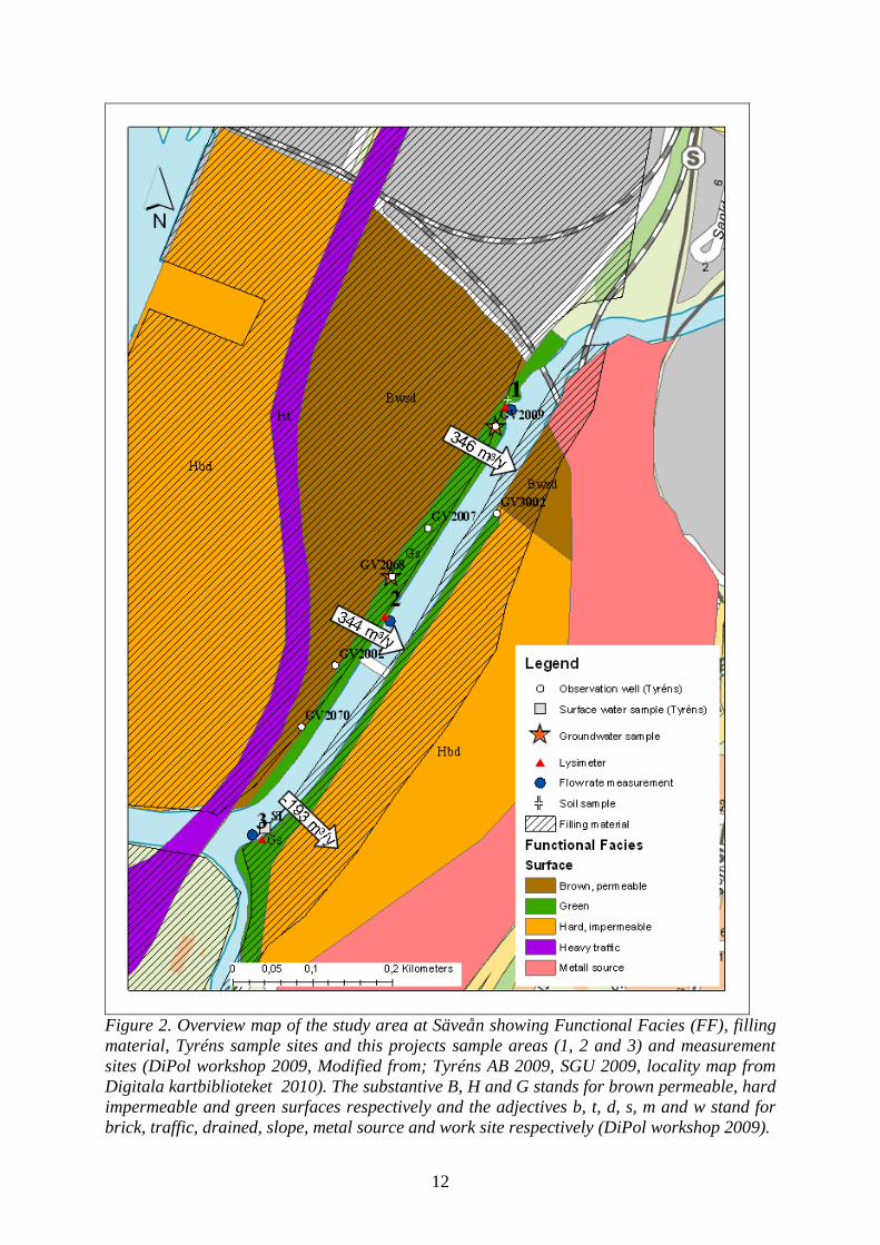
properties. This type of mapping was done at the DiPol workshop 2009 (Figure 2, DiPol
workshop 2009).
12
Figure 2. Overview map of the study area at Säveån showing Functional Facies (FF), filling
material, Tyréns sample sites and this projects sample areas (1, 2 and 3) and measurement
sites (DiPol workshop 2009, Modified from; Tyréns AB 2009, SGU 2009, locality map from
Digitala kartbiblioteket 2010). The substantive B, H and G stands for brown permeable, hard
impermeable and green surfaces respectively and the adjectives b, t, d, s, m and w stand for
brick, traffic, drained, slope, metal source and work site respectively (DiPol workshop 2009).
13
Previous attempts of grouping different urban geologic settings have been done by for
example Hultén (1997), where among other things the relation between groundwater levels in
Gothenburg and the urban environmental influence were studied. Four types of settings were
used to classify the measurements of groundwater levels in Gothenburg (Hultén 1997). The
ground surface around observation wells used in Hulténs study were also mapped in five
classes; impermeable ground (buildings), impermeable ground (asphalt), cobblestone or
gravel, water and green area, (similar to those used in the DiPol workshop 2009 but not linked
to pollution sources in the same way) to give an understanding of the infiltration capacity and
the groundwater levels response to precipitation (Hultén 1997).
2.3.2. Urban groundwater quality
The rain water passes several sources of elements along its pathway that influence its
composition. Already in the atmosphere pollution sources due to anthropogenic activities such
as vehicle exhausts are introduced together with dust particles from buildings, roads, sea
water and geologic formations (van Loon and Duffy 2005). Reaching the urban ground
surface, often a hard impermeable surface like roofs of buildings or paved areas, substances
derived from the activity of a city influences the water chemistry. How much the water is
influenced before it continues its travel depends on the initial chemistry of the water hitting
the surface, the intensity of the precipitation, the ground surfaces properties and the time spent
on the surface, which is controlled by surface slope and the handling of runoff water through
channel and drainage systems. Urban runoff can take several ways when leaving the ground
surface: 1) it can leave the surface as storm water straight into surface waters, 2) it can enter
the sewer and runoff system trough drainage wells leading to treatment plants, and 3) it can
infiltrate permeable urban surfaces reaching the unsaturated zone getting further influenced by
underground constructions and geological material. Leakage from sewers, storm sewers,
water mains, septic tanks, underground buildings, filling material and storage tanks contribute
to the pollution of groundwater. The infiltrated water can also influence the soil it enters by
depositing pollutants carried with it, due to changed chemical and physical conditions (Norin
2004).
2.3.4. PAHs in the environment
PAHs (Polycyclic aromatic hydrocarbons) are produced during any type of combustion,
natural in smaller extent and anthropogenic to larger extent, and are therefore present
everywhere in our environment (Naturvårdsverket 2010, Kemikalieinspectionen 2010).
Hydrocarbons can be divided into two classes: aromatic hydrocarbons containing benzene
rings and aliphatic hydrocarbons which do not contain benzene rings. Polycyclic aromatic
hydrocarbons (PAH) consist of two to eight benzene rings joined together and are found in
e.g. high aromatic oils, coal tar and creosote. PAH also form through incomplete combustion
of fossil fuels (Fetter 1999, van Loon and Duffy 2005, Kemikalieinspectionen 2010).
Properties such as melting and boiling points, specific gravity, water solubility, octanol-water
partition coefficient, vapour pressure and vapour density of an organic compound govern its
movement in the environment. The boiling point of hydrocarbons is correlated to the number
of carbon atoms in the species. The ligthest/smallest species are volatile while the
heavier/larger are present as solids usually as surface deposits on combustion particles such as
soot (van Loon and Duffy 2005). When petroleum is separated into different fractions by
distillation, species with similar numbers of carbon atoms end up together (Fetter 1999).
In this work the PAH species in Table 1 were analysed (the IVL laboratory).
14
Table 1. Analysed PAHs in this project and number of benzene rings (IVL laboratory).
PAH species (IVL)
Number of benzene rings
(Fetter 1999).
Naphthalene 2
Acenaphthene 2
Flourene 2
Phenanthrene 3
Anthracene 3
Flouranthene 3
Pyrene 4
Benzo(a)anthracene 4
Chrysene 4
Benzo(b)flouranthene 4
Benzo(k)flouranthene 4
Benzo(a)pyrene 5
Dibenz(a,h)anthracene 5
Benzo(g,h,i)perylene 6
Indeno(1,2,3-cd)pyrene 5
Among PAHs several of the most active carcinogenic species known are found: 7,12-
dimethylbenzo(a)anthracene, 3-methylcolantrene, dibenzo(a,h)anthracene, dibenzo(a)pyrene,
dibenzo(a,h)pyrene and dibenzo(a,i)pyrene. Among the moderate active are:
Benzo(a)anthracene and Benzo(e)pyrene. All these compounds give rise to skin cancer if
applied on skin, inhalation has shown to give lung cancer and laboratory tests on animals have
shown that injection gives rise to liver tumours (Birgerson et al. 2009).
From about 1850-1950 gas for residential and commercial use was produced by heating coal
in absence of oxygen separating volatile fractions from the coal leaving pure carbon (known
as coke). By cooling gas from a coal gas manufacturing plant, liquid hydrocarbons separate
out as oils and tars, these can be further refined into valuable chemicals e.g. benzene (found in
gasoline), toluene (found in gasoline), aspirin (used in the pharmaceutical industry) and
creosote (used for preservation of wood). Carburetted water gas process is another way of
manufacturing tar (Fetter 1999). Contamination of soil and groundwater is a result of the use
and release of these products. Gasoline and diesel contamination are linked to e.g. leaking
underground storage, refineries, pipelines and terminals. Contaminants from coal and
carburetted water gas plants can be found at old manufactured gas plants, byproduct coke
oven locations and tar refinery sites (Fetter 1999).
The solubility of hydrocarbons varies significantly and they are therefore found to different
extent in gasoline, diesel fuel, coal tar and carburetted water gas tar. PAHs have low solubility
in water and will be present there in very small amounts but in the contrary be present in
higher concentrations in soils. Old coal tar sites often have high content in PAHs.
Hydrocarbons can to different extent undergo biological degradation (Fetter 1999).
15
PAH compounds have been identified in regions remote from major sources of combustion
e.g. a concentration of 1 ng/m3 was found in air measurements in the Artic regions of North
America. In comparison air measurements in the industrial city Hamilton, Ontario, indicated
about 10 ng/m3 PAH in the summer and 30 ng/m
3 in the winter. The finding of PAH in
remote areas show that they have a non-reactive nature while travelling in the air (van Loon
and Duffy 2005). Vehicle exhaust, tyre ware and road ware are the major sources of PAH to
the atmosphere in larger cities. A big part of the PAH spread in the atmosphere finally reaches
water environments where they accumulate in sediments (Kemikalieinspectionen 2010).
3. The study area
3.1. Site description
3.1.1. Site location
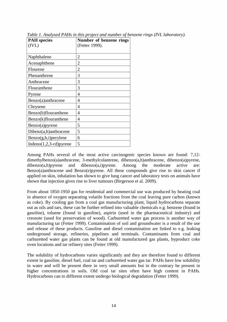
The study site is located in urbanised parts of the Säveån stream which is situated in
Gothenburg on the west coast of Sweden (Figure 3). Säveån belongs to the Göta älv River
drainage area and is located in the administration water district of Västerhavet (Lång et al.
2005). Säveån has a drainage area of about 1500 km2 and an average annual discharge of 18
m3/s. It has its source in Lake Anten and Lake Säven north of the town Borås and flows via
Lake Mjörn through the valley Sävedalen to Sävelången and then further through Lake Aspen
down to its outlet in the bigger river Göta älv. Göta älv flows from Lake Värnern in the north
to the sea area Kattegatt in the south outside Gothenburg. North of Gothenburg, at Kungälv,
the river divides into two branches: a north branch named Nodre älv and a south branch
keeping the name Göta älv (Göta älvs vattenvårdsförbund 2005).
River
County
Lake
Forest
Urban area
Catchment area
Study area
Legend
Goth
enburg
Säveån
N
Figure 3. Overview map of the Säveån Stream showing the location of the study area (red
circle) in this project (Länsstyrelsernas GIS tjänster 2010).
16
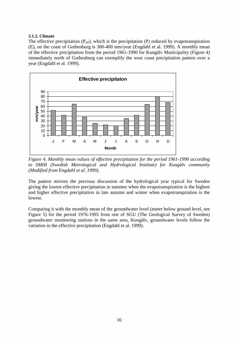
3.1.2. Climate
The effective precipitation (Peff), which is the precipitation (P) reduced by evapotranspiration
(E), on the coast of Gothenburg is 300-400 mm/year (Engdahl et al. 1999). A monthly mean
of the effective precipitation from the period 1961-1990 for Kungälv Municipality (Figure 4)
immediately north of Gothenburg can exemplify the west coast precipitation pattern over a
year (Engdahl et al. 1999).
Effective precipitaton
0
10
20
30
40
50
60
70
80
90
J F M A M J J A S O N D
Month
mm
/year
Figure 4. Monthly mean values of effective precipitation for the period 1961-1990 according
to SMHI (Swedish Metrological and Hydrological Institute) for Kungälv community
(Modified from Engdahl et al. 1999).
The pattern mirrors the previous discussion of the hydrological year typical for Sweden
giving the lowest effective precipitation in summer when the evapotranspiration is the highest
and higher effective precipitation in late autumn and winter when evapotranspiration is the
lowest.
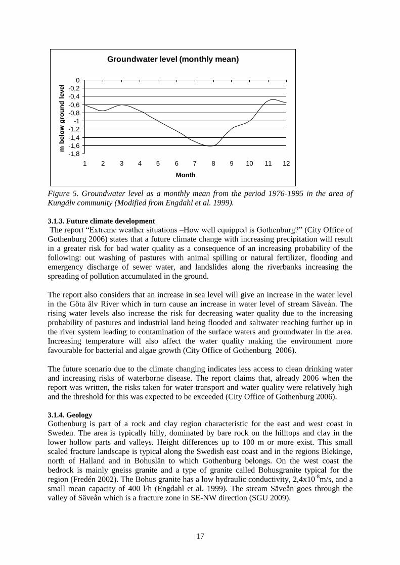
Comparing it with the monthly mean of the groundwater level (meter below ground level, see
Figure 5) for the period 1976-1995 from one of SGU (The Geological Survey of Sweden)
groundwater monitoring stations in the same area, Kungälv, groundwater levels follow the
variation in the effective precipitation (Engdahl et al. 1999).
17
Groundwater level (monthly mean)
-1,8
-1,6
-1,4
-1,2
-1
-0,8
-0,6
-0,4
-0,2
0
1 2 3 4 5 6 7 8 9 10 11 12
Month
m b
elo
w g
rou
nd
level
Figure 5. Groundwater level as a monthly mean from the period 1976-1995 in the area of
Kungälv community (Modified from Engdahl et al. 1999).
3.1.3. Future climate development
The report ―Extreme weather situations –How well equipped is Gothenburg?‖ (City Office of
Gothenburg 2006) states that a future climate change with increasing precipitation will result
in a greater risk for bad water quality as a consequence of an increasing probability of the
following: out washing of pastures with animal spilling or natural fertilizer, flooding and
emergency discharge of sewer water, and landslides along the riverbanks increasing the
spreading of pollution accumulated in the ground.
The report also considers that an increase in sea level will give an increase in the water level
in the Göta älv River which in turn cause an increase in water level of stream Säveån. The
rising water levels also increase the risk for decreasing water quality due to the increasing
probability of pastures and industrial land being flooded and saltwater reaching further up in
the river system leading to contamination of the surface waters and groundwater in the area.
Increasing temperature will also affect the water quality making the environment more
favourable for bacterial and algae growth (City Office of Gothenburg 2006).
The future scenario due to the climate changing indicates less access to clean drinking water
and increasing risks of waterborne disease. The report claims that, already 2006 when the
report was written, the risks taken for water transport and water quality were relatively high
and the threshold for this was expected to be exceeded (City Office of Gothenburg 2006).
3.1.4. Geology
Gothenburg is part of a rock and clay region characteristic for the east and west coast in
Sweden. The area is typically hilly, dominated by bare rock on the hilltops and clay in the
lower hollow parts and valleys. Height differences up to 100 m or more exist. This small
scaled fracture landscape is typical along the Swedish east coast and in the regions Blekinge,
north of Halland and in Bohuslän to which Gothenburg belongs. On the west coast the
bedrock is mainly gneiss granite and a type of granite called Bohusgranite typical for the
region (Fredén 2002). The Bohus granite has a low hydraulic conductivity, 2,4x10⁻⁸
m/s, and a
small mean capacity of 400 l/h (Engdahl et al. 1999). The stream Säveån goes through the
valley of Säveån which is a fracture zone in SE-NW direction (SGU 2009).
18
The typical stratigraphy in Gothenburg is typified by lowermost coarse grained sediment,
often containing more glaciofluvial than till sediments, overlain by younger fine grained
sediments, first (stratigraphically lower) glacial clay and, in lower terrain areas, postglacial
clay (Magnusson 1978, Fréden 2002). The clays on the west coast are typical stiff, dark grey
in colour with poor lamination and have often a high risk for quick-clay land slides (Stevens
et al. 1990, Fredén 2002).
The typical Gothenburg stratigraphy has been shown during several building projects in the
area. For example in the district Gamlestaden located in the project area of this work, a
drilling document from 1969 (of Bo Alte AB) shows 13 m of cohesive material overlaying 57
m of frictional material. According to Adrielsson and Fredén (1987) the frictional material
can be interpreted to consist fully or mostly of glaciofluvial deposits. Another example is at
Sävenäs, located on the south side of Säveåns valley, where gravel has been encountered
under clay (Magnusson 1978).
Glaciofluvial deposits are found more or less in Gothenburg with surroundings but are more
common in the fracture valley systems. Säveån has less glaciofluvial deposits than the other
valleys in the area (e.g. the valley parallel to Säveåns valley with the well defined delta;
Skallsjödeltat) and little is visible at the surface (Magnusson 1978).
The till layer in Gothenburg is thin but has in some places accumulated in thicker formations
forming stoss and lee moraines (e.g. Dösebackamoränen) or ice-marginal moraines (Fréden
2002). Göteborgsmoränen is an ice-marginal moraine which is found from the Halland region
to north of Gothenburg. It is a complex moraine form containing deltas and ridges composed
of sand and gravel, till and lenses of finer sediment (SGU 1998, Fréden 2002).
In a hydrogeologic perspective Säveån valley is described to consist of thick continuous fine
grained sediment layers, mainly glacial clay, where lentils of water conducting sand and
gravel can occur in and under it. Some areas with groundwater supply can exist in sand and
gravel layers or in loose till overlain by sealed or poorly permeable sediment layers (SGU
1998).
3.1.5. Filling material
Except the natural stratigraphy described earlier there is an anthropogenic upper layer of
filling material in the central parts of Gothenburg as in many other cities. Hultén (1997) has
made a compilation of existing sources of information about filling material in Gothenburg
and made a general picture of its composition. The upper 1-2 m consist of some form of road
body or drainage systems around buildings usually composed of macadam, sand and/or
gravel. The next 1-2 m beneath consists of loose filling composed mostly of the quaternary
deposits of the region, for Gothenburg it is clay and spilling material like wood, glass and
bricks. The upper layer in a city is relatively comparable to other cities because many
technical regulations and construction norms are similar (Hultén 1997).
In some parts of Gothenburg extensive filling work has been done, mainly around the Göta
älv River. The filling thickness in the areas Gullbergsvass, the railroad tracks and areas
adjacent to the river has a mean of 3 m (Hultén 1997). The thickness of the filling material in
the area of this project is assumed to lie around 3 m as well since the groundwater wells
(Figure 2) used, reach only the filling material and have a maximum depth of 3 m
(Cliffordson L. pers.comm 2009)
19
3.1.6. The aquifer system
There are two main aquifers in Gothenburg, one lower confined aquifer under the clay layer
which consists of till and glaciofluvial deposits and one unconfined aquifer which lies mainly
in the filling material spread out in the central parts of Gothenburg (Hultén 1997). The aquifer
system in the project area is assumed to have this stratigraphy structure as well. The
groundwater mean temperature in Gothenburg is between 7-7,5 ºC and gets gradually warmer
towards the coast (Engdahl et al. 1999).
3.2. Industrial history of Säveån
Säveåns valley has a long industrial history which started in the 18th
century with big
expansions during the 19th
and the 20th
century continuing into the 21th
century. The activities
conducted in the area range from small water mills to big industrial sites in the city of
Gothenburg. Water power plants and train communications have been important for the
development of the city. Fishing and agricultural activities are also important to point out in
the development of Säveåns valley. The industries are concentrated relative far downstream
Säveån, naturally explained by the near distance to Gothenburg and the railroad tracks.
Textile industry and ironworks are two early industries that established along Säveån. In
Gothenburg central parts, the brothers Sahlgren sugar factory (1720´s) at Gamlestaden was
followed by Gamlestadens factory, SKF (The Swedish ball-bearing factory) and other
activities. SKF together with Renovas waste heating power plant are the biggest facilities
from late 1900 in the area. The exploration pressure is high in these downstream parts of
Säveån (von Arbin et al. 2008).
3.3. Pollution and water treatment at the study site
3.3.1. Project “Partihallförbindelsen”
In the work plan for the road junction project ―Partihallsförbindelsen‖ in Gothenburg the EIA
(Environmental Impact Assessment, MKB in Swedish) documents the contaminant situation
of the site at Partihallarna (year 2004), when the EIA was completed (Samuelsson 2004).
The ongoing road building at the site for this thesis work consists of a long bridge that goes
over the area Partihallarna, crossing several railway roads and the stream Säveån, and is part
of a the bigger road project ―Marieholmsförbindelsen‖ connecting the E6, E45 and E20 roads
(Figure 6). The bridge will connect the E20 road east of Säveån with the E45 road and two
bridge ramps leading to a new tunnel under the Göta älv River on the west side of the stream
Säveån. The intention of the Marieholmförbindelsen project is to decrease the heavy traffic on
the E6 road through the Tingstad tunnel and at the road junctions
Olskroksmotet/Gullbergsmotet.
20
E45
Levels above MKM
Ground pollution
Levels above
acceptance criteria
E45
Levels above MKM
Ground pollution
Levels above
acceptance criteria
Levels above MKM
Ground pollution
Levels above
acceptance criteria
Levels above MKM
Ground pollution
Levels above
acceptance criteria
Partih
alla
rnaM
arieholm
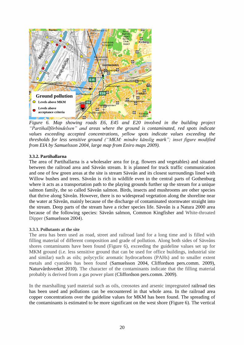
Figure 6. Map showing roads E6, E45 and E20 involved in the building project
“Partihallförbindelsen” and areas where the ground is contaminated, red spots indicate
values exceeding accepted concentrations, yellow spots indicate values exceeding the
thresholds for less sensitive ground (“MKM: mindre känslig mark”; inset figure modified
from EIA by Samuelsson 2004, large map from Eniro maps 2009).
3.3.2. Partihallarna
The area of Partihallarna is a wholesaler area for (e.g. flowers and vegetables) and situated
between the railroad area and Säveån stream. It is planned for truck traffic communication
and one of few green areas at the site is stream Säveån and its closest surroundings lined with
Willow bushes and trees. Säveån is rich in wildlife even in the central parts of Gothenburg
where it acts as a transportation path to the playing grounds further up the stream for a unique
salmon family, the so called Säveån salmon. Birds, insects and mushrooms are other species
that thrive along Säveån. However, there is no widespread vegetation along the shoreline near
the water at Säveån, mainly because of the discharge of contaminated stormwater straight into
the stream. Deep parts of the stream have a richer species life. Säveån is a Natura 2000 area
because of the following species: Säveån salmon, Common Kingfisher and White-throated
Dipper (Samuelsson 2004).
3.3.3. Pollutants at the site
The area has been used as road, street and railroad land for a long time and is filled with
filling material of different composition and grade of pollution. Along both sides of Säveåns
shores contaminants have been found (Figure 6), exceeding the guideline values set up for
MKM ground (i.e. less sensitive ground that can be used for office buildings, industrial site
and similar) such as oils; polycyclic aromatic hydrocarbons (PAHs) and to smaller extent
metals and cyanides has been found (Samuelsson 2004, Cliffordson pers.comm. 2009),
Naturvårdsverket 2010). The character of the contaminants indicate that the filling material
probably is derived from a gas power plant (Cliffordson pers.comm. 2009).
In the marshalling yard material such as oils, creosotes and arsenic impregnated railroad ties
has been used and pollutions can be encountered in that whole area. In the railroad area
copper concentrations over the guideline values for MKM has been found. The spreading of
the contaminants is estimated to be more significant on the west shore (Figure 6). The vertical
21
spreading is relative wide and reaches down to the old stream bottom approximately 4 meters
(Samuelsson 2004).
During the building of the new bridge large areas of the contaminated ground will be
involved, especially along the west shoreline. It is not decided how and how much of the
contaminated masses will be treated. The EIA states that masses will be handled so that the
surrounding does not get harmed. Some of the ground along the east shore will be involved
during the building of the bridge pillars, these masses will be cleaned. Other contaminated
masses that are removed will be taken to a local depository. Some of the ground material at
Säveån has contaminant concentrations so high it has to be stored at a class 1 depository, for
example at the SAKAB treatment facility (Samuelsson 2004, SAKAB homepage 2010).
Measurements show that Säveåns water is turbid and well oxygenated and shows no
acidification but the bacteria content and concentration of metals increase towards the outlet
into the Göta älv River (Samuelsson 2004).
The environmental management (Miljöförvaltningen) has studied environmental hazardous
activities along Säveåns drainage area. They found that out of 500 different activities, about
15 needed stricter environmental requirements at the time when the investigation was done.
The ground around some of these activities is contaminated, but how it affects Säveån is hard
to determinate according to the environmental management (Samuelsson 2004).
3.3.4. Treatment of stormwater at the site
Stormwater from the south part of the road junction Mariholmsmotet goes through a
combined pump station at the bridge Kodammsbron in the area and then further to a treatment
plant. Under intense rainstorms the combined system can be flooded and water can go directly
to the recipient, the stream Säveån. Stormwater from the area between Säveån and the road
E20 goes into the municipal drainage system for stormwater which leads directly into Säveån
without treatment. The E20 road has a separate system, leading stormwater direct into Säveån
(Samuelsson 2004).
Sedimentation basins will be built on both the west and east sides of Säveån for treatment of
runoff water coming from the new bridge before it is discharged into the Göta älv River and
the stream Säveån, respectively. This will improve the condition of water led into Säveån
compared to the situation before the project. The new road will however contribute with more
contaminants to the runoff water due to increased car traffic in the area, but it will be treated
at sedimentation facilities before it is let out into Säveån. Significant changes for the
ecological system in the Säveån stream are not expected since large volumes of polluted water
still reach the stream at other locations (Samuelsson 2004).
The water society of Göta älv River (Göta älvs vattenvårdsförbund) has analysed the water at
the outlet of Säveån for acidity, copper, zinc and oxygen consuming species. They land under
the set norm value of MKN (miljökvalitetsnormen), which is a juridical means of control
regulated in the Environmental Code (Miljöbalken). The oxygen concentration is 11 mg/l
which exceeds the lowest MKN norm 9 mg/l set for oxygen and therefore is approved
(Samuelsson 2004).
22
3.4. Previous and ongoing work
3.4.1. Göta älvs vattenvårdsförbund
Today (2010) ‖Göta älvs vattenvårdsförbund‖, The water society of Göta älv River, takes
continuous samples at seven fixed computerised stations along the Göta älv River. The system
gives out a warning alarm if the water quality is changed and the intake of water to the
drinking water supply needs to be closed. The control program also includes some 60
tributaries to Göta älv, where Säveån is one of them (Göta älvs vattenvårdsförbund 2010).
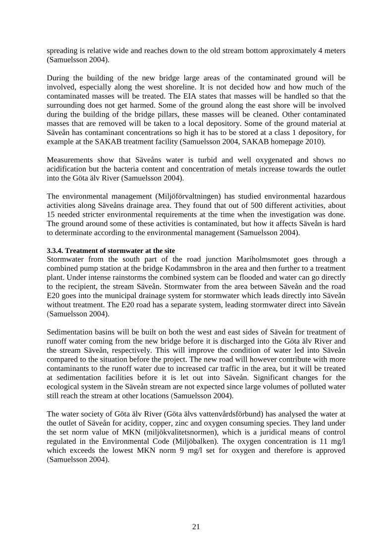
The report from 2008 control program covers 16 sample sites along Säveån, one is situated in
the study area of this work. The report gives information of calculated values of the annual
average recharge for 2008 and for the period 1981-2008 (Figure 7), calculated material
transport for nitrogen and phosphor and its development trough 2006-2008. The results from
the analysis of the 16 sample sites are presented and the condition classed after The Swedish
Environmental Protection Agancy (Naturvårdsverkets) standards/norms from 1999, based on
a mean value from the period 2006-2008 (Göta älvs vattenvårdsförbund 2008).
Discharge at Jonsered, Säveån, monthly mean (m3/s)
010203040506070
Jan
Feb
Mar
Apr
Maj
Jun
Jul
Aug
Sep
Okt
Nov
Dec
mean(y
ear)
month
dis
ch
arg
e (
m3/s
)
1981-2008
2008
Figure 7. Diagram showing the discharge (m
3/s) in Säveån at Jonsered, adjacent to
Gothenburg, as monthly mean for year 2008 and the period 2006-2008) (data from Göta älvs
vattenvårdsförbund 2008) 3.4.2. The Säveån project
The County Administrative Board of Västra Götalands län (Länstyrelsen) and Västarvet
(―West Heritage‖) has started a project called Säveånprojektet (2006) with the aim to keep a
long-term sustainable development of Säveåns valley. The interests lie in both cultural and
nature values mainly related to the water environment and the use of it, but also in landscape
and the history of industries (Västarvet 2010, Västra Götalands län 2010).
3.4.3. Tyréns AB
Before and during the project of building Partihallsförbindelsen Tyréns, one of Sweden’s
leading consulting companies, is in charge of investigating the groundwater and surface water
along Säveån (Figure 2). The sampling of water is to be done four times every year and the
purpose is to improve the knowledge of the area concerned and assure no unacceptable
leakage of pollutants occurs during the building. Sampling has been done since September-
November 2008 and earlier two times by another consulting company WSP (Tyréns AB
2009).
23
3.4.4. The Natura 2000-network
Valuable nature in EU is gathered in a Natura 2000-network to protect and preserve flora and
wildlife for future generations. The Natura 2000-network was created to protect endangered
species and prevent the destroying of their habitats. In Sweden the Swedish environmental
protection agency (Naturvårdsverket) is in charge of the protection work but The County
Administrative Board (Länstyrelsen) does most of the practical work together with the
forestry board, municipalities, fishers, landowners and other (Naturvårdsverket 2010). Parts of
stream Säveån are within a Natura 2000 area, including the part studied in this work.
4. Methods
4.1. Field work planning
4.1.1. Sample areas
Available chemical analyses from existing observation wells in the study area were compiled
(Tyréns 2009). Based on the information relevant for the specific project area of the DiPol
workshop three sites for new measurements were chosen (Figure 2). Two of the available
groundwater observation wells were used, one upstream (GV2009) in Area 1 and one more
downstream (GV2068) in Area 2. The sites for flow rate measurements and other water
samples, including lysimeter samples and outflow samples in Säveån, were chosen within the
areas of interest adjacent to the groundwater wells (Figure 2). The field work was carried out
in November 2009 and involved flow rate measurements and sampling of groundwater and
soil.
4.2. Field work
4.2.1. Flow rate measurements
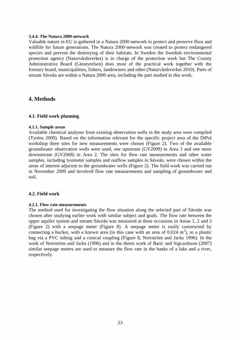
The method used for investigating the flow situation along the selected part of Säveån was
chosen after studying earlier work with similar subject and goals. The flow rate between the
upper aquifer system and stream Säveån was measured at three occasions in Areas 1, 2 and 3
(Figure 2) with a seepage meter (Figure 8). A seepage meter is easily constructed by
connecting a bucket, with a known area (in this case with an area of 0,024 m2), to a plastic
bag via a PVC tubing and a conical coupling (Figure 8, Norrström and Jacks 1996). In the
work of Norrström and Jacks (1996) and in the thesis work of Baric and Sigvardsson (2007)
similar seepage meters are used to measure the flow rate in the banks of a lake and a river,
respectively.
24
Stream bank
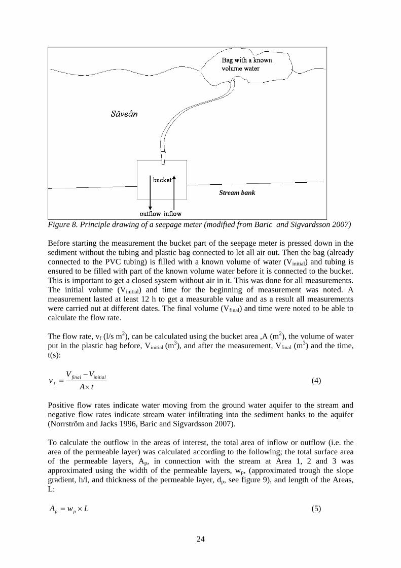
Figure 8. Principle drawing of a seepage meter (modified from Baric and Sigvardsson 2007)
Before starting the measurement the bucket part of the seepage meter is pressed down in the
sediment without the tubing and plastic bag connected to let all air out. Then the bag (already
connected to the PVC tubing) is filled with a known volume of water (Vinitial) and tubing is
ensured to be filled with part of the known volume water before it is connected to the bucket.
This is important to get a closed system without air in it. This was done for all measurements.
The initial volume (Vinitial) and time for the beginning of measurement was noted. A
measurement lasted at least 12 h to get a measurable value and as a result all measurements
were carried out at different dates. The final volume (Vfinal) and time were noted to be able to
calculate the flow rate.
The flow rate, vf (l/s m2), can be calculated using the bucket area ,A (m
2), the volume of water
put in the plastic bag before, Vinitial (m3), and after the measurement, Vfinal (m
3) and the time,
t(s):
tA
VVv
initialfinal
f
(4)
Positive flow rates indicate water moving from the ground water aquifer to the stream and
negative flow rates indicate stream water infiltrating into the sediment banks to the aquifer
(Norrström and Jacks 1996, Baric and Sigvardsson 2007).
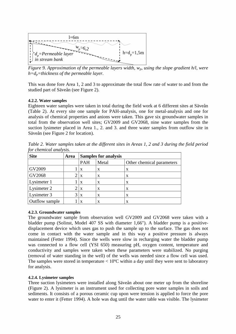
To calculate the outflow in the areas of interest, the total area of inflow or outflow (i.e. the
area of the permeable layer) was calculated according to the following; the total surface area
of the permeable layers, Ap, in connection with the stream at Area 1, 2 and 3 was
approximated using the width of the permeable layers, wp, (approximated trough the slope
gradient, h/l, and thickness of the permeable layer, dp, see figure 9), and length of the Areas,
L:
LwA pp (5)
25
l=6m
h=dp=1,5mdp=Permeable layer
in stream bank
wp≈6,2
Figure 9. Approximation of the permeable layers width, wp, using the slope gradient h/l, were
h=dp=thickness of the permeable layer.
This was done fore Area 1, 2 and 3 to approximate the total flow rate of water to and from the
studied part of Säveån (see Figure 2).
4.2.2. Water samples
Eighteen water samples were taken in total during the field work at 6 different sites at Säveån
(Table 2). At every site one sample for PAH-analysis, one for metal-analysis and one for
analysis of chemical properties and anions were taken. This gave six groundwater samples in
total from the observation well sites; GV2009 and GV2068, nine water samples from the
suction lysimeter placed in Area 1., 2. and 3. and three water samples from outflow site in
Säveån (see Figure 2 for location).
Table 2. Water samples taken at the different sites in Areas 1, 2 and 3 during the field period
for chemical analysis.
Site Area Samples for analysis
PAH Metal Other chemical parameters
GV2009 1 x x x
GV2068 2 x x x
Lysimeter 1 1 x x x
Lysimeter 2 2 x x x
Lysimeter 3 3 x x x
Outflow sample 1 x x x
4.2.3. Groundwater samples
The groundwater sample from observation well GV2009 and GV2068 were taken with a
bladder pump (Solinst, Model 407 SS with diameter 1,66"). A bladder pump is a positive-
displacement device which uses gas to push the sample up to the surface. The gas does not
come in contact with the water sample and in this way a positive pressure is always
maintained (Fetter 1994). Since the wells were slow in recharging water the bladder pump
was connected to a flow cell (YSI 650) measuring pH, oxygen content, temperature and
conductivity and samples were taken when these parameters were stabilized. No purging
(removal of water standing in the well) of the wells was needed since a flow cell was used.
The samples were stored in temperature < 10ºC within a day until they were sent to laboratory
for analysis.
4.2.4. Lysimeter samples
Three suction lysimeters were installed along Säveån about one meter up from the shoreline
(Figure 2). A lysimeter is an instrument used for collecting pore water samples in soils and
sediments. It consists of a porous ceramic cup upon were tension is applied to force the pore
water to enter it (Fetter 1994). A hole was dug until the water table was visible. The lysimeter
26
suction cup was put just under the groundwater table to get samples from the upper most
groundwater (the intersection between water in the saturated zone and the unsaturated zone).
The hole was filled back as undisturbed as possible to try and create the same environment
around it as before the installation. Samples were taken by connecting a suction bottle to the
lysimeter with negative pressure created simply by removing air from the bottle with a hand
pump.
4.2.4. Samples taken from areas of outflow
Where outflow was recognized, through the seepage meter measurements, water samples
were taken for PAH-, metal- and major ion-analysis. This was only done for one site in Area
1. The outflow samples were taken by lowering a bottle, with the cap still on, to just above the
bottom were the seepage meter measurement indicated outflow and then releasing the cap
allowing the bottle to be filled fully before sealed again. It is important to fill the bottle up till
the top and close it while still holding it under water to prevent atmospheric oxygen from
mixing with the sample.
4.2.5. Soil samples
A hole for soil sampling was dug in Area 1 near the lysimeter site and soil samples were taken
in level with the groundwater table. One sample was taken of an oxidized zone; Säveån 1a,
indicated by precipitated oxides, a second sample; Säveån 1c, was taken under the
groundwater table, and a third (Säveån 1b) between the previous two samples (for location
see Figure 2).
A principle sketch over the sites at Area 1 is shown in Figure 11.
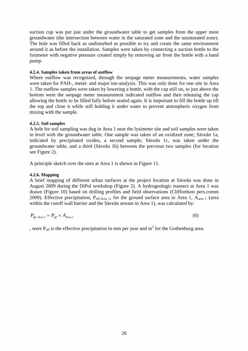
4.2.6. Mapping
A brief mapping of different urban surfaces at the project location at Säveån was done in
August 2009 during the DiPol workshop (Figure 2). A hydrogeologic transect at Area 1 was
drawn (Figure 10) based on drilling profiles and field observations (Cliffordson pers.comm
2009). Effective precipitation, Peff.Area 1, for the ground surface area in Area 1, Aarea 1 (area
within the cutoff wall barrier and the Säveån stream in Area 1), was calculated by:
11. AreaeffAreaeff APP (6)
, were Peff is the effective precipitation in mm per year and m2 for the Gothenburg area.
27
Peff
3300-4400
m3/y
Area 140 m13 m
50 m
?
1,31,1
0,6
0,7
>50 m
GV2009
Barrier, reaches
down to clay
3
2
2,5
> 2 > 2
2
> 3
3 m
?
20
10
20
18
? 20
54
20
55
Säveån
average
annual
discharge
18 m3/s
0,69
10 m
346 m3/y ?
1,2
Water surfacePermeable
Imp
erm
eab
le, d
rain
ed
Partly permeable
sloping
Pa
rtly
perm
eab
le
Steep
slop
e
Impermeable,
drained
shaft
Area 1
Permeable layers
about 1,5 m
W EThe water budget figures are calculated
for the whole surface area in Area 1
Old wharf construction
Drainage system
Silty mud (siGy)
Mud and clay (leGy, gyLe)
Sandy silt containing some mud (gysaSi, saSi)
Silty sandy mud (siSaGy) , (black)
Asphalt (impermeable)
Brown surface (permeable)
Green surface
Drilling profile22
Groundwater table
Water flow
Fill material (coubble, gravel, sand and brick material)
Water budget (m3/y)
Figure 10. Transect at Area 1 showing a principle sketch of the stratigraphy profile stretching
from about 100 m up from the west shoreline at Marieholm through Säveån to about 50 m up
on the east shoreline at Partihallarna. Functional Facies surfaces, hydrological barriers and
approximated water flow and water budget (shown by the arrows) are included where Peff is
the effective precipitation (Borehole documents, pers. comm. Cliffordson Vägverket 2009).
4.3. Laboratory work
4.3.1. Water samples
The water samples for PAH analysis were sent to the IVL (The Swedish Environmental
Research Institute) laboratory, the water samples for metal and other chemical analysis were
28
sent to the ALS Scandinavia AB laboratory and the soil samples were analysed in the
laboratory at the Department of Earth science, University of Gothenburg.
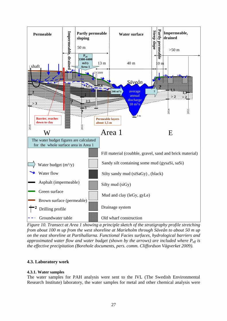
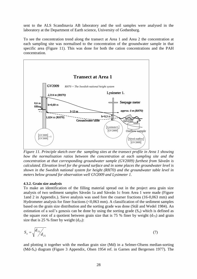
To see the concentration trend along the transect at Area 1 and Area 2 the concentration at
each sampling site was normalised to the concentration of the groundwater sample in that
specific area (Figure 11). This was done for both the cation concentrations and the PAH
concentration.
GV2009
Lysimeter 1.
Seepage meter
l=13 m
h=0,69 m
Groundwater table
h=0,3 m
2,314 m (RH70)
approx. 0 m (RH70)
1,624 m (RH70)
GV2009
Lysimeter 1.
Seepage meter
l=13 m
h=0,69 m
Groundwater table
h=0,3 m
2,314 m (RH70)
approx. 0 m (RH70)
1,624 m (RH70)
GV2009
Lysimeter 1.
Seepage meter
l=13 m
h=0,69 m
Groundwater table
h=0,3 m
2,314 m (RH70)
approx. 0 m (RH70)
1,624 m (RH70)
RH70 = The Swedish national height system
Outflow sample
0,6 m
filling
12009
2009
GV
GV
2009
.1
GV
Lysimeter
2009GV
outflowSäveå
Transect at Area 1
Säveån
Figure 11. Principle sketch over the sampling sites at the transect profile in Area 1 showing
how the normalisation ratios between the concentration at each sampling site and the
concentration at that corresponding groundwater sample (GV2009) furthest from Säveån is
calculated. Elevation level for the ground surface and in some places the groundwater level is
shown in the Swedish national system for height (RH70) and the groundwater table level in
meters below ground for observation well GV2009 and Lysimeter 1.
4.3.2. Grain size analysis
To make an identification of the filling material spread out in the project area grain size
analysis of two sediment samples Säveån 1a and Säveån 1c from Area 1 were made (Figure
1and 2 in Appendix.). Sieve analysis was used fore the coarser fractions (16-0,063 mm) and
Hydrometer analysis for finer fractions (<0,063 mm). A classification of the sediment samples
based on the grain size distribution and the sorting grade was done (Stål and Wedel 1984). An
estimation of a soil’s genesis can be done by using the sorting grade (So) which is defined as
the square root of a quotient between grain size that is 75 % finer by weight (d75) and grain
size that is 25 % finer by weight (d25):
25
75
dd
So (7)
and plotting it together with the median grain size (Md) in a Selmer-Olsens median-sorting
(Md-So) diagram (Figure 3 Appendix, Olsen 1954 ref. in Garnes and Bergersen 1977). The
29
classification estimation of the filling material can be used to compare with natural sediments
with similar characteristics.
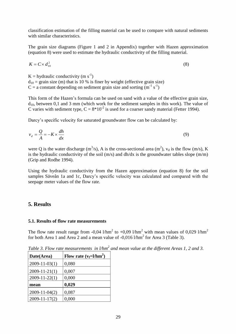
The grain size diagrams (Figure 1 and 2 in Appendix) together with Hazen approximation
(equation 8) were used to estimate the hydraulic conductivity of the filling material.
2
10dCK (8)
K = hydraulic conductivity (m s-1
)
d10 = grain size (m) that is 10 % is finer by weight (effective grain size)
C = a constant depending on sediment grain size and sorting (m-1
s-1
)
This form of the Hazen’s formula can be used on sand with a value of the effective grain size,
d10, between 0,1 and 3 mm (which work for the sediment samples in this work). The value of
C varies with sediment type, C = 8*10-2
is used for a coarser sandy material (Fetter 1994).
Darcy’s specific velocity for saturated groundwater flow can be calculated by:
dx
dhK
A
Qvd (9)
were Q is the water discharge (m3/s), A is the cross-sectional area (m
2), vd is the flow (m/s), K
is the hydraulic conductivity of the soil (m/s) and dh/dx is the groundwater tables slope (m/m)
(Grip and Rodhe 1994).
Using the hydraulic conductivity from the Hazen approximation (equation 8) for the soil
samples Säveån 1a and 1c, Darcy’s specific velocity was calculated and compared with the
seepage meter values of the flow rate.
5. Results
5.1. Results of flow rate measurements
The flow rate result range from -0,04 l/hm2 to +0,09 l/hm
2 with mean values of 0,029 l/hm
2
for both Area 1 and Area 2 and a mean value of -0,016 l/hm2 for Area 3 (Table 3).
Table 3. Flow rate measurements in l/hm2 and mean value at the different Areas 1, 2 and 3.
Date(Area) Flow rate (vf=l/hm2)
2009-11-03(1) 0,080
2009-11-21(1) 0,007
2009-11-22(1) 0,000
mean 0,029
2009-11-04(2) 0,087
2009-11-17(2) 0,000
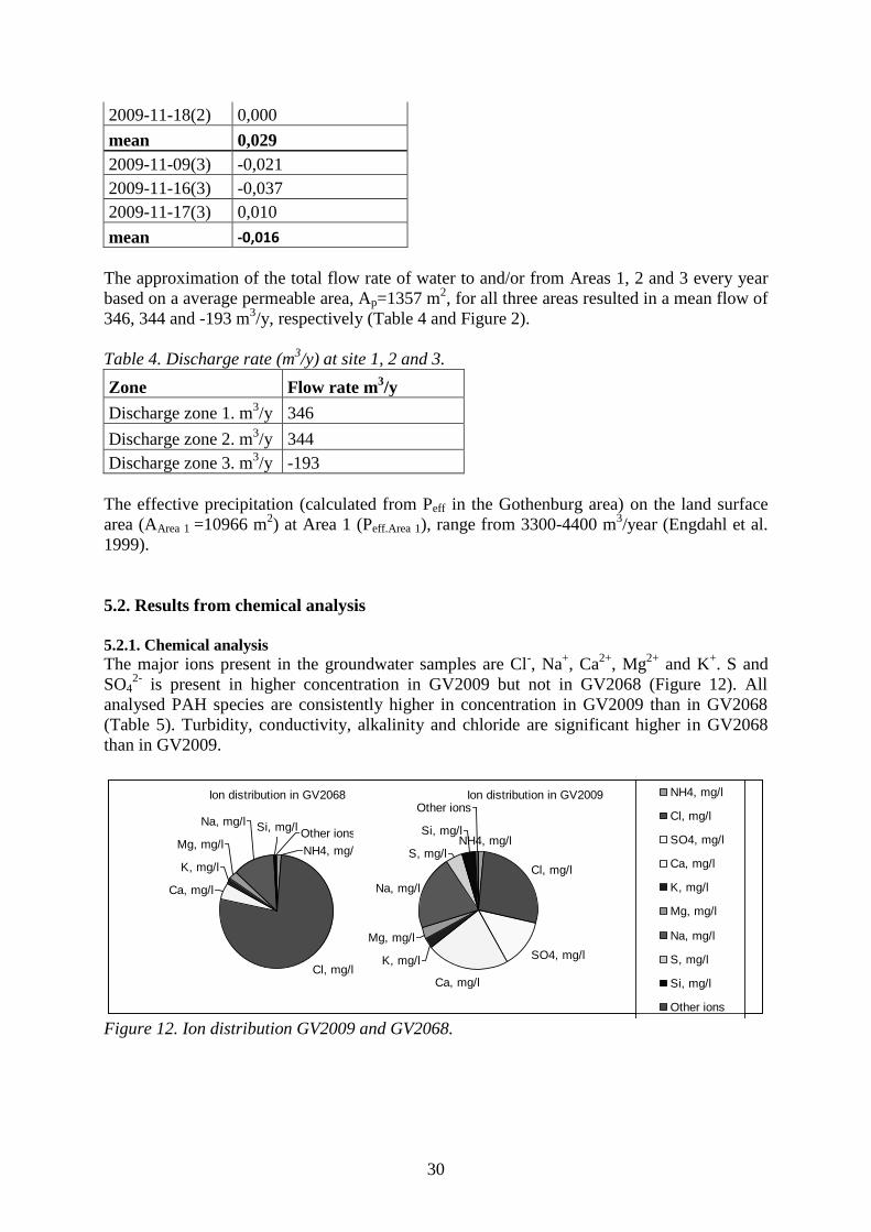
30
2009-11-18(2) 0,000
mean 0,029
2009-11-09(3) -0,021
2009-11-16(3) -0,037
2009-11-17(3) 0,010
mean -0,016
The approximation of the total flow rate of water to and/or from Areas 1, 2 and 3 every year
based on a average permeable area, Ap=1357 m2, for all three areas resulted in a mean flow of
346, 344 and -193 m3/y, respectively (Table 4 and Figure 2).
Table 4. Discharge rate (m3/y) at site 1, 2 and 3.
Zone Flow rate m3/y
Discharge zone 1. m3/y 346
Discharge zone 2. m3/y 344
Discharge zone 3. m3/y -193
The effective precipitation (calculated from Peff in the Gothenburg area) on the land surface
area (AArea 1 =10966 m2) at Area 1 (Peff.Area 1), range from 3300-4400 m
3/year (Engdahl et al.
1999).
5.2. Results from chemical analysis
5.2.1. Chemical analysis
The major ions present in the groundwater samples are Cl-, Na
+, Ca
2+, Mg
2+ and K
+. S and
SO42-
is present in higher concentration in GV2009 but not in GV2068 (Figure 12). All
analysed PAH species are consistently higher in concentration in GV2009 than in GV2068
(Table 5). Turbidity, conductivity, alkalinity and chloride are significant higher in GV2068
than in GV2009.
Figure 12. Ion distribution GV2009 and GV2068.
Ion distribution in GV2068
Cl, mg/l
Ca, mg/l
K, mg/l
Mg, mg/l
Si, mg/l
NH4, mg/l
Other ionsNa, mg/l
Ion distribution in GV2009
NH4, mg/l
Cl, mg/l
SO4, mg/l
Ca, mg/l
K, mg/l
Mg, mg/l
Na, mg/l
S, mg/l
Si, mg/l
Other ions
NH4, mg/l
Cl, mg/l
SO4, mg/l
Ca, mg/l
K, mg/l
Mg, mg/l
Na, mg/l
S, mg/l
Si, mg/l
Other ions
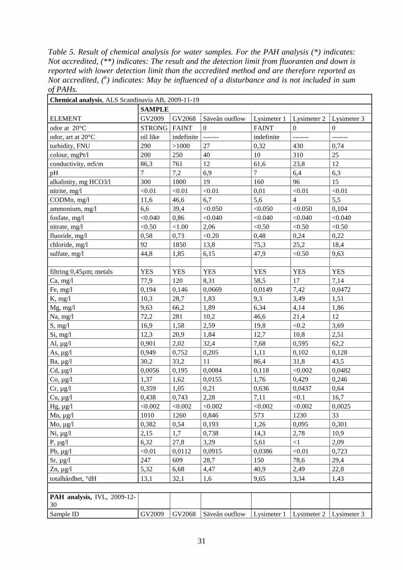
31
Table 5. Result of chemical analysis for water samples. For the PAH analysis (*) indicates:
Not accredited, (**) indicates: The result and the detection limit from fluoranten and down is
reported with lower detection limit than the accredited method and are therefore reported as
Not accredited, (a) indicates: May be influenced of a disturbance and is not included in sum
of PAHs.
Chemical analysis, ALS Scandinavia AB, 2009-11-19
SAMPLE
ELEMENT GV2009 GV2068 Säveån outflow Lysimeter 1 Lysimeter 2 Lysimeter 3
odor at 20°C STRONG FAINT 0 FAINT 0 0
odor, art at 20°C oil like indefinite ------- indefinite ------- -------
turbidity, FNU 290 >1000 27 0,32 430 0,74
colour, mgPt/l 200 250 40 10 310 25
conductivity, mS/m 86,3 761 12 61,6 23,8 12
pH 7 7,2 6,9 7 6,4 6,3
alkalinity, mg HCO3/l 300 1800 19 160 96 15
nitrite, mg/l <0.01 <0.01 <0.01 0,01 <0.01 <0.01
CODMn, mg/l 11,6 46,6 6,7 5,6 4 5,5
ammonium, mg/l 6,6 39,4 <0.050 <0.050 <0.050 0,104
fosfate, mg/l <0.040 0,86 <0.040 <0.040 <0.040 <0.040
nitrate, mg/l <0.50 <1.00 2,06 <0.50 <0.50 <0.50
fluoride, mg/l 0,58 0,73 <0.20 0,48 0,24 0,22
chloride, mg/l 92 1850 13,8 75,3 25,2 18,4
sulfate, mg/l 44,8 1,85 6,15 47,9 <0.50 9,63
filtring 0,45µm; metals YES YES YES YES YES YES
Ca, mg/l 77,9 120 8,31 58,5 17 7,14
Fe, mg/l 0,194 0,146 0,0669 0,0149 7,42 0,0472
K, mg/l 10,3 28,7 1,83 9,3 3,49 1,51
Mg, mg/l 9,63 66,2 1,89 6,34 4,14 1,86
Na, mg/l 72,2 281 10,2 46,6 21,4 12
S, mg/l 16,9 1,58 2,59 19,8 <0.2 3,69
Si, mg/l 12,3 20,9 1,84 12,7 10,8 2,51
Al, µg/l 0,901 2,02 32,4 7,68 0,595 62,2
As, µg/l 0,949 0,752 0,205 1,11 0,102 0,128
Ba, µg/l 30,2 33,2 11 86,4 31,8 43,5
Cd, µg/l 0,0056 0,195 0,0084 0,118 <0.002 0,0482
Co, µg/l 1,37 1,62 0,0155 1,76 0,429 0,246
Cr, µg/l 0,359 1,05 0,21 0,636 0,0437 0,64
Cu, µg/l 0,438 0,743 2,28 7,11 <0.1 16,7
Hg, µg/l <0.002 <0.002 <0.002 <0.002 <0.002 0,0025
Mn, µg/l 1010 1260 0,846 573 1230 33
Mo, µg/l 0,382 0,54 0,193 1,26 0,095 0,301
Ni, µg/l 2,15 1,7 0,738 14,3 2,78 10,9
P, µg/l 6,32 27,8 3,29 5,61 <1 2,09
Pb, µg/l <0.01 0,0112 0,0915 0,0386 <0.01 0,723
Sr, µg/l 247 609 28,7 150 78,6 29,4
Zn, µg/l 5,32 6,68 4,47 40,9 2,49 22,8
totalhårdhet, °dH 13,1 32,1 1,6 9,65 3,34 1,43
PAH analysis, IVL, 2009-12-
30
Sample ID GV2009 GV2068 Säveån outflow Lysimeter 1 Lysimeter 2 Lysimeter 3
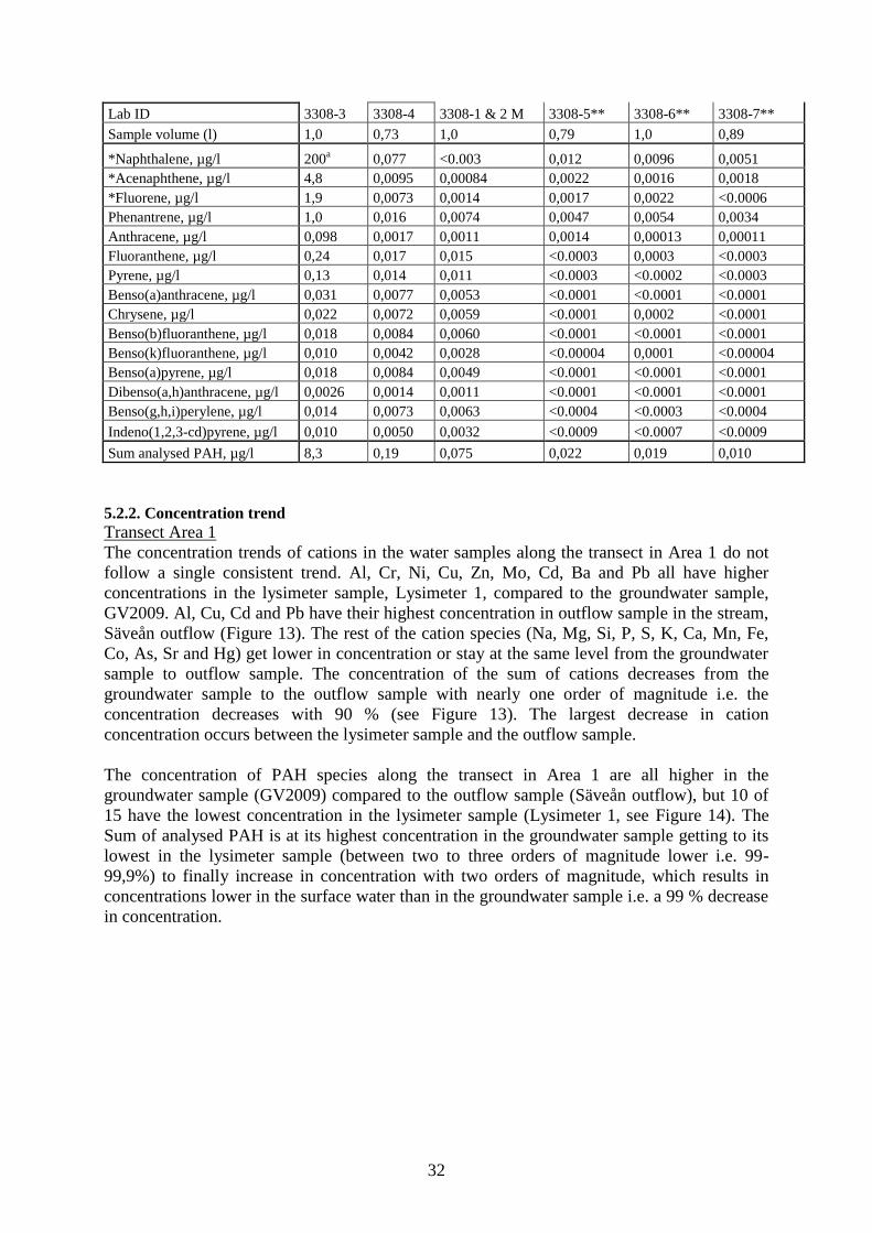
32
Lab ID 3308-3 3308-4 3308-1 & 2 M 3308-5** 3308-6** 3308-7**
Sample volume (l) 1,0 0,73 1,0 0,79 1,0 0,89
*Naphthalene, µg/l 200a 0,077 <0.003 0,012 0,0096 0,0051
*Acenaphthene, µg/l 4,8 0,0095 0,00084 0,0022 0,0016 0,0018
*Fluorene, µg/l 1,9 0,0073 0,0014 0,0017 0,0022 <0.0006
Phenantrene, µg/l 1,0 0,016 0,0074 0,0047 0,0054 0,0034
Anthracene, µg/l 0,098 0,0017 0,0011 0,0014 0,00013 0,00011
Fluoranthene, µg/l 0,24 0,017 0,015 <0.0003 0,0003 <0.0003
Pyrene, µg/l 0,13 0,014 0,011 <0.0003 <0.0002 <0.0003
Benso(a)anthracene, µg/l 0,031 0,0077 0,0053 <0.0001 <0.0001 <0.0001
Chrysene, µg/l 0,022 0,0072 0,0059 <0.0001 0,0002 <0.0001
Benso(b)fluoranthene, µg/l 0,018 0,0084 0,0060 <0.0001 <0.0001 <0.0001
Benso(k)fluoranthene, µg/l 0,010 0,0042 0,0028 <0.00004 0,0001 <0.00004
Benso(a)pyrene, µg/l 0,018 0,0084 0,0049 <0.0001 <0.0001 <0.0001
Dibenso(a,h)anthracene, µg/l 0,0026 0,0014 0,0011 <0.0001 <0.0001 <0.0001
Benso(g,h,i)perylene, µg/l 0,014 0,0073 0,0063 <0.0004 <0.0003 <0.0004
Indeno(1,2,3-cd)pyrene, µg/l 0,010 0,0050 0,0032 <0.0009 <0.0007 <0.0009
Sum analysed PAH, µg/l 8,3 0,19 0,075 0,022 0,019 0,010
5.2.2. Concentration trend
Transect Area 1
The concentration trends of cations in the water samples along the transect in Area 1 do not
follow a single consistent trend. Al, Cr, Ni, Cu, Zn, Mo, Cd, Ba and Pb all have higher
concentrations in the lysimeter sample, Lysimeter 1, compared to the groundwater sample,
GV2009. Al, Cu, Cd and Pb have their highest concentration in outflow sample in the stream,
Säveån outflow (Figure 13). The rest of the cation species (Na, Mg, Si, P, S, K, Ca, Mn, Fe,
Co, As, Sr and Hg) get lower in concentration or stay at the same level from the groundwater
sample to outflow sample. The concentration of the sum of cations decreases from the
groundwater sample to the outflow sample with nearly one order of magnitude i.e. the
concentration decreases with 90 % (see Figure 13). The largest decrease in cation
concentration occurs between the lysimeter sample and the outflow sample.
The concentration of PAH species along the transect in Area 1 are all higher in the
groundwater sample (GV2009) compared to the outflow sample (Säveån outflow), but 10 of
15 have the lowest concentration in the lysimeter sample (Lysimeter 1, see Figure 14). The
Sum of analysed PAH is at its highest concentration in the groundwater sample getting to its
lowest in the lysimeter sample (between two to three orders of magnitude lower i.e. 99-
99,9%) to finally increase in concentration with two orders of magnitude, which results in
concentrations lower in the surface water than in the groundwater sample i.e. a 99 % decrease
in concentration.
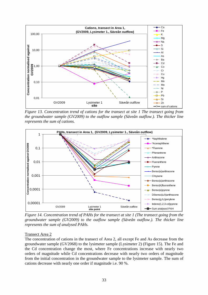
33
Cations, transect in Area 1,
(GV2009, Lysimeter 1., Säveån outflow)
0,01
0,10
1,00
10,00
100,00
GV2009 Lysimeter 1 Säveån outflowsite
Co
nc
en
tra
tio
n n
orm
alis
ed
ag
ain
st
GV
20
09
Ca
Fe
K
Mg
Na
S
Si
Al
As
Ba
Cd
Co
Cr
Cu
Hg
Mn
Mo
Ni
P
Pb
Sr
Zn
sum of cations
Figure 13. Concentration trend of cations for the transect at site 1 The transect going from
the groundwater sample (GV2009) to the outflow sample (Säveån outflow.). The thicker line
represents the sum of cations.
PAHs, transect in Area 1, (GV2009, Lysimeter 1., Säveån outflow)
0,00001
0,0001
0,001
0,01
0,1
1
GV2009 Lysimeter 1 Säveån outflowsite point
Co
nc
en
tra
tio
n n
orm
alis
ed
ag
ain
st
GV
20
09
*Naphthalene
*Acenaphthene
*Fluorene
Phenantrene
Anthracene
Fluoranthene
Pyrene
Benso(a)anthracene
Chrysene
Benso(a)anthracene
Benso(k)fluoranthene
Benso(a)pyrene
Dibenso(a,h)anthracene
Benso(g,h,i)perylene
Indeno(1,2,3-cd)pyrene
Sum analysed PAH
Figure 14. Concentration trend of PAHs for the transect at site 1 (The transect going from the
groundwater sample (GV2009) to the outflow sample (Säveån outflow.). The thicker line
represents the sum of analysed PAHs.
Transect Area 2
The concentration of cations in the transect of Area 2, all except Fe and As decrease from the
groundwater sample (GV2068) to the lysimeter sample (Lysimeter 2) (Figure 15). The Fe and
the Cd concentration change the most, where Fe concentrations increase with nearly two
orders of magnitude while Cd concentrations decrease with nearly two orders of magnitude
from the initial concentration in the groundwater sample to the lysimeter sample. The sum of
cations decrease with nearly one order if magnitude i.e. 90 %.
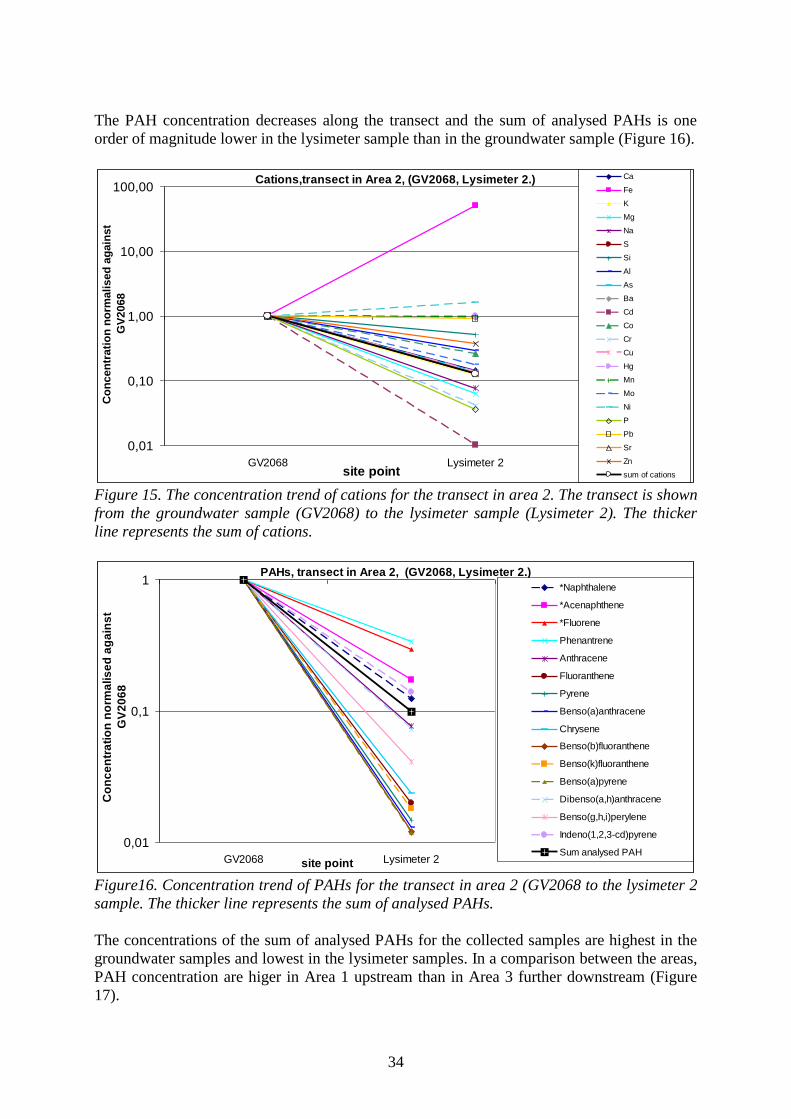
34
The PAH concentration decreases along the transect and the sum of analysed PAHs is one
order of magnitude lower in the lysimeter sample than in the groundwater sample (Figure 16).
Cations,transect in Area 2, (GV2068, Lysimeter 2.)
0,01
0,10
1,00
10,00
100,00
GV2068 Lysimeter 2site point
Co
nc
en
tra
tio
n n
orm
ali
se
d a
gain
st
GV
2068
Ca
Fe
K
Mg
Na
S
Si
Al
As
Ba
Cd
Co
Cr
Cu
Hg
Mn
Mo
Ni
P
Pb
Sr
Zn
sum of cations
Figure 15. The concentration trend of cations for the transect in area 2. The transect is shown
from the groundwater sample (GV2068) to the lysimeter sample (Lysimeter 2). The thicker
line represents the sum of cations.
PAHs, transect in Area 2, (GV2068, Lysimeter 2.)
0,01
0,1
1
GV2068 Lysimeter 2site point
Co
nc
en
tra
tio
n n
orm
alis
ed
ag
ain
st
GV
20
68
*Naphthalene
*Acenaphthene
*Fluorene
Phenantrene
Anthracene
Fluoranthene
Pyrene
Benso(a)anthracene
Chrysene
Benso(b)fluoranthene
Benso(k)fluoranthene
Benso(a)pyrene
Dibenso(a,h)anthracene
Benso(g,h,i)perylene
Indeno(1,2,3-cd)pyrene
Sum analysed PAH
Figure16. Concentration trend of PAHs for the transect in area 2 (GV2068 to the lysimeter 2
sample. The thicker line represents the sum of analysed PAHs.
The concentrations of the sum of analysed PAHs for the collected samples are highest in the
groundwater samples and lowest in the lysimeter samples. In a comparison between the areas,
PAH concentration are higer in Area 1 upstream than in Area 3 further downstream (Figure
17).
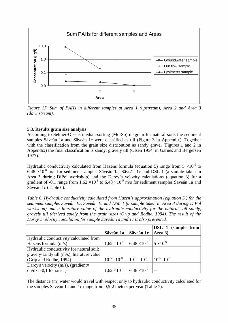
35
Sum PAHs for different samples and Areas
0,0
0,1
1,0
10,0
1 2 3
Area
Co
ncen
trati
on
(μ
g/l
)
Groundwater sample
Out flow sample
Lysimeter sample
Figure 17. Sum of PAHs in different samples at Area 1 (upstream), Area 2 and Area 3
(downstream).
5.3. Results grain size analysis
According to Selmer-Olsens median-sorting (Md-So) diagram for natural soils the sediment
samples Säveån 1a and Säveån 1c were classified as till (Figure 3 in Appendix). Together
with the classification from the grain size distribution as sandy gravel (Figures 1 and 2 in
Appendix) the final classification is sandy, gravely till (Olsen 1954, in Garnes and Bergersen
1977).
Hydraulic conductivity calculated from Hazens formula (equation 5) range from 5 ×10⁻⁹
to
6,48 ×10⁻⁸
m/s for sediment samples Säveån 1a, Säveån 1c and DSL 1 (a sample taken in
Area 3 during DiPol workshop) and the Darcy’s velocity calculations (equation 3) for a
gradient of -0,1 range from 1,62 ×10⁻⁹
to 6,48 ×10⁻⁹
m/s for sediment samples Säveån 1a and
Säveån 1c (Table 6).
Table 6. Hydraulic conductivity calculated from Hazen’s approximation (equation 5.) for the
sediment samples Säveån 1a, Säveån 1c and DSL 1 (a sample taken in Area 3 during DiPol
workshop) and a literature value of the hydraulic conductivity for the natural soil sandy,
gravely till (derived solely from the grain size) (Grip and Rodhe, 1994). The result of the
Darcy’s velocity calculation for sample Säveån 1a and 1c is also presented.
The distance (m) water would travel with respect only to hydraulic conductivity calculated for
the samples Säveån 1a and 1c range from 0,5-2 meters per year (Table 7).
Säveån 1a Säveån 1c
DSL 1 (sample from
Area 3)
Hydraulic conductivity calculated from
Hazens formula (m/s) 1,62 ×10⁻⁸
6,48 ×10⁻⁸
5 ×10⁻⁹
Hydraulic conductivity for natural soil:
gravely-sandy till (m/s), literature value
(Grip and Rodhe, 1994) 10-5
- 10-8
10-5
- 10-8
10-5
-10-8
Darcy's velocity (m/s), (gradient=
dh/dx=-0,1 for site 1) 1,62 ×10⁻⁹
6,48 ×10⁻⁹
--
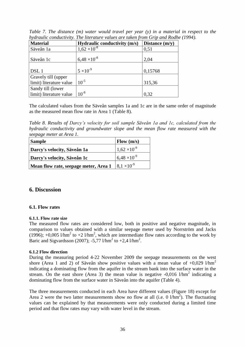
36
Table 7. The distance (m) water would travel per year (y) in a material in respect to the
hydraulic conductivity. The literature values are taken from Grip and Rodhe (1994).
Material Hydraulic conductivity (m/s) Distance (m/y)
Säveån 1a 1,62 ×10⁻⁸
0,51
Säveån 1c 6,48 ×10⁻⁸
2,04
DSL 1 5 ×10⁻⁹
0,15768
Gravely till (upper
limit) literature value 10-5
315,36
Sandy till (lower
limit) literature value 10-8
0,32
The calculated values from the Säveån samples 1a and 1c are in the same order of magnitude
as the measured mean flow rate in Area 1 (Table 8).
Table 8. Results of Darcy’s velocity for soil sample Säveån 1a and 1c, calculated from the
hydraulic conductivity and groundwater slope and the mean flow rate measured with the
seepage meter at Area 1.
Sample Flow (m/s)
Darcy's velocity, Säveån 1a 1,62 ×10⁻⁹
Darcy's velocity, Säveån 1c 6,48 ×10⁻⁹
Mean flow rate, seepage meter, Area 1 8,1 ×10⁻⁹
6. Discussion
6.1. Flow rates
6.1.1. Flow rate size
The measured flow rates are considered low, both in positive and negative magnitude, in
comparison to values obtained with a similar seepage meter used by Norrström and Jacks
(1996); +0,005 l/hm2 to +2 l/hm
2, which are intermediate flow rates according to the work by
Baric and Sigvardsson (2007); -5,77 l/hm2 to +2,4 l/hm
2.
6.1.2 Flow direction
During the measuring period 4-22 November 2009 the seepage measurements on the west
shore (Area 1 and 2) of Säveån show positive values with a mean value of +0,029 l/hm2
indicating a dominating flow from the aquifer in the stream bank into the surface water in the
stream. On the east shore (Area 3) the mean value is negative -0,016 l/hm2 indicating a
dominating flow from the surface water in Säveån into the aquifer (Table 4).
The three measurements conducted in each Area have different values (Figure 18) except for
Area 2 were the two latter measurements show no flow at all (i.e. 0 l/hm2). The fluctuating
values can be explained by that measurements were only conducted during a limited time
period and that flow rates may vary with water level in the stream.
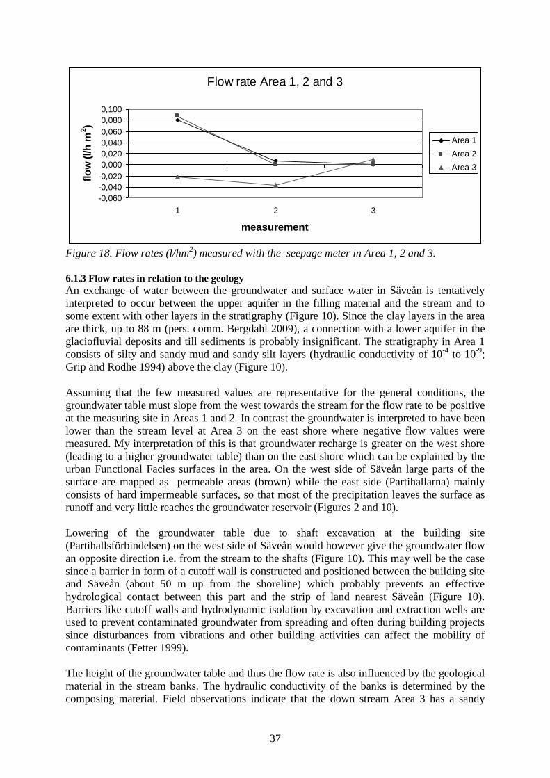
37
Flow rate Area 1, 2 and 3
-0,060
-0,040
-0,020
0,000
0,020
0,040
0,060
0,080
0,100
1 2 3
measurement
flo
w (
l/h
m2)
Area 1
Area 2
Area 3
Figure 18. Flow rates (l/hm
2) measured with the seepage meter in Area 1, 2 and 3.
6.1.3 Flow rates in relation to the geology
An exchange of water between the groundwater and surface water in Säveån is tentatively
interpreted to occur between the upper aquifer in the filling material and the stream and to
some extent with other layers in the stratigraphy (Figure 10). Since the clay layers in the area
are thick, up to 88 m (pers. comm. Bergdahl 2009), a connection with a lower aquifer in the
glaciofluvial deposits and till sediments is probably insignificant. The stratigraphy in Area 1
consists of silty and sandy mud and sandy silt layers (hydraulic conductivity of 10-4
to 10-9
;
Grip and Rodhe 1994) above the clay (Figure 10).
Assuming that the few measured values are representative for the general conditions, the
groundwater table must slope from the west towards the stream for the flow rate to be positive
at the measuring site in Areas 1 and 2. In contrast the groundwater is interpreted to have been
lower than the stream level at Area 3 on the east shore where negative flow values were
measured. My interpretation of this is that groundwater recharge is greater on the west shore
(leading to a higher groundwater table) than on the east shore which can be explained by the
urban Functional Facies surfaces in the area. On the west side of Säveån large parts of the
surface are mapped as permeable areas (brown) while the east side (Partihallarna) mainly
consists of hard impermeable surfaces, so that most of the precipitation leaves the surface as
runoff and very little reaches the groundwater reservoir (Figures 2 and 10).
Lowering of the groundwater table due to shaft excavation at the building site
(Partihallsförbindelsen) on the west side of Säveån would however give the groundwater flow
an opposite direction i.e. from the stream to the shafts (Figure 10). This may well be the case
since a barrier in form of a cutoff wall is constructed and positioned between the building site
and Säveån (about 50 m up from the shoreline) which probably prevents an effective
hydrological contact between this part and the strip of land nearest Säveån (Figure 10).
Barriers like cutoff walls and hydrodynamic isolation by excavation and extraction wells are
used to prevent contaminated groundwater from spreading and often during building projects
since disturbances from vibrations and other building activities can affect the mobility of
contaminants (Fetter 1999).
The height of the groundwater table and thus the flow rate is also influenced by the geological
material in the stream banks. The hydraulic conductivity of the banks is determined by the
composing material. Field observations indicate that the down stream Area 3 has a sandy
38
material while the upstream Area 1 has a more clay-rich filling material in direct proximity to
the stream. The hydraulic conductivity calculated from Hazens formula (equation 5) is
slightly lower for the soil sample (DSL1) taken in Area 3 (during DiPol workshop) than for
the samples taken at Area 1 (Table 7), but even still around the same value and very low.
Filling material is a heterogeneous material and the slight difference in the approximated
conductivity can be due to this.
The effective precipitation, Peff; for the area within the cutoff wall barrier and the Säveån
stream in Area 1 is 3300-4400 m3/year and the measured flow rate for the same area is 346
m3/year (Figure 10). The amount of surface runoff water in this area would then be about
3000-4000 m3/year if the flow rate measurements are valid. The mean value of the measured
flow rate and the value of Darcys’s velocity calculated for Area 1 result in the same order of
magnitude (8,1 ×10⁻⁹
and 1,62 ×10⁻⁹ to 6,48 ×10
-9 m/s, respectively) and therefore indicate
that the flow measurements are relevant. If Darcy’s velocity (m/s) for the sediment samples
Säveån 1a and 1c is recalculated to m3/year for the area of the permeable layer in Area 1 it
results in 69-277 m3/y (Table 9). The runoff water can either enter a drainage system or reach
Säveån directly.
Table 9. Darcy’s velocity compared with flow rate for the permeable layer in Area 1 given in
m3/year.
Area 1
Velocities for permeable
area in Area 1
Volume/year for permeable
area (m3/y)
Sediment samples
(Säveån 1a and 1c) Darcys velocity 69-277
Flow rate
measurement Mean flow rate 346
6.1.4 The flow rates contribution to the spreading of pollutants
In a source and sink view having only the flow situation from the banks in mind the west
shore with its small aquifer system acts as a source while the east shore with negative flow
rate acts as a sink. Together Area 1 and 2 contributes with 1,6 ×10⁻⁸
m/s of groundwater flow
to Säveåns mean annual discharge, 18 m3/s, which is a 8,9×10
-8 % of it. Concentrations are
however higher in the water leaving the banks than in Säveån (Figures 13-16).
During the field period rapid fluctuations of the water level in Säveån was noticed and the
question of its potential effect on the spreading of pollutants from the banks arouse (see
Figure 1). Does the fluctuation of the stream water level contribute to the spreading of
pollutants to Säveån more than the groundwater flow does?
6.2. Water chemistry and pollutants at the study site
According to information gathered during this project the pollution situation of the ground in
the study area shows that pollution is more widespread at the west shore of Säveån than along
the east shore and contains compounds that are more severe (oils, PAHs and metals and
cyanides) which source probably comes from the filling material. The pollution at the east
shore is characteristic for the activities conducted at a marshalling yard (e.g. arsenic used for
impregnating rail road ties, metals, oils and creosotes). The east shore can be characterised
more as a point source since previous and ongoing activities are known while the west shore
has a more diffuse source related to the filling material taken from other sources. Both shores
have a diffuse pollution source due to heavy traffic, truck traffic communication at the
39
wholesaler area (Partihallarna the east shore) and the Marieholmsleden highway (the E45
road) near the west shore.
6.2.1. Concentrations compared to guideline values
Comparing the chemical concentrations and the parameters analysed with the same guideline
values used in Tyréns AB report (2009) all values except for the conductivity (guide line
value, 50 mS/m; from Naturvårdsverket 1999) in sample GV2009, GV2068 and Lysimeter 1
show values beneath the guideline values i.e. acceptable values (Tyréns AB 2009: including
guideline values from the Swedish EPA (Naturvårdsverket) and KEMAKTA (Table 10).
Table 10. Guideline values used in Tyréns AB report (2009).
The guidline values used by Tyréns AB for different chemical parameters.
Parameter pH and conductivity AS, Cd, Cu, Cr and
Ni
Co and Zn For Pb and
different
hydrocarbons
Guideline value
used
The Swedish EPA’s
guideline values for
natural concentration
range for
groundwater.
The Swedish EPA’s
classification of the
state of contaminated
groundwater based
on a health-based
limit for drinking
water.
Dutch intervention
value.
Kemaktas
suggested
guideline values
for substances in
groundwater near
gas-stations for
the exposure route
of environmental
hazards in surface
waters.
The guideline value for ―The Sum of other PAHs‖ (used in Tyréns AB report 2009) is set to
100 μg/l and is accounted for a typical composition of PAHs including: Naphthalene (40%),
Acenaphthene (20%), Flourene (15%), Phenatrene (10%) and Floranthene (5%) according to
KEMAKTAs guideline values (Elert 2006). This is exceeded in the sample GV2009 were it
reaches a value of 207,93 μg/l, but Naphthalene contributes with 200 μg/l according to the
laboratory results from IVL laboratory. IVLs explanation is that this sample can have been
disturbed since it is extremely high compared to the other samples and species analysed and
should perhaps not be taken into account (Table 5). In that case no ―sum of other PAH‖
concentrations in the samples taken during this project exceed the guideline values by
KEMAKTA (Elert 2006). KEMAKTA’s guidelines for surface water concerning pollution
from groundwater are set at a value that accounts for the concentration after dissolution of the
potential pollution in the surface water (Elert 2006). Tyréns AB have also measured values of
―The sum of other PAHs‖ over the guideline value (100 μg/l) for observation well GV2009
(Figure 19, Tyréns AB 2009).
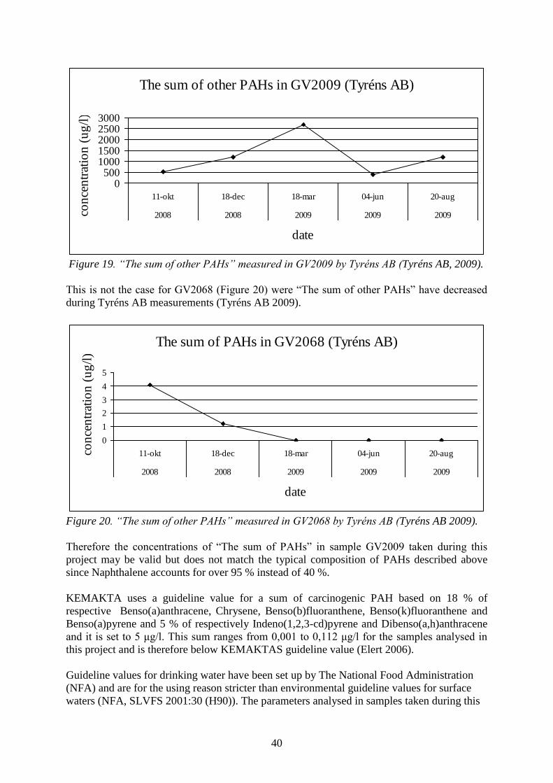
40
The sum of other PAHs in GV2009 (Tyréns AB)
0500
10001500200025003000
11-okt 18-dec 18-mar 04-jun 20-aug
2008 2008 2009 2009 2009
date
con
cen
trat
ion
(u
g/l
)
Figure 19. “The sum of other PAHs” measured in GV2009 by Tyréns AB (Tyréns AB, 2009).
This is not the case for GV2068 (Figure 20) were ―The sum of other PAHs‖ have decreased
during Tyréns AB measurements (Tyréns AB 2009).
The sum of PAHs in GV2068 (Tyréns AB)
0
1
2
3
4
5
11-okt 18-dec 18-mar 04-jun 20-aug
2008 2008 2009 2009 2009
date
con
cen
trat
ion
(u
g/l
)
Figure 20. “The sum of other PAHs” measured in GV2068 by Tyréns AB (Tyréns AB 2009).
Therefore the concentrations of ―The sum of PAHs‖ in sample GV2009 taken during this
project may be valid but does not match the typical composition of PAHs described above
since Naphthalene accounts for over 95 % instead of 40 %.
KEMAKTA uses a guideline value for a sum of carcinogenic PAH based on 18 % of
respective Benso(a)anthracene, Chrysene, Benso(b)fluoranthene, Benso(k)fluoranthene and
Benso(a)pyrene and 5 % of respectively Indeno(1,2,3-cd)pyrene and Dibenso(a,h)anthracene
and it is set to 5 μg/l. This sum ranges from 0,001 to 0,112 μg/l for the samples analysed in
this project and is therefore below KEMAKTAS guideline value (Elert 2006).
Guideline values for drinking water have been set up by The National Food Administration
(NFA) and are for the using reason stricter than environmental guideline values for surface
waters (NFA, SLVFS 2001:30 (H90)). The parameters analysed in samples taken during this
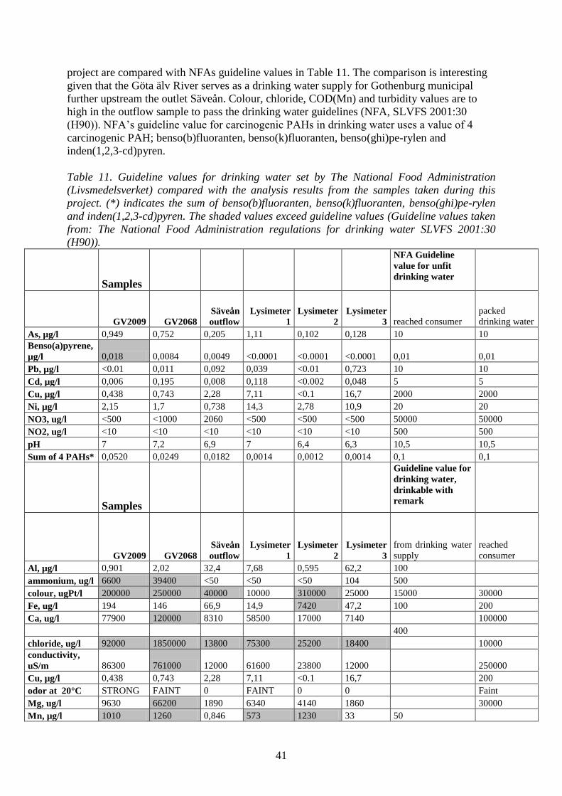
41
project are compared with NFAs guideline values in Table 11. The comparison is interesting
given that the Göta älv River serves as a drinking water supply for Gothenburg municipal
further upstream the outlet Säveån. Colour, chloride, COD(Mn) and turbidity values are to
high in the outflow sample to pass the drinking water guidelines (NFA, SLVFS 2001:30
(H90)). NFA’s guideline value for carcinogenic PAHs in drinking water uses a value of 4
carcinogenic PAH; benso(b)fluoranten, benso(k)fluoranten, benso(ghi)pe-rylen and
inden(1,2,3-cd)pyren.
Table 11. Guideline values for drinking water set by The National Food Administration
(Livsmedelsverket) compared with the analysis results from the samples taken during this
project. (*) indicates the sum of benso(b)fluoranten, benso(k)fluoranten, benso(ghi)pe-rylen
and inden(1,2,3-cd)pyren. The shaded values exceed guideline values (Guideline values taken
from: The National Food Administration regulations for drinking water SLVFS 2001:30
(H90)).
Samples
NFA Guideline
value for unfit
drinking water
GV2009 GV2068
Säveån
outflow
Lysimeter
1
Lysimeter
2
Lysimeter
3 reached consumer
packed
drinking water
As, µg/l 0,949 0,752 0,205 1,11 0,102 0,128 10 10
Benso(a)pyrene,
µg/l 0,018 0,0084 0,0049 <0.0001 <0.0001 <0.0001 0,01 0,01
Pb, µg/l <0.01 0,011 0,092 0,039 <0.01 0,723 10 10
Cd, µg/l 0,006 0,195 0,008 0,118 <0.002 0,048 5 5
Cu, µg/l 0,438 0,743 2,28 7,11 <0.1 16,7 2000 2000
Ni, µg/l 2,15 1,7 0,738 14,3 2,78 10,9 20 20
NO3, ug/l <500 <1000 2060 <500 <500 <500 50000 50000
NO2, ug/l <10 <10 <10 <10 <10 <10 500 500
pH 7 7,2 6,9 7 6,4 6,3 10,5 10,5
Sum of 4 PAHs* 0,0520 0,0249 0,0182 0,0014 0,0012 0,0014 0,1 0,1
Samples
Guideline value for
drinking water,
drinkable with
remark
GV2009 GV2068
Säveån
outflow
Lysimeter
1
Lysimeter
2
Lysimeter
3
from drinking water
supply
reached
consumer
Al, µg/l 0,901 2,02 32,4 7,68 0,595 62,2 100
ammonium, ug/l 6600 39400 <50 <50 <50 104 500
colour, ugPt/l 200000 250000 40000 10000 310000 25000 15000 30000
Fe, ug/l 194 146 66,9 14,9 7420 47,2 100 200
Ca, ug/l 77900 120000 8310 58500 17000 7140 100000
400
chloride, ug/l 92000 1850000 13800 75300 25200 18400 10000
conductivity,
uS/m 86300 761000 12000 61600 23800 12000 250000
Cu, µg/l 0,438 0,743 2,28 7,11 <0.1 16,7 200
odor at 20°C STRONG FAINT 0 FAINT 0 0 Faint
Mg, ug/l 9630 66200 1890 6340 4140 1860 30000
Mn, µg/l 1010 1260 0,846 573 1230 33 50
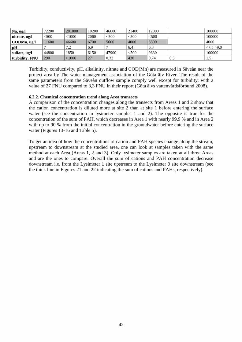
42
Na, ug/l 72200 281000 10200 46600 21400 12000 100000
nitrate, ug/l <500 <1000 2060 <500 <500 <500 100000
CODMn, ug/l 11600 46600 6700 5600 4000 5500 4000
pH 7 7,2 6,9 7 6,4 6,3 <7,5 >9,0
sulfate, ug/l 44800 1850 6150 47900 <500 9630 100000
turbidity, FNU 290 >1000 27 0,32 430 0,74 0,5 1,5
Turbidity, conductivity, pH, alkalinity, nitrate and COD(Mn) are measured in Säveån near the
project area by The water management association of the Göta älv River. The result of the
same parameters from the Säveån outflow sample comply well except for turbidity; with a
value of 27 FNU compared to 3,3 FNU in their report (Göta älvs vattenvårdsförbund 2008).
6.2.2. Chemical concentration trend along Area transects
A comparison of the concentration changes along the transects from Areas 1 and 2 show that
the cation concentration is diluted more at site 2 than at site 1 before entering the surface
water (see the concentration in lysimeter samples 1 and 2). The opposite is true for the
concentration of the sum of PAH, which decreases in Area 1 with nearly 99,9 % and in Area 2
with up to 90 % from the initial concentration in the groundwater before entering the surface
water (Figures 13-16 and Table 5).
To get an idea of how the concentrations of cation and PAH species change along the stream,
upstream to downstream at the studied area, one can look at samples taken with the same
method at each Area (Areas 1, 2 and 3). Only lysimeter samples are taken at all three Areas
and are the ones to compare. Overall the sum of cations and PAH concentration decrease
downstream i.e. from the Lysimeter 1 site upstream to the Lysimeter 3 site downstream (see
the thick line in Figures 21 and 22 indicating the sum of cations and PAHs, respectively).
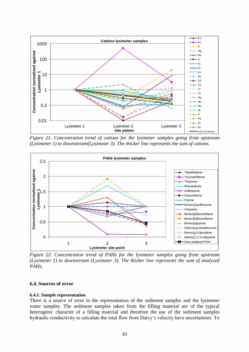
43
Cations lysimeter samples
0,01
0,1
1
10
100
1000
Lysimeter 1 Lysimeter 2 Lysimeter 3 site points
Co
ncen
trati
on
no
rmali
sed
ag
ain
st
Lysim
ete
r 1
Ca
Fe
K
Mg
Na
S
Si
Al
As
Ba
Cd
Co
Cr
Cu
Hg
Mn
Mo
Ni
P
Pb
Sr
Zn
sum of cations
Figure 21. Concentration trend of cations for the lysimeter samples going from upstream
(Lysimeter 1) to downstream(Lysimeter 3). The thicker line represents the sum of cations.
PAHs lysimeter samples
0
0,5
1
1,5
2
2,5
1 2 3Lysimeter site point
Co
nc
en
tra
tio
n n
orm
alis
ed
ag
ain
st
Ly
sim
ete
r 1
*Naphthalene
*Acenaphthene
*Fluorene
Phenantrene
Anthracene
Fluoranthene
Pyrene
Benso(a)anthracene
Chrysene
Benso(b)fluoranthene
Benso(k)fluoranthene
Benso(a)pyrene
Dibenso(a,h)anthracene
Benso(g,h,i)perylene
Indeno(1,2,3-cd)pyrene
Sum analysed PAH
Figure 22. Concentration trend of PAHs for the lysimeter samples going from upstream
(Lysimeter 1) to downstream (Lysimeter 3). The thicker line represents the sum of analysed
PAHs.
6.4. Sources of error
6.4.1. Sample representation
There is a source of error in the representation of the sediment samples and the lysimeter
water samples. The sediment samples taken from the filling material are of the typical
heterogenic character of a filling material and therefore the use of the sediment samples
hydraulic conductivity to calculate the total flow from Darcy’s velocity have uncertainties. To
44
get a representative sample of the filling material several samples are required (time and
budget dependent).
During the sampling time that was required for the lysimeter samples (24 hours or more) the
water level in Säveån sometimes changed up to 2 m vertically. From being installed 1 m up
from the shoreline in level with the groundwater table the lysimeter can occasionally be
covered by 1 m or more of surface water from Säveån, probably influencing the sample taken
by the suction lysimeter. This gives an uncertainty of what is sampled during the lysimeter
sampling. The volume proportion sampled from the interface between groundwater and
surface water and the proportion from the surface water due to bank storage during high water
levels is unknown in each sample. This source of error questions the comparability of the
three lysimeter samples, since they are sampled at different dates/occasions and therefore the
fluctuation in water level could have been different.
6.4.2. Contamination risks of samples
A contaminations risk of water samples exists from the sampling to the analysis in the
laboratory and depends on equipment, handling, storage of samples and storage time before
reaching the laboratories. If the equipment is not clean or is made of reactive materials this is
a source of error. Careless handling of samples is another source of error, exposing them to
high temperatures or oxygen can change the chemical composition. The bladder pump used
for sampling the groundwater was constructed of inert material and the sample bottles were
washed in strong acid. Water samples were stored below +10 ºC within 24 hours until they
were sent to the laboratories.
6.5. Conclusions
The flow rates at the studied part of Säveån are low compared to other studies that used the
same measuring method. There is a positive flow rate value in Areas 1 and 2, indicating a
flow of groundwater from the upper aquifer in the filling material into the Säveån stream on
the west shore. A negative value in Area 3 indicates a flow of water from Säveån into the
bank on the east shore. Greater groundwater recharge on the west shore than on the east shore
due to differences in Functional Facies surfaces can be the explanation
The constructed barrier and excavated shafts isolates most of the hydrogeological system at
the building area from Säveån making the small strip of land on the east side of the barrier
into a separate aquifer. This gives a situation of groundwater flow towards Säveån on the west
side of the barrier. The strip of land on the east side of the barrier is the part contributing with
water through groundwater flow and runoff to Säveån along Areas 1 and 2.
The concentration of both the sum of cations and PAHs analysed decline from the
groundwater to the surface water. The analysed chemical parameters all meet the guideline
values set by the Swedish EPA and KEMAKTA used in Tyréns AB report except for the
conductivity in some samples and for Naphthalene (if valid) in GV2009.
45
7. Acknowledgements
I would like to thank my supervisors Charlotte Sparrenbom (SGI) and professor Rodney
Stevens (GU) for great support and valuable advice through out this project. Leif Cliffordson
(Vägverket) is acknowledged for giving valuable site information and data. I would also like
to thank Thomas Rihm (SGI) for helping out with disposing and organising the water samples
and for good advice.
Thank you Dr Mark Jonson (GU) for critical examining my thesis and giving valuable
comments.
Thank you master student Anoushe Abdolahpour at the Department of Earth Science for
reviewing and discussing my thesis.
I thank the Swedish Geotechnical institute (SGI) for providing field equipment and financing
the chemical analysis.
46
8. References
Adrielsson, P. och Fredén C. (1987), Beskrivning till jordartskartan Marstrand SO/Göteborg
SV, Sveriges Geologiska Undersökning, Serie Ae Nr. 72, Uppsala, 103 pp.
Baric D. och Sigvardsson E. (2007), Distribution and mobilisation of arsenic in Red River
delta aquifers, Vietnam, Earth Sciences Center, Göteborg University, B529 Göteborg,
Sweden, 83 pp.
Bergdahl K., pers.comm. (2009), Map over study area, Stadsbyggnadskontoret Göteborg.
Birgerson B. Sterner O. and Zimerson E. (2009), Kemiska hälsorisker, Toxikologi i kemiskt
perspective, Liber, Malmö, Sweden, 320 pp.
City office of Gothenburg (2006), Extrema vädersituationer -hur väl rustat är Göteborg?-,
Göteborgs Stad, Stadskansliet, 63 pp.
Cliffordson L., pers.comm. (2009), Drilling profiles in sediment, Miljösamordnare,
Partihallförbindelsen, Vägverket, Gothenburg, Sweden.
Digitala kartbiblioteket (2010), https://butiken.metria.se/digibib/index.php (2010-01-16).
DiPol (2010), http://www.tu-harburg.de/iue/dipol.html (2010-02-08).
DiPol workshop (2009); Abdollahpour A., Lundgren A., Robijn A., Schenholm F., Zachrisson
E., Univesity of Gothenburg, Göteborg.
Drever J. I. (1997), The geochemistry of natural waters: surface and groundwater
environments, Prentice-Hall, New Jersey, 436 pp.
Eklund H. S. (2002), Hydrogeologiska typmiljöer: verktyg för bedömning av
grundvattenkvalitet, identifiering av grundvattenförekomster samt underlag för
riskhantering längs vägar, CTH, Geologiska institutionen. A, 101, Göteborg.
Elert M. (2006), Riktvärden för ämnen i grundvatten vid bensinstationer, KEMAKTA AR
2005-31.
Eniro maps (2009), http://kartor.eniro.se/
Engdahl M., Fogdestam B. och Engqvist P. (1999), Beskrivning till karta över grundvatten i
Västra Götalands län, västra delen, f.d. Göteborgs och Bohus län, Sveriges Geologiska
Undersökning , Serie Ah Nr. 12, Uppsala, 52 pp.
Fetter C. W. (1999), Contaminant hydrogeology, Prentice-Hall Inc., New Jersey, 500 pp.
Fetter C. W. (1994), Applied hydrogeology, Prentice-Hall Inc., New Jersey, 598 pp.
Fréden C. (2002), Berg och jord, Sveriges Nationalatlas (SNA), 208 pp.
Garnes K. and Bergersen O. F. (1977), Distribution and genesis of tills in central south
Norway, Boreas, 6, 135-147.
Grip H. and Rodhe A. (1994), Vattnets väg från regn till bäck, Hallgren och Fallgren
Studieförlag AB, Carlshamn Tryck och Media AB, Karlshamn, 155 pp.
Göta älvs vattenvårdsförbund (2010), http://www.gotaalvvvf.org/ (2010-01-08).
Göta älvs vattenvårdsförbund (2008), DEL B Säveån, Ingående i rapport avseende 2008 års
vattendragskontroll, 27 pp.
Göta älvs vattenvårdsförbund (2005), Fakta om Göta älv, En beskrivning av Göta älv och dess
omgivning, 140 pp.
Hitchon B., Perkins E. H. and Gunter W. D. (1999), Introduction to ground water
geochemistry, Alberta Research Council Inc., Canada, 310 pp.
Hultén, A-M. (1997), Grundvatten i urban miljö, Grundvattnets nivåvariationer i de övre
marklagren i Göteborg, CTH, Geologiska institutionen, Publ. A 85, Göteborg
Kemikalieinspektionen 2010, http://www.kemi.se/templates/Page____4439.aspx 2010-05-15
(2010-05-15)
47
Knutsson G. and Morfeldt C-O. (2002), Grundvatten, teori och tillämpning, third edition,
Svenskt Tryck AB, Stockholm, 227 pp.
Lång L.-O., Bergstedt-Söderström A. och Ojala L. (2005), Förslag till distriktsvis inventering
av grundvattenförekomster, SGU-rapport 2005:3.
Länsstyrelsernas GIS tjänster 2010, http://www.gis.lst.se/vattenkartan/htm/viewer.asp (2010-
05-16).
Magnusson E. (1978), Beskrivning till jordartskartan Göteborg SO, Sveriges Geologiska
Undersökning, Serie Ae Nr.26, Stockholm, 154 pp.
Naturvårdsverket (2010), http://www.naturvardsverket.se/sv/ (2010-01-13, 2010-02-10).
Naturvårdsverket (1999), Bedömningsgrunder för miljökvalitet - Metodik för inventering av
förorenade områden, SNV rapport 4918, 152 pp.
Norin M. (2004), Subsurface environmental impact in urban areas: shallow groundwater
composition, corrosion of soil-buried constructions, and leachates from reclaimed
asphalt pavement, Ph.D. series: 2081, Chalmers tekniska högskola, Gothenburg, 104 pp.
Norrström and Jacks (1996), Water path ways and chemistry at the groundwater/surface water
interface to Lake Skjervatjern, Norway, Water Resources Research, 32, 2221-2229.
Olsen S. R. (1954), Om norske jordarters variasjon i korngradering og plastisitet. Nor. Geolo.
Unders, 186, 102 pp (Ref. in Garnes and Bergersen 1977).
SAKAB homepage: http://www.sakab.se/templates/Page.aspx?id=451 (2010-02-05).
SGU (2009), Map generator http://maps.sgu.se/sguinternetmaps/jord/viewer.htm (2010-01-
16).
SGU (1998), Karta över grundvattnet i västra Götalands län, västra delen f.d. Göteborgs och
Bohus län, Serie Ah, Nr. 12.
Samuelsson A.MKB of E6 / VÄG 45 / E20 Marieholmsförbindelsen,
ARBETSPLAN, Beställare: Vägverket, Region Väst, Konsult: WSP
Sammhällsbyggnad, 95 pp.
Stevens, R. L.1, Andersson-Sköld, Yvonne
2, Cato, Ingemar
1, Göransson, Gunnel
2, Marie,
Frogner-Kockum, Paul3, Haeger-Eugensson
4, Lind, Bo
2, Persson, Karin
4, Sparrenbom,
Charlotte3, Rihm, Thomas
2, Abdollapouri, Anousheh
1, Blom, Maria
1, Lundgren, Anna
1,
Zachrisson, Erik1 (2009), Sources and transport pathways of diffuse urban pollution in
Göteborg (DiPol project), Poster presentation for Environmental Impact and Challenges
= ER:4
Stevens R. L. and Hellgren L-G. (1990), A generalized lithofacies model for glaciomarine and
marine sequences in Göteborg area, Sweden, Geologiska Föreningens i Stockholm
Förhandlingar, 112, 89-105
Sjöfartsverket (2010), http://www.sjofartsverket.se/templates/SFVXPage____597.aspx
(2010-02-11).
SMHI OceanWeb (2010), http://produkter.smhi.se/OceanWeb/ (2010-02-11).
Stål T. and Wedel P. (1984), Handboken Bygg , LiberTryck, Stockholm, 603 pp.
Tyréns AB (2009), Yt- och grundvattenkontroll längs Säveån, rapport Nr 5, Uppdrag:
Väg45/E20 Partihallförbindelsen, Beställare: Vägverket Region Väst, 18 pp.
Von Arbin S., Bergstrand T., Bersgström L., Danielsson R., Egriell N., Herklint M., Lithander
L., Nilsson A. and Olsson L. (2008), Säveåns landskap, En natur- och kulturmiljöstudie,
Västarvet rapport, Cela Grafiska AB, Vänersborg, 95 pp.
vanLoon G. W. and Duffy S. J. (2005), Environmental chemistry a global perspective, Oxford
University Press inc., New York, 515 pp.
Västarvet (2010),
http://www.vastarvet.se/kulturvast_templates/Kultur_ArticlePage.aspx?id=38003 (2010-
01-08).

48
Västra Götalands län (2010), http://www.lst.se/vastragotaland/Projektwebbar/saveaprojektet/
(2010-01-08).
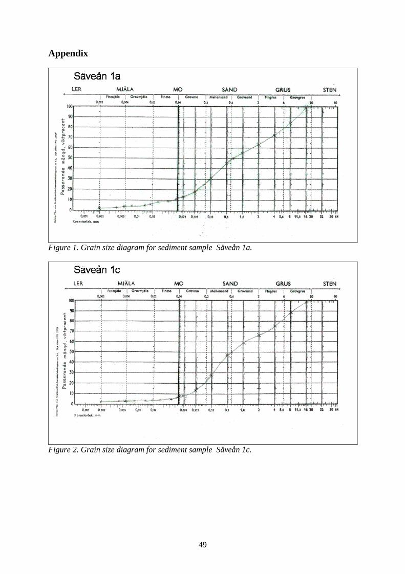
49
Appendix
Figure 1. Grain size diagram for sediment sample Säveån 1a.
Figure 2. Grain size diagram for sediment sample Säveån 1c.
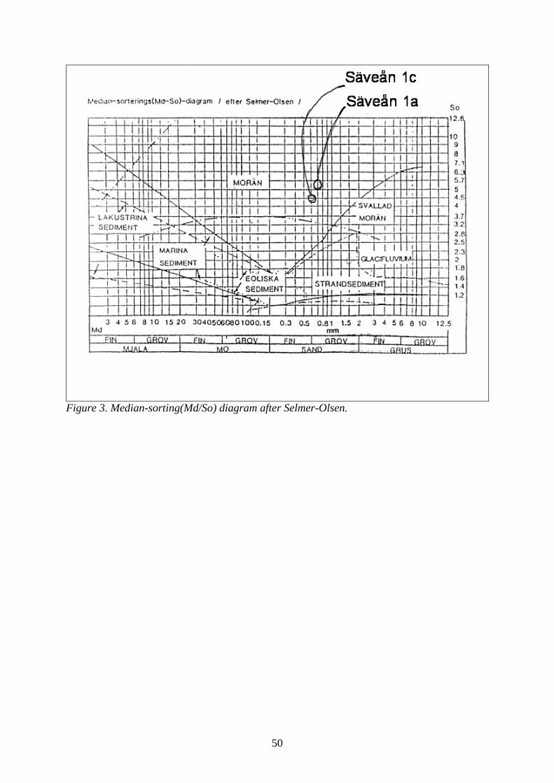
50
Figure 3. Median-sorting(Md/So) diagram after Selmer-Olsen.