University of Groningen Essays on socio-economic

University of Groningen

Essays on socio-economic development in IndiaPieters, Janneke

IMPORTANT NOTE: You are advised to consult the publisher's version (publisher's PDF) if you wish to cite fromit. Please check the document version below.

Document VersionPublisher's PDF, also known as Version of record

Publication date:2011

Link to publication in University of Groningen/UMCG research database

Citation for published version (APA):Pieters, J. (2011). Essays on socio-economic development in India. University of Groningen, SOM researchschool.

CopyrightOther than for strictly personal use, it is not permitted to download or to forward/distribute the text or part of it without the consent of theauthor(s) and/or copyright holder(s), unless the work is under an open content license (like Creative Commons).

The publication may also be distributed here under the terms of Article 25fa of the Dutch Copyright Act, indicated by the “Taverne” license.More information can be found on the University of Groningen website: https://www.rug.nl/library/open-access/self-archiving-pure/taverne-amendment.

Take-down policyIf you believe that this document breaches copyright please contact us providing details, and we will remove access to the work immediatelyand investigate your claim.

Downloaded from the University of Groningen/UMCG research database (Pure): http://www.rug.nl/research/portal. For technical reasons thenumber of authors shown on this cover page is limited to 10 maximum.

Download date: 03-12-2021

https://research.rug.nl/en/publications/essays-on-socioeconomic-development-in-india(4593e871-63f3-48bc-9204-2273f57dc5c5).html

Chapter 4

Push or pull? Drivers of female labor force

participation during India’s economic boom*

4.1 Introduction

India’s economic growth has rapidly increased over the past two decades and future

predictions are optimistic. Female labor force participation was stagnant for a long time,

but started to rise at the turn of the century. Given the positive effect female participation

can have on economic growth (Esteve-Volart, 2004; Klasen and Lamanna, 2009), drawing

women into the labor force can be a significant source of future growth of the Indian

economy. This is particularly the case as higher female participation would be an important

component of the so-called demographic dividend. India currently has an advantageous age

structure of the population with a growing share of working age people and relatively few

dependents (a result of prior fertility decline). Such a demographic dividend, including

higher female participation rates, is alleged to have accounted for about a third of East

Asia’s high per capita growth rates in the period between 1965 and 1990 (Bloom and

Williamson, 1998), but hinges on the productive employment of the working age

population.

Beyond economic benefits, women’s participation in the labor force can be seen as a

signal of declining discrimination and increasing empowerment of women (Mammen and

Paxson, 2000). However, feminization of the workforce is not necessarily a sign of

improvement of women’s opportunities and position in society. It can also be a response to

recession or increasing insecurity in the labor market, with female labor supply functioning

essentially as an insurance mechanism for households (Standing, 1999; Bhalotra and

Umaña-Aponte, 2010). The aim of this chapter is to determine what drives the labor force

participation of women in India. Understanding these determinants is necessary to be able

to understand the implications for women’s wellbeing and for future growth of the labor

force and the economy.

We analyze the period 1983-2005 and focus on the urban sector, which is where most

structural change is taking place.18 To the best of our knowledge, this is the first study of * This chapter is based on an unpublished paper jointly written with Stephan Klasen.

Chapter 4

60

female labor force participation in India that includes unit level data for the year 2004-05

and systematically analyses possible explanations offered in the literature. Furthermore, we

pay special attention to the differences between poorly and highly educated women, which

appears as a highly relevant distinction in the context of India’s economic development

and female participation rates.

Table 1 summarizes the urban female employment figures for the period 1983-2005.

The increase in female labor force participation rate in the period 1999 to 2004, from 21 to

24 per cent, came about after stagnation between 1983 and 1999. In absolute terms, more

than five million women entered the urban labor force in the last period, in particular self-

employed and regular workers.19

Table 1 - Urban female population by employment status (age group 20-59) 1983 1987-88 1993-94 1999-2000 2004-05Self-employed 2,649 (7) 3,249 (7) 3,948 (7) 4,745 (7) 6,675 (8)Regular 2,641 (7) 3,347 (8) 4,311 (8) 5,364 (8) 7,651(10)Casual 2,193 (6) 2,225 (5) 3,000 (5) 2,968 (4) 2,953 (4)Unemployed 530 (1) 785 (2) 976 (2) 909 (1) 1,729 (2)Labor force 8,013 (22) 9,605 (22) 12,235 (22) 13,985 (21) 19,007 (24)Out of labor force 29,034 (78) 34,715 (78) 43,537 (78) 53,308 (79) 61,016(76)Total 37,047(100) 44,325(100) 55,766(100) 67,300(100) 80,031(100)

Note: totals may not add up due to rounding. Numbers are in ‘000s, percentage of total women in this age group in parentheses. Self-employed includes unpaid family workers, but excludes domestic duties. Regular employees receive salary or wages on a regular basis. Casual workers receive a wage according to the terms of the daily or periodic work contract. Source: NSS Employment and Unemployment Survey and Sundaram (2007).

Recent trends in the structure of employment and real earnings suggest that for poorly

educated women, labor force participation is driven by necessity rather than opportunities.

The share of working women in agriculture and manufacturing self-employment and in

domestic services increased, which are often poorly paying and highly insecure jobs.

Furthermore, between 1999 and 2004 real earnings for men and women declined. Highly

educated women are more likely to work in better paying and more attractive jobs in the

services sector, and at the very top real earnings have continued to increase.

18 This focus is also driven by availability and reliability of data on female employment. More than half of rural working women are self-employed, and changes in rural participation rates are driven by the self-employed. Earnings data are not available for the self-employed, which makes it difficult to analyse the determinants of participation in rural India. 19 Part of the increase in the absolute number of working women reflects the share of women aged 20-59 in the total female population, which has risen from 46 to 54 per cent since 1983. Clearly, demographic changes have also contributed to workforce growth, augmenting the recent jump in participation rates.

Push or pull? Drivers of female labor force participation during India’s economic boom

61

A unit level analysis based on the national employment survey sheds further light on the

determinants of participation in paid employment. Our results show that women’s decision

to work is negatively related to the income and employment of household members. An

important finding is that only highly educated women are attracted to the labor market by

higher expected earnings; for women with less than secondary education we find no effect

of market wages on participation in paid employment. This suggests that economic pull

factors reflected in earnings opportunities only attract the highly educated minority of

urban women into the labor force. Furthermore, own education and education of the

household head have a strong negative effect on participation of poorly educated women,

suggesting that income and status effects as well as possibly the lack of white collar job

opportunities are powerful deterrents to female employment in this group.

The rest of this chapter is organized as follows: Section 4.2 summarizes related

literature on development and women’s lab our force participation. Section 4.3 discusses

previous research on India, and describes in more detail the trends in employment and

earnings in India during the recent past. Section 4.4 presents an empirical model and

estimation results for women’s participation in paid employment. Finally, section 4.5

summarizes the main findings and conclusions.

4.2 Determinants of female labor force participation

The basic static labor supply model is a starting point for many models of female labor

force participation (see Blundell and MaCurdy, 1999). In this model, an increase in the

wage rate reduces demand for leisure as its opportunity cost rises, and labor supply will

increase. If leisure is a normal good, an increase in a person’s or their household members’

income will increase the demand for leisure and thus reduce her hours worked. These are

the well-known substitution and income effects. For a person with positive labor supply

(i.e., who currently works for pay), the overall net effect on labor supply of an increase in

the wage rate depends on the relative strength of the substitution and income effect, and is

theoretically ambivalent. For a person currently not working, an increase in the wage rate

only has a substitution effect, increasing the incentive to work. An increase in unearned

income (income earned by other household members) reduces labor supply through the

negative income effect.

Chapter 4

62

4.2.1 Development and women’s participation

Beyond the basic labor supply model, several further factors have been discussed in the

analysis of female labor force participation in developing countries. Probably the best-

known hypothesis in this literature is the feminization U-curve, which suggests that female

labor force participation first declines and then increases as an economy develops (Goldin,

1994; Mammen and Paxson, 2000). The U-curve is the outcome of a combination of

structural change in the economy, income effects, and social stigma against factory work

by women. In initial stages of development, education levels rise and employment shifts

from agriculture to manufacturing. But in these initial stages, education increases much

more for men than for women. Unearned income rises fast while women’s wages and

opportunities for work change relatively slowly, so the positive substitution effect of rising

female wages is likely to be dominated by a negative income effect. Participation is further

reduced because of social stigma against women working in manufacturing. Later on,

women’s education rises as well, while demand for white-collar workers increases with the

expansion of the services sector. Higher wages and socially acceptable types of work lead

to higher female labor force participation. Though the feminization U is sometimes

considered a stylized fact, the empirical evidence in support of it is mostly based on cross-

country analysis, while panel analyses have produced mixed results (e.g., Çagatay and

Özler, 1995; Tam, 2011; Gaddis and Klasen, 2011).

One might well hypothesize that within a country, there is a U-shape relationship

between economic or educational status and women’s labor force participation at a given

point in time. Among the poorly educated, women are forced to work to survive and can

combine farm work with domestic duties, and among the very highly educated, high wages

induce women to work and stigmas militating against female employment may be low.

Between these two groups, women may face barriers to labor force participation related to

both the absence of an urgent need of female employment, and the presence of social

stigmas associated with female employment.20 This would be consistent with a similar U-

shape relationship in gender bias in mortality by education or income groups, where gender

bias appears to be largest among the middle groups (e.g. Klasen and Wink, 2003; Drèze

and Sen, 2002). In any case, the feminization U hypothesis (at the country or international

20

Attitudes of both men and women towards gender roles can be shaped by factors such as religion (Lehrer, 1995; Amin and Alam, 2008), education, mass communication, and attitudes and behaviour of previous generations (e.g., Farré and Vella, 2007).


63

level) reflects several underlying forces at work, and we aim to unravel these using

disaggregated analysis.

Female participation rates may also be determined by the level of employment security.

Standing (1999) argues that growing labor market flexibility and diverse forms of

insecurity have encouraged greater female labor force participation around the world.

Technological change and increasing international competition stimulate employers to

focus on a limited number of permanent core workers, while making more use of

temporary workers and subcontracting. Women are often more prepared to engage in more

flexible, short-term, informal types of employment and as a result relative demand for

women increases. And through reduction in social security and more income insecurity

women are pushed into the labor market. Rising female labor force participation then

reflects the erosion of men’s position in the labor market, rather than an improvement in

women’s opportunities.

This view is related to the view of women’s labor supply as an insurance mechanism for

households (Attanasio et al., 2005). In a recent paper, Bhalotra and Umaña-Aponte (2010)

show that in developing countries in Asia and Latin America, female labor force

participation rates move counter-cyclically: women move from non-employment into paid

and self-employment during recessions. In line with the insurance mechanism theory, they

also find that counter-cyclicality is strongest in households with limited alternative sources

of insurance against income shocks.

The role of women as caregivers and their high domestic work burden are obviously

also important when it comes to the participation decision, as this determines their value

within the household. Cunningham (2001) shows that in Mexico, unmarried women

without children are as likely to work as men, while labor supply of married women

depends on the presence of young children and the level and stability of household income.

With declining fertility, the value of nonworking time declines and one would expect

female labor force participation rates to rise.21

The different views discussed here are not mutually exclusive, and can be summarized

in terms of the following hypotheses about determinants of women’s participation:

- The woman’s expected market wage positively affects participation.

21 This need not necessarily be the case, however. As shown by Priebe (2011) in the case of Indonesia, declining fertility might actually reduce female labor force participation rates among poorer parts of the population where fertility decline reduces the need to work.

Chapter 4

64

- Unearned income, including income from non-labor sources and other household

members has a negative effect on participation;

- Income and employment insecurity of other household members induces higher

participation;

- Social stigma, possibly related to (own or husband’s) education and the type of work (at

home or outside, manual or non-manual work), negatively affect female employment;

- Large family size and a high household workload have negative effects.

All of these, except the expected market wage, are determinants of the so-called

reservation wage, which can be thought of as the marginal utility of non-work (including

childcare and housework): when the expected market wage exceeds the reservation wage, a

woman will participate in the labor force. This set-up will be used in the individual-level

empirical analysis in section 4.4.

4.3 Women’s participation in India

There has not been very much research on female labor force participation in India, but

it is generally known that the participation rate is low compared to other countries. In 1998

India’s Central Statistical Organization conducted a time use survey in six states, for which

household duties (household maintenance and care for children, old, and sick household

members) were classified as “extended-SNA” activities. Time spent on SNA activities,

which are economic activities included in the national accounts, was measured separately.

The survey showed that urban women spent about nine hours per week on SNA activities

plus 36 hours on extended-SNA activities, against 41plus three hours weekly, respectively,

for men (NCEUS, 2007). Mitra (2005) names the dual burden of conventional productive

work and household duties as one of the major constraints to women’s labor market

choice: male household members typically decide on the location of residence, and women

depend on informal networks to find paid employment near their homes.

Besides the double burden of work, social norms restrict women’s availability and

location of work leading to lower labor force participation (NCEUS, 2007).This may be

reflected in the clear U-shaped relationship between women’s education and labor force

participation in India. Kingdon and Unni (2001) attribute the downward sloping part of this

U to the process of Sanskritization: social restrictions on the lifestyles of women tend to

become more rigid as households move up in the caste hierarchy (Chen and Drèze, 1992),

which would be reinforced by the negative income effect of rising incomes of husbands.

Increasing participation at the highest education levels could reflect modernizing


65

influences that increase women’s aspirations, combined with higher returns to education

that increase economic incentives for women to work. Bardhan (1986) argues that class,

patriarchy, and social hierarchy (caste, ethnicity, and religion) all interact to shape attitudes

towards gender roles. In that sense, the downward sloping part of the U reflects not just

Sanskritization, but a general aspiration to upgrade social status or imitate lifestyles of

higher status groups. Among higher classes, aspired status groups would be the urban

educated with more Western lifestyles, associated with higher female labor force

participation rates.

Analyzing regional differences in female participation rates in the 1990s, Ahasan and

Pages (2008) find that employment opportunities play an important role especially in rural

India, as female wages or expected earnings have a strong positive effect on participation.

They also find some evidence for a negative income effect of men’s earnings. Besides

these classical income and substitution effects, however, the impact of cultural and social

factors is not considered in their analysis. Based on a survey among 447 households in

Delhi in 2006, Sudarshan and Bhattacharya (2009) find that besides women’s household

workload, lack of information and mobility and safety concerns are important constraints

to her participation. The decision to work is mainly determined by the external

environment (e.g., child care arrangements and safety in public spaces) and ideology of the

marital household, rather than the woman’s individual attributes.

Regarding the recent increase in participation rates, there is some evidence for rural

India that women’s labor market entry between 1999 and 2004 was distress-driven: self-

employment increased most among the poorest households, real wage growth stagnated,

and the workforce feminization was greatest in the farm sector in districts with agricultural

distress (Abraham, 2009). The story for urban India may be less gloomy, as job

opportunities are likely to be quite different: especially services sector employment is

concentrated in urban India. The next section gives a more detailed description of changes

in the Indian urban labor market over the past decades.

4.3.1 Trends in employment and earnings in urban India

Data on employment and earnings used in this chapter are from the four most recent

‘thick’ rounds of the National Sample Survey (NSS) on Employment and Unemployment,

Chapter 4

66

the official source of employment and earnings data used by the Government of India.

They are for the years 1987-88, 1993-94, 1999-00, and 2004-5.22

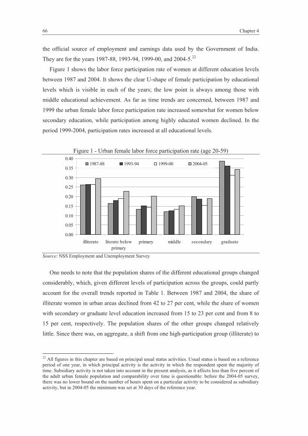
Figure 1 shows the labor force participation rate of women at different education levels

between 1987 and 2004. It shows the clear U-shape of female participation by educational

levels which is visible in each of the years; the low point is always among those with

middle educational achievement. As far as time trends are concerned, between 1987 and

1999 the urban female labor force participation rate increased somewhat for women below

secondary education, while participation among highly educated women declined. In the

period 1999-2004, participation rates increased at all educational levels.

Figure 1 - Urban female labor force participation rate (age 20-59)

0.00

0.05

0.10

0.15

0.20

0.25

0.30

0.35

0.40

illiterate literate belowprimary

primary middle secondary graduate

1987-88 1993-94 1999-00 2004-05

Source: NSS Employment and Unemployment Survey

One needs to note that the population shares of the different educational groups changed

considerably, which, given different levels of participation across the groups, could partly

account for the overall trends reported in Table 1. Between 1987 and 2004, the share of

illiterate women in urban areas declined from 42 to 27 per cent, while the share of women

with secondary or graduate level education increased from 15 to 23 per cent and from 8 to

15 per cent, respectively. The population shares of the other groups changed relatively

little. Since there was, on aggregate, a shift from one high-participation group (illiterate) to

22 All figures in this chapter are based on principal usual status activities. Usual status is based on a reference period of one year, in which principal activity is the activity in which the respondent spent the majority of time. Subsidiary activity is not taken into account in the present analysis, as it affects less than five percent of the adult urban female population and comparability over time is questionable: before the 2004-05 survey, there was no lower bound on the number of hours spent on a particular activity to be considered as subsidiary activity, but in 2004-05 the minimum was set at 30 days of the reference year.


67

two other high-participation groups (secondary and graduate), these population shifts

hardly affected the overall female participation rate.

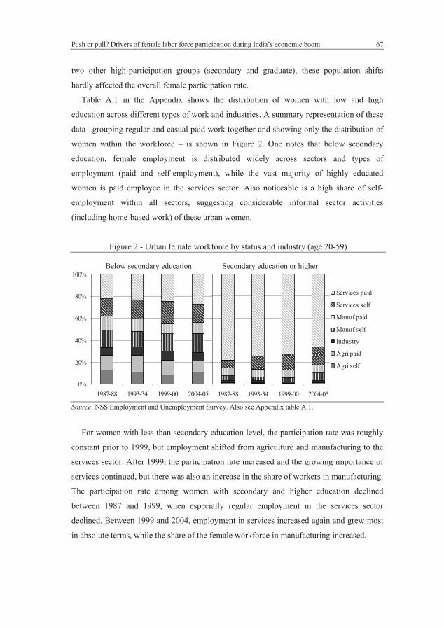
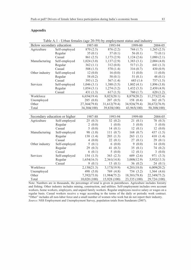
Table A.1 in the Appendix shows the distribution of women with low and high

education across different types of work and industries. A summary representation of these

data –grouping regular and casual paid work together and showing only the distribution of

women within the workforce – is shown in Figure 2. One notes that below secondary

education, female employment is distributed widely across sectors and types of

employment (paid and self-employment), while the vast majority of highly educated

women is paid employee in the services sector. Also noticeable is a high share of self-

employment within all sectors, suggesting considerable informal sector activities

(including home-based work) of these urban women.

Figure 2 - Urban female workforce by status and industry (age 20-59)

Below secondary education Secondary education or higher

0%

20%

40%

60%

80%

100%

1987-88 1993-34 1999-00 2004-05 1987-88 1993-34 1999-00 2004-05

Services paid

Services self

Manuf paid

Manuf self

Industry

Agri paid

Agri self

Source: NSS Employment and Unemployment Survey. Also see Appendix table A.1.

For women with less than secondary education level, the participation rate was roughly

constant prior to 1999, but employment shifted from agriculture and manufacturing to the

services sector. After 1999, the participation rate increased and the growing importance of

services continued, but there was also an increase in the share of workers in manufacturing.

The participation rate among women with secondary and higher education declined

between 1987 and 1999, when especially regular employment in the services sector

declined. Between 1999 and 2004, employment in services increased again and grew most

in absolute terms, while the share of the female workforce in manufacturing increased.

Chapter 4

68

A closer look at the growth of female employment in manufacturing and services

reveals some interesting patterns. First, the rising share of women in manufacturing after

1999 (at all educational levels) is driven by an increase in self-employment in this sector,

which is very much concentrated in the wearing apparel industry. According to a study of

the industry in Tiruppur, a city in South India, and in Delhi, the boom in garment exports

in the 1990s attracted many women, who remain concentrated in the lowest paying

activities and occupy a highly invisible part of the value chain as home-based workers.

Home-based workers receive piece-rate payment and constitute an important buffer for

demand fluctuations, thus facing huge income variations (Singh and Sapra, 2007). This

description of workforce informalization is in line with Standing (1999), who argues it

pushes rather than pulls women into the labor force.

Among the poorly educated women with regular paid employment in the services

sector, the share working in private households (maids, cooks, etc.) increased from 44 to

62 per cent between 1999 and 2004. That is, almost one million women joined the labor

force as domestic servants, which is a group of legally and socially vulnerable workers.

They are not covered by existing legislation and are easy victims of exploitation due to

their invisibility, lack of education and, often, migration background (Ramirez-Machado,

2003; NCEUS, 2007).

Among the highly educated women in the services sector, the share in public

administration declined from 16 to 11 per cent during 1999-2004, while the share of both

domestic servants and software consultants increased from less than half percent to over

two per cent each. Among the highly educated self-employed women in services, the share

in retail declined from 31 to 18 per cent, while the largest increases were in ‘adult and

other education’ (15 to 20 per cent) and ‘other services’ (7 to 11 per cent).

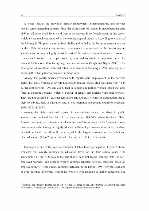
Earnings are one of the key determinants of labor force participation. Figure 3 shows

women’s real weekly earnings by education level for the four survey years. One

shortcoming of the NSS data is the fact that it does not record earnings data for self-

employed workers. The average weekly earnings reported here are therefore based on

employees only.23 Real weekly earnings increased in the period 1993-1999 but stagnated

or even declined afterwards, except for workers with graduate or higher education. The

23 Earnings are spatially deflated and in 1987-88 Rupees, based on the Labor Bureau Consumer Price Index for Industrial Workers and Deaton (2003). No adjustment is made for hours worked.


69

level of earnings is substantially higher for men (not shown), but the pattern of change is

similar.

Figure 3 - Average real weekly earnings (in Rs.) for urban females age 20-59

0

100

200

300

400

500

1987-88 1993-94 1999-00 2004-05

graduate

secondary

middle

primary

literate

illiterate

Source: NSS Employment and Unemployment Survey

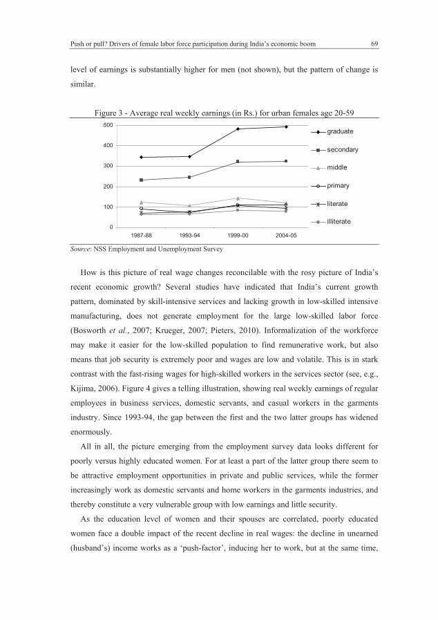
How is this picture of real wage changes reconcilable with the rosy picture of India’s

recent economic growth? Several studies have indicated that India’s current growth

pattern, dominated by skill-intensive services and lacking growth in low-skilled intensive

manufacturing, does not generate employment for the large low-skilled labor force

(Bosworth et al., 2007; Krueger, 2007; Pieters, 2010). Informalization of the workforce

may make it easier for the low-skilled population to find remunerative work, but also

means that job security is extremely poor and wages are low and volatile. This is in stark

contrast with the fast-rising wages for high-skilled workers in the services sector (see, e.g.,

Kijima, 2006). Figure 4 gives a telling illustration, showing real weekly earnings of regular

employees in business services, domestic servants, and casual workers in the garments

industry. Since 1993-94, the gap between the first and the two latter groups has widened

enormously.

All in all, the picture emerging from the employment survey data looks different for

poorly versus highly educated women. For at least a part of the latter group there seem to

be attractive employment opportunities in private and public services, while the former

increasingly work as domestic servants and home workers in the garments industries, and

thereby constitute a very vulnerable group with low earnings and little security.

As the education level of women and their spouses are correlated, poorly educated

women face a double impact of the recent decline in real wages: the decline in unearned

(husband’s) income works as a ‘push-factor’, inducing her to work, but at the same time,

Chapter 4

70

the decline in her own market wage would reduce her incentive to work. With the recent

rise in participation rates, it seems that push-factors dominate the decision of lowly

educated women to work. On the other hand, more attractive employment opportunities

exist for highly educated women, who have higher earnings potential and increasing

earnings at the very top, and are less likely to face declining unearned income of partners.

This will be analyzed more formally in the next section.

Figure 4 - Average real weekly earnings selected industries, urban females (20-59)

0

100

200

300

400

500

600

1987-88 1993-94 1999-00 2004-05

business services (regular) domestic servants garments (casual)

Note: real weekly earnings in 1987-88 Rupees. Source: NSS Employment and Unemployment Survey

4.4 Empirical model and estimation results

In light of the employment structure and changes in real earnings for different levels of

education and in different industries, the main question is to what extent participation of

women is affected by negative income effects, positive own wage effects, and some sort of

insurance mechanism to cope with increasing insecurity in the labor market. We

hypothesize that poorly educated women’s participation is largely driven by income and

insurance considerations, whereas highly educated women respond more to opportunities

reflected in market wages. To test this, we use unit-level data to analyze the determinants

of labor force participation separately for women with low and high education.

4.4.1 Probability of women’s participation

We analyze women’s participation decision at the individual level, based on a sample of

urban women aged 20 to 59, excluding women who are enrolled in education or unable to


71

work due to disability, and women who are head of their household.24 Self-employed

women are dropped from the sample due to the non-availability of self-employment

earnings data: the expected market wage can only be estimated for employees. We do

check the robustness of results with respect to this restriction of the sample in section 4.3.

The probability Pit of woman i in year t being employed is estimated using a binary

probit model, which is estimated separately for each year, for women below secondary

education and for women with secondary or higher education.

ittittrtit ZwFp ˆln , (1)

where F is the standard normal cumulative distribution function. The model includes a

region fixed effect αrt, which controls for regional level participation determinants such as

the region’s sectoral structure.25 Other regressors are the log expected market wage itwln ,

and a vector Zit consisting of:

- Unearned income per capita (other household members’ real weekly earnings, divided

by household size)

- Security of unearned income (the share of unearned income earned through regular

employment)

- Underemployment of male adult household members (whether male household

members were without work for one or more months during the reference year)

- Marital status

- The number of children in the household by age group (0-4 and 5-14 years old)

- Social group (whether a person belongs to a scheduled caste or tribe, SCST)

- Religion

- Own education level and education level of the household head

Since wages are observed only for employed women, we need to impute wages for those

not employed. To this end, we estimate a standard wage equation with Heckman selection

bias correction (Heckman, 1979). Real weekly earnings are regressed on age, its square,

and education level, controlling for sample selection:

itittjitjtittitttit ubEdubAgebAgebbw 432

210ln , (2)

24 About six per cent of women in the sample (roughly 2,500 observations in each survey round) is head of her household. They are excluded because we want to estimate the effect of women’s own education separately from household head’s education, which proxies for household wealth and status effects. 25 In India, the region is one administrative level below the state and is comprised of multiple districts. The sample contains 61 regions.

Chapter 4

72

where wi is real weekly earnings, Eduji is a vector of dummy variables for education level,

and i is the sample selection correction term. The latter is obtained (as the inverse Mills

ratio, or the ratio of the probability density function over the cumulative distribution

function) from a probit model for participation. This selection equation is equal to equation

(1), except that the expected market wage is replaced by age and age squared:

ittittittrtit ZcAgebAgebaFp 221 . (3)

The wage model (equations 2 and 3) is identified on the variables in Zit, except for

education, which is included in both the wage equation and the selection equation.

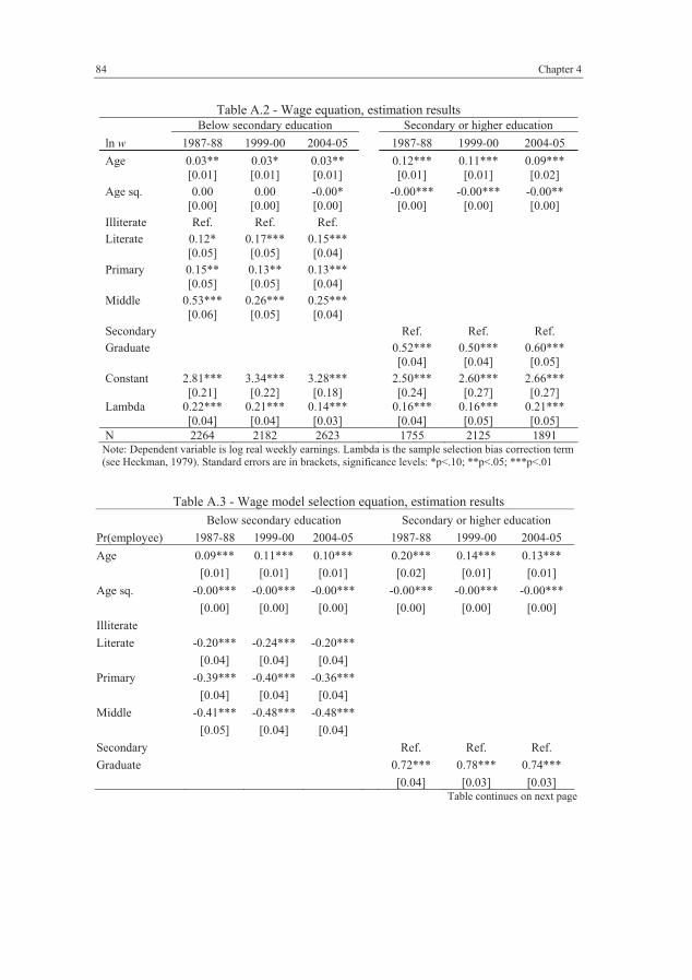
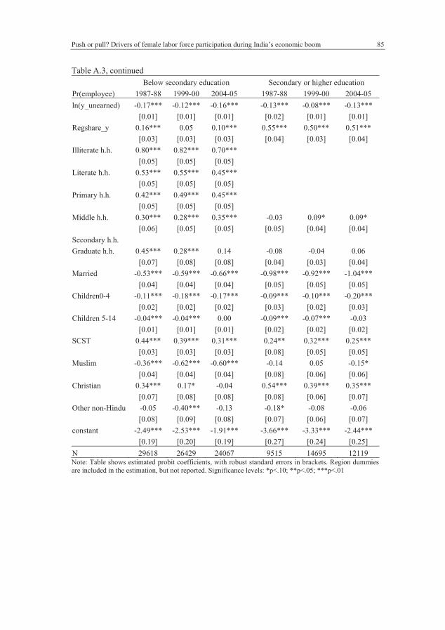
Estimation results are shown in Appendix table A.2, for the wage equation, and A.3, for

the selection equation. The expected market wage itwln used in the estimation of equation

(1) is then the fitted value of the wage using the parameter estimates of equation (2)

(without the sample selection term).

Implicit in the empirical model is the assumption that women’s participation decision is

made conditional on men’s, so we do not consider joint utility maximization or bargaining

within the household. Furthermore, some of the covariates are likely to be endogenous in

the sense that there might be underlying factors simultaneously affecting the covariates and

the dependent variable. This might particularly be the case for marital status and number of

children. We would plausibly assume that such endogeneity would bias the coefficients on

marital status and children downwards (as the marriage decision and the decision to have

children might be jointly determined with the decision not to work). When interpreting the

coefficients, these potential biases should be kept in mind.26

The explanatory variables in the participation model of equation (1) are all measured

using the NSS survey data, but some of these are not directly observable. To measure

unearned income (y_unearned), the earnings of self-employed household members are

imputed based on the earnings of employees. It appears this imputation serves the purpose

of measuring unearned income per capita reasonably well as the results are very similar

when households with one or more self-employed adults are excluded from the samples. In

the final estimation, we therefore rely on the imputed earnings in order to retain as many

observations as possible.

26 Own education might also be jointly determined with the labor force participation decision. But since we control for the own wage, education is included precisely as a proxy for the labor market orientation of the woman, rather her human capital; we are not treating the coefficient of own education as a causal mechanism of human capital, but as an indicator of work orientation.


73

As a proxy for income security, we include the share of unearned income that is earned

through regular employment (Regshare_y). This is based on the notion that regular

employment provides more stable and secure income than other types of work.

Additionally, in the surveys for 1999-2000 and 2004-05, working persons report for how

many months during the reference year they were without work. This is used to measure

underemployment, as an indicator variable which is equal to one if at least one working

male household member reports one or more months without work.27

Marital status and the number of children are included to capture family obligations

which are likely to negatively affect female labor force participation (as noted above, there

might be endogeneity issues here). Social group and religion are proxies for attitudes

towards women’s work. Members of a scheduled caste or tribe (SCST) are expected to be

more likely to work, as these are the lowest social classes in India, in which there is no

economic room to withdraw women from the labor force and to emulate higher classes

(Bardhan, 1986). Religiosity in general has been related to more traditional views of

women’s role (Jaeger, 2010; Seguino, 2011); previous studies have found that Muslim

women in India have lower participation rates than women of other religions (Das and

Desai, 2003). We therefore include dummy variables indicating whether the woman is

Hindu (the reference category), Muslim, Christian, or of another/no religion.

Finally, we control for own education level and the household head’s education level.

Household head education captures the socio-economic status of the household, but also

proxies for household wealth (in addition to unearned income, which includes only current

weekly earnings of household members). If higher status leads to more restrictions on

women and higher wealth reduces the need for women to work, the education level of the

head should have a strong negative effect on participation, except for the very top:

graduates may have more ‘modern’ attitudes towards women’s work. Own education is

included as an indicator of work orientation and to capture non-wage compensation for

work (see Blau and Kahn, 2007), so one would expect a positive effect of own education

on participation. However, since there is a strong (unconditional) U-shaped relationship

between women’s education and participation in India (see Figure 1), it might well be the

case that own education has a negative effect on participation in the low-education sample

(women with primary or middle school level work less than illiterates). Since the U-shape

has been ascribed to changing attitudes related to household status, combined with effects

27 Data on this subject in 1987-88 are not comparable with the more recent survey rounds.

Chapter 4

74

of unearned income and women’s own earnings potential, it remains an empirical question

whether the effect of own education is still U-shaped after separately controlling for own

wage, unearned income, household head education, and other covariates.

Table 2 - Average values, low education sample 1987-88 1999-00 2004-05

mean st.dev. mean st.dev. mean st.dev.

Employee 0.09 0.29 0.09 0.29 0.12 0.33ln(ŵ) 3.70 0.21 4.00 0.12 4.03 0.12ln(y_unearned) 3.48 1.06 3.73 1.16 3.69 1.12Regshare_y 0.41 0.47 0.36 0.45 0.33 0.44Underemployment 0.16 0.37 0.18 0.39Age 35.14 10.81 36.04 10.49 36.23 10.62Illiterate 0.51 0.50 0.45 0.50 0.43 0.49Literate below primary 0.13 0.34 0.13 0.33 0.13 0.33Primary school 0.20 0.40 0.18 0.39 0.19 0.40Middle school 0.16 0.36 0.24 0.43 0.25 0.43Married 0.89 0.31 0.90 0.29 0.90 0.30Children 0-4 0.78 0.98 0.63 0.92 0.63 0.92Children 5-14 1.42 1.40 1.33 1.42 1.23 1.35SCST 0.16 0.37 0.21 0.41 0.23 0.42Hindu 0.74 0.44 0.74 0.44 0.76 0.43Muslim 0.20 0.40 0.21 0.41 0.20 0.40Christian 0.02 0.14 0.02 0.14 0.02 0.13Other religion 0.04 0.19 0.04 0.19 0.03 0.17Illiterate household head 0.26 0.44 0.26 0.44 0.26 0.44Literate below prim h.h. 0.16 0.37 0.14 0.35 0.14 0.35Primary h.h. 0.19 0.40 0.15 0.35 0.17 0.38Middle h.h. 0.16 0.36 0.19 0.39 0.19 0.39Secondary h.h. 0.18 0.38 0.21 0.41 0.19 0.39Graduate h.h. 0.05 0.23 0.06 0.23 0.05 0.21

N 29593 26026 24015 Source: NSS Employment and Unemployment Survey.

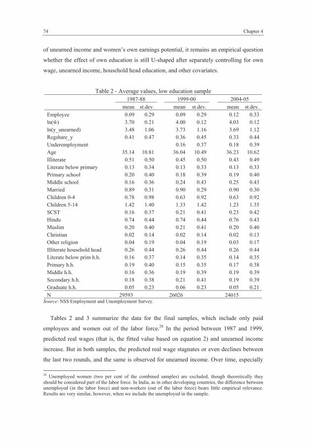
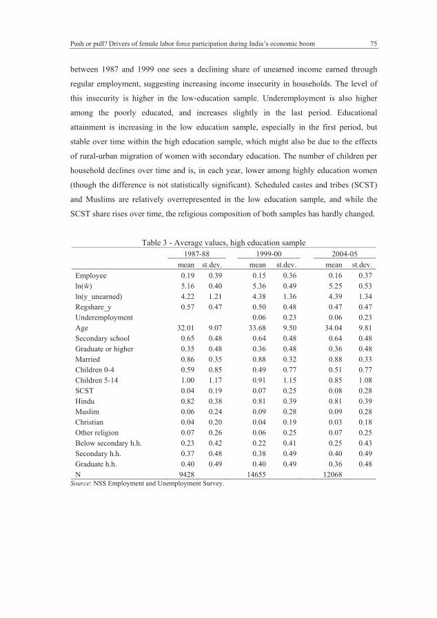
Tables 2 and 3 summarize the data for the final samples, which include only paid

employees and women out of the labor force.28 In the period between 1987 and 1999,

predicted real wages (that is, the fitted value based on equation 2) and unearned income

increase. But in both samples, the predicted real wage stagnates or even declines between

the last two rounds, and the same is observed for unearned income. Over time, especially

28 Unemployed women (two per cent of the combined samples) are excluded, though theoretically they should be considered part of the labor force. In India, as in other developing countries, the difference between unemployed (in the labor force) and non-workers (out of the labor force) bears little empirical relevance. Results are very similar, however, when we include the unemployed in the sample.


75

between 1987 and 1999 one sees a declining share of unearned income earned through

regular employment, suggesting increasing income insecurity in households. The level of

this insecurity is higher in the low-education sample. Underemployment is also higher

among the poorly educated, and increases slightly in the last period. Educational

attainment is increasing in the low education sample, especially in the first period, but

stable over time within the high education sample, which might also be due to the effects

of rural-urban migration of women with secondary education. The number of children per

household declines over time and is, in each year, lower among highly education women

(though the difference is not statistically significant). Scheduled castes and tribes (SCST)

and Muslims are relatively overrepresented in the low education sample, and while the

SCST share rises over time, the religious composition of both samples has hardly changed.

Table 3 - Average values, high education sample 1987-88 1999-00 2004-05

mean st.dev. mean st.dev. mean st.dev.

Employee 0.19 0.39 0.15 0.36 0.16 0.37ln(ŵ) 5.16 0.40 5.36 0.49 5.25 0.53ln(y_unearned) 4.22 1.21 4.38 1.36 4.39 1.34Regshare_y 0.57 0.47 0.50 0.48 0.47 0.47Underemployment 0.06 0.23 0.06 0.23Age 32.01 9.07 33.68 9.50 34.04 9.81Secondary school 0.65 0.48 0.64 0.48 0.64 0.48Graduate or higher 0.35 0.48 0.36 0.48 0.36 0.48Married 0.86 0.35 0.88 0.32 0.88 0.33Children 0-4 0.59 0.85 0.49 0.77 0.51 0.77Children 5-14 1.00 1.17 0.91 1.15 0.85 1.08SCST 0.04 0.19 0.07 0.25 0.08 0.28Hindu 0.82 0.38 0.81 0.39 0.81 0.39Muslim 0.06 0.24 0.09 0.28 0.09 0.28Christian 0.04 0.20 0.04 0.19 0.03 0.18Other religion 0.07 0.26 0.06 0.25 0.07 0.25Below secondary h.h. 0.23 0.42 0.22 0.41 0.25 0.43Secondary h.h. 0.37 0.48 0.38 0.49 0.40 0.49Graduate h.h. 0.40 0.49 0.40 0.49 0.36 0.48N 9428 14655 12068

Source: NSS Employment and Unemployment Survey.

Chapter 4

76

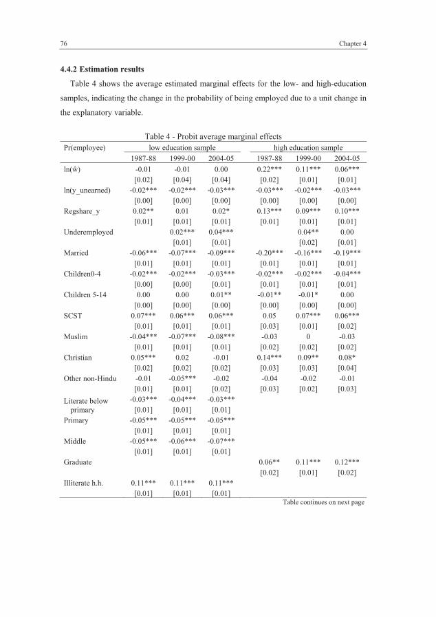
4.4.2 Estimation results

Table 4 shows the average estimated marginal effects for the low- and high-education

samples, indicating the change in the probability of being employed due to a unit change in

the explanatory variable.

Table 4 - Probit average marginal effects

Pr(employee) low education sample high education sample

1987-88 1999-00 2004-05 1987-88 1999-00 2004-05

ln(ŵ) -0.01 -0.01 0.00 0.22*** 0.11*** 0.06*** [0.02] [0.04] [0.04] [0.02] [0.01] [0.01] ln(y_unearned) -0.02*** -0.02*** -0.03*** -0.03*** -0.02*** -0.03*** [0.00] [0.00] [0.00] [0.00] [0.00] [0.00] Regshare_y 0.02** 0.01 0.02* 0.13*** 0.09*** 0.10*** [0.01] [0.01] [0.01] [0.01] [0.01] [0.01] Underemployed 0.02*** 0.04*** 0.04** 0.00 [0.01] [0.01] [0.02] [0.01] Married -0.06*** -0.07*** -0.09*** -0.20*** -0.16*** -0.19*** [0.01] [0.01] [0.01] [0.01] [0.01] [0.01] Children0-4 -0.02*** -0.02*** -0.03*** -0.02*** -0.02*** -0.04*** [0.00] [0.00] [0.01] [0.01] [0.01] [0.01] Children 5-14 0.00 0.00 0.01** -0.01** -0.01* 0.00 [0.00] [0.00] [0.00] [0.00] [0.00] [0.00] SCST 0.07*** 0.06*** 0.06*** 0.05 0.07*** 0.06*** [0.01] [0.01] [0.01] [0.03] [0.01] [0.02] Muslim -0.04*** -0.07*** -0.08*** -0.03 0 -0.03 [0.01] [0.01] [0.01] [0.02] [0.02] [0.02] Christian 0.05*** 0.02 -0.01 0.14*** 0.09** 0.08* [0.02] [0.02] [0.02] [0.03] [0.03] [0.04] Other non-Hindu -0.01 -0.05*** -0.02 -0.04 -0.02 -0.01 [0.01] [0.01] [0.02] [0.03] [0.02] [0.03]

Literate below primary

-0.03*** -0.04*** -0.03*** [0.01] [0.01] [0.01]

Primary -0.05*** -0.05*** -0.05*** [0.01] [0.01] [0.01] Middle -0.05*** -0.06*** -0.07*** [0.01] [0.01] [0.01] Graduate 0.06** 0.11*** 0.12*** [0.02] [0.01] [0.02] Illiterate h.h. 0.11*** 0.11*** 0.11*** [0.01] [0.01] [0.01]

Table continues on next page


77

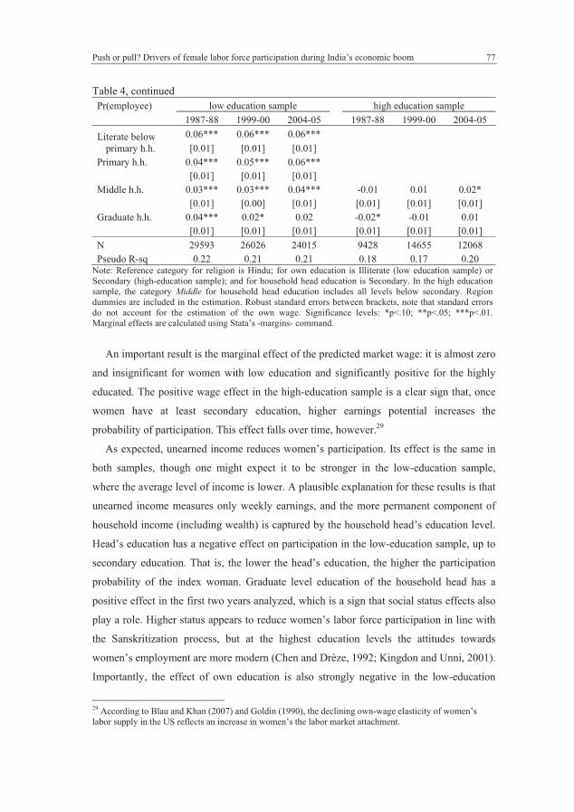
Table 4, continued

Pr(employee) low education sample high education sample

1987-88 1999-00 2004-05 1987-88 1999-00 2004-05

Literate below primary h.h.

0.06*** 0.06*** 0.06***

[0.01] [0.01] [0.01] Primary h.h. 0.04*** 0.05*** 0.06*** [0.01] [0.01] [0.01] Middle h.h. 0.03*** 0.03*** 0.04*** -0.01 0.01 0.02* [0.01] [0.00] [0.01] [0.01] [0.01] [0.01] Graduate h.h. 0.04*** 0.02* 0.02 -0.02* -0.01 0.01 [0.01] [0.01] [0.01] [0.01] [0.01] [0.01]

N 29593 26026 24015 9428 14655 12068 Pseudo R-sq 0.22 0.21 0.21 0.18 0.17 0.20

Note: Reference category for religion is Hindu; for own education is Illiterate (low education sample) or Secondary (high-education sample); and for household head education is Secondary. In the high education sample, the category Middle for household head education includes all levels below secondary. Region dummies are included in the estimation. Robust standard errors between brackets, note that standard errors do not account for the estimation of the own wage. Significance levels: *p<.10; **p<.05; ***p<.01. Marginal effects are calculated using Stata’s -margins- command.

An important result is the marginal effect of the predicted market wage: it is almost zero

and insignificant for women with low education and significantly positive for the highly

educated. The positive wage effect in the high-education sample is a clear sign that, once

women have at least secondary education, higher earnings potential increases the

probability of participation. This effect falls over time, however.29

As expected, unearned income reduces women’s participation. Its effect is the same in

both samples, though one might expect it to be stronger in the low-education sample,

where the average level of income is lower. A plausible explanation for these results is that

unearned income measures only weekly earnings, and the more permanent component of

household income (including wealth) is captured by the household head’s education level.

Head’s education has a negative effect on participation in the low-education sample, up to

secondary education. That is, the lower the head’s education, the higher the participation

probability of the index woman. Graduate level education of the household head has a

positive effect in the first two years analyzed, which is a sign that social status effects also

play a role. Higher status appears to reduce women’s labor force participation in line with

the Sanskritization process, but at the highest education levels the attitudes towards

women’s employment are more modern (Chen and Drèze, 1992; Kingdon and Unni, 2001).

Importantly, the effect of own education is also strongly negative in the low-education

29 According to Blau and Khan (2007) and Goldin (1990), the declining own-wage elasticity of women’s labor supply in the US reflects an increase in women’s the labor market attachment.

Chapter 4

78

sample: the downward sloping part of the U-shaped relationship between education and

participation remains after controlling for own wages, unearned income, and household

head education. Note that if one presumed endogeneity issues here, one would expect that

the coefficients on own education are biased upwards; thus this central finding is unlikely

to be affected by endogeneity. One explanation for this persistent negative effect of own

education is suggested by Das and Desai (2003), who argue that women have a stronger

preference for white collar jobs as their education increases, and participation declines

because these types of jobs are very scarce. But it may also be a status effect of the

Sanskritization process that is captured by own education and not only the household

head’s.

In the high-education sample there is no clear effect of household head education, while

the own education level has a positive effect on participation. Together with the own-wage

effects, these results point out that highly educated women, in contrast to the poorly

educated, are pulled into the workforce by greater earnings opportunities and their

education increases work orientation or aspirations. This is in line with the more standard

models of labor supply and just like the decline of the own wage effect over time, the

rising effect of own education corresponds to rising labor force attachment of women with

graduate level education. Moreover, with India’ booming high-skilled services (like

software consultancy), graduate level education is likely to open up very attractive, non-

manual, employment opportunities for women.

Turning to employment and income insecurity, we find that participation increases with

the share of unearned income from regular employment, especially among highly educated

women. This contrasts with the idea that women are less likely to work if their unearned

income is more secure. A possible explanation is that we capture whether or not any of the

woman’s household members have regular employment, which could provide the

necessary network or information for women to find paid employment themselves. It could

also reduce entry barriers to paid employment through familiarity with employers,

reducing families’ safety concerns (Sudarshan and Bhattacharya, 2009).

Underemployment of male household members, an alternative proxy for insecurity

facing the household, does increase the probability of women’s participation: for a given

level of unearned income, if a male household member is without work for at least one

month of the year, a woman is two to four percentage points more likely to work. The

effect is strongest, and slightly increasing over time, in the low-education sample.


79

The household composition effects show that unmarried women are more likely to

work, especially among highly educated women. Having young children reduces

participation in both samples, while older children have only a very small negative effect

in the high-education sample: possibly, only highly educated women can afford to stay at

home with older children, but the effect of older children disappears in 2004-05. As

endogeneity is likely to be an issue, the effects of marriage and children may be biased

downwards and one should be careful to interpret these effects as causal.

Women belonging to a Scheduled Caste or Tribe are more likely to work for pay, and

religion matters in both samples, but to different degrees. Muslim women are less likely to

work, which is in line with previous studies (e.g., Das and Desai, 2003) but we clearly see

that education mitigates the difference between Muslim and non-Muslim women. Christian

women are more likely to work especially among the highly educated women.

All in all, both groups of women respond to unearned income and especially the poorly

educated are pushed by underemployment of household members. The marginal effect of

the expected market wage and the effect of own education are clear signals that highly

educated women are drawn into the labor force by higher earnings potential and are able to

materialize greater work orientation and aspirations, whereas poorly educated women are

not. Education of the household head remains and important participation determinant for

the women with less than secondary education, whose labor force participation therefore

appears to be mainly driven by economic push factors and social status effects.

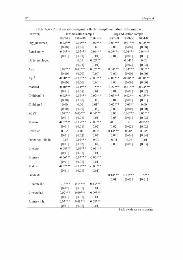
4.4.3 Self-employment

As explained above, self-employed women have been excluded from the unit level

analysis because their earnings are not available and one cannot reliably estimate expected

market earnings for this group.30 In order to check whether this has a big impact on the

probit results, the participation model is re-estimated without the predicted wage (instead,

age and age squared are included directly in the participation model). This model is then

estimated separately for each year and education group, both with and without the self-

employed in the sample. While we cannot conclude anything regarding the own wage

30 In the preceding estimations, self-employed earnings are imputed for other household members in order to calculate unearned income. As mentioned in section 4.4.1, the resulting measure of unearned income gives the same results compared to excluding any households with self-employed members from the sample. However, this is not deemed sufficient indication that one can use the same imputation for women’s own wage: self-employment earnings are only a part of unearned income while they would constitute the entire own wage of self-employed women, which is thus much more sensitive to the imputation method.

Chapter 4

80

effect on participation in self-employment, the main results do not depend on the exclusion

of self-employed women.

The results excluding the own wage effect, but still restricting the sample to exclude

self-employed women (not shown), indicate that own education picks up the own wage

effect for the highly educated: it has a higher marginal effect, which declines over time

from 0.18 to 0.16. Age has a positive effect, somewhat higher for the highly educated, and

age squared has a negative effect. Estimates of the other marginal effects hardly differ.

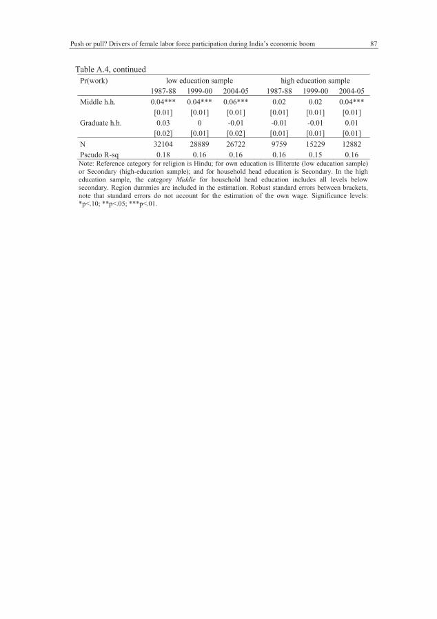
Next, adding the self-employed to the sample, there are changes in some of the marginal

effects (see Appendix Table A.4 for the estimates). First, the negative effect of marriage is

stronger in each year and in both samples. Second, the negative effect of household head

education becomes stronger in the low-education sample. If household head education is

taken as a proxy for status, this result is a bit surprising. Since women’s self-employment,

often taking place within the household, is less subject to social stigma, one would expect

that including self-employment would reduce the negative effect of head’s education.

However, we see that the effect gets stronger, so it might be more related to household

wealth and the necessity of women’s work in the poorest households.

Finally, the marginal effect of the regular-earnings share of unearned income declines

and even becomes negative in the low-education sample: the probability of paid

employment increases with the regular employment of household members, but the

probability of self-employment apparently does not. It is therefore likely that regular

employees in the household indeed have a network effect or familiarity effect enhancing

only the paid employment, but not self-employment, of women.

An important note here is that the determinants of self-employment may be different

from those of paid employment, because self-employed women typically contribute to a

family business and thus often carry out their ‘market work’ inside the household.

Restrictions due to social stigma and the double burden of household work and market

work are therefore rather different between paid employment and self-employment.

Besides our inability to estimate an own-wage effect on participation in self-employment,

therefore, a more general caveat of the present chapter is the fact that the basic labor

supply model may not give us much insight into women’s participation in self-

employment. In urban India, however, the majority of working women has paid

employment, so our analysis should present a good picture of the drivers of female labor

force participation in urban India.


81

4.5 Summary and conclusions

While India’s economy has grown at increasingly faster rates over the past decades, the

female labor force participation rate has increased only since the start of the 21st century,

when at all levels of education the share of women in the labor force increased. This

chapter examines trends and drivers of female labor force participation in urban India

between 1987 and 2004, paying special attention to differences between lowly and highly

educated women.

Changes in the structure of employment and real earnings in urban India suggest that

increased participation of women with less than secondary schooling was driven more by

necessity rather than improved opportunities. After 1999, the share of poorly educated

women working as domestic servant and in agriculture and manufacturing self-

employment increased, the latter concentrated in the garments industry. Domestic servants

and home workers in the garments industry have been characterized by their invisibility,

vulnerability, and meager and highly volatile earnings (NCEUS, 2007; Singh and Sapra,

2007). Coinciding with substantial growth in these types of employment, workers with less

than secondary education, both male and female, experienced a decline in their real

earnings.

For the poorly educated urban population, therefore, the labor market trends are in line

with the view of Standing (1999), who argues that female labor force participation is

driven by the erosion of men’s position in the labor market, rather than improvements in

women’s opportunities: workers face more insecurity as economies liberalize and become

more globally integrated. Our unit level analysis in section 4.4 shows that participation of

women with less than secondary education is not affected by their own earnings potential,

but predominantly driven by economic push factors and social status of the household (in

line with Kingdon and Unni, 2001; Sudarshan and Bhattacharya, 2009).

The picture for highly educated women looks different. Real earnings of men and

women with graduate level education did still rise after 1999, though at a slower rate than

before. Among highly educated women, self-employment in manufacturing and services

became more important, but regular employment in services increased as well. These

women, or at least some of them, appear to have access to more attractive jobs in terms of

visibility, security, and earnings. Given India’s structure of growth, which is in large part

driven by skill-intensive services, this should hardly be surprising. The unit level

estimation results indeed show that highly educated women, as opposed to the poorly

educated, are drawn into the labor force by higher wages. Their own education, moreover,

Chapter 4

82

has a positive effect on participation, while household head’s education has no effect. The

effect of unearned income is similar as for the poorly educated, so overall the highly

educated women behave more in line with the standard models of labor supply.

To conclude, our analysis indicates that the impressive economic performance of the

Indian economy is, if anything, only creating attractive labor market opportunities for

highly educated women. The urban labor market for poorly educated women (and men)

does not seem to be improving at all, and there is no evidence that increased participation

among them is a positive reflection of India’s fast economic growth. It always remains

debatable whether increased participation in low-paying and informal jobs should be seen

as improvements compared to non-participation. For whatever reason women decide to

work, it does allow them to contribute to household income. One could surely also argue

that home workers in the garments industry, for example, contribute to India’s economic

success. As Bhalotra and Umaña-Aponte (2010) argue, however, distress-driven

participation in a highly flexible labor market is unlikely to contribute to women’s

empowerment. Since for Indian women with little education, push factors and household

social status are major determinants of participation, while own earnings potential plays no

role, their participation can hardly be considered a sign of emancipation.


83

Appendix

Table A.1 - Urban females (age 20-59) by employment status and industry

Below secondary education 1987-88 1993-94 1999-00 2004-05Agriculture Self-employed 870 (2.5) 876 (2.2) 744 (1.7) 1,265 (2.5) Regular 35 (0.1) 37 (0.1) 56 (0.1) 73 (0.1) Casual 861 (2.5) 1,173 (2.9) 1,124 (2.6) 1,080 (2.1)Manufacturing Self-employed 1,024 (3.0) 1,137 (2.9) 1,383 (3.1) 2,004 (4.0) Regular 362 (1.1) 312 (0.8) 517 (1.2) 641 (1.3) Casual 508 (1.5) 570 (1.4) 316 (0.7) 430 (0.9)Other industry Self-employed 12 (0.0) 16 (0.0) 11 (0.0) 11 (0.0) Regular 58 (0.2) 58 (0.1) 51 (0.1) 48 (0.1) Casual 393 (1.2) 567 (1.4) 683 (1.6 757 (1.5)Services Self-employed 1,046 (3.1) 1,388 (3.5) 1,802 (4.1) 1,896 (3.8) Regular 1,054 (3.1) 1,274 (3.2) 1,432 (3.3) 2,450 (4.9) Casual 431 (1.3) 617 (1.5) 760 (1.7) 620 (1.2)Workforce 6,654(19.4) 8,023(20.1) 8,879(20.2) 11,273(22.4)Unemployed 285 (0.8) 207 (0.5) 158 (0.4) 362 (0.7)Other 27,364(79.8) 31,612(79.4) 34,926(79.4) 38,672(76.9)Total 34,304(100) 39,838(100) 43,965(100) 50,308(100) Secondary education or higher 1987-88 1993-94 1999-00 2004-05Agriculture Self-employed 25 (0.3) 32 (0.2) 21 (0.1) 78 (0.3) Regular 2 (0.0) 1 (0.0) 3 (0.0) 5 (0.0) Casual 5 (0.0) 14 (0.1) 12 (0.1) 12 (0.0)Manufacturing Self-employed 98 (1.0) 111 (0.7) 168 (0.7) 437 (1.5) Regular 138 (1.4) 203 (1.3) 263 (1.1) 410 (1.4) Casual 4 (0.0) 22 (0.1) 27 (0.1) 29 (0.1)Other industry Self-employed 5 (0.1) 6 (0.0) 9 (0.0) 14 (0.0) Regular 29 (0.3) 41 (0.3) 35 (0.1) 74 (0.2) Casual 6 (0.1) 5 (0.0) 12 (0.1) 3 (0.0)Services Self-employed 154 (1.5) 363 (2.3) 609 (2.6) 971 (3.3) Regular 1,654(16.5) 2,361(14.8) 3,008(12.9) 3,952(13.3) Casual 9 (0.1) 13 (0.1) 36 (0.2) 24 (0.1)Workforce 2,130(21.3) 3,173(19.9) 4,201(18.0) 6,009(20.2)Unemployed 498 (5.0) 769 (4.8) 754 (3.2) 1,364 (4.6)Other 7,392(73.8) 11,984(75.2) 18,381(78.8) 22,349(75.2)Total 10,020 (100) 15,928 (100) 23,335 (100) 29,724 (100)

Note: Numbers are in thousands, the percentage of total is given in parentheses. Agriculture includes forestry and fishing. Other industry includes mining, construction, and utilities. Self-employment includes own account workers, home workers, employers, and unpaid family workers. Regular employees receive salary or wages on a regular basis. Casual workers receive a wage according to the terms of the daily or periodic work contract. “Other” includes all non-labor force and a small number of women who work but do not report their industry. Source: NSS Employment and Unemployment Survey, population totals from Sundaram (2007).

Chapter 4

84

Table A.2 - Wage equation, estimation results Below secondary education Secondary or higher education

ln w 1987-88 1999-00 2004-05 1987-88 1999-00 2004-05

Age 0.03** 0.03* 0.03** 0.12*** 0.11*** 0.09*** [0.01] [0.01] [0.01] [0.01] [0.01] [0.02] Age sq. 0.00 0.00 -0.00* -0.00*** -0.00*** -0.00** [0.00] [0.00] [0.00] [0.00] [0.00] [0.00] Illiterate Ref. Ref. Ref. Literate 0.12* 0.17*** 0.15*** [0.05] [0.05] [0.04] Primary 0.15** 0.13** 0.13*** [0.05] [0.05] [0.04] Middle 0.53*** 0.26*** 0.25*** [0.06] [0.05] [0.04] Secondary Ref. Ref. Ref. Graduate 0.52*** 0.50*** 0.60*** [0.04] [0.04] [0.05] Constant 2.81*** 3.34*** 3.28*** 2.50*** 2.60*** 2.66*** [0.21] [0.22] [0.18] [0.24] [0.27] [0.27] Lambda 0.22*** 0.21*** 0.14*** 0.16*** 0.16*** 0.21*** [0.04] [0.04] [0.03] [0.04] [0.05] [0.05] N 2264 2182 2623 1755 2125 1891

Note: Dependent variable is log real weekly earnings. Lambda is the sample selection bias correction term (see Heckman, 1979). Standard errors are in brackets, significance levels: *p<.10; **p<.05; ***p<.01

Table A.3 - Wage model selection equation, estimation results

Below secondary education Secondary or higher education

Pr(employee) 1987-88 1999-00 2004-05 1987-88 1999-00 2004-05

Age 0.09*** 0.11*** 0.10*** 0.20*** 0.14*** 0.13***

[0.01] [0.01] [0.01] [0.02] [0.01] [0.01]

Age sq. -0.00*** -0.00*** -0.00*** -0.00*** -0.00*** -0.00***

[0.00] [0.00] [0.00] [0.00] [0.00] [0.00]

Illiterate

Literate -0.20*** -0.24*** -0.20***

[0.04] [0.04] [0.04]

Primary -0.39*** -0.40*** -0.36***

[0.04] [0.04] [0.04]

Middle -0.41*** -0.48*** -0.48***

[0.05] [0.04] [0.04]

Secondary Ref. Ref. Ref.

Graduate 0.72*** 0.78*** 0.74***

[0.04] [0.03] [0.03] Table continues on next page


85

Table A.3, continued

Below secondary education Secondary or higher education

Pr(employee) 1987-88 1999-00 2004-05 1987-88 1999-00 2004-05

ln(y_unearned) -0.17*** -0.12*** -0.16*** -0.13*** -0.08*** -0.13***

[0.01] [0.01] [0.01] [0.02] [0.01] [0.01]

Regshare_y 0.16*** 0.05 0.10*** 0.55*** 0.50*** 0.51***

[0.03] [0.03] [0.03] [0.04] [0.03] [0.04]

Illiterate h.h. 0.80*** 0.82*** 0.70***

[0.05] [0.05] [0.05]

Literate h.h. 0.53*** 0.55*** 0.45***

[0.05] [0.05] [0.05]

Primary h.h. 0.42*** 0.49*** 0.45***

[0.05] [0.05] [0.05]

Middle h.h. 0.30*** 0.28*** 0.35*** -0.03 0.09* 0.09*

[0.06] [0.05] [0.05] [0.05] [0.04] [0.04]

Secondary h.h.

Graduate h.h. 0.45*** 0.28*** 0.14 -0.08 -0.04 0.06

[0.07] [0.08] [0.08] [0.04] [0.03] [0.04]

Married -0.53*** -0.59*** -0.66*** -0.98*** -0.92*** -1.04***

[0.04] [0.04] [0.04] [0.05] [0.05] [0.05]

Children0-4 -0.11*** -0.18*** -0.17*** -0.09*** -0.10*** -0.20***

[0.02] [0.02] [0.02] [0.03] [0.02] [0.03]

Children 5-14 -0.04*** -0.04*** 0.00 -0.09*** -0.07*** -0.03

[0.01] [0.01] [0.01] [0.02] [0.02] [0.02]

SCST 0.44*** 0.39*** 0.31*** 0.24** 0.32*** 0.25***

[0.03] [0.03] [0.03] [0.08] [0.05] [0.05]

Muslim -0.36*** -0.62*** -0.60*** -0.14 0.05 -0.15*

[0.04] [0.04] [0.04] [0.08] [0.06] [0.06]

Christian 0.34*** 0.17* -0.04 0.54*** 0.39*** 0.35***

[0.07] [0.08] [0.08] [0.08] [0.06] [0.07]

Other non-Hindu -0.05 -0.40*** -0.13 -0.18* -0.08 -0.06

[0.08] [0.09] [0.08] [0.07] [0.06] [0.07]

constant -2.49*** -2.53*** -1.91*** -3.66*** -3.33*** -2.44***

[0.19] [0.20] [0.19] [0.27] [0.24] [0.25]

N 29618 26429 24067 9515 14695 12119 Note: Table shows estimated probit coefficients, with robust standard errors in brackets. Region dummies are included in the estimation, but not reported. Significance levels: *p<.10; **p<.05; ***p<.01

Chapter 4

86

Table A.4 - Probit average marginal effects, sample including self-employed Pr(work) low education sample high education sample 1987-88 1999-00 2004-05 1987-88 1999-00 2004-05

ln(y_unearned) -0.02*** -0.02*** -0.02*** -0.03*** -0.01*** -0.02*** [0.00] [0.00] [0.00] [0.00] [0.00] [0.00] Regshare_y -0.04*** -0.07*** -0.06*** 0.09*** 0.06*** 0.04*** [0.01] [0.01] [0.01] [0.01] [0.01] [0.01] Underemployed 0.01 0.02*** 0.04** 0.02 [0.01] [0.01] [0.02] [0.02] Age 0.02*** 0.02*** 0.02*** 0.04*** 0.03*** 0.03*** [0.00] [0.00] [0.00] [0.00] [0.00] [0.00] Age2 -0.00*** -0.00*** -0.00*** -0.00*** -0.00*** -0.00*** [0.00] [0.00] [0.00] [0.00] [0.00] [0.00] Married -0.10*** -0.11*** -0.15*** -0.22*** -0.21*** -0.24*** [0.01] [0.01] [0.01] [0.01] [0.01] [0.02] Children0-4 -0.02*** -0.02*** -0.02*** -0.03*** -0.02*** -0.05*** [0.00] [0.00] [0.00] [0.01] [0.01] [0.01] Children 5-14 0.00 0.00 0.01* -0.02*** -0.01** 0.00 [0.00] [0.00] [0.00] [0.00] [0.00] [0.00] SCST 0.07*** 0.05*** 0.04*** 0.05 0.06*** 0.06*** [0.01] [0.01] [0.01] [0.03] [0.01] [0.02] Muslim -0.07*** -0.09*** -0.09*** -0.01 0 -0.05** [0.01] [0.01] [0.02] [0.02] [0.02] [0.02] Christian 0.03* -0.01 -0.02 0.14*** 0.08* 0.08* [0.01] [0.02] [0.02] [0.04] [0.04] [0.04] Other non-Hindu -0.02 -0.07*** -0.03 -0.04 -0.02 -0.01 [0.01] [0.02] [0.02] [0.03] [0.02] [0.03] Literate -0.04*** -0.04*** -0.05*** [0.01] [0.01] [0.01] Primary -0.06*** -0.07*** -0.06*** [0.01] [0.01] [0.01] Middle -0.07*** -0.08*** -0.08*** [0.01] [0.01] [0.01] Graduate 0.18*** 0.17*** 0.15*** [0.01] [0.01] [0.01] Illiterate h.h. 0.16*** 0.14*** 0.13*** [0.02] [0.01] [0.01] Literate h.h. 0.09*** 0.09*** 0.09*** [0.01] [0.01] [0.01] Primary h.h. 0.07*** 0.08*** 0.08*** [0.01] [0.01] [0.01]

Table continues on next page


87

Table A.4, continued Pr(work) low education sample high education sample 1987-88 1999-00 2004-05 1987-88 1999-00 2004-05

Middle h.h. 0.04*** 0.04*** 0.06*** 0.02 0.02 0.04*** [0.01] [0.01] [0.01] [0.01] [0.01] [0.01] Graduate h.h. 0.03 0 -0.01 -0.01 -0.01 0.01 [0.02] [0.01] [0.02] [0.01] [0.01] [0.01]

N 32104 28889 26722 9759 15229 12882 Pseudo R-sq 0.18 0.16 0.16 0.16 0.15 0.16 Note: Reference category for religion is Hindu; for own education is Illiterate (low education sample) or Secondary (high-education sample); and for household head education is Secondary. In the high education sample, the category Middle for household head education includes all levels below secondary. Region dummies are included in the estimation. Robust standard errors between brackets, note that standard errors do not account for the estimation of the own wage. Significance levels: *p<.10; **p<.05; ***p<.01.

Documents

University of Groningen Essays on socio-economic