Embed Size (px)
Citation preview
University of Groningen
Non-relativistic supergravity in three space-time dimensionsZojer, Thomas
IMPORTANT NOTE: You are advised to consult the publisher's version (publisher's PDF) if you wish to cite fromit. Please check the document version below.
Document VersionPublisher's PDF, also known as Version of record
Publication date:2016
Link to publication in University of Groningen/UMCG research database
Citation for published version (APA):Zojer, T. (2016). Non-relativistic supergravity in three space-time dimensions. University of Groningen.
CopyrightOther than for strictly personal use, it is not permitted to download or to forward/distribute the text or part of it without the consent of theauthor(s) and/or copyright holder(s), unless the work is under an open content license (like Creative Commons).
The publication may also be distributed here under the terms of Article 25fa of the Dutch Copyright Act, indicated by the “Taverne” license.More information can be found on the University of Groningen website: https://www.rug.nl/library/open-access/self-archiving-pure/taverne-amendment.
Take-down policyIf you believe that this document breaches copyright please contact us providing details, and we will remove access to the work immediatelyand investigate your claim.
Downloaded from the University of Groningen/UMCG research database (Pure): http://www.rug.nl/research/portal. For technical reasons thenumber of authors shown on this cover page is limited to 10 maximum.
Download date: 02-02-2022

Non-relativistic supergravityin three space–time dimensions
Proefschrift
ter verkrijging van de graad van doctor aan deRijksuniversiteit Groningen
op gezag van derector magnificus prof. dr. E. Sterken
en volgens besluit van het College voor Promoties.
De openbare verdediging zal plaatsvinden op
maandag 4 januari om 11.00 uur
door
Thomas Zojer
geboren op 7 augustus 1987te Wenen, Oostenrijk
PromotorProf. dr. E. A. Bergshoeff
BeoordelingscommissieProf. dr. N. ObersProf. dr. S. VandorenProf. dr. D. Roest
ISBN 978-90-367-8487-0 (printed)ISBN 978-90-367-8486-3 (digital)
Contents
1 Introduction 51.1 Newton–Cartan (like) structures in physics . . . . . . . 71.2 Non-relativistic (super)symmetry . . . . . . . . . . . . 81.3 Outline of the thesis . . . . . . . . . . . . . . . . . . . . 11
2 Background material 152.1 Conventions . . . . . . . . . . . . . . . . . . . . . . . . 162.2 Gauge symmetries . . . . . . . . . . . . . . . . . . . . . 172.3 Symmetry algebras . . . . . . . . . . . . . . . . . . . . 202.4 Gauging the Poincare algebra . . . . . . . . . . . . . . 212.5 Non-relativistic gravity . . . . . . . . . . . . . . . . . . 252.6 Spinors . . . . . . . . . . . . . . . . . . . . . . . . . . . 312.7 Global supersymmetry . . . . . . . . . . . . . . . . . . 342.8 Local supersymmetry: supergravity . . . . . . . . . . . 36
3 A non-relativistic limiting procedure 413.1 The general procedure . . . . . . . . . . . . . . . . . . 423.2 Newton–Cartan gravity . . . . . . . . . . . . . . . . . . 453.3 Non-relativistic N = 1 supergravity . . . . . . . . . . 513.4 On-shell Newton–Cartan supergravity . . . . . . . . . 543.5 3D non-relativistic off-shell supergravity . . . . . . . . 593.6 The point-particle limit . . . . . . . . . . . . . . . . . . 643.7 Conclusion . . . . . . . . . . . . . . . . . . . . . . . . . 68
4 Newton–Hooke supergravity 714.1 The Newton–Hooke superalgebra . . . . . . . . . . . . 734.2 Gauging the Newton–Hooke superalgebra . . . . . . . 764.3 Galilean Newton–Hooke supergravity . . . . . . . . . 814.4 Connection to the non-relativistic limit . . . . . . . . . 874.5 Summary . . . . . . . . . . . . . . . . . . . . . . . . . . 90
5 Schrodinger supergravity 915.1 A Schrodinger superalgebra . . . . . . . . . . . . . . . 935.2 Gauging . . . . . . . . . . . . . . . . . . . . . . . . . . . 945.3 Concluding remarks . . . . . . . . . . . . . . . . . . . . 103
6 Schrodinger tensor calculus 1056.1 Matter couplings . . . . . . . . . . . . . . . . . . . . . . 1076.2 Newton–Cartan supergravity with torsion . . . . . . . 1146.3 Truncation to zero torsion . . . . . . . . . . . . . . . . . 1216.4 A brief summary . . . . . . . . . . . . . . . . . . . . . . 124
7 Conclusion 1257.1 Summary of the thesis . . . . . . . . . . . . . . . . . . . 1267.2 Outlook . . . . . . . . . . . . . . . . . . . . . . . . . . . 129
List of publications 133
References 135
Samenvatting 145
Acknowledgements 153

1Introduction
This chapter shall serve as a motivation for the analysis performed in this thesis.We aim to motivate the problem, put it into context and briefly describe it withas little technical detail as possible.
6 Introduction
Gravitation is the only unquestionably ubiquitous, fundamental force in Nature.It is so common to us that we can hardly envision a world without it. Obviously,it was also the first one subject to investigation by physicists. Newton and Ke-pler were the first to successfully describe the motion of particles and planets thatundergo gravitational interactions. Nowadays though, we believe that Newton’stheory is but an effective description of another more fundamental theory, the the-ory of general relativity that was formally described first by Einstein exactly onehundred years ago, see e.g. [1].
Einstein’s theory rests only on a few pillars, statements that give restrictions,certain laws that the theory should obey. Notably, one of them is that the the-ory must be independent of the coordinate system that is used to describe it. Incontemporary (theoretical, but not exclusively) physics this is an obvious thingto do, i.e. one requires invariance of the theory and its predictions under generalcoordinate transformations. In hindsight though, we might wonder why no oneaddressed this question for the Newtonian theory. Even before the discovery ofgeneral relativity, the concept of diffeomorphism invariance could have been ad-dressed for any theory that has so far only been formulated in such a way that it isinvariant under Galilean coordinate transformations.
At the time, this might have been sufficient. Physical models were mostly con-sidered in so-called free-falling, or inertial, frames. These are coordinate frameswhere an observer is not subject to any gravitational force. Different non-relativ-istic inertial frames are then related by Galilean coordinate transformations. (Inthe relativistic context these would be the Lorentz transformations.) Galilean trans-formations relate two different coordinate systems via constant rotations, boostsand shifts. In contrast, arbitrary general coordinate transformations are not sub-ject to any limitation, such as constancy of the symmetry parameters. As men-tioned before, in the context of non-relativistic theories, one oftentimes considersonly Galilean transformations. However, in principle there should exist a descrip-tion of any non-relativistic theory, and thus of Newtonian gravity, that is invariantunder arbitrary transformations of the coordinates.
So, what is the coordinate independent description of Newtonian gravity? Onlya few years after Einstein’s discovery of general relativity this question was even-tually answered. It was discovered by the French mathematician Cartan and thetheory now goes by the name Newton–Cartan gravity [2, 3]. It is this coordinateindependent description of Newtonian gravity that we are most concerned with inthis thesis. Note that, while the Newton–Cartan theory obeys one of the statementsthat Einstein’s theory is based on, it does differ from general relativity in anothercrucial aspect. Namely, in the Newton–Cartan theory there exists no maximal ve-locity. We come back to this issue in chapter 3 when we investigate how Einstein’stheory gets deformed when we let its limiting speed, the speed of light, go to in-finity. As we shall see this provides one way to derive the Newton–Cartan theoryfrom general relativity.
1.1 NEWTON–CARTAN (LIKE) STRUCTURES IN PHYSICS 7
1.1 Newton–Cartan (like) structures in physicsMost of the recent interest in describing theories that are invariant under non-relativistic general coordinate transformations has been stirred by developments incondensed matter theories, see e.g. [4–7] for some earlier works. This engenderedmore systematic studies recently, especially on how to couple non-relativistic fieldtheories to Newton–Cartan backgrounds [8–17] (see also [18–24]). It has been notedthat besides the “usual” fields, the time-like and spatial vielbein, one needs an addi-tional vector field to consistently couple non-relativistic field theories to arbitrarycurved backgrounds, see in particular [8–11] and [16]. These references togetherwith [25–29] also point towards another important aspect of the background geom-etry: that one should not restrict the torsion of the non-relativistic gravity theory.
The necessity to add an extra vector gauge-field to the Newton–Cartan fieldswas also realized by Son [30]. The use of Newton–Cartan structures is obligatoryin his effective action for the quantum Hall effect [8, 30–33]. This model naturallyincludes a so-called Wen–Zee term [34], which describes the coupling between theextra gauge-field and the curvature, thus encoding the Hall viscosity and givingrise to more universal features of the quantum Hall effect than only the quantizedHall conductivity. Through a similar coupling with a U(1) gauge-field and a Wen–Zee term, one obtains an effective action for chiral superfluids as well [35, 36]. Itwas realized in [36] that Newton–Cartan structures offer a particularly neat wayto write the action in a covariant form, and hence offer a convenient framework tocalculate e.g. the energy current of the superfluid. Newton–Cartan structures arealso essential in describing Newtonian fluids [37, 38]. In particular, those modelswere used to describe the effects of superfluidity in Neutron stars [38–40]. A studyof non-relativistic fluids, or “Galilean fluids”, i.e. hydrodynamics on Galilean back-grounds features in [41, 42]. Indeed, the applications of Newton–Cartan structuresin describing effective actions for phenomena in condensed matter physics seem sovast that this short introduction can hardly do justice to all works in this fields.
Some works on condensed matter theory are motivated by the emergence ofnew “holographic” techniques in condensed matter physics, see [43–46]. Thesetechniques lend their roots to the holographic principle [47, 48], which is a con-jectured correspondence of gravitational theories in anti-de Sitter space-times andconformal field theories, the so-called AdS/CFT correspondence. Some simple, yetinsightful, manifestations of this duality were found in three-dimensional space-times, see e.g. [49–51], building on the seminal work of Brown and Henneaux [52],which is indeed one of the precursors for this duality. While, as we mentioned be-fore, such techniques are already being applied, much still needs to be investigatedwhen it comes to test the generality of this correspondence. The work on find-ing non-relativistic realizations of this duality is one effort in this direction. Moreconcretely, let us draw the attention to the recent works [15,25–27] where Newton–Cartan structures play a very prominent role.
Newton–Cartan like structures, in fact dual structures that are more related toultra-relativistic physics than non-relativistic physics, also feature in warped con-

8 Introduction
formal field theories [53, 54]. They are also conjectured to play a role in the ten-sionless limit of string theory [55, 56]. The tensionless limit amounts to taking anultra-relativistic limit [55, 57], that leads to “Carrollian” physics and space-times,which are in many ways dual to Newton–Cartan structures, see e.g. [54, 55, 57–61].Other, in fact opposite, non-relativistic limits of string theory have also been con-sidered. Non-relativistic string theory [62, 63] was studied as a possible solublesector within string or M-theory [64–70]. These works are also important for theapplications of the holographic principle in the context of condensed matter theorywhich we mentioned before.
A more systematic approach towards non-relativistic (and ultra-relativistic) ge-ometry was taken in [71, 72], where Newton–Cartan structures are discussed witha particular emphasis on the metric structures.
In this thesis we will be mostly interested in supersymmetric extensions ofNewton–Cartan structures. While we will discuss (non-relativistic) supersymme-try more at a later stage, let us give some motivations for our general interest inthem here. For example, one of the papers on the quantum Hall effect does infact make use a (non-relativistic) supersymmetric model [73]. Further motivations,and indeed one of the main motivations for this thesis in general, is related to thevery successful application of localization techniques in the relativistic context, seee.g. [74, 75]. The applications of localization techniques have proved useful to ob-tain exact results for relativistic supersymmetric field theories. Perhaps we can ex-pect similarly successful results in the non-relativistic case too. The method relieson the coupling of non-relativistic field theories to arbitrary supersymmetric back-grounds. To do so, one needs of course non-relativistic supergravity theories toprovide such backgrounds. However, the construction that we have in mind [76],makes use of so-called off-shell formulations of supergravity, a feature that the onlyknown theory of non-relativistic supergravity so far, see [77], does not possess.Suitable extensions of Newton–Cartan supergravity would be necessary to checkwhether those techniques can be extended to non-relativistic theories.
We discussed the main motivations for our interest in non-relativistic physicsand that Newton–Cartan structures provide a convenient way of denoting the non-relativistic gravity background. Moreover, we gave one particular motivation toconsider supersymmetric theories. Let us now return to the point where we started:symmetries.
1.2 Non-relativistic (super)symmetryRequiring a theory, Newtonian gravity in this case, to be invariant under general co-ordinate transformations, means that it should be invariant under a special kind ofsymmetry transformation. Symmetries play a major role in contemporary theoret-ical physics. They impose strong restrictions on a theory, for example they restrictthe kind of interaction terms that one can write down. This is of vital importance asparticular symmetries of a given theory can often be found in experiments and thus

1.2 NON-RELATIVISTIC (SUPER)SYMMETRY 9
the underlying “fundamental” theory can be much better described. All (quantum)theories that are used to describe the standard model of particle physics are gauge-theories, i.e. they are by construction invariant under a certain symmetry. The sym-metry groups are U(1) for electrodynamics, SU(2) for the weak interactions andSU(3) for the strong interactions. In a way, general relativity can be understoodas a gauge-theory too. It is the gauge-theory of diffeomorphisms. As we will seelater, this feature, the gauge-theory aspect of general relativity, is of particular im-portance to us.
In view of such vast applications, an interesting question is what is the mostgeneral symmetry (group) that we can allow? This has been extensively studiedand one of the most celebrated theorems by Coleman and Mandula [78] statesthat a physical theory can at most be invariant under the conformal group. Allother symmetries must be “internal” ones, i.e. physical observables must alwaysbe scalar representations of those symmetries. This theorem holds but for one ex-ception: it does not account for fermionic symmetries. As was later shown by Haag,Lopuszanski and Sohnius [79] the addition of supersymmetry, or superconformalsymmetries to be precise, really exhausts all possibilities. This, in a way, funda-mental nature of supersymmetry serves as one more motivation for us to considersupersymmetric theories and to study supersymmetric Newton–Cartan structuresin this thesis.
We must now put our focus more towards non-relativistic symmetries. To un-derstand how a theory can be invariant under non-relativistic diffeomorphisms onemust of course know what non-relativistic diffeomorphisms are. Interestingly, thisis part of current research too. One approach consists of mimicking some ideas thatcan be applied to general relativity as well. General relativity can be seen as gauge-theory of the Poincare algebra and hence one could try to derive a non-relativisticversion thereof by gauging instead a non-relativistic symmetry algebra. This ap-proach was pursued in [77, 80]. In particular, in [77] it was shown how the gauge-theory of the Bargmann algebra can be reduced to Newtonian gravity by gauge-fixing. The Newton–Cartan theory was thus linked to Newtonian gravity and itwas shown explicitly that the difference between those theories is precisely due tothe amount of symmetry that we allow. We will apply similar ideas, i.e. gaugingtechniques, to derive some of the new (supergravity) theories that we put forwardin this thesis.
Let us pause for a moment to fix nomenclature and to quickly define the dif-ferent theories of non-relativistic gravity. Newton–Cartan gravity is invariant un-der general coordinate transformations, while in Newtonian gravity we allow onlyfor Galilei transformations with constant symmetry parameters. There is one in-between step that we shall also consider in this thesis. We can allow for arbi-trary time-dependent spatial translations, keeping all other symmetry parametersconstant. These symmetries are sometimes referred to as “acceleration-extended”Galilean symmetries, or Milne symmetries [4]. The theory is then called Galileangravity.
What kind of non-relativistic symmetries will we be interested in? We already
10 Introduction
mentioned Galilean symmetries and also the Bargmann algebra. Just like in the rel-ativistic case, we can extend those with yet more symmetry generators. In the rela-tivistic case this leads to conformal symmetry. In the non-relativistic case however,we have the choice between two different “conformal” extensions of the Galileialgebra. The Galilean conformal algebra [46, 81] is the non-relativistic analog ofthe conformal algebra. Another possibility is the Schrodinger algebra [82, 83]. Wewill choose to work with the latter one because it is the only possible extension ofthe Bargmann algebra.1 This in particular implies that we can allow for non-zeromass.2 Indeed, the additional symmetry of the Bargmann algebra (w.r.t. the Galileialgebra) is often interpreted as being related to the conservation of mass (and beingnon-relativistic this implies conservation of particle number).
The Schrodinger algebra comprises symmetry generators which give rise to thesymmetries of the Schrodinger equation (hence the name). The rigid Schrodingertransformations also leave invariant the simple action of the non-relativistic point-particle:
S =m2
∫dt xi xi .
More extensions of this formula will also follow in this thesis.So, in the spirit of Coleman–Mandula we add “conformal” extensions. But in
this thesis in particular, we will also be interested in another extension of non-relati-vistic symmetries, namely the addition of supersymmetry.
Above we gave some “physical” reasons to study Newton–Cartan theories andalso for studying supersymmetry in that context. Another motivation comes fromthe analysis of [78, 79] in the relativistic context. In the relativistic case, supersym-metry or superconformal symmetries are the most general symmetries that we canallow for a theory. In the non-relativistic case, there are no arguments similar tothose of [78, 79], but it is still interesting to see if we are even able to find non-relativistic theories that are supersymmetric.
Non-relativistic supersymmetry algebras are not per se difficult to construct andsome simple field theories that realize those symmetries have also been found, seee.g. [84–94]. However, the first local realization of non-relativistic supersymmetrydates back only to the year 2013 [77]. There are no (known) obstacles that wouldprevent anyone from finding such theories in principle. However, it turns out thatthis is not an easy task and one faces quite some difficulties. This leads us to firstconsent ourselves with constructing examples in a simpler setting. Such simplicitycan result for example from considering theories in lower dimensions. Therefore,the non-relativistic supergravity theories that we will construct in this thesis, all ofwhich are generalizations of [77], are theories in three space-time dimensions. We
1 We will discuss the reasons for our particular interest in the Bargmann algebra instead of the Galileialgebra at a later stage, as they are mostly technical in nature.
2 In the relativistic case, conformal symmetry is too strong to allow for massive representations.Therefore, since our “conformal” Schrodinger symmetry does allow m 6= 0, we will reserve the name(non-relativistic) conformal symmetry for the Galilean conformal ones.
1.3 OUTLINE OF THE THESIS 11
hope that a more thorough understanding of the mechanics of three-dimensionalcase will provide useful insight for the construction of four-dimensional theories.
1.3 Outline of the thesisSo, this thesis deals with non-relativistic supergravity theories in three space-timedimensions. We motivated our interest in such theories, which stems from effectivemodels in condensed matter theory to possible applications of localization tech-niques. The fact that we work in three dimensions is due to a more straightforwardmotto of ours: simplicity first. In the following we will work out many examplesof non-relativistic supergravity theories and shall compare our findings with therelativistic case.
At first we must address the question of how we are going to construct those su-pergravities. Throughout this work we will use two different techniques. The firstone lends its roots to relativistic supergravity and the fact that it can be obtainedby gauging the Poincare superalgebra [95]. The application of similar techniqueswill allow us to obtain non-relativistic supergravities by gauging non-relativisticsuperalgebras instead. This approach will feature in chapters 4 and 5. The othermethod to derive non-relativistic supergravities is a non-relativistic limiting proce-dure that we develop in chapter 3. This method is also used in chapter 6 to derivenon-relativistic matter multiplets.
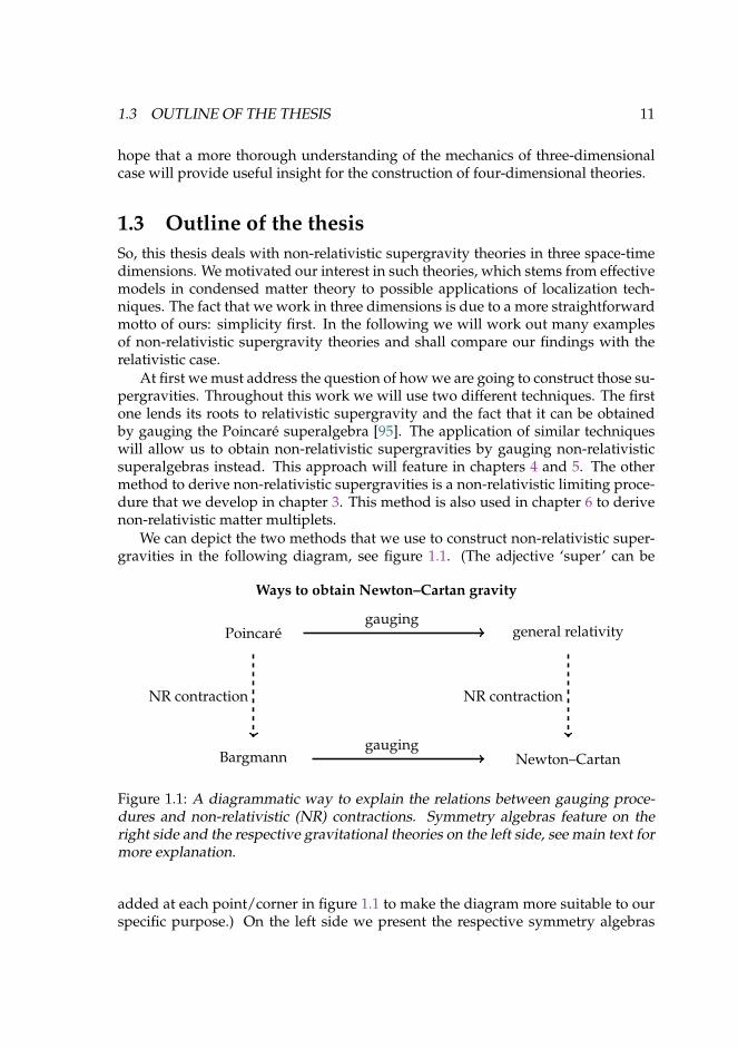
We can depict the two methods that we use to construct non-relativistic super-gravities in the following diagram, see figure 1.1. (The adjective ‘super’ can be
Ways to obtain Newton–Cartan gravity
Poincare
Bargmann
general relativity
Newton–Cartan
NR contraction NR contraction
gauging
gauging
Figure 1.1: A diagrammatic way to explain the relations between gauging proce-dures and non-relativistic (NR) contractions. Symmetry algebras feature on theright side and the respective gravitational theories on the left side, see main text formore explanation.
added at each point/corner in figure 1.1 to make the diagram more suitable to ourspecific purpose.) On the left side we present the respective symmetry algebras
12 Introduction
that are gauged. The horizontal arrows stand for the gauging procedures, e.g. theupper line translates to “general relativity can be obtained by gauging the Poincarealgebra”. The dashed, vertical arrow on the left corresponds to the Inonu–Wignercontraction [96], which is a way to obtain the Bargmann (super)algebra from thePoincare (super)algebra. The dashed arrow on the right stands for the limiting pro-cedure that we adopt in chapter 3. It is no coincidence that this graph seems tosuggest the limiting procedure is motivated by the Inonu–Wigner contraction ofthe respective symmetry algebras.
There are particular reasons why we are using two rather than just one methodto obtain non-relativistic supergravities. Gauging techniques, especially in threedimensions, lead to representations that contain only gauge-fields. This means thatgauging techniques will not lead to representations with extra (auxiliary) fields thatare typical for so-called off-shell formulations for supergravity. While performingthe application of localization techniques goes beyond the scope of this thesis, wedo aim to construct such off-shell formulations for their putative use. Namely, in aconvenient way to couple supergravity to curved backgrounds, described in [76],we are forced us to choose particular (non-zero!) values for the auxiliary fields,hence the need for formulations that contain such fields.
In chapter 6 we will introduce means to obtain off-shell formulations also viagauging techniques. However, this calculation will rely on the existence of mattermultiplets and we will use the limiting procedure to obtain those. We will use anon-relativistic version of the superconformal tensor calculus, to derive off-shellformulations of three-dimensional non-relativistic supergravity. It turns out thatthe structures are very similar to the relativistic case.
We have argued at length that we are interested in off-shell formulations of non-relativistic supergravity. But this is not the only extension that we will considerin the thesis. For example, one generalization of [77] consists of “cosmological”extensions, i.e. gauging a non-relativistic symmetry algebra with a “cosmologicalconstant”, which is done in chapter 4. As mentioned, we will look at theories thatpossess a “maximal” amount of symmetry. To this end, we will also construct aSchrodinger extension of three-dimensional non-relativistic supergravity in chapter5.
One important aspect in the coupling of non-relativistic field theories to arbi-trary backgrounds is that those backgrounds should allow for non-zero torsion,i.e. the curvature of the gauge-field of time-translations should be un-constrained.We shall therefore be particularly interested in extensions with torsion.
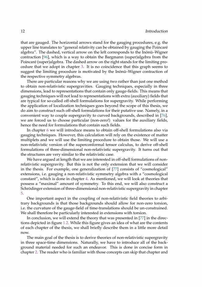
In conclusion, we will extend the theory that was presented in [77] in the direc-tions depicted in figure 1.2. While this figure gives an idea of what are the contentsof each chapter of the thesis, we shall briefly describe them in a little more detailnow.
The main goal of the thesis is to derive theories of non-relativistic supergravityin three space-time dimensions. Naturally, we have to introduce all of the back-ground material needed for such an endeavor. This is done in concise form inchapter 2. The reader who is familiar with those concepts can skip that chapter and

1.3 OUTLINE OF THE THESIS 13
Extensions of Newton–Cartan supergravity considered in this thesis
“original” Newton–Cartan supergravity
off-shell formulation:chapters 3 and 6
“conformal”:chapter 5
non-zero torsion:chapter 6
cosmological:chapter 4
Figure 1.2: Extensions of the “original”, i.e. three-dimensional, N = 2, torsion-less,on-shell, Newton–Cartan supergravity that we consider in this thesis.
immediately proceed to chapters 3–6 where we present the new materials. A quickglance at the summary of the conventions used in this work, presented in section2.1, might be useful.
The chapter on background material, chapter 2, focuses only on the most im-portant points. We introduce the concept of symmetries, gauge symmetries andgauge theories and also present an introduction to general relativity from this pointof view. More importantly, especially for this work, we introduce non-relativisticgravity, supersymmetry and supergravity. The combination of those is the maintheme of our work and makes up the bulk part of the thesis, chapters 3–6. Thechapter is quite technical and we proceed rather quickly to cover all but the neces-sary concepts that we use later on.
The presentation of new material starts in chapter 3, where we develop a non-relativistic contraction/limiting procedure that can be used to derive non-relativ-istic supergravity theories from relativistic ones. After describing the procedure inquite abstract terms, we apply it to some examples. We re-derive Newton–Cartangravity in the formulation in which it appeared earlier in the literature. We willalso comment shortly on why we are mostly concerned with theories with morethan one supersymmetry charge, which are called extended supersymmetries inthe relativistic context. However, we shall argue that those are indeed “minimal” inthe non-relativistic setting. Then we re-derive three-dimensional Newton–Cartansupergravity and we end with a novel off-shell formulation of the latter. Finally,we apply the procedure to derive a non-relativistic version of the superparticle in acurved background. We also comment on the relation of our limiting procedure toother non-relativistic limits that have been put forward in the literature.
A novel non-relativistic supergravity theory is derived in chapter 4. By gaug-ing a particular non-relativistic superalgebra we find a cosmological extension ofNewton–Cartan supergravity, i.e. a generalization of the theory put forward in [77].We will obtain a 1/R-modification of that theory, where R is related to the cosmo-logical constant ΛCC = −1/R2. We keep the same name for the supergravity theorythat we use for the algebra, Newton–Hooke in this case, hence the title Newton–Hooke supergravity. We proceed with a particular choice of gauge-fixing, similar

14 Introduction
to the one performed in [77] to derive 1/R-modifications of Galilean supergravity.3
At the end, we use the procedure of the previous chapter 3, and the new off-shellsupergravity found there, to show that we could have obtained the same results byuse of the limiting procedure.
In chapter 5 we expand on our study of three-dimensional non-relativistic su-pergravities by deriving a “conformal” extension of the non-relativistic supergrav-ities of chapters 3 and 4. This is done, again, by using gauging techniques. Thenon-relativistic algebra that we use in this chapter is a Schrodinger superalgebra.This theory will serve as a base for the “conformal” tensor calculus of the nextchapter.
A non-relativistic version of the superconformal tensor calculus, a “Schrodingertensor calculus”, is introduced in chapter 6. To this end, we first introduce mat-ter multiplets that are coupled to the non-relativistic supergravity background ofchapter 5. These will serve as so-called compensator multiplets in the Schrodingertensor calculus. By gauge-fixing all extra (Schrodinger) symmetries, we derive anoff-shell version of Newton–Cartan supergravity. Because the Schrodinger theoryallows for non-vanishing torsion we are thus able to derive a non-relativistic super-gravity theory with non-zero torsion. We discuss how truncating to zero torsionleads to the theory of chapter 3.
We conclude in chapter 7 and give an outlook on open problems that are not ad-dressed in this thesis and, perhaps more interestingly, those that can be addressedin the future based on the new findings of our work.
3 Galilean supergravity is the supersymmetric extension of Galilean gravity, which by definition isthe non-relativistic theory that is invariant under ’acceleration-extended’ Galilean symmetries.

2Background material
This chapter aims to set the basis for the later chapters. Here we review allphysical theories and principles that will be used later on.
16 CHAPTER 2 BACKGROUND MATERIAL
In this chapter we quickly review the very basics of symmetries, gauge-symmetries,general relativity and supergravity. The purpose is to give a brief introduction to allconcepts that will be needed in later parts of the thesis in an effort to make this workself-contained. Naturally, since there are many textbooks devoted to teach exactlythose subjects, there is too much to say about them. Here, we will proceed at a pacethat cannot do justice to the details and we shall restrict ourselves to features thatwe use in later parts of the thesis.
The expert is likely to know all the material covered in this chapter and mightproceed to the next chapter 3 immediately, possibly after a quick glance over ourconventions in the next section 2.1.
2.1 Conventions
In order to get this technical part out of the way let us devote this first section to abrief overview of the conventions used in this work.
We work mostly in three space-time dimensions, i.e. one time and two spatialdimensions. For the flat Minkowski background we choose the “mostly plus” sig-nature
ηµν = diag(−1, 1, 1) . (2.1)
The first entry is the time-like direction. When we are in more than three dimen-sions a suitable number of (plus) ones must be added.
Greek indices, as in (2.1) are used for curved space-time indices. They run overall coordinates, including time. The spatial subset of such indices is denoted byLatin letters i, j, k, . . . Flat, Lorentz, indices are denoted by Latin indices from thebeginning of the alphabet. In particular, in this thesis we must also differentiatebetween relativistic and non-relativistic indices because in the non-relativistic casewe need to split space and time explicitly. Capital letters usually refer to relativis-tic indices while lowercase letters are again reserved for the spatial part only andusually appear in the non-relativistic context only. An example is given by writingµ = (0, i) and A = (0, a). Using zero for both time-like components of curved andflat indices might cause confusion. However, oftentimes we will simply not writethe zero for flat components, e.g. λa
0 = λa. Then it is important to keep track ofwhere the zero was because a zero up and a zero down differ by a minus sign dueto the metric (2.1).
Symmetrization and anti-symmetrization of indices are denoted with roundand square brackets respectively and we include a normalization factor in the defi-nition, e.g. 2 a[µbν] = aµ bν − aνbµ.
We will come back to spinor and gamma-matrix conventions in section 2.6.Here, let us briefly mention that we will use Majorana spinors and real gamma-
2.2 GAUGE SYMMETRIES 17
matrices given by
γA = (iσ2, σ1, σ3) (2.2)
where σi are the usual Pauli matrices. The charge conjugation matrix C is purelyimaginary
C = iγ0 . (2.3)
Note that numerically γµνρ = εµνρ. This identity holds numerically as γµνρ is ofcourse a matrix while the completely anti-symmetric epsilon symbol is a num-ber. The two-dimensional, purely spatial epsilon symbol is related to the three-dimensional by
ε0ij = εij , ε012 = 1 . (2.4)
We reverse the order of spinors when we do a complex conjugation. Spinor indicesare Greek indices from the beginning of the alphabet and lowercase Latin indiceson spinors are used if there are multiple supercharges Qi.
This ends our short excursion on conventions. Now are ready to dive into the realmof “physics”.
2.2 Gauge symmetriesSymmetries play an immensely important role in this work. Let us introduce themusing a simple example. It is not one that we will need later on in this thesis, itjust serves the purpose of introducing gauge-symmetries. Consider the action of acomplex scalar field Φ(x):
S = −m2
∫d3x ηµν ∂µΦ(x)∂νΦ∗(x) . (2.5)
Never mind the prefactor m/2 or the fact that we chose three-dimensional space-time. This is not important. One more piece of information is that the (inverse)Minkowski metric ηµν which appears in (2.5) is given by the diagonal matrix
ηµν = diag(−1, 1, 1) . (2.6)
This just means that we are in flat space here.
For now the only observation we are interested in is that (2.5) is left invariant ifwe rotate the complex field Φ(x) by an arbitrary phase exp(i α), i.e. we can replacethe field Φ(x) by exp(i α)Φ(x) and this does not alter the form of the action (2.5).
18 CHAPTER 2 BACKGROUND MATERIAL
The infinitesimal version of this transformation is
δΦ(x) = i α Φ(x) , δΦ∗(x) = −i α Φ∗(x) , (2.7)
and those contributions will cancel exactly when we calculate the variation of (2.5).The action is invariant under global U(1) transformations because exp(i α) spanthe group U(1). The transformations are global because the parameter α is constant.If it was not constant the variation of (2.5) would yield additional terms that arisewhen the derivative acts on α.
We can nevertheless modify the action in such a way that the parameter α be-comes a local function of x while still leaving the action invariant. To do so, weneed to introduce a new field Aµ(x) that compensates for the additional contribu-tions that we get from the derivatives acting on α(x). We define a new so-calledcovariant derivative
DµΦ(x) = ∂µΦ(x)− i Aµ(x) , (2.8)
together with a corresponding DµΦ∗(x) for the complex conjugate. Then, if we use
δAµ(x) = ∂µα(x) , (2.9)
we note that the quantity (2.8) transforms just like the field Φ(x), i.e. its transfor-mation is given by δDµΦ(x) = iα DµΦ(x). The gauge-field Aµ(x) is added pre-cisely for that purpose, to cancel the derivative of the parameter α(x). This way wegauged our first symmetry. The field Aµ(x) is the gauge-field for the (local U(1)gauge) symmetry Φ(x)→ exp[i α(x)]Φ(x).
Note that there is no covariant derivative of Aµ(x) because it already trans-forms with the derivative of the parameter. Taking this thought a little bit furtherwe realize that gauge-fields must always be part of some covariant expression, likethe covariant derivative that we just introduced, or a curvature which we will intro-duce below. A gauge-field cannot “stand alone” as it would not lead to an invariantor covariant expression.
The symmetry here is U(1) because α(x) is just a number. If we think of this asan identity times the parameter α(x) we can also envision generalizing this to othergroups where we have several α(x)s labeled by α(x)a multiplying some matricesTa. This is, in very short terms, how other transformations, such as for examplerotations, work.
For any field such as Φ(x) or Aµ(x) and their symmetry transformations wecan define quantities that are invariant or covariant under those symmetry trans-formations. The first such quantity was the covariant derivative introduced in (2.8).Another very important quantity is the curvature of the gauge-field. In our presentcase, it is given by
Fµν(A) = ∂µ Aν(x)− ∂ν Aµ(x) = 2 ∂[µ Aν](x) . (2.10)

2.2 GAUGE SYMMETRIES 19
Curvatures are always invariant under the gauge-transformation of the respectivegauge-fields but they transform covariantly under all other transformations of thefield. (For example Fµν(A) is invariant under transformations with parameter α(x)but it does transform like a covariant two tensor under diffeomorphisms.)
We can write down a dynamical theory for the gauge-field Aµ(x) by makinguse of the curvature (2.10). The action
S = −14
∫d3x ηµνηρσ Fµρ(A) Fνσ(A) (2.11)
can be used for that purpose. Much like (2.5) (using covariant derivatives) it issecond order in derivatives and also invariant under the U(1) symmetry transfor-mations.
The actions (2.5) and (2.11) are examples of the few actions that we will intro-duce in this chapter. The main reason is that, while actions exist for “relativistic”gravity, no such action exists for the non-relativistic gravitational theories that wewill use and hence we mostly work without actions. We will come back to this pointin chapter 3. Indeed, we would like to stress that there is no need for an action todescribe a theory, usually transformation rules and possibly equations of motionsuffice. Having an action however, simply reduces the amount of information thatis needed as transformation rules and equations of motion can always be deducedfrom the action.
In the following we will always use the infinitesimal version of the symmetrytransformations, for example (2.7) instead of Φ(x) → exp[i α(x)]Φ(x) and we willin general not denote the dependence of gauge-fields and parameters on the coor-dinates. Unless stated otherwise, we will assume that they are all functions of thespace-time coordinates xµ.
In summary, all (gauge) theories that we will deal with later on will be given interms of their field content, e.g. Aµ, the transformations of the fields under all sym-metries, e.g. (2.9), and possibly some additional constraints on the fields, which areusually constraints on the curvatures. For example, using the definition of Fµν(A)we see that
∂[µFνρ](A) = 0 . (2.12)
We noted earlier that there is no covariant derivative for Aµ, so we are inclined togeneralize (2.12) to the—indeed correct and very powerful—statement that
D[µFνρ](A) = 0 . (2.13)
This is know as the Bianchi identity. It says that the totally anti-symmetrized co-variant derivative of any curvature must vanish.
Another constraint on Fµν(A), and thus on Aµ, can be derived from the action
20 CHAPTER 2 BACKGROUND MATERIAL
(2.11). It is the equation of motion for Aµ given by
ηµν∂µFνρ(A) = 0 . (2.14)
As we will not always have the luxury of an action we do not immediately knowwhich constraints are really equations of motion and which ones follow for exam-ple from Bianchi identities or are imposed by hand. There might be a way to findout, however. The constraints transform under symmetry transformations like thecurvatures themselves. Equations of motion always transform to equations of mo-tion and likewise for other constraints. If we know one equation of motion we canalways derive other ones by symmetry variations.
The main aim of this chapter is to introduce yet another gauge-theory that willturn out to be nothing else but the theory of general relativity. Having done so, wewill also be able to couple the scalar and vector theories of this section to a curvedbackground. Before doing so, we shortly digress and talk about the symmetry al-gebras that underly our gauge-theories.
2.3 Symmetry algebras
We should shortly comment on how algebras link to everything we heard so far.Remember the theory of the last section was a U(1) theory because α was just anumber. We thought about replacing it with several αs that multiply matrices Ta.Now, those matrices Ta will (in general) not commute, but their commutation rela-tions will form an algebra.
A well-known theorem by Emmy Nother dictates that for every symmetry whichleaves a given theory invariant there exists a conserved current. This current givesrise to a quantity called the generator of the symmetry. Oftentimes these operatorsare “scalar quantities”, e.g. differential operators, sometimes, as we alluded to be-fore, they can be written as matrices. If the generators of the symmetries of a giventheory do not commute, we say that the non-vanishing commutation relations ofthose symmetry generators form the symmetry algebra of the theory.
We will always denote symmetry algebras using commutation relations. How-ever, this is only for notational purposes, we do not imply any quantization of thetheory. Equivalently, we could use Poisson brackets everywhere.
An example of such an algebra, that we will also use in the next section, is thePoincare algebra. Its non-vanishing commutation relations are[
PA, MBC]= 2 ηA[B PC] ,
[MAB, MCD
]= 4 η[A[C MD]B] . (2.15)
Note, that in contrast to the standard literature we prefer representations that donot have too many i’s. All our generators, PA for translations and MAB for rota-tions, are anti-hermitian operators. In particular, this means that an infinitesimal
2.4 GAUGING THE POINCARE ALGEBRA 21
transformation is given by, e.g.
δ• = ζA PA • . (2.16)
The bullet shall denote an arbitrary field in our theory. The finite transformationis given by the exponential of this expression. Compare e.g. to exp(i I α)Φ, wherethe “generator” I (the identity) is real and we have an explicit factor of i such thatthe hermitian conjugate of exp(i I α) gives the inverse transform. We will not havethose i’s in the algebra, nor in the finite transformation.
2.4 Gauging the Poincare algebraIn this section we will show how the vielbein formulation of general relativity canbe seen as a gauge-theory of the Poincare algebra. In the following we will “gauge”the algebra (2.15). This exercise is done in many textbooks on general relativityand/or supergravity. It will serve as an important basis for us, first to comparewith results that we will derive later on, and secondly for the gauging of the non-relativistic Newton–Hooke superalgebra which we will perform in chapter 4, aswell as the Schrodinger algebra in chapter 5.
The first step in the gauging procedure is to assign a gauge-field to every gen-erator of the algebra. From (2.16) one can derive very general rules that determinehow those gauge-fields must transform in terms of the structure constants of thesymmetry algebra, see e.g. [97]. In particular, we define a connection Aµ that takesvalues in the adjoint of the gauge group. For the Poincare algebra we choose
Aµ = EµA PA +
12
ΩµAB MAB , (2.17)
where EµA and Ωµ
AB will eventually take over the roles of the relativistic vielbeinand spin-connection. We can then realize the algebra on Aµ using the transforma-tion rule
δAµ = ∂µζ +[Aµ, ζ
], (2.18)
where the gauge-parameter ζ is given by
ζ = ζA PA +12
λAB MAB . (2.19)
This leads to the following transformations of the relativistic vielbein EµA and the
spin-connection ΩµAB:
δEµA = ∂µζA −Ωµ
ABζB + λAB Eµ
B , (2.20)
δΩµAB = ∂µλAB + 2 λ[A
C ΩµCB] . (2.21)
22 CHAPTER 2 BACKGROUND MATERIAL
In a similar manner we define curvatures
Rµν(A) = 2 ∂[µAν] +[Aµ,Aν
]= Rµν
A(E) PA +12
RµνAB(Ω) MAB , (2.22)
and find
RµνA(E) = 2 ∂[µEν]
A − 2 Ω[µA
B Eν]B , (2.23)
RµνAB(Ω) = 2 ∂[µΩν]
AB − 2 Ω[µA
C Ων]CB . (2.24)
The connection Aµ is a vector and also transforms in the usual way under generalcoordinate transformations:
δAµ = ξρ∂ρAµ +Aρ∂µξρ = LξAµ . (2.25)
From (2.18) and (2.25) we can define a new transformation, using the symmetryparameter
Σ = Λ− ξµAµ . (2.26)
Unlike Λ though, Σ only takes values in the internal/homogeneous part of thesymmetry group. In the present case, this means
Σ =12
λAB MAB , (2.27)
and it leads to the following general transformation
δAµ = δAµ − ξνRµν(A) = Lξ + ∂µΣ +[Aµ, Σ
]. (2.28)
Those are exactly the transformations that we are interested in. All fields will trans-form as vectors under general coordinate transformations and keep their originalsymmetry transformations under the internal symmetries.
This is slightly different for supersymmetry. There, we would like to replaceonly local translations by diffeomorphisms, but not the supersymmetry transfor-mations. Thus Σ will consist of the homogeneous part plus supersymmetry. This isnot straightforward though because the anti-commutator of two supersymmetriesleads to a local translation, hence two “ordinary” symmetries lead to one that wereplaced by (2.28). The result is that the anti-commutators of supercharges will takevery peculiar forms and for most theories that we consider in this thesis we will beparticularly interested in the closure of the algebra of those anti-commutators. Forthe time being let us focus on the bosonic problem.
While it is not strictly necessary to do so, one would oftentimes like to identifythe transformations (2.18) and (2.28). For example, we will make this identificationfor all bosonic theories. Then it is useful to set the curvature of the independent
2.4 GAUGING THE POINCARE ALGEBRA 23
gauge-fields, in this case only EµA, to zero:
RµνA(E) = 0 . (2.29)
On the one hand, this removes the curvature contributions to the formula (2.28),thus enabling us to identify local translations with general coordinate transforma-tions. On the other hand, it allows us to solve for the spin-connection Ωµ
AB(E) interms of Eµ
A:
ΩµAB(E) = −2 Eρ[A∂[µEρ]
B] + EµCEρAEνB∂[ρEν]C . (2.30)
From now on we shall always assume that the spin-connection is a dependent fieldthat is given in terms of the independent gauge-fields through the solution of a(curvature) constraint such as (2.29). This also brings us closer to the theory ofgeneral relativity as there is no independent spin-connection in that theory either.Now, the transformation of the vielbein follows from (2.28) and it is given by
δEµA = ξρ∂ρEµ
A + EρA∂µξρ + λA
BEµB . (2.31)
The transformation of ΩµAB(E) follows from its expression in term of Eµ
A andusing (2.31). In the case at hand, it is still given by (2.21) for local Lorentz rotations.It also transforms under diffeomorphisms in the usual way, i.e.
δΩµAB(E) = ξρ∂ρΩµ
AB + ΩρAB∂µξρ + ∂µλAB + 2 λ[A
C ΩµCB] . (2.32)
This finishes the gauging procedure. We have obtained the kinematics of generalrelativity. In a next step, we will impose equations of motion on the only indepen-dent field left, the vielbein Eµ
A. Before doing so we digress shortly for a remarkon the nature of the transformations under general coordinate transformations. In-deed, the first two terms in (2.31) and (2.32) are the transformation of a covarianttensor under general coordinate transformations. It is the infinitesimal version, us-ing the transformation δxα = ξα, of the defining law
Tµ
(xν)=
∂xα
∂xµ Tα
(xβ)
, (2.33)
for a covariant tensor. Two-tensors such as the metric (2.36) transform with two fac-tors ∂x/∂x and any contravariant (upper) index transforms with an inverse factor∂x/∂x.
Putting the torsion to zero also implies that the relativistic curvature (2.24) iden-tically satisfies the Bianchi identity
R[µνρ]B(Ω) = R[µν
AB(Ω) Eρ]A = 0 , (2.34)
which follows from (2.13) and the transformation of EµA given in (2.20).
24 CHAPTER 2 BACKGROUND MATERIAL
Finally, we can put the theory on-shell by imposing yet another constraint onthe curvature, the Einstein equation. In the current formulation, it reads
EµA Rµν
AB(Ω) = 0 , (2.35)
where ΩµAB(E) is expressed in terms of Eµ
A using (2.30).In chapter 3 we will consider the non-relativistic limit of the formulas (2.20)–
(2.35) that we collected here.
To put field theories such as the scalar or vector of section 2.2 in a curved back-ground we have to introduce one more connection. In the same way that we intro-duced Aµ to cancel the derivative of the parameter α we need a new (in this casedependent) field that deals with derivatives of the parameter of diffeomorphisms,such that we have a derivative ∇µ that is covariant with respect to general coordi-nate transformations. This Christoffel connection can be defined by requiring thatthe covariant derivative of the vielbein, and by extension of the metric, given by
gµν = ηABEµAEν
B , (2.36)
is zero. Eta is again the Minkowski metric (2.1), hence all Latin indices are flatindices while Greek indices are curved space-time indices. If the vielbein is just adelta function then the space-time is flat.
The equivalence principle of general relativity states that we are always able togo to a flat frame locally. The vielbeins are doing exactly this. We will see laterthat the introduction of vielbeins is an immense simplification when working withspinors, as it is much easier to work with spinors and gamma-matrices in flat space.
Coming back to the connection we define it by
∇µEνA = 0 = DµEν
A − ΓρµνEρ
A . (2.37)
Here Dµ is the covariant derivative with respect to the transformations given bythe algebra and we solve (2.8) by
Γρµν(E) = Eρ
ADµEνA . (2.38)
Now the curved space analogues of (2.5) and (2.11) are given by writing aninvariant measure for the integral
d3x → d3x det(EµA) , (2.39)
replacing the (inverse) Minkowski metric by the curved (inverse) metric
ηµν → gµν , (2.40)
2.5 NON-RELATIVISTIC GRAVITY 25
and replacing all partial derivatives with covariant ones
∂µ → ∇µ . (2.41)
These substitutions suffice to put any theory in a curved background.
Finally, let us connect our theory of general relativity, as we presented it here, to theform that one usually finds in textbooks. In fact, we have derived gravity in whatis referred to as the second order formulation of general relativity. Normally, oneintroduces the metric (2.36), the covariant derivative ∇µ with the Christoffel con-nection (2.38), and the Riemann tensor (2.24). Further contractions of the Riemanntensor are the Ricci tensor given in (2.35), which still has to vanish on-shell, and theRicci scalar
R(Ω) = EµAEν
B RµνAB(Ω) . (2.42)
The Einstein–Hilbert action of general relativity in D space-time dimensions is thengiven by
S = − 1κ2
∫dDx det(Eµ
A) R(Ω) . (2.43)
The equation of motion for the only independent field EµA, or the metric (2.36),
is the Einstein equation (2.35). The term “second order formulation” refers to thefact that the action (2.43) is second order in derivatives and that Eµ
A is the onlyindependent field.
This finishes our discussion of “relativistic” gravity. In the next section webriefly describe some notions of non-relativistic gravity with different amount ofsymmetries.
2.5 Non-relativistic gravityAs we briefly pointed out in the introduction, there are different theories of non-relativistic gravity. The difference lies only in the amount of symmetry that weallow. In this thesis, we refer to Newtonian gravity for a system that is in fact notsubject to any gravitational force, i.e. a free-falling frame. Obviously, the symmetrytransformations that related different such frames are the Galilei transformations.Galilean gravity, see 2.5.1, is the first generalizations of such a system. There, weallow for arbitrary time-dependent spatial translations, and the gravitational forceis determined by a Newton potential Φ. The fully gauged version, where we al-low for arbitrary coordinate transformations is Newton–Cartan gravity, see 2.5.2,and the gravitational fields are (τµ, eµ
a, mµ). In the subsections 2.5.3 and 2.5.4 wecomment on some issues that are related to the dynamics of non-relativistic grav-ity theories and the non-relativistic limit of gravity in three space-time dimensions,respectively.

26 CHAPTER 2 BACKGROUND MATERIAL
2.5.1 Galilean gravityHere any gravitational attraction is governed by the Newton potential Φ(x) only.This Newton potential is subject to the Laplace equation,
∂i∂iΦ(x) = 0 . (2.44)
We will see later on, in chapter 4, that we should interpret (2.44) as the equation ofmotion for a “flat space” Newton potential, as opposed to the Galilean version ofNewton–Hooke gravity.
A theory is non-relativistic if it is invariant under Galilei transformations, i.e. itssymmetry algebra is the Galilei algebra. Its non-vanishing commutators are givenby [
Pa, Jbc]= 2 δa[b Pc] ,
[Jab, Jcd
]= 4 δ[a[c Jd]b] ,[
Ga, Jbc]= 2 δa[b Gc] ,
[H, Ga
]= Pa ,
(2.45)
where H, Pa, Ga and Jab are the generators of time- and space-translations, boostsand rotations, respectively. The Galilei algebra admits a central extension [98],i.e. we can add one more generator Z that commutes with all other generators.It would appear in the following commutator[
Pa, Gb]= δab Z . (2.46)
In the following subsection, we will give some more reasons for our use of thiscentral extension. The centrally extended Galilei algebra is usually called the Barg-mann algebra. We will also adopt this nomenclature and from now on we aremostly concerned with this centrally extended version of the Galilei algebra. Note,the three-dimensional Galilei or Bargmann algebra also admits another central ex-tension, see e.g. [99]. With generalizations to higher dimensions in mind we willnot consider that extension in this work.
Using the argument that a non-relativistic theory must be in variant under theGalilei or Bargmann algebra, and with the gauge-theory description of general rel-ativity in mind, we will come to the conclusion that non-relativistic gravity couldalso be a gauge-theory of non-relativistic diffeomorphisms, i.e. a gauged version ofthe Galilei or Bargmann algebra. This is exactly the way Newton–Cartan gravitywas derived in [80]. We shall come back to this point later.
Let us now consider un-gauged representations of non-relativistic algebras. Wecan write down a representation of the Bargmann algebra using a single scalar φ(note that this φ is not the Newton potential) in the same way as (2.20) and (2.21)are a representation of the Poincare algebra (2.15). We would use
δφ = ζ∂tφ + ξ i∂iφ− λijxj∂iφ + tλi∂iφ + m λixiφ + m σ φ . (2.47)
The constant parameters ζ, ξ i, λi, λij and σ are for time- and space-translations,
2.5 NON-RELATIVISTIC GRAVITY 27
boosts, rotations and central charge transformations. The parameter m here is amass parameter and for m → 0 (2.47) realizes the Galilei algebra. This is one wayto see that the Bargmann algebra is connected to massive representations.
Note, the transformation rules of the Newton potential are not given by (2.47),see (2.48) below.
This far we are in what we will later refer to as (non-relativistic) “flat space”. Itis characterized by the fact that the underlying symmetry algebra is given by theGalilei algebra (2.45). In particular, only constant translations ξ i are allowed. Wecould consider a partial gauging of the Galilei or Bargmann algebra—a full gaugingwould of course lead to Newton–Cartan gravity [80]—such that we allow for arbi-trary time-dependent translations ξ i(t). In this case the symmetry algebra is notthe Galilei algebra anymore but we will speak of “acceleration-extended Galilei”,or Milne [4], symmetries and we are in a “curved” background that is characterizedby the Newton potential Φ [100].
The transformation of this Newton potential is given by [77, 101]
δΦ = ζ∂tΦ + ξ i(t) ∂iΦ− λijxj∂iΦ + ∂t∂tξ
i(t) xi + m σ(t)Φ . (2.48)
Note the difference to the transformation of an arbitrary scalar field, the gaugedversion of (2.47),
δφ = ζ∂tφ + ξ i(t) ∂iφ− λijxj∂iφ + m ∂tξ
i(t) xiφ + m σ(t) φ . (2.49)
It is obvious that the Newton potential is not a normal scalar field. The ∂t∂tξi(t)xi
term reminds us of its (gravitational) spin-two origin. This term survives the m →0 limit, which eliminates the central charge transformations σ(t) (which are alsogauged with respect to the Bargmann transformation (2.47) where σ is a constant).
2.5.2 Newton–Cartan gravityAnother, more general formulation of non-relativistic gravity is due to Cartan [2,3].This so-called Newton–Cartan theory is a reformulation of Newtonian gravity thatis invariant under general coordinate transformations, i.e. local transformations,not only constant ones like in (2.47). We shall not describe that theory in too muchdetail here as we are essentially going to re-derive it in chapter 3 by taking a non-relativistic limit of general relativity.
Let us mention that one can obtain this Newton–Cartan theory in the same wayas we obtained general relativity in the previous section, by gauging the underlyingsymmetry algebra. In the case of Newton–Cartan gravity one needs to gauge theBargmann algebra. This was done in [80]. Similar techniques were used to derive anon-relativistic supergravity theory in [77] and we will also use such techniques toderive Newton–Hooke supergravity in chapter 4 and Schrodinger supergravity inchapter 5.
The reasons for using the Bargmann algebra are the following. On a technicallevel, the addition of the central charge gauge-field mµ and its related curvature
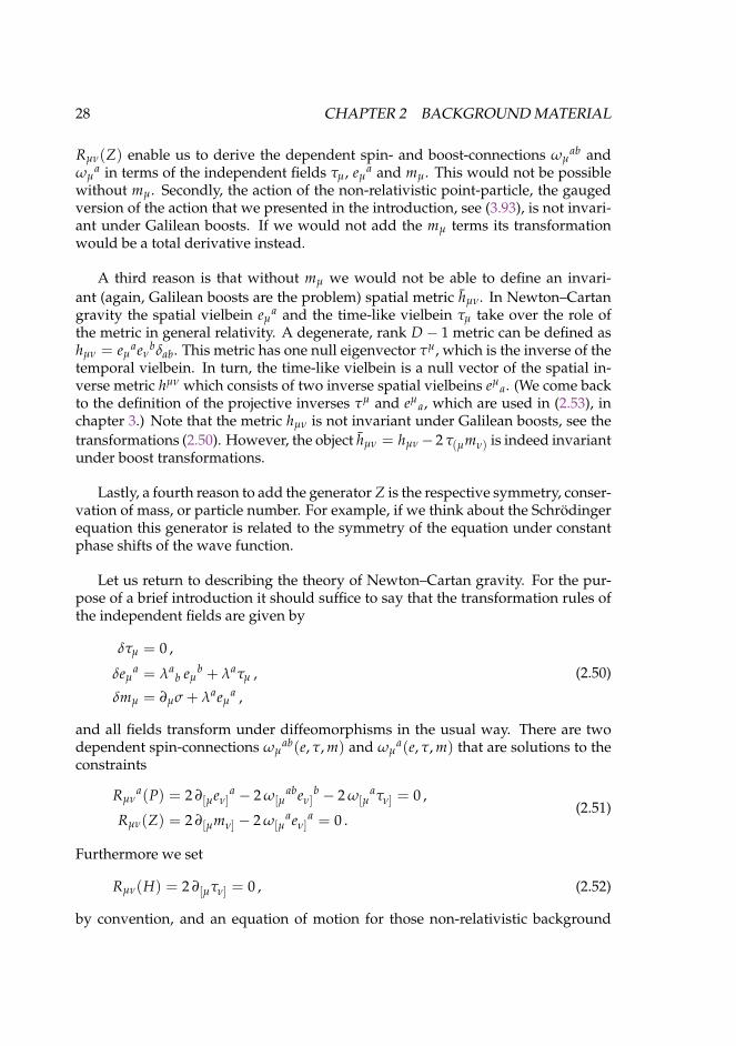
28 CHAPTER 2 BACKGROUND MATERIAL
Rµν(Z) enable us to derive the dependent spin- and boost-connections ωµab and
ωµa in terms of the independent fields τµ, eµ
a and mµ. This would not be possiblewithout mµ. Secondly, the action of the non-relativistic point-particle, the gaugedversion of the action that we presented in the introduction, see (3.93), is not invari-ant under Galilean boosts. If we would not add the mµ terms its transformationwould be a total derivative instead.
A third reason is that without mµ we would not be able to define an invari-ant (again, Galilean boosts are the problem) spatial metric hµν. In Newton–Cartangravity the spatial vielbein eµ
a and the time-like vielbein τµ take over the role ofthe metric in general relativity. A degenerate, rank D− 1 metric can be defined ashµν = eµ
aeνbδab. This metric has one null eigenvector τµ, which is the inverse of the
temporal vielbein. In turn, the time-like vielbein is a null vector of the spatial in-verse metric hµν which consists of two inverse spatial vielbeins eµ
a. (We come backto the definition of the projective inverses τµ and eµ
a, which are used in (2.53), inchapter 3.) Note that the metric hµν is not invariant under Galilean boosts, see thetransformations (2.50). However, the object hµν = hµν− 2 τ(µmν) is indeed invariantunder boost transformations.
Lastly, a fourth reason to add the generator Z is the respective symmetry, conser-vation of mass, or particle number. For example, if we think about the Schrodingerequation this generator is related to the symmetry of the equation under constantphase shifts of the wave function.
Let us return to describing the theory of Newton–Cartan gravity. For the pur-pose of a brief introduction it should suffice to say that the transformation rules ofthe independent fields are given by
δτµ = 0 ,
δeµa = λa
b eµb + λaτµ ,
δmµ = ∂µσ + λaeµa ,
(2.50)
and all fields transform under diffeomorphisms in the usual way. There are twodependent spin-connections ωµ
ab(e, τ, m) and ωµa(e, τ, m) that are solutions to the
constraints
Rµνa(P) = 2 ∂[µeν]
a − 2 ω[µabeν]
b − 2 ω[µaτν] = 0 ,
Rµν(Z) = 2 ∂[µmν] − 2 ω[µaeν]
a = 0 .(2.51)
Furthermore we set
Rµν(H) = 2 ∂[µτν] = 0 , (2.52)
by convention, and an equation of motion for those non-relativistic background

2.5 NON-RELATIVISTIC GRAVITY 29
fields is given by the trace of the curvature of Lorentz boosts
τµeνaRµν
a(G) = R0aa(G) = 0 . (2.53)
Furthermore, there are more constraints on the curvatures Rµνab(J) and Rµν
a(G)that follow from the Bianchi identities.
Note that the constraint (2.52) implies that the theory has no torsion. General-izations of Newton–Cartan gravity with torsion are given in [25–29].
As a final remark for this very short summary on Newton–Cartan gravity letus mention that one can obtain the formulas for the acceleration-extended Galileitheory through a particular gauge-fixing of the Newton–Cartan theory. This wasshown in [77] and we will use the same gauge-fixing to get a Galilean version ofNewton–Hooke supergravity in chapter 4. This gauge-fixing offers a clear way tosee how the Newton potential is related to the background fields of the Newton–Cartan theory.
2.5.3 Non-trivial dynamicsAnother, not yet fully understood point is related to the dynamics of Newton–Cartan gravity. On the one side, [77,80] gives equations of motion for the Newton–Cartan fields for “flat” space-times, i.e. space-times for which the curvature of spa-tial rotations vanishes Rµν
ab(J) = 0. It is, at the time of the writing of this thesis,currently under investigation how this must be generalized for curved space-times,i.e. space-times were Rµν
ab(J) 6= 0, see [102]. On the other side there are proposalsfor dynamics determined by an action [103], see also [20]. In particular it is arguedthat the action for Newton–Cartan gravity is given by (extended) Horava–Lifshitzgravity [104, 105]. However, it remains to check if these actions indeed give rise tothe same equations of motion that are given in [102] or [77, 80].
For more details we must refer the reader to [102]. However, let us make someintriguing remarks about why it is so difficult to describe dynamics for the Newton–Cartan background fields. It was shown in [77, 80] that Newton–Cartan gravity isultimately related to the Bargmann algebra, rather than the Galilei algebra. Thedifference is that the Bargmann algebra allows for one more symmetry genera-tor Z, i.e. one more symmetry that the equations of motion have to obey. OnceRµν
ab(J) 6= 0 the equations of motion that were proposed in [77, 80] are not any-more invariant under Galilean boosts. This problem can be solved by adding ex-tra terms, proportional to Rµν
ab(J) times mµ, the gauge-field of the central chargesymmetry Z. The drawback is that these new equations of motion are not invari-ant under central charge transformations anymore. Moreover, without introducingnew fields one cannot overcome this problem. So, either one adds a Stuckelbergfield [102], see also [29], or the equations of motion are not invariant under centralcharge symmetry. One is always free to opt for the first option, but we would liketo point out an interesting fact about the second one.
The central charge symmetry is related to the conservation of the particle num-
30 CHAPTER 2 BACKGROUND MATERIAL
ber. Thus, if the equations of motion are not invariant under Z it would mean thatin non-relativistic curved space-times the total number of particles is not conserved.But this should not come as a big surprise given that we know that this is certainlythe case for some relativistic curved space-times. Indeed, in de Sitter space-times,which are space-times with a non-vanishing positive cosmological constant, wecannot define a unique vacuum, see e.g. [106], and particle number is certainly notconserved when we are able to create particles simply by choosing a new vacuumstate.
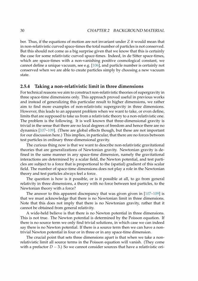
2.5.4 Taking a non-relativistic limit in three dimensionsFor technical reasons we aim to construct non-relativistic theories of supergravity inthree space-time dimensions only. This approach proved useful in previous worksand instead of generalizing this particular result to higher dimensions, we ratheraim to find more examples of non-relativistic supergravity in three dimensions.However, this leads to an apparent problem when we want to take, or even define,limits that are supposed to take us from a relativistic theory to a non-relativistic one.The problem is the following. It is well known that three-dimensional gravity istrivial in the sense that there are no local degrees of freedom and hence there are nodynamics [107–109]. (There are global effects though, but these are not importantfor our discussion here.) This implies, in particular, that there are no forces betweentest particles in ordinary three-dimensional gravity.
The curious thing now is that we want to describe non-relativistic gravitationaltheories that are generalizations of Newtonian gravity. Newtonian gravity is de-fined in the same manner in any space-time dimension, namely the gravitationalinteractions are determined by a scalar field, the Newton potential, and test parti-cles are subject to a force that is proportional to the (spatial) gradient of this scalarfield. The number of space-time dimensions does not play a role in the Newtoniantheory and test particles always feel a force.
The question is how is it possible, or is it possible at all, to go from generalrelativity in three dimensions, a theory with no force between test particles, to theNewtonian theory with a force?
The answer to this apparent discrepancy that was given given in [107–109] isthat we must acknowledge that there is no Newtonian limit in three dimensions.Note that this does not imply that there is no Newtonian gravity, rather that itcannot be obtained from general relativity.
A wide-held believe is that there is no Newton potential in three dimensions.This is not true. The Newton potential is determined by the Poisson equation. Ifthere is no source term we only find trivial solutions, in which case we can indeedsay there is no Newton potential. If there is a source term then we can have a non-trivial Newton potential in four or in three or in any space-time dimension.
The crucial point that sets three dimensions apart is that when we take a non-relativistic limit all source terms in the Poisson equation will vanish. (They comewith a prefactor D− 3.) So we cannot consider sources that have a relativistic ori-
2.6 SPINORS 31
gin. But if we forget, or do not require a relativistic origin of the source, we cansimply add it by hand and we can find non-trivial solutions to the Poisson equa-tion also in three space-time dimensions.
This does not pose any problems to us if we try do construct non-relativisticsupergravity theories from scratch because in this scenario we don’t think aboutconnections to the relativistic theory. But it is confusing in view of the limitingprocedure that we adopt in chapter 3. This procedure does seem to yield Newton–Cartan gravity as some sort of limit of general relativity, for any space-time dimen-sion. Nevertheless, also in this case we obtain the correct equation of motion inthree dimensions (mainly because we derive a source free equation).
This completes our discussion of symmetries and relativistic and non-relativisticgravitational backgrounds, for the bosonic case. We already saw in the transfor-mation rule (2.20) that symmetries might link different fields of the theory, albeitthis is not true anymore in the equations that we will use (2.31). In the following,we will introduce a new symmetry that must, due to its very nature, mix fields ofdifferent spin, hence different fields. But first we shall take a small detour and talkmore about spin and what spinors are.
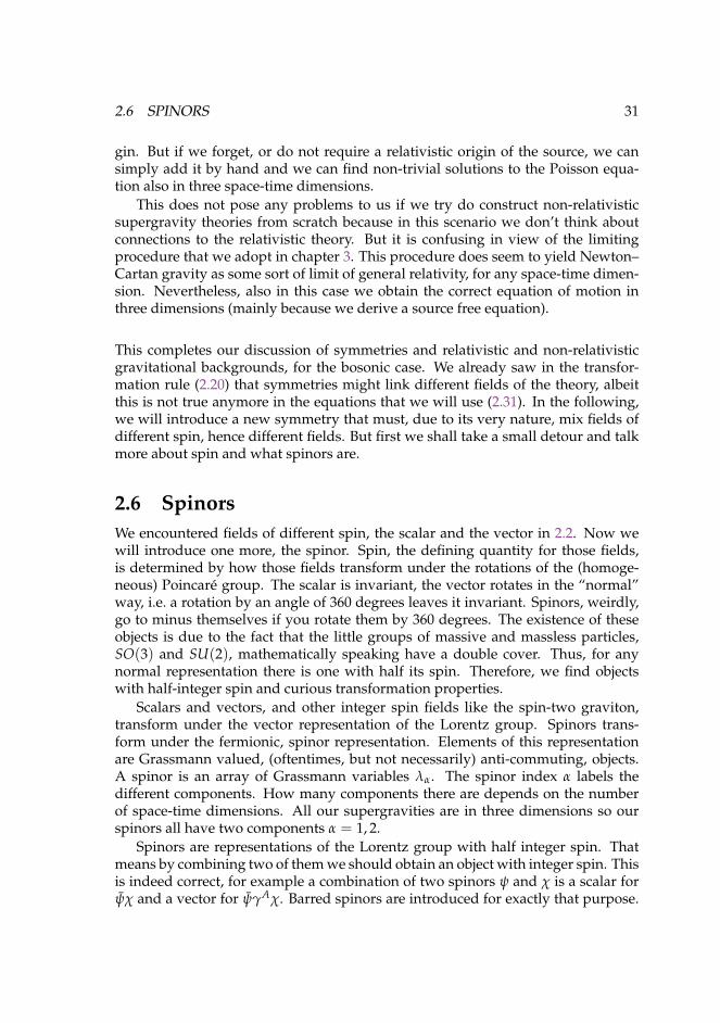
2.6 SpinorsWe encountered fields of different spin, the scalar and the vector in 2.2. Now wewill introduce one more, the spinor. Spin, the defining quantity for those fields,is determined by how those fields transform under the rotations of the (homoge-neous) Poincare group. The scalar is invariant, the vector rotates in the “normal”way, i.e. a rotation by an angle of 360 degrees leaves it invariant. Spinors, weirdly,go to minus themselves if you rotate them by 360 degrees. The existence of theseobjects is due to the fact that the little groups of massive and massless particles,SO(3) and SU(2), mathematically speaking have a double cover. Thus, for anynormal representation there is one with half its spin. Therefore, we find objectswith half-integer spin and curious transformation properties.
Scalars and vectors, and other integer spin fields like the spin-two graviton,transform under the vector representation of the Lorentz group. Spinors trans-form under the fermionic, spinor representation. Elements of this representationare Grassmann valued, (oftentimes, but not necessarily) anti-commuting, objects.A spinor is an array of Grassmann variables λα. The spinor index α labels thedifferent components. How many components there are depends on the numberof space-time dimensions. All our supergravities are in three dimensions so ourspinors all have two components α = 1, 2.
Spinors are representations of the Lorentz group with half integer spin. Thatmeans by combining two of them we should obtain an object with integer spin. Thisis indeed correct, for example a combination of two spinors ψ and χ is a scalar forψχ and a vector for ψγAχ. Barred spinors are introduced for exactly that purpose.
32 CHAPTER 2 BACKGROUND MATERIAL
The index A on the gamma-matrix is the vector index of the (Lorentz) vector VA =ψγAχ.
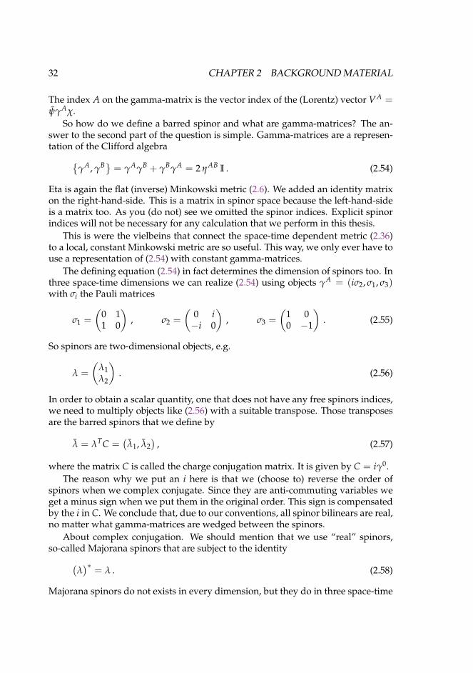
So how do we define a barred spinor and what are gamma-matrices? The an-swer to the second part of the question is simple. Gamma-matrices are a represen-tation of the Clifford algebra
γA, γB = γAγB + γBγA = 2 ηAB I . (2.54)
Eta is again the flat (inverse) Minkowski metric (2.6). We added an identity matrixon the right-hand-side. This is a matrix in spinor space because the left-hand-sideis a matrix too. As you (do not) see we omitted the spinor indices. Explicit spinorindices will not be necessary for any calculation that we perform in this thesis.
This is were the vielbeins that connect the space-time dependent metric (2.36)to a local, constant Minkowski metric are so useful. This way, we only ever have touse a representation of (2.54) with constant gamma-matrices.
The defining equation (2.54) in fact determines the dimension of spinors too. Inthree space-time dimensions we can realize (2.54) using objects γA = (iσ2, σ1, σ3)with σi the Pauli matrices
σ1 =
(0 11 0
), σ2 =
(0 i−i 0
), σ3 =
(1 00 −1
). (2.55)
So spinors are two-dimensional objects, e.g.
λ =
(λ1λ2
). (2.56)
In order to obtain a scalar quantity, one that does not have any free spinors indices,we need to multiply objects like (2.56) with a suitable transpose. Those transposesare the barred spinors that we define by
λ = λTC =(λ1, λ2
), (2.57)
where the matrix C is called the charge conjugation matrix. It is given by C = iγ0.The reason why we put an i here is that we (choose to) reverse the order of
spinors when we complex conjugate. Since they are anti-commuting variables weget a minus sign when we put them in the original order. This sign is compensatedby the i in C. We conclude that, due to our conventions, all spinor bilinears are real,no matter what gamma-matrices are wedged between the spinors.
About complex conjugation. We should mention that we use “real” spinors,so-called Majorana spinors that are subject to the identity(
λ)∗
= λ . (2.58)
Majorana spinors do not exists in every dimension, but they do in three space-time
2.6 SPINORS 33
dimensions so we make use of that. If we would use for example Dirac spinors,then bilinears would be complex numbers and our previous statement about thembeing real would not hold. It follows that Majorana spinors have half as manydegrees of freedom as Dirac spinors.
Because we use Majorana spinors it makes sense to consider the transpose of aspinor bilinear. The transpose of the gamma-matrices and of C follows from theirrepresentation through the Pauli matrices. They can be written as
CT = −C ,(γA)T
= −CγAC−1 , (2.59)
which holds for any representation, not just for ours. Using (2.59) we can show forexample that
ψχ = χψ , ψγAχ = −χγAψ . (2.60)
What if we have two spinors, a barred and a normal one that are not contracted?Can we write them in terms of bilinears? We certainly can. Two spinors that arenot contracted essentially give rise to a quantity with two free indices in spinorspace, i.e. a matrix in spinor space. Such a matrix consists of four independententries, hence we need four independent basis elements to determine it. Thosefour independent elements are readily found by the identity plus the three Paulimatrices or the three gamma-matrices γA. The completeness relation, also calledFierz identity, in three dimensions is given by
χψ =12
ψχ I− 12
ψγAχ γA . (2.61)
This ends the rather technical discussion on properties of spinors and how to ma-nipulate when doing calculations.
Finally, let us come back to our starting point, the transformation of spinors underLorentz rotations. This is given by
δψ =14
λABγABψ . (2.62)
We use γAB = (γAγB − γBγA)/2. Any object that transforms under a rotation inthis manner is a spinor and we can use (2.62) to show that any spinor-bilinear is aboson, a scalar, a vector or a spin-two field.
This concludes our short excursion on relativistic spinors and some of theircharacteristics. As this thesis deals with non-relativistic supergravity, we will ofcourse encounter non-relativistic spinors. Let us anticipate here what the non-relativistic analog of (2.62) will be. In (2.62) the indices A and B run over all space-and time-components. In the non-relativistic case, we will differentiate between
34 CHAPTER 2 BACKGROUND MATERIAL
them. Hence we will find
δψ =14
λabγabψ , (2.63)
if the representation contains only one spinor variable. Since we will mostly dealwith so-called extended supersymmetry, we will in general have at least two spino-rial objects, which will generically transform as
δψ1 =14
λabγabψ1 ,
δψ2 =14
λabγabψ2 −12
λaγa0ψ1 .(2.64)
We will come across many representations of this form in chapters 3–6 wheneverthere are at least two spinors in the multiplet. Moreover, from the point of view ofthe limiting procedure which we present in chapter 3 it will become clear how therelativistic (2.62) transforms into (2.64).
2.7 Global supersymmetrySo far our symmetry parameters, λA
B, ζ, ξ i, etc. were bosonic parameters. In par-ticular, this allowed for representations of bosonic symmetry algebras that use onlya single field, e.g. (2.47). Now we will take a look at a symmetry whose parameteris a spinor, ε or η. We will use η as the parameter of relativistic supersymmetry andε as parameter of non-relativistic supersymmetry.
This new symmetry transforms bosons into fermions and vice versa. Obviously,the representations of this new symmetry must consist of more that one field. Atleast we need one boson and one fermion. For this transformation to be a goodsymmetry it should also be bijective. If we can assign a fermion to each bosonwe should be able to assign a boson to each fermion. It follows that in any givenrepresentation of a supersymmetry algebra the number of degrees of freedom ofbosonic fields must match the number of degrees of freedom of fermionic fields.
The generators of this new symmetry Q must be fermions too. An algebra withfermionic generators is referred to as a superalgebra. For example, the (simplest)supersymmetric extension of the Poincare algebra (2.15) is given by
[MAB, Q
]= −1
2γABQ ,
Q, Q
= −γAC−1 PA . (2.65)
We say the simplest, because there might be more than one fermionic superchargeQ. The number of supersymmetry charges is usually denoted by N . In this work,we shall deal only with N = 1 and N = 2. If N is more than one we speak ofextended supersymmetry and we will dress the different supercharges, parametersand gauge-fields with a label i, where i = 1, . . . ,N .
2.7 GLOBAL SUPERSYMMETRY 35
There are physical reasons why there should not be more than four supersym-metries in four space-time dimensions. Since we only deal with toy models in threedimensions we shall not be concerned with this any further.
Of particular interest to us are N = 2 extensions. For example, the N = 2Poincare superalgebra is given by (2.15) and
[MAB, Qi] = −1
2γABQi ,
Qi, Qj = −γAC−1 PA δij + C−1 Z εij . (2.66)
Note that the addition of more supercharges opens up the possibility to have centralcharges, Z in the anti-commutator of two supercharges Qi.
Like in the bosonic case we are looking for representations of such symmetryalgebras. Here, we shall start off with the simpler N = 1 Poincare superalgebra,(2.15) and (2.65). The simplest representation is given by the so-called scalar multi-plet
δφ =14
ηχ ,
δχ = γµη ∂µφ− 14
D η ,
δD = −ηγµ∂µχ .
(2.67)
This is a representation of constant, or rigid, supersymmetry. We come back tospace-time dependent supersymmetry parameters in the next section. The algebra(2.65) is realized in the following way. The anti-commutator of two supersymme-tries, e.g. on φ,
[δQ(η1), δQ(η2)
]φ =
12
η2γµη1 ∂µφ , (2.68)
leads to a translation with parameter
ζµ =12
η2γµη1 . (2.69)
Here, we do not need to care whether we label our indices by µ or A as we are inflat space anyways. The coupling to (super)gravity is also part of the next section.
The multiplet (2.67) realizes the N = 1 Poincare superalgebra without furtherado, i.e. without any additional constraints. However, there is a somewhat strippeddown version as well, where we consider only the transformation rules
δφ =14
ηχ , δχ = γµη ∂µφ . (2.70)
36 CHAPTER 2 BACKGROUND MATERIAL
Now the algebra is realized as well, if we impose the constraints
∂µ∂µφ = 0 , γµ∂µχ = 0 . (2.71)
These are, in fact, the equations of motion of the fields φ and χ and we refer to (2.70)as the “on-shell” multiplet, meaning that the supersymmetry algebra is realizedupon using the field’s equations of motion.
We note two things. First, the off-shell multiplet contains more fields, becausethe equations of motion effectively remove degrees of freedom. Hence, if we wantthe same number of degrees of freedom for bosonic and fermionic fields then wemust add fields that simply vanish when the equations of motion are enforced.The other point is that one can easily check that the equations of motion (2.71)transform into each other under supersymmetry transformations of φ and χ. Wepointed towards this at the end of section 2.2. Constraints always transform toconstraints under symmetry transformations.
Next, we are going to investigate the implications of making the supersymmetryparameter a local function of the space-time coordinates.
2.8 Local supersymmetry: supergravityHaving gone through the analysis of section 2.2, we know what will happen whenwe consider local supersymmetry parameters η(x). We will get derivatives of thisparameter in the algebra and to fore-come this we have to introduce a gauge-fieldthat cancels those derivatives. In the case of fermionic symmetry parameters, thegauge-fields will be fermions, more precisely vector-spinors. The gauge-fields forsupersymmetry are called gravitinis and we use the symbol Ψµ for them.
For extended supersymmetry, i.e. if there is more than one supersymmetry pa-rameter, we will find one gravitini Ψµi for each parameter ηi(x).
The easiest representations with local supersymmetry are the graviton multi-plets. Otherwise, because of the local nature of η(x) and the necessity for a gauge-field for this local symmetry, we would need to consider for example the scalar mul-tiplet coupled to supergravity. We will not consider any such “matter” multipletsin this chapter. In chapter 6 we will perform such a coupling to the supergravitybackground, albeit in the non-relativistic case.
The simplest off-shell representation of the N = 1 Poincare superalgebra isgiven by the multiplet
δEµA =
12
η γAΨµ ,
δΨµ = Dµη +12
S γµη ,
δS =18
ηγµνΨµν ,
(2.72)
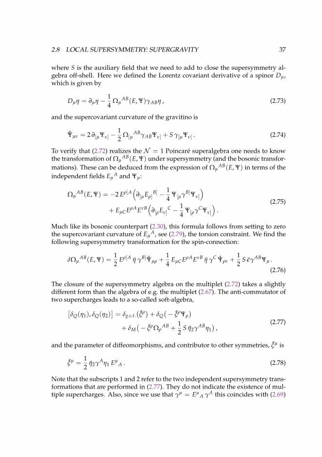
2.8 LOCAL SUPERSYMMETRY: SUPERGRAVITY 37
where S is the auxiliary field that we need to add to close the supersymmetry al-gebra off-shell. Here we defined the Lorentz covariant derivative of a spinor Dµ,which is given by
Dµη = ∂µη − 14
ΩµAB(E, Ψ)γABη , (2.73)
and the supercovariant curvature of the gravitino is
Ψµν = 2 ∂[µΨν] −12
Ω[µABγABΨν] + S γ[µΨν] . (2.74)
To verify that (2.72) realizes the N = 1 Poincare superalgebra one needs to knowthe transformation of Ωµ
AB(E, Ψ) under supersymmetry (and the bosonic transfor-mations). These can be deduced from the expression of Ωµ
AB(E, Ψ) in terms of theindependent fields Eµ
A and Ψµ:
ΩµAB(E, Ψ) = −2 Eρ[A
(∂[µEρ]
B] − 14
Ψ[µγB]Ψν]
)+ EµCEρAEνB
(∂[ρEν]
C − 14
Ψ[ργCΨν]
).
(2.75)
Much like its bosonic counterpart (2.30), this formula follows from setting to zerothe supercovariant curvature of Eµ
A, see (2.79), the torsion constraint. We find thefollowing supersymmetry transformation for the spin-connection:
δΩµAB(E, Ψ) =
12
Eρ[A η γB]Ψµρ +14
EµCEρAEνB η γC Ψρν +12
S εγABΨµ .
(2.76)
The closure of the supersymmetry algebra on the multiplet (2.72) takes a slightlydifferent form than the algebra of e.g. the multiplet (2.67). The anti-commutator oftwo supercharges leads to a so-called soft-algebra,[
δQ(η1), δQ(η2)]= δg.c.t.
(ξρ)+ δQ
(− ξρΨρ
)+ δM
(− ξρΩρ
AB +12
S η2γABη1)
,(2.77)
and the parameter of diffeomorphisms, and contributor to other symmetries, ξµ is
ξµ =12
η2γAη1 EµA . (2.78)
Note that the subscripts 1 and 2 refer to the two independent supersymmetry trans-formations that are performed in (2.77). They do not indicate the existence of mul-tiple supercharges. Also, since we use that γµ = Eµ
A γA this coincides with (2.69)

38 CHAPTER 2 BACKGROUND MATERIAL
when we take the rigid limit. The appearance of this soft-algebra stems from thefact that we introduced diffeomorphisms instead of local translations using (2.28).This is responsible for all the terms of the form ξµ times a gauge-field.
Of course all the curvatures shown in section 2.4 receive fermionic correctionsto account for the additional supersymmetry transformations of the gauge-fields.For example, we find
RµνA(E) = 2 ∂[µEν]
A − 2 Ω[µA
B Eν]B − 1
2Ψ[µγAΨν] . (2.79)
Supercovariant quantities such as (2.74) and (2.79) will be denoted with a hat todistinguish them from their bosonic counterparts.
In chapter 3, in fact in this whole thesis, we will focus mostly on extended su-pergravities with four supercharges, orN = 2 supersymmetry. A more detailed ar-gument againstN = 1 theories will be given in section 3.3. In short, non-relativisticsuperalgebras with only two supercharges do not lead to diffeomorphisms.
For later reference, we need on- and off-shell formulations of N = 2 Poincaresupergravity. We give the on-shell one here and we shall defer the presentation ofthe off-shell multiplet to the next chapter.
In general, superalgebras with more than one supercharge allow for central ex-tensions in the anti-commutator of two such charges. We will also include such acentral element, denoted by Z . Then, the N = 2 Poincare superalgebra is given by(2.15) and (2.66). Here we will focus on the on-shell version, where the gauge-fieldthat is related to the central charge transformation is not needed to close the alge-bra. Nevertheless, we will have to add it to take the non-relativistic limit, as we willshow in chapter 3, see section 3.4.
The on-shell N = 2 supergravity multiplet is given by
δEµA =
12
δij ηi γAΨµj , (2.80)
δΨµi = Dµηi = ∂µηi −14
ΩµABγABηi . (2.81)
The supersymmetry transformation of the dependent spin-connection,
δΩµAB(E, Ψi) = −
12
δij Eρ[A ηi γB]Ψµρj +14
δij EµCEρAEνB ηi γC Ψρνj , (2.82)
is zero on-shell, i.e. when we use the fermionic equation of motion
Ψµνi = 0 . (2.83)

2.8 LOCAL SUPERSYMMETRY: SUPERGRAVITY 39
The variation of ΩµAB(E, Ψi) follows from
ΩµAB(E, Ψ) = −2 Eρ[A
(∂[µEρ]
B] − 12
δij Ψ[µiγB]Ψν]j
)+ EµCEρAEνB
(∂[ρEν]
C − 14
δij Ψ[ρiγCΨν]j
),
(2.84)
which in turn is the solution to the supercovariant torsion constraint
RµνA(E) = 2 ∂[µEν]
A − 2 Ω[µA
B Eν]B − δij Ψ[µiγ
AΨν]j . (2.85)
This finishes our quick review of N = 2 on-shell Poincare supergravity.We note that in essence the only difference between theN = 1 andN = 2 theo-
ries is that all of the spinor variables take extra indices. This is somewhat special tothree dimensions though, because all supergravity fields are pure gauge and do notconstitute physical degrees of freedom. Thus, by adding more gravitini we do notadd fermionic degrees of freedom and the counting between bosonic and fermionicdegrees of freedom is not upset. In higher dimensions, adding more superchargesusually enforces also the addition of extra physical and auxiliary fields.

40
3A non-relativistic limiting procedure
This chapter contains the first main part of the thesis. Its aim is to introduce aprocedure that can be used to derive non-relativistic supergravity theories. Westart by stating the main ideas that underly this limiting procedure. Since thisis quite abstract we go on to discuss several examples. As a test we re-deriveNewton–Cartan gravity in arbitrary dimensions and on-shell Newton–Cartansupergravity in three space-time dimensions. We end by deriving a novel off-shell version of Newton–Cartan supergravity and, by extension of those results,an on-shell version of Newton–Hooke supergravity.
42 CHAPTER 3 A NON-RELATIVISTIC LIMITING PROCEDURE
This chapter begins the main part of this thesis. As laid out in the introduction, wewant to construct non-relativistic theories of supergravity. This chapter serves todescribe one way of doing so, based on our work in [110]. It is mainly organizedalong the same lines as that paper including one additional section on “less thanminimal” N = 1 Newton–Cartan supergravity.
In the following we develop a non-relativistic limiting procedure that enablesus to derive non-relativistic geometries and generally covariant (super)gravity the-ories from relativistic ones. In section 3.1 we explain the procedure itself in a ratherabstract way. To emphasize possible pitfalls, we use the procedure to re-deriveknown examples, i.e. theories that featured in the literature already. We beginby deriving with Newton–Cartan gravity in the formulation of [80] in section 3.2.Then, before moving on to “normal” N = 2 supergravity theories, we review thearguments for why we are mostly interested in theories with extended supersym-metry in section 3.3. We simply apply the limiting procedure on theN = 1 Poincaresupergravity theory which, for obvious reasons, does not lead to our preferredchoice of a non-relativistic theory of supergravity. In section 3.4 we re-derive theknown on-shell version of three-dimensional Newton–Cartan supergravity of [77]and in section 3.5 we obtain a new off-shell formulation of that theory. The lim-iting procedure is then applied to the relativistic point-particle with the aim of re-deriving the results of [111] in section 3.6. A short conclusion is presented in section3.7.
3.1 The general procedureIn this section we will describe the limiting procedure that we adopt in this chapterin general terms. This procedure can be viewed as an extension of the contractionof a relativistic space-time symmetry algebra to a non-relativistic one. Such con-tractions are known as so-called Inonu–Wigner contractions [96]. In particular, wetry to implement a similar contraction on an irreducible multiplet of fields, thatforms a representation of the relativistic algebra, to obtain an irreducible multipletof fields that represents the contracted non-relativistic algebra.
Recall that when performing a standard Inonu–Wigner contraction of a sym-metry algebra, one first redefines the generators of the algebra by taking linearcombinations of the original generators with coefficients that involve a contractionparameter ω. The contracted algebra is then obtained by calculating commutatorsof the redefined generators, re-expressing the result in terms of the redefined gen-erators and taking ω → ∞ in the end. Note that this procedure does not changethe number of generators and that for finite ω the algebra of redefined generatorsis equivalent to the original one.
We now wish to extend this contraction to an irreducible multiplet of fields thatforms a representation of a relativistic algebra. Such a multiplet will in generalcontain a number of independent fields that can be associated to certain genera-tors of the algebra. For instance, the vielbein of general relativity can be viewed
3.1 THE GENERAL PROCEDURE 43
as a gauge-field of local translations [95]. The other generators of the algebra areassociated to gauge-fields, that are however not independent, but that in generaldepend on all other independent fields in the multiplet. This is the way in whichthe spin-connection of general relativity can be viewed as a gauge-field of localLorentz transformations. Finally, the multiplet can also contain independent fieldsthat can not be interpreted as gauge-fields of the underlying space-time symmetryalgebra. This is for instance the case when considering off-shell supergravity mul-tiplets, where typically auxiliary fields are necessary to ensure that the number ofbosonic and fermionic degrees of freedom match.
In a first step, one can extend the algebra contraction to all fields in the multi-plet. This can be done first by extending the contraction from the generators to theparameters of symmetry transformations and to the gauge-fields that are associatedto the generators. Let us denote the original algebra generators collectively by TA,the original symmetry parameters by ξA and the original fields, that are associatedto the generators by AA
µ . The redefinition of the generators TA to generators TA,that involves ω and defines the contraction, can then be extended to redefinitionsof ξA to ξA and of AA
µ to AAµ such that
ξATA = ξATA , AAµ TA ' AA
µ TA . (3.1)
Strictly speaking, as we will clarify later in the specific examples, the second equa-tion only holds up to terms that are subleading in ω. For that reason we do not putan equality sign there.
The equation (3.1) defines the tilded parameters and fields in terms of the orig-inal ones and the contraction parameter ω. These definitions also guarantee that,for finite ω, the redefined multiplet is equivalent to the original one.
The defining equation (3.1) involves independent and dependent fields that areassociated to algebra generators. As far as the independent fields are concerned,this is the end of the story. Regarding the dependent fields, one should take intoaccount that the redefinition obtained from (3.1) should be consistent with the oneinduced by performing the redefinitions on the independent fields in the expres-sions that define dependent fields in terms of independent ones. This amounts toa non-trivial consistency check, as we will explain in the next paragraph. By ex-amining the transformation rules in terms of redefined parameters and fields, onecan then define redefinitions of the fields that are not associated to gauge trans-formations, by requiring that no term in the transformation rules diverges whentaking the limit ω → ∞. As we will see later in a specific example, this step usuallyamounts to rescaling these fields with the contraction parameter ω.
After having determined the necessary redefinitions of all fields, one can sendω → ∞, at which point the consistency of the procedure needs to be checked. Ina first step, checking consistency involves ensuring that no divergences appear inthe procedure. This means for instance that one needs to examine whether thetransformation rules in terms of redefined quantities are finite in the limit ω → ∞.Moreover, one needs to examine the expressions of the dependent fields in terms of
44 CHAPTER 3 A NON-RELATIVISTIC LIMITING PROCEDURE
the independent ones and check whether one obtains a finite result, consistent withthe redefinition implied by (3.1), when writing these expressions in terms of rede-fined independent fields and taking ω → ∞. As we will see in specific examples,this step involves imposing additional constraints on the fields.
Typically, these constraints involve putting certain covariant quantities to zero.These covariant quantities might for instance correspond to gauge covariant curva-tures of fields that are interpreted as gauge-fields of the algebra. Constraining thefields in such a covariant way will ensure that the final transformation rules are theproper ones.
Once a set of constraints is obtained by requiring that transformation rules andother quantities do not diverge when ω → ∞, one needs to check whether theseconstraints form a consistent set. This involves varying all non-trivial constraintsfound so far under all symmetry transformations and checking that they form aclosed set. In this way, one ensures that one is performing a consistent truncation.
Finally, we mention that the limiting procedure can lead to the elimination of anumber of auxiliary fields. This is due to the fact that we are interested in obtainingan irreducible multiplet. The non-relativistic theory can have less equations of mo-tion than the relativistic one hence the number of auxiliary fields that are neededto realize the non-relativistic algebra can differ from the number that is needed torealize the relativistic algebra. This is responsible for the fact that some auxiliaryfields have to be eliminated in the limiting process.
We can summarize the procedure in the following way:
I. We first write the relativistic gauge-fields in terms of new ‘non-relativistic’ones, using a contraction parameter ω. For finite ω this is a field redefinitionthat is dictated by the contraction of the generators of the algebra. At thispoint the scaling of the auxiliary fields is still arbitrary.
II. Using the above redefinitions and taking the limit ω → ∞ we can derive a firstset of non-relativistic constraints by taking the limit ω → ∞ of the relativisticun-conventional constraints.
III. In a next step, we derive the transformation rules of all fields. Requiringthat no terms diverge in the limit ω → ∞ fixes the scalings of the auxiliaryfields. At this point, we can check the limit of dependent gauge-fields, suchas e.g. the spin-connection. Requiring that they have a well-defined limit caninvolve the use of un-conventional constraints, written in terms of redefinedfields, to replace divergent terms by terms with a proper limit.
IV. In this step, we check whether the constraints found in step two are a closedset under the different symmetry transformations or whether we are forced tointroduce additional constraints. An example were many new constraints arefound by continuous variation under supersymmetry is given by the chain ofconstraints in eqs. (3.65)–(3.67).
V. The number of auxiliary fields that are needed in the non-relativistic case canbe less then the number that is needed in the relativistic case. In such cases, inorder to obtain an irreducible multiplet, we eliminate the redundant auxiliary

3.2 NEWTON–CARTAN GRAVITY 45
fields. This occurs, for instance, in the example of section 3.5.
In the next sections, we will illustrate this procedure by using it to re-derivevarious results on Newton–Cartan geometry and (super)gravity that have been ob-tained by other methods.
3.2 Newton–Cartan gravityIn the following, we illustrate the limiting procedure in one of its simplest manifes-tations, by deriving the Newton–Cartan theory of gravity of [80] from the vielbeinformulation of general relativity. The starting point was conveniently summarizedin the last chapter in section 2.4 where we discussed general relativity from pre-cisely the point of view that we need here. We will pay attention to how we derivethe transformation rules of the non-relativistic gauge-fields and how we derive con-straints that those background fields have to obey.
As should be clear from the general discussion in the last section, the limit-ing procedure is based on the Inonu–Wigner contraction of symmetry algebras. Inparticular, now we need to look at the non-relativistic contraction of the Poincarealgebra that yields the Bargmann algebra [96,98]. To obtain the Galilei algebra witha central extension we need to add an extra generator to the Poincare algebra. Thenumber of generators stays the same in the contraction and the Poincare and Galileialgebras already have the same number of generators. Hence, to get an extra gen-erator we need to add it already to the Poincare algebra. In the bosonic case, theonly way to do so is to trivially extend the Poincare algebra with an extra U(1)symmetry that is generated by the new operator Z . The contraction then consistsof rescaling the generators of the Poincare algebra and Z in the following way:
P0 →1
2ωH + ω Z , Z → 1
2ωH −ω Z , Ma0 → ω Ga . (3.2)
The spatial translations Pa and rotations, which we will denote by Mab = Jab, arenot rescaled. Calculating the commutators of H, Pa, Ga, Jab and Z, re-expressingeverything in terms of the relativistic generators and taking ω → ∞ leads to thenon-vanishing commutators of the Bargmann algebra given in (2.45) and (2.46).
In [80] Newton–Cartan gravity was obtained by gauging the Bargmann alge-bra. Our aim is to derive the same formulation of Newton–Cartan gravity via acontraction of the relativistic background fields Eµ
A and ΩµAB(E) that follow from
gauging the Poincare algebra as we explained in chapter 2.Let us mention at this point that the contraction (3.2) is not unique. Rather, it
corresponds a particular non-relativistic “point-particle limit” where time is singledout as a special direction. One can define more general p-brane limits where onetime and p spatial directions are singled out, see e.g. [62,63,65,101]. For the purposeof this thesis we will only concentrate on the “particle limit”.
In this first instance of the limiting procedure we shall be very careful about
46 CHAPTER 3 A NON-RELATIVISTIC LIMITING PROCEDURE
which quantities are non-relativistic ones, i.e. which are obtained in the limit ω →∞, and which ones are merely redefined relativistic ones, i.e. with finite contractionparameter ω. We will denote the latter ones with tildes and drop those tildes as welet ω → ∞.
The main idea of the limiting procedure is to extend the contraction (3.2) to thegauge-fields. Hence, we will take the first two formulas in (3.2) as a motivation forthe expansion of our relativistic background fields in terms of the Newton–Cartanones. The result is the following ansatz for the relativistic vielbein:
EµA = δA
0
(ω τµ +
12ω
mµ
)+ δA
a eµa . (3.3)
Ultimately, τµ, eµa and mµ will become the background fields of Newton–Cartan
gravity. Then we shall also use projective inverses of τµ and eµa, which we denote
by τµ and eµa, that are defined as follows:
eµa eµ
b = δba , τµτµ = 1 , τµ eµ
a = 0 ,
τµ eµa = 0 , eρ
a eµa = δ
ρµ − τµτρ .
(3.4)
From here we can immediately deduce the following expansion of the relativisticinverse vielbein in terms of the non-relativistic components:
EµA = δa
A
[eµ
a +O( 1
ω2
)]+
1ω
δ0A
[τµ +O
( 1ω2
)]. (3.5)
Note that we have only explicitely given the terms of leading order in ω. There arein principle an infinite number of corrections which, however, will not be neededin the following as they do not contribute in the limit ω → ∞.
Extending the contraction (3.2) to the gauge-field Mµ that is related to the U(1)generator Z , we find the expansion
Mµ = ω τµ −1
2ωmµ . (3.6)
Since this gauge-field did not take part in the discussion on the kinematics of gen-eral relativity in chapter 2 we shall collect some more important formulas concern-ing it here. The transformation rule of Mµ is given by
δMµ = ξρ∂ρ Mµ + Mρ∂µξρ + ∂µΛ , (3.7)
where Λ is the parameter of the spurious U(1) symmetry. The covariant curvatureof Mµ reads
Fµν(M) = 2 ∂[µ Mν] . (3.8)
In the following we will need to impose constraints on this curvature. In the
3.2 NEWTON–CARTAN GRAVITY 47
bosonic case that we discuss in this section we have two options:
dynamical : Fµν(M) = 0 , (3.9)
kinematical : eµa eν
b Fµν(M) = Fab(M) = 0 . (3.10)
If we are interested in the dynamical theory, we set the full curvature Fµν(M) tozero. Then Mµ is a pure gauge-field and does not propagate, so we do not addany degrees of freedom to general relativity. However, we will see that, in orderto take the non-relativistic limit in a consistent manner, we need not impose sucha strict constraint. It turns out that if we are only interested in deriving the correctkinematics, it is sufficient to require that only the spatial projection of the curvaturevanishes, i.e. we can opt for the “kinematical” constraint (3.10).
In principle we can extend the contraction (3.2) to find the rescaling of the de-pendent gauge-fields. Their dependence on other independent gauge-fields is aconsequence of constraints. We might consider taking the non-relativistic limit ofthose un-conventional constraints too. However, this should not lead to any newinformation, provided we are able to take the limit in the expression for the depen-dent gauge-fields in a consistent way. Having used the relativistic torsion constraintto solve for the relativistic spin-connection, we cannot obtain new information bytaking its limit. It still remains an identity that we use to solve for Ωµ
AB(E).It turns out that in order to take the limit of the explicit expression (2.30) we need
an extra constraint to replace a term that diverges in the limit ω → ∞ by a finiteone. To this end, we have to make use of the extra gauge-field Mµ and impose oneof the two constraints (3.9) and (3.10) on its curvature (3.8). Now we can define thenon-relativistic spin- and boost-connection by
Ωµab(E) +
ω
2τµ eρa eνb Fρν(M) = ωµ
ab(e, τ, m) +O( 1
ω2
), (3.11)
Ωµ0a(E)− 1
2eµ
b eρb eνa Fρν(M) =1ω
ωµa(e, τ, m) +O
( 1ω3
). (3.12)
When inserting the redefinitions (3.3) and (3.6) in (2.30) we find
ωµab(e, τ, m) = −2 eν[a∂[µ eν]
b] + eµc eρa eνb∂[ρ eν]
c − τµ eρa eνb∂[ρmν] , (3.13)
ωµa(e, τ, m) = τν∂[µ eν]
a + eµb eρaτν∂[ρ eν]
b + eνa∂[µmν] − τµ eρaτν∂[ρmν] . (3.14)
A few comments are in order. First, the subleading contributions in the definitions(3.11) and (3.12) are due to the subleading terms in the expansion of the relativisticinverse vielbein (3.5). Secondly, note that while the constraint Fµν(M) is trivial inthe relativistic case, by adding it to the spin-connection we are effectively splittingit up into different parts. The leading part will cancel the leading (divergent) con-tribution of Ωµ
AB(E), while the subleading part remains as a finite contribution tothe non-relativistic connections. Hence, we need to be very careful and check if thedefinitions (3.11) and (3.12) are indeed consistent when we take the limit ω → ∞.
48 CHAPTER 3 A NON-RELATIVISTIC LIMITING PROCEDURE
Moreover, we have to ensure that the constraints (3.9) and (3.10) remain valid in thelimit, i.e. we shall investigate their limits too.
Note that the scaling of all gauge-fields (3.3), (3.6), (3.11) and (3.12) are suchthat the sum of the products of the gauge-fields with their respective symmetrygenerator remains invariant, up to subleading terms in ω. One thus has
PA EµA +Z Mµ + MAB Ωµ
AB(E) =
Pa eµa + H τµ + Z mµ + Jab ωµ
ab(e, τ, m)− 2 Ga ωµa(e, τ, m) +O
( 1ω2
).
(3.15)
The factor −2 in the last term is due to our definition of ωµa(e, τ, m), see (3.12).
Note also the appearance of the subleading terms in ω that we referred to after(3.1). They are also due to the definitions (3.11) and (3.12).
Now we proceed to take the limit ω → ∞ and drop the tildes on all fields.We start by calculating the transformation rules of the Newton–Cartan backgroundfields τµ, eµ
a and mµ, by applying (3.3) and (3.6) to (2.20). To do so, we express thenew fields in terms of the old ones, i.e.
τµ =1
2ω
(Eµ
0 + Mµ
), mµ = ω
(Eµ
0 −Mµ
). (3.16)
Then it is straightforward to get
δτµ = 0 ,
δeµa = λa
b eµb + λaτµ ,
δmµ = ∂µσ + λa eµa ,
(3.17)
where we defined
λa = ω λa0 , Λ = − σ
ω. (3.18)
All fields transform also under diffeomorphisms in the usual way. The transforma-tions of the spin-connections can be found as well:
δωµab(e, τ, m) = ∂µλab + 2 λ[a
c ωµcb] , (3.19)
δωµa(e, τ, m) = ∂µλa + λa
b ωµb −ωµ
ac λc . (3.20)
The transformation rules (3.17)–(3.20) agree with those found in [80] by gaugingthe Bargmann algebra.
Next, we take a look at the constraints of the non-relativistic theory. The expres-sions (3.13) and (3.14) (without the tildes) agree with those of [80]. In their analysis
3.2 NEWTON–CARTAN GRAVITY 49
these expressions were obtained by solving the constraints
Rµνa(P) = 2 ∂[µeν]
a − 2 ω[µabeν]
b − 2 ω[µaτν] = 0 ,
Rµν(Z) = 2 ∂[µmν] − 2 ω[µaeν]
a = 0 .(3.21)
Hence, these are also satisfied in our case. Next, we look at the implications of (3.9)and (3.10). Here, we have two possibilities. The “dynamical” constraint (3.9) leadsto
Rµν(H) = 2 ∂[µτν] = 0 , (3.22)
a constraint that was also used in [80]. The other option is to set only the spatialprojection to zero, i.e.
Rab(H) = 2 eµaeν
b ∂[µτν] = 0 . (3.23)
Note that this could be solved by
2 ∂[µτν] = b[µτν] , (3.24)
where bµ is arbitrary. This equation resembles the curvature constraint of the twist-less torsional Newton–Cartan theory [29]. In both cases, (3.22) or (3.23), the vari-ation of this constraint does not lead to any further restriction as τµ is invariantunder gauge transformations.
Further constraints stem from the relativistic Bianchi identity. Using the inversevielbein (3.5) and the expansion
RµνAB(Ω) = δA
a δBb Rµν
ab( J)− 1ω
δAa δB
0 Rµνa(G) +
1ω
δA0 δB
b Rµνb(G) , (3.25)
in (2.34) we obtain the non-relativistic Bianchi identities
R[µνa(G) eρ]
a = 0 , R[µνab(J) eρ]
a + R[µνb(G) τρ] = 0 , (3.26)
for the following curvatures of spatial rotations and Galilean boosts:
Rµνab(J) = 2 ∂[µων]
ab − 2 ω[µa
cων]cb ,
Rµνa(G) = 2 ∂[µων]
a − 2 ω[µabων]
b .(3.27)
This concludes the search for constraints of the kinematical theory. As we are in-terested primarily in the kinematics we did not derive equations of motion yet. Wemay impose equations of motion on the Newton–Cartan background fields, for ex-ample by taking the non-relativistic limit of the Einstein equation. This will lead to
50 CHAPTER 3 A NON-RELATIVISTIC LIMITING PROCEDURE
the exact theory presented in [80]. The limit yields the equations
Rµνab(J) eµ
a = 0 , Rµνa(G) eµ
a = 0 . (3.28)
If we choose to solve the first equation by setting Rµνab(J) = 0, which will be
needed in the supersymmetric on-shell case, it follows from the Bianchi identitiesthat the only real equation of motion left is
R0aa(G) = 0 , (3.29)
all other (components of) curvatures being zero due to conventional constraints(3.21), one of the foliation constraints (3.22) or (3.23), or the choice Rµν
ab(J) = 0.The equation (3.29), when considering observers in a Galilean frame with only
time-dependent acceleration, reduces to the Poisson equation for the Newton po-tential, see [77,80]. In general, the right-hand-side is non-zero, but here it is becausewe took the limit of the Einstein equation without a source term. However, as wementioned in the introduction, in the special case of three space-time dimensions,we cannot write down a relativistic source term that would give rise to non-trivialsources after taking the non-relativistic limit. Therefore, in three dimensions thelimit of the Einstein equation will always be (3.29) unless we add a source by hand.Hence, there is no non-trivial, normalizable solution for the Newton potential inthree dimensions. In this sense, we do not find any contradiction with the factthere should be no force between point-particles in “ordinary” three-dimensionalnon-relativistic gravity.
Finally, let us try to understand, from the point of this limiting procedure, whythere is no action for Newton–Cartan gravity. What happens if we simply takethe limit of the Einstein–Hilbert action (2.43)? The determinant of the relativisticvielbein will scale with one power of ω and the Ricci scalar expands to
R(Ω) = Rabab(J)− 2
ω2 R0aa(G) +O
( 1ω3
). (3.30)
Obviously the equations of motion (3.28) set this to zero. On the other hand, itis not obvious how an action consisting of only the leading term Rab
ab(J) wouldlead to both equations of (3.28). Moreover, due to the extra factor of ω from thedeterminant this term would diverge.
Previously we dealt with such divergences by imposing curvature constraints.However, none of those constraints was a limitation on Rµν
ab(J). It seems quiteunnatural to impose yet another, additional, constraint just to be able to get a finiteaction. An action that does not even lead to the correct equations of motion. Whilethis is not tight enough to serve as a no-go argument, it certainly is yet anotherindication that there is no action for Newton–Cartan gravity, at least not at the two-derivative level. Actions which consist of higher-derivative invariants have beenproposed in [20,103]. However, those papers do not derive the equations of motionthat constrain the background fields. Therefore, their connection to the theory of
3.3 NON-RELATIVISTIC N = 1 SUPERGRAVITY 51
Newton–Cartan gravity as we discussed it here is not completely clear to us.This concludes our first check of the non-relativistic limiting procedure. In the
following, we are going to investigate the limits of several supergravity theories.Therefore, from now on we shall restrict ourselves to theories in three space-timedimensions. We give a short exposition of non-relativistic N = 1 “supergravity”next, before we (re-)derive the on- and off-shell formulations of three-dimensionalNewton–Cartan supergravity theory.
3.3 Non-relativistic N = 1 supergravityThe discussion here and in the following sections parallels the one of the previoussection. We will therefore skip most intermediate steps, where the contraction pa-rameter ω is finite, and we will only focus on the results obtained in the ω → ∞limit. Here and in the following, we will therefore no longer resort to the notationusing tildes, to denote quantities at finite ω.
In this section we briefly review the argument of why we consider non-relativi-stic N = 2 supergravities as the minimal case, in place of the technically simplerN = 1 versions. To this end, we look at the non-relativistic contraction of theN = 1 Poincare superalgebra, (2.15) and (2.65). Again, we add an extra U(1) toget the central charge of the Bargmann superalgebra. The scaling of the bosonicgenerators is given in (3.2) and the fermionic supercharge Q must scale as
Q =√
ω Q− . (3.31)
In addition to the bosonic commutation relations of the Bargmann algebra we get
[Jab, Q−
]= −1
2γabQ− ,
Q−, Q−
= γ0C−1 Z . (3.32)
Notice that the anti-commutator of two supercharges leads to a central charge trans-formation but no time- or space-translation. Normally, the anti-commutator of twosupercharges leads to a diffeomorphism, see e.g. (2.65) or (2.66). So while theN = 1extended Bargmann algebra is perfectly well-defined, we rather not call it a superal-gebra in the usual sense, simply because the anti-commutator of two superchargesdoes not lead to diffeomorphisms.
We can demonstrate this too by looking at the explicit transformation rules ofthe background fields τµ, eµ
a, mµ and ψµ−, which we derive from (2.72) using thelimiting procedure. This shall also serve as a first easy example of the limitingprocedure in the supersymmetric case. It also comprises a new result that has notbeen derived in the literature before, unlike the twoN = 2 formulations that followin section 3.4 and 3.5.
We must now specify the transformation of Mµ under supersymmetry. We use
δMµ = 0 , (3.33)
52 CHAPTER 3 A NON-RELATIVISTIC LIMITING PROCEDURE
and in order not to upset the counting of degrees of freedom we set the curvatureof Mµ to zero
Fµν(M) = 2 ∂[µ Mν] = 0 . (3.34)
This coincides of course with the bosonic constraint on Mµ that we imposed in thelast section 3.2, see eq. (3.8). Then Mµ is pure gauge and does not propagate anydegrees of freedom. Otherwise we would, due to the addition of the extra field Mµ,have more bosonic degrees of freedom than fermionic ones in the multiplet (2.72).
Furthermore, the transformation rule (3.33) makes sure that the constraint (3.34)does not lead to any additional conditions on the gauge-fields as its supersymmetrytransformation does not lead to more constraints. Also, the supersymmetry algebra(2.77) is realized on Mµ through (3.34):[
δ1, δ2]Mµ = 0 = ξρ∂ρ Mµ + Mρ∂µ ξρ − ∂µ
(ξρ Mρ
)= ξρ Fρµ(M) . (3.35)
The last term in the soft-algebra on Mµ is not present in (2.77) because we didnot consider the additional U(1) generator then. It should be clear, by comparingvarious soft-algebras in this work, that we naturally expect it to take this form.
This concludes our discussion of the relativistic starting point. Next, we willtake the non-relativistic limit to derive transformation rules and constraints. First,we need to define how to scale the spinors. Following our general rules on how totake the limit we use the contraction (3.3) and (3.6), plus the new rule
Ψµ =1√ω
ψµ− , (3.36)
which follows promptly from the formula (3.31). Furthermore, we need to use
S→ 1ω
S , (3.37)
when taking the limit of the off-shell multiplet (2.72). Then, we find the transfor-mation rules of the non-relativistic N = 1 off-shell multiplet
δτµ = 0 ,
δeµa = 0 ,
δmµ =12
ε−γ0ψµ− ,
δψµ− = Dµε− +12
S τµ γ0ε− ,
δS =18
ε−γabψab− .
(3.38)
The transformation rules of the dependent spin-connections, which are obtained
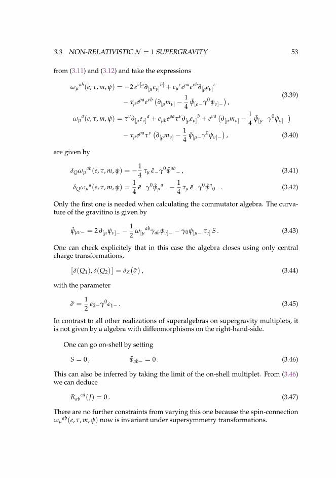
3.3 NON-RELATIVISTIC N = 1 SUPERGRAVITY 53
from (3.11) and (3.12) and take the expressions
ωµab(e, τ, m, ψ) = −2 eν[a∂[µeν]
b] + eµceρaeνb∂[ρeν]
c
− τµeρaeνb (∂[ρmν] −14
ψ[ρ−γ0ψν]−)
,(3.39)
ωµa(e, τ, m, ψ) = τν∂[µeν]
a + eµbeρaτν∂[ρeν]b + eνa (∂[µmν] −
14
ψ[µ−γ0ψν]−)
− τµeρaτν(∂[ρmν] −
14
ψ[ρ−γ0ψν]−)
, (3.40)
are given by
δQωµab(e, τ, m, ψ) = −1
4τµ ε−γ0ψab
− , (3.41)
δQωµa(e, τ, m, ψ) =
14
ε−γ0ψµa− −
14
τµ ε−γ0ψa0− . (3.42)
Only the first one is needed when calculating the commutator algebra. The curva-ture of the gravitino is given by
ψµν− = 2 ∂[µψν]− −12
ω[µabγabψν]− − γ0ψ[µ− τν] S . (3.43)
One can check explicitely that in this case the algebra closes using only centralcharge transformations,[
δ(Q1), δ(Q2)]= δZ
(σ)
, (3.44)
with the parameter
σ =12
ε2−γ0ε1− . (3.45)
In contrast to all other realizations of superalgebras on supergravity multiplets, itis not given by a algebra with diffeomorphisms on the right-hand-side.
One can go on-shell by setting
S = 0 , ψab− = 0 . (3.46)
This can also be inferred by taking the limit of the on-shell multiplet. From (3.46)we can deduce
Rabcd(J) = 0 . (3.47)
There are no further constraints from varying this one because the spin-connectionωµ
ab(e, τ, m, ψ) now is invariant under supersymmetry transformations.
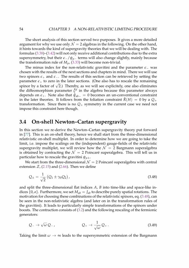
54 CHAPTER 3 A NON-RELATIVISTIC LIMITING PROCEDURE
The short analysis of this section served two purposes. It gives a more detailedargument for why we use onlyN = 2 algebras in the following. On the other hand,it hints towards the kind of supergravity theories that we will be dealing with. Theformulas (3.38)–(3.42) will not only receive additional contributions due to the extrasupersymmetry, but their ε−/ψµ− terms will also change slightly, mainly becausethe transformation rule of Mµ, (3.33) will become non-trivial.
The minus index for the non-relativistic gravitini and the parameter ε− waschosen with the results of the next sections and chapters in mind. There we will usetwo spinors ε+ and ε−. The results of this section can be retrieved by setting theparameter ε+ to zero in the later sections. (One also has to rescale the remainingspinor by a factor of
√2.) Thereby, as we will see explicitely, one also eliminates
the diffeomorphism parameter ξµ in the algebra because this parameter alwaysdepends on ε+. Note also that ψab− = 0 becomes an un-conventional constraintin the later theories. It follows from the foliation constraint R(H) = 0 by a Q+
transformation. Since there is no Q+ symmetry in the current case we need notimpose this constraint here though.
3.4 On-shell Newton–Cartan supergravityIn this section we re-derive the Newton–Cartan supergravity theory put forwardin [77]. This is an on-shell theory, hence we shall start from the three-dimensionalrelativistic on-shell multiplet. In order to determine how we are going to take thelimit, i.e. impose the scalings on the (independent) gauge-fields of the relativisticsupergravity multiplet, we will review how the N = 2 Bargmann superalgebrais obtained by contracting the N = 2 Poincare superalgebra. This will tell us inparticular how to rescale the gravitini ψµ±.
We start from the three-dimensional N = 2 Poincare superalgebra with centralextension Z , (2.15) and (2.66). Then we define
Q± =1√2
(Q1 ± γ0Q2
), (3.48)
and split the three-dimensional flat indices A, B into time-like and space-like in-dices 0, a. Furthermore, we set Mab = Jab to describe purely spatial rotations. Themotivation for choosing these combinations of the relativistic spinors, eq. (3.48), canbe seen in the non-relativistic algebra (and later on in the transformation rules ofthe gravitini). It leads to particularly simple transformations of the spinors underboosts. The contraction consists of (3.2) and the following rescaling of the fermionicgenerators:
Q− →√
ω Q− , Q+ →1√ω
Q+ . (3.49)
Taking the limit ω → ∞ leads to the supersymmetric extension of the Bargmann
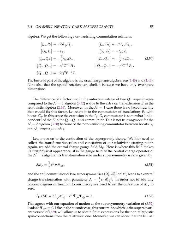
3.4 ON-SHELL NEWTON–CARTAN SUPERGRAVITY 55
algebra. We get the following non-vanishing commutation relations:[Jab, Pc
]= −2 δc[aPb] ,
[Jab, Gc
]= −2 δc[aGb] ,[
Ga, H]= −Pa ,
[Ga, Pb
]= −δab Z ,[
Jab, Q±]= −1
2γabQ± ,
[Ga, Q+
]= −1
2γa0Q− , (3.50)
Q+, Q+= −γ0C−1 H ,
Q+, Q−
= −γaC−1 Pa ,
Q−, Q−= −2 γ0C−1 Z .
The bosonic part of the algebra is the usual Bargmann algebra, see (2.45) and (2.46).Note also that the spatial rotations are abelian because we have only two spacedimensions.
The difference of a factor two in the anti-commutator of two Q− superchargescompared to the N = 1 algebra (3.32) is due to the extra central extension Z in therelativistic algebra (2.66). Moreover, in the N = 1 case there is no Jacobi identitythat would fix this factor, i.e. relate it to the commutator of translations Pa withboosts Ga. In this sense the extension in the Pa–Gb commutator is somewhat “inde-pendent” of the Z in the Q−–Q− anti-commutator. This is not true anymore for theN = 2 algebra (3.50) because of the non-vanishing commutator between boosts Gaand Q+ supersymmetry.
Lets move on to the contraction of the supergravity theory. We first need tocollect the transformation rules and constraints of our relativistic starting point.Again, we add the central charge gauge-field Mµ. Here is where this field makesits first physical appearance: it is the gauge field of the central charge operator ofthe N = 2 algebra. Its transformation rule under supersymmetry is now given by
δMµ =12
εij ηiΨµj , (3.51)
and the anti-commutator of two supersymmetries ([δ1i , δ2
j ]) on Mµ leads to a central
charge transformation with parameter Λ = 12 εij η1
i η2j . In order not to add any
bosonic degrees of freedom to our theory we need to set the curvature of Mµ tozero:
Fµν(M) = 2 ∂[µ Mν] − εij Ψ[µiΨν]j = 0 . (3.52)
This agrees with our equation of motion as the supersymmetry variation of (3.52)leads to Ψµνi = 0. Like in the bosonic case, this constraint, which is the supercovari-ant version of (3.9), will allow us to obtain finite expressions for the non-relativisticspin-connections from the relativistic one. Moreover, we can show that the full set
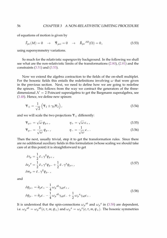
56 CHAPTER 3 A NON-RELATIVISTIC LIMITING PROCEDURE
of equations of motion is given by
Fµν(M) = 0 → Ψµνi = 0 → RµνAB(Ω) = 0 , (3.53)
using supersymmetry variations.
So much for the relativistic supergravity background. In the following we shallsee what are the non-relativistic limits of the transformations (2.80), (2.81) and theconstraints (3.51) and (3.53).
Now we extend the algebra contraction to the fields of the on-shell multiplet.For the bosonic fields this entails the redefinitions involving ω that were givenin the previous section. Next, we need to define how we are going to redefinethe spinors. This follows from the way we contract the generators of the three-dimensional N = 2 Poincare superalgebra to get the Bargmann superalgebra, see(3.48). Hence, we define new spinors
Ψ± =1√2
(Ψ1 ± γ0Ψ2
), (3.54)
and we will scale the two projections Ψ± differently:
Ψµ+ =√
ω ψµ+ , η+ =√
ω ε+ , (3.55)
Ψµ− =1√ω
ψµ− , η− =1√ω
ε− . (3.56)
Then the next, usually trivial, step it to get the transformation rules. Since thereare no additional auxiliary fields in this formulation (whose scaling we should takecare of at this point) it is straightforward to get
δτµ =12
ε+γ0ψµ+ ,
δeµa =
12
ε+γaψµ− +12
ε−γaψµ+ ,
δmµ = ε−γ0ψµ− ,
(3.57)
and
δψµ+ = ∂µε+ −14
ωµabγabε+ ,
δψµ− = ∂µε− −14
ωµabγabε− +
12
ωµaγa0ε+ .
(3.58)
It is understood that the spin-connections ωµab and ωµ
a in (3.58) are dependent,i.e. ωµ
ab = ωµab(e, τ, m, ψ±) and ωµ
a = ωµa(e, τ, m, ψ±). The bosonic symmetries

3.4 ON-SHELL NEWTON–CARTAN SUPERGRAVITY 57
act on the spinors in the following way:
δψµ+ =14
λabγabψµ+ ,
δψµ− =14
λabγabψµ− −12
λaγa0ψµ+ .(3.59)
This stems from the relativistic δΨµ = 14 λABγABΨµ.
The expressions for the spin-connections follow from (2.84) and (3.52). Like inthe bosonic case discussed in section 3.2, we use (3.52) to replace terms that divergein the limit ω → ∞, by terms with the expected ω-order. We get
ωµab = −2eν[a(∂[µeν]
b] − 12
ψ[µ+γb]ψν]−)+ eµ
ceρaeνb(∂[ρeν]c − 1
2ψ[ρ+γcψν]−
)− τµeρaeνb(∂[ρmν] −
12
ψ[ρ−γ0ψν]−)
, (3.60)
and
ωµa = τν
(∂[µeν]
a − 12
ψ[µ+γaψν]−)+ eµbeρaτν
(∂[ρeν]
b − 12
ψ[ρ+γbψν]−)
+ eνa(∂[µmν] −12
ψ[µ−γ0ψν]−)− τµeρaτν
(∂[ρmν] −
12
ψ[ρ−γ0ψν]−)
.
(3.61)
These expressions for the spin- and boost-connection also solve the supercovariantcurvature constraints
Rµνa(P) = Rµν
a(P)− ψ[µ+γaψν]− = 0 ,
Rµν(Z) = Rµν(Z)− ψ[µ−γ0ψν]− = 0 ,(3.62)
identically. To check the consistency of the set of constraints, i.e. to derive the im-plications of (3.52) we need the transformations of the spin-connections under su-persymmetry. The explicit expressions (3.60) and (3.61), or the constraints (3.62),can be used for that purpose. We find
δQωµab =
12
ε+γ[bψa]µ− +
14
eµc ε+γcψab− −
12
τµ ε−γ0ψab−
+12
ε−γ[bψa]µ+ +
14
eµc ε−γcψab+ ,
(3.63)
δQωµa =
12
ε−γ0ψµa− +
12
τµ ε−γ0ψ0a− +
14
eµb ε+γbψa0− +
14
ε+γaψµ0−
+14
eµb ε−γbψa0+ +
14
ε−γaψµ0+ . (3.64)
Now we readily derive that the following set of constraints is generated under su-
58 CHAPTER 3 A NON-RELATIVISTIC LIMITING PROCEDURE
persymmetry transformations:
Q−−→ ψab− = 0 (3.65)
Rµν(H) = 0Q+−→ ψµν+ = 0
Q+−→ Rµνab(J) = 0 (3.66)
Q+−→ γaψa0− = 0Q+−→ R0a
a(G) = 0 .(3.67)
Using the last equation of (3.66), the non-relativistic Bianchi identities reduce to
Rabc(G) = 0 , R0[a
b](G) = 0 , (3.68)
which ensures e.g. that (3.65) does not lead to further constraints. The superco-variant curvature of Galilean boosts, which is used in the formulas above, is givenby
Rµνa(G) = Rµν
a(G)− 2 ψ[µ−γ0ψν]a−
− 12
e[νb ψµ]+γbψa
0− −12
ψ[µ+γaψν]0− .(3.69)
The variation of the last constraint in (3.67) is quite involved and has also notbeen carried out in [77]. We will, however, show in section 3.5 that the full set ofconstraints (3.65)–(3.67) can be derived from an off-shell version of this multiplet.There it is easier to check the consistency of the whole set of constraints.
At this point we have finished the derivation of the three-dimensional on-shellNewton–Cartan supergravity constructed in [77], i.e. we obtained all constraintsand transformation rules. The terminology “on-shell” stems from the fact thatthe constraints given in eq. (3.67) both can be interpreted as equations of motionfor Newton–Cartan supergravity: the first constraint is necessary to obtain clo-sure of the supersymmetry algebra, while the bosonic part of the second constraintis precisely the equation of motion of the bosonic Newton–Cartan gravity theory.Note, however, that to call some constraints “equation of motion” and others not isslightly ambiguous when talking about Newton–Cartan (super)gravity, due to theabsence of an action principle that can be used to derive these equations of motion.In section 3.5, we will construct a different, “off-shell” version of three-dimensionalNewton–Cartan supergravity, that includes an auxiliary scalar field in the super-multiplet. The terminology “off-shell” will be justified in the sense that the firstconstraint given in eq. (3.67) will no longer be needed for closure of the supersym-metry algebra. Both constraints given in eq. (3.67) will in fact not appear at all.Equations of motion can thus be identified in a pragmatic way as those constraintsthat can be removed by adding auxiliary degrees of freedom to a non-relativisticsupermultiplet.
Let us stress/repeat some important aspects. In the case at hand, we can drawthe following diagram, see figure 3.1. It shows that we can always derive a non-
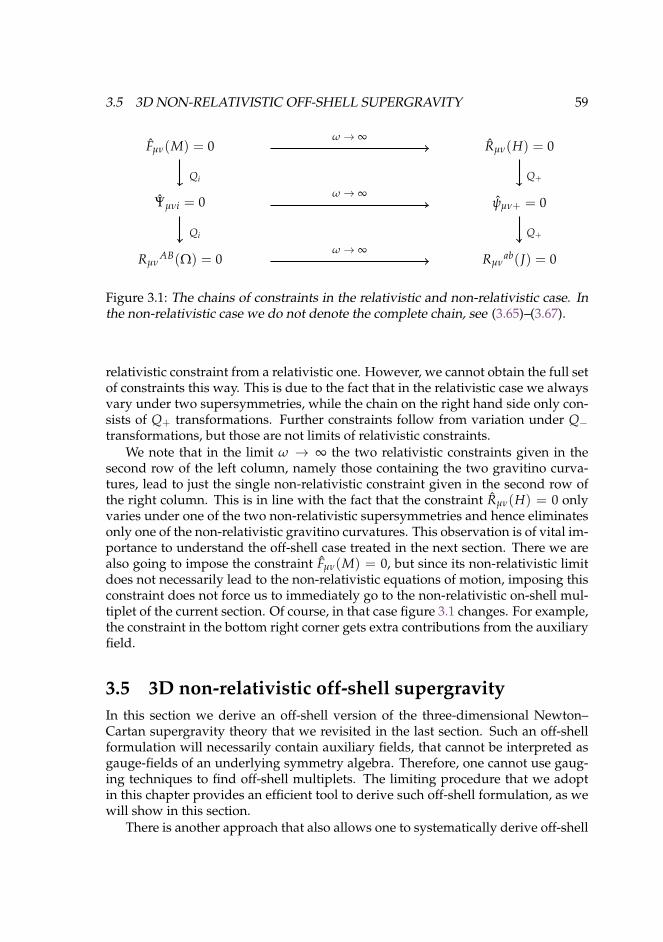
3.5 3D NON-RELATIVISTIC OFF-SHELL SUPERGRAVITY 59
Qi
Qi
Fµν(M) = 0
Ψµνi = 0
RµνAB(Ω) = 0
Q+
Q+
Rµν(H) = 0
ψµν+ = 0
Rµνab(J) = 0
ω → ∞
ω → ∞
ω → ∞
Figure 3.1: The chains of constraints in the relativistic and non-relativistic case. Inthe non-relativistic case we do not denote the complete chain, see (3.65)–(3.67).
relativistic constraint from a relativistic one. However, we cannot obtain the full setof constraints this way. This is due to the fact that in the relativistic case we alwaysvary under two supersymmetries, while the chain on the right hand side only con-sists of Q+ transformations. Further constraints follow from variation under Q−transformations, but those are not limits of relativistic constraints.
We note that in the limit ω → ∞ the two relativistic constraints given in thesecond row of the left column, namely those containing the two gravitino curva-tures, lead to just the single non-relativistic constraint given in the second row ofthe right column. This is in line with the fact that the constraint Rµν(H) = 0 onlyvaries under one of the two non-relativistic supersymmetries and hence eliminatesonly one of the non-relativistic gravitino curvatures. This observation is of vital im-portance to understand the off-shell case treated in the next section. There we arealso going to impose the constraint Fµν(M) = 0, but since its non-relativistic limitdoes not necessarily lead to the non-relativistic equations of motion, imposing thisconstraint does not force us to immediately go to the non-relativistic on-shell mul-tiplet of the current section. Of course, in that case figure 3.1 changes. For example,the constraint in the bottom right corner gets extra contributions from the auxiliaryfield.
3.5 3D non-relativistic off-shell supergravityIn this section we derive an off-shell version of the three-dimensional Newton–Cartan supergravity theory that we revisited in the last section. Such an off-shellformulation will necessarily contain auxiliary fields, that cannot be interpreted asgauge-fields of an underlying symmetry algebra. Therefore, one cannot use gaug-ing techniques to find off-shell multiplets. The limiting procedure that we adoptin this chapter provides an efficient tool to derive such off-shell formulation, as wewill show in this section.
There is another approach that also allows one to systematically derive off-shell
60 CHAPTER 3 A NON-RELATIVISTIC LIMITING PROCEDURE
formulations, the superconformal tensor calculus. This though is the theme ofchapter 6, were will derive two off-shell formulations, one of them being the newminimal Newton–Cartan supergravity theory that we also derive in this section.We proceed now with taking the limit.
We shall take the non-relativistic limit of a three-dimensional N = 2 off-shelltheory of supergravity. There exist two different off-shell formulations of N = 2supergravity in three dimensions [112–114]. To determine which one we shouldfocus on, we take a look at the fields and transformation rules that we used toderive the on-shell theory. We will use the so-called new minimal N = 2 Poincaremultiplet because this multiplet contains the abelian central charge gauge-field Mµ
that was already part of the on-shell analysis. It is not obvious to us how to take thenon-relativistic limit of the old minimal N = 2 Poincare multiplet due to the lackof this abelian gauge-field with the transformation rule given in (3.51). Therefore,we shall not try to do so here but we focus only on the new minimal formulation.
The new minimal N = 2 Poincare multiplet consists of the dreibein EµA, two
gravitini Ψµi (i = 1, 2), two vector gauge-fields Mµ and Vµ and an auxiliary scalarD, see e.g. [114]. The supersymmetries, central charge transformations and R-symmetry transformations, with parameters ηi, Λ and ρ respectively, are given by
δEµA =
12
δij ηi γA Ψµj ,
δΨµi = Dµηi − γµηi D + εij ηj Vµ +14
γµ γ · F(M) εij ηj − εij Ψµj ρ ,
δMµ =12
εij ηi Ψµj + ∂µΛ ,
δVµ =12
εij ηi γνΨµνj −18
εij ηi γµγ · Ψj −14
δij ηi γ · F(M)Ψµj
− εij ηi Ψµj D + ∂µρ ,
δD = − 116
δij ηi γ · Ψj .
(3.70)
The field strengths are given by (3.52) and
Ψµνi = 2 D[µΨν]i − 2 γ[µΨν]i D− 2 εij Ψ[µj Vν] +12
εij γ[µγ · F(M)Ψν]j , (3.71)
and dots refer to gamma traces as in γ · F(M) = γµν Fµν(M). The spin-connection isdetermined by requiring the torsion Rµν
A(E) be zero. Its supersymmetry variationfollows from the expression in terms of the independent fields Eµ
A and Ψµi.In order to take the non-relativistic limit of (3.70) we use the same rescalings as
in the previous sections, supplemented with the rule
D =1ω
S . (3.72)
3.5 3D NON-RELATIVISTIC OFF-SHELL SUPERGRAVITY 61
In the action of the N = 2 new minimal supergravity the D2 term plays the role ofthe cosmological constant ΛCC. It is thus not surprising that in the non-relativisticlimit, D scales like the square root of ΛCC. For the non-relativistic contraction ofthe anti-de Sitter algebra see e.g. [111]. We do not rescale the field Vµ. Moreover,below we will argue that in the non-relativistic limit one must to eliminate Vµ.1
Going through similar arguments as in sections 3.2 and 3.4 we determine thenon-relativistic dependent spin-connections ωµ
ab(e, τ, m, ψ±) and ωµa(e, τ, m, ψ±)
to be given by (3.60) and (3.61). They also satisfy (3.62). As in the on-shell casewe need to impose (3.52) as an extra constraint and we also need to eliminate thecurvature ψµν+ in order to take the limit in a consistent manner. Since, in the rela-tivistic theory the constraint Fµν(M) = 0 transforms under supersymmetry to thefermionic equation of motion, see (3.53), we thus effectively put the theory on-shell.In the following, we will show that, upon elimination of some auxiliary fields, thelimiting procedure leads to an irreducible non-relativistic multiplet on which theBargmann superalgebra is realized off-shell, in a sense that we will clarify below.
Let us now present a short argument for why we can eliminate the auxiliaryfield Vµ, when taking the limit. In a first approach the procedure leads to the con-straints
Rµν(H) = 0 , ψµν+ = 0 , ψab− = 0 . (3.73)
At this point we also find the following transformation rules for τµ and the auxiliaryfields Vµ and S:
δτµ =12
ε+γ0ψµ+ ,
δVµ = −14
ε+γa0ψµa− − ε+γ0ψµ+ S ,
δS = −18
ε+γa0ψa0− .
(3.74)
The supersymmetry variations of the last two constraints in (3.73) imply
eµaeν
bVµν = Vab = 0 , (3.75)
which is the spatial part of the supercovariant curvature of Vµ:
Vµν = 2 ∂[µVν] +12
ψ[µγa0ψν]a− + ψ[µ+γ0ψν]+ S . (3.76)
Now we observe that the constraint (3.75) is always satisfied if we impose
Vµ = −2 τµ S . (3.77)
1 In chapter 6 we will find another way to understand the elimination of the auxiliary field Vµ.
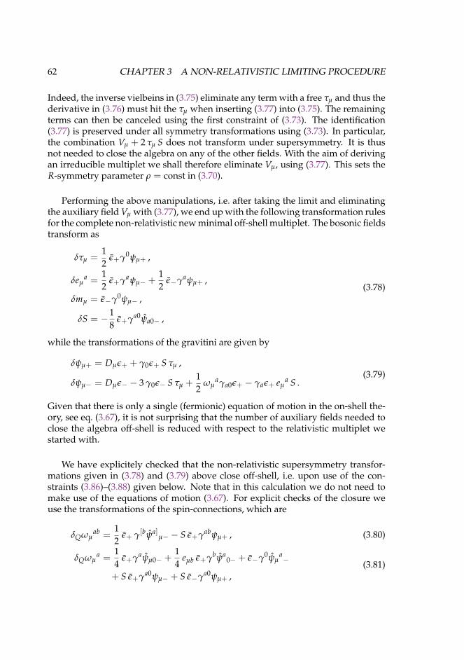
62 CHAPTER 3 A NON-RELATIVISTIC LIMITING PROCEDURE
Indeed, the inverse vielbeins in (3.75) eliminate any term with a free τµ and thus thederivative in (3.76) must hit the τµ when inserting (3.77) into (3.75). The remainingterms can then be canceled using the first constraint of (3.73). The identification(3.77) is preserved under all symmetry transformations using (3.73). In particular,the combination Vµ + 2 τµ S does not transform under supersymmetry. It is thusnot needed to close the algebra on any of the other fields. With the aim of derivingan irreducible multiplet we shall therefore eliminate Vµ, using (3.77). This sets theR-symmetry parameter ρ = const in (3.70).
Performing the above manipulations, i.e. after taking the limit and eliminatingthe auxiliary field Vµ with (3.77), we end up with the following transformation rulesfor the complete non-relativistic new minimal off-shell multiplet. The bosonic fieldstransform as
δτµ =12
ε+γ0ψµ+ ,
δeµa =
12
ε+γaψµ− +12
ε−γaψµ+ ,
δmµ = ε−γ0ψµ− ,
δS = −18
ε+γa0ψa0− ,
(3.78)
while the transformations of the gravitini are given by
δψµ+ = Dµε+ + γ0ε+ S τµ ,
δψµ− = Dµε− − 3 γ0ε− S τµ +12
ωµaγa0ε+ − γaε+ eµ
a S .(3.79)
Given that there is only a single (fermionic) equation of motion in the on-shell the-ory, see eq. (3.67), it is not surprising that the number of auxiliary fields needed toclose the algebra off-shell is reduced with respect to the relativistic multiplet westarted with.
We have explicitely checked that the non-relativistic supersymmetry transfor-mations given in (3.78) and (3.79) above close off-shell, i.e. upon use of the con-straints (3.86)–(3.88) given below. Note that in this calculation we do not need tomake use of the equations of motion (3.67). For explicit checks of the closure weuse the transformations of the spin-connections, which are
δQωµab =
12
ε+ γ[bψa]µ− − S ε+γabψµ+ , (3.80)
δQωµa =
14
ε+γaψµ0− +14
eµb ε+γbψa0− + ε−γ0ψµ
a−
+ S ε+γa0ψµ− + S ε−γa0ψµ+ ,(3.81)
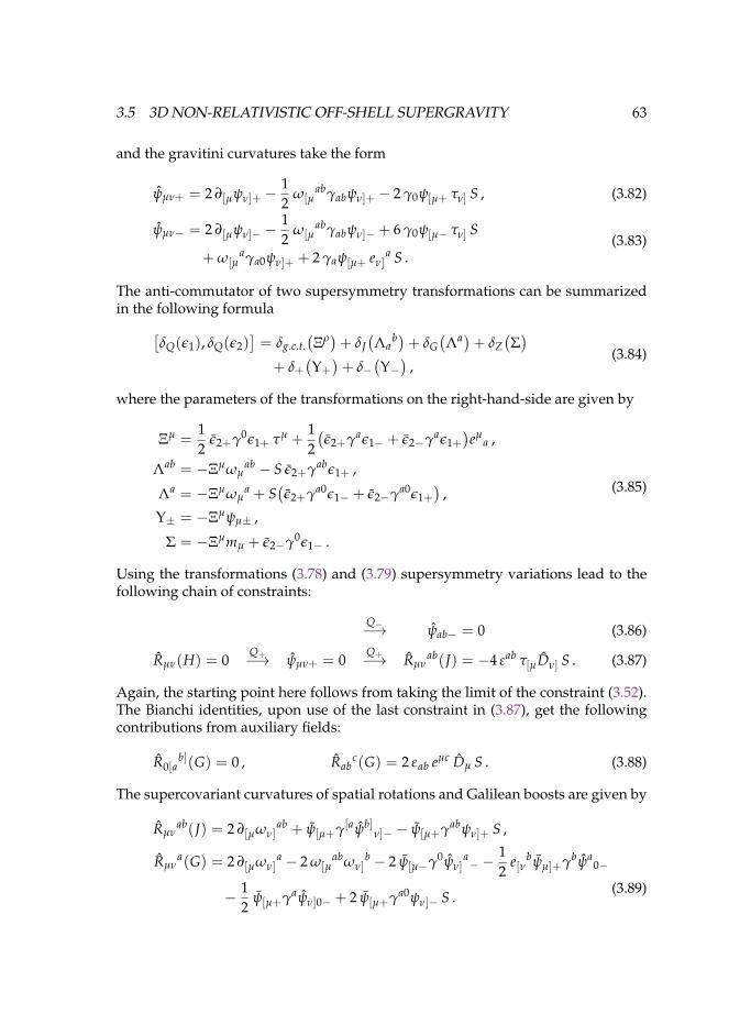
3.5 3D NON-RELATIVISTIC OFF-SHELL SUPERGRAVITY 63
and the gravitini curvatures take the form
ψµν+ = 2 ∂[µψν]+ −12
ω[µabγabψν]+ − 2 γ0ψ[µ+ τν] S , (3.82)
ψµν− = 2 ∂[µψν]− −12
ω[µabγabψν]− + 6 γ0ψ[µ− τν] S
+ ω[µaγa0ψν]+ + 2 γaψ[µ+ eν]
a S .(3.83)
The anti-commutator of two supersymmetry transformations can be summarizedin the following formula[
δQ(ε1), δQ(ε2)]= δg.c.t.
(Ξρ)+ δJ
(Λa
b)+ δG(Λa)+ δZ
(Σ)
+ δ+(Υ+)+ δ−
(Υ−)
,(3.84)
where the parameters of the transformations on the right-hand-side are given by
Ξµ =12
ε2+γ0ε1+ τµ +12(ε2+γaε1− + ε2−γaε1+
)eµ
a ,
Λab = −Ξµωµab − S ε2+γabε1+ ,
Λa = −Ξµωµa + S
(ε2+γa0ε1− + ε2−γa0ε1+
),
Υ± = −Ξµψµ± ,
Σ = −Ξµmµ + ε2−γ0ε1− .
(3.85)
Using the transformations (3.78) and (3.79) supersymmetry variations lead to thefollowing chain of constraints:
Q−−→ ψab− = 0 (3.86)
Rµν(H) = 0Q+−→ ψµν+ = 0
Q+−→ Rµνab(J) = −4 εab τ[µDν] S . (3.87)
Again, the starting point here follows from taking the limit of the constraint (3.52).The Bianchi identities, upon use of the last constraint in (3.87), get the followingcontributions from auxiliary fields:
R0[ab](G) = 0 , Rab
c(G) = 2 εab eµc Dµ S . (3.88)
The supercovariant curvatures of spatial rotations and Galilean boosts are given by
Rµνab(J) = 2 ∂[µων]
ab + ψ[µ+γ[aψb]ν]− − ψ[µ+γabψν]+ S ,
Rµνa(G) = 2 ∂[µων]
a − 2 ω[µabων]
b − 2 ψ[µ−γ0ψν]a− −
12
e[νbψµ]+γbψa
0−
− 12
ψ[µ+γaψν]0− + 2 ψ[µ+γa0ψν]− S .(3.89)
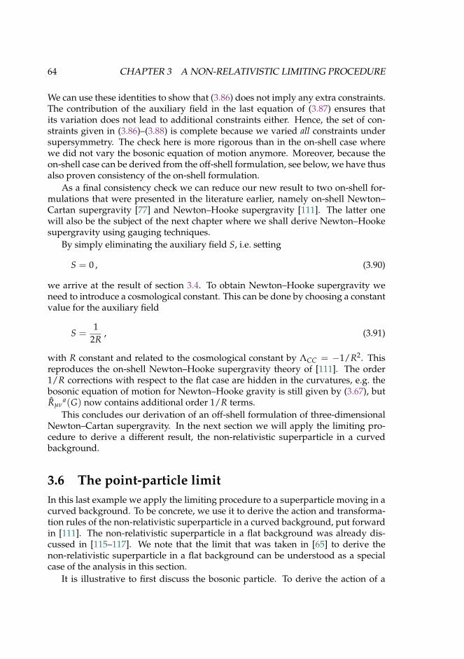
64 CHAPTER 3 A NON-RELATIVISTIC LIMITING PROCEDURE
We can use these identities to show that (3.86) does not imply any extra constraints.The contribution of the auxiliary field in the last equation of (3.87) ensures thatits variation does not lead to additional constraints either. Hence, the set of con-straints given in (3.86)–(3.88) is complete because we varied all constraints undersupersymmetry. The check here is more rigorous than in the on-shell case wherewe did not vary the bosonic equation of motion anymore. Moreover, because theon-shell case can be derived from the off-shell formulation, see below, we have thusalso proven consistency of the on-shell formulation.
As a final consistency check we can reduce our new result to two on-shell for-mulations that were presented in the literature earlier, namely on-shell Newton–Cartan supergravity [77] and Newton–Hooke supergravity [111]. The latter onewill also be the subject of the next chapter where we shall derive Newton–Hookesupergravity using gauging techniques.
By simply eliminating the auxiliary field S, i.e. setting
S = 0 , (3.90)
we arrive at the result of section 3.4. To obtain Newton–Hooke supergravity weneed to introduce a cosmological constant. This can be done by choosing a constantvalue for the auxiliary field
S =1
2R, (3.91)
with R constant and related to the cosmological constant by ΛCC = −1/R2. Thisreproduces the on-shell Newton–Hooke supergravity theory of [111]. The order1/R corrections with respect to the flat case are hidden in the curvatures, e.g. thebosonic equation of motion for Newton–Hooke gravity is still given by (3.67), butRµν
a(G) now contains additional order 1/R terms.This concludes our derivation of an off-shell formulation of three-dimensional
Newton–Cartan supergravity. In the next section we will apply the limiting pro-cedure to derive a different result, the non-relativistic superparticle in a curvedbackground.
3.6 The point-particle limitIn this last example we apply the limiting procedure to a superparticle moving in acurved background. To be concrete, we use it to derive the action and transforma-tion rules of the non-relativistic superparticle in a curved background, put forwardin [111]. The non-relativistic superparticle in a flat background was already dis-cussed in [115–117]. We note that the limit that was taken in [65] to derive thenon-relativistic superparticle in a flat background can be understood as a specialcase of the analysis in this section.
It is illustrative to first discuss the bosonic particle. To derive the action of a
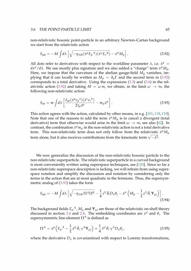
3.6 THE POINT-PARTICLE LIMIT 65
non-relativistic bosonic point-particle in an arbitrary Newton–Cartan backgroundwe start from the relativistic action
Srel = −M∫
dλ[√−ηAB(xµEµ
A)(xνEνB)− xµ Mµ
]. (3.92)
All dots refer to derivatives with respect to the worldline parameter λ, i.e. xµ =dxµ/dλ. We use mostly plus signature and we also added a “charge” term xµ Mµ.Here, we impose that the curvature of the abelian gauge-field Mµ vanishes, im-plying that it can locally be written as Mµ = ∂µΓ and the second term in (3.92)corresponds to a total derivative. Using the expressions (3.3) and (3.6) in the rel-ativistic action (3.92) and taking M = ω m, we obtain, in the limit ω → ∞, thefollowing non-relativistic action:
Snr = m∫
dλ
[δab(xµeµ
a)(xνeνb)
2τρ xρ −mµ xµ
]. (3.93)
This action agrees with the action, calculated by other means, in e.g. [101, 118, 119].Note that one of the reasons to add the term xµ Mµ is to cancel a divergent (totalderivative) term that otherwise would arise in the limit ω → ∞, see also [62]. Incontrast, the combination xµmµ in the non-relativistic action is not a total derivativeterm. This non-relativistic term does not only follow from the relativistic xµ Mµ
term alone, but it also receives contributions from the kinematic term√−x2.
We now generalize the discussion of the non-relativistic bosonic particle to thenon-relativistic superparticle. The relativistic superparticle in a curved backgroundis most conveniently written using superspace techniques, see [120]. Since so far anon-relativistic superspace description is lacking, we will refrain from using super-space notation and simplify the discussion and notation by considering only theterms in the action that are at most quadratic in the fermions. Thus, the supersym-metric analog of (3.92) takes the form
Srel = −M∫
dλ[√−ηAB ΠAΠB − 1
4εij θiDλθj − xµ
(Mµ −
12
εij θi Ψµj
)].
(3.94)
The background fields EµA, Mµ and Ψµi are those of the relativistic on-shell theory
discussed in section 3.4 and 2.8. The embedding coordinates are xµ and θi. Thesupersymmetric line-element ΠA is defined as
ΠA = xµ(
EµA − 1
2δij θi γAΨµj
)+
14
δij θi γADλθj , (3.95)
where the derivative Dλ is covariantized with respect to Lorentz transformations,
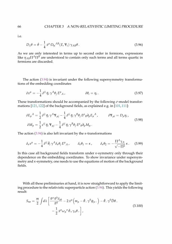
66 CHAPTER 3 A NON-RELATIVISTIC LIMITING PROCEDURE
i.e.
Dλθ = θ − 14
xµ ΩµAB(E, Ψi) γABθ . (3.96)
As we are only interested in terms up to second order in fermions, expressionslike ηABΠAΠB are understood to contain only such terms and all terms quartic infermions are discarded.
The action (3.94) is invariant under the following supersymmetry transforma-tions of the embedding coordinates
δxµ = −14
δij ηi γAθj EµA , δθi = ηi . (3.97)
These transformations should be accompanied by the following σ-model transfor-mations [121, 122] of the background fields, as explained e.g. in [101, 111]:
δEµA =
12
δij ηi γAΨµj −14
δij ηi γBθj EρB∂ρEµ
A , δΨµi = Dµηi ,
δMµ =12
εij ηi Ψµj −14
δij ηi γBθj EρB∂ρ Mµ .
(3.98)
The action (3.94) is also left invariant by the κ-transformations
δκxµ = −14
δij θi γAδκθj EµA , δκθ1 = κ , δκθ2 = − ΠAγA√
−Π2κ . (3.99)
In this case all background fields transform under κ-symmetry only through theirdependence on the embedding coordinates. To show invariance under supersym-metry and κ-symmetry, one needs to use the equations of motion of the backgroundfields.
With all these preliminaries at hand, it is now straightforward to apply the limit-ing procedure to the relativistic superparticle action (3.94). This yields the followingresult:
Snr =m2
∫dλ
[πaπbδab
π0 − 2 xµ(
mµ − θ−γ0ψµ−)− θ−γ0Dθ−
− 12
xµωµa θ+γaθ−
],
(3.100)

3.6 THE POINT-PARTICLE LIMIT 67
where we have defined the following supersymmetric line-elements
π0 = xµ(
τµ −12
θ+γ0ψµ+
)+
14
θ+γ0Dθ+ , (3.101)
πa = xµ(
eµa − 1
2θ+γaψµ− −
12
θ−γaψµ+
)+
14
θ+γaDθ− +14
θ−γaDθ+
+18
θ+γaγb0θ+ xµωµb .
(3.102)
Note that the supercovariant derivative D is covariant with respect to spatial rota-tions, not boosts. The boost-connection ωµ
a that appears in eqs. (3.100) and (3.102)is the dependent boost-connection (3.61). For notational simplicity we do not de-note below its dependence on the other fields. The transformations of the embed-ding coordinates under κ-symmetry are given by
δt = −14
θ+γ0κ , δθ+ = κ ,
δxi = −14
θ−γiκ − 18
π j
π0 θ+γ0iγjκ , δθ− = − πi
2π0 γi0κ .(3.103)
This reproduces precisely, to second order in fermions, the κ-symmetric non-relativ-istic superparticle in a curved background as presented in [111]. Fixing κ-symmetryby setting θ+ = 0 leads to the result of [111]. When we gauge-fix the Newton–Cartan background to a Galilean background with a Newton potential Φ, the onedescribed in [77], the action (3.100) reduces to
Snr =m2
∫dλ
[πi
ΦπiΦ
π0 − 2 t(Φ− θ−γ0Ψ
)− θ−γ0θ− +
t2
∂iΦ θ+γiθ−
], (3.104)
with the “super-Galilean” line-elements given by
π0 = t +14
θ+γ0θ+ , (3.105)
πiΦ = xi − 1
2t θ+γiΨ +
14
θ+γi θ− +14
θ−γi θ+ −18
t ∂jΦ θ+γiγj0θ+ . (3.106)
This finishes our discussion of the superparticle in a non-relativistic curved back-ground. We have shown that the limiting procedure can be applied to also obtainresults different from gravitational backgrounds. In the next section we present ashort recap of this chapter and give an outlook on possible further applications ofthe limiting procedure that we have developed.
68 CHAPTER 3 A NON-RELATIVISTIC LIMITING PROCEDURE
3.7 ConclusionIn this chapter we have established a procedure to derive a non-relativistic theoryof supergravity from a relativistic one. Our ansatz is strongly motivated by the con-traction of relativistic symmetry algebras to non-relativistic ones. This contractiondetermines the scaling of all gauge-fields. Usually, the easiest part then is to findthe transformation rules of the independent non-relativistic gauge-fields. These canbe compared to the transformations rules that we would find had we started outby gauging the non-relativistic symmetry algebra directly.
One non-trivial aspect of the procedure consists of finding the correct set ofconstraints. For example, in order to avoid divergences we need to set to zero someof the curvatures of the gauge-fields like e.g. Fµν(M) = 0. Here, the difficulty lies infinding a complete set of constraints, such that we eliminate not only the divergentterms, but also all their putative, finite contributions in the commutator algebra.The chains of constraints (3.65)–(3.67) and (3.86)–(3.87) comprise such complete setsof constraints.
Also, as we established in the explicit exercise in section 3.4, it is not alwaysstraightforward to find all the equations of motion by taking the non-relativisticlimit of the relativistic equation of motion. For example, the equations (3.67) do notfollow from a non-relativistic limit of the relativistic equations of motion. We wereable though to find the non-relativistic equation of motion by varying all constraintsunder supersymmetry.
In our last example we took the non-relativistic limit of a point-particle thatmoves in an arbitrary dynamical supergravity background. The aim of this analysiswas to perform yet another check of the procedure, by deriving the results of [111],and also to show that the limit works on theories other than pure (super)gravity.
As hopefully made clear by the examples in this chapter, our procedure does notjust consist of taking a limit. We also have to impose constraints and sometimeseliminate fields. In this sense it is a truncation as much as a limit. Therefore weprefer to refer to it as the “non-relativistic limiting procedure” rather than the “non-relativistic limit”. Simply calling it a non-relativistic limit certainly also causes con-fusion with previous works in the literature.
Many different such non-relativistic limits have been put forward in the litera-ture, including supersymmetric theories, see e.g. [13, 16, 90, 91, 118, 123, 124]. How-ever, none of them quite compares to our limit because they do not make this sys-tematic use of the contraction of symmetry algebras.
Our hope is that this new way of thinking about the non-relativistic limit enablesus not only to re-derive known results, as we mainly did in this chapter, but alsoto use the limit to get novel non-relativistic (supergravity) theories, like in section3.5. For example, in chapter 6 we make use of this procedure to derive novel non-relativistic matter multiplets.
In chapter 2, see section 2.5.4, we already mentioned the issue of taking thelimit in three space-time dimensions. Very similar structures appear in the super-
3.7 CONCLUSION 69
symmetric case as well, i.e. in the limit a relativistic source cannot yield any (source)contribution on the right-hand-side of the equation of motion (3.67).
Note that we did not look at the non-relativistic limit of electrodynamics in thischapter. This is an interesting extension as there exists more than one limit in thiscase [125]. This has to do with the fact that we only consider c → ∞ here, where cis the speed of light. In electrodynamics c is related to two “coupling constants” ε0and µ0 via ε0µ0 = 1/c2. Sending c → ∞ yields ε0µ0 → 0, but we can still choosewhich of the two vanishes. This leads to an “electric” and a “magnetic” limit whichlead to different non-relativistic theories.
A worthwhile exercise might be to apply this procedure to the four-dimensionalsupergravity multiplet. Ideally, this leads to a four-dimensional Newton–Cartansupergravity theory, which has not been found so far. However, our procedure isnot bound to lead to a result, unless one chooses the correct starting point. In partic-ular, without the correct constraints that allow one to get rid of putative divergentterms, such as e.g. Fµν(M) = 0 in our examples, the procedure will not yield a goodresult. That is not to say that four-dimensional Newton–Cartan supergravity doesnot exist, but a bit of trial and error might be needed to find the correct startingpoint.
There also exist other, for example ultra-relativistic contractions of symmetryalgebras. Having a limiting procedure that depends only on the contraction itself,but not the fact that it is a non-relativistic contraction, means that we should beable to generalize the procedure and apply it to derive an ultra-relativistic Carrollgravity [61] as well and to derive Carroll (super)particle actions such as those givenin [59, 60].
We will come back to this in the last chapter of this thesis where we also aim togive a more detailed outlook on possible applications of our (not necessarily non-relativistic) limiting procedure.


4Newton–Hooke supergravity
In this chapter we will derive a cosmological extension of non-relativistic su-pergravity. To obtain this theory, Newton–Hooke supergravity, we will usegauging techniques, like we discussed in chapter 2. To do so, we need theNewton–Hooke superalgebra, which we derive in section 4.1. Then, we derivenon-relativistic supergravity on cosmological space-time manifolds, i.e. with anon-vanishing cosmological constant, in section 4.2. We proceed to discuss aparticular gauge-fixing to obtain a Galilean version of Newton–Hooke super-gravity in section 4.3. In section 4.4, we discuss how the results of this chapterare related to their relativistic counterpart, anti-de Sitter supergravity, throughthe non-relativistic limiting procedure introduced in chapter 3.
72 CHAPTER 4 NEWTON–HOOKE SUPERGRAVITY
This chapter is largely based on the construction of Newton–Cartan supergravityin [77]. Here, we will perform a similar analysis for a slightly more general case byincluding a negative cosmological constant ΛCC = −1/R2. Of course, all formulasthat we obtain in this chapter must reduce to those of Newton–Cartan supergravityin the limit R → ∞. This always serves as a quick check on the results that we areabout to derive.
Given that there are no actions for non-relativistic (super)gravity theories, gaug-ing procedures so far were the only way to construct, and understand, such the-ories. This is why, in this chapter, we start out by constructing this new non-relativistic supergravity theory in precisely that way. The analysis proceeds alongsimilar lines as we saw in chapter 2, when we showed how general relativity can beconstructed by gauging the Poincare algebra. In this chapter, we will gauge a non-relativistic superalgebra, the Newton–Hooke superalgebra. The bosonic version ofthis algebra can be derived from the (anti-)de Sitter algebra by an Inonu–Wignercontraction [126]. For more works on Newton–Hooke algebras and space-times seee.g. [127–132] and supersymmetric extensions can be found e.g. in [133–135]. Here,we will derive the superalgebra ourselves by a non-relativistic contraction of ananti-de Sitter superalgebra. To show how this contraction works on the algebra isimportant when we want to take the limit of the supergravity fields later.
The gauging of the Newton–Hooke superalgebra will lead to a theory withmany, in some sense too many, symmetries. Like in the relativistic case we will im-pose curvature constraints, see also [77]. It will then be possible to solve for someof the gauge-fields explicitely. We will also consider a partial gauge-fixing, wherewe use some of the curvature constraints to fix particular values of the gauge-fields,i.e. to eliminate some of their components. We will make maximal use of this to de-rive a Galilean version of Newton–Hooke supergravity, i.e. a supergravity theoryof a Galilean observer. This Galilean observer is living on a space-time manifoldwhich is curved due to the presence of a cosmological constant. In this special sce-nario space-time is curved, but space is flat, i.e. Rµν
ab(J) = 0. In the end, we willrelate the theory that we construct here to a relativistic one via the non-relativisticlimiting procedure introduced in the previous chapter.
We have no prove that the limit must always lead to the same theory that wewould get from gauging. Hence, this chapter also serves as a check on the non-relativistic contraction itself. In particular, we will derive the same novel super-gravity theory in two different ways, via gauging and via the limiting procedure.For that purpose, let us recall the figure 1.1 that we used in the introduction. Asimilar diagram may serve as the motivation for the current chapter, see figure 4.1.The aim of this chapter is thus to show that the gravitational theories obtained bygauging the Newton–Hooke (super)algebra coincide with the theories that followfrom taking the non-relativistic limit of anti-de Sitter (super)gravity.
This chapter is organized as follows. In section 4.1 we derive the Newton–Hooke (super)algebra. Then we proceed to gauge it to get Newton–Hooke su-pergravity in section 4.2. Section 4.3 deals with a particular gauge-fixing of theNewton–Hooke supergravity background. In section 4.4 we use the contraction of
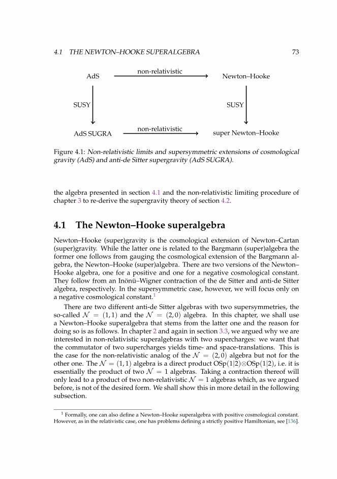
4.1 THE NEWTON–HOOKE SUPERALGEBRA 73
AdS
AdS SUGRA
Newton–Hooke
super Newton–Hooke
SUSY SUSY
non-relativistic
non-relativistic
Figure 4.1: Non-relativistic limits and supersymmetric extensions of cosmologicalgravity (AdS) and anti-de Sitter supergravity (AdS SUGRA).
the algebra presented in section 4.1 and the non-relativistic limiting procedure ofchapter 3 to re-derive the supergravity theory of section 4.2.
4.1 The Newton–Hooke superalgebraNewton–Hooke (super)gravity is the cosmological extension of Newton–Cartan(super)gravity. While the latter one is related to the Bargmann (super)algebra theformer one follows from gauging the cosmological extension of the Bargmann al-gebra, the Newton–Hooke (super)algebra. There are two versions of the Newton–Hooke algebra, one for a positive and one for a negative cosmological constant.They follow from an Inonu–Wigner contraction of the de Sitter and anti-de Sitteralgebra, respectively. In the supersymmetric case, however, we will focus only ona negative cosmological constant.1
There are two different anti-de Sitter algebras with two supersymmetries, theso-called N = (1, 1) and the N = (2, 0) algebra. In this chapter, we shall usea Newton–Hooke superalgebra that stems from the latter one and the reason fordoing so is as follows. In chapter 2 and again in section 3.3, we argued why we areinterested in non-relativistic superalgebras with two supercharges: we want thatthe commutator of two supercharges yields time- and space-translations. This isthe case for the non-relativistic analog of the N = (2, 0) algebra but not for theother one. The N = (1, 1) algebra is a direct product OSp(1|2)⊗OSp(1|2), i.e. it isessentially the product of two N = 1 algebras. Taking a contraction thereof willonly lead to a product of two non-relativistic N = 1 algebras which, as we arguedbefore, is not of the desired form. We shall show this in more detail in the followingsubsection.
1 Formally, one can also define a Newton–Hooke superalgebra with positive cosmological constant.However, as in the relativistic case, one has problems defining a strictly positive Hamiltonian, see [136].
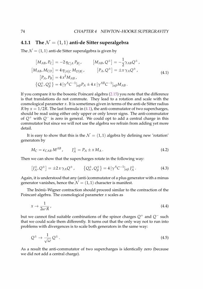
74 CHAPTER 4 NEWTON–HOOKE SUPERGRAVITY
4.1.1 The N = (1, 1) anti-de Sitter superalgebra
The N = (1, 1) anti-de Sitter superalgebra is given by
[MAB, PC
]= −2 ηC[A PB] ,
[MAB, Q±
]= −1
2γABQ± ,[
MAB, MCD]= 4 η[A[C MD]B] ,
[PA, Q±
]= ±x γAQ± ,[
PA, PB]= 4 x2MAB ,
Q±α , Q±β= 4 [γAC−1]αβPA ± 4 x [γABC−1]αβ MAB .
(4.1)
If you compare it to the bosonic Poincare algebra (2.15) you note that the differenceis that translations do not commute. They lead to a rotation and scale with thecosmological parameter x. It is sometimes given in terms of the anti-de Sitter radiusR by x = 1/2R. The last formula in (4.1), the anti-commutator of two supercharges,should be read using either only upper or only lower signs. The anti-commutatorof Q+ with Q− is zero in general. We could opt to add a central charge in thiscommutator but since we will not use the algebra we refrain from adding yet moredetail.
It is easy to show that this is the N = (1, 1) algebra by defining new ’rotation’generators by
MC = εCAB MAB , J±A = PA ± x MA . (4.2)
Then we can show that the supercharges rotate in the following way:[J±A , Q±
]= ±2 x γAQ± ,
Q±α , Q±β
= 4 [γAC−1]αβ J±A . (4.3)
Again, it is understood that any (anti-)commutator of a plus generator with a minusgenerator vanishes, hence the N = (1, 1) character is manifest.
The Inonu–Wigner contraction should proceed similar to the contraction of thePoincare algebra. The cosmological parameter x scales as
x → 12ω R
, (4.4)
but we cannot find suitable combinations of the spinor charges Q+ and Q− suchthat we could scale them differently. It turns out that the only way not to run intoproblems with divergences is to scale both generators in the same way:
Q± → 1√ω
Q± . (4.5)
As a result the anti-commutator of two supercharges is identically zero (becausewe did not add a central charge).
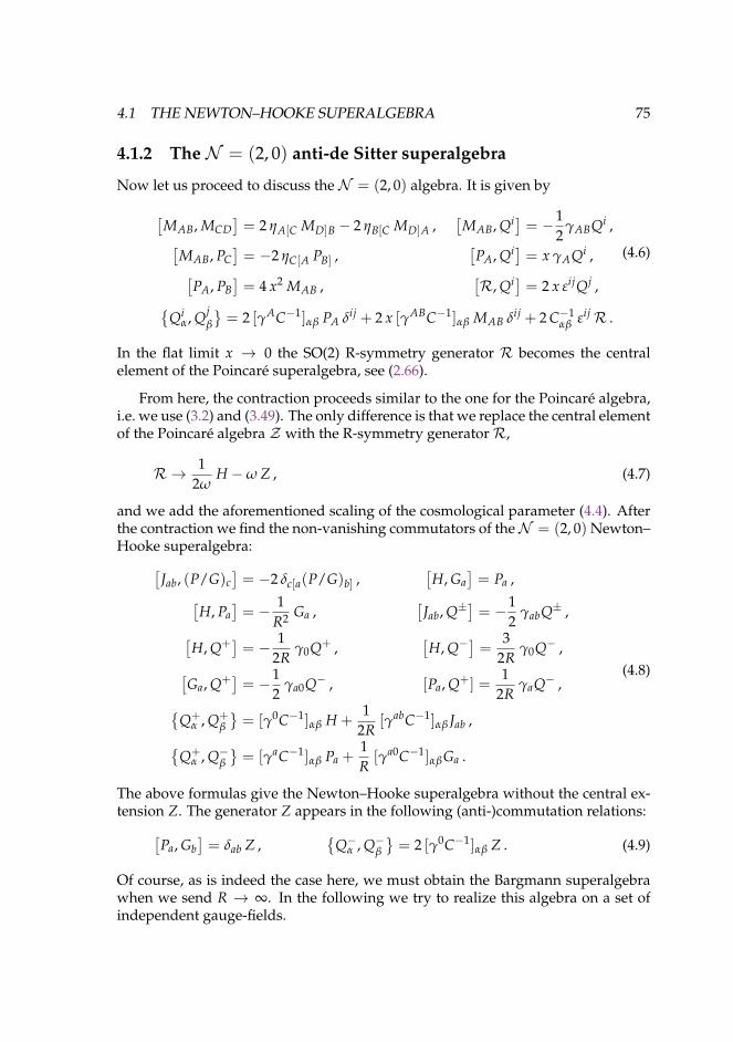
4.1 THE NEWTON–HOOKE SUPERALGEBRA 75
4.1.2 The N = (2, 0) anti-de Sitter superalgebra
Now let us proceed to discuss the N = (2, 0) algebra. It is given by
[MAB, MCD
]= 2 ηA[C MD]B − 2 ηB[C MD]A ,
[MAB, Qi] = −1
2γABQi ,[
MAB, PC]= −2 ηC[A PB] ,
[PA, Qi] = x γAQi ,[
PA, PB]= 4 x2 MAB ,
[R, Qi] = 2 x εijQj ,
(4.6)
Qi
α, Qjβ
= 2 [γAC−1]αβ PA δij + 2 x [γABC−1]αβ MAB δij + 2 C−1
αβ εijR .
In the flat limit x → 0 the SO(2) R-symmetry generator R becomes the centralelement of the Poincare superalgebra, see (2.66).
From here, the contraction proceeds similar to the one for the Poincare algebra,i.e. we use (3.2) and (3.49). The only difference is that we replace the central elementof the Poincare algebra Z with the R-symmetry generatorR,
R → 12ω
H −ω Z , (4.7)
and we add the aforementioned scaling of the cosmological parameter (4.4). Afterthe contraction we find the non-vanishing commutators of theN = (2, 0) Newton–Hooke superalgebra:[
Jab, (P/G)c]= −2 δc[a(P/G)b] ,
[H, Ga
]= Pa ,[
H, Pa]= − 1
R2 Ga ,[
Jab, Q±]= −1
2γabQ± ,[
H, Q+]= − 1
2Rγ0Q+ ,
[H, Q−
]=
32R
γ0Q− ,[Ga, Q+
]= −1
2γa0Q− , [Pa, Q+] =
12R
γaQ− ,Q+
α , Q+β
= [γ0C−1]αβ H +
12R
[γabC−1]αβ Jab ,Q+
α , Q−β= [γaC−1]αβ Pa +
1R[γa0C−1]αβGa .
(4.8)
The above formulas give the Newton–Hooke superalgebra without the central ex-tension Z. The generator Z appears in the following (anti-)commutation relations:[
Pa, Gb]= δab Z ,
Q−α , Q−β
= 2 [γ0C−1]αβ Z . (4.9)
Of course, as is indeed the case here, we must obtain the Bargmann superalgebrawhen we send R → ∞. In the following we try to realize this algebra on a set ofindependent gauge-fields.
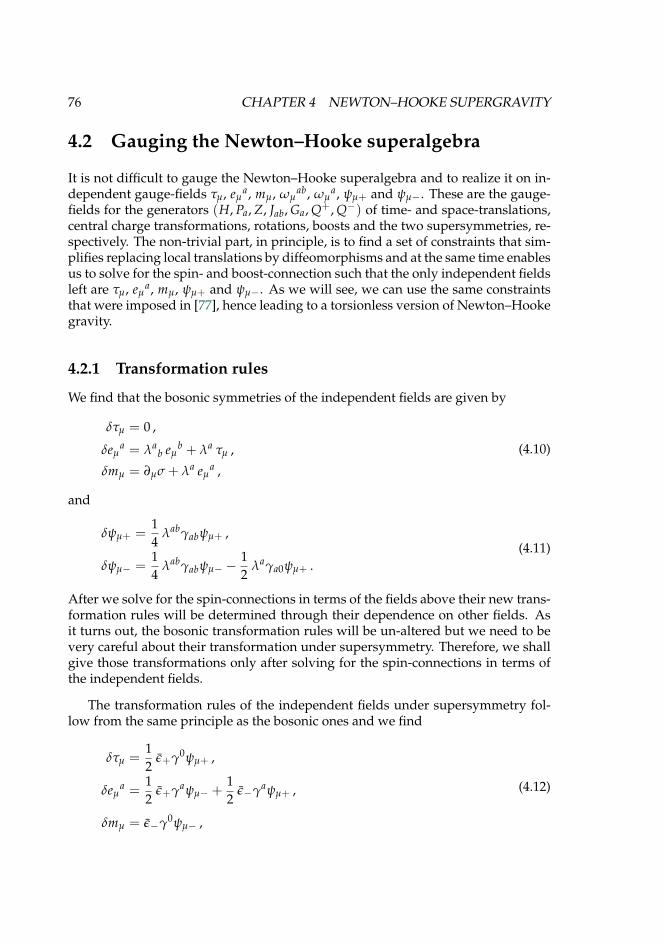
76 CHAPTER 4 NEWTON–HOOKE SUPERGRAVITY
4.2 Gauging the Newton–Hooke superalgebra
It is not difficult to gauge the Newton–Hooke superalgebra and to realize it on in-dependent gauge-fields τµ, eµ
a, mµ, ωµab, ωµ
a, ψµ+ and ψµ−. These are the gauge-fields for the generators (H, Pa, Z, Jab, Ga, Q+, Q−) of time- and space-translations,central charge transformations, rotations, boosts and the two supersymmetries, re-spectively. The non-trivial part, in principle, is to find a set of constraints that sim-plifies replacing local translations by diffeomorphisms and at the same time enablesus to solve for the spin- and boost-connection such that the only independent fieldsleft are τµ, eµ
a, mµ, ψµ+ and ψµ−. As we will see, we can use the same constraintsthat were imposed in [77], hence leading to a torsionless version of Newton–Hookegravity.
4.2.1 Transformation rules
We find that the bosonic symmetries of the independent fields are given by
δτµ = 0 ,
δeµa = λa
b eµb + λa τµ ,
δmµ = ∂µσ + λa eµa ,
(4.10)
and
δψµ+ =14
λabγabψµ+ ,
δψµ− =14
λabγabψµ− −12
λaγa0ψµ+ .(4.11)
After we solve for the spin-connections in terms of the fields above their new trans-formation rules will be determined through their dependence on other fields. Asit turns out, the bosonic transformation rules will be un-altered but we need to bevery careful about their transformation under supersymmetry. Therefore, we shallgive those transformations only after solving for the spin-connections in terms ofthe independent fields.
The transformation rules of the independent fields under supersymmetry fol-low from the same principle as the bosonic ones and we find
δτµ =12
ε+γ0ψµ+ ,
δeµa =
12
ε+γaψµ− +12
ε−γaψµ+ ,
δmµ = ε−γ0ψµ− ,
(4.12)
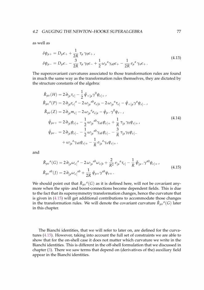
4.2 GAUGING THE NEWTON–HOOKE SUPERALGEBRA 77
as well as
δψµ+ = Dµε+ +1
2Rτµ γ0ε+ ,
δψµ− = Dµε− −3
2Rτµ γ0ε− +
12
ωµaγa0ε+ −
12R
eµa γaε+ .
(4.13)
The supercovariant curvatures associated to those transformation rules are foundin much the same way as the transformation rules themselves, they are dictated bythe structure constants of the algebra:
Rµν(H) = 2 ∂[µτν] −12
ψ+[µγ0ψν]+ ,
Rµνa(P) = 2 ∂[µeν]
a − 2 ω[µabeν]b − 2 ω[µ
aτν] − ψ+[µγaψν]− ,
Rµν(Z) = 2 ∂[µmν] − 2 ω[µaeν]a − ψµ−γ0ψν− ,
ψµν+ = 2 ∂[µψν]+ −12
ω[µabγabψν]+ +
1R
τ[µ γ0ψν]+ ,
ψµν− = 2 ∂[µψν]− −12
ω[µabγabψν]− −
3R
τ[µγ0ψν]−
+ ω[µaγa0ψν]+ −
1R
e[µaγaψν]+ .
(4.14)
and
Rµνa(G) = 2 ∂[µων]
a − 2 ω[µabων]b +
2R2 e[µ
aτν] −1R
ψ[µ−γa0ψν]+ ,
Rµνab(J) = 2 ∂[µων]
ab +1
2Rψµ+γabψν+ .
(4.15)
We should point out that Rµνa(G) as it is defined here, will not be covariant any-
more when the spin- and boost-connections become dependent fields. This is dueto the fact that its supersymmetry transformation changes, hence the curvature thatis given in (4.15) will get additional contributions to accommodate those changesin the transformation rules. We will denote the covariant curvature Rµν
a(G) laterin this chapter.
The Bianchi identities, that we will refer to later on, are defined for the curva-tures (4.15). However, taking into account the full set of constraints we are able toshow that for the on-shell case it does not matter which curvature we write in theBianchi identities. This is different in the off-shell formulation that we discussed inchapter (3). There we saw terms that depend on (derivatives of the) auxiliary fieldappear in the Bianchi identities.
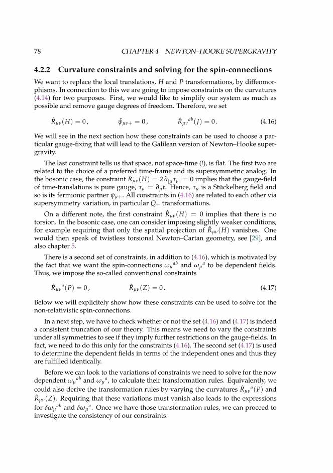
78 CHAPTER 4 NEWTON–HOOKE SUPERGRAVITY
4.2.2 Curvature constraints and solving for the spin-connectionsWe want to replace the local translations, H and P transformations, by diffeomor-phisms. In connection to this we are going to impose constraints on the curvatures(4.14) for two purposes. First, we would like to simplify our system as much aspossible and remove gauge degrees of freedom. Therefore, we set
Rµν(H) = 0 , ψµν+ = 0 , Rµνab(J) = 0 . (4.16)
We will see in the next section how these constraints can be used to choose a par-ticular gauge-fixing that will lead to the Galilean version of Newton–Hooke super-gravity.
The last constraint tells us that space, not space-time (!), is flat. The first two arerelated to the choice of a preferred time-frame and its supersymmetric analog. Inthe bosonic case, the constraint Rµν(H) = 2 ∂[µτν] = 0 implies that the gauge-fieldof time-translations is pure gauge, τµ = ∂µt. Hence, τµ is a Stuckelberg field andso is its fermionic partner ψµ+. All constraints in (4.16) are related to each other viasupersymmetry variation, in particular Q+ transformations.
On a different note, the first constraint Rµν(H) = 0 implies that there is notorsion. In the bosonic case, one can consider imposing slightly weaker conditions,for example requiring that only the spatial projection of Rµν(H) vanishes. Onewould then speak of twistless torsional Newton–Cartan geometry, see [29], andalso chapter 5.
There is a second set of constraints, in addition to (4.16), which is motivated bythe fact that we want the spin-connections ωµ
ab and ωµa to be dependent fields.
Thus, we impose the so-called conventional constraints
Rµνa(P) = 0 , Rµν(Z) = 0 . (4.17)
Below we will explicitely show how these constraints can be used to solve for thenon-relativistic spin-connections.
In a next step, we have to check whether or not the set (4.16) and (4.17) is indeeda consistent truncation of our theory. This means we need to vary the constraintsunder all symmetries to see if they imply further restrictions on the gauge-fields. Infact, we need to do this only for the constraints (4.16). The second set (4.17) is usedto determine the dependent fields in terms of the independent ones and thus theyare fulfilled identically.
Before we can look to the variations of constraints we need to solve for the nowdependent ωµ
ab and ωµa, to calculate their transformation rules. Equivalently, we
could also derive the transformation rules by varying the curvatures Rµνa(P) and
Rµν(Z). Requiring that these variations must vanish also leads to the expressionsfor δωµ
ab and δωµa. Once we have those transformation rules, we can proceed to
investigate the consistency of our constraints.
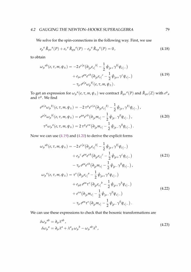
4.2 GAUGING THE NEWTON–HOOKE SUPERALGEBRA 79
We solve for the spin-connections in the following way. First, we use
eρa Rµν
a(P) + eνa Rρµ
a(P)− eµa Rνρ
a(P) = 0 , (4.18)
to obtain
ωµab(e, τ, m, ψ±) = −2 eν[a(∂[µeν]
b] − 12
ψ[µ+γb]ψν]−)
+ eµc eρaeνb(∂[µeν]c − 1
2ψ[µ+γcψν]−
)− τµ eρ[aωρ
b](e, τ, m, ψ±) .
(4.19)
To get an expression for ωµa(e, τ, m, ψ±) we contract Rµν
a(P) and Rµν(Z) with eµa
and τµ. We find
eµ(aωµb)(e, τ, m, ψ±) = −2 τµeν(a(∂[µeν]
b) − 12
ψ[µ+γb)ψν]−)
,
eµ[aωµb](e, τ, m, ψ±) = eµaeνb(∂[µmν] −
12
ψ[µ−γ0ψν]−)
,
τµωµa(e, τ, m, ψ±) = 2 τµeνa(∂[µmν] −
12
ψ[µ−γ0ψν]−)
.
(4.20)
Now we can use (4.19) and (4.20) to derive the explicit forms
ωµab(e, τ, m, ψ±) = −2 eν[a(∂[µeν]
b] − 12
ψ[µ+γb]ψν]−)
+ eµc eρaeνb(∂[ρeν]
c − 12
ψ[ρ+γcψν]−)
− τµ eρaeνb(∂[ρmν] −12
ψ[ρ−γ0ψν]−)
,
(4.21)
ωµa(e, τ, m, ψ±) = τν
(∂[µeν]
a − 12
ψ[µ+γaψν]−)
+ eµb eρaτν(∂[ρeν]
b − 12
ψ[ρ+γbψν]−)
+ eνa(∂[µmν] −12
ψ[µ−γ0ψν]−)
− τµ eρaτν(∂[ρmν] −
12
ψ[ρ−γ0ψν]−)
.
(4.22)
We can use these expressions to check that the bosonic transformations are
δωµab = ∂µλab ,
δωµa = ∂µλa + λa
b ωµb −ωµ
abλb ,(4.23)
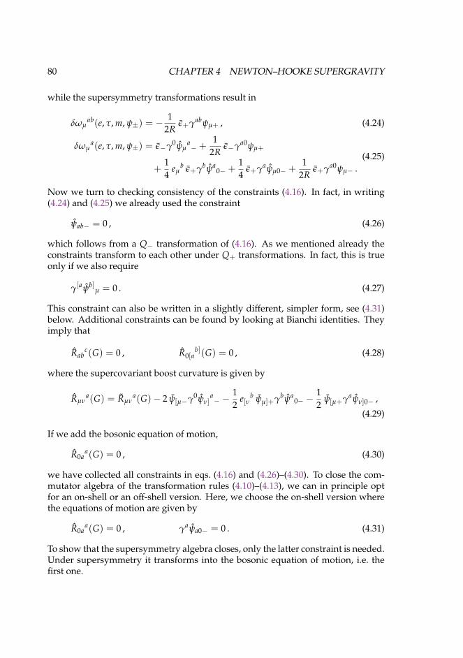
80 CHAPTER 4 NEWTON–HOOKE SUPERGRAVITY
while the supersymmetry transformations result in
δωµab(e, τ, m, ψ±) = −
12R
ε+γabψµ+ , (4.24)
δωµa(e, τ, m, ψ±) = ε−γ0ψµ
a− +
12R
ε−γa0ψµ+
+14
eµb ε+γbψa
0− +14
ε+γaψµ0− +1
2Rε+γa0ψµ− .
(4.25)
Now we turn to checking consistency of the constraints (4.16). In fact, in writing(4.24) and (4.25) we already used the constraint
ψab− = 0 , (4.26)
which follows from a Q− transformation of (4.16). As we mentioned already theconstraints transform to each other under Q+ transformations. In fact, this is trueonly if we also require
γ[aψb]µ = 0 . (4.27)
This constraint can also be written in a slightly different, simpler form, see (4.31)below. Additional constraints can be found by looking at Bianchi identities. Theyimply that
Rabc(G) = 0 , R0[a
b](G) = 0 , (4.28)
where the supercovariant boost curvature is given by
Rµνa(G) = Rµν
a(G)− 2 ψ[µ−γ0ψν]a− −
12
e[νb ψµ]+γbψa
0− −12
ψ[µ+γaψν]0− ,
(4.29)
If we add the bosonic equation of motion,
R0aa(G) = 0 , (4.30)
we have collected all constraints in eqs. (4.16) and (4.26)–(4.30). To close the com-mutator algebra of the transformation rules (4.10)–(4.13), we can in principle optfor an on-shell or an off-shell version. Here, we choose the on-shell version wherethe equations of motion are given by
R0aa(G) = 0 , γaψa0− = 0 . (4.31)
To show that the supersymmetry algebra closes, only the latter constraint is needed.Under supersymmetry it transforms into the bosonic equation of motion, i.e. thefirst one.
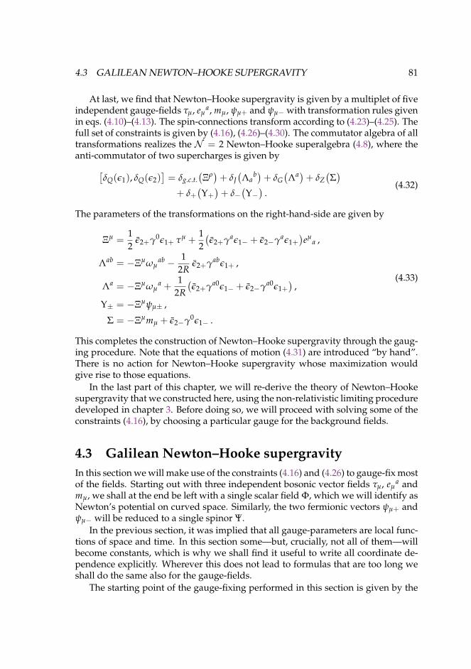
4.3 GALILEAN NEWTON–HOOKE SUPERGRAVITY 81
At last, we find that Newton–Hooke supergravity is given by a multiplet of fiveindependent gauge-fields τµ, eµ
a, mµ, ψµ+ and ψµ− with transformation rules givenin eqs. (4.10)–(4.13). The spin-connections transform according to (4.23)–(4.25). Thefull set of constraints is given by (4.16), (4.26)–(4.30). The commutator algebra of alltransformations realizes the N = 2 Newton–Hooke superalgebra (4.8), where theanti-commutator of two supercharges is given by[
δQ(ε1), δQ(ε2)]= δg.c.t.
(Ξρ)+ δJ
(Λa
b)+ δG(Λa)+ δZ
(Σ)
+ δ+(Υ+)+ δ−
(Υ−)
.(4.32)
The parameters of the transformations on the right-hand-side are given by
Ξµ =12
ε2+γ0ε1+ τµ +12(ε2+γaε1− + ε2−γaε1+
)eµ
a ,
Λab = −Ξµωµab − 1
2Rε2+γabε1+ ,
Λa = −Ξµωµa +
12R(ε2+γa0ε1− + ε2−γa0ε1+
),
Υ± = −Ξµψµ± ,
Σ = −Ξµmµ + ε2−γ0ε1− .
(4.33)
This completes the construction of Newton–Hooke supergravity through the gaug-ing procedure. Note that the equations of motion (4.31) are introduced “by hand”.There is no action for Newton–Hooke supergravity whose maximization wouldgive rise to those equations.
In the last part of this chapter, we will re-derive the theory of Newton–Hookesupergravity that we constructed here, using the non-relativistic limiting proceduredeveloped in chapter 3. Before doing so, we will proceed with solving some of theconstraints (4.16), by choosing a particular gauge for the background fields.
4.3 Galilean Newton–Hooke supergravityIn this section we will make use of the constraints (4.16) and (4.26) to gauge-fix mostof the fields. Starting out with three independent bosonic vector fields τµ, eµ
a andmµ, we shall at the end be left with a single scalar field Φ, which we will identify asNewton’s potential on curved space. Similarly, the two fermionic vectors ψµ+ andψµ− will be reduced to a single spinor Ψ.
In the previous section, it was implied that all gauge-parameters are local func-tions of space and time. In this section some—but, crucially, not all of them—willbecome constants, which is why we shall find it useful to write all coordinate de-pendence explicitly. Wherever this does not lead to formulas that are too long weshall do the same also for the gauge-fields.
The starting point of the gauge-fixing performed in this section is given by the
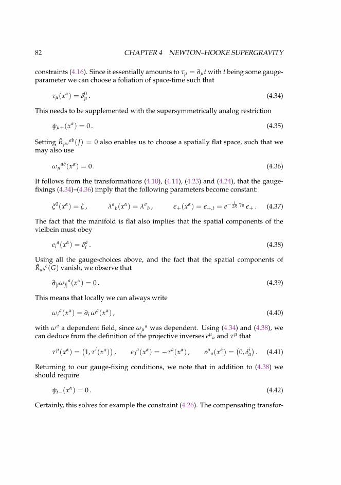
82 CHAPTER 4 NEWTON–HOOKE SUPERGRAVITY
constraints (4.16). Since it essentially amounts to τµ = ∂µt with t being some gauge-parameter we can choose a foliation of space-time such that
τµ(xα) = δ0µ . (4.34)
This needs to be supplemented with the supersymmetrically analog restriction
ψµ+(xα) = 0 . (4.35)
Setting Rµνab(J) = 0 also enables us to choose a spatially flat space, such that we
may also use
ωµab(xα) = 0 . (4.36)
It follows from the transformations (4.10), (4.11), (4.23) and (4.24), that the gauge-fixings (4.34)–(4.36) imply that the following parameters become constant:
ξ0(xα) = ζ , λab(xα) = λa
b , ε+(xα) = ε+,t = e−t
2R γ0 ε+ . (4.37)
The fact that the manifold is flat also implies that the spatial components of thevielbein must obey
eia(xα) = δa
i . (4.38)
Using all the gauge-choices above, and the fact that the spatial components ofRab
c(G) vanish, we observe that
∂[iωj]a(xα) = 0 . (4.39)
This means that locally we can always write
ωia(xα) = ∂i ωa(xα) , (4.40)
with ωa a dependent field, since ωµa was dependent. Using (4.34) and (4.38), we
can deduce from the definition of the projective inverses eµa and τµ that
τµ(xα) =(1, τi(xα)
), e0
a(xα) = −τa(xα) , eµa(xα) =
(0, δi
a)
. (4.41)
Returning to our gauge-fixing conditions, we note that in addition to (4.38) weshould require
ψi−(xα) = 0 . (4.42)
Certainly, this solves for example the constraint (4.26). The compensating transfor-

4.3 GALILEAN NEWTON–HOOKE SUPERGRAVITY 83
mations that we get from imposing (4.38) and (4.42) are
ξ i(xα) = ξ i(t)− λijxj ,
ε−(xα) = ε−(t)−12
ωa(xα)γa0ε+,t +xi
2Rγiε+,t .
(4.43)
So far the motivations for our gauge-choices where of a somewhat physical nature.Since we want to derive a Galilean theory we required absolute time and that spaceis flat. In order to figure out our next step, we may pause for a moment and writedown the transformations of all independent fields that are left still. These are,from (4.41), τi(xα), the complete mµ(xα) and the time component of one of thegravitinis, ψ0−(xα). We shall find it useful to consider separately the time- andspace-components of mµ(xα). Also, to make the transformation rules more readerfriendly we do not denote the dependence of the background fields on the space-time coordinates xα. We have
δτi(xα) = ζ ∂tτi + ξ j(t) ∂jτ
i − λjk xk∂jτ
i + λij τ j − λi(xα)
− ∂tξi(t)− 1
2ε+,tγ
iψ0− ,(4.44)
δmi(xα) = ζ ∂tmi + ξ j(t) ∂jmi − λjk xk∂jmi + λi
j mj + λi(xα) + ∂iσ(xα) ,(4.45)
δm0(xα) = ζ ∂tm0 + ξ i(t) ∂im0 − λij xj∂im0 + miξ
i(t)− λi(xα) τi + ∂tσ(xα)
+ ε−(t)γ0ψ0− +12
ωa ε+,tγaψ0− −xi
2Rε+,tγ
i0ψ0− , (4.46)
δψ0−(xα) = ζ ∂tψ0− + ξ i(t) ∂iψ0− − λij xj∂iψ0− +
14
λabγabψ0−
+ ∂tε−(t)−12
∂t(ωaγa0ε+,t
)− xi
4R2 γi0ε+,t −3
2Rγ0ε−(t)
− 34R
ωaγaε+,t +3xi
4R2 γi0ε+,t +12
ω0aγa0ε+,t +
12R
τiγiε+,t .
(4.47)
At this point we could already remove either τi(xα) or mi(xα), since they both areStuckelberg fields of λi. As it turns out, we can better use a constraint coming from(4.36) to first remove mi(α) completely and only then we shall deal with τi(xα).This works as follows.
The zero component ω0ab(xα)—using (4.21) and all other gauge-choices im-
posed in this section—reads
ω0ab(xα) = −∂[a
(τb] + mb]
)= 0 . (4.48)
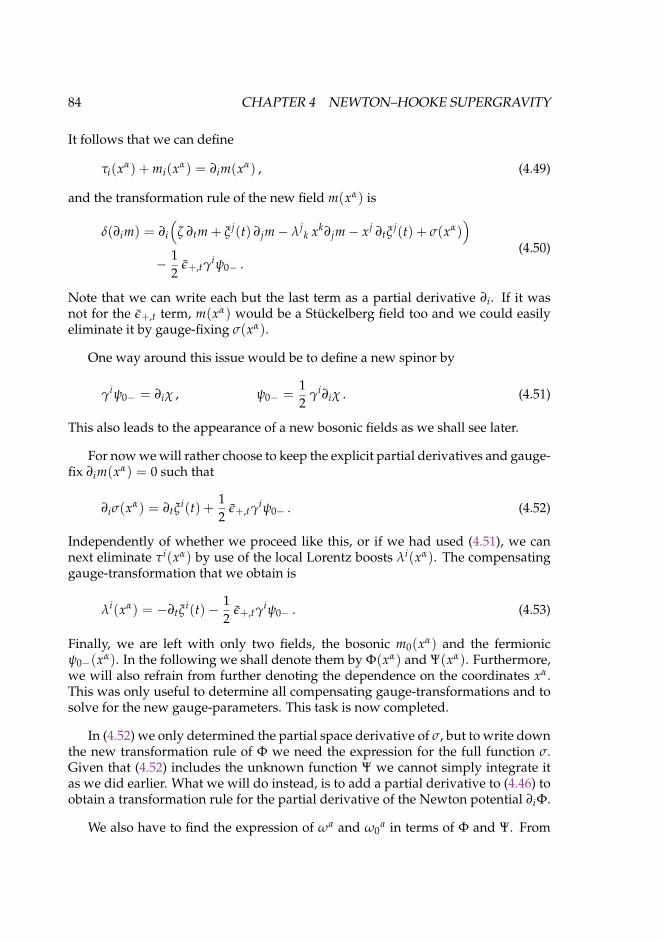
84 CHAPTER 4 NEWTON–HOOKE SUPERGRAVITY
It follows that we can define
τi(xα) + mi(xα) = ∂im(xα) , (4.49)
and the transformation rule of the new field m(xα) is
δ(∂im) = ∂i
(ζ ∂tm + ξ j(t) ∂jm− λj
k xk∂jm− xj ∂tξj(t) + σ(xα)
)− 1
2ε+,tγ
iψ0− .(4.50)
Note that we can write each but the last term as a partial derivative ∂i. If it wasnot for the ε+,t term, m(xα) would be a Stuckelberg field too and we could easilyeliminate it by gauge-fixing σ(xα).
One way around this issue would be to define a new spinor by
γiψ0− = ∂iχ , ψ0− =12
γi∂iχ . (4.51)
This also leads to the appearance of a new bosonic fields as we shall see later.
For now we will rather choose to keep the explicit partial derivatives and gauge-fix ∂im(xα) = 0 such that
∂iσ(xα) = ∂tξi(t) +
12
ε+,tγiψ0− . (4.52)
Independently of whether we proceed like this, or if we had used (4.51), we cannext eliminate τi(xα) by use of the local Lorentz boosts λi(xα). The compensatinggauge-transformation that we obtain is
λi(xα) = −∂tξi(t)− 1
2ε+,tγ
iψ0− . (4.53)
Finally, we are left with only two fields, the bosonic m0(xα) and the fermionicψ0−(xα). In the following we shall denote them by Φ(xα) and Ψ(xα). Furthermore,we will also refrain from further denoting the dependence on the coordinates xα.This was only useful to determine all compensating gauge-transformations and tosolve for the new gauge-parameters. This task is now completed.
In (4.52) we only determined the partial space derivative of σ, but to write downthe new transformation rule of Φ we need the expression for the full function σ.Given that (4.52) includes the unknown function Ψ we cannot simply integrate itas we did earlier. What we will do instead, is to add a partial derivative to (4.46) toobtain a transformation rule for the partial derivative of the Newton potential ∂iΦ.
We also have to find the expression of ωa and ω0a in terms of Φ and Ψ. From
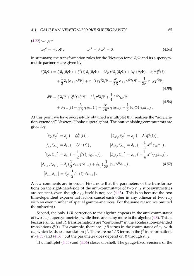
4.3 GALILEAN NEWTON–HOOKE SUPERGRAVITY 85
(4.22) we get
ω0a = −∂aΦ , ωi
a = ∂iωa = 0 . (4.54)
In summary, the transformation rules for the ’Newton force’ ∂iΦ and its supersym-metric partner Ψ are given by
δ(∂iΦ) = ζ ∂t(∂iΦ) + ξ j(t) ∂j(∂iΦ)− λjk xk∂j(∂iΦ) + λi
j (∂jΦ) + ∂t∂tξi(t)
+12
∂t(ε+,tγ
iΨ)+ ε−(t)γ0∂iΨ−
xj
2Rε+,tγ
j0∂iΨ−1
2Rε+,tγ
i0Ψ ,
(4.55)
δΨ = ζ ∂tΨ + ξ i(t) ∂iΨ− λij xj∂iΨ +
14
λabγabΨ
+ ∂tε−(t)−3
2Rγ0ε−(t) +
xi
2R2 γi0ε+,t −12(∂iΦ) γi0ε+,t .
(4.56)
At this point we have successfully obtained a multiplet that realizes the “accelera-tion-extended” Newton–Hooke superalgebra. The non-vanishing commutators aregiven by[
δζ , δξ i]= δξ i
(− ζξ i(t)
),
[δλi
j, δξ i]= δξ i
(− λi
jξj(t))
,[δζ , δε−
]= δε−
(− ζε−(t)
),
[δλi
j, δε−
]= δε−
(− 1
4λabγabε−
),[
δξ i , δε+
]= δε−
(− 1
2ξ i(t)γi0ε+,t
),
[δλi
j, δε+
]= δε+
(− 1
4λabγabε+,t
),[
δε1+ , δε2+
]= δζ
(12
ε2+γ0ε1+)+ δλi
j
( 12R
ε2+γijε1+)
, (4.57)[δε+ , δε−
]= δξ i
(12
ε−(t)γiε+,t)
.
A few comments are in order. First, note that the parameters of the transforma-tions on the right-hand-side of the anti-commutator of two ε+,t supersymmetriesare constant, even though ε+,t itself is not, see (4.43). This is so because the twotime-dependent exponential factors cancel each other in any bilinear of two ε+,twith an even number of spatial gamma-matrices. For the same reason we omittedthe subscript t.
Second, the only 1/R correction to the algebra appears in the anti-commutatorof two ε+,t supersymmetries, while there are many more in the algebra (4.8). This isbecause all Ga and Pa transformations are “combined” in the acceleration-extendedtranslations ξ i(t). For example, there are 1/R terms in the commutator of ε+ withε−, which leads to a translation ξ i. There are no 1/R terms in the ξ i transformationsin (4.55) and (4.56), but the parameter does depend on R through ε+,t.
The multiplet (4.55) and (4.56) closes on-shell. The gauge-fixed versions of the
86 CHAPTER 4 NEWTON–HOOKE SUPERGRAVITY
equations of motion (4.31) are
∂i∂iΦ =2
R2 , γi∂iΨ = 0 . (4.58)
One can readily check that they transform into each other under a supersymmetrytransformation.
Let us now come back to the idea put forward in (4.51). Our aim now is to derivethe transformation rule, such as (4.55), for the Newton potential only, not its spatialderivative. We thus introduce the new fermionic potential χ by
γiΨ = ∂iχ , Ψ =12
γi∂iχ . (4.59)
Then we can immediately write down the transformation rule for Φ:
δΦ = ζ ∂tΦ + ξ j(t) ∂jΦ + xi∂t∂tξi(t)− λj
k xk∂jΦ + σ(t)
+12
ε−(t)γ0i∂iχ +12
∂t(ε+,tχ
)+
xi
2Rε+,tγ
0∂iχ .(4.60)
We have to allow for an arbitrary time-dependent shift because we only know thetransformation of ∂iΦ. Equivalently, we see from (4.52) that such a shift is allowedin the compensating transformation.
To obtain the same result for χ is more challenging as we have to write (4.56), oractually γiδΨ, as a partial derivative acting on δχ. The problem here lies with theε+,t terms. We can write them as( xj
2R2 −12
∂jΦ)
γiγj0ε+,t =( xi
2R2 −12
∂iΦ)
γ0ε+,t −( xj
2R2 −12
∂jΦ)
εij ε+,t ,
(4.61)
where we use εij = γij0. Now we define a “dual Newton potential” Ξ by
∂iΦ−xi
R2 = −εij∂jΞ , ∂iΞ = εij
(∂jΦ−
xj
R2
). (4.62)
We thus get
δχ = ζ ∂tχ + ξ i(t) ∂iχ− λij xj∂iχ +
14
λabγabχ + xiγi ε−(t)
− 3xi
2Rγi0ε−(t)−
12
(Φ− xixi
2R2
)γ0ε+,t +
12
Ξ ε+,t + η(t) .(4.63)
It remains to derive the transformation rule for Ξ. From the variation of (4.62) we
4.4 CONNECTION TO THE NON-RELATIVISTIC LIMIT 87
note that
εij∂j(δΦ) = ∂i(δΞ) . (4.64)
This leads to
δΞ = ζ ∂tΞ + ξ j(t) ∂jΞ + εij xi∂t∂tξj(t) + εij
xiξ j(t)R2 − λj
k xk∂jΞ + σ(t)
+12
ε−(t)γi∂iχ +12
∂t(ε+,tγ
0χ)− xi
2Rε+,t∂iχ .
(4.65)
Using the defining equations (4.62), we can show that the multiplet given by (4.60),(4.63) and (4.65) also satisfies (4.57). In addition, we find more commutators givenby the time-dependent shift functions σ(t) and η(t) (and σ(t)). They lead to therelations[
δζ , δσ
]= δσ
(− ζσ(t)
),
[δξ i
1, δξ i
2
]= δσ
(ξ i
1(t)ξi2(t)− ξ i
2(t)ξi1(t)
),[
δζ , δη
]= δη
(− ζη(t)
),
[δξ i , δε−
]= δη
(− ξ i(t)γi ε−(t)
),[
δσ, δε+
]= δη
(12
σ(t)γ0ε+,t)
,[δλi
j, δη
]= δη
(− 1
4λabγabη(t)
),
(4.66)
which form an ideal of the acceleration-extended Newton–Hooke superalgebra.In this section we have derived a gauge-fixed version of Newton–Hooke su-
pergravity that is very much like the Galilean supergravity theory found in [77].Indeed, in the limit R → ∞ we recover the same results. Slight modifications areneeded in the gauge-fixing due to the additional 1/R contributions, such as thenew fixed time-dependence of ε+,t.
Let us remark here that it would be possible to define new spinors Ψ and χ thatdiffer from to the old ones only by an exponential factor exp(−tγ0/2R). This waywe could also make ε+ time-independent.
Note also that the Φ that we use here differs from the one used in [111]. There,we preferred to define the Newton potential such that its Laplacian is zero, ratherthan proportional to the cosmological constant, see (4.58). We will comment furtheron this in the conclusion section.
4.4 Connection to the non-relativistic limitThere are different ways to understand the results of section 4.2 as a non-relativisticlimit of anti-de Sitter supergravity. In particular, we can start from an on-shellanti-de Sitter supergravity multiplet to derive the transformation rules given in4.2, which is what we are going to do in this section. The other option wouldbe to use the off-shell Newton–Cartan multiplet of chapter 3. In the latter case,we would simply get the on-shell multiplet derived here by choosing the correct
88 CHAPTER 4 NEWTON–HOOKE SUPERGRAVITY
values for the auxiliary field S. While we set S = 0 to obtain on-shell Newton–Cartan supergravity we get the formulas of on-shell Newton–Hooke supergravityby using
S =1
2R, (4.67)
in the off-shell Newton–Cartan supergravity multiplet (3.78) and (3.79).In the following we shall briefly go through the first option, i.e. we take the
limit of on-shell N = (2, 0) anti-de Sitter supergravity [112]. The reason why weuse N = (2, 0) instead of N = (1, 1) was mentioned at several points previously.The corresponding multiplet is given by the cosmological extension of the N = 2theory of section 2.8, which consists of the transformation rules
δEµA =
12
δij ηi γAΨµj ,
δΨµi = Dµηi + εij ηj Vµ −1
2Rγµ ηi ,
δVµ = − 12R
εij ηiΨµj ,
(4.68)
and the equations of motion for the supergravity fields EµA, Ψµi and Vµ are given
by
Ψµνi = 0 , Vµν = 0 . (4.69)
The spin-connection ΩµAB(E, Ψi) is determined by the torsion constraint (2.85) and
it is given by (2.84). The multiplet (4.68) realizes the N = (2, 0) anti-de Sitter su-peralgebra (4.6).
Recall that in order to take the non-relativistic limit in section 3.4, we had toadd the gauge-field Mµ of the central charge generator Z of the N = 2 Poincaresuperalgebra. Its transformation rule was given in (3.51) and in order not to upsetthe counting of degrees of freedom we had to set its curvature to zero, eq. (3.52).Here, we need not add any such field as the gauge-field of R-symmetry Vµ willtake over that role. This can be inferred from looking at the contractions (3.2), (3.49)and (4.7) that lead to the N = (2, 0) Newton–Hooke superalgebra. Indeed, this isnot too surprising as in the limit where the cosmological constant goes to zero, theR-symmetry generator of the anti-de Sitter algebra becomes the central element ofthe Poincare superalgebra.
Before we apply the limiting procedure by using the contractions (3.2), (3.49)and (4.7), to decompose the relativistic gauge-fields in terms of non-relativisticones, we shall find it convenient (and necessary) to make one more redefinition.When we compare the transformation rule of the gauge-field Vµ, and the Vµ termsin the transformation rule of the gravitini, to the structure constants of the N =(2, 0) anti-de Sitter superalgebra (4.6), we note that there are additional factors of
4.4 CONNECTION TO THE NON-RELATIVISTIC LIMIT 89
R. In fact, Vµ is not exactly the gauge-field related to the generator R, but R timesVµ is. Therefore, we define
Mµ = −R Vµ . (4.70)
In the limit R → ∞ we go to Poincare supergravity and Mµ becomes Mµ. Theequation of motion Vµν = 0 then becomes equivalent to (3.52).
After the redefinition (4.70) the multiplet (4.68) goes to
δEµA =
12
δij ηi γAΨµj ,
δΨµi = Dµηi −1R
εij ηj Mµ −1
2Rγµ ηi ,
δMµ =12
εij ηiΨµj .
(4.71)
We take the non-relativistic limit in these transformation rules by using (3.3), (3.54)with the rescalings (3.55), along with
Mµ = ω τµ −1
2ωmµ , (4.72)
which follows from (4.7), and R → ω R. Since the transformation rules of thebosonic fields are identical to those of on-shell Poincare supergravity, see eqs. (2.80)and (3.51), we immediately derive the correct transformation rules for τµ, eµ
a andmµ given in (4.12). The correct transformation rules for the fermions, eq. (4.13), alsofollow from directly from (4.71). The expressions for the supercovariant curvatures(4.14) are derived from the torsion constraint (2.85) and the relativistic gravitinocurvature
Ψµνi = 2 ∂[µΨν]i −12
Ω[µABγABΨν]i −
2R
εij Ψ[µ Mν] +1R
γ[µΨν]i . (4.73)
The curvature of the relativistic spin-connection RµνAB(M) splits into the curvature
of the boost-connection Rµνa(G) and the non-relativistic spin-connection Rµν
ab(J).The derivation of the constraints also follows the analysis of section 3.4. We find(3.66), i.e. (4.16), and from consistency of the commutator algebra we deduce (4.26)and (4.27).
At this point we have derived all transformation rules, constraints and equa-tions of motion of the on-shell Newton–Hooke supergravity theory of section 4.2.There, we used gauging techniques to obtain the result, while here we started fromthe relativistic one. Therefore, we have shown that the non-relativistic limiting pro-cedure and gauging techniques indeed lead to the same result.
90 CHAPTER 4 NEWTON–HOOKE SUPERGRAVITY
4.5 SummaryIn this chapter we derived a new non-relativistic three-dimensional supergravitytheory. In particular, we considered a cosmological extension of “flat” Newton–Cartan supergravity. Our analysis also served as a check for the non-relativisticlimiting procedure that was developed in the last chapter.
Since this cosmological extension must reduce to the “flat” case, in the limitwhere the cosmological constant vanishes, i.e. for R → ∞, we expected to findresults that are similar to Newton–Cartan supergravity, that are only modified withorder 1/R corrections.
As it turns out the gauging procedure can indeed be done in much the sameway as Newton–Cartan supergravity was found in [77]. We also find the sameconstraint structure. The order 1/R correction with respect to the result of [77] canbe seen in the transformation rules only, but not explicitely in the constraints.
The Newton–Hooke supergravity background of section 4.2, as well as the Ga-lilean version of section 4.3, were used in [111] to consider a non-relativistic super-particle in such curved backgrounds. As noted earlier we use a slightly differentdefinition of the central charge gauge-field mµ and the Newton potential Φ in theGalilean version. If we denote the central charge gauge-field that was used in [111]by mµ we have
mµ = mµ + τµ(xρeρ
a)2
2 R2 . (4.74)
The reason for this choice was that the equation of motion for the Newton potentialφ is given by ∂i∂iφ = 0 rather than ∂i∂iΦ = 1/R2.
There are several possible extensions to the analysis of this chapter. First, in-spired by our work in the previous chapter one could try to find an off-shell for-mulation of three-dimensional Newton–Hooke supergravity. Since, Rµν
ab(J) = 0for S = 0, see e.g. the off-shell formulations of chapter 3, this might be equiv-alent to seeking an extension with Rµν
ab(J) 6= 0. Using the limiting procedure,this should be a fairly straightforward exercise. One could also try to extend thetheory by adding more supercharges and consider non-relativistic extended super-symmetry. Another interesting possibility would be to look for a formulation ofNewton–Hooke (super)gravity where we do not set the curvature Rµν(H) to zero.This would be equivalent to asking if there exists a torsion-full version of this the-ory. For this purpose it might of course be better to first consider only the bosoniccase.
5Schrodinger supergravity
This chapter discusses a “conformal” extension of Newton–Cartan supergrav-ity. The Schrodinger supergravity theory is obtained by gauging a Schrodingersuperalgebra. This construction of a Schrodinger supergravity theory is inter-esting in its own right as a non-relativistic version of “conformal” supergrav-ity, but it is also very useful as the basic building block for the non-relativisticversion of the conformal tensor calculus of the next chapter.
92 CHAPTER 5 SCHRODINGER SUPERGRAVITY
In this chapter we take a step towards “completing” the realm of three-dimensionalnon-relativistic supergravity theories. So far, we managed to find examples of Poin-care, i.e. Newton–Cartan, and anti-de Sitter, i.e. Newton–Hooke, supergravity. Onemissing piece is a theory of supergravity with more symmetries such as e.g. di-latations. To derive such a theory is the main objective of this chapter. Anothermotivation is that we are going to need this theory as a basis for the analysis thatwill follow in the next chapter 6.
We will derive this non-relativistic “superconformal” theory by gauging a su-peralgebra that is a “conformal” extension of the supergravity theories that we sawin chapters 3 and 4 [137]. We refer to this supergravity theory as Schrodinger super-gravity rather than conformal supergravity because we prefer to reserve the namenon-relativistic “conformal” supergravity multiplet for the multiplet that realizesthe gauging of the Galilean Conformal superalgebra, see [138–140]. The reason forthis is that the Schrodinger superalgebra, with only a single special conformal gen-erator, allows a mass parameter while the Galilean Conformal superalgebra doesnot. A related issue is that the Schrodinger algebra allows for the same central ex-tension with the symmetry generator Z as the Bargmann algebra. This is importantfor gauging too, as it allows to solve for the dependent gauge-fields in the sameway as when gauging the Bargmann algebra.
Note also that the algebra that we will use here, unlike the Galilean Conformalsuperalgebra mentioned before, is not obtained by contracting a relativistic one,hence we cannot employ the limiting procedure. But there is no need for that asmost of what we need was already found in [29]. Indeed, this reference treats thebosonic case of the analysis that we are about to perform here, i.e. a gauging of theSchrodinger algebra along the lines of chapters 2 and 4. For us, it only remains todiscuss the differences when we add fermionic generators.
In this section we thus discuss the gauging of a Schrodinger superalgebra. Thisis done in several steps. First, in section 5.1 we give the algebra. Then, in section5.2 we go through the gauging procedure. The transformation rules of all indepen-dent fields, the constraint structure and the expressions of the dependent fields interms of the independent ones is found in subsections 5.2.1–5.2.3. The full set ofcurvature constraints is discussed in detail in subsection 5.2.2. After calculating theexpressions of the dependent gauge fields in terms of independent ones in subsec-tion 5.2.3 we re-evaluate the transformation rules of the dependent fields to checkwhether or not they still coincide with those given by the algebra. Finally, havingdetermined the transformations of all fields we need to check if the set of curvatureconstraints that we imposed is a consistent one. In order to shorten our presenta-tion we moved this last point to subsection 5.2.2 too, even though it is in fact oneof the last steps of the analysis and can be performed only after having determinedthe transformations of the fields in 5.2.3. Finally, we conclude in section 5.3.
5.1 A SCHRODINGER SUPERALGEBRA 93
5.1 A Schrodinger superalgebra
The non-relativistic algebra that we are interested in is a supersymmetric extensionof the Schrodinger algebra [82, 83]. The Schrodinger algebra is the symmetry alge-bra of the Schrodinger equation and its rigid version also leaves the point-particleaction invariant. Supersymmetric extensions were first found in [89] as the sym-metry group of a spinning particle. However, this leads to an algebra with a Grass-mann valued vector charge, instead of a spinor (Q− in our notation). Because weare mainly interested in extensions of the Bargmann superalgebra with two spino-rial supercharges, see (3.50), we prefer if our Schrodinger algebra also contains suchoperators. Only then it is guaranteed that omitting the extra conformal symmetriesallows us to retrieve the Newton–Cartan supergravity theories that we dealt withpreviously. This is of particular importance for our analysis in the following chap-ter.
For the purpose of this work we restrict ourselves to using the z = 2 Schrodingeralgebra. This algebra, as well as its supersymmetric extension, is similar to theBargmann algebra in that it allows for the same central extension in the commutatorof spatial translations and Galilean boosts. This is important because it enables usto solve for the non-relativistic spin- and Galilean boost-connections and thus thegauging works in the same way as e.g. in [29, 77, 80].
As we choose to work in three space-time dimensions our preferred choice shallbe the algebra of [91]. For completeness let us mention that a more systematicstudy to find supersymmetric extensions of the Schrodinger algebra was carriedout in [92], where the same Schrodinger superalgebra was found. Furthermore, thealgebra that we are going to use also appeared in [141].
The most prominent difference with respect to the purely bosonic analysis in[29] is the existence (and necessity) of an extra bosonic symmetry generator that wedenote by R. This leads to the addition of an extra bosonic gauge-field rµ, a U(1)gauge-field in our case, with respect to their analysis. As we shall show in chapter6 this vector is related to the relativistic gauge-field of R-symmetry. Indeed, we willshow later an exact relation between the field rµ introduced here and the vector thatresults from taking the non-relativistic limit of the gauge-field of R-symmetry, Vµ,in the new minimal Poincare multiplet, see section 3.5.
To be concrete, we use the following set of commutators. The bosonic commu-tation relations of the Bargmann algebra, which we repeat here for convenience,[
Pa, Jbc]= 2 δa[b Pc] ,
[H, Ga
]= Pa ,[
Ga, Jbc]= 2 δa[b Gc] ,
[Pa, Gb
]= δab Z ,
(5.1)
are supplemented by the action of the dilatation operator D and special conformal
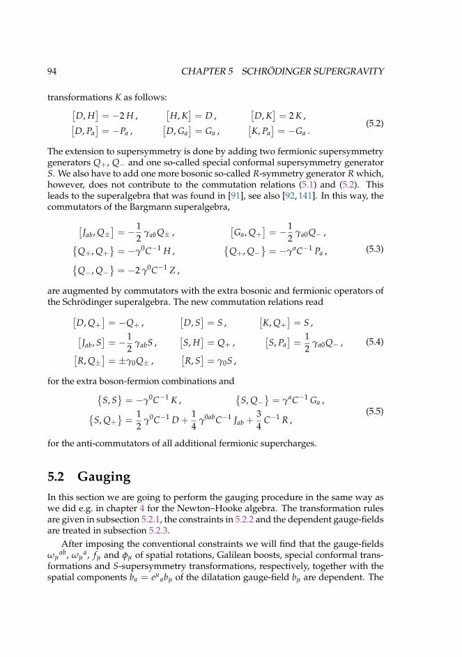
94 CHAPTER 5 SCHRODINGER SUPERGRAVITY
transformations K as follows:[D, H
]= −2 H ,
[H, K
]= D ,
[D, K
]= 2 K ,[
D, Pa]= −Pa ,
[D, Ga
]= Ga ,
[K, Pa
]= −Ga .
(5.2)
The extension to supersymmetry is done by adding two fermionic supersymmetrygenerators Q+, Q− and one so-called special conformal supersymmetry generatorS. We also have to add one more bosonic so-called R-symmetry generator R which,however, does not contribute to the commutation relations (5.1) and (5.2). Thisleads to the superalgebra that was found in [91], see also [92, 141]. In this way, thecommutators of the Bargmann superalgebra,
[Jab, Q±
]= −1
2γabQ± ,
[Ga, Q+
]= −1
2γa0Q− ,
Q+, Q+= −γ0C−1 H ,
Q+, Q−
= −γaC−1 Pa ,
Q−, Q−= −2 γ0C−1 Z ,
(5.3)
are augmented by commutators with the extra bosonic and fermionic operators ofthe Schrodinger superalgebra. The new commutation relations read[
D, Q+]= −Q+ ,
[D, S
]= S ,
[K, Q+
]= S ,[
Jab, S]= −1
2γabS ,
[S, H
]= Q+ ,
[S, Pa
]=
12
γa0Q− ,[R, Q±
]= ±γ0Q± ,
[R, S
]= γ0S ,
(5.4)
for the extra boson-fermion combinations andS, S= −γ0C−1 K ,
S, Q−
= γaC−1 Ga ,
S, Q+=
12
γ0C−1 D +14
γ0abC−1 Jab +34
C−1 R ,(5.5)
for the anti-commutators of all additional fermionic supercharges.
5.2 GaugingIn this section we are going to perform the gauging procedure in the same way aswe did e.g. in chapter 4 for the Newton–Hooke algebra. The transformation rulesare given in subsection 5.2.1, the constraints in 5.2.2 and the dependent gauge-fieldsare treated in subsection 5.2.3.
After imposing the conventional constraints we will find that the gauge-fieldsωµ
ab, ωµa, fµ and φµ of spatial rotations, Galilean boosts, special conformal trans-
formations and S-supersymmetry transformations, respectively, together with thespatial components ba = eµ
abµ of the dilatation gauge-field bµ are dependent. The
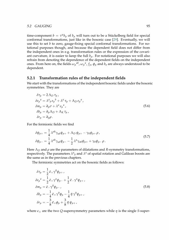
5.2 GAUGING 95
time-component b = τµbµ of bµ will turn out to be a Stuckelberg field for specialconformal transformations, just like in the bosonic case [29]. Eventually, we willuse this to set b to zero, gauge-fixing special conformal transformations. For no-tational purposes though, and because the dependent field does not differ fromthe independent ones in e.g. transformation rules or the expression of the covari-ant curvature, it is easier to keep the full bµ. For notational purposes we will alsorefrain from denoting the dependence of the dependent fields on the independentones. From here on, the fields ωµ
ab, ωµa, fµ, φµ and ba are always understood to be
dependent.
5.2.1 Transformation rules of the independent fieldsWe start with the transformations of the independent bosonic fields under the bosonicsymmetries. They are
δτµ = 2 ΛD τµ ,
δeµa = λa
b eµb + λa τµ + ΛD eµ
a ,
δmµ = ∂µσ + λa eµa ,
δbµ = ∂µΛD + ΛK τµ ,
δrµ = ∂µρ .
(5.6)
For the fermionic fields we find
δψµ+ =14
λabγabψµ+ + ΛD ψµ+ − γ0ψµ+ ρ ,
δψµ− =14
λabγabψµ− −12
λaγa0ψµ+ + γ0ψµ− ρ .(5.7)
Here ΛD and ρ are the parameters of dilatations and R-symmetry transformations,respectively. The parameters λa
b and λa of spatial rotation and Galilean boosts arethe same as in the previous chapters.
The fermionic symmetries act on the bosonic fields as follows:
δτµ =12
ε+γ0ψµ+ ,
δeµa =
12
ε+γaψµ− +12
ε−γaψµ+ ,
δmµ = ε−γ0ψµ− ,
δbµ = −14
ε+γ0φµ −14
η γ0ψµ+ ,
δrµ = −38
ε+φµ +38
η ψµ+ ,
(5.8)
where ε± are the two Q-supersymmetry parameters while η is the single S-super-
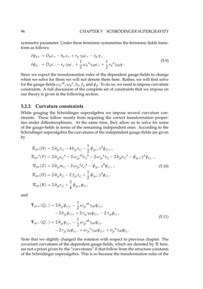
96 CHAPTER 5 SCHRODINGER SUPERGRAVITY
symmetry parameter. Under these fermionic symmetries the fermionic fields trans-form as follows:
δψµ+ = Dµε+ − bµ ε+ + rµ γ0ε+ − τµ η ,
δψµ− = Dµε− − rµ γ0ε− +12
ωµaγa0ε+ +
12
eµaγa0η .
(5.9)
Since we expect the transformation rules of the dependent gauge-fields to changewhen we solve for them we will not denote them here. Rather, we will first solvefor the gauge-fields ωµ
ab, ωµa, ba, fµ and φµ. To do so, we need to impose curvature
constraints. A full discussion of the complete set of constraints that we impose onour theory is given in the following section.
5.2.2 Curvature constraintsWhile gauging the Schrodinger superalgebra we impose several curvature con-straints. These follow mostly from requiring the correct transformation proper-ties under diffeomorphisms. At the same time, they allow us to solve for someof the gauge-fields in terms of the remaining independent ones. According to theSchrodinger superalgebra the curvatures of the independent gauge-fields are givenby
Rµν(H) = 2 ∂[µτν] − 4 b[µτν] −12
ψ[µ+γ0ψν]+ ,
Rµνa(P) = 2 ∂[µeν]
a − 2 ω[µabeν]
b − 2 ω[µaτν] − 2 b[µeν]
a − ψ[µ+γaψν]− ,
Rµν(Z) = 2 ∂[µmν] − 2 ω[µaeν]
a − ψ[µ−γ0ψν]− ,
Rµν(D) = 2 ∂[µbν] − 2 f[µτν] +12
ψ[µ+γ0φν] ,
Rµν(R) = 2 ∂[µrν] +34
ψ[µ+φν] ,
(5.10)
and
Ψµν+(Q+) = 2 ∂[µψν]+ −12
ω[µabγabψν]+
− 2 b[µψν]+ + 2 r[µγ0ψν]+ − 2 τ[µφν] ,
Ψµν−(Q−) = 2 ∂[µψν]− −12
ω[µabγabψν]−
− 2 r[µγ0ψν]− + ω[µaγa0ψν]+ + e[µ
aγa0φν] .
(5.11)
Note that we slightly changed the notation with respect to previous chapter. Thecovariant curvatures of the dependent gauge-fields, which are denoted by R here,are not a priori given by the “curvatures” R that follow from the structure constantsof the Schrodinger superalgebra. This is so because the transformation rules of the

5.2 GAUGING 97
dependent gauge-fields are not necessarily equal to the ones that follow from thestructure constants of the algebra, see e.g. the fermionic transformation rules givenin eqs. (5.37). For the following discussion we will need the curvatures of spatialrotations, Galilean boosts and S-supersymmetry. In the case of spatial rotations thefull curvature coincides with the expression that follows from the structure con-stants, i.e. R(J) = R(J), but in the other two cases there are additional terms in Rsince the fermionic transformation rules of those gauge-fields contain extra termsbeyond those that are determined by the structure constants, see eq. (5.37). Wetherefore have that
Rµνab(J) = 2 ∂[µων]
ab − 12
φ[µγ0abψν]+ , (5.12)
but that
Rµνa(G) = Rµν
a(G) + additional terms , (5.13)
with the structure constant dependent part Rµνa(G) given by
Rµνa(G) = 2 ∂[µων]
a − 2 ω[µabων]
b − 2 ω[µabν] − 2 f[µeν]
a + φ[µγaψν]− . (5.14)
We will not need the “additional terms” in R(G) except for a special trace combi-nation in which case the full expression forR(G) is given by
R0aa(G) = R0a
a(G)− eµa ψµ−γ0Ψa0−(Q−) . (5.15)
The additional terms in (5.13) were given explicitly in (3.69), using a different nota-tion though. Moving on with our new notation we find the curvature of the gauge-field of S-supersymmetry is given by
Rµν(S) = 2 ∂[µφν] −12
ω[µabγabφν] + 2 b[µ φν] + 2 r[µ γ0φν] + 2 f[µ ψν]+
+ 2 γ0ψ[µ+
[14
εabRν]0ab(J)−Rν]0(R)
]− 2 γcψ[µ−
[14
εabRν]cab(J) +Rν]c(R)
],
(5.16)
where only the first line comprises terms that follow from the structure constants.
In the following subsection we will solve for the gauge-fields ωµab, ωµ
a, ba, fµ
and φµ in terms of the independent ones using the following set of conventionalconstraints:
Rµνa(P) = 0 , Rµν(Z) = 0 , Ra0(H) = 0 ,
Ψa0+(Q+) = 0 , γaΨa0−(Q−) = 0 ,Ra0(D) = 0 , R0a
a(G) = 0 .
(5.17)
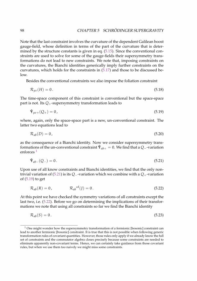
98 CHAPTER 5 SCHRODINGER SUPERGRAVITY
Note that the last constraint involves the curvature of the dependent Galilean boostgauge-field, whose definition in terms of the part of the curvature that is deter-mined by the structure constants is given in eq. (5.15). Since the conventional con-straints are used to solve for some of the gauge-fields their supersymmetry trans-formations do not lead to new constraints. We note that, imposing constraints onthe curvatures, the Bianchi identities generically imply further constraints on thecurvatures, which holds for the constraints in (5.17) and those to be discussed be-low.
Besides the conventional constraints we also impose the foliation constraint
Rµν(H) = 0 . (5.18)
The time-space component of this constraint is conventional but the space-spacepart is not. Its Q+-supersymmetry transformation leads to
Ψµν+(Q+) = 0 , (5.19)
where, again, only the space-space part is a new, un-conventional constraint. Thelatter two equations lead to
Rab(D) = 0 , (5.20)
as the consequence of a Bianchi identity. Now we consider supersymmetry trans-formations of the un-conventional constraint Ψab+ = 0. We find that a Q−-variationenforces 1
Ψab−(Q−) = 0 . (5.21)
Upon use of all know constraints and Bianchi identities, we find that the only non-trivial variation of (5.21) is its Q−-variation which we combine with a Q+-variationof (5.19) to get
Rab(R) = 0 , Rabcd(J) = 0 . (5.22)
At this point we have checked the symmetry variations of all constraints except thelast two, i.e. (5.22). Before we go on determining the implications of their transfor-mations we note that using all constraints so far we find the Bianchi identity
Rab(S) = 0 . (5.23)
1 One might wonder how the supersymmetry transformation of a fermionic [bosonic] constraint canlead to another fermionic [bosonic] constraint. It is true that this is not possible when following generictransformation rules of covariant quantities. However, those rules only apply if we already know the fullset of constraints and the commutator algebra closes precisely because some constraints are needed toeliminate apparently non-covariant terms. Hence, we can certainly take guidance from those covariantrules, but when we use them too naively we might miss some constraints.
5.2 GAUGING 99
This identity is useful in showing that the only non-trivial transformation of thefirst constraint in (5.22) leads to 1
34
εabRµνab(J) = Rµν(R) . (5.24)
Since (5.24) essentially identifiesR(J) withR(R) we have derived all consequencesof (5.22). The constraint (5.24) itself is inert under all symmetries and hence we havederived the full set of un-conventional constraints that follow from (5.18).
In summary, the set of constraints comprises the following chain of un-conven-tional constraints:
Rab(H) = 0Q+−→ Ψab+ = 0
Q−−→ Ψab− = 0 −→Ψab+ = 0Ψab− = 0
Q±−→ Rab(R) = 0
Q+−→ 34
εabRµνab(J) = Rµν(R) .
(5.25)
The most important Bianchi identities that feature in the discussion above are givenby
Rab(D) = 0 , R0[ab](G) = 0 ,
Rab(S) = 0 , Rabc(G) = 2R0[a
b]c(J) .(5.26)
The equations (5.17), (5.25) and (5.26) comprise all constraints of the Schrodingersupergravity theory.
5.2.3 The dependent gauge-fields
Let us now determine the expressions of the dependent gauge-fields. We first de-termine the spatial component of bµ. UsingRa0(H) = 0 we find
ba = eµabµ =
12
eµaτν
(2 ∂[µτν] −
12
ψ[µ+γ0ψν]+
). (5.27)
Like in the bosonic case [29], the (independent) scalar b = τµbµ is a Stuckelbergfield for special conformal transformations:
δb = ΛK + τµ∂µΛD − 2 ΛD b− λa ba −14
τµ (ε+γ0φµ + η γ0ψµ+)
− 12
b ε+γ0ψρ+τρ − 12
ba τρ (ε+γaψρ− + ε−γaψρ+) .(5.28)
100 CHAPTER 5 SCHRODINGER SUPERGRAVITY
Therefore, we could choose to set b = 0 already at this point. Doing so wouldinduce the compensating transformation
ΛK = −τµ∂µΛD + λa ba +14
τµ (ε+γ0φµ + η γ0ψµ+)
+12
ba τρ (ε+γaψρ− + ε−γaψρ+) .(5.29)
However, we will not set b = 0 just yet because we want to keep special conformaltransformations in our supergravity background. Still, we would also like to pointout that since no independent field transforms under special conformal transforma-tions there would in essence be no effect from this gauge-fixing, when consideringonly independent fields.
We proceed with determining the spin- and boost-connection ωµab and ωµ
a.This calculation works in precisely the same way as we described in chapter 4,using the constraintsRµν
a(P) = 0 andRµν(Z) = 0. It leads to the expressions
ωµab = 2 eν[a(∂[νeµ]
b] − 12
ψ[ν+γb]ψµ]− − b[ν eµ]b])
+ eµceρaeνb(∂[ρeν]
c − 12
ψ[ρ+γcψν]− − b[ρ eν]c)
− τµeρaeνb(∂[ρmν] −12
ψ[ρ−γ0ψν]−)
,
(5.30)
ωµa = −τν
(∂[νeµ]
a − 12
ψ[ν+γaψµ]− − b[ν eµ]a)
+ eµceρaτν
(∂[ρeν]
c − 12
ψ[ρ+γcψν]− − b[ρ eν]c)
+ eνa(∂[µmν] −12
ψ[µ−γ0ψν]−)− τµeρaτν
(∂[ρmν] −
12
ψ[ρ−γ0ψν]−)
,
(5.31)
which of course differ from (4.21) and (4.22) because of the additional dilatationgauge-field bµ. The field φµ is determined by the constraints in the third line of(5.17) giving
eµa φµ = −eµ
aτν(2 ∂[µψν]+ −
12
ω[µabγabψν]+ − 2 b[µψν]+ + 2 r[µγ0ψν]+
),
τµφµ = τµeνc γ0c (2 ∂[µψν]− −
12
ω[µabγabψν]− + ω[µ
aγa0ψν]+ − 2 r[µγ0ψν]−)
.
(5.32)

5.2 GAUGING 101
Thus, we obtain
φµ = −τν(2 ∂[µψν]+ −
12
ω[µabγabψν]+ − 2 b[µψν]+ + 2 r[µγ0ψν]+
)+ τµτρeν
cγ0c (2 ∂[ρψν]− −12
ω[ρabγabψν]− + ω[ρ
aγa0ψν]+ − 2 r[µγ0ψν]−)
.
(5.33)
Finally, to solve for fµ we use Ra0(D) = 0 and R0aa(G) = 0. We get, from the first
and the second identity, respectively,
eµa fµ = eµ
aτν(2 ∂[µbν] +
12
ψ[µ+γ0φν]
),
τµ fµ =12
τµeνa(2 ∂[µων]
a − 2 ω[µabων]
b − 2 ω[µabν] + φ[µγaψν]−
)− 1
2eµ
a ψµ−γ0ψa0− .
(5.34)
Hence, the full expression for fµ is
fµ = τν(2 ∂[µbν] +
12
ψ[µ+γ0φν]
)− 1
2τµeρ
a ψρ−γ0ψa0−
+12
τµτρeνa(2 ∂[ρων]
a − 2 ω[ρabων]
b − 2 ω[ρabν] + φ[ργaψν]−
).
(5.35)
At this point we have found all dependent gauge-fields in terms of the independentones. In the following we derive the transformation rules of the dependent fields.We find
δωµab = ∂µλab ,
δωµa = ∂µλa −ωµ
abλb + bµλa + λa
b ωµb −ΛD ωµ
a + ΛK eµa ,
δ fµ = ∂µΛK + 2 ΛK bµ − 2 ΛD fµ − τµ λbR0aab(J) ,
δφµ =14
λabγabφµ −ΛD φµ −ΛK ψµ+ − γ0φµ ρ ,
(5.36)
i.e. most transformation rules are un-altered. The only change appears for fµ, whichacquires a non-trivial transformation under Galilean boosts. In [29] this was cir-cumvented by redefining fµ by adding terms with mµ and Rµν
ab(J) in one of theconventional constraints that is used to solve for fµ. However, then the field ac-quired a non-trivial transformation under the central charge symmetry Z. We willnot attempt any redefinition of that kind here.
102 CHAPTER 5 SCHRODINGER SUPERGRAVITY
Concerning the fermionic Q and S-transformations we calculate
δωµab = −1
4ε+γab0φµ +
14
η γab0ψµ+ ,
δωµa = ε−γ0Ψµ
a− −
12
ε−γaφµ +14
eµb ε+γbΨa0−
+14
ε+γaΨµ0− −12
η γaψµ− ,
δφµ = Dµη + bµ η + rµ γ0η + fµ ε+ + γ0ε+[1
4εabRµ0
ab(J)−Rµ0(R)]
+ γcε−[1
4εabRµc
ab(J) +Rµc(R)]
.
(5.37)
These transformations allow us to explicitly check that the commutator algebra (ofthe fermionic symmetries) is realized by the formula[
δ(Q1, S1), δ(Q2, S2)]= δg.c.t.
(Ξµ)+ δJ
(Λab)+ δG
(Λa)+ δZ
(Σ)+ δR
(ρR)
+ δQ+
(Υ+)+ δQ−
(Υ−)+ δD
(λD)+ δK
(λK)
,(5.38)
where the parameters are given by
Ξµ =12
ε2+γ0ε1+ τµ +12(ε2+γaε1− + ε2−γaε1+
)eµ
a ,
Λab = −Ξµωµab +
14(ε1+γ0abη2 − η1 γ0abε2+
),
Λa = −Ξµωµa +
12(ε1−γaη2 + η1 γaε2−
),
Σ = −Ξµmµ + ε2−γ0ε1− ,
λD = −Ξµbµ +14(ε1+γ0η2 + η1 γ0ε2+
),
Υ± = −Ξµψµ± ,
λK = −Ξµ fµ +12
η2 γ0η1 ,
ρR = −Ξµrµ +38(ε1+η2 − η1 ε2+
),
η = −Ξµφµ .
(5.39)
This finishes the discussion of the “conformal” supergravity background.
Note that our analysis of the Schrodinger theory is not fully complete, since wedid not derive the variation of the dependent field fµ under fermionic symmetries.Even so, this was not needed to show that the set of constraints (5.25) is a consistentone and that the commutator algebra closes on all independent fields.
5.3 CONCLUDING REMARKS 103
5.3 Concluding remarksIn previous works, see [77] and also chapter 4, the gauging was followed by agauge-fixing to a Galilean observer. However, as shown in [29] this procedure doesnot lead to any new results with respect to the Bargmann case. The reason is thatthe Schrodinger theory is “gauge-equivalent” to the Newton–Cartan theory plusa scalar, see also [102]. Gauge-fixing the scalar, much in the same way as we aregoing to do in the next chapter, eliminates the dilatation symmetry and from thereon the theory is equivalent to Newton–Cartan gravity. Therefore, we refrain fromperforming this analysis here.
An interesting problem is to define dynamics for this supergravity background.It is indeed highly non-trivial to find an equation of motion for the independentfields that is invariant under all symmetries. In the case of Newton–Cartan (su-per)gravity we would interpret the constraint R0a
a(G) = 0 as the equation of mo-tion. Here, R0a
a(G) = 0 is a conventional constraint that we used to solve for fµ.Because this constraint is not invariant under boost transformations we cannot re-duce it to an invariant equation of motion. Not unless we require thatRµν
ab(J) = 0which, on the other hand, is not part of the constraints that we discussed in sub-section 5.2.2. A systematic approach to find an equation of motion for Schrodinger(super)gravity can be found in [102].
While it is interesting to derive a non-relativistic theory of “conformal” super-gravity, this was not the only motivation for us to do so. In the next chapter, wewill use the Schrodinger supergravity theory as the basis for the Schrodinger ten-sor calculus. For example, we will derive a theory of Newton–Cartan supergravitywith torsion. This is not surprising as e.g. the analysis in [29] proved that gaugingthe Schrodinger algebra can be used for precisely that purpose. In hindsight, theinteresting and surprising fact is that there indeed does exist a truncation to zerotorsion, i.e. to the Newton–Cartan supergravity theories that we have seen so far.
Last but not least, let us draw your attention to a connection of the theory dis-cussed in this chapter, to condensed matter theory. The authors of [73] used the verysame non-relativistic Chern–Simons theory of [91], whose algebra we just gaugedin this section, and showed that it too can be used to describe features of the frac-tional Quantum Hall effect.

104
6Schrodinger tensor calculus
In this chapter we present another generalization of three-dimensional Newton–Cartan supergravity, namely the theory with non-zero torsion. To derive it weuse “superconformal”, hereafter called Schrodinger, techniques where compen-sating matter multiplets are used to gauge-fix the extra symmetries (with re-spect to the Bargmann algebra) of the Schrodinger supergravity theory of thelast chapter.
106 CHAPTER 6 SCHRODINGER TENSOR CALCULUS
In this last chapter we derive yet another generalization of Newton–Cartan su-pergravity, the theory with non-zero torsion [137]. To do so, we will use a non-relativistic version of the superconformal tensor calculus, see e.g. [97] for an intro-duction and references. This chapter will also serve as an exposition of how thesemethods work and how they can be applied in the non-relativistic case.
Before doing this in the non-relativistic case we will briefly recall how it worksin the relativistic case. The main idea is to gauge-fix the extra symmetries thatthe superconformal theory possesses with respect to the Poincare symmetries. Forthis purpose, one adds (at least one) so-called compensator multiplet that also re-alizes the superconformal algebra. Then, one fixes dilatations and conformal S-supersymmetry by eliminating/gauge-fixing fields of the compensator multiplet.
Let us be more concrete and discuss a well-known example. The four-dimensio-nal N = 1 Weyl multiplet consists of the independent fields (Eµ
A, Ψµ, Aµ) whichrealize the superconformal algebra. (Special conformal symmetries were gauge-fixed by setting the gauge-field of dilatations Bµ to zero.) As a compensator, wemight consider the chiral multiplet which comprises two complex scalars and aspinor (Φ, χ, F). To derive a Poincare multiplet from the Weyl multiplet we needto gauge-fix dilatations D, R-symmetry and conformal S-supersymmetry. We maychoose
Φ = 1 : fixes dilatations D and R-symmetry ,χ = 0 : fixes conformal S-supersymmetry .
(6.1)
With this analysis we derive the old minimal Poincare multiplet which consists of(Eµ
A, Ψµ, Aµ, F) [142–145]. Alternatively, one can use a different compensator mul-tiplet to obtain the new minimal formulation with the fields (Eµ
A, Ψµ, Vµ, Aµ, D)[146–148]. Here D is a real scalar and the theory still enjoys a global U(1)-symmetry.
We will find that the non-relativistic case works quite similarly. Our equivalentof the Weyl multiplet is given by the Schrodinger multiplet which we derived inchapter 5 and it consists of the independent fields (τµ, eµ
a, mµ, rµ, ψµ±). In analogyto the relativistic case we eliminate the scalar b to get rid of special conformal trans-formations.1 Furthermore, we need to gauge-fix dilatations and S-supersymmetryusing a compensating matter multiplet.
In this chapter we will use two different multiplets for that purpose, which arerelated to the scalar and the vector multiplet, respectively, in the relativistic case.This will lead to the non-relativistic analogs of the old and the new minimal for-mulation of Poincare supergravity, which we discussed above. In particular, wefind the “old” minimal multiplet with the independent field content (see subsec-tion 6.2.1)
non-relativistic old minimal :(τµ, eµ
a, mµ, rµ, ψµ±, χ−, F1, F2)
, (6.2)
1 As shown in the (bosonic) analysis in [102] there is in fact no need to eliminate b as it simply dropsout of all expressions. We did not investigate if this is also true in the supersymmetric case.
6.1 MATTER COUPLINGS 107
and the “new” minimal formulation with (see subsection 6.2.2)
non-relativistic new minimal :(τµ, eµ
a, mµ, rµ, ψµ±, S)
. (6.3)
It was shown in [29], and chapter 5, that the gauging of the Schrodinger algebranaturally leads to Newton–Cartan geometry with torsion. In the previous chapterwe found that the torsion is provided by the spatial components of the dilatationgauge-field ba, that are dependent on the other fields. This feature remained inthe construction of the Schrodinger supergravity multiplet and our non-relativisticSchrodinger tensor calculus therefore naturally leads to torsionfull Newton–Cartansupergravity theories. In this way, we are thus able to extend the constructionsof [77] and chapter 3 to the torsionfull case. The torsionless case can be retrieved byputting the torsion to zero. As the torsion is provided by gauge-field componentsthat depend on the other fields in the supergravity multiplet, this truncation is non-trivial and its consistency has to be examined. We will study this truncation onlyin the case of non-relativistic new minimal supergravity and we will show that thistruncation leads to the off-shell three-dimensional N = 2 theory of chapter 3.
We have organized this chapter as follows. The next section 6.1 is entirely de-voted to the derivation of two non-relativistic matter multiplets. These will be usedin section 6.2 to derive Newton–Cartan supergravity with non-zero torsion. Thetruncation to a theory with zero torsion is investigated in section 6.3 and in section6.4 we end with a discussion.
6.1 Matter couplingsIn this section we present matter multiplets that realize the same commutators cor-responding to the Schrodinger superalgebra as we derived for the Schrodinger su-pergravity multiplet, see eq. (5.39). These multiplets will be used in the follow-ing section as compensator multiplets to derive off-shell formulations of Newton–Cartan supergravity.
One of those off-shell formulations was discussed in chapter 3. We obtainedit by taking a non-relativistic limit of the three-dimensional N = 2 new minimalPoincare multiplet [114]. Recall that the new minimal Poincare multiplet followsfrom superconformal techniques using a compensating (relativistic) vector multi-plet. Hence, in order to derive its non-relativistic analog, we should use as a com-pensator a non-relativistic vector multiplet. This is one of the two non-relativisticmatter multiplets which we derive in this section. The other one is the scalar mul-tiplet, which we shall later use to derive a new off-shell formulation of Newton–Cartan supergravity.
This section also focuses on the method that we use to derive those novel mat-ter multiplets. It would be very efficient if we could use the non-relativistic lim-iting procedure of chapter 3. However, we cannot do so because the Schrodingersuperalgebra does not follow from the contraction of any relativistic algebra andthe same applies to the Schrodinger supergravity theory. Instead, we shall pro-
108 CHAPTER 6 SCHRODINGER TENSOR CALCULUS
ceed in the following way. We start from the rigid version of a relativistic mattermultiplet that realizes the Poincare superalgebra and take the non-relativistic limitthereof.2 The important thing is that at this point we have derived the field contentof the non-relativistic multiplet. It turns out that the same multiplet also providesa representation of the rigid Schrodinger superalgebra. Therefore, once we haveobtained this non-relativistic matter multiplet, we can couple it to the fields of theSchrodinger supergravity theory, thereby realizing the commutator algebra derivedin the previous section, in the standard way.
6.1.1 The scalar multipletIn this subsection we construct the non-relativistic scalar multiplet. We start withthe three-dimensional rigid relativistic N = 2 scalar multiplet which comprisestwo complex scalar and two spinors. In real notation we are thus left with thefields (ϕ1, ϕ2, χ1, χ2; F1, F2):
δϕ1 = η1χ1 + η2χ2 ,δϕ2 = η1χ2 − η2χ1 ,
δχ1 =14
γµ∂µ ϕ1 η1 −14
γµ∂µ ϕ2 η2 −14
F1 η1 −14
F2 η2 ,
δχ2 =14
γµ∂µ ϕ2 η1 +14
γµ∂µ ϕ1 η2 −14
F2 η1 +14
F1 η2 ,
δF1 = −η1γµ∂µχ1 + η2γµ∂µχ2 ,
δF2 = −η1γµ∂µχ2 − η2γµ∂µχ1 .
(6.4)
Note that we do not consider bosonic transformations yet. We will add them onlyto the final result.
Let us recall the salient points of the limiting procedure that we introduced inchapter 3. To take the limit we use a limiting parameter ω which we will send toinfinity. The rescaling of the symmetry parameters follows from the Inonu–Wignercontraction of the related symmetry generators. This means for example that wewill require
ε± =ω∓1/2√
2(η1 ± γ0η2) . (6.5)
It remains to find the scalings of all other fields which are not determined a priori bythe procedure, like for example the scalings of the auxiliary fields. Those scalingsare relatively easy to find and it turns out that we need to use
χ± =ω−1±1/2√
2(χ1 ± γ0χ2) , (6.6)
2 This (rigid) limit coincides with the non-relativistic limit performed in [65].
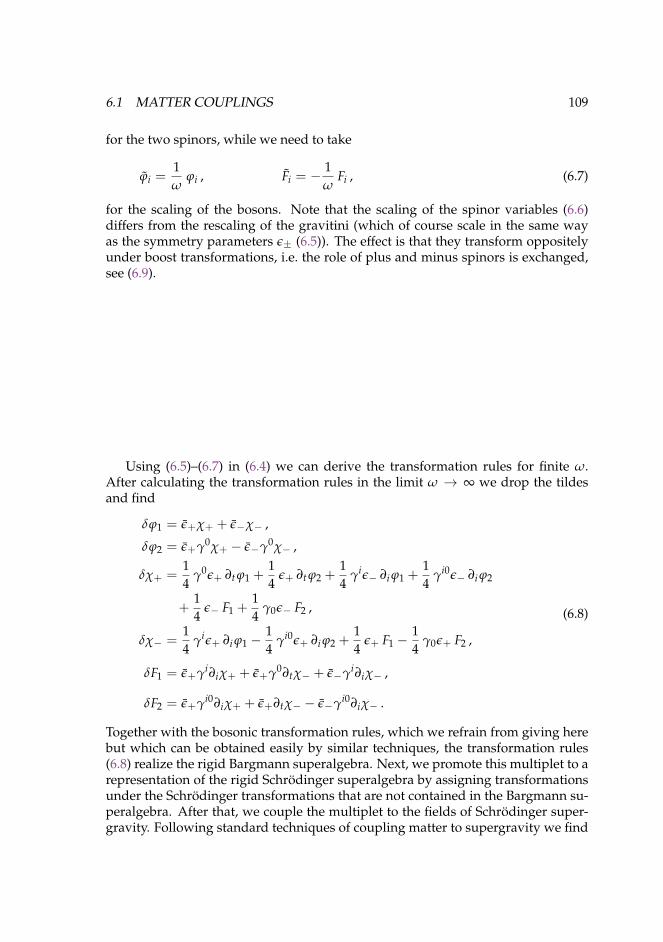
6.1 MATTER COUPLINGS 109
for the two spinors, while we need to take
ϕi =1ω
ϕi , Fi = −1ω
Fi , (6.7)
for the scaling of the bosons. Note that the scaling of the spinor variables (6.6)differs from the rescaling of the gravitini (which of course scale in the same wayas the symmetry parameters ε± (6.5)). The effect is that they transform oppositelyunder boost transformations, i.e. the role of plus and minus spinors is exchanged,see (6.9).
Using (6.5)–(6.7) in (6.4) we can derive the transformation rules for finite ω.After calculating the transformation rules in the limit ω → ∞ we drop the tildesand find
δϕ1 = ε+χ+ + ε−χ− ,
δϕ2 = ε+γ0χ+ − ε−γ0χ− ,
δχ+ =14
γ0ε+ ∂t ϕ1 +14
ε+ ∂t ϕ2 +14
γiε− ∂i ϕ1 +14
γi0ε− ∂i ϕ2
+14
ε− F1 +14
γ0ε− F2 ,
δχ− =14
γiε+ ∂i ϕ1 −14
γi0ε+ ∂i ϕ2 +14
ε+ F1 −14
γ0ε+ F2 ,
δF1 = ε+γi∂iχ+ + ε+γ0∂tχ− + ε−γi∂iχ− ,
δF2 = ε+γi0∂iχ+ + ε+∂tχ− − ε−γi0∂iχ− .
(6.8)
Together with the bosonic transformation rules, which we refrain from giving herebut which can be obtained easily by similar techniques, the transformation rules(6.8) realize the rigid Bargmann superalgebra. Next, we promote this multiplet to arepresentation of the rigid Schrodinger superalgebra by assigning transformationsunder the Schrodinger transformations that are not contained in the Bargmann su-peralgebra. After that, we couple the multiplet to the fields of Schrodinger super-gravity. Following standard techniques of coupling matter to supergravity we find
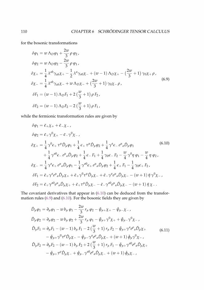
110 CHAPTER 6 SCHRODINGER TENSOR CALCULUS
for the bosonic transformations
δϕ1 = w ΛD ϕ1 +2w3
ρ ϕ2 ,
δϕ2 = w ΛD ϕ2 −2w3
ρ ϕ1 ,
δχ+ =14
λabγabχ+ −12
λaγa0χ− + (w− 1)ΛDχ+ −(2w
3+ 1)
γ0χ+ ρ ,
δχ− =14
λabγabχ− + w ΛDχ− +(2w
3+ 1)
γ0χ− ρ ,
δF1 = (w− 1)ΛDF1 + 2(w
3+ 1)
ρ F2 ,
δF2 = (w− 1)ΛDF2 − 2(w
3+ 1)
ρ F1 ,
(6.9)
while the fermionic transformation rules are given by
δϕ1 = ε+χ+ + ε−χ− ,
δϕ2 = ε+γ0χ+ − ε−γ0χ− ,
δχ+ =14
γ0ε+ τµDµ ϕ1 +14
ε+ τµDµ ϕ2 +14
γaε− eµaDµ ϕ1
+14
γa0ε− eµaDµ ϕ2 +
14
ε− F1 +14
γ0ε− F2 −w4
γ0η ϕ1 −w4
η ϕ2 ,
δχ− =14
γaε+ eµaDµ ϕ1 −
14
γa0ε+ eµaDµ ϕ2 +
14
ε+ F1 −14
γ0ε+ F2 ,
δF1 = ε+γaeµaDµχ+ + ε+γ0τµDµχ− + ε−γaeµ
aDµχ− − (w + 1) η γ0χ− ,
δF2 = ε+γa0eµaDµχ+ + ε+τµDµχ− − ε−γa0eµ
aDµχ− − (w + 1) η χ− .
(6.10)
The covariant derivatives that appear in (6.10) can be deduced from the transfor-mation rules (6.9) and (6.10). For the bosonic fields they are given by
Dµ ϕ1 = ∂µ ϕ1 − w bµ ϕ1 −2w3
rµ ϕ2 − ψµ+χ+ − ψµ−χ− ,
Dµ ϕ2 = ∂µ ϕ2 − w bµ ϕ2 +2w3
rµ ϕ1 − ψµ+γ0χ+ + ψµ−γ0χ− ,
DµF1 = ∂µF1 − (w− 1) bµ F1 − 2(w
3+ 1)
rµ F2 − ψµ+γaeρaDρχ+
− ψµ+γ0τρDρχ− − ψµ−γaeρaDρχ− + (w + 1) φµγ0χ− ,
DµF2 = ∂µF2 − (w− 1) bµ F2 + 2(w
3+ 1)
rµ F1 − ψµ+γa0eρaDρχ+
− ψµ+τρDρχ− + ψµ−γa0eρaDρχ− + (w + 1) φµχ− ,
(6.11)

6.1 MATTER COUPLINGS 111
while for the covariant derivatives of the fermions we find
Dµχ+ = Dµχ+ +12
ωµaγa0χ− − (w− 1) bµχ+ +
(2w3
+ 1)
rµ γ0χ+
− 14
γ0ψµ+ τρDρ ϕ1 −14
ψµ+ τρDρ ϕ2 −14
γaψµ− eρaDρ ϕ1
− 14
γa0ψµ− eρaDρ ϕ2 −
14
ψµ− F1 −14
γ0ψµ− F2
+w4
γ0φµ ϕ1 +w4
φµ ϕ2 ,
Dµχ− = Dµχ− − w bµ χ− −(2w
3+ 1)
rµ γ0χ− −14
γaψµ+ eρaDρ ϕ1
+14
γa0ψµ+ eρaDρ ϕ2 −
14
ψµ+ F1 +14
γ0ψµ+ F2 .
(6.12)
This completes our derivation of the first non-relativistic matter multiplet. In sec-tion 6.2 we will use this scalar multiplet to derive an new off-shell formulation ofNewton–Cartan supergravity.
6.1.2 The vector multipletTheN = 2 vector multiplet in three dimensions contains a vector, a physical scalar,two spinors and an auxiliary scalar (Cµ, ρ, λi, D). Using the three-dimensional ep-silon symbol we can define a new “dual” vector Vµ = εµ
νρ ∂νCρ which obeys
∂µVµ = 0 , (6.13)
and has the dimension of an auxiliary field. In terms of (ρ, λi, Vµ, D) we have thefollowing supersymmetry transformation rules
δρ = εij ηiλj ,
δλi = −12
γµηi Vµ −12
εijηj D− 14
γµεijηj ∂µρ ,
δD =12
εij ηi γµ∂µλj ,
δVµ =12
δij ηi γµν∂νλj .
(6.14)
Note that the constraint (6.13) is needed to close the algebra on the relativistic mul-tiplet.
Next, we perform the non-relativistic limiting procedure. We have to find thescalings of the fields starting again with (6.5). We define new spinors
λ± =ω−1±1/2√
2(λ1 ± γ0λ2) , (6.15)

112 CHAPTER 6 SCHRODINGER TENSOR CALCULUS
and the bosonic field
φ =ρ
ω. (6.16)
Furthermore, we find it useful to introduce the new fields
S = − 1ω
V0 − D , F =1
ω3 V0 −1
ω2 D ,
Ci =1ω
(Vi +
12
εij ∂jρ)
.(6.17)
In the limit ω → ∞ this leads to the following supersymmetry transformations:
δφ = ε+γ0λ+ − ε−γ0λ− ,
δλ+ =14
ε+ ∂tφ−12
γ0ε+ S +12
γi0ε− ∂iφ−12
γiε− Ci ,
δS =12
ε+ ∂tλ+ − ε−γi0∂iλ+ −12
ε− ∂tλ− ,
δCi = ε−γij∂jλ− +12
ε+γi0∂tλ− ,
δλ− = −12
γiε+ Ci +12
γ0ε− F ,
δF = ε+γi0∂iλ− .
(6.18)
To prove closure one has to use the constraint
∂iCi =12
∂tF , (6.19)
which follows from inserting the definitions (6.17) in the relativistic constraint (6.13)and sending ω → ∞.
An effect of taking the non-relativistic limit is that there exists a consistent trun-cation of this multiplet. As this simplifies the calculation that we will perform inthe next section considerably, we impose
Ci = 0 , F = 0 , λ− = 0 . (6.20)
This results in the following representation of the rigid Bargmann superalgebra:
δφ = ε+γ0λ+ ,
δλ+ =14
ε+ ∂tφ−12
γ0ε+ S +12
γi0ε− ∂iφ ,
δS =12
ε+ ∂tλ+ − ε−γi0∂iλ+ .
(6.21)
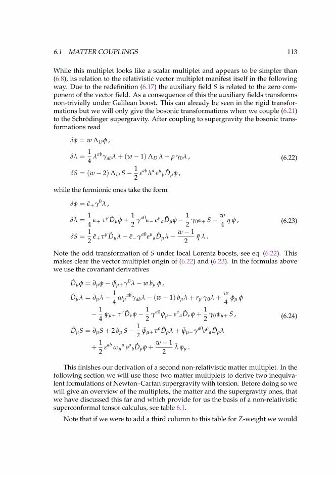
6.1 MATTER COUPLINGS 113
While this multiplet looks like a scalar multiplet and appears to be simpler than(6.8), its relation to the relativistic vector multiplet manifest itself in the followingway. Due to the redefinition (6.17) the auxiliary field S is related to the zero com-ponent of the vector field. As a consequence of this the auxiliary fields transformsnon-trivially under Galilean boost. This can already be seen in the rigid transfor-mations but we will only give the bosonic transformations when we couple (6.21)to the Schrodinger supergravity. After coupling to supergravity the bosonic trans-formations read
δφ = w ΛDφ ,
δλ =14
λabγabλ + (w− 1)ΛD λ− ρ γ0λ ,
δS = (w− 2)ΛD S− 12
εabλa eµbDµφ ,
(6.22)
while the fermionic ones take the form
δφ = ε+γ0λ ,
δλ =14
ε+ τµDµφ +12
γa0ε− eµaDµφ− 1
2γ0ε+ S− w
4η φ ,
δS =12
ε+τµDµλ− ε−γa0eµaDµλ− w− 1
2η λ .
(6.23)
Note the odd transformation of S under local Lorentz boosts, see eq. (6.22). Thismakes clear the vector multiplet origin of (6.22) and (6.23). In the formulas abovewe use the covariant derivatives
Dµφ = ∂µφ− ψµ+γ0λ− w bµ φ ,
Dµλ = ∂µλ− 14
ωµabγabλ− (w− 1) bµλ + rµ γ0λ +
w4
φµ φ
− 14
ψµ+ τνDνφ− 12
γa0ψµ− eνaDνφ +
12
γ0ψµ+ S ,
DµS = ∂µS + 2 bµ S− 12
ψµ+τρDρλ + ψµ−γa0eρaDρλ
+12
εab ωµa eρ
bDρφ +w− 1
2λ φµ .
(6.24)
This finishes our derivation of a second non-relativistic matter multiplet. In thefollowing section we will use those two matter multiplets to derive two inequiva-lent formulations of Newton–Cartan supergravity with torsion. Before doing so wewill give an overview of the multiplets, the matter and the supergravity ones, thatwe have discussed this far and which provide for us the basis of a non-relativisticsuperconformal tensor calculus, see table 6.1.
Note that if we were to add a third column to this table for Z-weight we would
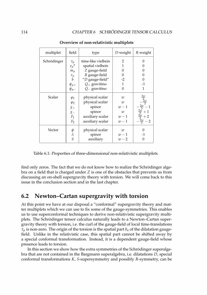
114 CHAPTER 6 SCHRODINGER TENSOR CALCULUS
Overview of non-relativistic multiplets
multiplet field type D-weight R-weight
Schrodinger τµ time-like vielbein 2 0eµ
a spatial vielbein 1 0mµ Z gauge-field 0 0rµ R gauge-field 0 0b “D gauge-field” -2 0
ψµ+ Q+ gravitino 1 -1ψµ− Q− gravitino 0 1
Scalar ϕ1 physical scalar w 2w3
ϕ2 physical scalar w − 2w3
χ+ spinor w− 1 − 2w3 − 1
χ− spinor w 2w3 + 1
F1 auxiliary scalar w− 1 2w3 + 2
F2 auxiliary scalar w− 1 − 2w3 − 2
Vector φ physical scalar w 0λ spinor w− 1 -1S auxiliary w− 2 0
Table 6.1: Properties of three-dimensional non-relativistic multiplets.
find only zeros. The fact that we do not know how to realize the Schrodinger alge-bra on a field that is charged under Z is one of the obstacles that prevents us fromdiscussing an on-shell supergravity theory with torsion. We will come back to thisissue in the conclusion section and in the last chapter.
6.2 Newton–Cartan supergravity with torsionAt this point we have at our disposal a “conformal” supergravity theory and mat-ter multiplets which we can use to fix some of the gauge-symmetries. This enablesus to use superconformal techniques to derive non-relativistic supergravity multi-plets. The Schrodinger tensor calculus naturally leads to a Newton–Cartan super-gravity theory with torsion, i.e. the curl of the gauge-field of local time-translationsτµ is non-zero. The origin of the torsion is the spatial part ba of the dilatation gauge-field. Unlike in the relativistic case, this spatial part cannot be shifted away bya special conformal transformation. Instead, it is a dependent gauge-field whosepresence leads to torsion.
In this section we show how the extra symmetries of the Schrodinger superalge-bra that are not contained in the Bargmann superalgebra, i.e. dilatations D, specialconformal transformations K, S-supersymmetry and possibly R-symmetry, can be
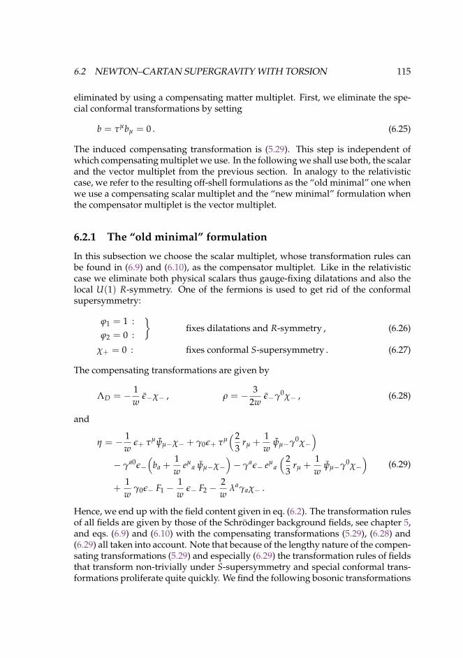
6.2 NEWTON–CARTAN SUPERGRAVITY WITH TORSION 115
eliminated by using a compensating matter multiplet. First, we eliminate the spe-cial conformal transformations by setting
b = τµbµ = 0 . (6.25)
The induced compensating transformation is (5.29). This step is independent ofwhich compensating multiplet we use. In the following we shall use both, the scalarand the vector multiplet from the previous section. In analogy to the relativisticcase, we refer to the resulting off-shell formulations as the “old minimal” one whenwe use a compensating scalar multiplet and the “new minimal” formulation whenthe compensator multiplet is the vector multiplet.
6.2.1 The “old minimal” formulation
In this subsection we choose the scalar multiplet, whose transformation rules canbe found in (6.9) and (6.10), as the compensator multiplet. Like in the relativisticcase we eliminate both physical scalars thus gauge-fixing dilatations and also thelocal U(1) R-symmetry. One of the fermions is used to get rid of the conformalsupersymmetry:
ϕ1 = 1 :ϕ2 = 0 :
fixes dilatations and R-symmetry , (6.26)
χ+ = 0 : fixes conformal S-supersymmetry . (6.27)
The compensating transformations are given by
ΛD = − 1w
ε−χ− , ρ = − 32w
ε−γ0χ− , (6.28)
and
η = − 1w
ε+ τµψµ−χ− + γ0ε+ τµ(2
3rµ +
1w
ψµ−γ0χ−)
− γa0ε−(
ba +1w
eµa ψµ−χ−
)− γaε− eµ
a
(23
rµ +1w
ψµ−γ0χ−)
+1w
γ0ε− F1 −1w
ε− F2 −2w
λaγaχ− .
(6.29)
Hence, we end up with the field content given in eq. (6.2). The transformation rulesof all fields are given by those of the Schrodinger background fields, see chapter 5,and eqs. (6.9) and (6.10) with the compensating transformations (5.29), (6.28) and(6.29) all taken into account. Note that because of the lengthy nature of the compen-sating transformations (5.29) and especially (6.29) the transformation rules of fieldsthat transform non-trivially under S-supersymmetry and special conformal trans-formations proliferate quite quickly. We find the following bosonic transformations
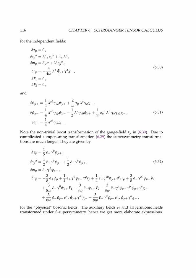
116 CHAPTER 6 SCHRODINGER TENSOR CALCULUS
for the independent fields:
δτµ = 0 ,
δeµa = λa
b eµb + τµ λa ,
δmµ = ∂µσ + λaeµa ,
δrµ = − 34w
λa ψµ+γaχ− ,
δF1 = 0 ,δF2 = 0 ,
(6.30)
and
δψµ+ =14
λabγabψµ+ +2w
τµ λaγaχ− ,
δψµ− =14
λabγabψµ− −12
λaγa0ψµ+ +1w
eµa λb γaγb0χ− ,
δχ− =14
λabγabχ− .
(6.31)
Note the non-trivial boost transformation of the gauge-field rµ in (6.30). Due tocomplicated compensating transformation (6.29) the supersymmetry transforma-tions are much longer. They are given by
δτµ =12
ε+γ0ψµ+ ,
δeµa =
12
ε+γaψµ− +12
ε−γaψµ+ ,
δmµ = ε−γ0ψµ− ,
δrµ = −38
ε+φµ +14
ε+γ0ψµ+ τρrρ +14
ε−γa0ψµ+ eρarρ +
38
ε−γa0ψµ+ ba
+3
8wε−γ0ψµ+ F1 −
38w
ε−ψµ+ F2 −3
8wε+γaψρ− τρ ψµ+γaχ−
+3
8wε−ψρ− eρ
a ψµ+γa0χ− −3
8wε−γ0ψρ− eρ
a ψµ+γaχ− ,
(6.32)
for the “physical” bosonic fields. The auxiliary fields Fi and all fermionic fieldstransformed under S-supersymmetry, hence we get more elaborate expressions.
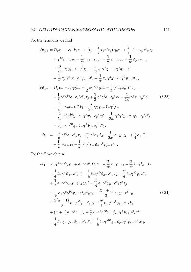
6.2 NEWTON–CARTAN SUPERGRAVITY WITH TORSION 117
For the fermions we find
δψµ+ = Dµε+ − eµa ba ε+ +
(rµ −
23
τµτρrρ
)γ0ε+ +
23
γaε− τµ eρa rρ
+ γa0ε− τµ ba −1w
γ0ε− τµ F1 +1w
ε− τµ F2 −1w
ψµ+ ε−χ−
+3
2wγ0ψµ+ ε−γ0χ− +
1w
τµ γaχ− ε+γaψρ− τρ
− 1w
τµ γa0χ− ε−ψρ− eρa +
1w
τµ γaχ− ε−γ0ψρ− eρa ,
δψµ− = Dµε− − rµ γ0ε− +12
ωµaγa0ε+ −
13
γaε+ eµaτρ rρ
− 13
γaγb0ε+ eµaeρ
b rρ +12
γaγbε− eµa bb −
12w
γaε− eµa F1
− 12w
γa0ε− eµa F2 −
32w
γ0ψµ− ε−γ0χ−
− 12w
γaγb0χ− ε+γbψρ− eµa τρ − 1
2wγaγbχ− ε−ψρ− eµ
aeρb
− 12w
γaγb0χ− ε−γ0ψρ− eµaeρ
b ,
δχ− = −w6
γa0ε+ eµa rµ −
w4
γaε+ ba −1
3wε− χ−χ− +
14
ε+ F1
− 14
γ0ε+ F2 −14
γaγbχ− ε+γbψµ− eµa .
(6.33)
For the Fi we obtain
δF1 = ε+γ0τµDµχ− + ε−γaeµaDµχ− +
2w
ε−χ− F1 −2w
ε−γ0χ− F2
− 14
ε+γaψµ− eµa F1 +
14
ε+γa0ψµ− eµa F2 +
w4
ε+γa0φµ eµa
+12
ε+γaγb0χ− eµa ωµ
b − w6
ε+γaψµ+ eµaτρ rρ
− w6
ε+γaγb0ψµ− eµaeρ
b rρ +2(w + 1)
3ε+χ− τµ rµ
− 2(w + 1)3
ε−γa0χ− eµa rµ +
w4
ε+γaγbψµ− eµa bb
+ (w + 1) ε−γaχ− ba +14
ε+γaγb0χ− ψρ−γbψµ+ eµaτρ
− 14
ε+χ− ψρ−ψµ− eµaeρ
a +14
ε+γab0χ− ψρ−γ0ψµ− eµaeρ
b ,
(6.34)
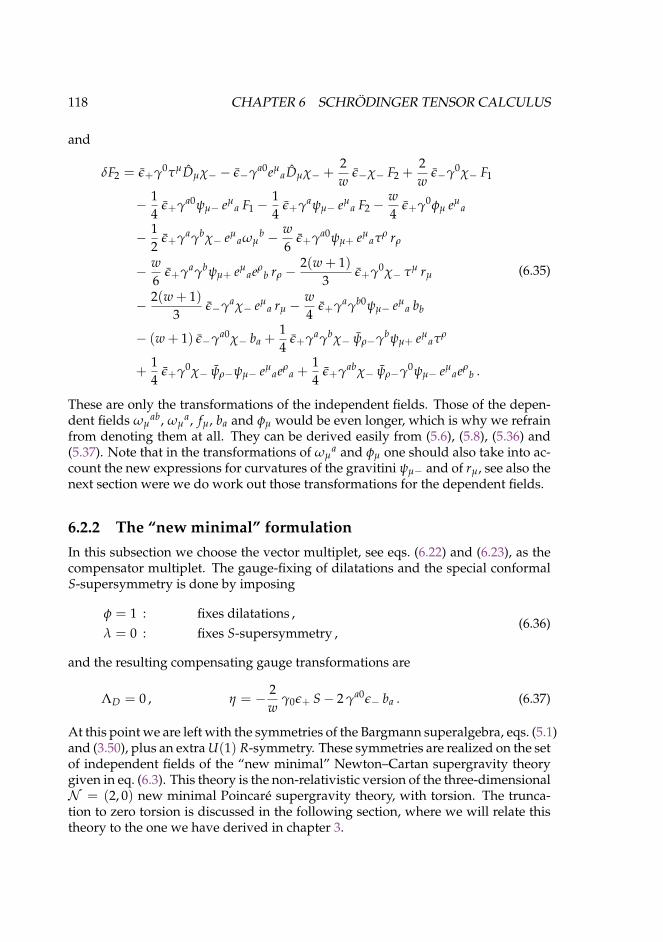
118 CHAPTER 6 SCHRODINGER TENSOR CALCULUS
and
δF2 = ε+γ0τµDµχ− − ε−γa0eµaDµχ− +
2w
ε−χ− F2 +2w
ε−γ0χ− F1
− 14
ε+γa0ψµ− eµa F1 −
14
ε+γaψµ− eµa F2 −
w4
ε+γ0φµ eµa
− 12
ε+γaγbχ− eµaωµ
b − w6
ε+γa0ψµ+ eµaτρ rρ
− w6
ε+γaγbψµ+ eµaeρ
b rρ −2(w + 1)
3ε+γ0χ− τµ rµ
− 2(w + 1)3
ε−γaχ− eµa rµ −
w4
ε+γaγb0ψµ− eµa bb
− (w + 1) ε−γa0χ− ba +14
ε+γaγbχ− ψρ−γbψµ+ eµaτρ
+14
ε+γ0χ− ψρ−ψµ− eµaeρ
a +14
ε+γabχ− ψρ−γ0ψµ− eµaeρ
b .
(6.35)
These are only the transformations of the independent fields. Those of the depen-dent fields ωµ
ab, ωµa, fµ, ba and φµ would be even longer, which is why we refrain
from denoting them at all. They can be derived easily from (5.6), (5.8), (5.36) and(5.37). Note that in the transformations of ωµ
a and φµ one should also take into ac-count the new expressions for curvatures of the gravitini ψµ− and of rµ, see also thenext section were we do work out those transformations for the dependent fields.
6.2.2 The “new minimal” formulationIn this subsection we choose the vector multiplet, see eqs. (6.22) and (6.23), as thecompensator multiplet. The gauge-fixing of dilatations and the special conformalS-supersymmetry is done by imposing
φ = 1 : fixes dilatations ,λ = 0 : fixes S-supersymmetry ,
(6.36)
and the resulting compensating gauge transformations are
ΛD = 0 , η = − 2w
γ0ε+ S− 2 γa0ε− ba . (6.37)
At this point we are left with the symmetries of the Bargmann superalgebra, eqs. (5.1)and (3.50), plus an extra U(1) R-symmetry. These symmetries are realized on the setof independent fields of the “new minimal” Newton–Cartan supergravity theorygiven in eq. (6.3). This theory is the non-relativistic version of the three-dimensionalN = (2, 0) new minimal Poincare supergravity theory, with torsion. The trunca-tion to zero torsion is discussed in the following section, where we will relate thistheory to the one we have derived in chapter 3.
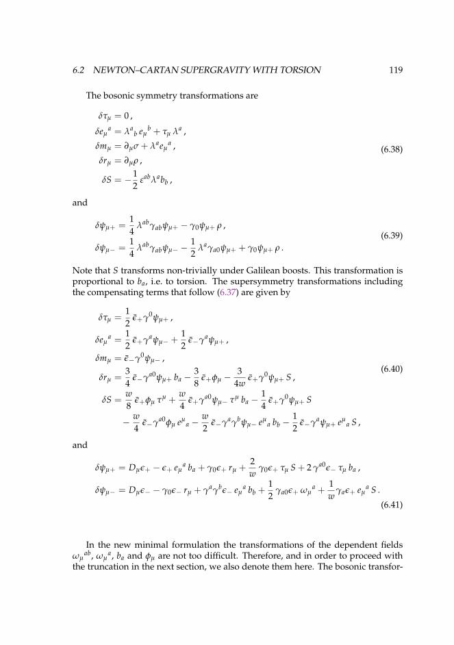
6.2 NEWTON–CARTAN SUPERGRAVITY WITH TORSION 119
The bosonic symmetry transformations are
δτµ = 0 ,
δeµa = λa
b eµb + τµ λa ,
δmµ = ∂µσ + λaeµa ,
δrµ = ∂µρ ,
δS = −12
εabλabb ,
(6.38)
and
δψµ+ =14
λabγabψµ+ − γ0ψµ+ ρ ,
δψµ− =14
λabγabψµ− −12
λaγa0ψµ+ + γ0ψµ+ ρ .(6.39)
Note that S transforms non-trivially under Galilean boosts. This transformation isproportional to ba, i.e. to torsion. The supersymmetry transformations includingthe compensating terms that follow (6.37) are given by
δτµ =12
ε+γ0ψµ+ ,
δeµa =
12
ε+γaψµ− +12
ε−γaψµ+ ,
δmµ = ε−γ0ψµ− ,
δrµ =34
ε−γa0ψµ+ ba −38
ε+φµ −3
4wε+γ0ψµ+ S ,
δS =w8
ε+φµ τµ +w4
ε+γa0ψµ− τµ ba −14
ε+γ0ψµ+ S
− w4
ε−γa0φµ eµa −
w2
ε−γaγbψµ− eµa bb −
12
ε−γaψµ+ eµa S ,
(6.40)
and
δψµ+ = Dµε+ − ε+ eµa ba + γ0ε+ rµ +
2w
γ0ε+ τµ S + 2 γa0ε− τµ ba ,
δψµ− = Dµε− − γ0ε− rµ + γaγbε− eµa bb +
12
γa0ε+ ωµa +
1w
γaε+ eµa S .
(6.41)
In the new minimal formulation the transformations of the dependent fieldsωµ
ab, ωµa, ba and φµ are not too difficult. Therefore, and in order to proceed with
the truncation in the next section, we also denote them here. The bosonic transfor-

120 CHAPTER 6 SCHRODINGER TENSOR CALCULUS
mations are
δωµab = ∂µλab ,
δωµa = ∂µλa −ωµ
abλb + λa eµb bb + eµ
aλb bb + λab ωµ
b ,
δba = λab bb ,
δφµ =14
λabγabφµ − γ0φµ ρ− ψµ+ λa ba .
(6.42)
and
δωµab = −1
4ε+γab0φµ +
12w
ε+γabψµ+ S + ε−γ[aψµ+ bb] ,
δωµa = ε−γ0ψµ
a− +
14
eµb ε+γbψa
0− +14
ε+γaψµ0− −1w
ε+γa0ψµ− S
− 1w
ε−γa0ψµ+ S− 2 εab ε−ψµ− bb + eµbeρ
a ε−γ0γbγcψρ− bc
− 12
eµbeρ
a ε−γb(φρ +2w
γ0ψρ+ S)+
12
eµa τρ ε+γbψρ+ bb ,
δba = −12
ε+γbψµ− eµb ba −
12
ε+γ0ψµ+ τµ ba −14
ε+γ0φµ eµa
− 12w
ε+ψµ+ eµa S ,
δφµ = ε+ fµ −23
γ0ε+[Rµ0(R) +
32
τν ψ[µ−γa0ψν]+ ba −3
4wτν ψ[µ+γ0ψν]+ S
]+
43
γaε−[Rµa(R) +
32
eνa ψ[µ−γb0ψν]+ bb −
34w
eνa ψ[µ+γ0ψν]+ S
]−(
Dµ + eµa ba + rµ γ0
)( 2w
γ0ε+ S + 2 γb0ε− bb)
.
(6.43)
Here, we used the covariant curvatures of the independent gauge-fields ψµ− andrµ, which are
ψµν− = 2 ∂[µψν]− −12
ω[µabγabψν]− − 2 r[µ γ0ψν]− + ω[µ
a γa0ψν]+
+ 2 γaγbψ[ν− eµ]abb +
2w
γaψ[ν+ eµ]a S ,
Rµν(R) = 2 ∂[µrν] +34
ψ[µ+φν] −32
ψ[µ−γa0ψν]+ ba +3
4wψ[µ+γ0ψν]+ S .
(6.44)
The expression for the special conformal gauge-field fµ can be found in (5.35). Wedid not derive its transformation rule because no independent field transforms tofµ and therefore its variation is not needed for any checks on e.g. closure of thecommutator algebra.
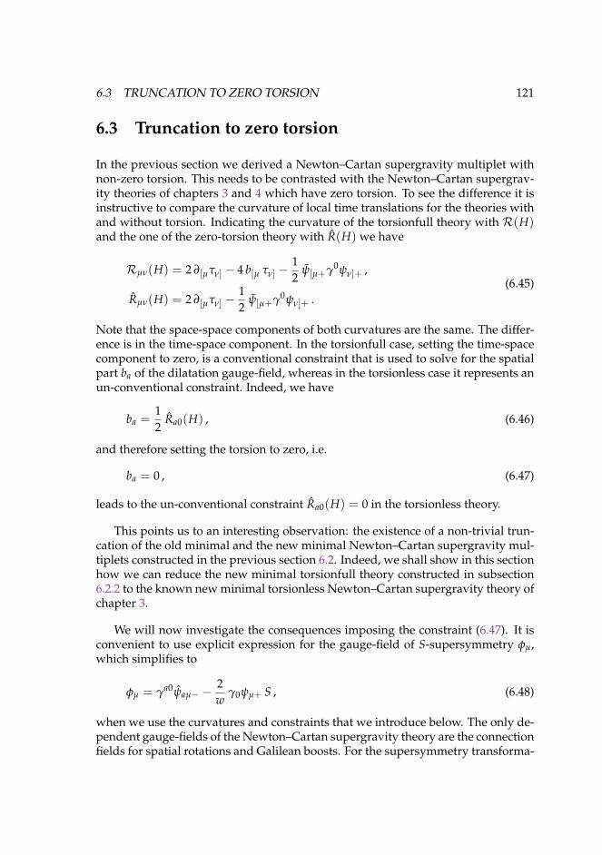
6.3 TRUNCATION TO ZERO TORSION 121
6.3 Truncation to zero torsion
In the previous section we derived a Newton–Cartan supergravity multiplet withnon-zero torsion. This needs to be contrasted with the Newton–Cartan supergrav-ity theories of chapters 3 and 4 which have zero torsion. To see the difference it isinstructive to compare the curvature of local time translations for the theories withand without torsion. Indicating the curvature of the torsionfull theory with R(H)and the one of the zero-torsion theory with R(H) we have
Rµν(H) = 2 ∂[µτν] − 4 b[µ τν] −12
ψ[µ+γ0ψν]+ ,
Rµν(H) = 2 ∂[µτν] −12
ψ[µ+γ0ψν]+ .(6.45)
Note that the space-space components of both curvatures are the same. The differ-ence is in the time-space component. In the torsionfull case, setting the time-spacecomponent to zero, is a conventional constraint that is used to solve for the spatialpart ba of the dilatation gauge-field, whereas in the torsionless case it represents anun-conventional constraint. Indeed, we have
ba =12
Ra0(H) , (6.46)
and therefore setting the torsion to zero, i.e.
ba = 0 , (6.47)
leads to the un-conventional constraint Ra0(H) = 0 in the torsionless theory.
This points us to an interesting observation: the existence of a non-trivial trun-cation of the old minimal and the new minimal Newton–Cartan supergravity mul-tiplets constructed in the previous section 6.2. Indeed, we shall show in this sectionhow we can reduce the new minimal torsionfull theory constructed in subsection6.2.2 to the known new minimal torsionless Newton–Cartan supergravity theory ofchapter 3.
We will now investigate the consequences imposing the constraint (6.47). It isconvenient to use explicit expression for the gauge-field of S-supersymmetry φµ,which simplifies to
φµ = γa0ψaµ− −2w
γ0ψµ+ S , (6.48)
when we use the curvatures and constraints that we introduce below. The only de-pendent gauge-fields of the Newton–Cartan supergravity theory are the connectionfields for spatial rotations and Galilean boosts. For the supersymmetry transforma-
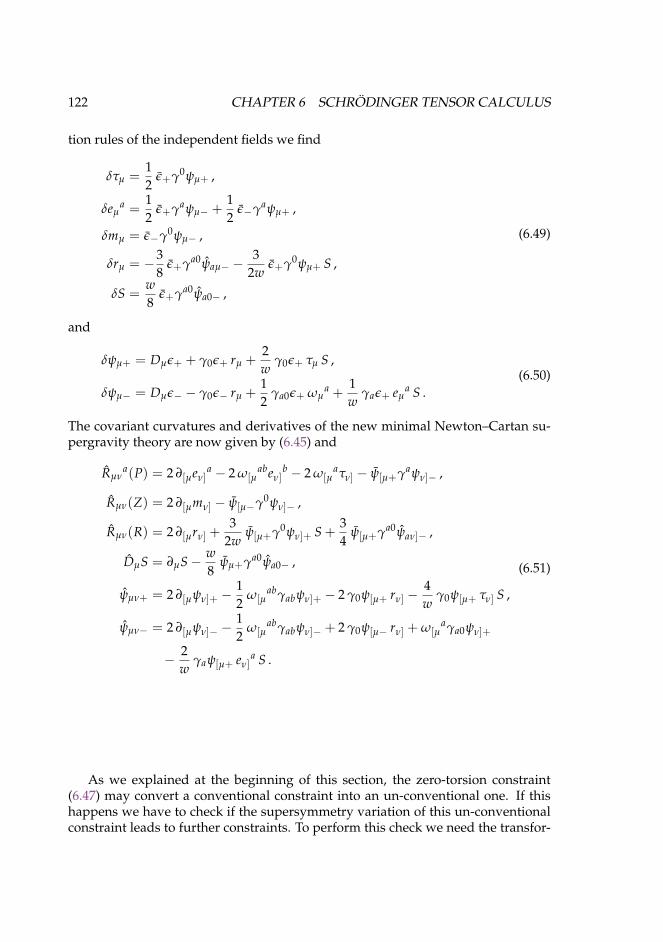
122 CHAPTER 6 SCHRODINGER TENSOR CALCULUS
tion rules of the independent fields we find
δτµ =12
ε+γ0ψµ+ ,
δeµa =
12
ε+γaψµ− +12
ε−γaψµ+ ,
δmµ = ε−γ0ψµ− ,
δrµ = −38
ε+γa0ψaµ− −3
2wε+γ0ψµ+ S ,
δS =w8
ε+γa0ψa0− ,
(6.49)
and
δψµ+ = Dµε+ + γ0ε+ rµ +2w
γ0ε+ τµ S ,
δψµ− = Dµε− − γ0ε− rµ +12
γa0ε+ ωµa +
1w
γaε+ eµa S .
(6.50)
The covariant curvatures and derivatives of the new minimal Newton–Cartan su-pergravity theory are now given by (6.45) and
Rµνa(P) = 2 ∂[µeν]
a − 2 ω[µabeν]
b − 2 ω[µaτν] − ψ[µ+γaψν]− ,
Rµν(Z) = 2 ∂[µmν] − ψ[µ−γ0ψν]− ,
Rµν(R) = 2 ∂[µrν] +3
2wψ[µ+γ0ψν]+ S +
34
ψ[µ+γa0ψaν]− ,
DµS = ∂µS− w8
ψµ+γa0ψa0− ,
ψµν+ = 2 ∂[µψν]+ −12
ω[µabγabψν]+ − 2 γ0ψ[µ+ rν] −
4w
γ0ψ[µ+ τν] S ,
ψµν− = 2 ∂[µψν]− −12
ω[µabγabψν]− + 2 γ0ψ[µ− rν] + ω[µ
aγa0ψν]+
− 2w
γaψ[µ+ eν]a S .
(6.51)
As we explained at the beginning of this section, the zero-torsion constraint(6.47) may convert a conventional constraint into an un-conventional one. If thishappens we have to check if the supersymmetry variation of this un-conventionalconstraint leads to further constraints. To perform this check we need the transfor-
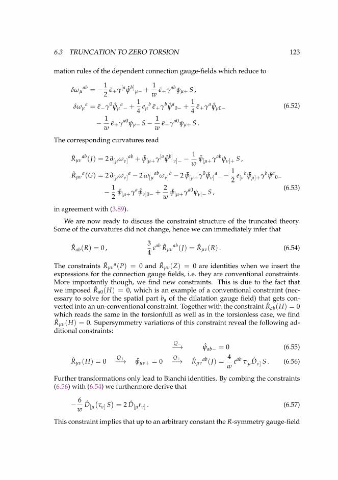
6.3 TRUNCATION TO ZERO TORSION 123
mation rules of the dependent connection gauge-fields which reduce to
δωµab = −1
2ε+γ[aψb]
µ− +1w
ε+γabψµ+ S ,
δωµa = ε−γ0ψµ
a− +
14
eµb ε+γbψa
0− +14
ε+γaψµ0−
− 1w
ε+γa0ψµ− S− 1w
ε−γa0ψµ+ S .
(6.52)
The corresponding curvatures read
Rµνab(J) = 2 ∂[µων]
ab + ψ[µ+γ[aψb]ν]− −
1w
ψ[µ+γabψν]+ S ,
Rµνa(G) = 2 ∂[µων]
a − 2 ω[µabων]
b − 2 ψ[µ−γ0ψν]a− −
12
e[νbψµ]+γbψa
0−
− 12
ψ[µ+γaψν]0− +2w
ψ[µ+γa0ψν]− S ,(6.53)
in agreement with (3.89).
We are now ready to discuss the constraint structure of the truncated theory.Some of the curvatures did not change, hence we can immediately infer that
Rab(R) = 0 ,34
εab Rµνab(J) = Rµν(R) . (6.54)
The constraints Rµνa(P) = 0 and Rµν(Z) = 0 are identities when we insert the
expressions for the connection gauge fields, i.e. they are conventional constraints.More importantly though, we find new constraints. This is due to the fact thatwe imposed Ra0(H) = 0, which is an example of a conventional constraint (nec-essary to solve for the spatial part ba of the dilatation gauge field) that gets con-verted into an un-conventional constraint. Together with the constraint Rab(H) = 0which reads the same in the torsionfull as well as in the torsionless case, we findRµν(H) = 0. Supersymmetry variations of this constraint reveal the following ad-ditional constraints:
Q−−→ ψab− = 0 (6.55)
Rµν(H) = 0Q+−→ ψµν+ = 0
Q+−→ Rµνab(J) =
4w
εab τ[µDν] S . (6.56)
Further transformations only lead to Bianchi identities. By combing the constraints(6.56) with (6.54) we furthermore derive that
− 6w
D[µ
(τν] S
)= 2 D[µrν] . (6.57)
This constraint implies that up to an arbitrary constant the R-symmetry gauge-field
124 CHAPTER 6 SCHRODINGER TENSOR CALCULUS
rµ is determined by τµ and S. In fact, when we set
rµ = − 3w
τµ S , (6.58)
the truncated theory precisely leads to the off-shell Newton–Cartan multiplet thatwas presented in chapter 3. Furthermore, by making the redefinition
rµ = −Vµ −1w
τµ S , (6.59)
one obtains precisely the off-shell multiplet that was obtained when taking the limitof the new minimal Poincare multiplet.
6.4 A brief summaryThis chapter served various purposes. We introduced matter multiplets and thusshowed how we can couple non-relativistic matter to non-relativistic supergrav-ity backgrounds. Secondly, we derived another generalization of Newton–Cartansupergravity, namely the theory with torsion. Lastly, we showed that there is noobstacle in taking over the ideas of the superconformal tensor calculus used in therelativistic setting and applying them to our non-relativistic supergravity theories.
Note that we did not derive an on-shell Newton–Cartan supergravity theorywith torsion. It would be interesting to see how one can go on-shell in the presenceof torsion. Unlike the truncation to zero torsion that we performed in section 6.3this is not a straightforward thing to do. The problem is that even in the bosoniccase the equations of motion describing Newton–Cartan gravity with torsion havenot been written down so far.3 Even in the absence of torsion the equations ofmotion have only been written down under the assumption that the curvature ofspatial rotations is zero [80]. It is not difficult to write down the equations of motionfor the case that this curvature is nonzero but the price one has to pay is that onehas to add extra terms to the equation of motion proposed in [80] that break theinvariance under central charge transformations [29]. In the non-relativistic super-conformal approach we are using in this work this requires the introduction of twocompensating scalars: one for dilatations and one for the central charge transforma-tions. Unlike the compensating scalar for dilatations, the compensating scalar forcentral charge transformations should transform non-trivially under central chargetransformations and hence should be part of a different multiplet. The construc-tion of such a multiplet is different from our investigations in section 6.1 and goesbeyond the scope of this thesis.
3 A systematic approach to construct such an equation of motion is part of the analysis in [102].
7Conclusion
In this chapter we will recap the results that we have obtained and take anotherlook at generalizations and extensions thereof. For a large part this will be buta repetition of the outlook given in each of the previous chapters.
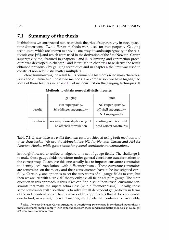
126 CHAPTER 7 CONCLUSION
7.1 Summary of the thesisIn this thesis we constructed non-relativistic theories of supergravity in three space-time dimensions. Two different methods were used for that purpose. Gaugingtechniques, which are known to provide one way towards supergravity in the rela-tivistic case [95], and which were used in the derivation of the first Newton–Cartansupergravity too, featured in chapters 4 and 5. A limiting and contraction proce-dure was developed in chapter 3 and later used in chapter 4 to re-derive the resultobtained previously by gauging techniques and in chapter 6 the limit was used toconstruct non-relativistic matter multiplets.
Before summarizing the result let us comment a bit more on the main character-istics and differences of those two methods. For comparison, we have highlightedsome of those features in table 7.1. Let us focus first on the gauging techniques. It
Methods to obtain non-relativistic theories
gauging limit
NH supergravity, NC (super-)gravity,
results Schrodinger supergravity, off-shell supergravity,
NH supergravity,
drawbacks not easy: close algebra on g.c.t. starting point is crucial
no off-shell formulation need correct constraints
Table 7.1: In this table we enlist the main results achieved using both methods andtheir drawbacks. We use the abbreviations NC for Newton–Cartan and NH forNewton–Hooke, while g.c.t. stands for general coordinate transformations.
is straightforward to realize an algebra on a set of gauge-fields. The challenge isto make those gauge-fields transform under general coordinate transformations inthe correct way. To achieve this one usually has to imposes curvature constraintsto identify local translations with diffeomorphisms. These curvature constraintsare constraints on the theory and their consequences have to be investigated care-fully. Certainly, one option is to set the curvatures of all gauge-fields to zero, butthen we are left with a “trivial” theory only, i.e. all fields are pure gauge. The mainquestion in this approach is thus if we can find a set of non-trivial curvature con-straints that make the superalgebra close (with diffeomorphisms).1 Ideally, thosesame constraints will also allow us to solve for all dependent gauge-fields in termsof the independent ones. The drawback of this approach is that it does not enableone to find, in a straightforward manner, multiplets that contain auxiliary fields.
1 Also, if we use Newton–Cartan structures to describe e.g. phenomena in condensed matter theory,these constraints should comply with expectations from those condensed matter models, e.g. we mightnot want to set torsion to zero.

7.1 SUMMARY OF THE THESIS 127
However, as we showed in chapter 6, Schrodinger techniques might be one optionto circumvent this obstacle.
In conclusion, the starting point here is easy and the difficulty lies in convertingthis into a geometric theory. We should also point out that, while we sometimesmade use of both techniques, ultimately all supergravity theories in this thesis werederived using gauging techniques.
In contrast, the difficulty of the limiting procedure lies in finding the correctstarting point. From then on, one just needs to apply the procedure and see whatit leads to. It might just be that one finds the limit does not work. For example, inorder to avoid divergent terms when taking the limit, we might be forced to puttoo many constraints on the independent fields of the theory. Then, one could tryto tweak the starting point, or one must deduce that the theory under considerationdoes not have this kind of non-relativistic limit.
Let us now turn to the results that we have obtained. To provide an overviewover the different non-relativistic supergravity theories discussed in this thesis wesummarize them in table 7.2. The first line, on-shell Newton–Cartan supergravity,
Overview of supergravities
field content limit of algebra gauged
NC τµ, eµa, mµ, ψµ± on-shell Poincare N = 2 Bargmann
off-shell NC NC plus S new minimal multiplet (N = 2 Bargmann)
NH NC AdS supergravity N = (2, 0) NH
Schrodinger NC plus rµ no limit Schrodinger
TNC “old” NC plus rµ, F1, F2, χ no limit (known) (N = 2 Bargmann)
TNC “new” NC plus rµ, S no limit (known) (N = 2 Bargmann)
Table 7.2: In this table we review the non-relativistic supergravities of this thesisand some of their features. The abbreviations NC, NH and AdS stand for Newton–Cartan, Newton–Hooke and anti-de Sitter, respectively. TNC “old”/“new” referto the old/new minimal formulation of Newton–Cartan supergravity with torsion.The algebras in brackets indicate that the theory is not obtained by gauging tech-niques, but nevertheless realizes this algebra.
is the first example of a theory of non-relativistic supergravity. This thesis is verymuch built on that result and aimed to generalize it in various directions, whichwe have depicted in figure 1.2 in the introduction. Our generalizations given inthe first column of table 7.2, comprise the following extentions. The cosmologicalextension that we called Newton–Hooke supergravity featured in chapter 4. A“conformal” extension that we dubbed Schrodinger supergravity was presentedin chapter 5. Finally, an extension with non-vanishing torsion and two novel off-
128 CHAPTER 7 CONCLUSION
shell formulations of the original Newton–Cartan supergravity theory of [77] werethe subject of chapter 6 (and also chapter 3).
The field content of the various theories, given in the second column of table7.2, always consists of(
τµ, eµa, mµ, ψµ±
)+ more , (7.1)
i.e. at least the fields of on-shell Newton–Cartan supergravity. Several extensionsthen include more fields which are either auxiliary, or in the case of Schrodingersupergravity where there are more symmetries, extra gauge-fields. Recall that weargued in chapter 6 that one can eliminate the gauge-field rµ (we also used thenotation Vµ) of R-symmetry when considering the truncation to zero torsion of thenew minimal formulation. Thus, the difference in field content of the two newminimal formulations in line two and six of table 7.2.
In those cases where we also discussed the connection to a relativistic theory,via the limiting procedure, we indicated this “parent” theory in the third columnof table 7.2. As we mentioned in chapter 5 there is no way to apply the limitingprocedure in the case for Schrodinger supergravity. In contrast, we do not claimthat no such limit exists for the torsional Newton–Cartan supergravity theories.However, taking the limit as discussed in chapter 3, especially for the new minimaltheory, imposes that the theory be torsionless. Therefore we did not indicate relatedrelativistic theories here.
The purpose of the last column is to depict the symmetry algebra that the multi-plet realizes. In most cases that means that this theory is obtained by gauging saidalgebra, as shown in many examples in our work. Only for the off-shell formula-tions this is not possible in a straightforward way.
In hindsight we realize that not all extensions are on the same footing, as suggestedby figure 1.2 in the introduction. Having gone through the gauge-fixings and othertruncations (on-shell/off-shell and torsion/no torsion) in detail in chapter 6, weunderstand the relation between all those extensions much better now. It turns outthat the figure should look more like figure 7.1. The form of this diagram is alsosuggestive of extensions of this work. Can we first go on-shell and then truncateto zero torsion? What is off-shell formulation of Newton–Hooke supergravity? Wecome back to these points in the following section, when we provide an outlook onfuture work.
The construction of non-relativistic (conformal) supergravity enabled us to con-struct non-relativistic matter multiplets too. This was part of our analysis in chapter6, where we also made use of our limiting procedure. Let us repeat part of the tablewhere the field content and weights of the fields of the matter multiplets were sum-marized, see table 7.3. These are the only matter multiplets that we constructed sofar but there are certainly others. Indeed, the construction of one particular mattermultiplet with a (scalar) field that is charged under central charge symmetry is part

7.2 OUTLOOK 129
The relation between the extensions of Newton–Cartan supergravity
Schrodinger supergravity + compensator multiplets
off-shell, torsion-fullNewton–Cartan supergravity
truncation to zero torsion
going on-shell
“original”Newton–Cartan supergravity
cosmological extensions:Newton–Hooke supergravity
Figure 7.1: The relation of the different supergravity theories discussed in this the-sis.
of one very interesting extension of this work. We come back to this issue in thenext section, when discussing in more detail the possible extensions of our work.
Finally, in the last chapter we also showed that the techniques from the supercon-formal tensor calculus can be applied in the non-relativistic setting in a straight-forward way. This enabled us to re-derive and extend all of the previous resultson torsionless supergravities. It also provided a very efficient way to construct tor-sionfull theories.
This finishes our summary of the results that we have obtained in this thesis. In thefollowing, we will expand on possible extensions of this work.
7.2 OutlookTo start, let us come back to some issues which we have just found in the previ-ous section. For example, looking at the table 7.2 we realize that we do not havean on-shell formulation of torsional Newton–Cartan supergravity. The problemhere is that we do not have a compensating matter multiplet that contains a fieldwhich transforms under the central charge symmetry. Remember, if Rµν
ab(J) 6= 0the equation of motion is not invariant under boosts. Say, we add extra terms thatsolve this problem, then we obtain an equation of motion that is not invariant under
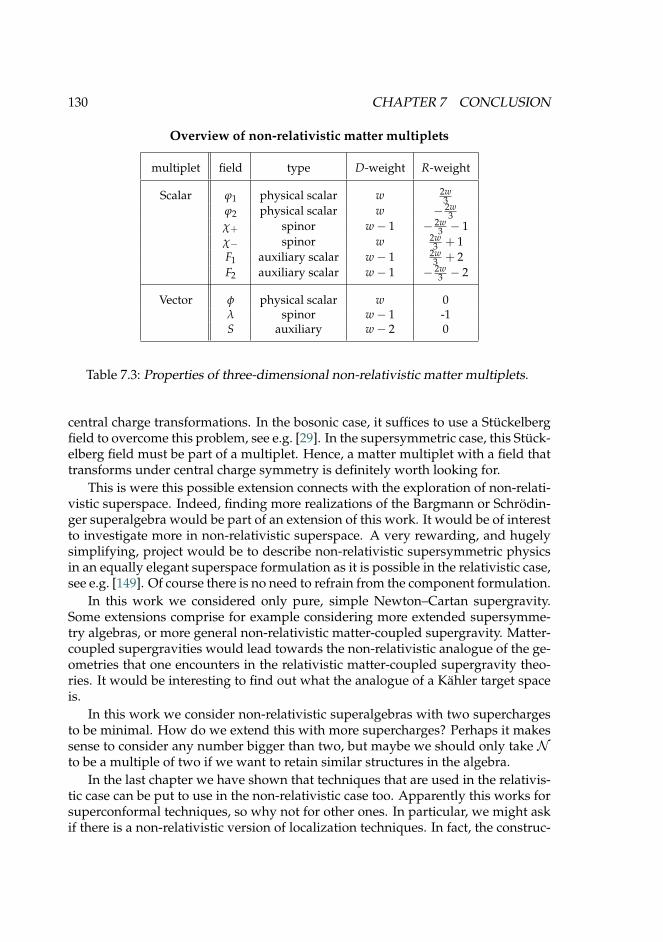
130 CHAPTER 7 CONCLUSION
Overview of non-relativistic matter multiplets
multiplet field type D-weight R-weight
Scalar ϕ1 physical scalar w 2w3
ϕ2 physical scalar w − 2w3
χ+ spinor w− 1 − 2w3 − 1
χ− spinor w 2w3 + 1
F1 auxiliary scalar w− 1 2w3 + 2
F2 auxiliary scalar w− 1 − 2w3 − 2
Vector φ physical scalar w 0λ spinor w− 1 -1S auxiliary w− 2 0
Table 7.3: Properties of three-dimensional non-relativistic matter multiplets.
central charge transformations. In the bosonic case, it suffices to use a Stuckelbergfield to overcome this problem, see e.g. [29]. In the supersymmetric case, this Stuck-elberg field must be part of a multiplet. Hence, a matter multiplet with a field thattransforms under central charge symmetry is definitely worth looking for.
This is were this possible extension connects with the exploration of non-relati-vistic superspace. Indeed, finding more realizations of the Bargmann or Schrodin-ger superalgebra would be part of an extension of this work. It would be of interestto investigate more in non-relativistic superspace. A very rewarding, and hugelysimplifying, project would be to describe non-relativistic supersymmetric physicsin an equally elegant superspace formulation as it is possible in the relativistic case,see e.g. [149]. Of course there is no need to refrain from the component formulation.
In this work we considered only pure, simple Newton–Cartan supergravity.Some extensions comprise for example considering more extended supersymme-try algebras, or more general non-relativistic matter-coupled supergravity. Matter-coupled supergravities would lead towards the non-relativistic analogue of the ge-ometries that one encounters in the relativistic matter-coupled supergravity theo-ries. It would be interesting to find out what the analogue of a Kahler target spaceis.
In this work we consider non-relativistic superalgebras with two superchargesto be minimal. How do we extend this with more supercharges? Perhaps it makessense to consider any number bigger than two, but maybe we should only take Nto be a multiple of two if we want to retain similar structures in the algebra.
In the last chapter we have shown that techniques that are used in the relativis-tic case can be put to use in the non-relativistic case too. Apparently this works forsuperconformal techniques, so why not for other ones. In particular, we might askif there is a non-relativistic version of localization techniques. In fact, the construc-
7.2 OUTLOOK 131
tion of off-shell multiplets throughout this work was an effort in this direction.Off-shell formulations are needed to put (rigid) supergravity on a curved back-ground, see e.g. [76]. So obviously, now that we have those off-shell formulationsone extension can consist of answering the question on what backgrounds we canput a non-relativistic theory of supergravity. In a next step, one can ask if we canapply localization techniques to calculate partition functions for non-relativistic su-persymmetric theories on curved backgrounds.
An equally obvious but probably more “physical” extension would be to go tohigher dimensions. Using techniques presented in this thesis we might aim to con-struct Newton–Cartan supergravity in four space-time dimensions, a goal whichhas remained elusive this far. The limiting procedure put forward in chapter 3might be useful for that purpose.
In fact, one can find several applications for the non-relativistic limiting proce-dure that we developed here. For example, one could set out to derive the non-relativistic string [101] in a way similar to the point-particle limit that we tookin chapter 3. To do so, one would first have to find a suitable extension of thePoincare algebra whose Inonu–Wigner contraction leads to the extended Galilei al-gebra of [64].
The procedure need not be used to take non-relativistic limits only. The basicidea of the limiting procedure goes beyond that. It should be clear from the analysisof chapter 3 that, naively, all we need to perform the limit is the contraction ofone algebra to another one. There possibly exist similar limits that descend fromthe ultra-relativistic contraction of the Poincare algebra, which leads to the Carrollalgebra. Ideally, such a contraction procedure would lead to an ultra-relativisticversion of gravity, such as the theory of Carroll gravity introduced by Hartong [61].Perhaps, such a limit could also be used to derive the Carroll (super-)particle in acurved background, see [59, 60].
It is not clear whether every algebra contraction can be translated into a con-traction at the level of the field theory representing that algebra. Moreover, certainnon-relativistic symmetry algebras cannot be viewed as contractions of relativisticones. An example of such an algebra is given by the Schrodinger algebra. However,the Bargmann and the Schrodinger algebra can be obtained as light-like reductionsof relativistic algebras [150, 151]. Perhaps one can define a different sort of contrac-tion or limiting procedure related to such kind of reductions, which would giverise to (torsional) Newton–Cartan structures as presented in [29, 80]. In view of therecent applications of torsional Newton–Cartan geometry in non-relativistic holog-raphy [15, 25–28], it would be interesting to investigate this case in more detail.
This brings us back to the putative applications of our results in condensed mat-ter theory. Recall that our search for off-shell formulations was motivated by thelong-term goal to investigate localization techniques in the non-relativistic context.If such techniques can indeed be applied, they might prove very useful in yield-ing exact results (partition functions, which lead to response functions, etc. . . ) fornon-relativistic field theories.
For example, one piece of the action of Son’s effective model for the quantum
132 CHAPTER 7 CONCLUSION
Hall effect [30] remains undetermined in that work. As he points out, symmetryarguments certainly restrict the possible terms that can appear as extra contribu-tions to the action. Perhaps requiring supersymmetry can put enough restrictionsto determine the possible terms even more.
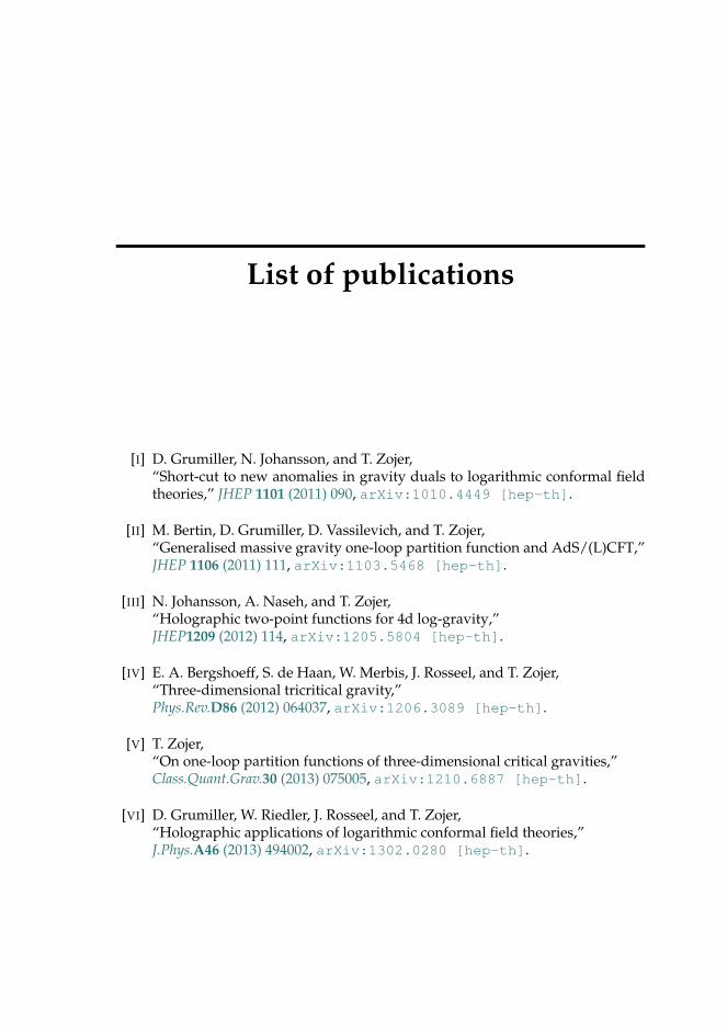
List of publications
[I] D. Grumiller, N. Johansson, and T. Zojer,“Short-cut to new anomalies in gravity duals to logarithmic conformal fieldtheories,” JHEP 1101 (2011) 090, arXiv:1010.4449 [hep-th].
[II] M. Bertin, D. Grumiller, D. Vassilevich, and T. Zojer,“Generalised massive gravity one-loop partition function and AdS/(L)CFT,”JHEP 1106 (2011) 111, arXiv:1103.5468 [hep-th].
[III] N. Johansson, A. Naseh, and T. Zojer,“Holographic two-point functions for 4d log-gravity,”JHEP1209 (2012) 114, arXiv:1205.5804 [hep-th].
[IV] E. A. Bergshoeff, S. de Haan, W. Merbis, J. Rosseel, and T. Zojer,“Three-dimensional tricritical gravity,”Phys.Rev.D86 (2012) 064037, arXiv:1206.3089 [hep-th].
[V] T. Zojer,“On one-loop partition functions of three-dimensional critical gravities,”Class.Quant.Grav.30 (2013) 075005, arXiv:1210.6887 [hep-th].
[VI] D. Grumiller, W. Riedler, J. Rosseel, and T. Zojer,“Holographic applications of logarithmic conformal field theories,”J.Phys.A46 (2013) 494002, arXiv:1302.0280 [hep-th].
134
[VII] E. A. Bergshoeff, M. Kovacevic, L. Parra, J. Rosseel, Y. Yin, and T. Zojer,“New massive supergravity and auxiliary fields,”Class.Quant.Grav. 30 (2013) 195004, arXiv:1304.5445 [hep-th].
[VIII] E. Bergshoeff, M. Kovacevic, L. Parra, and T. Zojer,“A new road to massive gravity?,”PoS Corfu2012 (2013) 053.
[IX] E. Bergshoeff, J. Gomis, M. Kovacevic, L. Parra, J. Rosseel, and T. Zojer,“Non-relativistic superparticle in a curved background,”Phys.Rev.D90 (2014) 065006, arXiv:1406.7286 [hep-th].
[X] E. Bergshoeff, J. Rosseel, and T. Zojer,“Newton–Cartan (super)gravity as a non-relativistic limit,”Class.Quant.Grav. 32 (2015) 205003, arXiv:1505.02095 [hep-th].
[XI] E. Bergshoeff, J. Rosseel, and T. Zojer,“Newton–Cartan supergravity with torsion and Schrodinger supergravity,”JHEP 1511 (2015) 180, arXiv:1509.04527 [hep-th].
References
[1] A. Einstein, “Die Grundlage der allgemeinen Relativitatstheorie,” Annalen der Physik49 (1916) 769–822. (in German).
[2] E. Cartan, “Sur les varietes a connexion affine et la theorie de la relativite generalisee(premiere partie),” Ann. Ecole Norm. Sup. 40 (1923) 325–412. link to full text (inFrench).
[3] E. Cartan, “Sur les varietes a connexion affine et la theorie de la relativite generalisee(premiere partie) (Suite),” Ann. Ecole Norm. Sup. 41 (1924) 1–25. link to full text (inFrench).
[4] C. Duval, “On Galileian isometries,” Class.Quant.Grav. 10 (1993) 2217–2222,arXiv:0903.1641 [math-ph].
[5] D. Son and M. Wingate, “General coordinate invariance and conformal invariance innonrelativistic physics: Unitary Fermi gas,” Annals Phys. 321 (2006) 197–224,arXiv:cond-mat/0509786 [cond-mat].
[6] Y. Nishida and D. T. Son, “Nonrelativistic conformal field theories,” Phys.Rev. D76(2007) 086004, arXiv:0706.3746 [hep-th].
[7] D. Son, “Toward an AdS/cold atoms correspondence: A Geometric realization of theSchrodinger symmetry,” Phys.Rev. D78 (2008) 046003, arXiv:0804.3972[hep-th].
[8] M. Geracie, D. T. Son, C. Wu, and S.-F. Wu, “Spacetime Symmetries of the QuantumHall Effect,” Phys.Rev. D91 (2015) 045030, arXiv:1407.1252[cond-mat.mes-hall].
[9] B. Bradlyn and N. Read, “Low-energy effective theory in the bulk for transport in atopological phase,” Phys. Rev. B91 (2015) 125303, arXiv:1407.2911[cond-mat.mes-hall].
[10] T. Brauner, S. Endlich, A. Monin, and R. Penco, “General coordinate invariance inquantum many-body systems,” Phys. Rev. D90 (2014) 105016, arXiv:1407.7730[hep-th].

136 REFERENCES
[11] K. Jensen, “On the coupling of Galilean-invariant field theories to curved spacetime,”arXiv:1408.6855 [hep-th].
[12] K. Jensen, “Aspects of hot Galilean field theory,” JHEP 1504 (2015) 123,arXiv:1411.7024 [hep-th].
[13] K. Jensen and A. Karch, “Revisiting non-relativistic limits,” JHEP 1504 (2015) 155,arXiv:1412.2738 [hep-th].
[14] K. Jensen, “Anomalies for Galilean fields,” arXiv:1412.7750 [hep-th].
[15] J. Hartong, E. Kiritsis, and N. A. Obers, “Field Theory on Newton-CartanBackgrounds and Symmetries of the Lifshitz Vacuum,” JHEP 08 (2015) 006,arXiv:1502.00228 [hep-th].
[16] M. Geracie, K. Prabhu, and M. M. Roberts, “Curved non-relativistic spacetimes,Newtonian gravitation and massive matter,” J. Math. Phys. 56 (2015) 103505,arXiv:1503.02682 [hep-th].
[17] M. Geracie, K. Prabhu, and M. M. Roberts, “Fields and fluids on curvednon-relativistic spacetimes,” JHEP 08 (2015) 042, arXiv:1503.02680 [hep-th].
[18] O. Andreev, M. Haack, and S. Hofmann, “On Nonrelativistic DiffeomorphismInvariance,” Phys.Rev. D89 no. 6, (2014) 064012, arXiv:1309.7231 [hep-th].
[19] R. Banerjee, A. Mitra, and P. Mukherjee, “A new formulation of non-relativisticdiffeomorphism invariance,” Phys.Lett. B737 (2014) 369–373, arXiv:1404.4491[gr-qc].
[20] R. Banerjee, A. Mitra, and P. Mukherjee, “Localization of the Galilean symmetry anddynamical realization of Newton-Cartan geometry,” Class.Quant.Grav. 32 (2015)045010, arXiv:1407.3617 [hep-th].
[21] O. Andreev, “More On Nonrelativistic Diffeomorphism Invariance,” Phys.Rev. D91no. 2, (2015) 024035, arXiv:1408.7031 [hep-th].
[22] R. Banerjee, A. Mitra, and P. Mukherjee, “General algorithm for nonrelativisticdiffeomorphism invariance,” Phys.Rev. D91 no. 8, (2015) 084021,arXiv:1501.05468 [gr-qc].
[23] A. Mitra, “Weyl rescaled Newton-Cartan geometry from the localization of Galileanand scale symmetries,” arXiv:1508.03207 [hep-th].
[24] R. Banerjee and P. Mukherjee, “New approach to nonrelativistic diffeomorphisminvariance and its applications,” arXiv:1509.05622 [gr-qc].
[25] M. H. Christensen, J. Hartong, N. A. Obers, and B. Rollier, “Torsional Newton-CartanGeometry and Lifshitz Holography,” Phys.Rev. D89 (2014) 061901,arXiv:1311.4794 [hep-th].
[26] M. H. Christensen, J. Hartong, N. A. Obers, and B. Rollier, “Boundary Stress-EnergyTensor and Newton-Cartan Geometry in Lifshitz Holography,” JHEP 1401 (2014) 057,arXiv:1311.6471 [hep-th].
[27] J. Hartong, E. Kiritsis, and N. A. Obers, “Lifshitz spacetimes for Schrodingerholography,” Phys.Lett. B746 (2015) 318–324, arXiv:1409.1519 [hep-th].
[28] J. Hartong, E. Kiritsis, and N. A. Obers, “Schrodinger Invariance from LifshitzIsometries in Holography and Field Theory,” Phys. Rev. D92 (2015) 066003,arXiv:1409.1522 [hep-th].
REFERENCES 137
[29] E. A. Bergshoeff, J. Hartong, and J. Rosseel, “Torsional Newton-Cartan Geometry andthe Schrodinger Algebra,” Class.Quant.Grav. 32 (2015) 135017, arXiv:1409.5555[hep-th].
[30] D. T. Son, “Newton-Cartan Geometry and the Quantum Hall Effect,”arXiv:1306.0638 [cond-mat.mes-hall].
[31] C. Hoyos and D. T. Son, “Hall Viscosity and Electromagnetic Response,”Phys.Rev.Lett. 108 (2012) 066805, arXiv:1109.2651 [cond-mat.mes-hall].
[32] A. G. Abanov and A. Gromov, “Electromagnetic and gravitational responses oftwo-dimensional noninteracting electrons in a background magnetic field,” Phys. Rev.B90 (2014) 014435, arXiv:1401.3703 [cond-mat.str-el].
[33] A. Gromov and A. G. Abanov, “Thermal Hall Effect and Geometry with Torsion,”Phys.Rev.Lett. 114 (2015) 016802, arXiv:1407.2908 [cond-mat.str-el].
[34] X. Wen and A. Zee, “Shift and spin vector: New topological quantum numbers forthe Hall fluids,” Phys.Rev.Lett. 69 (1992) 953–956.
[35] C. Hoyos, S. Moroz, and D. T. Son, “Effective theory of chiral two-dimensionalsuperfluids,” Phys. Rev. B89 (2014) 174507, arXiv:1305.3925[cond-mat.quant-gas].
[36] S. Moroz and C. Hoyos, “Effective theory of two-dimensional chiral superfluids:gauge duality and Newton-Cartan formulation,” Phys.Rev. B91 no. 6, (2015) 064508,arXiv:1408.5911 [cond-mat.quant-gas].
[37] B. Carter and I. Khalatnikov, “Canonically covariant formulation of Landau’sNewtonian superfluid dynamics,” Rev.Math.Phys. 6 (1994) 277–304.
[38] B. Carter and N. Chamel, “Covariant analysis of newtonian multi-fluid models forneutron stars: I milne-cartan structure and variational formulation,” Int.J.Mod.Phys.D13 (2004) 291–326, arXiv:astro-ph/0305186 [astro-ph].
[39] B. Carter and N. Chamel, “Covariant analysis of Newtonian multi-fluid models forneutron stars: 2 Stress - energy tensors and virial theorems,” Int. J. Mod. Phys. D14(2005) 717–748, arXiv:astro-ph/0312414 [astro-ph].
[40] B. Carter and N. Chamel, “Covariant analysis of Newtonian multi-fluid models forneutron stars. 3. Transvective, viscous, and superfluid drag dissipation,” Int. J. Mod.Phys. D14 (2005) 749–774, arXiv:astro-ph/0410660 [astro-ph].
[41] N. Banerjee, S. Dutta, and A. Jain, “Null Fluids - A New Viewpoint of GalileanFluids,” arXiv:1509.04718 [hep-th].
[42] A. Jain, “Galilean Anomalies and Their Effect on Hydrodynamics,”arXiv:1509.05777 [hep-th].
[43] M. Taylor, “Non-relativistic holography,” arXiv:0812.0530 [hep-th].
[44] K. Balasubramanian and J. McGreevy, “Gravity duals for non-relativistic CFTs,”Phys.Rev.Lett. 101 (2008) 061601, arXiv:0804.4053 [hep-th].
[45] S. A. Hartnoll, “Lectures on holographic methods for condensed matter physics,”Class.Quant.Grav. 26 (2009) 224002, arXiv:0903.3246 [hep-th].
[46] A. Bagchi and R. Gopakumar, “Galilean Conformal Algebras and AdS/CFT,” JHEP0907 (2009) 037, arXiv:0902.1385 [hep-th].
138 REFERENCES
[47] G. ’t Hooft, “Dimensional reduction in quantum gravity,” arXiv:gr-qc/9310026[gr-qc].
[48] L. Susskind, “The World as a hologram,” J.Math.Phys. 36 (1995) 6377–6396,arXiv:hep-th/9409089 [hep-th].
[49] A. Castro, M. R. Gaberdiel, T. Hartman, A. Maloney, and R. Volpato, “The GravityDual of the Ising Model,” Phys.Rev. D85 (2012) 024032, arXiv:1111.1987[hep-th].
[50] M. R. Gaberdiel and R. Gopakumar, “Minimal Model Holography,” J.Phys. A46(2013) 214002, arXiv:1207.6697 [hep-th].
[51] D. Grumiller, W. Riedler, J. Rosseel, and T. Zojer, “Holographic applications oflogarithmic conformal field theories,” J.Phys. A46 (2013) 494002, arXiv:1302.0280[hep-th].
[52] J. D. Brown and M. Henneaux, “Central Charges in the Canonical Realization ofAsymptotic Symmetries: An Example from Three-Dimensional Gravity,”Commun.Math.Phys. 104 (1986) 207–226.
[53] S. Detournay, T. Hartman, and D. M. Hofman, “Warped Conformal Field Theory,”Phys. Rev. D86 (2012) 124018, arXiv:1210.0539 [hep-th].
[54] D. M. Hofman and B. Rollier, “Warped Conformal Field Theory as Lower SpinGravity,” Nucl. Phys. B897 (2015) 1–38, arXiv:1411.0672 [hep-th].
[55] C. Duval, G. W. Gibbons, and P. A. Horvathy, “Conformal Carroll groups,” J. Phys.A47 (2014) 335204, arXiv:1403.4213 [hep-th].
[56] A. Bagchi, S. Chakrabortty, and P. Parekh, “Tensionless Strings from WorldsheetSymmetries,” arXiv:1507.04361 [hep-th].
[57] C. Duval, G. W. Gibbons, P. A. Horvathy, and P. M. Zhang, “Carroll versus Newtonand Galilei: two dual non-Einsteinian concepts of time,” Class. Quant. Grav. 31 (2014)085016, arXiv:1402.0657 [gr-qc].
[58] C. Duval, G. W. Gibbons, and P. A. Horvathy, “Conformal Carroll groups and BMSsymmetry,” Class. Quant. Grav. 31 (2014) 092001, arXiv:1402.5894 [gr-qc].
[59] E. Bergshoeff, J. Gomis, and G. Longhi, “Dynamics of Carroll Particles,”Class.Quant.Grav. 31 (2014) 205009, arXiv:1405.2264 [hep-th].
[60] E. Bergshoeff, J. Gomis, and L. Parra, “The Symmetries of the Carroll Superparticle,”arXiv:1503.06083 [hep-th].
[61] J. Hartong, “Gauging the Carroll Algebra and Ultra-Relativistic Gravity,” JHEP 08(2015) 069, arXiv:1505.05011 [hep-th].
[62] J. Gomis and H. Ooguri, “Nonrelativistic closed string theory,” J.Math.Phys. 42 (2001)3127–3151, arXiv:hep-th/0009181 [hep-th].
[63] U. H. Danielsson, A. Guijosa, and M. Kruczenski, “IIA/B, wound and wrapped,”JHEP 0010 (2000) 020, arXiv:hep-th/0009182 [hep-th].
[64] J. Brugues, T. Curtright, J. Gomis, and L. Mezincescu, “Non-relativistic strings andbranes as non-linear realizations of Galilei groups,” Phys.Lett. B594 (2004) 227–233,arXiv:hep-th/0404175 [hep-th].
REFERENCES 139
[65] J. Gomis, K. Kamimura, and P. K. Townsend, “Non-relativistic superbranes,” JHEP0411 (2004) 051, arXiv:hep-th/0409219 [hep-th].
[66] J. Gomis and F. Passerini, “Rotating solutions of non-relativistic string theory,” Phys.Lett. B617 (2005) 182–192, arXiv:hep-th/0411195 [hep-th].
[67] J. Gomis, J. Gomis, and K. Kamimura, “Non-relativistic superstrings: A New solublesector of AdS(5) x S**5,” JHEP 0512 (2005) 024, arXiv:hep-th/0507036[hep-th].
[68] J. Gomis, F. Passerini, T. Ramirez, and A. Van Proeyen, “Non relativistic Dp branes,”JHEP 10 (2005) 007, arXiv:hep-th/0507135 [hep-th].
[69] B. S. Kim, “World Sheet Commuting beta gamma CFT and Non-Relativistic StringTheories,” Phys. Rev. D76 (2007) 106007, arXiv:0708.4261 [hep-th].
[70] B. S. Kim, “Non-relativistic superstring theories,” Phys. Rev. D76 (2007) 126013,arXiv:0710.3203 [hep-th].
[71] X. Bekaert and K. Morand, “Connections and dynamical trajectories in generalisedNewton-Cartan gravity I. An intrinsic view,” arXiv:1412.8212 [hep-th].
[72] X. Bekaert and K. Morand, “Connections and dynamical trajectories in generalisedNewton-Cartan gravity II. An ambient perspective,” arXiv:1505.03739[hep-th].
[73] D. Tong and C. Turner, “The Quantum Hall Effect in Supersymmetric Chern-SimonsTheories,” arXiv:1508.00580 [hep-th].
[74] V. Pestun, “Localization of gauge theory on a four-sphere and supersymmetric Wilsonloops,” Commun.Math.Phys. 313 (2012) 71–129, arXiv:0712.2824 [hep-th].
[75] M. Marino, “Lectures on localization and matrix models in supersymmetricChern-Simons-matter theories,” J.Phys. A44 (2011) 463001, arXiv:1104.0783[hep-th].
[76] G. Festuccia and N. Seiberg, “Rigid Supersymmetric Theories in CurvedSuperspace,” JHEP 1106 (2011) 114, arXiv:1105.0689 [hep-th].
[77] R. Andringa, E. A. Bergshoeff, J. Rosseel, and E. Sezgin, “3D Newton-CartanSupergravity,” Class.Quant.Grav. 30 (2013) 205005, arXiv:1305.6737 [hep-th].
[78] S. R. Coleman and J. Mandula, “All Possible Symmetries of the S Matrix,” Phys.Rev.159 (1967) 1251–1256.
[79] R. Haag, J. T. Lopuszanski, and M. Sohnius, “All Possible Generators ofSupersymmetries of the s Matrix,” Nucl.Phys. B88 (1975) 257.
[80] R. Andringa, E. Bergshoeff, S. Panda, and M. de Roo, “Newtonian Gravity and theBargmann Algebra,” Class.Quant.Grav. 28 (2011) 105011, arXiv:1011.1145[hep-th].
[81] A. Bagchi, R. Gopakumar, I. Mandal, and A. Miwa, “GCA in 2d,” JHEP 1008 (2010)004, arXiv:0912.1090 [hep-th].
[82] C. Hagen, “Scale and conformal transformations in galilean-covariant field theory,”Phys.Rev. D5 (1972) 377–388.
[83] U. Niederer, “The maximal kinematical invariance group of the free Schrodingerequation.,” Helv.Phys.Acta 45 (1972) 802–810.

140 REFERENCES
[84] R. Puzalowski, “Galilean supersymmetry,” Acta Phys.Austriaca 50 (1978) 45.
[85] G. De Franceschi and F. Palumbo, “Spontaneous supersymmetry breaking andsuperconductivity in a nonrelativistic model,” Nucl.Phys. B162 (1980) 478.
[86] T. Clark and S. Love, “Nonrelativistic supersymmetry,” Nucl.Phys. B231 (1984) 91.
[87] J. Beckers and V. Hussin, “Dynamical Supersymmetries of the Harmonic Oscillator,”Phys.Lett. A118 (1986) 319–321.
[88] J. Beckers, D. Dehin, and V. Hussin, “Symmetries and Supersymmetries of theQuantum Harmonic Oscillator,” J.Phys. A20 (1987) 1137–1154.
[89] J. P. Gauntlett, J. Gomis, and P. Townsend, “Supersymmetry and the physical phasespace formulation of spinning particles,” Phys.Lett. B248 (1990) 288–294.
[90] J. de Azcarraga and D. Ginestar, “Nonrelativistic limit of supersymmetric theories,”J.Math.Phys. 32 (1991) 3500–3508.
[91] M. Leblanc, G. Lozano, and H. Min, “Extended superconformal Galilean symmetry inChern-Simons matter systems,” Annals Phys. 219 (1992) 328–348,arXiv:hep-th/9206039 [hep-th].
[92] C. Duval and P. Horvathy, “On Schrodinger superalgebras,” J.Math.Phys. 35 (1994)2516–2538, arXiv:hep-th/0508079 [hep-th].
[93] O. Bergman and C. B. Thorn, “SuperGalilei invariant field theories in(2+1)-dimensions,” Phys.Rev. D52 (1995) 5997–6007, arXiv:hep-th/9507007[hep-th].
[94] O. Bergman, “Galilean supersymmetry in (2+1)-dimensions,” Int.J.Mod.Phys. A12(1997) 1173–1182, arXiv:hep-th/9609098 [hep-th].
[95] A. H. Chamseddine and P. C. West, “Supergravity as a Gauge Theory ofSupersymmetry,” Nucl.Phys. B129 (1977) 39.
[96] E. Inonu and E. P. Wigner, “On the Contraction of groups and their represenations,”Proc.Nat.Acad.Sci. 39 (1953) 510–524.
[97] D. Z. Freedman and A. Van Proeyen, “Supergravity,” Cambridge University Press(2012) .
[98] V. Bargmann, “On Unitary ray representations of continuous groups,” Annals Math.59 (1954) 1–46.
[99] J.-M. Levy-Leblond, “Galilei group and Galilean invariance,” Group Theory andApplications (Loebl Ed.), Acad. Press, New York II (1972) 222.
[100] A. Trautmann, “Foundations and Current Problems of General Relativity,” BrandeisSummer Institute, Lectures on General Relativity, Prentice-Hall (1965) .
[101] R. Andringa, E. Bergshoeff, J. Gomis, and M. de Roo, “’Stringy’ Newton-CartanGravity,” Class.Quant.Grav. 29 (2012) 235020, arXiv:1206.5176 [hep-th].
[102] H. Afshar, E. A. Bergshoeff, A. Mehra, P. Parekh, and B. Rollier, “Horava-Lifshitzgravity and Schrodinger scalar field theories,”. Work in progress, UG-15-55.
[103] J. Hartong and N. A. Obers, “Horava-Lifshitz gravity from dynamicalNewton-Cartan geometry,” JHEP 07 (2015) 155, arXiv:1504.07461 [hep-th].
[104] P. Horava, “Membranes at Quantum Criticality,” JHEP 03 (2009) 020,arXiv:0812.4287 [hep-th].
REFERENCES 141
[105] P. Horava, “Quantum Gravity at a Lifshitz Point,” Phys. Rev. D79 (2009) 084008,arXiv:0901.3775 [hep-th].
[106] M. Spradlin, A. Strominger, and A. Volovich, “Les Houches lectures on de Sitterspace,” in Unity from duality: Gravity, gauge theory and strings. Proceedings, NATOAdvanced Study Institute, Euro Summer School, 76th session, Les Houches, France, July30-August 31, 2001, pp. 423–453. 2001. arXiv:hep-th/0110007 [hep-th].http://alice.cern.ch/format/showfull?sysnb=2277605.
[107] S. Deser, R. Jackiw, and G. ’t Hooft, “Three-Dimensional Einstein Gravity: Dynamicsof Flat Space,” Annals Phys. 152 (1984) 220.
[108] S. Deser and R. Jackiw, “Three-Dimensional Cosmological Gravity: Dynamics ofConstant Curvature,” Annals Phys. 153 (1984) 405–416.
[109] S. Giddings, J. Abbott, and K. Kuchar, “Einstein’s theory in a three-dimensionalspace-time,” Gen. Rel. Grav. 16 (1984) 751–775.
[110] E. Bergshoeff, J. Rosseel, and T. Zojer, “Newton–Cartan (super)gravity as anon-relativistic limit,” Class. Quant. Grav. 32 (2015) 205003, arXiv:1505.02095[hep-th].
[111] E. Bergshoeff, J. Gomis, M. Kovacevic, L. Parra, J. Rosseel, and T. Zojer, “TheNon-Relativistic Superparticle in a Curved Background,” Phys.Rev. D90 (2014)065006, arXiv:1406.7286 [hep-th].
[112] A. Achucarro and P. Townsend, “A Chern-Simons Action for Three-Dimensionalanti-De Sitter Supergravity Theories,” Phys.Lett. B180 (1986) 89.
[113] A. Achucarro and P. Townsend, “Extended Supergravities in d = (2+1) asChern-Simons Theories,” Phys.Lett. B229 (1989) 383.
[114] P. S. Howe, J. Izquierdo, G. Papadopoulos, and P. Townsend, “New supergravitieswith central charges and Killing spinors in (2+1)-dimensions,” Nucl.Phys. B467 (1996)183–214, arXiv:hep-th/9505032 [hep-th].
[115] R. Casalbuoni, “The Classical Mechanics for Bose-Fermi Systems,” Nuovo Cim. A33(1976) 389.
[116] L. Brink and J. Schwarz, “Quantum Superspace,” Phys.Lett. B100 (1981) 310–312.
[117] W. Siegel, “Hidden Local Supersymmetry in the Supersymmetric Particle Action,”Phys.Lett. B128 (1983) 397.
[118] K. Kuchar, “Gravitation, geometry, and nonrelativistic quantum theory,” Phys.Rev.D22 (1980) 1285–1299.
[119] R. De Pietri, L. Lusanna, and M. Pauri, “Standard and generalized Newtoniangravities as ’gauge’ theories of the extended Galilei group. I. The standard theory,”Class.Quant.Grav. 12 (1995) 219–254, arXiv:gr-qc/9405046 [gr-qc].
[120] E. Witten, “Twistor - Like Transform in Ten-Dimensions,” Nucl.Phys. B266 (1986) 245.
[121] G. W. Moore and P. C. Nelson, “Anomalies in Nonlinear σ Models,” Phys.Rev.Lett. 53(1984) 1519.
[122] C. Hull and A. Van Proeyen, “Pseudoduality,” Phys.Lett. B351 (1995) 188–193,arXiv:hep-th/9503022 [hep-th].
142 REFERENCES
[123] G. Dautcourt, “Die Newtonsche Gravitationstheorie als strenger Grenzfall derAllgemeinen Relativitatstheorie,” Acta.Phys.Polon. 25 (1964) 637.
[124] H. Kuenzle, “Covariant Newtonian limit of Lorentz spacetimes,” Gen.Rel.Grav. 7(1976) 445.
[125] M. Le Ballac and J. Levy-Leblond, “Galilean electromagnetism,” Nuovo Cimento B14(1973) 217.
[126] H. Bacry and J. Levy-Leblond, “Possible kinematics,” J.Math.Phys. 9 (1968) 1605–1614.
[127] G. Gibbons and C. Patricot, “Newton-Hooke space-times, Hpp waves and thecosmological constant,” Class.Quant.Grav. 20 (2003) 5225, arXiv:hep-th/0308200[hep-th].
[128] J. Brugues, J. Gomis, and K. Kamimura, “Newton-Hooke algebras, non-relativisticbranes and generalized pp-wave metrics,” Phys.Rev. D73 (2006) 085011,arXiv:hep-th/0603023 [hep-th].
[129] J. Lukierski, P. Stichel, and W. Zakrzewski, “Acceleration-enlarged symmetries innonrelativistic space-time with a cosmological constant,” Eur.Phys.J. C55 (2008)119–124, arXiv:0710.3093 [hep-th].
[130] J. Gomis and J. Lukierski, “Enlarged NH symmetries: Particle Dynamics and GaugeSymmetries,” Phys.Lett. B664 (2008) 107–111, arXiv:0803.3965 [hep-th].
[131] C. Duval and P. Horvathy, “Conformal Galilei groups, Veronese curves, andNewton-Hooke spacetimes,” J.Phys. A44 (2011) 335203, arXiv:1104.1502[hep-th].
[132] A. Galajinsky and I. Masterov, “Remarks on l-conformal extension of theNewton-Hooke algebra,” Phys.Lett. B702 (2011) 265–267, arXiv:1104.5115[hep-th].
[133] M. Sakaguchi and K. Yoshida, “Non-relativistic AdS branes and Newton-Hookesuperalgebra,” JHEP 0610 (2006) 078, arXiv:hep-th/0605124 [hep-th].
[134] A. Galajinsky, “N=2 superconformal Newton-Hooke algebra and many-bodymechanics,” Phys.Lett. B680 (2009) 510–515, arXiv:0906.5509 [hep-th].
[135] A. Galajinsky, “Conformal mechanics in Newton-Hooke spacetime,” Nucl.Phys. B832(2010) 586–604, arXiv:1002.2290 [hep-th].
[136] Y.-h. Gao, “Symmetries, matrices, and de Sitter gravity,” Advanced Lectures inMathematics I (2008) 271–310, arXiv:hep-th/0107067 [hep-th].
[137] E. Bergshoeff, J. Rosseel, and T. Zojer, “Newton–Cartan supergravity with torsion andSchrodinger supergravity,” JHEP 11 (2015) 180, arXiv:1509.04527 [hep-th].
[138] J. A. de Azcarraga and J. Lukierski, “Galilean Superconformal Symmetries,” Phys.Lett. B678 (2009) 411–415, arXiv:0905.0141 [math-ph].
[139] M. Sakaguchi, “Super Galilean conformal algebra in AdS/CFT,” J. Math. Phys. 51(2010) 042301, arXiv:0905.0188 [hep-th].
[140] A. Bagchi and I. Mandal, “Supersymmetric Extension of Galilean ConformalAlgebras,” Phys.Rev. D80 (2009) 086011, arXiv:0905.0580 [hep-th].
[141] M. Sakaguchi and K. Yoshida, “More super Schrodinger algebras from psu(2, 2|4),”JHEP 0808 (2008) 049, arXiv:0806.3612 [hep-th].
143
[142] K. S. Stelle and P. C. West, “Minimal auxiliary fields for supergravity,” Phys. Lett. B74(1978) 330.
[143] S. Ferrara and P. van Nieuwenhuizen, “The auxiliary fields of supergravity,” Phys.Lett. B74 (1978) 333.
[144] M. Kaku and P. K. Townsend, “Poincare supergravity as broken superconformalgravity,” Phys. Lett. B76 (1978) 54.
[145] A. Das, M. Kaku, and P. K. Townsend, “A unified approach to matter coupling inWeyl and Einstein supergravity,” Phys. Rev. Lett. 40 (1978) 1215.
[146] M. F. Sohnius and P. C. West, “An alternative minimal off-Shell version of N=1supergravity,” Phys. Lett. B105 (1981) 353.
[147] B. de Wit and M. Rocek, “Improved tensor multiplets,” Phys.Lett. B109 (1982) 439.
[148] S. Ferrara, L. Girardello, T. Kugo, and A. Van Proeyen, “Relation Between DifferentAuxiliary Field Formulations of N = 1 Supergravity Coupled to Matter,” Nucl.Phys.B223 (1983) 191.
[149] S. J. Gates, M. T. Grisaru, M. Rocek, and W. Siegel, “Superspace Or One Thousandand One Lessons in Supersymmetry,” Front. Phys. 58 (1983) 1–548,arXiv:hep-th/0108200 [hep-th].
[150] C. Duval, G. Burdet, H. P. Kunzle, and M. Perrin, “Bargmann Structures andNewton–Cartan Theory,” Phys. Rev. D31 (1985) 1841–1853.
[151] C. Duval, G. W. Gibbons, and P. Horvathy, “Celestial mechanics, conformal structuresand gravitational waves,” Phys. Rev. D43 (1991) 3907–3922,arXiv:hep-th/0512188 [hep-th].

144
Samenvatting
De zwaartekracht is een ongetwijfeld alomtegenwoordige, fundamentele kracht inde natuur. Ze is zo gewoon voor ons dat we ons nauwelijks een wereld zonderhaar kunnen voorstellen. Uiteraard werd de zwaartekracht ook als eerste onder-worpen aan onderzoek door natuurkundigen. Newton en Kepler waren de eerstendie de beweging van deeltjes en planeten, die gravitationele interactie ondergaan,succesvol beschreven. Echter geloven we tegenwoordig dat de Newtoniaanse the-orie maar een effectieve beschrijving van een andere, meer fundamentele theorieis. Deze algemene relativiteitstheorie werd formeel voor het eerst beschreven doorEinstein precies honderd jaar geleden.
De theorie van Einstein berust slechts op enkele pijlers, uitspraken die beperkin-gen vastleggen, bepaalde wetten die de theorie moet gehoorzamen. Een daarvanis dat de theorie onafhankelijk van het coordinatensysteem, dat gebruikt wordt omde theorie te beschrijven, moet zijn. In de hedendaagse (theoretische, maar niet uit-sluitend) natuurkunde is dit een voor de hand liggend ding om te doen. Dat wilzeggen dat men onveranderlijkheid van de theorie en haar voorspellingen onderalgemene coordinatentransformaties vereist. Echter, achteraf gezien vragen we onsaf waarom niemand deze vraag aan de theorie van Newton gericht had. Zelfs voorde ontdekking van de algemene relativiteitstheorie had men het concept van dif-feomorfismeinvariantie op een theorie, die tot nu toe alleen op een zodanige wijzegeformuleerd was dat ze invariant onder Galileısche coordinatentransformaties is,kunnen richten.
Op dat moment kan dit voldoende zijn geweest. Fysische modellen werdenmeestal beschouwd door zogenaamde vrije-val, of inertiaalstelsel. Dit zijn coordi-natensystemen waarin een waarnemer geen enkele zwaartekracht voelt. Verschil-lende niet-relativistische inertiaalstelsels worden vervolgens gerelateerd door Gal-ileısche coordinatentransformaties. (In de relativistische context zijn dit de Lorentz
146
transformaties.) Galileısche transformaties verbinden twee verschillende coordi-natensystemen via constante rotaties, boosts en verschuivingen. Daarentegen zijnwillekeurige algemene coordinatentransformaties niet onderworpen aan enige be-perking, zoals bestendigheid van de symmetrie parameters. Zoals eerder vermeld,beschouwt men in de context van niet-relativistische theorieen meestal alleen Gal-ileısche transformaties. Echter, in principe moet er een beschrijving van elke niet-relativistische theorie, en dus ook van de Newtoniaanse zwaartekracht, die invari-ant onder willekeurige transformaties van de coordinaten is, bestaan.
Dus, wat is de coordinatenonafhankelijke beschrijving van de Newtoniaansezwaartekracht? Slechts een paar jaar na de ontdekking van Einsteins algemene rel-ativiteitstheorie werd deze vraag uiteindelijk beantwoord. Het werd ontdekt doorde Franse wiskundige Cartan en de theorie is nu bekend onder de naam Newton–Cartan zwaartekracht. Het is deze coordinatenonafhankelijke beschrijving van deNewtoniaanse zwaartekracht die we voornamelijk behandelen in dit proefschrift.
Merk op dat terwijl de Newton–Cartan theorie wel een van de pilaren waaropde Einsteinse theorie gebaseerd is gehoorzaamt, wijkt ze van de algemene rela-tiviteitstheorie in een ander cruciaal aspect af. Namelijk, in de Newton–Cartantheorie bestaat geen limiterende snelheid. We bespreken dit onderwerp ook in ditproefschrift en we onderzoeken hoe de theorie van Einstein wordt vervormd wan-neer we het snelheidslimiet, de lichtsnelheid, naar oneindig laten gaan. Zoals welaten zien, biedt dit een manier om de Newton–Cartan theorie van de algemenerelativiteitstheorie af te leiden.
Recente belangstelling voor het beschrijven van theorieen die invariant onderniet-relativistische algemene coordinatentransformaties zijn, is aangewakkerd doorontwikkelingen in de theorie van de gecondenseerde materie. Dit leidde tot meersystematische studies, met name hoe niet-relativistische veldentheorieen aan New-ton–Cartan achtergronden koppelen. Er is opgemerkt dat naast de “gewone” ijk-velden, de tijd-achtige en ruimtelijke vielbein, een extra vectorveld moet wordentoegevoegd om niet-relativistische veldentheorieen consistent aan willekeurige ge-kromde achtergronden te koppelen. In het algemeen laten deze onderzoeken ookeen ander belangrijk aspect van de achtergrond geometrie zien: dat men de torsievan de niet-relativistische zwaartekracht theorie niet mag beperken.
De noodzaak om een extra vectorijkveld aan de Newton–Cartan velden toe tevoegen was bijvoorbeeld gerealiseerd door Son. Het gebruik van Newton–Cartanstructuren is verplicht in zijn effectieve actie voor het Quantum Hall effect. Ditmodel is vanzelf voorzien van een zogenaamde Wen–Zee term welke de koppelingtussen het extra ijkveld en de kromming beschrijft. Dit codeert de Hall viscositeit enbeschrijft dus meer universele kenmerken van het Quantum Hall effect dan alleende gekwantiseerd Hall geleidbaarheid. Door middel van een soortgelijke koppel-ing met een U(1) ijkveld en een Wen–Zee term verkrijgt men een ook een effectieveactie voor chirale superfluıde vloeistof. Het werd gerealiseerd dat Newton–Cartanstructuren een bijzonder nette manier bieden om de actie in een covariante vorm teschrijven, en dus bieden ze een handige kader om, bijvoorbeeld, de energiestroomvan de superfluıde vloeistof te berekenen. Newton–Cartan structuren zijn ook es-
147
sentieel in het beschrijven van Newtoniaanse vloeistoffen. In het bijzonder werdendergelijke modellen gebruikt om de effecten van superfluıditeit in Neutronenster-ren te beschrijven. Een studie van de niet-relativistische vloeistoffen, of “Galileıschevloeistoffen”, dat wil zeggen hydrodynamica op Galileısche achtergronden, maaktook gebruik van Newton–Cartan structuren.
Sommige onderzoeken in de theorie van de gecondenseerde materie wordengemotiveerd door de opkomst van nieuwe “holografische” technieken. Het holo-grafische principe, dat een overeenstemming van zwaartekracht theorieen in anti-de Sitter ruimte-tijd en conforme veldentheorieen voorspeld, de AdS/CFT cor-respondentie, ligt aan de basis van deze technieken. Enkele eenvoudige, maarinzichtelijke, manifestaties van deze dualiteit werden gevonden in modellen inde drie-dimensionale ruimte-tijd, voortbouwend op een werk van Brown en Hen-neaux, welke inderdaad een van de voorlopers van deze dualiteit is. Terwijl, zoalswe eerder hebben gezegd, dergelijke technieken al worden toegepast, moet nogveel worden onderzocht wat de algemeenheid van deze correspondentie betreft.Het onderzoek naar het vinden van niet-relativistische realisaties van deze dualiteitis een poging in deze richting.
Newton–Cartan-achtige structuren, in feite duale structuren die meer gerela-teerd zijn aan de ultra-relativistische natuurkunde dan aan niet-relativistische natu-urkunde, komen ook in kromgetrokken conforme veldentheorieen te voorschijn.Vermoedelijk spelen ze ook een rol bij de spanningsloze limiet van de snaartheorie.De spanningsloze limiet betekent het nemen van een ultra-relativistische limiet, dattot “Carrollische” fysica en ruimte-tijd leidt. Deze zijn in vele opzichten duaal aanNewton–Cartan structuren. Andere, in feite tegenovergestelde, niet-relativistischelimieten van de snaartheorie zijn ook overwogen. Niet-relativistische snaartheo-rie werd bestudeerd als een mogelijk oplosbare sector in snaartheorie of M-theorie.Deze onderzoeken zijn ook belangrijk voor de toepassingen van het holografischeprincipe in het kader van de theorie van gecondenseerde materie die we eerderhebben vermeld. Bovendien, als we ons werk willen verbinden met snaartheorieof M-theorie lijkt het alleen maar logisch dat we supersymmetrische uitbreidingenvan Newton–Cartan structuren zouden bestuderen. Daarom zijn we in dit proef-schrift vooral genteresseerd in supersymmetrische uitbreidingen van Newton–Cartanstructuren.
Terwijl wij (niet-relativistische) supersymmetrie verderop gaan bespreken, laatons eerst onze motivaties voor onze interesse in deze extensie bespreken. Een vande onderzoeken over het Quantum Hall effect maakt bijvoorbeeld gebruik vaneen (niet-relativistisch) supersymmetrisch model. Verdere motivatie, en een vande belangrijkste redenen voor deze stelling in het algemeen, is gerelateerd aan dezeer succesvolle toepassing van lokalisatietechnieken in de relativistische context.De toepassingen van lokalisatietechnieken zijn nuttig om exacte resultaten voorrelativistische supersymmetrische veldentheorieen te krijgen. Misschien kunnenwe op dezelfde manier ook succesvolle resultaten in de niet-relativistische con-text verwachten. De werkwijze berust op de koppeling van niet-relativistischeveldentheorieen aan willekeurige supersymmetrische achtergronden. Om dit te
148
doen moet men natuurlijk niet-relativistische supergravitatietheorieen bestuderenom dergelijke achtergronden te kunnen beschrijven. Echter, de constructie die wein gedachten hebben maakt gebruik van de zogenaamde off-shell formuleringenvan supergravitatie, een kenmerk dat de enige tot nu toe bekende theorie van niet-relativistische supergravitatie niet bezit. Geschikte uitbreidingen van Newton–Cartan supergravitatie zouden moeten worden nagegaan om te zien of deze tech-nieken ook tot niet-relativistische theorieen uitgebreid kunnen worden.
We bespraken de belangrijkste drijfveren voor onze belangstelling voor niet-relativistische fysica en verder dat Newton–Cartan structuren voor een handigemanier van aanduiding van de niet-relativistische achtergrond zorgen. Bovendiengaven we een motivatie voor het overwegen van supersymmetrische theorieen.Laten we nu terugkeren naar het punt waar we begonnen: symmetrieen.
Te eisen dat een theorie, Newtoniaanse zwaartekracht in dit geval, invariantis onder algemene coordinatetransformaties betekent dat ze invariant hoort te zijnonder een speciaal soort symmetrietransformatie. Symmetrieen spelen een belan-grijke rol in de hedendaagse theoretische natuurkunde. Zij leggen sterke beperkin-gen op aan een theorie, bijvoorbeeld omdat ze de aard van de interactietermenbeperken. Dit is van belang aangezien bepaalde symmetrieen van een theorie vaakte vinden zijn in experimenten en daardoor de onderliggende “fundamentele” the-orie veel beter kan worden beschreven. Alle (kwantum) theorieen die worden ge-bruikt om het standaardmodel van deeltjesfysica te beschrijven zijn ijktheorieen.Dat betekent dat ze invariant zijn onder een zekere symmetrie. De symmetriegroepen zijn U(1) voor de elektrodynamica, SU(2) voor de zwakke interacties enSU(3) voor de sterke wisselwerking. Op een bepaalde manier kan de algemenerelativiteitstheorie ook worden opgevat als een ijktheorie. Het is de ijktheorie vandiffeomorfismen. Deze functie, het ijktheoretische aspect van de algemene rela-tiviteitstheorie, is van bijzonder belang voor ons.
Met het oog op een dergelijke veelheid aan toepassingen is het een interessantevraag wat de meest algemene symmetrie (groep) is die we kunnen toestaan. Ditis uitgebreid bestudeerd en een van de meest gevierde stellingen door Colemanen Mandula stelt dat een fysieke theorie ten hoogste invariant kan zijn onder deconforme groep. Alle andere symmetrieen moeten “interne” symmetrieen zijn, datbetekent dat de fysieke waarneembaarheid altijd een scalaire representatie van diesymmetrieen moet zijn. Deze stelling geldt niet voor een uitzondering: ze geldtniet voor fermionische symmetrieen. Zoals later bleek uit onderzoek van Haag,Lopuszanski en Sohnius is de toevoeging van supersymmetrie, of superconformesymmetrieen, echt de meest algemene mogelijkheid. Dit wijst op een fundamenteleaard van supersymmetrie, en dient als een extra motivatie voor ons bestuderen vansupersymmetrische theorieen in het verband met Newton–Cartan structuren in ditproefschrift.
Laten we nu onze focus meer op niet-relativistische symmetrieen zetten. Omte begrijpen hoe een theorie invariant onder niet-relativistische diffeomorfismenkan worden moet men natuurlijk weten wat niet-relativistische diffeomorfismenzijn. Dit is ook onderdeel van het huidige onderzoek. Een benadering bestaat
149
uit het nabootsen van enkele ideeen die ook op de algemene relativiteitstheorietoegepast kunnen worden. De algemene relativiteitstheorie kan als een ijktheo-rie van de Poincare algebra worden gezien. Dus kan men proberen om een niet-relativistische versie ervan te ontlenen door het ijken van een niet-relativistischesymmetrie algebra in plaats van een relativistische symmetrie algebra. Deze aan-pak werd succesvol voortgezet en het werd ook aangetoond hoe de ijktheorie vande Bargmann algebra naar Newtoniaanse zwaartekracht kan worden verminderddoor het vastleggen van de ijking. De Newton–Cartan theorie was dus gekoppeldaan de Newtoniaanse zwaartekracht en het werd duidelijk aangetoond dat het ver-schil tussen deze theorieen juist “de hoeveelheid van symmetrie” die we toestaanis. We gebruiken dezelfde ideeen, dat wil zeggen ijktechnieken, om een aantalnieuwe (superzwaartekracht) theorieen af te leiden in dit proefschrift.
In wat voor soort niet-relativistische symmetrieen zijn we geınteresseerd? Wehebben al Galileısche symmetrieen en ook de Bargmann algebra besproken. Net alsin de relativistische geval kunnen wij deze met nog meer symmetrie generatorenuitbreiden. In het relativistische geval leidt dit tot conforme symmetrie. In het niet-relativistische geval hebben we echter de keuze tussen twee verschillende “con-forme” uitbreidingen van de Galilei algebra. De Galileısche conforme algebra ishet niet-relativistische analoog van de conforme algebra en de andere mogelijkheidis de Schrodinger algebra. We zullen kiezen om met de laatstgenoemde te werken,want deze is de enige mogelijke uitbreiding van de Bargmann algebra. Dit betekentvooral dat we voor een eindige massa kunnen zorgen. De aanvullende symmetrievan de Bargmann algebra (ten opzichte van de Galilei algebra) wordt vaak geınter-preteerd in verband met het behoud van massa (en in de non-relativistische con-text betekent dit ook het behoud van het aantal deeltjes). De Schrodinger algebraomvat de symmetrie generatoren die tot de symmetrie van de Schrodinger vergeli-jking leiden (vandaar ook de naam). De Schrodinger transformaties laten ook deeenvoudige actie van de niet-relativistische punt-deeltje invariant.
Dus, in de geest van Coleman–Mandula voegen we “conforme” extensies toe.Maar in dit proefschrift in het bijzonder zullen we ook in een andere toepassingvan de niet-relativistische symmetrieen geınteresseerd zijn, namelijk de toevoegingvan supersymmetrie. Boven gaven we een aantal “fysische” redenen om Newton–Cartan theorieen te bestuderen en ook voor het bestuderen van supersymmetriein deze context. Een andere motivatie komt uit de analyse van de relativistischecontext. In het relativistische geval zijn supersymmetrie of superconforme symme-trieen de meest algemene symmetrieen die we kunnen toelaten voor een theorie. Inhet niet-relativistische geval bestaan er echter geen argumenten vergelijkbaar metdie van Coleman–Mandula of Haag–Lopuszanski–Sohnius, maar het is nog steedsinteressant om te zien of we zelfs niet-relativistische theorieen kunnen vinden diesupersymmetrisch zijn.
Niet-relativistische supersymmetrie algebra’s zijn niet per se moeilijk om tebouwen en enkele eenvoudige veldentheorieen die deze symmetrieen realiserenzijn ook gevonden. De eerste lokale verwezenlijking van niet-relativistische super-symmetrie stamt slechts uit het jaar 2013. Er zijn geen (bekende) obstakels die
150
het vinden van dergelijke theorieen in principe zouden voorkomen. Echter, hetblijkt dat dit geen gemakkelijke taak is en men is geconfronteerd met heel watmoeilijkheden. Dit gaf aanleiding om onszelf eerst bekend te maken met de bouwvan voorbeelden in een eenvoudiger setting. Dergelijke eenvoud kan bijvoorbeeldkomen door theorieen in lagere dimensies te overwegen. Enkele eenvoudige re-alisaties van het holografische principe worden ook bestudeerd in drie ruimte-tijd dimensies en een supersymmetrisch theorie die wordt gebruikt als een effec-tieve beschrijving van de Quantum Hall effect berust ook op een driedimensionalemodel. Daarom zijn de niet-relativistische supergravitatietheorieen die we in ditproefschrift zullen bouwen theorieen in drie ruimte-tijd dimensies. We hopen datdit ook tot een beter begrip en een verklaring van de mechanismen in het geval vanvierdimensionale theorieen leidt.
Kortom, dit proefschrift gaat over de niet-relativistische supergravitatietheo-rieen in drie ruimte-tijd dimensies. De belangstelling voor dergelijke theorieenvolgt uit effectieve modellen in de theorie van gecondenseerde materie en mogeli-jke toepassingen van de lokalisatie technieken. Het feit dat we in drie dimensieswerken volgt uit een eenvoudiger motto van ons: eenvoud eerst.
In eerste instantie richten we ons op de vraag hoe we deze niet-relativistischesupergravitatietheorien bouwen. Hier gebruiken we twee verschillende techniekenvoor. De eerste is afgeleid van de relativistische superzwaartekracht en het feitdat deze door ijken van de Poincare superalgebra kan worden verkregen. Mettoepassing van soortgelijke technieken kunnen wij niet-relativistische supergrav-itatietheorieen vinden door het ijken van niet-relativistische superalgebra’s. De an-dere methode om niet-relativistische supergravitaties af te leiden is een soort vanniet-relativistisch limiet dat pas is ontwikkeld in dit proefschrift.
Er zijn bijzondere redenen waarom we twee in plaats van slechts een meth-ode gebruiken om niet-relativistische supergravitatietheorieen te verkrijgen. IJk-technieken, in het bijzonder in drie dimensies, leiden tot voorstellingen die alleenijkvelden bevatten. Dit betekent dat ijktechnieken niet tot multipletten met extra(hulp) velden, die typisch voor de zogenaamde off-shell formuleringen voor su-pergravitatie zijn, leiden. Al gaat het uitvoeren van de toepassing van de lokalisati-etechnieken buiten het bestek van dit proefschrift, streven we wel naar de con-structie van off-shell formuleringen voor hun vermeende gebruik. In een een-voudige manier om supergravitatie aan gekromde achtergronden te koppelen zijnwe namelijk genoodzaakt om bepaalde (niet nul!) waarden voor de hulpvelden tekiezen. Vandaar de behoefte aan formuleringen die dergelijke velden bevatten.
In dit proefschrift introduceren we ook bepaalde technieken om off-shell formu-leringen te verkrijgen via ijktechnieken. Echter, deze berekening zal afhangen vanhet bestaan van materie multipletten en we gebruiken onze limiet procedure omdeze te verkrijgen. We maken hierbij gebruik van een niet-relativistische versie vande superconforme tensorrekening om off-shell formuleringen van driedimension-ale niet-relativistische supergravitatie te verkrijgen. Het blijkt dat deze structurenvergelijkbaar zijn met de relativistische zaak.
Off-shell formuleringen van niet-relativistische superzwaartekracht zijn niet de
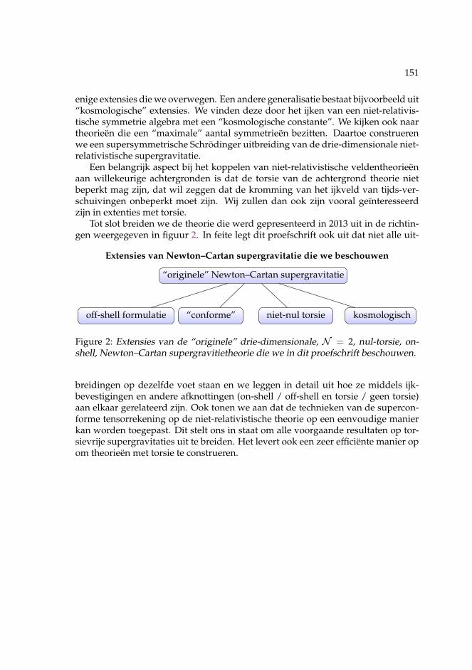
151
enige extensies die we overwegen. Een andere generalisatie bestaat bijvoorbeeld uit“kosmologische” extensies. We vinden deze door het ijken van een niet-relativis-tische symmetrie algebra met een “kosmologische constante”. We kijken ook naartheorieen die een “maximale” aantal symmetrieen bezitten. Daartoe construerenwe een supersymmetrische Schrodinger uitbreiding van de drie-dimensionale niet-relativistische supergravitatie.
Een belangrijk aspect bij het koppelen van niet-relativistische veldentheorieenaan willekeurige achtergronden is dat de torsie van de achtergrond theorie nietbeperkt mag zijn, dat wil zeggen dat de kromming van het ijkveld van tijds-ver-schuivingen onbeperkt moet zijn. Wij zullen dan ook zijn vooral geınteresseerdzijn in extenties met torsie.
Tot slot breiden we de theorie die werd gepresenteerd in 2013 uit in de richtin-gen weergegeven in figuur 2. In feite legt dit proefschrift ook uit dat niet alle uit-
Extensies van Newton–Cartan supergravitatie die we beschouwen
“originele” Newton–Cartan supergravitatie
off-shell formulatie “conforme” niet-nul torsie kosmologisch
Figure 2: Extensies van de “originele” drie-dimensionale, N = 2, nul-torsie, on-shell, Newton–Cartan supergravitietheorie die we in dit proefschrift beschouwen.
breidingen op dezelfde voet staan en we leggen in detail uit hoe ze middels ijk-bevestigingen en andere afknottingen (on-shell / off-shell en torsie / geen torsie)aan elkaar gerelateerd zijn. Ook tonen we aan dat de technieken van de supercon-forme tensorrekening op de niet-relativistische theorie op een eenvoudige manierkan worden toegepast. Dit stelt ons in staat om alle voorgaande resultaten op tor-sievrije supergravitaties uit te breiden. Het levert ook een zeer efficiente manier opom theorieen met torsie te construeren.

152
Acknowledgements
I can only agree with my colleagues who say that doing a PhD is not a lonely ven-ture. There are many people to whom I owe gratitude and I will try to mentioneveryone here. Let me start here in Groningen with the people I worked with andthen work my way geographically outwards.
First, let me start by thanking my supervisor Eric for his support throughout theyears, for his example in being a scientist and for his enthusiasm about science andphysics that motivated and helped me a lot in persisting while solving problemsthat proved to be difficult.
Ik wil ook graag de leden van mijn beoordelingscommissie Diederiek, Niels enStefan bedanken. Daarvoor dat jullie de tijd genomen hebben om honderdvijftigbladzijden over niet-relativistische zwaartekracht te lezen, ook omdat ik jullie hier-voor niet heel veel tijd heb gegeven door een vroege datum voor mijn verdedigingte kiezen.
I would also like to thank my paranymphs Stefan and Victor for taking on thisheavy burden and responsible task.
My work in Groningen was also facilitated by my colleagues and friends whowere helpful in giving scientific advice, answering my questions about physics,pretending to understand when I tried to explain something and more impor-tantly for providing distraction when my mind was too full of physics. Thankyou Aditya, Adolfo, Alasdair, Ana, Andrea, Andres, Blaise, Dennis, Diederiek,Dries, Giuseppe, Gokhan, Hanne, Hamid, Irene, Ivonne, Jan, Jan-Willem, Julian,Lorena, Luca, Lucia, Lucy, Marco, Marija, Mario, Pulastya, Remko, Roel,2 Shanka,Sjoerd, Souvik, Thiago, Victor, Wout and Yihao. Thanks are also due to Annelienand Iris for keeping the institute running, I hope that I did not cause you too muchtroubles.
With regards to my work I would also like to thank my “junior” collaboratorsLorena, Marija, Sjoerd, Wout and Yihao for our work and the related shared travel
154
experiences which included trips to many new countries. The advice and exam-ple of Eric, Daniel, Jan, Niklas and Quim have certainly helped me to become a(better) scientist.
I am grateful to Adolfo, Alessio, Andrea, Javier, Lorena and Sjoerd for joiningme in sportive activities such as football, tennis and running. More often thoughI was lazy and in this context I would like to thank Adolfo, Alasdair, Andrea,Andres, Giuseppe, Gokhan, Irene, Inge, Jan-Willem, Javier, Julian, Lorena, Lucy,Marija, Mario, Victor and Wout for the evenings watching football, playing poker,tasting Whiskey (or else) or (just?) watching South Park.
I also want to say thank you to my colleagues at other universities in the Nether-lands and people that I have met during schools and conferences. (Here, I willinevitably start to forget some names, but let me try nevertheless.) Thank you An-drea, Blaza, Celine, Daniel, Dennis, Ivano, Irfan, Joris, Laura, Natascia, Pablo,Paul, Ruben and Taeke for our physics discussions and perhaps some drinks.
Bij deze wil ik ook alle leden van de volleybal vereninging Kroton bedanken.Volleybal was altijd een fixpunt in mijn week, een zeer welkome afleiding en miss-chien ook mijn beste cursus Nederlands. Bovendien mocht ik met mijn team bin-nen drie jaar wel twee keer promoveren. In bijzonder gaat mijn dank dus uit naarmijn teamgenoten Alex, Alexei, Andrey, Daniel, Gerben, Jannes, Jøran, Lisanne,Matthijs, Roelof en Rutger maar ook naar alle anderen met wie ik nog mochttrainen: Anne, Christoph, Gerard, Iris,2 Josta, Jun, Lea, Leoni, Lin, Nine, Remco,Robbert, Rowan, Wen Hao en Yvonne.
Ich mochte mich auch nochmal separat bei meinem ersten Begleiter in Wienbedanken, der es mir erst ermoglicht hat die Stelle in Groningen zu finden undanzutreten. Vielen Dank Daniel, dass du es mir ermoglicht hast nach dem Erhaltmeines Diploms noch ein weiteres Jahr in Wien zu bleiben obwohl ich mich schonentschieden hatte eine PhD Stelle im Ausland zu suchen.
Dank gilt auch jenen Freunden in Wien, Alex, Bernhard, Fabian, Gerhard,Gregor, Joshy, Robert, Roman und Ulli, die mich warend meiner Aufenthaltedort durch Treffen, Fussball schauen, Schachspielen, Tarockieren, Borschodierenund/oder gemeinsame Urlaube meine Arbeit haben vergessen lassen.
Zum Schluss mochte ich mich noch bei meiner Familie bedanken. Meinen El-tern, Franz und Renate, dafur dass ihr mir nie Steine in den Weg gelegt habt, un-abhangig davon wie sehr ich euch vielleicht mit meinen beruflichen Entscheidun-gen uberrumpelt habe. Meinen Schwestern Lisi und Marlene, und den Familien,Emanuel, Johanna, Maria, Robert, Theresa (und Luna) dafur, dass ich in Arling-ton, Potomac, Wien und Wiener Neustadt immer willkommen war und Abwech-slung/Ablenkung von meiner Arbeit suchen durfte. Selbiges gilt naturlich auchfur meinen Bruder Stefan. Egal wie lang wir uns nicht gesehen haben, bei unserenTreffen kehrt immer binnen kurzester Zeit “Normalitat” ein. Wuck!
Thomas ZojerGroningen
December 2015
![Introduction to supergravity - arXiv · supersymmetry, but supergravity is introduced as well. The supergravity review [3] is still, 30 years later, a very good introduction. The](https://img.pdfslide.net/doc/110x75/5ec7a9f876d4fe3f047ef2a9/introduction-to-supergravity-arxiv-supersymmetry-but-supergravity-is-introduced.jpg)


![Non-relativistic supergravity in three space-time ...€¦ · curved backgrounds, see in particular [8–11] and [16]. These references together with [25–29] also point towards](https://img.pdfslide.net/doc/110x75/6021c4ce340b8c3b6466d783/non-relativistic-supergravity-in-three-space-time-curved-backgrounds-see-in.jpg)


![[Wess Bagger]Supersymmetry and Supergravity](https://img.pdfslide.net/doc/110x75/55cf8eb6550346703b94d652/wess-baggersupersymmetry-and-supergravity.jpg)