University of Jordan School of Engineering

Electrical Engineering Department

EE 219 Electrical Circuits Lab

EXPERIMENT 3 NETWORK THEOREMS

Prepared by: Dr. Mohammed Hawa

3-2

EXPERIMENT 3 NETWORK THEOREMS

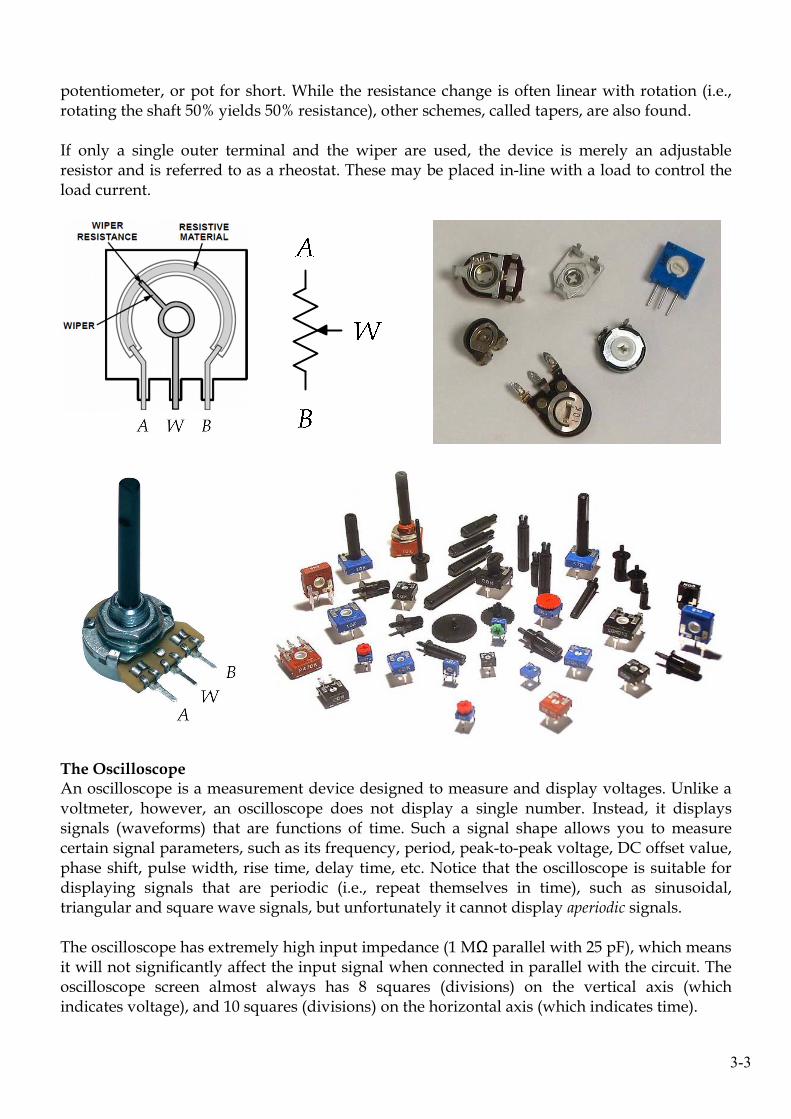
OBJECTIVE When you complete this experiment, you will have verified the superposition theorem as applied to multiple-source DC circuits. You will also have examined both the Thévenin and Norton theorems, the maximum power transfer condition, and learnt about the practical workings of adjustable resistances, namely the potentiometer and rheostat. Finally, you will have investigated the difference between peak-to-peak and rms values. DISCUSSION Superposition Theorem The superposition theorem states that in a linear multi-source AC or DC circuit, the current through (or voltage across) any particular element may be determined by considering the contribution of each source independently, with the remaining sources switched OFF (i.e., replaced with their internal resistances). The contributions are then summed, paying attention to polarities, to find the total value. Superposition cannot in general be applied to non-linear circuits or to non-linear quantities such as power. Thévenin and Norton Theorems Thévenin’s Theorem states that any linear circuit may be replaced by a single voltage source with an appropriate equivalent resistance. The Thévenin equivalent will produce the same load current and voltage as the original circuit to any load. The Thévenin voltage can be found by determining the open circuit output voltage. The Thévenin resistance is found by replacing sources with their internal resistances and determining the resulting combined resistance as seen from the two ports using standard series-parallel analysis techniques. In the laboratory, the Thévenin resistance may be found using an ohmmeter (again, when replacing the sources with their internal resistances); or by finding the open circuit voltage and short circuit current at the two desired ports. Norton’s theorem is the dual of Thévenin’s theorem, and states that any linear circuit may be replaced by an equivalent current source in parallel with an equivalent resistance. The equivalent current is the current obtained when short circuiting the two terminals in question. The equivalent resistance is the same as Thévenin’s equivalent resistance. Maximum Power Transfer In order to achieve the maximum load power in a circuit, the load resistance must equal the Thévenin resistance. Any load resistance value above or below this will produce a smaller load power. Potentiometer and Rheostat A potentiometer is a three terminal resistive device (see figure below). The outer terminals present a constant resistance which is the nominal value of the device. A third terminal, called the wiper arm, is a contact point that can be moved along the resistance. This three terminal configuration is used typically to adjust voltage via the voltage divider rule, hence the name

3-3

potentiometer, or pot for short. While the resistance change is often linear with rotation (i.e., rotating the shaft 50% yields 50% resistance), other schemes, called tapers, are also found. If only a single outer terminal and the wiper are used, the device is merely an adjustable resistor and is referred to as a rheostat. These may be placed in-line with a load to control the load current.

The Oscilloscope An oscilloscope is a measurement device designed to measure and display voltages. Unlike a voltmeter, however, an oscilloscope does not display a single number. Instead, it displays signals (waveforms) that are functions of time. Such a signal shape allows you to measure certain signal parameters, such as its frequency, period, peak-to-peak voltage, DC offset value, phase shift, pulse width, rise time, delay time, etc. Notice that the oscilloscope is suitable for displaying signals that are periodic (i.e., repeat themselves in time), such as sinusoidal, triangular and square wave signals, but unfortunately it cannot display aperiodic signals. The oscilloscope has extremely high input impedance (1 MΩ parallel with 25 pF), which means it will not significantly affect the input signal when connected in parallel with the circuit. The oscilloscope screen almost always has 8 squares (divisions) on the vertical axis (which indicates voltage), and 10 squares (divisions) on the horizontal axis (which indicates time).

3-4

The oscilloscope consists of five subsystems (see below): Horizontal controls, Vertical controls, Trigger controls, Quick measurement controls and Menu controls.

The main Horizontal controls are:

• Scale (Time-Per-Division): Determines the amount of time displayed.

• Position: Moves the waveform left and right (horizontally) on the display. The main Vertical controls are:

• Scale (Volts-Per-Division): Varies the size of the waveform on the screen.

• Position: Moves the waveform up and down (vertically) on the display.

• Input coupling: Determines which part of the signal is displayed as follows: - DC Coupling: Shows all of the input signal. - AC Coupling: Blocks the DC component of the signal, centering the waveform at 0 volts. - Ground Coupling: Disconnects the input signal to show where 0 volts is on the screen.

The main Trigger controls are:

• Source: Determines which signal is used for triggering the sweep.

• Level: Determines where on the edge of the source signal the trigger point occurs.

• Slope: Determines whether the trigger point is on the rising edge (positive slope) or the falling edge (negative slope) of the source signal.

The main Quick measurement controls are:

• Autoset: Adjusts horizontal, vertical and trigger settings automatically to display the input signals.

• Cursor: Places two horizontal or vertical lines (cursors) on top of the trace so the user can easily read values from the display.

• Measure: Automatically measures certain parameters from the screen (see Experiment 6).

3-5

PROCEDURE A – SUPERPOSITION THEOREM

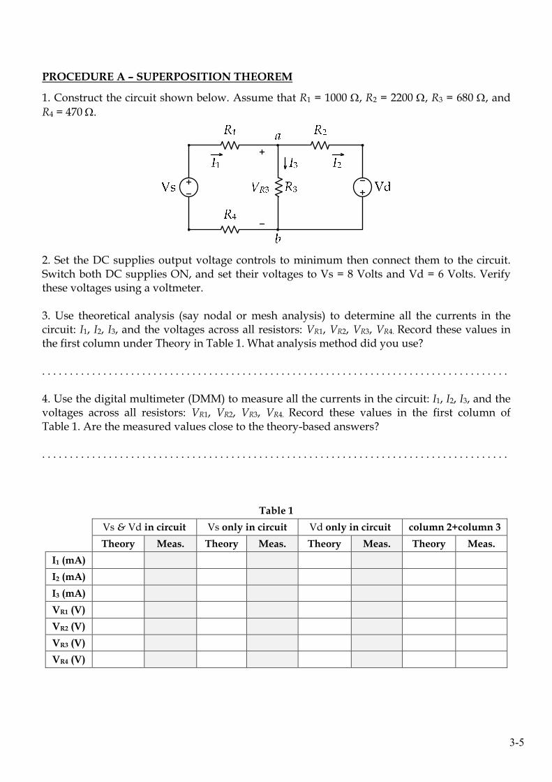
1. Construct the circuit shown below. Assume that R1 = 1000 Ω, R2 = 2200 Ω, R3 = 680 Ω, and

R4 = 470 Ω.

2. Set the DC supplies output voltage controls to minimum then connect them to the circuit. Switch both DC supplies ON, and set their voltages to Vs = 8 Volts and Vd = 6 Volts. Verify these voltages using a voltmeter. 3. Use theoretical analysis (say nodal or mesh analysis) to determine all the currents in the circuit: I1, I2, I3, and the voltages across all resistors: VR1, VR2, VR3, VR4. Record these values in the first column under Theory in Table 1. What analysis method did you use? . . . . . . . . . . . . . . . . . . . . . . . . . . . . . . . . . . . . . . . . . . . . . . . . . . . . . . . . . . . . . . . . . . . . . . . . . . . . . . . . . . . . 4. Use the digital multimeter (DMM) to measure all the currents in the circuit: I1, I2, I3, and the voltages across all resistors: VR1, VR2, VR3, VR4. Record these values in the first column of Table 1. Are the measured values close to the theory-based answers? . . . . . . . . . . . . . . . . . . . . . . . . . . . . . . . . . . . . . . . . . . . . . . . . . . . . . . . . . . . . . . . . . . . . . . . . . . . . . . . . . . . .

Table 1

Vs & Vd in circuit Vs only in circuit Vd only in circuit column 2+column 3

Theory Meas. Theory Meas. Theory Meas. Theory Meas.

I1 (mA)

I2 (mA)

I3 (mA)

VR1 (V)

VR2 (V)

VR3 (V)

VR4 (V)

3-6

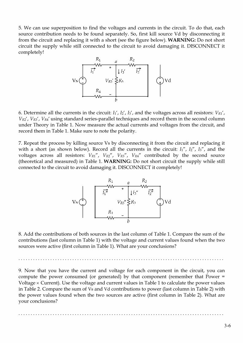
5. We can use superposition to find the voltages and currents in the circuit. To do that, each source contribution needs to be found separately. So, first kill source Vd by disconnecting it from the circuit and replacing it with a short (see the figure below). WARNING: Do not short circuit the supply while still connected to the circuit to avoid damaging it. DISCONNECT it completely!

6. Determine all the currents in the circuit: I1‘, I2‘, I3‘, and the voltages across all resistors: VR1‘, VR2‘, VR3‘, VR4‘ using standard series-parallel techniques and record them in the second column under Theory in Table 1. Now measure the actual currents and voltages from the circuit, and record them in Table 1. Make sure to note the polarity. 7. Repeat the process by killing source Vs by disconnecting it from the circuit and replacing it with a short (as shown below). Record all the currents in the circuit: I1”, I2”, I3”, and the voltages across all resistors: VR1”, VR2”, VR3”, VR4” contributed by the second source (theoretical and measured) in Table 1. WARNING: Do not short circuit the supply while still connected to the circuit to avoid damaging it. DISCONNECT it completely!

8. Add the contributions of both sources in the last column of Table 1. Compare the sum of the

contributions (last column in Table 1) with the voltage and current values found when the two sources were active (first column in Table 1). What are your conclusions? . . . . . . . . . . . . . . . . . . . . . . . . . . . . . . . . . . . . . . . . . . . . . . . . . . . . . . . . . . . . . . . . . . . . . . . . . . . . . . . . . . . . 9. Now that you have the current and voltage for each component in the circuit, you can compute the power consumed (or generated) by that component (remember that Power =

Voltage × Current). Use the voltage and current values in Table 1 to calculate the power values in Table 2. Compare the sum of Vs and Vd contributions to power (last column in Table 2) with the power values found when the two sources are active (first column in Table 2). What are your conclusions? . . . . . . . . . . . . . . . . . . . . . . . . . . . . . . . . . . . . . . . . . . . . . . . . . . . . . . . . . . . . . . . . . . . . . . . . . . . . . . . . . . . .

3-7

10. Is power a linear quantity or non-linear quantity? Why is this significant? . . . . . . . . . . . . . . . . . . . . . . . . . . . . . . . . . . . . . . . . . . . . . . . . . . . . . . . . . . . . . . . . . . . . . . . . . . . . . . . . . . . .

Table 2

Vs & Vd in circuit Vs only in circuit Vd only in circuit column 2+column 3

Theory Meas. Theory Meas. Theory Meas. Theory Meas.

PR1 (mW)

PR2 (mW)

PR3 (mW)

PR4 (mW)

PVs (mW)

PVd (mW)

11. What is the relationship between PR1 + PR2 + PR3 + PR4, on the one side, and PVs + PVd, on the other side? . . . . . . . . . . . . . . . . . . . . . . . . . . . . . . . . . . . . . . . . . . . . . . . . . . . . . . . . . . . . . . . . . . . . . . . . . . . . . . . . . . . . 12. When is it preferable to use superposition compared to nodal and mesh analysis? . . . . . . . . . . . . . . . . . . . . . . . . . . . . . . . . . . . . . . . . . . . . . . . . . . . . . . . . . . . . . . . . . . . . . . . . . . . . . . . . . . . . PROCEDURE B – THÉVENIN AND NORTON EQUIVALENT CIRCUITS

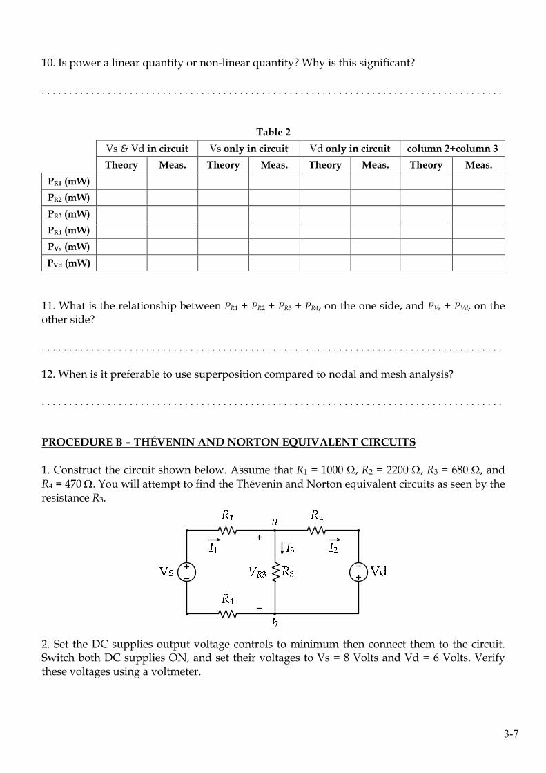
1. Construct the circuit shown below. Assume that R1 = 1000 Ω, R2 = 2200 Ω, R3 = 680 Ω, and

R4 = 470 Ω. You will attempt to find the Thévenin and Norton equivalent circuits as seen by the resistance R3.

2. Set the DC supplies output voltage controls to minimum then connect them to the circuit. Switch both DC supplies ON, and set their voltages to Vs = 8 Volts and Vd = 6 Volts. Verify these voltages using a voltmeter.

3-8

3. First, remove R3 to create an open circuit between terminals a and b as shown below. Evaluate the voltage VOC theoretically then measure it using a voltmeter. Pay attention to polarity. Record the values in the first column of Table 3.

4. Switch OFF the power supplies and replace the voltmeter with an ammeter between terminals a and b as shown below. Remember that the ammeter has a very small resistance, which mean it is almost a short circuit. WARNING: Be careful not to short circuit the power supplies using the ammeter.

5. Now switch ON the power supplies and measure the current ISC. Pay attention to polarity. Also evaluate the current ISC theoretically and record the values in the second column of Table 3. Then compute the value VOC/ISC.

Table 3

VOC (V) ISC (mA) VOC/ISC (Ω) Rab (Ω)

Theory Meas. Theory Meas. Theory Meas. Theory Meas.

6. Finally, kill both sources by disconnecting them from the circuit and replacing them with shorts. WARNING: Do not short circuit the supplies while still connected to the circuit to avoid damaging them. DISCONNECT them completely! 7. Remove the ammeter, and replace it with an Ohmmeter between terminals a and b. Record the Ohmmeter reading (Rab) in Table 3, along with the theoretical value. 8. Compare the values of VOC/ISC and Rab. State your conclusions. . . . . . . . . . . . . . . . . . . . . . . . . . . . . . . . . . . . . . . . . . . . . . . . . . . . . . . . . . . . . . . . . . . . . . . . . . . . . . . . . . . . .

3-9

9. Draw the theoretical Thévenin and Norton equivalent circuits for the above circuit with R3 connected. . . . . . . . . . . . . . . . . . . . . . . . . . . . . . . . . . . . . . . . . . . . . . . . . . . . . . . . . . . . . . . . . . . . . . . . . . . . . . . . . . . . . PROCEDURE C – MAXIMUM POWER TRANSFER

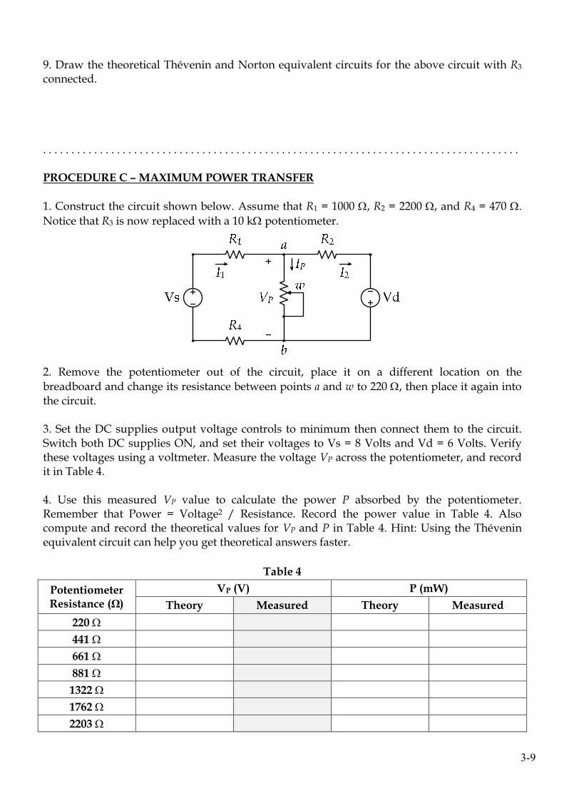
1. Construct the circuit shown below. Assume that R1 = 1000 Ω, R2 = 2200 Ω, and R4 = 470 Ω.

Notice that R3 is now replaced with a 10 kΩ potentiometer.

2. Remove the potentiometer out of the circuit, place it on a different location on the

breadboard and change its resistance between points a and w to 220 Ω, then place it again into the circuit. 3. Set the DC supplies output voltage controls to minimum then connect them to the circuit. Switch both DC supplies ON, and set their voltages to Vs = 8 Volts and Vd = 6 Volts. Verify these voltages using a voltmeter. Measure the voltage VP across the potentiometer, and record it in Table 4. 4. Use this measured VP value to calculate the power P absorbed by the potentiometer. Remember that Power = Voltage2 / Resistance. Record the power value in Table 4. Also compute and record the theoretical values for VP and P in Table 4. Hint: Using the Thévenin equivalent circuit can help you get theoretical answers faster.

Table 4

Potentiometer Resistance (Ω)

VP (V) P (mW)

Theory Measured Theory Measured

220 Ω

441 Ω

661 Ω

881 Ω

1322 Ω

1762 Ω

2203 Ω

3-10

5. Repeat the above process by disconnecting the potentiometer from the circuit, setting its resistance value to the ones shown in Table 4, placing it back into the circuit, and making the voltage measurements. 6. Why can’t you just measure the potentiometer resistance while it is still connected to the circuit?

. . . . . . . . . . . . . . . . . . . . . . . . . . . . . . . . . . . . . . . . . . . . . . . . . . . . . . . . . . . . . . . . . . . . . . . . . . . . . . . . . . . . 7. Plot the absorbed power P versus potentiometer resistance (provide handwritten plots on the graph paper attached at the end of the report). At what resistance value do you observe maximum power transfer?

. . . . . . . . . . . . . . . . . . . . . . . . . . . . . . . . . . . . . . . . . . . . . . . . . . . . . . . . . . . . . . . . . . . . . . . . . . . . . . . . . . . . 8. What is so special about the above resistance value? Hint: review procedure B.

. . . . . . . . . . . . . . . . . . . . . . . . . . . . . . . . . . . . . . . . . . . . . . . . . . . . . . . . . . . . . . . . . . . . . . . . . . . . . . . . . . . . PROCEDURE D – PEAK-TO-PEAK VERSUS RMS VALUES

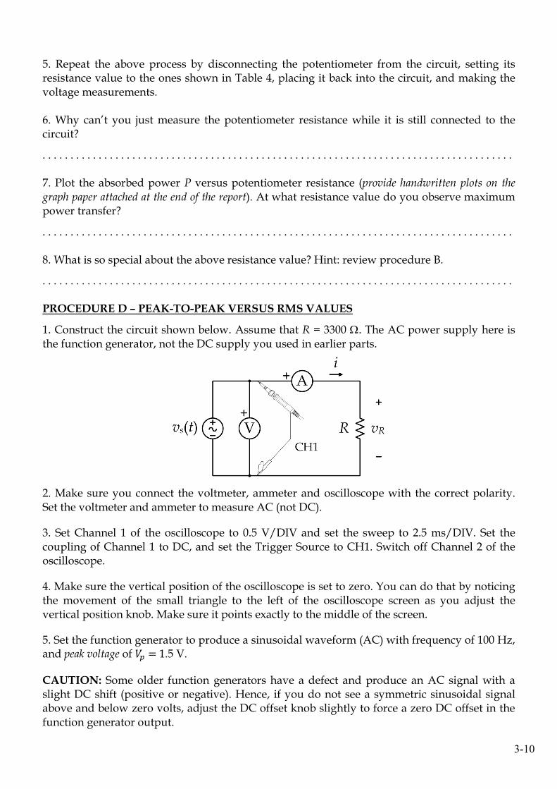
1. Construct the circuit shown below. Assume that R = 3300 Ω. The AC power supply here is the function generator, not the DC supply you used in earlier parts.

2. Make sure you connect the voltmeter, ammeter and oscilloscope with the correct polarity. Set the voltmeter and ammeter to measure AC (not DC).

3. Set Channel 1 of the oscilloscope to 0.5 V/DIV and set the sweep to 2.5 ms/DIV. Set the coupling of Channel 1 to DC, and set the Trigger Source to CH1. Switch off Channel 2 of the oscilloscope.

4. Make sure the vertical position of the oscilloscope is set to zero. You can do that by noticing the movement of the small triangle to the left of the oscilloscope screen as you adjust the vertical position knob. Make sure it points exactly to the middle of the screen.

5. Set the function generator to produce a sinusoidal waveform (AC) with frequency of 100 Hz, and peak voltage of 1.5 V.

CAUTION: Some older function generators have a defect and produce an AC signal with a slight DC shift (positive or negative). Hence, if you do not see a symmetric sinusoidal signal above and below zero volts, adjust the DC offset knob slightly to force a zero DC offset in the function generator output.

3-11

6. What is the period (in milliseconds) of the sinusoidal signal out of the function generator?

. . . . . . . . . . . . . . . . . . . . . . . . . . . . . . . . . . . . . . . . . . . . . . . . . . . . . . . . . . . . . . . . . . . . . . . . . . . . . . . . . . . . 7. Draw what you see on the oscilloscope screen below. Make sure you have Channel 1 of the oscilloscope set to 0.5 V/DIV and the sweep set to 2.5 ms/DIV.

8. Use theoretical analysis to determine the rms value of the source voltage () and the current in the circuit () at the different frequencies shown in Table 5. Record these values in the table? What equation should you use to calculate the current in rms from the peak source voltage ?

. . . . . . . . . . . . . . . . . . . . . . . . . . . . . . . . . . . . . . . . . . . . . . . . . . . . . . . . . . . . . . . . . . . . . . . . . . . . . . . . . . . . 9. Measure the peak-to-peak value of the source voltage using the oscilloscope screen at

the different frequencies and record them in the first column of Table 5. CAUTION: Whenever you change the frequency of the function generator, verify the period of the signal from the oscilloscope. Also re-check the peak-to-peak voltage as the function generator might change the amplitude when you change the frequency.

Table 5

AC Source Frequency

(Hz)

Source (V) (Oscilloscope)

Source (V) (Oscilloscope)

Source (V) (Voltmeter)

(mA) (Ammeter)

Theory Meas. Theory Meas. Theory Meas. Theory Meas.

100

1000

2000

3-12

10. Evaluate the measured rms value of the source voltage using the peak-to-peak oscilloscope reading, and record this in the second column of Table 5. 11. Now use the voltmeter to read the measured rms value of the source voltage, but record the answer this time in the third column of Table 5. How are the voltmeter and oscilloscope different in reading the AC voltage? . . . . . . . . . . . . . . . . . . . . . . . . . . . . . . . . . . . . . . . . . . . . . . . . . . . . . . . . . . . . . . . . . . . . . . . . . . . . . . . . . . . . 12. What extra information about the source voltage can the oscilloscope provide, which the voltmeter cannot provide? . . . . . . . . . . . . . . . . . . . . . . . . . . . . . . . . . . . . . . . . . . . . . . . . . . . . . . . . . . . . . . . . . . . . . . . . . . . . . . . . . . . . 13. Use the ammeter to measure the rms value of the current, and record the answer in the last column of Table 5. Are the measurements close to the theoretical answers? . . . . . . . . . . . . . . . . . . . . . . . . . . . . . . . . . . . . . . . . . . . . . . . . . . . . . . . . . . . . . . . . . . . . . . . . . . . . . . . . . . . . 14. Does the resistor change its impedance ZR with frequency? . . . . . . . . . . . . . . . . . . . . . . . . . . . . . . . . . . . . . . . . . . . . . . . . . . . . . . . . . . . . . . . . . . . . . . . . . . . . . . . . . . . . 15. What if you only had an oscilloscope without an ammeter. How would you be able to measure the current in the circuit in rms? Explain clearly. . . . . . . . . . . . . . . . . . . . . . . . . . . . . . . . . . . . . . . . . . . . . . . . . . . . . . . . . . . . . . . . . . . . . . . . . . . . . . . . . . . . .

** End **