UNIVERSITY OF NAIROBI SCHOOL OF ENGINEERING

DEPARTMENT OF ENVIRONMENTAL AND BIOSYSTEMS ENGINEERING

DESIGN OF A SLAUGHTERHOUSE WASTEWATER TREATMENT SYSTEM:

CASE STUDY OF BAHATI SLAUGHTERHOUSE LIMURU TOWN

CANDIDATE NAME: RONO BERNARD KIPSANG

CANDIDATE No.: F21/36666/2010

SUPERVISOR’S NAME: DR OMUTO CHRISTIAN THINE

A Report Submitted in Partial Fulfillment for the Requirements of the Degree of Bachelor of Science in Environmental and Biosystems Engineering, of the University Of Nairobi

29th MAY, 2015

FEB 540: ENGINEERING DESIGN PROJECT

2014/2015 ACADEMIC YEAR

i | P a g e F 2 1 / 3 6 6 6 6 / 2 0 1 0

DECLARATION

I declare that this project, except where specifically acknowledged, is my original work. This

report has not been in whole or in part submitted for any degree or examination at any other

University.

Rono Bernard Kipsang

Signature………………………. Date…………………………..

This project report has been submitted for examination with my approval as University

Supervisor

Dr. Omuto Christian Thine

Signature………………………. Date…………………………..

ii | P a g e F 2 1 / 3 6 6 6 6 / 2 0 1 0

DEDICATION

I dedicate this Project to my dad, Dr. David Lagat, mum, Mrs. Rael Lagat, and my four beloved

sisters, Josephine, Naomy, Nancy and Caroline and to all my dear friends.

You guys are the source of my strength and drive to push on.

iii | P a g e F 2 1 / 3 6 6 6 6 / 2 0 1 0

ACKNOWLEDGEMENT

I am grateful to God Almighty for the strength throughout the five years I have been at the

University.

I would like to sincerely thank my supervisor Dr. Omuto Christian Thine for his guidance and

support throughout my design project. Without his assistance, ability to come up with this design

project would not have been possible.

My immense gratitude also goes to Dr. Isaac Alukwe whose contribution came in handy during

the inception stage of this project. His contribution was also very vital in developing the concept

note and the proposal and also for his valuable comments on the draft text.

Special thanks to Mr. B.A. Muliro and Ann Rose (Soil Lab Team), Joyce Wambui (Public

Health Engineering Lab Technician) for their great guidance in soil and wastewater analysis

respectively. Deep appreciation to the Bahati slaughterhouse management for granting access to

their premises and giving relevant information about the waste management system used in the

past.

This design project report would not have been realized without the support of my family, whose

love and encouragement has always given me the confidence to believe in my own abilities.

Above all, though, I would like to thank Daisy and Ethan, who quite simply means the world to

me. This design project report is dedicated to them.

To all those who contributed, my deepest gratitude

iv | P a g e F 2 1 / 3 6 6 6 6 / 2 0 1 0

ABSTRACT

Due to the imposition of strict limits of wastewater discharges and the possibility of water reuse,

there is a greater demand to treat wastewater efficiently. The objective of this design project is to

come up with a slaughterhouse wastewater treatment system for the treatment of Bahati

slaughterhouse wastewater that meets the effluent quality standards before discharge.

The proposed system is composed of an Anaerobic Sequencing Batch Reactor (ASBR). This is a

new generation of a high rate anaerobic treatment system, it has a high efficiency at higher

loading rates and is applicable for extreme environmental conditions and to inhibitory

compounds.

Wastewater Samples and soil samples were collected. Wastewater content were determined

through lab tests and used to analyze the quantity and composition of slaughterhouse wastewater.

The results are shown in Table 4.1. Geotechnical data and analysis was carried out using triaxial

compression test. The strength parameters of the soil were determined and results shown in table

4.3.

The design was done for two ASBR basins each with a flow capacity of 16.68 m3/day. The Basin

working volume of the ASBR was found to be 30.68 m3.The dimensions of the ASBR were

found to be 3300 mm in diameter, a total height of 5570 mm and section thickness of 300 mm.

The decanter size was obtained to be 300 mm with a decanter rate of 127.38 l/min during peak

hour. Hydraulic Retention Time was determined to be 2.78days while the Mean Residence Time

is 19.45 days.

The ASBR incorporates a blower with a Blower Unit Capacity of 11.29 m3/min, Blower pressure

of 146.42 Kpa and maximum blower brake horse power of 3.11 Hp. This will be sufficient to

provide a standard oxygen required of 34.64 kg/basin/day and can also achieve a maximum

aeration depth of 3910 mm. A multistage mechanical agitator with pitched 3-blade turbine is

incorporated at the center of the ASBR basin for dissolving solids and dispersing a gas in the liquid.

The structural design of the ASBR was achieved by determining the crack analysis using the BS

8007 code of practice. The crack width of 0.04 was obtained and since this crack width is less

than 0.1, the appearance and durability of the structural element were not affected since this is

within the limits of crack width as specified by IS: 1343-1980.

The top cover of the ASBR was designed to have a fixed dome shape that is air tight so as

increase the pressure of the biogas in the reactor hence allowing the collection of daily gas

production that was calculated to be 1.47 m3/basin/day. The cover has a provision for biogas line,

a mechanical agitator, pH dosing line and an access point of sufficient size (600 mm by 900 mm)

for inspection, cleaning and testing.

The objectives of the design were met and this design project report shows a complete design of

a wastewater treatment plant. It is, however, important to apply the following recommendations

to the treatment system in order to optimize it to improve its performance. This include;

increasing the diameter of the basin, this helps to increase the basin area and thus reducing the

overall depth; Reducing the amount of water used for general cleaning purposes and to improve

the quality of the ASBR-treated effluent, aerobic post treatment should be introduced to further

remove suspended solids, organic and nutrients like nitrogen and phosphorus

v | P a g e F 2 1 / 3 6 6 6 6 / 2 0 1 0

List of Tables

Table 2.1 Typical operating conditions of various AD configurations ........................................ 19

Table 2.2 Different available technologies used to treat slaughterhouse wastewater. .................. 20

Table 4.1 Composition of slaughterhouse wastewater ................................................................. 32

Table 4.2 Time operation for every cycle ..................................................................................... 34

Table 4.3 Strength Parameters of the Soil .................................................................................... 47

Table 4.4 Structural design parameters for concrete structure ..................................................... 49

Table 9.1 Data for specimen A1, profile layer (0-30) cm ............................................................. 69

Table 9.2 Data for specimen A2, profile layer (0-30) cm ............................................................. 70

Table 9.3 Data for specimen A3, profile layer (0-30) cm ............................................................. 71

Table 9.4 Data for specimen B1, profile layer (30-60) cm............................................................ 75

Table 9.5 Data for specimen B2, profile layer (30-60) cm............................................................ 76

Table 9.6 Data for specimen B3, profile layer (30-60) cm............................................................ 77

Table 9.7 Data for specimen C1, profile layer (60-90) cm............................................................ 80

Table 9.8 Data for specimen C2, profile layer (60-90) cm............................................................ 81

Table 9.9 Data for specimen C3, profile layer (60-90) cm............................................................ 82

vi | P a g e F 2 1 / 3 6 6 6 6 / 2 0 1 0

Table of Figures

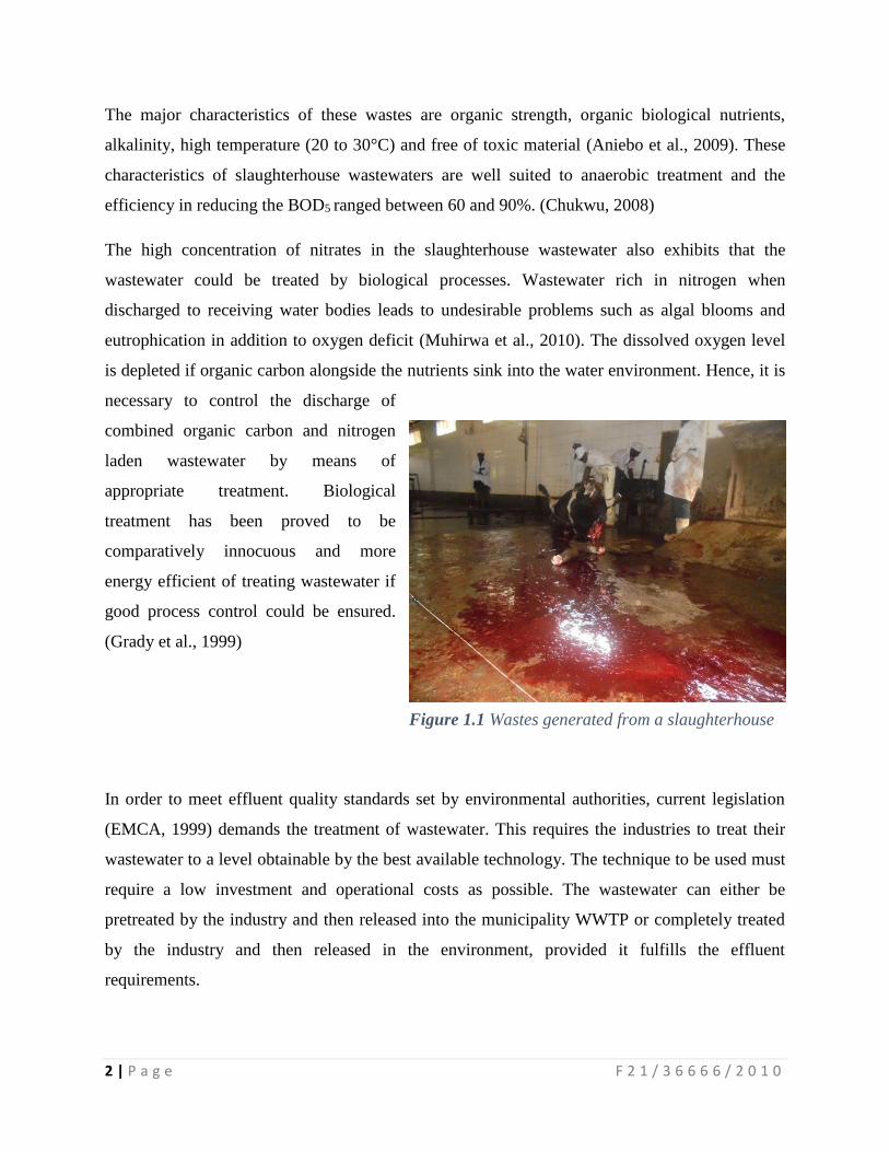
Figure 1.1 Wastes generated from a slaughterhouse ...................................................................... 2

Figure 1.2 Study area map .............................................................................................................. 5

Figure 1.3 Study location map for Bahati slaughterhouse using QGIS 2.4.0 ................................. 6

Figure 2.1 Simplified process flow diagram for a typical large-scale treatment plant. ................ 10

Figure 2.2 The electron tower ....................................................................................................... 11

Figure 2.3 Metabolic microbial groups involved in anaerobic waste water treatment process .... 12

Figure 2.4 Fermentation process ................................................................................................... 13

Figure 2.5 Difference between methanogenesis and acetogenesis ............................................... 15

Figure 2.6 Reactions involved in and nature of interspecies hydrogen transfer ........................... 16

Figure 2.7 Different phases of a batch reactor in one operating cycle ......................................... 23

Figure 2.8 A schematic diagram of the experimental setup .......................................................... 25

Figure 4.1 Circular reservoir configuration .................................................................................. 48

Figure 4.2 Layouts of multi-stage agitator and pitched 3-blade turbine with pitch angle 450 ...... 54

Figure 9.1 Source of waste inform of blood as a result of slaughtering ....................................... 63

Figure 9.2 Floor showing waste generated during slaughtering ................................................... 63

Figure 9.3 Waste collection generated from the processing of the red offals ............................... 64

Figure 9.4 Processing of the white offals on the floor .................................................................. 64

Figure 9.5 Mixture of blood, urine and digested wastes ............................................................... 65

Figure 9.6 Wastewater from the processing of the white ovals .................................................... 65

Figure 9.7 Effluent entering into the wetland ............................................................................... 66

Figure 9.8 The polluted Manguo wetland ..................................................................................... 66

Figure 9.9 Graph of unit axial load against axial strain, profile layer 0 - 30 cm .......................... 72

Figure 9.10 Mohr circle diagram for profile layer 0-30 cm .......................................................... 73

Figure 9.11 Graph of unit axial load against axial strain, profile layer 30 – 60 cm ..................... 77

Figure 9.12 Mohr circle diagram for profile layer 30 - 60 cm ...................................................... 78

Figure 9.13 Graph of unit axial load against axial strain, profile layer 60 – 90 cm ..................... 83

Figure 9.14 Mohr circle diagram for profile layer 60 - 90 cm ...................................................... 84

Figure 9.15 An isometric view of an ASBR ................................................................................. 88

Figure 9.16 Two dimensional drawing of an ASBR basin ........................................................... 89

Figure 9.17 Layout of a multi-stage agitator ................................................................................ 90

Figure 9.18 Layout of an impeller ................................................................................................ 91

Figure 9.19 Dual train layout of the ASBR basins (front view 3D) ............................................. 92

Figure 9.20 Dual train layout of the basis ..................................................................................... 93

vii | P a g e F 2 1 / 3 6 6 6 6 / 2 0 1 0

List of acronyms and abbreviations

ABR: Anaerobic Baffled Reactor

ACP: Anaerobic Contact Process

ACR: Anaerobic Contact Reactor

ADP: Adenosine Di-phosphate

ASBR: Anaerobic Sequencing Batch Reactor

ATP: Adenosine Tri-phosphate

BOD, BOD5: 5-Day Biochemical Oxygen Demand

BUC: Blower Unit Capacity

CAS: Conventional Activated Sludge

C/B: Cost Benefit Ratio

COD: Chemical Oxygen Demand

EGSB: Expanded Granular Sludge Bed

EMCA: Environmental Management and Co-ordination Act

GHP: Good Hygiene Practices

GMP: Good Manufacturing Practices

HRT: Hydraulic Retention Time

KARI: Kenya Agricultural Research Institute

MPSA: Multi-Phase Staged Anaerobic

NEMA: National Environmental Management Authority

NNFCC: National Non-Food Crops Centre

OLR: Organic Loading Rates

RAS: Returned Activated Sludge

STR: Solid Retention Time

TSS: Total Suspended Solids

UASB: Upflow Anaerobic Sludge Blanket

WWTP: Waste Water Treatment Plant

viii | P a g e F 2 1 / 3 6 6 6 6 / 2 0 1 0

Table of Contents

1 INTRODUCTION ................................................................................................................... 1

1.1 Background ...................................................................................................................... 1

1.2 Statement of the Problem and Problem Analysis ............................................................. 3

1.3 Site Analysis and Inventory ............................................................................................. 4

1.3.1 Description of the project Location .......................................................................... 4

1.3.2 Mapping the study area ............................................................................................. 5

1.3.3 Climate ...................................................................................................................... 7

1.3.4 Geology ..................................................................................................................... 7

1.3.5 Land use .................................................................................................................... 7

1.4 Objectives ......................................................................................................................... 8

1.4.1 The broad objective................................................................................................... 8

1.4.2 Specific objectives .................................................................................................... 8

1.5 Statement of Scope ........................................................................................................... 8

2 LITERATURE REVIEW AND THEORETICAL FRAMEWORK ....................................... 9

2.1 Literature review .............................................................................................................. 9

2.1.1 Treatment process ..................................................................................................... 9

2.1.2 Anaerobic process for waste water treatment ......................................................... 10

2.1.3 Advantages and disadvantages of anaerobic process .............................................. 16

2.1.4 Common applications of anaerobic process ........................................................... 18

2.1.5 Applicability of anaerobic process for slaughterhouse wastewater ........................ 19

2.1.6 Anaerobic Sequencing Batch Reactor (ASBR) ...................................................... 22

2.2 Theoretical Framework .................................................................................................. 26

2.2.1 Biochemical Oxygen Demand (BOD) .................................................................... 26

2.2.2 Chemical Oxygen Demand (COD) ......................................................................... 27

2.2.3 Total Suspended Solids (TSS) ................................................................................ 28

2.2.4 Flow rate (Q)/ daily wastewater generation ............................................................ 28

2.2.5 Volume of the reactor ............................................................................................. 28

2.2.6 Solid Retention Time (SRT or Θx) ......................................................................... 29

2.2.7 Hydraulic Retention Time (HRT), .......................................................................... 29

3 GENERATION OF CONCEPT DESIGN ............................................................................ 30

3.1 Description of the design project methodology ............................................................. 30

3.2 Data Collection ............................................................................................................... 30

3.3 Location of the project ................................................................................................... 30

ix | P a g e F 2 1 / 3 6 6 6 6 / 2 0 1 0

3.4 Data collected and its uses to address objectives ........................................................... 31

3.5 Analysis of the data obtained. ........................................................................................ 31

3.6 Modelling the system/making design drawings ............................................................. 31

4 RESULTS AND DATA ANALYSIS ................................................................................... 32

4.1 Raw Slaughterhouse Wastewater Data .......................................................................... 32

4.2 Flow rate estimates/daily wastewater production .......................................................... 32

4.3 Design parameters .......................................................................................................... 33

4.3.1 Influent conditions .................................................................................................. 33

4.3.2 Effluent conditions .................................................................................................. 33

4.3.3 Process design criteria............................................................................................. 34

4.4 Design Calculations (BOD Removal and Nitrification Process) ................................... 34

4.4.1 BOD load (BODL) .................................................................................................. 34

4.4.2 Mass of Biomass for BOD Removal ...................................................................... 34

4.4.3 Nitrogen Load ......................................................................................................... 35

4.4.4 Mass of Biomass Required for Nitrification ........................................................... 35

4.4.5 Design Mass of Biomass ......................................................................................... 35

4.4.6 Volume of Biomass................................................................................................. 36

4.4.7 Maximum volume above bottom water level ......................................................... 36

4.4.8 Decant Rates ........................................................................................................... 37

4.4.9 Decanter Sizing ....................................................................................................... 37

4.4.10 Basin Working Volume .......................................................................................... 38

4.4.11 Basin Area ............................................................................................................... 38

4.4.12 Sludge Depth ........................................................................................................... 38

4.4.13 Decanter Draw Down ............................................................................................. 39

4.4.14 Bottom Water Level ................................................................................................ 39

4.4.15 Top Water Level ..................................................................................................... 39

4.4.16 Hydraulic Retention Time ....................................................................................... 39

4.4.17 MLSS Concentration at Bottom Water Level ......................................................... 40

4.4.18 Mass of Sludge Produced........................................................................................ 40

4.4.19 Volume of Sludge Produced ................................................................................... 40

4.4.20 Mean Cell Residence Time ..................................................................................... 41

4.4.21 Waste Sludge Pump Capacity ................................................................................. 41

4.5 Air calculations (BOD Removal and Nitrification Process) .......................................... 42

4.5.1 Actual oxygen required ........................................................................................... 42

x | P a g e F 2 1 / 3 6 6 6 6 / 2 0 1 0

4.5.2 Standard Oxygen Requirement ............................................................................... 43

4.5.3 Maximum Aeration Depth ...................................................................................... 44

4.5.4 Air Flow Requirement ............................................................................................ 45

4.5.5 Blower Unit Capacity ............................................................................................. 46

4.5.6 Blower Pressure ...................................................................................................... 46

4.5.7 Maximum Blower Brake Horse Power ................................................................... 46

4.6 Daily gas production rate ............................................................................................... 46

4.7 Geotechnical Data and Analysis .................................................................................... 47

4.8 Structural design of concrete structure for retaining the wastewater ............................. 48

4.8.1 Determining crack analysis using BS 8007 code of practice. ................................. 48

4.8.2 Provision for access ................................................................................................ 54

4.9 Design layout of a mechanical agitator .......................................................................... 54

4.9.1 Geometrical parameters of multi-stage agitator ...................................................... 55

5 DISCUSSION ........................................................................................................................ 56

6 CONCLUSION ..................................................................................................................... 58

7 RECOMMENDATIONS....................................................................................................... 59

8 REFERENCES ...................................................................................................................... 60

9 APPENDICES ....................................................................................................................... 63

9.1 Appendix A: Site Photographs ....................................................................................... 63

9.2 Appendix B: Standard for discharge into natural water courses .................................... 67

9.3 Appendix C: Triaxial compression test .......................................................................... 69

9.3.1 Results ..................................................................................................................... 69

9.4 Appendix D: BS 8007 code of practice .......................................................................... 86

9.4.1 Calculation of crack widths in mature concrete ...................................................... 86

9.5 Appendix E: Areas of groups of reinforcement bars (mm2) .......................................... 87

9.6 Design drawings ............................................................................................................. 88

1 | P a g e F 2 1 / 3 6 6 6 6 / 2 0 1 0

1 INTRODUCTION

1.1 Background

Meat processing has grown to become one of the integral components of every economy. This is

due to the continuous drive to increase meat production essential for meeting the protein needs of

the ever increasing world population. The establishment of Slaughterhouses and processing

plants is on the rise. Owing to the intensive nature of meat processing, effluents from such plants

contain pollutants. Discharging these pollutants into the environment in their raw state is

hazardous. Pollution arises from activities that fail to adhere to Good Manufacturing Practices

(GMP) and Good Hygiene Practices (GHP) (Akinro et al., 2009)

For hygienic reasons, large amount of water is used in meat processing operations (slaughtering

and cleaning), which produces wastewater. The major environmental problem associated with

slaughterhouse wastewater is the large amount of suspended solids and liquid waste as well as

odor generation. (Gauri, 2006)

The wastewater is rich in fats, protein and cellulose, and often has a low Carbon-to-Nitrogen

ratio (Linda, 2005). Effluent from slaughterhouses has also been recognized to contaminate both

surface and groundwater because during abattoir processing; blood, fat, manure, urine, and meat

tissues are lost to the wastewater streams (Bello and Oyedemi, 2009). Leaching into ground

water is a major part of the concern, especially due to the recalcitrant nature of some

contaminants. (Muhirwa et al., 2010)

Blood, one of the major dissolved pollutants in abattoir wastewater, has the highest COD of any

effluent from abattoir operations. If the blood from a single cow carcass is allowed to discharge

directly into a sewer line, the effluent load would be equivalent to the total sewage produced by

50 people on average day. (Aniebo et al., 2009)

The waste from slaughterhouse is estimated to contain; approx. 1,000 to 4,000 mg/L BOD,

approx. 2,000 to 10,000 mg/L COD, approx. 200 to 1,500 mg/L SS, High Oil and Grease

content, possible high chloride content from salting skins (Lawrence, 2006).

2 | P a g e F 2 1 / 3 6 6 6 6 / 2 0 1 0

The major characteristics of these wastes are organic strength, organic biological nutrients,

alkalinity, high temperature (20 to 30°C) and free of toxic material (Aniebo et al., 2009). These

characteristics of slaughterhouse wastewaters are well suited to anaerobic treatment and the

efficiency in reducing the BOD5 ranged between 60 and 90%. (Chukwu, 2008)

The high concentration of nitrates in the slaughterhouse wastewater also exhibits that the

wastewater could be treated by biological processes. Wastewater rich in nitrogen when

discharged to receiving water bodies leads to undesirable problems such as algal blooms and

eutrophication in addition to oxygen deficit (Muhirwa et al., 2010). The dissolved oxygen level

is depleted if organic carbon alongside the nutrients sink into the water environment. Hence, it is

necessary to control the discharge of

combined organic carbon and nitrogen

laden wastewater by means of

appropriate treatment. Biological

treatment has been proved to be

comparatively innocuous and more

energy efficient of treating wastewater if

good process control could be ensured.

(Grady et al., 1999)

In order to meet effluent quality standards set by environmental authorities, current legislation

(EMCA, 1999) demands the treatment of wastewater. This requires the industries to treat their

wastewater to a level obtainable by the best available technology. The technique to be used must

require a low investment and operational costs as possible. The wastewater can either be

pretreated by the industry and then released into the municipality WWTP or completely treated

by the industry and then released in the environment, provided it fulfills the effluent

requirements.

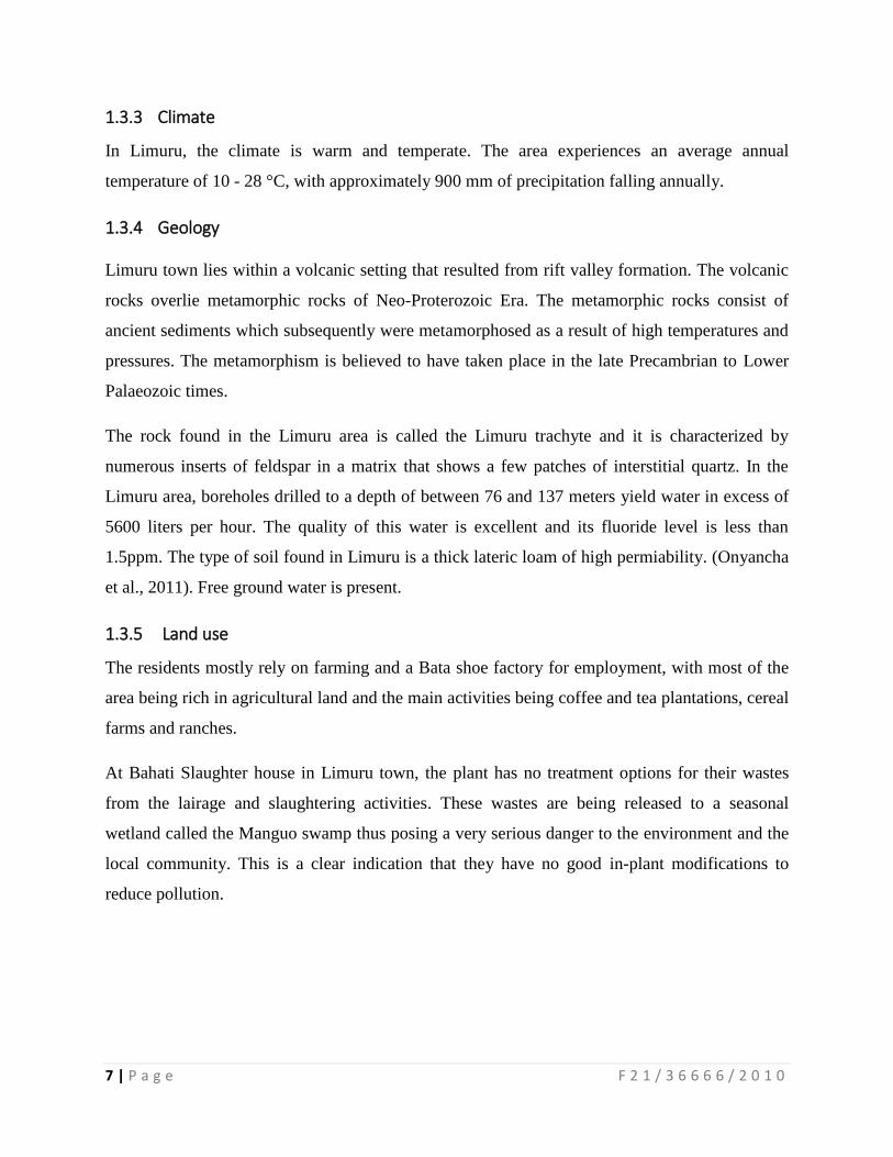
Figure 1.1 Wastes generated from a slaughterhouse

3 | P a g e F 2 1 / 3 6 6 6 6 / 2 0 1 0

1.2 Statement of the Problem and Problem Analysis

Bahati slaughterhouse drains its wastewater direct to the Manguo seasonal swamp and

eventually, this wastewater flows into the waterways. Wastewater generated from

slaughterhouses, occur in form of bulking sludge which contains diluted blood, protein, fat, and

suspended solids. As a result, the organic and nutrient concentration in this wastewater is very

high and the residues are partially solubilized, leading to a highly contaminating effect in

riverbeds and other water bodies. This poses a threat to both the area residents and aquatic

organisms. These wastes also decompose to form methane, carbon dioxide and odor causing air

pollution. (Grady et al., 1999)

The slaughterhouse wastewater originates from two different sources. The first source is the

temporary holding pen and the other source is from the slaughter area. Slaughterhouse

wastewater is a largest contributor to toxic pollution in waterbodies. Some of the issues that lead

to pollution from these wastes include; Biochemical Oxygen Demand (BOD), Chemical Oxygen

Demand (COD), nitrate, phosphates, and potassium. The presence of high BOD may indicate

fecal contamination or increases in particulate and dissolved organic carbon from animal sources

that can restrict water use and development.

Increased oxygen consumption poses a potential threat to a variety of aquatic organisms. Organic

pollution can occur when inorganic pollutants such as nitrogen and phosphates accumulate in

aquatic ecosystems. High levels of these nutrients cause an overgrowth of plants and algae and

this eventually leads to eutrophication and anoxia.

This organic pollution alters the aquatic ecosystem and makes the water unfit for consumption.

Runoff during heavy rainfalls from the natural wetland contaminates nearby water sources,

leaching may contaminate groundwater and pose a health risk due to disease causing bacteria and

pathogens. Thus the best treatment option is to set up an on-site wastewater treatment

mechanism before discharging the wastes to the environment. This project will involve the

design of a suitable anaerobic reactor technology for wastewater treatment.

4 | P a g e F 2 1 / 3 6 6 6 6 / 2 0 1 0

1.3 Site Analysis and Inventory

1.3.1 Description of the project Location

Limuru is a town in Central Kenya, Kiambu County with a population of about 8,985 as of 2015.

It is located on the eastern edge of the Great Rift Valley about 40 kilometers North-West

from Nairobi. Altitude of the town is about 2,500 meters with a latitude 10 06’ 00’’ S, longitude

360 39’ 00” E.

Meat processing at the Bahati slaughter house is located on plot LR No 811 and occupies 0.82

hectares (2.026 acres) and the slaughterhouse is located 35km from Nairobi just off the Nairobi –

Nakuru highway at Limuru.

The slaughterhouse is set on a gentle sloping piece of land which borders a seasonal wetland

called the Manguo swamp which hosts several species of flora and fauna. Mud fishes have been

seen at this swamp.

The activity carried out at the slaughterhouse is the slaughtering of beef cattle and sheep, which

are supplied by pastoral community and the local residents. The meat is then bought by meat

buyers from the nearby areas of Limuru, Kiambu, Kabuki, Tigoni and Nairobi.

The slaughter house has the following facilities: holding pens, stunning box, killing and dressing

line, hides and skins processing area, blood recovery tank, red offals processing area, white

offals processing area, inspection and grading area, loading bay, changing room, ablution block,

offices, and tanks for holding wastes.

The installed capacity is 100 beef cattle and 30 sheep per day. The slaughterhouse is serviced

with electricity, borehole water and tarmacked road.

5 | P a g e F 2 1 / 3 6 6 6 6 / 2 0 1 0

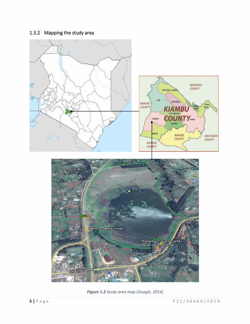
1.3.2 Mapping the study area

Figure 1.2 Study area map (Google, 2014)

6 | P a g e F 2 1 / 3 6 6 6 6 / 2 0 1 0

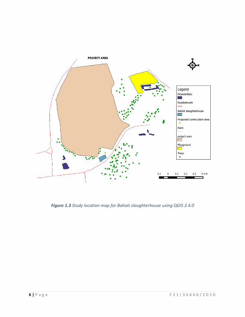
Figure 1.3 Study location map for Bahati slaughterhouse using QGIS 2.4.0

7 | P a g e F 2 1 / 3 6 6 6 6 / 2 0 1 0

1.3.3 Climate

In Limuru, the climate is warm and temperate. The area experiences an average annual

temperature of 10 - 28 °C, with approximately 900 mm of precipitation falling annually.

1.3.4 Geology

Limuru town lies within a volcanic setting that resulted from rift valley formation. The volcanic

rocks overlie metamorphic rocks of Neo-Proterozoic Era. The metamorphic rocks consist of

ancient sediments which subsequently were metamorphosed as a result of high temperatures and

pressures. The metamorphism is believed to have taken place in the late Precambrian to Lower

Palaeozoic times.

The rock found in the Limuru area is called the Limuru trachyte and it is characterized by

numerous inserts of feldspar in a matrix that shows a few patches of interstitial quartz. In the

Limuru area, boreholes drilled to a depth of between 76 and 137 meters yield water in excess of

5600 liters per hour. The quality of this water is excellent and its fluoride level is less than

1.5ppm. The type of soil found in Limuru is a thick lateric loam of high permiability. (Onyancha

et al., 2011). Free ground water is present.

1.3.5 Land use

The residents mostly rely on farming and a Bata shoe factory for employment, with most of the

area being rich in agricultural land and the main activities being coffee and tea plantations, cereal

farms and ranches.

At Bahati Slaughter house in Limuru town, the plant has no treatment options for their wastes

from the lairage and slaughtering activities. These wastes are being released to a seasonal

wetland called the Manguo swamp thus posing a very serious danger to the environment and the

local community. This is a clear indication that they have no good in-plant modifications to

reduce pollution.

8 | P a g e F 2 1 / 3 6 6 6 6 / 2 0 1 0

1.4 Objectives

1.4.1 The broad objective

To design a slaughterhouse wastewater treatment system for the treatment of Bahati

slaughterhouse wastewater that meets the effluent quality standards before discharge.

1.4.2 Specific objectives

a) To analyze the quantity and composition of slaughterhouse wastewater.

b) To establish relevant parameters for design of a slaughterhouse wastewater treatment

system.

c) To apply relevant parameters from (b) above to size a wastewater treatment system.

1.5 Statement of Scope

The scope of the project, is in the structural design of a biological wastewater treatment system

for Bahati slaughterhouse, which is required to reduce pollution on waterbodies due to the direct

disposal of wastewater containing high BOD, COD, nitrates, phosphate and chloride to level

permitted by National Environmental Management Authority (NEMA).

The project will involve carrying out test and studies to determine the average content and

amount of wastewater generated daily from the slaughterhouse. It will also involve carrying out

geotechnical surveys in order to determine the optimal location of the wastewater treatment

plant.

The relevant parameters will be determined and used in providing design specification of a

slaughterhouse wastewater treatment system. Eventually, the project will involve coming up with

detailed engineering drawings showing each system and combined engineering drawing for the

whole system.

9 | P a g e F 2 1 / 3 6 6 6 6 / 2 0 1 0

2 LITERATURE REVIEW AND THEORETICAL FRAMEWORK

2.1 Literature review

2.1.1 Treatment process

Wastewater can be treated close to where it is created, a decentralized system (in septic

tanks, biofilters or aerobic treatment systems), or be collected and transported by a network of

pipes and pump stations to a municipal treatment plant, a centralized system.

Slaughterhouse wastewater collection and treatment is typically subject to National

Environmental Management Authority (NEMA) regulations and standards. NEMA regulations

on waste water disposal to the environment are; Biochemical Oxygen Demand (BOD 5days at

200 C) 30 mg/l, Chemical Oxygen Demand (COD) 50 mg/l, Oil and grease Nil, Total Suspended

Solids (TSS) 30 mg/l, Total Nitrogen 100mg/l.

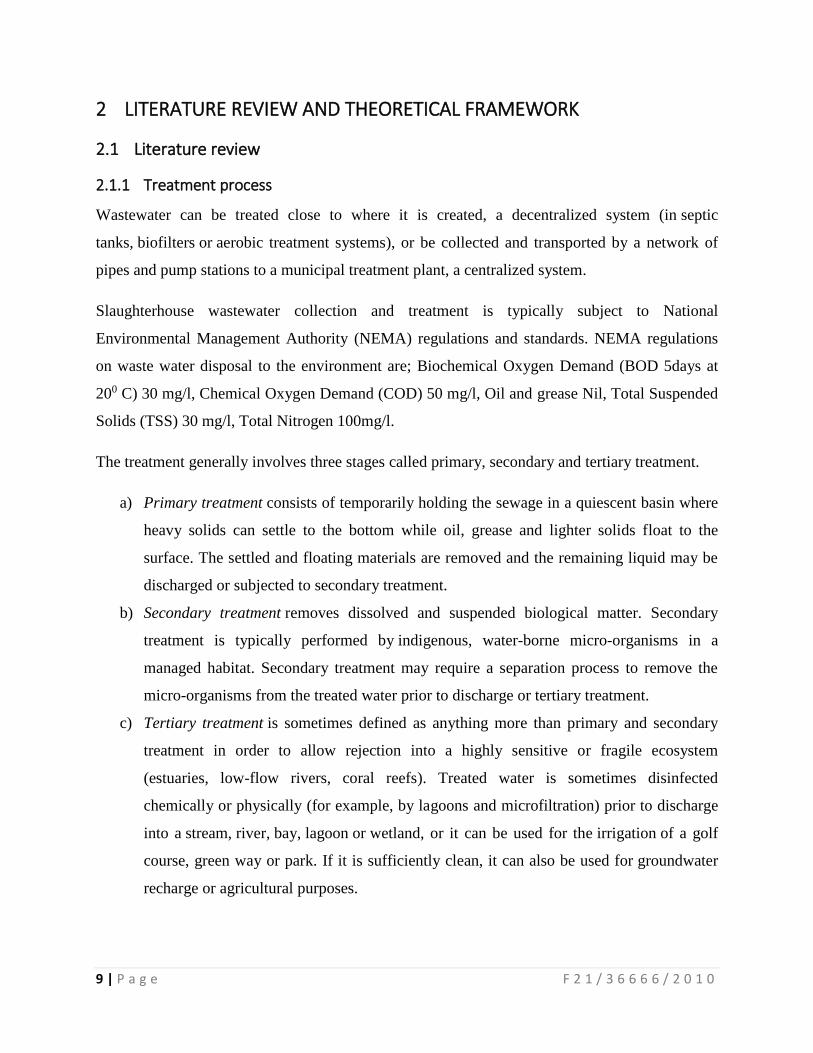
The treatment generally involves three stages called primary, secondary and tertiary treatment.

a) Primary treatment consists of temporarily holding the sewage in a quiescent basin where

heavy solids can settle to the bottom while oil, grease and lighter solids float to the

surface. The settled and floating materials are removed and the remaining liquid may be

discharged or subjected to secondary treatment.

b) Secondary treatment removes dissolved and suspended biological matter. Secondary

treatment is typically performed by indigenous, water-borne micro-organisms in a

managed habitat. Secondary treatment may require a separation process to remove the

micro-organisms from the treated water prior to discharge or tertiary treatment.

c) Tertiary treatment is sometimes defined as anything more than primary and secondary

treatment in order to allow rejection into a highly sensitive or fragile ecosystem

(estuaries, low-flow rivers, coral reefs). Treated water is sometimes disinfected

chemically or physically (for example, by lagoons and microfiltration) prior to discharge

into a stream, river, bay, lagoon or wetland, or it can be used for the irrigation of a golf

course, green way or park. If it is sufficiently clean, it can also be used for groundwater

recharge or agricultural purposes.

10 | P a g e F 2 1 / 3 6 6 6 6 / 2 0 1 0

Figure 2.1 Simplified process flow diagram for a typical large-scale treatment plant.

(Wikipedia Retrieved on 3rd November, 2014).

2.1.2 Anaerobic process for waste water treatment

Anaerobic digestion is a collection of processes by which microorganisms break down

biodegradable material in the absence of oxygen. Anaerobic process uses organic waste to both

produce renewable energy (electricity and heat), and to reduce the bulk of organic waste. By

creating energy and reducing waste, digesters are both an appealing solution to common

problems and an attractive investment. For farmers, food processors and other agriculture

industries, energy from an anaerobic digester reduces or eliminates the need to purchase energy,

surplus energy fed into the electric or gas grid provides income in the form of a feed in tariff, and

the reduction in waste volume protects against rising landfill taxes and gate fees. (NNFCC

Renewable Fuels and energy, 2014)

2.1.2.1 Anaerobic microorganisms and their roles.

Anaerobic microorganisms are organisms whose respiratory energy is generated using electron

acceptors other than oxygen. Some of the electron acceptors used in anaerobic respiration

include; ferric iron (Fe3+), sulphate (SO42-), carbonate (CO3

2-) and certain organic compounds.

11 | P a g e F 2 1 / 3 6 6 6 6 / 2 0 1 0

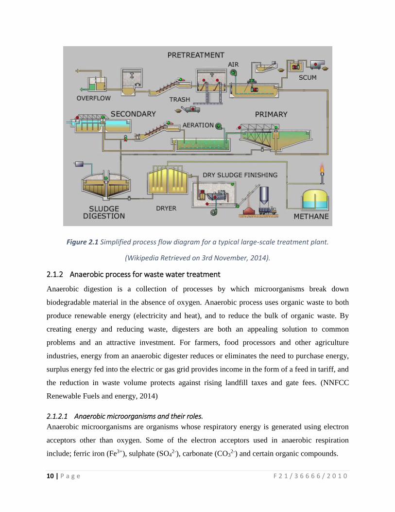
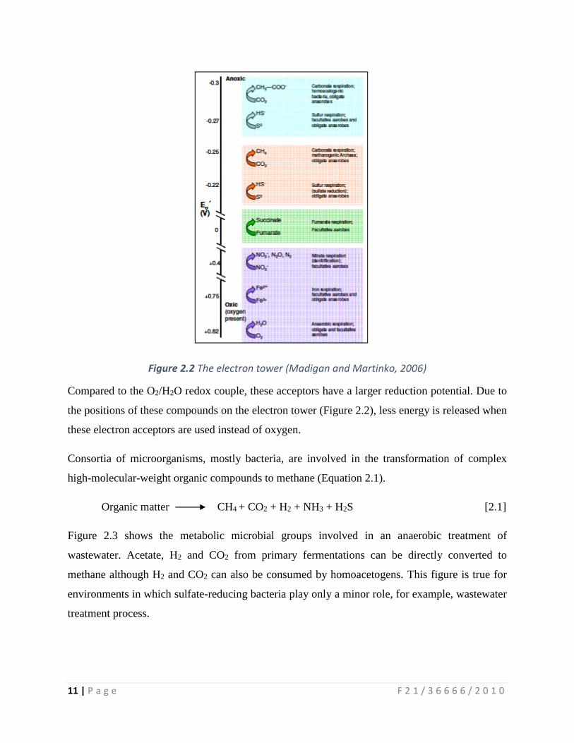
Figure 2.2 The electron tower (Madigan and Martinko, 2006)

Compared to the O2/H2O redox couple, these acceptors have a larger reduction potential. Due to

the positions of these compounds on the electron tower (Figure 2.2), less energy is released when

these electron acceptors are used instead of oxygen.

Consortia of microorganisms, mostly bacteria, are involved in the transformation of complex

high-molecular-weight organic compounds to methane (Equation 2.1).

Organic matter CH4 + CO2 + H2 + NH3 + H2S [2.1]

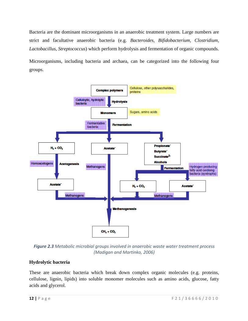
Figure 2.3 shows the metabolic microbial groups involved in an anaerobic treatment of

wastewater. Acetate, H2 and CO2 from primary fermentations can be directly converted to

methane although H2 and CO2 can also be consumed by homoacetogens. This figure is true for

environments in which sulfate-reducing bacteria play only a minor role, for example, wastewater

treatment process.

12 | P a g e F 2 1 / 3 6 6 6 6 / 2 0 1 0

Bacteria are the dominant microorganisms in an anaerobic treatment system. Large numbers are

strict and facultative anaerobic bacteria (e.g. Bacteroides, Bifidobacterium, Clostridium,

Lactobacillus, Streptococcus) which perform hydrolysis and fermentation of organic compounds.

Microorganisms, including bacteria and archaea, can be categorized into the following four

groups.

Figure 2.3 Metabolic microbial groups involved in anaerobic waste water treatment process (Madigan and Martinko, 2006)

Hydrolytic bacteria

These are anaerobic bacteria which break down complex organic molecules (e.g. proteins,

cellulose, lignin, lipids) into soluble monomer molecules such as amino acids, glucose, fatty

acids and glycerol.

13 | P a g e F 2 1 / 3 6 6 6 6 / 2 0 1 0

Eastman and Ferguson (1981) reported that the degradation of particulate organic matter and not

the fermentation of the soluble hydrolysis products is rate limiting as they found no accumulation

of hydrolysis products in their reactor. Hydrolysis reaction is also known to be relatively slow

especially when there are high levels of cellulose and lignin in the wastewater.

Fermentative bacteria

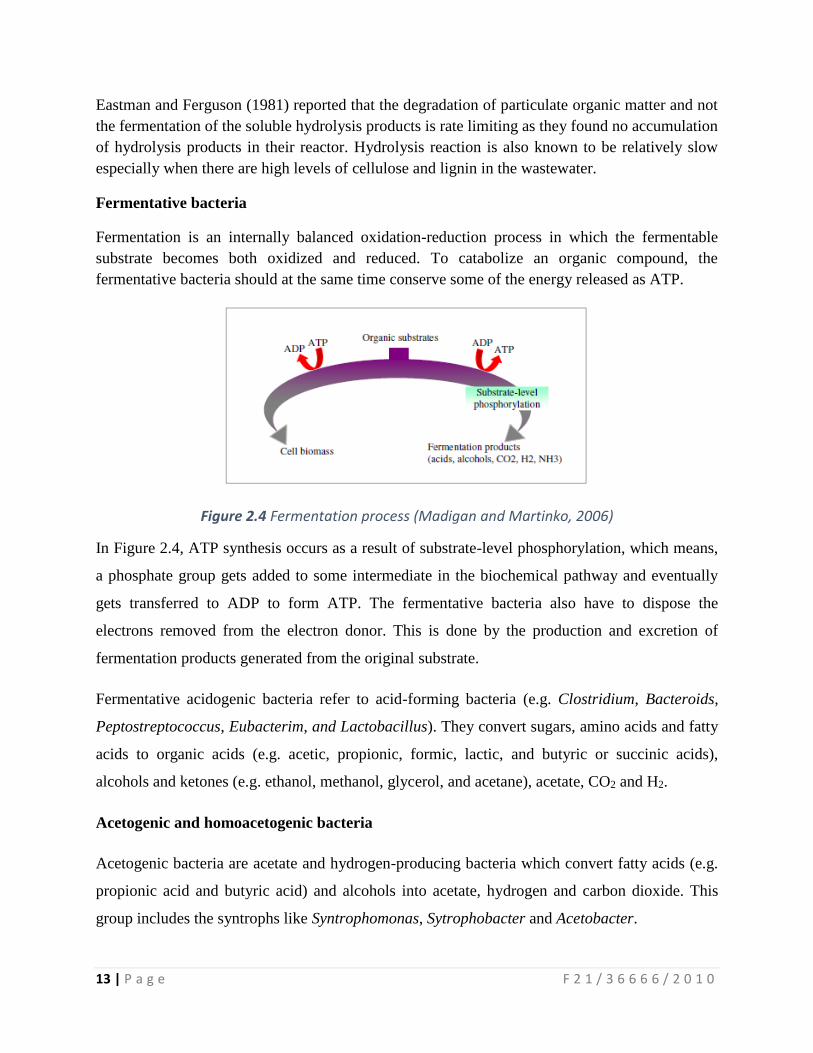
Fermentation is an internally balanced oxidation-reduction process in which the fermentable

substrate becomes both oxidized and reduced. To catabolize an organic compound, the

fermentative bacteria should at the same time conserve some of the energy released as ATP.

Figure 2.4 Fermentation process (Madigan and Martinko, 2006)

In Figure 2.4, ATP synthesis occurs as a result of substrate-level phosphorylation, which means,

a phosphate group gets added to some intermediate in the biochemical pathway and eventually

gets transferred to ADP to form ATP. The fermentative bacteria also have to dispose the

electrons removed from the electron donor. This is done by the production and excretion of

fermentation products generated from the original substrate.

Fermentative acidogenic bacteria refer to acid-forming bacteria (e.g. Clostridium, Bacteroids,

Peptostreptococcus, Eubacterim, and Lactobacillus). They convert sugars, amino acids and fatty

acids to organic acids (e.g. acetic, propionic, formic, lactic, and butyric or succinic acids),

alcohols and ketones (e.g. ethanol, methanol, glycerol, and acetane), acetate, CO2 and H2.

Acetogenic and homoacetogenic bacteria

Acetogenic bacteria are acetate and hydrogen-producing bacteria which convert fatty acids (e.g.

propionic acid and butyric acid) and alcohols into acetate, hydrogen and carbon dioxide. This

group includes the syntrophs like Syntrophomonas, Sytrophobacter and Acetobacter.

14 | P a g e F 2 1 / 3 6 6 6 6 / 2 0 1 0

Ethanol, propionic acid and butyric acid are converted to acetic acid by acetogenic bacteria via

the reactions shown in Equation 2.2 to 2.4.

CH3CH2OH + H2O CH3COOH + 2 H2 [2.2]

CH3CH2COOH + H2O CH3COOH + CO2 + 3 H2 [2.3]

CH3(CH2)2COOH + 2 H2O 2CH3COOH + 2 H2 [2.4]

The production of acetate or certain other fatty acids is energetically advantageous because it

allows the organism to make ATP by substrate-level phosphorylation.

Homoacetogens are a group of strictly anaerobic prokaryotes which can, similar to methanogens,

use CO2 as an electron acceptor in energy metabolism. CO2 is abundant in anaerobic

environment because it is a major product of energy metabolism of chemoorganotrophs.

Hydrogen is the major electron donor for both two types of microorganisms.

Homoacetogens are categorized together because of their pathway of CO2 reduction, i.e. the

acetyl-CoA pathway. Acetyl-CoA pathway is not a cycle, it involves the reduction of CO2 via

two linear pathways, one molecule of CO2 is reduced to the methyl group of acetate and the other

is reduced to the carbonyl group. This is an overall energy-conserving reaction thus,

homoacetogens can grow at the expense of it. However, additional energy-conserving steps

occur because of a sodium motive force established across the cytoplasmic membrane during

acetogenesis. This allows for further energy conservation.

Methanogens

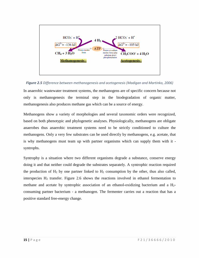
Methanogens are a group of strictly anaerobic Archaea which carry out methanogenesis.

Methanogenesis is a series of complex reactions which involve novel coenzymes. Similar to

acetogenesis, methanogens use CO2 as the electron acceptor and hydrogen as a major electron

donor. However there is a difference in free energy released (Figure 2.5).

15 | P a g e F 2 1 / 3 6 6 6 6 / 2 0 1 0

Figure 2.5 Difference between methanogenesis and acetogenesis (Madigan and Martinko, 2006)

In anaerobic wastewater treatment systems, the methanogens are of specific concern because not

only is methanogenesis the terminal step in the biodegradation of organic matter,

methanogenesis also produces methane gas which can be a source of energy.

Methanogens show a variety of morphologies and several taxonomic orders were recognized,

based on both phenotypic and phylogenetic analyses. Physiologically, methanogens are obligate

anaerobes thus anaerobic treatment systems need to be strictly conditioned to culture the

methanogens. Only a very few substrates can be used directly by methanogens, e.g. acetate, that

is why methanogens must team up with partner organisms which can supply them with it -

syntrophs.

Syntrophy is a situation where two different organisms degrade a substance, conserve energy

doing it and that neither could degrade the substrates separately. A syntrophic reaction required

the production of H2 by one partner linked to H2 consumption by the other, thus also called,

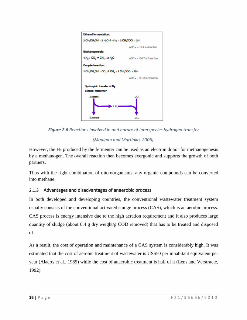
interspecies H2 transfer. Figure 2.6 shows the reactions involved in ethanol fermentation to

methane and acetate by syntrophic association of an ethanol-oxidizing bacterium and a H2-

consuming partner bacterium - a methanogen. The fermenter carries out a reaction that has a

positive standard free-energy change.

16 | P a g e F 2 1 / 3 6 6 6 6 / 2 0 1 0

Figure 2.6 Reactions involved in and nature of interspecies hydrogen transfer

(Madigan and Martinko, 2006).

However, the H2 produced by the fermenter can be used as an electron donor for methanogenesis

by a methanogen. The overall reaction then becomes exergonic and supports the growth of both

partners.

Thus with the right combination of microorganisms, any organic compounds can be converted

into methane.

2.1.3 Advantages and disadvantages of anaerobic process

In both developed and developing countries, the conventional wastewater treatment system

usually consists of the conventional activated sludge process (CAS), which is an aerobic process.

CAS process is energy intensive due to the high aeration requirement and it also produces large

quantity of sludge (about 0.4 g dry weight/g COD removed) that has to be treated and disposed

of.

As a result, the cost of operation and maintenance of a CAS system is considerably high. It was

estimated that the cost of aerobic treatment of wastewater is US$50 per inhabitant equivalent per

year (Alaerts et al., 1989) while the cost of anaerobic treatment is half of it (Lens and Verstraete,

1992).

17 | P a g e F 2 1 / 3 6 6 6 6 / 2 0 1 0

Anaerobic process thus becomes an attractive alternative for tropical or subtropical countries.

The advantages of adopting anaerobic process for treatment include:

a) Biogas (methane, carbon dioxide or hydrogen) can be generated and tapped to recover

energy.

b) Low production of biomass per unit of organics removed.

c) No aeration required.

d) Very high active biomass densities (1% to 3%) can be achieved under favorable

conditions. This means that volumetric reaction times can be increased, reactor size

decreased and the system’s resistance to shock loadings and toxic compounds can be

strengthened.

e) Lower requirement for inorganic nutrients, e.g. nitrogen and phosphorus, due to lower

biomass yields.

f) Anaerobic systems can be left dormant without feeding for extended periods without

severe deterioration in biomass properties. This means that they can be brought back into

service at normal treatment efficiency within very short period of time.

Despite the well-known advantages of anaerobic treatment, there are some disadvantages when

compared to aerobic treatment.

a) Generally lower substrate removal rates per unit of biomass, typically 1/3 to 1/10 those of

aerobic treatment of similar substrate. This is because anaerobic biodegradation of

organics is usually incomplete, often leaving as much as 50% of the organic matter

unconverted (Chynoweth, 1996).

b) Growth of anaerobic organisms is slow. Hence, anaerobic systems can fail if it is unable

to retain its biomass. Low substrate removal rates and low biomass yields result in a

significantly longer time for initial system start-up and recovery after an upset (1 to 6

months).

However, it is also this characteristic that makes anaerobic system advantageous over

aerobic systems. Low biomass yields lead to low sludge production rate which would

reduce the cost of sludge disposal.

c) High operating temperature required for efficient performance. This limits the application

of anaerobic treatment to tropical or sub-tropical regions

18 | P a g e F 2 1 / 3 6 6 6 6 / 2 0 1 0

d) Under short hydraulic retention times, it is difficult to avoid accumulation of excessive

residual organic matter and intermediate products such as volatile fatty acids, especially

conventional continuous-flow suspended growth anaerobic reactors.

e) The chemically reduced conditions necessary for anaerobic process produce H2S,

mercaptans, organic acids and aldehydes, which are corrosive and toxic to

microorganisms in the system. Anaerobically-treated effluents usually still contain a

substantial amount of pathogens, particles, organic and inorganic compounds as well as

ammonia, sulfide and phosphate.

f) Sensitive to certain inhibitory and toxic compounds, such as oxidants (O2, H2O2, Cl2),

H2S, HCN, SO3- and some aromatics.

g) Wilén et al. (2000) reported anaerobic conditions can cause deflocculation of biomass in

the wastewater which only incurred initially in the case of aerobic conditions. This is of a

major concern because the quality of effluent is highly dependent on the efficiency of the

solid-liquid separation process. Eikelboom and van Buijsen (1983) explained that the

growth of anaerobic or facultative anaerobic bacteria between the flocs or the dying of

strictly aerobic organisms in the flocs is the cause of deflocculation.

2.1.4 Common applications of anaerobic process

Anaerobic treatment systems were found in a widespread of applications, especially for

industrial wastewaters like sugar beet, slaughterhouse, starch brewery wastewaters, piggery

wastewaters etc. The loadings ranged from 1 to 50 kg COD/m3, the temperatures from 10 to 650

C and HRT from a few hours to a few days. (Metcalf and Eddy, 2003)

Lettinga et al. (1997) and Verstraete and Vandevivere (1999) reviewed the new generations of

high-rate anaerobic treatment system, such as; Anaerobic contact process (ACP), Anaerobic

baffled reactor (ABR), Upflow Anaerobic Sludge Blanket (UASB), Expanded Granular Sludge

Bed (EGSB) and Staged Multi-Phase Anaerobic (MPSA) reactor systems, Anaerobic Sequencing

Batch Reactor (ASBR). These systems have a higher efficiency at higher loading rates. In

addition, they are applicable for extreme environmental conditions (e.g. low and high

temperatures) and to inhibitory compounds.

They can even perform anaerobic ammonium oxidation (anammox) and chemical phosphorus

precipitation. By integrating these processes with other biological methods (sulphate reduction,

19 | P a g e F 2 1 / 3 6 6 6 6 / 2 0 1 0

micro-aerophilic organisms) and with physical-chemical methods, the cost of treatment of

wastewater can be reduced while at the same time valuable components can be recovered for

reuse.

2.1.5 Applicability of anaerobic process for slaughterhouse wastewater

To study the applicability of anaerobic process for slaughterhouse wastewater, first, the

characteristics of slaughterhouse wastewater has to be understood. The important parameters

which has to be noted include BOD, COD, suspended solids, oil, grease and concentration of

chlorinated compounds (Lawrence, 2006), presence of surfactants and size of particles (Tarek,

2001).

In Kenya, various slaughterhouse wastewater systems have been adopted. These include;

anaerobic lagoons, anaerobic contact reactor (ACR), anaerobic sequencing batch reactor (ASBR)

and Upflow anaerobic sludge blanket (UASB). Dagoretti’s Nyongara Slaughterhouse uses

anaerobic (fixed dome) reactor to produce biogas. Some of the slaughterhouses integrate two of

the above systems as their wastewater management system. However there’s needed to devise a

best preferred anaerobic process that requires a low capital equipment investment and results in

efficient operation.

Table 2.1 Typical operating conditions of various AD configurations

Reactor type Load (kg COD/m3 day) HRT (hour) COD removal (%)

Conventional anaerobic reactor 1 – 5 240 - 360 60 – 80

Anaerobic contact reactor 1 – 6 24 - 120 70 – 95

Anaerobic sequence batch reactor 1 – 10 6 - 24 75 – 90

Anaerobic filter 2 – 15 10 - 85 80 – 95

Fluidized bed 2 – 50 1 - 4 80 – 90

UASB 2 – 30 2 - 72 80 – 95

Anaerobic baffled reactor 3 – 35 9 - 32 75 – 95

Source: Anaerobic reactor technologies, 2014

20 | P a g e F 2 1 / 3 6 6 6 6 / 2 0 1 0

Based on COD load per day, table 2.1 shows that anaerobic sequence batch reactor is the most

appropriate technology due to its high efficiency for both COD removal at a minimum HRT as

compared to the other anaerobic reactor technologies.

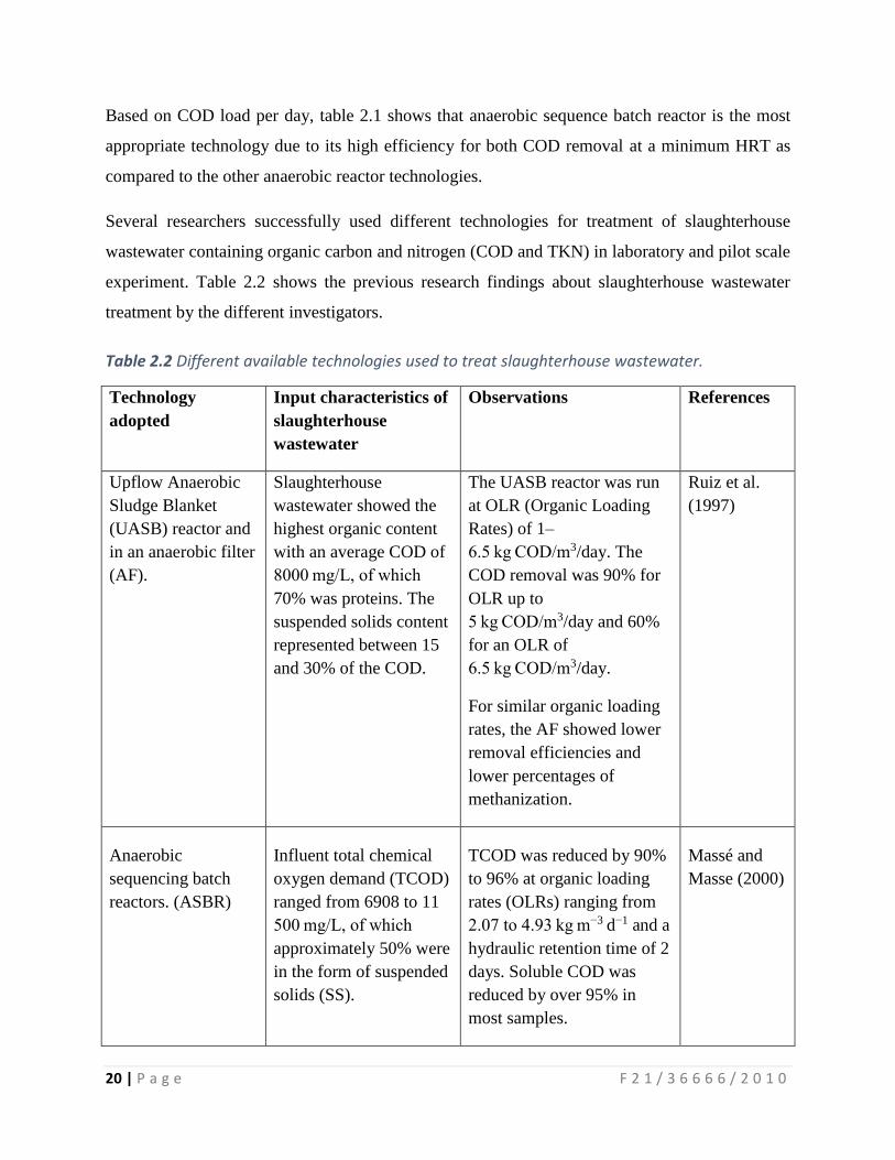
Several researchers successfully used different technologies for treatment of slaughterhouse

wastewater containing organic carbon and nitrogen (COD and TKN) in laboratory and pilot scale

experiment. Table 2.2 shows the previous research findings about slaughterhouse wastewater

treatment by the different investigators.

Table 2.2 Different available technologies used to treat slaughterhouse wastewater.

Technology

adopted

Input characteristics of

slaughterhouse

wastewater

Observations References

Upflow Anaerobic

Sludge Blanket

(UASB) reactor and

in an anaerobic filter

(AF).

Slaughterhouse

wastewater showed the

highest organic content

with an average COD of

8000 mg/L, of which

70% was proteins. The

suspended solids content

represented between 15

and 30% of the COD.

The UASB reactor was run

at OLR (Organic Loading

Rates) of 1–

6.5 kg COD/m3/day. The

COD removal was 90% for

OLR up to

5 kg COD/m3/day and 60%

for an OLR of

6.5 kg COD/m3/day.

For similar organic loading

rates, the AF showed lower

removal efficiencies and

lower percentages of

methanization.

Ruiz et al.

(1997)

Anaerobic

sequencing batch

reactors. (ASBR)

Influent total chemical

oxygen demand (TCOD)

ranged from 6908 to 11

500 mg/L, of which

approximately 50% were

in the form of suspended

solids (SS).

TCOD was reduced by 90%

to 96% at organic loading

rates (OLRs) ranging from

2.07 to 4.93 kg m−3 d−1 and a

hydraulic retention time of 2

days. Soluble COD was

reduced by over 95% in

most samples.

Massé and

Masse (2000)

21 | P a g e F 2 1 / 3 6 6 6 6 / 2 0 1 0

Fixed bed

sequencing batch

reactor (FBSBR).

The wastewater has

COD loadings in the

range of 0.5–

1.5 Kg COD/m3 per day.

COD, TN, and phosphorus

removal efficiencies were at

range of 90–96%, 60–88%,

and 76–90%, respectively

Rahimi et al.

(2011)

Hybrid upflow

anaerobic sludge

blanket (HUASB)

reactor for treating

poultry

slaughterhouse

wastewater.

Slaughterhouse

wastewater showed total

COD 3000–4800 mg/L,

soluble COD 1030–

3000 mg/L, BOD5 750–

1890 mg/L, suspended

solids 300–950 mg/L,

alkalinity (as CaCO3)

600–1340 mg/L, VFA

(as acetate) 250–

540 mg/L, and pH 7–7.6.

The HUSB reactor was run

at OLD of

19 kg COD/m3/day and

achieved TCOD and SCOD

removal efficiencies of 70–

86% and 80–92%,

respectively.

The biogas was varied

between 1.1 and 5.2 m3/m3 d

with the maximum methane

content of 72%.

Rajakumar et

al. (2012)

Anaerobic hybrid

reactor was packed

with light weight

floating media.

COD, BOD and

Suspended Solids in the

range of 22000–

27500 mg/L, 10800–

14600 mg/L, and 1280–

1500 mg/L, respectively

COD and BOD reduction

was found in the range of

86.0–93.58% and 88.9–

95.71%, respectively.

Sunder &

Satyanarayan

(2013)

Sequencing batch reactors (SBRs) are advocated as one of the best available techniques (BATs)

for slaughterhouse wastewater treatment (European Commission, 2005 and Mahvi 2008) because

they are capable of removing organic carbon, nutrients, and suspended solids from wastewater in

a single tank and also have low capital and operational costs.

A full-scale SBR system was evaluated by Lo and Liao (2007) to remove 82% of BOD and more

than 75% of nitrogen after a cycle period of 4.6 hour from swine wastewater. Mahvi et al. (2004)

carried out a pilot-scale study on removal of nitrogen both from synthetic and domestic

wastewater in a continuous flow SBR and obtained a total nitrogen and TKN removal of 70–80%

and 85–95%, respectively. An SBR system demonstrated by Lemaire et al. (2009) to high degree

of biological remove of nitrogen, phosphorus, and COD to very low levels from slaughterhouse

wastewater. A high degree removal of total phosphorus (98%), total nitrogen (97%), and total

COD (95%) was achieved after a 6-hour cycle period.

22 | P a g e F 2 1 / 3 6 6 6 6 / 2 0 1 0

2.1.6 Anaerobic Sequencing Batch Reactor (ASBR)

2.1.6.1 Concepts of a sequence batch reactor

Sequencing batch reactors (SBR) are industrial processing tanks for the treatment of wastewater.

SBR reactors treat wastewater such as sewage or mechanical biological treatment facilities in

batches. Oxygen is bubbled through the wastewater to reduce biochemical oxygen

demand (BOD) and chemical oxygen demand (COD) which makes the effluent suitable for

discharge to surface waters or for use on land. (Wikipedia, 2014)

A batch reactor is characterized such that there is neither continuous flow of wastewater entering

nor leaving the reactor (i.e. flow enters, is treated, discharged and the cycle repeats). The content

is completely mixed (Metcalf and Eddy, 2003).

While there are several configurations of SBRs, the basic process is similar. The installation

consists of at least two identically equipped tanks with a common inlet, which can be switched

between them. The tanks have a “flow through” system, with raw wastewater (influent) coming

in at one end and treated water (effluent) flowing out the other. While one tank is in settle/decant

mode the other is aerating and filling. At the inlet is a section of the tank known as the bio-

selector. This consists of a series of walls or baffles which direct the flow either from side to side

of the tank or under and over consecutive baffles. This helps to mix the incoming Influent and

the returned activated sludge (RAS), beginning the biological digestion process before the liquor

enters the main part of the tank.

2.1.6.2 Treatment stages

A sequencing batch reactor (SBR) provides for time sequencing of operations which include

equalization, biological conversion, sedimentation and clarification all in one complete cycle.

The SBR process has four main phases, i.e. fill, react, settle and decant. A fifth optional phase is

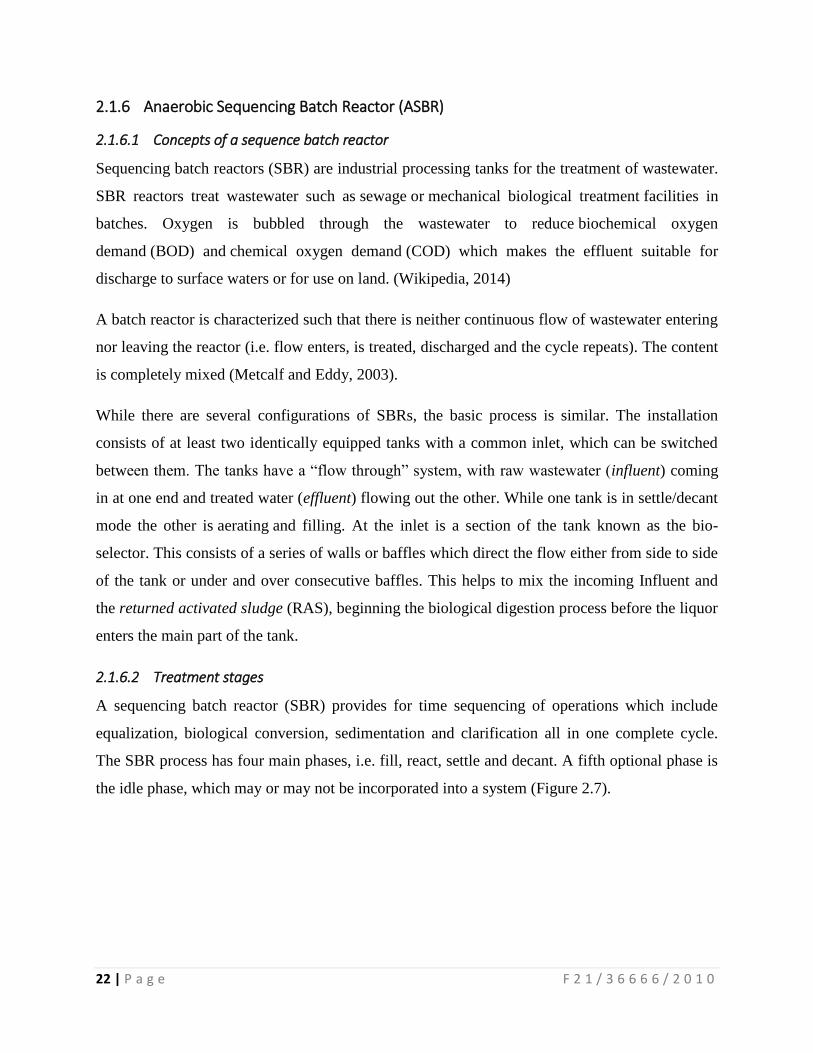
the idle phase, which may or may not be incorporated into a system (Figure 2.7).

23 | P a g e F 2 1 / 3 6 6 6 6 / 2 0 1 0

Figure 2.7 Different phases of a batch reactor in one operating cycle. (Wong, 2007) Fill

The wastewater that is to be treated can be fed into the system through several methods.

Organic contact and biological reactions are minimized by feeding in the wastewater at

any rate in a quiescent manner near the liquid surface until the tank is full.

Wastewater is fed at a low rate with mixing to allow reaction to begin as soon as Fill

phase starts. Thus, substrate concentration is still held relatively low.

Wastewater is fed at a rate equal to the effluent discharge rate which means the system

acts as an equalization tank.

Wastewater is added as a batch dump inflow or any other desired inflow rate and

accompanying mixing method to meet the specific treatment objectives.

After the Fill phase, any variations in the wastewater influent no longer have any effect on the

treatment processes taking place inside the reactor except to limit or extend the total time

allowed for them to take place.

Typically, an anaerobic sequencing batch reactor is operated with a fast fill, leading to a low fill

time to cycle time ratio. This operating strategy provides a high initial substrate concentration.

24 | P a g e F 2 1 / 3 6 6 6 6 / 2 0 1 0

This will enable zero order kinetics with respect to the organic acids that form, which may lead

to an acid formation problem. However, this phenomenon is more severe if a high strength

wastewater is being treated.

React

React phase follows the Fill phase. This is the main period when biodegradation takes place.

Mixing is provided to ensure sufficient contact of the microorganisms with the substrate.

Organics in the wastewater can be acclimatized by exposing them to high substrate levels for a

short period of time and low levels for a longer period of time.

Similarly, it can be done by maintaining a relatively low substrate level during most of the Fill

and React phase. High substrate concentration in the reactor in the beginning of the react phase

allows a high food-to-microorganisms (F/M) ratio, which means the rate of substrate uptake is

high.

Settle

In the settle phase, solid-liquid separation is allowed to take place by gravitational force. Biogas

attached to or entrapped by biological solids can also be separated and collected.

After the React phase, substrate concentration in the reactor is low, meaning that the F/M ratio is

low. A low F/M is known to improve the settling properties of biomass. High settling velocities

of the biomass in the SBR is expected. Heavy flocs of diameter more than 1 mm can sweep

down aggregates of smaller flocs. These heavy flocs are able to form due to the operation regime

of the SBR. The gentle stirring of the mixed liquor supports flocculation and during the Settle

phase, quiescent conditions are provided to aid in settling.

Decant

The treated effluent is withdrawn from the system from above the sludge blanket. It is usually

done at a slow rate to minimize disturbance of the settled solids.

A SBR is also different from other fill and draw systems. It is filled and drawn within a defined

period of time so variations in the influent of the treatment plant has no effect on the process

after the fill phase of the particular cycle has ended. The cycle is continuously repeated in a

defined and regulated variation of process conditions.

25 | P a g e F 2 1 / 3 6 6 6 6 / 2 0 1 0

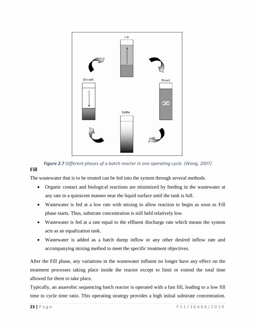
Figure 2.8 A schematic diagram of the experimental setup

26 | P a g e F 2 1 / 3 6 6 6 6 / 2 0 1 0

2.2 Theoretical Framework

2.2.1 Biochemical Oxygen Demand (BOD)

The Biochemical Oxygen Demand (BOD) is the amount of dissolved oxygen which is used up

by these microorganisms and is roughly equivalent to the amount of organic matter found in the

wastewater. The more organic matter that is present in the water, the more dissolved oxygen will

be used up by the bacteria and the greater the BOD reading will be.

Wastewater treatment plants use BOD as an estimate of the waste load in the influent water.

They can also test BOD of the effluent to determine the plant's efficiency, to control plant

processes, and to determine the effects of discharges on receiving waters.

BOD5 is determined through determination of initial and final dissolve oxygen of the wastewater

in the laboratory. From these parameters, BOD5 is calculated as illustrated in equations 2.4 and

2.6.

When dilution water is not seeded:

BOD5, mg/L = 𝐷1− 𝐷2

𝑃 [2.5]

When dilution water is seeded:

BOD5, mg/L = (𝐷1− 𝐷2)−(𝐵1− 𝐵2)

𝑃 [2.6]

Where:

D1 = Dissolved oxygen of diluted sample immediately after preparation, mg/L,

D2 = Dissolved oxygen of diluted sample after 5 d incubation at 200C, mg/L,

P = Decimal volumetric fraction of sample used,

B1 = Dissolved oxygen of seed control before incubation, mg/L,

B2 = Dissolved oxygen of seed control after incubation mg/L

27 | P a g e F 2 1 / 3 6 6 6 6 / 2 0 1 0

f = ratio of seed in diluted sample to seed in seed control

f = % 𝑠𝑒𝑒𝑑 𝑖𝑛 𝑑𝑖𝑙𝑢𝑡𝑒𝑑 𝑠𝑎𝑚𝑝𝑙𝑒

% 𝑠𝑒𝑒𝑑 𝑖𝑛 𝑠𝑒𝑒𝑑 𝑐𝑜𝑛𝑡𝑟𝑜𝑙 [2.7]

If seed material is added directly to sample or to seed control bottles

f = 𝑣𝑜𝑙𝑢𝑚𝑒 𝑜𝑓 𝑠𝑒𝑒𝑑 𝑖𝑛 𝑑𝑖𝑙𝑢𝑡𝑒𝑑 𝑠𝑎𝑚𝑝𝑙𝑒

𝑣𝑜𝑙𝑢𝑚𝑒 𝑜𝑓 𝑠𝑒𝑒𝑑 𝑖𝑛 𝑠𝑒𝑒𝑑 𝑐𝑜𝑛𝑡𝑟𝑜𝑙 [2.8]

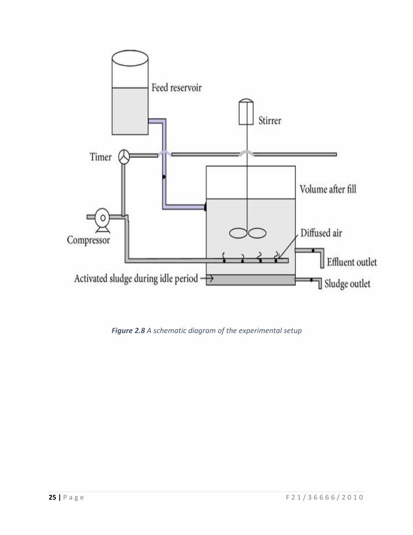
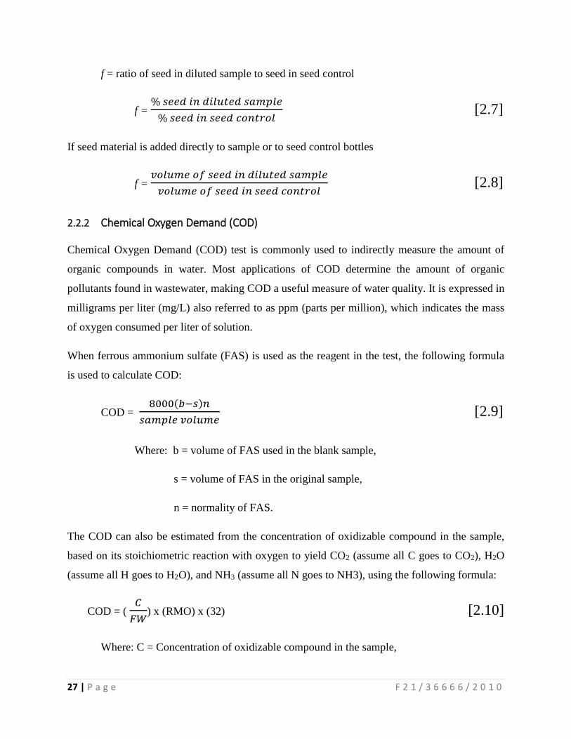
2.2.2 Chemical Oxygen Demand (COD)

Chemical Oxygen Demand (COD) test is commonly used to indirectly measure the amount of

organic compounds in water. Most applications of COD determine the amount of organic

pollutants found in wastewater, making COD a useful measure of water quality. It is expressed in

milligrams per liter (mg/L) also referred to as ppm (parts per million), which indicates the mass

of oxygen consumed per liter of solution.

When ferrous ammonium sulfate (FAS) is used as the reagent in the test, the following formula

is used to calculate COD:

COD = 8000(𝑏−𝑠)𝑛

𝑠𝑎𝑚𝑝𝑙𝑒 𝑣𝑜𝑙𝑢𝑚𝑒 [2.9]

Where: b = volume of FAS used in the blank sample,

s = volume of FAS in the original sample,

n = normality of FAS.

The COD can also be estimated from the concentration of oxidizable compound in the sample,

based on its stoichiometric reaction with oxygen to yield CO2 (assume all C goes to CO2), H2O

(assume all H goes to H2O), and NH3 (assume all N goes to NH3), using the following formula:

COD = ( 𝐶

𝐹𝑊) x (RMO) x (32) [2.10]

Where: C = Concentration of oxidizable compound in the sample,

28 | P a g e F 2 1 / 3 6 6 6 6 / 2 0 1 0

FW = Formula weight of the oxidizable compound in the sample,

RMO = Ratio of the number of moles of oxygen to number of moles of oxidizable

compound in their reaction to CO2, water, and ammonia

2.2.3 Total Suspended Solids (TSS)

Concentration of Total Suspended Solids (TSS) in the sample can be calculated using the

following formula:

TSS, mg/L = (𝐴 −𝐵) 𝑥 1000

𝑠𝑎𝑚𝑝𝑙𝑒 𝑣𝑜𝑙𝑢𝑚𝑒,𝑚𝐿 [2.11]

Where: A = Sample and filter weight, mg.

B = Filter weight, mg

If two samples were used, then the average total suspended solids can be calculated as follows:

Average total suspended solids, mg/L = (𝐶 + 𝐷)

2 [2.12]

Where: C = Total suspended solids of sample 1, mg/L

D = Total suspended solids of sample 2, mg/L

2.2.4 Flow rate (Q)/ daily wastewater generation

The flow for the wastewater treatment plants are based on the effluent production from the

slaughterhouse. The flow estimates for a location should show peak, minimum and average flow

rates.

Q = (NC x VC) + (Ng x Vg) [2.13]

Where: NC = number of cattle slaughtered daily.

VC = volume of water used in slaughtering each cattle, litres

Ng = number of goats and sheep slaughtered daily.

SVg = volume of water used in slaughtering each goat/sheep, litres

2.2.5 Volume of the reactor

2.2.5.1 Reactor Working Volume

Active digester volume (V) is the volume occupied by the slurry in the digester and is given as;

V (m3) = Q x HRT (days) [2.14]

Where: Q = Influent flow rate, m3/day

HRT = Hydraulic Retention Time.

29 | P a g e F 2 1 / 3 6 6 6 6 / 2 0 1 0

Influent flow rate depends on the dilution of the waste and therefore the waste should be less

diluted to ensure that a smaller digester is used. Total volume of gas storage is equal to the

volume of gas generated in 24 hours under normal operating conditions. (Nijaguna, 2002)

2.2.5.2 Gas Storage Volume (Vg)

The methane produced in an anaerobic process is proportional to the amount of substrate

removed. The rate of methane production is given by the following equation.

Qm = QM (So – Se) = Q x E x M x So [2.15]

Where: Qm = Gas production rate. .

So = Total influent COD

Se = Total effluent COD

M = volume of CH4 produced per unit of COD removed

Q = Influent Flow Rate

E = Efficiency factor

2.2.6 Solid Retention Time (SRT or Θx)

The Solids Retention Time (SRT) can be described by the mass of sludge in the reactor divided

by the mass removal rate of sludge from the reactor.

SRT or Θx = 𝑉𝑋𝑣

𝑄𝑤𝑋𝑤 [2.16]

Where: Qw = Volumetric flow rate of waste solids from system

Xw = VSS concentration in Qw

V = Volume of reactor

Xv = Average concentration of VSS in reactor

2.2.7 Hydraulic Retention Time (HRT),

Also known as Hydraulic Residence Time or t (tau), is a measure of the average length

of time that a soluble compound remains in a constructed bioreactor.

HRT (hours/days) = 𝑉

𝑄 [2.17]

Where: V = Volume of the reactor in m3 or litres

Q = Influent flow rate, m3/h or litres/day

30 | P a g e F 2 1 / 3 6 6 6 6 / 2 0 1 0

3 GENERATION OF CONCEPT DESIGN

3.1 Description of the design project methodology

Literature reviews and consultation with waste experts was conducted so as to develop

background knowledge about the wastewater treatment and learn how to address design

challenges that affect efficiencies of the existing wastewater treatment systems.

Observations were made to determine the wastewater disposal and management at the Bahati

slaughterhouse. Information was also obtained from staff about their work responsibilities and

operations at the slaughterhouse.

Past review of literature on the past studies in this study area were carried out in order to form a

basis of the design. This helped in identifying the need and develop the insights, thus

determining the modifications viable to improve the efficiency of slaughterhouse wastewater

treatment.

Analysis of engineering principles governing wastewater treatment and structural design of a

WWTP were carried out in order to identify parameters that will require consideration in the

entire course of the project. Relevant standards and conditions of wastewater disposal as

stipulated by NEMA were considered.

3.2 Data Collection

The data was collected from; Slaughterhouse officials, local residents, NEMA officials, Nairobi

City Water and Sewerage Company, weather stations, and Kenya Agricultural Research Institute

(KARI).

3.3 Location of the project

Geotechnical survey was carried out to determine the optimum location of the treatment plant in

the proposed site and whether the available space/land is sufficient for the proposed wastewater

management system.

31 | P a g e F 2 1 / 3 6 6 6 6 / 2 0 1 0

3.4 Data collected and its uses to address objectives

The information on the quantity of daily wastewater production was obtained through flow

measurement and interviewing the slaughterhouse officials on the estimates of the amount of

water they use every day.

Wastewater Samples were collected and its content determined through lab tests, (i.e. BOD,

COD, TSS, Oil and Grease content). This was used to analyze the quantity and composition of

slaughterhouse wastewater that could be used in sizing the treatment plant.

Soil samples were collected and tests carried out, these experiments helped in determining the

strength parameters of the soil (cohesion c and angle of angle of internal friction Ф) hence used

to evaluate the shear strength of soil.

3.5 Analysis of the data obtained.

COD, BOD5, TSS, oil-grease content and pH determinations were done according to the standard

methods stipulated by NEMA (Standard for discharge into natural water courses, 2014).

Amount of waste produced, load on the system, sizes of the structures required and population

design period were used to determine the volume of the anaerobic sequence batch rector.

Inlet and outlet flow rates, were also analyzed to determine the design specifications that can be

used in coming up with detailed engineering drawings of the proposed project.

3.6 Modelling the system/making design drawings

After determination of the relevant design specifications, the information was used to come up

with detailed engineering drawings of the proposed project.

32 | P a g e F 2 1 / 3 6 6 6 6 / 2 0 1 0

4 RESULTS AND DATA ANALYSIS

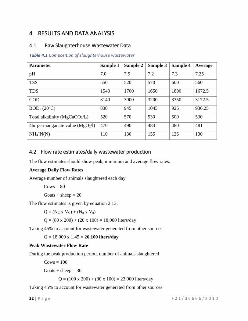
4.1 Raw Slaughterhouse Wastewater Data

Table 4.1 Composition of slaughterhouse wastewater

Parameter Sample 1 Sample 2 Sample 3 Sample 4 Average

pH 7.0 7.5 7.2 7.3 7.25

TSS 550 520 570 600 560

TDS 1540 1700 1650 1800 1672.5

COD 3140 3000 3200 3350 3172.5

BOD5 (200C) 830 945 1045 925 936.25

Total alkalinity (MgCaCO3/L) 520 570 530 500 530

4hr permanganate value (MgO2/l) 470 490 484 480 481

NH4+N(N) 110 130 155 125 130

4.2 Flow rate estimates/daily wastewater production

The flow estimates should show peak, minimum and average flow rates.

Average Daily Flow Rates

Average number of animals slaughtered each day;

Cows = 80

Goats + sheep = 20

The flow estimates is given by equation 2.13;

Q = (NC x VC) + (Ng x Vg)

Q = (80 x 200) + (20 x 100) = 18,000 liters/day

Taking 45% to account for wastewater generated from other sources

Q = 18,000 x 1.45 = 26,100 liters/day

Peak Wastewater Flow Rate

During the peak production period, number of animals slaughtered

Cows = 100

Goats + sheep = 30

Q = (100 x 200) + (30 x 100) = 23,000 liters/day

Taking 45% to account for wastewater generated from other sources

33 | P a g e F 2 1 / 3 6 6 6 6 / 2 0 1 0

Q = 23,000 x 1.45 = 33,350 liters/day

Minimum Flow Rates

During the low production period, number of animals slaughtered

Cows = 60

Goats + sheep = 10

Q = (60 x 200) + (10 x 100) = 13,000 liters/day

Taking 45% to account for wastewater generated from other sources

Q = 13,000 x 1.45 = 18,850 liters/day

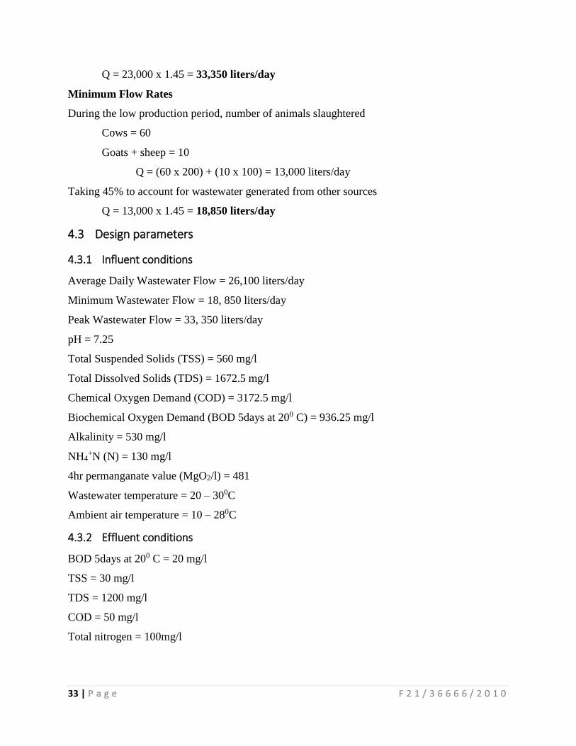
4.3 Design parameters

4.3.1 Influent conditions

Average Daily Wastewater Flow = 26,100 liters/day

Minimum Wastewater Flow = 18, 850 liters/day

Peak Wastewater Flow = 33, 350 liters/day

pH = 7.25

Total Suspended Solids (TSS) = 560 mg/l

Total Dissolved Solids (TDS) = 1672.5 mg/l

Chemical Oxygen Demand (COD) = 3172.5 mg/l

Biochemical Oxygen Demand (BOD 5days at 200 C) = 936.25 mg/l

Alkalinity = 530 mg/l

NH4+N (N) = 130 mg/l

4hr permanganate value (MgO2/l) = 481

Wastewater temperature = 20 – 300C

Ambient air temperature = 10 – 280C

4.3.2 Effluent conditions

BOD 5days at 200 C = 20 mg/l

TSS = 30 mg/l

TDS = 1200 mg/l

COD = 50 mg/l

Total nitrogen = 100mg/l

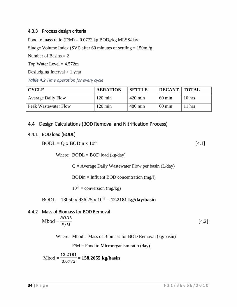
34 | P a g e F 2 1 / 3 6 6 6 6 / 2 0 1 0

4.3.3 Process design criteria

Food to mass ratio (F/M) = 0.0772 kg BOD5/kg MLSS/day

Sludge Volume Index (SVI) after 60 minutes of settling = 150ml/g

Number of Basins = 2

Top Water Level = 4.572m

Desludging Interval > 1 year

Table 4.2 Time operation for every cycle

CYCLE AERATION SETTLE DECANT TOTAL

Average Daily Flow 120 min 420 min 60 min 10 hrs

Peak Wastewater Flow 120 min 480 min 60 min 11 hrs

4.4 Design Calculations (BOD Removal and Nitrification Process)

4.4.1 BOD load (BODL)

BODL = Q x BODin x 10-6 [4.1]

Where: BODL = BOD load (kg/day)

Q = Average Daily Wastewater Flow per basin (L/day)

BODin = Influent BOD concentration (mg/l)

10-6 = conversion (mg/kg)

BODL = 13050 x 936.25 x 10-6 = 12.2181 kg/day/basin

4.4.2 Mass of Biomass for BOD Removal

Mbod = 𝐵𝑂𝐷𝐿

𝐹/𝑀 [4.2]

Where: Mbod = Mass of Biomass for BOD Removal (kg/basin)

F/M = Food to Microorganism ratio (day)

Mbod = 12.2181

0.0772 = 158.2655 kg/basin

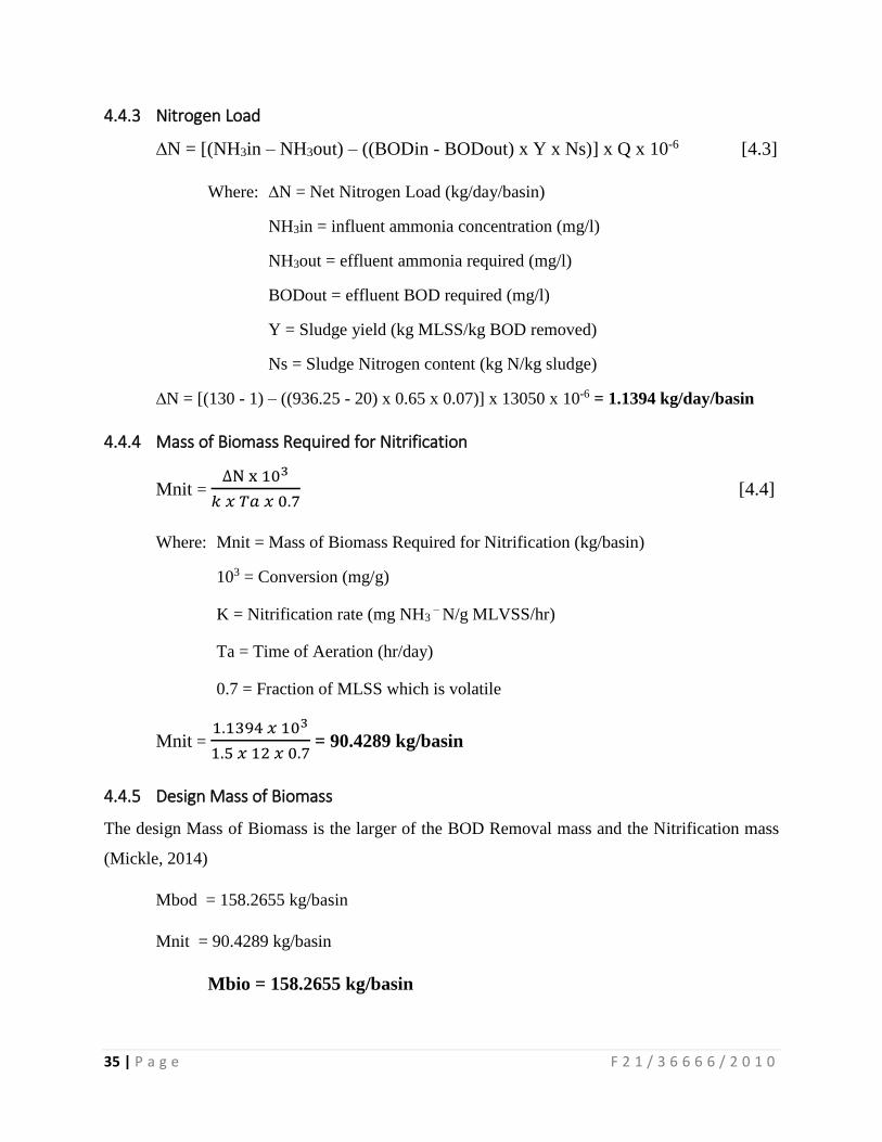
35 | P a g e F 2 1 / 3 6 6 6 6 / 2 0 1 0

4.4.3 Nitrogen Load

∆N = [(NH3in – NH3out) – ((BODin - BODout) x Y x Ns)] x Q x 10-6 [4.3]

Where: ∆N = Net Nitrogen Load (kg/day/basin)

NH3in = influent ammonia concentration (mg/l)

NH3out = effluent ammonia required (mg/l)

BODout = effluent BOD required (mg/l)

Y = Sludge yield (kg MLSS/kg BOD removed)

Ns = Sludge Nitrogen content (kg N/kg sludge)

∆N = [(130 - 1) – ((936.25 - 20) x 0.65 x 0.07)] x 13050 x 10-6 = 1.1394 kg/day/basin

4.4.4 Mass of Biomass Required for Nitrification

Mnit = ∆N x 103

𝑘 𝑥 𝑇𝑎 𝑥 0.7 [4.4]

Where: Mnit = Mass of Biomass Required for Nitrification (kg/basin)

103 = Conversion (mg/g)

K = Nitrification rate (mg NH3 – N/g MLVSS/hr)

Ta = Time of Aeration (hr/day)

0.7 = Fraction of MLSS which is volatile

Mnit = 1.1394 𝑥 103

1.5 𝑥 12 𝑥 0.7 = 90.4289 kg/basin

4.4.5 Design Mass of Biomass

The design Mass of Biomass is the larger of the BOD Removal mass and the Nitrification mass

(Mickle, 2014)

Mbod = 158.2655 kg/basin

Mnit = 90.4289 kg/basin

Mbio = 158.2655 kg/basin

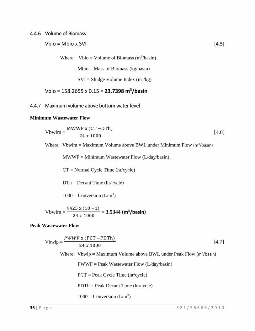
36 | P a g e F 2 1 / 3 6 6 6 6 / 2 0 1 0

4.4.6 Volume of Biomass

Vbio = Mbio x SVI [4.5]

Where: Vbio = Volume of Biomass (m3/basin)

Mbio = Mass of Biomass (kg/basin)

SVI = Sludge Volume Index (m3/kg)

Vbio = 158.2655 x 0.15 = 23.7398 m3/basin

4.4.7 Maximum volume above bottom water level

Minimum Wastewater Flow

Vbwlm = MWWF x (CT −DTh)

24 𝑥 1000 [4.6]

Where: Vbwlm = Maximum Volume above BWL under Minimum Flow (m3/basin)

MWWF = Minimum Wastewater Flow (L/day/basin)

CT = Normal Cycle Time (hr/cycle)

DTh = Decant Time (hr/cycle)

1000 = Conversion (L/m3)

Vbwlm = 9425 x (10 −1)

24 𝑥 1000 = 3.5344 (m3/basin)

Peak Wastewater Flow

Vbwlp = 𝑃𝑊𝑊𝐹 x (PCT −PDTh)

24 𝑥 1000 [4.7]

Where: Vbwlp = Maximum Volume above BWL under Peak Flow (m3/basin)

PWWF = Peak Wastewater Flow (L/day/basin)

PCT = Peak Cycle Time (hr/cycle)

PDTh = Peak Decant Time (hr/cycle)

1000 = Conversion (L/m3)

37 | P a g e F 2 1 / 3 6 6 6 6 / 2 0 1 0

Vbwlp = 16675 x (11 −1)

24 𝑥 1000 = 6.9479 (m3/basin)

MVAB = 6.9479 (m3/basin)

4.4.8 Decant Rates

Minimum Wastewater Flow

MFDR = 𝑀𝑉𝐴𝐵 𝑥 1000

𝐷𝑇 +

𝑀𝑊𝑊𝐹

1440 [4.8]

Where: MFDR = Minimum wastewater Flow Decant Rate (L/min)

DT = normal Decant Time (hr/cycle)

1440 = Conversion (min/day)

MFDR = 6.9479 𝑥 1000

60 +

9425

1440 = 122.34 (L/min)

Peak Wastewater Flow

PWDR = 𝑀𝑉𝐴𝐵 𝑥 1000

𝑃𝐷𝑇 +

𝑃𝑊𝑊𝐹

1440 [4.9]

Where: PWDR = Peak Wastewater Decant Rate (L/min)

PDT = Peak Decant Time (hr/cycle)

PWDR = 6.9479 𝑥 1000

60 +

16675

1440 = 127.38 (L/min)

4.4.9 Decanter Sizing

Minimum Wastewater Flow

DLM = MFDR

0.5 𝑥 1000 [4.10]

Where: DLM = Decanter Length for Minimum Wastewater Flow (m)

0.50 = Design Weir Loading Rate (m3/min/m of decanter weir)

Dld = 122.34

0.50 𝑥 1000 = 0.2447 m

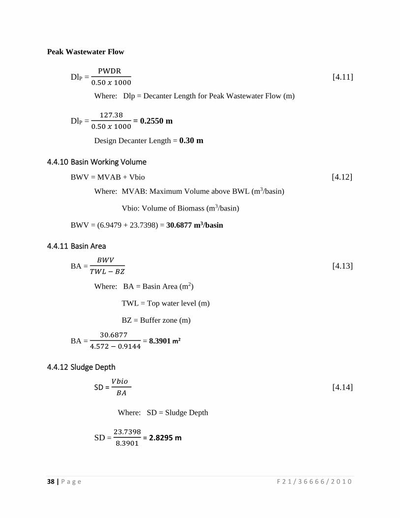
38 | P a g e F 2 1 / 3 6 6 6 6 / 2 0 1 0

Peak Wastewater Flow

DlP = PWDR

0.50 𝑥 1000 [4.11]

Where: Dlp = Decanter Length for Peak Wastewater Flow (m)

DlP = 127.38

0.50 𝑥 1000 = 0.2550 m

Design Decanter Length = 0.30 m

4.4.10 Basin Working Volume

BWV = MVAB + Vbio [4.12]

Where: MVAB: Maximum Volume above BWL (m3/basin)

Vbio: Volume of Biomass (m3/basin)

BWV = (6.9479 + 23.7398) = 30.6877 m3/basin

4.4.11 Basin Area

BA = 𝐵𝑊𝑉

𝑇𝑊𝐿 − 𝐵𝑍 [4.13]

Where: BA = Basin Area (m2)

TWL = Top water level (m)

BZ = Buffer zone (m)

BA = 30.6877

4.572 − 0.9144 = 8.3901 m2

4.4.12 Sludge Depth

SD = 𝑉𝑏𝑖𝑜

𝐵𝐴 [4.14]

Where: SD = Sludge Depth

SD = 23.7398

8.3901 = 2.8295 m

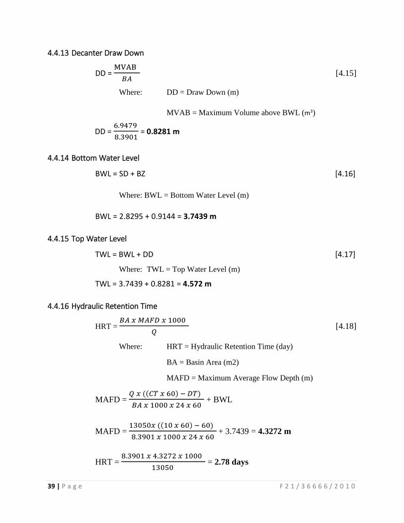
39 | P a g e F 2 1 / 3 6 6 6 6 / 2 0 1 0

4.4.13 Decanter Draw Down

DD = MVAB

𝐵𝐴 [4.15]

Where: DD = Draw Down (m)

MVAB = Maximum Volume above BWL (m3)

DD = 6.9479

8.3901 = 0.8281 m

4.4.14 Bottom Water Level

BWL = SD + BZ [4.16]

Where: BWL = Bottom Water Level (m)

BWL = 2.8295 + 0.9144 = 3.7439 m

4.4.15 Top Water Level

TWL = BWL + DD [4.17]

Where: TWL = Top Water Level (m)

TWL = 3.7439 + 0.8281 = 4.572 m

4.4.16 Hydraulic Retention Time

HRT = 𝐵𝐴 𝑥 𝑀𝐴𝐹𝐷 𝑥 1000

𝑄 [4.18]

Where: HRT = Hydraulic Retention Time (day)

BA = Basin Area (m2)

MAFD = Maximum Average Flow Depth (m)

MAFD = 𝑄 𝑥 ((𝐶𝑇 𝑥 60) − 𝐷𝑇)

𝐵𝐴 𝑥 1000 𝑥 24 𝑥 60 + BWL

MAFD = 13050𝑥 ((10 𝑥 60) − 60)

8.3901 𝑥 1000 𝑥 24 𝑥 60 + 3.7439 = 4.3272 m

HRT = 8.3901 𝑥 4.3272 𝑥 1000

13050 = 2.78 days

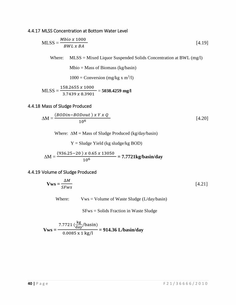
40 | P a g e F 2 1 / 3 6 6 6 6 / 2 0 1 0

4.4.17 MLSS Concentration at Bottom Water Level

MLSS = 𝑀𝑏𝑖𝑜 𝑥 1000

𝐵𝑊𝐿 𝑥 𝐵𝐴 [4.19]

Where: MLSS = Mixed Liquor Suspended Solids Concentration at BWL (mg/l)

Mbio = Mass of Biomass (kg/basin)

1000 = Conversion (mg/kg x m3/l)

MLSS = 158.2655 𝑥 1000

3.7439 𝑥 8.3901 = 5038.4259 mg/l

4.4.18 Mass of Sludge Produced

∆M = (𝐵𝑂𝐷𝑖𝑛−𝐵𝑂𝐷𝑜𝑢𝑡 ) 𝑥 𝑌 𝑥 𝑄

106 [4.20]

Where: ∆M = Mass of Sludge Produced (kg/day/basin)

Y = Sludge Yield (kg sludge/kg BOD)

∆M = (936.25−20 ) 𝑥 0.65 𝑥 13050

106 = 7.7721kg/basin/day

4.4.19 Volume of Sludge Produced

Vws = ∆𝑀

𝑆𝐹𝑤𝑠 [4.21]

Where: Vws = Volume of Waste Sludge (L/day/basin)

SFws = Solids Fraction in Waste Sludge

Vws =

7.7721 (kg

day/basin)

0.0085 x 1 kg/l = 914.36 L/basin/day

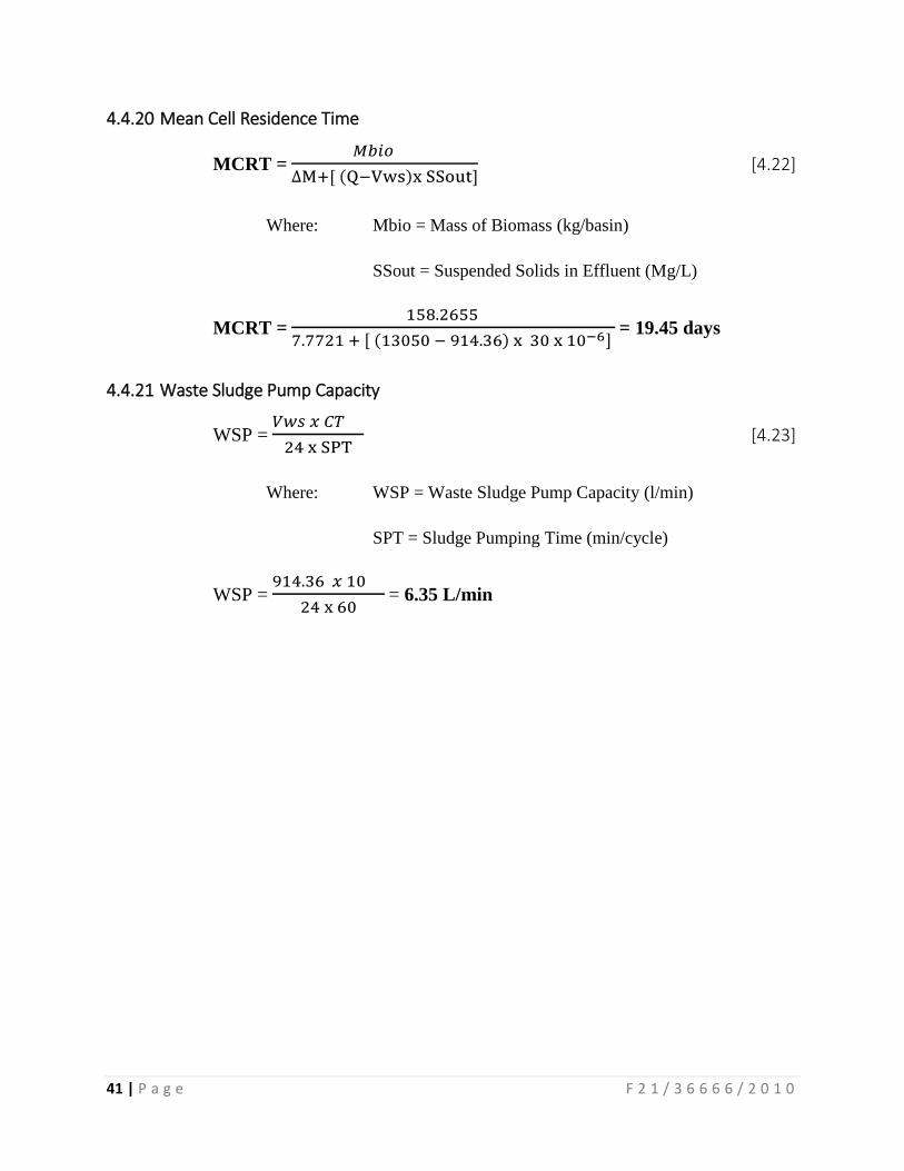
41 | P a g e F 2 1 / 3 6 6 6 6 / 2 0 1 0

4.4.20 Mean Cell Residence Time

MCRT = 𝑀𝑏𝑖𝑜

∆M+[ (Q−Vws)x SSout] [4.22]

Where: Mbio = Mass of Biomass (kg/basin)

SSout = Suspended Solids in Effluent (Mg/L)

MCRT = 158.2655

7.7721 + [ (13050 − 914.36) x 30 x 10−6] = 19.45 days

4.4.21 Waste Sludge Pump Capacity

WSP = 𝑉𝑤𝑠 𝑥 𝐶𝑇

24 x SPT [4.23]

Where: WSP = Waste Sludge Pump Capacity (l/min)

SPT = Sludge Pumping Time (min/cycle)

WSP = 914.36 𝑥 10

24 x 60 = 6.35 L/min

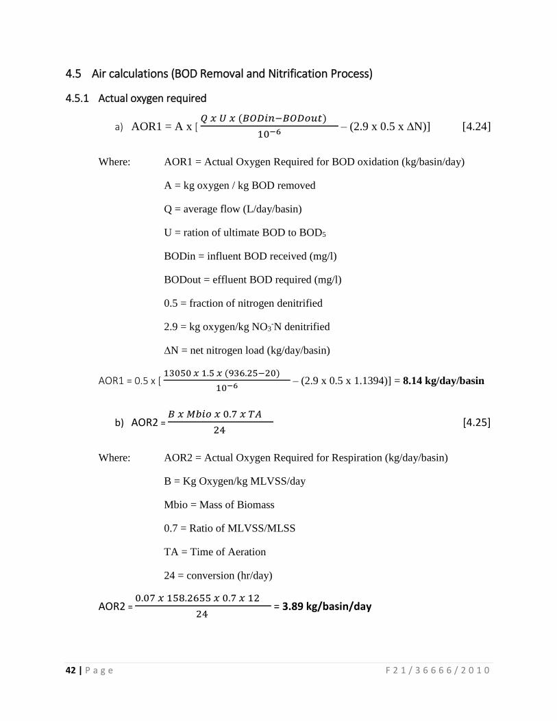
42 | P a g e F 2 1 / 3 6 6 6 6 / 2 0 1 0

4.5 Air calculations (BOD Removal and Nitrification Process)

4.5.1 Actual oxygen required

a) AOR1 = A x [ 𝑄 𝑥 𝑈 𝑥 (𝐵𝑂𝐷𝑖𝑛−𝐵𝑂𝐷𝑜𝑢𝑡)

10−6 – (2.9 x 0.5 x ∆N)] [4.24]

Where: AOR1 = Actual Oxygen Required for BOD oxidation (kg/basin/day)

A = kg oxygen / kg BOD removed

Q = average flow (L/day/basin)

U = ration of ultimate BOD to BOD5

BODin = influent BOD received (mg/l)

BODout = effluent BOD required (mg/l)

0.5 = fraction of nitrogen denitrified

2.9 = kg oxygen/kg NO3-N denitrified

∆N = net nitrogen load (kg/day/basin)

AOR1 = 0.5 x [ 13050 𝑥 1.5 𝑥 (936.25−20)

10−6 – (2.9 x 0.5 x 1.1394)] = 8.14 kg/day/basin

b) AOR2 = 𝐵 𝑥 𝑀𝑏𝑖𝑜 𝑥 0.7 𝑥 𝑇𝐴

24 [4.25]

Where: AOR2 = Actual Oxygen Required for Respiration (kg/day/basin)

B = Kg Oxygen/kg MLVSS/day

Mbio = Mass of Biomass

0.7 = Ratio of MLVSS/MLSS

TA = Time of Aeration

24 = conversion (hr/day)

AOR2 = 0.07 𝑥 158.2655 𝑥 0.7 𝑥 12

24 = 3.89 kg/basin/day

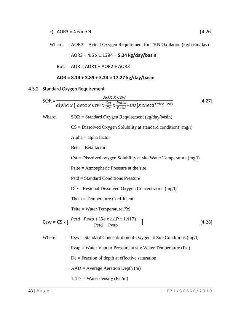
43 | P a g e F 2 1 / 3 6 6 6 6 / 2 0 1 0

c) AOR3 = 4.6 x ∆N [4.26]

Where: AOR3 = Actual Oxygen Requirement for TKN Oxidation (kg/basin/day)

AOR3 = 4.6 x 1.1394 = 5.24 kg/day/basin

But: AOR = AOR1 + AOR2 + AOR3

AOR = 8.14 + 3.89 + 5.24 = 17.27 kg/day/basin

4.5.2 Standard Oxygen Requirement

SOR = 𝐴𝑂𝑅 𝑥 𝐶𝑠𝑤

𝑎𝑙𝑝ℎ𝑎 𝑥 ( 𝑏𝑒𝑡𝑎 𝑥 𝐶𝑠𝑤 𝑥 𝐶𝑠𝑡

𝐶𝑠 𝑥

𝑃𝑠𝑖𝑡𝑒

𝑃𝑠𝑡𝑑−𝐷𝑂)𝑥 𝑡ℎ𝑒𝑡𝑎𝑇𝑠𝑖𝑡𝑒−20)

[4.27]

Where: SOR = Standard Oxygen Requirement (kg/day/basin)

CS = Dissolved Oxygen Solubility at standard conditions (mg/l)

Alpha = alpha factor

Beta = Beta factor

Cst = Dissolved oxygen Solubility at site Water Temperature (mg/l)

Psite = Atmospheric Pressure at the site

Pstd = Standard Conditions Pressure

DO = Residual Dissolved Oxygen Concentration (mg/l)

Theta = Temperature Coefficient

Tsite = Water Temperature (0c)

Csw = CS x [ 𝑃𝑠𝑡𝑑−𝑃𝑣𝑎𝑝 +(𝐷𝑒 𝑥 𝐴𝐴𝐷 𝑥 1,417)

Pstd − Pvap] [4.28]

Where: Csw = Standard Concentration of Oxygen at Site Conditions (mg/l)

Pvap = Water Vapour Pressure at site Water Temperature (Psi)

De = Fraction of depth at effective saturation

AAD = Average Aeration Depth (m)

1.417 = Water density (Psi/m)

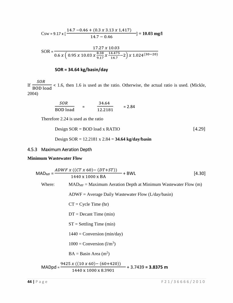
44 | P a g e F 2 1 / 3 6 6 6 6 / 2 0 1 0

Csw = 9.17 x [ 14.7 −0.46 + (0.3 𝑥 3.13 𝑥 1,417)

14.7 − 0.46] = 10.03 mg/l

SOR = 17.27 𝑥 10.03

0.6 𝑥 ( 0.95 𝑥 10.03 𝑥 8.38

9.17 𝑥

14.475

14.7−2) 𝑥 1.024(30−20)

SOR = 34.64 kg/basin/day

If 𝑆𝑂𝑅

BOD load < 1.6, then 1.6 is used as the ratio. Otherwise, the actual ratio is used. (Mickle,

2004)

𝑆𝑂𝑅

BOD load =

34.64

12.2181 = 2.84

Therefore 2.24 is used as the ratio

Design SOR = BOD load x RATIO [4.29]

Design SOR = 12.2181 x 2.84 = 34.64 kg/day/basin

4.5.3 Maximum Aeration Depth

Minimum Wastewater Flow

MADMF = 𝐴𝐷𝑊𝐹 𝑥 ((𝐶𝑇 𝑥 60)− (𝐷𝑇+𝑆𝑇))

1440 x 1000 x BA + BWL [4.30]

Where: MADMF = Maximum Aeration Depth at Minimum Wastewater Flow (m)

ADWF = Average Daily Wastewater Flow (L/day/basin)

CT = Cycle Time (hr)

DT = Decant Time (min)

ST = Settling Time (min)

1440 = Conversion (min/day)

1000 = Conversion (l/m3)

BA = Basin Area (m2)

MADpd = 9425 𝑥 ((10 𝑥 60)− (60+420))

1440 x 1000 x 8.3901 + 3.7439 = 3.8375 m

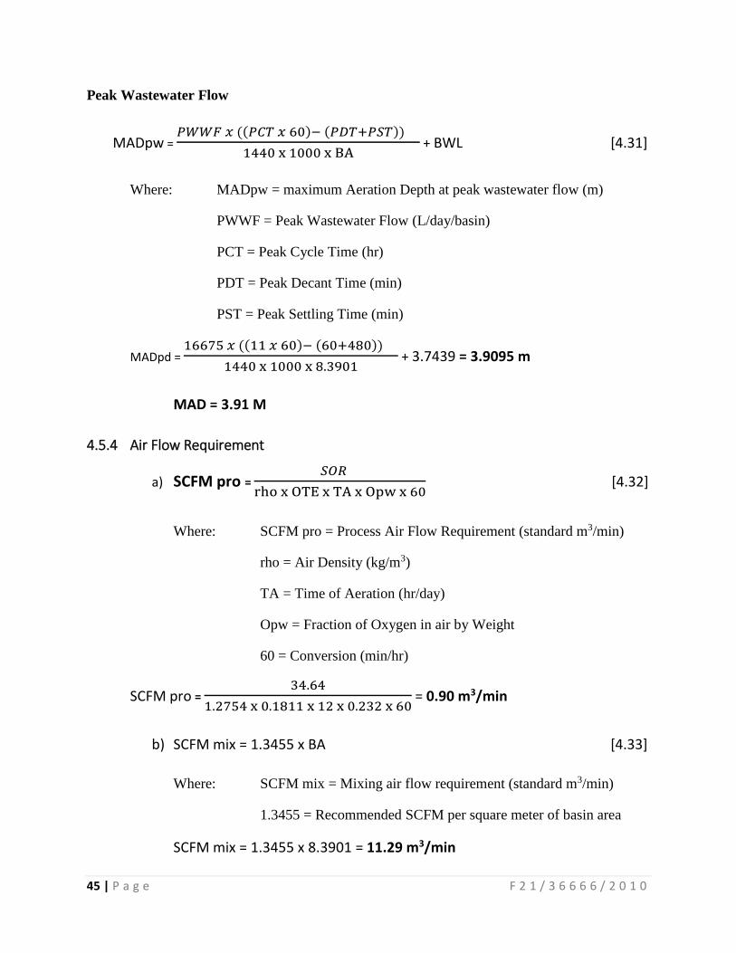
45 | P a g e F 2 1 / 3 6 6 6 6 / 2 0 1 0

Peak Wastewater Flow

MADpw = 𝑃𝑊𝑊𝐹 𝑥 ((𝑃𝐶𝑇 𝑥 60)− (𝑃𝐷𝑇+𝑃𝑆𝑇))

1440 x 1000 x BA + BWL [4.31]

Where: MADpw = maximum Aeration Depth at peak wastewater flow (m)

PWWF = Peak Wastewater Flow (L/day/basin)

PCT = Peak Cycle Time (hr)

PDT = Peak Decant Time (min)

PST = Peak Settling Time (min)

MADpd = 16675 𝑥 ((11 𝑥 60)− (60+480))

1440 x 1000 x 8.3901 + 3.7439 = 3.9095 m

MAD = 3.91 M

4.5.4 Air Flow Requirement

a) SCFM pro = 𝑆𝑂𝑅

rho x OTE x TA x Opw x 60 [4.32]

Where: SCFM pro = Process Air Flow Requirement (standard m3/min)

rho = Air Density (kg/m3)

TA = Time of Aeration (hr/day)

Opw = Fraction of Oxygen in air by Weight

60 = Conversion (min/hr)

SCFM pro = 34.64

1.2754 x 0.1811 x 12 x 0.232 x 60 = 0.90 m3/min

b) SCFM mix = 1.3455 x BA [4.33]

Where: SCFM mix = Mixing air flow requirement (standard m3/min)

1.3455 = Recommended SCFM per square meter of basin area

SCFM mix = 1.3455 x 8.3901 = 11.29 m3/min

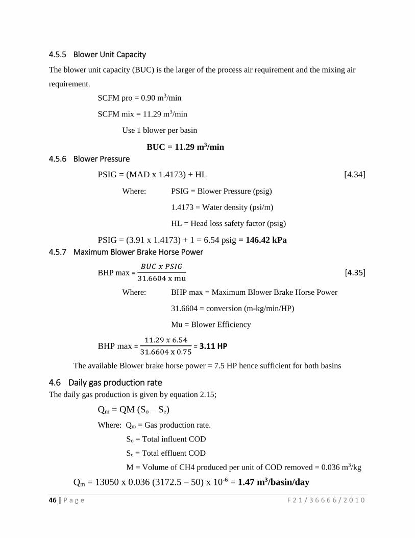
46 | P a g e F 2 1 / 3 6 6 6 6 / 2 0 1 0

4.5.5 Blower Unit Capacity

The blower unit capacity (BUC) is the larger of the process air requirement and the mixing air

requirement.

SCFM pro = 0.90 m3/min

SCFM mix = 11.29 m3/min

Use 1 blower per basin

BUC = 11.29 m3/min

4.5.6 Blower Pressure

PSIG = (MAD x 1.4173) + HL [4.34]

Where: PSIG = Blower Pressure (psig)

1.4173 = Water density (psi/m)

HL = Head loss safety factor (psig)

PSIG = (3.91 x 1.4173) + 1 = 6.54 psig = 146.42 kPa

4.5.7 Maximum Blower Brake Horse Power

BHP max = 𝐵𝑈𝐶 𝑥 𝑃𝑆𝐼𝐺

31.6604 x mu [4.35]

Where: BHP max = Maximum Blower Brake Horse Power

31.6604 = conversion (m-kg/min/HP)

Mu = Blower Efficiency

BHP max = 11.29 𝑥 6.54

31.6604 x 0.75 = 3.11 HP

The available Blower brake horse power = 7.5 HP hence sufficient for both basins

4.6 Daily gas production rate The daily gas production is given by equation 2.15;

Qm = QM (So – Se)

Where: Qm = Gas production rate.

So = Total influent COD

Se = Total effluent COD

M = Volume of CH4 produced per unit of COD removed = 0.036 m3/kg

Qm = 13050 x 0.036 (3172.5 – 50) x 10-6 = 1.47 m3/basin/day

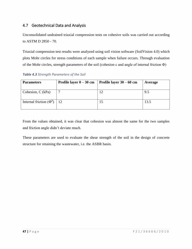
47 | P a g e F 2 1 / 3 6 6 6 6 / 2 0 1 0

4.7 Geotechnical Data and Analysis

Unconsolidated undrained triaxial compression tests on cohesive soils was carried out according

to ASTM D 2850 - 70.

Triaxial compression test results were analyzed using soil vision software (SoilVision 4.0) which

plots Mohr circles for stress conditions of each sample when failure occurs. Through evaluation

of the Mohr circles, strength parameters of the soil (cohesion c and angle of internal friction Ф)

Table 4.3 Strength Parameters of the Soil

Parameters Profile layer 0 – 30 cm Profile layer 30 – 60 cm Average

Cohesion, C (kPa) 7 12 9.5

Internal friction (Ф0) 12 15 13.5

From the values obtained, it was clear that cohesion was almost the same for the two samples

and friction angle didn’t deviate much.

These parameters are used to evaluate the shear strength of the soil in the design of concrete

structure for retaining the wastewater, i.e. the ASBR basin.

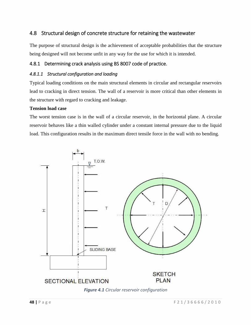
48 | P a g e F 2 1 / 3 6 6 6 6 / 2 0 1 0

4.8 Structural design of concrete structure for retaining the wastewater

The purpose of structural design is the achievement of acceptable probabilities that the structure

being designed will not become unfit in any way for the use for which it is intended.

4.8.1 Determining crack analysis using BS 8007 code of practice.

4.8.1.1 Structural configuration and loading

Typical loading conditions on the main structural elements in circular and rectangular reservoirs

lead to cracking in direct tension. The wall of a reservoir is more critical than other elements in

the structure with regard to cracking and leakage.

Tension load case

The worst tension case is in the wall of a circular reservoir, in the horizontal plane. A circular

reservoir behaves like a thin walled cylinder under a constant internal pressure due to the liquid

load. This configuration results in the maximum direct tensile force in the wall with no bending.

Figure 4.1 Circular reservoir configuration

49 | P a g e F 2 1 / 3 6 6 6 6 / 2 0 1 0

Design parameters

Table 4.4 Structural design parameters for concrete structure

Parameter Symbol Units

Concrete strength (concrete class) fcu 30 N/mm2

Concrete tensile strength (mean value) fct,eff 2.90 N/mm2

Reinforcement yield strength (characteristic value) fy 460 N/mm2

Modular ratio αe 15

Modulus of elasticity, steel Es 200 GPa

Density of water γw 9.81 kN/m3

The physical parameters of height of wall (H) thus liquid load (Lk), section thickness (h), cover

(c), the diameter (θ) and area of the tension reinforcement were chosen as follows:

1. A wall height of 5m, being reasonable for a reinforced concrete water retaining reservoir,

was chosen as the reference height for the analyses using BS 8007. The wall height of 5m

result in maximum service liquid loads of 50 kN/m2 and maximum ultimate liquid loads

(γ = 1.2) of 60 kN/m2 for the circular reservoir configurations.

2. Section thicknesses of 300 mm was considered for a wall height of 5m.

3. The reinforcement cover was taken as 40 mm as this is the value most commonly used in

practice for water retaining structures.

4. Bar diameter of 25 mm were considered as they are those typically used in reinforced

concrete water retaining structures. Diameters larger than 25 mm result in wider cracks

forming, while diameters smaller than 16 mm result in excessively small reinforcement

spacing’s.

5. In defining a representative range of reinforcement area (As), a maximum feasible limit

was determined by considering a minimum practical spacing of bars, namely, a 75 mm

spacing, given single reinforcing bars.

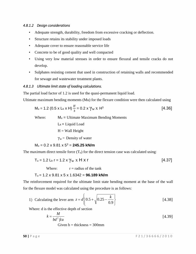
50 | P a g e F 2 1 / 3 6 6 6 6 / 2 0 1 0

4.8.1.2 Design considerations

• Adequate strength, durability, freedom from excessive cracking or deflection.

• Structure retains its stability under imposed loads

• Adequate cover to ensure reasonable service life

• Concrete to be of good quality and well compacted

• Using very low material stresses in order to ensure flexural and tensile cracks do not

develop.

• Sulphates resisting cement that used in construction of retaining walls and recommended

for sewage and wastewater treatment plants.

4.8.1.3 Ultimate limit state of loading calculations.

The partial load factor of 1.2 is used for the quasi-permanent liquid load.

Ultimate maximum bending moments (Mu) for the flexure condition were then calculated using

Mu = 1.2 (0.5 x Lk x H) 𝐻

3 = 0.2 x γw x H3 [4.36]

Where: Mu = Ultimate Maximum Bending Moments

Lk = Liquid Load

H = Wall Height

γw = Density of water

Mu = 0.2 x 9.81 x 53 = 245.25 kN/m

The maximum direct tensile force (Tu) for the direct tension case was calculated using:

Tu = 1.2 Lk r = 1.2 x γw x H x r [4.37]

Where: r = radius of the tank

Tu = 1.2 x 9.81 x 5 x 1.6342 = 96.189 kN/m

The reinforcement required for the ultimate limit state bending moment at the base of the wall

for the flexure model was calculated using the procedure is as follows:

1) Calculating the lever arm

9.0

25.05.0k

dz [4.38]

Where: d is the effective depth of section

fcubd

Mk

2 [4.39]

Given b = thickness = 300mm

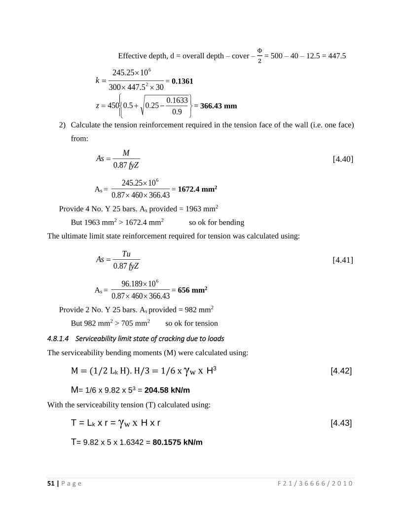
51 | P a g e F 2 1 / 3 6 6 6 6 / 2 0 1 0

Effective depth, d = overall depth – cover – Ф

2 = 500 – 40 – 12.5 = 447.5

305.447300

1025.245

2

6

k = 0.1361

9.0

1633.025.05.0450z = 366.43 mm

2) Calculate the tension reinforcement required in the tension face of the wall (i.e. one face)

from:

fyZ

MAs

87.0 [4.40]

As = 43.36646087.0

1025.245 6

= 1672.4 mm2

Provide 4 No. Y 25 bars. As provided = 1963 mm2

But 1963 mm2 > 1672.4 mm2 so ok for bending

The ultimate limit state reinforcement required for tension was calculated using:

fyZ

TuAs

87.0 [4.41]

As = 43.36646087.0

10189.96 6

= 656 mm2

Provide 2 No. Y 25 bars. As provided = 982 mm2

But 982 mm2 > 705 mm2 so ok for tension

4.8.1.4 Serviceability limit state of cracking due to loads

The serviceability bending moments (M) were calculated using:

M = (1/2 Lk H). H/3 = 1/6 x γw x H3 [4.42]

M= 1/6 x 9.82 x 53 = 204.58 kN/m

With the serviceability tension (T) calculated using:

T = Lk x r = γw x H x r [4.43]

T= 9.82 x 5 x 1.6342 = 80.1575 kN/m

52 | P a g e F 2 1 / 3 6 6 6 6 / 2 0 1 0

4.8.1.5 Assessment of crack widths in direct tension

The Serviceability limit state crack width, was then calculated using the relevant equations in

BS8007 code for a given reinforcement diameter and spacing, hence area of reinforcement, for

the tension crack conditions.

Stresses and strains were calculated using linear elastic theory. In the SLS tension cracking

model, a constant tensile stress distribution was assumed across the full thickness of the wall.

The procedures predicting the expected maximum crack width for a given wall geometry and

material properties are as follows:

1. Serviceability limit state tensile force

Given area provided As = 982 mm2, hence the design tensile force;

T = As x 0.87 x fy x Z [4.44]

T = 982 x 0.87 x 460 x 340.93 = 133.98 kN/m

2. Assumption:

Diameter of longitudinal bar = 25 mm

Center to center spacing of longitudinal bar = 75 mm

3. Distance from the crack to the nearest reinforcing bar (αcr) as for flexure.

222

2

min

2

c

sacr [4.45]

Where: = Diameter of longitudinal bar

Cmin = Minimum clear cover to the longitudinal bar

S = Center to center spacing of longitudinal bar

2

25

2

2520

2

7522

cra = 49.50 mm

4. Service steel stress, fs

fs = 𝑇

𝐴𝑠 [4.46]

fs = 133.98 𝑥 103

982 = 136.44 N/mm2

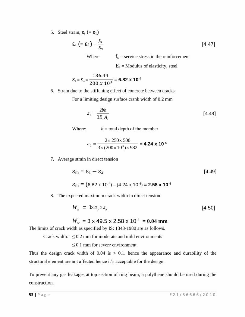
53 | P a g e F 2 1 / 3 6 6 6 6 / 2 0 1 0

5. Steel strain, εs (= ε1)

εs (= ε1) =.

𝑓𝑠

𝐸𝑠 [4.47]

Where: fs = service stress in the reinforcement

Es = Modulus of elasticity, steel

εs = ε1 = 136.44

200 𝑥 103 = 6.82 x 10-4

6. Strain due to the stiffening effect of concrete between cracks

For a limiting design surface crank width of 0.2 mm

ss AE

bh

3

22 [4.48]

Where: h = total depth of the member

982)10200(3

500250232

= 4.24 x 10-4

7. Average strain in direct tension

εm = ε1 – ε2 [4.49]

εm = (6.82 x 10-4) – (4.24 x 10-4) = 2.58 x 10-4

8. The expected maximum crack width in direct tension

crW = mcra 3 [4.50]

crW = 3 x 49.5 x 2.58 x 10-4 = 0.04 mm

The limits of crack width as specified by IS: 1343-1980 are as follows.

Crack width: ≤ 0.2 mm for moderate and mild environments

≤ 0.1 mm for severe environment.

Thus the design crack width of 0.04 is ≤ 0.1, hence the appearance and durability of the

structural element are not affected hence it’s acceptable for the design.

To prevent any gas leakages at top section of ring beam, a polythene should be used during the

construction.

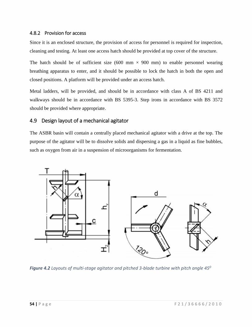
54 | P a g e F 2 1 / 3 6 6 6 6 / 2 0 1 0

4.8.2 Provision for access

Since it is an enclosed structure, the provision of access for personnel is required for inspection,

cleaning and testing. At least one access hatch should be provided at top cover of the structure.

The hatch should be of sufficient size (600 mm × 900 mm) to enable personnel wearing

breathing apparatus to enter, and it should be possible to lock the hatch in both the open and

closed positions. A platform will be provided under an access hatch.

Metal ladders, will be provided, and should be in accordance with class A of BS 4211 and

walkways should be in accordance with BS 5395-3. Step irons in accordance with BS 3572

should be provided where appropriate.

4.9 Design layout of a mechanical agitator

The ASBR basin will contain a centrally placed mechanical agitator with a drive at the top. The

purpose of the agitator will be to dissolve solids and dispersing a gas in a liquid as fine bubbles,

such as oxygen from air in a suspension of microorganisms for fermentation.

Figure 4.2 Layouts of multi-stage agitator and pitched 3-blade turbine with pitch angle 450

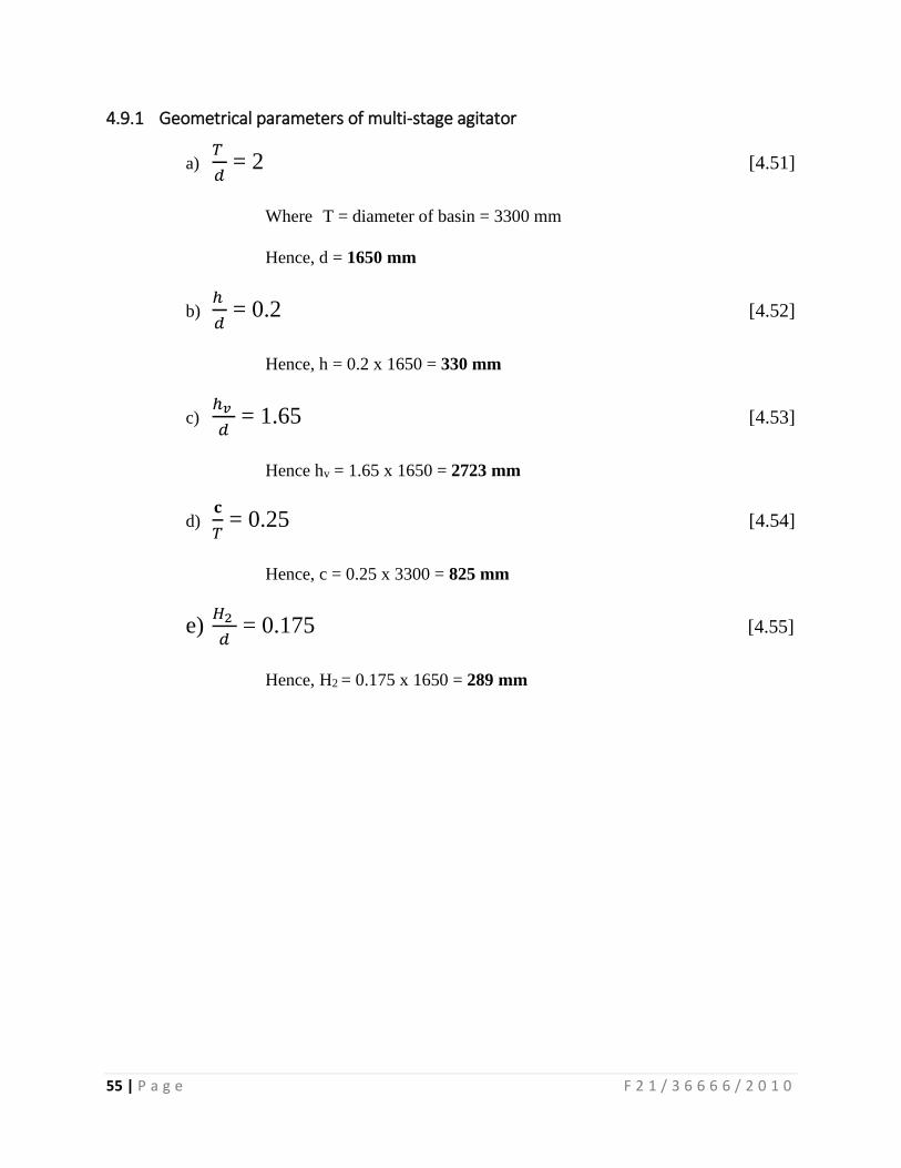
55 | P a g e F 2 1 / 3 6 6 6 6 / 2 0 1 0

4.9.1 Geometrical parameters of multi-stage agitator

a) 𝑇

𝑑 = 2 [4.51]

Where T = diameter of basin = 3300 mm

Hence, d = 1650 mm

b) ℎ

𝑑 = 0.2 [4.52]

Hence, h = 0.2 x 1650 = 330 mm

c) ℎ𝑣

𝑑 = 1.65 [4.53]

Hence hv = 1.65 x 1650 = 2723 mm

d) 𝐜

𝑇 = 0.25 [4.54]

Hence, c = 0.25 x 3300 = 825 mm

e) 𝐻2

𝑑 = 0.175 [4.55]

Hence, H2 = 0.175 x 1650 = 289 mm

56 | P a g e F 2 1 / 3 6 6 6 6 / 2 0 1 0

5 DISCUSSION

The design was done for two Anaerobic Sequencing Batch Reactor (ASBR) basins each with a

flow capacity of 16.68 m3/day. The Basin working volume of the ASBR was found to be 30.68

m3.The dimensions of the ASBR were found to be 3300 mm in diameter, a total height of 5570

mm and section thickness of 300 mm. The decanter size was obtained to be 300 mm with a

decanter rate of 127.38 l/min during peak hour. A top water level of 4572 mm was obtained

which is within the value specified in the design criteria.

The Hydraulic Retention Time, HRT was determined to be 2.78 days. This is ideal because a

long HRT is hypothesized to be beneficial for the start-up period because it might indirectly help

to increase the SRT of the system by preventing biomass washout and retaining the biomass in

the reactor. Ndon and Dague (1997) showed that anaerobic systems with short HRT have high

organic loading resulting in the domination of microorganisms which are more dispersed and

have a longer settling velocity which results in poor solid-liquid separation; and high hydraulic

loading which causes higher biomass loss in the effluent.

MLSS concentration at the bottom water level was obtained to be 5038.43 mg/l. With this result,

the ASBR showed its potential in operating at a high organic loading rate. Mass of sludge

produced per day is 7.77 kg/basin and Mean Cell Residence Time of 19.45 days. The daily gas

produced was calculated to be 1.47 m3/basin/day. By creating energy and reducing waste, ASBR is

both an appealing solution to common problems and an attractive investment.

The ASBR incorporates a blower with a Blower Unit Capacity of 11.29 m3/min, Blower pressure

of 146.42 Kpa and maximum blower brake horse power of 3.11 Hp. This will be sufficient to

provide a standard oxygen required of 34.64 kg/basin/day and can also achieve a maximum

aeration depth of 3910 mm. A multistage mechanical agitator with pitched 3-blade turbine is

incorporated at the center of the ASBR basin for dissolving solids and dispersing a gas in the liquid.

The structural design of the ASBR was achieved by determining the crack analysis using the BS

8007 code of practice. The crack width of 0.04 was obtained and since this crack width is less

than 0.1, the appearance and durability of the structural element were not affected since this is

within the limits of crack width as specified by IS: 1343-1980.

57 | P a g e F 2 1 / 3 6 6 6 6 / 2 0 1 0

The top cover of the ASBR was designed to have a fixed dome shape that is air tight so as to

improve/increase the pressure of the biogas in the reactor hence allowing the collection of daily

gas production. The cover has a provision for biogas line, pH dosing line, a mechanical agitator

and an access point of sufficient size (600 mm by 900 mm) for inspection, cleaning and testing.

58 | P a g e F 2 1 / 3 6 6 6 6 / 2 0 1 0

6 CONCLUSION

The overall objective of the project was achieved and the designer was able to come up with a

complete design of a wastewater treatment plant to be used for effective treatment of wastewater

from the slaughterhouse that can meet the effluent quality standards.

Wastewater samples and soil samples were collected. Wastewater content were determined

through lab tests and used to analyze the quantity and composition of slaughterhouse wastewater.

Pretreated wastewater was found to contain high levels of the waste content as indicated in table

4.1. Geotechnical data and analysis was carried out using triaxial compression test. The strength

parameters of the soil was determined, and cohesion was obtained to be 10 while internal friction

is 14. This data formed the basis of the design.

This design report shows a design of a properly sized Anaerobic Sequencing Batch Reactor

(ASBR) based on organic loading rates and hydraulic retention times derived from the analysis

of the quantity and composition of slaughterhouse wastewater. The sizing depend on the

discharge required, slope of the land, and available space. The ASBR system is presented in

AutoCAD drawings hence providing full visualization of its geometry, dimensions and materials.

The design uses relevant parameters (i.e. BOD, COD, TSS, TDS and NH4+N (N)) and has a

provision for desludging, access for sampling and inspection, leakage monitoring and security

provision and utilizes processes that require a minimum operation time.

The higher methane production 1.47 m3/basin/day at a lower HRT of 2.78 days also showed that

a higher organic loading rate was preferred by the anaerobic microorganisms. A reaction phase

of 120 min was used. This duration of the reaction phase gives the microorganisms more time to

convert the complex organic molecules to soluble monomer molecules. More suspended solids

are converted into soluble compounds during the longer HRT, thus reducing the Mixed Liquor

Suspended Solids (MLSS) and Mixed Liquor Volatile Suspended solids (MLVSS)

concentrations.

59 | P a g e F 2 1 / 3 6 6 6 6 / 2 0 1 0

7 RECOMMENDATIONS

This design project report has shown that the ASBR has the potential of treating slaughterhouse

wastewater. Therefore the following recommendations should be applied to the treatment system

in order to optimize it to improve its performance:

Increase the diameter of the basin: this helps to increase the basin area and thus reducing

the overall depth.

To improve the quality of the ASBR-treated effluent, aerobic post treatment should be

introduced to further remove suspended solids, organic and nutrients like nitrogen and

phosphorus

Reduce the amount of water used for general cleaning purposes. Proper detergents should

also be used.

Stock pen waste should be hauled away for use as organic fertilizer and the area cleaned

periodically with as little water as possible.

Regular monitoring and testing of the effluent should be done to ensure that the effluent

flowing into the wetland conforms to the NEMA standards.

60 | P a g e F 2 1 / 3 6 6 6 6 / 2 0 1 0

8 REFERENCES

Adelegan, J. A., (2002). Environmental policy and slaughterhouse waste in Nigeria. Proceedings

of the 28th WEDC Conference. Calcutta, India.

Akinro, A. O., Ologunagba, I.B., and Yahaya, O. (2009). Environmental implications of

unhygienic operation of a city abattoir in Akure, Western Nigeria. ARPN Journal of Engineering

and Applied Sciences; 4 (9): 311–315.

Alaerts, G. J., Veenstra, S., Bentvelsen, M., Lindfield, M., Specker, H., Van Velsen L.,

Wildschut, L., Lettinga, G., Hulshoff, P. L., and Zuidema, M. (1989). Assessment of the

feasibility of anaerobic sewage treatment in developing countries. Reports of the international

institute for hydraulic and environmental engineering, Delft, The Netherlands, 178.

Aniebo, A. O., Wekhe, S. N., and Okoli, I. C. (2009). “Abattoir blood waste generation in rivers

state and its environmental implications in the Niger Delta,” Toxicological and Environmental

Chemistry; 91: 619–625.

Bello, Y. O., and Oyedemi, D .T .A. (2009). Impact of abattoir activities and management in

residential neighborhoods: A case study of Ogbomoso, Nigeria. Journal of Social Science;

19:121–127.

BS 8007-1987. Code of practice for Design of Concrete Structures for retaining aqueous liquids.

British Standard

Chukwu, O. (2008). Analysis of groundwater pollution from abattoir Waste in Minna, Nigeria.

Research Journal of Diary Science; 2: 74–77.

Chynoweth, D. P., Owens, J., Legrand, R., and Glick, D. (1996). Renewable methane from

anaerobic digestion of biomass. The Seventh National Bioenergy, 96.

Eastman, J. A., and Ferguson, J. F. (1981). Solubilization of particulate organic carbon during

the acid phase of anaerobic digestion. Journal of Water Pollution Control Federation; 53: 6352-

6366.

Eikelboom, D. H., and van Buijsen, H. J. J. (1983). Microscopic sludge investigation manual.

Research Institute for Environmental Hygiene, Delft, Netherlands.

European Commission. (2005). Integrated Pollution Prevention and Control: Reference

Document on Best Available Techniques in the Slaughterhouses and Animal by-Products

Industries.

Gauri, S. M. (2006). Treatment of wastewater from abattoirs before land application: a review.

Bioresource Technology; 97 (9): 1119–1135.

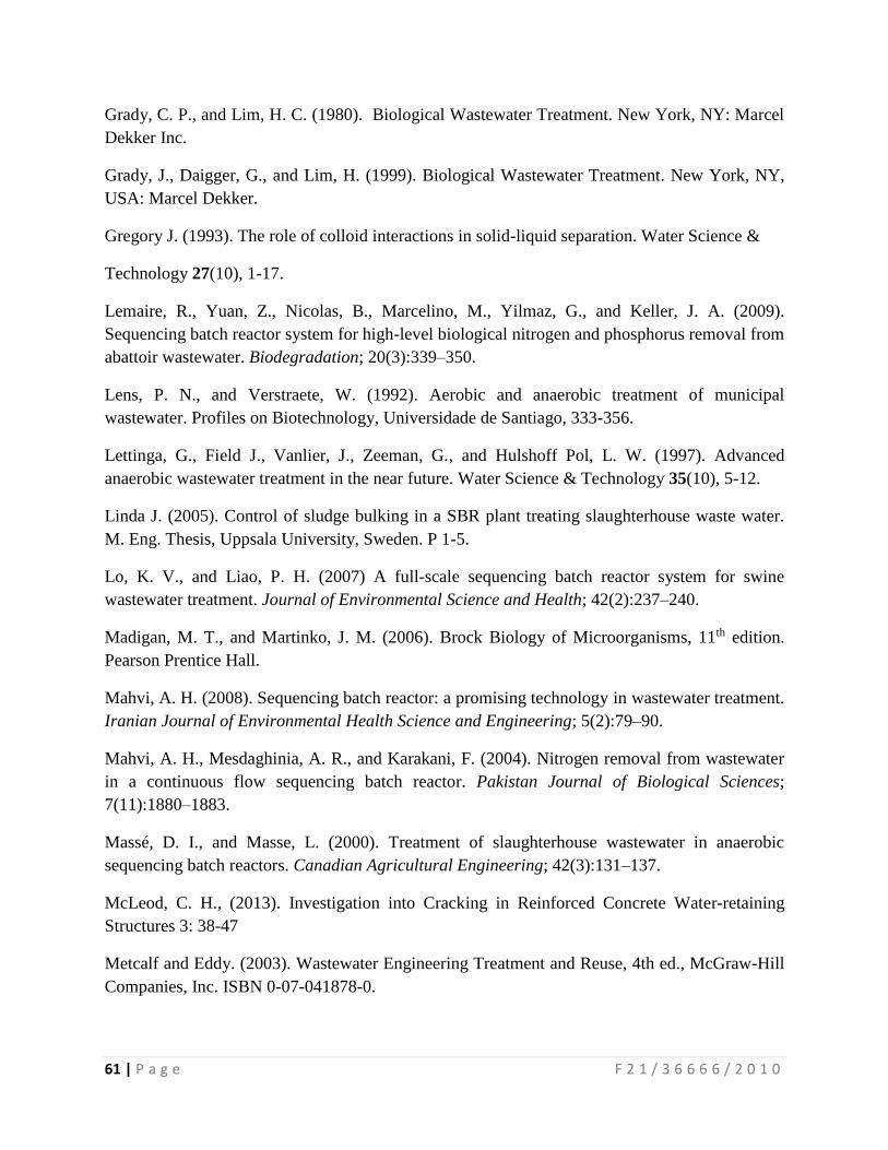
61 | P a g e F 2 1 / 3 6 6 6 6 / 2 0 1 0

Grady, C. P., and Lim, H. C. (1980). Biological Wastewater Treatment. New York, NY: Marcel

Dekker Inc.

Grady, J., Daigger, G., and Lim, H. (1999). Biological Wastewater Treatment. New York, NY,

USA: Marcel Dekker.

Gregory J. (1993). The role of colloid interactions in solid-liquid separation. Water Science &

Technology 27(10), 1-17.

Lemaire, R., Yuan, Z., Nicolas, B., Marcelino, M., Yilmaz, G., and Keller, J. A. (2009).

Sequencing batch reactor system for high-level biological nitrogen and phosphorus removal from

abattoir wastewater. Biodegradation; 20(3):339–350.

Lens, P. N., and Verstraete, W. (1992). Aerobic and anaerobic treatment of municipal

wastewater. Profiles on Biotechnology, Universidade de Santiago, 333-356.

Lettinga, G., Field J., Vanlier, J., Zeeman, G., and Hulshoff Pol, L. W. (1997). Advanced

anaerobic wastewater treatment in the near future. Water Science & Technology 35(10), 5-12.

Linda J. (2005). Control of sludge bulking in a SBR plant treating slaughterhouse waste water.

M. Eng. Thesis, Uppsala University, Sweden. P 1-5.

Lo, K. V., and Liao, P. H. (2007) A full-scale sequencing batch reactor system for swine

wastewater treatment. Journal of Environmental Science and Health; 42(2):237–240.

Madigan, M. T., and Martinko, J. M. (2006). Brock Biology of Microorganisms, 11th edition.

Pearson Prentice Hall.

Mahvi, A. H. (2008). Sequencing batch reactor: a promising technology in wastewater treatment.

Iranian Journal of Environmental Health Science and Engineering; 5(2):79–90.

Mahvi, A. H., Mesdaghinia, A. R., and Karakani, F. (2004). Nitrogen removal from wastewater

in a continuous flow sequencing batch reactor. Pakistan Journal of Biological Sciences;

7(11):1880–1883.

Massé, D. I., and Masse, L. (2000). Treatment of slaughterhouse wastewater in anaerobic

sequencing batch reactors. Canadian Agricultural Engineering; 42(3):131–137.

McLeod, C. H., (2013). Investigation into Cracking in Reinforced Concrete Water-retaining

Structures 3: 38-47

Metcalf and Eddy. (2003). Wastewater Engineering Treatment and Reuse, 4th ed., McGraw-Hill

Companies, Inc. ISBN 0-07-041878-0.

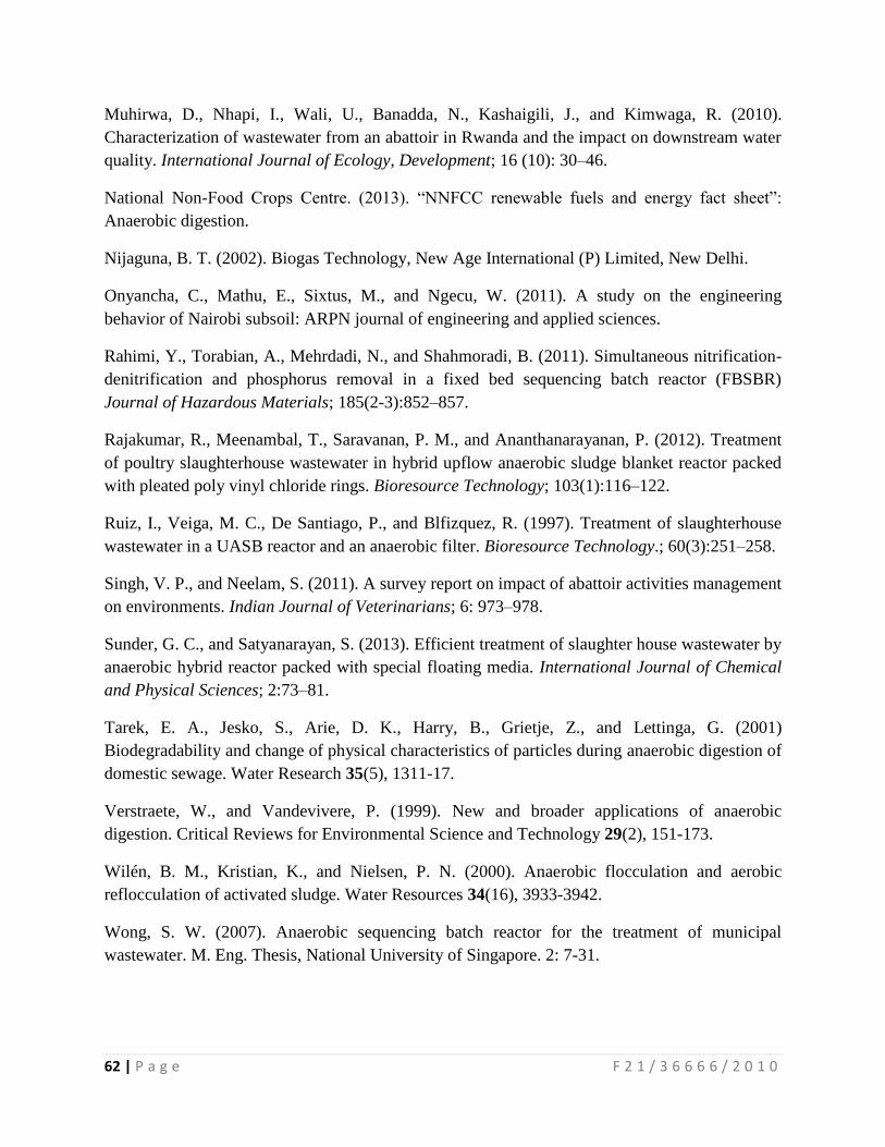
62 | P a g e F 2 1 / 3 6 6 6 6 / 2 0 1 0

Muhirwa, D., Nhapi, I., Wali, U., Banadda, N., Kashaigili, J., and Kimwaga, R. (2010).

Characterization of wastewater from an abattoir in Rwanda and the impact on downstream water

quality. International Journal of Ecology, Development; 16 (10): 30–46.

National Non-Food Crops Centre. (2013). “NNFCC renewable fuels and energy fact sheet”:

Anaerobic digestion.

Nijaguna, B. T. (2002). Biogas Technology, New Age International (P) Limited, New Delhi.

Onyancha, C., Mathu, E., Sixtus, M., and Ngecu, W. (2011). A study on the engineering

behavior of Nairobi subsoil: ARPN journal of engineering and applied sciences.

Rahimi, Y., Torabian, A., Mehrdadi, N., and Shahmoradi, B. (2011). Simultaneous nitrification-

denitrification and phosphorus removal in a fixed bed sequencing batch reactor (FBSBR)

Journal of Hazardous Materials; 185(2-3):852–857.

Rajakumar, R., Meenambal, T., Saravanan, P. M., and Ananthanarayanan, P. (2012). Treatment

of poultry slaughterhouse wastewater in hybrid upflow anaerobic sludge blanket reactor packed

with pleated poly vinyl chloride rings. Bioresource Technology; 103(1):116–122.

Ruiz, I., Veiga, M. C., De Santiago, P., and Blfizquez, R. (1997). Treatment of slaughterhouse

wastewater in a UASB reactor and an anaerobic filter. Bioresource Technology.; 60(3):251–258.

Singh, V. P., and Neelam, S. (2011). A survey report on impact of abattoir activities management

on environments. Indian Journal of Veterinarians; 6: 973–978.

Sunder, G. C., and Satyanarayan, S. (2013). Efficient treatment of slaughter house wastewater by

anaerobic hybrid reactor packed with special floating media. International Journal of Chemical

and Physical Sciences; 2:73–81.

Tarek, E. A., Jesko, S., Arie, D. K., Harry, B., Grietje, Z., and Lettinga, G. (2001)

Biodegradability and change of physical characteristics of particles during anaerobic digestion of

domestic sewage. Water Research 35(5), 1311-17.

Verstraete, W., and Vandevivere, P. (1999). New and broader applications of anaerobic

digestion. Critical Reviews for Environmental Science and Technology 29(2), 151-173.

Wilén, B. M., Kristian, K., and Nielsen, P. N. (2000). Anaerobic flocculation and aerobic

reflocculation of activated sludge. Water Resources 34(16), 3933-3942.

Wong, S. W. (2007). Anaerobic sequencing batch reactor for the treatment of municipal

wastewater. M. Eng. Thesis, National University of Singapore. 2: 7-31.

63 | P a g e F 2 1 / 3 6 6 6 6 / 2 0 1 0

9 APPENDICES

9.1 Appendix A: Site Photographs

Figure 9.1 Source of waste inform of blood as a result of slaughtering

Figure 9.2 Floor showing waste generated during slaughtering

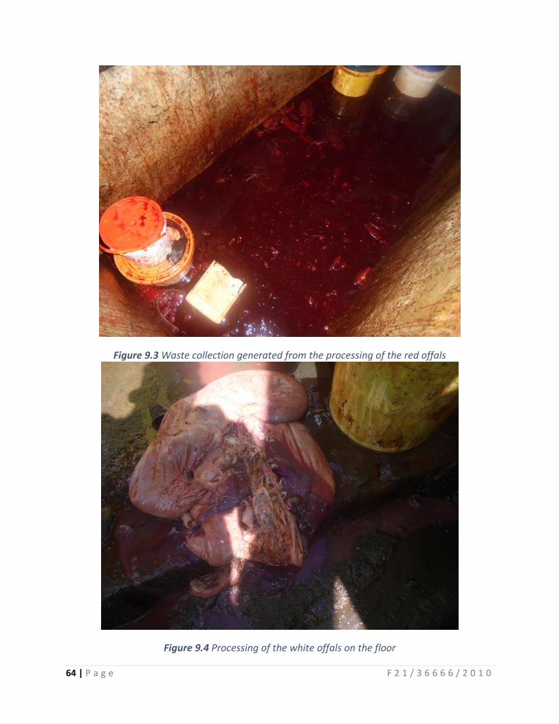
64 | P a g e F 2 1 / 3 6 6 6 6 / 2 0 1 0

Figure 9.3 Waste collection generated from the processing of the red offals

Figure 9.4 Processing of the white offals on the floor

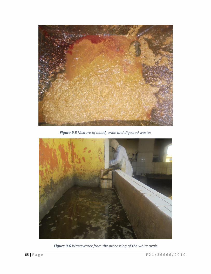
65 | P a g e F 2 1 / 3 6 6 6 6 / 2 0 1 0

Figure 9.5 Mixture of blood, urine and digested wastes

Figure 9.6 Wastewater from the processing of the white ovals

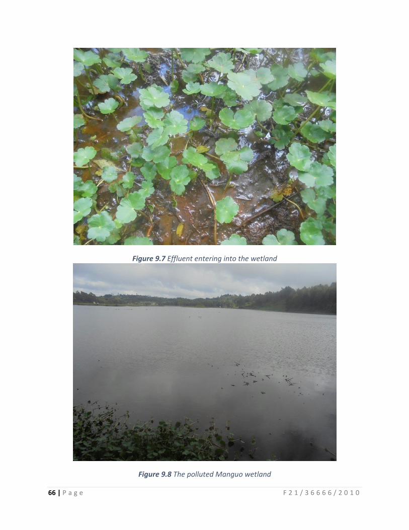
66 | P a g e F 2 1 / 3 6 6 6 6 / 2 0 1 0

Figure 9.7 Effluent entering into the wetland

Figure 9.8 The polluted Manguo wetland

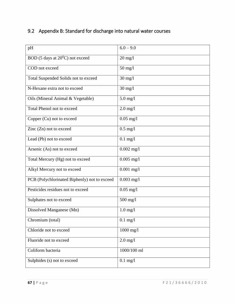
67 | P a g e F 2 1 / 3 6 6 6 6 / 2 0 1 0

9.2 Appendix B: Standard for discharge into natural water courses

pH 6.0 – 9.0

BOD (5 days at 200C) not exceed 20 mg/l

COD not exceed 50 mg/l

Total Suspended Solids not to exceed 30 mg/l

N-Hexane extra not to exceed 30 mg/l

Oils (Mineral Animal & Vegetable) 5.0 mg/l

Total Phenol not to exceed 2.0 mg/l

Copper (Cu) not to exceed 0.05 mg/l

Zinc (Zn) not to exceed 0.5 mg/l

Lead (Pb) not to exceed 0.1 mg/l

Arsenic (As) not to exceed 0.002 mg/l

Total Mercury (Hg) not to exceed 0.005 mg/l

Alkyl Mercury not to exceed 0.001 mg/l

PCB (Polychlorinated Biphenly) not to exceed 0.003 mg/l

Pesticides residues not to exceed 0.05 mg/l

Sulphates not to exceed 500 mg/l

Dissolved Manganese (Mn) 1.0 mg/l

Chromium (total) 0.1 mg/l

Chloride not to exceed 1000 mg/l

Fluoride not to exceed 2.0 mg/l

Coliform bacteria 1000/100 ml

Sulphides (s) not to exceed 0.1 mg/l

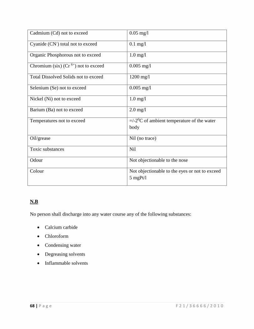
68 | P a g e F 2 1 / 3 6 6 6 6 / 2 0 1 0

Cadmium (Cd) not to exceed 0.05 mg/l

Cyanide (CN-) total not to exceed 0.1 mg/l

Organic Phosphorous not to exceed 1.0 mg/l

Chromium (six) (Cr 6+) not to exceed 0.005 mg/l

Total Dissolved Solids not to exceed 1200 mg/l

Selenium (Se) not to exceed 0.005 mg/l

Nickel (Ni) not to exceed 1.0 mg/l

Barium (Ba) not to exceed 2.0 mg/l

Temperatures not to exceed =/-20C of ambient temperature of the water

body

Oil/grease Nil (no trace)

Toxic substances Nil

Odour Not objectionable to the nose

Colour Not objectionable to the eyes or not to exceed

5 mgPt/l

N.B

No person shall discharge into any water course any of the following substances:

Calcium carbide

Chloroform

Condensing water

Degreasing solvents

Inflammable solvents

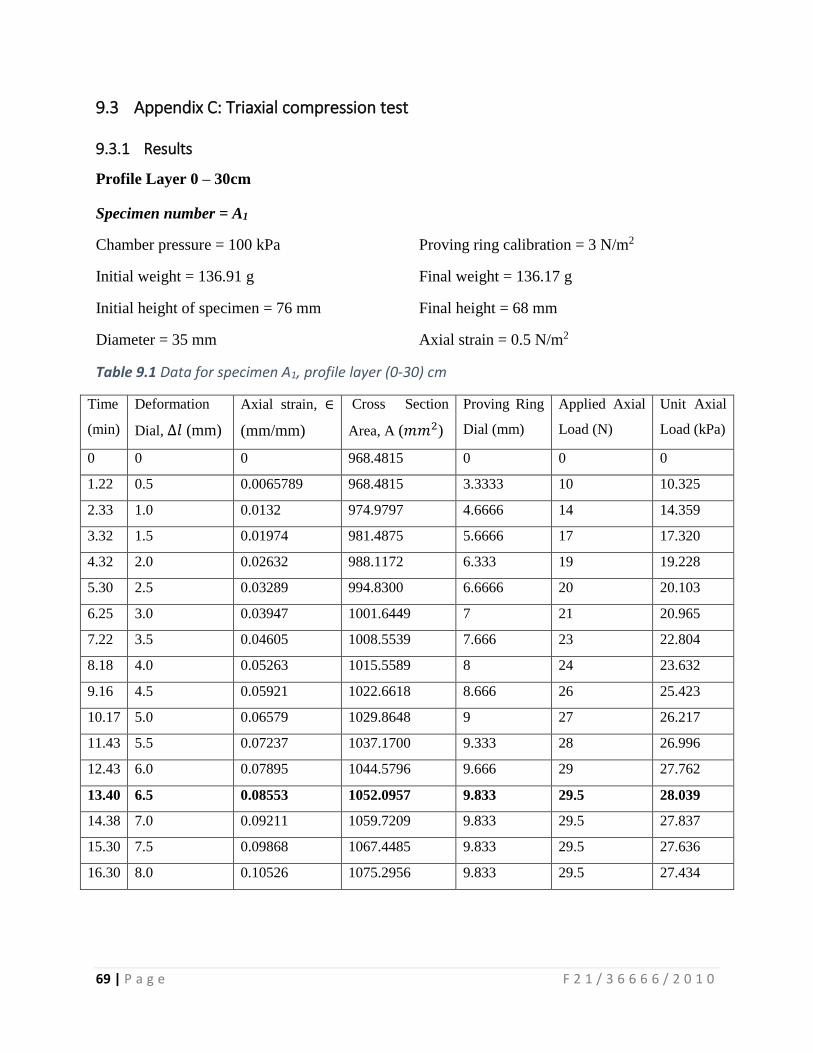
69 | P a g e F 2 1 / 3 6 6 6 6 / 2 0 1 0

9.3 Appendix C: Triaxial compression test

9.3.1 Results

Profile Layer 0 – 30cm

Specimen number = A1

Chamber pressure = 100 kPa Proving ring calibration = 3 N/m2

Initial weight = 136.91 g Final weight = 136.17 g

Initial height of specimen = 76 mm Final height = 68 mm

Diameter = 35 mm Axial strain = 0.5 N/m2

Table 9.1 Data for specimen A1, profile layer (0-30) cm

Time

(min)

Deformation

Dial, ∆𝑙 (mm)

Axial strain, ∈

(mm/mm)

Cross Section

Area, A (𝑚𝑚2)

Proving Ring

Dial (mm)

Applied Axial

Load (N)

Unit Axial

Load (kPa)

0 0 0 968.4815 0 0 0

1.22 0.5 0.0065789 968.4815 3.3333 10 10.325

2.33 1.0 0.0132 974.9797 4.6666 14 14.359

3.32 1.5 0.01974 981.4875 5.6666 17 17.320

4.32 2.0 0.02632 988.1172 6.333 19 19.228

5.30 2.5 0.03289 994.8300 6.6666 20 20.103

6.25 3.0 0.03947 1001.6449 7 21 20.965

7.22 3.5 0.04605 1008.5539 7.666 23 22.804

8.18 4.0 0.05263 1015.5589 8 24 23.632

9.16 4.5 0.05921 1022.6618 8.666 26 25.423

10.17 5.0 0.06579 1029.8648 9 27 26.217

11.43 5.5 0.07237 1037.1700 9.333 28 26.996

12.43 6.0 0.07895 1044.5796 9.666 29 27.762

13.40 6.5 0.08553 1052.0957 9.833 29.5 28.039

14.38 7.0 0.09211 1059.7209 9.833 29.5 27.837

15.30 7.5 0.09868 1067.4485 9.833 29.5 27.636

16.30 8.0 0.10526 1075.2956 9.833 29.5 27.434

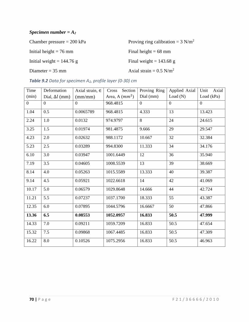
70 | P a g e F 2 1 / 3 6 6 6 6 / 2 0 1 0

Specimen number = A2

Chamber pressure = 200 kPa Proving ring calibration = 3 N/m2

Initial height = 76 mm Final height = 68 mm

Initial weight = 144.76 g Final weight = 143.68 g

Diameter = 35 mm Axial strain = 0.5 N/m2

Table 9.2 Data for specimen A2, profile layer (0-30) cm

Time

(min)

Deformation

Dial, ∆𝑙 (mm)

Axial strain, ∈

(mm/mm)

Cross Section

Area, A (𝑚𝑚2)

Proving Ring

Dial (mm)

Applied Axial

Load (N)

Unit Axial

Load (kPa)

0 0 0 968.4815 0 0 0

1.04 0.5 0.0065789 968.4815 4.333 13 13.423

2.24 1.0 0.0132 974.9797 8 24 24.615

3.25 1.5 0.01974 981.4875 9.666 29 29.547

4.23 2.0 0.02632 988.1172 10.667 32 32.384

5.23 2.5 0.03289 994.8300 11.333 34 34.176

6.10 3.0 0.03947 1001.6449 12 36 35.940

7.19 3.5 0.04605 1008.5539 13 39 38.669

8.14 4.0 0.05263 1015.5589 13.333 40 39.387

9.14 4.5 0.05921 1022.6618 14 42 41.069

10.17 5.0 0.06579 1029.8648 14.666 44 42.724

11.21 5.5 0.07237 1037.1700 18.333 55 43.387

12.35 6.0 0.07895 1044.5796 16.6667 50 47.866

13.36 6.5 0.08553 1052.0957 16.833 50.5 47.999

14.33 7.0 0.09211 1059.7209 16.833 50.5 47.654

15.32 7.5 0.09868 1067.4485 16.833 50.5 47.309

16.22 8.0 0.10526 1075.2956 16.833 50.5 46.963

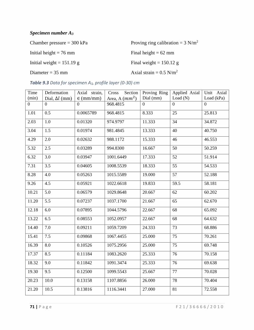
71 | P a g e F 2 1 / 3 6 6 6 6 / 2 0 1 0

Specimen number A3

Chamber pressure = 300 kPa Proving ring calibration = 3 N/m2

Initial height = 76 mm Final height = 62 mm

Initial weight = 151.19 g Final weight = 150.12 g

Diameter = 35 mm Axial strain = 0.5 N/m2

Table 9.3 Data for specimen A3, profile layer (0-30) cm

Time

(min)

Deformation

Dial, ∆𝑙 (mm)

Axial strain,

∈ (mm/mm) Cross Section

Area, A (𝑚𝑚2)

Proving Ring

Dial (mm)

Applied Axial

Load (N)

Unit Axial

Load (kPa)

0 0 0 968.4815 0 0 0

1.01 0.5 0.0065789 968.4815 8.333 25 25.813

2.03 1.0 0.01320 974.9797 11.333 34 34.872

3.04 1.5 0.01974 981.4845 13.333 40 40.750

4.29 2.0 0.02632 988.1172 15.333 46 46.553

5.32 2.5 0.03289 994.8300 16.667 50 50.259

6.32 3.0 0.03947 1001.6449 17.333 52 51.914

7.31 3.5 0.04605 1008.5539 18.333 55 54.533

8.28 4.0 0.05263 1015.5589 19.000 57 52.188

9.26 4.5 0.05921 1022.6618 19.833 59.5 58.181

10.21 5.0 0.06579 1029.8648 20.667 62 60.202

11.20 5.5 0.07237 1037.1700 21.667 65 62.670

12.18 6.0 0.07895 1044.5796 22.667 68 65.092

13.22 6.5 0.08553 1052.0957 22.667 68 64.632

14.40 7.0 0.09211 1059.7209 24.333 73 68.886

15.41 7.5 0.09868 1067.4455 25.000 75 70.261

16.39 8.0 0.10526 1075.2956 25.000 75 69.748

17.37 8.5 0.11184 1083.2620 25.333 76 70.158

18.32 9.0 0.11842 1091.3474 25.333 76 69.638

19.30 9.5 0.12500 1099.5543 25.667 77 70.028

20.23 10.0 0.13158 1107.8856 26.000 78 70.404

21.20 10.5 0.13816 1116.3441 27.000 81 72.558

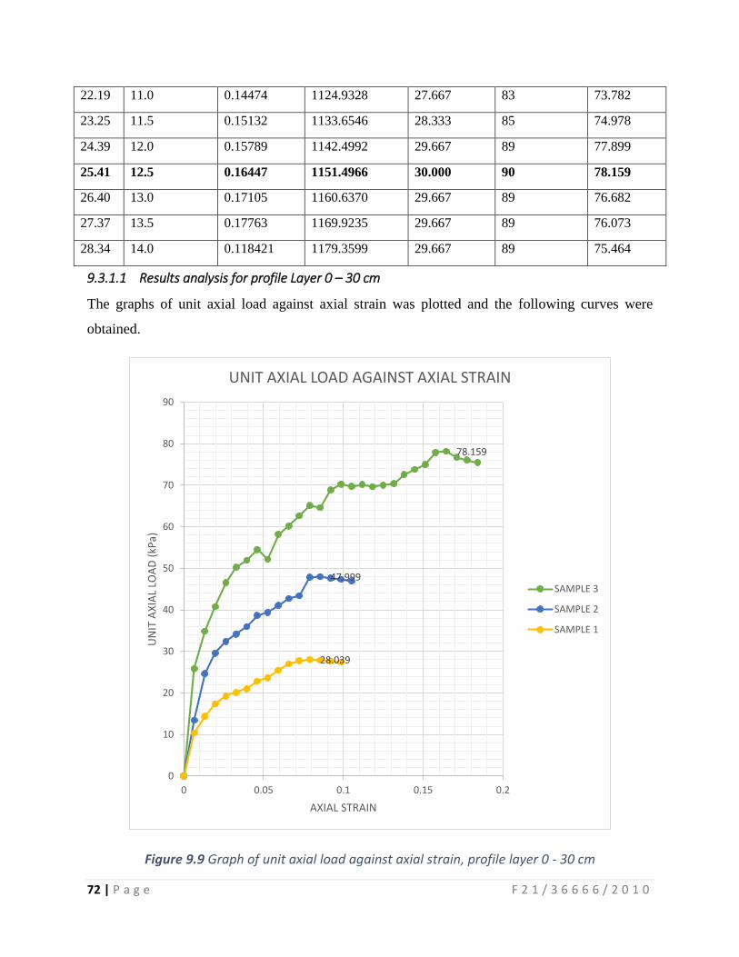
72 | P a g e F 2 1 / 3 6 6 6 6 / 2 0 1 0

22.19 11.0 0.14474 1124.9328 27.667 83 73.782

23.25 11.5 0.15132 1133.6546 28.333 85 74.978

24.39 12.0 0.15789 1142.4992 29.667 89 77.899

25.41 12.5 0.16447 1151.4966 30.000 90 78.159

26.40 13.0 0.17105 1160.6370 29.667 89 76.682

27.37 13.5 0.17763 1169.9235 29.667 89 76.073

28.34 14.0 0.118421 1179.3599 29.667 89 75.464

9.3.1.1 Results analysis for profile Layer 0 – 30 cm

The graphs of unit axial load against axial strain was plotted and the following curves were

obtained.

Figure 9.9 Graph of unit axial load against axial strain, profile layer 0 - 30 cm

78.159

47.999

28.039

0

10

20

30

40

50

60

70

80

90

0 0.05 0.1 0.15 0.2

UN

IT A

XIA

L LO

AD

(kP

a)

AXIAL STRAIN

UNIT AXIAL LOAD AGAINST AXIAL STRAIN

SAMPLE 3

SAMPLE 2

SAMPLE 1

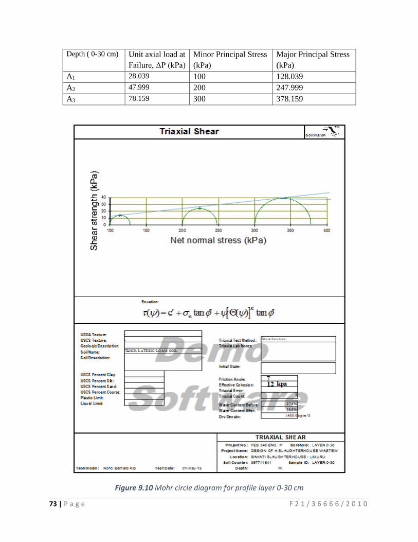
73 | P a g e F 2 1 / 3 6 6 6 6 / 2 0 1 0

Depth ( 0-30 cm) Unit axial load at

Failure, ΔP (kPa)

Minor Principal Stress

(kPa)

Major Principal Stress

(kPa)

A1 28.039 100 128.039

A2 47.999 200 247.999

A3 78.159 300 378.159

Figure 9.10 Mohr circle diagram for profile layer 0-30 cm

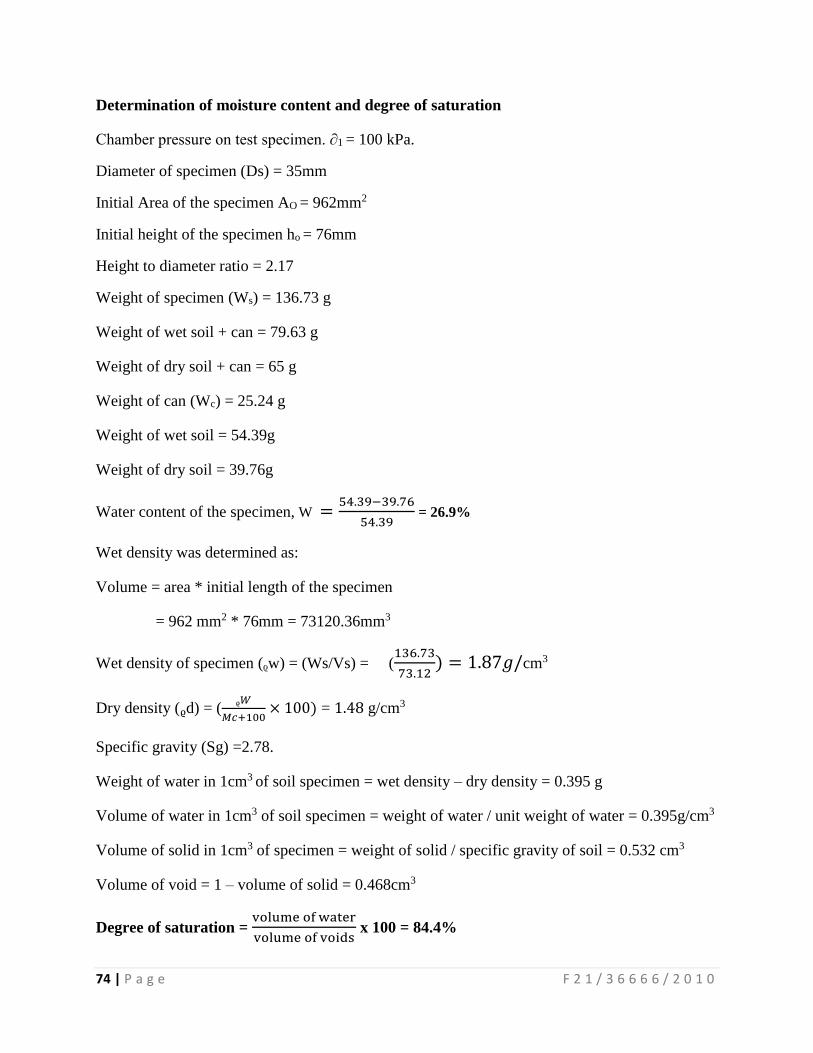
74 | P a g e F 2 1 / 3 6 6 6 6 / 2 0 1 0

Determination of moisture content and degree of saturation

Chamber pressure on test specimen. ∂1 = 100 kPa.

Diameter of specimen (Ds) = 35mm

Initial Area of the specimen AO = 962mm2

Initial height of the specimen ho = 76mm

Height to diameter ratio = 2.17

Weight of specimen (Ws) = 136.73 g

Weight of wet soil + can = 79.63 g

Weight of dry soil + can = 65 g

Weight of can (Wc) = 25.24 g

Weight of wet soil = 54.39g

Weight of dry soil = 39.76g

Water content of the specimen, W =54.39−39.76

54.39 = 26.9%

Wet density was determined as:

Volume = area * initial length of the specimen

= 962 mm2 * 76mm = 73120.36mm3

Wet density of specimen (ᵨw) = (Ws/Vs) = (136.73

73.12) = 1.87𝑔/cm3

Dry density (ᵨd) = (ᵨ𝑊

𝑀𝑐+100× 100) = 1.48 g/cm3

Specific gravity (Sg) =2.78.

Weight of water in 1cm3 of soil specimen = wet density – dry density = 0.395 g

Volume of water in 1cm3 of soil specimen = weight of water / unit weight of water = 0.395g/cm3

Volume of solid in 1cm3 of specimen = weight of solid / specific gravity of soil = 0.532 cm3

Volume of void = 1 – volume of solid = 0.468cm3

Degree of saturation = volume of water

volume of voids x 100 = 84.4%

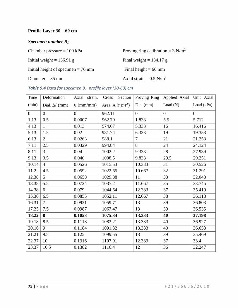
75 | P a g e F 2 1 / 3 6 6 6 6 / 2 0 1 0

Profile Layer 30 – 60 cm

Specimen number B1

Chamber pressure = 100 kPa Proving ring calibration = 3 N/m2

Initial weight = 136.91 g Final weight = 134.17 g

Initial height of specimen = 76 mm Final height = 66 mm

Diameter = 35 mm Axial strain = 0.5 N/m2

Table 9.4 Data for specimen B1, profile layer (30-60) cm

Time

(min)

Deformation

Dial, ∆𝑙 (mm)

Axial strain,

∈ (mm/mm)

Cross Section

Area, A (𝑚𝑚2)

Proving Ring

Dial (mm)

Applied Axial

Load (N)

Unit Axial

Load (kPa)

0 0 0 962.11 0 0 0

1.13 0.5 0.0007 962.79 1.833 5.5 5.712

4.13 1 0.013 974.67 5.333 16 16.416

5.13 1.5 0.02 981.74 6.333 19 19.353

6.13 2 0.0263 988.1 7 21 21.253

7.11 2.5 0.0329 994.84 8 24 24.124

8.11 3 0.04 1002.2 9.333 28 27.939

9.13 3.5 0.046 1008.5 9.833 29.5 29.251

10.14 4 0.0526 1015.53 10.333 31 30.526

11.2 4.5 0.0592 1022.65 10.667 32 31.291

12.38 5 0.0658 1029.88 11 33 32.043

13.38 5.5 0.0724 1037.2 11.667 35 33.745

14.38 6 0.079 1044.64 12.333 37 35.419

15.36 6.5 0.0855 1052.11 12.667 38 36.118

16.31 7 0.0921 1059.71 13 39 36.803

17.25 7.5 0.0987 1067.47 13 39 36.535

18.22 8 0.1053 1075.34 13.333 40 37.198

19.18 8.5 0.1118 1083.21 13.333 40 36.927

20.16 9 0.1184 1091.32 13.333 40 36.653

21.21 9.5 0.125 1099.55 13 39 35.469

22.37 10 0.1316 1107.91 12.333 37 33.4

23.37 10.5 0.1382 1116.4 12 36 32.247

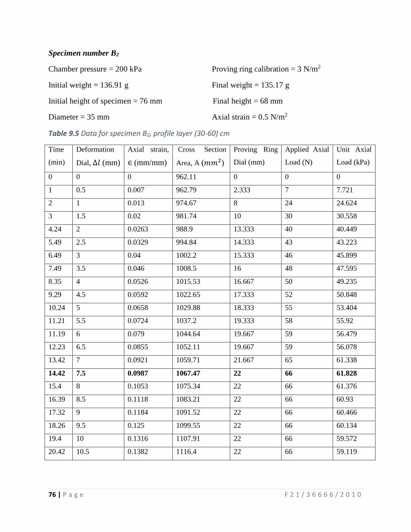
76 | P a g e F 2 1 / 3 6 6 6 6 / 2 0 1 0

Specimen number B2

Chamber pressure = 200 kPa Proving ring calibration = 3 N/m2

Initial weight = 136.91 g Final weight = 135.17 g

Initial height of specimen = 76 mm Final height = 68 mm

Diameter = 35 mm Axial strain = 0.5 N/m2

Table 9.5 Data for specimen B2, profile layer (30-60) cm

Time

(min)

Deformation

Dial, ∆𝑙 (mm)

Axial strain,

∈ (mm/mm)

Cross Section

Area, A (𝑚𝑚2)

Proving Ring

Dial (mm)

Applied Axial

Load (N)

Unit Axial

Load (kPa)

0 0 0 962.11 0 0 0

1 0.5 0.007 962.79 2.333 7 7.721

2 1 0.013 974.67 8 24 24.624

3 1.5 0.02 981.74 10 30 30.558

4.24 2 0.0263 988.9 13.333 40 40.449

5.49 2.5 0.0329 994.84 14.333 43 43.223

6.49 3 0.04 1002.2 15.333 46 45.899

7.49 3.5 0.046 1008.5 16 48 47.595

8.35 4 0.0526 1015.53 16.667 50 49.235

9.29 4.5 0.0592 1022.65 17.333 52 50.848

10.24 5 0.0658 1029.88 18.333 55 53.404

11.21 5.5 0.0724 1037.2 19.333 58 55.92

11.19 6 0.079 1044.64 19.667 59 56.479

12.23 6.5 0.0855 1052.11 19.667 59 56.078

13.42 7 0.0921 1059.71 21.667 65 61.338

14.42 7.5 0.0987 1067.47 22 66 61.828

15.4 8 0.1053 1075.34 22 66 61.376

16.39 8.5 0.1118 1083.21 22 66 60.93

17.32 9 0.1184 1091.52 22 66 60.466

18.26 9.5 0.125 1099.55 22 66 60.134

19.4 10 0.1316 1107.91 22 66 59.572

20.42 10.5 0.1382 1116.4 22 66 59.119

77 | P a g e F 2 1 / 3 6 6 6 6 / 2 0 1 0

Specimen number B3

Chamber pressure = 300 kPa Proving ring calibration = 3 N/m2

Initial weight = 116.979 g Final weight = 104.12 g

Initial height of specimen = 76 mm Final height = 64 mm

Diameter = 35 mm Axial strain = 0.5 N/m2

Table 9.6 Data for specimen B3, profile layer (30-60) cm Time

(min)

Deformation

Dial, ∆𝑙 (mm)

Axial strain,

∈ (mm/mm)

Cross Section

Area, A (m𝑚2)

Proving Ring

Dial (mm)

Applied Axial

Load (N)

Unit Axial

Load (kPa)

0 0 0 962.11 0 0 0

1.2 0.5 0.0007 962.79 3.667 11 11.425

2.2 1 0.013 974.67 6.333 19 19.494

2.57 1.5 0.02 981.74 7.667 23 23.428

3.56 2 0.0263 988.1 9 27 27.325

5.22 2.5 0.0329 994.84 10 30 30.156

12.41 3 0.04 1002.2 10.667 32 31.93

20.43 3.5 0.042 1004.29 10.667 32 31.863

9.3.1.2 Results analysis for profile Layer 30 – 60 cm

Figure 9.11 Graph of unit axial load against axial strain, profile layer 30 – 60 cm

0

10

20

30

40

50

60

70

-0.02 0 0.02 0.04 0.06 0.08 0.1 0.12 0.14 0.16

Unit Axial Load

Axial Strain

Graph of unit axial load against axial strain

Sample 1

Sample 2

Sample 3

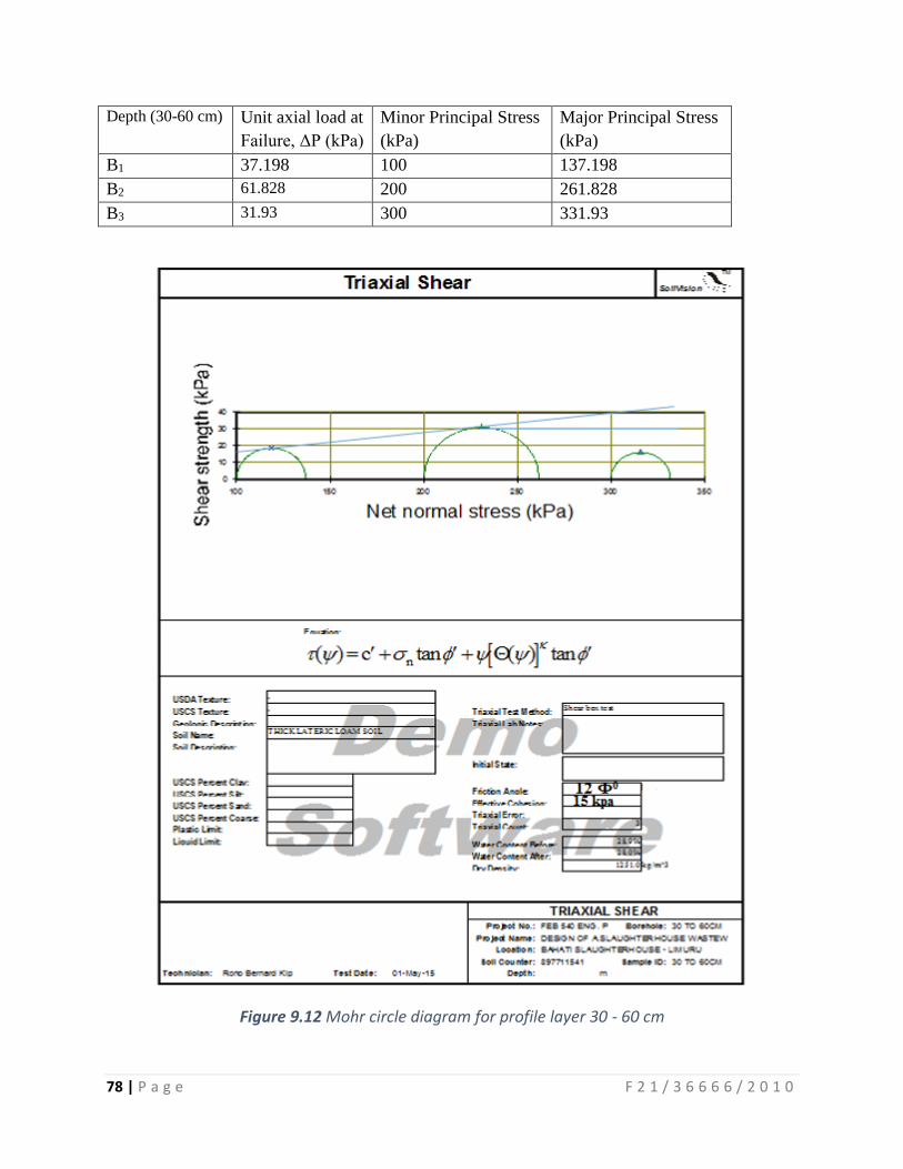
78 | P a g e F 2 1 / 3 6 6 6 6 / 2 0 1 0

Depth (30-60 cm) Unit axial load at

Failure, ΔP (kPa)

Minor Principal Stress

(kPa)

Major Principal Stress

(kPa)

B1 37.198 100 137.198

B2 61.828 200 261.828

B3 31.93 300 331.93

Figure 9.12 Mohr circle diagram for profile layer 30 - 60 cm

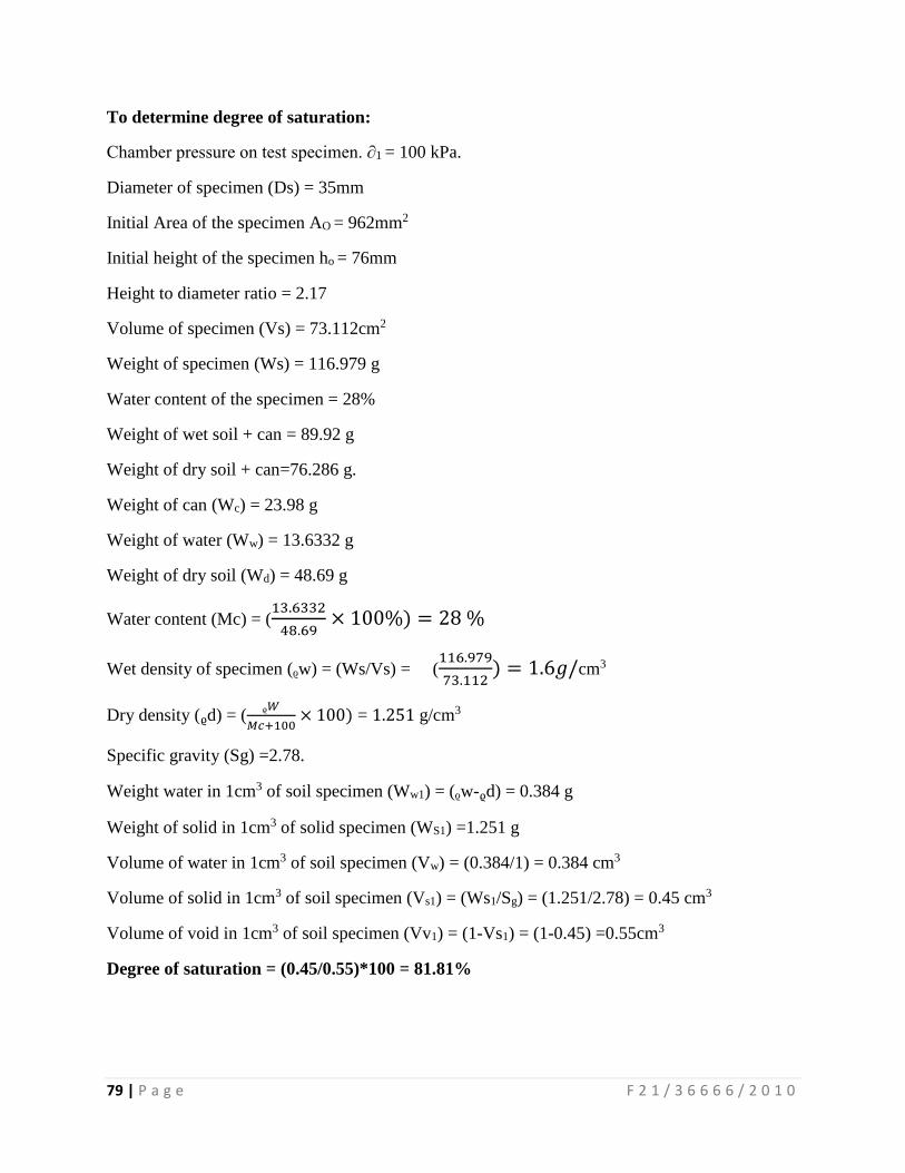
79 | P a g e F 2 1 / 3 6 6 6 6 / 2 0 1 0

To determine degree of saturation:

Chamber pressure on test specimen. ∂1 = 100 kPa.

Diameter of specimen (Ds) = 35mm

Initial Area of the specimen AO = 962mm2

Initial height of the specimen ho = 76mm

Height to diameter ratio = 2.17

Volume of specimen (Vs) = 73.112cm2

Weight of specimen (Ws) = 116.979 g

Water content of the specimen = 28%

Weight of wet soil + can = 89.92 g

Weight of dry soil + can=76.286 g.

Weight of can (Wc) = 23.98 g

Weight of water (Ww) = 13.6332 g

Weight of dry soil (Wd) = 48.69 g

Water content (Mc) = (13.6332

48.69× 100%) = 28 %

Wet density of specimen (ᵨw) = (Ws/Vs) = (116.979

73.112) = 1.6𝑔/cm3

Dry density (ᵨd) = (ᵨ𝑊

𝑀𝑐+100× 100) = 1.251 g/cm3

Specific gravity (Sg) =2.78.

Weight water in 1cm3 of soil specimen (Ww1) = (ᵨw-ᵨd) = 0.384 g

Weight of solid in 1cm3 of solid specimen (WS1) =1.251 g

Volume of water in 1cm3 of soil specimen (Vw) = (0.384/1) = 0.384 cm3

Volume of solid in 1cm3 of soil specimen (Vs1) = (Ws1/Sg) = (1.251/2.78) = 0.45 cm3

Volume of void in 1cm3 of soil specimen (Vv1) = (1-Vs1) = (1-0.45) =0.55cm3

Degree of saturation = (0.45/0.55)*100 = 81.81%

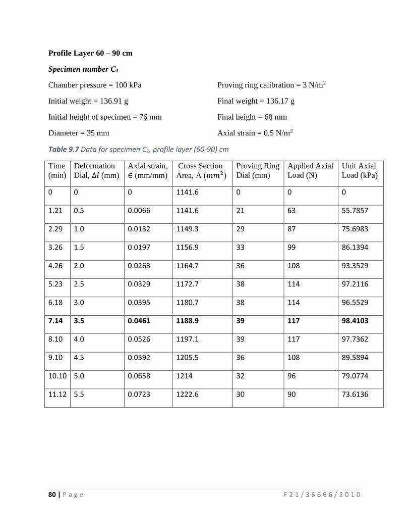
80 | P a g e F 2 1 / 3 6 6 6 6 / 2 0 1 0

Profile Layer 60 – 90 cm

Specimen number C1

Chamber pressure = 100 kPa Proving ring calibration = 3 N/m2

Initial weight = 136.91 g Final weight = 136.17 g

Initial height of specimen = 76 mm Final height = 68 mm

Diameter = 35 mm Axial strain = 0.5 N/m2

Table 9.7 Data for specimen C1, profile layer (60-90) cm

Time

(min)

Deformation

Dial, ∆𝑙 (mm)

Axial strain,

∈ (mm/mm)

Cross Section

Area, A (𝑚𝑚2)

Proving Ring

Dial (mm)

Applied Axial

Load (N)

Unit Axial

Load (kPa)

0 0 0 1141.6 0 0 0

1.21 0.5 0.0066 1141.6 21 63 55.7857

2.29 1.0 0.0132 1149.3 29 87 75.6983

3.26 1.5 0.0197 1156.9 33 99 86.1394

4.26 2.0 0.0263 1164.7 36 108 93.3529

5.23 2.5 0.0329 1172.7 38 114 97.2116

6.18 3.0 0.0395 1180.7 38 114 96.5529

7.14 3.5 0.0461 1188.9 39 117 98.4103

8.10 4.0 0.0526 1197.1 39 117 97.7362

9.10 4.5 0.0592 1205.5 36 108 89.5894

10.10 5.0 0.0658 1214 32 96 79.0774

11.12 5.5 0.0723 1222.6 30 90 73.6136

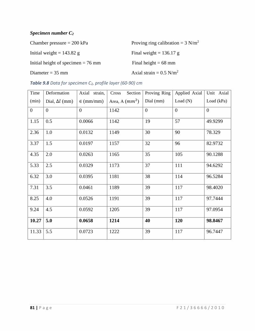
81 | P a g e F 2 1 / 3 6 6 6 6 / 2 0 1 0

Specimen number C2

Chamber pressure = 200 kPa Proving ring calibration = 3 N/m2

Initial weight = 143.82 g Final weight = 136.17 g

Initial height of specimen = 76 mm Final height = 68 mm

Diameter = 35 mm Axial strain = 0.5 N/m2

Table 9.8 Data for specimen C2, profile layer (60-90) cm

Time

(min)

Deformation

Dial, ∆𝑙 (mm)

Axial strain,

∈ (mm/mm)

Cross Section

Area, A (𝑚𝑚2)

Proving Ring

Dial (mm)

Applied Axial

Load (N)

Unit Axial

Load (kPa)

0 0 0 1142 0 0 0

1.15 0.5 0.0066 1142 19 57 49.9299

2.36 1.0 0.0132 1149 30 90 78.329

3.37 1.5 0.0197 1157 32 96 82.9732

4.35 2.0 0.0263 1165 35 105 90.1288

5.33 2.5 0.0329 1173 37 111 94.6292

6.32 3.0 0.0395 1181 38 114 96.5284

7.31 3.5 0.0461 1189 39 117 98.4020

8.25 4.0 0.0526 1191 39 117 97.7444

9.24 4.5 0.0592 1205 39 117 97.0954

10.27 5.0 0.0658 1214 40 120 98.8467

11.33 5.5 0.0723 1222 39 117 96.7447

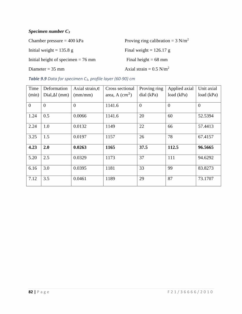
82 | P a g e F 2 1 / 3 6 6 6 6 / 2 0 1 0

Specimen number C3

Chamber pressure = 400 kPa Proving ring calibration = 3 N/m2

Initial weight = 135.8 g Final weight = 126.17 g

Initial height of specimen = 76 mm Final height = 68 mm

Diameter = 35 mm Axial strain = 0.5 N/m2

Table 9.9 Data for specimen C3, profile layer (60-90) cm

Time

(min)

Deformation

Dial,∆𝑙 (mm)

Axial strain,∈

(mm/mm)

Cross sectional

area, A (c𝑚2)

Proving ring

dial (kPa)

Applied axial

load (kPa)

Unit axial

load (kPa)

0 0 0 1141.6 0 0 0

1.24 0.5 0.0066 1141.6 20 60 52.5394

2.24 1.0 0.0132 1149 22 66 57.4413

3.25 1.5 0.0197 1157 26 78 67.4157

4.23 2.0 0.0263 1165 37.5 112.5 96.5665

5.20 2.5 0.0329 1173 37 111 94.6292

6.16 3.0 0.0395 1181 33 99 83.8273

7.12 3.5 0.0461 1189 29 87 73.1707

83 | P a g e F 2 1 / 3 6 6 6 6 / 2 0 1 0

9.3.1.3 Results analysis for profile Layer 60 – 90 cm

Figure 9.13 Graph of unit axial load against axial strain, profile layer 60 – 90 cm

0

20

40

60

80

100

120

0 0.01 0.02 0.03 0.04 0.05 0.06 0.07 0.08

Un

it A

xial

Lo

ad

Axial Strain

Graph of Unit Axial Load against Axial stain

Sample 1

Sample 2

Sample 3

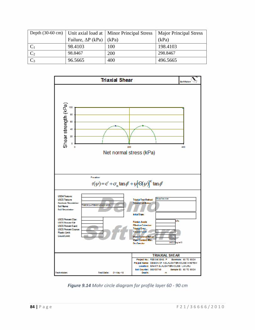
84 | P a g e F 2 1 / 3 6 6 6 6 / 2 0 1 0

Depth (30-60 cm) Unit axial load at

Failure, ΔP (kPa)

Minor Principal Stress

(kPa)

Major Principal Stress

(kPa)

C1 98.4103 100 198.4103

C2 98.8467 200 298.8467

C3 96.5665 400 496.5665

Figure 9.14 Mohr circle diagram for profile layer 60 - 90 cm

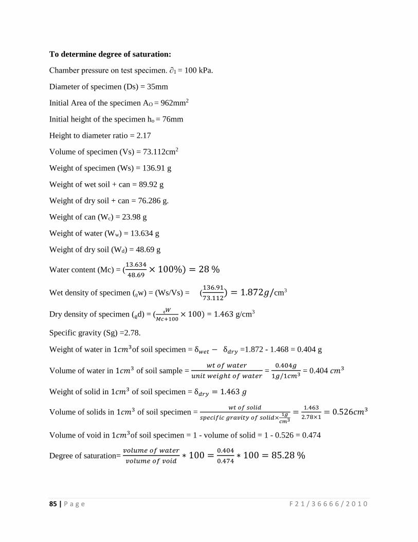
85 | P a g e F 2 1 / 3 6 6 6 6 / 2 0 1 0

To determine degree of saturation:

Chamber pressure on test specimen. ∂1 = 100 kPa.

Diameter of specimen (Ds) = 35mm

Initial Area of the specimen AO = 962mm2

Initial height of the specimen ho = 76mm

Height to diameter ratio = 2.17

Volume of specimen (Vs) = 73.112cm2

Weight of specimen (Ws) = 136.91 g

Weight of wet soil + can = 89.92 g

Weight of dry soil + can = 76.286 g.

Weight of can (Wc) = 23.98 g

Weight of water (Ww) = 13.634 g

Weight of dry soil (Wd) = 48.69 g

Water content (Mc) = (13.634

48.69× 100%) = 28 %

Wet density of specimen (ᵨw) = (Ws/Vs) = (136.91

73.112) = 1.872𝑔/cm3

Dry density of specimen (ᵨd) = (ᵨ𝑊

𝑀𝑐+100× 100) = 1.463 g/cm3

Specific gravity (Sg) =2.78.

Weight of water in 1𝑐𝑚3of soil specimen = δ𝑤𝑒𝑡 − δ𝑑𝑟𝑦 =1.872 - 1.468 = 0.404 g

Volume of water in 1𝑐𝑚3 of soil sample = 𝑤𝑡 𝑜𝑓 𝑤𝑎𝑡𝑒𝑟

𝑢𝑛𝑖𝑡 𝑤𝑒𝑖𝑔ℎ𝑡 𝑜𝑓 𝑤𝑎𝑡𝑒𝑟 =

0.404𝑔

1𝑔/1𝑐𝑚3 = 0.404 𝑐𝑚3

Weight of solid in 1𝑐𝑚3 of soil specimen = δ𝑑𝑟𝑦 = 1.463 𝑔

Volume of solids in 1𝑐𝑚3 of soil specimen = 𝑤𝑡 𝑜𝑓 𝑠𝑜𝑙𝑖𝑑

𝑠𝑝𝑒𝑐𝑖𝑓𝑖𝑐 𝑔𝑟𝑎𝑣𝑖𝑡𝑦 𝑜𝑓 𝑠𝑜𝑙𝑖𝑑×1𝑔

𝑐𝑚3

=1.463

2.78×1= 0.526𝑐𝑚3

Volume of void in 1𝑐𝑚3of soil specimen = 1 - volume of solid = 1 - 0.526 = 0.474

Degree of saturation= 𝑣𝑜𝑙𝑢𝑚𝑒 𝑜𝑓 𝑤𝑎𝑡𝑒𝑟

𝑣𝑜𝑙𝑢𝑚𝑒 𝑜𝑓 𝑣𝑜𝑖𝑑∗ 100 =

0.404

0.474∗ 100 = 85.28 %

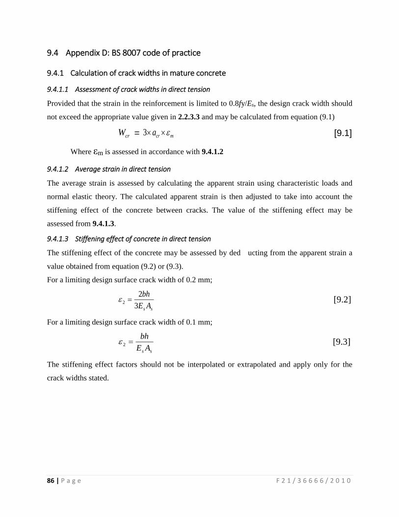
86 | P a g e F 2 1 / 3 6 6 6 6 / 2 0 1 0

9.4 Appendix D: BS 8007 code of practice

9.4.1 Calculation of crack widths in mature concrete

9.4.1.1 Assessment of crack widths in direct tension

Provided that the strain in the reinforcement is limited to 0.8fy/Es, the design crack width should

not exceed the appropriate value given in 2.2.3.3 and may be calculated from equation (9.1)

crW = mcra 3 [9.1]

Where εm is assessed in accordance with 9.4.1.2

9.4.1.2 Average strain in direct tension

The average strain is assessed by calculating the apparent strain using characteristic loads and

normal elastic theory. The calculated apparent strain is then adjusted to take into account the

stiffening effect of the concrete between cracks. The value of the stiffening effect may be

assessed from 9.4.1.3.

9.4.1.3 Stiffening effect of concrete in direct tension

The stiffening effect of the concrete may be assessed by ded ucting from the apparent strain a

value obtained from equation (9.2) or (9.3).

For a limiting design surface crack width of 0.2 mm;

ss AE

bh

3

22 [9.2]

For a limiting design surface crack width of 0.1 mm;

ss AE

bh2 [9.3]

The stiffening effect factors should not be interpolated or extrapolated and apply only for the

crack widths stated.

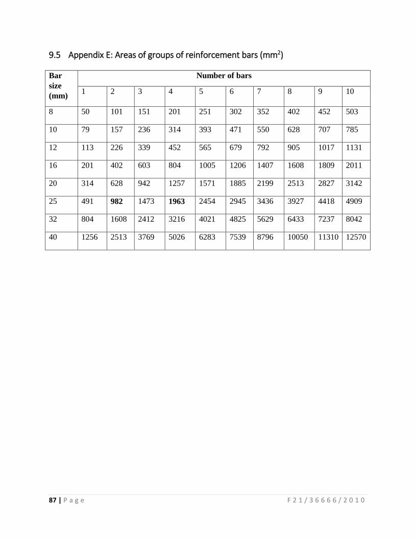
87 | P a g e F 2 1 / 3 6 6 6 6 / 2 0 1 0

9.5 Appendix E: Areas of groups of reinforcement bars (mm2)

Bar

size

(mm)

Number of bars

1 2 3 4 5 6 7 8 9 10

8 50 101 151 201 251 302 352 402 452 503

10 79 157 236 314 393 471 550 628 707 785

12 113 226 339 452 565 679 792 905 1017 1131

16 201 402 603 804 1005 1206 1407 1608 1809 2011

20 314 628 942 1257 1571 1885 2199 2513 2827 3142

25 491 982 1473 1963 2454 2945 3436 3927 4418 4909

32 804 1608 2412 3216 4021 4825 5629 6433 7237 8042

40 1256 2513 3769 5026 6283 7539 8796 10050 11310 12570

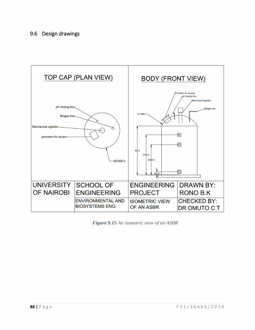
88 | P a g e F 2 1 / 3 6 6 6 6 / 2 0 1 0

9.6 Design drawings

Figure 9.15 An isometric view of an ASBR

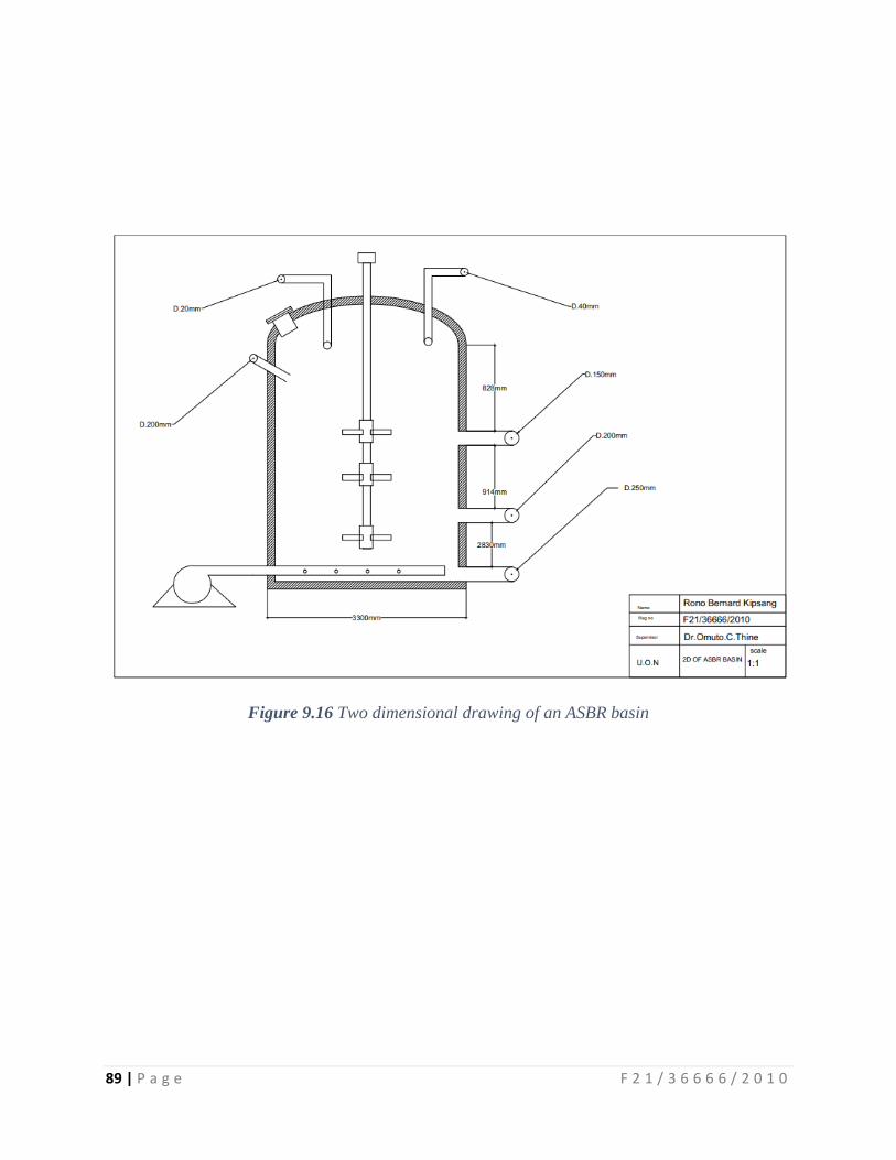
89 | P a g e F 2 1 / 3 6 6 6 6 / 2 0 1 0

Figure 9.16 Two dimensional drawing of an ASBR basin

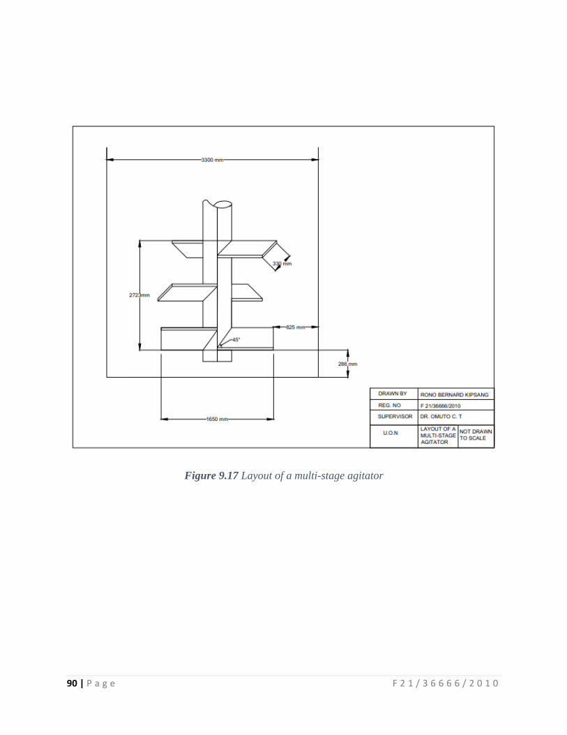
90 | P a g e F 2 1 / 3 6 6 6 6 / 2 0 1 0

Figure 9.17 Layout of a multi-stage agitator

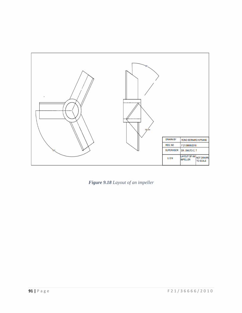
91 | P a g e F 2 1 / 3 6 6 6 6 / 2 0 1 0

Figure 9.18 Layout of an impeller

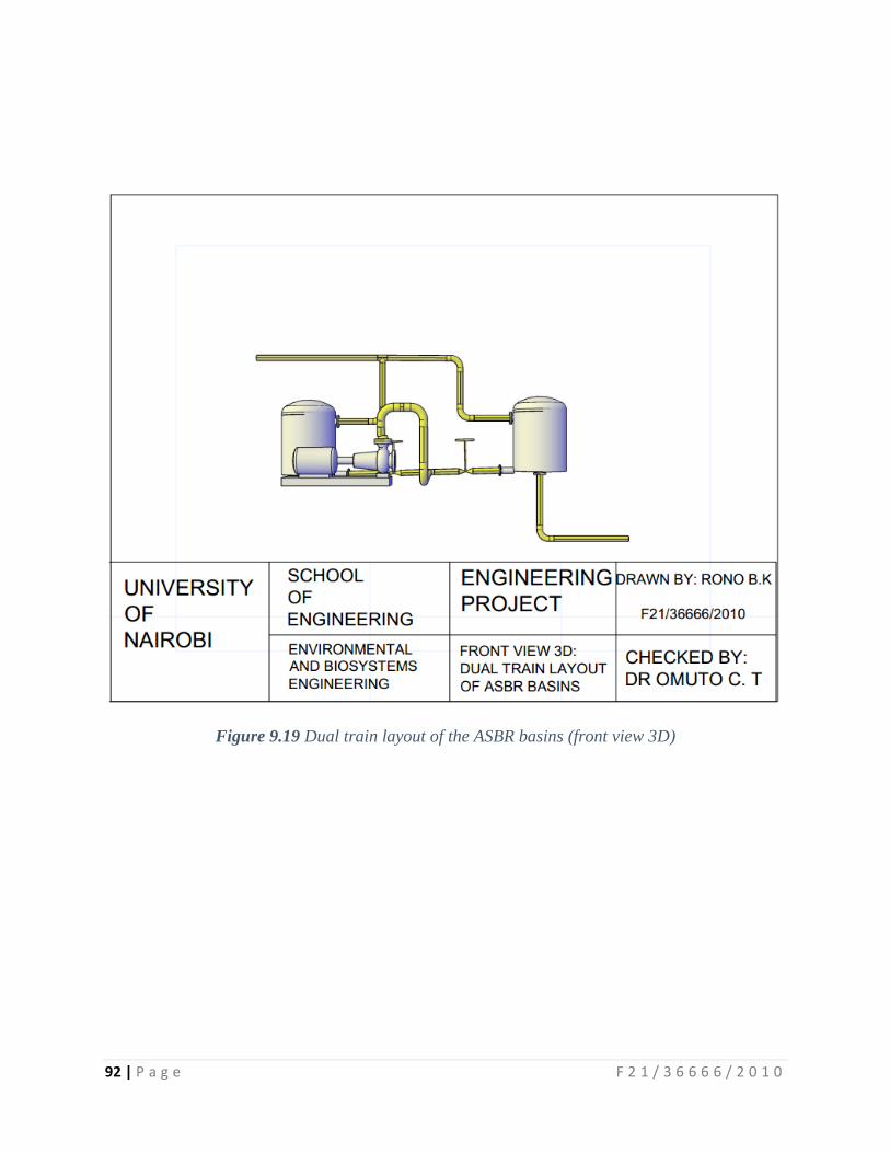
92 | P a g e F 2 1 / 3 6 6 6 6 / 2 0 1 0

Figure 9.19 Dual train layout of the ASBR basins (front view 3D)

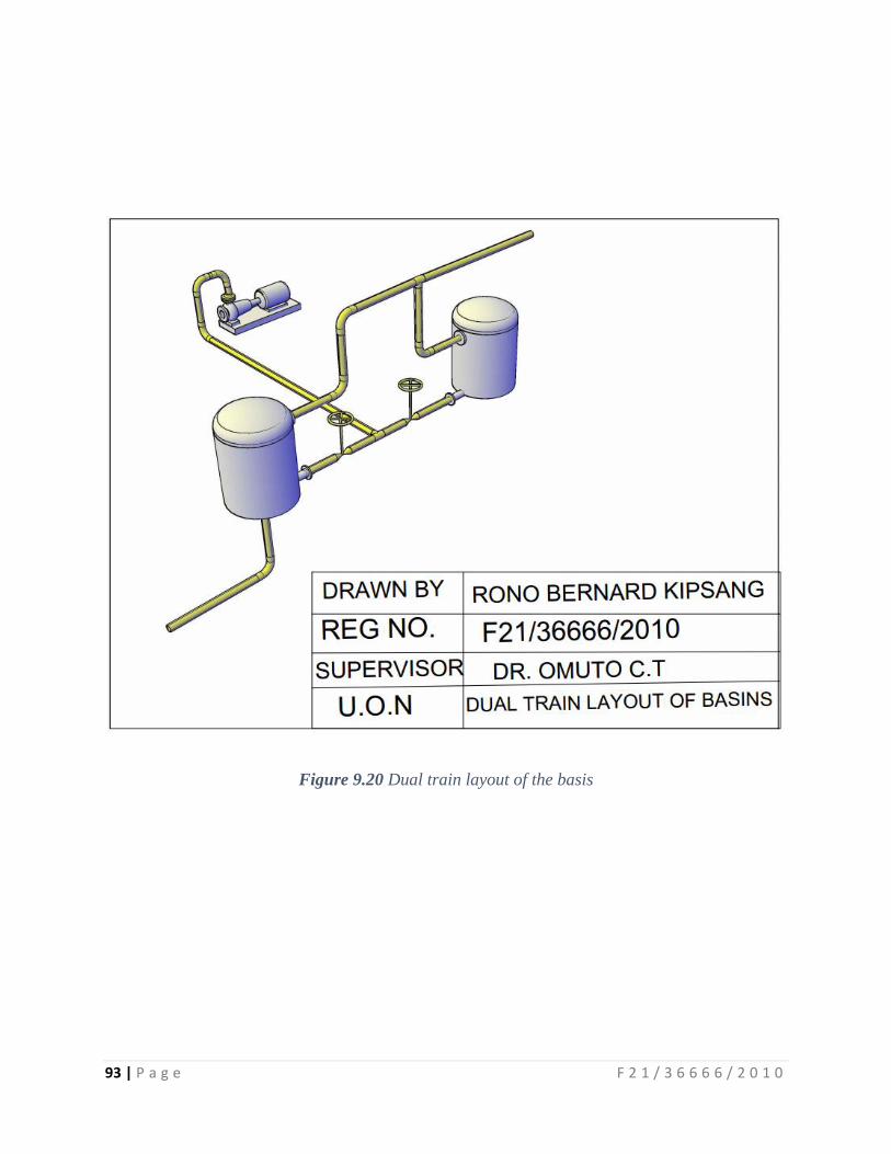
93 | P a g e F 2 1 / 3 6 6 6 6 / 2 0 1 0

Figure 9.20 Dual train layout of the basis