Embed Size (px)
Citation preview
UNIVERSITY OF OKLAHOMA
GRADUATE COLLEGE
SEISMIC ATTRIBUTE OPTIMIZATION WITH UNSUPERVISED MACHINE LEARNING
TECHNIQUES FOR DEEPWATER SEISMIC FACIES INTERPRETATION: USERS VS
MACHINES
A THESIS
SUBMITTED TO THE GRADUATE FACULTY
in partial fulfillment of the requirements for the
Degree of
MASTER OF SCIENCE
By
KARELIA LA MARCA
Norman, Oklahoma
2020
SEISMIC ATTRIBUTE OPTIMIZATION WITH UNSUPERVISED MACHINE LEARNING
TECHNIQUES FOR DEEPWATER SEISMIC FACIES INTERPRETATION: USERS VS
MACHINES
A THESIS APPROVED FOR THE
SCHOOL OF GEOSCIENCES
BY THE COMMITTEE CONSISTING OF
Dr. Heather Bedle. Chair
Dr. Brett Carpenter
Dr. Bradley Wallet

© Copyright by KARELIA LA MARCA 2020
All Rights Reserved.

iv
To Cloris and Roger: a couple of stars that guide my steps from the sky

v
ACKNOWLEDGEMENTS
Today I accomplished a beautiful episode where I gained knowledge and experiences I
never imagined before. The last two years shaped my character and set the foundations for my
future endeavors. Of course, that defending online and graduating in times of a pandemic was not
on the list! But for sure will be part of the memories that I will share with my children in the future.
Completing my M.Sc. thesis in these times has made me realize that, without essential people, this
achievement would not have been possible. Therefore, I want to express them my sincere gratitude:
The list starts with my advisors and confidants during the past two years: firstly, Dr. Slatt,
the person who changed my life by bringing me here to OU. He trusted me and showed me his
kind heart and infinite knowledge. He taught me to fall in love with the turbidites. He became my
role-model and, ultimately, my family. I hope I can make you feel proud and that you keep guiding
my steps from the skies. I was so lucky to have had you in my life! #slattgrad
I do have some angels above, but I also have one here on earth. Dr. Bedle appeared,
believed in me, and showed me how great seismic interpretation is. I feel so blessed because one
rarely finds an advisor that becomes your inspiration and friend. I cannot thank you enough for
everything you have done for me, and I cannot wait to start my Ph.D. with you and all the
adventures that are about to come :). Thank you for all the positiveness you bring even in the
hardest times.
I want to express my gratitude to my committee members: Dr. Carpenter, Dr. Brad Wallet.
Thank you for your advice and guidance. I also want to thank Dr. Marfurt for being inspirational
to me. I feel so lucky to have learned from top-notch professors. Therefore, I also want to thank
Dr. Pranter, Dr. Elmore, Dr. Mitra, Dr. Reza, and Jessica Reynolds for educating me, advising me,
and providing me with the strength to go through different situations.

vi
I am deeply thankful to my best friend and life companion, Javier Tellez. You have been
my strongest support in this journey. You taught me how we can turn an adverse situation in a
positive outcome when we are brave and perseverant enough. Thank you for your patience and
unconditional love.
I want to thank my family, especially my mom Zuleima, my sister Andrea and dad, Wime,
and Enrique. You are my main motivation. Everything I am today is because of you. I will always
be the little girl of yours, hoping to be as great and warmhearted as you all are.
To my Venezuelan childhood friends, principally, Estefania, Albany, Nohe, Ima, Yolmir,
Jose, Dayis, Grecia, Vane, Edwin, Marian, Shere, Oliver, Ana Martins and my PTS and WP teams.
Thanks for hearing me and supporting me whenever, despite the long distance. In the last years,
the University of Oklahoma became my home. OU added to my life unconditional friends like
Rafael Pires, Any Bustamante, Yuliana Zapata, Ariana Paez, Julian Chenin, Laura Ortiz, David
Lubo, Antonio Cervantes, Karen Leopoldinho, and Delcio Teixeira that supported me and truly
cared about me. I also collected unforgettable memories with Hannah, Hope, Fola, David Duarte,
Clayton Silver, Luis Castillo and Chris Ramos (the list goes long, but you know who you are).
Thank you to the SDA, AASPI, and IRC group for the regenerative feedback during my masters.
I also want to thank COLSA, AFV and its people to make me feel like home.
I express my gratitude to my Tapstone family, especially Adam Toy, Patrick McBride,
Nathan Acker, and Bryan Bottoms with whom I spent lovely times during last summer’ internship.
Last but not least, thank you to our main office girls, Ashley, Ginger, and Leah. Especial
thanks go to Rebecca Fay, who has helped me in uncountable ways! You are my life-saver.
Thank you all, and I hope the machines do not replace us, and we can see each other again soon
beyond our computer’s screens. Carpe Diem
vii
TABLE OF CONTENTS
ACKNOWLEDGEMENTS ........................................................................................................... V
LIST OF FIGURES ....................................................................................................................... X
LIST OF TABLES ..................................................................................................................... XVI
ABSTRACT .............................................................................................................................. XVII
CHAPTER I: INTRODUCTION .................................................................................................... 1
REFERENCES ............................................................................................................................ 2
CHAPTER 2: SEISMIC ATTRIBUTE SELECTION FOR UNSUPERVISED MACHINE
LEARNING TECHNIQUES FOR DEEPWATER SEISMIC FACIES INTERPRETATION ..... 3
ABSTRACT ................................................................................................................................ 3
INTRODUCTION ....................................................................................................................... 4
MOTIVATION AND OBJECTIVES ......................................................................................... 8
GEOLOGIC SETTING ............................................................................................................... 9
Miocene deepwater systems .................................................................................................... 9
SEISMIC DATASET AND DATA ........................................................................................... 11
Seismic data ........................................................................................................................... 11
Well data and other resources ............................................................................................... 11
THEORETICAL FUNDAMENTALS ...................................................................................... 12
Seismic attributes................................................................................................................... 12
SOMs: an unsupervised technique for seismic facies identification ..................................... 12
METHODS................................................................................................................................ 14
3D volume inspection and AOI definition ............................................................................. 14
Well tie ................................................................................................................................... 15
viii
Horizon picking/mapping ...................................................................................................... 15
Multi-attribute analysis and attribute selection for SOM ..................................................... 16
SOMs and interpretation ....................................................................................................... 18
RESULTS.................................................................................................................................. 19
Seismic expression of the AOI ............................................................................................... 19
Seismic attributes: finding the most suitable combination .................................................... 19
Testing non-linear relationships between attributes ............................................................. 21
SOMs - Interpretations per workflow .................................................................................... 22
Testing results, time evolution, and architectural elements .................................................. 24
DISCUSSION ........................................................................................................................... 25
CONCLUSIONS ....................................................................................................................... 29
ACKNOWLEDGMENTS ......................................................................................................... 30
FIGURES .................................................................................................................................. 31
TABLES .................................................................................................................................... 45
REFERENCES .......................................................................................................................... 48
APPENDIX ............................................................................................................................... 54
CHAPTER 3. USER VS MACHINE SEISMIC ATTRIBUTE SELECTION FOR
UNSUPERVISED MACHINE LEARNING TECHNIQUES: DOES HUMAN INSIGHT
PROVIDE BETTER RESULTS THAN STATISTICALLY CHOSEN ATTRIBUTES? ........... 55
INTRODUCTION ..................................................................................................................... 55
MOTIVATION ......................................................................................................................... 56
PRINCIPAL COMPONENT ANALYSIS (PCA) ..................................................................... 57
METHODOLOGY .................................................................................................................... 58
ix
RESULTS.................................................................................................................................. 59
Principal component analysis ............................................................................................... 59
Self-organizing maps analysis ............................................................................................... 60
SOMs results from user selected attributes vs machine derived inputs ................................ 61
Human vs machine comparison (upsides and downsides of PCA vs multi attribute analysis)
............................................................................................................................................... 62
CONCLUSION ......................................................................................................................... 64
ACKNOWLEDGMENTS ......................................................................................................... 65
FIGURES .................................................................................................................................. 66
TABLES .................................................................................................................................... 73
REFERENCES .......................................................................................................................... 74
x
LIST OF FIGURES
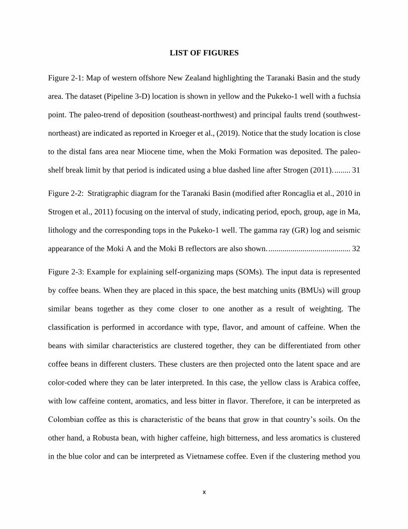
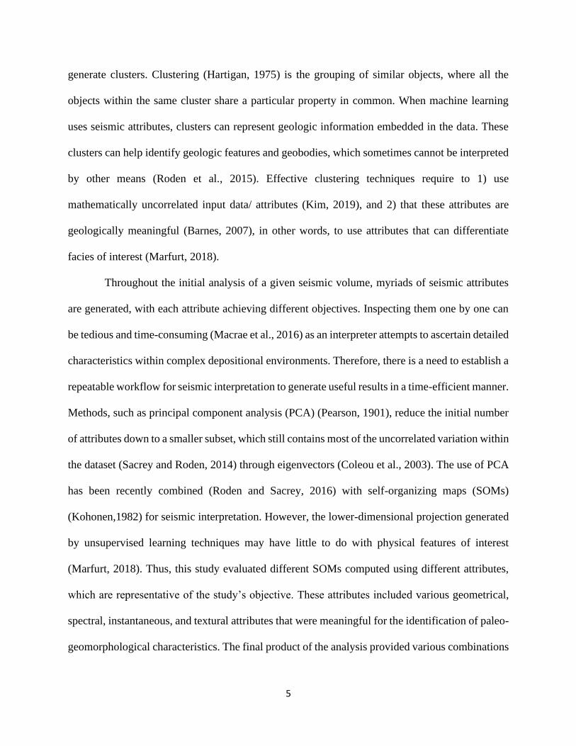
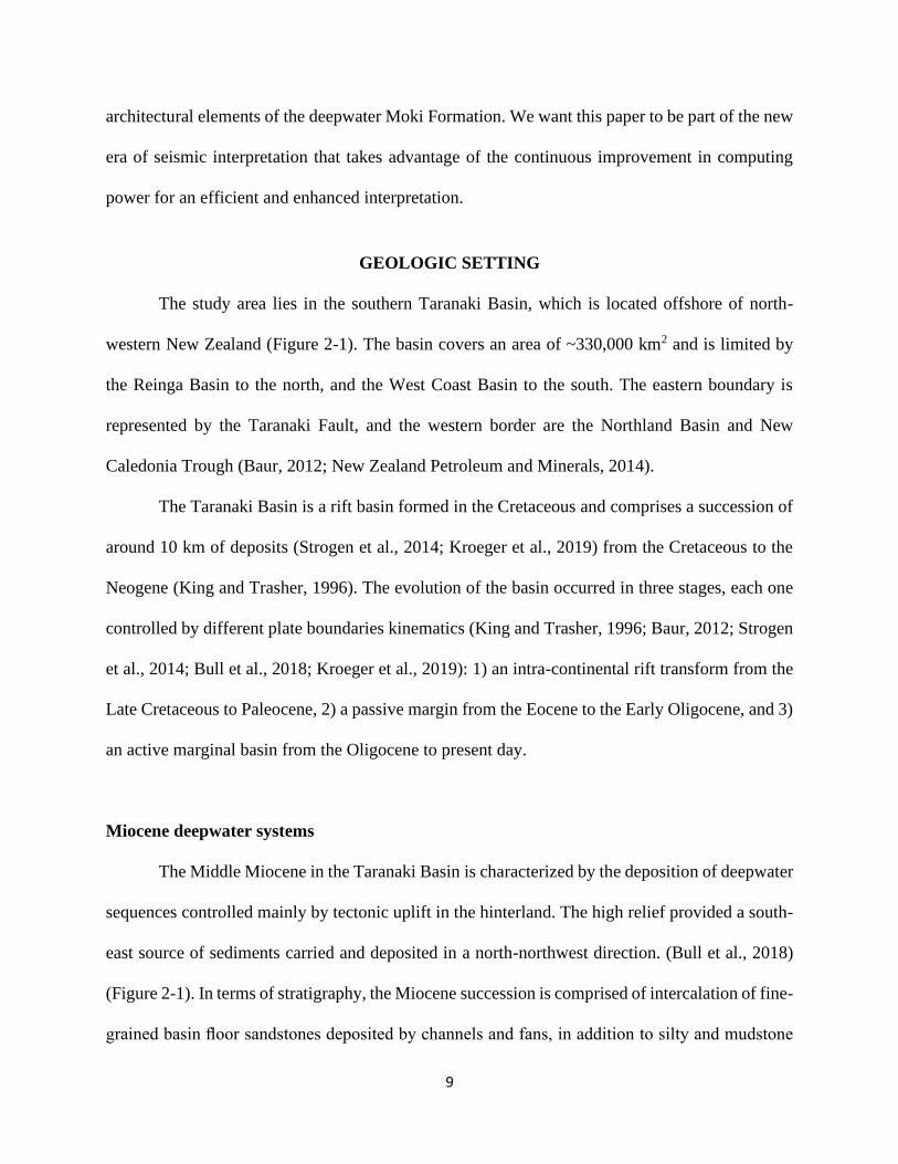
Figure 2-1: Map of western offshore New Zealand highlighting the Taranaki Basin and the study
area. The dataset (Pipeline 3-D) location is shown in yellow and the Pukeko-1 well with a fuchsia
point. The paleo-trend of deposition (southeast-northwest) and principal faults trend (southwest-
northeast) are indicated as reported in Kroeger et al., (2019). Notice that the study location is close
to the distal fans area near Miocene time, when the Moki Formation was deposited. The paleo-
shelf break limit by that period is indicated using a blue dashed line after Strogen (2011). ........ 31
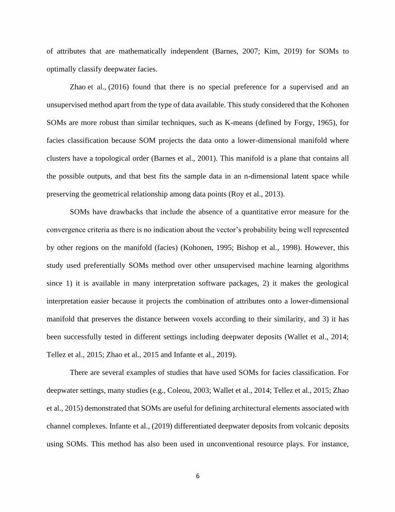
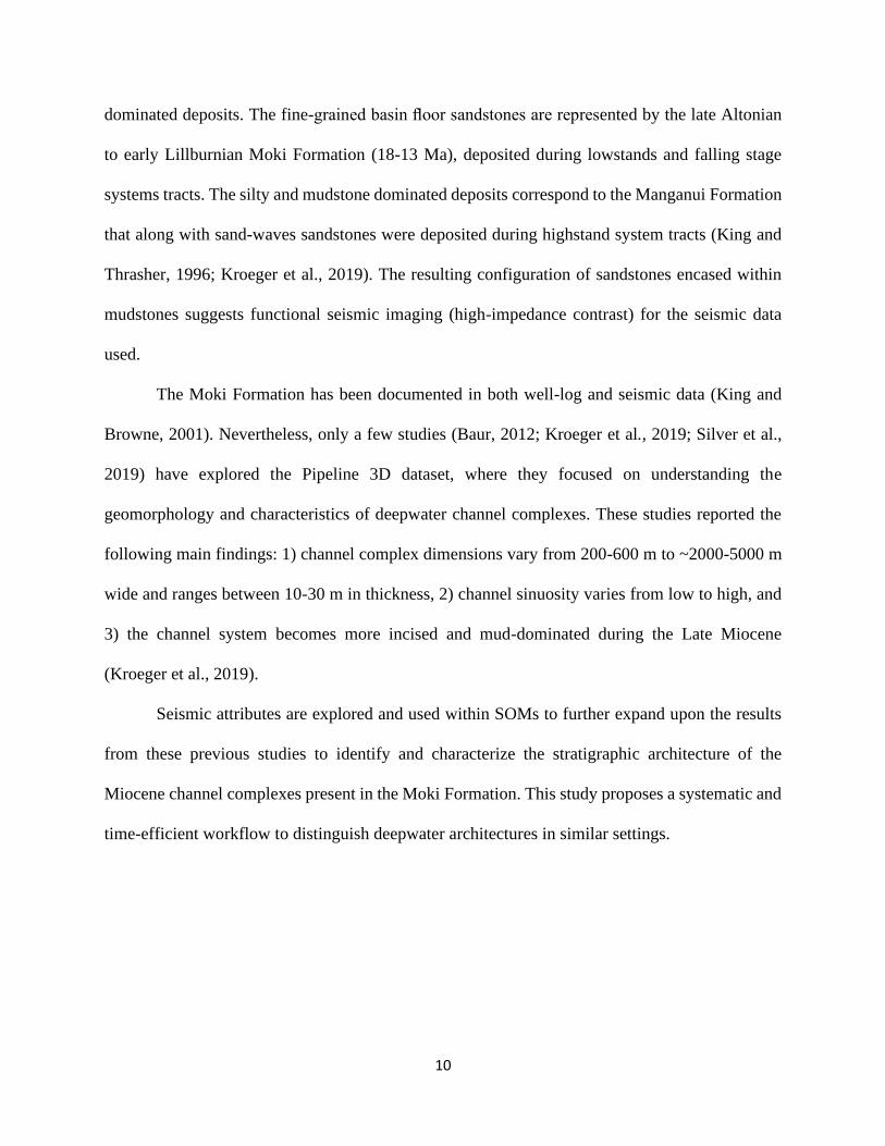
Figure 2-2: Stratigraphic diagram for the Taranaki Basin (modified after Roncaglia et al., 2010 in
Strogen et al., 2011) focusing on the interval of study, indicating period, epoch, group, age in Ma,
lithology and the corresponding tops in the Pukeko-1 well. The gamma ray (GR) log and seismic
appearance of the Moki A and the Moki B reflectors are also shown. ......................................... 32
Figure 2-3: Example for explaining self-organizing maps (SOMs). The input data is represented
by coffee beans. When they are placed in this space, the best matching units (BMUs) will group
similar beans together as they come closer to one another as a result of weighting. The
classification is performed in accordance with type, flavor, and amount of caffeine. When the
beans with similar characteristics are clustered together, they can be differentiated from other
coffee beans in different clusters. These clusters are then projected onto the latent space and are
color-coded where they can be later interpreted. In this case, the yellow class is Arabica coffee,
with low caffeine content, aromatics, and less bitter in flavor. Therefore, it can be interpreted as
Colombian coffee as this is characteristic of the beans that grow in that country’s soils. On the
other hand, a Robusta bean, with higher caffeine, high bitterness, and less aromatics is clustered
in the blue color and can be interpreted as Vietnamese coffee. Even if the clustering method you
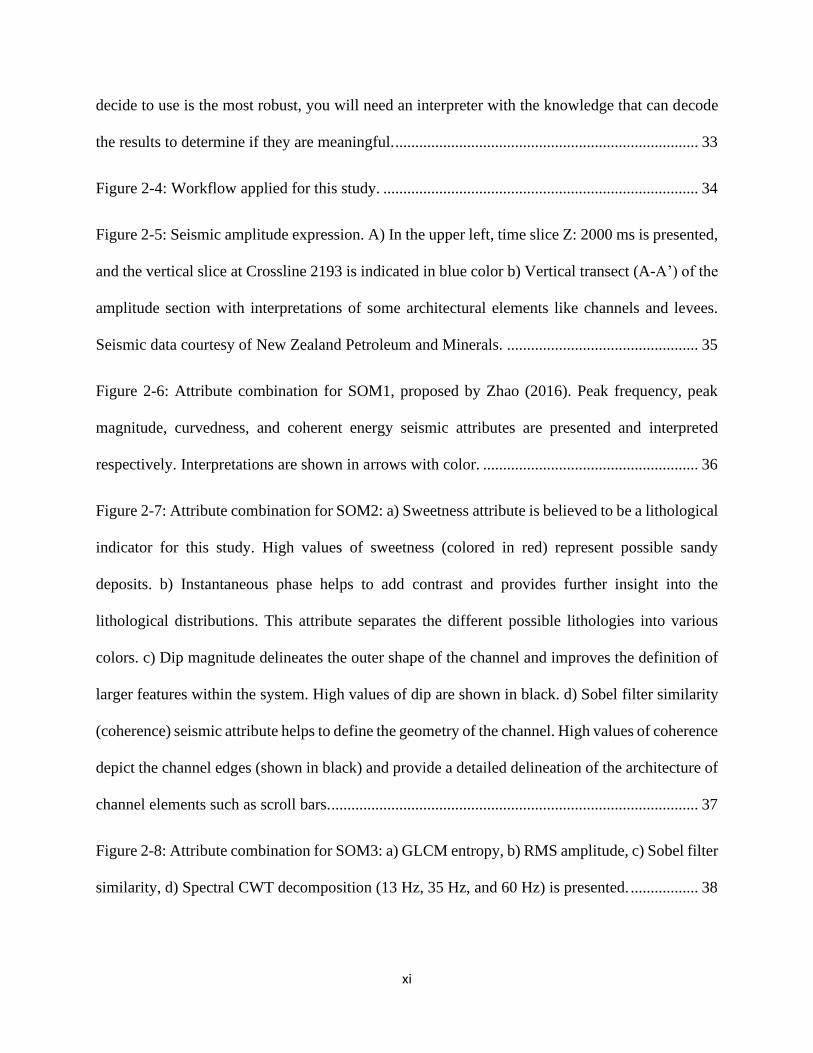
xi
decide to use is the most robust, you will need an interpreter with the knowledge that can decode
the results to determine if they are meaningful. ............................................................................ 33
Figure 2-4: Workflow applied for this study. ............................................................................... 34
Figure 2-5: Seismic amplitude expression. A) In the upper left, time slice Z: 2000 ms is presented,
and the vertical slice at Crossline 2193 is indicated in blue color b) Vertical transect (A-A’) of the
amplitude section with interpretations of some architectural elements like channels and levees.
Seismic data courtesy of New Zealand Petroleum and Minerals. ................................................ 35
Figure 2-6: Attribute combination for SOM1, proposed by Zhao (2016). Peak frequency, peak
magnitude, curvedness, and coherent energy seismic attributes are presented and interpreted
respectively. Interpretations are shown in arrows with color. ...................................................... 36
Figure 2-7: Attribute combination for SOM2: a) Sweetness attribute is believed to be a lithological
indicator for this study. High values of sweetness (colored in red) represent possible sandy
deposits. b) Instantaneous phase helps to add contrast and provides further insight into the
lithological distributions. This attribute separates the different possible lithologies into various
colors. c) Dip magnitude delineates the outer shape of the channel and improves the definition of
larger features within the system. High values of dip are shown in black. d) Sobel filter similarity
(coherence) seismic attribute helps to define the geometry of the channel. High values of coherence
depict the channel edges (shown in black) and provide a detailed delineation of the architecture of
channel elements such as scroll bars. ............................................................................................ 37
Figure 2-8: Attribute combination for SOM3: a) GLCM entropy, b) RMS amplitude, c) Sobel filter
similarity, d) Spectral CWT decomposition (13 Hz, 35 Hz, and 60 Hz) is presented. ................. 38
xii
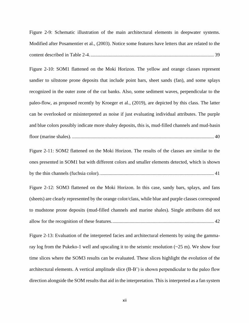
Figure 2-9: Schematic illustration of the main architectural elements in deepwater systems.
Modified after Posamentier et al., (2003). Notice some features have letters that are related to the
content described in Table 2-4. ..................................................................................................... 39
Figure 2-10: SOM1 flattened on the Moki Horizon. The yellow and orange classes represent
sandier to siltstone prone deposits that include point bars, sheet sands (fan), and some splays
recognized in the outer zone of the cut banks. Also, some sediment waves, perpendicular to the
paleo-flow, as proposed recently by Kroeger et al., (2019), are depicted by this class. The latter
can be overlooked or misinterpreted as noise if just evaluating individual attributes. The purple
and blue colors possibly indicate more shaley deposits, this is, mud-filled channels and mud-basin
floor (marine shales). .................................................................................................................... 40
Figure 2-11: SOM2 flattened on the Moki Horizon. The results of the classes are similar to the
ones presented in SOM1 but with different colors and smaller elements detected, which is shown
by the thin channels (fuchsia color). ............................................................................................. 41
Figure 2-12: SOM3 flattened on the Moki Horizon. In this case, sandy bars, splays, and fans
(sheets) are clearly represented by the orange color/class, while blue and purple classes correspond
to mudstone prone deposits (mud-filled channels and marine shales). Single attributes did not
allow for the recognition of these features. ................................................................................... 42
Figure 2-13: Evaluation of the interpreted facies and architectural elements by using the gamma-
ray log from the Pukeko-1 well and upscaling it to the seismic resolution (~25 m). We show four
time slices where the SOM3 results can be evaluated. These slices highlight the evolution of the
architectural elements. A vertical amplitude slice (B-B’) is shown perpendicular to the paleo flow
direction alongside the SOM results that aid in the interpretation. This is interpreted as a fan system
xiii
that was carved or incised by younger channels, and the system turns more mud prone as it
becomes younger (upwards). ........................................................................................................ 43
Figure 2-14: a) Crossline 2239 in seismic amplitude within the interval of study. b) Results of
SOM1 c) Results of SOM2, d) Results of SOM3. Notice how each SOM represents similar seismic
facies in different colors, and SOM3 appears to provide a more detailed classification. The
upscaled Pukeko-1 GR log is shown in the section. ..................................................................... 44
Figure 2-15: SOM3 results presented in a chair display. Sandy bars, splays, and fans (sheets) are
clearly represented by the orange color/class, while blue and purple classes correspond to silty to
mudstone prone deposits (marine shales in this case). Some levees are recognized in dark purple,
and overbank deposits in green. .................................................................................................... 45
Figure 3-1: Questions proposed for the study. .............................................................................. 66
Figure 3-2: Explanation of the main principal components derived from PCA. .......................... 66
Figure 3-3: Workflow for machine assisted attribute selection and comparison of methods in
Chapters 2 and 3............................................................................................................................ 67
Figure 3-4: Inline 1365 shown in amplitude. We selected a representative inline over which we
interpreted the PCA results. Some deepwater architectural elements are recognizable: channel
complex, levees, hemipelagic deposits, MTD and channelized lobes. Therefore, the attributes
contributing in each eigenvector should be related to these geological features. ......................... 68
Figure 3-5: Principal component analysis (PCA) results from 28 attributes shown in Table 3-1.
The first three eigenvectors (also known as principal components) represent the most of the
variation in the data. a) Eigenspectrum represented by a bar chart where each bar represents the
highest eigenvalue for each inline in the seismic 3D volume. Notice we selected a representative
xiv
inline (1965) for the analysis presented in b, c, and d. b) Principal component one (PC1)
represented with a yellow bar. The seismic attribute contribution is presented to the right. We
followed Leal et al., (2019) data analysis to select the most representative attributes. Therefore,
the selected attributes were those whose maximum percentage contribution to the principle
component was greater than or equal to 80%. In this case, GLCM, envelope and sweetness
attributes account for around 60% of the total variability in the data. c) Principal component two
(PC2) in yellow bar, to the right we find the main seismic attribute contributors. d) Principal
component three (PC3), represented by a yellow bar in the left, and the attribute selection based
on statistical contribution to the right. Depending on the interpretation objective, the highest
contributors (attributes) in each PC are possible candidates as input to a SOM or other
unsupervised ML technique. ......................................................................................................... 69
Figure 3-6: Self-organizing maps and inspection of individual neurons to determine which are
geologically meaningful and which represent random noise. ....................................................... 70
Figure 3-7: Self-organizing maps results from PCA is presented here, after filtering neurons
considered as noise or not geologically meaningful. Notice that out of the 16 neurons, we selected
6 that represent possibly architectural elements in the deepwater system evaluated. Neurons 1 and
8 represent bars, 1, more shaly and 8 sand rich. Neuron 2 denotes the shaley or hemipelagic
background and 4 the sheet sands that are fan like. Neurons 12 and 14 represent minor sized
features like overbanks and levees without much distinction between them. Similar clusters are
located close in the topological map. ............................................................................................ 71
Figure 3-8: Comparison between a) SOM derived from the PCA-selected attributes and b) the
SOM from the user selected attributes (Chapter 2). c) Amplitude has been provided to compare
where high amplitude areas may correspond to sandstone prone facies such as scroll bars and fans

xv
(sheet sands), but also to highlight the importance of the SOMs, since the architectural elements
are not distinguishable just in amplitude expression. The position of the Inline 1365 in Figure 2-4,
and Crossline 2239 shown below the time slices, are presented as reference. ............................. 72
xvi
LIST OF TABLES
Table 2-1: Common attributes, category, type, and interpretative use in geology (Modified from
Roden et al., 2015). ....................................................................................................................... 45
Table 2-2: List of attributes selected for deepwater seismic characterization in this study. The type
of attribute is indicated and explained according to the listed references (fourth column). The last
column describes the application of these attributes for seismic interpretation. .......................... 46
Table 2-3: List of the input attributes for each SOM. ................................................................... 46
Table 2-4: Architectural elements in deepwater settings. Schemes from Slatt and Weimer (2004)
are shown in each case. The seismic amplitude response and meaningful attributes for these
deepwater architectural elements are listed here. This table is inspired by Marfurt (2018). ...... 478
Table 2-5: Correlation matrixes from SOM1, SOM2, and SOM3. Main diagonals indicate the value
of 1 because it compares each attribute with itself. When comparing every other attribute, the
correlation is less than R = 0.7, which, according to Kim et al., (2019), represents the non-linear
relationship between the attributes. From this, every attribute used as an input for each SOM is
unique and representative of the dataset. ...................................................................................... 48
Table 3-1: List of input seismic attributes to PCA. Notice that a total of 28 attributes from different
types were considered to determine the main contributors in the section of interest. .................. 73
Table 3-2: List of input seismic attributes to PCA. Notice that a total of 28 attributes from different
types were considered to determine the main contributors in the section of interest. .................. 73
xvii
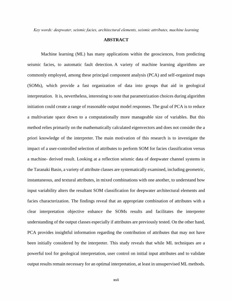
Key words: deepwater, seismic facies, architectural elements, seismic attributes, machine learning
ABSTRACT
Machine learning (ML) has many applications within the geosciences, from predicting
seismic facies, to automatic fault detection. A variety of machine learning algorithms are
commonly employed, among these principal component analysis (PCA) and self-organized maps
(SOMs), which provide a fast organization of data into groups that aid in geological
interpretation. It is, nevertheless, interesting to note that parametrization choices during algorithm
initiation could create a range of reasonable output model responses. The goal of PCA is to reduce
a multivariate space down to a computationally more manageable size of variables. But this
method relies primarily on the mathematically calculated eigenvectors and does not consider the a
priori knowledge of the interpreter. The main motivation of this research is to investigate the
impact of a user-controlled selection of attributes to perform SOM for facies classification versus
a machine- derived result. Looking at a reflection seismic data of deepwater channel systems in
the Taranaki Basin, a variety of attribute classes are systematically examined, including geometric,
instantaneous, and textural attributes, in mixed combinations with one another, to understand how
input variability alters the resultant SOM classification for deepwater architectural elements and
facies characterization. The findings reveal that an appropriate combination of attributes with a
clear interpretation objective enhance the SOMs results and facilitates the interpreter
understanding of the output classes especially if attributes are previously tested. On the other hand,
PCA provides insightful information regarding the contribution of attributes that may not have
been initially considered by the interpreter. This study reveals that while ML techniques are a
powerful tool for geological interpretation, user control on initial input attributes and to validate
output results remain necessary for an optimal interpretation, at least in unsupervised ML methods.
1
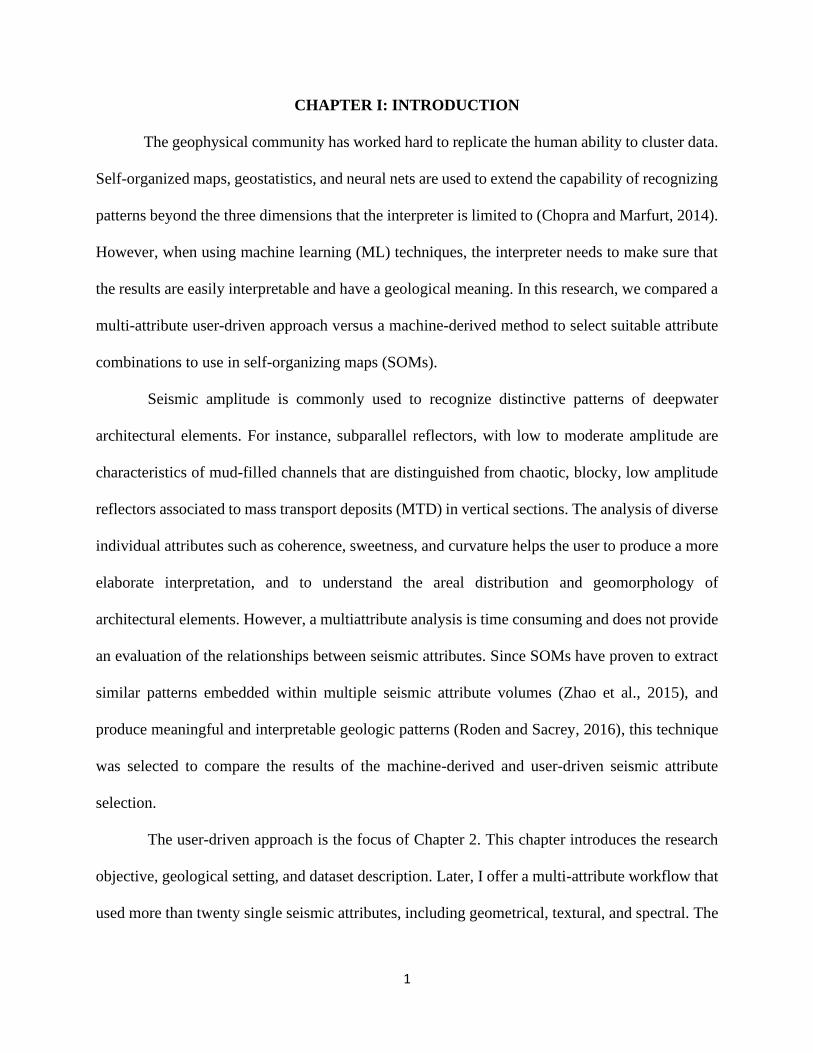
CHAPTER I: INTRODUCTION
The geophysical community has worked hard to replicate the human ability to cluster data.
Self-organized maps, geostatistics, and neural nets are used to extend the capability of recognizing
patterns beyond the three dimensions that the interpreter is limited to (Chopra and Marfurt, 2014).
However, when using machine learning (ML) techniques, the interpreter needs to make sure that
the results are easily interpretable and have a geological meaning. In this research, we compared a
multi-attribute user-driven approach versus a machine-derived method to select suitable attribute
combinations to use in self-organizing maps (SOMs).
Seismic amplitude is commonly used to recognize distinctive patterns of deepwater
architectural elements. For instance, subparallel reflectors, with low to moderate amplitude are
characteristics of mud-filled channels that are distinguished from chaotic, blocky, low amplitude
reflectors associated to mass transport deposits (MTD) in vertical sections. The analysis of diverse
individual attributes such as coherence, sweetness, and curvature helps the user to produce a more
elaborate interpretation, and to understand the areal distribution and geomorphology of
architectural elements. However, a multiattribute analysis is time consuming and does not provide
an evaluation of the relationships between seismic attributes. Since SOMs have proven to extract
similar patterns embedded within multiple seismic attribute volumes (Zhao et al., 2015), and
produce meaningful and interpretable geologic patterns (Roden and Sacrey, 2016), this technique
was selected to compare the results of the machine-derived and user-driven seismic attribute
selection.
The user-driven approach is the focus of Chapter 2. This chapter introduces the research
objective, geological setting, and dataset description. Later, I offer a multi-attribute workflow that
used more than twenty single seismic attributes, including geometrical, textural, and spectral. The
2
attribute user selection evaluated non-linear relationships between attributes to perform self-
organizing maps (SOMs) and characterize deepwater architectural elements in the Miocene Moki
Formation of the Taranaki Basin. I conclude with a recommended attribute combination to better
interpret and map the geological settings of the deepwater deposits based on geological criteria
with the obtained results.
The machine-driven approach, is presented in Chapter 3. I used Principal Component
Analysis (PCA) to reduce dimensionality and compare the user-driven insights obtained in Chapter
2 with the machine derived method. I explored and documented the advantages and disadvantages
of each method.
This research tests and evaluates the use of workflows to interpret deepwater settings. I
concluded that even though the use of machine learning methods is popular because of the increase
in computational power, these methods cannot fully replace interpreter’s prior knowledge. I show
how to take advantage of ML tools in a suitable manner to obtain efficient and valuable geological
results.
REFERENCES
Chopra, S; and K. J. Marfurt, 2014, Churning seismic attributes with principal component analysis:
86th annual international meeting, SEG, Expanded abstracts 2672-2676.
Roden, R., and Sacrey, D, 2016. Seismic interpretation with machine learning: GeoExpro. 13, 6.
pp 50-53 https://www.geoexpro.com/articles/2017/01/seismic-interpretation-with-
machine-learning
Zhao, T; V. Jayaram., A. Roy., and K. Marfurt, 2015, A comparison of classification techniques
for seismic facies recognition: Interpretation. 3, no. 4, SAE29-SAE58.
3
CHAPTER 2: SEISMIC ATTRIBUTE SELECTION FOR UNSUPERVISED MACHINE
LEARNING TECHNIQUES FOR DEEPWATER SEISMIC FACIES
INTERPRETATION
ABSTRACT
The task of finding the most direct and time-efficient methods for understanding the paleo-
geomorphological configuration of a hydrocarbon play to define the most prospective areas is
challenging, even for experienced seismic interpreters. Multi-attribute analysis provides
interpreters with valuable information that can accelerate paleo-geomorphological studies.
However, this approach requires a considerable amount of knowledge from the interpreter and
depending on the size of the 3D seismic volume, myriads of computing hours, which sometimes
could lead to meaningless results. The use of machine learning techniques, especially unsupervised
methods such as self-organizing maps (SOMs), has gained a significant foothold within the seismic
interpretation community to enhance results and to help identify similar patterns in the data. The
patterns identified from unsupervised learning possess geological meaning and can further aid in
the interpretation process if the input attributes are selected appropriately. We focused on the
inspection of a series of geometrical, instantaneous, spectral, and textural seismic attributes to
provide multi-attribute combinations that, along with SOMs, allows for a suitable interpretation of
architectural elements in deepwater settings. The results in the Miocene section (Moki Formation)
from the Pipeline 3D dataset, in the southern Taranaki Basin, show that the most important
considerations for attribute selection are that attributes 1) should be geologically meaningful, and
2) should be linearly independent. An appropriate combination of seismic attributes enhances the
SOMs results and further facilitates the interpretation of the features of interest. Results revealed
that, while machine learning techniques are a powerful tool for geological interpretation, the user’s
4
control on the initial input attributes and on the application of seismic geomorphology principles
for the resulting “in context” interpretation is still necessary for an optimal interpretation.
INTRODUCTION
The use of a single seismic attribute and combined seismic attributes have been common
practices for predicting rock properties for the past thirty years (Hart, 2011). Terms such as big
data and machine learning continue to gain popularity within the geoscience community. There
has been an increasing amount of interest in big data due to the vast amount of data available today.
Machine learning can be defined as various algorithms that automatically update themselves by
learning from the dataset. Machine learning techniques can predict rock properties or seismic
facies in a significantly smaller amount of time than an interpreter by finding relationships between
patterns which are not inherently obvious, and that can be often overlooked by an interpreter
(Sacrey and Roden, 2014; Zhao et al., 2016; La Marca-Molina et al., 2019). Therefore, we are at
the precipice of what Roden et al., (2015) consider “the next generation of advanced interpretation”
where experienced seismic interpreters can work in combination with advance machine learning
algorithms to better characterize and analyze the vast amount of geologic and geophysical data
present today (Zhao et al., 2016).
The majority of machine learning applications as they relate seismic volumes can be
expressed in terms of two categories: supervised and unsupervised learning. Pires de Lima (2019),
provides a brief review of different forms of supervised and unsupervised learning that can be
helpful for geoscientists. Our study used an unsupervised technique since no labels were applied,
and we wanted the algorithm to find natural patterns within the data, rather than to impose them.
This analysis used unsupervised machine learning to perform dimensionality reduction and to later
5
generate clusters. Clustering (Hartigan, 1975) is the grouping of similar objects, where all the
objects within the same cluster share a particular property in common. When machine learning
uses seismic attributes, clusters can represent geologic information embedded in the data. These
clusters can help identify geologic features and geobodies, which sometimes cannot be interpreted
by other means (Roden et al., 2015). Effective clustering techniques require to 1) use
mathematically uncorrelated input data/ attributes (Kim, 2019), and 2) that these attributes are
geologically meaningful (Barnes, 2007), in other words, to use attributes that can differentiate
facies of interest (Marfurt, 2018).
Throughout the initial analysis of a given seismic volume, myriads of seismic attributes
are generated, with each attribute achieving different objectives. Inspecting them one by one can
be tedious and time-consuming (Macrae et al., 2016) as an interpreter attempts to ascertain detailed
characteristics within complex depositional environments. Therefore, there is a need to establish a
repeatable workflow for seismic interpretation to generate useful results in a time-efficient manner.
Methods, such as principal component analysis (PCA) (Pearson, 1901), reduce the initial number
of attributes down to a smaller subset, which still contains most of the uncorrelated variation within
the dataset (Sacrey and Roden, 2014) through eigenvectors (Coleou et al., 2003). The use of PCA
has been recently combined (Roden and Sacrey, 2016) with self-organizing maps (SOMs)
(Kohonen,1982) for seismic interpretation. However, the lower-dimensional projection generated
by unsupervised learning techniques may have little to do with physical features of interest
(Marfurt, 2018). Thus, this study evaluated different SOMs computed using different attributes,
which are representative of the study’s objective. These attributes included various geometrical,
spectral, instantaneous, and textural attributes that were meaningful for the identification of paleo-
geomorphological characteristics. The final product of the analysis provided various combinations
6
of attributes that are mathematically independent (Barnes, 2007; Kim, 2019) for SOMs to
optimally classify deepwater facies.
Zhao et al., (2016) found that there is no special preference for a supervised and an
unsupervised method apart from the type of data available. This study considered that the Kohonen
SOMs are more robust than similar techniques, such as K-means (defined by Forgy, 1965), for
facies classification because SOM projects the data onto a lower-dimensional manifold where
clusters have a topological order (Barnes et al., 2001). This manifold is a plane that contains all
the possible outputs, and that best fits the sample data in an n-dimensional latent space while
preserving the geometrical relationship among data points (Roy et al., 2013).
SOMs have drawbacks that include the absence of a quantitative error measure for the
convergence criteria as there is no indication about the vector’s probability being well represented
by other regions on the manifold (facies) (Kohonen, 1995; Bishop et al., 1998). However, this
study used preferentially SOMs method over other unsupervised machine learning algorithms
since 1) it is available in many interpretation software packages, 2) it makes the geological
interpretation easier because it projects the combination of attributes onto a lower-dimensional
manifold that preserves the distance between voxels according to their similarity, and 3) it has
been successfully tested in different settings including deepwater deposits (Wallet et al., 2014;
Tellez et al., 2015; Zhao et al., 2015 and Infante et al., 2019).
There are several examples of studies that have used SOMs for facies classification. For
deepwater settings, many studies (e.g., Coleou, 2003; Wallet et al., 2014; Tellez et al., 2015; Zhao
et al., 2015) demonstrated that SOMs are useful for defining architectural elements associated with
channel complexes. Infante et al., (2019) differentiated deepwater deposits from volcanic deposits
using SOMs. This method has also been used in unconventional resource plays. For instance,
7
Verma et al., (2012), mapped high frackability and high TOC zones in the Barnett Shale, while
Sacrey and Roden (2014) located sweet spots in the Eagle Ford shale.
Our study focused on the definition of architectural elements on the Miocene deepwater
section of the Pipeline 3D, in the Taranaki Basin. The significance of differentiating good reservoir
architectural elements such as slope fans and scroll bars from that less reservoir-like such as levees
and shales resides in providing insights for exploration and production plans of an oil field. With
our study, we proposed a suitable multi-attribute approach that, with machine learning techniques,
allowed us to distinguish the architectural elements in the system better. The Taranaki Rift Basin
is the most prolific in terms of hydrocarbon production in New Zealand, and its tectonic and
stratigraphic evolution is well understood (King et al., 1996, 2000; Strogen et al., 2011, 2014;
Trasher et al., 2018). However, there are few studies that focused on the geomorphological
investigation of the architectural elements present within the Pipeline 3D dataset to evaluate the
distribution, size, and evolution of its channel complexes (Kroeger et al., 2019; Silver et al., 2019).
Additionally, there are no studies to this date that applied machine learning techniques to study
seismic facies or architectural elements in the Pipeline 3D dataset. Thus, our results are
contributing to previous studies developed in the Basin and pioneer in applying cutting edge
techniques for interpretation in the study area.
We built our method upon previous studies (e.g., Zhao et al., 2016; Infante et al., 2019) by
implementing a machine-learning interpretation workflow that involved the selection of relevant
and linear independent seismic attributes. These attributes were used as inputs for the SOMs to
identify deepwater architectural elements and are cross-correlated with well data (Pukeko-1) to
support the proposed interpretations.
8
The SOM models provided a list of attributes, their response, and their uses for
architectural elements recognition and interpretation to provide insights on the facies distribution
and temporal migration of channel complexes in the Miocene section. Additionally, the SOMs
here presented provided interpreters with a workflow that can be applied in similar settings to
efficiently characterize their features of interest.
MOTIVATION AND OBJECTIVES
The primary objective of this study was to inspect and find suitable combinations of
seismic attributes that are meaningful for geoscientists to use in SOMs to better characterize
architectural elements and seismic facies within a deepwater setting. This study allows
geoscientists to optimize the seismic attribute selection process resulting from post-stack time
migrated (PSTM) data and similar geological settings. This optimized selection process enables
the interpreter to create an efficient characterization of these features for an enhanced
interpretation. With the workflow proposed in this paper, architectural elements of deepwater
systems, such as mud and sand-filled channels, mass transport deposits (MTDs), and marine shales
in the basin floor, can be better mapped. Additionally, smaller features such as levees, overbank
deposits (splays), and sand waves can be further illustrated. The interpreter can select the best
reservoirs (usually bars/sand-filled channels, and sheet sands) from this architectural mapping, and
gain a better understanding of the channel’s migration over time, which can help optimize drilling
and production plans.
Furthermore, this paper represents the only study done so far on the Pipeline 3D dataset,
located in the Taranaki Basin, which applies an integrated workflow that carefully considers the
selection of attributes to be used in a SOM to better characterize the seismic facies and deepwater
9
architectural elements of the deepwater Moki Formation. We want this paper to be part of the new
era of seismic interpretation that takes advantage of the continuous improvement in computing
power for an efficient and enhanced interpretation.
GEOLOGIC SETTING
The study area lies in the southern Taranaki Basin, which is located offshore of north-
western New Zealand (Figure 2-1). The basin covers an area of ~330,000 km2 and is limited by
the Reinga Basin to the north, and the West Coast Basin to the south. The eastern boundary is
represented by the Taranaki Fault, and the western border are the Northland Basin and New
Caledonia Trough (Baur, 2012; New Zealand Petroleum and Minerals, 2014).
The Taranaki Basin is a rift basin formed in the Cretaceous and comprises a succession of
around 10 km of deposits (Strogen et al., 2014; Kroeger et al., 2019) from the Cretaceous to the
Neogene (King and Trasher, 1996). The evolution of the basin occurred in three stages, each one
controlled by different plate boundaries kinematics (King and Trasher, 1996; Baur, 2012; Strogen
et al., 2014; Bull et al., 2018; Kroeger et al., 2019): 1) an intra-continental rift transform from the
Late Cretaceous to Paleocene, 2) a passive margin from the Eocene to the Early Oligocene, and 3)
an active marginal basin from the Oligocene to present day.
Miocene deepwater systems
The Middle Miocene in the Taranaki Basin is characterized by the deposition of deepwater
sequences controlled mainly by tectonic uplift in the hinterland. The high relief provided a south-
east source of sediments carried and deposited in a north-northwest direction. (Bull et al., 2018)
(Figure 2-1). In terms of stratigraphy, the Miocene succession is comprised of intercalation of fine-
grained basin floor sandstones deposited by channels and fans, in addition to silty and mudstone
10
dominated deposits. The fine-grained basin floor sandstones are represented by the late Altonian
to early Lillburnian Moki Formation (18-13 Ma), deposited during lowstands and falling stage
systems tracts. The silty and mudstone dominated deposits correspond to the Manganui Formation
that along with sand-waves sandstones were deposited during highstand system tracts (King and
Thrasher, 1996; Kroeger et al., 2019). The resulting configuration of sandstones encased within
mudstones suggests functional seismic imaging (high-impedance contrast) for the seismic data
used.
The Moki Formation has been documented in both well-log and seismic data (King and
Browne, 2001). Nevertheless, only a few studies (Baur, 2012; Kroeger et al., 2019; Silver et al.,
2019) have explored the Pipeline 3D dataset, where they focused on understanding the
geomorphology and characteristics of deepwater channel complexes. These studies reported the
following main findings: 1) channel complex dimensions vary from 200-600 m to ~2000-5000 m
wide and ranges between 10-30 m in thickness, 2) channel sinuosity varies from low to high, and
3) the channel system becomes more incised and mud-dominated during the Late Miocene
(Kroeger et al., 2019).
Seismic attributes are explored and used within SOMs to further expand upon the results
from these previous studies to identify and characterize the stratigraphic architecture of the
Miocene channel complexes present in the Moki Formation. This study proposes a systematic and
time-efficient workflow to distinguish deepwater architectures in similar settings.
11
SEISMIC DATASET AND DATA
Seismic data
The 3D seismic dataset used for this study is named Pipeline 3D. This seismic survey was
acquired in 2013 by Todd Exploration and covered ~515 km2 of the southern Taranaki Basin
(Figure 2-1). The data is zero phase and has SEG negative polarity (a positive change in acoustic
impedance is represented by a trough). The survey has a ~25 m of vertical resolution, with a sample
interval of 4 ms, a bin size of 25 m by 12.5 m and a total record length of 6 s. The projection datum
is NZGD2000. The PSTM volume was processed by Excel Geophysical services in 2015. This
data was provided by New Zealand Petroleum and Minerals.
Well data and other resources
Within the Pipeline 3D, one well titled Pukeko-1 (Figure 2-1) was incorporated in our study
to test our results. The Pukeko-1 was drilled in 2004 and reached a total depth of 4190 m (New
Zealand Petroleum and Minerals, 2014). This well, whose main objective was the Eocene Kapuni
group, was abandoned due to no commercial hydrocarbon return. Our section of interest
corresponds to the Miocene Moki and Manganui Formations, located between ~2141 m and ~2800
m (Figure 2-2). A gamma-ray log (GR) is available for the section of interest. Other data includes
a report which has lithology descriptions that define a fine-grained Moki Formation interbedded
with siltstones and mudstones (Manganui Formation). A check-shot in the well establishes an
accurate time-depth relation with the seismic dataset. All well data was provided courtesy of the
New Zealand Petroleum and Minerals.
12
THEORETICAL FUNDAMENTALS
Seismic attributes
A seismic attribute is any measure of seismic data that helps us visually enhance or quantify
features of interest for interpretation (Chopra and Marfurt, 2007). Seismic attributes are a response
of the rocks’ physical properties. Therefore, the spatial distribution and relationships of these
responses, along with geological context, help to make reliable seismic interpretations. A single
attribute is not enough for extracting all the potential information present in the seismic data
(Chopra and Marfurt, 2014). Thus, we usually combine attributes in a multi-attribute analysis
(Taner and Sheriff, 1977; Russell and Hampson, 1997) or, such as the case in this study, are used
in SOMs to extract geological information all at once.
In Table 2-1, Roden and Sacrey (2015) present a list of common seismic attributes, their
type, and interpretive use. Geometric attributes such as dip, coherence, and curvature help in
delineating the geometry or shape of the channel, and attributes such as the instantaneous phase
and sweetness could be reliable lithological indicators (La Marca-Molina et al., 2019). Grey level
co-occurrence matrix (GLCM) texture attributes are useful for the determination of seismic facies
analysis (Chopra and Marfurt, 2014) as these attributes quantify the uniformity or disorder in the
image. Frequency attributes help to interpret bed thicknesses, discontinuities, and fluids (Partyka
et al., 1999). More information about attributes and their use in facies characterization is available
in Taner (1979), Barnes (2001), Liu (2007), Chopra and Marfurt (2007), and Marfurt (2018).
SOMs: an unsupervised technique for seismic facies identification
A SOM is an unsupervised (feed-backward) machine learning technique that was first
introduced by Kohonen in 1982 and is frequently used in many areas such as in technology (e.g.,
13
An and Yu, 2012), in marketing (e.g., Hanafizadeh and Mirzazadeh, 2010), in medicine (e.g.,
Tuckova et al., 2011) and in environmental applications (e.g., Gibson et al., 2017) to find patterns
with similar characteristics within their respective datasets. Roy et al., (2013) describe how this
machine learning method has been used since the late 1990s in the oil industry to resolve diverse
geoscience interpretation problems. For example, SOMs have been adapted to be used in seismic
facies identification as it extracts similar patterns embedded within multiple seismic attribute
volumes (Zhao et al., 2015). With modern visualization capabilities and the application of 2D color
maps (Gao, 2007), SOMs routinely produce meaningful and easily interpretable geologic patterns
(Roden and Sacrey, 2016).
Humans are good at pattern recognition, yet the task of finding the relationship between all
the data points at the same time is cumbersome, if not impossible. SOMs attempt to solve this issue
by reducing the number of dimensions and illustrating these similarities (Roden et al., 2015) onto
a 2D lower dimensional space where these output groups (e.g., clusters) are easier to interpret.
The SOM algorithm details are presented in Kohonen (1982). We use a coffee bean analogy
to explain how SOMs can classify these beans based off on their flavor, morphology, and amount
of caffeine (Figure 2-3). We can summarize the process in four steps:
1) Input data and initialization: coffee bean attributes that have a characteristic flavor,
morphology, and amount of caffeine, are used as the input.
2) Weighting and best matching unit (BMU) definition (sometimes referenced as the winning
neuron), where a neuron learns by adjusting its position within the attribute space as it is
drawn toward nearby data samples. Once the learning process has completed, the winning
neuron set is used to classify each selected multiattribute sample in the survey (Roden et al.,
2015).

14
3) Clustering: Given the BMU, each attribute sample in the dataset incrementally approaches
towards a similar BMU in each case by the Euclidean distance. A SOM manifold that
contains all the possible combinations is then formed, and the algorithm deforms this
manifold to better fit the data in each iteration (Zhao et al., 2016).
4) Projection of clusters in a lower 2D dimensional space where colors are assigned. Gao (2007)
mentions that if the number of prototype vectors is 256, we will have 256 colors. These are
the potential clusters. Our results can form either 256 or considerably a smaller number of
clusters (e.g., three or four). Finally, after clusters or classes are obtained, the interpreter uses
their knowledge to make geological interpretations of these clusters.
METHODS
The workflow applied in this study is presented in Figure 2-4. Important details of each
phase of the workflow are given as follows:
3D volume inspection and AOI definition
Preliminary inspection of the seismic volume is paramount for identifying acquisition
footprint, noise, and other features that can influence the interpretation. Also, this inspection helps
the interpreter identifying prominent features and the potential areas of interest (AOIs) within the
seismic volume. We use amplitude and coherence volumes to perform this preliminary analysis by
scanning through various, inlines, crosslines, and time slices.
Depending on the focus of the study and objective, the interpreter selects an AOI, and crops
the initial seismic volume to the AOI extent. In our case, we chose an AOI of ~300 km2 as it
comprises the channel complexes while also avoiding the structural influence of a large-scale fold
15
present in the area. This structural feature was omitted from the SOM as it can affect the
classification. Vertically, the AOI includes the Miocene Moki and Manganui Formations. These
deepwater formations are located at around 1800-2300 ms in two-way travel time within the
seismic record. We defined the AOI vertical window of 500 ms as it captures the same type of
deposits that should be genetically related (facies). Therefore, by using a small window, in addition
to a representative AOI, the algorithms can process information more efficiently and further avoid
miscalculations and misclassifications.
Well tie
The Pukeko-1 well contains check shot data and well tops (New Zealand Overseas
Petroleum Ltd., 2004), which facilitates a depth-time conversion and a well tie. This well tie allows
for the recognition of the geological formations and the lithological responses present within each
interval in the seismic. Although the 25 m seismic resolution of our volume is insufficient to
characterize the geological sequences in detail, well logs (as GR) are useful for identifying not
only lithology but to also further support the architectural elements due to the logs’ characteristic
signatures and trends.
Horizon picking/mapping
There are several visualization techniques to represent seismic attributes with the aim of
performing geological interpretation. Some of these are vertical and horizontal slices, horizon
slices, stratal slices, phantom horizon slices, box probes, etc. (e.g., Posamentier, 2015). The
visualization techniques used depend on the purpose of the study. In the case of this study, time
slices are not appropriate for analyzing the same architectural elements that share similar
16
depositional settings at the same geological time. Therefore, by picking horizons parallel to the
reflectors of the AOI, a better representation of the deepwater system can be created upon
extracting seismic attributes or flattening seismic attribute volumes onto these reflectors. We
fattened the seismic volumes on the Moki Horizon (Figure 2-5). This horizon was picked by
following a clear and continuous reflector (a peak). We interpreted the horizon every ten lines, in
an inline-crossline sequence, to better map the reflector. After completing the interpretation, we
used automatic tracking. We then evaluated the automatic tracking results in non-continuous
reflector zones, such as in channel valleys, where interpolation can sometimes underperform. We
corrected the horizon manually where necessary.
Multi-attribute analysis and attribute selection for SOM
How to select the right attributes?
Seismic interpretation begins by defining the objective of the study (Roden and Sacrey,
2016) and by performing a data quality check. It is paramount to have a clear goal while
interpreting so that the appropriate seismic attributes are selected to best suit the purpose of the
study and geological setting (Roy et al., 2003). This first phase allows for an optimal, preliminary
selection of attributes. For example, if the study is predominantly structural, then the use of
geometrical details may provide better results than using just spectral attributes. This study aimed
to identify different seismic facies and architectures that correspond to deepwater deposits found
within the Miocene Moki Formation. Therefore, attributes that could differentiate mud-filled
channels from sand-filled ones and isolate MTD, and overbank deposits were selected. There is a
myriad of attributes that can be tested, such as amplitude versus offset (AVO) attributes to optimize
classifications, mainly when the objective implies hydrocarbon detection. However, when the
17
dataset is a PSTM volume, the attributes that can be calculated are limited on this type of seismic
data and should be a crucial consideration for all interpreters.
We explored geometric, spectral, instantaneous, and texture attributes to find the most
suitable attributes to incorporate into the SOM models for deepwater seismic facies
characterization. We selected geometrical (discontinuity) attributes because they are commonly
used to define the outer shape or geomorphology of geological features (Chopra et al., 2007).
GLCM textural attributes aid in facies identification (Haralick et al., 1973). Spectral and
instantaneous attributes, on the other side, are known for unraveling lithological content (Marfurt,
2006), and their capability of distinguishing differently sized features associated with channel
complexes (Partyka et al., 1999): small architectures like levees are usually related to high
frequencies, and significant, master channels can be identified with small frequencies.
For attributes calculation, we used the AASPI (Attribute Assisted Seismic Processing and
Interpretation) software provided to the University of Oklahoma School of Geosciences.
Polychromatic color bars were used to better visualize the internal behavior (Barnes, 2001) related
to seismic properties, and monochromatic color bars were used to visualize the edges. Some of the
attributes were co-rendered to improve the interpretation, as suggested by Posamentier (2015). Co-
rendering allows the interpreter to concentrate on features of interest. The result section presents
the attributes selected for each workflow (SOMs). Attribute volumes were extracted and flattened
on the Moki Horizon to perform better interpretations of the architectural elements.
Before incorporating the various attributes into the SOM, they should be linearly
independent (Kim et al., 2019), to avoid using redundant attributes that are similar to each other.
We analyzed the co-variance matrices in each attribute combination to define the most suitable

18
ones. We selected attribute combinations were the linear relationship between each attribute with
the others resulted in R < 0.7, as suggested by Kim et al., (2019).
SOMs and interpretation
The SOM algorithm was selected over other similar unsupervised learning techniques for
the following reasons:
1) It allows for the integration of three or more attributes which can highlight features that are
not easily recognizable by a single attribute or through co-rendering;
2) It is a method that is relatively easy to apply;
3) It is available in at least three interpretation software packages.
Although SOMs appear to be advantageous over similar unsupervised learning methods,
there are some limitations. Kohonen (1995) and Bishop (1998) identified these caveats as follows:
1) The selection of the neighborhood option in each iteration is subjective so that different
solutions derive after each iteration;
2) There is an absence of a quantitative error to define the convergence acceptance;
3) SOMs do not provide a quantitative confidence measure in the facies classification.
This study’s proposed workflow can mitigate some of these uncertainties by having some
geological biases in the input data, which in this case, are the selected seismic attributes.
We used AASPI for calculating the SOMs and was parametrized by defining 256 clusters
(prototype vectors). The SOMs were then exported into a commercial interpretation package to
visualize and interpret the results, where each SOM was flattened on the Moki Horizon. Available
GR logs from the Pukeko-1 well were also incorporated into the SOM analysis and were upscaled
to the resolution of the seismic data (~25 m).
19
RESULTS
Seismic expression of the AOI
Before exploring the different seismic attributes, we evaluated the seismic amplitude
character in the AOI. Figure 2-5 shows an amplitude time slice at -2000 ms. In Crossline 2193 (A-
A’ in Figure 2-5), we observe the intersection of different size channels (100 m to 3000 m wide)
and their variable amplitudes. Some of these channels are incised, exhibiting basal scour surfaces,
and different infill patterns. These features are shown through the typically low amplitude and
stacked reflector responses. Overall, the reflector configurations range from more conformable in
deeper sections to more chaotic as it becomes shallower. A continuous, high amplitude reflector
(trough) above the Moki Horizon is associated with sheet sands due to its high amplitude response
and lateral continuity. We interpret some levees to be associated with the main channel belts. Table
2-4 explains the internal seismic reflection, external shape, and amplitude character of the
architectural elements recognized in the dataset. Notice that although amplitude is a good
preliminary tool to identify some architecture and facies, especially on vertical slices, it does not
define the dimensions or aerial extent of the architectural elements. Therefore, it is necessary to
integrate other attributes to create a more accurate characterization of these features.
Seismic attributes: finding the most suitable combination
Attributes that have geological significance for deepwater facies were chosen after
exploring various geometrical, textural, spectral, and instantaneous attributes. The chosen
attributes are those that can better highlight geomorphologic or stratigraphic features. Table 2-2
presents the list of attributes selected, indicating their types, explaining its principle, and
20
supporting references. The common geological interpretation of each attribute is shown in each
case.
Secondly, the list of attributes was reduced by ensuring that these attributes are linearly
independent (Barnes, 2007; Kim et al., 2019). Table 2-3 shows the combinations used for each
SOM model. The attribute combinations for SOM1 were identical to the attributes used by Zhao
(2016), who studied deepwater seismic facies in the Canterbury Basin. By selecting the same
attributes as Zhao (2016) for SOM1, we evaluated his approach in a different area, which still
shares a similar geological setting. The second seismic-multi-attribute workflow explores the
combination of geometrical attributes with attributes that are a useful indicator of lithology. The
third combination evaluates the contribution of textural and spectral attributes. Ultimately, we
aimed to test the different SOM responses by using various combinations of different attribute
types.
We evaluated the geologic response of the attributes when comparing among each other
after flattening on the Moki Horizon. Curvedness (Figure 2-6a), dip magnitude (Figure 2-7c), and
sobel filter similarity (Figure 2-7d) highlight the geomorphology of architectural elements within
the channel belt complexes such as channels, levees, scroll bars, splays, and abandoned channels.
Most positive curvature, K1, (Figure 2-7e) is particularly useful for defining the levees and smaller
channels associated with the master channel and to further differentiate various deepwater
architectural elements. Additionally, sweetness, root mean square (RMS), and instantaneous phase
are good lithological indicators (Figure 2-8b). High values of sweetness denote possible sandstone
rich areas (Figure 2-7a), such as sandy lobes (sheets), sandy bars, and some splays. These high
sweetness areas often coincide with high RMS values zones (Figure 2-8b).
21
Textural attributes belong to a different category of seismic attributes. In this study, GLCM
entropy emphasizes changes in textures, whose interpretation is associated with different facies
(Figure 2-8a). Therefore, this attribute is a useful input for the SOM algorithm as it will better
characterize different deepwater facies. Sand prone deposits exhibit low GLCM entropy values,
whereas more mud-prone and chaotic (such as MTDs) deposits are represented by higher GLCM
values.
Spectral decomposition is a widely used technique for channel studies (Partyka et al.,
1999). The incorporation of different frequency components with other input attributes into the
SOM model can help to further differentiate facies and architectures of different thicknesses (e.g.,
levees and channels). The Pipeline 3D dataset contains a frequency spectrum which varies from 5
Hz to almost 100 Hz. The dataset’s dominant and representative frequencies within the AOI of 13,
35, and 60 Hz, were RGB blended (Figure 2-8d). Smaller frequencies are useful for defining the
major architectural elements, like channels, whereas higher frequencies highlight minor features,
such as levees or splays (Figure 2-8d).
Figure 2-9 shows a schematic representation of the location of various deepwater elements
from proximal to distal areas. Table 2-4 presents the seismic expression of the various deepwater
architectural elements recognized in this study in addition to their responses within the meaningful
seismic attributes. Note that the elements in Table 2-4 appear in Figure 2-9 with letters to show
their relative position in the system.
Testing non-linear relationships between attributes
Kim (2019) states that while relevant attributes preserve a relationship with the output
classes, redundant attributes have a higher correlation between them. This is the reason for
evaluating the linear relationship between attributes to better optimize our SOM models.
22
Table 2-5 presents a correlation matrix for each SOM model. The main diagonal presents
values of one (1) since it is comparing the same seismic attribute with itself. For each attribute
combination explored, attributes that had a correlation smaller than 0.7 were considered as input
to be used in the various SOM models as this value indicated that there is a weak linear relationship
amongst the list of attributes selected.
SOMs - Interpretations per workflow
We evaluated the results of each of the SOM results by flattening their volumes on the
Moki Horizon so that features of interest are comparable between the different SOM models. We
applied principles of seismic geomorphology to interpret the different architectural elements
present within the AOI. The word “workflow” refers to the combination of attributes selected for
each SOM. The results of each workflow are presented as follows:
Workflow 1- (SOM1)
SOM1 uses a combination of attributes that are beneficial for deepwater facies
characterization after studies from Zhao et al., (2016). SOM1 was calculated by combining peak
frequency, peak magnitude, coherent energy, and curvedness seismic attributes (shown in Figure
2-10). The yellow and orange colors (or classes) represent more sand-prone deposits, which
include point bars and sheet sands (fan-lobe) as well as some sediment waves as defined recently
by Kroeger et al., (2019). These sediment waves are perpendicular to the paleo-flow direction,
which follows a southeast-northwest trend, and can be sometimes overlooked or misinterpreted as
noise when only looking at a single attribute. The purple and blue colors possibly indicate more
shaley elements such as mud-filled channels, and marine shales commonly found in the basin floor.
23
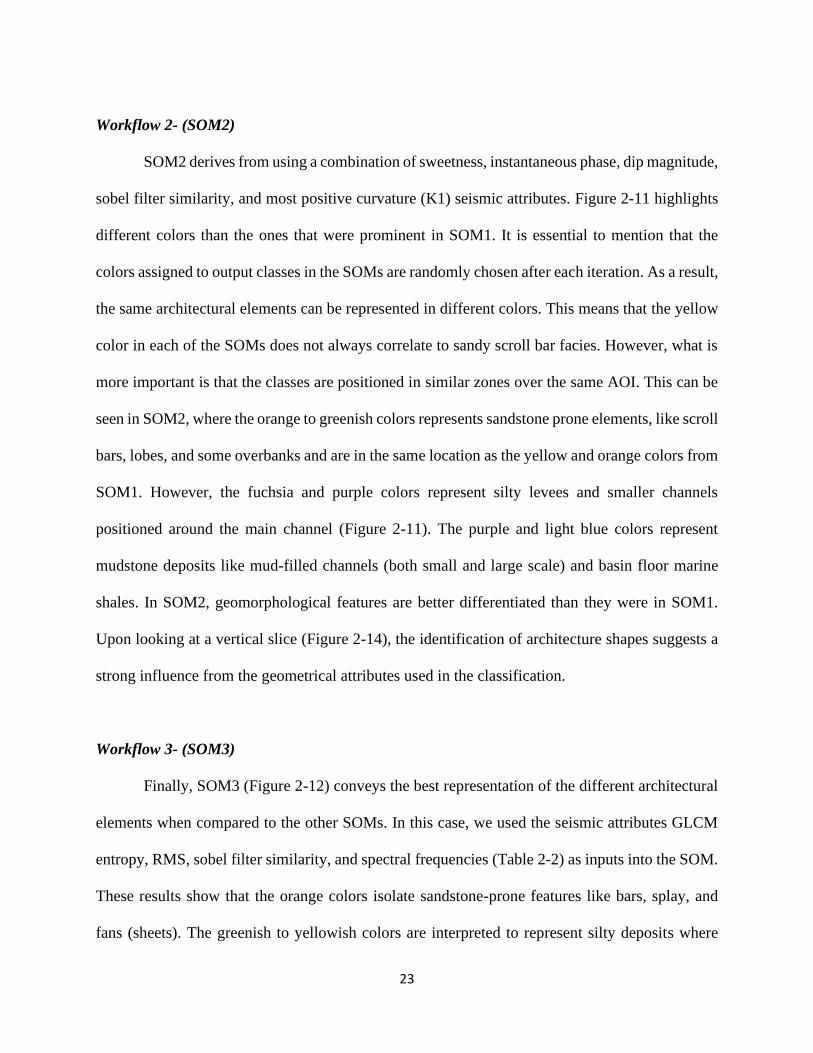
Workflow 2- (SOM2)
SOM2 derives from using a combination of sweetness, instantaneous phase, dip magnitude,
sobel filter similarity, and most positive curvature (K1) seismic attributes. Figure 2-11 highlights
different colors than the ones that were prominent in SOM1. It is essential to mention that the
colors assigned to output classes in the SOMs are randomly chosen after each iteration. As a result,
the same architectural elements can be represented in different colors. This means that the yellow
color in each of the SOMs does not always correlate to sandy scroll bar facies. However, what is
more important is that the classes are positioned in similar zones over the same AOI. This can be
seen in SOM2, where the orange to greenish colors represents sandstone prone elements, like scroll
bars, lobes, and some overbanks and are in the same location as the yellow and orange colors from
SOM1. However, the fuchsia and purple colors represent silty levees and smaller channels
positioned around the main channel (Figure 2-11). The purple and light blue colors represent
mudstone deposits like mud-filled channels (both small and large scale) and basin floor marine
shales. In SOM2, geomorphological features are better differentiated than they were in SOM1.
Upon looking at a vertical slice (Figure 2-14), the identification of architecture shapes suggests a
strong influence from the geometrical attributes used in the classification.
Workflow 3- (SOM3)
Finally, SOM3 (Figure 2-12) conveys the best representation of the different architectural
elements when compared to the other SOMs. In this case, we used the seismic attributes GLCM
entropy, RMS, sobel filter similarity, and spectral frequencies (Table 2-2) as inputs into the SOM.
These results show that the orange colors isolate sandstone-prone features like bars, splay, and
fans (sheets). The greenish to yellowish colors are interpreted to represent silty deposits where
24
sediment waves deposits are identified. The blue and purple classes help to identify the mud-filled
turbiditic channels (Figure 2-12) and basin floor marine shales. The purple color especially helps
to delineate the external geometry/geomorphology of features like levees. The SOM3 results
suggest that the combination of spectral and textural attributes further refine the classes identified
in the previous SOMs while also helping to resolve channels thicknesses that are slightly below
seismic resolution.
Testing results, time evolution, and architectural elements
After obtaining the SOMs and creating an interpretation of the deepwater system at the
time of the deposition of the Moki formation, we evaluated the SOM results. Figure 2-13 shows a
series of time slices that intersect the Pukeko-1 well, tied to the seismic volume. In the vertical
slice, we defined sample areas to evaluate the output classes from the SOM3 model. For example,
in the time slice taken at -1916 ms, the well has a low GR signature, which is characteristic of
shales. These characteristics are shown by the blue and purple colors in SOM3. However, in the
time slice taken at -1968 ms, there is a low GR value, which is characteristic of sandstones and
possesses a signature that is representative of a channel (blocky to finning upward log pattern).
This GR log feature is shown by the orange color in the SOM. In the other time slices that are
more mixed to- silty, the class is represented by green-yellowish color in SOM3. The well log
profiles matching the SOM results (Figure 2-13) allowed us to corroborate our analyses and be
able to make geological interpretations on the evolution of the system. These findings can be
further used to determine volumetric estimations of these reservoirs or seismic facies of interest.
In this instance, the seismic data shows how the geomorphology of the channel complexes change
upwards, from straight-linear (most likely channelized gullies) to a higher sinuosity, meandering
25
character (channel-levee complexes). The channel widths also vary from ~200 m to 5 km for these
channel complexes. This suggests that there were changes in the energy, slope, and trigger factors
(Catuneanu, 2009) within the Miocene deepwater system, having individual older channels
followed by younger channel complexes.
After looking at vertical slices and time slices, it seemed that the sandy-prone facies were
predominant in the lower time slices, and the system becomes more mud-rich up section. We
interpret the system in our section of interest to be a channelized turbidite fan system where the
channels became progressively more carved and migrated laterally due to avulsion. Additionally,
the deposits that were reworked by bottom currents, as suggested by Kroeger et al., (2019), were
recognized in the horizon slices with the aid of the SOM results. Single attributes did not allow for
the recognition of these features.
Figure 2-14 presents the SOM results in a vertical slice. When comparing SOM1, SOM2,
and SOM3, in general, sandy-prone facies (channels and fans) are located relatively in the same
position (in time/ vertically). The mud-prone facies, recognized as the basin-floor marine shales,
are positioned in similar areas in the three SOMs cases. SOM3 (Figure 2-15) appears to present
more details and classes than the other two SOM results. Therefore, it suggests that the
incorporation of textural and spectral attributes generates a more robust classification of the
deepwater facies.
DISCUSSION
A clear understanding of the dataset and the establishment of a geological goal is
paramount. This is the first step we recommend before any multi-attribute analysis or machine
learning application. By establishing a clear objective, the interpreter can incorporate the attributes
that can represent the most meaningful information based on the available data. In the case of this
26
study, only a PSTM volume is available. Thus, we can only generate spectral, geometric, textural,
and instantaneous attributes. These attributes help define the geomorphological properties of
deepwater architectural elements while also providing an understand of their possible lithologies
as presented in the SOM results. Chopra and Marfurt (2014) highlighted the importance of using
different types of attributes in order to capture both structural and stratigraphic features present
within the dataset. The incorporation of multiple attributes types as input for SOM studies to
enhance seismic interpretation has become a common practice, as observed by Sacrey and Roden
(2014) and by Roden and Sacrey (2016). These studies are the first step in the right direction for
efficient and robust seismic characterization.
The selection of the attributes considered the findings presented in Barnes (2007) and Kim
(2019). When selecting the appropriate attribute combinations, we discarded the GLCM
homogeneity attribute as it shared a redundant classification with the GLCM entropy attribute
(e.g., an R value greater than 0.7).
We corroborated that the sweetness and RMS amplitude seismic attributes are good
lithological indicators. The higher the values of these two attributes, the more sand-prone the facies
are, as can be seen in Figures 2-7a and 2-8b. On the other hand, seismic attributes, such as
coherence and dip magnitude, highlight the geomorphology of the architectural elements within
the channel belt complex. This can be seen in the various channels, levees, scroll bars, splays/
overbank, and abandoned channel features present in Figure 2-8c. Most positive curvature (k1)
excels in identifying the positive relief created by levees when compared to the other attributes
(Figure 2-7e).
Although each seismic attribute provides individual hints about the facies and the
geomorphology of the deepwater elements, this study demonstrates that SOMs create a more
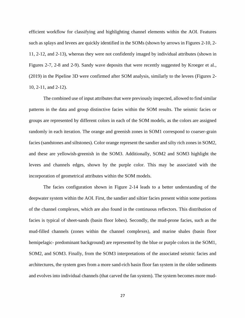
27
efficient workflow for classifying and highlighting channel elements within the AOI. Features
such as splays and levees are quickly identified in the SOMs (shown by arrows in Figures 2-10, 2-
11, 2-12, and 2-13), whereas they were not confidently imaged by individual attributes (shown in
Figures 2-7, 2-8 and 2-9). Sandy wave deposits that were recently suggested by Kroeger et al.,
(2019) in the Pipeline 3D were confirmed after SOM analysis, similarly to the levees (Figures 2-
10, 2-11, and 2-12).
The combined use of input attributes that were previously inspected, allowed to find similar
patterns in the data and group distinctive facies within the SOM results. The seismic facies or
groups are represented by different colors in each of the SOM models, as the colors are assigned
randomly in each iteration. The orange and greenish zones in SOM1 correspond to coarser-grain
facies (sandstones and siltstones). Color orange represent the sandier and silty rich zones in SOM2,
and these are yellowish-greenish in the SOM3. Additionally, SOM2 and SOM3 highlight the
levees and channels edges, shown by the purple color. This may be associated with the
incorporation of geometrical attributes within the SOM models.
The facies configuration shown in Figure 2-14 leads to a better understanding of the
deepwater system within the AOI. First, the sandier and siltier facies present within some portions
of the channel complexes, which are also found in the continuous reflectors. This distribution of
facies is typical of sheet-sands (basin floor lobes). Secondly, the mud-prone facies, such as the
mud-filled channels (zones within the channel complexes), and marine shales (basin floor
hemipelagic- predominant background) are represented by the blue or purple colors in the SOM1,
SOM2, and SOM3. Finally, from the SOM3 interpretations of the associated seismic facies and
architectures, the system goes from a more sand-rich basin floor fan system in the older sediments
and evolves into individual channels (that carved the fan system). The system becomes more mud-
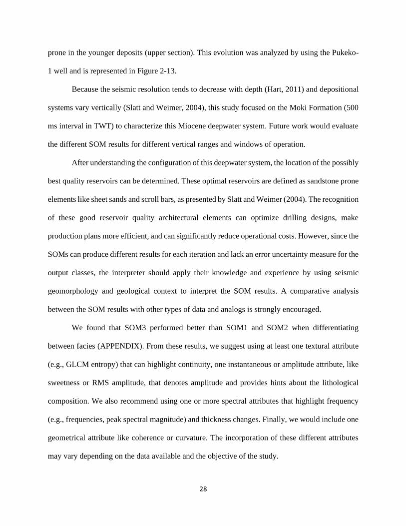
28
prone in the younger deposits (upper section). This evolution was analyzed by using the Pukeko-
1 well and is represented in Figure 2-13.
Because the seismic resolution tends to decrease with depth (Hart, 2011) and depositional
systems vary vertically (Slatt and Weimer, 2004), this study focused on the Moki Formation (500
ms interval in TWT) to characterize this Miocene deepwater system. Future work would evaluate
the different SOM results for different vertical ranges and windows of operation.
After understanding the configuration of this deepwater system, the location of the possibly
best quality reservoirs can be determined. These optimal reservoirs are defined as sandstone prone
elements like sheet sands and scroll bars, as presented by Slatt and Weimer (2004). The recognition
of these good reservoir quality architectural elements can optimize drilling designs, make
production plans more efficient, and can significantly reduce operational costs. However, since the
SOMs can produce different results for each iteration and lack an error uncertainty measure for the
output classes, the interpreter should apply their knowledge and experience by using seismic
geomorphology and geological context to interpret the SOM results. A comparative analysis
between the SOM results with other types of data and analogs is strongly encouraged.
We found that SOM3 performed better than SOM1 and SOM2 when differentiating
between facies (APPENDIX). From these results, we suggest using at least one textural attribute
(e.g., GLCM entropy) that can highlight continuity, one instantaneous or amplitude attribute, like
sweetness or RMS amplitude, that denotes amplitude and provides hints about the lithological
composition. We also recommend using one or more spectral attributes that highlight frequency
(e.g., frequencies, peak spectral magnitude) and thickness changes. Finally, we would include one
geometrical attribute like coherence or curvature. The incorporation of these different attributes
may vary depending on the data available and the objective of the study.
29
Machine learning algorithms can serve as a tool for assisting seismic interpreters by
identifying relationships within the data that humans may not be able to recognize easily. However,
the interpreter is vital for either training the algorithms or for interpreting the results within a
geological context, which is something that these algorithms cannot yet accomplish.
CONCLUSIONS
In this study, we tested a wide range of geometrical, spectral, instantaneous, and textural
attributes, and we later incorporated the chosen combinations into three different SOM models to
enhance deepwater architectural elements and facies interpretations. For that, we tested the
deepwater Moki Formation within the Pipeline 3D dataset located in the Taranaki Basin.
The first takeaway of the study is that the establishment of a clear goal is paramount before
any seismic interpretation study. The interpreter should first inspect the seismic dataset to
recognize noise and define the goal. Then, the interpreter would be able to select the most suitable
(geologically meaningful) attributes for the dataset and the study objective. For the pre-selection
of candidate attributes, we suggest to use a combination of 1) at least one geometrical attribute that
defines the geomorphology of the architectural elements (e.g., sobel filter similarity), 2) one
amplitude attribute like RMS or sweetness for accentuating sand-prone facies and architectures
(e.g., sand-filled channels, lobes or sheet sands); and 3) at least one textural attribute such as
GLCM entropy to differentiate facies (e.g., MTD from mud-filled channels). In addition to this,
the combination of attributes should have a non-linear relation among them to avoid redundancy.
The use of spectral attributes and curvature in our dataset resulted beneficial in discriminating
elements like levees (positive curvature, high spectral frequency) from major dimension
architectures like channels (low spectral frequency).
30
When comparing the three SOMs based on the different combinations, we found that
SOM3 offered better detail that allowed us to interpret smaller features like levees, sand waves,
and smaller channels. The robustness of these results may be attributed to the use of individual
spectral frequencies in addition to the GLCM entropy attribute.
Whereas each seismic attribute provides hints about facies and geomorphology, we
demonstrated that the application of SOMs allows for a more efficient workflow in deepwater
element discrimination and classification (e.g., splays, levees, and smaller features). Machine
learning techniques like SOMs allow for multiple attributes to be combined and to extract
meaningful information from the seismic samples (when the user can just recognize limited
patterns or features). If attributes are tested to be meaningful before the application of any
clustering algorithm, we may get a more robust classification. We must remember that the
machines cannot (yet) inherit our knowledge and criteria. Therefore, the goal of the project, the
interpreter experience and “in context” interpretations play a key role in using unsupervised
machine learning techniques for seismic facies interpretation
ACKNOWLEDGMENTS
We acknowledge New Zealand Petroleum and Minerals for providing the dataset used for
this research. We thank the AASPI consortium for the access to AASPI (attribute assisted seismic
processing and interpretation). In the same way, we extend our appreciation to Schlumberger for
the Petrel license. They provided these licenses to the University of Oklahoma for research and
education purposes. We also thank Julian Chenin for his support. Special appreciation is dedicated
to Dr. Kurt Marfurt, Javier Tellez, and Dr. Rafael Pires de Lima for their valuable contribution and
advice throughout the research.
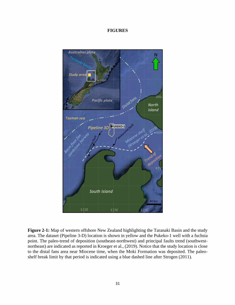
31
FIGURES
Figure 2-1: Map of western offshore New Zealand highlighting the Taranaki Basin and the study
area. The dataset (Pipeline 3-D) location is shown in yellow and the Pukeko-1 well with a fuchsia
point. The paleo-trend of deposition (southeast-northwest) and principal faults trend (southwest-
northeast) are indicated as reported in Kroeger et al., (2019). Notice that the study location is close
to the distal fans area near Miocene time, when the Moki Formation was deposited. The paleo-
shelf break limit by that period is indicated using a blue dashed line after Strogen (2011).
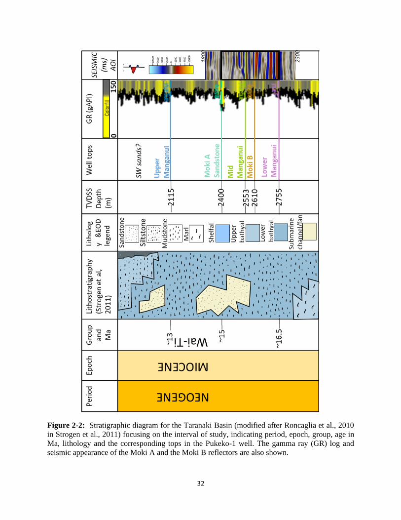
32
Figure 2-2: Stratigraphic diagram for the Taranaki Basin (modified after Roncaglia et al., 2010
in Strogen et al., 2011) focusing on the interval of study, indicating period, epoch, group, age in
Ma, lithology and the corresponding tops in the Pukeko-1 well. The gamma ray (GR) log and
seismic appearance of the Moki A and the Moki B reflectors are also shown.
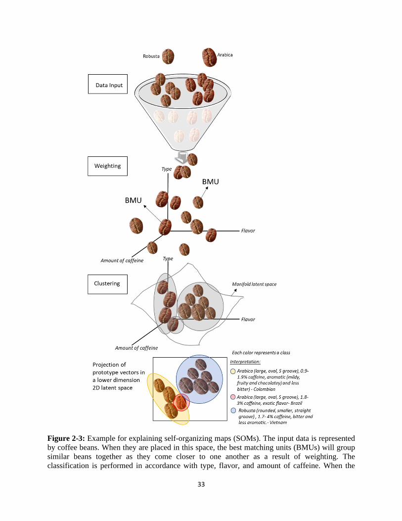
33
Figure 2-3: Example for explaining self-organizing maps (SOMs). The input data is represented
by coffee beans. When they are placed in this space, the best matching units (BMUs) will group
similar beans together as they come closer to one another as a result of weighting. The
classification is performed in accordance with type, flavor, and amount of caffeine. When the
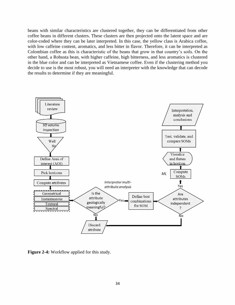
34
beans with similar characteristics are clustered together, they can be differentiated from other
coffee beans in different clusters. These clusters are then projected onto the latent space and are
color-coded where they can be later interpreted. In this case, the yellow class is Arabica coffee,
with low caffeine content, aromatics, and less bitter in flavor. Therefore, it can be interpreted as
Colombian coffee as this is characteristic of the beans that grow in that country’s soils. On the
other hand, a Robusta bean, with higher caffeine, high bitterness, and less aromatics is clustered
in the blue color and can be interpreted as Vietnamese coffee. Even if the clustering method you
decide to use is the most robust, you will need an interpreter with the knowledge that can decode
the results to determine if they are meaningful.
Figure 2-4: Workflow applied for this study.
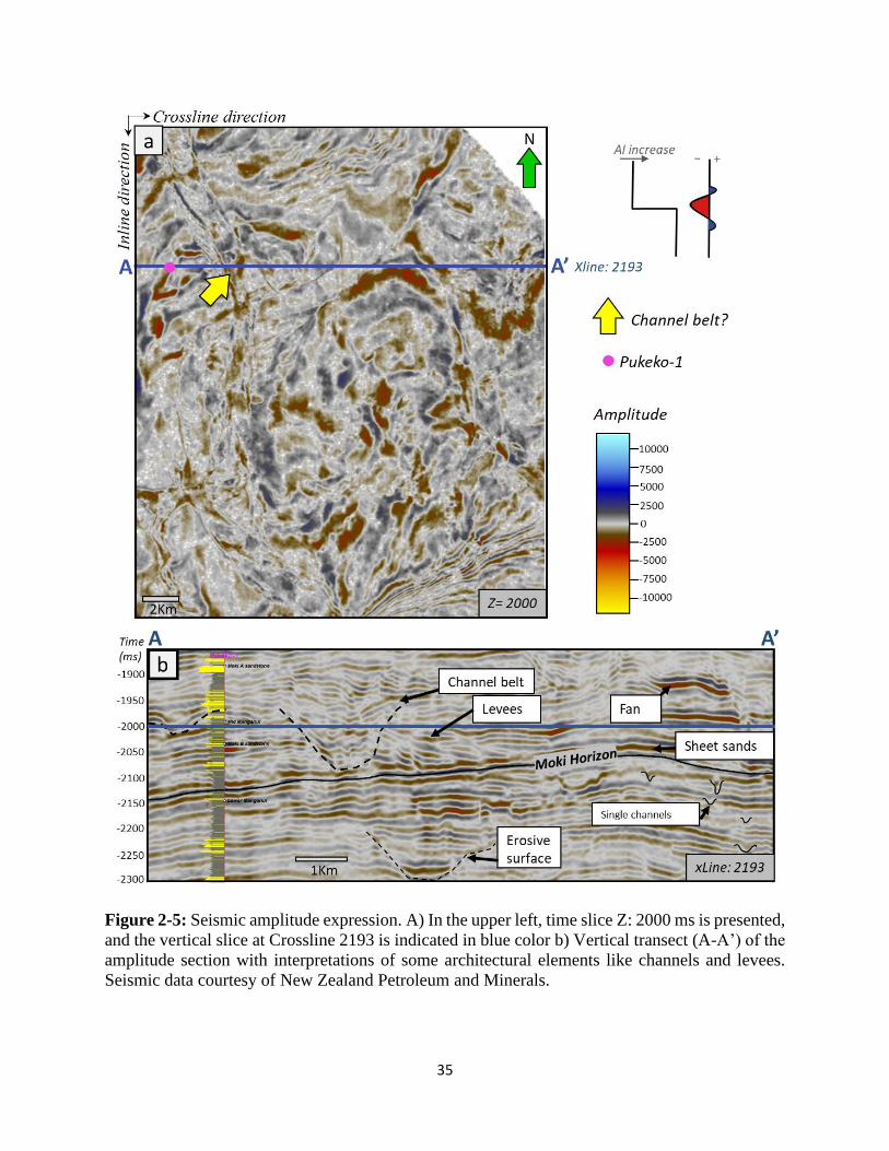
35
Figure 2-5: Seismic amplitude expression. A) In the upper left, time slice Z: 2000 ms is presented,
and the vertical slice at Crossline 2193 is indicated in blue color b) Vertical transect (A-A’) of the
amplitude section with interpretations of some architectural elements like channels and levees.
Seismic data courtesy of New Zealand Petroleum and Minerals.
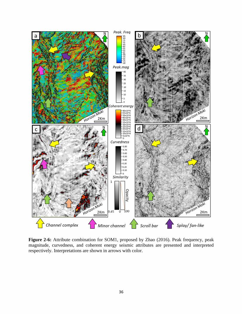
36
Figure 2-6: Attribute combination for SOM1, proposed by Zhao (2016). Peak frequency, peak
magnitude, curvedness, and coherent energy seismic attributes are presented and interpreted
respectively. Interpretations are shown in arrows with color.
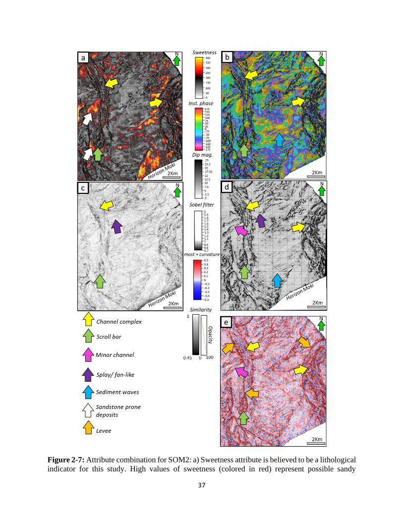
37
Figure 2-7: Attribute combination for SOM2: a) Sweetness attribute is believed to be a lithological
indicator for this study. High values of sweetness (colored in red) represent possible sandy
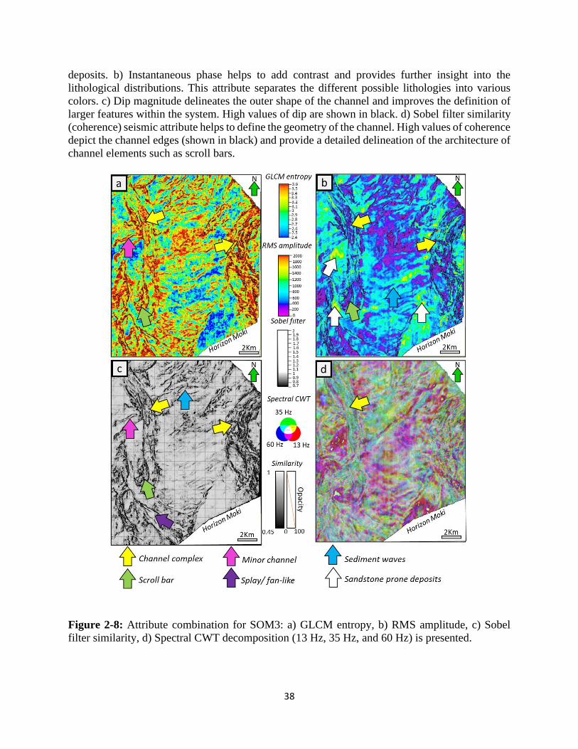
38
deposits. b) Instantaneous phase helps to add contrast and provides further insight into the
lithological distributions. This attribute separates the different possible lithologies into various
colors. c) Dip magnitude delineates the outer shape of the channel and improves the definition of
larger features within the system. High values of dip are shown in black. d) Sobel filter similarity
(coherence) seismic attribute helps to define the geometry of the channel. High values of coherence
depict the channel edges (shown in black) and provide a detailed delineation of the architecture of
channel elements such as scroll bars.
Figure 2-8: Attribute combination for SOM3: a) GLCM entropy, b) RMS amplitude, c) Sobel
filter similarity, d) Spectral CWT decomposition (13 Hz, 35 Hz, and 60 Hz) is presented.
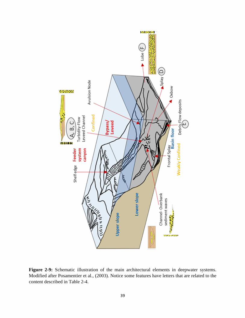
39
Figure 2-9: Schematic illustration of the main architectural elements in deepwater systems.
Modified after Posamentier et al., (2003). Notice some features have letters that are related to the
content described in Table 2-4.
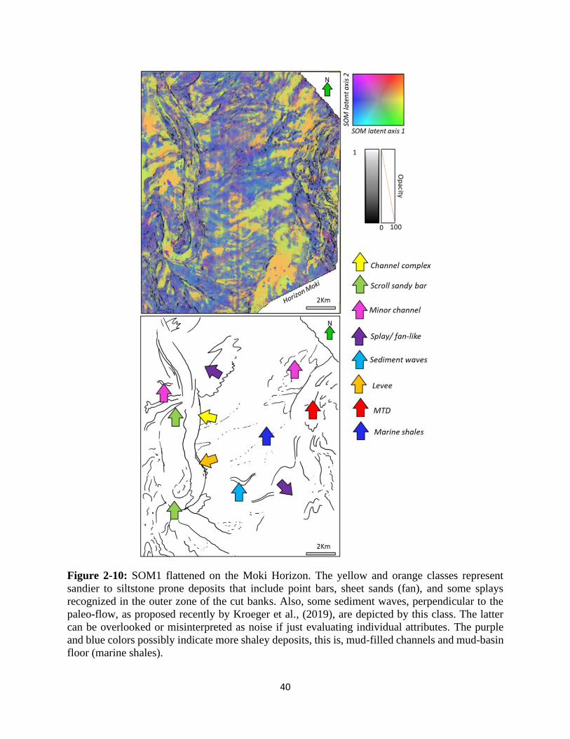
40
Figure 2-10: SOM1 flattened on the Moki Horizon. The yellow and orange classes represent
sandier to siltstone prone deposits that include point bars, sheet sands (fan), and some splays
recognized in the outer zone of the cut banks. Also, some sediment waves, perpendicular to the
paleo-flow, as proposed recently by Kroeger et al., (2019), are depicted by this class. The latter
can be overlooked or misinterpreted as noise if just evaluating individual attributes. The purple
and blue colors possibly indicate more shaley deposits, this is, mud-filled channels and mud-basin
floor (marine shales).
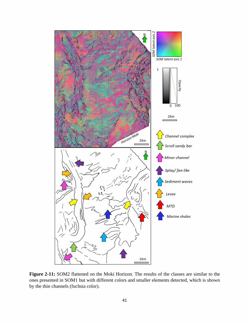
41
Figure 2-11: SOM2 flattened on the Moki Horizon. The results of the classes are similar to the
ones presented in SOM1 but with different colors and smaller elements detected, which is shown
by the thin channels (fuchsia color).
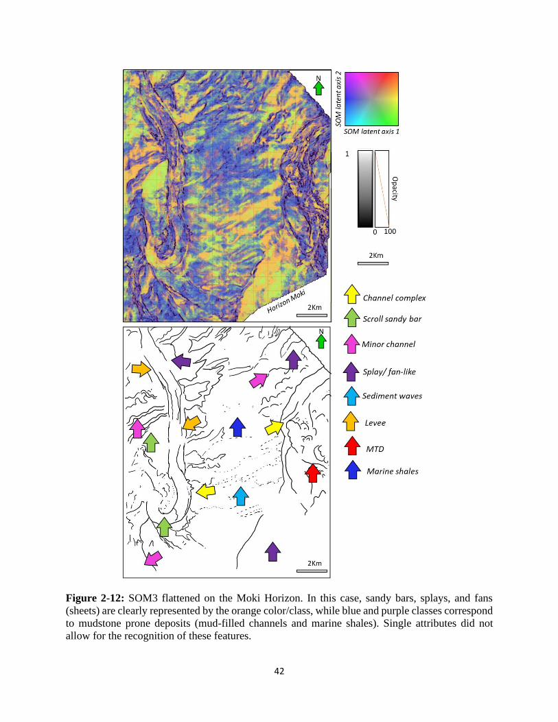
42
Figure 2-12: SOM3 flattened on the Moki Horizon. In this case, sandy bars, splays, and fans
(sheets) are clearly represented by the orange color/class, while blue and purple classes correspond
to mudstone prone deposits (mud-filled channels and marine shales). Single attributes did not
allow for the recognition of these features.
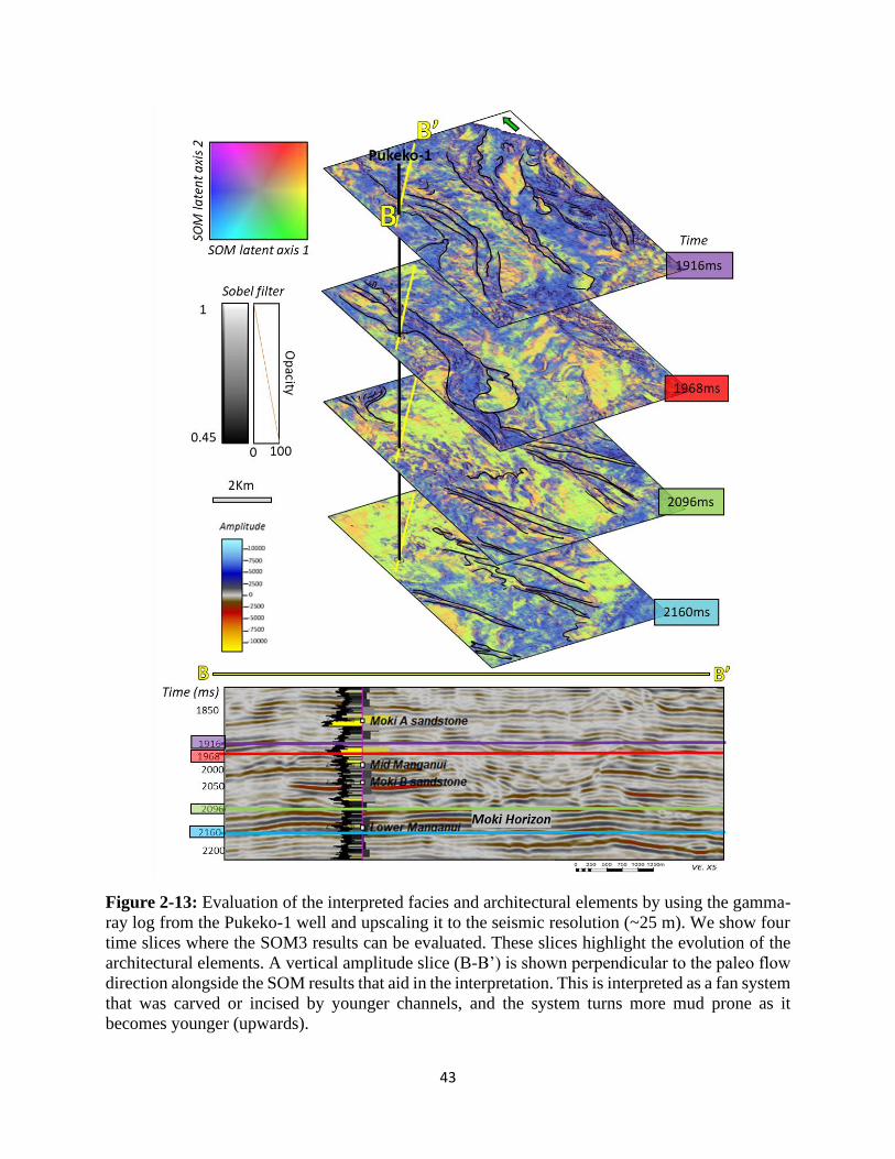
43
Figure 2-13: Evaluation of the interpreted facies and architectural elements by using the gamma-
ray log from the Pukeko-1 well and upscaling it to the seismic resolution (~25 m). We show four
time slices where the SOM3 results can be evaluated. These slices highlight the evolution of the
architectural elements. A vertical amplitude slice (B-B’) is shown perpendicular to the paleo flow
direction alongside the SOM results that aid in the interpretation. This is interpreted as a fan system
that was carved or incised by younger channels, and the system turns more mud prone as it
becomes younger (upwards).
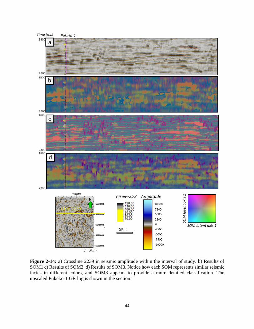
44
Figure 2-14: a) Crossline 2239 in seismic amplitude within the interval of study. b) Results of
SOM1 c) Results of SOM2, d) Results of SOM3. Notice how each SOM represents similar seismic
facies in different colors, and SOM3 appears to provide a more detailed classification. The
upscaled Pukeko-1 GR log is shown in the section.
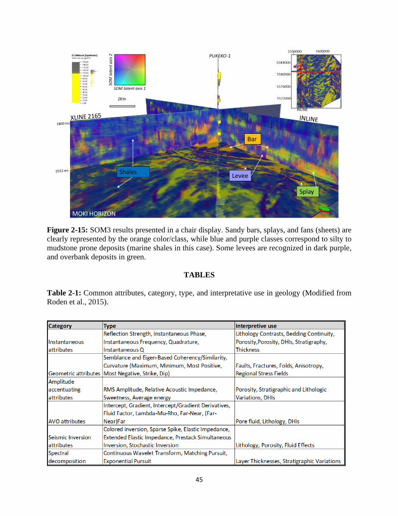
45
Figure 2-15: SOM3 results presented in a chair display. Sandy bars, splays, and fans (sheets) are
clearly represented by the orange color/class, while blue and purple classes correspond to silty to
mudstone prone deposits (marine shales in this case). Some levees are recognized in dark purple,
and overbank deposits in green.
TABLES
Table 2-1: Common attributes, category, type, and interpretative use in geology (Modified from
Roden et al., 2015).
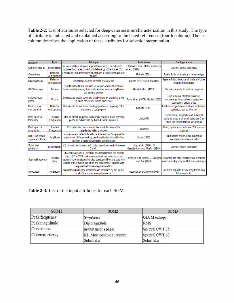
46
Table 2-2: List of attributes selected for deepwater seismic characterization in this study. The type
of attribute is indicated and explained according to the listed references (fourth column). The last
column describes the application of these attributes for seismic interpretation.
Table 2-3: List of the input attributes for each SOM.
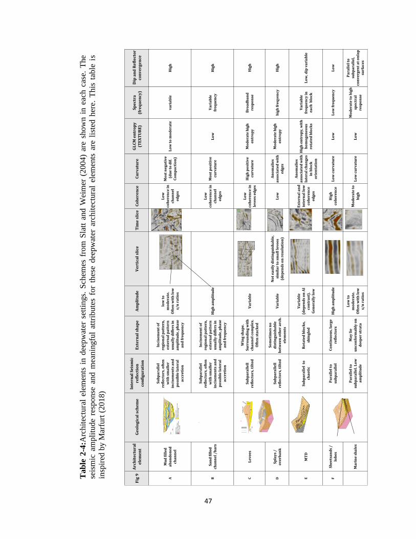
47
Fig
9A
rch
ite
ctu
ral
ele
me
nt
Ge
olo
gic
al
sch
em
eIn
tern
al
Seis
mic
re
fle
ctio
n
con
fig
ura
tio
nE
xte
rna
l sh
ap
eA
mp
litu
de
V
ert
ica
l sl
ice
Tim
e s
lice
Co
he
ren
ceC
urv
atu
reG
LC
M e
ntr
op
y
(TE
XT
UR
E)
Spe
ctra
(f
req
ue
ncy
) D
ip a
nd
Re
fle
cto
r co
nv
erg
en
ce
A
Mu
d f
ille
d
ab
an
do
ne
d
cha
nn
el
Su
bp
ara
lle
l re
fle
cto
rs, o
fte
n
wit
h s
ma
lle
r in
cise
me
nts
an
d
po
ssib
le l
ate
ral
acc
reti
on
Inci
sem
en
t o
f re
gio
na
l p
att
ern
, e
xte
rna
l p
att
ern
u
sua
lly
dif
fers
in
a
mp
litu
de
, ph
ase
a
nd
fre
qu
en
cy
low
to
m
od
era
te.
Oft
en
wit
h l
ow
s/
n r
ati
os
Lo
w
coh
ere
nce
in
ch
an
ne
l e
dg
es
Mo
st n
eg
ati
ve
(d
ue
to
dif
. C
om
pa
ctio
n)
Lo
w t
o m
od
era
tev
ari
ab
leH
igh
BS
an
d f
ille
d
cha
nn
el
/b
ars
Su
bp
ara
lle
l re
fle
cto
rs, o
fte
n
wit
h s
ma
lle
r in
cise
me
nts
an
d
po
ssib
le l
ate
ral
acc
reti
on
Inci
sem
en
t o
f re
gio
na
l p
att
ern
, e
xte
rna
l p
att
ern
u
sua
lly
dif
fers
in
a
mp
litu
de
, ph
ase
a
nd
fre
qu
en
cy
Hig
h a
mp
litu
de
Lo
w
coh
ere
nce
in
ch
an
ne
l e
dg
es
Mo
st p
osi
tiv
e
curv
atu
reL
ow
Va
ria
ble
fr
eq
ue
ncy
H
igh
CL
ev
ee
sS
ub
pa
rall
ell
re
fle
cto
rs, t
ilte
d
Win
g s
ha
pe
. S
urr
ou
nd
ing
wit
h
cha
nn
el
com
ple
x.
Oft
en
sta
cke
d
Va
ria
ble
Lo
w
coh
ere
nce
in
le
ve
es
ed
ge
s
Hig
h p
osi
tiv
e
curv
atu
reM
od
era
te h
igh
e
ntr
op
yB
roa
db
an
d
resp
on
seH
igh
DS
pla
ys
/
ov
erb
an
kS
ub
pa
rall
ell
re
fle
cto
rs, t
ilte
d
So
me
tim
es
no
d
isti
ng
uis
ha
ble
b
etw
ee
n o
the
r a
rch
. e
lem
en
ts
Va
ria
ble
No
t e
asi
ly d
isti
ng
uis
ha
ble
, si
mil
ar
to s
ma
ll l
ev
ee
s (d
ep
en
ds
on
re
solu
tio
n)
Lo
wA
no
ma
lie
s a
sso
cia
ted
wit
h
ed
ge
s
Mo
de
rate
hig
h
en
tro
py
hig
h f
req
ye
ncy
Hig
h
EM
TD
Su
bp
ara
lle
l t
o
cha
oti
cR
ota
ted
blo
cks,
sh
ing
led
Va
ria
ble
(d
ep
en
ds
on
AI
con
tra
st).
G
en
era
lly
lo
w
Ex
tern
al
an
d
inte
rna
l lo
w
coh
ere
nce
e
dg
es
An
om
ali
es
ass
oci
ate
d w
ith
la
tera
l ch
an
ge
s in
blo
ck
ori
en
tati
on
Hig
h e
ntr
op
y, w
ith
h
om
og
en
eo
us
rota
ted
blo
cks
Va
ria
ble
fr
eq
ue
ncy
in
e
ach
blo
ckL
ow
, dip
va
ria
ble
FS
he
ets
an
ds
/
lob
es
Pa
rall
el
to
sub
pa
rall
el
Co
nti
nu
ou
s, l
arg
e
refl
ect
ors
Hig
h a
mp
litu
de
Hig
h
coh
ere
nce
Lo
w c
urv
atu
reL
ow
Lo
w f
req
ue
ncy
Lo
w
Ma
rin
e s
ha
les
Pa
rall
el
to
sub
pa
rall
el.
Lo
w
am
pli
tud
e
Ma
y l
ie
un
con
form
ab
ly o
n
de
ep
er
stra
ta
Lo
w t
o
mo
de
rate
. O
fte
n w
ith
lo
w
s/n
ra
tio
s
Mo
de
rate
to
h
igh
Lo
w c
urv
atu
reL
ow
Mo
de
rate
to
hig
h
spe
ctra
l re
spo
nse
Pa
rall
el
to
sub
pa
rall
el,
co
nv
erg
en
t a
t o
nla
p
surf
ace
s
Inli
ne
Z
Tab
le 2
-4:A
rchit
ectu
ral
elem
ents
in d
eepw
ater
set
tings.
Sch
emes
fro
m S
latt
and W
eim
er (
2004)
are
show
n i
n e
ach c
ase.
The
seis
mic
am
pli
tude
resp
onse
and m
eanin
gfu
l at
trib
ute
s fo
r th
ese
dee
pw
ater
arc
hit
ectu
ral
elem
ents
are
lis
ted h
ere.
This
tab
le i
s
insp
ired
by M
arfu
rt (
201
8)
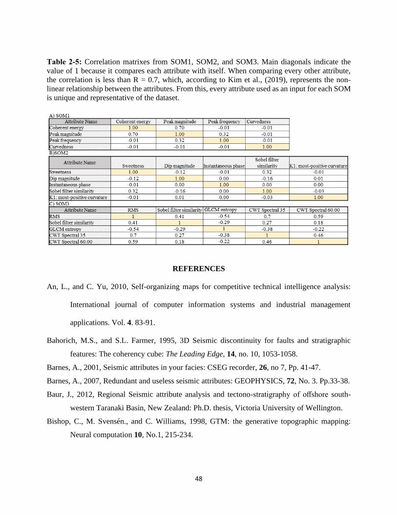
48
Table 2-5: Correlation matrixes from SOM1, SOM2, and SOM3. Main diagonals indicate the
value of 1 because it compares each attribute with itself. When comparing every other attribute,
the correlation is less than R = 0.7, which, according to Kim et al., (2019), represents the non-
linear relationship between the attributes. From this, every attribute used as an input for each SOM
is unique and representative of the dataset.
REFERENCES
An, L., and C. Yu, 2010, Self-organizing maps for competitive technical intelligence analysis:
International journal of computer information systems and industrial management
applications. Vol. 4. 83-91.
Bahorich, M.S., and S.L. Farmer, 1995, 3D Seismic discontinuity for faults and stratigraphic
features: The coherency cube: The Leading Edge, 14, no. 10, 1053-1058.
Barnes, A., 2001, Seismic attributes in your facies: CSEG recorder, 26, no 7, Pp. 41-47.
Barnes, A., 2007, Redundant and useless seismic attributes: GEOPHYSICS, 72, No. 3. Pp.33-38.
Baur, J., 2012, Regional Seismic attribute analysis and tectono-stratigraphy of offshore south-
western Taranaki Basin, New Zealand: Ph.D. thesis, Victoria University of Wellington.
Bishop, C., M. Svensén., and C. Williams, 1998, GTM: the generative topographic mapping:
Neural computation 10, No.1, 215-234.
49
Bull, S., A. Nicol., D.P. Strogen., K.F. Kroeger., and H. Seebeck, 2018, Tectonic controls on
sedimentation in the Southern Taranaki Basin during the Miocene and implications for
New Zealand plate boundary deformation: Basin Research, 31, 2.
Castagna, J.P., and S. Sun, 2006, Comparison of spectral decomposition methods: First Break, 24,
75-79.
Catuneanu, O., V. Abreu., J.P. Bhattacharya et al., 2009, Towards the standardization of sequence
stratigraphy: Earth-science reviews, 92, Elsevier. Pp. 1-33.
Chopra, S; and K. J. Marfurt, 2007, Seismic attributes for prospect identification and reservoir
characterization: Society of exploration geophysicists.
Chopra, S; and K. J. Marfurt, 2014, Churning seismic attributes with principal component analysis:
86th annual international meeting, SEG, Expanded abstracts 2672-2676.
Coleou, T., M. Poupon., and K. Azbel, 2003, Unsupervised seismic facies classification: A review
and comparison of techniques and implementation: The Leading Edge, 22, 942–953.
Forgy, E.W. (1965) Cluster Analysis of Multivariate Data: Efficiency vs Interpretability of
Classifications. Biometrics, 21, 768-780.Gao, D., 2007, Application of three-dimensional
seismic texture analysis with special reference to deep-marine facies discrimination and
interpretation: An example from offshore Angola, West Africa: AAPG Bulletin, 91, 1665-
1683.
Gersztenkorn, A., and K.J. Marfurt, 1999, Eigenstructure based coherence computations as an aid
to 3D structural and stratigraphic mapping: GEOPHYSICS, 64, no.5, 1468-1479.
Gibson, P.B., S.E.Perkins-Kirkpatrick., P. Uotila., A.S.Pepler., and L.V.Alexander, 2017, On the
use of self-organizing maps for studying climate extremes: Geophys. Res. Atomos., 122,
3891-3903, doi: 1.0.1002/2016JD0262256.
Hanafizadeh, P., and M. Mirzazadeh, 2010, Visualizing market segmentation using self-organizing
maps and fuzzy delphi method- ADSL market of a telecommunication company. Expert
systems with applications 38, Elsevier. 198-205
Hart, B, 2011, Introduction to seismic interpretation. AAPG discovery series No.16.
Hartigan. H, 1975, Clustering Algorithms. John Wiley & Sons.
Haralick, R.M., K. Shanmugam., and I. Dinstein, 1973, Textural features for image classification:
Institute of electrical and electronic engineers’ transactions on systems, man and
cybernetics: SMC, 3, 610-621.
50
Holt, W.E., and T.A. Stern., 1994, Subduction, platform subsidence, and foreland thrust
loading: the late Tertiary development of Taranaki Basin, New Zealand: Tectonics 13 (5), 1068–
1092.
Infante-Paez, L., and K.J. Marfurt, 2019, Using machine learning as an aid to seismic
geomorphology, which attributes are the best input? Interpretation, 7 (3), SE1-SE18.
Kim, Y., R. Hardisty., and K.J. Marfurt., 2019. Attribute selection in seismic facies classification:
application to a Gulf of Mexico 3D seismic survey and the Barnett Shale: Interpretation,
7 (3), 281-297.
King, P.R., and G.P. Thrasher, 1996, Cretaceous-Cenozoic geology and petroleum systems of the
Taranaki Basin, New Zealand: Institute of Geological and Nuclear Sciences Monograph,
pp. 243.
King, P.R, 2000, New Zealand's changing configuration in the last 100 million years: plate
tectonics, basin development, and depositional setting: New Zealand Oil Exploration
Conference Proceedings. Ministry of Economic Development, Wellington, pp. 132–146.
Kohonen, T, 1982, Self-organized formation of topologically correct feature maps: Biological
cybernetics, 43, 59-69.
Kohonen, T, 1995, Self-organizing maps. In Springer Series in Information Sciences (Vol. 30).
Berlin, Heidelberg, New York: Springer.
Kroeger, K.F., G.P. Thrasher., and M. Sarma, 2019, The evolution of a Middle Miocene deep-
water sedimentary system in northwestern New Zealand (Taranaki Basin) depositional
controls and mechanisms: Marine and Petroleum Geology, 101, 355-372.
La Marca-Molina, K., C. Silver., H.Bedle., and R. Slatt, 2019. Seismic facies identification in a
deepwater channel complex applying seismic attributes and unsupervised machine learning
techniques. A case study in the Taranaki Basin, New Zealand: 89th annual international
meeting, SEG, Expanded abstracts, 2059-2063.
Liu, J, and K.J. Marfurt, 2007, Instantaneous spectral attributes to detect channels. GEOPHYSICS,
72, NO.2; P23-P31
Luo, Y., W.G. Higgs, and S. Kowalik, 1996, Edge detection and stratigraphic analysis using 3-D
seismic data: 66th annual meeting, SEG, Expanded abstracts, 324-327.
Macrae, E. J., C. E. Bond, Z. K. Shipton., and R. J. Lunn, 2016, Increasing the quality of seismic
interpretation: Interpretation, 4, no. 3, T395–T402
51
Marfurt, K.J, 2006, Robust estimates of reflector dip and azimuth: GEOPHYSICS, 71, no. 4, P29-
P40.
Marfurt, K.J, 2018, Seismic attributes as the framework for data integration throughout the oilfield
life cycle. 2018 Distinguished instructor short course. Distinguished instructor series, No.
21: Society of Exploration Geophysicists.
Meek, T, 2013, Applications of 3D seismic attribute analysis workflows: a case study from Ness
County, Kansas, USA, MSc. Thesis, Kansas State University.
New Zealand Petroleum & Minerals, 2014, New Zealand petroleum basins. Ministry of Business,
Innovation & Employment.
Partyka, G., J. Gridley, and J. A. Lopez, 1999, Interpretational applications of spectral
decomposition in reservoir characterization: The leading Edge, 18, no. 3, 353-360.
Pearson, K, 1901, On lines and planes of closest fit to systems of points in space. Phil. Mag. (6),
2, 559–572
Pires de Lima, R., 2019, Machine learning applications for geoscience problems: Ph.D. thesis,
University of Oklahoma.
Posamentier, H.W., and V. Kolla, 2003, Seismic geomorphology and stratigraphy of depositional
elements in deep-water settings: Journal of Sedimentary Research, 73, 367-388.
Posamentier, H.W., and V, O. Martinsen, 2010, The character and genesis of submarine mass-
transport deposits: insights from outcrop and 3D seismic data: SEPM Special Publication
No. 95.
Posamentier, H, 2015, Application of 3D seismic visualization techniques for seismic stratigraphy,
seismic geomorphology, and depositional systems analysis: examples from fluvial to deep-
marine depositional environments: in Dore, A., and B.A. Vinning. (eds) Petroleum
geology: North-West Europe and global perspectives- proceedings of the 6th petroleum
geology conference, 1565-1576. Geological Society, London.
Prather, B.F., F.B. Keller., and M.A. Chapin, 2000, Hierarchy of deep-water architectural elements
with reference to seismic resolution: Implications for reservoir prediction and modeling
depositional systems. In: Weimer, P., R.M. Sian., J.L. Coleman., N. Rosen., A.H. Bouma,
et al., (Eds.), Global Deep-Water Reservoirs: Gulf Coast Section SFPM Foundation 20th
Annual Bob F Perkins Research Conference, pp. 817–835
52
Radovich, B. J, and R.B. Oliveros, 1998, 3-D sequence interpretation of seismic instantaneous
attributes from the Gorgon field: The Leading Edge, 17, 1286-1293.
Roberts, A, 2001, Curvature attributes and their application to 3D interpreted horizons: First Break,
19, no. 2, 85-100.
Roden, R., T. Smith., and D. Sacrey, 2015, Geologic pattern recognition from seismic attributes:
Principal component analysis and self-organizing map: Interpretation, 3, SAE59–SAE83.
Roden, R., and D. Sacrey, 2016, Seismic interpretation with machine learning: GeoExpro. Vol 13.
No 6. pp 50-53
Roy, A, 2013, Latent space classification of seismic facies: Ph.D. dissertation, University of
Oklahoma.
Russell, B., and D. Hampson, 1997, Multiattribute seismic analysis: The Leading Edge, 16, no. 10,
1361-1552. https://doi.org/10.1190/1.1437486
Sacrey, D., and R. Roden., 2014, Understanding attributes and their use in the application of neural
analysis- case histories both conventional and unconventional: Search and discovery article
#41473.
Silver, C., K. La Marca-Molina., and H. Bedle, 2019, Seismic geomorphology of deep-water
channel systems in the southern Taranaki Basin: 89th annual meeting, SEG, Expanded
Abstracts (pp. 2018-2022). Society of Exploration Geophysicists.
Slatt, R., and P. Weimer, 2004, Petroleum systems of deepwater settings: Society of Exploration
Geophysicists.
Strogen, D.P., N. Bland., and P.R. King, 2014, Paleogeography of the Taranaki Basin region
during the latest Eocene-early Miocene and implications for the ‘total drowning’ of
Zealandia. N. Z. J. Geol. GEOPHYSICS. 57 (2), 110–127.
Taner, M.T., and R.E. Sheriff, 1977, Application of amplitude, frequency, and other attributes to
stratigraphic and hydrocarbon determination: seismic stratigraphy- applications to
hydrocarbon exploration, Charles E. Payton. https://doi.org/10.1306/M26490C17
Taner, M.T., F. Koehler, and E.E. Sheriff, 1979, Complex seismic trace analysis: GEOPHYSICS,
44, 1041-1063.
Tellez, J.J, 2015, Seismic sequence stratigraphy and architectural elements for Cenozoic strata at
the Rankin platform sub basin, North Carnarvon Basin, Australia: MSc. Thesis, University
of Oklahoma.
53
Thrasher, G., H. Seebeck., P. Viskovic., S. Bull., M. Sarma., and K. Kroeger, 2018, Time structure
grids for the Greater Maui-Maari-Tui region. Taranaki Basin, New Zealand: GNS Science
Data Series 25a.
Tuckova J., M. Bartu., P. Zetocha., and P. Grill, 2011, Self-organizing maps in medical
applications. In proceedings of the international conference on neural computation theory
and application. Vol. 1. Special session of challenges in Neuroengineering, 422-429.
Uruski, C. I, 2010, New Zealand’s deepwater frontier: Marine and Petroleum Geology, 27, 2005–
2026.
Verma S., A. Roy, R. Perez, and K.J. Marfurt, 2012, Mapping high frackability and high TOC
zones in the Barnett Shale: Supervised Probabilistic Neural Networks vs. unsupervised
multi-attribute Kohonen SOM: 82nd SEG Annual Meeting, 1-5.
Wallet, B. C, 2014, Seismic attribute expression of fluvial-deltaic and turbidite systems: PhD
dissertation, University of Oklahoma.
Zhao, T; V. Jayaram., A. Roy., and K. Marfurt, 2015, A comparison of classification techniques
for seismic facies recognition: Interpretation. 3, no. 4, SAE29-SAE58.
Zhao, T., J. Zhang., F. Li., and K.J. Marfurt, 2016, Characterizing a turbidite system in Canterbury
Basin, New Zealand, using seismic attributes and distance-preserving self-organizing
maps: Interpretation, 4, no.1, SB79–SB89.
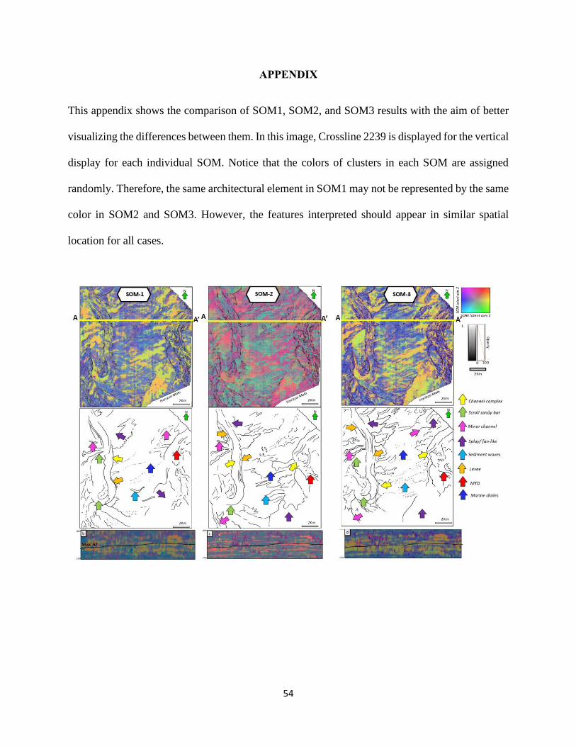
54
APPENDIX
This appendix shows the comparison of SOM1, SOM2, and SOM3 results with the aim of better
visualizing the differences between them. In this image, Crossline 2239 is displayed for the vertical
display for each individual SOM. Notice that the colors of clusters in each SOM are assigned
randomly. Therefore, the same architectural element in SOM1 may not be represented by the same
color in SOM2 and SOM3. However, the features interpreted should appear in similar spatial
location for all cases.
55
CHAPTER 3. USER VS MACHINE SEISMIC ATTRIBUTE SELECTION FOR
UNSUPERVISED MACHINE LEARNING TECHNIQUES: DOES HUMAN INSIGHT
PROVIDE BETTER RESULTS THAN STATISTICALLY CHOSEN ATTRIBUTES?
INTRODUCTION
Conventional seismic interpretation techniques involve seismic attribute calculations and
applications to determine geometries, lithologies, and reservoir properties. In recent years, the use
of machine learning techniques has become a common practice in advanced seismic interpretation
workflows. These methods are based on complex algorithms that allow quick and improved
classification of seismic data than traditional single attribute analysis made by interpreters.
Machine learning (ML) applications within the geosciences extend from predicting seismic
facies, to automatic fault detection. The choice of an unsupervised ML method over a supervised
method depends on the type of data available for the study. In exploration stages, it is often rare to
find well logs or other data. In this scenario, unsupervised methods provide ways to find
relationships among the variables in the data available. However, unsupervised methods require
interpreter evaluation to approve or disapprove the output.
Methods such as Principal Component Analysis (PCA), introduced by Pearson (1901) and
developed by Hotelling (1933), are a common technique to find patterns in data of high dimensions
(Smith, 2002). PCA seeks to reduce a multivariate space (dataset) down to a more manageable size
of relatively independent variables. In seismic interpretation, PCA helps to determine the most
meaningful seismic attributes (Taner, 2001; Roden and Sacrey, 2016). Likewise, SOM is an
unsupervised technique used in multi-attribute analysis to extract additional information from the
seismic response not possible with single attributes (Leal et al., 2019). This method was first coined
by Kohonen (1982), but became popular nowadays due to the increase in computational power.
PCA and SOM have been used for many purposes. For example, in the marketing arena, Das et
56
al., (2016) applied PCA and SOM to find clusters in people's responses regarding the retail store
personality. In seismic data, Coleou et al., (2003) applied SOMs for seismic classification using a
1D latent space. More recently, Guo et al., (2009) computed spectral attributes and applied PCA
to determine the first three principal components of the spectral variation. Later, Matos et al.,
(2007), Roy and Marfurt (2010), and Roy (2013) showed the advantage of extending the SOM
latent space to 2D and 3D, using 2D and 3D colorbars to delineate elements in depositional
environments. More recent studies (Sacrey and Roden, 2014; Roden and Sacrey, 2016; and Leal
et al., 2019) integrated PCA to select attributes, and SOMs to interpret facies in various
depositional environments.
This research investigates the impact of a user-driven (biased) selection of seismic
attributes to perform SOM for seismic facies classification versus a machine- derived selection
(through PCA). We used the Pipeline 3D seismic dataset, in the southern Taranaki basin of New
Zealand, to determine suitable attributes and combinations to interpret deepwater architectural
elements. We explored which attribute selection allows for a reliable and time-efficient
classification to improve interpretation.
MOTIVATION
The motivation of Chapter 3 was to provide a comparison between machine selected
attributes (via principal component analysis) and user-defined attributes (multi-attribute approach
in Chapter 2) (Figure 3-1). To compare methods in a deepwater setting, we evaluated how effective
each combination of attributes was. We explored the advantages and disadvantages of a user-
driven vs. machine conducted attribute selection. We sought to understand the best seismic
attributes to characterize a deepwater setting and compare the generated clusters.
57
PRINCIPAL COMPONENT ANALYSIS (PCA)
PCA is one of the oldest and most known among multivariate analysis techniques
(Jolliffe,1986). It was first introduced by Pearson (1901) and consists of mathematical algorithms
that apply a principal axis method, and transform a set of variables into a smaller number of
variables called principal components (eigenvectors), that still has most of the information present
in the input dataset. Therefore, PCA is primarily used as a dimensionality reduction technique. In
the PCA results, the first principal component (PC1) accounts for as much of the variability in the
data as possible (Figure 3-2), and each succeeding component (PC2, PC3, etc.) accounts for as
much of the remaining variability (Guo et al., 2009; Zhao et al., 2015). Because PCA is based on
Gaussian statistics, the first eigenvalues or PC preserve the most of the signal, and best represent
the variance in the data, while the last PC has uncorrelated noise (Zhao et al., 2015).
In the world of PCA we need to understand two concepts, eigenvalues, and eigenvectors.
Eigenvalues also called characteristic roots, represent the amount of variance/ variation in the total
sample accounted for by factor. If a factor has low eigenvalue, then it contributes little to the
variance. The second concept, eigenvectors, are vectors resulting from the PCA where the first
vector has the highest eigenvalue and represents the maximum variance in the data (Chopra and
Marfurt, 2014).
In geoscience applications, PCA is performed on a square symmetric matrix, usually
covariance matrix (scaled sums of squares and cross products). This mathematical procedure is
applied when the variances of individual variates differ much, or if the units of measurement of
individual variates differ, which is the case for seismic attributes from different types. (Atchley,
2018)
58
PCA has been used as the first step in clustering techniques such as self-organizing maps
(e.g., Leal et al., 2019), generative topographic maps (e.g., Roy, 2013) and support vector machine
analysis (e.g., Zhao et al., 2015), because it reduces the number of attributes for subsequent
analysis (Chopra and Marfurt, 2014). However, one of the drawbacks about PCA is that after the
dimensionality reduction, there is no guarantee that the dimensions or results are interpretable.
METHODOLOGY
For the previous chapter, we performed the dataset inspection and area of interest
definition. For this part of the study, we followed the workflow in Figure 3-3. We used as input a
total of 28 attributes from a variety of textural, geometrical, instantaneous, and spectral attributes.
Table 3-1 presents the attributes considered for input in the PCA. We computed the attributes in
the AASPI software and imported them in Paradise software for the subsequent steps. It is
important to mention that all the seismic volumes should ideally have the same dimensions and be
associated with the same original amplitude volume. The selection of a window of interest allows
for an optimal calculation of preceding methods and avoids miscalculations. Next, we inputted the
28 attributes and ran PCA. We then evaluated the eigenvectors in the section of interest (see AOI
in Chapter 2) and determined the main contributors (attributes).
We considered the most representative attributes (the attributes that contributed the most
to the total variance) in the first three principal components. We then performed SOM to determine
the classes (seismic facies). We selected a neuron configuration of 16, that would represent 16
possible clusters, and 100 epochs (iterations). While the groups themselves are defined in the
original n-dimensional space, they are mapped into a lower-dimensional, typically one- or two-
dimensional, latent space (Wallet et al., 2009). This two dimensional, hexagonal, or rectangular
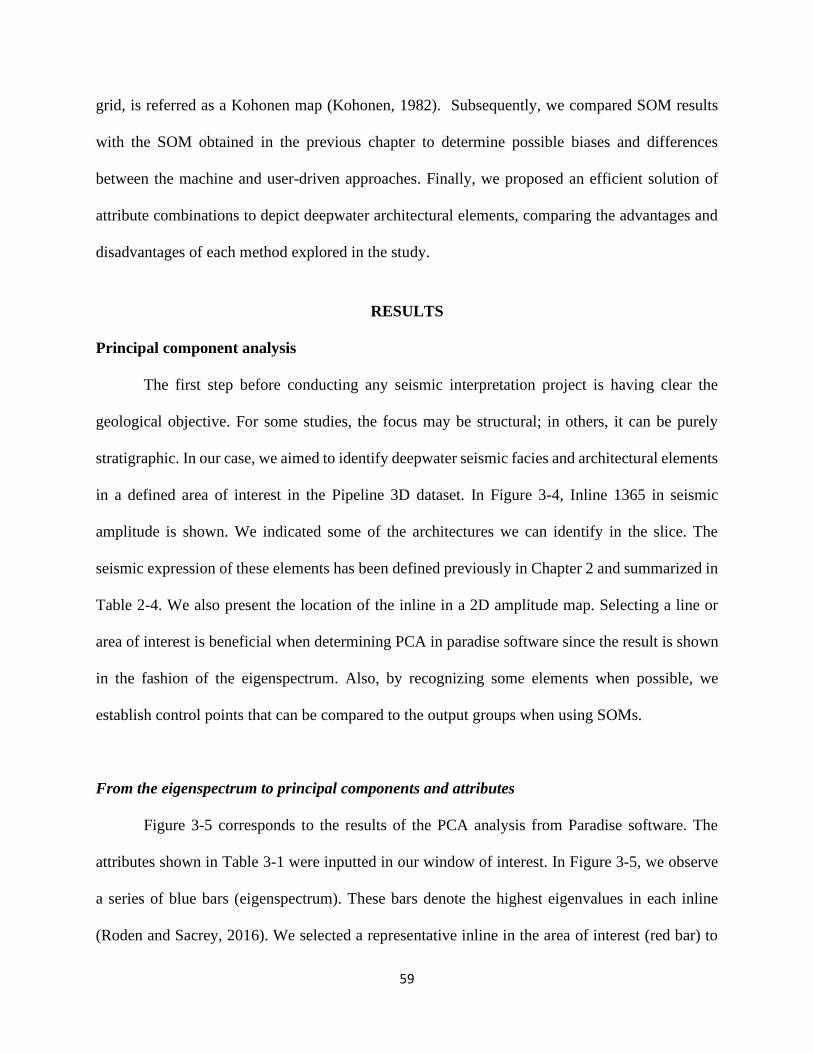
59
grid, is referred as a Kohonen map (Kohonen, 1982). Subsequently, we compared SOM results
with the SOM obtained in the previous chapter to determine possible biases and differences
between the machine and user-driven approaches. Finally, we proposed an efficient solution of
attribute combinations to depict deepwater architectural elements, comparing the advantages and
disadvantages of each method explored in the study.
RESULTS
Principal component analysis
The first step before conducting any seismic interpretation project is having clear the
geological objective. For some studies, the focus may be structural; in others, it can be purely
stratigraphic. In our case, we aimed to identify deepwater seismic facies and architectural elements
in a defined area of interest in the Pipeline 3D dataset. In Figure 3-4, Inline 1365 in seismic
amplitude is shown. We indicated some of the architectures we can identify in the slice. The
seismic expression of these elements has been defined previously in Chapter 2 and summarized in
Table 2-4. We also present the location of the inline in a 2D amplitude map. Selecting a line or
area of interest is beneficial when determining PCA in paradise software since the result is shown
in the fashion of the eigenspectrum. Also, by recognizing some elements when possible, we
establish control points that can be compared to the output groups when using SOMs.
From the eigenspectrum to principal components and attributes
Figure 3-5 corresponds to the results of the PCA analysis from Paradise software. The
attributes shown in Table 3-1 were inputted in our window of interest. In Figure 3-5, we observe
a series of blue bars (eigenspectrum). These bars denote the highest eigenvalues in each inline
(Roden and Sacrey, 2016). We selected a representative inline in the area of interest (red bar) to
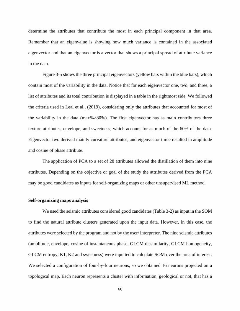
60
determine the attributes that contribute the most in each principal component in that area.
Remember that an eigenvalue is showing how much variance is contained in the associated
eigenvector and that an eigenvector is a vector that shows a principal spread of attribute variance
in the data.
Figure 3-5 shows the three principal eigenvectors (yellow bars within the blue bars), which
contain most of the variability in the data. Notice that for each eigenvector one, two, and three, a
list of attributes and its total contribution is displayed in a table in the rightmost side. We followed
the criteria used in Leal et al., (2019), considering only the attributes that accounted for most of
the variability in the data (max%>80%). The first eigenvector has as main contributors three
texture attributes, envelope, and sweetness, which account for as much of the 60% of the data.
Eigenvector two derived mainly curvature attributes, and eigenvector three resulted in amplitude
and cosine of phase attribute.
The application of PCA to a set of 28 attributes allowed the distillation of them into nine
attributes. Depending on the objective or goal of the study the attributes derived from the PCA
may be good candidates as inputs for self-organizing maps or other unsupervised ML method.
Self-organizing maps analysis
We used the seismic attributes considered good candidates (Table 3-2) as input in the SOM
to find the natural attribute clusters generated upon the input data. However, in this case, the
attributes were selected by the program and not by the user/ interpreter. The nine seismic attributes
(amplitude, envelope, cosine of instantaneous phase, GLCM dissimilarity, GLCM homogeneity,
GLCM entropy, K1, K2 and sweetness) were inputted to calculate SOM over the area of interest.
We selected a configuration of four-by-four neurons, so we obtained 16 neurons projected on a
topological map. Each neuron represents a cluster with information, geological or not, that has a
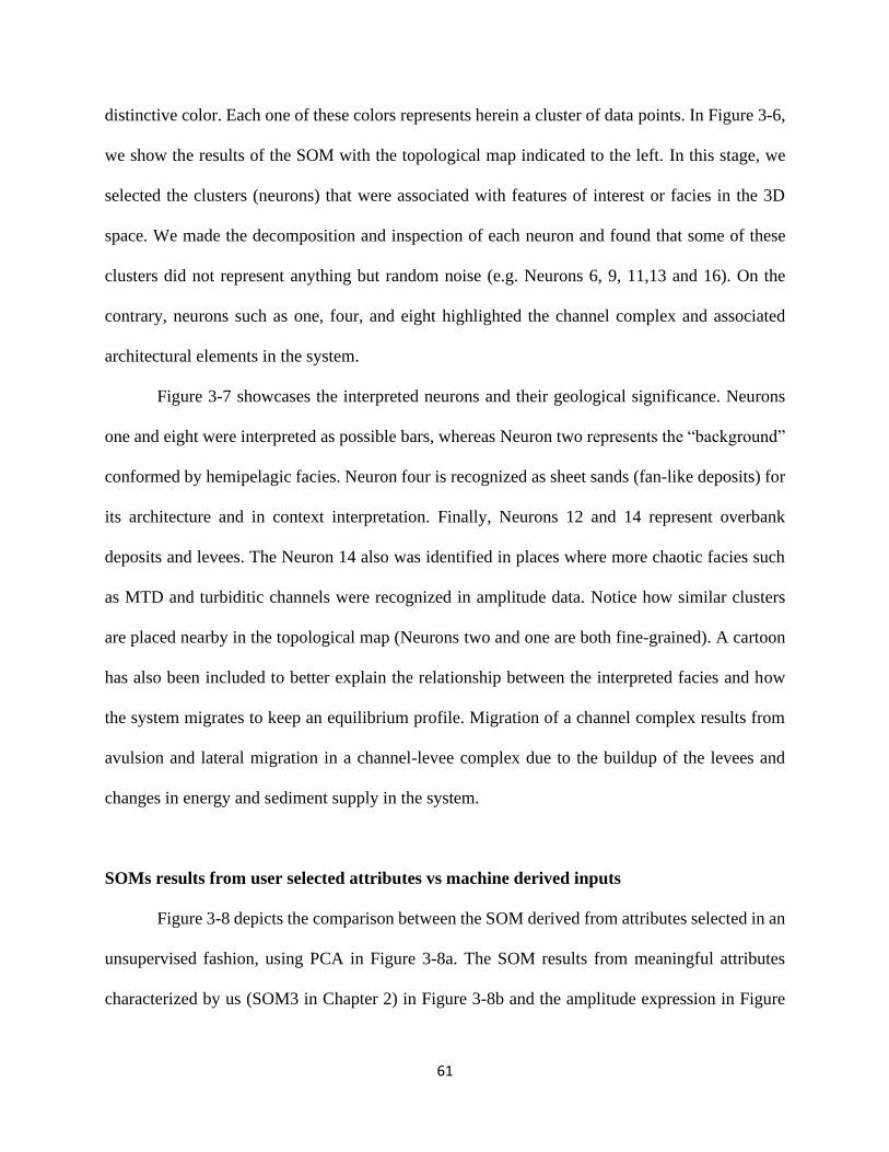
61
distinctive color. Each one of these colors represents herein a cluster of data points. In Figure 3-6,
we show the results of the SOM with the topological map indicated to the left. In this stage, we
selected the clusters (neurons) that were associated with features of interest or facies in the 3D
space. We made the decomposition and inspection of each neuron and found that some of these
clusters did not represent anything but random noise (e.g. Neurons 6, 9, 11,13 and 16). On the
contrary, neurons such as one, four, and eight highlighted the channel complex and associated
architectural elements in the system.
Figure 3-7 showcases the interpreted neurons and their geological significance. Neurons
one and eight were interpreted as possible bars, whereas Neuron two represents the “background”
conformed by hemipelagic facies. Neuron four is recognized as sheet sands (fan-like deposits) for
its architecture and in context interpretation. Finally, Neurons 12 and 14 represent overbank
deposits and levees. The Neuron 14 also was identified in places where more chaotic facies such
as MTD and turbiditic channels were recognized in amplitude data. Notice how similar clusters
are placed nearby in the topological map (Neurons two and one are both fine-grained). A cartoon
has also been included to better explain the relationship between the interpreted facies and how
the system migrates to keep an equilibrium profile. Migration of a channel complex results from
avulsion and lateral migration in a channel-levee complex due to the buildup of the levees and
changes in energy and sediment supply in the system.
SOMs results from user selected attributes vs machine derived inputs
Figure 3-8 depicts the comparison between the SOM derived from attributes selected in an
unsupervised fashion, using PCA in Figure 3-8a. The SOM results from meaningful attributes
characterized by us (SOM3 in Chapter 2) in Figure 3-8b and the amplitude expression in Figure
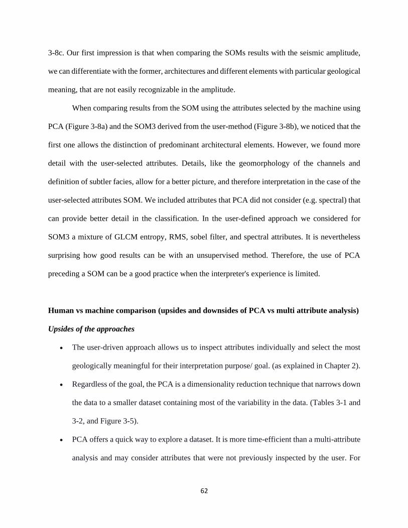
62
3-8c. Our first impression is that when comparing the SOMs results with the seismic amplitude,
we can differentiate with the former, architectures and different elements with particular geological
meaning, that are not easily recognizable in the amplitude.
When comparing results from the SOM using the attributes selected by the machine using
PCA (Figure 3-8a) and the SOM3 derived from the user-method (Figure 3-8b), we noticed that the
first one allows the distinction of predominant architectural elements. However, we found more
detail with the user-selected attributes. Details, like the geomorphology of the channels and
definition of subtler facies, allow for a better picture, and therefore interpretation in the case of the
user-selected attributes SOM. We included attributes that PCA did not consider (e.g. spectral) that
can provide better detail in the classification. In the user-defined approach we considered for
SOM3 a mixture of GLCM entropy, RMS, sobel filter, and spectral attributes. It is nevertheless
surprising how good results can be with an unsupervised method. Therefore, the use of PCA
preceding a SOM can be a good practice when the interpreter's experience is limited.
Human vs machine comparison (upsides and downsides of PCA vs multi attribute analysis)
Upsides of the approaches
• The user-driven approach allows us to inspect attributes individually and select the most
geologically meaningful for their interpretation purpose/ goal. (as explained in Chapter 2).
• Regardless of the goal, the PCA is a dimensionality reduction technique that narrows down
the data to a smaller dataset containing most of the variability in the data. (Tables 3-1 and
3-2, and Figure 3-5).
• PCA offers a quick way to explore a dataset. It is more time-efficient than a multi-attribute
analysis and may consider attributes that were not previously inspected by the user. For
63
instance, envelope attribute (Figure 2-5) is cataloged as good facies discriminator (Chopra
and Marfurt, 2005), but I did not consider it for this 3D volume analysis in Chapter 2).
• The user-selected methods allow integrating different data types that can be tested or
classified to reduce redundancy (e.g. Table 2-5).
• Both methods, implemented an unsupervised machine learning technique (SOM), which
allows to recognize elements that the human may not have been able to identify by himself.
(e.g. Figure 3-8).
Downsides and limitations
• The optimal selection of attributes relies on the interpreter’s experience and understanding
of each attribute significance and it might be biased.
• The PCA results may show attributes that are not the most suitable for the goal (e.g. cosine
of phase, in Figure 2-5), and, also requires data QC, because PCA is sensitive to noise. For
example, Figure 3-6 shows clusters that only contain noise. The PCA will reduce the
amount of data examined, but results may have little to do with physical features of interest
(Lubo-Robles and Marfurt, 2019).
• The multi-attribute approach may result time-consuming if started from zero, but, effective
if combinations used for every setting are documented and followed to apply in similar
geological settings.
• The PCA method suggest attributes that are “main contributors” but that may be similar or
redundant. For example, most positive curvature and maximum curvature (Figure 3-5c).
• Both methods, applied to SOMs, require human inspection and approval in pivotal
moments. The most straight forward example is the validation and interpretation of the
64
SOMs outputs regardless of the initial approach used. Interpreters must apply seismic
geomorphology principles to define the groups of data points with “similar” characteristics
that belong to each cluster.
CONCLUSION
In this chapter we aimed to compare previously user-selected attributes implemented in a
self-organizing map (SOM) technique for deepwater seismic facies interpretation, and attributes
selected statistically by a Principal Component Analysis (PCA). PCA allowed the reduction of a
large dataset of 28 attributes to only nine attributes contained in the principal components. The
first, second, and third principal components contained the most of the variability within the data.
This machine- derived attribute selection included amplitude, cosine of instantaneous phase,
envelope, most positive and most negative curvature, sweetness, and textural attributes such as
GLCM, dissimilarity, entropy and homogeneity to use in the self-organizing maps (SOMs). We
concluded that the machine-based attribute selection is composed of redundant attributes such as
GLCM homogeneity and GLCM entropy, or amplitude and envelope.
We found that the user-driven approach offers a better picture and geological significance
to the interpreter than the machine-driven approach (PCA). The user-driven method helped to
better illustrate the architecture and geomorphology of the elements, and define subtle differences
within them. We suggest a list of attributes provided to use in unsupervised machine learning
methods in similar geological settings (see Chapter 2). However, if the geological setting and
objective differs of the one in this research, the user should define the most suitable attributes for
their geological goal.
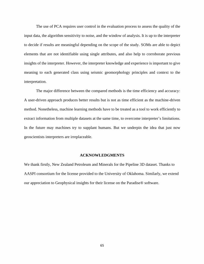
65
The use of PCA requires user control in the evaluation process to assess the quality of the
input data, the algorithm sensitivity to noise, and the window of analysis. It is up to the interpreter
to decide if results are meaningful depending on the scope of the study. SOMs are able to depict
elements that are not identifiable using single attributes, and also help to corroborate previous
insights of the interpreter. However, the interpreter knowledge and experience is important to give
meaning to each generated class using seismic geomorphology principles and context to the
interpretation.
The major difference between the compared methods is the time efficiency and accuracy:
A user-driven approach produces better results but is not as time efficient as the machine-driven
method. Nonetheless, machine learning methods have to be treated as a tool to work efficiently to
extract information from multiple datasets at the same time, to overcome interpreter’s limitations.
In the future may machines try to supplant humans. But we underpin the idea that just now
geoscientists interpreters are irreplaceable.
ACKNOWLEDGMENTS
We thank firstly, New Zealand Petroleum and Minerals for the Pipeline 3D dataset. Thanks to
AASPI consortium for the license provided to the University of Oklahoma. Similarly, we extend
our appreciation to Geophysical insights for their license on the Paradise® software.
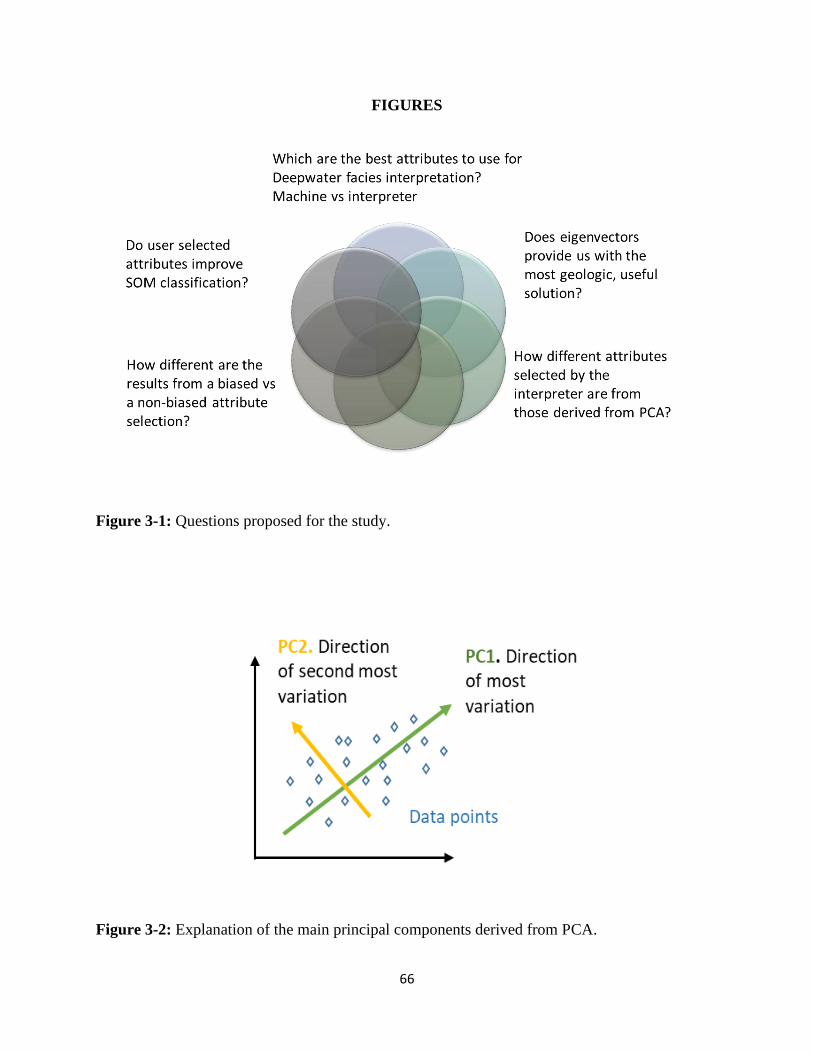
66
FIGURES
Figure 3-1: Questions proposed for the study.
Figure 3-2: Explanation of the main principal components derived from PCA.
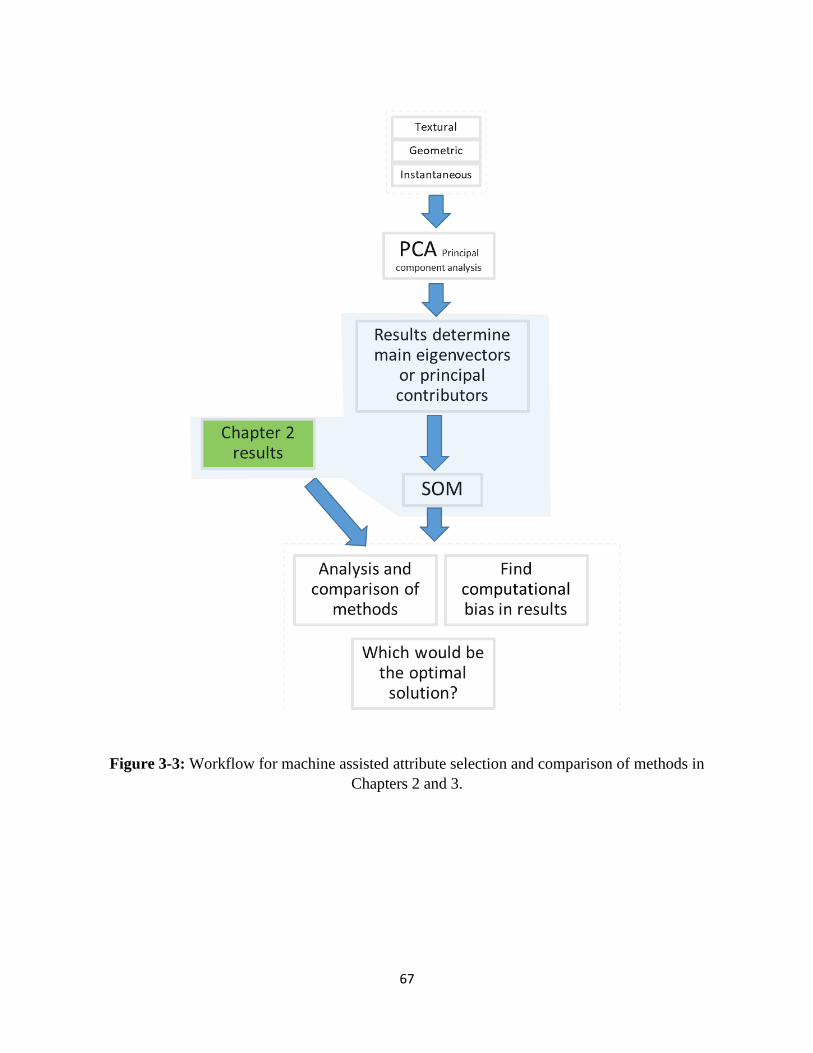
67
Figure 3-3: Workflow for machine assisted attribute selection and comparison of methods in
Chapters 2 and 3.
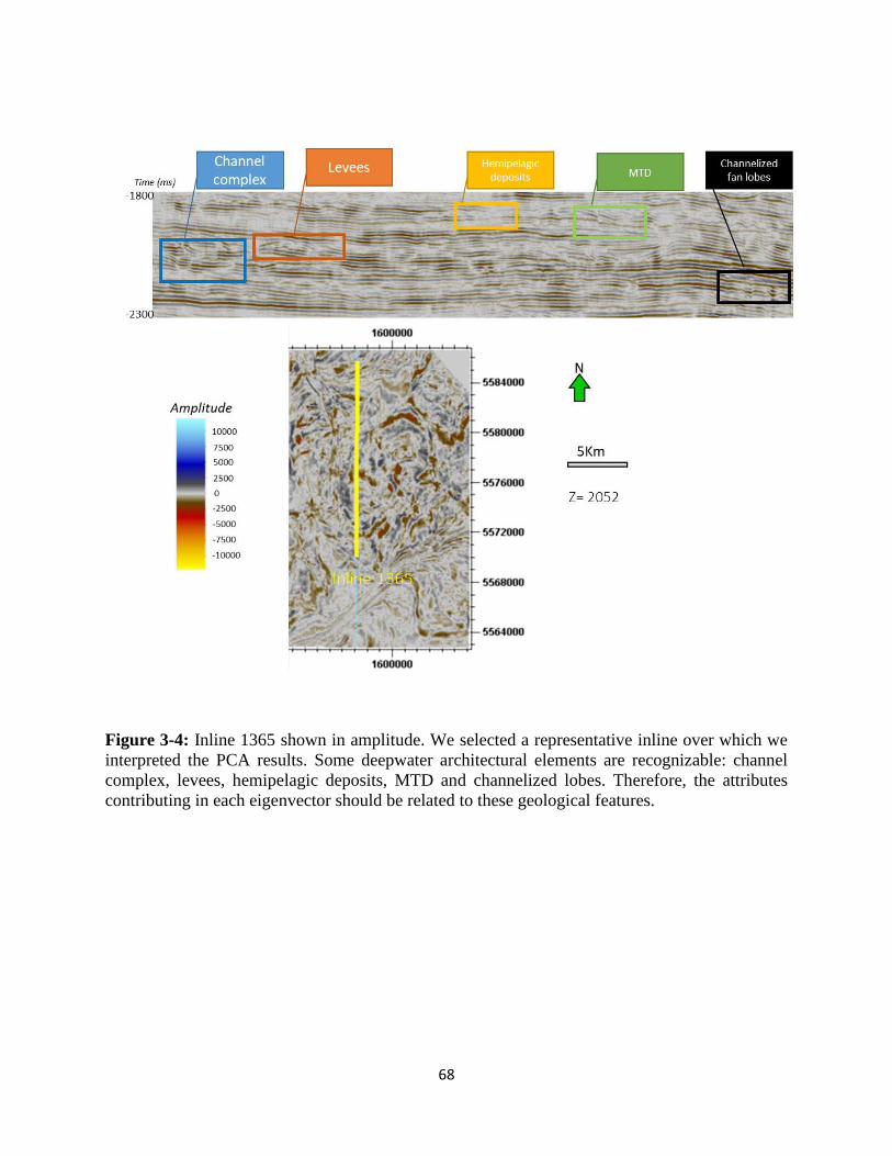
68
Figure 3-4: Inline 1365 shown in amplitude. We selected a representative inline over which we
interpreted the PCA results. Some deepwater architectural elements are recognizable: channel
complex, levees, hemipelagic deposits, MTD and channelized lobes. Therefore, the attributes
contributing in each eigenvector should be related to these geological features.
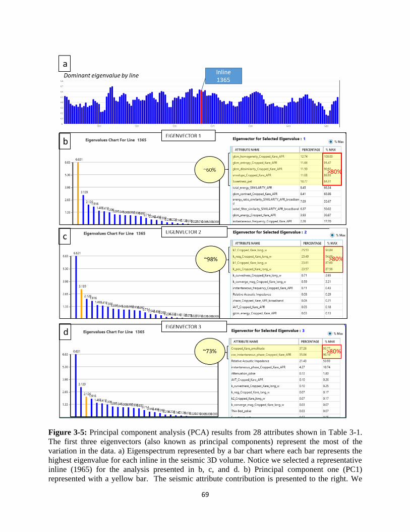
69
Figure 3-5: Principal component analysis (PCA) results from 28 attributes shown in Table 3-1.
The first three eigenvectors (also known as principal components) represent the most of the
variation in the data. a) Eigenspectrum represented by a bar chart where each bar represents the
highest eigenvalue for each inline in the seismic 3D volume. Notice we selected a representative
inline (1965) for the analysis presented in b, c, and d. b) Principal component one (PC1)
represented with a yellow bar. The seismic attribute contribution is presented to the right. We
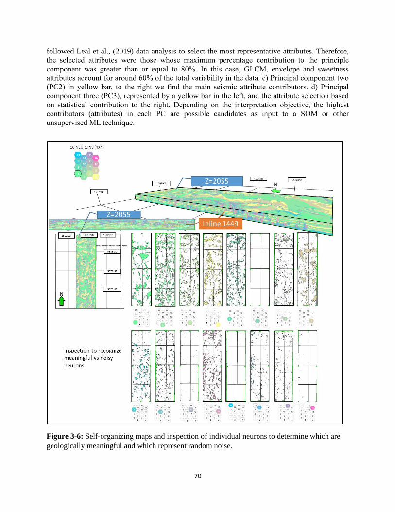
70
followed Leal et al., (2019) data analysis to select the most representative attributes. Therefore,
the selected attributes were those whose maximum percentage contribution to the principle
component was greater than or equal to 80%. In this case, GLCM, envelope and sweetness
attributes account for around 60% of the total variability in the data. c) Principal component two
(PC2) in yellow bar, to the right we find the main seismic attribute contributors. d) Principal
component three (PC3), represented by a yellow bar in the left, and the attribute selection based
on statistical contribution to the right. Depending on the interpretation objective, the highest
contributors (attributes) in each PC are possible candidates as input to a SOM or other
unsupervised ML technique.
Figure 3-6: Self-organizing maps and inspection of individual neurons to determine which are
geologically meaningful and which represent random noise.
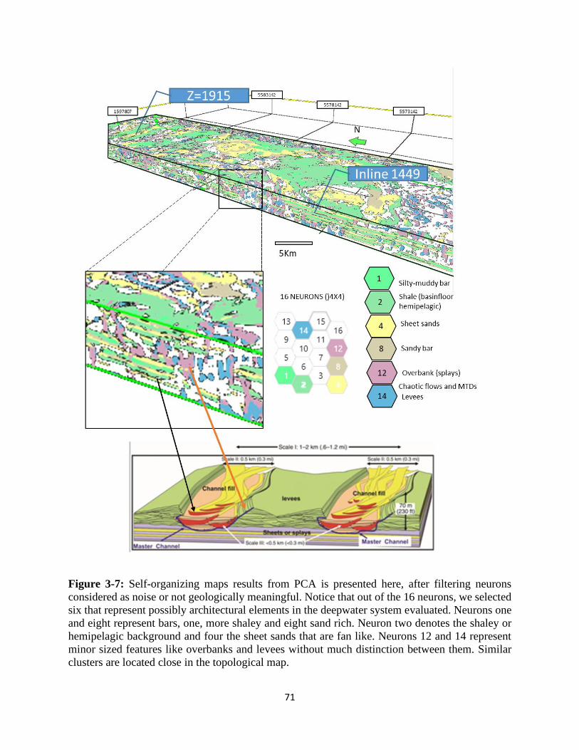
71
Figure 3-7: Self-organizing maps results from PCA is presented here, after filtering neurons
considered as noise or not geologically meaningful. Notice that out of the 16 neurons, we selected
six that represent possibly architectural elements in the deepwater system evaluated. Neurons one
and eight represent bars, one, more shaley and eight sand rich. Neuron two denotes the shaley or
hemipelagic background and four the sheet sands that are fan like. Neurons 12 and 14 represent
minor sized features like overbanks and levees without much distinction between them. Similar
clusters are located close in the topological map.
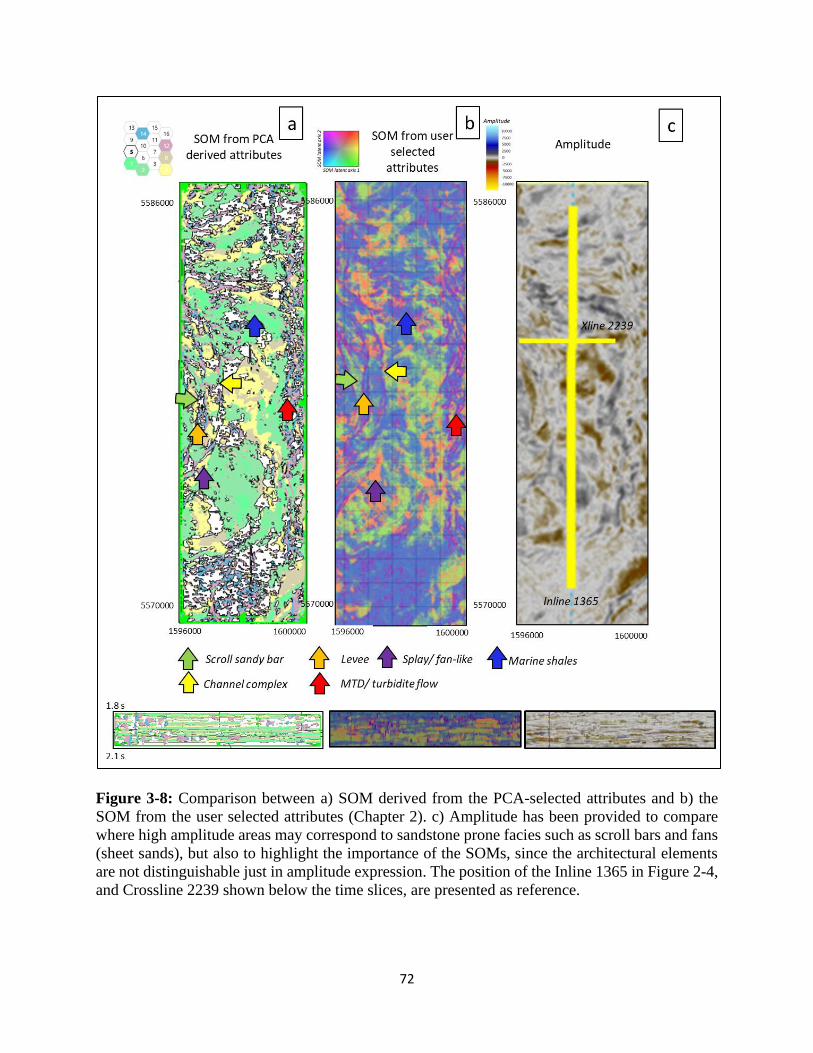
72
Figure 3-8: Comparison between a) SOM derived from the PCA-selected attributes and b) the
SOM from the user selected attributes (Chapter 2). c) Amplitude has been provided to compare
where high amplitude areas may correspond to sandstone prone facies such as scroll bars and fans
(sheet sands), but also to highlight the importance of the SOMs, since the architectural elements
are not distinguishable just in amplitude expression. The position of the Inline 1365 in Figure 2-4,
and Crossline 2239 shown below the time slices, are presented as reference.
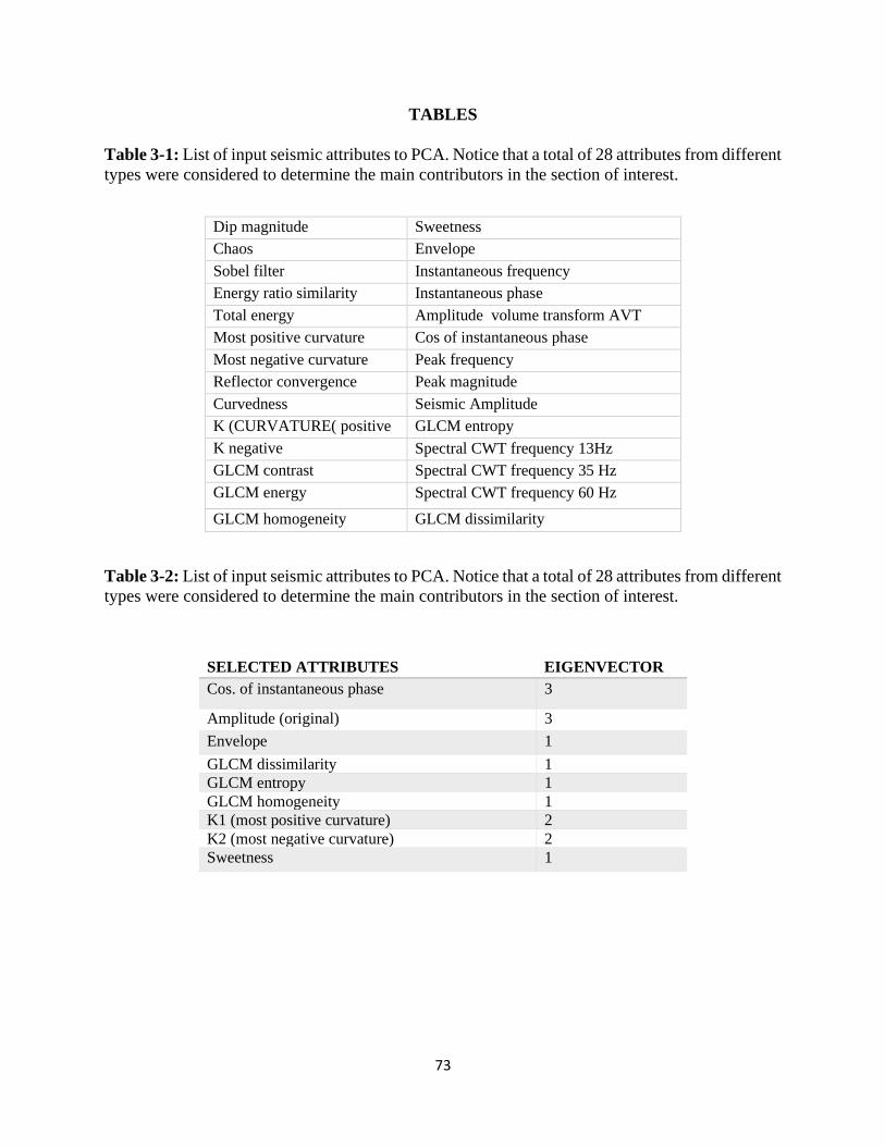
73
TABLES
Table 3-1: List of input seismic attributes to PCA. Notice that a total of 28 attributes from different
types were considered to determine the main contributors in the section of interest.
Dip magnitude Sweetness
Chaos Envelope
Sobel filter Instantaneous frequency
Energy ratio similarity Instantaneous phase
Total energy Amplitude volume transform AVT
Most positive curvature Cos of instantaneous phase
Most negative curvature Peak frequency
Reflector convergence Peak magnitude
Curvedness Seismic Amplitude
K (CURVATURE( positive GLCM entropy
K negative Spectral CWT frequency 13Hz
GLCM contrast Spectral CWT frequency 35 Hz
GLCM energy Spectral CWT frequency 60 Hz
GLCM homogeneity GLCM dissimilarity
Table 3-2: List of input seismic attributes to PCA. Notice that a total of 28 attributes from different
types were considered to determine the main contributors in the section of interest.
SELECTED ATTRIBUTES EIGENVECTOR
Cos. of instantaneous phase 3
Amplitude (original) 3
Envelope 1
GLCM dissimilarity 1
GLCM entropy 1
GLCM homogeneity 1
K1 (most positive curvature) 2
K2 (most negative curvature) 2
Sweetness 1
74
REFERENCES
Atchley, W.R, 2007, Introduction to Principal Components and Factor Analysis. Retrieved from
ftp://statgen.ncsu.edu/pub/thorne/molevoclass/AtchleyOct19.pdf.
Chopra, S; and K. J. Marfurt, 2005, Seismic attributes- A historical perspective: Interpretation,
70, 5, IS0-Z82.
Chopra, S; and K. J. Marfurt, 2014, Churning seismic attributes with principal component analysis:
86th annual international meeting, SEG, Expanded abstracts 2672-2676.
Coleou, T., M. Poupon., and K. Azbel, 2003, Unsupervised seismic facies classification: A review
and comparison of techniques and implementation: The Leading Edge, 22, 942–953.
Das, G., m. Chattopadhyay., S. Gupta, 2016, A comparison of self-organising maps and principal
component analysis. International Journal of Market research 58, no 6.815-834. DOI:
10.2501/IJMR-2016-000
Guo, H., K. J. Marfurt, and J. Liu, 2009, Principal component spectral analysis: Geophysics, 74,
no. 4, 35–43, doi: 10.1190/1.3119264.
Hotelling, H, 1933. Analysis of a Complex of Statistical Variables into Principal Components.
Journal of Educational Psychology, 24(6 and 7), 417–441 and 498–520.
Jolliffe.I.T, 1986, Principal component analysis. Springer. ISBN 978-1-4757-1906-2 ISBN 978-
1-4757-1904-8 (eBook) DOI 10.1007/978-1-4757-1904-8
Kohonen, T, 1982, Self-organized formation of topologically correct feature maps: Biological
cybernetics, 43, 59-69.
La Marca-Molina, K., C. Silver., H.Bedle., and R. Slatt, 2019. Seismic facies identification in a
deepwater channel complex applying seismic attributes and unsupervised machine learning
techniques. A case study in the Taranaki Basin, New Zealand: 89th annual international
meeting, SEG, Expanded abstracts, 2059-2063.
Leal. J., R. Jeronimo., F. Rada., R. Viloria., and R. Roden, 2019, Net reservoir discrimination
through multi-attribute analysis. First Break, .37, 9. P. 77-86.
Lubo-Robles, D., K. Marfurt, 2019, Unsupervised seismic facies classification using ICA:
Interpretation, 7, 3, Society of Exploration Geophysicists.
Matos, M. C., P. L. Osorio, and P. Johann, 2007, Unsupervised seismic facies analysis using
wavelet transform and self-organizing maps: Geophysics, 72, p. P9- P21
75
Pearson. K, 1901, On Lines and Planes of Closest Fit to Systems of Points in Space. Philosophical
Magazine, 6, 2(11), 559–572.
Roden, R., and Sacrey, D, 2016. Seismic interpretation with machine learning: GeoExpro. 13, 6.
pp 50-53 https://www.geoexpro.com/articles/2017/01/seismic-interpretation-with-
machine-learning
Roy, A., and K. J. Marfurt, 2010, Applying self-organizing maps of multiattributes, an example
from the Red-Fork Formation, Anadarko Basin: 81st Annual International Meeting Society
of Exploration Geophysicists, Expanded Abstracts, p. 1591-1595.
Roy, A, 2013, Latent space classification of seismic facies: Ph.D. dissertation, University of
Oklahoma.
Sacrey, D., and R. Roden., 2014, Understanding attributes and their use in the application of neural
analysis- case histories both conventional and unconventional: Search and discovery article
#41473.
Silver, C., K. La Marca-Molina., and H. Bedle, 2019, Seismic geomorphology of deep-water
channel systems in the southern Taranaki Basin: 89th annual meeting, SEG, Expanded
Abstracts (pp. 2018-2022). Society of Exploration Geophysicists.
Smith. L, 2002, A tutorial on principal component analysis. Statistics ISBN: 0471852236
Taner. M, 2001, Seismic attributes: RECORDER. 26, 07. Canadian Society of Exploration
Geophysicists.
Wallet, B. C., M.C.de Matos., J.T. Kwiatkowski., and Y. Suarez, 2009, Latent space modeling of
seismic data: An overview: The Leading Edge, 28(12), 1454-1459.
Zhao, T; V. Jayaram., A. Roy., and K. Marfurt, 2015, A comparison of classification techniques
for seismic facies recognition: Interpretation. 3, no. 4, SAE29-SAE58.