University of Texas, MD Anderson Cancer Center

University of Texas, MD Anderson CancerCenter

UT MD Anderson Cancer Center Department of BiostatisticsWorking Paper Series

Year Paper

Bayesian Hypothesis Tests UsingNonparametric Statistics

Ying Yuan∗ Valen E. Johnson†

∗M. D. Anderson Cancer Center, [email protected]†M.D. Anderson Cancer Center

This working paper is hosted by The Berkeley Electronic Press (bepress) and may not be commer-cially reproduced without the permission of the copyright holder.

http://biostats.bepress.com/mdandersonbiostat/paper21

Copyright c©2006 by the authors.

Bayesian Hypothesis Tests UsingNonparametric Statistics

Ying Yuan and Valen E. Johnson

Abstract

Traditionally, the application of Bayesian testing procedures to classical nonpara-metric settings has been restricted by difficulties associated with prior specifica-tion, prohibitively expensive computation, and the absence of sampling densitiesfor data. To overcome these difficulties, we model the sampling distributionsof nonparametric test statistics—rather than the sampling distributions of origi-nal data—to obtain the Bayes factors required for Bayesian hypothesis tests. Weapply this methodology to construct Bayes factors from a wide class of nonpara-metric test statistics having limiting normal or chi-square distributions. We alsodemonstrate how this testing strategy can be extended to simplify meta-analysesin which only p values or the values of test statistics have been reported.

Bayesian Hypothesis Tests Using Nonparametric Statistics

Ying Yuan and Valen E. Johnson

Department of Biostatistics and Applied Mathmetics, M.D. Anderson Cancer Center,

Houston, TX, U.S.A.

[email protected] [email protected]

Summary

Traditionally, the application of Bayesian testing procedures to classical nonparametric set-

tings has been restricted by difficulties associated with prior specification, prohibitively ex-

pensive computation, and the absence of sampling densities for data. To overcome these

difficulties, we model the sampling distributions of nonparametric test statistics—rather

than the sampling distributions of original data—to obtain the Bayes factors required for

Bayesian hypothesis tests. We apply this methodology to construct Bayes factors from a

wide class of nonparametric test statistics having limiting normal or χ2 distributions. We

also demonstrate how this testing strategy can be extended to simplify meta-analyses in

which only p values or the values of test statistics have been reported.

Key words: Bayes factor, nonparametric hypothesis test, sign test, Wilcoxon signed rank

test, Mann-Whitney-Wilcoxon test, Kruskal-Wallis test, log-rank test

1

Hosted by The Berkeley Electronic Press

1 Introduction

In parametric settings, the use of Bayesian methodology for conducting hypothesis tests has

been limited by two factors. First, Bayesian test procedures require the specification of in-

formative prior densities on parameters appearing in the parametric statistical models that

comprise each hypothesis. Second, even when it is possible to subjectively define these prior

densities (or to define “objective” substitutes for them), the calculation of Bayes factors

often involves the evaluation of high-dimensional integrals. This can be a prohibitively ex-

pensive undertaking for non-statisticians, both from a numerical and conceptual perspective.

Together, these two factors have severely limited the application of Bayesian methodology

to testing problems.

In nonparametric hypotheses testing, a third difficulty arises. Namely, sampling dis-

tributions for data are not specified. Without sampling distributions for data, Bayesian

hypothesis tests cannot be performed.

The goal of this article is to overcome all three of these impediments to the application

of Bayesian testing procedures by using nonparametric test statistics to define Bayes factors,

which represent the factors that multiply the prior odds assigned to the null and alternative

hypotheses to obtain the posterior odds. Our approach eliminates the second and third

obstacles to calculating these factors, and substantially diminishes the first. Our approach

is based on an extension of methodology described in Johnson (2005).

Given the broad application of nonparametric test statistics and the ready availability of

software to perform classical significance tests based on these statistics, a few preliminary

2


comments regarding our motivation for “mixing paradigms” are perhaps warranted.

From a Bayesian perspective, the use of the p value as a measure of evidence in hypothesis

testing can been criticized from several perspectives (Berger and Delampady, 1987; Berger

and Sellke, 1987; Goodman, 1999a, 1999b, 2001). One important criticism of p values is that

they tend to systematically reject the null hypothesis in large samples—the so called Lindley

paradox (1957). This problem is particularly pronounced in, for example, sample surveys or

large clinical trials in which thousands of observations are collected. In such settings, the

null hypothesis is seldom exactly correct and so is rejected. Bayesian testing methods do

not suffer from the same deficiency: If alternative models that differ from the null model

in substantively meaningful ways are specified, then the null hypothesis is not necessarily

rejected as sample sizes become large.

As proposed by Fisher (1956), the p value represents an informal measure of discrepancy

between the data and the null hypothesis. However, it is important to remember that the p

value does not provide a formal mechanism for assessing the evidence contained in data from

a single experiment. Although the p value is often confused with the Neyman-Pearson Type

1 error rate, which has a valid frequentist interpretation, the data-dependent p value does

not. Berger and Delampady (1987) and Goodman (1999a) provide more detailed discussion

of this issue.

Even if p values did represent approximate long-run error rates, they would still fail to

answer the question of interest in most testing problems: In light of observed data from the

current experiment and existing scientific knowledge, is there enough evidence to reject the

null hypothesis? Unfortunately, the p value does not have a direct relation to the probability

3


of observing data under either the null or alternative hypotheses. Instead, it represents

only the null probability of observing data as extreme or more extreme than was actually

observed. As Jeffreys (1961) pointed out, this means that “a hypothesis that may be true

may be rejected because it has not predicted observable results that have not occurred.”

P values also lack a quantitative interpretation in terms of the amount of evidence against

the null hypothesis. For example, p values of both 0.01 and 0.001 result in the rejection of the

null hypothesis in a 5% Neyman-Pearson test, but there is no mechanism to compare these

values quantitatively. That is, a p value of 0.001 does not present 10 times more evidence

against the null hypothesis than does a p value of 0.01. In contrast, Bayes factors and

posterior model probabilities naturally lend themselves to such quantitative comparisons.

Another objection to p values is their tendency to overstate evidence against the null

hypothesis, especially when testing point null hypotheses (e.g., Dickey, 1977; Berger and

Sellke, 1987). Berger and Sellke (1987) show that the actual evidence against a null hypoth-

esis (as measured by its posterior probability) can differ by an order of magnitude from the

p value. When testing a normal mean, for instance, if both hypotheses are deemed equally

likely before seeing the result of an experiment, data that yield a p value of 0.05 result in

a posterior probability of the null hypothesis of at least 0.3 for a broad class of objective

alternative hypotheses. In certain cases, like one-sided hypothesis testing, the p value and

Bayesian posterior probability of null hypothesis may be reconcilable (Casella and Berger,

1987), but even then their interpretations are quite different.

Finally, it is difficult to combine the evidence from different experiments using p values.

Standard meta-analyses weight experiments by their resulting precisions and calculate the

4


p value based on the combined dataset. Unfortunately, this p value has little relation to

the p values obtained from the individual experiments. In contrast, Bayes factors provide a

natural and intuitive way to combine evidence from different experiments.

Our motivation for defining Bayes factors based on non-parametric test statistics is to

avoid many of the pitfalls inherent to p values. As we demonstrate in the sequel, our method-

ology allows us to transform test statistics to an appropriate—and interpretable—probability

scale, rather than to what is essentially an uncalibrated and comparatively uninterpretable

p-value scale.

The role of Bayes factors in parametric hypothesis testing has been studied in great depth.

Kass and Raftery (1995) provide a recent review. In contrast, comparatively little research

has been reported for computing Bayes factor in the nonparametric hypotheses testing, at

least in the classical sense of nonparametric statistics (see Rousseau (2006) for a discussion of

methodology for defining and calculating Bayes factors for Bayesian nonparametric models).

Our approach is based on the observation that, although the sampling density f(x|θ) of

the data X is not specified in nonparametric tests, the distribution of the test statistic, say

T (X), is often known under both null and alternative hypotheses, at least asymptotically.

To make this notion more precise, we assume for the remainder of this article that the

sampling density of the test statistic T (X) can be expressed as g(T (x)|θ), where g denotes

a probability density function defined with respect to an appropriate underlying measure,

and θ may be either a scalar or vector-value parameter. Under the null hypothesis H0, we

assume that θ = θ0 for a known value θ0. Under the alternative hypothesis H1, we assume

that the sampling distribution of T is obtained by averaging over a prior density π(θ) defined

5


on the domain of θ. When these assumptions hold, the Bayes factor based on t = T (X) can

be defined as

BF01(t) =g(t|θ0)∫

g(t)|θ)π(θ) dθ. (1)

For suitable choices of π(θ), we find that Bayes factors based on nonparametric test statistics

can often be expressed in simple form. As a result, it is possible to obtain lower bounds on

the posterior probability of the null hypothesis by maximizing over the marginal likelihood

of the test statistic under H1. Taking this approach eliminates much of the subjectivity

normally associated with the definition of Bayes factors.

2 Methods

Many nonparametric test statistics have limiting distributions that are either normal or χ2.

While our methods can (in some cases) be applied in finite sample settings when suitable

distributions for test statistics under the alternative model can be defined, it is generally

more straightforward to specify alternative distributions in the large sample setting. For this

reason, we restrict attention to this case and begin with nonparametric statistics that have

limiting normal distributions.

2.1 Bayes factor for nonparametric test statistics having limiting

normal distribution

The asymptotic normality of a variety of nonparametric test statistics has been established by

the theory of U -statistics (Hoeffding, 1948) and linear rank statistics (Hajek, 1961; Chernoff

6


and Savage, 1985). These results are widely used in practice to approximate exact sampling

distributions of nonparametric test statistics which usually do not have closed forms and

have to be computed numerically.

The class of nonparametric test statistics with limiting normal distributions includes a

large number of commonly used nonparametric statistics. Among these are the sign test and

Wilcoxon signed rank test for one-sample location problems, the Mann-Whitney-Wilcoxon

test for two-sample location problems, the Ansari-Bradley test and Mood test for scale

problems, the Randall’s tau and Spearman test for testing independence, the Theil test for

slope parameters in regression problems, the Mantel test (or logrank test), and the Hollander-

Proschan test of exponentiality in survival analysis.

In order to describe how statistics from these tests can be used to define Bayes factors, let

Tk, k = 1, 2 . . ., denote a sequence of nonparametric test statistics based on nk observations,

and suppose that nk → ∞ as k → ∞. Consider the test of the null hypothesis

H0 : θ = θ0

versus the local (or contiguous) alternative

H1(nk) : θk = θ0 + ∆/√

nk.

This form of the alternative hypothesis is often called the Pitman translation alternative

(e.g., Randles and Wolfe 1979).

Our attention focuses on the asymptotic distribution of the standardized value of Tk,

T ∗k =

Tk − µk(θ0)

σk(θ0),

7


where µk and σk are the mean and standard deviation of Tk, respectively. Under H0, we

assume that T ∗k has a limiting standard normal distribution. Under H1(nk), the asymptotic

distribution of T ∗k is given in the following Lemma. The proof appears in the Appendix.

Lemma 1. Assume H1(nk) and conditions A1–4 below apply.

(A1) Tk−µk(θk)σk(θk)

L−→ N(0, 1),

(A2) σk(θk)/σk(θ0)p−→ 1,

(A3) µk(θ) is differentiable at θ0,

(A4)µ′

k(θ0)

√nkσk(θ0)

p−→ C where C is a constant.

Then T ∗k

L−→ N(C∆, 1).

We note that each of the nonparametric statistics mentioned above satisfy these as-

sumptions, and that similar conditions are often required in evaluating Pitman’s asymptotic

relative efficiency (Noether 1955). The value of C is the efficacy of the test based on Tk.

With the asymptotic distribution of T ∗k under both H0 and H1 known, the following result

follows from Bayes theorem.

Theorem 1. If assumptions A1–4 of Lemma 1 are satisfied, and the scalar parameter ∆ is

assumed a priori to follow a N(0, τ 2) distribution, then the Bayes factor based on T ∗k is given

by

BF01(T∗) = (1 + C2τ 2)1/2exp

{− C2τ 2T ∗

k2

2(1 + C2τ 2)

}. (2)

The prior density assumed for ∆ in the above theorem centers the distribution of θ on

the null value of θ = θ0. Such centering is natural under classes of local alternatives and also

is consistent with the general philosophy advocated by Jeffreys (1961).

8


There is an interesting parallel between the result of Theorem 1 and results cited in

Johnson (2005) for χ2 statistics. Under the conditions of the theorem, the random variable

T ∗k

2 has a limiting χ2 distribution with 1 degree freedom under H0, and a limiting noncentral

χ2 distribution with 1 degree freedom and non-centrality parameter C2∆2 under H1(nk).

If ∆ ∼ N(0, τ 2) a priori, then the marginal distribution of T ∗k

2 under H1(nk) is a gamma

distribution with shape parameter 1/2 and scale parameter 1/[2(C2τ+1)]. Letting Ga(·|α, β)

denote a gamma density with shape parameter α and scale parameter β, the Bayes factor

based on T ∗k

2 is given by

BF01(T∗k

2) =Ga(T ∗

k2|1

2, 1

2)

Ga(T ∗k

2|12, 1

2(C2τ2+1))

= (1 + C2τ 2)1/2 exp

{− C2τ 2T ∗

k2

2(1 + C2τ 2)

}

= BF01(T∗k )

This equation provides a connection to results presented for χ2 statistics in Johnson (2005)

and is explored further in Section 2.2.

Several approaches might be taken for setting the value of the parameter τ that appears

in (2) . If possible, prior information or scientific guidance should be used to subjectively

specify an appropriate prior distribution on τ . In the absence of such information, τ can be

(objectively) determined by equating its value to its maximum marginal likelihood estimate

(MMLE) under the alternative hypothesis. This leads to an upper bound on the Bayes factors

against point null hypotheses. This strategy has previously been advocated by Edwards,

Lindman and Savage (1963), Dickey (1977), Good (1950, 1958, 1967, 1986), Berger (1985),

Berger and Sellke (1987), and Berger and Delampday (1987), among others.

9


Under the conditions of Theorem 1, the MMLE of τ 2 under H1(n) is given by

τ 2 =T ∗

k2 − 1

C2

provided that the statistic T ∗k

2 exceeds its expectation under H0 (i.e. T ∗k

2 > 1). The Bayes

factor obtained by setting τ to this value is

B̃F 01(T∗) = |T ∗

k |exp

(1 − T ∗

k2

2

).

This value represents an upper bound on the weight of evidence against H0. Note that

B̃F 01(T∗) does not depend on the constant C, which is fortunate since C often depends on

the unknown null distribution of the data. When T ∗k

2 < 1, the alternative model collapses

onto the null model (τ = 0), making the Bayes factor equal to 1. For T ∗k

2 > 1, if equal

probabilities are assigned to H0 and H1 a priori, the corresponding lower bound on the

posterior probability of H0 is

P̃ (H0|x) =

(1 +

1

|T ∗k |

eT∗

k2−1

2

)−1

. (3)

From a philosophical perspective, it is interesting to compare probability (3) with the p

value based on the large sample normal approximation. Given the value of test statistics

T ∗k (x), the p value under the normal approximation is 2(1−Φ(T ∗

k )), where Φ(·) denotes the

standard normal distribution function. The following theorem shows that this p value is

substantially smaller than the posterior probability of the null hypothesis for this class of

tests. The proof of this theorem follows along lines similar to those exposed in Berger and

Sellke (1987).

10


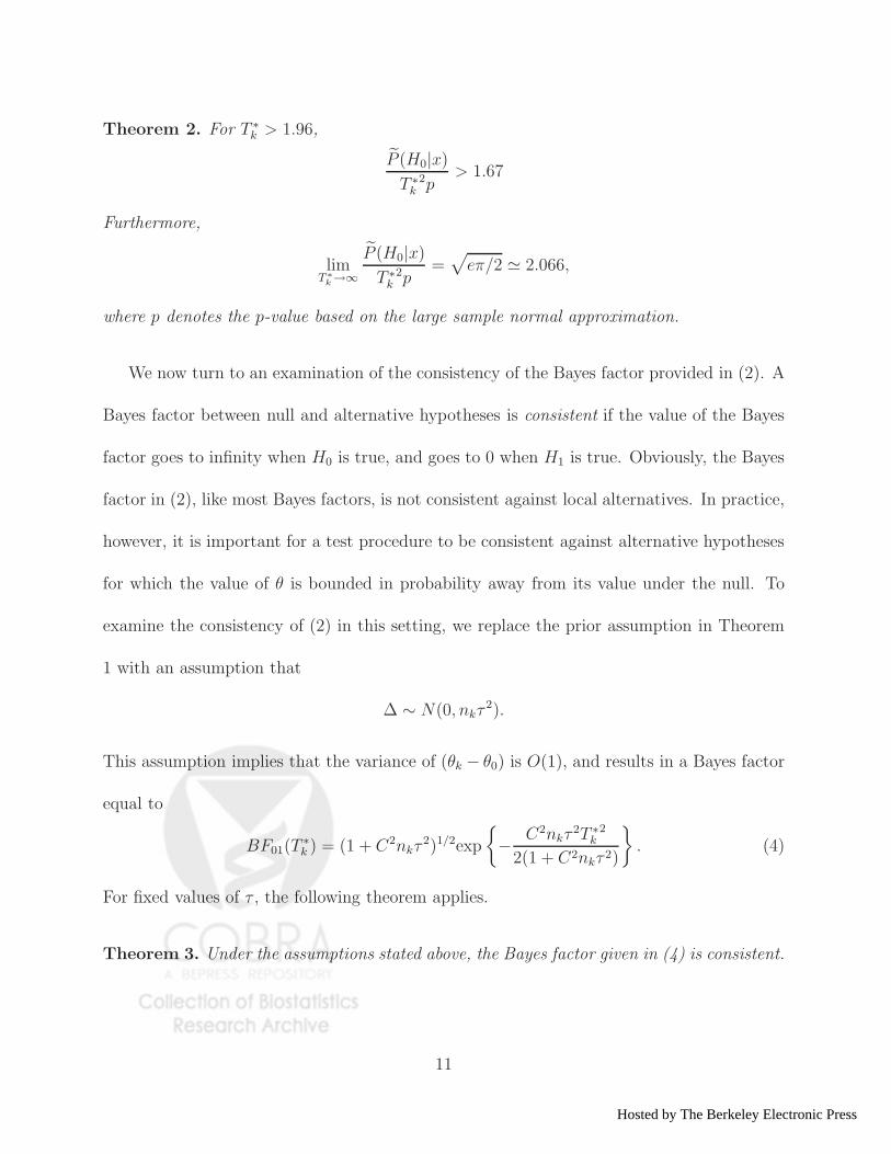
Theorem 2. For T ∗k > 1.96,

P̃ (H0|x)

T ∗k

2p> 1.67

Furthermore,

limT ∗

k→∞

P̃ (H0|x)

T ∗k

2p=

√eπ/2 ≃ 2.066,

where p denotes the p-value based on the large sample normal approximation.

We now turn to an examination of the consistency of the Bayes factor provided in (2). A

Bayes factor between null and alternative hypotheses is consistent if the value of the Bayes

factor goes to infinity when H0 is true, and goes to 0 when H1 is true. Obviously, the Bayes

factor in (2), like most Bayes factors, is not consistent against local alternatives. In practice,

however, it is important for a test procedure to be consistent against alternative hypotheses

for which the value of θ is bounded in probability away from its value under the null. To

examine the consistency of (2) in this setting, we replace the prior assumption in Theorem

1 with an assumption that

∆ ∼ N(0, nkτ2).

This assumption implies that the variance of (θk − θ0) is O(1), and results in a Bayes factor

equal to

BF01(T∗k ) = (1 + C2nkτ

2)1/2exp

{− C2nkτ

2T ∗k

2

2(1 + C2nkτ 2)

}. (4)

For fixed values of τ , the following theorem applies.

Theorem 3. Under the assumptions stated above, the Bayes factor given in (4) is consistent.

11


2.1.1 Application to Specific Nonparametric Tests

Wilcoxon signed rank test and sign test

Consider paired replicate data for n subjects, and suppose that (Xi, Yi), i = 1, . . . , n, denote

pre- and post-treatment measurements for n items or subjects. Define Zi = Yi − Xi to be

the associated treatment effects, and suppose the treatment effects are independent and dis-

tributed according to an unknown distribution function F (Z|θ). Assume further that F (Z|θ)

is symmetric around θ and that we wish to test the null hypothesis of no treatment effect

against a two-sided alternative using the Wilcoxon signed rank test. Under an appropriate

parameterization, we assume that the null hypothesis may be expressed H0 : θ = 0, while

the alternative hypothesis may be represented H1 : θ 6= 0.

To define the Wilcoxon signed rank test statistic, order the absolute values |Z1|, . . . , |Zn|

from smallest to largest. Let Ri denote the rank of |Zi| and define the indicator variable

δi, i = 1, . . . , n, as

δi =

1 if Zi > 0

0 if Zi < 0

.

The Wilcoxon signed rank statistics W is then given by

W =n∑

i=1

δiRi.

The limiting distribution of W , suitably standardized, is a normal distribution under H0:

W ∗ =W − E(W )

{V ar(W )}1/2=

W − n(n+1)4

{n(n+1)(2n+1)24

}1/2

L−→ N(0, 1).

Furthermore, it can be shown that conditions A1–4 of Lemma 1 are satisfied (e.g., Lehmann

1975) with C =√

12∫ ∞−∞ f 2(x) dx where f(·) is the density function of F . If the prior

12


density on ∆ is assumed to be N(0, τ 2), then by Theorem 1 the Bayes factor between null

and alternative hypotheses is given by

BF01(W∗) =

{1 + 12

(∫ ∞

−∞f 2(x) dx

)2

τ 2

}1/2

exp

−

6(∫ ∞

−∞ f 2(x) dx)2

τ 2W ∗2

1 + 12(∫ ∞

−∞ f 2(x) dx)2

τ 2

.

If we set the value of τ 2 to its MMLE, the resulting Bayes factor is

B̃F 01(W∗) = |W ∗| exp

(1 − W ∗2

2

).

This value represents an upper bound on the weight of evidence against H0.

The sign test provides an alternative to the signed rank test. Though typically not as

efficient as the signed rank test, it does not require a symmetry assumption on F (Z|θ).

Furthermore, the distribution of the sign test can be derived exactly in finite samples under

both null and alternative hypotheses.

Using the same notation as above, the sign statistic S is defined as the number of positive

Zi values, i.e.,

S =

n∑

i=1

δi.

The Bayes factor based on the sign test can be derived from the exact sampling distribu-

tion of S. Under H0, Pr(Zi > 0) = Pr(Zi < 0) = 1/2, and the random variable S follows a

binomial distribution with success probability 1/2 and denominator n. When H0 is false, S

follows a binomial distribution with success probability p = 1 − F (0|θ). To obtain an exact

Bayes factor in this case, it is convenient to assume that the prior distribution for p under

the alternative model is a Beta distribution centered at 1/2, or

p ∼ Beta(α, α),

13


where α is a known constant. The Bayes factor that results from these assumptions is

BF (S) =Γ(α)2Γ(n + 2α)

2SΓ(2α)Γ(S + α)Γ(n + α − S).

Alternatively, the large sample value of the Bayes factor based on the sign test can

be based on the approximation of binomially-distributed random variables by normally-

distributed random variables. If we assume that α = n/τ 2, where τ 2 is a constant, then the

asymptotic value of the Bayes factor is consistent with Theorem 1 and is given by

BF (S) = (1 + τ 2/2)1/2 exp

{−(S − n/2)2τ 2

(1 + τ 2/2)n

}.

Two-sample Wilcoxon (or Mann-Whitney-Wilcoxon) test

The two-sample Wilcoxon rank sum test is a commonly used nonparametric test for two-

sample location problems. To define this test statistic, suppose that the data consist of two

independent samples. The first sample, X1, . . . , Xm, is assumed drawn from a control group

having distribution function F ; the second sample Y1, . . . , Yn is assumed to be drawn from

a treatment population distributed according to G. To complete the specification of the

alternative hypothesis, we assume a location-shift model for G (e.g., Lehmann 1975), or that

G(t) = F (t − θ). The null hypothesis corresponding to no treatment effect is then

H0 : θ = 0,

which asserts that the X’s and Y ’s have the same (but unspecified) probability distribution.

The Wilcoxon two-sample rank sum statistic is given by

U =n∑

j=1

Sj ,

14


where Sj denotes the rank of Yj in the combined sample of X and Y .

The standardized value of U , say U∗, has a limiting standard normal distribution under

H0. Specifically,

U∗ =U − n(m + n + 1)/2

{mn(m + n + 1)/12}1/2

L−→ N(0, 1).

Assuming m/(m + n) → λ where 0 < λ < 1, it can be shown that conditions A1–4 of

Lemma 1 are satisfied (e.g., Randles and Wolfe 1979), and that C = {12λ(1−λ)}1/2∫ ∞−∞ f 2(x) dx

where f(·) is the density function of F . Assuming that the prior distribution of θ under the

alternative hypothesis is

∆ ∼ N(0, τ 2),

it follows from Theorem 1 that the Bayes factor between null and alternative hypotheses is

given by

BF01(U∗) =

{1 + 12λ(1 − λ)

(∫ ∞

−∞f 2(x) dx

)2

τ 2

} 1

2

exp

−

6λ(1 − λ)(∫ ∞

−∞ f 2(x) dx)2

τ 2U∗2

1 + 12λ(1 − λ)(∫ ∞

−∞ f 2(x) dx)2

τ 2

.

If set τ 2 to its MMLE, then the Bayes factor reduces to

B̃F 01(U∗) = |U∗| exp

(1 − U∗2

2

).

Weighted logrank test

Let T11, . . . , T1n1and T21, . . . , T2n2

be independent samples from continuous lifetime distri-

bution functions F1 and F2, respectively, and let C11, . . . , C1n1and C21, . . . , C2n2

be censoring

times that are independent of the T ’s and drawn from distributions G1 and G2. For i = 1, 2

and j = 1, . . . , ni, we observe lifetimes Xij = min(Tij , Cij) and indicators δij = I(Xij = Tij).

Let Ni(t) =∑ni

j=1 I(Xij ≤ t, δij = 1) and Yi(t) =∑ni

j=1 I(Xij ≥ t). Then a class of weighted

15


logrank test statistics with exemplar L (Gill’s class “K,” Gill (1980)) may be defined accord-

ing to

L =

∫ ∞

0

K(s)dN1(s)

Y1(s)−

∫ ∞

0

K(s)dN2(s)

Y2(s)

where

K(s) =

(n1 + n2

n1n2

) 1

2

W (s)Y1(s)Y2(s)

Y1(s) + Y2(s).

Members of this class include a variety of commonly used test statistics. The choice W (s) =

1 corresponds to the logrank test. If W (s) is taken to be the Kaplan-Meier estimate of

the common survival function across groups, then the Prentice-Wilcoxon test statistic is

obtained. The Gehan-Wilcoxon statistic corresponds to setting W (s) = (n1 + n2)−1(Y1(s) +

Y2(s)).

Statistics within this class can be used to test the null hypothesis that F1 = F2 = F , where

F is an unknown lifetime distribution. If n = n1 + n2, n1/n → a1 > 0 and n2/n → a2 > 0,

where a1 and a2 are constant, and

σ̂2(L) =

∫ ∞

0

(K(s)2

Y1(s)+

K(s)2

Y2(s)

) (1 − ND

1 (s) + ND2 (s) − 1

Y1(s) + Y2(s) − 1

)d(N1(s) + N2(s))

Y1(s) + Y2(s),

where NDi = N(s)−N(s−) for i = 1, 2, then the standardized value of L under H0 converges

to a standard normal distribution (Gill, 1980); that is,

L∗ =L

{σ̂2(L)}1/2

L−→ N(0, 1).

Fleming and Harrington (1991, chapter 7) show that tests based on L∗ are consistent

against fixed alternatives. Following the same line of reasoning, we consider tests of H0

16


against a sequence of contiguous alternatives {F n1 , F n

2 } which satisfy, for any t and i = 1, 2,

sup|F ni (t) − F (t)| → 0

∫ t

0

K(s)

(dΛn

i (s)

dΛ(s)− 1

)dΛ(s) → ri(t)

as n → ∞. Define cumulative hazard functions according to

Λni (s) =

∫ s

0

{1 − F ni (u−)}−1d F n

i (u)

and

Λ(s) =

∫ s

0

{1 − F (u−)}−1d F (u).

Letting r = r1(t)−r2(t), it follows that the asymptotic distribution of L∗ under this sequence

of alternatives is given by

L∗ L−→ N(r/σ, 1),

where σ is the standard deviance of L under H0, given by

σ =

{∫ t

0

(a1π1(s) + a2π2(s))

π1(s)π2(s)(1 − ΛD(s)) dΛ(s)

}1/2

with ΛD(s) = Λ(s) − Λ(s−) and πi(s) = P (Xij ≥ s). In this case, a natural prior for the

non-centrality parameter r is a normal distribution of the form

r ∼ N(0, τ 2σ2).

Under these assumptions, it follows that the Bayes factor between null and alternative hy-

potheses is given by

BF01(L∗) = (1 + τ 2)1/2exp

{− τ 2L∗2

2(1 + τ 2)

}.

17


In contrast to the non-centrality parameter ∆ in the previous examples, the non-centrality

parameter r lacks a simple interpretation in terms of the deviation of H1 from H0. As a

consequence, it is difficult to specify a value of τ that reflects prior information concerning

the form of plausible alternatives. We therefore take an objective approach and set τ to its

MMLE under the alternative. As before, this procedure yields an upper bound of the weight

of evidence against H0. At the MMLE, the value of BF01(L∗) is

B̃F 01(L∗) = |L∗|exp

(1 − L∗2

2

).

This quantity can be computed easily from observed survival data. For example, suppose

t1 < t2 < · · · < tD denote the distinct event times in the pooled sample. At tj , we observe

dij events out of Yij subjects at risk in the ith sample for i = 1, 2 and j = 1, · · · , D. Let

dj = d1j + d2j and Yj = Y1j + Y2j denote the number of events and the number at risk in the

pooled sample at time tj . Then the statistic L∗ can be computed as

L∗ =

∑Dj=1 aj(d1j − Y1j

Yjdj)

{∑Dj=1 a2

jY1j

Yj(1 − Y1j

Yj)

Yj−dj

Yj−1dj

}1/2.

The logrank, Prentice-Wilcoxon and Gehan-Wilcoxon statistics are obtained from this ex-

pression be taking aj to be 1,∏

tk≤tj(1 − dk/Yk), and Yj , respectively.

2.1.2 Example: Wilcoxon signed rank test for depression data

Table 1 presents Hamilton depression scale Factor IV (the suicidal factor) measurements for

nine patients with anxiety or depression before and after tranquilizer therapy (Hollander

and Wolfe, 1999). These data arise from a study designed to determine the effectiveness of

a new therapy in reducing depression.

18


Table 1: Hamilton Depression Scale Factor for nine patients before and after receiving atherapyPatient before therapy (Xi) after therapy (Yi) Zi = Yi − Xi

1 1.83 0.878 -0.9522 0.50 0.647 0.1473 1.62 0.598 -1.0224 2.48 2.05 -0.435 1.68 1.06 -0.626 1.88 1.29 -0.597 1.55 1.06 -0.498 3.06 3.14 0.089 1.30 1.29 -0.01

To test for a treatment effect, we apply the Wilcoxon signed rank test. Letting θ denote

the change in the depression factor due to the tranquilizer, we test H0 : θ = 0 versus

H1 : θ 6= 0. The standardized Wilcoxon signed rank statistic is W ∗ = −2.07, which leads

to an exact p value of 0.0382; the large sample approximation to the p value is 0.0391. The

hypothesis of no treatment effect would be therefore be rejected in a 5% significance test.

In contrast, B̃F 01(W∗), the Bayes factor corresponding to the upper bound on the weight

of the evidence against H0, is 0.399, which leads to a value of P̃ (H0|Z) = 0.285 if the null

and alternative hypothesis are given equal weight a priori. Thus, the posterior odds that

the treatment has an effect are approximately 2.5:1. Values of the posterior probability of

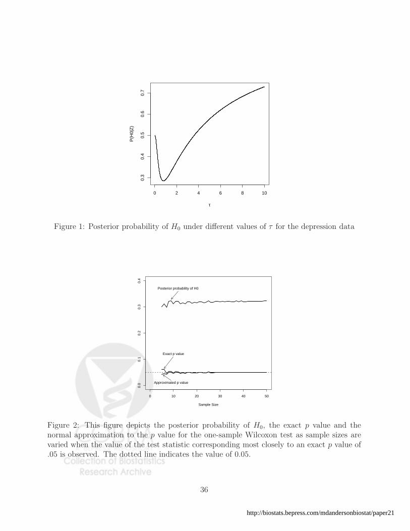
the null hypothesis obtained for different choices of τ are presented in Figure 1.

2.2 Bayes factors for nonparametric test statistics having limiting

χ2 distributions

When testing for differences between the distribution of values obtained from three or more

populations, most nonparametric test statistics do not have a limiting normal distribution.

Instead, their limiting distribution is often χ2. Such is the case for the Kruskal-Wallis test in

19


one-way ANOVA problems and Friedman’s test in two-way ANOVA settings. We illustrate

the extension of our methodology to such settings in the context of the Kruskal-Wallis test

(Kruskal and Wallis, 1952).

The Kruskal-Wallis test is a direct generalization of the two-sided Wilcoxon two-sample

test to the k ≥ 3 sample location problem. Let X11, . . . , X1n1, . . . , Xk1, . . . , Xknk

denote k

independent samples from continuous distributions F (x − θ1), . . . , F (x − θk), respectively,

where θ1, . . . , θk denote medians of the k populations. Let the total sample size be n =

∑ki=1 ni. We wish to test

H0 : θ1 = · · · = θk

versus

H1 : θi 6= θj for some 1 ≤ i, j ≤ k.

If Rij denotes the rank of Xij among X11, . . . , X1n1, . . . , Xk1, . . . , Xknk

, then the Kruskal-

Wallis statistic W is defined as

W =12

n(n + 1)

k∑

i=1

ni

(R̄i −

n + 1

2

)2

where R̄i is the average of the ranks associated with the ith sample, i.e.,

R̄i =1

ni

ni∑

j=1

Rij .

Under H0, W has an asymptotic χ2 distribution with k − 1 degrees of freedom as all

ni → ∞ simultaneously (Kruskal and Wallis, 1952). Because the statistic W test is consis-

tent against fixed alternatives, we again consider testing H0 against the sequence of local

alternatives

H1(n) : θi = θ0 + ∆i/√

n, i = 1, . . . , k (5)

20


where the {∆i} are not all equal. Assuming ni/n → ai > 0 where ai is a constant for

i = 1, . . . , k, Andrews (1954) showed that under H1(n) the limiting distribution of W is a

χ2k−1(ρ) distribution with non-centrality parameter

ρ = 12

{∫ ∞

−∞f 2(x) dx

}2 k∑

i=1

ai(∆i − ∆̄)2

and

∆̄ =k∑

i=1

ai∆i.

The non-centrality parameter ρ can be written as a quadratic form according to

ρ = 12

{∫ ∞

−∞f 2(x) dx

}2

∆′

P′

QP∆

where

∆ =

∆1

...

∆k

, P = I −

a1 · · · ak

......

a1 · · · ak

, Q =

a1 0 0

0. . . 0

0 0 ak

.

Because P′

QP is a non-negative definite matrix with rank k − 1, there exists a nonsingular

k × k matrix R such that

P′

QP = R′

Ik−1 0

0 0

R.

To obtain a Bayes factor based on W , it is necessary to assume a prior distribution

on ∆. A convenient prior for this purpose can be obtained by assuming that ∆ follows a

multivariate normal distribution of the form

∆ ∼ Nk(0, c(R′

R)−1) (6)

21


where c is a scaling constant.

Letting τ = 12c[∫ ∞

−∞ f 2(x) dx]2

, it follows that τ−1ρ follows a χ2 distribution with k− 1

degrees of freedom. The conditional distribution of W given ρ, say p(W |ρ), is thus a χ2k−1(ρ)

distribution, and the prior distribution on ρ, say π(ρ), is a scaled χ2 distribution τχ2k−1. It

follows that the marginal distribution of W under H1(n) can be expressed

m1(W ) =

∫ ∞

0

p(W |ρ)π(ρ) dρ

= Ga

[W |k − 1

2,

1

2(τ + 1)

]. (7)

Thus, the Bayes factor based on W is

BF01(W ) =Ga(W |k−1

2, 1

2)

Ga(W |k−12

, 12(τ+1)

)

= (τ + 1)k−1

2 exp

{− τW

2(τ + 1)

}. (8)

The value of τ that maximizes m1(W ) in (7) is

τ =W − (k − 1)

k − 1,

provided that W exceeds its expectation under H0. Setting τ at this value, we obtain the

upper bound of the Bayes factor against H0,

B̃F 01(W ) =

(W

k − 1

)k−1

2

exp

{−W − (k − 1)

2

}.

As before, this Bayes factor (8) is not consistent against local alternatives H1(n). How-

ever, the consistency of Bayes factor can be achieved if the values of two components of θ

are bounded away from each other under the alternative hypothesis. Such a constraint can

22


be imposed by replacing the prior distribution in (6) by an assumption that

∆ ∼ Nk(0, cn(R′

R)−1).

In this case, the Bayes factor is given by

BF01(W ) = (nτ + 1)k−1

2 exp

{− nτW

2(nτ + 1)

},

which is consistent as n → ∞.

Generalizations to other nonparametric test statistics that have limiting χ2 distributions

under the null hypothesis can be derived in a similar way. For example, Friedman’s test

statistic (Friedman, 1937) can be applied to randomized complete block designs when sub-

jects are divided into homogeneous blocks and it is of interest to compare subjects receiving

different treatments within blocks. Under the null hypothesis that all treatment effects are

equal, Friedman’s statistic has a limiting χ2 distribution. Under local alternatives similar to

(5) (where not all treatment effects are equal), Friedman’s statistic also follows a limiting

noncentral χ2 distribution (Elteren and Noether, 1959), and so the methods illustrated above

for the Kruskal-Wallis test can be applied. The resulting Bayes factor has a form similar to

(8).

3 Extensions to Meta-analyses

Our approach to Bayesian hypothesis testing provides an alternative to traditional meta-

analysis methods for combining evidence across studies. Our approach is especially useful

when study effect sizes are not reported but values of test statistics or p-values are, or when

study designs or treatment levels are so different that combining effect sizes is inappropriate.

23


A Bayesian meta-analysis using test statistics (or p-values) proceeds as follows. For

simplicity, we restrict attention here to the case in which all studies are based the same

test (e.g., the log-rank test) or in which the non-centrality parameters of all tests can be

transformed to a scale upon which they have a common interpretation. For concreteness,

we consider the case of test statistics that have asymptotic normal distributions; results

for test statistics having χ2 distributions follow along similar lines. Let T1, · · · , Ts denote

the values of the test statistic from s independent studies. It follows that the asymptotic

distribution of T = {T1, · · · , Ts} under H0, say m0(T ), is that of the product of s independent

standard normal random variables. Under H1, the marginal distribution of T , say m1(T ), is

obtained by averaging over the common prior distribution on the non-centrality parameter

∆. Following the reasoning of Section 2.1, we specify that the prior distribution for ∆ is

N(0, τ 2). Under the assumptions of Theorem 1, it follows that m1(T ) can be expressed

m1(T ) =

∫p(T1, · · · , Ts|∆)p(∆) d∆

=

∫p(T1|∆) · · ·p(Ts|∆)p(∆) d∆

= (1 + sC2τ 2)−1

2 (2π)−s2 exp

{−1

2

[∑Ti

2 − s2C2τ 2

1 + sC2τ 2(T̄ )2

]}

where T̄ =∑s

i=1 Ti/s.

The Bayes factor arising from the test statistics reported in the s studies is therefore

BF01(T ) =m0(T )

m1(T )

= (1 + sC2τ 2)1/2exp

[− s2C2τ 2(T̄ )

2

2(1 + sC2τ 2)

].

Minimizing this expression with respect to (a common) τ , we find that the upper bound of

24


the Bayes factor against the null hypothesis is

B̃F 01(T ) = s1

2 |T̄ | exp

[1 − s|T̄ |2

2

]. (9)

The next example provides an illustration of this methodology by combining evidence from

several studies in which log-rank tests were used to summarize evidence against the null

hypothesis.

Meta-analysis comparing two chemotherapies of ovarian cancer

The Ovarian Cancer Meta-analysis Project (1991) undertook a meta-analysis of ovarian

cancer treatments based on four published randomized clinical trials that compared two

regimens of chemotherapy for ovarian carcinoma: cyclophosphamide plus cisplatin (CP), and

cyclophosphamide, doxorubicin and cisplatin (CAP). Table 2 displays the logrank statistics

(O−E√V

) reported from the four studies. Each statistic was based on a comparison of survival

times in the treatment of ovarian carcinoma using CP or CAP. None show a significant

survival benefit between CP and CAP in 5% tests. To combine evidence from these four

trials, a meta-analysis project was conducted to retrospectively collect information from all

1194 individual patients in all four trials. Information from the four trials was pooled, and a

stratified log-rank test in which studies were treated as stratum was conducted. The results

from the meta-analysis are summarized in the last line of Table 2. The classical meta-analysis

suggested a significant survival benefit for CAP (p value =.02), concluding that CAP was

significantly better than CP. This approach, the so-called meta-analysis of individual patient

data (IPD), required the retrieval of individual patient records from trial investigators, and

was thus very time consuming and resource intensive. In more typical meta-analysis, only

25


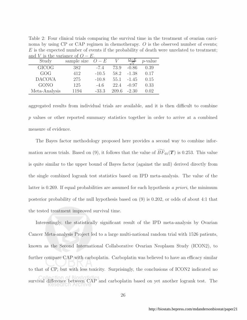
Table 2: Four clinical trials comparing the survival time in the treatment of ovarian carci-noma by using CP or CAP regimen in chemotherapy. O is the observed number of events;E is the expected number of events if the probability of death were unrelated to treatment;and V is the variance of O − E.

Study sample size O − E V O−E√V

p-value

GICOG 382 -7.4 73.9 -0.86 0.39GOG 412 -10.5 58.2 -1.38 0.17

DACOVA 275 -10.8 55.1 -1.45 0.15GONO 125 -4.6 22.4 -0.97 0.33

Meta-Analysis 1194 -33.3 209.6 -2.30 0.02

aggregated results from individual trials are available, and it is then difficult to combine

p values or other reported summary statistics together in order to arrive at a combined

measure of evidence.

The Bayes factor methodology proposed here provides a second way to combine infor-

mation across trials. Based on (9), it follows that the value of B̃F 01(T ) is 0.253. This value

is quite similar to the upper bound of Bayes factor (against the null) derived directly from

the single combined logrank test statistics based on IPD meta-analysis. The value of the

latter is 0.269. If equal probabilities are assumed for each hypothesis a priori, the minimum

posterior probability of the null hypothesis based on (9) is 0.202, or odds of about 4:1 that

the tested treatment improved survival time.

Interestingly, the statistically significant result of the IPD meta-analysis by Ovarian

Cancer Meta-analysis Project led to a large multi-national random trial with 1526 patients,

known as the Second International Collaborative Ovarian Neoplasm Study (ICON2), to

further compare CAP with carboplatin. Carboplatin was believed to have an efficacy similar

to that of CP, but with less toxicity. Surprisingly, the conclusions of ICON2 indicated no

survival difference between CAP and carboplatin based on yet another logrank test. The

26


p value for the second study was 0.98 (ICON collaborators, 1998). Possible explanations

for this apparent discrepancy between studies are discussed by Buyse et al. (2003). Our

interpretation is simpler: Evidence contained in the original studies for a treatment effect

was equivocal and was, unfortunately, overstated.

Actually, based on the reported logrank test statistics, the evidence contained in the

original four studies can be combined easily with ICON2 by our approach. In contrast,

IPD meta-analysis cannot be performed unless the individual patient information of ICON2

can be retrieved. Our method yields B̃F 01(T ) of 0.384, or odds of about 5:2 that CAP

improves survival time if equal probabilities are assumed for each hypothesis a priori. The

combination of studies still supports a treatment effect, although the magnitude of the effect

(based on MMLE of τ) is likely to be small.

4 Comparison of p values and Bayes factors

For one reason or another, Neyman-Pearson tests are typically conducted to bound Type

I error rates at 5%. In this section, we examine the values of Bayes factors obtained from

several nonparametric test statistics when those statistics fall on the boundary of their 5%

critical region. We also briefly examine the accuracy of the large sample approximation to

several nonparametric test statistics and the accuracy of this approximation on resultant

Bayes factors.

We first consider the one-sample Wilcoxon test, and assume that the null and alternative

hypotheses are assigned equal odds a priori. For this test statistic, Figure 2 displays (a)

the lower bound on the probability of the null hypothesis under the class of alternative

27


hypotheses specified in Section 2, (b) the exact p value, and (c) the p value based on the

large sample normal approximation. To the extent possible, the test statistic was chosen to

fall exactly on the boundary of the 5% critical region; if such a value could not be achieved,

we chose the value of the test statistic that resulted in the p value closest to 0.05. For sample

sizes larger than 15, Figure 2 shows that p values based on asymptotic approximations are

very close to their nominal values, and that the value of P̃ (H0|x) is quite stable.

Interestingly, the value of P̃ (H0|x) is approximately 0.3 for all sample sizes. Thus, a p

value of 0.05 corresponds to at least a 30% probability that the null hypothesis is true for

this class of alternative hypotheses when null and alternative hypotheses are assigned equal

weight a priori. To achieve “agreement” between the p value and the posterior probability

of the null model, i.e., to have P̃ (H0|x) = 0.05 when the p value is 0.05, the prior probability

assigned to the null hypothesis must be approximately 0.15. These results are comparable to

those reported by Beger and Delampady (1987) and Johnson (2005). The relation between p

values and Bayes factors based on the Wilcoxon one-sample test statistic is explored further

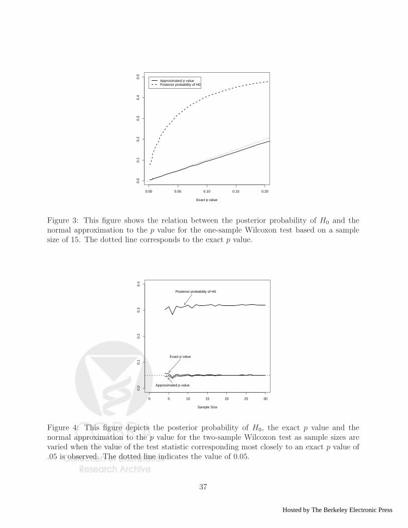
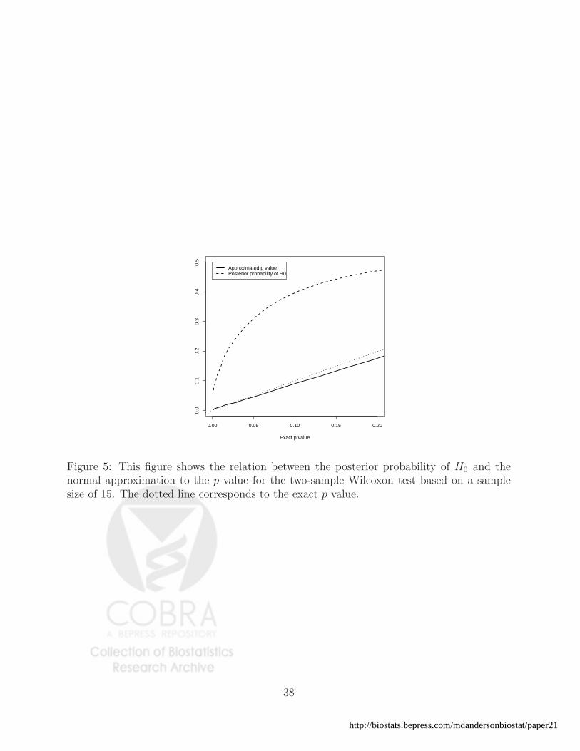
in Figure 3, where we plot P̃ (H0|x) versus different exact p values for a sample size of 15.

Exact p values were obtained from tables contained in Wilcoxon, Katti and Wilcox (1973).

Figures 4 and 5 show similar comparisons for the Mann-Whitney-Wilcoxon test.

5 Conclusion

Traditionally, the application of Bayesian testing procedures to classical nonparametric set-

tings has been restricted due to the absence of sampling densities for the data. In this article,

we have demonstrated how this difficulty can be circumvented by modeling the distribution

28


of test statistics directly. Use of this methodology allows scientists to summarize the results

of tests in terms of model probabilities and Bayes factors rather than p values, and thereby

represents an important advance in the field of nonparametric statistical hypothesis testing.

By reducing the subjectivity typically associated with the use of Bayes factors, it should

also alleviate objections from those who prefer more classical procedures. Finally, the use

of our methods has the potential for greatly simplifying the process of combining evidence

from independent studies in favor of various statistical hypotheses.

Methodology proposed in this article relies on asymptotic approximations to the distri-

bution of common nonparametric test statistics. However, numerical evidence presented in

Section 4 suggests that Bayes factors based on such approximations are not particularly

sensitive to the large sample approximations to the distributions of common test statistics.

For both one-sample and two-sample Wilcoxon tests, our method appears to give accurate

results for sample sizes larger than 15. This figure is consistent with recommendations for

the application of large sample approximations cited by Gibbons and Chakraborti (2003).

6 Appendix

6.1 Proof of Theorem 1

T ∗k =

Tk − µ(θ0)

σk(θ0)=

Tk − µ(θk) + µ(θk) − µ(θ0)

σk(θ0)

≃ Tk − µ(θk) + µ′

(θ0)(θk − θ0)

σk(θ0)

=Tk − µ(θk)

σk(θ0)+

µ′

(θ0)√nkσk(θ0)

∆

29


Now,

Tk − µ(θk)

σk(θ0)=

Tk − µ(θk)

σk(θk)

σk(θk)

σk(θ0)L−→ N(0, 1),

so application of Slutsky’s theorem gives the desired result.

6.2 Proof of Theorem 3

Taking the logarithm of (4) we obtain

log(BF01) =1

2log(1 + C2τ 2nk) −

C2nkτ2T ∗

k2

2(1 + C2nkτ 2).

If H0 is true, T ∗k

2 has an asymptotic χ2 distribution with 1 degree of freedom, so the second

term is bounded in probability. Since the first term is O(log(nk)), it follows that log(BF01) →

∞.

If H1 is true, log(BF01) can be rewritten as

log(BF01) =1

2log(1 + C2τ 2nk) −

1

2C2nkτ

2

(T ∗

k√1 + C2nkτ 2

)2

Because(

T ∗k√

1 + C2nkτ 2

)2

has an asymptotic χ2 distribution with 1 degree of freedom, it is bounded probability. The

second term is O(nk). Since the first term is O(log(nk)), it follows that log(BF01) → −∞.

30


References

[1] Andrews, F. C. (1954), Asymptotic behavior of some rank tests for analysis of variance.

Annals of Mathematical Statisitics, 25, 724-736

[2] Buyse, M., Burzykowski, T. and et al. (2003), Using the expected survival to explain

differences between the results of randomized trials: a case in advanced ovarian cancer.

Journal of Clinical Oncology, 21, 1682-1687

[3] Berger, J. O. (1985) Statistical Decision Theory and Bayesian Analysis, 2nd edn. New

York: Springer.

[4] Berger, J. O. and Delampady, M. (1987), Testing precise Hypotheses (with discussions).

Statistical Science, 2, 317-352

[5] Berger, J. O. and Sellke, T. (1987), Testing a point null hypothesis: the irreconcilability

of p value and evidence. Journal of American statistical Association, 82, 112-122

[6] Casella, G. and Berger, R. L. (1987), Reconciling bayesian and frequentist evidence in

the one-sided testing problem. Journal of American statistical Association, 82, 106-111

[7] Chernoff, H. and Savage, I. R. (1958), Asymptotic normality and efficiency of certain

nonparametric test statistics. Annals of Mathematical Statisitics, 29, 972-994.

[8] Dickey, J. M. (1977), Is the tail area useful as an approximate bayes factor? Journal of

American statistical Association, 72, 138-142

31


[9] Edwards, W., Lindman, H. and Savage, L. J. (1963) Bayesian statistical inference for

psychological research. Psychological Review, 70, 193242.

[10] Elteren, P. V. and Noether, G. E. (1959), The asymptotic efficiency of the χ2r-test for a

balanced incomplete block design. Biometrika, 46, 475-477

[11] Fisher, R.A. (1956). Statistical methods and scientific inference, Edinburgh: Oliver and

Boyd.

[12] Fleming, T. R. and Harrington, D. P. (1991), Counting process and survival analysis.

John Wiley & Sons.

[13] Friedman, M. (1937), The use of ranks to avoid the assumption of normality implicit in

the analysis of variance. Journal of American Statistical Association, 32, 675-699

[14] Gibbons, J. D. and Chakraborti, S. (2003), Nonparametric statistical inference. Marcel

Dekker, Inc.

[15] Gill, R. D. (1980), Censoring and stochastic integrals. Mathematical Centre Tracts 124,

Mathematisch Centrum, Amsterdam

[16] Good, I. J. (1950) Probability and the Weighting of Evidence. London: Griffin.

[17] Good, I. J. (1958) Significance tests in parallel and in series. Journal of American

Statistical Association, 53, 799813.

[18] Good, I. J. (1967) A Bayesian significance test for multinomial distributions (with dis-

cussion). Journal of the Royal Statistical Society: Series B, 29, 399431.

32


[19] Good, I. J. (1986) The maximum of a Bayes factor against ’independence’ in a contin-

gency table, and generalizations to higher dimensions. Journal of Statistical Computing

and Simulation, 26, 312316.

[20] Goodman, S. N. (1999a), Toward evidence-based medical statistics. 1: the p value

fallacy. Annals of Internal Medicine, 130, 995-1004

[21] Goodman, S. N. (1999b), Toward evidence-based medical statistics. 2: the bayes factor.

Annals of Internal Medicine, 130, 1005-1013

[22] Goodman, S. N. (2001), Of p-values and bayes: a modest proposal. Epidemiology, 12,

295-297

[23] Hajek, J. (1961), Some extensions of the Wald-Wolfowitz-Noether theorem. Annals of

Mathematical Statisitics, 32, 506-523

[24] Hoeffding, W. (1948), A Class of Statistics with Asymptotical Normal Distribution.

Annals of Mathematical Statisitics, 19, 293-325

[25] Hollander M. and Wolfe D. A. (1999), Nonparametrics statistical Methods New York:

John Wiley & Sons.

[26] Jeffreys, H. (1961), Theory of Probability, Oxford University Press: London.

[27] Johnson, E. V. (2005), Bayes factor based on test statistics. Journal of the Royal Sta-

tistical Society: Series B, 67, 689-701.

33


[28] Kass, R. E. and Raftery, A. E. (1995), Bayes factors. Journal of American statistical

Association, 90, 773-795

[29] Kruskal, W. H. and Wallis, W. A. (1952), Use of ranks in one-criterion variance analysis.

Journal of American statistical Association, 47, 583-621

[30] Lehmann E. L. (1975), Nonparametrics: Statistical Methods Based on Ranks. San

Francisco: Holden-Day

[31] Lindley, D.V. (1957), A Statistical Paradox. Biometrika, 44, 187-192.

[32] Noether, G. E. (1955), On a theorem of Pitman. Annals of Mathematical Statisitics,

26, 64-68

[33] Ovarian Cancer Meta-Analysis Project (1991), Cyclophosphamide plus cisplatin versus

cyclophosphamine, doxorubicin and cisplatin chemotherapy of ovarian carcinoma: A

meta-analysis. Journal of Clinical Oncology, 9, 1668-1674

[34] Randles, R. H. and Wolfe, D. A. (1979), Introduction to the theory of nonparametric

statistics. New York, John Wiley & Sons

[35] Rousseau, J. (2006), “Bayes Factors in Nonparametric Statistics,” to appear in Pro-

ceedings of the 8th Valencia Conference on Bayesian Statistics.

[36] The ICON Collaborators (1998), ICON-2: A randomised trial of single-agent carbo-

platin agaist the 3-drug combination of CAP (cyclophosphamide, doxorubicin and cis-

platin) in women with ovarian cancer. Lancet, 352, 1571-1576

34


[37] Wilcoxon, F., Katti, S. K. and Wilcox, R. A. (1973), Critical values and probability

levels for the Wilcoxon rank sum test and the Wilcoxon signed rank test, In Selected

tables in mathematical statistics, volume 1. Edited by H.L. Harter and D.B. Owen. Prov-

idence, R. I.: American Mathematical Society and Institute of Mathematical Statistics,

pp. 171-260.

35


0 2 4 6 8 10

0.3

0.4

0.5

0.6

0.7

τ

P(H

0|Z

)

Figure 1: Posterior probability of H0 under different values of τ for the depression data

0 10 20 30 40 50

0.0

0.1

0.2

0.3

0.4

Sample Size

Posterior probability of H0

Exact p value

Approximated p value

Figure 2: This figure depicts the posterior probability of H0, the exact p value and thenormal approximation to the p value for the one-sample Wilcoxon test as sample sizes arevaried when the value of the test statistic corresponding most closely to an exact p value of.05 is observed. The dotted line indicates the value of 0.05.

36


0.00 0.05 0.10 0.15 0.20

0.0

0.1

0.2

0.3

0.4

0.5

Exact p value

Approximated p valuePosterior probability of H0

Figure 3: This figure shows the relation between the posterior probability of H0 and thenormal approximation to the p value for the one-sample Wilcoxon test based on a samplesize of 15. The dotted line corresponds to the exact p value.

0 5 10 15 20 25 30

0.0

0.1

0.2

0.3

0.4

Sample Size

Posterior probability of H0

Exact p value

Approximated p value

Figure 4: This figure depicts the posterior probability of H0, the exact p value and thenormal approximation to the p value for the two-sample Wilcoxon test as sample sizes arevaried when the value of the test statistic corresponding most closely to an exact p value of.05 is observed. The dotted line indicates the value of 0.05.

37


0.00 0.05 0.10 0.15 0.20

0.0

0.1

0.2

0.3

0.4

0.5

Exact p value

Approximated p valuePosterior probability of H0

Figure 5: This figure shows the relation between the posterior probability of H0 and thenormal approximation to the p value for the two-sample Wilcoxon test based on a samplesize of 15. The dotted line corresponds to the exact p value.

38


Documents

University of Texas, MD Anderson Cancer Center