University of Warwick institutional repository: http://go.warwick.ac.uk/wrap

A Thesis Submitted for the Degree of PhD at the University of Warwick

http://go.warwick.ac.uk/wrap/66024

This thesis is made available online and is protected by original copyright.

Please scroll down to view the document itself.

Please refer to the repository record for this item for information to help you to cite it. Our policy information is available from the repository home page.

ALGORITHMS FOR BREAST CANCER GRADING IN

DIGITAL HISTOPATHOLOGY IMAGES

by

Adnan Mujahid Khan

Thesis

Submitted to the University of Warwick

for the degree of

Doctor of Philosophy

Department of Computer Science

August 2014

Contents

List of Tables iv

List of Figures vi

Acknowledgments x

Declarations xii

List of Publications xiii

Abstract xvi

Abbreviations xviii

Chapter 1 Introduction 1

1.1 Diagnosis of Breast Cancer . . . . . . . . . . . . . . . . . . . . . . . . . . 4

1.2 Slide preparation, staining and digitisation . . . . . . . . . . . . . . . . . . 6

1.3 Histological grading of breast tissues for disease identification . . . . . . . 12

1.4 Aims of the thesis . . . . . . . . . . . . . . . . . . . . . . . . . . . . . . . 15

1.5 Thesis organisation . . . . . . . . . . . . . . . . . . . . . . . . . . . . . . 18

1.6 Description of the datasets used in this thesis . . . . . . . . . . . . . . . . 19

1.7 Summary . . . . . . . . . . . . . . . . . . . . . . . . . . . . . . . . . . . 22

Chapter 2 Stain Normalisation 24

i

2.1 Introduction . . . . . . . . . . . . . . . . . . . . . . . . . . . . . . . . . . 24

2.2 The Colour Deconvolution Model . . . . . . . . . . . . . . . . . . . . . . 33

2.3 Stain Normalisation Algorithm . . . . . . . . . . . . . . . . . . . . . . . . 34

2.4 Experimental Results . . . . . . . . . . . . . . . . . . . . . . . . . . . . . 44

2.5 Discussion . . . . . . . . . . . . . . . . . . . . . . . . . . . . . . . . . . . 52

2.6 Summary . . . . . . . . . . . . . . . . . . . . . . . . . . . . . . . . . . . 55

Chapter 3 Tumour Segmentation 57

3.1 Related Work . . . . . . . . . . . . . . . . . . . . . . . . . . . . . . . . . 57

3.2 Texture Features for Tumour Segmentation . . . . . . . . . . . . . . . . . 62

3.3 RanPEC: A Framework for Dimensionality Reduction and Clustering . . . 68

3.4 Baseline Tumour Segmentation Framework . . . . . . . . . . . . . . . . . 71

3.5 HyMaP Tumour Segmentation Framework . . . . . . . . . . . . . . . . . 76

3.6 Summary . . . . . . . . . . . . . . . . . . . . . . . . . . . . . . . . . . . 86

Chapter 4 Mitotic Cell Detection 88

4.1 Related Work . . . . . . . . . . . . . . . . . . . . . . . . . . . . . . . . . 88

4.2 Our Approach . . . . . . . . . . . . . . . . . . . . . . . . . . . . . . . . . 94

4.3 Gamma-Gaussian Mixture Model for Candidate Detection . . . . . . . . . 95

4.4 Context Aware Postprocessing . . . . . . . . . . . . . . . . . . . . . . . . 101

4.5 Cell Words: Cell level Modelling of Mitotic Cells . . . . . . . . . . . . . . 102

4.6 Parameters, Experimental Setup & Evaluation . . . . . . . . . . . . . . . . 106

4.7 Results and Discussion . . . . . . . . . . . . . . . . . . . . . . . . . . . . 109

4.8 Summary . . . . . . . . . . . . . . . . . . . . . . . . . . . . . . . . . . . 115

Chapter 5 Nuclear Atypia Scoring 117

5.1 Baseline Framework for Nuclear Atypia Scoring . . . . . . . . . . . . . . . 120

5.2 The Proposed Framework . . . . . . . . . . . . . . . . . . . . . . . . . . . 127

5.3 Experimental Results and Discussion . . . . . . . . . . . . . . . . . . . . . 134

ii

5.4 Summary . . . . . . . . . . . . . . . . . . . . . . . . . . . . . . . . . . . 146

Chapter 6 Conclusions and Future Directions 148

6.1 Main Contributions . . . . . . . . . . . . . . . . . . . . . . . . . . . . . . 149

6.2 Future Directions . . . . . . . . . . . . . . . . . . . . . . . . . . . . . . . 152

Bibliography 156

iii

List of Tables

1.1 Various methods for collecting biopsy slides . . . . . . . . . . . . . . . . . 5

1.2 Specifications of commonly used bright-field microscopy digital whole-

slide scanners . . . . . . . . . . . . . . . . . . . . . . . . . . . . . . . . . 10

1.3 Nottingham criteria for breast cancer grading . . . . . . . . . . . . . . . . 13

1.4 Dataset used for evaluation of algorithms proposed in this research . . . . . 19

2.1 Rules for categorising an image into 3 classes: STAINED, OTHER, BACK-

GROUND . . . . . . . . . . . . . . . . . . . . . . . . . . . . . . . . . . . 43

2.2 5-Fold cross validation accuracy statistics for RVM classifier trained on a

single image and tested on 48 images from different tissue batches . . . . . 48

2.3 Run times for stain normalisation of images of various sizes . . . . . . . . 52

3.1 Quantitative evaluation of tumour segmentation on MITOS (Aperio) dataset 84

3.2 Quantitative evaluation of tumour segmentation on MITOS (Hamamatsu)

dataset . . . . . . . . . . . . . . . . . . . . . . . . . . . . . . . . . . . . . 84

3.3 Quantification of effect of stain normalisation on tumour segmentation ac-

curacy . . . . . . . . . . . . . . . . . . . . . . . . . . . . . . . . . . . . . 85

4.1 Results of MITOS contest for mitotic cell detection in BC histopathology

images . . . . . . . . . . . . . . . . . . . . . . . . . . . . . . . . . . . . . 111

4.2 Quantitative Comparison of CAPP and cell words algorithms on MITOS

dataset . . . . . . . . . . . . . . . . . . . . . . . . . . . . . . . . . . . . . 111

iv

4.3 Performance of the proposed algorithm on training/test splits of various

sizes on WarMiCe dataset . . . . . . . . . . . . . . . . . . . . . . . . . . . 112

4.4 Run times of the various components of the proposed mitotic cell detection

framework . . . . . . . . . . . . . . . . . . . . . . . . . . . . . . . . . . . 115

5.1 Texture Information measures on grey-level co-occurrence matrix . . . . . 123

5.2 Comparative %age classification accuracy results of nuclear atypia scoring

on baseline features using a range of classifiers . . . . . . . . . . . . . . . 137

5.3 Comparative %age classification accuracy results of RC and mSPD descrip-

tors using a range of classifiers on images from two different scanners . . . 137

5.4 Confusion matrices obtained when baseline Haralick descriptor was used

in conjunction with (a) DT, (b) RUSBoost, and (c) LDA classifiers . . . . . 138

5.5 Comparison of nuclear atypia scoring by the proposed system and three

pathologists . . . . . . . . . . . . . . . . . . . . . . . . . . . . . . . . . . 139

5.6 Comparison of computational efficiency of various descriptors and classi-

fiers used for nuclear atypia scoring . . . . . . . . . . . . . . . . . . . . . 140

5.7 Effect of preprocessing steps on the performance of the proposed nuclear

atypia scoring framework on Aperio Images . . . . . . . . . . . . . . . . . 145

5.8 Effect of preprocessing steps on the performance of the proposed nuclear

atypia scoring framework on Hamamatsu Images . . . . . . . . . . . . . . 146

v

List of Figures

1.1 Anatomy of Breast . . . . . . . . . . . . . . . . . . . . . . . . . . . . . . 2

1.2 Methods for diagnosing BC using mammography, breast ultrasound, and

X-ray guided needle biopsy . . . . . . . . . . . . . . . . . . . . . . . . . . 3

1.3 Example of a BC histopathology image obtained by digitising a glass slide

using a whole-slide scanner . . . . . . . . . . . . . . . . . . . . . . . . . . 8

1.4 Example IHC stained histopathology image of breast tissue captured using

Canon R© EOS D1100 mounted on a standard microscopes . . . . . . . . . . 9

1.5 Image acquisition platforms for bright-field microscopy . . . . . . . . . . . 11

1.6 Examples showing various kinds of artefacts in histological images pro-

duced by the whole-slide imaging devices . . . . . . . . . . . . . . . . . . 12

1.7 Snapshots showing different appearances of pleomorphic cells marked in

green colour . . . . . . . . . . . . . . . . . . . . . . . . . . . . . . . . . . 13

1.8 Snapshot showing tubular structures in a histological image . . . . . . . . . 14

1.9 Snapshots showing different appearances of mitotic cells encircled in green

colour . . . . . . . . . . . . . . . . . . . . . . . . . . . . . . . . . . . . . 15

2.1 Some histological images, chosen from our datasets, demonstrating varia-

tion in staining . . . . . . . . . . . . . . . . . . . . . . . . . . . . . . . . 25

2.2 Results of stain normalisation on histological images, presented in Figure

2.1 using the stain normalisation framework presented in this chapter . . . . 26

2.3 Evaluation of existing colour normalisation algorithms . . . . . . . . . . . 31

vi

2.4 Overview of the proposed stain normalisation algorithm . . . . . . . . . . . 35

2.5 Stain Matrix Estimation using colour classification . . . . . . . . . . . . . 37

2.6 Stability of SCDs before and after stain normalisation . . . . . . . . . . . . 39

2.7 Probability maps P(sn) for H&E and H&DAB stained images using classi-

fiers with no SCD and 1D SCD, respectively . . . . . . . . . . . . . . . . . 41

2.8 Marginal distributions of pixels belonging to STAINED, OTHER, BACK-

GROUND classes from a single channel . . . . . . . . . . . . . . . . . . . 42

2.9 B-Spline mapping function from reference image statistics to source image

statistics . . . . . . . . . . . . . . . . . . . . . . . . . . . . . . . . . . . . 44

2.10 Performance of Random Forest and RVM classifiers on pixel classification

in RGB and Lab colour spaces . . . . . . . . . . . . . . . . . . . . . . . . 45

2.11 Effect of Tp on stain vector estimation . . . . . . . . . . . . . . . . . . . . 47

2.12 Comparative results of proposed stain normalisation method with existing

methods . . . . . . . . . . . . . . . . . . . . . . . . . . . . . . . . . . . . 50

2.13 DICE Coefficient representing the agreement between algorithm’s output

and pathologist’s markings of Aperio and Hamamatsu HPF images . . . . 51

2.14 Demonstration of the need for image-specific stain matrix . . . . . . . . . . 54

3.1 Annotation of tumour and non-tumour regions in a BC histopathology image 61

3.2 Visual demonstration of tumour segmentation on a sample image using 3

different randomly generated projection matrices . . . . . . . . . . . . . . 70

3.3 Overview of the Baseline tumour segmentation framework . . . . . . . . . 72

3.4 Comparative results of pixel level classification accuracy (%) versus dimen-

sionality of the feature space for mRMR and RanPEC . . . . . . . . . . . . 75

3.5 A sample H&E stained BC histopathology image . . . . . . . . . . . . . . 77

3.6 Overview of the proposed HyMaP tumour segmentation algorithm . . . . . 78

3.7 Illustration of complimentary segmentations obtained by HypoCS and Hy-

perCS segmentation . . . . . . . . . . . . . . . . . . . . . . . . . . . . . . 81

vii

3.8 Visual results of tumour segmentation on two sample images . . . . . . . . 82

4.1 Visual appearance of different cells in breast histopathological images . . . 92

4.2 The proposed mitotic cells detection framework . . . . . . . . . . . . . . . 96

4.3 Marginal distributions and fitted models on MITOS (Aperio) dataset by the

two-component Gamma-Gaussian Mixture Model . . . . . . . . . . . . . . 98

4.4 Marginal distributions and fitted models on MITOS (Hamamatsu) dataset

by the two-component Gamma-Gaussian Mixture Model . . . . . . . . . . 98

4.5 Selecting appropriate threshold for binarisation of probability map obtained

from GGMM . . . . . . . . . . . . . . . . . . . . . . . . . . . . . . . . . 101

4.6 Four examples of 50 × 50 context patches, cropped around the bounding

box of candidate mitotic cells . . . . . . . . . . . . . . . . . . . . . . . . 102

4.7 Demonstration of candidate patch alignment on WarMiCe dataset . . . . . 107

4.8 Relative performance of GGMM model on the MITOS (Aperio) dataset

compared to manual and Otsu thresholding . . . . . . . . . . . . . . . . . 110

4.9 Snapshot of the false positive and false negative mitotic cells . . . . . . . . 112

4.10 Visual results of mitotic cells detection in a sample image taken from MI-

TOS (Aperio) dataset . . . . . . . . . . . . . . . . . . . . . . . . . . . . . 113

5.1 Visual appearance of different nuclei in breast histological images. Score-1

(top row), 2 (middle row), and 3 (bottom row) nuclear atypia . . . . . . . . 118

5.2 Baseline algorithm for nuclear atypia scoring . . . . . . . . . . . . . . . . 121

5.3 An example of computing LBP in a 3× 3 neighbourhood . . . . . . . . . . 124

5.4 An illustration of the overall classification framework using (top) the region

covariance and (bottom) generalised geometric mean of region covariance

descriptors . . . . . . . . . . . . . . . . . . . . . . . . . . . . . . . . . . . 128

5.5 Response of MR8 filter bank on a sample image from MITOS-Atypia dataset136

5.6 Demonstration of nuclear atypia scoring difficulty . . . . . . . . . . . . . . 141

5.7 Demonstration results of tumour segmentation on two MITOS-Atypia images144

viii

Dedicated to my parents Zaman and Naseem,

my wife Zainab and my son Ahmed.

ix

Acknowledgments

To Dr. Nasir Rajpoot for being, not only a great advisor, but also a great friend who gave

me confidence in myself and my work throughout these years. I feel that I have learned

a lot from him, and this is not limited to academic matters; To my external and internal

examiners, Prof. Stephen Mckennaa and Dr. Victor Sanchez, for thoroughly reviewing my

research work and providing extremely useful feedback.

To the University of Warwick for Warwick Postgraduate Research Scholarship and

Department of Computer Science for partially funding my PhD; to my academic advisors,

Dr. Sara Kalvala, Prof. Chang-Tsun Li, for their inputs, valuable discussions and accessi-

bility; to the administrative staff members at the Department of Computer Science for their

support throughout these years; to Prof. Anwar Majeed Mirza, Dr. Hassan Amin and Dr.

Asifullah Khan, my former research and academic advisors at Ghulam Ishaq Khan Institute

and National University of Computers and Emerging Sciences (FAST-NUCES) in Pakistan

for providing invaluable guidance on my first research project.

To Prof David Epstein for continuously providing me invaluable guidance and sup-

port during my doctorate research; to Dr. Derek Magee, Dr. Darren Treanor, Dr. Michael

Khan, Dr. Hesham El-Daly, Dr. Emma Simmons, Dr. Asha Rupani, Dr. David Snead and

Dr. Naresh Chachlani for being very supportive collaborators; to Dr. Metin Gurcan and Dr.

Khalid Niazi for all their support during my stay at Ohio in 2012.

To my friend and colleague Korsuk Sirinukunwattana for all the enlightening dis-

cussions especially during the last year of my PhD; to the colleagues and friends with whom

I have shared good moments during these years: Shan-e-Ahmed Raza, Ahmad Humayun,

Nadeem Choudhary, Violeta Kovacheva, Samuel Jefferyes, Guannan Li, Nicholas Trahearn

x

and Mike T. Song. Special acknowledgements to Anti’s Halal food for tirelessly serving us

with delicious food throughout these years.

To my old friends Abdul Waheed Malik, Saad Hussain, Hassan Sajjad, Adeel Choud-

hary and Usman Adeel, who supported me throughout this time by sharing unforgettable

moments.

To my parents, for their unconditional love, support and care over the span of my

entire life; to my mother-in-law, who gave me and my wife enormous support by tirelessly

babysitting our son throughout this time; to my brother Sher Afzal for holding my hand

in the most difficult times; to my sister Attia and her husband Rizwan, for taking care of

me throughout my stay in Qatar; to the rest of my family especially my sisters, who were

always there for me despite my total negligence.

To my beloved wife Zainab for patience, support, encouragement and unwavering

loyalty over the past four years, even in the face of extremely difficult times and to my little

kid Ahmed, who is my ultimate driving force.

To all of you, thank you very much!

xi

Declarations

This thesis is submitted to the University of Warwick in support of my application for the

degree of Doctor of Philosophy. I declare that, except where acknowledged, the material

contained in the thesis is my own work, and has not been previously published for obtaining

an academic degree.

Adnan Mujahid Khan

August 13, 2014

xii

List of Publications

Journal Publications

1. Adnan M. Khan, Nasir Rajpoot, Darren Treanor, and Derek Magee. A non-linear

mapping approach to stain normalisation in digital histopathology images using image-

specific colour deconvolution. IEEE Transactions on Biomedical Engineering (TBME),

61(6):17291738, 2014.

2. Korsuk Sirinukunwattana, Adnan M. Khan, and Nasir Rajpoot. Cell Words: Mod-

elling the visual appearance of cells in histopathology images. Computerized Medi-

cal Imaging and Graphics, 2014.

3. Mitko Veta, Paul J. van Diest, Stefan M. Willems, Haibo Wang, Anant Madabhushi,

Angel Cruz-Roa, Fabio Gonzalez, Anders B. L. Larsen, Jacob S. Vestergaard, An-

ders B. Dahl, Dan C. Cirean, Jrgen Schmidhuber, Alessandro Giusti, Luca M. Gam-

bardella, F. Boray Tek, Thomas Walter, Ching-Wei Wang, Satoshi Kondo, Bogdan

J. Matuszewski, Frederic Precioso, Violet Snell, Josef Kittler, Teofilo E. de Campos,

Adnan M. Khan, Nasir M. Rajpoot, Evdokia Arkoumani, Miangela M. Lacle, Max

A. Viergever, and Josien P.W. Pluim. Assessment of algorithms for mitosis detection

in breast cancer histopathology images. Submitted to Medical Image Analysis, 2014.

4. Adnan M. Khan, Hesham ElDaly, and Rajpoot Nasir M. A Gamma-Gaussian mix-

ture model for detection of mitotic cells in breast cancer histopathology images. Jour-

nal of Pathology Informatics (JPI), 4(11), 2013.

5. Adnan M. Khan, Hesham El-Daly, Emma Simmons, and Nasir M Rajpoot. HyMaP:

xiii

A hybrid magnitude-phase approach to unsupervised segmentation of tumor areas in

breast cancer histology images. Journal of Pathology Informatics (JPI), 4(2), 2013.

6. Adnan M. Khan, Shan-e-Ahmad Raza, Mike Khan, Nasir Rajpoot. Cell phenotyp-

ing in multi-tag fluorescent bioimages. Neurocomputing, 134:254-261, 2014.

7. Violet N. Kovacheva, Adnan M. Khan, Mike Khan, David B.A. Epstein, Nasir Ra-

jpoot. DiSWOP: A novel measure for cell-level protein network analysis in localised

proteomics image data. Bioinformatics, 1-8, 2013. []

Conference Publications

1. Adnan M. Khan, Korsuk Sirinukunwattana, Nasir Rajpoot. Geodesic Geometric

Mean of Regional Covariance Descriptors as an Image-Level Descriptor for Nuclear

Atypia Grading in Breast Histology Images. In 5th International Workshop in Ma-

chine Learning and Medical Imaging (MLMI), 2014.

2. Nada Aloraidi, Korsuk Sirinukunwattana, Adnan M. Khan, Nasir Rajpoot. On Gen-

erating Cell Exemplars for Detection of Mitotic Cells in Breast Cancer Histopathol-

ogy Images. In 36th Annual International Conference of the IEEE Engineering in

Medicine and Biology Society (EMBS), 2014.

3. Adnan M. Khan, Aisha F Mohammed, Shama A Al-Hajri, HajerMAl Shamari,

Uvais Qidwai, Imaad Mujeeb, and Nasir Rajpoot. A novel system for scoring of

hormone receptors in breast cancer histopathology slides. In 2nd Middle East Con-

ference on Biomedical Engineering (MECBME), pages 155158. IEEE, 2014.

4. Adnan M. Khan, Hesham El-Daly, and Nasir Rajpoot. RanPEC: Random Projec-

tions with Ensemble Clustering for Segmentation of Tumor Areas in Breast Histol-

ogy Images. In Medical Image Understanding and Analysis (MIUA), pages 1723.

BMVA, 2012.

5. Adnan M. Khan, Ahmad Humayun, Shan-e-Ahmad Raza, Mike Khan and Nasir

Rajpoot. A Novel Paradigm for Mining Cell Phenotypes in Multi-Tag Bioimages

xiv

using a Locality Preserving Nonlinear Embedding. In 19th International Conference

on Neural Information Processing (ICONIP), pages 575-583. IEEE, 2012.

6. Adnan M. Khan, Mike Khan and Nasir Rajpoot. Towards Cell Level Protein In-

teraction in Multivariate Bioimages. In proceedings of the Qatar Foundation Annual

Research Conference (QARC), 2013.

7. Mehjabin Sultana Monjur, Shih Tseng, Adnan M. Khan, Nasir Rajpoot, and Selim

M Shahriar. Application of hybrid optoelectronic correlator to Gabor jet images for

rapid object recognition & segmentation. In CLEO: Science and Innovations. Optical

Society of America, 2013.

xv

Abstract

Histological analysis of tissue biopsies by an expert pathologist is considered gold standard

for diagnosing many cancers, including breast cancer. Nottingham grading system, which

is the most widely used criteria for histological grading of breast tissues, consists of three

components: mitotic count, nuclear atypia and tubular formation. In routine histological

analysis, pathologists perform grading of breast cancer tissues by manually examining each

tissue specimen against the three components, which is a laborious and subjective process

and thus can suffer from low inter-observer agreement. With the advent of digital whole-

slide scanning platforms, automatic image analysis algorithms can be used as a partial so-

lution for these issues. The main goal of this dissertation is to develop frameworks that can

aid towards building an automated or semi-automated breast cancer grading system. We

present novel frameworks for detection of mitotic cells and nuclear atypia scoring in breast

cancer histopathology images. Both of these frameworks can play a fundamental role in

developing a computer-assisted breast cancer grading system. Moreover, the proposed im-

age analysis frameworks can be adapted to grading and analysis of cancers of several other

tissues such as lung and ovarian cancers.

In order to deal with one of the fundamental problems in histological image analy-

sis applications, we first present a stain normalisation algorithm that minimises the staining

inconsistency in histological images. The algorithm utilises a novel image-specific colour

descriptor which summarises the colour contents of a histological image. Stain normalisa-

tion algorithm is used in the remainder of the thesis as a preprocessing step.

We present a mitotic cell detection framework mimicking a pathologist’s approach,

whereby we first perform tumour segmentation to restrict our search for mitotic cells to

xvi

tumour regions only, followed by candidate detection and evaluation in a statistical machine

learning framework. We also employ a discriminative dictionary learning paradigm to learn

the visual appearance of mitotic cells, that models colour, texture, and shape in a composite

manner.

Finally, we present a nuclear atypia scoring framework based on a novel image de-

scriptor which summarises the texture heterogeneity, inherent in histological images in a

compact manner. Classification is performed using a geodesic k-nearest neighbour clas-

sifier which explicitly exploits the structure of Riemannian manifold of the descriptor and

achieves significant performance boost as compared to Euclidean counterpart.

xvii

Abbreviations

1D 1-dimensional

2D 2-dimensional

3D 3-dimensional

BC Breast cancer

BR Blue ratio

CAPP Context-aware postprocessing

CD Colour deconvolution

DDL Discriminative dictionary learning

DR Dimensionality reduction

EM Expectation maximisation

ER Estrogen receptor

FN False negative

FP False positive

GMM Gaussian mixture model

GGMM Gamma-Gaussian mixture model

GkNN Geodesic k-nearest neighbour

GT Ground truth

H&E Hematoxylin & Eosin

H&DAB Hematoxylin & diaminobenzidine

HER2 Human epidermal growth factor 2

HPF High power field

HyperCS Hyper-cellular stroma

xviii

HypoCS Hypo-cellular stroma

IHC Immunohistochemical

kNN k-nearest neighbour

Lab CIE’s lab colour space

LBP Local binary patterns

LDA Linear discriminant analysis

mRMR Minimum redundancy maximum relevance

mSPD Generalised geometric mean of symmetric positive definite matrices

MI Mutual information

MLE Maximum likelihood estimate

OD Optical density

PCA Principal component analysis

PCH Principal colour histogram

PR Progestrone receptor

QDA Quadratic discriminant analysis

RanPEC Random projections with ensemble clustering

RC Region covariance

RF Random forest

RGB Red green blue

RPs Random projections

RVM Relevance vector machines

SCD Stain colour descriptor

SPD Symmetric positive definite

SVD Singular value decomposition

SVM Support vector machines

TMA Tissue microarray

TP True positive

TN True negative

UHCW University hospital Coventry and Warwickshire

WSI Whole-slide image

xix

Chapter 1

Introduction

Cancer refers to a group of diseases that occur as a result of abnormal changes in genes1

responsible for cell growth [1]. Under normal conditions, cells replace themselves through

a normal process of cell growth: new cells replace the dying cells. However, over the period

of time, these abnormal changes may regulate or deregulate certain genes, which may result

in cells dividing without control, producing more cell replicates and forming a tumour.

A tumour can be benign or malignant. Benign tumours are not considered cancer-

ous because the appearance of benign tumour cells is close to the appearance of normal

cells. Moreover, they grow slowly and they do not spread to other parts of the body. Malig-

nant tumours, on the other hand, are cancerous and have the potential to eventually spread

beyond the primary tumour to other2 parts of the body. If the malignant tumour is developed

from the cells in breast, it is called breast cancer (BC). BC can begin in three locations: (1)

Lobules, which are the milk producing glands; (2) Ducts, which are the passages that drain

milk from the lobules to the nipples; or (3) Stromal tissues, which include the fatty and

fibrous connective tissues of the breast (see Figure 1.1). Among the three locations, the first

two form the most prevalent class of BC. Following are some of the most common types of

BC [2, 3].1Genes are located in the DNA which is found in nucleus of cell. Genes are responsible for regulating

various activities of cell like cell growth and programmed cell death.2This phenomenon is often referred to as metastasis.

1

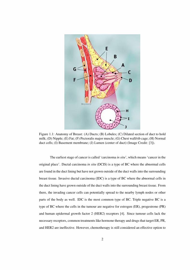
Figure 1.1: Anatomy of Breast: (A) Ducts; (B) Lobules; (C) Dilated section of duct to holdmilk; (D) Nipple; (E) Fat; (F) Pectoralis major muscle; (G) Chest wall/rib cage; (H) Normalduct cells; (I) Basement membrane; (J) Lumen (center of duct) (Image Credit: [3]).

The earliest stage of cancer is called ‘carcinoma in situ’, which means ‘cancer in the

original place’. Ductal carcinoma in situ (DCIS) is a type of BC where the abnormal cells

are found in the duct lining but have not grown outside of the duct walls into the surrounding

breast tissue. Invasive ductal carcinoma (IDC) is a type of BC where the abnormal cells in

the duct lining have grown outside of the duct walls into the surrounding breast tissue. From

there, the invading cancer cells can potentially spread to the nearby lymph nodes or other

parts of the body as well. IDC is the most common type of BC. Triple negative BC is a

type of BC where the cells in the tumour are negative for estrogen (ER), progestrone (PR)

and human epidermal growth factor 2 (HER2) receptors [4]. Since tumour cells lack the

necessary receptors, common treatments like hormone therapy and drugs that target ER, PR,

and HER2 are ineffective. However, chemotherapy is still considered an effective option to

2

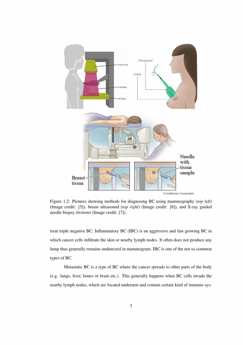
Figure 1.2: Pictures showing methods for diagnosing BC using mammography (top left)(Image credit: [5]), breast ultrasound (top right) (Image credit: [6]), and X-ray guidedneedle biopsy (bottom) (Image credit: [7]).

treat triple negative BC. Inflammatory BC (IBC) is an aggressive and fast growing BC in

which cancer cells infiltrate the skin or nearby lymph nodes. It often does not produce any

lump thus generally remains undetected in mammogram. IBC is one of the not so common

types of BC.

Metastatic BC is a type of BC where the cancer spreads to other parts of the body

(e.g. lungs, liver, bones or brain etc.). This generally happens when BC cells invade the

nearby lymph nodes, which are located underarm and contain certain kind of immune sys-

3

tem cells. Once malignant cells infiltrate the lymph nodes, there is a high likelihood that

they will infiltrate other parts of the body and subsequently grow tumour on other secondary

locations as well. The process which determines how far the cancer cells have spread be-

yond the primary location is called ‘cancer staging’3. For details regarding staging, inter-

ested reader is referred to the online article [8].

1.1 Diagnosis of Breast Cancer

In order to diagnose BC, three types of tests are generally performed at hospitals: (1) Mam-

mogram; (2) Breast ultrasound scans; or (3) Biopsy, as shown in Figure 1.2. A mammogram

is an X-ray of the breast and is routinely used as a basic tool for finding early changes in

the breast when it may be difficult to feel a lump. Although very effective in diagnosing BC

in older women, mammograms are not effective on younger women (under 35 years). This

is because the breasts of younger women are too dense to give a clear picture with mam-

mograms. Therefore, younger women are generally suggested to have a breast ultrasound,

where sound waves are used to get a picture of the inside of the breast [9].

A biopsy is done when imaging tests (mammograms/ultrasounds) and/or the physi-

cal examination find or suspect a breast abnormality. A biopsy is currently the only way to

confirm the presence of cancer. A breast biopsy is a procedure through which a small spec-

imen of tissue is extracted for microscopic analysis. The specimen is sent to a laboratory

where a pathologist examines it under the microscope and decides if the sample is cancer-

ous. Table 1.1 lists some of the most commonly used methods for collecting the biopsy

samples.

Histopathology is the microscopic examination of tissue for disease diagnosis. Specif-

ically, in clinical medicine, histopathology refers to the examination of a biopsy specimen

by a pathologist, after the specimen has been processed and histological sections have been3Note that staging is different from grading as grading determines how abnormal cancer cells appear, as

compared to normal cells, in a microscopic examination. There are five stages and three grades of BC. Wediscuss the process of BC grading in detail in Section 1.3.

4

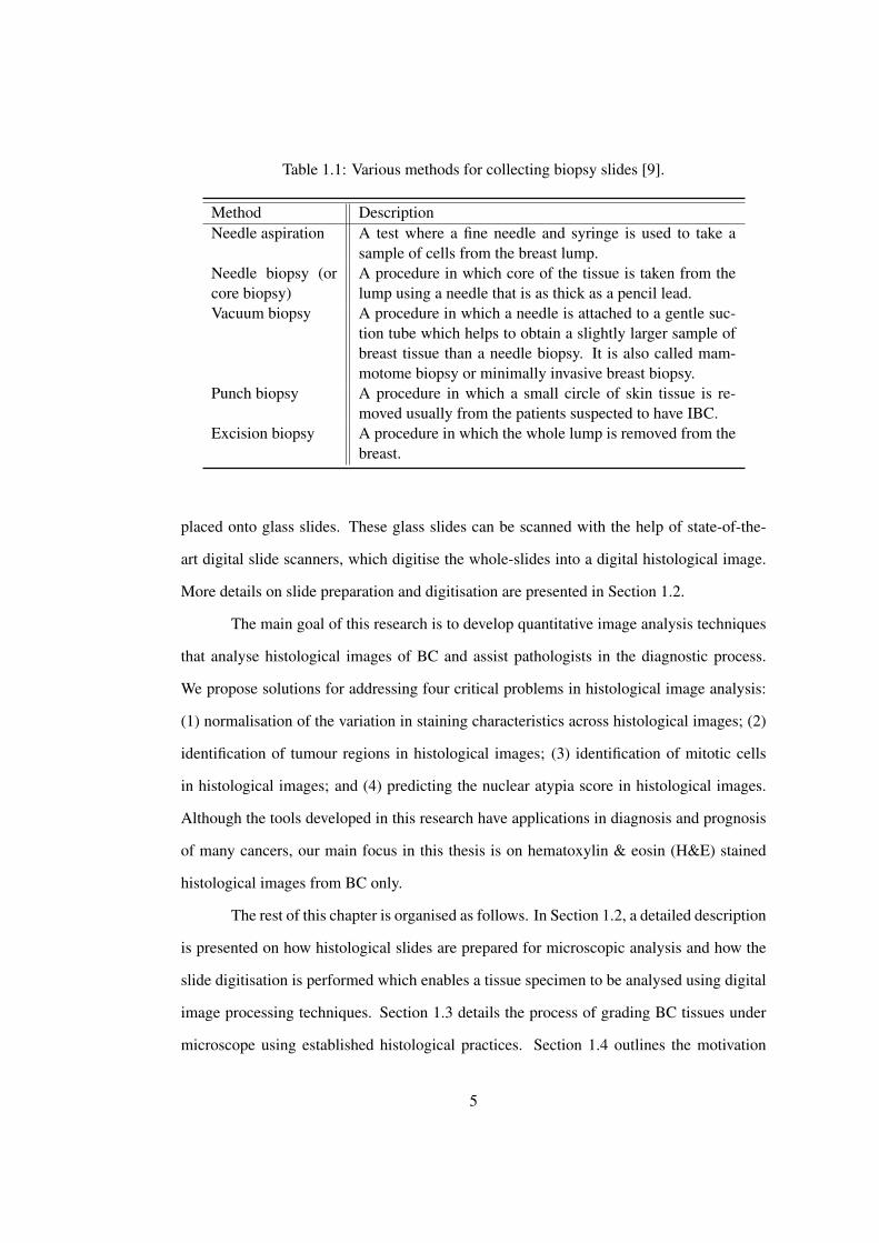
Table 1.1: Various methods for collecting biopsy slides [9].

Method DescriptionNeedle aspiration A test where a fine needle and syringe is used to take a

sample of cells from the breast lump.Needle biopsy (orcore biopsy)

A procedure in which core of the tissue is taken from thelump using a needle that is as thick as a pencil lead.

Vacuum biopsy A procedure in which a needle is attached to a gentle suc-tion tube which helps to obtain a slightly larger sample ofbreast tissue than a needle biopsy. It is also called mam-motome biopsy or minimally invasive breast biopsy.

Punch biopsy A procedure in which a small circle of skin tissue is re-moved usually from the patients suspected to have IBC.

Excision biopsy A procedure in which the whole lump is removed from thebreast.

placed onto glass slides. These glass slides can be scanned with the help of state-of-the-

art digital slide scanners, which digitise the whole-slides into a digital histological image.

More details on slide preparation and digitisation are presented in Section 1.2.

The main goal of this research is to develop quantitative image analysis techniques

that analyse histological images of BC and assist pathologists in the diagnostic process.

We propose solutions for addressing four critical problems in histological image analysis:

(1) normalisation of the variation in staining characteristics across histological images; (2)

identification of tumour regions in histological images; (3) identification of mitotic cells

in histological images; and (4) predicting the nuclear atypia score in histological images.

Although the tools developed in this research have applications in diagnosis and prognosis

of many cancers, our main focus in this thesis is on hematoxylin & eosin (H&E) stained

histological images from BC only.

The rest of this chapter is organised as follows. In Section 1.2, a detailed description

is presented on how histological slides are prepared for microscopic analysis and how the

slide digitisation is performed which enables a tissue specimen to be analysed using digital

image processing techniques. Section 1.3 details the process of grading BC tissues under

microscope using established histological practices. Section 1.4 outlines the motivation

5

behind the development of computer-aided diagnostic systems in histopathology, in general,

and the tools that we propose in this thesis, in particular. Section 1.5 briefly presents the

thesis organisation. Section 1.6 briefly describes the datasets used in this research followed

by a summary of the chapter in Section 1.7.

1.2 Slide preparation, staining and digitisation

Among different forms of microscopy, the one most commonly employed for histopathol-

ogy analysis is bright-field microscopy where the specimen is illuminated with a beam of

light that passes through it. In general, a specimen must adhere to the following conditions

for successful bright-field microscopic examination [10]: (1) various structures (e.g. cells

and extracellular components) present in the specimen are preserved; (2) the specimen is

transparent so that light (from bright-field microscope) can pass through it; (3) the speci-

men is thin enough to have only a single layer of cells; and (4) different components of the

specimen are counter-stained so that they can be distinguished easily.

There are four options for preparing a specimen for histological analysis: (1) squash

preparations; (2) smears; (3) whole-mounts; and (4) sections. In squash preparations, cells

are intentionally crushed to reveal cellular contents (e.g. chromosomes). A smear specimen

consists of cells suspended in a fluid (e.g. blood, semen) or individual cells that are aspirated

from a surface (e.g. cervix). In whole-mounts, an entire specimen is placed directly on

a microscopic slide as the specimen is sufficiently thin and small. In sections, however,

the specimen cannot be placed directly on a slide as it is not thin enough; therefore, it

is externally supported so as to cut thin slices from it (usually 3–5µm thick). Of these

options, only the whole-mounts and the sections satisfy all four requirements of successful

bright-field microscopic examination [10].

Whereas the whole-mounts can be directly used for microscopic analysis, sections

cannot. This is because it is extremely difficult to prepare thin slices (sections) from a

fresh tissue as it is very delicate and can be easily damaged. Two strategies are gener-

6

ally employed to support the process of cutting thin slices from the specimen: (1) After

being removed from the patient’s breast, the tissue is immediately frozen and kept frozen

while sections are cut using a microtome in a freezing chamber. Sections obtained using

this strategy are called the frozen sections; (2) Alternatively, specimens are embedded in a

chemical agent that converts the tissue into a solid material and facilitates the process of

cutting thin sections from it. Various agents can be used for this purpose, though paraffin

is the most popular embedding agent. Sections obtained using this strategy are called the

paraffin sections.

After the specimen is removed from the patient’s breast and before the sections are

prepared, the specimen needs to be preserved from the enzyme activity that may be occur-

ring in the tissue specimen. This is achieved by the process of fixation, which essentially

stops enzyme activity and hardens the tissue specimen. Therefore, it is recommended that

the process of fixation should be initiated immediately after the separation of the specimen

from its blood supply. Formaldehyde is the most widely used fixing agent, usually referred

to as formalin [10].

The cells and other extracellular structures making up most tissue specimen are

colourless. In order to reveal the structural details of the tissue specimen, some form of

staining is required. H&E are the universally used stains that serve as a starting point in

providing essential structural information. H&E staining colours chromatin rich nuclei as

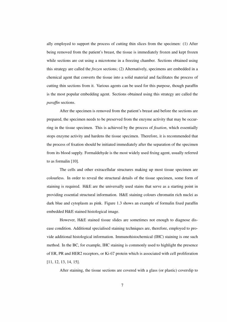
dark blue and cytoplasm as pink. Figure 1.3 shows an example of formalin fixed paraffin

embedded H&E stained histological image.

However, H&E stained tissue slides are sometimes not enough to diagnose dis-

ease condition. Additional specialised staining techniques are, therefore, employed to pro-

vide additional histological information. Immunohistochemical (IHC) staining is one such

method. In the BC, for example, IHC staining is commonly used to highlight the presence

of ER, PR and HER2 receptors, or Ki-67 protein which is associated with cell proliferation

[11, 12, 13, 14, 15].

After staining, the tissue sections are covered with a glass (or plastic) coverslip to

7

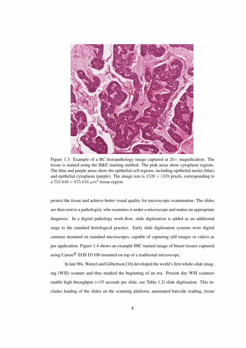
Figure 1.3: Example of a BC histopathology image captured at 20× magnification: Thetissue is stained using the H&E staining method. The pink areas show cytoplasm regions.The blue and purple areas show the epithelial cell regions, including epithelial nuclei (blue)and epithelial cytoplasm (purple). The image size is 1539× 1376 pixels, corresponding toa 755.649× 675.616 µm2 tissue region.

protect the tissue and achieve better visual quality for microscopic examination. The slides

are then sent to a pathologist, who examines it under a microscope and makes an appropriate

diagnosis. In a digital pathology work-flow, slide digitisation is added as an additional

stage to the standard histological practice. Early slide digitisation systems were digital

cameras mounted on standard microscopes, capable of capturing still images or videos as

per application. Figure 1.4 shows an example IHC stained image of breast tissues captured

using Canon R© EOS D1100 mounted on top of a traditional microscope.

In late 90s, Watzel and Gilbertson [16] developed the world’s first whole-slide imag-

ing (WSI) scanner and thus marked the beginning of an era. Present day WSI scanners

enable high throughput (≈35 seconds per slide, see Table 1.2) slide digitisation. This in-

cludes loading of the slides on the scanning platform, automated barcode reading, tissue

8

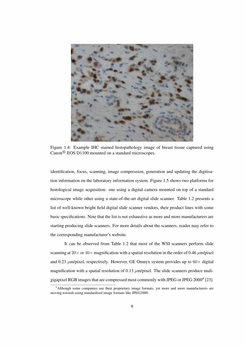
Figure 1.4: Example IHC stained histopathology image of breast tissue captured usingCanon R© EOS D1100 mounted on a standard microscopes.

identification, focus, scanning, image compression, generation and updating the digitisa-

tion information on the laboratory information system. Figure 1.5 shows two platforms for

histological image acquisition: one using a digital camera mounted on top of a standard

microscope while other using a state-of-the-art digital slide scanner. Table 1.2 presents a

list of well-known bright field digital slide scanner vendors, their product lines with some

basic specifications. Note that the list is not exhaustive as more and more manufacturers are

starting producing slide scanners. For more details about the scanners, reader may refer to

the corresponding manufacturer’s website.

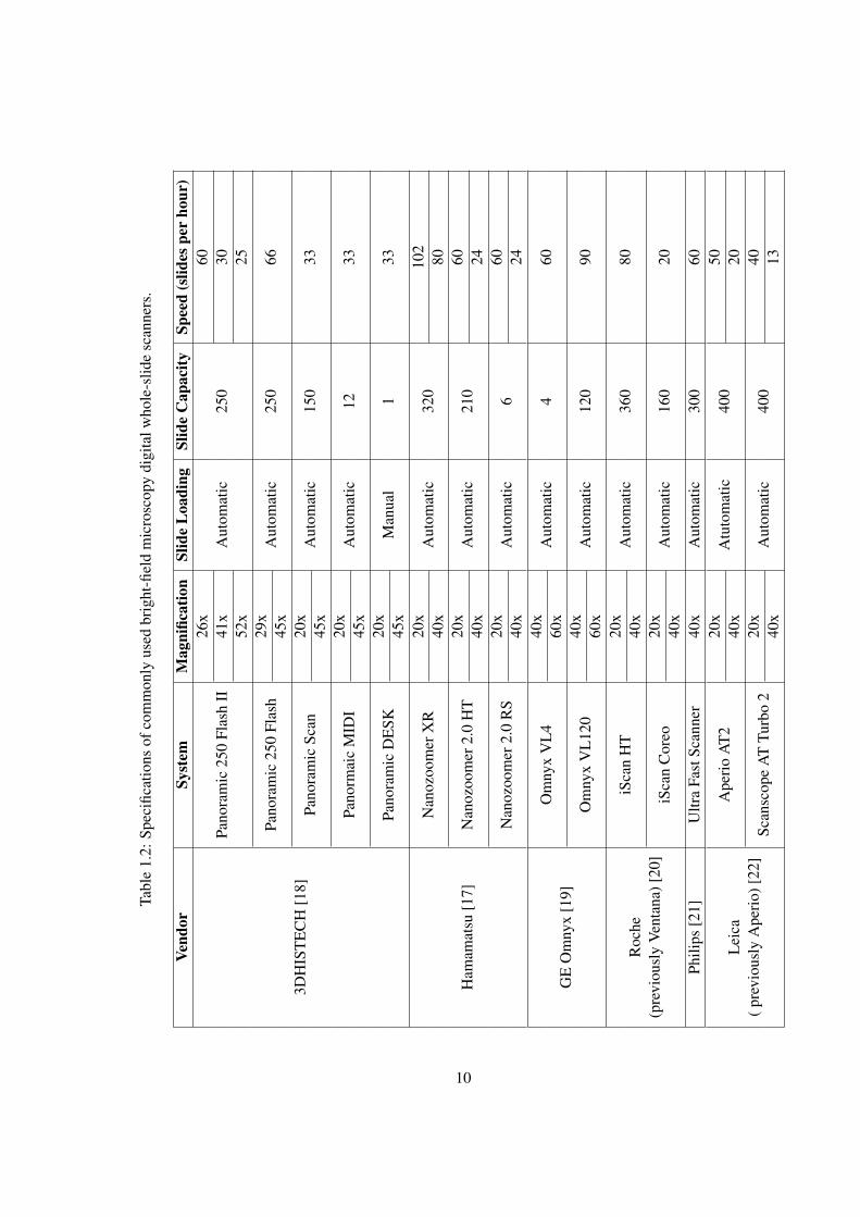
It can be observed from Table 1.2 that most of the WSI scanners perform slide

scanning at 20× or 40×magnification with a spatial resolution in the order of 0.46 µm/pixel

and 0.23 µm/pixel, respectively. However, GE Omnyx system provides up to 60× digital

magnification with a spatial resolution of 0.13 µm/pixel. The slide scanners produce muli-

gigapixel RGB images that are compressed most commonly with JPEG or JPEG 20004 [23].4Although some companies use their proprietary image formats, yet more and more manufacturers are

moving towards using standardised image formats like JPEG2000.

9

Tabl

e1.

2:Sp

ecifi

catio

nsof

com

mon

lyus

edbr

ight

-fiel

dm

icro

scop

ydi

gita

lwho

le-s

lide

scan

ners

.

Vend

orSy

stem

Mag

nific

atio

nSl

ide

Loa

ding

Slid

eC

apac

itySp

eed

(slid

espe

rho

ur)

3DH

IST

EC

H[1

8]

Pano

ram

ic25

0Fl

ash

II26

xA

utom

atic

250

6041

x30

52x

25

Pano

ram

ic25

0Fl

ash

29x

Aut

omat

ic25

066

45x

Pano

ram

icSc

an20

xA

utom

atic

150

3345

x

Pano

rmai

cM

IDI

20x

Aut

omat

ic12

3345

x

Pano

ram

icD

ESK

20x

Man

ual

133

45x

Ham

amat

su[1

7]

Nan

ozoo

mer

XR

20x

Aut

omat

ic32

010

240

x80

Nan

ozoo

mer

2.0

HT

20x

Aut

omat

ic21

060

40x

24

Nan

ozoo

mer

2.0

RS

20x

Aut

omat

ic6

6040

x24

GE

Om

nyx

[19]

Om

nyx

VL

440

xA

utom

atic

460

60x

Om

nyx

VL

120

40x

Aut

omat

ic12

090

60x

Roc

he(p

revi

ousl

yV

enta

na)[

20]

iSca

nH

T20

xA

utom

atic

360

8040

x

iSca

nC

oreo

20x

Aut

omat

ic16

020

40x

Phili

ps[2

1]U

ltra

Fast

Scan

ner

40x

Aut

omat

ic30

060

Lei

ca(p

revi

ousl

yA

peri

o)[2

2]

Ape

rio

AT

220

xA

tuto

mat

ic40

050

40x

20

Scan

scop

eA

TTu

rbo

220

xA

utom

atic

400

4040

x13

10

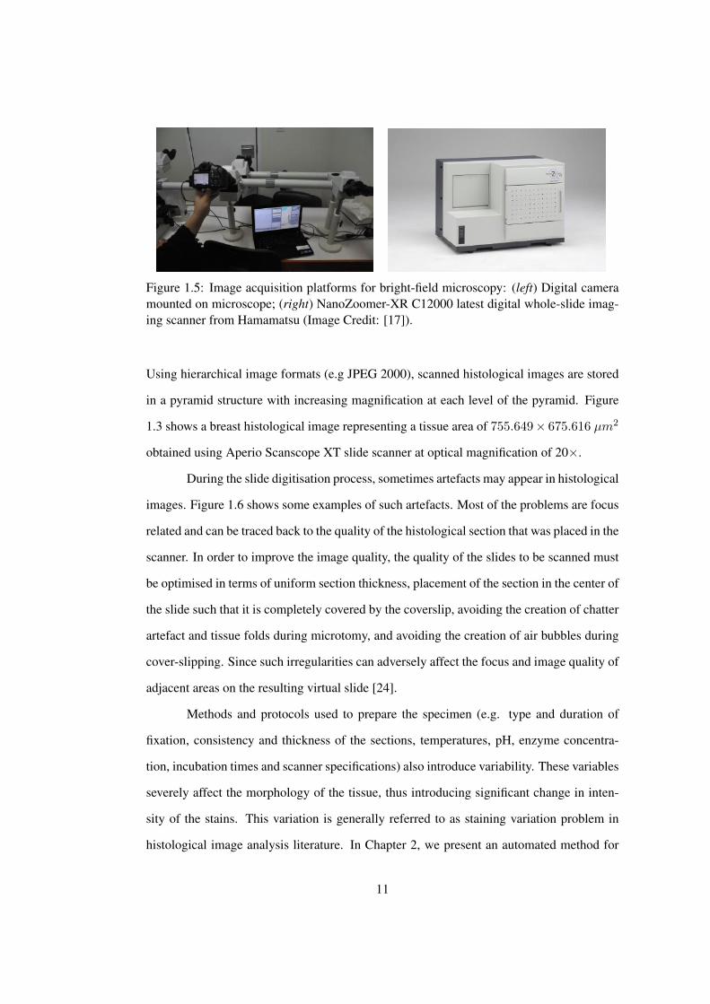
Figure 1.5: Image acquisition platforms for bright-field microscopy: (left) Digital cameramounted on microscope; (right) NanoZoomer-XR C12000 latest digital whole-slide imag-ing scanner from Hamamatsu (Image Credit: [17]).

Using hierarchical image formats (e.g JPEG 2000), scanned histological images are stored

in a pyramid structure with increasing magnification at each level of the pyramid. Figure

1.3 shows a breast histological image representing a tissue area of 755.649× 675.616 µm2

obtained using Aperio Scanscope XT slide scanner at optical magnification of 20×.

During the slide digitisation process, sometimes artefacts may appear in histological

images. Figure 1.6 shows some examples of such artefacts. Most of the problems are focus

related and can be traced back to the quality of the histological section that was placed in the

scanner. In order to improve the image quality, the quality of the slides to be scanned must

be optimised in terms of uniform section thickness, placement of the section in the center of

the slide such that it is completely covered by the coverslip, avoiding the creation of chatter

artefact and tissue folds during microtomy, and avoiding the creation of air bubbles during

cover-slipping. Since such irregularities can adversely affect the focus and image quality of

adjacent areas on the resulting virtual slide [24].

Methods and protocols used to prepare the specimen (e.g. type and duration of

fixation, consistency and thickness of the sections, temperatures, pH, enzyme concentra-

tion, incubation times and scanner specifications) also introduce variability. These variables

severely affect the morphology of the tissue, thus introducing significant change in inten-

sity of the stains. This variation is generally referred to as staining variation problem in

histological image analysis literature. In Chapter 2, we present an automated method for

11

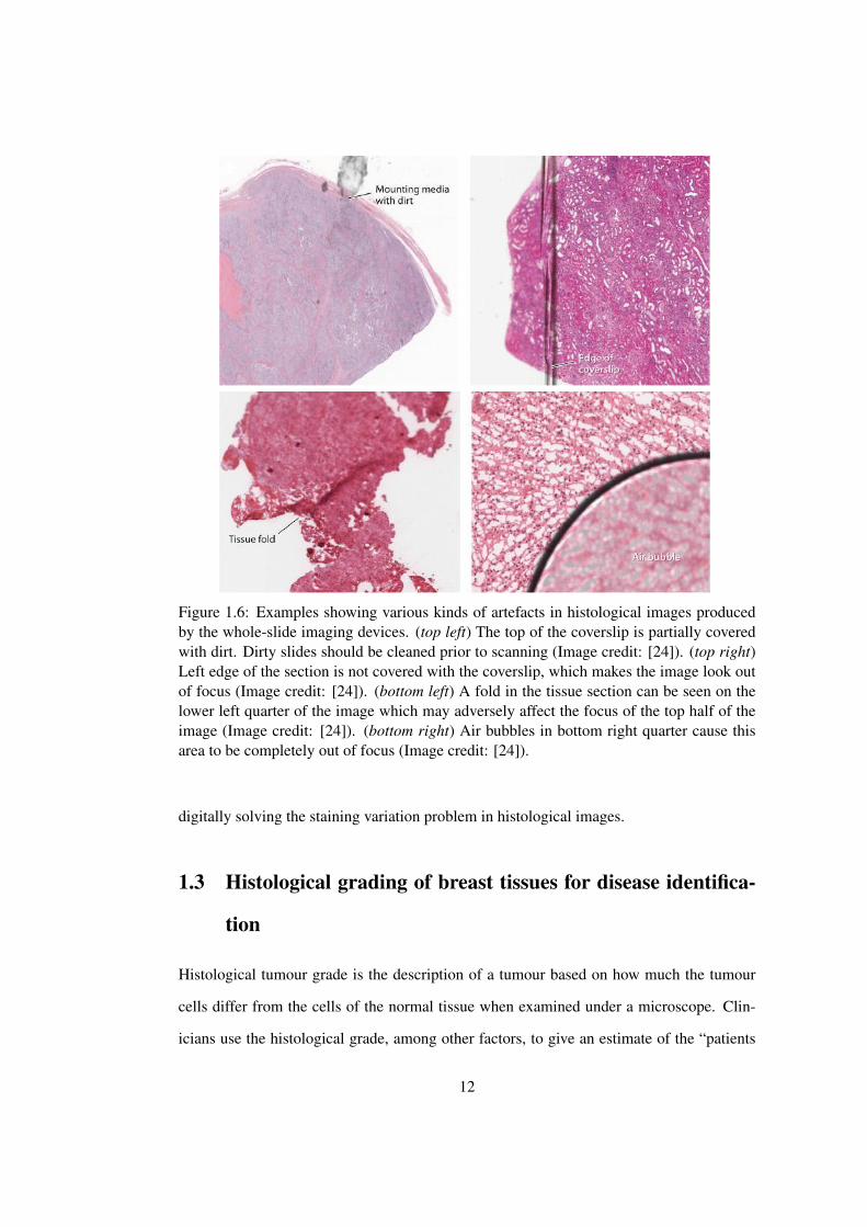
Figure 1.6: Examples showing various kinds of artefacts in histological images producedby the whole-slide imaging devices. (top left) The top of the coverslip is partially coveredwith dirt. Dirty slides should be cleaned prior to scanning (Image credit: [24]). (top right)Left edge of the section is not covered with the coverslip, which makes the image look outof focus (Image credit: [24]). (bottom left) A fold in the tissue section can be seen on thelower left quarter of the image which may adversely affect the focus of the top half of theimage (Image credit: [24]). (bottom right) Air bubbles in bottom right quarter cause thisarea to be completely out of focus (Image credit: [24]).

digitally solving the staining variation problem in histological images.

1.3 Histological grading of breast tissues for disease identifica-

tion

Histological tumour grade is the description of a tumour based on how much the tumour

cells differ from the cells of the normal tissue when examined under a microscope. Clin-

icians use the histological grade, among other factors, to give an estimate of the “patients

12

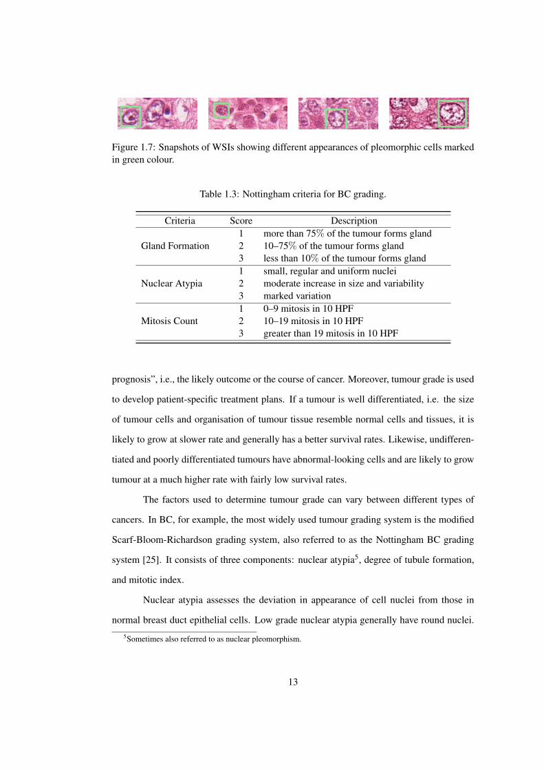
Figure 1.7: Snapshots of WSIs showing different appearances of pleomorphic cells markedin green colour.

Table 1.3: Nottingham criteria for BC grading.

Criteria Score Description

Gland Formation1 more than 75% of the tumour forms gland2 10–75% of the tumour forms gland3 less than 10% of the tumour forms gland

Nuclear Atypia1 small, regular and uniform nuclei2 moderate increase in size and variability3 marked variation

Mitosis Count1 0–9 mitosis in 10 HPF2 10–19 mitosis in 10 HPF3 greater than 19 mitosis in 10 HPF

prognosis”, i.e., the likely outcome or the course of cancer. Moreover, tumour grade is used

to develop patient-specific treatment plans. If a tumour is well differentiated, i.e. the size

of tumour cells and organisation of tumour tissue resemble normal cells and tissues, it is

likely to grow at slower rate and generally has a better survival rates. Likewise, undifferen-

tiated and poorly differentiated tumours have abnormal-looking cells and are likely to grow

tumour at a much higher rate with fairly low survival rates.

The factors used to determine tumour grade can vary between different types of

cancers. In BC, for example, the most widely used tumour grading system is the modified

Scarf-Bloom-Richardson grading system, also referred to as the Nottingham BC grading

system [25]. It consists of three components: nuclear atypia5, degree of tubule formation,

and mitotic index.

Nuclear atypia assesses the deviation in appearance of cell nuclei from those in

normal breast duct epithelial cells. Low grade nuclear atypia generally have round nuclei.5Sometimes also referred to as nuclear pleomorphism.

13

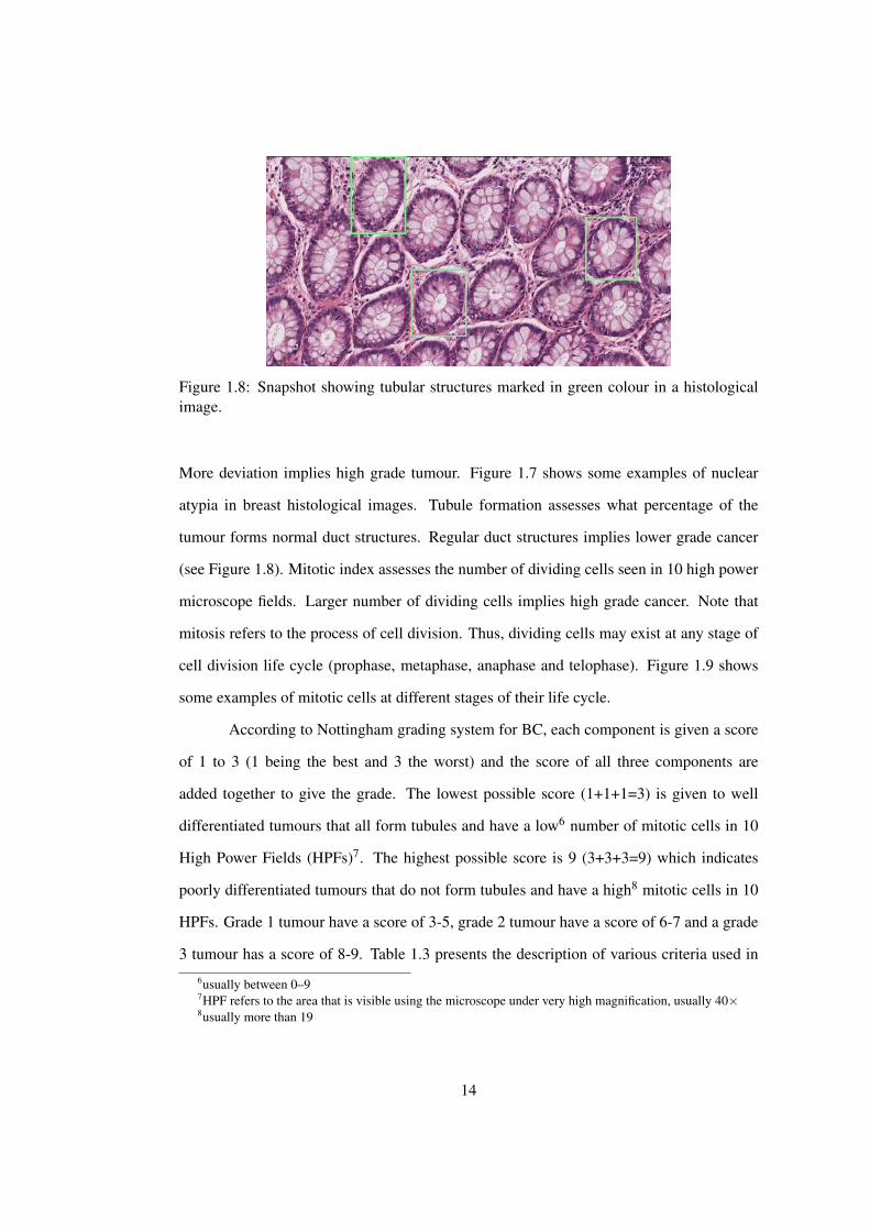
Figure 1.8: Snapshot showing tubular structures marked in green colour in a histologicalimage.

More deviation implies high grade tumour. Figure 1.7 shows some examples of nuclear

atypia in breast histological images. Tubule formation assesses what percentage of the

tumour forms normal duct structures. Regular duct structures implies lower grade cancer

(see Figure 1.8). Mitotic index assesses the number of dividing cells seen in 10 high power

microscope fields. Larger number of dividing cells implies high grade cancer. Note that

mitosis refers to the process of cell division. Thus, dividing cells may exist at any stage of

cell division life cycle (prophase, metaphase, anaphase and telophase). Figure 1.9 shows

some examples of mitotic cells at different stages of their life cycle.

According to Nottingham grading system for BC, each component is given a score

of 1 to 3 (1 being the best and 3 the worst) and the score of all three components are

added together to give the grade. The lowest possible score (1+1+1=3) is given to well

differentiated tumours that all form tubules and have a low6 number of mitotic cells in 10

High Power Fields (HPFs)7. The highest possible score is 9 (3+3+3=9) which indicates

poorly differentiated tumours that do not form tubules and have a high8 mitotic cells in 10

HPFs. Grade 1 tumour have a score of 3-5, grade 2 tumour have a score of 6-7 and a grade

3 tumour has a score of 8-9. Table 1.3 presents the description of various criteria used in6usually between 0–97HPF refers to the area that is visible using the microscope under very high magnification, usually 40×8usually more than 19

14

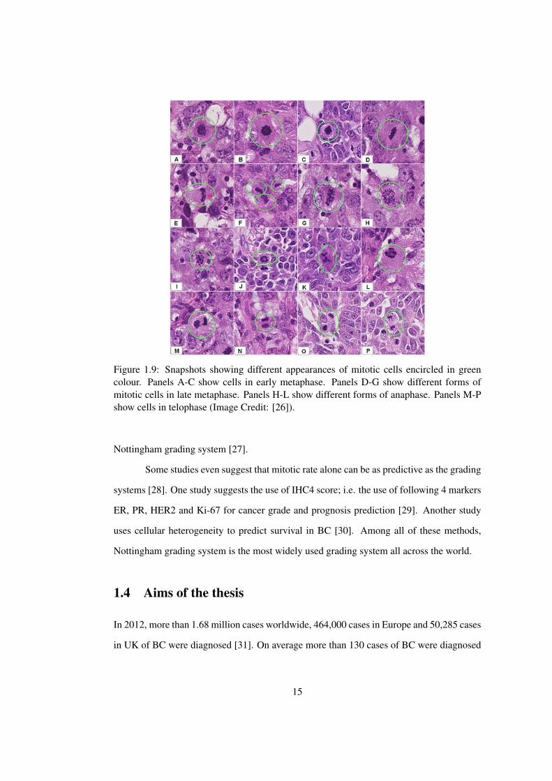
Figure 1.9: Snapshots showing different appearances of mitotic cells encircled in greencolour. Panels A-C show cells in early metaphase. Panels D-G show different forms ofmitotic cells in late metaphase. Panels H-L show different forms of anaphase. Panels M-Pshow cells in telophase (Image Credit: [26]).

Nottingham grading system [27].

Some studies even suggest that mitotic rate alone can be as predictive as the grading

systems [28]. One study suggests the use of IHC4 score; i.e. the use of following 4 markers

ER, PR, HER2 and Ki-67 for cancer grade and prognosis prediction [29]. Another study

uses cellular heterogeneity to predict survival in BC [30]. Among all of these methods,

Nottingham grading system is the most widely used grading system all across the world.

1.4 Aims of the thesis

In 2012, more than 1.68 million cases worldwide, 464,000 cases in Europe and 50,285 cases

in UK of BC were diagnosed [31]. On average more than 130 cases of BC were diagnosed

15

per day in UK alone. From among these, 11,716 (23.29%) patients lost their lives. Although

survival rates have improved by 40% as compared to the figures in mid-80s, there is still a

big margin for improvement part of which can be accomplished by removing subjectivity

from the the diagnostic process.

While Nottingham grading system is the most commonly used grading system for

BC, it often suffers from inter-observer and even intra-observer variability due to its inherent

subjective nature potentially affecting patient prognosis and also the treatment modalities

offered. In one study, for example, a group of 6 pathologists given standardised criteria

agreed on tumour grade in only 58% of cases [32]. In another more recent study on ran-

dom and systematic errors in BC grading, a significant inter-observer disagreement (41.6%)

in classification of grades was observed between two experienced pathologists [33]. The

most frequent disagreement was observed between grade-2 a and grade-3 BC. Overall, al-

most 50% of disagreements were found to be clinically relevant that would imply different

treatment strategies [33].

This variability in BC grading may, at least in part, be responsible for the variabil-

ity in rates of chemotherapy use between institutions. With the advent of digital imaging

in pathology, which has enabled cost and time efficient digitisation of whole histological

slides, automatic image analysis can be suggested as a way to tackle these problems in an

efficient and reliable manner [34].

Computerised analysis of digitised histological images promises to bring objectiv-

ity and reproducibility using image analysis techniques and has the potential to provide

micro and macro prognostic cues, which may be ignored during the visual examination

by humans. For instance, Beck et al. [35] developed a system that predicts the BC grade

based on features calculated from the stromal regions of the tissue, unlike the conventional

Nottingham grading system, where cancer grading is performed based on nuclear atypia,

glandular structures and mitotic index. This happened because of utilisation of immense

computational resources of today’s computers that can learn complex relationships in data

even in unsupervised settings [36]. Thus, we can develop quantitative image analysis tools

16

that can improve the diagnostic and prognostic efficiency of the pathological work-flow, and

at the same time may help us improve our understanding of various biological mechanisms

related to disease progression.

One of the generic problems in histological image analysis is the colour variation in

tissue appearance due to variation in tissue preparation process, stain reactivity from differ-

ent manufacturers/batches, user or protocol variation and the use of scanners from different

manufacturers. We introduce a novel algorithm for stain normalisation in histopathology

images that is based on non-linear mapping of staining characteristics from a source image

to a target image using a representation derived from colour deconvolution (CD). CD is

a method to obtain stain concentration values when the stain matrix, describing how the

colour is affected by the stain concentration, is given. Rather than relying on standard stain

matrices, which may be inappropriate for a given image, a colour based classifier is pro-

posed, that incorporates a novel stain colour descriptor (SCD) to calculate image-specific

stain matrix.

Another common and challenging task in histological image analysis is to highlight

tumour regions in histological images so as to restrict the automated analysis to tumour

regions only and avoid potentially noisy measurements from non-tumour regions. It is

also useful for other tasks related to BC grading such as automated scoring of IHC stained

slides and detection of mitotic cells. We propose an algorithm for unsupervised tumour

segmentation in BC histopathology images. The novelty of the proposed approach lies in

casting the dual problem of segmenting two main types of stromal regions: hypo-cellular

stroma (HypoCS) and hyper-cellular stroma (HyperCS) and employing a hybrid of features

derived from magnitude and phase spectra of the frequency domain to perform accurate

segmentation of tumour areas in BC histopathology images.

Detection, segmentation and quantification of any particular type of nuclei is one of

the most challenging tasks in histological image analysis. Some reasons for this difficulty

are: (1) there are different kinds of nuclei in histological images such as normal, cancerous,

mitotic, apoptotic, lymphocytes etc. and their morphometric attributes overlap significantly;

17

(2) staining variation as discussed above; (3) variations in appearance due to sectioning pro-

cess9. We develop a framework for detection of mitotic cells in BC histopathology images,

which as explained in Section 1.3, is crucial for realisation of an automated BC grading sys-

tem. The proposed algorithm models the pixel intensities in mitotic and non-mitotic regions

by a Gamma-Gaussian mixture model [37] (GGMM) and employs a discriminative dictio-

nary learning approach to model the visual appearance of mitotic cells and non-mitotic cells

along with the immediate surrounding context [38].

Automatic nuclear atypia scoring is crucial for the development of an automated

BC grading system using the Nottingham grading system approach. We propose an im-

age level descriptor that efficiently performs nuclear atypia scoring in BC histopathology

images. The image level descriptor is obtained using an affine-invariant geodesic mean of

region covariance (RC) descriptors [39] on the Riemannian manifold of symmetric posi-

tive definite (SPD) matrices [40]. The resulting image descriptors are also SPD matrices,

lending themselves to tractable geodesic distance based k-nearest neighbour (kNN) classi-

fication using efficient kernels.

1.5 Thesis organisation

This thesis is organised into six chapters. Following a brief introduction of the area of histo-

logical images analysis in Chapter 1, we introduce an algorithm in Chapter 2 that automat-

ically normalise the colour variation in histological images, such that the stain normalised

histological images demonstrate a consistent absorption of histological stains across dif-

ferent tissue specimen. Chapter 3 presents an algorithm for tumour segmentation in BC

histopathology images which play an important role in improving the accuracy of mitotic

cell detection framework in Chapter 4. Chapter 5 presents a framework for nuclear atypia

scoring in BC histopathology images. In Chapter 6, we summarise the main contributions

of this thesis and present some possible directions for future research.9see Chapter 4 for a detailed discussion on this topic

18

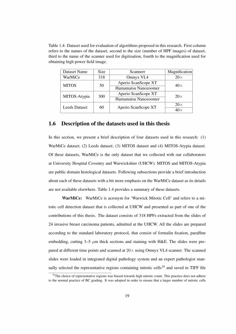
Table 1.4: Dataset used for evaluation of algorithms proposed in this research. First columnrefers to the names of the dataset, second to the size (number of HPF images) of dataset,third to the name of the scanner used for digitisation, fourth to the magnification used forobtaining high power field image.

Dataset Name Size Scannerr MagnificationWarMiCe 318 Omnyx VL4 20×MITOS 50

Aperio ScanScope XT40×

Hamamatsu Nanozoomer

MITOS-Atypia 300Aperio ScanScope XT

20×Hamamatsu Nanozoomer

Leeds Dataset 60 Aperio ScanScope XT20×40×

1.6 Description of the datasets used in this thesis

In this section, we present a brief description of four datasets used in this research: (1)

WarMiCe dataset; (2) Leeds dataset; (3) MITOS dataset and (4) MITOS-Atypia dataset.

Of these datasets, WarMiCe is the only dataset that we collected with our collaborators

at University Hospital Coventry and Warwickshire (UHCW). MITOS and MITOS-Atypia

are public domain histological datasets. Following subsections provide a brief introduction

about each of these datasets with a bit more emphasis on the WarMiCe dataset as its details

are not available elsewhere. Table 1.4 provides a summary of these datasets.

WarMiCe: WarMiCe is acronym for ‘Warwick Mitotic Cell’ and refers to a mi-

totic cell detection dataset that is collected at UHCW and presented as part of one of the

contributions of this thesis. The dataset consists of 318 HPFs extracted from the slides of

24 invasive breast carcinoma patients, admitted at the UHCW. All the slides are prepared

according to the standard laboratory protocol, that consist of formalin fixation, paraffine

embedding, cutting 3–5 µm thick sections and staining with H&E. The slides were pre-

pared at different time points and scanned at 20× using Omnyx VL4 scanner. The scanned

slides were loaded in integrated digital pathology system and an expert pathologist man-

ually selected the representative regions containing mitotic cells10 and saved in TIFF file10The choice of representative regions was biased towards high mitotic count. This practice does not adhere

to the normal practice of BC grading. It was adopted in order to ensure that a larger number of mitotic cells

19

format at digital magnification of 40×. A total of 318 HPFs were generated each of size

1920× 1153 pixels.

The ground truth (GT) marking for mitotic cells was performed based on annota-

tions by multiple expert pathologists, to reduce the inter-observer variability. Three expert

pathologists independently marked the HPFs by drawing a circle around the mitotic cells.

It is worth emphasising that the pathologists marked the mitotic cells on a computer screen

as compared to microscopes, where they are generally trained to work on. The process

of GT marking was blind as all three experts performed GT marking independent of each

other. The objects on which all three pathologists agreed were directly accepted as GT

mitotic cells. The conflicting objects (marked as mitotic cells by at least one of the pathol-

ogists) were presented to the panel of three pathologists to make the final decision. The

panel comprised of the same three pathologists, who marked the slides in the first instance.

The only difference was that this time the three experts were sitting in a single room and

going through each conflicting cell concurrently, and after discussion either selecting the

cell as GT or discarding it. The total number of cells after the consensus annotation were

1267. Note that these include the initial mutually agreed cells as well, on which all three

pathologists agreed as mitosis. We make use of WarMiCe dataset for performing mitotic

cell detection experiments in Chapter 4.

Leeds Dataset:

The dataset consists of 5 batches of 12 images each (60 images, ≈ 0.5 Million

pixels manually labelled as one of the two classes: stained (Hematoxylin, Eosin, Dab)

or background). Four batches contain liver tissues, with the fifth containing oesophageal

tissue. These batches were prepared at different times using different chemical batches by

a range of technicians within Leeds Hospital laboratories. All tissues are formalin fixed,

paraffin embedded, H&E counterstained. Virtual slides were obtained by scanning glass

slides at 50,000 or 100,000 dpi (20× or 40× magnification) using the Aperio XT scanner.

Representative images (typically 1, 000 × 1, 000) at native resolution were extracted from

could be identified. This would result in dataset of a size that is sufficient for training and evaluation of anautomatic mitotic cell detection algorithm.

20

the WSIs and saved as JPEG images (JPEG quality=100%). The Leed dataset is utilised

during stain normalisation experiments in Chapter 2.

MITOS: MITOS11 is a publicly available dataset for detection of mitosis in BC

histopathology images [41]. The dataset consists of 50 HPFs acquired from the breast

tissues slides of 5 different patients. Each slide is stained with H&E. Each HPF represents

a 512 × 512µm2 area, and is acquired using three different equipment setups: two slide

scanners and a multispectral microscope. In this research, we only use the images obtained

from the two slide scanners: Aperio XT and Hamamatsu. Aperio HPFs have a resolution of

0.2456µm per pixel, resulting in a 2, 084×2, 084 RGB image, while the Hamamatsu HPFs

have a horizontal and vertical resolution of 0.2273 and 0.22753µm per pixel, resulting in

a 2, 252 × 2, 250 RGB image. Three expert pathologists manually annotated the slides for

mitotic cells by first identifying them on microscopes and then verifying them on digital

slide visualisation platform. There are in total 326 mitotic cells in the MITOS dataset. We

make use of MITOS dataset for performing stain normalisation experiments in Chapter 2,

tumour segmentation experiments in Chapter 3 and mitotic cell detection experiments in

Chapter 4.

MITOS-ATYPIA: MITOS-Atypia12 is an extension of the publicly available MI-

TOS dataset [41]. The dataset is part of an ongoing contest on nuclear atypia scoring in

BC histopathology images. It consists of H&E stained slides obtained from 11 patients,

scanned using two different scanners: Aperio Scanscope XT and Hamamatsu Nanozoomer

HT. From the tumour regions of all the BC biopsy slides, a total of 300 frames are extracted

at 20× magnification. Each frame is independently scored for nuclear atypia by two expert

pathologists. The score assigned to each frame is a discrete number between 1 and 3. Score

1 represents the low grade nuclear atypia and Score 3 the high grade nuclear atypia. In

approximately 15% of the cases, the two experts disagreed. For these conflicting cases, a

third pathologist scored the slides independently and majority vote was used as the final

nuclear atypia score. We make use of MITOS-Atypia dataset for performing nuclear atypia11http://ipal.cnrs.fr/ICPR2012/?q=node/512http://mitos-atypia-14.grand-challenge.org/

21

scoring experiments in Chapter 5.

1.7 Summary

This chapter presented a brief introduction to the digital histopathology work-flow that

involves tissue specimen extraction, preparation for histological analysis and digitisation.

After digitisation, a whole-slide tissue specimen is converted to a histological image and can

be readily analysed using quantitative image analysis techniques which promise to provide

more objectivity and reproducibility in histological analysis. The main focus of this thesis

is on developing computerised image analysis algorithms for histological analysis. We

develop a generic histological image analysis algorithm for stain normalisation and three

algorithms related specifically to BC tissues: tumour segmentation, mitotic cell detection

and nuclear atypia scoring. Stain normalisation has high significance in the domain of

histological image analysis while mitotic cell detection and nuclear atypia scoring have

high diagnostic and prognostic significance in BC grading.

22

Chapter 2

Stain Normalisation

2.1 Introduction

Histopathology is the diagnosis of disease by visual examination of tissue under the micro-

scope. In order to examine tissue sections (which are virtually transparent), tissue sections

are prepared using coloured histochemical stains that bind selectively to cellular compo-

nents. Colour variation is a problem in histopathology based on light microscopy due to a

range of factors such as the use of different scanners, variable chemical colouring/reactivity

from different manufacturers/batches of stains, colouring being dependent on staining pro-

cedure (timing, concentrations etc.), and light transmission being a function of section

thickness (see Figure 2.1and 2.2). Lyon et al. [42] outline the need for standardisation

of reagents and procedures in histological practice. However, because of issues like manual

sectioning variability and stains fading over time, complete standardisation is not possible

to achieve with the current technology. Current practice is limited to physical and proce-

dural quality control methods, including subjective assessment of stain quality and inter-

laboratory comparisons of staining, in order to minimise the visible variability in staining

and its impact on diagnostic quality.

With the advent of digital imaging and automatic image analysis, colour variation

in histopathology has become more of an issue. For example, many commercial image

24

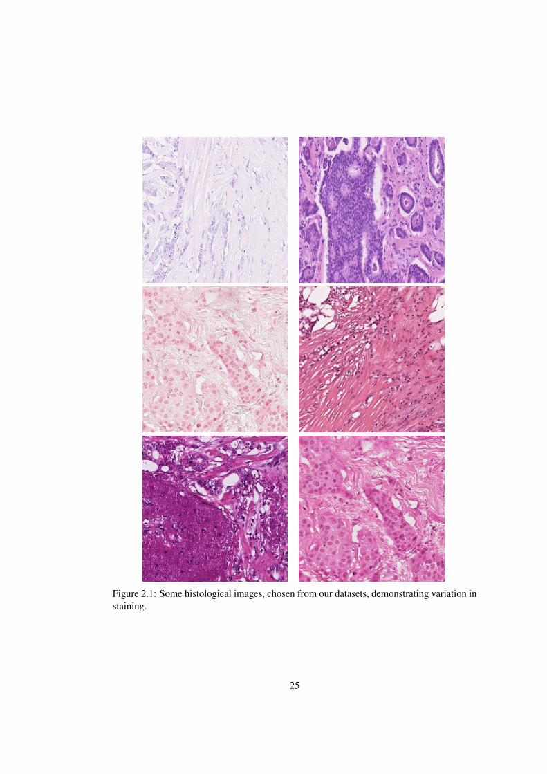
Figure 2.1: Some histological images, chosen from our datasets, demonstrating variation instaining.

25

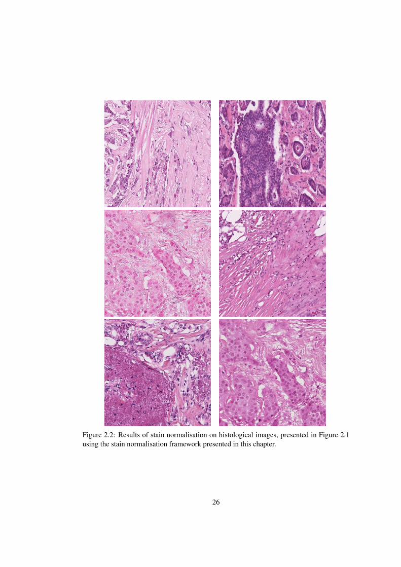
Figure 2.2: Results of stain normalisation on histological images, presented in Figure 2.1using the stain normalisation framework presented in this chapter.

26

analysis algorithms require parameters defining the expected colour of anatomy of inter-

est and fail if these parameters are incorrect. Although methods have been proposed for

improving colour constancy in images formed via Lambertian (reflective) model of image

formation (see [43] for a good overview), these methods are not applicable to colour im-

ages formed via light transmission through a tissue specimen, and thus are inappropriate for

histopathology image analysis.

Consequently, a large number of methods presented in the area of automatic image

analysis of colour histopathology images bypass the problem of colour constancy by trans-

forming the images to greyscale. For example, texture analysis for tissue type classification

has been performed on greyscale images using features based on greyscale co-occurrence

matrices [44, 45], local binary patterns (LBP) [46, 47], or the wavelet packet transform [48].

This can be successful in cases where greyscale intensity is the primary cue. For example,

Basavanhally et al. [49] use the fact that cell nuclei are much darker under certain stains

than surrounding anatomy. Luminance is used to classify different types of nuclei in their

work. However, conversion to greyscale ignores the wealth of information in the colour

representation used routinely by the pathologists. Typically, 2 or 3 different coloured stains

are used to highlight the cellular and subcellular target components. The intensity of each

colour is related to the concentration of the corresponding component. Additionally, more

than one target component protein may be present in a given area, resulting in a mix of

colour. Converting images to greyscale results in an image representing the total concen-

tration of all tissue components, rather than the relative amounts of each.

Some authors have included colour information within texture based image classifi-

cation in digital histopathology image analysis [50, 51]. Kong et al. [52] use co-occurrence

matrices in individual channels of the Lab colour space as texture descriptor, and evaluate a

range of different classifiers for grading neuroblastic differentiation. Sertel et al. [53] clus-

ter colour vectors in the Lab colour space using k-means clustering and use a co-occurrence

representation based on colour prototypes as a texture feature. Considering the variation in

colours within/across histopathology sections, colour texture features may be highly sensi-

27

tive to staining/scanner variations which can then significantly affect the performance of an

automated or computer-assisted diagnostic.

In order to overcome these limitations, there are two solutions proposed in the lit-

erature: (1) implicit standardisation of stains by developing algorithms that are robust to

variation in staining [54, 55]. This generally involves dynamically estimating the colour

distribution of each individual image from a set of salient objects, where salient objects

depend on the problem domain (e.g. nuclei as in the case of [54, 55]); (2) explicit stan-

dardisation of stains by developing algorithms that can be adopted as preprocessing steps

in histological image analysis algorithms [56, 57, 58, 59, 60, 61, 62, 63, 64]. Among these

standardisation approaches, explicit standardisation is more widely adopted.

In histopathology image analysis, Wang et al. [65] were the first to use explicit

standardisation. They proposed a framework, where they normalise colour distributions of

source image to those of a target image before performing colour-based segmentation. In

the remainder of this chapter, we use the term stain or colour normalisation to refer to the

process of adjusting the colour values of an image on a pixel-by-pixel basis so as to match

the colour distribution of the source image to that of a target image.

In the existing literature, several stain normalisation methods can be found [56,

57, 58, 59, 60, 61, 62, 63, 66, 67, 68, 69, 70]. Histogram specification [66] is a method

closely related to histogram equalisation previously used for colour normalisation in oral

histopathology images [71] and retinal images [72]. A major drawback of histogram based

approaches is that they introduce considerable visual artifacts in images. This is due to the

implicit assumption that the proportion of pixels of each stain type is same in the target

and source images. This is clearly not always the case (see Figure 2.3). Kothari et al. [56]

proposed a variation on histogram normalisation where the presence of a colour rather than

frequency is used for colour normalisation. This has the disadvantage that rare (potentially

noise), and common pixel values are treated as equally important.

Reinhard et al. [57] proposed a method of colour normalisation where the mean

and standard deviation of each channel of the image are matched to that of the target by

28

means of a set of linear transforms in the Lab colour space. However, the assumption of

unimodal distribution of pixels in each channel of the Lab colour space does not hold if

multiple coloured stains are used. As a result, this can result in background areas being

mapped as coloured regions, and foreground being incorrectly mapped, as shown in Figure

2.3. Magee et al. [58] proposed an automatic segmentation extension to [57]. First, Gaus-

sian mixture model (GMM) based colour segmentation is used to automatically identify

multiple pixel classes, then linear normalisation is applied separately to each pixel class,

where class membership is defined by a pixel being coloured by a particular chemical stain,

or background. A major limitation of this approach is that it introduces artifacts near pixels

that lie on the class boundary.

Basavanhally et al. [62] proposed a colour normalisation approach that combines

the two approaches, Reinhard and histogram equalisation, by performing unsupervised seg-

mentation of a tissue into four components (nuclei, stroma, epithelium and background),

and mapping of RGB histograms of each component to the histogram of corresponding

component in a template (reference) image.

CD [73, 74] is used extensively in histopathology image analysis for decomposition

of an RGB image into stain channels, where each stain channel corresponds to the actual

colours of the stain used (see Section 2.2 for details). Although [73] is the the most widely

used framework for CD, its accuracy depends heavily on the accurate definition of absorp-

tion spectra for each stain to be separated, also referred to as stain matrix in the following

text. More recently, Gavrilovic et al. [74] have proposed a blind CD framework that does

not require prior definition of stain matrix.

Magee et al. [58] and Macenko et al. [59] simultaneously proposed methods for

stain normalisation based on a CD derived representation. Both methods automatically de-

rive image specific CD matrices. Magee et al. use a supervised pixel classification based

approach to estimate stain colours, whereas Macenko et al. use an Singular value decom-

position (SVD) based approach to directly estimate the matrices. Niethammer et al. [60]

extend the stain matrix estimation method in [59] using priors to estimate stain matrices

29

to improve stability in cases where images contain uneven proportions of each stain, at the

cost of abandoning the closed form solution in the original work - thus introducing an ad-

ditional local optima failure mode. Macenko et al. use linear per-channel normalisation

based on a pseudo-maximum (the 99th percentile) to map source image values to match the

target image, whereas Magee et al. use a non-linear mapping based on pixel classifications.

Either method can fail if the stain matrix estimation process fails, the mapping function is

inappropriate, or the channel statistics calculations are inaccurate due to excessive noise

(e.g. saturated pixels). It can be argued that linear normalisation is always inappropriate

as it treats optically and chemically saturated pixels identically to other pixels, modifying

their values (see Figure 2.3). Additionally, Macenko et al. modifies the colour distribution

of both source and target images, which is sometimes not desirable if we have a reference

image with stain characteristics suitable for an automated system.

Stain normalisation approach presented in [61] is also based on stain decomposition

framework, similar to the one presented in [73]. Instead of closed form solution in [73],

they propose to use non-negative matrix factorisation framework to decompose an RGB

image into its constituent stain channels. Moreover, they propose to adjust the contrast

of individual stains channels using Gamma correction, instead of channel mapping in CD

space [64].

Bautista et al. [63] perform colour normalisation using a colour calibration ap-

proach, where a reference slide with known colour characteristics is scanned with the digital

scanner and resultant variation in the true colours and scanned colours is used to correct the

colour variation of histological images. A major limitation of this approach is that it only

takes into account the variation in colours that arise because of scanner variation from dif-

ferent manufacturers or same manufacturer but with different scanning characteristics. It

does not take into account other factors like thickness of tissue sections, concentration of

dyes and staining timings etc., which as explained above are very important considerations

as well.

The stain normalisation approach presented in [69, 70] employs a two step ap-

30

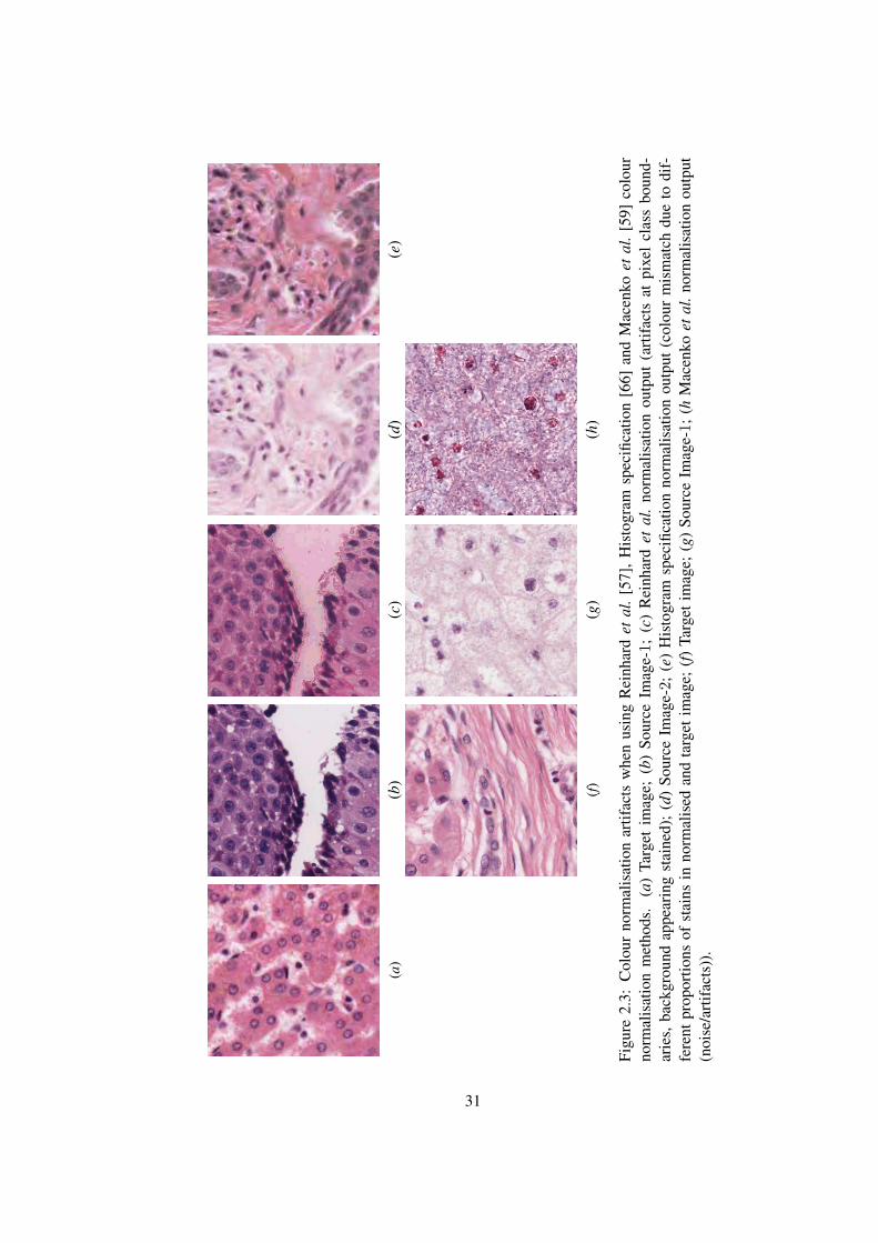
(a)

(b)

(c)

(d)

(e)

(f)

(g)

(h)

Figu

re2.

3:C

olou

rno

rmal

isat

ion

artif

acts

whe

nus

ing

Rei

nhar

det

al.[

57],

His

togr

amsp

ecifi

catio

n[6

6]an

dM

acen

koet

al.[

59]

colo

urno

rmal

isat

ion

met

hods

.(a

)Ta

rget

imag

e;(b

)So

urce

Imag

e-1;

(c)

Rei

nhar

det

al.

norm

alis

atio

nou

tput

(art

ifact

sat

pixe

lcl

ass

boun

d-ar

ies,

back

grou

ndap

pear

ing

stai

ned)

;(d

)So

urce

Imag

e-2;

(e)

His

togr

amsp

ecifi

catio

nno

rmal

isat

ion

outp

ut(c

olou

rm

ism

atch

due

todi

f-fe

rent

prop

ortio

nsof

stai

nsin

norm

alis

edan

dta

rget

imag

e;(f

)Ta

rget

imag

e;(g

)So

urce

Imag

e-1

;(h

Mac

enko

etal

.nor

mal

isat

ion

outp

ut(n

oise

/art

ifact

s)).

31

proach: (1) estimation of colour distribution; (2) correction of colour distribution. Colour

distribution is estimated by sampling a set of colours from a WSI. Correction is performed

by modifying the colour distribution of a source image such that it fits reasonably well with

the colour distribution of a reference image. The approach is evaluated on Elastica van

Gieson stained whole slide liver biopsy images and no evidence was presented regarding

the usability of this approach on H&E stained images.

The method presented in this chapter is an evolution of [58] and overcomes limi-

tations of previous work by estimating stable stain matrices using an image specific colour

descriptor and a robust colour classification framework based on a variety of training data

for a particular stain. Moreover, we propose a regularised non-linear mapping of stain chan-

nels which ensures smooth colour transformation without introducing visual artifacts. The

following list accounts for our novel contributions:

1. We introduce a novel whole-image SCD that grossly quantifies the concentration of

stains in an image. We demonstrate that pixel classification performance is robust for

a wide variety of images if our SCD descriptor is used along with the R,G,B pixel

information (Section 2.3.1).

2. We propose the use of a colour based classifier to calculate image-specific stain ma-

trices (Section 2.3.1).

3. We perform non-linear mapping of source image channels to the target image chan-

nels using regularised spline based functions estimated from image statistics (Section

2.3.2).

4. We demonstrate that a tumour segmentation algorithm for BC histopathology im-

ages [75] demonstrates stable performance if preceded by a stain normalisation step

especially if data is coming from different scanners (Section 2.4.3).

The rest of this chapter is organised as follows. Section 2.2 outlines the details of

CD model which is essential to our proposed stain normalisation framework. In Section

32

2.3, we propose a novel method for automatic derivation of stain matrices by incorporating

global image-specific stain information with local RGB pixel information in a supervised

classification framework [76]. We use the estimated stain matrix to develop a novel stain

normalisation method that automatically adjusts the RGB colour distribution of a source im-

age to that of a target image. Finally, we demonstrate in Section 2.4 that stain normalisation

can play a critical role in stability of automatic histopathology image analysis algorithms

especially when there is variation in the staining protocol or tissue, or the data comes from

different scanners.

2.2 The Colour Deconvolution Model

In 2001, Ruifrok and Johnston [73] proposed CD framework with potential application

in histopathology image analysis. Since then, this method has been used in a variety of

applications; quantification of IHC stains [4, 15] and nuclei detection [77] to name but a

few. The CD framework transforms the RGB colour space Ψ to a new colour space Ψ

defined by the stains used for staining the tissue section. If image I = (C,Ψ) is defined as

a 2-dimensional (2D) set of pixels C with associated colour space function Ψ assigning red,

green and blue intensities to each pixel, the relationship between colour spaces Ψ and Ψ is

defined by Lambert-Beers law as follows [78],

Ψ = exp(−SΨ) (2.1)

where S is the stain matrix that defines the stain vectors (absorption factors) associated with

each stain used on the tissue.

S =

sr,1 sg,1 sb,1

sr,2 sg,2 sb,2

sr,3 sg,3 sb,3

(2.2)

33

where sr,1, sg,1 and sb,1 denote the pre-defined, normalised red, green and blue values for

s1 channel. Similarly, the second and third rows of S are defined for s2 and s3 channels

respectively. Ruifrok & Johnston [73] provided a closed form solution to the inversion of

(2.1), in which they demonstrated that the intensity of a pixel g ∈ C in the new colour space

Ψ is defined as

Ψ(g) = DΦ(g) (2.3)

where D = S−1 (2.4)

and Φ(g) = − log(Ψ(g)) (2.5)

Here, D is the CD matrix obtained by calculating the inverse of the stain matrix S, Φ is

the so-called optical density (OD) space where a linear combination of stains results in a

linear combination of OD values and Ψ(g) represents the amount of each stain (s1, s2 and

s3) corresponding to the pixel g.

CD framework discussed above requires accurate estimation of S (the stain matrix).

Although [73] provides standard stain matrices for a variety of stain combinations, however

an image-specific stain matrix produce more optimal stain separation.

2.3 Stain Normalisation Algorithm

Figure 2.4 gives an overview of the proposed stain normalisation algorithm that consists

of four modules: stain matrix estimation, CD, non-linear mapping of channel statistics and

reconstruction. Broadly, we first map both target =(C,Ψ) and source X (C,Ψ) images to

a representation =(C, Ψ) and X (C, Ψ), where each channel relates to a separate chemical

stain (see Section 2.2). Next, we apply a non-linear correction (mapping) to normalise each

channel of X separately (based on the statistics calculated from the corresponding channel

of =). Finally, we reconstruct the normalised source image X norm using the normalised

stain channels of X .The following subsections present the details of each of these modules.

34

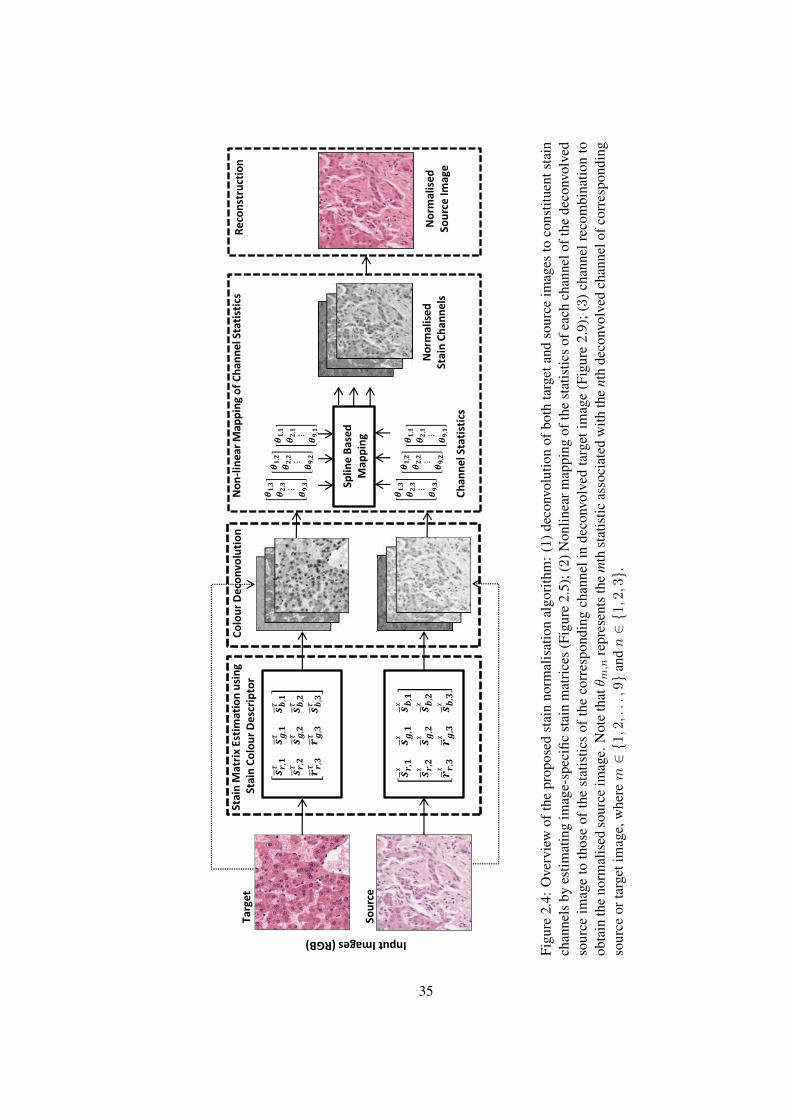
Co

lou

r D

eco

nvo

luti

on

𝒔 𝒓,𝟏

ᵡ 𝒔 𝒈

,𝟏ᵡ

𝒔𝒃,𝟏

ᵡ

𝒔 𝒓,𝟐

ᵡ 𝒔 𝒈

,𝟐ᵡ

𝒔𝒃,𝟐

ᵡ

𝒓𝒓,𝟑

ᵡ 𝒓𝒈,𝟑

ᵡ 𝒔𝒃,𝟑

ᵡ

Stai

n M

atri

x Es

tim

atio

n u

sin

g St

ain

Co

lou

r D

esc

rip

tor

Ch

ann

el S

tati

stic

s

No

rmal

ised

St

ain

Ch

ann

els

𝜽𝟏,𝟑

𝜽𝟐,𝟑 ⋮

𝜽𝟗,𝟑

𝜽𝟏,𝟐

𝜽𝟐,𝟐 ⋮

𝜽𝟗,𝟐

𝜽𝟏,𝟏

𝜽𝟐,𝟏 ⋮

𝜽𝟗,𝟏

𝜽𝟏,𝟑

𝜽𝟐,𝟑 ⋮

𝜽𝟗,𝟑

𝜽𝟏,𝟐

𝜽𝟐,𝟐 ⋮

𝜽𝟗,𝟐

𝜽𝟏,𝟏

𝜽𝟐,𝟏 ⋮

𝜽𝟗,𝟏

No

rmal

ised

So

urc

e Im

age

Input Images (RGB)

𝒔 𝒓,𝟏

𝜏 𝒔𝒈,𝟏

𝜏 𝒔 𝒃

,𝟏𝜏

𝒔 𝒓,𝟐

𝜏 𝒔𝒈,𝟐

𝜏 𝒔 𝒃

,𝟐𝜏

𝒓𝒓,𝟑

𝜏 𝒓𝒈,𝟑

𝜏 𝒔 𝒃

,𝟑𝜏

Splin

e B

ased

M

app

ing

No

n-l

inea

r M

app

ing

of

Ch

ann

el S

tati

stic

sR

eco

nst

ruct

ion

Targ

et

Sou

rce

Figu

re2.

4:O

verv

iew

ofth

epr

opos

edst

ain

norm

alis

atio

nal

gori

thm

:(1

)dec

onvo

lutio

nof

both

targ

etan

dso

urce

imag

esto

cons

titue

ntst

ain

chan

nels

byes

timat

ing

imag

e-sp

ecifi

cst

ain

mat

rice

s(F

igur

e2.

5);(

2)N

onlin

earm

appi

ngof

the

stat

istic

sof

each

chan

nelo

fthe

deco

nvol

ved

sour

ceim

age

toth

ose

ofth

est

atis

tics

ofth

eco

rres

pond

ing

chan

neli

nde

conv

olve

dta

rget

imag

e(F

igur

e2.

9);(

3)

chan

nelr

ecom

bina

tion

toob

tain

the

norm

alis

edso

urce

imag

e.N

ote

thatθ m

,nre

pres

ents

the

mth

stat

istic

asso

ciat

edw

ithth

ent

hde

conv

olve

dch

anne

lofc

orre

spon

ding

sour

ceor

targ

etim

age,

whe

rem∈{1,2,...,9}a

ndn∈{1,2,3}.

35

2.3.1 Stain Matrix Estimation & Colour Deconvolution

We use the CD framework [73] to convert both = and X images from RGB colour space to

a new colour space defined by constituent stains. This requires estimation of image-specific

stain matrix S each for = and X images. We estimate image-specific stain matrices (S=

and SX ) using a global (per-image) SCD and local pixel level colour information in a super-

vised colour classification framework (see following two sub-sections for details). Figure

2.5 gives an overview of the stain matrix estimation method that consists of two phases:

learning and evaluation. Learning, which is performed offline, essentially involves 2 steps:

(1) deriving principal colour histograms (PCH) from a training set of quantised image his-

tograms to obtain SCDs; (2) learning classification models by utilising RGB (pixel informa-

tion) and SCD (whole image colour information) in a supervised classification framework

to generate stain specific probability maps (one for each stain and background). These

probability maps are used to estimate the colour of each stain for a particular image. In the

following subsections, we further elaborate on this method.

Image-Specific Stain Colour Descriptor

Given a training set of k RGB histopathology images I = {I1, I2, . . . , Ik}, we calculate a

set of image associated SCDs H ={H1, H2, . . . , Hk

}. For this purpose, each image Ii

(where i = {1, . . . , k}) is colour quantised using Oct-tree quantisation [79] to generate a set

of histograms of 256 colour prototypesH = {H1, H2, . . . ,Hk}. Oct-tree quantisation [79]

is a very efficient colour to prototype mapping algorithm. The method works by iteratively

partitioning a 3-dimensional (3D) colour space into 8 equal sized regions to form a tree

of regions of increasingly small size. The number of leaves can be reduced by subsuming

multiple leaves of tree by their common parent node (which then becomes a leaf). In our

implementation subsumption is based on the node with the fewest associated pixels until

there are only 256 prototypes.

Next, mean H and covariance Σh of the training set of histograms are computed to

perform linear dimensionality reduction (DR). Let Erh be the matrix whose columns are the

36

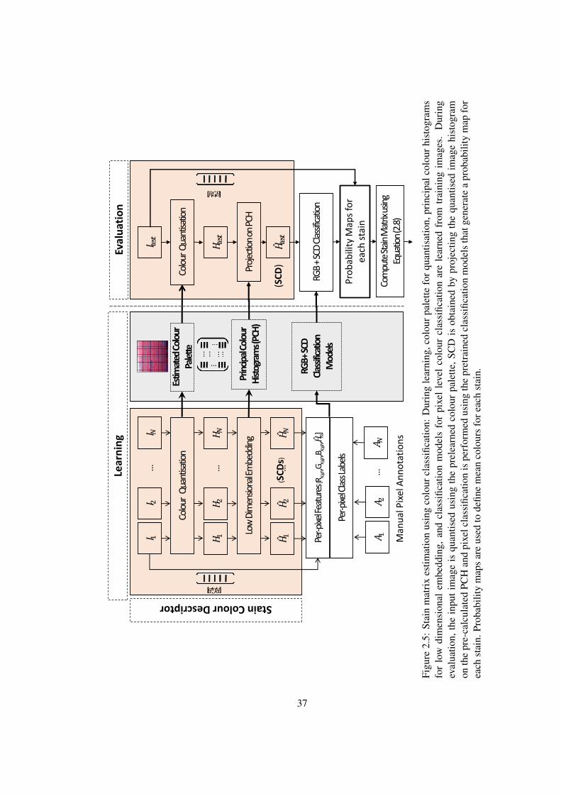
𝐼 1𝐼 2

…𝐼 𝑁

𝐻 1𝐻 2

…𝐻 𝑁

Colo

ur Q

uant

isatio

n

Low

Dim

ensio

nal E

mbe

ddin

g

𝐻 1 𝐻 2

… 𝐻 𝑁

Estim

ated

Col

our

Pale

tte

Prin

cipal

Col

our

Hist

ogra

ms (

PCH

)

RGB

+ SC

D C

lass

ificat

ion

𝐼 𝑡𝑒𝑠𝑡

𝐻 𝑡𝑒𝑠

𝑡

Colo

ur Q

uant

isatio

n

Proj

ectio

n on

PCH

Stain Colour Descriptor

Eval

uat

ion

[𝑅,𝐺,𝐵]

𝐴 1𝐴 2

𝐴 𝑁

Per-p

ixel F

eatu

res [

R x,y,

n,Gx,y

,n,B

x,y,n, 𝐻

𝑛]

Per-p

ixel C

lass

Labe

ls

Man

ual

Pix

el A

nn

ota

tio

ns

…

Pro

bab

ility

Map

s fo

r ea

ch s

tain

RGB+

SCD

Cl

assif

icatio

n M

odel

s

Lear

nin

g

𝐻 𝑡𝑒𝑠

𝑡

Com

pute

Stai

n M

atrix

usin

g Eq

uatio

n (2

.8)

(SC

Ds)

(SC

D)

[𝑅,𝐺,𝐵]

Figu

re2.

5:St

ain

mat

rix

estim

atio

nus

ing

colo

urcl

assi

ficat

ion:

Dur

ing

lear

ning

,col

our

pale

ttefo

rqu

antis

atio

n,pr

inci

palc

olou

rhi

stog

ram

sfo

rlo

wdi

men

sion

alem

bedd

ing,

and

clas

sific

atio

nm

odel

sfo

rpi

xel

leve

lco

lour

clas

sific

atio

nar

ele

arne

dfr

omtr

aini

ngim

ages

.D

urin

gev

alua

tion,

the

inpu

tim

age

isqu

antis

edus

ing

the

prel

earn

edco

lour

pale

tte,S

CD

isob

tain

edby

proj

ectin

gth

equ

antis

edim

age

hist

ogra

mon

the

pre-

calc

ulat

edPC

Han

dpi

xelc

lass

ifica

tion

ispe

rfor

med

usin

gth

epr

etra

ined

clas

sific

atio

nm

odel

sth

atge

nera

tea

prob

abili

tym

apfo

rea

chst

ain.

Prob

abili

tym

aps

are

used

tode

fine

mea

nco

lour

sfo

reac

hst

ain.

37

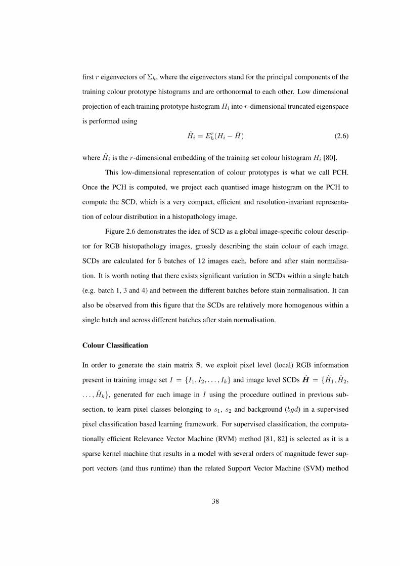
first r eigenvectors of Σh, where the eigenvectors stand for the principal components of the

training colour prototype histograms and are orthonormal to each other. Low dimensional

projection of each training prototype histogramHi into r-dimensional truncated eigenspace

is performed using

Hi = Erh(Hi − H) (2.6)

where Hi is the r-dimensional embedding of the training set colour histogram Hi [80].

This low-dimensional representation of colour prototypes is what we call PCH.

Once the PCH is computed, we project each quantised image histogram on the PCH to

compute the SCD, which is a very compact, efficient and resolution-invariant representa-

tion of colour distribution in a histopathology image.

Figure 2.6 demonstrates the idea of SCD as a global image-specific colour descrip-

tor for RGB histopathology images, grossly describing the stain colour of each image.

SCDs are calculated for 5 batches of 12 images each, before and after stain normalisa-

tion. It is worth noting that there exists significant variation in SCDs within a single batch

(e.g. batch 1, 3 and 4) and between the different batches before stain normalisation. It can

also be observed from this figure that the SCDs are relatively more homogenous within a

single batch and across different batches after stain normalisation.

Colour Classification

In order to generate the stain matrix S, we exploit pixel level (local) RGB information

present in training image set I = {I1, I2, . . . , Ik} and image level SCDs H = {H1, H2,

. . . , Hk}, generated for each image in I using the procedure outlined in previous sub-

section, to learn pixel classes belonging to s1, s2 and background (bgd) in a supervised

pixel classification based learning framework. For supervised classification, the computa-

tionally efficient Relevance Vector Machine (RVM) method [81, 82] is selected as it is a

sparse kernel machine that results in a model with several orders of magnitude fewer sup-

port vectors (and thus runtime) than the related Support Vector Machine (SVM) method

38

−0.2

−0.1

0

0.1

0.2

Batch−1

Batch−2

Batch−3

Batch−4

Batch−5

−0.2

−0.15

−0.1

−0.05

0

0.05

0.1

0.15

0.2

Batch−1

Batch−2

Batch−3

Batch−4

Batch−5

Figure 2.6: Boxplots represent the range of SCDs before (top) and after (bottom) stainnormalisation on 5 batches of training images (used in Section 2.4.2). Note that the SCDsare dispersed for batches of un-normalised images compared to the SCDs of normalisedimages.

[83]. Random Forests (RF) [84, 85] (of various sizes) were also evaluated, but their per-

formance was inferior as they tended to overfit the data. Additionally, the RVM provides

a probabilistic (rather than binary) output. As we have a 3-class problem, and RVM is a

2-class classifier, classification is implemented using the one-against-all approach [86, 87].

39

Given a feature vector F = [R, G, B, H] (generated by concatenating RGB

pixels values with corresponding image-specific SCD H) and pixel level class labels A,

we perform supervised machine learning to produce a probabilistic output that provides the

probability of association of each pixel to a particular class. Proportion of each stain at each

pixel location is computed by combining the probabilistic output obtained from the three

RVM classifiers, as follows:

P (sn|F ) =Psn(sn|F )

Ps1(s1|F ) + Ps2(s2|F ) + Pbgd(bgd|F )(2.7)

where sn ∈ {s1, s2, bgd}, Psn(sn|F ) is the probabilistic output of the RVM model.

P (sn|F ) is used to define the pixels of interest for each stain. Pixels assigned a

proportion greater than some threshold Tp are used to calculate the exemplar colour for

each stain. We use the mean colours (rn, gn, bn) of pixels classified as belonging to each

class to define stain colour, as shown in (2.8). If only 2 stains are used, the cross product of

[sr,1, sg,1, sb,1] and [sr,2, sg,2, sb,2] is used to complete the 3× 3 S matrix,

sr,n

sg,n

sb,n

=

− log(rn + 1)/256

− log(gn + 1)/256

− log(bn + 1)/256

/

∣∣∣∣∣∣∣∣∣∣

− log(rn + 1)/256

− log(gn + 1)/256

− log(bn + 1)/256

∣∣∣∣∣∣∣∣∣∣

(2.8)

Figure 2.7 shows examples of the probability maps produced by the stain matrix

estimation method (data taken from [76]). It can be seen that if no SCD [r = 0 in (2.6)]

is used (Figure 2.7 columns 2), significant probability is assigned to each class for weakly

stained pixels and background pixels with very minor staining. These are the pixels where

classification is context specific (i.e. it depends whether the overall staining is strong, or

weak). Magee et al.[76] showed that there was no statistically significant improvement (or

degradation) in classification accuracy when more than 1-dimensional (1D) SCD was used.

Therefore, in all our experiments, we employed 1D SCD for computation of stain matrix in

all our experiments.

40

H&E Sample

H&DAB Sample

Original Image No SCD 1-D SCD

Figure 2.7: Probability maps P(sn) for typical H&E (top) and H&DAB (bottom) stainedimages using classifiers with no SCD [r = 0 in (2.6)] (columns 2 ) and 1D SCD [r = 1in (2.6)] (columns 3). [White = high probability of belonging to the stain channel and viceversa] [76].

41

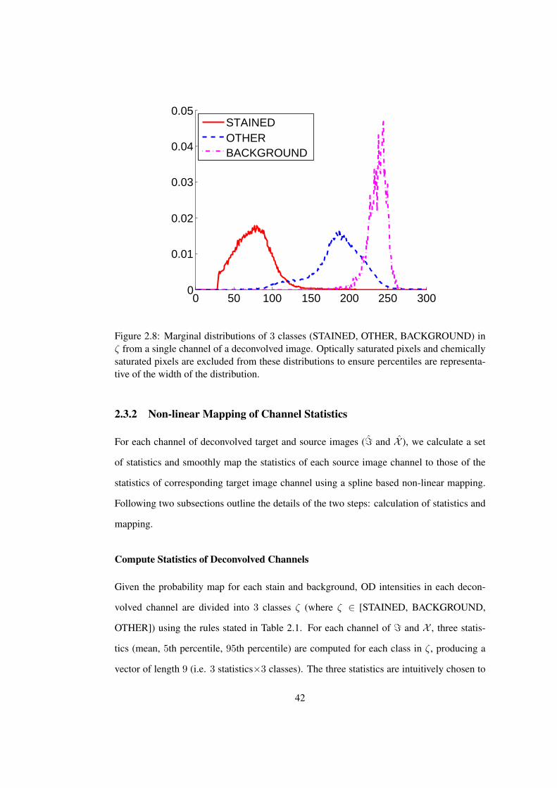
0 50 100 150 200 250 3000

0.01

0.02

0.03

0.04

0.05

STAINEDOTHERBACKGROUND

Figure 2.8: Marginal distributions of 3 classes (STAINED, OTHER, BACKGROUND) inζ from a single channel of a deconvolved image. Optically saturated pixels and chemicallysaturated pixels are excluded from these distributions to ensure percentiles are representa-tive of the width of the distribution.

2.3.2 Non-linear Mapping of Channel Statistics

For each channel of deconvolved target and source images (= and X ), we calculate a set

of statistics and smoothly map the statistics of each source image channel to those of the

statistics of corresponding target image channel using a spline based non-linear mapping.

Following two subsections outline the details of the two steps: calculation of statistics and

mapping.

Compute Statistics of Deconvolved Channels

Given the probability map for each stain and background, OD intensities in each decon-

volved channel are divided into 3 classes ζ (where ζ ∈ [STAINED, BACKGROUND,

OTHER]) using the rules stated in Table 2.1. For each channel of = and X , three statis-

tics (mean, 5th percentile, 95th percentile) are computed for each class in ζ, producing a

vector of length 9 (i.e. 3 statistics×3 classes). The three statistics are intuitively chosen to

42

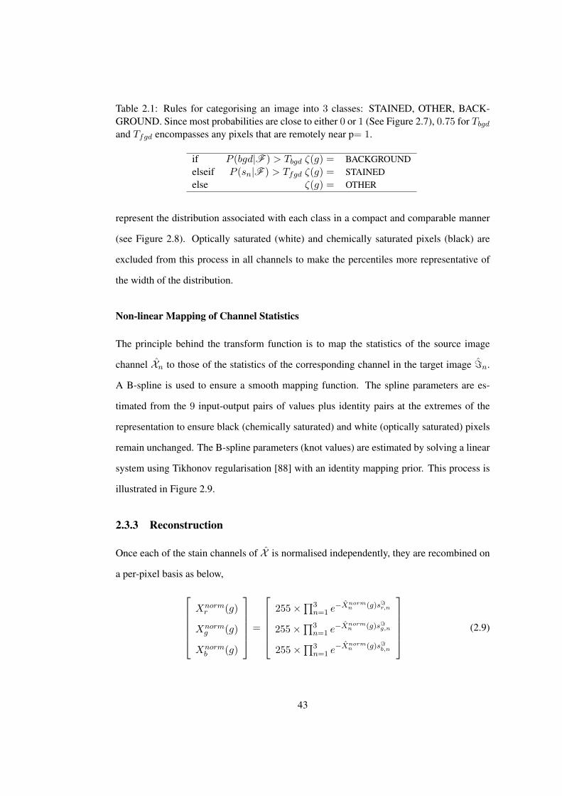
Table 2.1: Rules for categorising an image into 3 classes: STAINED, OTHER, BACK-GROUND. Since most probabilities are close to either 0 or 1 (See Figure 2.7), 0.75 for Tbgdand Tfgd encompasses any pixels that are remotely near p= 1.

if P (bgd|F ) > Tbgd ζ(g) = BACKGROUNDelseif P (sn|F ) > Tfgd ζ(g) = STAINEDelse ζ(g) = OTHER

represent the distribution associated with each class in a compact and comparable manner

(see Figure 2.8). Optically saturated (white) and chemically saturated pixels (black) are

excluded from this process in all channels to make the percentiles more representative of

the width of the distribution.

Non-linear Mapping of Channel Statistics

The principle behind the transform function is to map the statistics of the source image

channel Xn to those of the statistics of the corresponding channel in the target image =n.

A B-spline is used to ensure a smooth mapping function. The spline parameters are es-

timated from the 9 input-output pairs of values plus identity pairs at the extremes of the

representation to ensure black (chemically saturated) and white (optically saturated) pixels

remain unchanged. The B-spline parameters (knot values) are estimated by solving a linear

system using Tikhonov regularisation [88] with an identity mapping prior. This process is

illustrated in Figure 2.9.

2.3.3 Reconstruction

Once each of the stain channels of X is normalised independently, they are recombined on

a per-pixel basis as below,

Xnormr (g)

Xnormg (g)

Xnormb (g)

=

255×∏3n=1 e

−Xnormn (g)s=r,n

255×∏3n=1 e

−Xnormn (g)s=g,n

255×∏3n=1 e

−Xnormn (g)s=b,n

(2.9)

43

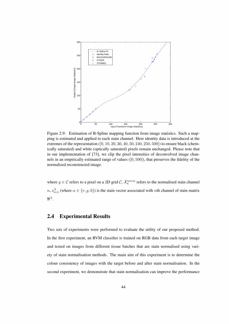
0 50 100 150 200 250 3000

50

100

150

200

250

300

Input [Transform Image Statistics]

Out

put [

Tar

get I

mag

e S

tatis

tics]

B−Spline FitIdentity DataBACKGROUNDOTHERSTAINED

Figure 2.9: Estimation of B-Spline mapping function from image statistics. Such a map-ping is estimated and applied to each stain channel. Here identity data is introduced at theextremes of the representation ([0, 10, 20, 30, 40, 50, 240, 250, 500]) to ensure black (chem-ically saturated) and white (optically saturated) pixels remain unchanged. Please note thatin our implementation of [73], we clip the pixel intensities of deconvolved image chan-nels in an empirically estimated range of values ([0, 500]), that preserves the fidelity of thenormalised reconstructed image.

where g ∈ C refers to a pixel on a 2D grid C, X normn refers to the normalised stain channel

n, s=α,n (where α ∈ {r, g, b}) is the stain vector associated with nth channel of stain matrix

S=.

2.4 Experimental Results

Two sets of experiments were performed to evaluate the utility of our proposed method.

In the first experiment, an RVM classifier is trained on RGB data from each target image

and tested on images from different tissue batches that are stain normalised using vari-

ety of stain normalisation methods. The main aim of this experiment is to determine the

colour consistency of images with the target before and after stain normalisation. In the

second experiment, we demonstrate that stain normalisation can improve the performance

44

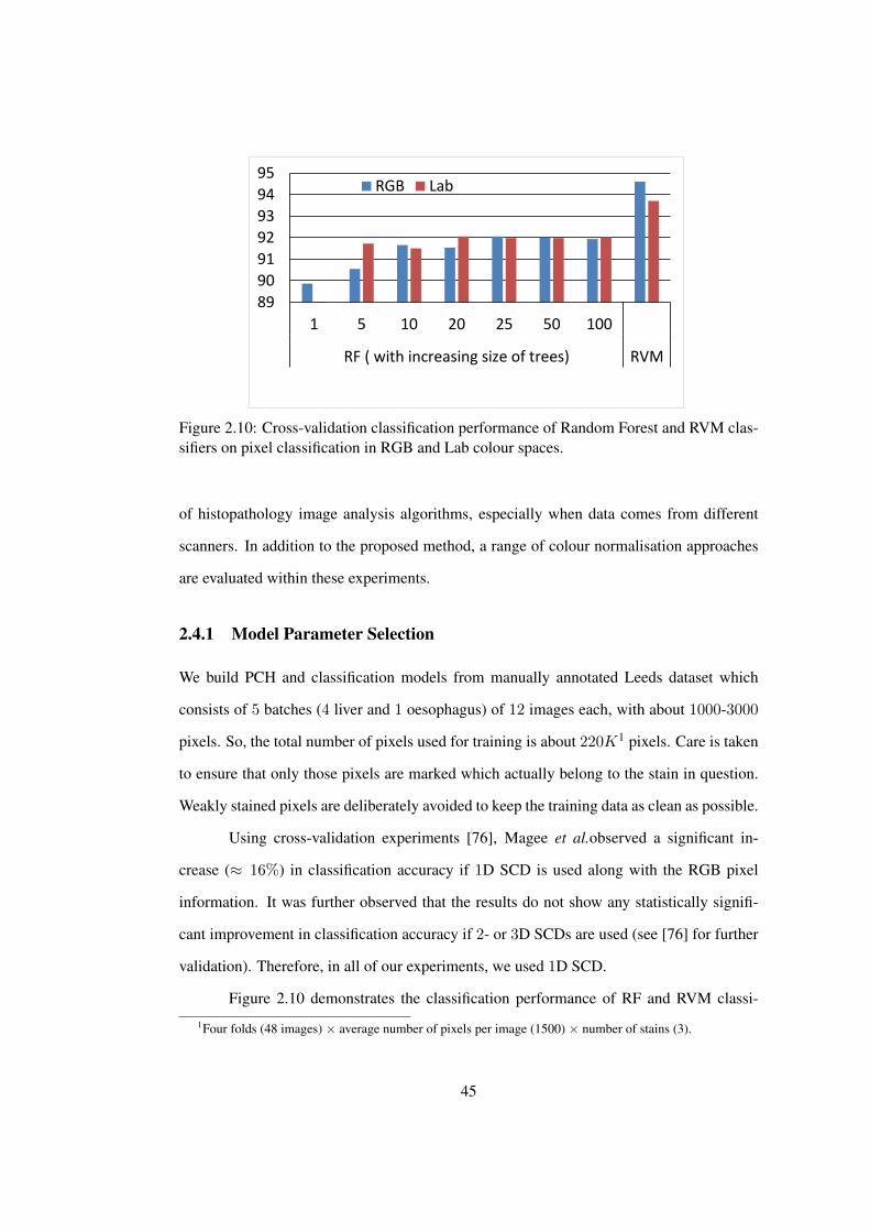
89

90

91

92

93

94

95

1 5 10 20 25 50 100

RF ( with increasing size of trees) RVM

RGB Lab

Figure 2.10: Cross-validation classification performance of Random Forest and RVM clas-sifiers on pixel classification in RGB and Lab colour spaces.

of histopathology image analysis algorithms, especially when data comes from different

scanners. In addition to the proposed method, a range of colour normalisation approaches

are evaluated within these experiments.

2.4.1 Model Parameter Selection

We build PCH and classification models from manually annotated Leeds dataset which

consists of 5 batches (4 liver and 1 oesophagus) of 12 images each, with about 1000-3000

pixels. So, the total number of pixels used for training is about 220K1 pixels. Care is taken

to ensure that only those pixels are marked which actually belong to the stain in question.

Weakly stained pixels are deliberately avoided to keep the training data as clean as possible.

Using cross-validation experiments [76], Magee et al.observed a significant in-

crease (≈ 16%) in classification accuracy if 1D SCD is used along with the RGB pixel

information. It was further observed that the results do not show any statistically signifi-

cant improvement in classification accuracy if 2- or 3D SCDs are used (see [76] for further

validation). Therefore, in all of our experiments, we used 1D SCD.

Figure 2.10 demonstrates the classification performance of RF and RVM classi-1Four folds (48 images) × average number of pixels per image (1500) × number of stains (3).

45

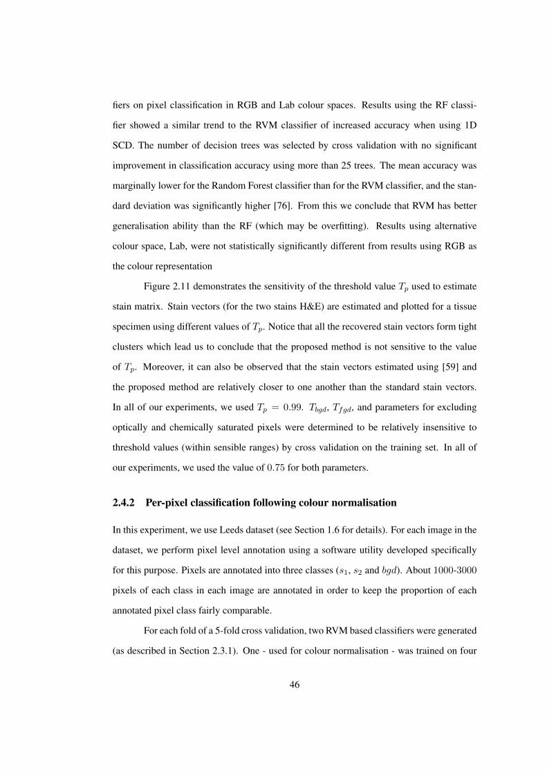
fiers on pixel classification in RGB and Lab colour spaces. Results using the RF classi-

fier showed a similar trend to the RVM classifier of increased accuracy when using 1D

SCD. The number of decision trees was selected by cross validation with no significant

improvement in classification accuracy using more than 25 trees. The mean accuracy was

marginally lower for the Random Forest classifier than for the RVM classifier, and the stan-

dard deviation was significantly higher [76]. From this we conclude that RVM has better

generalisation ability than the RF (which may be overfitting). Results using alternative

colour space, Lab, were not statistically significantly different from results using RGB as

the colour representation

Figure 2.11 demonstrates the sensitivity of the threshold value Tp used to estimate

stain matrix. Stain vectors (for the two stains H&E) are estimated and plotted for a tissue

specimen using different values of Tp. Notice that all the recovered stain vectors form tight

clusters which lead us to conclude that the proposed method is not sensitive to the value

of Tp. Moreover, it can also be observed that the stain vectors estimated using [59] and

the proposed method are relatively closer to one another than the standard stain vectors.

In all of our experiments, we used Tp = 0.99. Tbgd, Tfgd, and parameters for excluding

optically and chemically saturated pixels were determined to be relatively insensitive to

threshold values (within sensible ranges) by cross validation on the training set. In all of

our experiments, we used the value of 0.75 for both parameters.

2.4.2 Per-pixel classification following colour normalisation

In this experiment, we use Leeds dataset (see Section 1.6 for details). For each image in the

dataset, we perform pixel level annotation using a software utility developed specifically

for this purpose. Pixels are annotated into three classes (s1, s2 and bgd). About 1000-3000

pixels of each class in each image are annotated in order to keep the proportion of each

annotated pixel class fairly comparable.

For each fold of a 5-fold cross validation, two RVM based classifiers were generated

(as described in Section 2.3.1). One - used for colour normalisation - was trained on four

46

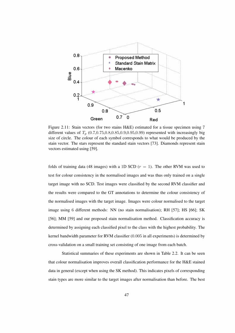
Figure 2.11: Stain vectors (for two stains H&E) estimated for a tissue specimen using 7different values of Tp (0.7,0.75,0.8,0.85,0.9,0.95,0.99) represented with increasingly bigsize of circle. The colour of each symbol corresponds to what would be produced by thestain vector. The stars represent the standard stain vectors [73]. Diamonds represent stainvectors estimated using [59].

folds of training data (48 images) with a 1D SCD (r = 1). The other RVM was used to

test for colour consistency in the normalised images and was thus only trained on a single

target image with no SCD. Test images were classified by the second RVM classifier and

the results were compared to the GT annotations to determine the colour consistency of

the normalised images with the target image. Images were colour normalised to the target

image using 6 different methods: NN (no stain normalisation); RH [57]; HS [66]; SK

[56]; MM [59] and our proposed stain normalisation method. Classification accuracy is

determined by assigning each classified pixel to the class with the highest probability. The

kernel bandwidth parameter for RVM classifier (0.005 in all experiments) is determined by

cross-validation on a small training set consisting of one image from each batch.

Statistical summaries of these experiments are shown in Table 2.2. It can be seen

that colour normalisation improves overall classification performance for the H&E stained

data in general (except when using the SK method). This indicates pixels of corresponding

stain types are more similar to the target images after normalisation than before. The best

47

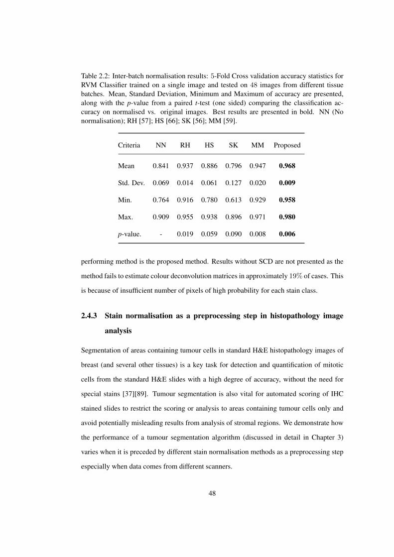
Table 2.2: Inter-batch normalisation results: 5-Fold Cross validation accuracy statistics forRVM Classifier trained on a single image and tested on 48 images from different tissuebatches. Mean, Standard Deviation, Minimum and Maximum of accuracy are presented,along with the p-value from a paired t-test (one sided) comparing the classification ac-curacy on normalised vs. original images. Best results are presented in bold. NN (Nonormalisation); RH [57]; HS [66]; SK [56]; MM [59].

Criteria NN RH HS SK MM Proposed

Mean 0.841 0.937 0.886 0.796 0.947 0.968

Std. Dev. 0.069 0.014 0.061 0.127 0.020 0.009

Min. 0.764 0.916 0.780 0.613 0.929 0.958

Max. 0.909 0.955 0.938 0.896 0.971 0.980

p-value. - 0.019 0.059 0.090 0.008 0.006

performing method is the proposed method. Results without SCD are not presented as the

method fails to estimate colour deconvolution matrices in approximately 19% of cases. This

is because of insufficient number of pixels of high probability for each stain class.

2.4.3 Stain normalisation as a preprocessing step in histopathology image

analysis

Segmentation of areas containing tumour cells in standard H&E histopathology images of

breast (and several other tissues) is a key task for detection and quantification of mitotic

cells from the standard H&E slides with a high degree of accuracy, without the need for

special stains [37][89]. Tumour segmentation is also vital for automated scoring of IHC

stained slides to restrict the scoring or analysis to areas containing tumour cells only and

avoid potentially misleading results from analysis of stromal regions. We demonstrate how

the performance of a tumour segmentation algorithm (discussed in detail in Chapter 3)

varies when it is preceded by different stain normalisation methods as a preprocessing step

especially when data comes from different scanners.

48

We use the public MITOS dataset (see Section 1.6 for details) of BC histopathology

images [41]. In order to account for inter-observer variability, all images are hand seg-

mented by two expert pathologists to mark the boundary of tumor areas in each HPF. The

average degree of disagreement (inter-observer variability) between the two pathologists on

GT images is 11.55% ± 0.05. We generate all experimental results on 2 criteria: (1) con-

sidering pathologist-1’s markings (Path-1) as GT; (2) considering pathologist-2’s markings

(Path-2) as GT.

All images in the dataset were colour normalised by a range of methods in the same

way as Section 2.4.2 using a target image scanned using an Aperio scanner. The segmen-

tation was performed using [89] trained on data from the Aperio scanner and evaluated

by cross validation against the manual annotations. The classifier for colour normalisation

using the presented method was trained on the data from Section 2.4.2.

Segmentation performance was evaluated using the Dice coefficient; a widely used

pixel-wise accuracy measure. Given a segmented image (X) and pathologist’s marked GT

image (Y ), Dice coefficient is defined by 2|X∩Y ||X|+|Y | . The measure provides values between

0.0 to 1.0 (1.0 indicates identical segmentations).

Figure 2.12 provides illustration of different stain normalisation methods consid-

ered in this study. It can be seen that when RH stain normalisation is applied (on both

Aperio and Hamamatsu HPF images), output image quality degrades significantly partic-

ularly in areas where we have fat tissue (white regions) and flat stromal structures of the

tissue. For Hamamatsu HPF images, the effect of stain normalisation is almost invisible

in the case of RH and SK. With MM, the effect of image normalisation is relatively dis-

cernible, however there are two problems: (1) the colour distribution of normalised image

is different from the target image as the method normalised both source and target image;

(2) for Hamamatsu HPF image, it introduces significant visual artifacts in white regions (see

electronic version for better visibility). The reason being the linear transformation function

which do not faithfully normalise extremely white and extremely dark pixels. With the

proposed method, we obtain visually superior colour normalisation: staining of both Eosin

49

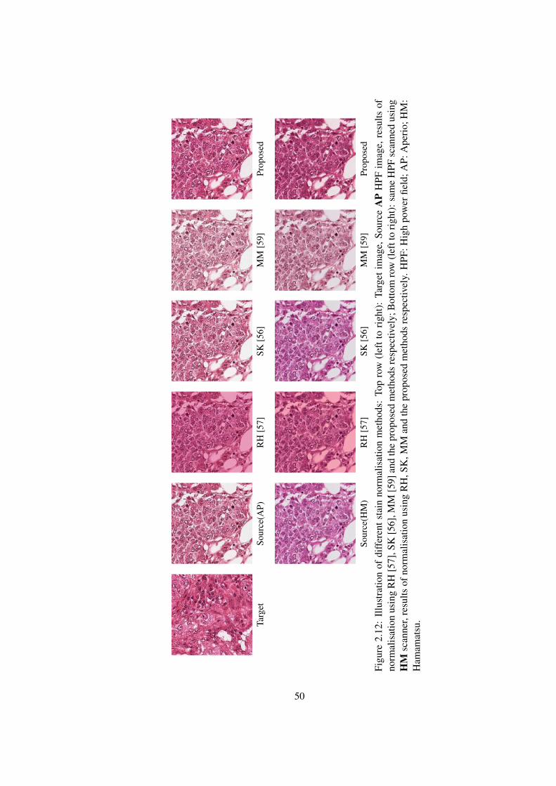
Targ

etSo

urce

(AP)

RH

[57]

SK[5

6]M

M[5

9]Pr

opos

ed

Sour

ce(H

M)

RH

[57]

SK[5

6]M

M[5

9]Pr

opos

ed

Figu

re2.

12:

Illu

stra

tion

ofdi

ffer

ents

tain

norm

alis

atio

nm

etho

ds:

Top

row

(lef

tto

righ

t):

Targ

etim

age,

Sour

ceA

PH

PFim

age,

resu

ltsof

norm

alis

atio

nus

ing

RH

[57]

,SK

[56]

,MM

[59]

and

the

prop

osed

met

hods

resp

ectiv

ely;

Bot

tom

row

(lef

tto

righ

t):s

ame

HPF

scan

ned

usin

gH

Msc

anne

r,re

sults

ofno

rmal

isat

ion

usin

gR

H,S

K,M

Man

dth

epr

opos

edm

etho

dsre

spec

tivel

y.H

PF:H

igh

pow

erfie

ld;A

P:A

peri

o;H

M:

Ham

amat

su.

50

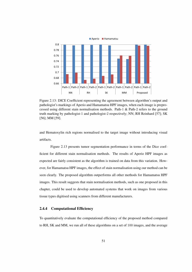
0.66

0.68

0.7

0.72

0.74

0.76

0.78

0.8

Path-1 Path-2 Path-1 Path-2 Path-1 Path-2 Path-1 Path-2 Path-1 Path-2

NN RH SK MM Proposed

Aperio Hamamatsu

Figure 2.13: DICE Coefficient representing the agreement between algorithm’s output andpathologist’s markings of Aperio and Hamamatsu HPF images, when each image is prepro-cessed using different stain normalisation methods. Path-1 & Path-2 refers to the groundtruth marking by pathologist-1 and pathologist-2 respectively; NN; RH Reinhard [57]; SK[56]; MM [59].

and Hematoxylin rich regions normalised to the target image without introducing visual

artifacts.

Figure 2.13 presents tumor segmentation performance in terms of the Dice coef-

ficient for different stain normalisation methods. The results of Aperio HPF images as

expected are fairly consistent as the algorithm is trained on data from this variation. How-

ever, for Hamamatsu HPF images, the effect of stain normalisation using our method can be

seen clearly. The proposed algorithm outperforms all other methods for Hamamatsu HPF

images. This result suggests that stain normalisation methods, such as one proposed in this

chapter, could be used to develop automated systems that work on images from various

tissue types digitised using scanners from different manufacturers.

2.4.4 Computational Efficiency

To quantitatively evaluate the computational efficiency of the proposed method compared

to RH, SK and MM, we run all of these algorithms on a set of 100 images, and the average

51

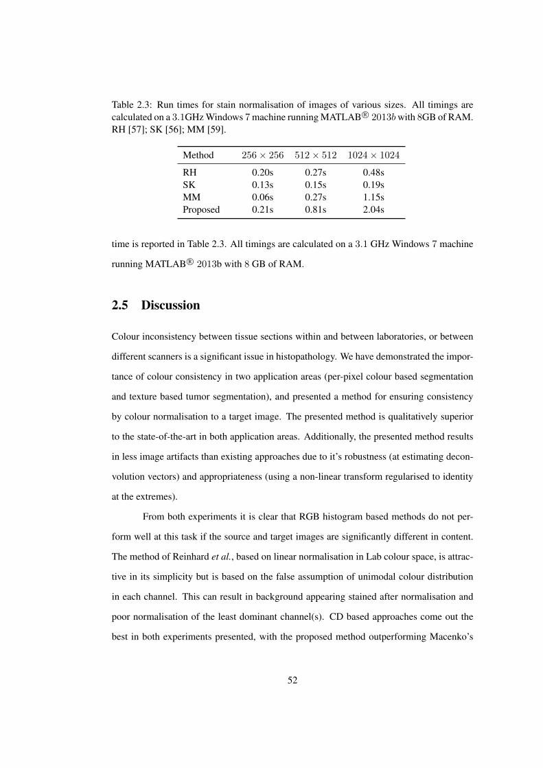
Table 2.3: Run times for stain normalisation of images of various sizes. All timings arecalculated on a 3.1GHz Windows 7 machine running MATLAB R© 2013bwith 8GB of RAM.RH [57]; SK [56]; MM [59].

Method 256× 256 512× 512 1024× 1024

RH 0.20s 0.27s 0.48sSK 0.13s 0.15s 0.19sMM 0.06s 0.27s 1.15sProposed 0.21s 0.81s 2.04s

time is reported in Table 2.3. All timings are calculated on a 3.1 GHz Windows 7 machine

running MATLAB R© 2013b with 8 GB of RAM.

2.5 Discussion

Colour inconsistency between tissue sections within and between laboratories, or between

different scanners is a significant issue in histopathology. We have demonstrated the impor-

tance of colour consistency in two application areas (per-pixel colour based segmentation

and texture based tumor segmentation), and presented a method for ensuring consistency

by colour normalisation to a target image. The presented method is qualitatively superior

to the state-of-the-art in both application areas. Additionally, the presented method results

in less image artifacts than existing approaches due to it’s robustness (at estimating decon-

volution vectors) and appropriateness (using a non-linear transform regularised to identity

at the extremes).

From both experiments it is clear that RGB histogram based methods do not per-

form well at this task if the source and target images are significantly different in content.

The method of Reinhard et al., based on linear normalisation in Lab colour space, is attrac-

tive in its simplicity but is based on the false assumption of unimodal colour distribution

in each channel. This can result in background appearing stained after normalisation and

poor normalisation of the least dominant channel(s). CD based approaches come out the

best in both experiments presented, with the proposed method outperforming Macenko’s

52

method in both cases. The appropriateness of CD based approaches should be obvious,

as chemical processes are largely independent for each stain, and CD separates out the ef-

fect of variation of each stain so it can be corrected independently. Of the two CD based

approaches evaluated, the method presented herein is superior (Figure 2.3). This could

be for two reasons; (i) Better, or more robust deconvolution matrix estimation, and/or (ii)

a more appropriate mapping function. An investigation on a small number of images re-

vealed that both the proposed (supervised classification based) method and Macenko et al.’s

(unsupervised) method generally produced more appropriate deconvolution matrices than

simply using standard matrices, with little data leaking into the 3rd channel (Figure 2.14).

The proposed method performed marginally better under this criterion than the approach

of Macenko et al., with consistent performance over all images. However, we speculate

that the inappropriateness of the simple linear mapping function used in the work (espe-

cially at the extremes of distributions) is the main reason for the superior performance of

our approach, as our method seems reasonably invariant to the choice of thresholds (and

thus slight variation in deconvolution matrices), and the matrices produced by Macenko et

al. are not radically different in most cases.

It is worth pointing out that in Section 2.4.3 the tissue type (breast tissue) was

significantly different to the tissue used for training the classifier for our method (liver

and oesophagus). However, the performance on this new set was nonetheless accurate and

robust. This suggests that the proposed method is potentially appropriate for a wide variety

of applications without re-training.

One important point to raise about the use of any colour normalisation method

which is based on a target image is the choice of an appropriate target image. The choice

of target image in our experiments was either random (Section 2.4.2), or based on manual

selection (Section 2.4.3). In practice however, careful choice of the target image based on

quantitative measures (e.g. cross validation accuracy of some method) applied to a set of

normalised images may be required, as performance of a method on a single target image

is not necessarily indicative of performance on a normalised image set.

53

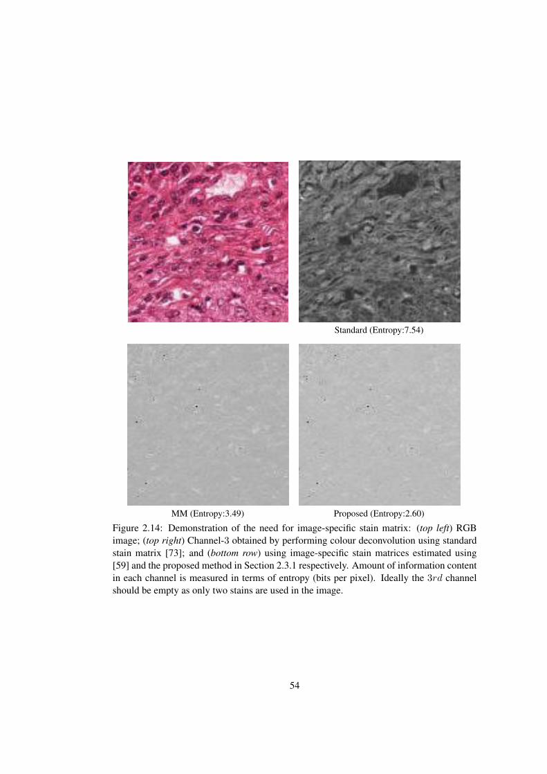
Standard (Entropy:7.54)

MM (Entropy:3.49) Proposed (Entropy:2.60)

Figure 2.14: Demonstration of the need for image-specific stain matrix: (top left) RGBimage; (top right) Channel-3 obtained by performing colour deconvolution using standardstain matrix [73]; and (bottom row) using image-specific stain matrices estimated using[59] and the proposed method in Section 2.3.1 respectively. Amount of information contentin each channel is measured in terms of entropy (bits per pixel). Ideally the 3rd channelshould be empty as only two stains are used in the image.

54

It remains true that often the best way of estimating stain vectors is to apply a

single stain to control tissue [73]. This is the method used to estimate the standard matrices

supplied with the publicly available implementations2 of [73]. However, it is often hard

to ensure that this control tissue is representative of tissue being analysed (especially over

time, or if analysis involves tissue from multiple labs/technicians). Colour normalisation

methods, such as those presented in this paper, offer an opportunity to utilise such carefully

estimated stain matrices over a wider range of tissues.

2.6 Summary

Histopathology diagnosis is based on visual examination of the morphology of histological

sections under a microscope. With the increasing popularity of digital slide scanners, deci-

sion support systems based on the analysis of digital pathology images are in high demand.

However, computerised decision support systems are fraught with problems that stem from

colour variations in tissue appearance mainly due to variation in tissue preparation, stain

reactivity from different manufacturers or different batches from the same manufacturer,

user or protocol variation and image acquisition with scanners from different manufactur-

ers. In this chapter, we presented a novel approach to stain normalisation in histopathology

images. The method is based on non-linear mapping of a source image to a target image

using a representation derived from CD. The method has been evaluated on two datasets:

one captures within-scanner variation between slides prepared at different times by differ-

ent technicians using stains (chemicals) from different batches, while another captures the

inter-scanner variation by scanning the same slide using two different scanners. The ex-

perimental results suggest that the paradigm of colour normalisation, as a preprocessing

step, can significantly help histological image analysis algorithms to demonstrate stable

performance which is insensitive to imaging conditions in general and scanner variations in

particular.

2http://www.math-info.univ-paris5.fr/˜lomn/Cours/TI/Material/Data/plugins/G_%20Landini’s%20Software.htm

55

Chapter 3

Tumour Segmentation

Segmentation of areas containing tumour cells in standard H&E histopathology images of

breast (and several other tissues) is a key task for computer-assisted assessment and grading

of histopathology slides. Good segmentation of tumour regions can not only highlight

slide-areas consisting of tumour cells, it is also vital for automated scoring of IHC stained

slides to restrict the scoring or analysis to areas containing tumour cells only and avoid

potentially misleading results from analysis of stromal regions. Furthermore, detection of

mitotic cells is critical for calculating key measures such as mitotic index, a key criterion

for grading several types of cancers including BC. We show in the next chapter that tumour

segmentation can allow detection and quantification of mitotic cells from the standard H&E

slides with a high degree of accuracy, without need for special stains, in turn making the

whole process more cost-effective.

3.1 Related Work

While some algorithms for segmentation of tumour nuclei [90], quantitative evaluation of

nuclear pleomorphism [91], detection and grading of lymphocytic infiltration in histopathol-

ogy images [49], and automated malignancy detection [92] have been reported in the liter-

ature, tumour segmentation in BC histopathology images has not received much attention.

57

There is a small body of literature available on tumour segmentation in tissue microarray

(TMA1) spots [93, 94, 95, 96, 97, 98, 99, 100]. These approaches can be broadly divided

into two classes: supervised approaches [93, 94, 95, 96, 97], and weakly supervised ap-

proaches [99, 100].

In [93], Wang et al. proposed a supervised tumour segmentation approach, that

exploits architectural and textural features of histological tissues in a Markov random field

based Bayesian estimation framework. Nuclei architecture features are extracted by seg-

menting a hematoxylin content image, obtained using CD framework [73]. Texture features

are extracted from the blue channel of the RGB image. Segmentation of tumour regions is

performed by energy minimisation using Metropolis algorithm [101].

Akbar et al. [94, 95] use rotation invariant context features, which they call spin-

context, to perform tumour segmentation in TMA spots. Spin-context combines affine-

invariant texture features, proposed in [102], and auto-context features, proposed in [103,

104], to obtain rotation invariant texture segmentation. A spin feature [102] encodes the

distribution of intensities within a circular support, while an auto-context learns contextual

probability/confidence map in an iterative manner, where the term ‘auto’ refers to the fact

that probability map learned at current iteration is used as input in the subsequent iteration.

A major drawback of supervised tumour segmentation approaches is the requirement of

large amount of high quality manually delineated pixel level annotation, which is generally

very difficult to obtain.

Xu et al. [99, 100] propose a weakly supervised machine learning approach in line

with multiple instance learning [105], an active area of research in machine learning com-

munity [106, 107], with strong applications in medical domain as well [108, 109, 110].

From a given set of densely sampled image patches, the framework generates bags of in-

stances where each instance is an image patch. Using multiple instance learning framework,

classification models are learned, which in turn, generate several classifiers for patch level1TMA is an array of tissue cores assembled on a single glass slide to allow simultaneous histological analy-

sis. As tissue microarray spots are prepared and stained simultaneously, they are generally less prone to stainingvariation as compared to standard histological slides.

58

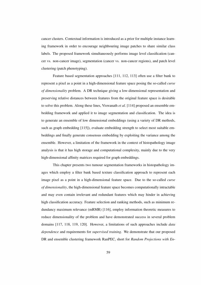
cancer clusters. Contextual information is introduced as a prior for multiple instance learn-

ing framework in order to encourage neighbouring image patches to share similar class

labels. The proposed framework simultaneously performs image level classification (can-

cer vs. non-cancer image), segmentation (cancer vs. non-cancer regions), and patch level

clustering (patch phenotyping).

Feature based segmentation approaches [111, 112, 113] often use a filter bank to

represent a pixel as a point in a high-dimensional feature space posing the so-called curse

of dimensionality problem. A DR technique giving a low-dimensional representation and

preserving relative distances between features from the original feature space is desirable

to solve this problem. Along these lines, Viswanath et al. [114] proposed an ensemble em-

bedding framework and applied it to image segmentation and classification. The idea is

to generate an ensemble of low dimensional embeddings (using a variety of DR methods,

such as graph embedding [115]), evaluate embedding strength to select most suitable em-

beddings and finally generate consensus embedding by exploiting the variance among the

ensemble. However, a limitation of the framework in the context of histopathology image

analysis is that it has high storage and computational complexity, mainly due to the very

high-dimensional affinity matrices required for graph embeddings.

This chapter presents two tumour segmentation frameworks in histopathology im-

ages which employ a filter bank based texture classification approach to represent each

image pixel as a point in a high-dimensional feature space. Due to the so-called curse

of dimensionality, the high-dimensional feature space becomes computationally intractable

and may even contain irrelevant and redundant features which may hinder in achieving

high classification accuracy. Feature selection and ranking methods, such as minimum re-

dundancy maximum relevance (mRMR) [116], employ information theoretic measures to

reduce dimensionality of the problem and have demonstrated success in several problem

domains [117, 118, 119, 120]. However, a limitations of such approaches include data

dependence and requirements for supervised training. We demonstrate that our proposed

DR and ensemble clustering framework RanPEC, short for Random Projections with En-

59

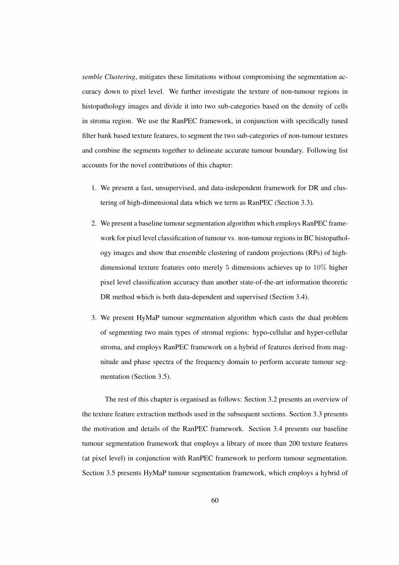
semble Clustering, mitigates these limitations without compromising the segmentation ac-

curacy down to pixel level. We further investigate the texture of non-tumour regions in

histopathology images and divide it into two sub-categories based on the density of cells

in stroma region. We use the RanPEC framework, in conjunction with specifically tuned

filter bank based texture features, to segment the two sub-categories of non-tumour textures

and combine the segments together to delineate accurate tumour boundary. Following list

accounts for the novel contributions of this chapter:

1. We present a fast, unsupervised, and data-independent framework for DR and clus-

tering of high-dimensional data which we term as RanPEC (Section 3.3).

2. We present a baseline tumour segmentation algorithm which employs RanPEC frame-

work for pixel level classification of tumour vs. non-tumour regions in BC histopathol-

ogy images and show that ensemble clustering of random projections (RPs) of high-

dimensional texture features onto merely 5 dimensions achieves up to 10% higher

pixel level classification accuracy than another state-of-the-art information theoretic

DR method which is both data-dependent and supervised (Section 3.4).

3. We present HyMaP tumour segmentation algorithm which casts the dual problem

of segmenting two main types of stromal regions: hypo-cellular and hyper-cellular

stroma, and employs RanPEC framework on a hybrid of features derived from mag-

nitude and phase spectra of the frequency domain to perform accurate tumour seg-

mentation (Section 3.5).

The rest of this chapter is organised as follows: Section 3.2 presents an overview of

the texture feature extraction methods used in the subsequent sections. Section 3.3 presents

the motivation and details of the RanPEC framework. Section 3.4 presents our baseline

tumour segmentation framework that employs a library of more than 200 texture features

(at pixel level) in conjunction with RanPEC framework to perform tumour segmentation.

Section 3.5 presents HyMaP tumour segmentation framework, which employs a hybrid of

60

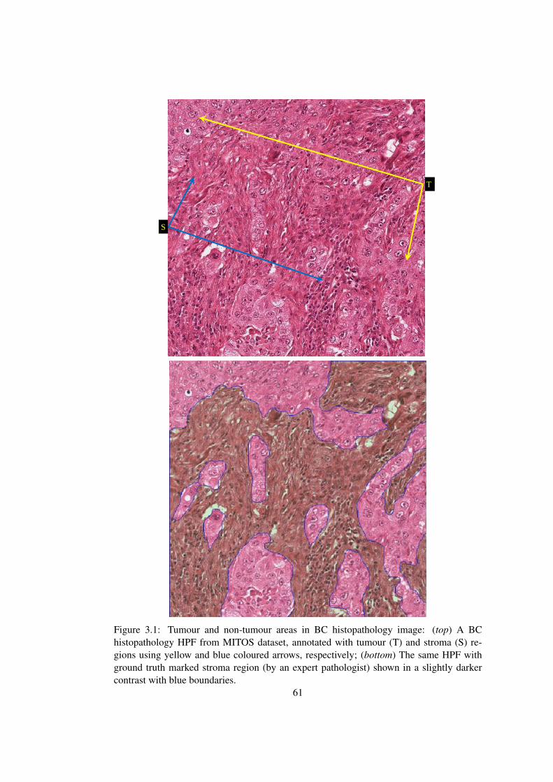
T

S

Figure 3.1: Tumour and non-tumour areas in BC histopathology image: (top) A BChistopathology HPF from MITOS dataset, annotated with tumour (T) and stroma (S) re-gions using yellow and blue coloured arrows, respectively; (bottom) The same HPF withground truth marked stroma region (by an expert pathologist) shown in a slightly darkercontrast with blue boundaries.

61

magnitude and phase spectra of Gabor filter bank to perform tumour segmentation. Section

3.6 summarises the chapter with a brief overview of the methods and results presented in

this chapter.

3.2 Texture Features for Tumour Segmentation

Frequency domain representation of an image, generally obtained using Fourier transform

[121], provides a wealth of information related to the presence or absence of particular

frequencies in the image. Frequency domain features are of particular interest in texture

analysis, as textures are generally constituted of a significant number of similar looking

regularly arranged primitives which give rise to the perception of homogeneity. This is

the reason, why frequency domain analysis of textures is the most common approach to

perform texture segmentation and classification [122, 123, 124].

A traditional approach to texture segmentation is to characterise an image with a

bank of texture filters [111, 112, 113] to generate a set of features that are capable of dis-

criminating texture patterns belonging to different texture classes. Thus, patterns belonging

to each class will form a cluster in the feature space which is compact and isolated from

clusters corresponding to all the other texture classes. Tumour segmentation algorithms,

presented in Section 3.4 and 3.5, utilise frequency domain texture features that are derived

from Gabor [125], phase gradients [126], orientation pyramid [127], and full wavelet packet

[128] texture analysis frameworks. Therefore, in this section we briefly describe these tex-

ture feature extraction frameworks.

3.2.1 Gabor Texture Features

A Gabor filter bank [125], named after Dennis Gabor, is a set of linear filters that are

widely used in image processing literature for performing variety of tasks including texture

segmentation [129, 130], face recognition [131, 132] and edge detection [113, 133, 134,

135]. Gabor filter bank is related to the Fourier transform in the sense that Gabor transform

62

coefficients correspond to particular band of frequencies in particular range of directions

only. Frequency and orientation representations of Gabor filters are similar to those of the

human visual system as well, and they have been found to be particularly appropriate for

texture representation and discrimination [125].

The log-Gabor function proposed by [136] is generally used as an improved form

of the standard Gabor function mainly because of two important characteristics: (1) they

do not contain any DC component; and (2) the transfer function is extendable in frequency

range, thus providing broad spectral information with maximal spatial localisation. Due to

the limitation of log function at origin, log-Gabor filters are formulated in the frequency

domain. In a polar coordinate system, 2D log-Gabor filters can be split into the radial and

angular components, defined by the following equation,

G (θ, ω) = exp

{− [log(ω/ω0)]2

2 · [log(σω)]2

}· exp

{−(θ − θ0)2

2 · σ2θ

}, (3.1)

where ω0 is centre frequency, θ0 is the orientation angle, σω and σθ are radial and angular

bandwidth parameters.

In general, the parameters ω and θ constitute the parameter space of Gabor filter

bank. The parameters ω and θ represent frequency and orientation of the 2D Gabor filter

respectively, where θ ∈ Θ, a set of possible orientations, and ω ∈ F , a set of possible

frequencies. We investigated the low, intermediate and high frequency bands of the Gabor

spectrum and found that the features in the intermediate frequency bands are most discrim-

inative for texture segmentation in BC histopathology images. The set of orientations Θ,

generally varies between 0 and π in regular intervals. In our experiments, we observed im-

proved performance by using orientation separation of 30 ◦, which generates a filter bank at

following orientations: Θ = {0 ◦, 30 ◦, 60 ◦, 90 ◦, 120 ◦, and 150 ◦}.

Given an image I = (C, Ψ) with centred Fourier transform Iω = F(I), response

V i of the i-th Gabor filter G i to the image I is calculated in frequency and spatial domains

63

as follows,

V iω = IωG i (3.2)

V i = F−1[V iω

](3.3)

where F−1 denotes inverse Fourier transform operation, i = 1, 2, · · · , |Θ| × |F | and |.|

denotes the cardinality of the set. The filter responses are passed through a sigmoidal func-

tion followed by a smoothing function to introduce non-linearity in the computed features

[112, 129].

3.2.2 Phase Gradient Texture Features

Gabor texture features are motivated by the fact that the image coding in the mammalian

visual system is also performed in a very similar manner, that is, by means of cells that are

tuned to specific frequencies and orientations [125]. This information embedded in Gabor

spectrum is extensively exploited and found to be very useful in various studies mainly

focusing on texture discrimination. In addition to these cells, primary visual cortex is com-

posed of antagonistic cells, which have a phase shift of 90 ◦ and have spatial profiles of

receptive fields which can be described by the real and imaginary parts of a Gabor impulse

response [137]. This gives rise to the intuition that local phase information is encoded, and

thus implicitly utilised, in visual system as well.

Unfortunately, calculating phase information is not straight forward. A classical

approach to computing phase is to apply the inverse tangent operation to the real and com-

plex parts of the Gabor spectrum. However, if a filtered image contains isolated zero

points in both real and imaginary parts, phase is not defined on such points. This gives

rise to a very well known mathematical problem commonly referred to as phase wrapping

[126, 138]. Kovesi et al.proposed to use edge based characterisation of image to calculate

local phase [139]. However, we use the approach proposed in [140] that employs texture

based characterisation of image and exploit indirect phase gradients which provide efficient

64

way of estimating instantaneous frequency in 2D.

Concretely, log-Gabor filters are used to decompose a given image into scale and

orientation components [136, 141]. If V i(x, y) denotes the convolution response of a 2D

image I(x, y) to the i-th log-Gabor filter G i (3.3).The same relationship can be indirectly

represented as,

V i(x, y) =∣∣V i(x, y)

∣∣ exp(jφi(x, y)) (3.4)

where |·| denotes the magnitude operator, φi(x, y) denotes the local phase of the i-th chan-

nel, (x, y) ∈ C and C denotes the set of all legitimate pixel coordinates of V i. After differ-

entiating both sides of this equation and simplification, we get the following expression for

the local phase gradient,

∇φi = j

[∇∣∣V i(x, y)

∣∣|V i(x, y)| −

∇V i(x, y)

V i(x, y)

](3.5)

and its magnitude∣∣∇φi

∣∣ =

√(∂xφi)

2 + (∂yφi)2 (3.6)

where ∂x and ∂y denote the partial derivatives in x and y. The local phase gradient features

are computed using (3.6) for each of the log-Gabor filter response over a window of size

Nw ×Nw. This method has been successfully employed in many texture segmentation and

classification applications [75, 89, 138, 139].

3.2.3 Orientation Pyramid Texture Features

Like the Gabor and phase gradient features, orientation pyramid texture features are also

based on Fourier transform. The pyramid is constructed using a set of operations that sub-

divide the frequency domain of an image into smaller regions by the use of two primitive

operators: quadrant and centre surround. By combining these primitive operators, it is

possible to construct different tessellations of the Fourier space, one of which is the orienta-

65

tion pyramid (OP). A bandlimited filter based on truncated Gaussian is used to approximate

the eigenfunctions of the finite Hankel transform operator [127]. The filters are real func-

tions, and thus only cover Fourier half-plane. Therefore, due to the symmetric nature of the

Fourier transform, it just requires to use half-plane in order to measure subband energies.

An image I = (C, Ψ) with centred Fourier transform Iω = F(I) can be subdivided

into a set of κ non-overlapping regions. For a two-dimensional greyscale image I, the OP

tessellations involve a set of seven filters, one for low-pass filtering and six for high-pass

filtering. The i-th filter F iω in the Fourier domain is related to the i-th subdivision in the

frequency domain as,

F iω =

gω(µi,Σi)

0

∀i ∈ OP (3.7)

where gω is the Gaussian function with parameters µi, the mean (centre), and Σi, the covari-

ance matrix of the region i in frequency domain. The measurement space O in frequency

(O iω) and spatial (O i) domains is then defined as:

O iω(ρ, %) = F i

ω(ρ, %)Iω(ρ, %) (3.8)

O i =∣∣F−1

[F iω

]∣∣ (3.9)

where |·| denotes the magnitude operator and (ρ, %) are the co-ordinates in the Fourier

domain.

The parameter κ, which defines the number of partitions in the frequency domain,

constitutes the parameter space of orientation pyramid. We investigated various choice

of parameters and selected the one which yielded the best performance on a small scale

cross-validation experiment. Orientation pyramid texture features have been successfully

employed in various texture segmentation and classification applications [142, 143, 144,

66

145].

3.2.4 Wavelet Packet Texture Features

While Fourier transform provides a method to synthesise an image using the weighted sum

of basis function, which in the case of Fourier transform are sines and cosines, the basis

functions are global and therefore not spatially localised. In image processing however,

we are generally interested in basis functions which are spatially localised and wavelet

functions are one example of such basis functions. The discrete wavelet transform can be

computed with the help of filter banks that decompose a given image into low and high

frequency subbands. The low frequency subband is further decomposed for computing

transform coefficients at the next level. This process is repeated until the image is decom-

posed down to a predefined decomposition level. Wavelets based texture features have been

extensively used in a variety of applications [130, 146].

Wavelet packets is the generalisation of wavelet transform where, instead of pass-

ing only the approximation coefficients through discrete-time low and high pass quadrature

mirror filters, both the detail and approximation coefficients are decomposed to create a

tree structure [147, 148]. Rajpoot et al. [128] proposed a method based on wavelet packet

decomposition which analyses the wavelet packet representation to find an optimal set of

wavelet basis that maximise the discrimination between various texture classes. This is

achieved by (1) decomposing an image into its respective subbands, up to a predefined

maximum depth, using full wavelet packet decomposition; (2) measuring the discrimina-

tion power of each subband using Kullback-Leibler distance [149] between the distribution

of energies of subbands belonging to different texture classes; and (3) selecting an opti-

mal set of wavelet packet basis, that maximise the discrimination between various texture

classes [128]. The subbands of wavelet packet decomposition are passed through a sig-

moidal function followed by a Gaussian smoothing to introduce non-linearity in the com-

puted features. Wavelet packet texture features have been successfully employed in various

texture segmentation and classification applications [48, 75, 128].

67

3.3 RanPEC: A Framework for Dimensionality Reduction and

Clustering

RPs has recently emerged as a nonadaptive, computationally simple and information-preserving

DR technique that projects data in a high-dimensional space to a randomly chosen low-

dimensional subspace representation [150, 151, 152]. Most dimensionality reduction meth-

ods like principal component analysis (PCA) have usual disadvantages, like data-dependence,

computational burden of eigendecompositions, and the absence of any guarantee that dis-

tances in the original and projected spaces are well preserved. RPs on the other hand, is a

computationally simple method that performs DR while preserving the distances between

data points in high-dimensional space. This has been demonstrated by the recent advances

in the area of compressed sensing [153, 154], according to which, if the data is sparse, a

relatively small set of data-independent linear measurements can capture most interesting

relationships in high-dimensional data space besides perfect reconstruction of the original

data [155]. The data-independent linear measurements, referred above, are also know as

RPs. RPs has been widely used in numerous applications: face recognition [156], texture

classification [157] and machine learning [158, 159] to name but a few.

One of the major limitations of using RPs for DR and consequently clustering, how-

ever, is that the random matrices generated during different runs can produce variable results

mainly because of the obvious nature of random matrices that are used for low-dimensional

embedding. Although this may not be a major drawback in applications like multimedia

compression and tracking [160], where certain noisy frames are often acceptable at the cost

of computational efficiency, it cannot be ignored in applications like segmentation, espe-

cially in the context of medical images (see Figure 3.2). Fern et al. [159] tackled this issue

by generating a similarity matrix from multiple runs of RPs and then using the similarity

matrix to drive hierarchical clustering of the data. However, the computational complexity

of this approach can make it intractable for use in a large-scale setting (e.g. histopathol-

ogy image analysis). We propose an ensemble clustering approach to address the issue of

68

variability in the results of clustering low dimensional feature data generated by RPs.

Let U = {u(x, y) | (x, y) ∈ C} denote the set ofM -dimensional feature vectors for

all pixels in an image I(x, y), ∀(x, y) ∈ C, where C denotes the set of all legitimate pixel

coordinates of I and u ∈ RM . Suppose now that we reduce the dimensionality of all such

vectors to a low-dimensional space Rm using a linear mapping Υ as follows:

w = Υu (3.10)

where w ∈ Rm and m << M and Υ is a m × M matrix containing random entries.

According to the Johnson-Lindenstrauss Lemma [150], the above mapping can be used to

reduce dimensionality of the feature space while approximately preserving the Euclidean

distances between pairs of points in the higher dimensional space. In other words, if p,

p′ ∈ RM and f(p), f(p′) ∈ Rm,

(1− ε)∥∥p− p′

∥∥2 ≤∥∥f(p)− f(p′)

∥∥2 ≤ (1 + ε)∥∥p− p′

∥∥2 (3.11)

where 0 < ε < 1 is a small constant that defines the tolerance on the Euclidean distance

between the data points in high- and low-dimensional spaces, RM and Rm, respectively.

The RanPEC algorithm for assigning labels to each pixel is given in Algorithm 1.

Note that if the low-dimensional space is sufficiently small (i.e. m << M ), the vectors

are highly unlikely to be non-orthogonal. Therefore orthogonalisation step in Algorithm

1 is optional and may not be required. Moreover, ensemble clustering step in Algorithm

1 - the novel aspect of the proposed framework - is not fully unsupervised and requires

manual estimation of cluster centroids for stroma and tumour regions. As the two regions

demonstrate low intra-class and high inter-class variance, we use this heuristic to identify

the appropriate threshold values of cluster centroids (for stroma and tumour regions) on a

small subset of images, which are afterwards used during unsupervised operation of the

tumour segmentation algorithm.

69

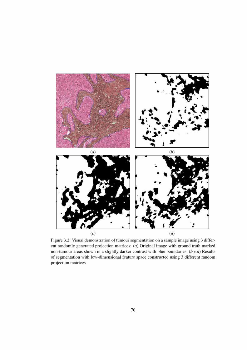
(a) (b)

(c) (d)

Figure 3.2: Visual demonstration of tumour segmentation on a sample image using 3 differ-ent randomly generated projection matrices: (a) Original image with ground truth markednon-tumour areas shown in a slightly darker contrast with blue boundaries; (b,c,d) Resultsof segmentation with low-dimensional feature space constructed using 3 different randomprojection matrices.

70

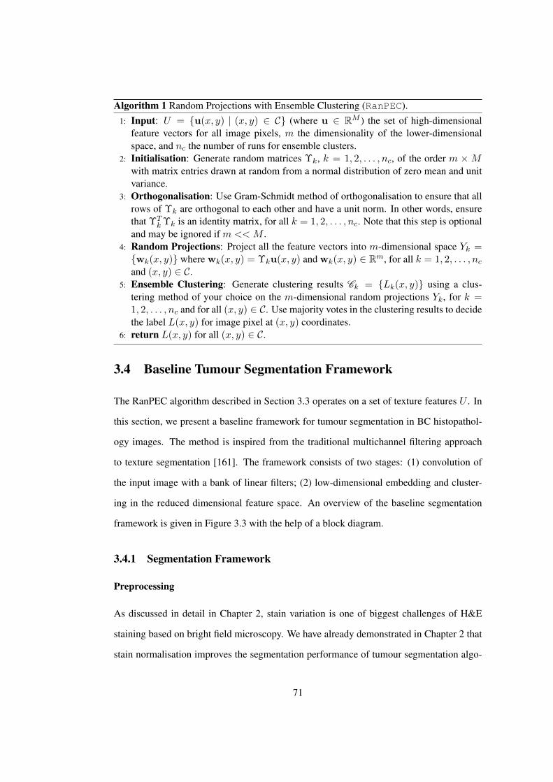
Algorithm 1 Random Projections with Ensemble Clustering (RanPEC).1: Input: U = {u(x, y) | (x, y) ∈ C} (where u ∈ RM ) the set of high-dimensional

feature vectors for all image pixels, m the dimensionality of the lower-dimensionalspace, and nc the number of runs for ensemble clusters.

2: Initialisation: Generate random matrices Υk, k = 1, 2, . . . , nc, of the order m ×Mwith matrix entries drawn at random from a normal distribution of zero mean and unitvariance.

3: Orthogonalisation: Use Gram-Schmidt method of orthogonalisation to ensure that allrows of Υk are orthogonal to each other and have a unit norm. In other words, ensurethat ΥT

k Υk is an identity matrix, for all k = 1, 2, . . . , nc. Note that this step is optionaland may be ignored if m << M .

4: Random Projections: Project all the feature vectors into m-dimensional space Yk ={wk(x, y)} where wk(x, y) = Υku(x, y) and wk(x, y) ∈ Rm, for all k = 1, 2, . . . , ncand (x, y) ∈ C.

5: Ensemble Clustering: Generate clustering results Ck = {Lk(x, y)} using a clus-tering method of your choice on the m-dimensional random projections Yk, for k =1, 2, . . . , nc and for all (x, y) ∈ C. Use majority votes in the clustering results to decidethe label L(x, y) for image pixel at (x, y) coordinates.

6: return L(x, y) for all (x, y) ∈ C.

3.4 Baseline Tumour Segmentation Framework

The RanPEC algorithm described in Section 3.3 operates on a set of texture features U . In

this section, we present a baseline framework for tumour segmentation in BC histopathol-

ogy images. The method is inspired from the traditional multichannel filtering approach

to texture segmentation [161]. The framework consists of two stages: (1) convolution of

the input image with a bank of linear filters; (2) low-dimensional embedding and cluster-

ing in the reduced dimensional feature space. An overview of the baseline segmentation

framework is given in Figure 3.3 with the help of a block diagram.

3.4.1 Segmentation Framework

Preprocessing

As discussed in detail in Chapter 2, stain variation is one of biggest challenges of H&E

staining based on bright field microscopy. We have already demonstrated in Chapter 2 that

stain normalisation improves the segmentation performance of tumour segmentation algo-

71

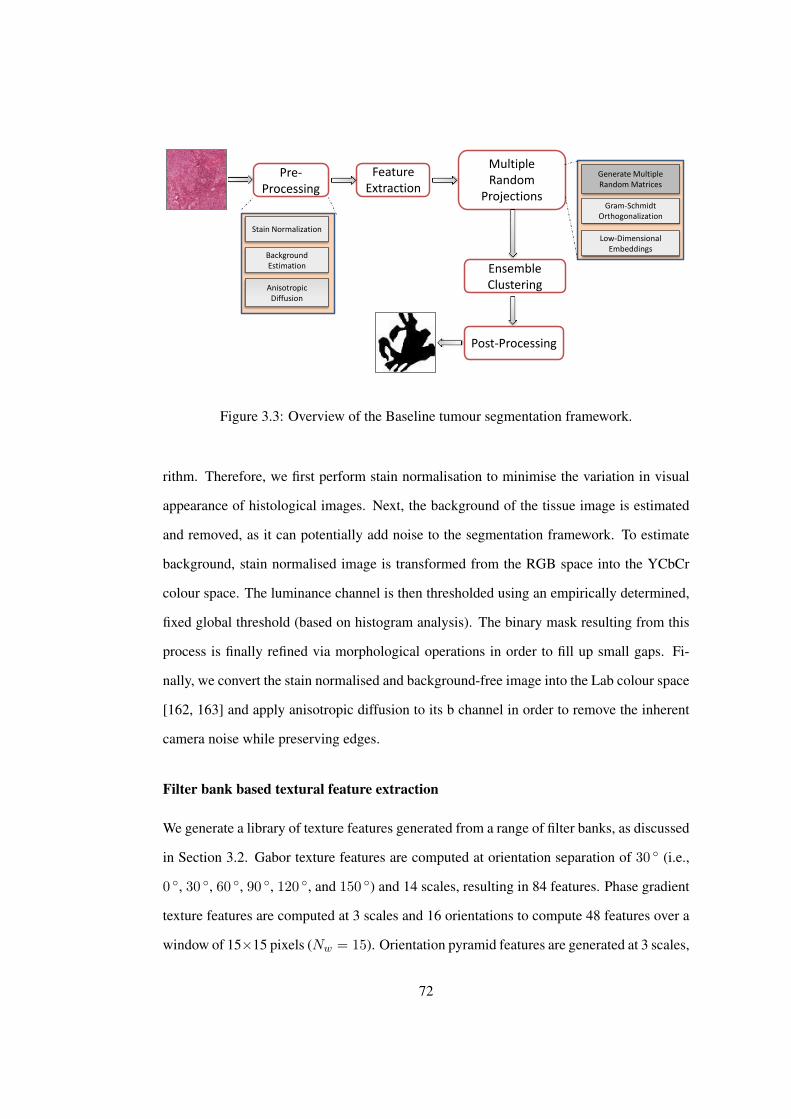
Pre-Processing

Stain Normalization

Generate Multiple Random Matrices

Anisotropic Diffusion

Gram-Schmidt Orthogonalization

Background Estimation

Post-Processing

Feature Extraction

Multiple Random

Projections

Ensemble Clustering

Low-Dimensional Embeddings

Figure 3.3: Overview of the Baseline tumour segmentation framework.

rithm. Therefore, we first perform stain normalisation to minimise the variation in visual

appearance of histological images. Next, the background of the tissue image is estimated

and removed, as it can potentially add noise to the segmentation framework. To estimate

background, stain normalised image is transformed from the RGB space into the YCbCr

colour space. The luminance channel is then thresholded using an empirically determined,

fixed global threshold (based on histogram analysis). The binary mask resulting from this

process is finally refined via morphological operations in order to fill up small gaps. Fi-

nally, we convert the stain normalised and background-free image into the Lab colour space

[162, 163] and apply anisotropic diffusion to its b channel in order to remove the inherent

camera noise while preserving edges.

Filter bank based textural feature extraction

We generate a library of texture features generated from a range of filter banks, as discussed

in Section 3.2. Gabor texture features are computed at orientation separation of 30 ◦ (i.e.,

0 ◦, 30 ◦, 60 ◦, 90 ◦, 120 ◦, and 150 ◦) and 14 scales, resulting in 84 features. Phase gradient

texture features are computed at 3 scales and 16 orientations to compute 48 features over a

window of 15×15 pixels (Nw = 15). Orientation pyramid features are generated at 3 scales,

72

resulting in 21 features. Full wavelet packet features are computed at 3 scales, generating

64 features. Spatial location features (x, y) | (x, y) ∈ C}, specifying x and y location of the

pixel on the grid with respect to the grid size are also used, as they help qualitatively improve

the performance of the segmentation algorithm in spatial neighbourhood. This generates a

84 + 48 + 21 + 64 + 2 = 219-dimensional feature vector U per pixel, which are used

in RanPEC framework to delineate the boundary of tumour regions in BC histopathology

images.

Low-dimensional embedding & clustering

In order to perform segmentation based on texture features generated in previous step,

we first perform low-dimensional embedding followed by segmentation using any unsu-

pervised clustering algorithm (e.g. k-means clustering [164]) in the reduced dimensional

feature space. For low-dimensional embedding, we compare the performance of RanPEC

framework with a widely used information theoretic feature selection algorithm, mRMR

[116]. Here we briefly describe the mRMR feature selection framework.

Minimum Redundancy Maximum Relevance: The mRMR feature selection

method employs mutual information (MI), an information theoretic measure, to select a

subset of best discriminatory features that maximise the accuracy of a classification system

by removing redundant and irrelevant features from the data [116, 165].

Given a training data X with M features, X = {xi, i = 1, . . . ,M} and target class

labels l (e.g. tumour, stroma), feature selection problem is to find from M -dimensional

feature space X ∈ RM , a subspace of m features, that optimally characterise l. Selection

of features in mRMR framework is performed based on two criteria: minimum redundancy

(R) and maximum relevance (D). The relevance of features is maximised using,

max D =1

|X|∑

xa∈XMI(xa, l) (3.12)

73

where |.| is the cardinality of the set, and MI can be computed as,

MI(X, l) = E(X)− E (X|l) (3.13)

where E(X) is marginal entropy, given by,

E(X) = −∑

xa∈XP (xa) log2 (P (xa)) (3.14)

and E (X|l) is conditional entropy, given by,

E (X|l) = −∑

xa∈XP (xa, l) log2 (P (xa|l)) (3.15)

xa refers to the a-th feature. P (xa) is the probability density function of xa and (P (xa|l))

is the conditional density of xa given l. The redundancy R is measured by an average of

MI between each pair of features,

min R =1

|X|2∑

xa,xb∈XMI(xa, xb) (3.16)

The two constraints in (3.12) and (3.16) are combined by optimiseD andR simultaneously

using,

max f(D,R),f = D −R (3.17)

Suppose we already have a set of m − 1 features Sm−1, feature selection task will be to

select the m-th feature from the set X − Sm−1 that maximise (3.17).

Postprocessing

Postprocessing is performed on clustering results to eliminate spurious regions and also to

merge closely located clusters into larger clusters, producing relatively smooth segmenta-

tion results. This is achieved by filling the small holes (using a morphological hole filling

operator) that can result in both tumour and stromal regions as a result of unsupervised

74

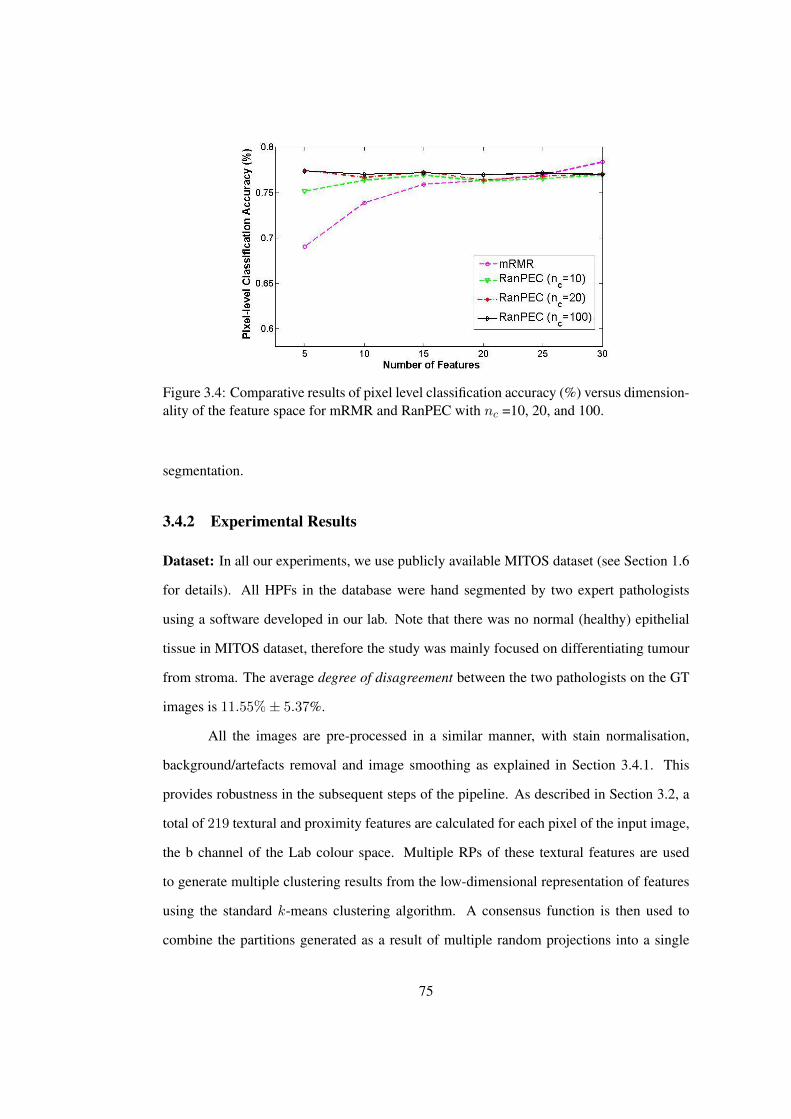
Figure 3.4: Comparative results of pixel level classification accuracy (%) versus dimension-ality of the feature space for mRMR and RanPEC with nc =10, 20, and 100.

segmentation.

3.4.2 Experimental Results

Dataset: In all our experiments, we use publicly available MITOS dataset (see Section 1.6

for details). All HPFs in the database were hand segmented by two expert pathologists

using a software developed in our lab. Note that there was no normal (healthy) epithelial

tissue in MITOS dataset, therefore the study was mainly focused on differentiating tumour

from stroma. The average degree of disagreement between the two pathologists on the GT

images is 11.55%± 5.37%.

All the images are pre-processed in a similar manner, with stain normalisation,

background/artefacts removal and image smoothing as explained in Section 3.4.1. This

provides robustness in the subsequent steps of the pipeline. As described in Section 3.2, a

total of 219 textural and proximity features are calculated for each pixel of the input image,

the b channel of the Lab colour space. Multiple RPs of these textural features are used

to generate multiple clustering results from the low-dimensional representation of features

using the standard k-means clustering algorithm. A consensus function is then used to

combine the partitions generated as a result of multiple random projections into a single

75

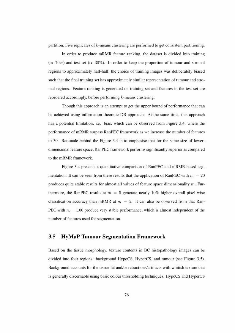
partition. Five replicates of k-means clustering are performed to get consistent partitioning.

In order to produce mRMR feature ranking, the dataset is divided into training

(≈ 70%) and test set (≈ 30%). In order to keep the proportion of tumour and stromal

regions to approximately half-half, the choice of training images was deliberately biased

such that the final training set has approximately similar representation of tumour and stro-

mal regions. Feature ranking is generated on training set and features in the test set are

reordered accordingly, before performing k-means clustering.

Though this approach is an attempt to get the upper bound of performance that can

be achieved using information theoretic DR approach. At the same time, this approach

has a potential limitation, i.e. bias, which can be observed from Figure 3.4, where the

performance of mRMR surpass RanPEC framework as we increase the number of features

to 30. Rationale behind the Figure 3.4 is to emphasise that for the same size of lower-

dimensional feature space, RanPEC framework performs significantly superior as compared

to the mRMR framework.

Figure 3.4 presents a quantitative comparison of RanPEC and mRMR based seg-

mentation. It can be seen from these results that the application of RanPEC with nc = 20

produces quite stable results for almost all values of feature space dimensionality m. Fur-

thermore, the RanPEC results at m = 5 generate nearly 10% higher overall pixel wise

classification accuracy than mRMR at m = 5. It can also be observed from that Ran-

PEC with nc = 100 produce very stable performance, which is almost independent of the

number of features used for segmentation.

3.5 HyMaP Tumour Segmentation Framework

Based on the tissue morphology, texture contents in BC histopathology images can be

divided into four regions: background HypoCS, HyperCS, and tumour (see Figure 3.5).

Background accounts for the tissue fat and/or retractions/artifacts with whitish texture that

is generally discernable using basic colour thresholding techniques. HypoCS and HyperCS

76

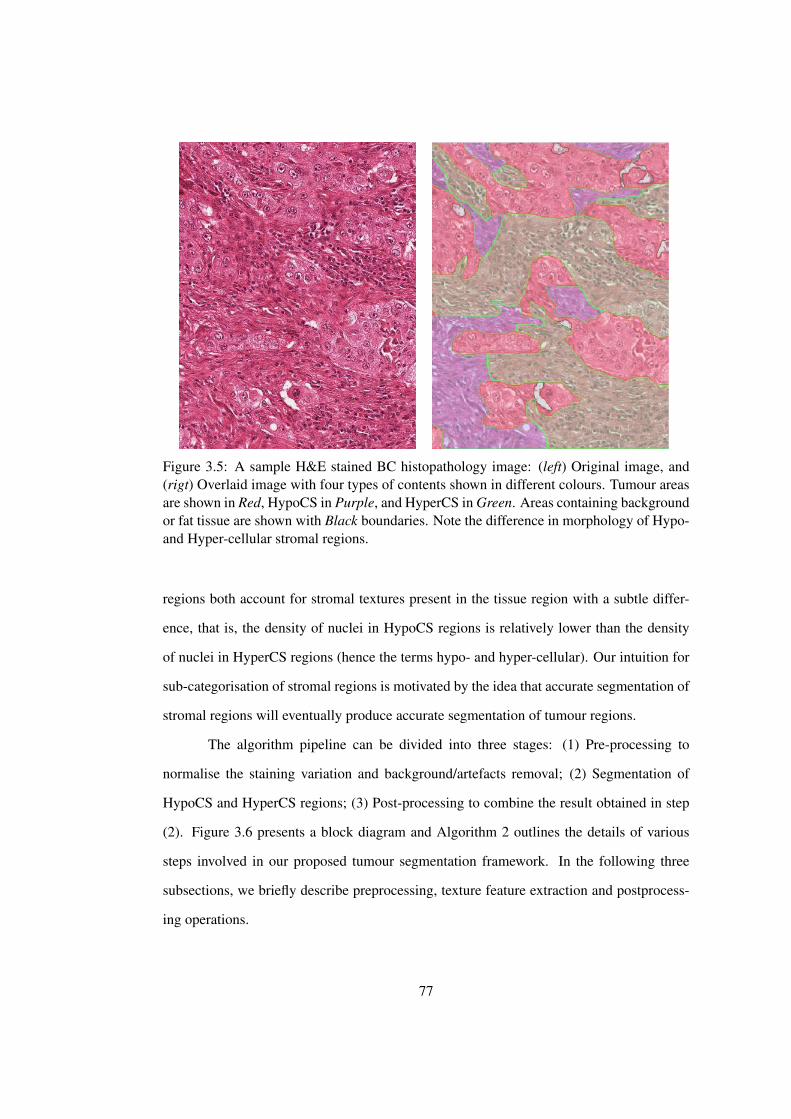
Figure 3.5: A sample H&E stained BC histopathology image: (left) Original image, and(rigt) Overlaid image with four types of contents shown in different colours. Tumour areasare shown in Red, HypoCS in Purple, and HyperCS in Green. Areas containing backgroundor fat tissue are shown with Black boundaries. Note the difference in morphology of Hypo-and Hyper-cellular stromal regions.

regions both account for stromal textures present in the tissue region with a subtle differ-

ence, that is, the density of nuclei in HypoCS regions is relatively lower than the density

of nuclei in HyperCS regions (hence the terms hypo- and hyper-cellular). Our intuition for

sub-categorisation of stromal regions is motivated by the idea that accurate segmentation of

stromal regions will eventually produce accurate segmentation of tumour regions.

The algorithm pipeline can be divided into three stages: (1) Pre-processing to

normalise the staining variation and background/artefacts removal; (2) Segmentation of

HypoCS and HyperCS regions; (3) Post-processing to combine the result obtained in step

(2). Figure 3.6 presents a block diagram and Algorithm 2 outlines the details of various

steps involved in our proposed tumour segmentation framework. In the following three

subsections, we briefly describe preprocessing, texture feature extraction and postprocess-

ing operations.

77

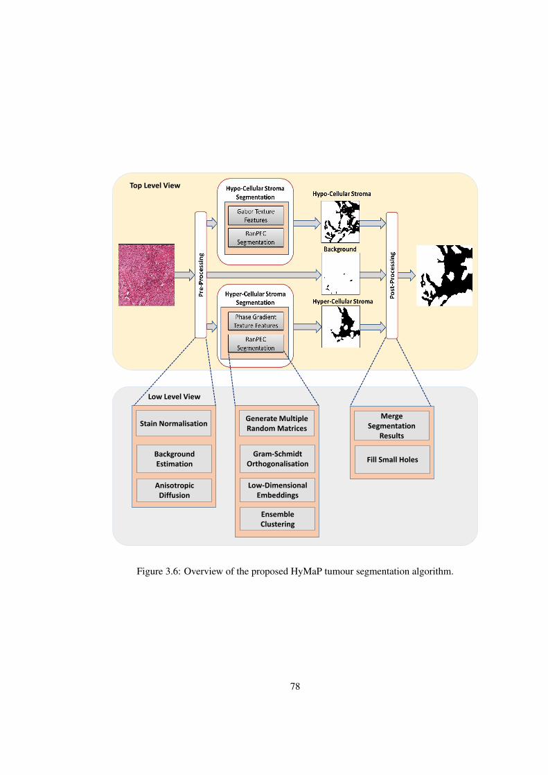
Top Level View

Low Level View

Stain Normalisation

Anisotropic Diffusion

Background Estimation

Merge Segmentation

Results

Fill Small Holes

Generate Multiple Random Matrices

Low-Dimensional Embeddings

Gram-Schmidt Orthogonalisation

Ensemble Clustering

Figure 3.6: Overview of the proposed HyMaP tumour segmentation algorithm.

78

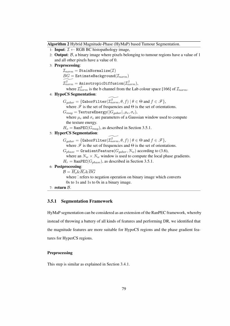
Algorithm 2 Hybrid Magnitude-Phase (HyMaP) based Tumour Segmentation.1: Input: I ← RGB BC histopathology image,2: Output: B, a binary image where pixels belonging to tumour regions have a value of 1

and all other pixels have a value of 0.3: Preprocessing:

Inorm = StainNormalize(I)BG = EstimateBackground(Inorm)

Iβnorm = AnisotropicDiffusion(Iβnorm),where Iβnorm is the b channel from the Lab colour space [166] of Inorm.

4: HypoCS Segmentation:

Ggabor = {GaborFilter(Iβnorm, θ, f) | θ ∈ Θ and f ∈ F},where F is the set of frequencies and Θ is the set of orientations.

Gmag = TextureEnergy(|Ggabor|, µe, σe),where µe and σe are parameters of a Gaussian window used to computethe texture energy.

Ho = RanPEC(Gmag), as described in Section 3.5.1.5: HyperCS Segmentation:

Ggabor = {GaborFilter(Iβnorm, θ, f) | θ ∈ Θ and f ∈ F},where F is the set of frequencies and Θ is the set of orientations.

Gphase = GradientFeature(Ggabor, Nw) according to (3.6),where an Nw ×Nw window is used to compute the local phase gradients.

Hr = RanPEC(Gphase), as described in Section 3.5.1.6: Postprocessing:

B = Ho&Hr&BGwhere . refers to negation operation on binary image which converts0s to 1s and 1s to 0s in a binary image.

7: return B.

3.5.1 Segmentation Framework

HyMaP segmentation can be considered as an extension of the RanPEC framework, whereby

instead of throwing a battery of all kinds of features and performing DR, we identified that

the magnitude features are more suitable for HypoCS regions and the phase gradient fea-

tures for HyperCS regions.

Preprocessing

This step is similar as explained in Section 3.4.1.

79

Hypo- and Hyper-Cellular Stromal Segmentation

In Section 3.4, we presented baseline tumour segmentation framework, where we employed

a dictionary of texture features that were derived from four filter banks; Gabor, phase gra-

dient, orientation pyramid and wavelet packet transform. The intuition was to separate

the tumour regions from stroma using a multichannel texture representation. In HyMaP

however, we are interested in modelling the texture of two stromal sub-types, HypoCS and

HyperCS. Therefore, our approach is to evaluate various filter bank based representations of

the two sub-stromal regions and find an optimal set of filters that facilitate the segmentation

of the two sub-stromal regions in BC histopathology images.

We investigated the magnitude and phase spectra of the Gabor filter bank and found

it to be effective in segmenting the two sub-categories of stromal textures, respectively.

Step 4 and 5 in Algorithm 2 present the sequence of operations performed during HypoCS

and HyperCS segmentations. In step 4, a preprocessed image is first convolved with a bank

of Gabor filters. Each filtered image is subjected to a nonlinear transformation (sigmoidal

function), to avoid homogeneity that might arise if spatial pooling, i.e., spatial averaging

over a region greater than the area of a micropattern, is performed [161]. This means

that the positive and negative parts of the response on each micropattern may have the

same average and thus the pooled responses may not be directly useful to discriminate the

two micropatterns (see Figure 4 in [161]). Energy is computed in terms of square of each

coefficient of all Gabor responses. RanPEC framework is then used to obtain HypoCS

segmentation. In step 5, each preprocessed image is first convolved with a bank of Gabor

filters. Phase gradient features are computed in a small neighbourhood using the procedure

outlined in Section 3.2.2. Finally, RanPEC framework is employed to generate HyperCS

segmentation.

HypoCS regions are mostly composed of connective tissues, which are generally

smooth textures with few lymphocytes or fibroblasts. HyperCS regions on the other hand,

are infiltrated by large number of cells and the texture of such regions is relative rough. Note

that, the two segmentations are complementary, not mutually exclusive which is expected as

80

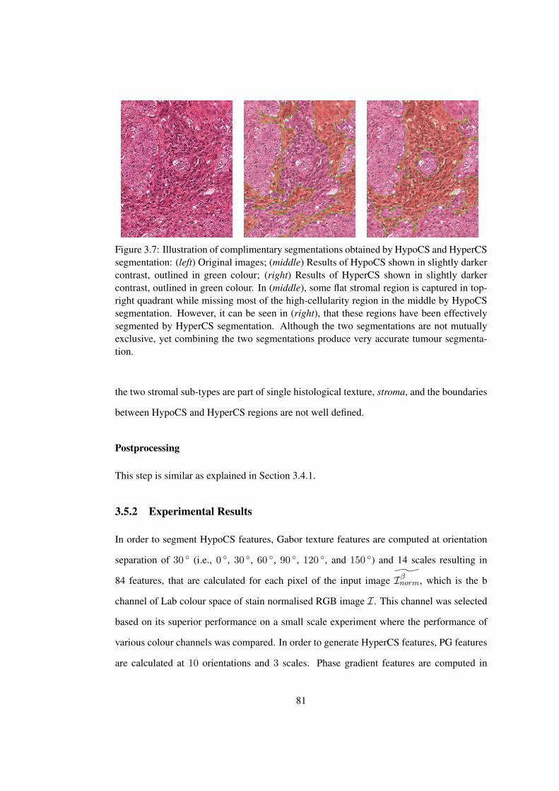
Figure 3.7: Illustration of complimentary segmentations obtained by HypoCS and HyperCSsegmentation: (left) Original images; (middle) Results of HypoCS shown in slightly darkercontrast, outlined in green colour; (right) Results of HyperCS shown in slightly darkercontrast, outlined in green colour. In (middle), some flat stromal region is captured in top-right quadrant while missing most of the high-cellularity region in the middle by HypoCSsegmentation. However, it can be seen in (right), that these regions have been effectivelysegmented by HyperCS segmentation. Although the two segmentations are not mutuallyexclusive, yet combining the two segmentations produce very accurate tumour segmenta-tion.

the two stromal sub-types are part of single histological texture, stroma, and the boundaries

between HypoCS and HyperCS regions are not well defined.

Postprocessing

This step is similar as explained in Section 3.4.1.

3.5.2 Experimental Results

In order to segment HypoCS features, Gabor texture features are computed at orientation

separation of 30 ◦ (i.e., 0 ◦, 30 ◦, 60 ◦, 90 ◦, 120 ◦, and 150 ◦) and 14 scales resulting in

84 features, that are calculated for each pixel of the input image Iβnorm, which is the b

channel of Lab colour space of stain normalised RGB image I. This channel was selected

based on its superior performance on a small scale experiment where the performance of

various colour channels was compared. In order to generate HyperCS features, PG features

are calculated at 10 orientations and 3 scales. Phase gradient features are computed in

81

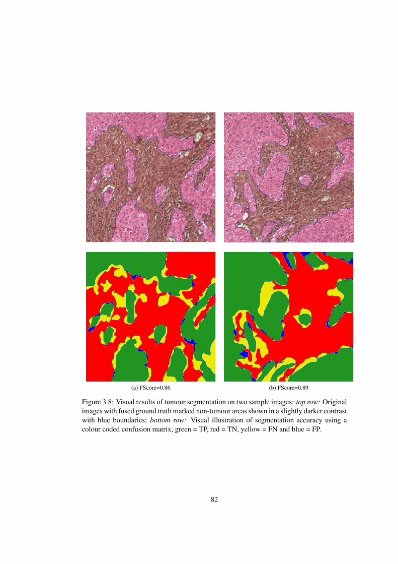
(a) FScore=0.86 (b) FScore=0.89

Figure 3.8: Visual results of tumour segmentation on two sample images: top row: Originalimages with fused ground truth marked non-tumour areas shown in a slightly darker contrastwith blue boundaries; bottom row: Visual illustration of segmentation accuracy using acolour coded confusion matrix, green = TP, red = TN, yellow = FN and blue = FP.

82

a window of size 15 × 15 (Nw = 15). RanPEC segmentation framework is applied on

both Gabor and PG features independently yielding HypoCS and HyperCS segmentations

respectively. RanPEC framework require 2 parameters: m the dimensionality of lower

dimensional space, and nc the number of runs of ensemble. As shown in previous section,

we used m = 5 and nc = 20 in our experiments as they yield stable results. We compare

the tumour segmentation accuracy of the proposed algorithm (HyMaP) with the baseline

using the same experimental setup as presented in the previous section.

The algorithms are evaluated on three pixel-wise accuracy measures: precision,

recall, and F1-Score. F1-Score is a measure that combines precision and recall in a statisti-

cally more meaningful way. Let TP denotes the number of true positive, FP the number of

false positive, TN the number of true negatives, and FN the number of false negatives, pre-

cision is defined as TP/(TP+FP), recall is defined as TP/(TP+FN) and F1-Score is defined

as 2×(precision×recall)/(precision + recall). We generate experimental results on 3 crite-

ria: (1) considering pathologist-1’s markings (P-1) as GT; (2) considering pathologist-2’s

markings (P-2) as GT; (3) fusing P-1 and P-2 using logical OR rule (i.e. a pixel is consid-

ered to be tumourous if any one of the two pathologists marked the pixel as tumourous),

and considering the fused image as GT. Some of HPF images contain large tumour regions

with small islands of stroma here and there, however majority of HPF images contain a fair

share of stroma regions (approx. 33%, on average).

Figure 3.7 provides illustration of the efficiency of HypoCS segmentation [Figure

3.7(b)] and HyperCS segmentation [Figure 3.7(c)] in capturing complimentary stromal sub-

types. Note that the two segmentations are complementary, not mutually exclusive, however

the combination of the two segmentations delineates accurate tumour segmentation. Figure

3.8 provides illustration of the proposed tumour segmentation algorithm on 2 different HPF

images. Segmentation results obtained by combining HypoCS and HyperCS yield high F1-

Score of 0.86 and 0.89 with respect to the fused GT. Considering the degree of agreement

between the two pathologists (i.e. 92.41% ± 3.49% in terms of F1-Score), the results can

be termed as relatively accurate.

83

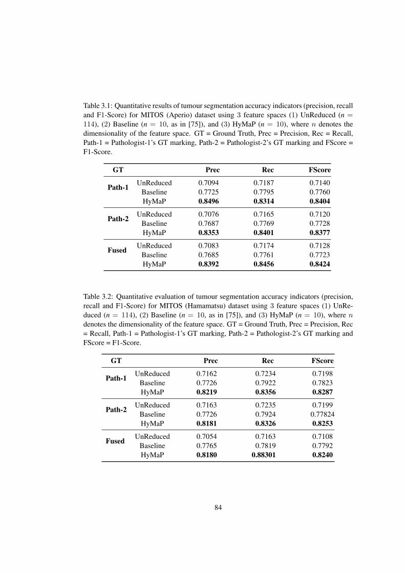
Table 3.1: Quantitative results of tumour segmentation accuracy indicators (precision, recalland F1-Score) for MITOS (Aperio) dataset using 3 feature spaces (1) UnReduced (n =114), (2) Baseline (n = 10, as in [75]), and (3) HyMaP (n = 10), where n denotes thedimensionality of the feature space. GT = Ground Truth, Prec = Precision, Rec = Recall,Path-1 = Pathologist-1’s GT marking, Path-2 = Pathologist-2’s GT marking and FScore =F1-Score.

GT Prec Rec FScore

Path-1 UnReduced 0.7094 0.7187 0.7140Baseline 0.7725 0.7795 0.7760HyMaP 0.8496 0.8314 0.8404

Path-2 UnReduced 0.7076 0.7165 0.7120Baseline 0.7687 0.7769 0.7728HyMaP 0.8353 0.8401 0.8377

Fused UnReduced 0.7083 0.7174 0.7128Baseline 0.7685 0.7761 0.7723HyMaP 0.8392 0.8456 0.8424

Table 3.2: Quantitative evaluation of tumour segmentation accuracy indicators (precision,recall and F1-Score) for MITOS (Hamamatsu) dataset using 3 feature spaces (1) UnRe-duced (n = 114), (2) Baseline (n = 10, as in [75]), and (3) HyMaP (n = 10), where ndenotes the dimensionality of the feature space. GT = Ground Truth, Prec = Precision, Rec= Recall, Path-1 = Pathologist-1’s GT marking, Path-2 = Pathologist-2’s GT marking andFScore = F1-Score.

GT Prec Rec FScore

Path-1 UnReduced 0.7162 0.7234 0.7198Baseline 0.7726 0.7922 0.7823HyMaP 0.8219 0.8356 0.8287

Path-2 UnReduced 0.7163 0.7235 0.7199Baseline 0.7726 0.7924 0.77824HyMaP 0.8181 0.8326 0.8253

Fused UnReduced 0.7054 0.7163 0.7108Baseline 0.7765 0.7819 0.7792HyMaP 0.8180 0.88301 0.8240

84

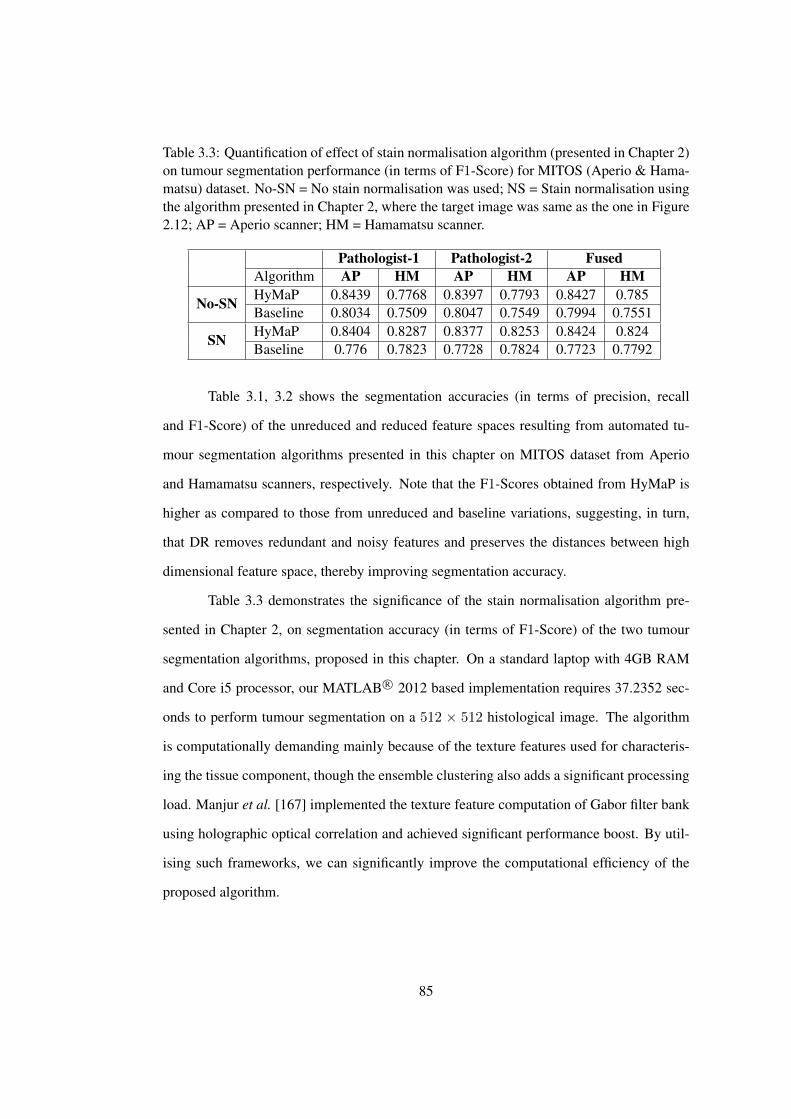
Table 3.3: Quantification of effect of stain normalisation algorithm (presented in Chapter 2)on tumour segmentation performance (in terms of F1-Score) for MITOS (Aperio & Hama-matsu) dataset. No-SN = No stain normalisation was used; NS = Stain normalisation usingthe algorithm presented in Chapter 2, where the target image was same as the one in Figure2.12; AP = Aperio scanner; HM = Hamamatsu scanner.

Pathologist-1 Pathologist-2 FusedAlgorithm AP HM AP HM AP HM

No-SN HyMaP 0.8439 0.7768 0.8397 0.7793 0.8427 0.785Baseline 0.8034 0.7509 0.8047 0.7549 0.7994 0.7551

SN HyMaP 0.8404 0.8287 0.8377 0.8253 0.8424 0.824Baseline 0.776 0.7823 0.7728 0.7824 0.7723 0.7792

Table 3.1, 3.2 shows the segmentation accuracies (in terms of precision, recall

and F1-Score) of the unreduced and reduced feature spaces resulting from automated tu-

mour segmentation algorithms presented in this chapter on MITOS dataset from Aperio

and Hamamatsu scanners, respectively. Note that the F1-Scores obtained from HyMaP is

higher as compared to those from unreduced and baseline variations, suggesting, in turn,

that DR removes redundant and noisy features and preserves the distances between high

dimensional feature space, thereby improving segmentation accuracy.

Table 3.3 demonstrates the significance of the stain normalisation algorithm pre-

sented in Chapter 2, on segmentation accuracy (in terms of F1-Score) of the two tumour

segmentation algorithms, proposed in this chapter. On a standard laptop with 4GB RAM

and Core i5 processor, our MATLAB R© 2012 based implementation requires 37.2352 sec-

onds to perform tumour segmentation on a 512 × 512 histological image. The algorithm

is computationally demanding mainly because of the texture features used for characteris-

ing the tissue component, though the ensemble clustering also adds a significant processing

load. Manjur et al. [167] implemented the texture feature computation of Gabor filter bank

using holographic optical correlation and achieved significant performance boost. By util-

ising such frameworks, we can significantly improve the computational efficiency of the

proposed algorithm.

85

3.6 Summary

In this chapter, we addressed the issue of robustness of clustering results in the context of

RPs. We proposed RanPEC framework that addresses this issue by combining clustering re-

sults from multiple RPs using a majority vote. We demonstrated that the proposed RanPEC

framework preserves the Euclidean distance between points in high-dimensional spaces in

a robust manner. Utilising the RanPEC framework, we further presented an algorithm for

segmentation of tumour areas in BC histopathology images. The algorithm characterises a

stromal texture in BC histological images into HypoCS and HyperCS regions using mag-

nitude and phase spectra respectively, in the Gabor domain. We demonstrated that the two

spectra provide complimentary segmentation of hypo- and hyper-cellular stromal regions

with high degree of segmentation accuracy as compared to GT marked by two pathologists.

86

Chapter 4

Mitotic Cell Detection

Detection and segmentation of cells in histopathology images is a subject of interest in a

wide range of cell-based studies as it is critical for evaluating the existence of disease and

its severity. For example, infiltration of lymphocytes in BC has been shown to be related to

patient survival [168]. Similarly, nuclear atypia has diagnostic value for cancer grading [25,

169] and mitotic count is an important prognostic parameter in BC grading [170]. However,

it is a very challenging problem, especially for H&E stained histological sections. Two main

factors that make it a challenging problem are: (1) variation due to staining which may leave

some of the nuclei weakly stained. Thus, a histological image might have large number of

nuclei with broken cell membrane making them difficult to discern from the background

texture; (2) diversity in the shape of epithelial cancerous nuclei, whose appearance may

vary from a round normal nucleus to an enlarged and irregularly deformed nucleus with

scrambled chromatin structures. The difficulty of the problem increases significantly when

the cell density of tissue sample is high, resulting in cell overlap and clumping issues.

4.1 Related Work

There are two aspects of cell segmentation: detection and segmentation.

88

4.1.1 Cell Detection

For cell detection, a variety of methods have been proposed in the literature [171, 172, 173,

174]. Thresholding based approaches use adaptive threshold [175], fuzzy c-means cluster-

ing [176] or expectation maximisation (EM) algorithm [177] to detect nuclei. However,

these approaches generally work only if the cells are well defined and background is uni-

form, which rarely occurs in the case of histological images. Blob detection approaches use

Laplacian of Gaussian [178], difference of Gaussians [179], h-maxima transform [180] or

h-minima transform [181] to detect cells. These methods are based on the assumption that

the morphological properties of the region, or blob, are constant or varying within a small

range of values. The assumption generally doesn’t hold well in case of nuclei in H&E

stained images which may be highly textured. Additionally, nuclei in high grade tumours

do not usually have constant morphological properties within the cellular regions, which

severely hampers the performance of such algorithms.

In Hough transform based cell detection methods [182], a parametric model is used

to detect the pixel locations belonging to a cell. In addition to being computationally de-

manding, such approaches fail because of highly textured nature of some nuclei in his-

tological images which makes the edge map extremely noisy for Hough transform based

algorithms. Secondly, cancerous nuclei generally do not follow any regular shape, which

makes hough transform based approaches less suitable choice for histopathology images.

Radial symmetry [183], which determines the contribution each pixel makes to-

wards the symmetry of the pixels around it, has been used by some researchers to detect

nuclei in histopathology images [184]. Similarly, Kuse et al. [77] quantify the symmetry

around a pixel to detect nuclei. They specifically exploit some nice properties of frequency

domain, like invariance to contrast and illumination, while measuring symmetry. A similar

approach is proposed in [185] and [186] where a set of specifically designed shifted Gaus-

sian kernels, amplifying the voting at the center of the cell, is employed to perform cell

detection.

Vink et al. [181] employ a machine learning strategy, because of the ability of ma-

89

chine learning methods to generalise complex objects (e.g. faces) [187]. They learn two

Adaboost based detectors: (1) a pixel based detector that generalises the internal structure of

nuclei; (2) a line based detector that characterises the boundary structure of nuclei. The two

detections are performed in hematoxylin channel, which is obtained using CD framework

[73]. The results of the two detections are combined in postprocessing step to generate final

detections.

Some methods employ two step processing to identify candidate cells. In the first

step, a large set of candidate cells is identified. In the second step, a subset of these can-

didates is chosen based on their fitness to some predefined criterion. In [188], candidate

cells are efficiently identified by the maximally stable extremal regions detector [189]. This

detector produces a large number of potentially overlapping regions. Fitness of each candi-

date region is evaluated using a statistical model, and dynamic programming is employed to

select an optimal set of non-overlapping regions that best fit the model. Wienert et al. [190]

employ contour tracing approach [191] to detect cells in histological images. Using this

approach, contour of an object is followed in clockwise direction using 8-connected neigh-

bourhood grid. A contour is considered valid only if it ends at the same pixel where it

started. The contours generated using this procedure often have overlapping areas, many of

which do not represent the actual nuclei. Thus, the contour tracing procedure is followed

by contour evaluation procedure, which removes some of the over-defined cells.

4.1.2 Cell Segmentation

Cell segmentation methods can be broadly divided into five main categories [171, 172, 173,

174]: Intensity based, region based, active contours/level sets, probabilistic and graphical

models. Intensity based methods (e.g. thresholding) search for optimal value of intensity

(in both greyscale [175, 192, 193] and colour channels [194]) such that the intensities that

belong to the cells are separated from the intensities that belong to the background. Intensity

based methods are computationally efficient, but generally demonstrate poor segmentation

performance since they only use pixel level information and ignore wealth of information

90

at the object level.

Region based methods (e.g. watershed, region growing) generally work on the in-

tensity values as well, however they follow the basic principle of merging two neighbouring

regions if the regions satisfy some predefined merging criterion [195]. Several algorithms

employ watershed algorithm for cell segmentation in histological images [184, 196, 197].

A major advantage of using the watershed algorithm, in particular, is that it does not re-

quire parameter tuning. However, it requires the initial set of seed points. Therefore, these

algorithms are generally combined with one of the detection methods described above. For

instance, Veta et al. [184] use radial symmetry transform to detect seeds followed by marker

controlled watershed transform to segment nuclei.

Active contour models [198, 199, 200] are deformable splines that can be used to

depict the contour of nuclei based on gradient information. Such models are very effective

in combining object level information (e.g. shape) with pixel level information (e.g. image

gradients, edges and colour distributions). Like watershed based methods, active contour

models also require initial set of seed points. Therefore, they are generally used in com-

bination with one of the cell detection algorithms [177, 179, 201, 202, 203]. Cosatto et

al. [179] employ a combination of difference of Gaussians and Hough transform to detect

candidate nuclei followed by active contour to perform segmentation. Irshad et al. [202]

and Veta et al. [203] perform mitotic cell detection using intensity thresholding followed

by cell boundary delineation using active contour model.

Probabilistic models (e.g. GMM) represent cells in histopathology images as weighted

sum of several Gaussian densities or as a mixture of Gaussian and other (e.g. Gamma) den-

sities [37, 181]. The parameters for these models are usually estimated from training data

using parameter estimation techniques such as EM [204].

Graphical models (e.g. graph cut [205, 206, 207]) conceptualise images as graphs,

where each pixel is represented by a node in the graph and the relationship between neigh-

bouring pixels is represented by edges. These methods partition the graph into disjoint

subgraphs such that similarity is high within the subgraphs and low across different sub-

91

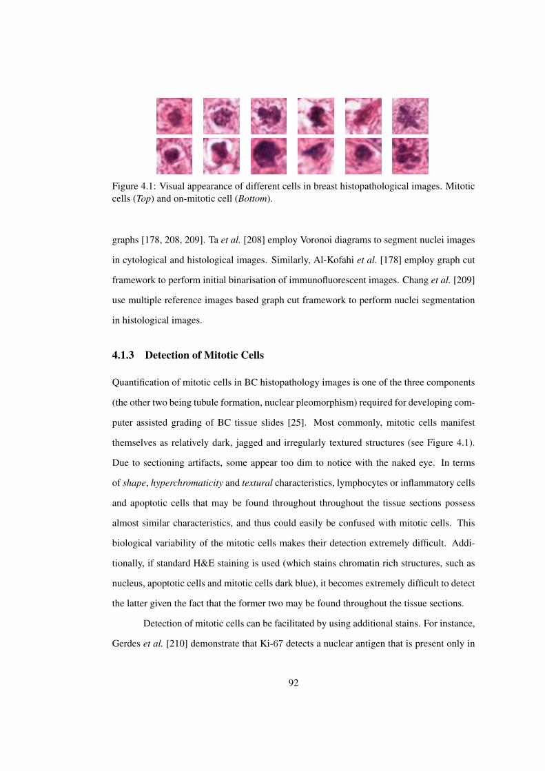
Figure 4.1: Visual appearance of different cells in breast histopathological images. Mitoticcells (Top) and on-mitotic cell (Bottom).

graphs [178, 208, 209]. Ta et al. [208] employ Voronoi diagrams to segment nuclei images

in cytological and histological images. Similarly, Al-Kofahi et al. [178] employ graph cut

framework to perform initial binarisation of immunofluorescent images. Chang et al. [209]

use multiple reference images based graph cut framework to perform nuclei segmentation

in histological images.

4.1.3 Detection of Mitotic Cells

Quantification of mitotic cells in BC histopathology images is one of the three components

(the other two being tubule formation, nuclear pleomorphism) required for developing com-

puter assisted grading of BC tissue slides [25]. Most commonly, mitotic cells manifest

themselves as relatively dark, jagged and irregularly textured structures (see Figure 4.1).

Due to sectioning artifacts, some appear too dim to notice with the naked eye. In terms

of shape, hyperchromaticity and textural characteristics, lymphocytes or inflammatory cells

and apoptotic cells that may be found throughout throughout the tissue sections possess

almost similar characteristics, and thus could easily be confused with mitotic cells. This

biological variability of the mitotic cells makes their detection extremely difficult. Addi-

tionally, if standard H&E staining is used (which stains chromatin rich structures, such as

nucleus, apoptotic cells and mitotic cells dark blue), it becomes extremely difficult to detect

the latter given the fact that the former two may be found throughout the tissue sections.

Detection of mitotic cells can be facilitated by using additional stains. For instance,

Gerdes et al. [210] demonstrate that Ki-67 detects a nuclear antigen that is present only in

92

proliferating cells. The study which was aimed to investigate the expression of Ki-67 in cell

division life cycle concluded that Ki-67 is consistently present in all phases of cell life cycle

except G0 phase (which is a phase in cell life cycle when the cell stops dividing and exists

in resting phase). Since Ki-67 is not exclusively specific to mitosis, it generally produces

higher estimates of mitotic cells when compared to H&E sections [211].

Phosphohistone H3 (PPH3) on the other hand, has the advantage of staining mi-

totic nuclei exclusively and has been demonstrated to have prognostic significance [212].

Despite these studies, IHC stains are generally not used in routine clinical practice due to

the increased cost and the time delay involved. Manual counting of mitotic cells, on the

other hand, still remains the most widely practiced method for establishing mitotic index,

and thus, there is a significant potential for developing algorithms that perform automated

counting of mitotic cells in H&E stained histological images.

The earliest approaches to mitotic cell detection either employ an additional stain,

e.g. Feulgen [213, 214, 215] or Ki-67 [216], or use a video sequence to detect mitotic events

over time by incorporating spatial and temporal information [217]. Recently, two datasets of

H&E stained BC histopathology images (MITOS [41] and Amida [218]) with GT, annotated

by the consensus of multiple expert pathologists were made publicly available. With these

public domain datasets, a number of mitotic cell detection algorithms have been recently

proposed [37, 202, 203, 219, 220, 221, 222, 223, 224, 225, 226].

Most of the computerised approaches to mitotic cell detection work by first iden-

tifying candidate objects or locations that are then accepted (or rejected) as mitotic cells

based on some similarity criterion [37, 202, 203, 219, 220, 221, 222, 223, 224, 225]. The

candidate extraction phase often makes use of the colour distinctiveness of mitotic cells by

performing pixel-wise colour classification [222] or thresholding [202, 203, 220, 225]. This

is because the intensity of mitotic cells is noticeably darker than normal epithelial nuclei and

only comparable to apoptotic, necrotic or compressed (artefact from the tissue preparation)

and lymphocyte nuclei. These local intensity minima detection methods are sometimes

followed by refinement of the detected regions by morphological operations and/or active

93

contours segmentation [202, 203]. In the second phase, features ranging from basic fea-

tures (morphological, geometrical and textural) to more specialised features (such as those

learned from deep convolutional neural networks [219, 221, 227]) are used in a classifi-

cation framework. The approach presented in [219] doesn’t employ candidate detection

phase, and trains a pixel level deep convolution network which takes all the training pixels

along with their immediate surrounding pixels as input, and builds a deep neural network

model for mitotic cells which is directly used on test data to perform classification.

4.2 Our Approach

In this chapter, we present a novel framework for mitotic cell detection in BC histopathol-

ogy images. The framework mimics a pathologist’s approach to mitotic cells detection

under the microscope. The main idea is to isolate tumour region from non-tumour regions

(consisting of lymphocytes, inflammatory, and apoptotic cells) and search for mitotic cells

in the tumour regions. Candidate mitotic cells are identified by statistically modelling the

pixel intensities in mitotic and non-mitotic regions. Candidate classification is performed

based on morphological characteristics along with the surrounding context of each candi-

date mitotic cell.

Figure 4.2 provides an overview of the proposed mitotic cell detection framework.

Essentially, there are 4 components of the proposed system: (1) stain normalisation; (2)

tumour segmentation; (3) candidate mitotic cell detection; (4) candidate classification by

modelling the visual appearance of mitotic and non-mitotic cells. The topics of stain nor-

malisation and tumour segmentation have been addressed in detail in Chapters 2 and 3,

respectively. In the next three sections, we present details of the proposed candidate cell

detection and classification frameworks.

Following list accounts for the novel contributions of this chapter:

1. We present a novel framework for detection of mitotic cells in BC histopathology

images, which mimics a pathologist’s approach to mitotic cell counting (see Figure

94

4.2).

2. We propose GGMM for detecting mitotic cells in BC histopathology images. Image

intensities are modelled as random variables sampled from one of the two distribu-

tions; Gamma and Gaussian. Intensities from mitotic cells are modelled by a Gamma

distribution and those from non-mitotic regions are modelled by a Gaussian distribu-

tion (Section 4.3).

3. We propose context, i.e. texture surrounding a cell, as a clue for classifying cells into

mitotic and non-mitotic classes (Section 4.4).

4. We employ cell words, a novel framework for modelling the visual appearance of

cells in histopathology images and apply this model to discriminate between mitotic

and non-mitotic cells.

5. We demonstrate that the proposed framework achieves high detection performance

on MITOS and WarMiCe BC histopathology image datasets (Section 4.7).

The rest of this chapter is organised as follows: Section 4.3 presents GGMM for

candidate detection. Section 4.4 presents CAPP; a feature based approach for candidate

classification of mitotic cells. Section 4.5 presents cell words framework; an appearance

based approach for classification of mitotic cells. Section 4.6 provides experimental setup

and details of various parameters used for evaluation of the proposed methods in Sections

4.3, 4.4 and 4.5. Section 4.7 presents the experimental results and discussion. Section 4.8

provides a summary of the chapter.

4.3 Gamma-Gaussian Mixture Model for Candidate Detection

We propose GGMM for candidate mitotic cell detection in BC histopathology images.

Image intensities (the L channel of Lab colour space) are modelled as random variables

sampled from one of the two distributions; Gamma and Gaussian. Intensities from mitotic

95

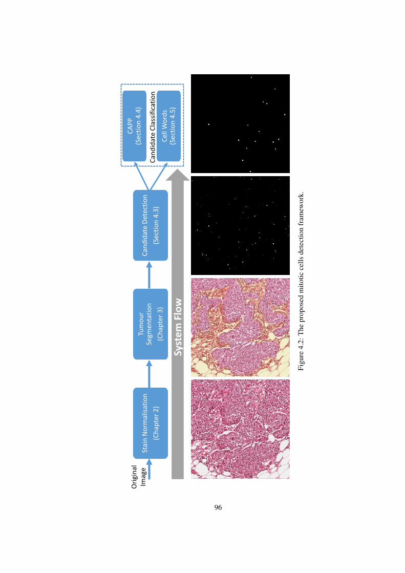
Syst

em

Flo

w

Stai

n N

orm

alis

atio

n

(Ch

apte

r 2

)

Tum

ou

rSe

gmen

tati

on

(Ch

apte

r 3

)

Can

did

ate

Det

ecti

on

(Sec

tio

n 4

.3)

Can

did

ate

Cla

ssif

icat

ion

CA

PP

(Sec

tio

n 4

.4)

Cel

l Wo

rds

(Sec

tio

n 4

.5)

Ori

gin

al

Imag

e

Figu

re4.

2:T

hepr

opos

edm

itotic

cells

dete

ctio

nfr

amew

ork.

96

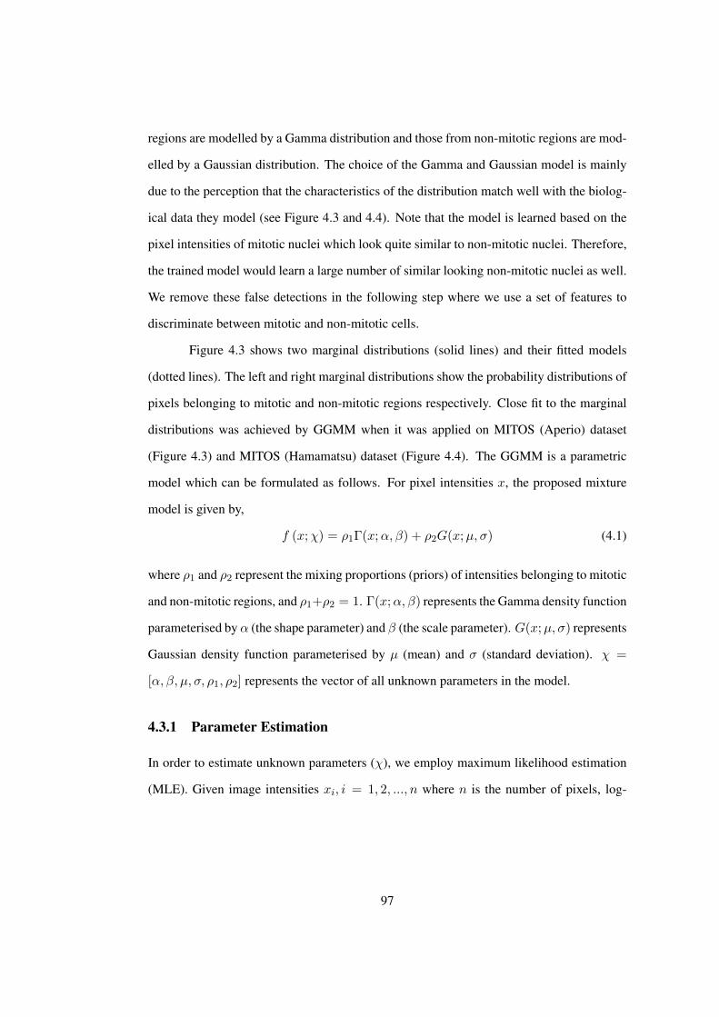
regions are modelled by a Gamma distribution and those from non-mitotic regions are mod-

elled by a Gaussian distribution. The choice of the Gamma and Gaussian model is mainly

due to the perception that the characteristics of the distribution match well with the biolog-

ical data they model (see Figure 4.3 and 4.4). Note that the model is learned based on the

pixel intensities of mitotic nuclei which look quite similar to non-mitotic nuclei. Therefore,

the trained model would learn a large number of similar looking non-mitotic nuclei as well.

We remove these false detections in the following step where we use a set of features to

discriminate between mitotic and non-mitotic cells.

Figure 4.3 shows two marginal distributions (solid lines) and their fitted models

(dotted lines). The left and right marginal distributions show the probability distributions of

pixels belonging to mitotic and non-mitotic regions respectively. Close fit to the marginal

distributions was achieved by GGMM when it was applied on MITOS (Aperio) dataset

(Figure 4.3) and MITOS (Hamamatsu) dataset (Figure 4.4). The GGMM is a parametric

model which can be formulated as follows. For pixel intensities x, the proposed mixture

model is given by,

f (x;χ) = ρ1Γ(x;α, β) + ρ2G(x;µ, σ) (4.1)

where ρ1 and ρ2 represent the mixing proportions (priors) of intensities belonging to mitotic

and non-mitotic regions, and ρ1+ρ2 = 1. Γ(x;α, β) represents the Gamma density function

parameterised byα (the shape parameter) and β (the scale parameter). G(x;µ, σ) represents

Gaussian density function parameterised by µ (mean) and σ (standard deviation). χ =

[α, β, µ, σ, ρ1, ρ2] represents the vector of all unknown parameters in the model.

4.3.1 Parameter Estimation

In order to estimate unknown parameters (χ), we employ maximum likelihood estimation

(MLE). Given image intensities xi, i = 1, 2, ..., n where n is the number of pixels, log-

97

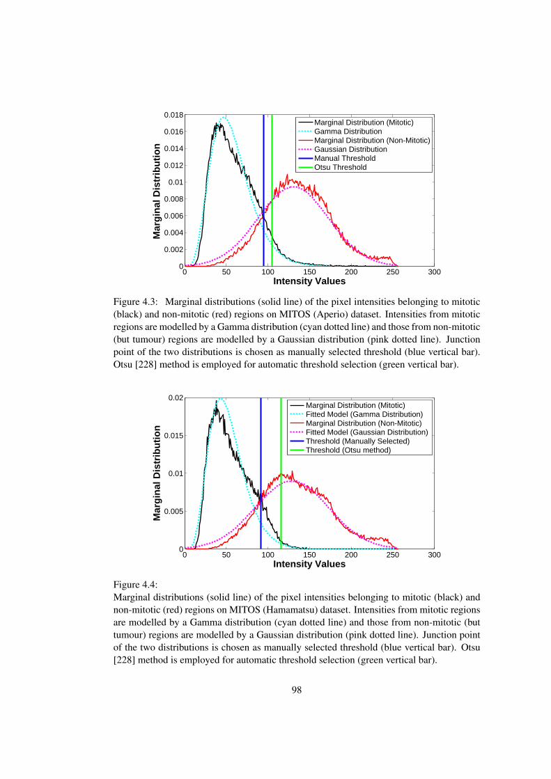
0 50 100 150 200 250 3000

0.002

0.004

0.006

0.008

0.01

0.012

0.014

0.016

0.018

Intensity Values

Mar

gin

al D

istr

ibu

tio

n

Marginal Distribution (Mitotic)Gamma DistributionMarginal Distribution (Non-Mitotic)Gaussian DistributionManual ThresholdOtsu Threshold

Figure 4.3: Marginal distributions (solid line) of the pixel intensities belonging to mitotic(black) and non-mitotic (red) regions on MITOS (Aperio) dataset. Intensities from mitoticregions are modelled by a Gamma distribution (cyan dotted line) and those from non-mitotic(but tumour) regions are modelled by a Gaussian distribution (pink dotted line). Junctionpoint of the two distributions is chosen as manually selected threshold (blue vertical bar).Otsu [228] method is employed for automatic threshold selection (green vertical bar).

0 50 100 150 200 250 3000

0.005

0.01

0.015

0.02

Intensity Values

Mar

gin

al D

istr

ibu

tio

n

Marginal Distribution (Mitotic)Fitted Model (Gamma Distribution)Marginal Distribution (Non-Mitotic)Fitted Model (Gaussian Distribution) Threshold (Manually Selected)Threshold (Otsu method)

Figure 4.4:Marginal distributions (solid line) of the pixel intensities belonging to mitotic (black) andnon-mitotic (red) regions on MITOS (Hamamatsu) dataset. Intensities from mitotic regionsare modelled by a Gamma distribution (cyan dotted line) and those from non-mitotic (buttumour) regions are modelled by a Gaussian distribution (pink dotted line). Junction pointof the two distributions is chosen as manually selected threshold (blue vertical bar). Otsu[228] method is employed for automatic threshold selection (green vertical bar).

98

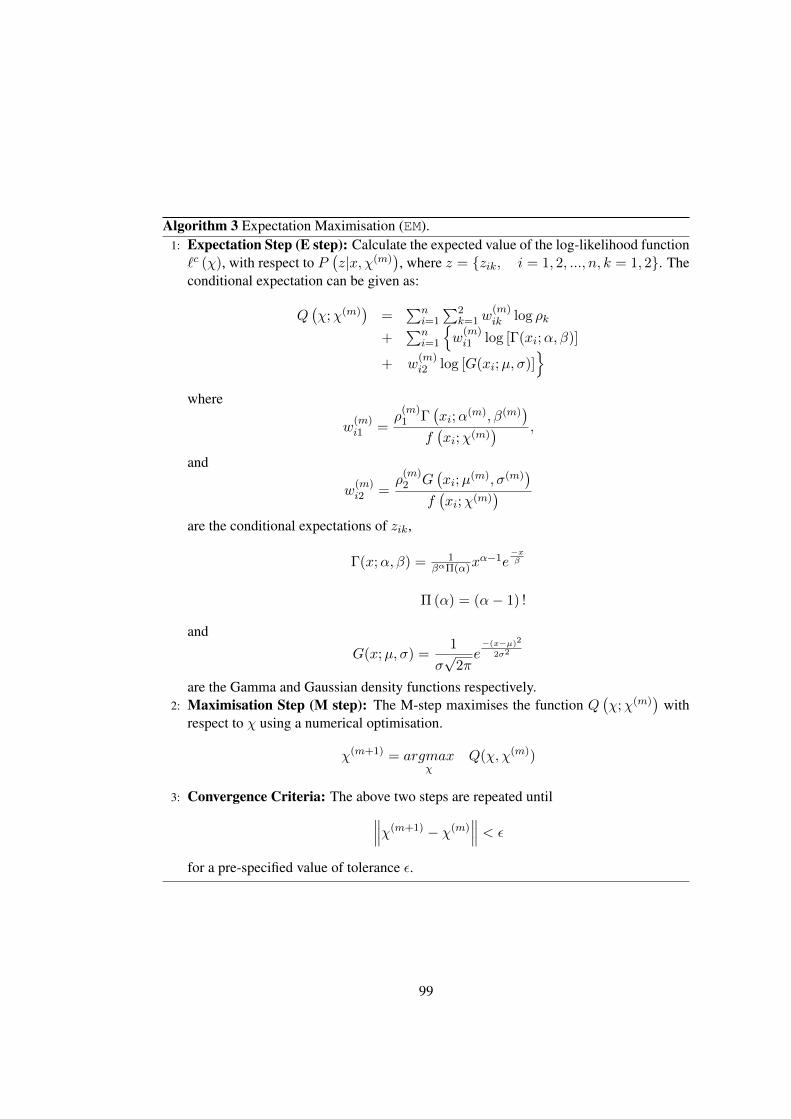
Algorithm 3 Expectation Maximisation (EM).1: Expectation Step (E step): Calculate the expected value of the log-likelihood function`c (χ), with respect to P

(z|x, χ(m)

), where z = {zik, i = 1, 2, ..., n, k = 1, 2}. The

conditional expectation can be given as:

Q(χ;χ(m)

)=

∑ni=1

∑2k=1w

(m)ik log ρk

+∑n

i=1

{w

(m)i1 log [Γ(xi;α, β)]

+ w(m)i2 log [G(xi;µ, σ)]

}

where

w(m)i1 =

ρ(m)1 Γ

(xi;α

(m), β(m))

f(xi;χ(m)

) ,

and

w(m)i2 =

ρ(m)2 G

(xi;µ

(m), σ(m))

f(xi;χ(m)

)

are the conditional expectations of zik,

Γ(x;α, β) = 1βαΠ(α)x

α−1e−xβ

Π (α) = (α− 1) !

and

G(x;µ, σ) =1

σ√

2πe−(x−µ)2

2σ2

are the Gamma and Gaussian density functions respectively.2: Maximisation Step (M step): The M-step maximises the function Q

(χ;χ(m)

)with

respect to χ using a numerical optimisation.

χ(m+1) = argmaxχ

Q(χ, χ(m))

3: Convergence Criteria: The above two steps are repeated until∥∥∥χ(m+1) − χ(m)

∥∥∥ < ε

for a pre-specified value of tolerance ε.

99

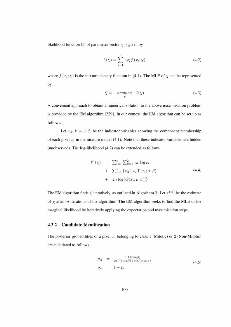
likelihood function (`) of parameter vector χ is given by

` (χ) =n∑

i=1

log f (xi;χ) (4.2)

where f (xi;χ) is the mixture density function in (4.1). The MLE of χ can be represented

by

χ = argmaxχ

`(χ) (4.3)

A convenient approach to obtain a numerical solution to the above maximisation problem

is provided by the EM algorithm [229]. In our context, the EM algorithm can be set up as

follows.

Let zik, k = 1, 2, be the indicator variables showing the component membership

of each pixel xi in the mixture model (4.1). Note that these indicator variables are hidden

(unobserved). The log-likelihood (4.2) can be extended as follows:

`c (χ) =∑n

i=1

∑2k=1 zik log ρk

+∑n

i=1 {zi1 log [Γ(xi;α, β)]

+ zi2 log [G(xi;µ, σ)]}

(4.4)

The EM algorithm finds χ iteratively, as outlined in Algorithm 3. Let χ(m) be the estimate

of χ after m iterations of the algorithm. The EM algorithm seeks to find the MLE of the

marginal likelihood by iteratively applying the expectation and maximisation steps.

4.3.2 Candidate Identification

The posterior probabilities of a pixel xi belonging to class 1 (Mitotic) or 2 (Non-Mitotic)

are calculated as follows,

pi1 = ρ1Γ(x;α,β)ρ1Γ(xi;α,β)+ρ2G(xi;µ,σ)

pi2 = 1− pi1(4.5)

100

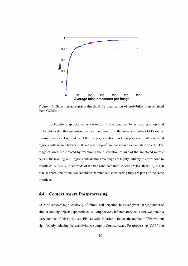
0 50 100 150 200 250 3000

0.2

0.4

0.6

0.8

1

Average false detections per image

Re

ca

ll

Figure 4.5: Selecting appropriate threshold for binarisation of probability map obtainedfrom GGMM.

Probability map obtained as a result of (4.5) is binarised by estimating an optimal

probability value that maximise the recall and minimise the average number of FPs on the

training data (see Figure 4.5). After the segmentation has been performed, all connected

regions with an area between 10µm2 and 100µm2 are considered as candidate objects. The

range of sizes is estimated by examining the distribution of size of the annotated mitotic

cells in the training set. Regions outside this area range are highly unlikely to correspond to

mitotic cells. Lastly, if centroids of the two candidate mitotic cells are less than 4.5µm (20

pixels) apart, one of the two candidates is removed, considering they are parts of the same

mitotic cell.

4.4 Context Aware Postprocessing

GGMM achieves high sensitivity of mitotic cell detection, however given a large number of

similar looking objects (apoptotic cells, lymphocytes, inflammatory cells etc), we obtain a

large number of false positives (FPs) as well. In order to reduce the number of FPs without

significantly reducing the sensitivity, we employ Context Aware Postprocessing (CAPP) on

101

Figure 4.6: Four examples of 50× 50 context patches, cropped around the bounding box ofcandidate mitotic cells (detected using the proposed GGMM algorithm). First 2 (from left)are mitotic, last 2 are false positives.

the results of candidate detection. The motivation for CAPP can be demonstrated through

Figure 4.6, where the context (surrounding texture) of mitotic cells can be seen to be sig-

nificantly different from the context of non-mitotic cells. We use this clue and use a set of

texture features in a classification framework to produce final detections of the mitotic cells.

More specifically, we define a context window of size 81×811around the bounding

box of each potential mitotic cell. In this context window, we compute following texture

features: 32 phase gradient features (16 orientations, 2 scales) [126], 1 roughness feature,

1 entropy feature. From each of these 34 features, 4 representative features were com-

puted: (1) mean, (2) standard deviation, (3) skewness, (4) kurtosis. This generates a 136-

dimensional features vector for each pixel inside the context window. This vector is used to

train an SVM classifier with a Gaussian kernel.

4.5 Cell Words: Cell level Modelling of Mitotic Cells

In this section, we employ a novel appearance based framework for modelling the visual

appearance of cells in histopathology images [38]. Rather than calculating classical fea-

tures (colour, shape, texture), we propose a discriminative dictionary learning (DDL) based

paradigm to model the visual appearance of cells that intrinsically takes into account various

features including colour, shape, texture, and context of cells. The proposed model aims at

learning a dictionary (with class-specific atoms) that simultaneously has both good recon-1See Section 4.6.2 for the intuition behind choosing this window size.

102

struction and high discriminability. Moreover, it exploits some of the attractive properties

of sparse methods (e.g. robustness to noise and compact representation of the data) in order

to learn discriminative representations of complex biological objects. Fisher DDL [230],

the closest work to the proposed model (4.6), employs Fisher discriminant criterion in ad-

dition to the proposed objective function in (4.6), to minimise within-class variation and

maximise between-class variation of sparse codes. However, the Fisher term, which makes

insignificant improvement in the classification accuracy of the model, is computationally

expensive to compute, thus makes the model inefficient for histological images.

Recently, some DDL algorithms have been proposed in the literature. Discrimina-

tive K-SVD [231] uses a linear regression term in a dictionary learning objective function

which penalises non-discriminative atoms. The by-product of the learning process is a

linear classifier that can be directly applied to the learned sparse code. Label consistent

K-SVD [232] adds a label consistent term into the objective function of the discriminative

K-SVD method. The label consistent term encourages the use of atoms with the same la-

bel to reconstruct a data point. Structured incoherent dictionary learning [233] integrates a

term into the objective function that minimises the covariance between atoms of different

classes, so as to circumvent the overlapping of atoms from different classes.

Let c ∈ {C1,C2} denotes a class index, where C1 and C2 represent two different

classes of cells, mitotic cells and non-mitotic cells in our case. Let X = [XC1,XC2] ∈

Rm×N , with Xc = [xc,1, ...,xc,nc ] ∈ Rm×nc be a matrix whose columns are patches from

class c, m be the number of pixels in a patch, N be the total number of training samples,

and nc be the number of training samples of class c. Let D = [DC1,DC2] ∈ Rm×K , with

Dc = [dc,1, ...,dc,kc ] ∈ Rm×kc be the dictionary for class c containing kc atoms, and K be

the total number of atoms. Let A = [AC1,AC2] ∈ RK×N , with Ac = [αc,1, ...,αc,nc ] ∈

RK×nc be the sparse code matrix corresponding to Xc. Our task is to solve the following

103

optimisation problem:

minD,A

∑

c

ν(Xc,D,Ac) + λ‖Ac‖1, subject to dTc,jdc,j = 1 ∀j = 1, ..., kc, (4.6)

where

ν(Xc,D,Ac) = ‖Xc −DAc‖2F+‖Xc −DcA(c)c ‖2F+γ

∑

l 6=c‖DlA

(l)c ‖2F (4.7)

and ‖·‖1,‖·‖F denote the l1 norm, and the Frobenius norm of a matrix, respectively, A(l)c

denotes a sub-matrix of Ac that corresponds to Dl, and λ is the sparsity regularisation

parameter. In (4.7), the first term refers to the reconstruction error of Xc using the whole

dictionary, the second term refers to the use of Dc for reconstructing Xc, while the last term

refers to the prevention of reconstructing Xc using dictionary atoms from other classes,

penalised by a parameter γ.

The proposed framework can be divided into two phases: (1) learning a data driven

dictionary; (2) classification. During the dictionary learning phase, a dictionary is learned

from the training data by solving the optimisation problem in (4.6). During the classifica-

tion, a test sample is first encoded over the learned dictionary (i.e. represented as a linear

combination of few atoms from the learned dictionary), and then the reconstruction resid-

ual based on the sparse code is used to determine the class of the test sample. Following

subsections briefly outline the two phases of the proposed framework. For details of the

algorithm, the reader is referred to [38].

Learning the Cell Words

In order to learn a data-driven class specific dictionary, following 4 step procedure is

adopted. Note that step 3 and 4 are repeated until stopping criterion such as the number

of iterations or tolerance on the cost of the objective function in (4.6) is met.

1. Dictionary Initialisation: For each class c, perform PCA on Xc where patches are

104

treated as variables and pixels are treated as observations. Use the first kc−1 principal

components and the mean of all patches in Xc to initialise the dictionary D0c .

2. Sparse Code Initialisation: For each class c, initialise sparse code A0c by solving

A0c = arg min

A‖Xc −DcA‖2F ,

subject to ‖αi‖≤ L ∀i = 1, ..., nc (4.8)

in which A = [α1, ..., αnc ] and L is the number of non-zeros elements in αi, via

orthogonal matching pursuit method [234].

3. Dictionary Optimisation: For each class c, find unused atoms in Dtc and replace

them with randomly selected patches from the same class. Find Dt+1c that optimises

(4.9) using block coordinate descent method described in Algorithm 1 in [38].

minDc

‖Xc −DAc‖2F+‖Xc −DcA(c)c ‖2F+γ

∑

l 6=c‖DcA

(c)l ‖2F

subject to dTc,jdc,j = 1 ∀j = 1, ..., kc (4.9)

4. Sparse Code Optimisation: For each class c, find At+1c that optimises (4.10), also

known as lasso [235], using Algorithm 2 in [38].

minAc

ν(Xc,D,Ac) + λ‖Ac‖1 (4.10)

Classification

We calculate a sparse code α∗ of x using the whole learned dictionary D,

α∗ = arg minα∈Rm

{‖x−Dα‖22+τ‖α‖1

}(4.11)

105

where τ is a sparsity regularisation parameter. Then, we assign a class label for x based on

the minimum reconstruction error of class-specific dictionaries,

c∗ = arg minc∈{C1,C2}

‖x−Dcα∗‖2 (4.12)

4.6 Parameters, Experimental Setup & Evaluation

We evaluate our algorithm on two datasets: WarMiCe and MITOS datasets. The details

about the datasets are provided in Section 1.6. This section provides details about the

experimental settings of candidate detection and classification algorithms proposed in this

chapter.

4.6.1 Candidate Detection

GGMM model is learned from a small set of training images randomly selected from the

MITOS (Aperio) dataset. Since all the images were stain normalised, therefore model

trained on the MITOS (Aperio) dataset was used without any change on the MITOS (Hama-

matsu) and WarMiCe datasets. Algorithm 3 was run for 500 iterations with tolerance (ε)

set to 0.01. The choice of these parameters was based on some preliminary experiments.

We did not observe significant improvement in performance of the algorithm by further in-

creasing the number of iterations or further reducing ε. Although EM provides estimates

for ρ1 and ρ2 in (4.1), more accurate estimates (ρ1 = 0.0014 and ρ2 = 0.9986) were used

based on the ratio of mitotic and non-mitotic data used for model fitting.

4.6.2 Candidate Classification

As majority of mitotic cells in the two datasets fall in the range of 30×30 to 60×60 pixels,

therefore in order to incorporate the surrounding context along with the candidate mitotic

cells, we choose a patch size of 81×81 (i.e. 10 pixels margin on each side of the image) as a

trade-off between the amount of context and the computational burden. However, since we

106

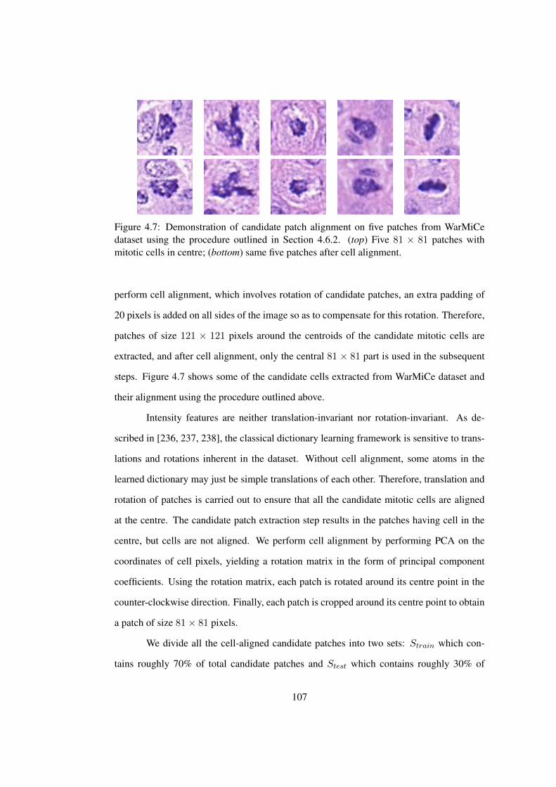
Figure 4.7: Demonstration of candidate patch alignment on five patches from WarMiCedataset using the procedure outlined in Section 4.6.2. (top) Five 81 × 81 patches withmitotic cells in centre; (bottom) same five patches after cell alignment.

perform cell alignment, which involves rotation of candidate patches, an extra padding of

20 pixels is added on all sides of the image so as to compensate for this rotation. Therefore,

patches of size 121 × 121 pixels around the centroids of the candidate mitotic cells are

extracted, and after cell alignment, only the central 81 × 81 part is used in the subsequent

steps. Figure 4.7 shows some of the candidate cells extracted from WarMiCe dataset and

their alignment using the procedure outlined above.

Intensity features are neither translation-invariant nor rotation-invariant. As de-

scribed in [236, 237, 238], the classical dictionary learning framework is sensitive to trans-

lations and rotations inherent in the dataset. Without cell alignment, some atoms in the

learned dictionary may just be simple translations of each other. Therefore, translation and

rotation of patches is carried out to ensure that all the candidate mitotic cells are aligned

at the centre. The candidate patch extraction step results in the patches having cell in the

centre, but cells are not aligned. We perform cell alignment by performing PCA on the

coordinates of cell pixels, yielding a rotation matrix in the form of principal component

coefficients. Using the rotation matrix, each patch is rotated around its centre point in the

counter-clockwise direction. Finally, each patch is cropped around its centre point to obtain

a patch of size 81× 81 pixels.

We divide all the cell-aligned candidate patches into two sets: Strain which con-

tains roughly 70% of total candidate patches and Stest which contains roughly 30% of

107

total candidate patches. We further split candidate patches in Strain into Xtrain (70%) and

Xvalidate (30%), respectively. Xtrain is used in the training procedure of the proposed DDL

method, while Xvalidate is used to monitor the classification performance at each iteration

and to avoid over-fitting. We select the dictionary from the iteration that gives the highest

classification performance on Xvalidate and perform classification of patches from Stest.

In order to reduce the effect from random partition of Strain into Xtrain and Xtest,

we run each experiment for 10 repetitions. For each repetition i, we generate the set of

detections for Stest and count the number Ntp,i of TP (i.e. detections whose centroids

are closer than 8µm from the GT centroid), FP (Nfp,i) and FN (Nfn,i). The total num-

bers of TP, FN, and FP are given by (Ntp =∑10

i=1Ntp,i), (Nfn =∑10

i=1Nfn,i), and

(Nfp =∑10

i=1Nfp,i), respectively. The following performance measures are calculated:

recall (Re = Ntp/(Ntp + Nfn)), precision (Pr = Ntp/(Ntp + Nfp)) and F1-score (F1 =

2Pr×Re/(Pr+Re)).

For CAPP, we use the LIBSVM implementation [239]. We use grid search to find

optimal parameters for the soft margin and Gaussian kernel parameters of SVM. Moreover

for SVM, a higher penalty for misclassification of mitotic class was used, since the data

obtained as a result of candidate identification step (Section 4.3) was highly imbalanced

(mitotic-20.1%, non-mitotic-79.9%).

For cell words, we use blue ratio (BR), that measures the spatial distribution of nu-

clear content of an image, as input to the proposed DDL framework [209]. Using colour

channels (R,G,B) would add a non-trivial computational burden on the dictionary learn-

ing algorithms, therefore BR was used as it incorporates information from all three colour

channels.

BR = 100

(B

1 +R+G

)(256

1 +R+G+B

). (4.13)

where R, G and B refer to the red, green and blue channels of a coloured RGB image.

To make the input data consistent with the dictionary optimisation procedure that does not

constrain coefficients of atoms to be non-negative, all the data are linearly transformed to

108

have zero median. A stopping criterion for the algorithm is that the relative difference

on the cost of the objective function for the consecutive iterations is less than 10−6. We

manually select regularisation parameters λ for training, and τ for classification such that a

certain level of average sparseness (0.8) is attained when the algorithm converges. Similarly,

number of atoms were fixed to [40, 40], i.e. 40 atoms for mitotic class and 40 atoms for non-

mitotic class. The choice of parameters was empirically found to produce highly accurate

results. For details on various experiments related to the choice of these parameters, refer

to [38].

4.7 Results and Discussion

4.7.1 Candidate Detection

Figure 4.8 demonstrates the superiority of the proposed GGMM algorithm compared to

manually selected threshold2 and Otsu threshold [228]. It can be observed that GGMM

produces high sensitivity and significantly high PPV as compared to manual thresholding

and Otsu thresholding. Even though manual and Otsu thresholding produce marginally

higher sensitivity, the PPV for both of these methods is relatively very low. A similar

trend of detection performance was observed on the MITOS (Hamamatsu) and WarMiCe

datasets.

4.7.2 CAPP vs. Cell Words on the MITOS dataset

Here we compare the performance of CAPP - our baseline mitotic cells classification sys-

tem with cell words on MITOS dataset. Incremental improvement in performance of the

proposed system can be observed from the results presented in Table 4.2, where we demon-

strate that if we do not apply any postprocessing, a low F1-score is achieved as large number

of false positives, which look like mitotic cells, are detected (see Figure 4.9). Using CAPP

on top provides an improvement of 3.12× and 3.93× in terms of F1-score on Aperio and2See Figure 4.3 and Figure 4.4 for how this threshold is selected.

109

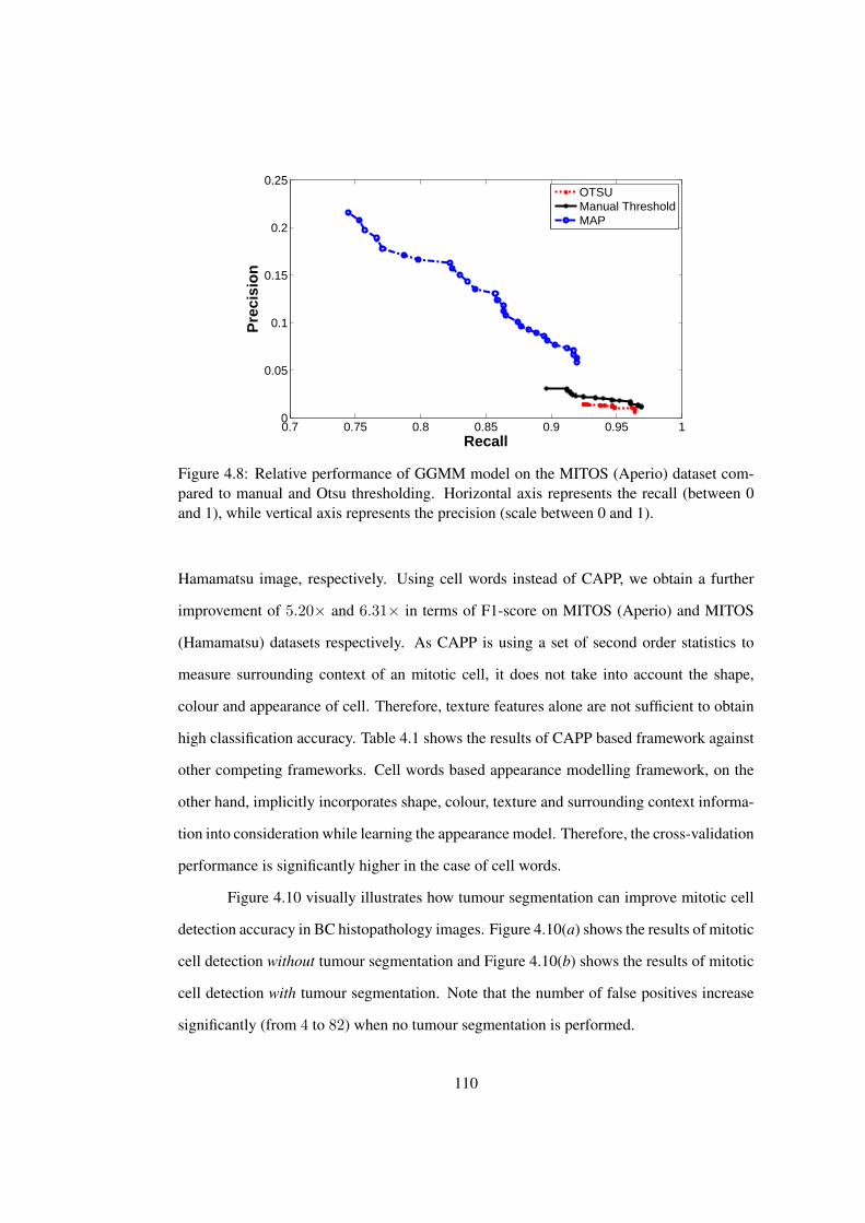
0.7 0.75 0.8 0.85 0.9 0.95 10

0.05

0.1

0.15

0.2

0.25

Pre

cisi

on

Recall

OTSUManual ThresholdMAP

Figure 4.8: Relative performance of GGMM model on the MITOS (Aperio) dataset com-pared to manual and Otsu thresholding. Horizontal axis represents the recall (between 0and 1), while vertical axis represents the precision (scale between 0 and 1).

Hamamatsu image, respectively. Using cell words instead of CAPP, we obtain a further

improvement of 5.20× and 6.31× in terms of F1-score on MITOS (Aperio) and MITOS

(Hamamatsu) datasets respectively. As CAPP is using a set of second order statistics to

measure surrounding context of an mitotic cell, it does not take into account the shape,

colour and appearance of cell. Therefore, texture features alone are not sufficient to obtain

high classification accuracy. Table 4.1 shows the results of CAPP based framework against

other competing frameworks. Cell words based appearance modelling framework, on the

other hand, implicitly incorporates shape, colour, texture and surrounding context informa-

tion into consideration while learning the appearance model. Therefore, the cross-validation

performance is significantly higher in the case of cell words.

Figure 4.10 visually illustrates how tumour segmentation can improve mitotic cell

detection accuracy in BC histopathology images. Figure 4.10(a) shows the results of mitotic

cell detection without tumour segmentation and Figure 4.10(b) shows the results of mitotic

cell detection with tumour segmentation. Note that the number of false positives increase

significantly (from 4 to 82) when no tumour segmentation is performed.

110

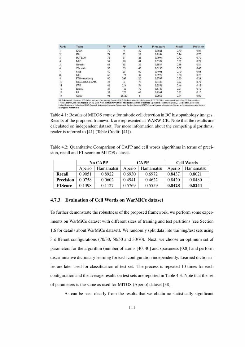
Table 4.1: Results of MITOS contest for mitotic cell detection in BC histopathology images.Results of the proposed framework are represented as WARWICK. Note that the results arecalculated on independent dataset. For more information about the competing algorithms,reader is referred to [41] (Table Credit: [41]).

Table 4.2: Quantitative Comparison of CAPP and cell words algorithms in terms of preci-sion, recall and F1-score on MITOS dataset.

No CAPP CAPP Cell WordsAperio Hamamatsu Aperio Hamamatsu Aperio Hamamatsu

Recall 0.9051 0.8922 0.6930 0.6972 0.8437 0.8021Precision 0.0758 0.0602 0.4941 0.4622 0.8420 0.8480F1Score 0.1398 0.1127 0.5769 0.5559 0.8428 0.8244

4.7.3 Evaluation of Cell Words on WarMiCe dataset

To further demonstrate the robustness of the proposed framework, we perform some exper-

iments on WarMiCe dataset with different sizes of training and test partitions (see Section

1.6 for details about WarMiCe dataset). We randomly split data into training/test sets using

3 different configurations (70/30, 50/50 and 30/70). Next, we choose an optimum set of

parameters for the algorithm (number of atoms [40, 40] and sparseness [0.8]) and perform

discriminative dictionary learning for each configuration independently. Learned dictionar-

ies are later used for classification of test set. The process is repeated 10 times for each

configuration and the average results on test sets are reported in Table 4.3. Note that the set

of parameters is the same as used for MITOS (Aperio) dataset [38].

As can be seen clearly from the results that we obtain no statistically significant

111

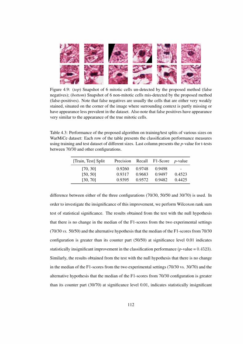
Figure 4.9: (top) Snapshot of 6 mitotic cells un-detected by the proposed method (falsenegatives); (bottom) Snapshot of 6 non-mitotic cells mis-detected by the proposed method(false-positives). Note that false negatives are usually the cells that are either very weaklystained, situated on the corner of the image where surrounding context is partly missing orhave appearance less prevalent in the dataset. Also note that false positives have appearancevery similar to the appearance of the true mitotic cells.

Table 4.3: Performance of the proposed algorithm on training/test splits of various sizes onWarMiCe dataset: Each row of the table presents the classification performance measuresusing training and test dataset of different sizes. Last column presents the p-value for t-testsbetween 70/30 and other configurations.

[Train, Test] Split Precision Recall F1-Score p-value

[70, 30] 0.9260 0.9748 0.9498 -[50, 50] 0.9317 0.9683 0.9497 0.4523[30, 70] 0.9395 0.9572 0.9482 0.4425

difference between either of the three configurations (70/30, 50/50 and 30/70) is used. In

order to investigate the insignificance of this improvement, we perform Wilcoxon rank sum

test of statistical significance. The results obtained from the test with the null hypothesis

that there is no change in the median of the F1-scores from the two experimental settings

(70/30 vs. 50/50) and the alternative hypothesis that the median of the F1-scores from 70/30

configuration is greater than its counter part (50/50) at significance level 0.01 indicates

statistically insignificant improvement in the classification performance (p-value = 0.4523).

Similarly, the results obtained from the test with the null hypothesis that there is no change

in the median of the F1-scores from the two experimental settings (70/30 vs. 30/70) and the

alternative hypothesis that the median of the F1-scores from 70/30 configuration is greater

than its counter part (30/70) at significance level 0.01, indicates statistically insignificant

112

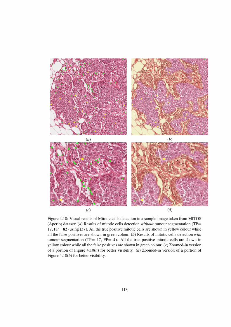
(a) (b)

(c) (d)

Figure 4.10: Visual results of Mitotic cells detection in a sample image taken from MITOS(Aperio) dataset: (a) Results of mitotic cells detection without tumour segmentation (TP=17, FP= 82) using [37]. All the true positive mitotic cells are shown in yellow colour whileall the false positives are shown in green colour. (b) Results of mitotic cells detection withtumour segmentation (TP= 17, FP= 4). All the true positive mitotic cells are shown inyellow colour while all the false positives are shown in green colour. (c) Zoomed-in versionof a portion of Figure 4.10(a) for better visibility. (d) Zoomed-in version of a portion ofFigure 4.10(b) for better visibility.

113

improvement in the classification performance (p-value = 0.4425).

The trend shown in Table 4.3 is somewhat different from what we noticed in sec-

tion 4.5.3 [38], where we noticed that as we increase the proportion of training data, the

performance of the proposed algorithm showed statistically significant improvement. This

can be attributed to the difference in number of mitotic cells in the two datasets. MITOS

has 326 mitotic cells in total, whereas WarMiCe has 1324 mitotic cells. In 30/70 config-

uration, MITOS uses just 97 mitotic cells, as compared to 397 in WarMiCe, to model the

visual appearance of mitotic cells. This is a significant difference (≈ 309% more training

data). Dictionary learned based on WarMiCe dataset captures variation in visual appearance

of mitotic cells and provides a richer representation of mitotic cells that results in higher

out-of-sample accuracy even with 30/70 configuration.

4.7.4 Computational Efficiency

In this section, we present a comparison of computational efficiency of the GGMM, CAPP

and cell words candidate detection and classification frameworks proposed in this chapter.

Table 4.4 presents a comparison of running times of various components of the proposed

mitotic cell detection framework. Overall dictionary learning phase is the most computa-

tionally demanding part of the framework. However, once the dictionary is learned from

the data, classification is relatively efficient. For GGMM, training time is the time required

to estimate the parameters of GGMM. Evaluation time is the time required to calculate the

likelihood estimates for Gamma and Gaussian distribution in (4.5) on a test image of size

512 × 512 pixels. For CAPP, we explicitly report the time to perform grid search on the

parameter space of SVM with Gaussian kernel. We also report the time required to train the

classifier on optimal set of parameters and the time required to test a single candidate cell

using the trained model. All results are generated on 12-core Mac Pro with 64GB RAM

using 64-bit MATLAB R© 2014a.

114

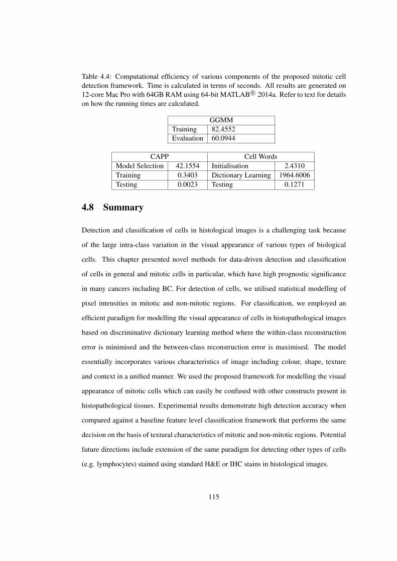
Table 4.4: Computational efficiency of various components of the proposed mitotic celldetection framework. Time is calculated in terms of seconds. All results are generated on12-core Mac Pro with 64GB RAM using 64-bit MATLAB R© 2014a. Refer to text for detailson how the running times are calculated.

GGMMTraining 82.4552Evaluation 60.0944

CAPP Cell WordsModel Selection 42.1554 Initialisation 2.4310Training 0.3403 Dictionary Learning 1964.6006Testing 0.0023 Testing 0.1271

4.8 Summary

Detection and classification of cells in histological images is a challenging task because

of the large intra-class variation in the visual appearance of various types of biological

cells. This chapter presented novel methods for data-driven detection and classification

of cells in general and mitotic cells in particular, which have high prognostic significance

in many cancers including BC. For detection of cells, we utilised statistical modelling of

pixel intensities in mitotic and non-mitotic regions. For classification, we employed an

efficient paradigm for modelling the visual appearance of cells in histopathological images

based on discriminative dictionary learning method where the within-class reconstruction

error is minimised and the between-class reconstruction error is maximised. The model

essentially incorporates various characteristics of image including colour, shape, texture

and context in a unified manner. We used the proposed framework for modelling the visual

appearance of mitotic cells which can easily be confused with other constructs present in

histopathological tissues. Experimental results demonstrate high detection accuracy when

compared against a baseline feature level classification framework that performs the same

decision on the basis of textural characteristics of mitotic and non-mitotic regions. Potential

future directions include extension of the same paradigm for detecting other types of cells

(e.g. lymphocytes) stained using standard H&E or IHC stains in histological images.

115

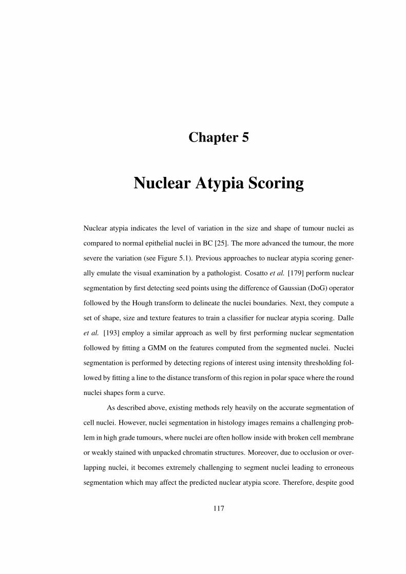
Chapter 5

Nuclear Atypia Scoring

Nuclear atypia indicates the level of variation in the size and shape of tumour nuclei as

compared to normal epithelial nuclei in BC [25]. The more advanced the tumour, the more

severe the variation (see Figure 5.1). Previous approaches to nuclear atypia scoring gener-

ally emulate the visual examination by a pathologist. Cosatto et al. [179] perform nuclear

segmentation by first detecting seed points using the difference of Gaussian (DoG) operator

followed by the Hough transform to delineate the nuclei boundaries. Next, they compute a

set of shape, size and texture features to train a classifier for nuclear atypia scoring. Dalle

et al. [193] employ a similar approach as well by first performing nuclear segmentation

followed by fitting a GMM on the features computed from the segmented nuclei. Nuclei

segmentation is performed by detecting regions of interest using intensity thresholding fol-

lowed by fitting a line to the distance transform of this region in polar space where the round

nuclei shapes form a curve.

As described above, existing methods rely heavily on the accurate segmentation of

cell nuclei. However, nuclei segmentation in histology images remains a challenging prob-

lem in high grade tumours, where nuclei are often hollow inside with broken cell membrane

or weakly stained with unpacked chromatin structures. Moreover, due to occlusion or over-

lapping nuclei, it becomes extremely challenging to segment nuclei leading to erroneous

segmentation which may affect the predicted nuclear atypia score. Therefore, despite good

117

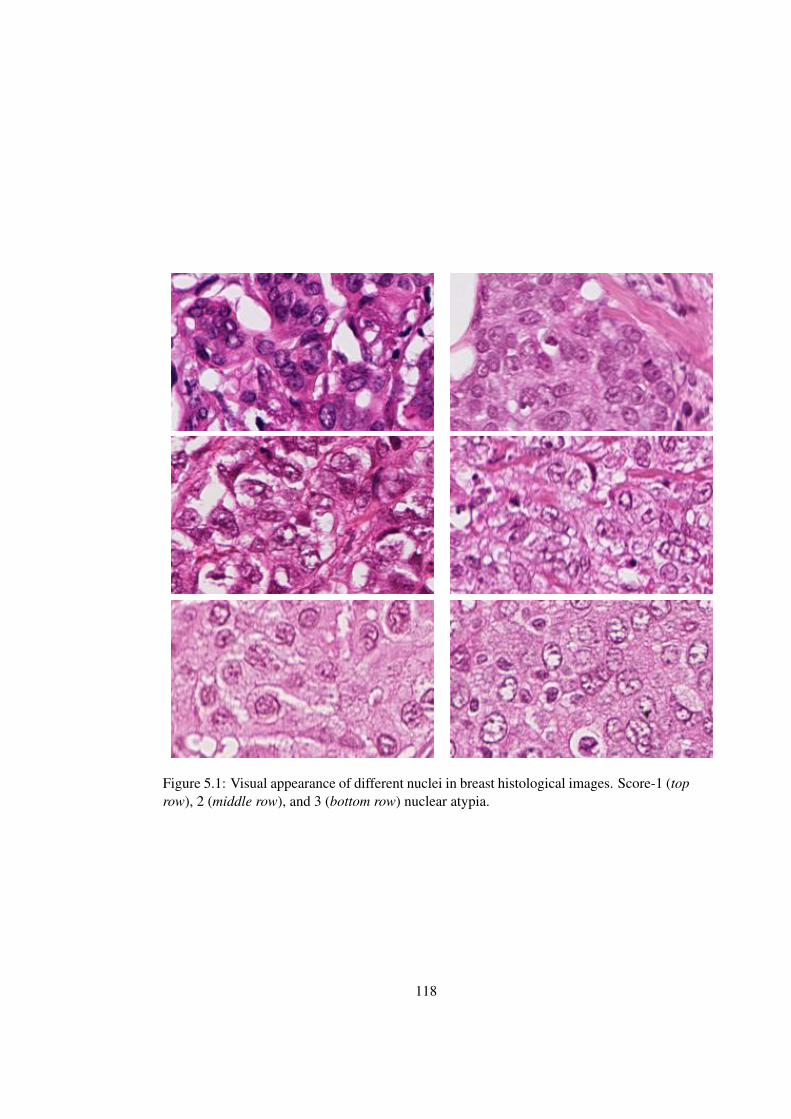
Figure 5.1: Visual appearance of different nuclei in breast histological images. Score-1 (toprow), 2 (middle row), and 3 (bottom row) nuclear atypia.

118

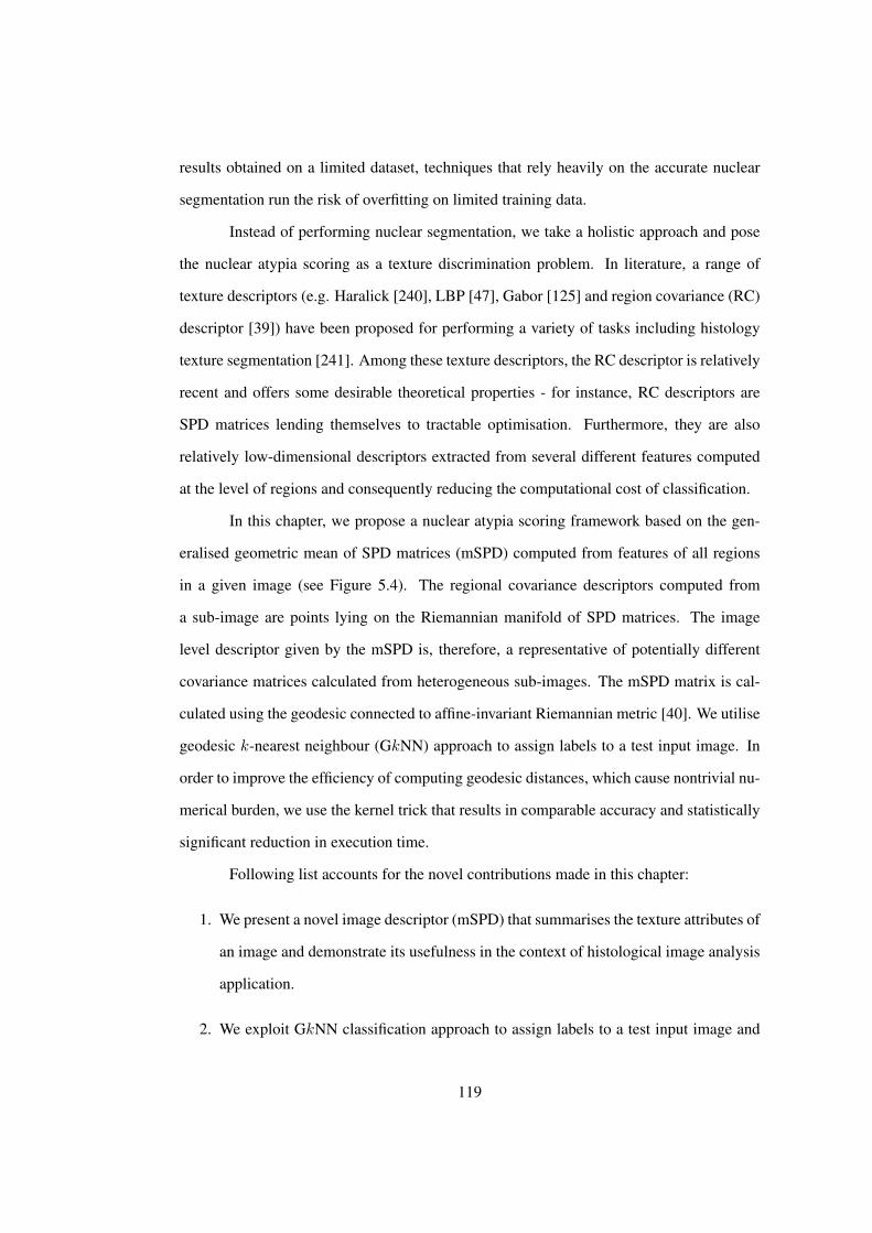
results obtained on a limited dataset, techniques that rely heavily on the accurate nuclear

segmentation run the risk of overfitting on limited training data.

Instead of performing nuclear segmentation, we take a holistic approach and pose

the nuclear atypia scoring as a texture discrimination problem. In literature, a range of

texture descriptors (e.g. Haralick [240], LBP [47], Gabor [125] and region covariance (RC)

descriptor [39]) have been proposed for performing a variety of tasks including histology

texture segmentation [241]. Among these texture descriptors, the RC descriptor is relatively

recent and offers some desirable theoretical properties - for instance, RC descriptors are

SPD matrices lending themselves to tractable optimisation. Furthermore, they are also

relatively low-dimensional descriptors extracted from several different features computed

at the level of regions and consequently reducing the computational cost of classification.

In this chapter, we propose a nuclear atypia scoring framework based on the gen-

eralised geometric mean of SPD matrices (mSPD) computed from features of all regions

in a given image (see Figure 5.4). The regional covariance descriptors computed from

a sub-image are points lying on the Riemannian manifold of SPD matrices. The image

level descriptor given by the mSPD is, therefore, a representative of potentially different

covariance matrices calculated from heterogeneous sub-images. The mSPD matrix is cal-

culated using the geodesic connected to affine-invariant Riemannian metric [40]. We utilise

geodesic k-nearest neighbour (GkNN) approach to assign labels to a test input image. In

order to improve the efficiency of computing geodesic distances, which cause nontrivial nu-

merical burden, we use the kernel trick that results in comparable accuracy and statistically

significant reduction in execution time.

Following list accounts for the novel contributions made in this chapter:

1. We present a novel image descriptor (mSPD) that summarises the texture attributes of

an image and demonstrate its usefulness in the context of histological image analysis

application.

2. We exploit GkNN classification approach to assign labels to a test input image and

119

demonstrate its superiority as compared to the standard classification approaches as

it exploits the structure of Riemannian manifold.

3. We present a comparison with a baseline texture based image classification frame-

work that computes a library of texture features and employs three classification

paradigms to perform nuclear atypia scoring.

4. We present a range of experiments that evaluate the performance of the proposed

nuclear atypia scoring algorithm in terms of classification accuracy as well as com-

putational time. We also evaluate performance of the proposed algorithms, when

certain preprocessing steps like stain normalisation (Chapter 2) and tumour segmen-

tation (Chapter 3) are incorporated in nuclear atypia scoring framework.

The rest of this chapter is organised as follows: Section 5.1 presents a baseline

nuclear atypia scoring framework that is inspired from the standard texture based image

classification approaches which are generally employed in computer vision applications and

histological image analysis applications; Section 5.2 presents the proposed nuclear atypia

scoring framework that utilises mSPD and GkNN to achieve superior performance; Section

5.3 presents a range of experiments conducted to evaluate and compare the performance of

two frameworks and Section 5.4 presents a summary of this chapter.

5.1 Baseline Framework for Nuclear Atypia Scoring

To evaluation the performance of our proposed method, we implement a traditional tex-

ture based image classification framework, that calculates a set of texture features, perform

feature selection in order to remove the redundant and non-discriminative features, and per-

form classification using a machine learning framework. The reason behind choosing this

baseline is three-folded: (1) Our approach to nuclear atypia scoring is quite similar to the

baseline nuclear atypia scoring framework in that it is also holistic in nature as we compute

a texture descriptor and use it in the classification framework; (2) the source codes of exist-

ing algorithms for nuclear atypia scoring in literature are not available; (3) the approach we

120

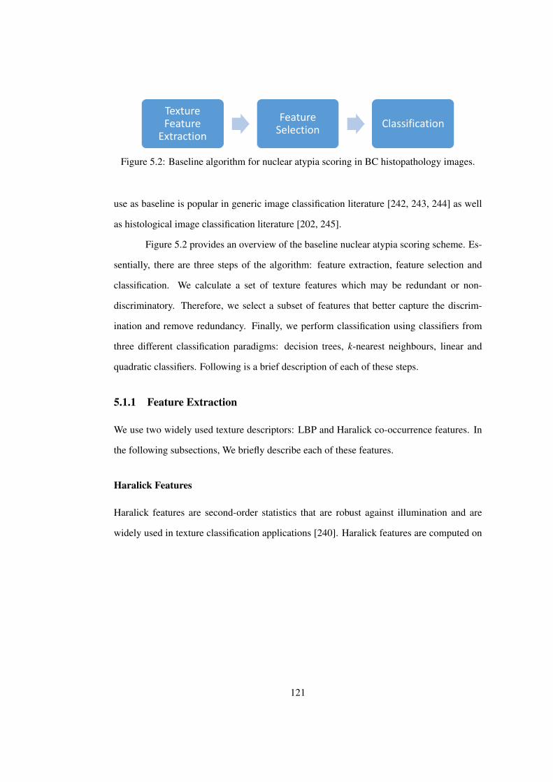
Texture Feature

Extraction

Feature Selection

Classification

Figure 5.2: Baseline algorithm for nuclear atypia scoring in BC histopathology images.

use as baseline is popular in generic image classification literature [242, 243, 244] as well

as histological image classification literature [202, 245].

Figure 5.2 provides an overview of the baseline nuclear atypia scoring scheme. Es-

sentially, there are three steps of the algorithm: feature extraction, feature selection and

classification. We calculate a set of texture features which may be redundant or non-

discriminatory. Therefore, we select a subset of features that better capture the discrim-

ination and remove redundancy. Finally, we perform classification using classifiers from

three different classification paradigms: decision trees, k-nearest neighbours, linear and

quadratic classifiers. Following is a brief description of each of these steps.

5.1.1 Feature Extraction

We use two widely used texture descriptors: LBP and Haralick co-occurrence features. In

the following subsections, We briefly describe each of these features.

Haralick Features

Haralick features are second-order statistics that are robust against illumination and are

widely used in texture classification applications [240]. Haralick features are computed on

121

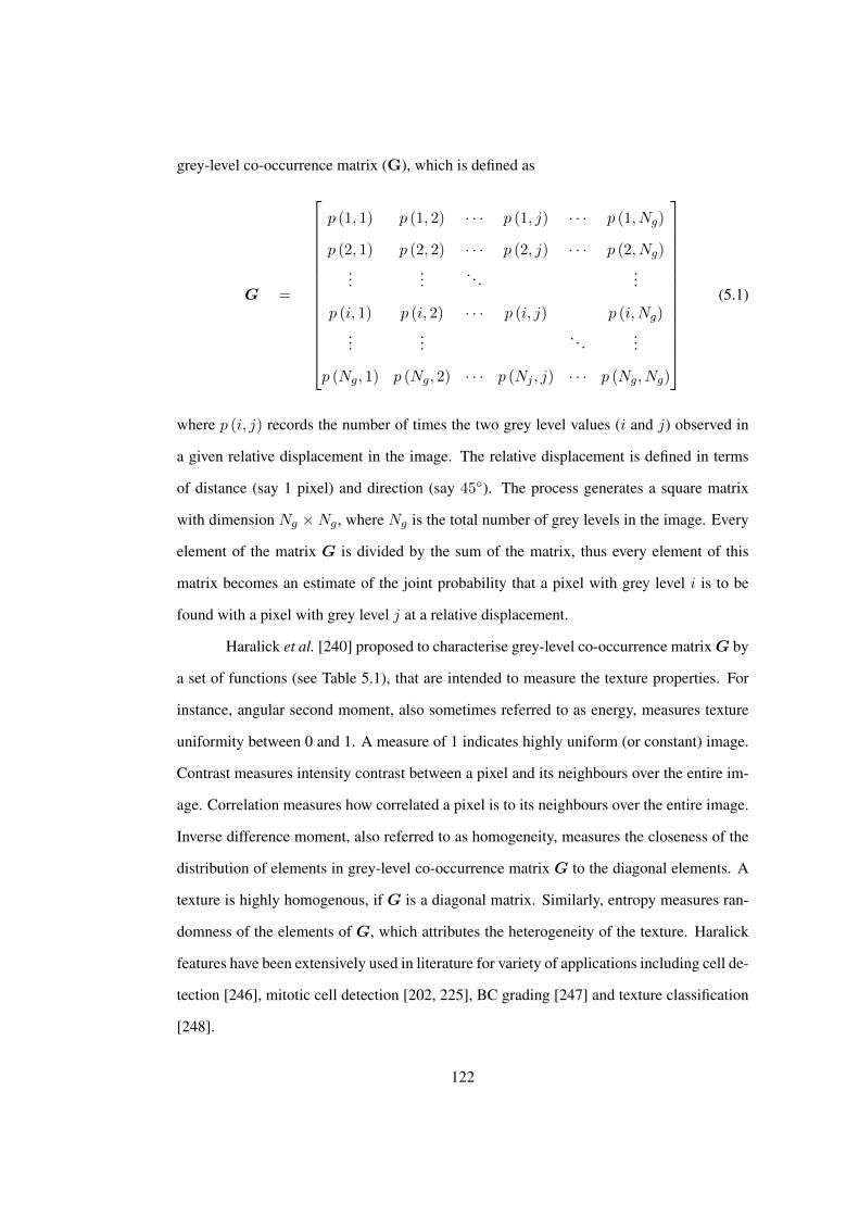
grey-level co-occurrence matrix (G), which is defined as

G =

p (1, 1) p (1, 2) · · · p (1, j) · · · p (1, Ng)

p (2, 1) p (2, 2) · · · p (2, j) · · · p (2, Ng)

......

. . ....

p (i, 1) p (i, 2) · · · p (i, j) p (i,Ng)

......

. . ....

p (Ng, 1) p (Ng, 2) · · · p (Nj , j) · · · p (Ng, Ng)

(5.1)

where p (i, j) records the number of times the two grey level values (i and j) observed in

a given relative displacement in the image. The relative displacement is defined in terms

of distance (say 1 pixel) and direction (say 45◦). The process generates a square matrix

with dimension Ng ×Ng, where Ng is the total number of grey levels in the image. Every

element of the matrix G is divided by the sum of the matrix, thus every element of this

matrix becomes an estimate of the joint probability that a pixel with grey level i is to be

found with a pixel with grey level j at a relative displacement.

Haralick et al. [240] proposed to characterise grey-level co-occurrence matrixG by

a set of functions (see Table 5.1), that are intended to measure the texture properties. For

instance, angular second moment, also sometimes referred to as energy, measures texture

uniformity between 0 and 1. A measure of 1 indicates highly uniform (or constant) image.

Contrast measures intensity contrast between a pixel and its neighbours over the entire im-

age. Correlation measures how correlated a pixel is to its neighbours over the entire image.

Inverse difference moment, also referred to as homogeneity, measures the closeness of the

distribution of elements in grey-level co-occurrence matrix G to the diagonal elements. A

texture is highly homogenous, if G is a diagonal matrix. Similarly, entropy measures ran-

domness of the elements of G, which attributes the heterogeneity of the texture. Haralick

features have been extensively used in literature for variety of applications including cell de-

tection [246], mitotic cell detection [202, 225], BC grading [247] and texture classification

[248].

122

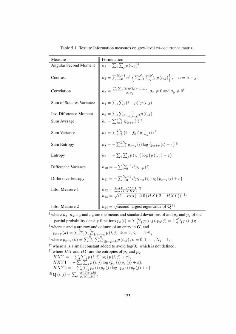
Table 5.1: Texture Information measures on grey-level co-occurrence matrix.

Measure FormulationAngular Second Moment h1 =

∑i

∑j p (i, j)2

Contrast h2 =∑Ng−1

n=0 n2{∑Ng

i=1

∑Ngj=1 p (i, j)

}, n = |i− j|

Correlation h3 =∑i

∑j (ij)p(i,j)−µxµy

σxσy, σx 6= 0 and σy 6= 0†

Sum of Squares Variance h4 =∑

i

∑j (i− µ)2p (i, j)

Inv. Difference Moment h5 =∑

i

∑j

11+(i−j)2 p (i, j)

Sum Average h6 =∑2Ng

i=2 ipx+y (i) ‡

Sum Variance h7 =∑2Ng

i=2 (i− f8)2px+y (i) §

Sum Entropy h8 = −∑2Ngi=2 px+y (i) log {px+y (i) + ε} ††

Entropy h9 = −∑i

∑j p (i, j) log {p (i, j) + ε}

Difference Variance h10 = −∑Ng−1i=0 i2px−y (i)

Difference Entropy h11 = −∑Ng−1i=0 i2px−y (i) log {px−y (i) + ε}

Info. Measure 1 h12 = HXY−HXY 1max {HX,HY }

‡‡

h13 =√

(1− exp (−2.0 (HXY 2−HXY ))) ‡‡

Info. Measure 2 h14 =√

second largest eigenvalue of Q §§

†where µx, µy, σx and σy are the means and standard deviations of and px and py of thepartial probability density functions px(i) =

∑Ngj=1 p (i, j), py(j) =

∑Ngi=1 p (i, j);

‡where x and y are row and column of an entry inG, andpx+y (k) =

∑Ngi=1

∑Ngj=1i+j=k p (i, j) , k = 2, 3, · · · , 2Ng;

§where px−y (k) =∑Ng

i=1

∑Ngj=1|i−j|=k p (i, j) , k = 0, 1, · · · , Ng − 1;

††where ε is a small constant added to avoid log(0), which is not defined;‡‡where HX and HY are the entropies of px and py,HXY = −∑i

∑j p (i, j) log {p (i, j) + ε},

HXY 1 = −∑i

∑j p (i, j) log {px (i) py (j) + ε},

HXY 2 = −∑i

∑j px (i) py (j) log {px (i) py (j) + ε};

§§Q (i, j) =∑

kp(i,k)p(j,k)px(i)py(k) ;

123

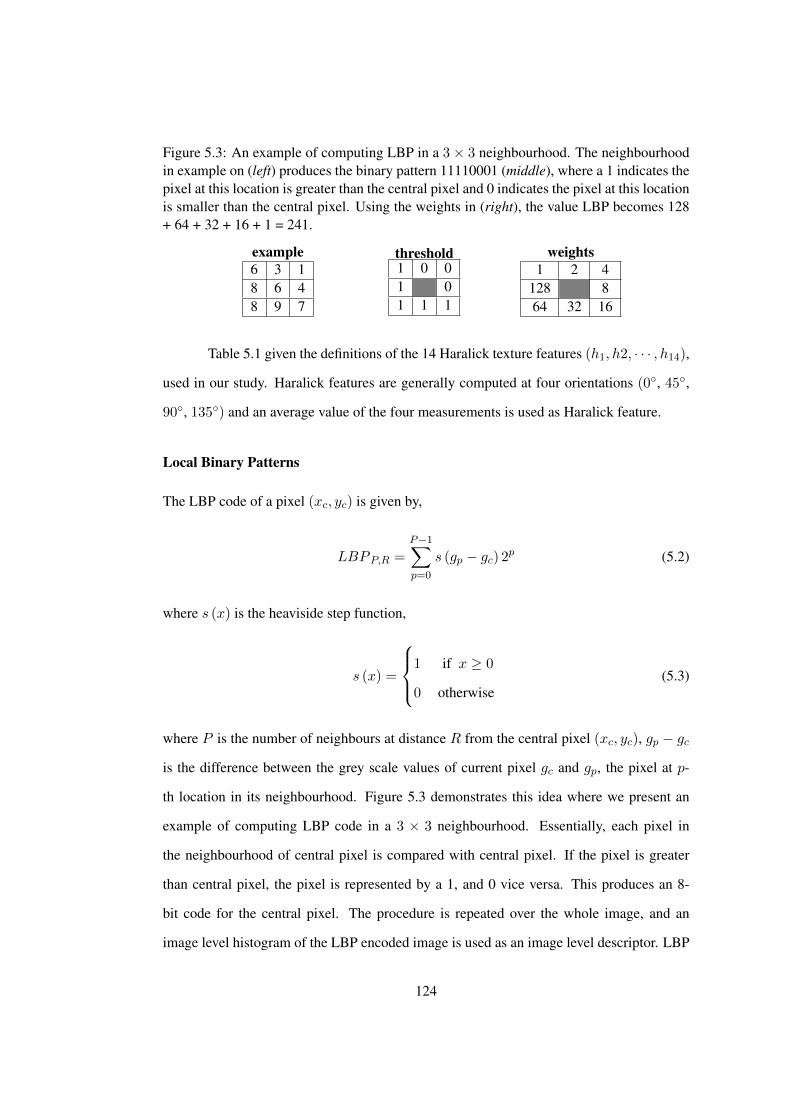
Figure 5.3: An example of computing LBP in a 3× 3 neighbourhood. The neighbourhoodin example on (left) produces the binary pattern 11110001 (middle), where a 1 indicates thepixel at this location is greater than the central pixel and 0 indicates the pixel at this locationis smaller than the central pixel. Using the weights in (right), the value LBP becomes 128+ 64 + 32 + 16 + 1 = 241.

example6 3 18 6 48 9 7

threshold1 0 01 01 1 1

weights1 2 4

128 864 32 16

Table 5.1 given the definitions of the 14 Haralick texture features (h1, h2, · · · , h14),

used in our study. Haralick features are generally computed at four orientations (0◦, 45◦,

90◦, 135◦) and an average value of the four measurements is used as Haralick feature.

Local Binary Patterns

The LBP code of a pixel (xc, yc) is given by,

LBPP,R =P−1∑

p=0

s (gp − gc) 2p (5.2)

where s (x) is the heaviside step function,

s (x) =

1 if x ≥ 0

0 otherwise(5.3)

where P is the number of neighbours at distance R from the central pixel (xc, yc), gp − gcis the difference between the grey scale values of current pixel gc and gp, the pixel at p-

th location in its neighbourhood. Figure 5.3 demonstrates this idea where we present an

example of computing LBP code in a 3 × 3 neighbourhood. Essentially, each pixel in

the neighbourhood of central pixel is compared with central pixel. If the pixel is greater

than central pixel, the pixel is represented by a 1, and 0 vice versa. This produces an 8-

bit code for the central pixel. The procedure is repeated over the whole image, and an

image level histogram of the LBP encoded image is used as an image level descriptor. LBP

124

is a very popular texture descriptor and is widely used in various applications including

face recognition [249, 250], object categorisation [251], image classification [252, 253] and

histologic texture classification [254, 255, 256].

5.1.2 Feature Normalisation and Selection

Features computed in the step 5.1.1 possess different dynamic ranges of feature values. Us-

ing such features in a machine learning framework may hamper the performance of pattern

classifiers, as most of the machine learning frameworks employ the distance between pairs

of feature vectors as a measure of similarity/disimilarity. If the range of feature values is

very large in one feature, say in the range of several thousands, and very small in another

feature, say in the range of less than 1, the decision boundary learned by the classifier will

be highly influenced by the former feature. Therefore, in general, features are scaled be-

tween some predefined range before feeding them to a classifier. We normalise the range of

features as follows,

f i =f i − f imin

f imax − f imin(5.4)

where f i and f i refer to the i-th feature before and after normalisation, and f imin and f imax

refer to the minimum and maximum values of i-th feature. Note that feature normalisation

is performed at each feature level. Feature selection is then performed to remove features

that are highly correlated with each other or if some features remain constant throughout the

dataset. We further employ Fisher criteria [257] to rank the remaining features according

to some univariate metric and select the highest ranking features. The ranking of features

reflects the discriminative power of each feature.

$i =

(µi(+) − µi(−)

)2

(σi(+)

)2+(σi(−)

)2 (5.5)

where$i is the relative importance of i-th feature in discriminating positive examples from

negative examples, µi(+) and µi(−) is the mean of positive and negative examples,(σi(+)

)

125

and(σi(−)

)are the standard deviations of the positive and negative examples.

5.1.3 Classification

This section presents a brief overview of the types of classifiers used for scoring nuclear

atypia. We use three widely used paradigms for multi-class classification: decision trees,

nearest neighbours, and discriminant classifiers [258]. In decision tree paradigm, we eval-

uate decision tree and RUSBoost classifiers, whereas in discriminant classifiers paradigm,

we evaluate linear and quadratic discriminant classifiers. Following subsections briefly de-

scribe each paradigm.

Decision Trees

Decision tree (DT) is a non-linear, supervised predictive model of learning that maps fea-

tures to class labels using a tree-like structure [259]. The idea is to iteratively split variables

into groups, evaluate homogeneity within each group and continue to split again if neces-

sary until a desired level of homogeneity is achieved or the groups are small enough to be

further divided. Homogeneity is generally determined using three well known measures:

Gini’s diversity index, deviance and twoing [260, 261]. Classification of an unknown sam-

ple using decision tree involves the traversal of tree - from the root node down to a leaf

node, where the leaf node contains the class labels.

Most statistical machine learning algorithms when trained on highly skewed datasets

(data in which various classes are unevenly represented), build a prediction model that

favours the majority class. This class-imbalance problem is common in medical datasets

including MITOS-Atypia dataset where score-2 nuclear atypia images dominate (≈ 75%)

the other 2 scores (≈ 17% and ≈ 8%). Boosting [262] and sampling [263] strategies are

generally employed to overcome this problem. In boosting, the idea is to take a large num-

ber of weak classifiers (decision trees, regression models), weigh and add them up to get

a strong classifier. Weights are learned in an iterative manner by minimising an objective

function on training data. During each iteration, weights are updated with the goal of cor-

126

rectly classifying training data in the next iteration that are incorrectly classified during the

current iteration. Sampling strategies balance the distribution of classes in the training data

by either oversampling the minority class or undersampling the majority class. RUSBoost

(or Robust UnderSampling and Boosting) is an algorithm that combines undersampling

and boosting to alleviate this problem [264] and has proved to be very successful in various

applications especially under the conditions where the data is skewed [265, 266, 267].

k-Nearest Neighbour Classifier

k-Nearest neighbour classifiers belong to a class of non-parametric classification tech-

niques. The method classifies a given object based on the majority vote of its k nearest

neighbours in the training dataset. Distance between neighbours is usually computed using

the Euclidean metric. Typical values of k are 1, 3, 5. An odd value of k is preferred so as

to avoid draw while voting of neighbours.

Linear and quadratic Classifiers

Linear and quadratic classifiers are widely used in machine learning and statistical classi-

fication. These classifiers transform the data such that the two (or more) classes are more

discriminant in the transform domain. Both linear and quadratic transformations (func-

tions) can be employed for this propose - hence the names linear and quadratic discriminate

classifiers. A linear classifier achieves this by making a classification decision based on

the value of a linear combination of the features whereas a quadratic classifier separates

measurements of two or more classes of objects or events by a quadric surface. We evaluate

both types of classifiers to perform nuclear atypia scoring.

5.2 The Proposed Framework

Figure 5.4 presents the proposed framework for image classification using the RC and the

mSPD descriptors. An image is divided into small non-overlapping regions. For each re-

127

)

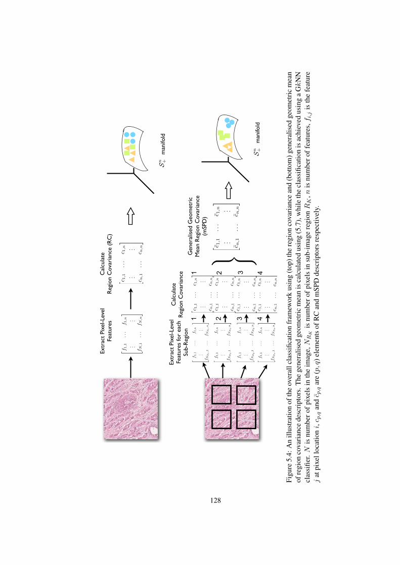
Extr

act

Pixe

l-Lev

el !

Feat

ures

for

each

Su

b-R

egio

n

Cal

cula

te !

Reg

ion

Cov

aria

nce

Sn +m

anifo

ld

Extr

act

Pixe

l-Lev

el !

Feat

ures

2 6 4f 1

,1..

.f 1

,n

. . .. . .

f N,1

...

f N,n

3 7 5

Cal

cula

te !

Reg

ion

Cov

aria

nce

(RC

)

Sn +m

anifo

ld

11 2

2 33

44

2 6 4c 1,1

...

c 1,n

. . .. . .

c n,1

...

c n,n

3 7 5

2 6 4c 1,1

...

c 1,n

. . .. . .

c n,1

...

c n,n

3 7 52 6 4c 1

,1..

.c 1

,n

. . .. . .

c n,1

...

c n,n

3 7 52 6 4c 1

,1..

.c 1

,n

. . .. . .

c n,1

...

c n,n

3 7 52 6 4c 1

,1..

.c 1

,n

. . .. . .

c n,1

...

c n,n

3 7 5

2 6 4c 1,1

...

c 1,n

. . .. . .

c n,1

...

c n,n

3 7 5

2 6 4f 1

,1..

.f 1

,n

. . .. . .

f NR

1,1

...

f NR

1,n

3 7 5

2 6 4f 1

,1..

.f 1

,n

. . .. . .

f NR

2,1

...

f NR

2,n

3 7 5

2 6 4f 1

,1..

.f 1

,n

. . .. . .

f NR

3,1

...

f NR

3,n

3 7 5

2 6 4f 1

,1..

.f 1

,n

. . .. . .

f NR

4,1

...

f NR

4,n

3 7 5

Gen

eral

ised

Geo

met

ric!

Mea

n R

egio

n C

ovar

ianc

e!(m

SPD

)

Figu

re5.

4:A

nill

ustr

atio

nof

the

over

allc

lass

ifica

tion

fram

ewor

kus

ing

(top

)the

regi

onco

vari

ance

and

(bot

tom

)gen

eral

ised

geom

etri

cm

ean

ofre

gion

cova

rian

cede

scri

ptor

s.T

hege

nera

lised

geom

etri

cm

ean

isca

lcul

ated

usin

g(5

.7),

whi

leth

ecl

assi

ficat

ion

isac

hiev

edus

ing

aGk

NN

clas

sifie

r.N

isnu

mbe

rofp

ixel

sin

the

imag

e,NRK

isnu

mbe

rofp

ixel

sin

sub-

imag

ere

gionRK

,nis

num

bero

ffea

ture

s,f i,j

isth

efe

atur

ej

atpi

xell

ocat

ioni,c p,q

andc p,q

are

(p,q

)ele

men

tsof

RC

and

mSP

Dde

scri

ptor

sre

spec

tivel

y.

128

gion, pixel level features are collected to form an RC descriptor. RC descriptors of different

regions are then summarised into a single mSPD descriptor, by calculating the generalised

geometric mean of RC descriptors. A GkNN classifier, which utilises the known structure

of the Riemannian manifold of SPD matrices, is then employed to assign the nuclear atypia

scores (1, 2 or 3) to test images.

In the following subsections, we first describe the RC and mSPD descriptors fol-

lowed by the description of GkNN classifier along with various distance metrics used for

computing geodesic distance. Finally, we present a description of the kernel trick that

is employed to circumvent the computational performance issues that arise by employing

computationally intensive geodesic distance metrics.

5.2.1 The Region Covariance Descriptor

The region covariance (RC) descriptor initially proposed by Tuzel et al. [39] has emerged

in recent years as a powerful yet simple way to represent image contents in an efficient

manner. The RC descriptor can be computed by first characterising an image I with a set of

pixel level n-dimensional features f(x, y) = {f1(x, y), f2(x, y), . . . , fn(x, y)} for all (x, y)

image coordinates. These pixel level characterisations may either be intensity values (red,

green, blue, grey), gradients, Hessian or filter responses. If {fi}i=1···n is the n-dimensional

features inside the image I with N pixels, the RC descriptor can be represented as ,

C =1

n− 1

n∑

i=1

(fi − µ) (fi − µ)T (5.6)

where C is the n× n covariance matrix, and µ is the mean of the data points.

The RC descriptors have some desirable properties. For instance, as the diagonal

entries of the covariance matrix represent the variance of each feature and non-diagonal

entries are the respective correlations, RC descriptor provides a succinct way of aggregating

features that might be correlated. If the features are carefully chosen, these descriptors

may be invariant to rotations, scales and illuminations mainly because the descriptor is

129

independent of the number of points in the region, and ordering of the points. The RC

descriptor is a relatively low dimensional descriptor as the size N of the region is generally

much higher than the dimensionality n of the features. Moreover, due to symmetric property

of SPD matrices, only n(n+1)2 different values are effective, which further decreases the size

of the descriptor.

The RC descriptors have been demonstrated to achieve state-of-the-art performance

in many computer vision tasks, including face recognition [131, 132], pedestrian detection

[268, 269], tracking [270], texture classification [39, 271]. Recently, it has been used for

medical image analysis by Keskin et al. [272] for classification of culture cancer cells.

Nonetheless, their analysis does not utilise the differential geometry structure of the RC

descriptor.

5.2.2 Generalised Geometric Mean of Symmetric Positive Definite Matrices

as an Image Descriptor

The idea of covariance descriptors has been quite successful in representing regional con-

tents for the purposes of object detection and tracking [268, 269, 270]. A major assumption

in using this idea, however, for image level classification is that the image contains more or

less homogeneous contents. This assumption does not hold true in our application, where

heterogeneity of tumour micro-environment plays a major role in non-homogeneous nature

of various parts of the tissue specimen [273].

We address this limitation by proposing an image descriptor that divides an image

into sub-regions, calculates an RC descriptor for each sub-region, and combines the region

level RC descriptors to generate an image level descriptor. More specifically, an image I

is divided into K small non-overlapping sub-regions {R1, ..., RK} and an RC descriptor

is computed in each sub-region CRk , k = 1, ...,K using (5.6). The set of RC descriptors

from a single image are SPDs that can be considered as a set of points on a Riemannian

manifoldM and, therefore, a generalised geometric mean of these points can be computed

using the Frechet mean of the RC descriptors [274, 275].

130

Frechet mean is the point X on the manifoldM that minimises the sum of squared

Riemannian distances to all the points CRk on M. The value of Frechet function at a

random point CRk is the expected square distance from CRk to X. Using this definition,

an empirical estimate of the Frechet mean given a collection of observations (CRk ) on the

manifoldM can be given by,

M(I) = argminX∈M

K∑

k=1

dist2(X,CRk), (5.7)

where dist(·, ·) is the distance metric on M, and M is the space of SPD matrices. Note

that equation (5.7) is generic, e.g., ifM is a Eucidean space equipped with the usual Eu-

clidean distance, this equation calculates arithmetic mean. The Frechet mean is calculated

by performing optimisation of (5.7), using the Riemannian Trust-Region solver [276].

The mean covariance matrix calculated in this way is the generalised geometric

mean and is, therefore, a representative of potentially different covariance matrices calcu-

lated from heterogeneous sub-regions of each image. The mean covariance matrices are

themselves SPD matrices, which form a space of SPD matrices (S+n ) with each point in

this space representing an image level covariance descriptor generated by calculating the

generalised geometric mean of several sub-region level covariance matrices.

5.2.3 Nearest Neighbour Classification on Riemannian Manifold of Symmet-

ric Positive Definite Matrices

An n×nmSPD is a member of the space S+n of n×n SPD matrices, which is an open con-

vex subset of the Euclidean space. However, S+n is not a vector space with usual addition

and scalar multiplication as, for example, it is not closed under negative scalar multiplica-

tion. Analysing SPD matrices under usual Euclidean geometry would fail to capture the

nonlinearity of S+n . Therefore, the space S+

n of n × n SPD matrices is mostly studied

when endowed with Riemannian metric and thus forms a Riemannian manifold [40]. In

131

such a case, geodesic distance1 induced by Riemannian metric is a more natural measure of

distance than the Euclidean distance.

A number of metrics on the space of S+n have been recently proposed, not all of

them induce a true geodesic distance. The two most widely used distance measures are the

affine-invariant distance [40] and the log-Euclidean distance [277]. The main reason for

their popularity is that they induce the true geodesic distance by a Riemannian metrics. In

fact, S+n forms a Riemannian manifold with negative curvature when endowed by affine

invariant metric [40], and a Riemannian manifold with null curvature when endowed by the

log-Euclidean metric [277].

Kernel methods are commonly used in machine learning and computer vision areas

to explore non-linear structures present in the data. The basic idea of kernel methods is to

map the input data to a high-dimensional feature space to obtain a richer representation of

data distribution. This basic idea can be translated to generalised non-linear manifolds as

well. Jayasumana et al. [278] present a framework that maps a point on a non-linear man-

ifold S+n using the so-called Stein kernel. In this chapter, we compute geodesic distances

based on affine-invariant, log-Euclidean and Stein kernel metric due to the Riemannian

manifold structure of the space of SPD matrices.

Assume X,Y ∈ S+n are two SPD matrices. Then, following list gives a brief

overview of the distance measures used in this chapter.

• Affine-invariant metric Affine invariant metric calculates distance between two

SPDs lying on a Riemannian manifold [40, 279, 280] using,

dist(X,Y) = ‖log(X−1/2YX−1/2)‖F= ‖log(Y−1/2XY−1/2)‖F (5.8)

where ‖·‖F denotes the Frobenius norm and log(·) denotes the matrix logarithm.

1Geodesic distance between two points on a manifold is the length of the shortest curve connecting the twopoints.

132

Pennec et al. [40] provide a closed form solution to this equation,

dist(X,Y) =n∑

i=1

(Log(vi))2 (5.9)

where vi are the eigenvalues of the product X−1/2YX−1/2, Log(·) denotes the usual

element logarithm, and n is the number of diagonal elements in the eigenvalue matrix.

• Log-Euclidean metric Log-Euclidean metric uses logarithmic mapping to map the

points (X and Y) lying on the Riemannian manifold S+n to the Euclidean space

[277]. Once the points are mapped to the Euclidean space, standard Euclidean norm

is computed to calculate the distance between the two points.

dist(X,Y) = ‖log(X)− log(Y)‖F= ‖log(Y)− log(X)‖F (5.10)

where log(·) denotes matrix logarithm.

• Positive definite kernel Computation of geodesic distance in equations (5.8) and

(5.10) involves nonlinear log operator which can result in nontrivial numerical bur-

den. Motivated by this fact, we employ a kernel-based approach which defines an

embedding function φ : S+n → H in order to map the SPD matrices into the high-

dimensional reproducing kernel Hilbert space (RKHS) H. Since the RKHS is an

inner product space, dissimilarity measure between two points φ(X), φ(Y) ∈ H for

any X,Y ∈ S+n can simply be calculated by their inner product which is defined in

the form of a positive definite kernel k(X,Y) : S+n × S+

n → R [281],

k(X,Y) = e−σS(X,Y) (5.11)

where σ ∈ {12 ,

22 , ...,

n−12 } ∪ {τ ∈ R : τ > n−1

2 } is a scaling factor, and

S(X,Y) ≡ log

(det

(X + Y

2

))− 1

2log (det (XY)) (5.12)

133

is a symmetric Stein divergence which behaves similarly to geodesic distance as in

(5.8) induced by affine-invariant metric within a tight bound [281], and det(·) is the

determinant operator. Positive-definite kernel distance (5.11) behaves similar to the

true geodesic distance in the GkNN classifier. The value of the kernel function ranges

between 0 and 1. The higher the value of the kernel function, the smaller the distance

between the two SPD matrices.

GkNN performs nearest neighbour classification similar to standard kNN classi-

fication. The only difference is that in standard kNN classification, Euclidean distances

between two points are used to find the k-nearest neighbours. However, in case of GkNN,

geodesic distances induced by affine-invariant metric (5.8), log-Euclidean metric (5.10) or

Stein kernel (5.11) will be used instead. Since GkNN classifier explicitly exploits the struc-

ture of Riemannian manifold of SPD matrices through the use of geodesic distances, we

expect superior performance.

5.3 Experimental Results and Discussion

We perform all experiments on the publicly available MITOS-Atypia dataset2, which com-

prises of 297 breast histology images extracted from 11 patients, and is part of an ongoing

Mitos-Atypia challenge. Details about the dataset can be found in Section 1.6. Following

subsections present the results of various experiments conducted to evaluate performance

of the proposed nuclear atypia scoring framework.

5.3.1 Comparison of the Baseline and the Proposed Frameworks

For computation of the RC and mSPD descriptors, texture features are calculated by apply-

ing the maximum response (MR8) filter bank [282] on the greyscale image. The MR8 filter

bank consists of 38 filters: 2 isotropic filters (Gaussian and a Laplacian of Gaussian), an

edge filter at 3 scales and 6 orientations and a bar filter at 3 scales and 6 orientations. At2http://mitos-atypia-14.comicframework.org/

134

each scale, only the maximum response across all 6 orientations of edge and bar filters is

measured which reduces the number of responses from 12 (6 responses for edge filters and

6 responses for bar filters) to 2 (1 response for edge filter and 1 response for bar filters). This

generates 6 edge and bar filter responses at 3 scales. Adding two isotropic filter responses

to this set produces 8 filter responses on the whole. Figure 5.5 shows the response of MR8

filter bank on a sample image from MITOS-Atypia dataset.

In order to compute covariance descriptors (both RC and mSPD), we append L,

a, b and BR intensities along with the 8 texture filter responses to generate a 12 × 12

covariance matrix. The number of nearest neighbours are fixed to 5 for both Euclidean

and geodesic nearest neighbour algorithms. In order to perform classification on classical

machine learning techniques (decision trees (DT), RUSBoost, kNN, linear discriminant

analysis (LDA) and quadratic discriminant analysis (QDA)), SPD matrices are mapped to

high dimensional Euclidean space. This mapping is also referred to as flattening of the

manifold in the literature [277, 278, 281]. Since SPD matrices are symmetric, therefore we

use n(n+1)2 different values of the matrix as input feature vector to the classical machine

learning techniques.

In order to keep the comparison fair, we compute baseline features on greyscale

images as well. For baseline LBP features, we compute 59-bin LBP histogram descriptor

which is in line with the number of bins suggested by Heikkila & Ahonen [249]. For

computation of 14 Haralick features, we use 5 displacements (1, 2, . . . , 5) and concatenate

the 14 descriptors from each displacement to generate a 70-dimensional Haralick descriptor

for each image. In all our experiments, we perform 5-fold cross validation. Moreover, each

experiment is repeated 10 times and average accuracies are reported.

Tables 5.2 and 5.3 show the experimental results for nuclear atypia subtypes classi-

fication using the baseline and the proposed nuclear atypia scoring frameworks respectively.

We observe in Table 5.2 that classical texture descriptors like LBP and Haralick do not per-

form well for the task of nuclear atypia scoring in BC histopathology images as compared

to RC and mSPD descriptors, even if a mix of complementary texture features are used

135

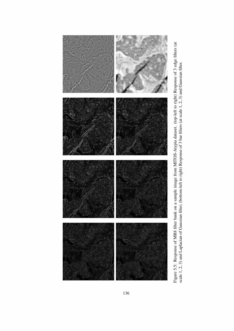
Figu

re5.

5:R

espo

nse

ofM

R8

filte

rba

nkon

asa

mpl

eim

age

from

MIT

OS-

Aty

pia

data

set.

(top

-lef

tto

righ

t)R

espo

nse

of3

edge

filte

rs(a

tsc

ale

1,2,

3)an

dL

apla

cian

ofG

auss

ian

filte

r;(b

otto

m-l

eftt

ori

ght)

Res

pons

eof

3ba

rfilte

rs(a

tsca

le1,

2,3)

and

Gau

ssia

nfil

ter.

136

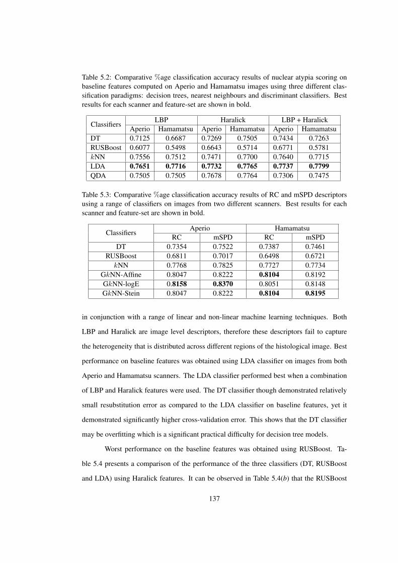
Table 5.2: Comparative %age classification accuracy results of nuclear atypia scoring onbaseline features computed on Aperio and Hamamatsu images using three different clas-sification paradigms: decision trees, nearest neighbours and discriminant classifiers. Bestresults for each scanner and feature-set are shown in bold.

ClassifiersLBP Haralick LBP + Haralick

Aperio Hamamatsu Aperio Hamamatsu Aperio HamamatsuDT 0.7125 0.6687 0.7269 0.7505 0.7434 0.7263RUSBoost 0.6077 0.5498 0.6643 0.5714 0.6771 0.5781kNN 0.7556 0.7512 0.7471 0.7700 0.7640 0.7715LDA 0.7651 0.7716 0.7732 0.7765 0.7737 0.7799QDA 0.7505 0.7505 0.7678 0.7764 0.7306 0.7475

Table 5.3: Comparative %age classification accuracy results of RC and mSPD descriptorsusing a range of classifiers on images from two different scanners. Best results for eachscanner and feature-set are shown in bold.

ClassifiersAperio Hamamatsu

RC mSPD RC mSPDDT 0.7354 0.7522 0.7387 0.7461

RUSBoost 0.6811 0.7017 0.6498 0.6721kNN 0.7768 0.7825 0.7727 0.7734

GkNN-Affine 0.8047 0.8222 0.8104 0.8192GkNN-logE 0.8158 0.8370 0.8051 0.8148GkNN-Stein 0.8047 0.8222 0.8104 0.8195

in conjunction with a range of linear and non-linear machine learning techniques. Both

LBP and Haralick are image level descriptors, therefore these descriptors fail to capture

the heterogeneity that is distributed across different regions of the histological image. Best

performance on baseline features was obtained using LDA classifier on images from both

Aperio and Hamamatsu scanners. The LDA classifier performed best when a combination

of LBP and Haralick features were used. The DT classifier though demonstrated relatively

small resubstitution error as compared to the LDA classifier on baseline features, yet it

demonstrated significantly higher cross-validation error. This shows that the DT classifier

may be overfitting which is a significant practical difficulty for decision tree models.

Worst performance on the baseline features was obtained using RUSBoost. Ta-

ble 5.4 presents a comparison of the performance of the three classifiers (DT, RUSBoost

and LDA) using Haralick features. It can be observed in Table 5.4(b) that the RUSBoost

137

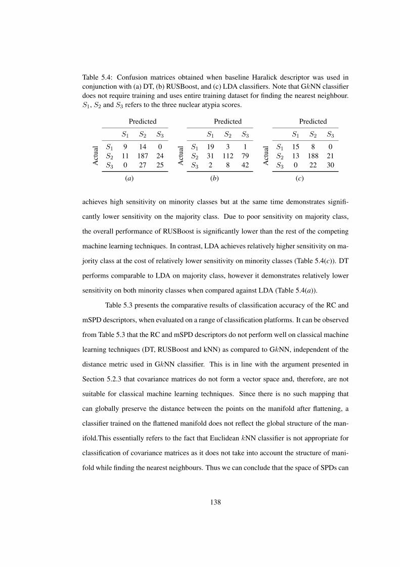
Table 5.4: Confusion matrices obtained when baseline Haralick descriptor was used inconjunction with (a) DT, (b) RUSBoost, and (c) LDA classifiers. Note that GkNN classifierdoes not require training and uses entire training dataset for finding the nearest neighbour.S1, S2 and S3 refers to the three nuclear atypia scores.

Predicted

S1 S2 S3

S1 9 14 0S2 11 187 24

Act

ual

S3 0 27 25

Predicted

S1 S2 S3

S1 19 3 1S2 31 112 79

Act

ual

S3 2 8 42

Predicted

S1 S2 S3

S1 15 8 0S2 13 188 21

Act

ual

S3 0 22 30

(a) (b) (c)

achieves high sensitivity on minority classes but at the same time demonstrates signifi-

cantly lower sensitivity on the majority class. Due to poor sensitivity on majority class,

the overall performance of RUSBoost is significantly lower than the rest of the competing

machine learning techniques. In contrast, LDA achieves relatively higher sensitivity on ma-

jority class at the cost of relatively lower sensitivity on minority classes (Table 5.4(c)). DT

performs comparable to LDA on majority class, however it demonstrates relatively lower

sensitivity on both minority classes when compared against LDA (Table 5.4(a)).

Table 5.3 presents the comparative results of classification accuracy of the RC and

mSPD descriptors, when evaluated on a range of classification platforms. It can be observed

from Table 5.3 that the RC and mSPD descriptors do not perform well on classical machine

learning techniques (DT, RUSBoost and kNN) as compared to GkNN, independent of the

distance metric used in GkNN classifier. This is in line with the argument presented in

Section 5.2.3 that covariance matrices do not form a vector space and, therefore, are not

suitable for classical machine learning techniques. Since there is no such mapping that

can globally preserve the distance between the points on the manifold after flattening, a

classifier trained on the flattened manifold does not reflect the global structure of the man-

ifold.This essentially refers to the fact that Euclidean kNN classifier is not appropriate for

classification of covariance matrices as it does not take into account the structure of mani-

fold while finding the nearest neighbours. Thus we can conclude that the space of SPDs can

138

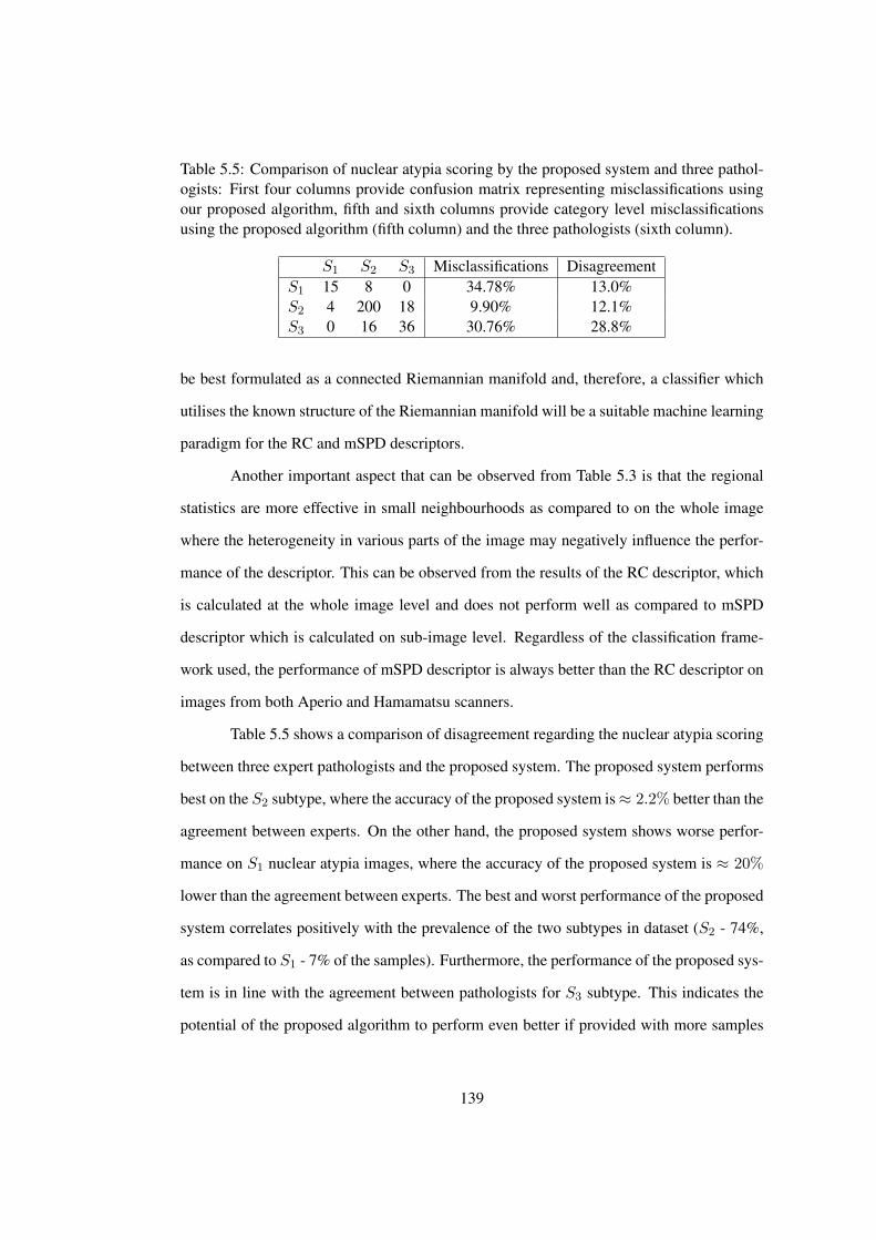
Table 5.5: Comparison of nuclear atypia scoring by the proposed system and three pathol-ogists: First four columns provide confusion matrix representing misclassifications usingour proposed algorithm, fifth and sixth columns provide category level misclassificationsusing the proposed algorithm (fifth column) and the three pathologists (sixth column).

S1 S2 S3 Misclassifications DisagreementS1 15 8 0 34.78% 13.0%S2 4 200 18 9.90% 12.1%S3 0 16 36 30.76% 28.8%

be best formulated as a connected Riemannian manifold and, therefore, a classifier which

utilises the known structure of the Riemannian manifold will be a suitable machine learning

paradigm for the RC and mSPD descriptors.

Another important aspect that can be observed from Table 5.3 is that the regional

statistics are more effective in small neighbourhoods as compared to on the whole image

where the heterogeneity in various parts of the image may negatively influence the perfor-

mance of the descriptor. This can be observed from the results of the RC descriptor, which

is calculated at the whole image level and does not perform well as compared to mSPD

descriptor which is calculated on sub-image level. Regardless of the classification frame-

work used, the performance of mSPD descriptor is always better than the RC descriptor on

images from both Aperio and Hamamatsu scanners.

Table 5.5 shows a comparison of disagreement regarding the nuclear atypia scoring

between three expert pathologists and the proposed system. The proposed system performs

best on the S2 subtype, where the accuracy of the proposed system is≈ 2.2% better than the

agreement between experts. On the other hand, the proposed system shows worse perfor-

mance on S1 nuclear atypia images, where the accuracy of the proposed system is ≈ 20%

lower than the agreement between experts. The best and worst performance of the proposed

system correlates positively with the prevalence of the two subtypes in dataset (S2 - 74%,

as compared to S1 - 7% of the samples). Furthermore, the performance of the proposed sys-

tem is in line with the agreement between pathologists for S3 subtype. This indicates the

potential of the proposed algorithm to perform even better if provided with more samples

139

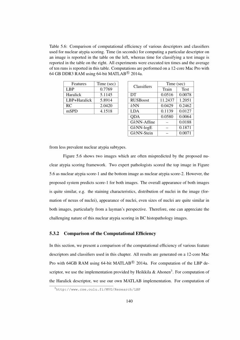
Table 5.6: Comparison of computational efficiency of various descriptors and classifiersused for nuclear atypia scoring. Time (in seconds) for computing a particular descriptor onan image is reported in the table on the left, whereas time for classifying a test image isreported in the table on the right. All experiments were executed ten times and the averageof ten runs is reported in this table. Computations are performed on a 12-core Mac Pro with64 GB DDR3 RAM using 64-bit MATLAB R© 2014a.

Features Time (sec)Classifiers

Time (sec)LBP 0.7769 Train TestHaralick 5.1145 DT 0.0516 0.0078LBP+Haralick 5.8914 RUSBoost 11.2437 1.2051RC 2.0420 kNN 0.0429 0.2462mSPD 4.1518 LDA 0.1139 0.0127

QDA 0.0580 0.0064GkNN-Affine – 0.0188GkNN-logE – 0.1871GkNN-Stein – 0.0071

from less prevalent nuclear atypia subtypes.

Figure 5.6 shows two images which are often mispredicted by the proposed nu-

clear atypia scoring framework. Two expert pathologists scored the top image in Figure

5.6 as nuclear atypia score-1 and the bottom image as nuclear atypia score-2. However, the

proposed system predicts score-1 for both images. The overall appearance of both images

is quite similar, e.g. the staining characteristics, distribution of nuclei in the image (for-

mation of nexus of nuclei), appearance of nuclei, even sizes of nuclei are quite similar in

both images, particularly from a layman’s perspective. Therefore, one can appreciate the

challenging nature of this nuclear atypia scoring in BC histopathology images.

5.3.2 Comparison of the Computational Efficiency

In this section, we present a comparison of the computational efficiency of various feature

descriptors and classifiers used in this chapter. All results are generated on a 12-core Mac

Pro with 64GB RAM using 64-bit MATLAB R© 2014a. For computation of the LBP de-

scriptor, we use the implementation provided by Heikkila & Ahonen3. For computation of

the Haralick descriptor, we use our own MATLAB implementation. For computation of3http://www.cse.oulu.fi/MVG/Research/LBP

140

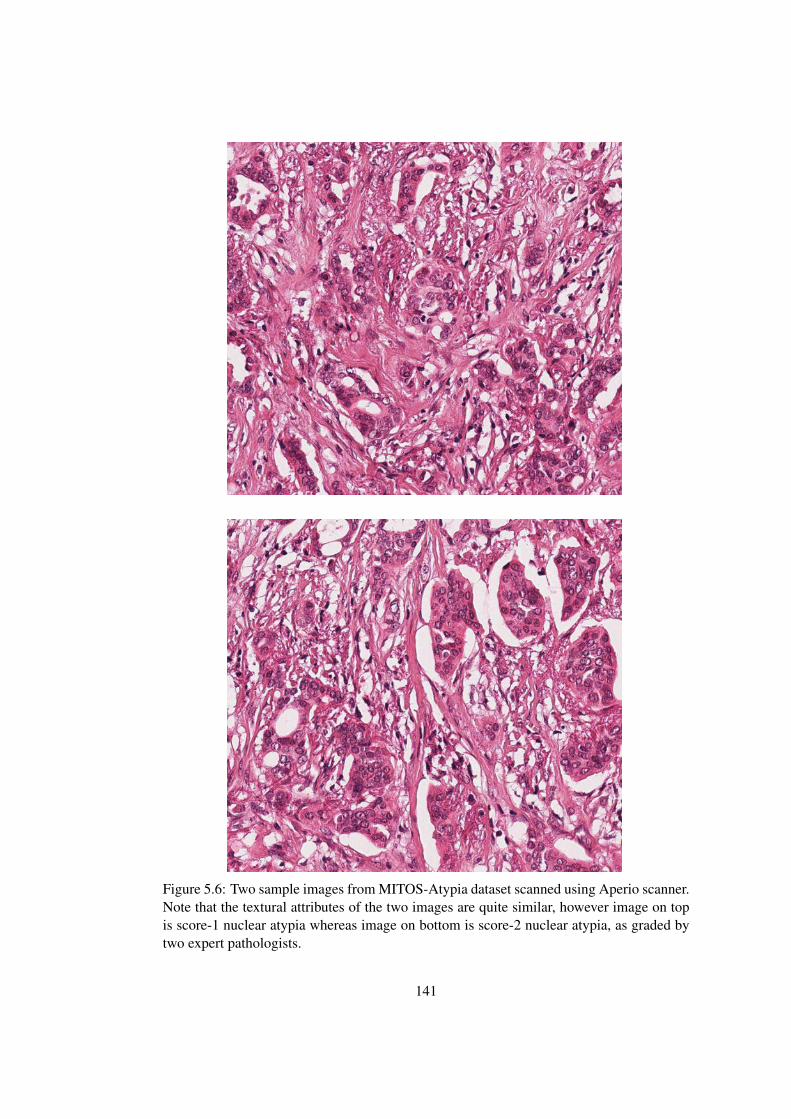
Figure 5.6: Two sample images from MITOS-Atypia dataset scanned using Aperio scanner.Note that the textural attributes of the two images are quite similar, however image on topis score-1 nuclear atypia whereas image on bottom is score-2 nuclear atypia, as graded bytwo expert pathologists.

141

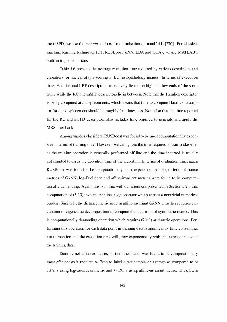
the mSPD, we use the manopt toolbox for optimisation on manifolds [276]. For classical

machine learning techniques (DT, RUSBoost, kNN, LDA and QDA), we use MATLAB’s

built-in implementations.

Table 5.6 presents the average execution time required by various descriptors and

classifiers for nuclear atypia scoring in BC histopathology images. In terms of execution

time, Haralick and LBP descriptors respectively lie on the high and low ends of the spec-

trum, while the RC and mSPD descriptors lie in between. Note that the Haralick descriptor

is being computed at 5 displacements, which means that time to compute Haralick descrip-

tor for one displacement should be roughly five times less. Note also that the time reported

for the RC and mSPD descriptors also includes time required to generate and apply the

MR8 filter bank.

Among various classifiers, RUSBoost was found to be most computationally expen-

sive in terms of training time. However, we can ignore the time required to train a classifier

as the training operation is generally performed off-line and the time incurred is usually

not counted towards the execution time of the algorithm. In terms of evaluation time, again

RUSBoost was found to be computationally most expensive. Among different distance

metrics of GkNN, log-Euclidean and affine-invariant metrics ware found to be computa-

tionally demanding. Again, this is in line with our argument presented in Section 5.2.3 that

computation of (5.10) involves nonlinear log operator which carries a nontrivial numerical

burden. Similarly, the distance metric used in affine-invariant GkNN classifier requires cal-

culation of eigenvalue decomposition to compute the logarithm of symmetric matrix. This

is computationally demanding operation which requires O(n3) arithmetic operations. Per-

forming this operation for each data point in training data is significantly time consuming,

not to mention that the execution time will grow exponentially with the increase in size of

the training data.

Stein kernel distance metric, on the other hand, was found to be computationally

most efficient as it requires ≈ 7ms to label a test sample on average as compared to ≈

187ms using log-Euclidean metric and ≈ 19ms using affine-invariant metric. Thus, Stein

142

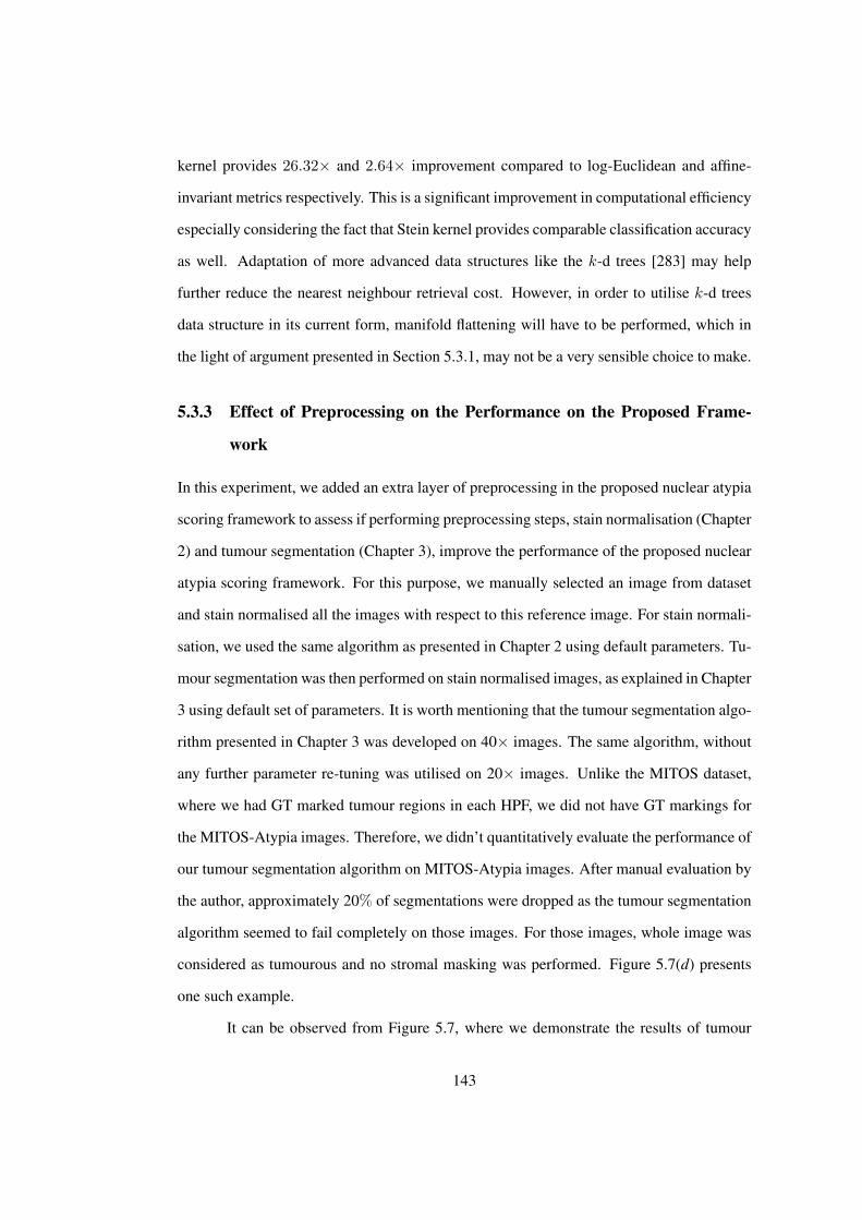
kernel provides 26.32× and 2.64× improvement compared to log-Euclidean and affine-

invariant metrics respectively. This is a significant improvement in computational efficiency

especially considering the fact that Stein kernel provides comparable classification accuracy

as well. Adaptation of more advanced data structures like the k-d trees [283] may help

further reduce the nearest neighbour retrieval cost. However, in order to utilise k-d trees

data structure in its current form, manifold flattening will have to be performed, which in

the light of argument presented in Section 5.3.1, may not be a very sensible choice to make.

5.3.3 Effect of Preprocessing on the Performance on the Proposed Frame-

work

In this experiment, we added an extra layer of preprocessing in the proposed nuclear atypia

scoring framework to assess if performing preprocessing steps, stain normalisation (Chapter

2) and tumour segmentation (Chapter 3), improve the performance of the proposed nuclear

atypia scoring framework. For this purpose, we manually selected an image from dataset

and stain normalised all the images with respect to this reference image. For stain normali-

sation, we used the same algorithm as presented in Chapter 2 using default parameters. Tu-

mour segmentation was then performed on stain normalised images, as explained in Chapter

3 using default set of parameters. It is worth mentioning that the tumour segmentation algo-

rithm presented in Chapter 3 was developed on 40× images. The same algorithm, without

any further parameter re-tuning was utilised on 20× images. Unlike the MITOS dataset,

where we had GT marked tumour regions in each HPF, we did not have GT markings for

the MITOS-Atypia images. Therefore, we didn’t quantitatively evaluate the performance of

our tumour segmentation algorithm on MITOS-Atypia images. After manual evaluation by

the author, approximately 20% of segmentations were dropped as the tumour segmentation

algorithm seemed to fail completely on those images. For those images, whole image was

considered as tumourous and no stromal masking was performed. Figure 5.7(d) presents

one such example.

It can be observed from Figure 5.7, where we demonstrate the results of tumour

143

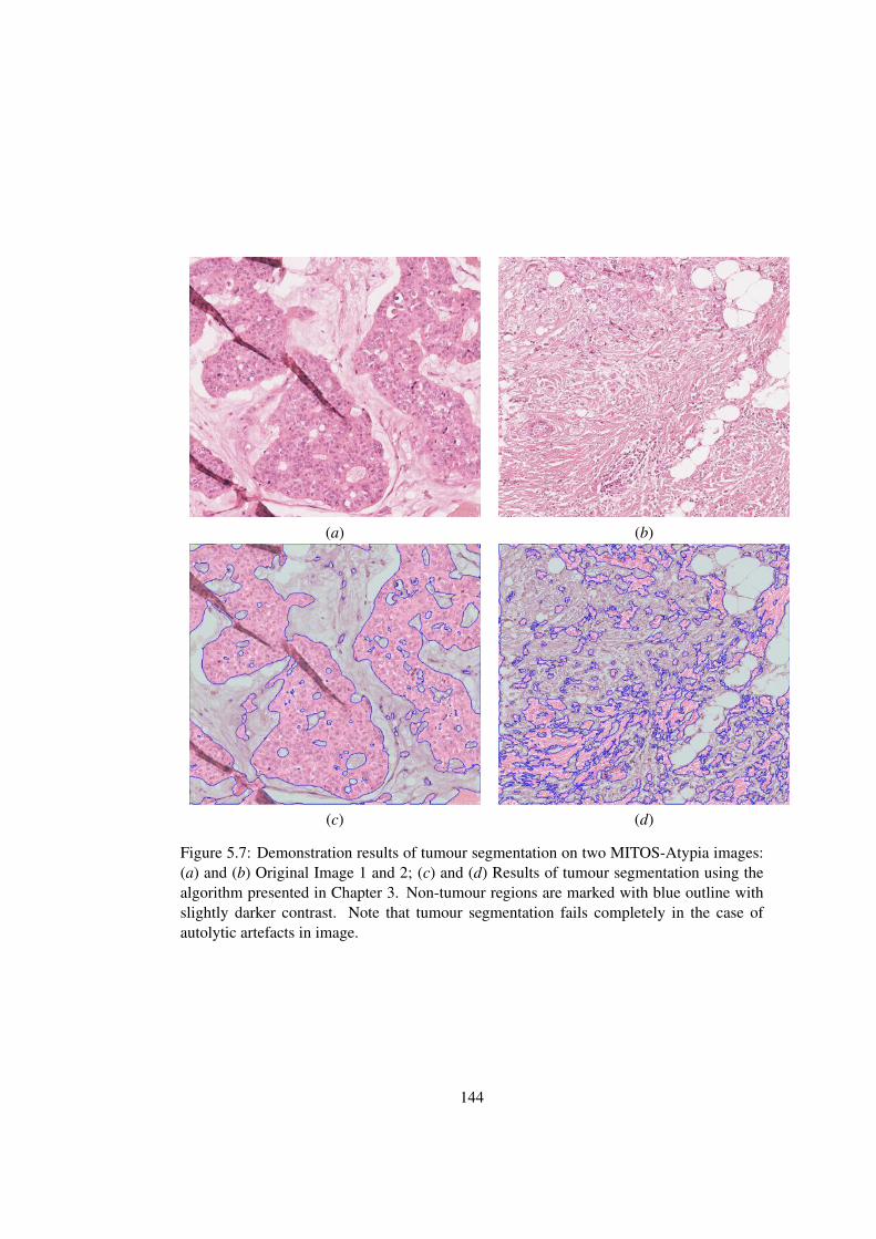
(a) (b)

(c) (d)

Figure 5.7: Demonstration results of tumour segmentation on two MITOS-Atypia images:(a) and (b) Original Image 1 and 2; (c) and (d) Results of tumour segmentation using thealgorithm presented in Chapter 3. Non-tumour regions are marked with blue outline withslightly darker contrast. Note that tumour segmentation fails completely in the case ofautolytic artefacts in image.

144

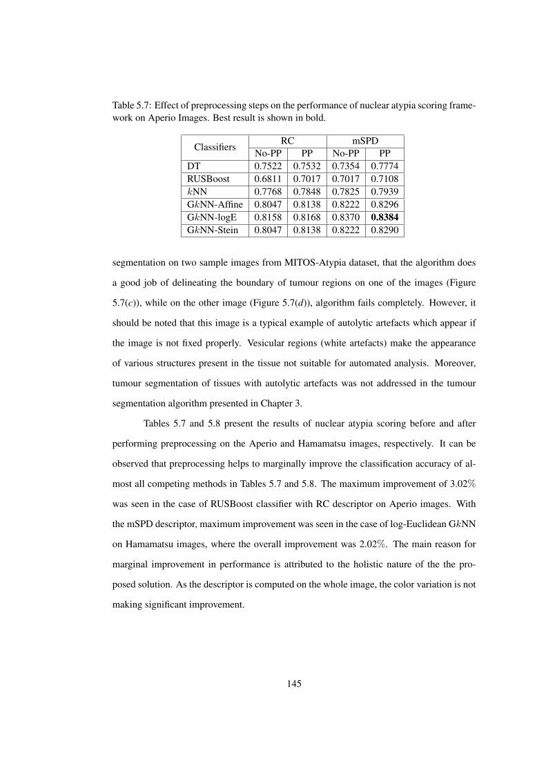
Table 5.7: Effect of preprocessing steps on the performance of nuclear atypia scoring frame-work on Aperio Images. Best result is shown in bold.

ClassifiersRC mSPD

No-PP PP No-PP PPDT 0.7522 0.7532 0.7354 0.7774RUSBoost 0.6811 0.7017 0.7017 0.7108kNN 0.7768 0.7848 0.7825 0.7939GkNN-Affine 0.8047 0.8138 0.8222 0.8296GkNN-logE 0.8158 0.8168 0.8370 0.8384GkNN-Stein 0.8047 0.8138 0.8222 0.8290

segmentation on two sample images from MITOS-Atypia dataset, that the algorithm does

a good job of delineating the boundary of tumour regions on one of the images (Figure

5.7(c)), while on the other image (Figure 5.7(d)), algorithm fails completely. However, it

should be noted that this image is a typical example of autolytic artefacts which appear if

the image is not fixed properly. Vesicular regions (white artefacts) make the appearance

of various structures present in the tissue not suitable for automated analysis. Moreover,

tumour segmentation of tissues with autolytic artefacts was not addressed in the tumour

segmentation algorithm presented in Chapter 3.

Tables 5.7 and 5.8 present the results of nuclear atypia scoring before and after

performing preprocessing on the Aperio and Hamamatsu images, respectively. It can be

observed that preprocessing helps to marginally improve the classification accuracy of al-

most all competing methods in Tables 5.7 and 5.8. The maximum improvement of 3.02%

was seen in the case of RUSBoost classifier with RC descriptor on Aperio images. With

the mSPD descriptor, maximum improvement was seen in the case of log-Euclidean GkNN

on Hamamatsu images, where the overall improvement was 2.02%. The main reason for

marginal improvement in performance is attributed to the holistic nature of the the pro-

posed solution. As the descriptor is computed on the whole image, the color variation is not

making significant improvement.

145

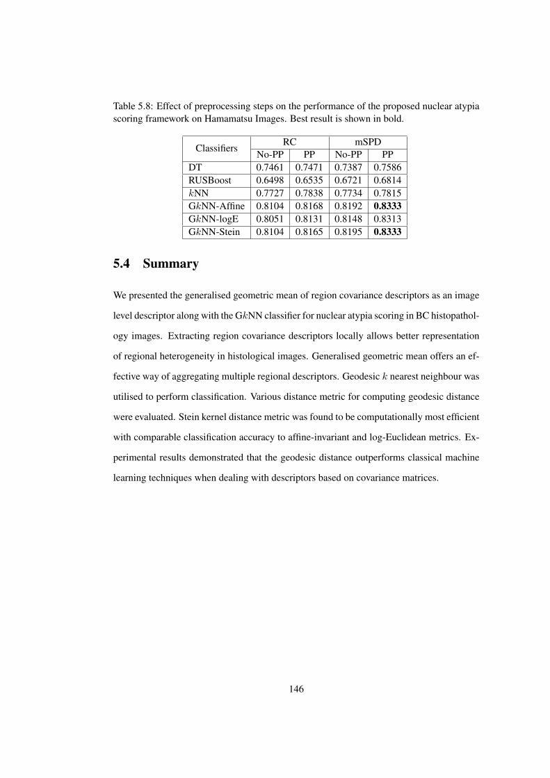
Table 5.8: Effect of preprocessing steps on the performance of the proposed nuclear atypiascoring framework on Hamamatsu Images. Best result is shown in bold.

ClassifiersRC mSPD

No-PP PP No-PP PPDT 0.7461 0.7471 0.7387 0.7586RUSBoost 0.6498 0.6535 0.6721 0.6814kNN 0.7727 0.7838 0.7734 0.7815GkNN-Affine 0.8104 0.8168 0.8192 0.8333GkNN-logE 0.8051 0.8131 0.8148 0.8313GkNN-Stein 0.8104 0.8165 0.8195 0.8333

5.4 Summary

We presented the generalised geometric mean of region covariance descriptors as an image

level descriptor along with the GkNN classifier for nuclear atypia scoring in BC histopathol-

ogy images. Extracting region covariance descriptors locally allows better representation

of regional heterogeneity in histological images. Generalised geometric mean offers an ef-

fective way of aggregating multiple regional descriptors. Geodesic k nearest neighbour was

utilised to perform classification. Various distance metric for computing geodesic distance

were evaluated. Stein kernel distance metric was found to be computationally most efficient

with comparable classification accuracy to affine-invariant and log-Euclidean metrics. Ex-

perimental results demonstrated that the geodesic distance outperforms classical machine

learning techniques when dealing with descriptors based on covariance matrices.

146

Chapter 6

Conclusions and Future Directions

Over the last few years, digital imaging in histopathology has undergone significant growth

mainly because of improvements in imaging hardware and gains in computational pro-

cessing. During the same time, several advancements have been made on the algorithmic

fronts of quantitative histological image analysis as well. Digital pathology is driving the

current histological practices into the digital era by integrating histological image features

with high-dimensional molecular, radiological and genetic features for personalised pa-

tient care. In this thesis, we have presented quantitative image analysis techniques that can

serve as building blocks for digital pathology based cancer grading platforms. This chap-

ter summarises and concludes the work presented in this thesis and discusses some future

directions.

In Chapter 1, we introduced the reader to the standard diagnostic process for BC.

Of various options for BC screening, analysis of tissue under the microscope by an expert

pathologist is still considered as the gold standard throughout the world. We described var-

ious methods for preparing and digitising a histological tissue specimen for microscopic

analysis. We briefly introduced the whole-slide scanners which take a glass slide as input

and generate a multi-gigapixel fully digital WSI as output. For instance, digitising a 1cm2

tissue specimen at 20×magnification produces a histological WSI of size≈ 4GB. In order

to deal with the storage challenges that arise due to the digitisation of histological slides,

148

highly compressible image formats like JPEG2000 are being currently utilised. We further

described the histological grading process of BC using the so-called Nottingham grading

system. The system essentially combines the quantitative scores from three indicators: the

deviation of size and shape of nuclei from the normal epithelial nuclei – nuclear atypia, the

percentage of the tumour that does not form normal duct structures – tubular formation,

and the number of mitotic cells in 10 consecutive high power fields – mitotic index. The

motivation behind this work was to explore the opportunities offered by digital WSIs for

accurate quantification of two out of the three BC grade indicators; mitotic count and nu-

clear atypia to be more specific. A brief description of various datasets used in this work

was also presented. This included a brief description of the WarMiCe dataset that was

collected in collaboration with pathologists at the UHCW for mitotic cell detection in BC

histopathology images.

6.1 Main Contributions

In Chapter 2, we presented an automated algorithm for stain normalisation in histological

images. The algorithm is based on non-linear mapping of the staining characteristics from a

reference image, with ideal staining characteristics, to a target image with non-ideal staining

characteristics. Staining characteristics were estimated by deconvolution of an RGB histo-

logical image into the corresponding stains using Beer-Lambert law [78]. Our contribution

in this context is four fold: (1) We introduced a novel whole-image descriptor (SCD) that

grossly quantifies the concentration of histological stains in an image. We demonstrated

that using SCD along with R, G, B pixel information produce robust pixel classification

of histological images; (2) We proposed the use of a colour based classifier to calculate

image-specific stain matrices, that were shown to be critical to more accurate stain de-

convolution; (3) We performed non-linear mapping of source image channels to the target

image channels using regularised spline based functions estimated from image statistics;

(4) We demonstrated using a real world application that the performance of an automated

149

image analysis algorithm improved significantly when images were stain normalised as a

preprocessing step to the automated analysis. The proposed system was evaluated on two

different datasets from three different tissues (breast, liver and oesophagus), collected at

different times, by different technicians, working at different centres.

In Chapter 3, we presented an algorithm for automatically performing tumour seg-

mentation in BC histopathology images, that were obtained from digitised histological

slides at high magnification (40×). Our contribution in this chapter is two fold: (1) We

addressed the issue of robustness of clustering results in the context of RPs, which demon-

strate significantly different segmentation results due to the very nature of random matrices

that are used to perform low-dimensional embedding of high dimensional feature vectors.

Combining multiple random matrices provides luxury of exploring different parts of the

feature space using random subspace projection. We exploited this idea and developed a

framework for random projections with ensemble clustering. (2) We presented an algorithm

for segmentation of tumour areas in BC histopathology images based on segmentation of

the image into hypo-cellular stroma and hyper-cellular stroma using magnitude and phase

spectra in the Gabor domain. The complimentary nature of the segmentation of the two stro-

mal subtypes was shown, resulting in high segmentation accuracy for the tumour areas.The

proposed system achieved high segmentation accuracy on the MITOS BC histopathology

image dataset. Both stain normalisation and tumour segmentation algorithms are employed

in the subsequent chapters, where we develop algorithm for mitotic cell detection and nu-

clear atypia scoring in BC histopathology images.

In Chapter 4, we presented an algorithm that mimicked a pathologist’s top-down

approach to mitotic cell detection while grading BC slides, i.e. within the tumour regions,

identifying hyperchromatic objects and evaluate each hyperchromatic object for being a

mitotic cell. Our contribution in this chapter is four fold: (1) We proposed GGMM for

detecting mitotic cells in BC histopathology images. Image intensities were modelled as

random variables sampled from one of the two distributions: Gamma and Gaussian. Intensi-

ties from mitotic cells were modelled by a Gamma distribution and those from non-mitotic

150

regions were modelled by a Gaussian distribution; (2) We proposed context, i.e. texture

surrounding a cell, as a clue for classifying cells into mitotic and non-mitotic classes; (3)

We employed cell words, a novel framework for modelling the visual appearance of cells

in histopathology images and applied this model to discriminate between mitotic cells and

non-mitotic cells; (4) We showed that segmentation of tumour regions in BC histopathol-

ogy images plays an important role in improving the performance of mitotic cell detec-

tion framework, leading to more accurate automated BC grading. The proposed system

achieved high detection performance on two BC histopathology image datasets: MITOS

and WarMiCe.

In Chapter 5, we presented a nuclear atypia scoring framework where the gener-

alised geometric mean of region covariance descriptors was used as an image level descrip-

tor to characterise the texture of images associated with different nuclear atypia scores.

We used this novel descriptor in conjunction with the Gk-NN classifier for predicting nu-

clear atypia scores in BC histopathology images. Our contribution in this chapter is four

fold: (1) We presented a novel image descriptor (mSPD) that summarises the texture at-

tributes of an image and demonstrate its usefulness in the context of histological image

analysis application; (2) We exploited GkNN classification approach to assign labels to a

test input image and demonstrate its superiority, as compared to the classical pattern clas-

sification approaches, as it exploits the structure of Riemannian manifold by incorporating

non-Euclidean distance measures; (3) We presented a comparison with a baseline texture

based image classification framework that compute a library of texture features and employ

three classification paradigms to perform nuclear atypia scoring; (4) We presented a range

of experiments that evaluate the performance of the proposed nuclear atypia scoring algo-

rithm in terms of classification accuracy as well as computational time. We also evaluated

performance of the proposed algorithms, when certain preprocessing steps like stain nor-

malisation (Chapter 2) and tumour segmentation (Chapter 3) were incorporated in nuclear

atypia scoring framework.

151

6.2 Future Directions

The tools proposed in this thesis can potentially aid towards building an automated BC

grading system. In the following, we discuss some possible lines of work for extending and

improving the performance of these tools.

SCD has been very successful in increasing the colour consistency. The descriptor

could be used for a wide variety of tasks in histopathology image analysis from segmenta-

tion to similarity-based retrieval, content filtering and visualisation applications. The speed

of stain normalisation algorithm is a concern and can be improved (using e.g. graphics

processing unit (GPU) based implementation). This is important especially considering the

computational demands of a WSI. We demonstrated an application of stain normalisation

in quantitative histological image analysis algorithm. However, we anticipate application

of this technique to a wide range of problems in histopathology image analysis in the near

future.

Tumour segmentation algorithm performed well on large number of histological

images, however the algorithm failed while dealing with images where the tissues were not

fixed properly and had vesicular regions. An easy way to fix this issue would be to develop

an automated method that detects images with vesicular artefacts. That way, one can make

sure not to perform tumour segmentation on images with vesicular artefacts. Alternatively,

one can develop more efficient algorithms that implicitly deal with images having vesicular

artefacts. Ensemble clustering framework can be improved by replacing heuristic based

approach for combining the ensemble clustering results with a more principled approach.

Our possible direction could be the use of region covariance descriptor to calculate the

similarity of a region (either stroma or tumour). Nearest neighbour based classification

framework can be utilised to achieve this goal. Although we demonstrated two applications

of the tumour segmentation algorithm: mitotic cell detection and nuclear atypia scoring, we

anticipate more application of this algorithm in near future.

Many improvements can be made in the proposed mitotic cell detection framework.

152

Currently, detection and classification of the mitotic cell are two separate phases of the al-

gorithm. A potential improvement of the detection framework would be to unify for each

pixel the intensity and contextual information within a single learning framework. More-

over, the framework uses hard thresholding (estimated based on receiver operating charac-

teristic curve) to identify candidate mitotic cells which may result in spurious or erroneous

segmentations of mitotic cells. Some spatial regularisation framework (e.g. Markov ran-

dom field, active contours) could be used to recover such areas. The use of such frameworks

that deal with a probabilistic output could help taking advantage of the level of uncertainty

at each pixel and could provide a softer segmentation than a rough threshold currently does.

However, this may also significantly increase the computational requirements of the frame-

work.

The proposed mitotic cell detection framework can also be adopted to detect other

types of cells (e.g. lymphocytes, immune cells, necrotic cells, etc.) stained with the standard

H&E or IHC stains. Discriminative dictionary learning problem will then become a multi-

class classification problem instead of the binary classification problem presented in this

thesis. However, the objective function of the proposed framework will still remain the

same.

While detecting mitotic cells on a conventional microscope, pathologists have a

privilege to fine tune the focus of the conventional microscope. This feature is missing in

the WSIs captured at a single focal plane by the whole-slide imaging scanners. Although

the present day WSI scanners provide support for multiple focal planes, yet the use of this

feature is still limited because of high storage requirements and increased scanning time.

According to a recent study by Al-Janabi et al. [26], it was concluded that there exists al-

most perfect inter-observer agreement among pathologists’ mitotic score on a conventional

microscope and whole-slide digital images obtained at a single focal plane. Thus, the qual-

ity of histological image obtained by digitising a glass slide is sufficient to perform BC

grading task. Although, digital slides are not still widely accepted as a primary diagnostic

modality, yet such studies provide an indication of more widespread use of digital scanners

153

and automated diagnostic tools based on digital slides in the near future.

The ground truth of all datasets used for mitotic cell detection in this research were

annotated by pathologists, which means all the automated quantitative algorithms are trying

to meet the performance of human experts. A possibly more reliable way of obtaining GT

annotations would be to use specialised stains, e.g. Phosphohistone H3 antibody that has

been shown to be very successful for staining mitotic cells exclusively, and perhaps it will

provide a more reliable GT annotation for mitotic cells [284].

Generalised geometric mean descriptor was shown to be successful as an image

descriptor in Chapter 5. In the near future, we anticipate application of this descriptor to a

wide range of applications that are not limited to histopathology image analysis. Another

possible direction will be to utilise generalised geometric mean image descriptor in sparse

coding and dictionary learning frameworks in order to learn discriminative dictionaries of

textures in a machine learning framework.

154

Bibliography

[1] National Cancer Institute. What is cancer? URL http://www.cancer.

gov/cancertopics/cancerlibrary/what-is-cancer. Accessed: 10-

07-2014.

[2] R Alteri, C Barnes, and A Burke. American cancer society. Breast Cancer Facts &

Figures 2013-2014, 2013.

[3] BreastCancer.org. What Is Breast Cancer? URL http://www.breastcancer.

org/symptoms/understand_bc/what_is_bc. Accessed: 2014-06-14.

[4] Adnan M Khan, Aisha F Mohammed, Shama A Al-Hajri, Hajer M Al Shamari, Uvais

Qidwai, Imaad Mujeeb, and Nasir M Rajpoot. A novel system for scoring of hormone

receptors in breast cancer histopathology slides. In 2nd Middle East Conference on

Biomedical Engineering (MECBME), pages 155–158. IEEE, 2014.

[5] Siemens. Mammography. URL http://www.medicalradiation.

com/types-of-medical-imaging/imaging-using-x-rays/

mammography/. Accessed: 2014-06-14.

[6] The National Breast Cancer Foundation. Ultrasound. URL http://www.

nationalbreastcancer.org/breast-ultrasound. Accessed: 2014-

06-14.

[7] WebMD Medical Reference from Healthwise. Breast cancer health

center. URL http://www.webmd.com/breast-cancer/

stereotactic-biopsy-of-the-breast. Accessed: 2014-06-14.

156

[8] BreastCancer.org. Stages of breast cancer. BreastCancer.org. URL http://www.

breastcancer.org/symptoms/diagnosis/staging. Accessed: 2014-

06-14.

[9] Cancer Research UK. Breast cancer tests. URL http://www.

cancerresearchuk.org/cancer-help/type/breast-cancer/

diagnosis/breast-cancer-tests. Accessed: 10-07-2014.

[10] Geoffrey Rolls. An introduction to specimen preparation. URL

http://www.leicabiosystems.com/pathologyleaders/

an-introduction-to-specimen-preparation/. Accessed: 2014-

06-14.

[11] Antonio C Wolff, M Elizabeth H Hammond, Jared N Schwartz, Karen L Hagerty,

D Craig Allred, Richard J Cote, Mitchell Dowsett, Patrick L Fitzgibbons, Wedad M

Hanna, Amy Langer, Lisa M. McShane, Soonmyung Paik, Mark D. Pegram, Edith A.

Perez, Michael F. Press, Anthony Rhodes, Catharine Sturgeon, Sheila E. Taube, Ray-

mond Tubbs, Gail H. Vance, Marc van de Vijver, Thomas M. Wheeler, and Daniel F.

Hayes. American society of clinical oncology/college of american pathologists

guideline recommendations for human epidermal growth factor receptor 2 testing

in breast cancer. Journal of Clinical Oncology, 25(1):118–145, 2006.

[12] M Elizabeth H Hammond, Daniel F Hayes, Mitch Dowsett, D Craig Allred, Karen L

Hagerty, Sunil Badve, Patrick L Fitzgibbons, Glenn Francis, Neil S Goldstein, Mal-

colm Hayes, David G. Hicks, Susan Lester, Richard Love, Pamela B. Mangu, Lisa

McShane, Keith Miller, Soonmyung Osborne, Kent Paik, Jane Perlmutter, Anthony

Rhodes, Hironobu Sasano, Jared N. Schwartz, Fred C. G. Sweep, Sheila Taube, Em-

ina Emilia Torlakovic, Paul Valenstein, Giuseppe Viale, Daniel Visscher, Thomas

Wheeler, Bruce Williams, James L. Wittliff, and Antonio C. Wolff. American society

of clinical oncology/college of american pathologists guideline recommendations for

immunohistochemical testing of estrogen and progesterone receptors in breast can-

cer (unabridged version). Archives of Pathology & Laboratory Medicine, 134(7):

e48–e72, 2010.

157

[13] Patrick L Fitzgibbons, David L Page, Donald Weaver, Ann D Thor, D Craig Allred,

Gary M Clark, Stephen G Ruby, Frances O’Malley, Jean F Simpson, James L Con-

nolly, Daniel F. Hayes, Stephen B. Edge, Allen Lichter, and Stuart J. Schnitt. Prog-

nostic factors in breast cancer: College of american pathologists consensus statement

1999. Archives of Pathology & Laboratory Medicine, 124(7):966–978, 2000.

[14] RA Walker. Quantification of immunohistochemistryissues concerning methods,

utility and semiquantitative assessment I. Histopathology, 49(4):406–410, 2006.

[15] CR Taylor and RM Levenson. Quantification of immunohistochemistry-issues con-

cerning methods, utility and semiquantitative assessment II. Histopathology, 49(4):

411–424, 2006.

[16] Arthur W Wetzel, R Gilbertson II John, Jeffrey A Beckstead, Patricia A Feineigle,

Christopher R Hauser, and Frank A Palmieri Jr. System for creating microscopic

digital montage images, December 26 2006. US Patent 7,155,049.

[17] Hamamatsu. Digital slide scanner NanoZoomer-XR C12000. URL

http://www.hamamatsu.com/jp/en/product/category/5002/

5007/C12000/index.html. Accessed: 2014-06-14.

[18] 3DHISTECH. 3DHISTECH. URL http://www.3dhistech.com/. Accessed:

2014-06-14.

[19] Omnyx GE. Omnyx GE. URL http://www.omnyx.com/. Accessed: 2014-06-

14.

[20] Ventana. Ventana. URL http://www.ventana.com/product/page?

view=iscan. Accessed: 2014-06-14.

[21] Philips. The Philips digital pathology solution. URL http://www.research.

philips.com/initiatives/digitalpathology/approach.html.

Accessed: 2014-06-14.

[22] Leica BioSystems. Aperio AT2. URL http://www.leicabiosystems.

158

com/pathology-imaging/epathology/scientists/

image-capture-devices/aperior-at2/. Accessed: 2014-06-14.

[23] Marcela Iregui, Francisco Gomez, and Eduardo Romero. Strategies for efficient

virtual microscopy in pathological samples using JPEG2000. Micron, 38(7):700–

713, 2007.

[24] Farzad Ghaznavi, Andrew Evans, Anant Madabhushi, and Michael Feldman. Digital

imaging in pathology: whole-slide imaging and beyond. Annual Review of Pathol-

ogy: Mechanisms of Disease, 8:331–359, 2013.

[25] Christopher W Elston and Ian O Ellis. Pathological prognostic factors in breast

cancer. I. the value of histological grade in breast cancer: experience from a large

study with long-term follow-up. Histopathology, 19(5):403–410, 1991.

[26] Shaimaa Al-Janabi, Henk-Jan van Slooten, Mike Visser, Tjeerd van der Ploeg, Paul J

van Diest, and Mehdi Jiwa. Evaluation of mitotic activity index in breast cancer

using whole slide digital images. PloS One, 8(12):e82576, 2013.

[27] Robert D. Cardiff and Roy A. Jensen. Histological grading of breast

cancer. URL http://ccm.ucdavis.edu/bcancercd/311/grading_

diagram.html. Accessed: 10-07-2014.

[28] Frederic Clayton. Pathologic correlates of survival in 378 lymph node–negative in-

filtrating ductal breast carcinomas. Mitotic count is the best single predictor. Cancer,

68(6):1309–1317, 1991.

[29] Jack Cuzick, Mitch Dowsett, Silvia Pineda, Christopher Wale, Janine Salter, Emma

Quinn, Lila Zabaglo, Elizabeth Mallon, Andrew R Green, Ian O Ellis, Anthony How-

ell, Aman U. Buzdar, and John F. Forbes. Prognostic value of a combined estrogen

receptor, progesterone receptor, Ki-67, and human epidermal growth factor receptor

2 immunohistochemical score and comparison with the genomic health recurrence

score in early breast cancer. Journal of Clinical Oncology, 29(32):4273–4278, 2011.

159

[30] Yinyin Yuan, Henrik Failmezger, Oscar M Rueda, H Raza Ali, Stefan Graf, Suet-

Feung Chin, Roland F Schwarz, Christina Curtis, Mark J Dunning, Nicola Bardwell,

Helen Johnson, Sarah Doyle, Gulisa Turashvili, Elena Provenzano, Sam Aparicio,

Carlos Caldas, and Florian Markowetz. Quantitative image analysis of cellular het-

erogeneity in breast tumors complements genomic profiling. Science Translational

Medicine, 4(157):157ra143–157ra143, 2012.

[31] Statistical Information Team. Breast cancer. Key facts, Cancer Research, UK, 2014.

[32] Stuart J Schnitt, James L Connolly, Fattaneh A Tavassoli, Robert E Fechner,

Richard L Kempson, Rebecca Gelman, and David L Page. Interobserver repro-

ducibility in the diagnosis of ductal proliferative breast lesions using standardized

criteria. The American Journal of Surgical Pathology, 16(12):1133–1143, 1992.

[33] Andreas Stang, Pietro Trocchi, Kathrin Ruschke, Andrea Schmidt-Pokrzywniak,

Hans-Jurgen Holzhausen, Thomas Loning, Jorg Buchmann, Christoph Thomssen,

Tillmann Lantzsch, Steffen Hauptmann, and Alexander Kluttig. Factors influencing

the agreement on histopathological assessments of breast biopsies among patholo-

gists. Histopathology, 59(5):939–949, 2011.

[34] Anant Madabhushi. Digital pathology image analysis: opportunities and challenges.

Imaging in Medicine, 1(1):7–10, 2009.

[35] Andrew H Beck, Ankur R Sangoi, Samuel Leung, Robert J Marinelli, Torsten O

Nielsen, Marc J van de Vijver, Robert B West, Matt van de Rijn, and Daphne Koller.

Systematic analysis of breast cancer morphology uncovers stromal features asso-

ciated with survival. Science Translational Medicine, 3(108):108ra113–108ra113,

2011.

[36] Quoc V Le. Building high-level features using large scale unsupervised learn-

ing. In IEEE International Conference on Acoustics, Speech and Signal Processing

(ICASSP), pages 8595–8598. IEEE, 2013.

[37] Adnan M Khan, Hesham ElDaly, and Rajpoot Nasir M. A Gamma-Gaussian mixture

160

model for detection of mitotic cells in breast cancer histopathology images. Journal

of Pathology Informatics (JPI), 4(11), 2013.

[38] Korsuk Sirinukunwattana, Adnan Mujahid Khan, and Nasir Rajpoot. Cell Words:

Modelling the visual appearance of cells in histopathology images. Computerized

Medical Imaging and Graphics, 2014.

[39] Oncel Tuzel, Fatih Porikli, and Peter Meer. Region covariance: A fast descriptor for

detection and classification. In European Conference on Computer Vision (ECCV),

pages 589–600. Springer, 2006.

[40] Xavier Pennec, Pierre Fillard, and Nicholas Ayache. A Riemannian framework for

tensor computing. International Journal of Computer Vision (IJCV), 66(1):41–66,

2006.

[41] Ludovic Roux, Daniel Racoceanu, Nicolas Lomenie, Maria Kulikova, Humayun Ir-

shad, Jacques Klossa, Frederique Capron, Catherine Genestie, Gilles Le Naour, and

Metin Gurcan. Mitosis detection in breast cancer histological images. Journal of

Pathology Informatics (JPI), 4(8):2–8, 2013.

[42] Hans O Lyon, AP De Leenheer, RW Horobin, WE Lambert, EKW Schulte,

B Van Liedekerke, and DH Wittekind. Standardization of reagents and methods

used in cytological and histological practice with emphasis on dyes, stains and chro-

mogenic reagents. The Histochemical Journal, 26(7):533–544, 1994.

[43] Graham D. Finlayson, Steven D. Hordley, and Paul M. Hubel. Color by correlation:

A simple, unifying framework for color constancy. IEEE Transactions on Pattern

Analysis and Machine Intelligence (TPAMI), 23(11):1209–1221, 2001.

[44] Peter W Hamilton, Peter H Bartels, Deborah Thompson, Neil H Anderson, Rodolfo

Montironi, and James M Sloan. Automated location of dysplastic fields in colorectal

histology using image texture analysis. The Journal of Pathology, 182(1):68–75,

1997.

161

[45] Matthew D DiFranco, Gillian OHurley, Elaine W Kay, R William G Watson, and

Padraig Cunningham. Ensemble based system for whole-slide prostate cancer prob-

ability mapping using color texture features. Computerized Medical Imaging and

Graphics (CMIG), 35(7):629–645, 2011.

[46] Antonio Ruiz, Olcay Sertel, Manuel Ujaldon, Umit Catalyurek, Joel Saltz, and Metin

Gurcan. Stroma classification for neuroblastoma on graphics processors. Interna-

tional Journal of Data Mining and Bioinformatics, 3(3):280–298, 2009.

[47] Timo Ojala, Matti Pietikainen, and Topi Maenpaa. Multiresolution gray-scale and

rotation invariant texture classification with local binary patterns. IEEE Transactions

on Pattern Analysis and Machine Intelligence (TPAMI), 24(7):971–987, 2002.

[48] Hammad Qureshi, Olcay Sertel, Nasir Rajpoot, Roland Wilson, and Metin Gurcan.

Adaptive discriminant wavelet packet transform and local binary patterns for menin-

gioma subtype classification. In Medical Image Computing and Computer-Assisted

Intervention (MICCAI), pages 196–204. Springer, 2008.

[49] Ajay Nagesh Basavanhally, Shridar Ganesan, Shannon Agner, James Peter Monaco,

Michael D Feldman, John E Tomaszewski, Gyan Bhanot, and Anant Madabhushi.

Computerized image-based detection and grading of lymphocytic infiltration in

HER2+ breast cancer histopathology. IEEE Transactions on Biomedical Engineering

(TBME), 57(3):642–653, 2010.

[50] Andrew Janowczyk, Sharat Chandran, Rajendra Singh, Dimitra Sasaroli, George

Coukos, Michael D Feldman, and Anant Madabhushi. High-throughput biomarker

segmentation on ovarian cancer tissue microarrays via hierarchical normalized cuts.

IEEE Transactions on Biomedical Engineering (TBME), 59(5):1240–1252, 2012.

[51] Jason D Hipp, Jerome Y Cheng, Mehmet Toner, Ronald G Tompkins, and Ulysses J.

Balis. Spatially invariant vector quantization: A pattern matching algorithm for mul-

tiple classes of image subject matter including pathology. Journal of Pathology In-

formatics (JPI), 2(1):13, 2011.

162

[52] Jun Kong, Olcay Sertel, Hiroyuki Shimada, Kim Boyer, Joel Saltz, and Metin Gur-

can. Computer-aided grading of neuroblastic differentiation: Multi-resolution and

multi-classifier approach. In International Conference on Image Processing (ICIP),

volume 5, pages 525–528. IEEE, 2007.

[53] Olcay Sertel, Jun Kong, Hiroyuki Shimada, Umit Catalyurek, Joel H Saltz, and Metin

Gurcan. Computer-aided prognosis of neuroblastoma: classification of stromal de-

velopment on whole-slide images. In SPIE Medical Imaaging. Society of Photo-

Optical Instrumentation Engineers, 2008.

[54] James Monaco, J Hipp, D Lucas, S Smith, U Balis, and Anant Madabhushi. Im-

age segmentation with implicit color standardization using spatially constrained Ex-

pectation Maximization: Detection of nuclei. In Medical Image Computing and

Computer-Assisted Intervention (MICCAI), pages 365–372. Springer, 2012.

[55] James Monaco, Philipp Raess, Ronak Chawla, Adam Bagg, Mitchell Weiss, John

Choi, and Anant Madabhushi. Image segmentation with implicit color standardiza-

tion using cascaded EM: detection of myelodysplastic syndromes. In 9th IEEE In-

ternational Symposium on Biomedical Imaging (ISBI), pages 740–743. IEEE, 2012.

[56] Sonal Kothari, John H Phan, Richard A Moffitt, Todd H Stokes, Shelby E Hassberger,

Qaiser Chaudry, Andrew N Young, and May D Wang. Automatic batch-invariant

color segmentation of histological cancer images. In IEEE International Symposium

on Biomedical Imaging: From Nano to Macro (ISBI), pages 657–660. IEEE, 2011.

[57] Erik Reinhard, Michael Ashikhmin, Bruce Gooch, and Peter Shirley. Color transfer

between images. IEEE Computer Graphics and Applications, 21(5):34–41, 2001.

[58] Derek Magee, Darren Treanor, Doreen Crellin, Mike Shires, Katherine Smith, Kevin

Mohee, and Philip Quirke. Colour normalisation in digital histopathology images. In

Optical Tissue Image Analysis in Microscopy, Histopathology and Endoscopy (MIC-

CAI Workshop), pages 20–24, 2009.

[59] Marc Macenko, Marc Niethammer, JS Marron, David Borland, John T Woosley,

Xiaojun Guan, Charles Schmitt, and Nancy E Thomas. A method for normaliz-

163

ing histology slides for quantitative analysis. In IEEE International Symposium on

Biomedical Imaging : From Nano to Macro (ISBI), pages 1107–1110. IEEE, 2009.

[60] Marc Niethammer, David Borland, JS Marron, John Woosley, and Nancy E Thomas.

Appearance normalization of histology slides. In Machine Learning in Medical

Imaging (MLMI), pages 58–66. Springer, 2010.

[61] Cemal Cagatay Bilgin, Jens Rittscher, R Filkins, and Ali Can. Digitally adjust-

ing chromogenic dye proportions in brightfield microscopy images. Journal of Mi-

croscopy, 245(3):319–330, 2012.

[62] Ajay Basavanhally and Anant Madabhushi. EM-based segmentation-driven color

standardization of digitized histopathology. In SPIE Medical Imaging. International

Society for Optics and Photonics, 2013.

[63] Pinky A Bautista, Noriaki Hashimoto, and Yukako Yagi. Color standardization in

whole slide imaging using a color calibration slide. Journal of Pathology Informatics

(JPI), 5, 2014.

[64] Adnan M Khan, Nasir Rajpoot, Darren Treanor, and Derek Magee. A non-linear

mapping approach to stain normalisation in digital histopathology images using

image-specific colour deconvolution. IEEE Transactions on Biomedical Engineering

(TBME), 61(6):1729–1738, 2014.

[65] Yi-Ying Wang, Shao-Chien Chang, Li-Wha Wu, Sen-Tien Tsai, and Yung-Nien Sun.

A color-based approach for automated segmentation in tumor tissue classification. In

International Conference of the IEEE Engineering in Medicine and Biology Society

(EMBC), pages 6576–6579. IEEE, 2007.

[66] Anil K Jain. Fundamentals of Digital Image Processing. Prentice-Hall, 1989.

[67] Yukako Yagi. Color standardization and optimization in whole slide imaging. Diag-

nostic Pathology, 6(Suppl 1):S15, 2011.

[68] Shinsuke Tani, Yasuhiro Fukunaga, Saori Shimizu, Munenori Fukunishi, Kensuke

Ishii, and Kosei Tamiya. Color standardization method and system for whole slide

164

imaging based on spectral sensing. Analytical Cellular Pathology, 35(2):107–115,

2012.

[69] Yuri Murakami, Hikaru Gunji, Fumikazu Kimura, Masahiro Yamaguchi, Yoshiko

Yamashita, Akira Saito, Tokiya Abe, Michiie Sakamoto, Pinky A Bautista, and

Yukako Yagi. Color correction in whole slide digital pathology. In Color and

Imaging Conference, volume 2012, pages 253–258. Society for Imaging Science

and Technology, 2012.

[70] Yuri Murakami, Tokiya Abe, Akinori Hashiguchi, Masahiro Yamaguchi, Akira Saito,

and Michiie Sakamoto. Color correction for automatic fibrosis quantification in liver

biopsy specimens. Journal of Pathology Informatics (JPI), 4, 2013.

[71] M Muthu Rama Krishnan, Pratik Shah, Chandan Chakraborty, and Ajoy K Ray.

Statistical analysis of textural features for improved classification of oral histopatho-

logical images. Journal of Medical Systems (JMS), 36(2):865–881, 2012.

[72] Alireza Osareh, Majid Mirmehdi, Bari Thomas, and Richard Markham. Automated

identification of diabetic retinal exudates in digital colour images. British Journal of

Ophthalmology, 87(10):1220–1223, 2003.

[73] Arnout C Ruifrok and Dennis A Johnston. Quantification of histochemical staining

by color deconvolution. Analytical and Quantitative Cytology and Histology/the

International Academy of Cytology & American Society of Cytology, 23(4):291–299,

2001.

[74] Milan Gavrilovic, Jimmy C Azar, Joakim Lindblad, Carolina Wahlby, Ewert Bengts-

son, Christer Busch, and Ingrid B Carlbom. Blind color decomposition of histologi-

cal images. IEEE Transactions on Medical Imaging (TMI), 32(6):983–994, 2013.

[75] Adnan M Khan, Hesham El-Daly, and Nasir Rajpoot. RanPEC: Random Projections

with Ensemble Clustering for Segmentation of Tumor Areas in Breast Histology Im-

ages. In Medical Image Understanding and Analysis (MIUA), pages 17–23. British

Machine Vision Association (BMVA), 2012.

165

[76] Derek Magee, Darren Treanor, P Chomphuwiset, and P Quirke. Context aware

colour classification in digital microscopy. In Medical Image Understanding and

Analysis (MIUA), pages 1–5. British Machine Vision Association (BMVA), 2010.

[77] Manohar Kuse, Yi-Fang Wang, Vinay Kalasannavar, Michael Khan, and Nasir Ra-

jpoot. Local isotropic phase symmetry measure for detection of beta cells and lym-

phocytes. Journal of Pathology Informatics (JPI), 2, 2011.

[78] William W Parson. Modern Optical Spectroscopy. Springer, 2007.

[79] Michael Gervautz and Werner Purgathofer. A simple method for color quantization:

Octree quantization. In New Trends in Computer Graphics, pages 219–231. Springer,

1988.

[80] Gabriella Csurka, Christopher Dance, Lixin Fan, Jutta Willamowski, and Cedric

Bray. Visual categorization with bags of keypoints. In ECCV Workshop on Sta-

tistical Learning in Computer Vision, volume 1, pages 1–2, 2004.

[81] Michael E Tipping. Sparse Bayesian learning and the relevance vector machine.

Journal of Machine Learning Research (JMLR), 1:211–244, 2001.

[82] Michael E Tipping and Anita C Faul. Fast marginal likelihood maximisation for

sparse bayesian models. In 9th International Workshop on Artificial Intelligence and

Statistics, 2003.

[83] Corinna Cortes and Vladimir Vapnik. Support-vector networks. Machine Learning,

20(3):273–297, 1995.

[84] Leo Breiman. Random forests. Machine Learning, 45(1):5–32, 2001.

[85] Vladimir Svetnik, Andy Liaw, Christopher Tong, J Christopher Culberson, Robert P

Sheridan, and Bradley P Feuston. Random forest: a classification and regression tool

for compound classification and QSAR modeling. Journal of Chemical Information

and Computer Sciences (JCICS), 43(6):1947–1958, 2003.

166

[86] Jonathan Milgram, Mohamed Cheriet, and Robert Sabourin. ”One Against One” or

One Against All: Which one is better for handwriting recognition with SVMs? In

10th International Workshop on Frontiers in Handwriting Recognition, 2006.

[87] Chih-Wei Hsu and Chih-Jen Lin. A comparison of methods for multiclass support

vector machines. IEEE Transactions on Neural Networks (TNN), 13(2):415–425,

2002.

[88] Per Christian Hansen. Rank-deficient and discrete ill-posed problems: numerical

aspects of linear inversion, volume 4. SIAM, 1998. ISBN 0-89871-403-6.

[89] Adnan M Khan, Hesham El-Daly, Emma Simmons, and Nasir M Rajpoot. HyMaP:

A hybrid magnitude-phase approach to unsupervised segmentation of tumor areas in

breast cancer histology images. Journal of Pathology Informatics (JPI), 4(2), 2013.

[90] Hye-Jin Jeong, Tae-Yoon Kim, Hae-Gil Hwang, Hyun-Ju Choi, Hyung-Seon Park,

and Heung-Kook Choi. Comparison of thresholding methods for breast tumor cell

segmentation. In 7th International Workshop on Enterprise Networking and Com-

puting in Healthcare Industry (HEALTHCOM), pages 392–395. IEEE, 2005.

[91] Jean-Romain Dalle, Wee Kheng Leow, Daniel Racoceanu, Adina Eunice Tutac, and

Thomas C Putti. Automatic breast cancer grading of histopathological images. In

30th Annual International Conference of the IEEE Engineering in Medicine and Bi-

ology Society (EMBC), pages 3052–3055. IEEE, 2008.

[92] Andrei Chekkoury, Parmeshwar Khurd, Jie Ni, Claus Bahlmann, Ali Kamen, Amar

Patel, Leo Grady, Maneesh Singh, Martin Groher, and Nassir Navab. Automated

malignancy detection in breast histopathological images. In SPIE Medical Imaging,

volume 8315. International Society for Optics and Photonics, 2012.

[93] Ching-Wei Wang. Robust automated tumour segmentation on histological and im-

munohistochemical tissue images. PloS One, 6(2):e15818, 2011.

[94] Shazia Akbar, Telmo Amaral, Stephen J McKenna, Alastair Thompson, and Lee Jor-

dan. Tumour segmentation in breast tissue microarray images using spin-context. In

167

Medical Image Understanding and Analysis (MIUA), pages 25–30. British Machine

Vision Association (BMVA), 2012.

[95] Shazia Akbar, Stephen J McKenna, Telmo Amaral, Lee Jordan, and Alastair Thomp-

son. Spin-context segmentation of breast tissue microarray images. Annals of the

BMVA, (4):1–11, 2013.

[96] Stephen J McKenna, Telmo Amaral, Shazia Akbar, Lee Jordan, and Alastair Thomp-

son. Immunohistochemical analysis of breast tissue microarray images using con-

textual classifiers. Journal of Pathology Informatics (JPI), 4(Suppl), 2013.

[97] Nina Linder, Juho Konsti, Riku Turkki, Esa Rahtu, Mikael Lundin, Stig Nordling,

Caj Haglund, Timo Ahonen, Matti Pietikainen, and Johan Lundin. Identification of

tumor epithelium and stroma in tissue microarrays using texture analysis. Diagnostic

Pathology, 7:22, 2012.

[98] Claus Bahlmann, Amar Patel, Jeffrey Johnson, Jie Ni, Andrei Chekkoury, Parmesh-

war Khurd, Ali Kamen, Leo Grady, Elizabeth Krupinski, Anna Graham, and Ronald

Weinstein. Automated detection of diagnostically relevant regions in H&E stained

digital pathology slides. In SPIE Medical Imaging, pages 831504–831504. Interna-

tional Society for Optics and Photonics, 2012.

[99] Yan Xu, Jianwen Zhang, I Eric, Chao Chang, Maode Lai, and Zhuowen Tu. Context-

constrained multiple instance learning for histopathology image segmentation. In

Medical Image Computing and Computer-Assisted Intervention (MICCAI), pages

623–630. Springer, 2012.

[100] Yan Xu, Jun-Yan Zhu, Eric I Chang, Maode Lai, and Zhuowen Tu. Weakly super-

vised histopathology cancer image segmentation and classification. Medical Image

Analysis, 18(3):591–604, 2014.

[101] Zoltan Kato, Josiane Zerubia, and Mark Berthod. Satellite image classification using

a modified metropolis dynamics. In IEEE International Conference on Acoustics,

Speech, and Signal Processing (ICASSP), volume 3, pages 573–576. IEEE, 1992.

168

[102] Svetlana Lazebnik, Cordelia Schmid, and Jean Ponce. A sparse texture representa-

tion using local affine regions. IEEE Transactions on Pattern Analysis and Machine

Intelligence (TPAMI), 27(8):1265–1278, 2005.

[103] Zhuowen Tu. Auto-context and its application to high-level vision tasks. In IEEE

Conference on Computer Vision and Pattern Recognition (CVPR), pages 1–8. IEEE,

2008.

[104] Zhuowen Tu and Xiang Bai. Auto-context and its application to high-level vision

tasks and 3d brain image segmentation. IEEE Transactions on Pattern Analysis and

Machine Intelligence (TPAMI), 32(10):1744–1757, 2010.

[105] Zhu Xiaojin. Semi-supervised learning literature survey. Computer Sciences TR,

1530, 2008.

[106] Cha Zhang, John C Platt, and Paul A Viola. Multiple instance boosting for object

detection. In Advances in Neural Information Processing Systems, pages 1417–1424,

2005.

[107] Boris Babenko, Piotr Dollar, Zhuowen Tu, and Serge Belongie. Simultaneous learn-

ing and alignment: Multi-instance and multi-pose learning. In Workshop on Faces in

‘Real-Life’ Images: Detection, Alignment, and Recognition, 2008.

[108] Thomas G Dietterich, Richard H Lathrop, and Tomas Lozano-Perez. Solving the

multiple instance problem with axis-parallel rectangles. Artificial Intelligence, 89

(1):31–71, 1997.

[109] Qingshan Liu, Zhen Qian, Idean Marvasty, Sarah Rinehart, Szilard Voros, and Dim-

itris N Metaxas. Lesion-specific coronary artery calcium quantification for pre-

dicting cardiac event with multiple instance support vector machines. In Medical

Image Computing and Computer-Assisted Intervention (MICCAI), pages 484–492.

Springer, 2010.

[110] Glenn Fung, Murat Dundar, Balaji Krishnapuram, and R Bharat Rao. Multiple in-

169

stance learning for computer aided diagnosis. Advances in Neural Information Pro-

cessing Systems (NIPS), 19:425, 2007.

[111] Roman Sandler and Michael Lindenbaum. Gabor filter analysis for texture segmen-

tation. In Computer Vision and Pattern Recognition Workshop (CVPRW), pages 178–

178. IEEE, 2006.

[112] Jainguo Zhang, Tieniu Tan, and Li Ma. Invariant texture segmentation via circu-

lar Gabor filters. In 16th International Conference on Pattern Recognition (ICPR),

volume 2, pages 901–904. IEEE, 2002.

[113] Simona E Grigorescu, Nicolai Petkov, and Peter Kruizinga. Comparison of texture

features based on Gabor filters. IEEE Transactions on Image Processing (TIP), 11

(10):1160–1167, 2002.

[114] Satish Viswanath and Anant Madabhushi. Consensus embedding: theory, algorithms

and application to segmentation and classification of biomedical data. BMC Bioin-

formatics, 13(1):26, 2012.

[115] Shuicheng Yan, Dong Xu, Benyu Zhang, Hong-Jiang Zhang, Qiang Yang, and

Stephen Lin. Graph embedding and extensions: a general framework for dimension-

ality reduction. IEEE Transactions on Pattern Analysis and Machine Intelligence

(TPAMI), 29(1):40–51, 2007.

[116] Hanchuan Peng, Fulmi Long, and Chris Ding. Feature selection based on mutual

information criteria of max-dependency, max-relevance, and min-redundancy. IEEE

Transactions on Pattern Analysis and Machine Intelligence (TPAMI), 27(8):1226–

1238, 2005.

[117] Harvey B Mitchell. Multi-Sensor Data Fusion. Springer, 2007.

[118] Matteo Bregonzio, Shaogang Gong, and Tao Xiang. Recognising action as clouds

of space-time interest points. In IEEE Conference on Computer Vision and Pattern

Recognition (CVPR), pages 1948–1955. IEEE, 2009.

170

[119] Zhisong He, Jian Zhang, Xiao-He Shi, Le-Le Hu, Xiangyin Kong, Yu-Dong Cai, and

Kuo-Chen Chou. Predicting drug-target interaction networks based on functional

groups and biological features. PloS One, 5(3):e9603, 2010.

[120] Mahesh Pal and Giles M Foody. Feature selection for classification of hyperspectral

data by SVM. IEEE Transactions on Geoscience and Remote Sensing (TGRS), 48

(5):2297–2307, 2010.

[121] Ian Naismith Sneddon. Fourier Transforms. Courier Dover Publications, 1995.

[122] D Gibson and PA Gaydecki. Definition and application of a Fourier domain texture

measure: Applications to histological image segmentation. Computers in Biology

and Medicine (CBM), 25(6):551–557, 1995.

[123] Kamel Belkacem-Boussaid, Olcay Sertel, Gerard Lozanski, Arwa Shana’aah, and

Metin Gurcan. Extraction of color features in the spectral domain to recognize cen-

troblasts in histopathology. In International Conference of the IEEE Engineering in

Medicine and Biology Society (EMBC), pages 3685–3688. IEEE, 2009.

[124] Hui Kong, Metin Gurcan, and Kamel Belkacem-Boussaid. Partitioning histopatho-

logical images: an integrated framework for supervised color-texture segmentation

and cell splitting. IEEE Transactions on Medical Imaging (TMI), 30(9):1661–1677,

2011.

[125] John G Daugman. Uncertainty relation for resolution in space, spatial frequency,

and orientation optimized by two-dimensional visual cortical filters. Journal of the

Optical Society of America A (JOSA A), 2:1160–1169, 1985.

[126] Kashif Murtaza, Sohaib Khan, and Nasir Rajpoot. Villagefinder: Segmentation

of nucleated villages in satellite imagery. In British Mission Vision Conference

(BMVC), pages 1–11. British Machine Vision Association (BMVA), 2009.

[127] Roland Wilson and Michael Spann. Image Segmentation and Uncertainty. John

Wiley & Sons, Inc, 1988.

171

[128] Nasir Rajpoot. Texture classification using discriminant wavelet packet subbands.

In 45th Midwest Symposium on Circuits and Systems (MWSCAS), volume 3, pages

300–303. IEEE, 2002.

[129] Anil K Jain and Farshid Farrokhnia. Unsupervised texture segmentation using Gabor

filters. Pattern Recognition, 24(12):1167–1186, 1991.

[130] Trygve Randen and John Hakon Husoy. Filtering for texture classification: A com-

parative study. IEEE Transactions on Pattern Analysis and Machine Intelligence

(TPAMI), 21(4):291–310, 1999.

[131] Yanwei Pang, Yuan Yuan, and Xuelong Li. Gabor-based region covariance matrices

for face recognition. IEEE Transactions on Circuits and Systems for Video Technol-

ogy, 18(7):989–993, 2008.

[132] HF Qin, L Qin, L Xue, and CB Yu. Gabor-based weighted region covariance matrix

for face recognition. Electronics Letters, 48(16):992–993, 2012.

[133] Itzhak Fogel and Dov Sagi. Gabor filters as texture discriminator. Biological Cyber-

netics, 61(2):103–113, 1989.

[134] Thomas P Weldon, William E Higgins, and Dennis F Dunn. Efficient Gabor filter

design for texture segmentation. Pattern Recognition, 29(12):2005–2015, 1996.

[135] Todd R Reed and JM Hans Dubuf. A review of recent texture segmentation and

feature extraction techniques. CVGIP: Image Understanding, 57(3):359–372, 1993.

[136] David J Field. Relations between the statistics of natural images and the response

properties of cortical cells. Journal of the Optical Society of America (JOSA A), 4

(12):2379–2394, 1987.

[137] S Marcelja. Mathematical description of the responses of simple cortical cells*.

Journal of the Optical Society of America (JOSA), 70(11):1297–1300, 1980.

[138] Hans Du Buf and P. Heitkamper. Texture features based on Gabor phase. Signal

Processing, 23(3):227–244, 1991.

172

[139] Peter Kovesi. Invariant measures of image features from phase information. PhD

thesis, University of Western Australia, 1996.

[140] Nasir Rajpoot and RR Coifman. Phase gradients for texture analysis. In MVA-AVA

Symposium on Image Features and Statistics. MVA-AVA, 2004.

[141] Hans Knutsson. Filtering and reconstruction in image processing. PhD thesis,

Linkoping University, 1982.

[142] Constantino Carlos Reyes Aldasoro and Abhir Bhalerao. Volumetric texture seg-

mentation by discriminant feature selection and multiresolution classification. IEEE

Transactions on Medical Imaging (TMI), 26(1):1–14, 2007.

[143] Constantino Carlos Reyes Aldasoro and Abhir Bhalerao. The Bhattacharyya space

for feature selection and its application to texture segmentation. Pattern Recognition,

39(5):812–826, 2006.

[144] Roland Wilson and AH Bhalerao. Kernel designs for efficient multiresolution edge

detection and orientation estimation. IEEE Transactions on Pattern Analysis and

Machine Intelligence (TPAMI), 14(3):384–390, 1992.

[145] Chang-Tsun Li. Unsupervised texture segmentation using multiresolution Markov

random fields. PhD thesis, University of Warwick, 1998.

[146] P Scheunders, S Livens, G Van de Wouwer, P Vautrot, and D Van Dyck. Wavelet-

based texture analysis. International Journal on Computer Science and Information

Management, 1(2):22–34, 1998.

[147] Ronald R Coifman and M Victor Wickerhauser. Entropy-based algorithms for best

basis selection. IEEE Transactions on Information Theory, 38(2):713–718, 1992.

[148] Mehmet V Tazebay and Ali N Akansu. Adaptive subband transforms in time-

frequency excisers for DSSS communications systems. IEEE Transactions on Signal

Processing (TSP), 43(11):2776–2782, 1995.

[149] Solomon Kullback and Richard A Leibler. On information and sufficiency. The

Annals of Mathematical Statistics, pages 79–86, 1951.

173

[150] William B Johnson and Joram Lindenstrauss. Extensions of lipschitz mappings into

a hilbert space. Contemporary Mathematics, 26(189-206):1–1, 1984.

[151] Sanjoy Dasgupta and Anupam Gupta. An elementary proof of a theorem of Johnson

and Lindenstrauss. Random Structures & Algorithms, 22(1):60–65, 2003.

[152] Sanjoy Dasgupta. Experiments with random projection. In 16th Conference on

Uncertainty in Artificial Intelligence (UAI), pages 143–151. Morgan Kaufmann Pub-

lishers Inc, 2000.

[153] Emmanuel J Candes and Terence Tao. Decoding by linear programming. IEEE

Transactions on Information Theory (TIT), 51(12):4203–4215, 2005.

[154] Emmanuel J Candes and Terence Tao. Near-optimal signal recovery from random

projections: Universal encoding strategies? IEEE Transactions on Information The-

ory (TIT), 52(12):5406–5425, 2006.

[155] David L Donoho. Compressed sensing. IEEE Transactions on Information Theory

(TIT), 52(4):1289–1306, 2006.

[156] David Pollard. Quantization and the method of k-means. IEEE Transactions on

Information theory (TIT), 28(2):199–204, 1982.

[157] Li Liu and Paul W Fieguth. Texture classification from random features. IEEE

Transactions on Pattern Analysis and Machine Intelligence (TPAMI), 34(3):574–

586, 2012.

[158] E. Bingham and H. Mannila. Random projection in dimensionality reduction: appli-

cations to image and text data. In 7th ACM International Conference on Knowledge

Discovery and Data Mining (SIGKDD), pages 245–250. ACM, 2001.

[159] Xiaoli Zhang Fern and Carla E Brodley. Random projection for high dimensional

data clustering: A cluster ensemble approach. In International Conference on Ma-

chine Learning (ICML), volume 20, page 186, 2003.

174

[160] Hanxi Li, Chunhua Shen, and Qinfeng Shi. Real-time visual tracking using com-

pressive sensing. In IEEE Conference on Computer Vision and Pattern Recognition

(CVPR), pages 1305–1312. IEEE, 2011.

[161] Jitendra Malik and Pietro Perona. Preattentive texture discrimination with early vi-

sion mechanisms. Journal of the Optical Society of America A (JOSA A), 7(5):923–

932, 1990.

[162] R.S. Hunter. Photoelectric color difference meter. Journal of Optical Society of

America (JOSA), 48(12):985–993, 1958.

[163] Richard Sewall Hunter. Accuracy, precision, and stability of new photoelectric color-

difference meter. 38(12):1094–1094, 1948.

[164] John A Hartigan and Manchek A Wong. A k-means clustering algorithm. Applied

Statistics, pages 100–108, 1979.

[165] Laurens JP van der Maaten, Eric O Postma, and H Jaap van den Herik. Dimen-

sionality reduction: A comparative review. Journal of Machine Learning Research

(JMLR), 10(1-41):66–71, 2009.

[166] Michael W Schwarz, William B Cowan, and John C Beatty. An experimental com-

parison of RGB, YIQ, LAB, HSV, and opponent color models. ACM Transactions

on Graphics (T0G), 6(2):123–158, 1987.

[167] Mehjabin Sultana Monjur, Shih Tseng, Adnan Mujahid Khan, Nasir Rajpoot, and Se-

lim M Shahriar. Application of hybrid optoelectronic correlator to Gabor jet images

for rapid object recognition & segmentation. In CLEO: Science and Innovations.

Optical Society of America, 2013.

[168] Gabriela Alexe, Gul S Dalgin, Daniel Scanfeld, Pablo Tamayo, Jill P Mesirov,

Charles DeLisi, Lyndsay Harris, Nicola Barnard, Maritza Martel, Arnold J Levine,

Ganesan Shridar, and Gyan Bhanot. High expression of lymphocyte-associated genes

in node-negative HER2+ breast cancers correlates with lower recurrence rates. Can-

cer Research, 67(22):10669–10676, 2007.

175

[169] Michael Stierer, Harald Rosen, and Renate Weber. Nuclear pleomorphism, a strong

prognostic factor in axillary node-negative small invasive breast cancer. Breast Can-

cer Research and Treatment, 20(2):109–116, 1991.

[170] S Aaltomaa, P Lipponen, M Eskelinen, V-M Kosma, S Marin, E Alhava, and

K Syrjanen. Mitotic indexes as prognostic predictors in female breast cancer. Journal

of Cancer Research and Clinical Oncology, 118(1):75–81, 1992.

[171] Mitko Veta, J Pluim, P van Diest, and M Viergever. Breast cancer histopathology

image analysis: A review. IEEE Transactions on Biomedical Engineering (TBME),

2013.

[172] Humayun Irshad, Antoine Veillard, Ludovic Roux, and Daniel Racoceanu. Methods

for nuclei detection, segmentation and classification in digital histopathology: A

review. current status and future potential. IEEE Reviews in Biomedical Engineering,

7:97–114, 2014.

[173] Metin N Gurcan, Laura E Boucheron, Ali Can, Anant Madabhushi, Nasir M Rajpoot,

and Bulent Yener. Histopathological image analysis: A review. IEEE Reviews in

Biomedical Engineering, 2:147–171, 2009.

[174] Cigdem Demir and Bulent Yener. Automated cancer diagnosis based on histopatho-

logical images: a systematic survey. Technical report, Rensselaer Polytechnic Insti-

tute, 2005.

[175] Sokol Petushi, Fernando U Garcia, Marian M Haber, Constantine Katsinis, and

Aydin Tozeren. Large-scale computations on histology images reveal grade-

differentiating parameters for breast cancer. BMC Medical Imaging, 6(1):14, 2006.

[176] Adel Hafiane, Filiz Bunyak, and Kannappan Palaniappan. Fuzzy clustering and ac-

tive contours for histopathology image segmentation and nuclei detection. In Ad-

vanced Concepts for Intelligent Vision Systems (ACIVS), pages 903–914. Springer,

2008.

176

[177] Hussain Fatakdawala, Jun Xu, Ajay Basavanhally, Gyan Bhanot, Shridar Ganesan,

Michael Feldman, John E Tomaszewski, and Anant Madabhushi. Expectation–

Maximization-driven Geodesic Active Contour with Overlap Resolution (EMaGA-

COR): Application to lymphocyte segmentation on breast cancer histopathology.

IEEE Transactions on Biomedical Engineering (TBME), 57(7):1676–1689, 2010.

[178] Yousef Al-Kofahi, Wiem Lassoued, William Lee, and Badrinath Roysam. Improved

automatic detection and segmentation of cell nuclei in histopathology images. IEEE

Transactions on Biomedical Engineering (TBME), 57(4):841–852, 2010.

[179] Eric Cosatto, Matthew Miller, Hans Peter Graf, and John S Meyer. Grading nuclear

pleomorphism on histological micrographs. In International Conference on Pattern

Recognition (ICPR), pages 1–4. IEEE, 2008.

[180] Carolina Wahlby, I-M SINTORN, Fredrik Erlandsson, Gunilla Borgefors, and Ewert

Bengtsson. Combining intensity, edge and shape information for 2D and 3D seg-

mentation of cell nuclei in tissue sections. Journal of Microscopy, 215(1):67–76,

2004.

[181] JP Vink, MB Van Leeuwen, CHM Van Deurzen, and G De Haan. Efficient nucleus

detector in histopathology images. Journal of Microscopy, 249(2):124–135, 2013.

[182] C Ortiz de Solorzano, R Malladi, SA Lelievre, and SJ Lockett. Segmentation of

nuclei and cells using membrane related protein markers. Journal of Microscopy,

201(3):404–415, 2001.

[183] Gareth Loy and Alexander Zelinsky. Fast radial symmetry for detecting points of

interest. IEEE Transactions on Pattern Analysis and Machine Intelligence (TPAMI),

25(8):959–973, 2003.

[184] Mitko Veta, A Huisman, Max A Viergever, Paul J van Diest, and Josien PW Pluim.

Marker-controlled watershed segmentation of nuclei in H&E stained breast cancer

biopsy images. In IEEE International Symposium on Biomedical Imaging: From

Nano to Macro (ISBI), pages 618–621. IEEE, 2011.

177

[185] Bahram Parvin, Qing Yang, Ju Han, Hang Chang, Bjorn Rydberg, and Mary Helen

Barcellos-Hoff. Iterative voting for inference of structural saliency and characteri-

zation of subcellular events. IEEE Transactions on Image Processing (TIP), 16(3):

615–623, 2007.

[186] Xin Qi, Fuyong Xing, David J Foran, and Lin Yang. Robust segmentation of over-

lapping cells in histopathology specimens using parallel seed detection and repulsive

level set. IEEE Transactions on Biomedical Engineering (TBME), 59(3):754–765,

2012.

[187] Paul Viola and Michael J Jones. Robust real-time face detection. International

Journal of Computer Vision (IJCV), 57(2):137–154, 2004.

[188] Carlos Arteta, Victor Lempitsky, J Alison Noble, and Andrew Zisserman. Learning

to detect cells using non-overlapping extremal regions. In Medical Image Computing

and Computer-Assisted Intervention (MICCAI), pages 348–356. Springer, 2012.

[189] Jiri Matas, Ondrej Chum, Martin Urban, and Tomas Pajdla. Robust wide-baseline

stereo from maximally stable extremal regions. Image and Vision Computing (IVC),

22(10):761–767, 2004.

[190] Stephan Wienert, Daniel Heim, Kai Saeger, Albrecht Stenzinger, Michael Beil, Pe-

ter Hufnagl, Manfred Dietel, Carsten Denkert, and Frederick Klauschen. Detection

and segmentation of cell nuclei in virtual microscopy images: a minimum-model

approach. Scientific Reports, 2, 2012.

[191] Bernd Jahne. Digitale Bildverarbeitung, volume 3. Springer, 1989.

[192] Metin N Gurcan, Tony Pan, Hiro Shimada, and Joel Saltz. Image analysis for neu-

roblastoma classification: Segmentation of cell nuclei. In 28th Annual International

Conference of the IEEE Engineering in Medicine and Biology Society (EMBC),

pages 4844–4847. IEEE, 2006.

[193] Jean-Romain Dalle, Hao Li, Chao-Hui Huang, Wee Kheng Leow, Daniel Racoceanu,

178

and Thomas C Putti. Nuclear pleomorphism scoring by selective cell nuclei detec-

tion. In Workshop on Applied Computing & Visualization (WACV). IEEE, 2009.

[194] Omar S Al-Kadi. Texture measures combination for improved meningioma classifi-

cation of histopathological images. Pattern Recognition, 43(6):2043–2053, 2010.

[195] Rafael Ceferino Gonzalez and Richard E Woods. Digital Image Processing.

Prentice-Hall, Inc, Upper Saddle River, NJ, USA, 3 edition, 2006. ISBN

013168728X.

[196] Florence Cloppet and Arnaud Boucher. Segmentation of overlapping/aggregating

nuclei cells in biological images. In 19th International Conference on Pattern Recog-

nition (ICPR), pages 1–4. IEEE, 2008.

[197] Chanho Jung and Changick Kim. Segmenting clustered nuclei using H-minima

transform-based marker extraction and contour parameterization. IEEE Transactions

on Biomedical Engineering (TBME), 57(10):2600–2604, 2010.

[198] Michael Kass, Andrew Witkin, and Demetri Terzopoulos. Snakes: Active contour

models. International Journal of Computer Vision (IJCV), 1(4):321–331, 1988.

[199] Vicent Caselles, Ron Kimmel, and Guillermo Sapiro. Geodesic active contours.

International Journal of Computer Vision (IJCV), 22(1):61–79, 1997.

[200] Tony F Chan and Luminita A Vese. Active contours without edges. IEEE Transac-

tions on Image processing (TIP), 10(2):266–277, 2001.

[201] Po-Whei Huang and Yan-Hao Lai. Effective segmentation and classification for HCC

biopsy images. Pattern Recognition (PR), 43(4):1550–1563, 2010.

[202] Humayun Irshad. Automated mitosis detection in histopathology using morpholog-

ical and multi-channel statistics features. Journal of Pathology Informatics (JPI), 4,

2013.

[203] M Veta, PJ van Diest, and JPW Pluim. Detecting mitotic figures in breast cancer

histopathology images. In SPIE Medical Imaging, pages 867607–867607. Interna-

tional Society for Optics and Photonics, 2013.

179

[204] Todd K Moon. The Expectation-Maximization algorithm. IEEE Signal Processing

Magazine, 13(6):47–60, 1996.

[205] Yuri Boykov, Olga Veksler, and Ramin Zabih. Fast approximate energy minimization

via graph cuts. IEEE Transactions on Pattern Analysis and Machine Intelligence

(TPAMI), 23(11):1222–1239, 2001.

[206] Yuri Boykov and Gareth Funka-Lea. Graph cuts and efficient ND image segmenta-

tion. International Journal of Computer Vision (IJCV), 70(2):109–131, 2006.

[207] Yuri Y Boykov and M-P Jolly. Interactive graph cuts for optimal boundary & region

segmentation of objects in ND images. In 8th IEEE International Conference on

Computer Vision (ICCV), volume 1, pages 105–112. IEEE, 2001.

[208] Vinh-Thong Ta, Olivier Lezoray, Abderrahim Elmoataz, and Sophie Schupp. Graph-

based tools for microscopic cellular image segmentation. Pattern Recognition (PR),

42(6):1113–1125, 2009.

[209] Hang Chang, Leandro A Loss, and Bahram Parvin. Nuclear segmentation in H

and E sections via multi-reference graph-cut (MRGC). In International Symposium

Biomedical Imaging (ISBI), 2012.

[210] Johannes Gerdes, HILMAR Lemke, HEINZ Baisch, HANS-H Wacker, U Schwab,

and H Stein. Cell cycle analysis of a cell proliferation-associated human nuclear

antigen defined by the monoclonal antibody Ki-67. The Journal of Immunology, 133

(4):1710–1715, 1984.

[211] Mitch Dowsett, Torsten O Nielsen, Roger AHern, John Bartlett, R Charles Coombes,

Jack Cuzick, Matthew Ellis, N Lynn Henry, Judith C Hugh, Tracy Lively, Lisa Mc-

Shane, Soon Paik, Frederique Penault-Llorca, Ljudmila Prudkin, Meredith Regan,

Janine Salter, Christos Sotiriou, Ian E. Smith, Giuseppe Viale, Jo Anne Zujewski,

and Daniel F. Hayes. Assessment of Ki67 in breast cancer: recommendations from

the international Ki67 in breast cancer working group. Journal of the National Can-

cer Institute (JNCI), 2011.

180

[212] Ivar Skaland, Emiel AM Janssen, Einar Gudlaugsson, Jan Klos, Kjell H Kjellevold,

Havard Søiland, and Jan PA Baak. Phosphohistone H3 expression has much stronger

prognostic value than classical prognosticators in invasive lymph node-negative

breast cancer patients less than 55 years of age. Modern Pathology, 20(12):1307–

1315, 2007.

[213] EJ Kaman, AWM Smeulders, PW Verbeek, IT Young, and JPA Baak. Image pro-

cessing for mitoses in sections of breast cancer: a feasibility study. Cytometry, 5(3):

244–249, 1984.

[214] TK Ten Kate, JAM Belien, AWM Smeulders, and JPA Baak. Method for counting

mitoses by image processing in Feulgen stained breast cancer sections. Cytometry,

14(3):241–250, 1993.

[215] JAM Belien, JPA Baak, PJ Van Diest, and AHM Van Ginkel. Counting mitoses by

image processing in Feulgen stained breast cancer sections: the influence of resolu-

tion. Cytometry, 28(2):135–140, 1997.

[216] V. Roullier, O. Lezoray, V.T. Ta, and A. Elmoataz. Mitosis extraction in breast-

cancer histopathological whole slide images. Advances in Visual Computing, pages

539–548, 2010.

[217] S. Huh, D.F.E. Ker, R. Bise, M. Chen, and T. Kanade. Automated mitosis detection

of stem cell populations in phase-contrast microscopy images. IEEE Transactions

on Medical Imaging (TMI), 30(3):586–596, 2011.

[218] Mitko Veta, Paul J. van Diest, Stefan M. Willems, Haibo Wang, Anant Madabhushi,

Angel Cruz-Roa, Fabio Gonzalez, Anders B. L. Larsen, Jacob S. Vestergaard, An-

ders B. Dahl, Dan C. Cirean, Jrgen Schmidhuber, Alessandro Giusti, Luca M. Gam-

bardella, F. Boray Tek, Thomas Walter, Ching-Wei Wang, Satoshi Kondo, Bogdan J.

Matuszewski, Frederic Precioso, Violet Snell, Josef Kittler, Teofilo E. de Campos,

Adnan Mujahid Khan, Nasir M. Rajpoot, Evdokia Arkoumani, Miangela M. Lacle,

Max A. Viergever, and Josien P.W. Pluim. Assessment of algorithms for mitosis

181

detection in breast cancer histopathology images. Submitted to Medical Image Anal-

ysis, 2014.

[219] Dan C Ciresan, Alessandro Giusti, Luca M Gambardella, and Jurgen Schmidhu-

ber. Mitosis detection in breast cancer histology images with deep neural networks.

In Medical Image Computing and Computer-Assisted Intervention (MICCAI), pages

411–418. Springer, 2013.

[220] Ashkan Tashk, Mohammad Sadegh Helfroush, Habibollah Danyali, and Mojgan Ak-

barzadeh. An automatic mitosis detection method for breast cancer histopathology

slide images based on objective and pixel-wise textural features classification. In

5th Conference on Information and Knowledge Technology (IKT), pages 406–410.

IEEE, 2013.

[221] Christopher D Malon and Eric Cosatto. Classification of mitotic figures with convo-

lutional neural networks and seeded blob features. Journal of Pathology Informatics

(JPI), 4, 2013.

[222] Christoph Sommer, Luca Fiaschi, Fred A Hamprecht, and DW Gerlich. Learning-

based mitotic cell detection in histopathological images. In 21st International Con-

ference on Pattern Recognition (ICPR), pages 2306–2309. IEEE, 2012.

[223] F Boray Tek. Mitosis detection using generic features and an ensemble of cascade

adaboosts. Journal of Pathology Informatics (JPI), 4, 2013.

[224] Chao-Hui Huang and Hwee-Kuan Lee. Automated mitosis detection based on exclu-

sive independent component analysis. In 21st International Conference on Pattern

Recognition (ICPR), pages 1856–1859. IEEE, 2012.

[225] Humayun Irshad, Sepehr Jalali, Ludovic Roux, Daniel Racoceanu, Lim Joo Hwee,

Gilles Le Naour, and Frederique Capron. Automated mitosis detection using tex-

ture, sift features and hmax biologically inspired approach. Journal of Pathology

Informatics (JPI), 4(Suppl), 2013.

182

[226] Abdulkadir Albayrak and Gokhan Bilgin. Detection of mitotic cells in histopatholog-

ical images using textural features. In 21st Signal Processing and Communications

Applications Conference (SIU), pages 1–4. IEEE, 2013.

[227] Christopher Malon, Elena Brachtel, Eric Cosatto, Hans Peter Graf, Atsushi Kurata,

Masahiko Kuroda, John S Meyer, Akira Saito, Shulin Wu, and Yukako Yagi. Mi-

totic figure recognition: Agreement among pathologists and computerized detector.

Analytical Cellular Pathology, 35(2):97–100, 2012.

[228] N. Otsu. A threshold selection method from gray-level histograms. IEEE Transac-

tions on Systems, Man and Cybernetics, 9:62–66, 1979.

[229] A.P. Dempster, N.M. Laird, and D.B. Rubin. Maximum likelihood from incomplete

data via the em algorithm. Journal of the Royal Statistical Society. Series B (Method-

ological), pages 1–38, 1977.

[230] M. Yang, L. Zhang, X. Feng, and D. Zhang. Fisher discrimination dictionary learning

for sparse representation. In IEEE International Conference on Computer Vision

(ICCV), pages 543–550. IEEE, 2011.

[231] Qiang Zhang and Baoxin Li. Discriminative K-SVD for dictionary learning in

face recognition. In IEEE Conference on Computer Vision and Pattern Recognition

(CVPR), pages 2691–2698. IEEE, 2010.

[232] Zhuolin Jiang, Zhe Lin, and Larry S Davis. Learning a discriminative dictionary for

sparse coding via label consistent K-SVD. In IEEE Conference on Computer Vision

and Pattern Recognition (CVPR), pages 1697–1704. IEEE, 2011.

[233] Ignacio Ramirez, Pablo Sprechmann, and Guillermo Sapiro. Classification and clus-

tering via dictionary learning with structured incoherence and shared features. In

IEEE Conference on Computer Vision and Pattern Recognition (CVPR), pages 3501–

3508. IEEE, 2010.

[234] Yagyensh Chandra Pati, Ramin Rezaiifar, and PS Krishnaprasad. Orthogonal match-

ing pursuit: Recursive function approximation with applications to wavelet decom-

183

position. In 27th Asilomar Conference on Signals, Systems and Computers, pages

40–44. IEEE, 1993.

[235] Robert Tibshirani. Regression shrinkage and selection via the lasso. Journal of the

Royal Statistical Society. Series B (Methodological), pages 267–288, 1996.

[236] Stan Z Li, XinWen Hou, HongJiang Zhang, and QianSheng Cheng. Learning spa-

tially localized, parts-based representation. In IEEE Conference on Computer Vision

and Pattern Recognition (CVPR), volume 1, pages 207–2011. IEEE, 2001.

[237] Patrik O Hoyer. Non-negative matrix factorization with sparseness constraints. Jour-

nal of Machine Learning Research (JMLR), 5:1457–1469, 2004.

[238] Jayaraman J Thiagarajan, Karthikeyan N Ramamurthy, and Andreas Spanias. Shift-

invariant sparse representation of images using learned dictionaries. In IEEE Work-

shop on Machine Learning for Signal Processing (MLSP), pages 145–150. IEEE,

2008.

[239] Chih-Chung Chang and Chih-Jen Lin. LIBSVM: a library for support vector ma-

chines. ACM Transactions on Intelligent Systems and Technology (TIST), 2(3):27,

2011.

[240] Robert M Haralick, Karthikeyan Shanmugam, and Its’ Hak Dinstein. Textural fea-

tures for image classification. IEEE Transactions on Systems, Man and Cybernetics,

(6):610–621, 1973.

[241] Alexandra A Vlachokosta, Pantelis A Asvestas, George K Matsopoulos, Agatha

Kondi-Pafiti, and Nikos Vlachos. Classification of histological images of the en-

dometrium using texture features. Analytical and Quantitative Cytology and Histol-

ogy, 35(2):105–113, 2013.

[242] Shu Liao and Albert CS Chung. Texture classification by using advanced local bi-

nary patterns and spatial distribution of dominant patterns. In IEEE International

Conference on Acoustics, Speech and Signal Processing (ICASSP), volume 1, pages

1221–1224. IEEE, 2007.

184

[243] Andrea Vedaldi, Varun Gulshan, Manik Varma, and Andrew Zisserman. Multiple

kernels for object detection. In 12th International Conference on Computer Vision

(CVPR), pages 606–613. IEEE, 2009.

[244] Alice Porebski, Nicolas Vandenbroucke, and Ludovic Macaire. Haralick feature

extraction from LBP images for color texture classification. In 1st Workshops on

Image Processing Theory, Tools and Applications, pages 1–8. IEEE, 2008.

[245] Jun Kong, Olcay Sertel, Hiroyuki Shimada, Kim L Boyer, Joel H Saltz, and Metin N

Gurcan. Computer-aided evaluation of neuroblastoma on whole-slide histology im-

ages: Classifying grade of neuroblastic differentiation. Pattern Recognition, 42(6):

1080–1092, 2009.

[246] A Chaddad, C Tanougast, A Dandache, A Al Houseini, and A Bouridane. Improving

of colon cancer cells detection based on Haralick’s features on segmented histopatho-

logical images. In IEEE International Conference on Computer Applications and

Industrial Electronics (ICCAIE), pages 87–90. IEEE, 2011.

[247] Scott Doyle, Shannon Agner, Anant Madabhushi, Michael Feldman, and John

Tomaszewski. Automated grading of breast cancer histopathology using spectral

clustering with textural and architectural image features. In 5th IEEE International

Symposium on Biomedical Imaging: From Nano to Macro (ISBI), pages 496–499.

IEEE, 2008.

[248] Michael Unser. Texture classification and segmentation using wavelet frames. IEEE

Transactions on Image Processing (TIP), 4(11):1549–1560, 1995.

[249] Timo Ahonen, Abdenour Hadid, and Matti Pietikainen. Face recognition with local

binary patterns. In European Conference on Computer Vision (ECCV), pages 469–

481. Springer, 2004.

[250] Timo Ahonen, Abdenour Hadid, and Matti Pietikainen. Face description with lo-

cal binary patterns: Application to face recognition. IEEE Transactions on Pattern

Analysis and Machine Intelligence (TPAMI), 28(12):2037–2041, 2006.

185

[251] Peter Gehler and Sebastian Nowozin. On feature combination for multiclass object

classification. In 12th International Conference on Computer Vision (ICCV), pages

221–228. IEEE, 2009.

[252] Guoying Zhao and Matti Pietikainen. Dynamic texture recognition using local binary

patterns with an application to facial expressions. IEEE Transactions on Pattern

Analysis and Machine Intelligence (TPAMI), 29(6):915–928, 2007.

[253] Shu Liao, Max WK Law, and Albert CS Chung. Dominant local binary patterns for

texture classification. IEEE Transactions on Image Processing (TIP), 18(5):1107–

1118, 2009.

[254] Hammad Qureshi and Nasir Mahmood Rajpoot. Comparative analysis of spatial and

transform domain methods for meningioma subtype classification. In Medical Image

Understanding and Analysis (MIUA). British Machine Vision Association (BMVA),

2010.

[255] Ville Ojansivu, Nina Linder, Esa Rahtu, Matti Pietikainen, Mikael Lundin, Heikki

Joensuu, and Johan Lundin. Automated classification of breast cancer morphology

in histopathological images. Diagnostic Pathology, 8(Suppl 1):S29, 2013.

[256] M Krishnan, Vikram Venkatraghavan, U Rajendra Acharya, Mousumi Pal, Ran-

jan Rashmi Paul, Lim Choo Min, Ajoy Kumar Ray, Jyotirmoy Chatterjee, and Chan-

dan Chakraborty. Automated oral cancer identification using histopathological im-

ages: a hybrid feature extraction paradigm. Micron, 43(2):352–364, 2012.

[257] Isabelle Guyon and Andre Elisseeff. An introduction to variable and feature selec-

tion. Journal of Machine Learning Research (JLMR), 3:1157–1182, 2003.

[258] Leo Breiman, Jerome Friedman, Charles J Stone, and Richard A Olshen. Classifica-

tion and regression trees. CRC press, 1984.

[259] Lior Rokach. Data mining with decision trees: theory and applications, volume 69.

World Scientific, 2008.

186

[260] Peter McCullagh and John A Nelder. Generalized Linear Models. London England

Chapman and Hall 1983, 1989.

[261] Richard Arnold Johnson, Dean W Wichern, and Pearson Education. Applied multi-

variate statistical analysis, volume 4. Prentice Hall Englewood Cliffs, NJ, 1992.

[262] Yoav Freund and Robert E Schapire. A desicion-theoretic generalization of on-line

learning and an application to boosting. In Computational Learning Theory, pages

23–37. Springer, 1995.

[263] Gary M Weiss. Mining with rarity: a unifying framework. ACM SIGKDD Explo-

rations Newsletter, 6(1):7–19, 2004.

[264] Chris Seiffert, Taghi M Khoshgoftaar, Jason Van Hulse, and Amri Napolitano. RUS-

Boost: A hybrid approach to alleviating class imbalance. IEEE Transactions on

Systems, Man and Cybernetics, Part A: Systems and Humans, 40(1):185–197, 2010.

[265] Taghi M Khoshgoftaar, Jason Van Hulse, and Amri Napolitano. Comparing boost-

ing and bagging techniques with noisy and imbalanced data. IEEE Transactions on

Systems, Man and Cybernetics, Part A: Systems and Humans, 41(3):552–568, 2011.

[266] Victoria Lopez, Alberto Fernandez, Salvador Garcıa, Vasile Palade, and Francisco

Herrera. An insight into classification with imbalanced data: Empirical results and

current trends on using data intrinsic characteristics. Information Sciences, 250:113–

141, 2013.

[267] Mikel Galar, Alberto Fernandez, Edurne Barrenechea, and Francisco Herrera. Eus-

boost: enhancing ensembles for highly imbalanced data-sets by evolutionary under-

sampling. Pattern Recognition, 46(12):3460–3471, 2013.

[268] Sakrapee Paisitkriangkrai, Chunhua Shen, and Jian Zhang. Fast pedestrian detection

using a cascade of boosted covariance features. IEEE Transactions on Circuits and

Systems for Video Technology, 18(8):1140–1151, 2008.

[269] Oncel Tuzel, Fatih Porikli, and Peter Meer. Pedestfrian detection via classification

187

on Riemannian manifolds. IEEE Transactions on Pattern Analysis and Machine

Intelligence (TPAMI), 30(10):1713–1727, 2008.

[270] Fatih Porikli, Oncel Tuzel, and Peter Meer. Covariance tracking using model update

based on Lie algebra. In International Conference on Computer Vision and Pattern

Recognition (CVPR), volume 1, pages 728–735. IEEE, 2006.

[271] Ravishankar Sivalingam, Daniel Boley, Vassilios Morellas, and Nikolaos Pa-

panikolopoulos. Tensor sparse coding for region covariances. In European Con-

ference on Computer Vision (ECCV), pages 722–735. Springer, 2010.

[272] Furkan Keskin, Alexander Suhre, Kivanc Kose, Tulin Ersahin, A Enis Cetin, and

Rengul Cetin-Atalay. Image classification of human carcinoma cells using complex

wavelet-based covariance descriptors. PloS One, 8(1):e52807, 2013.

[273] Barbara Marte, Alex Eccleston, and Deepa Nath. Molecular cancer diagnostics.

Nature, 452(7187):547–547, 2008.

[274] Bradley C Davis. Medical image analysis via Frechet means of diffeomorphisms.

PhD thesis, University of North Carolina, Chapel Hill, 2008.

[275] Hermann Karcher. Riemannian center of mass and mollifier smoothing. Communi-

cations on pure and applied mathematics, 30(5):509–541, 1977.

[276] Nicolas Boumal, Bamdev Mishra, P-A Absil, and Rodolphe Sepulchre. Manopt,

a Matlab toolbox for optimization on manifolds. arXiv preprint arXiv:1308.5200,

2013.

[277] Vincent Arsigny, Pierre Fillard, Xavier Pennec, and Nicholas Ayache. Geometric

means in a novel vector space structure on symmetric positive-definite matrices.

SIAM Journal on Matrix Analysis and Applications, 29(1):328–347, 2007.

[278] Sadeep Jayasumana, Richard Hartley, Mathieu Salzmann, Hongdong Li, and

Mehrtash Harandi. Kernel methods on the Riemannian manifold of symmetric pos-

itive definite matrices. In IEEE International Conference on Computer Vision and

Pattern Recognition (CVPR), pages 73–80. IEEE, 2013.

188

[279] Rajendra Bhatia. Positive Definite Matrices. Princeton University Press, 2009.

[280] Nicolas Boumal and Pierre-Antoine Absil. A discrete regression method on mani-

folds and its application to data on SO(n). In 18th IFAC World Congress, volume 18,

pages 2284–2289, 2011.

[281] Suvrit Sra. A new metric on the manifold of kernel matrices with application to

matrix geometric means. In Advances in Neural Information Processing Systems

(NIPS), pages 144–152, 2012.

[282] Manik Varma and Andrew Zisserman. A statistical approach to texture classification

from single images. International Journal of Computer Vision (IJCV), 62(1-2):61–

81, 2005.

[283] Jon Louis Bentley. K-D trees for semidynamic point sets. In 6th Annual Symposium

on Computational Geometry, pages 187–197. ACM, 1990.

[284] Emanuela Veras, Anais Malpica, Michael T Deavers, and Elvio G Silva. Mitosis-

specific marker phosphohistone H3 in the assessment of mitotic index in uterine

smooth muscle tumors: a pilot study. International Journal of Gynecologic Pathol-

ogy, 28(4):316–321, 2009.

189