Embed Size (px)
Citation preview
JSS Journal of Statistical SoftwareAugust 2011, Volume 43, Issue 10. http://www.jstatsoft.org/
unmarked: An R Package for Fitting Hierarchical
Models of Wildlife Occurrence and Abundance
Ian J. FiskeNorth Carolina State University
Richard B. ChandlerUSGS Patuxent Wildlife Research Center
Abstract
Ecological research uses data collection techniques that are prone to substantial andunique types of measurement error to address scientific questions about species abundanceand distribution. These data collection schemes include a number of survey methodsin which unmarked individuals are counted, or determined to be present, at spatially-referenced sites. Examples include site occupancy sampling, repeated counts, distancesampling, removal sampling, and double observer sampling. To appropriately analyzethese data, hierarchical models have been developed to separately model explanatoryvariables of both a latent abundance or occurrence process and a conditional detectionprocess. Because these models have a straightforward interpretation paralleling mecha-nisms under which the data arose, they have recently gained immense popularity. Thecommon hierarchical structure of these models is well-suited for a unified modeling in-terface. The R package unmarked provides such a unified modeling framework, includingtools for data exploration, model fitting, model criticism, post-hoc analysis, and modelcomparison.
Keywords: ecological, wildlife, hierarchical, occupancy, occurrence, distance, point count.
1. Introduction
1.1. Imperfect detection and data collection in ecological research
A fundamental goal of ecological research is to understand how environmental variables in-fluence spatial or temporal variation in species abundance or occurrence. Addressing theseresearch questions is complicated by imperfect detection of individuals or species. Individualsmay go undetected when present for a variety of reasons including their proximity to the ob-server, cryptic behavior, or camouflage. Thus, imperfect detection can introduce substantialmeasurement error and obscure underlying ecological relationships if ignored.
2 unmarked: Analyze Wildlife Data in R
Season 1 Season 2Visit 1 Visit 2 Visit 3 Visit 1 Visit 2 Visit 3
Site 1 3 3 2 0 0 0Site 2 0 0 0 0 0 0Site 3 4 6 5 5 5 3Site 4 0 0 0 0 0 2
Table 1: An example of the data structure required by unmarked’s fitting functions. Countsof organisms were made at M = 4 sites during T = 2 seasons with J = 3 visits (“observations”)per season.
To accommodate imperfect detection of individuals or species, ecologists have developed spe-cialized methods to survey wildlife populations such as site occupancy sampling, repeatedcounts, distance sampling, removal sampling, and double observer sampling (see Section 2and Williams et al. 2002 for definitions). This myriad of sampling methods are all unified bya common repeated-measures type of sampling design in which J “observations” are made atM spatial sample units during each of T seasons. As an example, Table 1 shows a typicalrepeated count dataset.
In addition to the repeated-measures structure, there are two important features to noteabout the data shown in Table 1. First, this design is often referred to as a ‘metapopulationdesign’ because the population may be regarded as an aggregation of subpopulations andbecause the spatial sampling is an explicit component of the problem. This is importantbecause it provides a basis for modeling variation among sites as a function of site-specificcovariates, and because metapopulation parameters such as local colonization and extinctioncan be directly estimated. Second, the counts are of individuals that may not be uniquelyrecognized, so although it may be possible to determine if three individuals were detected ontwo different visits (as was the case at Site 1 in Table 1), it is not always possible to determineif they were the same three individuals.
Both the metapopulation design and absence of individual recognition distinguish thesedata from data collected using another large suite of ecological sampling methods knownas ‘capture-recapture’ methods. A vast number of models have been developed for capture-recapture data, and many of them are implemented in the software program MARK (Whiteand Burnham 1999). The origins of unmarked (the package and its name) arose to fill the voidof models for data from studies of unmarked individuals involving explicit spatial sampling.
1.2. Hierarchical models for metapopulation designs
While many ecological studies produce data consistent with a metapopulation design, thedevelopment and implementation of models for inference under individual sampling protocolshas proceeded in a piecemeal fashion, without a coherent analysis platform. Recently, however,a broad class of hierarchical models (see Royle and Dorazio 2008 for a general treatment)has been developed that offer a unified framework for analysis by formally recognizing thatobservations are generated by a combination of (1) a state process determining abundance orspecies occurrence at each site and (2) a detection process that yields observations conditionalon the state process. The model for the state process describes abundance or occurrence ateach site, but due to imperfect detection, these quantities cannot be observed directly andare regarded latent variables.
Journal of Statistical Software 3
This paper introduces unmarked, an R (R Development Core Team 2011) package that pro-vides a unified approach for fitting this broad class of hierarchical models developed forsampling biological populations. It is available from the Comprehensive R Archive Networkat http://CRAN.R-project.org/package=unmarked. Inference is based on the integratedlikelihood wherein the latent state variable is marginalized out of the conditional likelihood.
1.3. Scope and features of unmarked
unmarked provides tools to assist researchers with every step of the analysis process, includ-ing data manipulation and exploration, model fitting, post-hoc analysis, model criticism, andmodel selection. unmarked provides a growing list of model-fitting functions designed forspecific sampling methods. The fitting functions each find the maximum likelihood estimatesof parameters from a particular model (Section 3.3) and return an object that can be easilymanipulated. Methods exist for performing numerous post-hoc analyses such as requestinglinear combinations of parameters, back-transforming parameters to constrained scales, de-termining confidence intervals, and evaluating goodness of fit. The model specification syntaxof the fitting functions was designed to resemble the syntax of R’s common fitting functionssuch as lm for fitting linear models.
Although there is existing software for fitting some of these models (e.g., Hines and MacKenzie2002), there are a number of advantages to a unified framework within R. Many researchersare already familiar with R and use its powerful data manipulation and plotting capabilities.Sometimes many species are analyzed in tandem, so that a common method of aggregatingand post-processing of results is needed, a task easily accomplished in R. Unlike other availablesoftware, unmarked makes it possible to map habitat-specific abundance and species distribu-tions when combined with R’s GIS capabilities. Another important advantage of unmarked’sapproach is that researchers can simulate and analyze data within the same computationalenvironment. This work flow permits simulation studies for power analysis calculations or theeffectiveness of future sampling designs. All of this is made much simpler by analyzing thedata within R, and using a single environment to complete all phases of the analysis is muchless error-prone than switching between applications.
In this paper, Section 2 gives a brief summary of many of the models unmarked is capable offitting. Section 3 describes general unmarked usage aided by a running data example.
2. Models implemented in unmarked
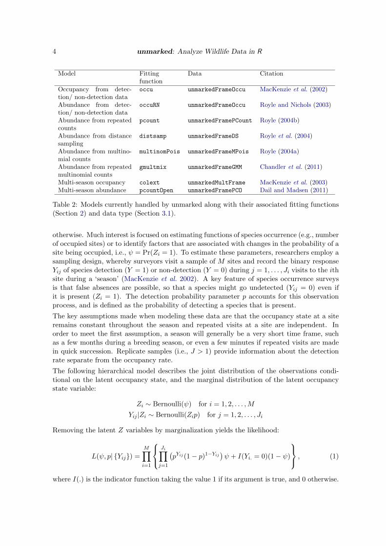
The list of models implemented in unmarked continues to grow as new models are developed.Table 2 shows the models available as of version 0.9-0. Rather than describe each fittingfunction in detail, this section provides a summary of several of the most common samplingtechniques and how unmarked can be used to model the resulting data.
2.1. Site occupancy models
Single season site occupancy model
An important state variable in ecological research is species occurrence (or ‘site occupancy’),say Zi, a binary state variable such that Zi = 1 if site i is occupied by a species and Zi = 0
4 unmarked: Analyze Wildlife Data in R
Model Fitting Data Citationfunction
Occupancy from detec-tion/ non-detection data
occu unmarkedFrameOccu MacKenzie et al. (2002)
Abundance from detec-tion/ non-detection data
occuRN unmarkedFrameOccu Royle and Nichols (2003)
Abundance from repeatedcounts
pcount unmarkedFramePCount Royle (2004b)
Abundance from distancesampling
distsamp unmarkedFrameDS Royle et al. (2004)
Abundance from multino-mial counts
multinomPois unmarkedFrameMPois Royle (2004a)
Abundance from repeatedmultinomial counts
gmultmix unmarkedFrameGMM Chandler et al. (2011)
Multi-season occupancy colext unmarkedMultFrame MacKenzie et al. (2003)Multi-season abundance pcountOpen unmarkedFramePCO Dail and Madsen (2011)
Table 2: Models currently handled by unmarked along with their associated fitting functions(Section 2) and data type (Section 3.1).
otherwise. Much interest is focused on estimating functions of species occurrence (e.g., numberof occupied sites) or to identify factors that are associated with changes in the probability of asite being occupied, i.e., ψ = Pr(Zi = 1). To estimate these parameters, researchers employ asampling design, whereby surveyors visit a sample of M sites and record the binary responseYij of species detection (Y = 1) or non-detection (Y = 0) during j = 1, . . . , Ji visits to the ithsite during a ‘season’ (MacKenzie et al. 2002). A key feature of species occurrence surveysis that false absences are possible, so that a species might go undetected (Yij = 0) even ifit is present (Zi = 1). The detection probability parameter p accounts for this observationprocess, and is defined as the probability of detecting a species that is present.
The key assumptions made when modeling these data are that the occupancy state at a siteremains constant throughout the season and repeated visits at a site are independent. Inorder to meet the first assumption, a season will generally be a very short time frame, suchas a few months during a breeding season, or even a few minutes if repeated visits are madein quick succession. Replicate samples (i.e., J > 1) provide information about the detectionrate separate from the occupancy rate.
The following hierarchical model describes the joint distribution of the observations condi-tional on the latent occupancy state, and the marginal distribution of the latent occupancystate variable:
Zi ∼ Bernoulli(ψ) for i = 1, 2, . . . ,M
Yij |Zi ∼ Bernoulli(Zip) for j = 1, 2, . . . , Ji
Removing the latent Z variables by marginalization yields the likelihood:
L(ψ, p| {Yij}) =M∏i=1
Ji∏j=1
(pYij (1− p)1−Yij
)ψ + I(Yi. = 0)(1− ψ)
, (1)
where I(.) is the indicator function taking the value 1 if its argument is true, and 0 otherwise.
Journal of Statistical Software 5
The model and likelihood are easily generalizable to accommodate covariates on detectionprobability or occupancy. Variables that are related to the occupancy state are modeled as
logit(ψi) = x>i β,
where xi is a vector of site-level covariates and β is a vector of their corresponding effectparameters. Similarly, the probability of detection can be modeled with
logit(pij) = v>ijα,
where vij is a vector of observation-level covariates and α is a vector of their correspondingeffect parameters. Examples of site-level covariates include habitat characteristics such asvegetation height. Observation-level covariates could include time of day, date, wind speed,or other factors that might affect detection probability. The function occu implements thismodel.
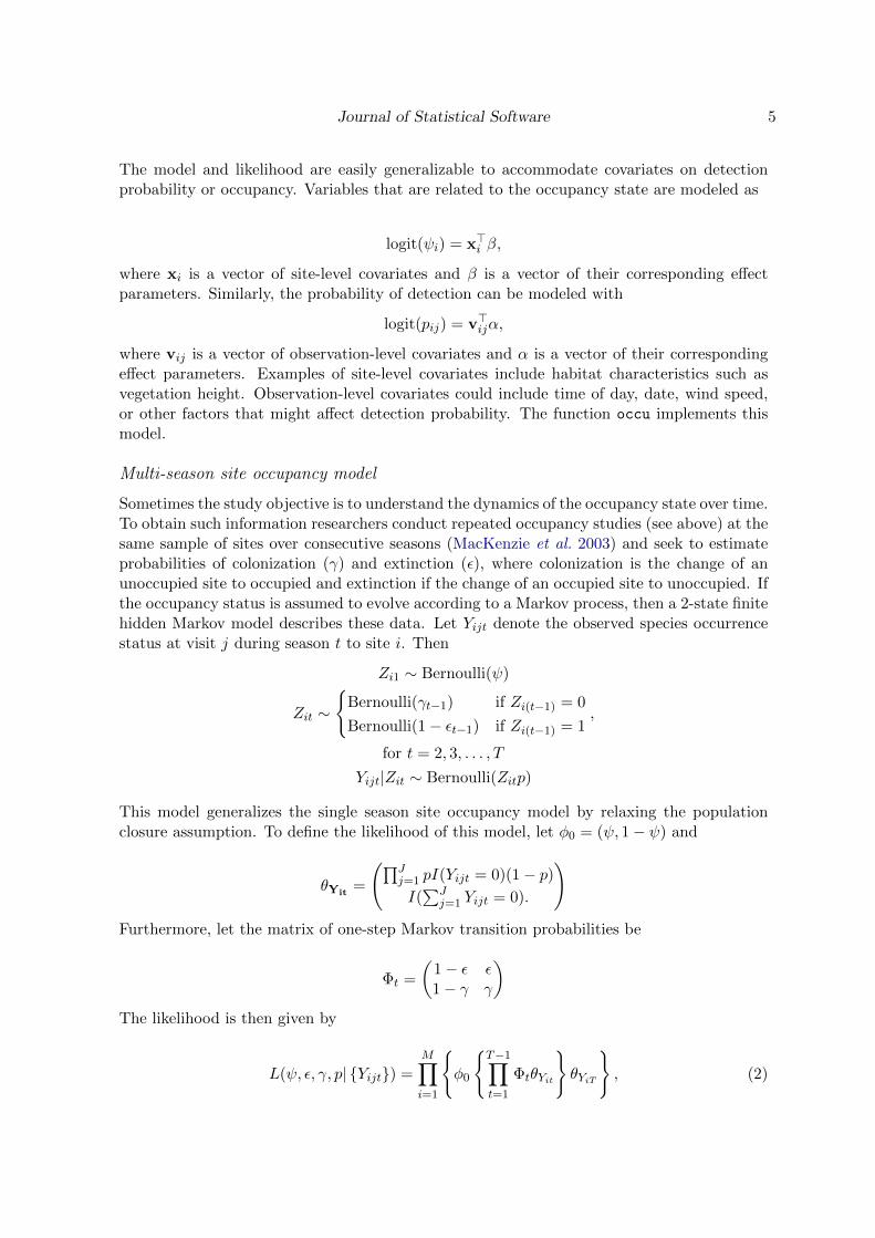
Multi-season site occupancy model
Sometimes the study objective is to understand the dynamics of the occupancy state over time.To obtain such information researchers conduct repeated occupancy studies (see above) at thesame sample of sites over consecutive seasons (MacKenzie et al. 2003) and seek to estimateprobabilities of colonization (γ) and extinction (ε), where colonization is the change of anunoccupied site to occupied and extinction if the change of an occupied site to unoccupied. Ifthe occupancy status is assumed to evolve according to a Markov process, then a 2-state finitehidden Markov model describes these data. Let Yijt denote the observed species occurrencestatus at visit j during season t to site i. Then
Zi1 ∼ Bernoulli(ψ)
Zit ∼
{Bernoulli(γt−1) if Zi(t−1) = 0
Bernoulli(1− εt−1) if Zi(t−1) = 1,
for t = 2, 3, . . . , T
Yijt|Zit ∼ Bernoulli(Zitp)
This model generalizes the single season site occupancy model by relaxing the populationclosure assumption. To define the likelihood of this model, let φ0 = (ψ, 1− ψ) and
θYit=
(∏Jj=1 pI(Yijt = 0)(1− p)I(∑J
j=1 Yijt = 0).
)Furthermore, let the matrix of one-step Markov transition probabilities be
Φt =
(1− ε ε1− γ γ
)The likelihood is then given by
L(ψ, ε, γ, p| {Yijt}) =M∏i=1
{φ0
{T−1∏t=1
ΦtθYit
}θYiT
}, (2)
6 unmarked: Analyze Wildlife Data in R
which can be maximized by the colext function in unmarked. Again, each of the four modelparameters ψ, γ, ε, and p can be modeled as functions of covariates on the logit scale.
2.2. Abundance models
Repeated count data
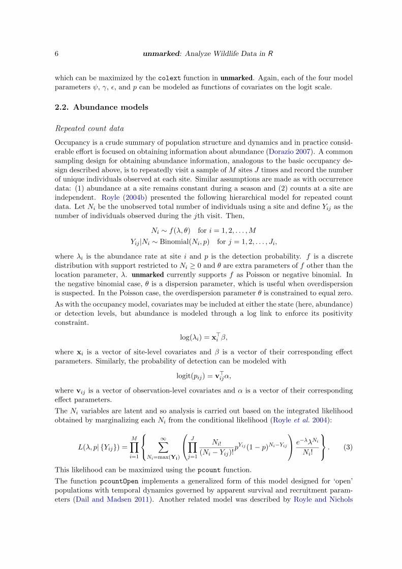
Occupancy is a crude summary of population structure and dynamics and in practice consid-erable effort is focused on obtaining information about abundance (Dorazio 2007). A commonsampling design for obtaining abundance information, analogous to the basic occupancy de-sign described above, is to repeatedly visit a sample of M sites J times and record the numberof unique individuals observed at each site. Similar assumptions are made as with occurrencedata: (1) abundance at a site remains constant during a season and (2) counts at a site areindependent. Royle (2004b) presented the following hierarchical model for repeated countdata. Let Ni be the unobserved total number of individuals using a site and define Yij as thenumber of individuals observed during the jth visit. Then,
Ni ∼ f(λ, θ) for i = 1, 2, . . . ,M
Yij |Ni ∼ Binomial(Ni, p) for j = 1, 2, . . . , Ji,
where λi is the abundance rate at site i and p is the detection probability. f is a discretedistribution with support restricted to Ni ≥ 0 and θ are extra parameters of f other than thelocation parameter, λ. unmarked currently supports f as Poisson or negative binomial. Inthe negative binomial case, θ is a dispersion parameter, which is useful when overdispersionis suspected. In the Poisson case, the overdispersion parameter θ is constrained to equal zero.
As with the occupancy model, covariates may be included at either the state (here, abundance)or detection levels, but abundance is modeled through a log link to enforce its positivityconstraint.
log(λi) = x>i β,
where xi is a vector of site-level covariates and β is a vector of their corresponding effectparameters. Similarly, the probability of detection can be modeled with
logit(pij) = v>ijα,
where vij is a vector of observation-level covariates and α is a vector of their correspondingeffect parameters.
The Ni variables are latent and so analysis is carried out based on the integrated likelihoodobtained by marginalizing each Ni from the conditional likelihood (Royle et al. 2004):
L(λ, p| {Yij}) =M∏i=1
∞∑
Ni=max(Yi)
J∏j=1
Ni!
(Ni − Yij)!pYij (1− p)Ni−Yij
e−λλNi
Ni!
. (3)
This likelihood can be maximized using the pcount function.
The function pcountOpen implements a generalized form of this model designed for ‘open’populations with temporal dynamics governed by apparent survival and recruitment param-eters (Dail and Madsen 2011). Another related model was described by Royle and Nichols
Journal of Statistical Software 7
(2003) and can be fit with the occuRN function. This model estimates abundance from siteoccupancy data by exploiting the link between abundance and detection probability.
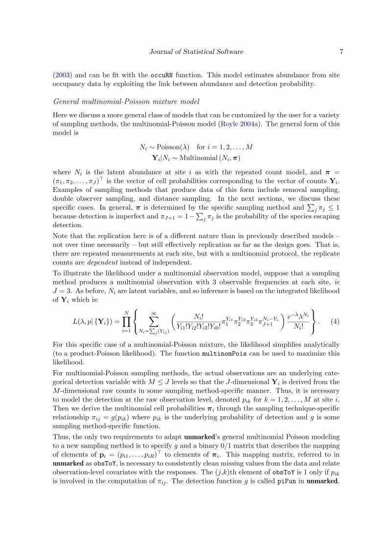
General multinomial-Poisson mixture model
Here we discuss a more general class of models that can be customized by the user for a varietyof sampling methods, the multinomial-Poisson model (Royle 2004a). The general form of thismodel is
Ni ∼ Poisson(λ) for i = 1, 2, . . . ,M
Yi|Ni ∼ Multinomial (Ni,π)
where Ni is the latent abundance at site i as with the repeated count model, and π =(π1, π2, . . . , πJ)> is the vector of cell probabilities corresponding to the vector of counts Yi.Examples of sampling methods that produce data of this form include removal sampling,double observer sampling, and distance sampling. In the next sections, we discuss thesespecific cases. In general, π is determined by the specific sampling method and
∑j πj ≤ 1
because detection is imperfect and πJ+1 = 1−∑
j πj is the probability of the species escapingdetection.
Note that the replication here is of a different nature than in previously described models –not over time necessarily – but still effectively replication as far as the design goes. That is,there are repeated measurements at each site, but with a multinomial protocol, the replicatecounts are dependent instead of independent.
To illustrate the likelihood under a multinomial observation model, suppose that a samplingmethod produces a multinomial observation with 3 observable frequencies at each site, ieJ = 3. As before, Ni are latent variables, and so inference is based on the integrated likelihoodof Yi which is:
L(λ, p| {Yi}) =
N∏i=1
∞∑
Ni=∑
j(Yij)
(Ni!
Yi1!Yi2!Yi3!Yi0!πYi11 πYi22 πYi33 πNi−Yi.
J+1
)e−λλNi
Ni!
. (4)
For this specific case of a multinomial-Poisson mixture, the likelihood simplifies analytically(to a product-Poisson likelihood). The function multinomPois can be used to maximize thislikelihood.
For multinomial-Poisson sampling methods, the actual observations are an underlying cate-gorical detection variable with M ≤ J levels so that the J-dimensional Yi is derived from theM -dimensional raw counts in some sampling method-specific manner. Thus, it is necessaryto model the detection at the raw observation level, denoted pik for k = 1, 2, . . . ,M at site i.Then we derive the multinomial cell probabilities πi through the sampling technique-specificrelationship πij = g(pik) where pik is the underlying probability of detection and g is somesampling method-specific function.
Thus, the only two requirements to adapt unmarked’s general multinomial Poisson modelingto a new sampling method is to specify g and a binary 0/1 matrix that describes the mappingof elements of pi = (pi1, . . . , piR)> to elements of πi. This mapping matrix, referred to inunmarked as obsToY, is necessary to consistently clean missing values from the data and relateobservation-level covariates with the responses. The (j,k)th element of obsToY is 1 only if pikis involved in the computation of πij . The detection function g is called piFun in unmarked.
8 unmarked: Analyze Wildlife Data in R
Covariates may be included in either the state (here, abundance) or detection models, throughpi (not πi).
log(λi) = x>i β,
where xi is a vector of site-level covariates and β is a vector of their corresponding effectparameters. Similarly, the probability of detection can be modeled with
logit(pij) = v>ijα,
where vij is a vector of observation-level covariates and α is a vector of their correspondingeffect parameters.
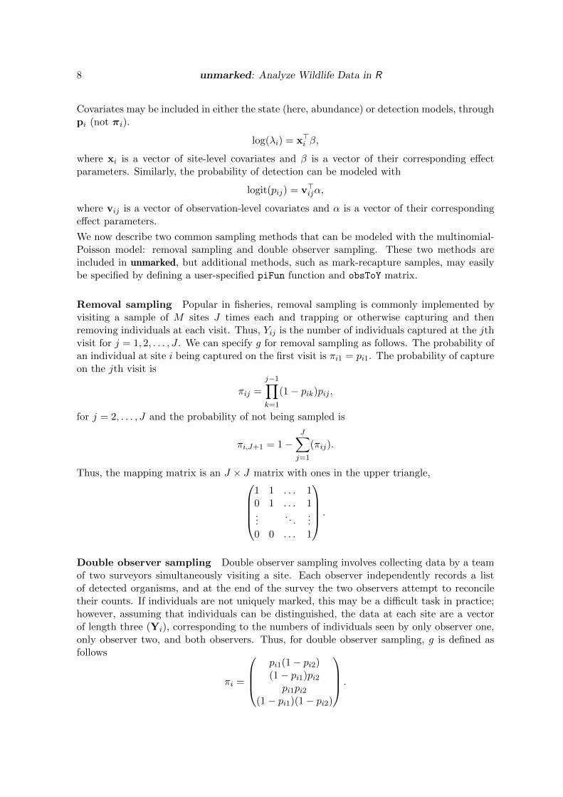
We now describe two common sampling methods that can be modeled with the multinomial-Poisson model: removal sampling and double observer sampling. These two methods areincluded in unmarked, but additional methods, such as mark-recapture samples, may easilybe specified by defining a user-specified piFun function and obsToY matrix.
Removal sampling Popular in fisheries, removal sampling is commonly implemented byvisiting a sample of M sites J times each and trapping or otherwise capturing and thenremoving individuals at each visit. Thus, Yij is the number of individuals captured at the jthvisit for j = 1, 2, . . . , J . We can specify g for removal sampling as follows. The probability ofan individual at site i being captured on the first visit is πi1 = pi1. The probability of captureon the jth visit is
πij =
j−1∏k=1
(1− pik)pij ,
for j = 2, . . . , J and the probability of not being sampled is
πi,J+1 = 1−J∑j=1
(πij).
Thus, the mapping matrix is an J × J matrix with ones in the upper triangle,1 1 . . . 10 1 . . . 1...
. . ....
0 0 . . . 1
.
Double observer sampling Double observer sampling involves collecting data by a teamof two surveyors simultaneously visiting a site. Each observer independently records a listof detected organisms, and at the end of the survey the two observers attempt to reconciletheir counts. If individuals are not uniquely marked, this may be a difficult task in practice;however, assuming that individuals can be distinguished, the data at each site are a vectorof length three (Yi), corresponding to the numbers of individuals seen by only observer one,only observer two, and both observers. Thus, for double observer sampling, g is defined asfollows
πi =
pi1(1− pi2)(1− pi1)pi2pi1pi2
(1− pi1)(1− pi2)
.
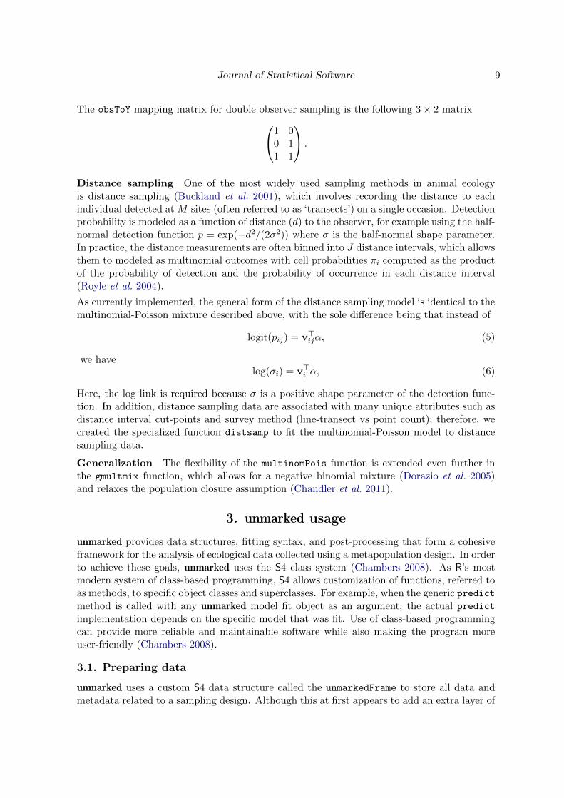
Journal of Statistical Software 9
The obsToY mapping matrix for double observer sampling is the following 3× 2 matrix1 00 11 1
.
Distance sampling One of the most widely used sampling methods in animal ecologyis distance sampling (Buckland et al. 2001), which involves recording the distance to eachindividual detected at M sites (often referred to as ‘transects’) on a single occasion. Detectionprobability is modeled as a function of distance (d) to the observer, for example using the half-normal detection function p = exp(−d2/(2σ2)) where σ is the half-normal shape parameter.In practice, the distance measurements are often binned into J distance intervals, which allowsthem to modeled as multinomial outcomes with cell probabilities πi computed as the productof the probability of detection and the probability of occurrence in each distance interval(Royle et al. 2004).
As currently implemented, the general form of the distance sampling model is identical to themultinomial-Poisson mixture described above, with the sole difference being that instead of
logit(pij) = v>ijα, (5)
we havelog(σi) = v>i α, (6)
Here, the log link is required because σ is a positive shape parameter of the detection func-tion. In addition, distance sampling data are associated with many unique attributes such asdistance interval cut-points and survey method (line-transect vs point count); therefore, wecreated the specialized function distsamp to fit the multinomial-Poisson model to distancesampling data.
Generalization The flexibility of the multinomPois function is extended even further inthe gmultmix function, which allows for a negative binomial mixture (Dorazio et al. 2005)and relaxes the population closure assumption (Chandler et al. 2011).
3. unmarked usage
unmarked provides data structures, fitting syntax, and post-processing that form a cohesiveframework for the analysis of ecological data collected using a metapopulation design. In orderto achieve these goals, unmarked uses the S4 class system (Chambers 2008). As R’s mostmodern system of class-based programming, S4 allows customization of functions, referred toas methods, to specific object classes and superclasses. For example, when the generic predictmethod is called with any unmarked model fit object as an argument, the actual predictimplementation depends on the specific model that was fit. Use of class-based programmingcan provide more reliable and maintainable software while also making the program moreuser-friendly (Chambers 2008).
3.1. Preparing data
unmarked uses a custom S4 data structure called the unmarkedFrame to store all data andmetadata related to a sampling design. Although this at first appears to add an extra layer of
10 unmarked: Analyze Wildlife Data in R
work for the user, there are several reasons for this design choice. The multilevel structure ofthe models means that standard rectangular data structures such as data.frames or matricesare not suitable for storing the data. For example, covariates might have been measuredseparately at the site level and at the visit level. Furthermore, the length of the response vectorYi at site i might differ from the number of observations at the site as in the multinomialPoisson model. In some cases, metadata of arbitrary dimensions may need to be associatedwith the data. For example, in distance sampling it is necessary to store the units of measureand the survey design type. Aside from these technical reasons, Gentleman (2009) pointedout that the use of such portable custom data objects can simplify future reference to previousanalyses, an often neglected aspect of research. Repeated fitting calls using the same set ofdata require less code repetition if all data are contained in a single object. Finally, calls tofitting functions have a cleaner appearance with a more obvious purpose when the call is notburied in data arguments.
The parent S4 data class is called an unmarkedFrame and each unmarked fitting functionhas its own data type that extends the unmarkedFrame. To ease data importing and con-version, unmarked includes several helper functions to automatically convert data into anunmarkedFrame: csvToUMF which imports data directly from a comma-separated value textfile, formatWide and formatLong which convert data from data frames, and the family ofunmarkedFrame constructor functions.
An unmarkedFrame object contains components, referred to as slots, which hold the dataand metadata. All unmarkedFrame objects contain a slot for the observation matrix y, adata.frame of site-level covariates siteCovs, and a data.frame of observation-level covari-ates obsCovs. The y matrix is the only required slot. Each row of y contains either the ob-served counts or detection/non-detection data at each of the M sites. siteCovs is an M -rowdata.frame with a column for each site-level covariate. obsCovs is an MJ-row data.frame
with a column for each observation-level covariate. Thus each row of obsCovs corresponds toa particular observation, with the order corresponding to site varying slower and observationwithin site varying faster. Both siteCovs and obsCovs can contain NA values correspondingto unbalanced or missing data. If a site-level covariate is missing, unmarked automaticallyremoves all data for that site prior to fitting the model. Missing values in the obsCovs arehandled by removing the corresponding occurrence or count observations such that the miss-ing values make no contribution to the likelihood. unmarked provides constructor functionsto make creating unmarkedFrames straightforward. For each specific data type, specific typesof unmarkedFrames extend the basic unmarkedFrame to handle model-specific nuances.
Importing repeated count data
Here is an example of creating an unmarkedFrame for repeated count data (Section 2.2). First,load Mallard (Anas platyrhynchos) point count dataset described in Kery et al. (2005).
R> library("unmarked")
R> data("mallard")
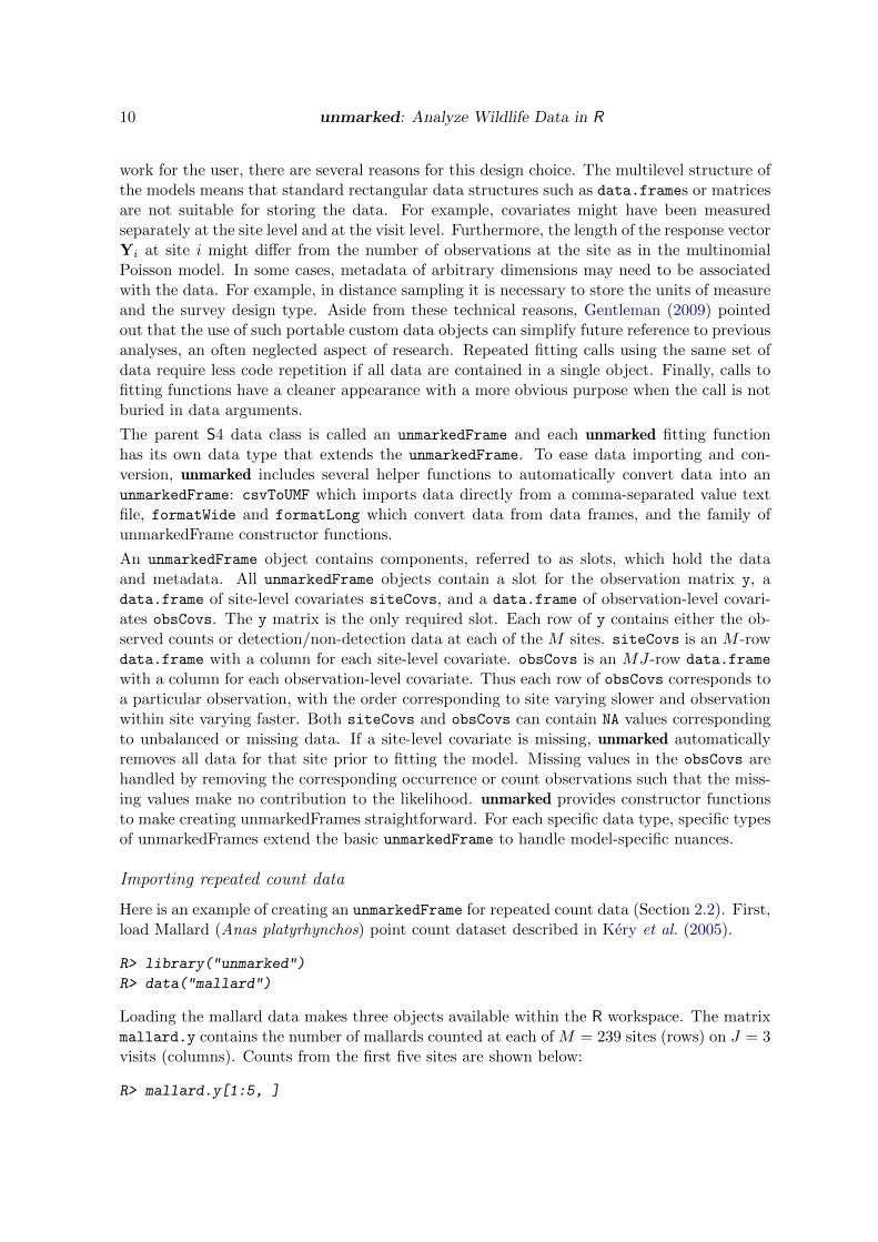
Loading the mallard data makes three objects available within the R workspace. The matrixmallard.y contains the number of mallards counted at each of M = 239 sites (rows) on J = 3visits (columns). Counts from the first five sites are shown below:
R> mallard.y[1:5, ]
Journal of Statistical Software 11
y.1 y.2 y.3
[1,] 0 0 0
[2,] 0 0 0
[3,] 3 2 1
[4,] 0 0 0
[5,] 3 0 3
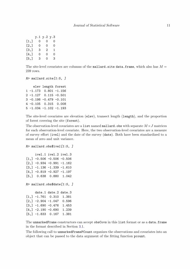
The site-level covariates are columns of the mallard.site data.frame, which also has M =239 rows.
R> mallard.site[1:5, ]
elev length forest
1 -1.173 0.801 -1.156
2 -1.127 0.115 -0.501
3 -0.198 -0.479 -0.101
4 -0.105 0.315 0.008
5 -1.034 -1.102 -1.193
The site-level covariates are elevation (elev), transect length (length), and the proportionof forest covering the site (forest).
The observation-level covariates are a list named mallard.obs with separate M×J matricesfor each observation-level covariate. Here, the two observation-level covariates are a measureof survey effort (ivel) and the date of the survey (date). Both have been standardized to amean of zero and unit variance.
R> mallard.obs$ivel[1:5, ]
ivel.1 ivel.2 ivel.3
[1,] -0.506 -0.506 -0.506
[2,] -0.934 -0.991 -1.162
[3,] -1.136 -1.339 -1.610
[4,] -0.819 -0.927 -1.197
[5,] 0.638 0.880 1.042
R> mallard.obs$date[1:5, ]
date.1 date.2 date.3
[1,] -1.761 0.310 1.381
[2,] -2.904 -1.047 0.596
[3,] -1.690 -0.476 1.453
[4,] -2.190 -0.690 1.239
[5,] -1.833 0.167 1.381
The unmarkedFrame constructors can accept obsCovs in this list format or as a data.frame
in the format described in Section 3.1.
The following call to unmarkedFramePCount organizes the observations and covariates into anobject that can be passed to the data argument of the fitting function pcount.
12 unmarked: Analyze Wildlife Data in R
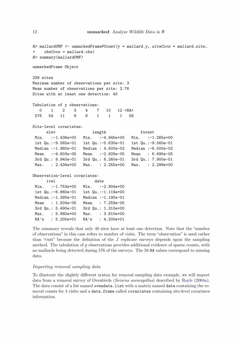
R> mallardUMF <- unmarkedFramePCount(y = mallard.y, siteCovs = mallard.site,
+ obsCovs = mallard.obs)
R> summary(mallardUMF)
unmarkedFrame Object
239 sites
Maximum number of observations per site: 3
Mean number of observations per site: 2.76
Sites with at least one detection: 40
Tabulation of y observations:
0 1 2 3 4 7 10 12 <NA>
576 54 11 9 6 1 1 1 58
Site-level covariates:
elev length forest
Min. :-1.436e+00 Min. :-4.945e+00 Min. :-1.265e+00
1st Qu.:-9.565e-01 1st Qu.:-5.630e-01 1st Qu.:-9.560e-01
Median :-1.980e-01 Median : 4.500e-02 Median :-6.500e-02
Mean :-4.603e-05 Mean :-2.929e-05 Mean : 6.695e-05
3rd Qu.: 9.940e-01 3rd Qu.: 6.260e-01 3rd Qu.: 7.900e-01
Max. : 2.434e+00 Max. : 2.255e+00 Max. : 2.299e+00
Observation-level covariates:
ivel date
Min. :-1.753e+00 Min. :-2.904e+00
1st Qu.:-6.660e-01 1st Qu.:-1.119e+00
Median :-1.390e-01 Median :-1.190e-01
Mean : 1.504e-05 Mean : 7.259e-05
3rd Qu.: 5.490e-01 3rd Qu.: 1.310e+00
Max. : 5.980e+00 Max. : 3.810e+00
NA's : 5.200e+01 NA's : 4.200e+01
The summary reveals that only 40 sites have at least one detection. Note that the “numberof observations” in this case refers to number of visits. The term “observation” is used ratherthan “visit” because the definition of the J replicate surveys depends upon the samplingmethod. The tabulation of y observations provides additional evidence of sparse counts, withno mallards being detected during 576 of the surveys. The 58 NA values correspond to missingdata.
Importing removal sampling data
To illustrate the slightly different syntax for removal sampling data example, we will importdata from a removal survey of Ovenbirds (Seiurus aurocapillus) described by Royle (2004a).The data consist of a list named ovendata.list with a matrix named data containing the re-moval counts for 4 visits and a data.frame called covariates containing site-level covariatesinformation.
Journal of Statistical Software 13
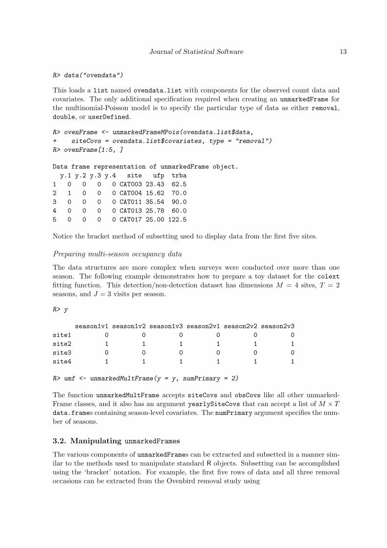
R> data("ovendata")
This loads a list named ovendata.list with components for the observed count data andcovariates. The only additional specification required when creating an unmarkedFrame forthe multinomial-Poisson model is to specify the particular type of data as either removal,double, or userDefined.
R> ovenFrame <- unmarkedFrameMPois(ovendata.list$data,
+ siteCovs = ovendata.list$covariates, type = "removal")
R> ovenFrame[1:5, ]
Data frame representation of unmarkedFrame object.
y.1 y.2 y.3 y.4 site ufp trba
1 0 0 0 0 CAT003 23.43 62.5
2 1 0 0 0 CAT004 15.62 70.0
3 0 0 0 0 CAT011 35.54 90.0
4 0 0 0 0 CAT013 25.78 60.0
5 0 0 0 0 CAT017 25.00 122.5
Notice the bracket method of subsetting used to display data from the first five sites.
Preparing multi-season occupancy data
The data structures are more complex when surveys were conducted over more than oneseason. The following example demonstrates how to prepare a toy dataset for the colext
fitting function. This detection/non-detection dataset has dimensions M = 4 sites, T = 2seasons, and J = 3 visits per season.
R> y
season1v1 season1v2 season1v3 season2v1 season2v2 season2v3
site1 0 0 0 0 0 0
site2 1 1 1 1 1 1
site3 0 0 0 0 0 0
site4 1 1 1 1 1 1
R> umf <- unmarkedMultFrame(y = y, numPrimary = 2)
The function unmarkedMultFrame accepts siteCovs and obsCovs like all other unmarked-Frame classes, and it also has an argument yearlySiteCovs that can accept a list of M × Tdata.frames containing season-level covariates. The numPrimary argument specifies the num-ber of seasons.
3.2. Manipulating unmarkedFrames
The various components of unmarkedFrames can be extracted and subsetted in a manner sim-ilar to the methods used to manipulate standard R objects. Subsetting can be accomplishedusing the ‘bracket’ notation. For example, the first five rows of data and all three removaloccasions can be extracted from the Ovenbird removal study using
14 unmarked: Analyze Wildlife Data in R
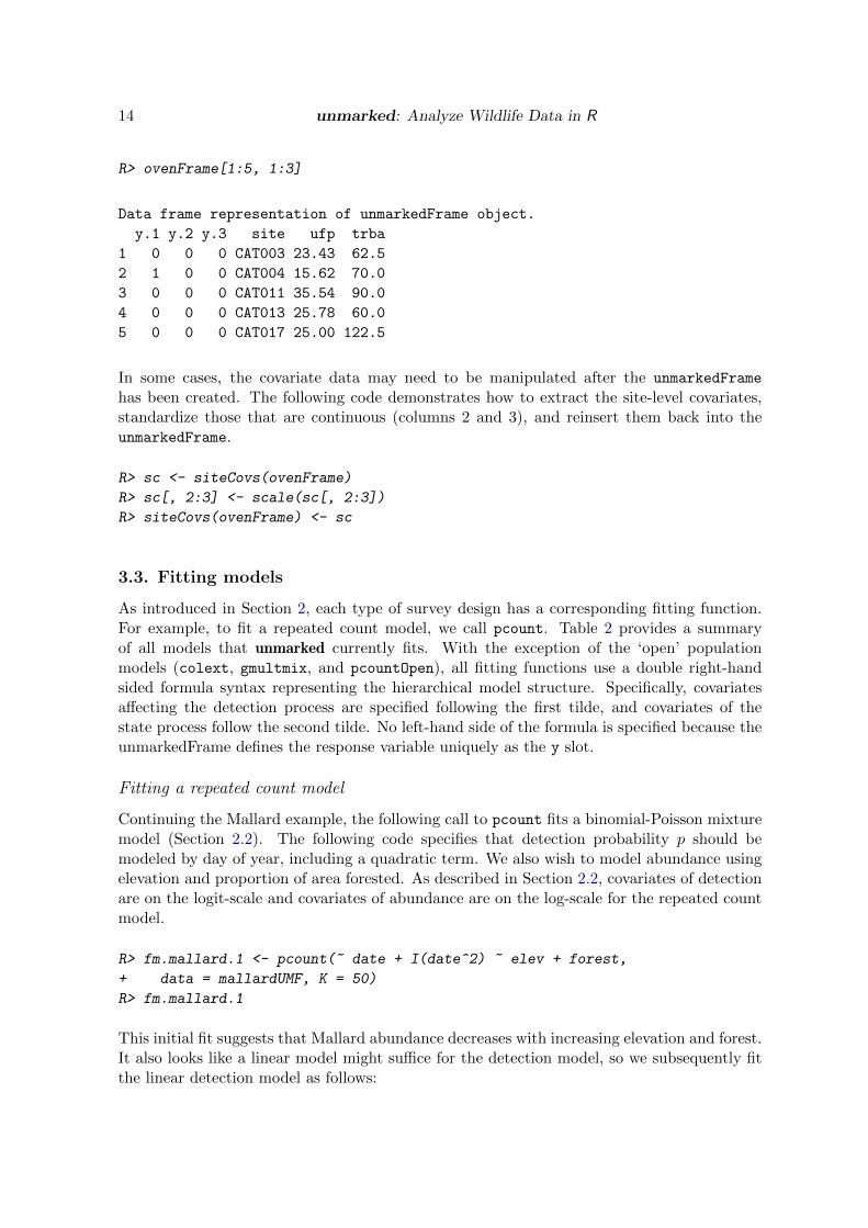
R> ovenFrame[1:5, 1:3]
Data frame representation of unmarkedFrame object.
y.1 y.2 y.3 site ufp trba
1 0 0 0 CAT003 23.43 62.5
2 1 0 0 CAT004 15.62 70.0
3 0 0 0 CAT011 35.54 90.0
4 0 0 0 CAT013 25.78 60.0
5 0 0 0 CAT017 25.00 122.5
In some cases, the covariate data may need to be manipulated after the unmarkedFrame
has been created. The following code demonstrates how to extract the site-level covariates,standardize those that are continuous (columns 2 and 3), and reinsert them back into theunmarkedFrame.
R> sc <- siteCovs(ovenFrame)
R> sc[, 2:3] <- scale(sc[, 2:3])
R> siteCovs(ovenFrame) <- sc
3.3. Fitting models
As introduced in Section 2, each type of survey design has a corresponding fitting function.For example, to fit a repeated count model, we call pcount. Table 2 provides a summaryof all models that unmarked currently fits. With the exception of the ‘open’ populationmodels (colext, gmultmix, and pcountOpen), all fitting functions use a double right-handsided formula syntax representing the hierarchical model structure. Specifically, covariatesaffecting the detection process are specified following the first tilde, and covariates of thestate process follow the second tilde. No left-hand side of the formula is specified because theunmarkedFrame defines the response variable uniquely as the y slot.
Fitting a repeated count model
Continuing the Mallard example, the following call to pcount fits a binomial-Poisson mixturemodel (Section 2.2). The following code specifies that detection probability p should bemodeled by day of year, including a quadratic term. We also wish to model abundance usingelevation and proportion of area forested. As described in Section 2.2, covariates of detectionare on the logit-scale and covariates of abundance are on the log-scale for the repeated countmodel.
R> fm.mallard.1 <- pcount(~ date + I(date^2) ~ elev + forest,
+ data = mallardUMF, K = 50)
R> fm.mallard.1
This initial fit suggests that Mallard abundance decreases with increasing elevation and forest.It also looks like a linear model might suffice for the detection model, so we subsequently fitthe linear detection model as follows:
Journal of Statistical Software 15
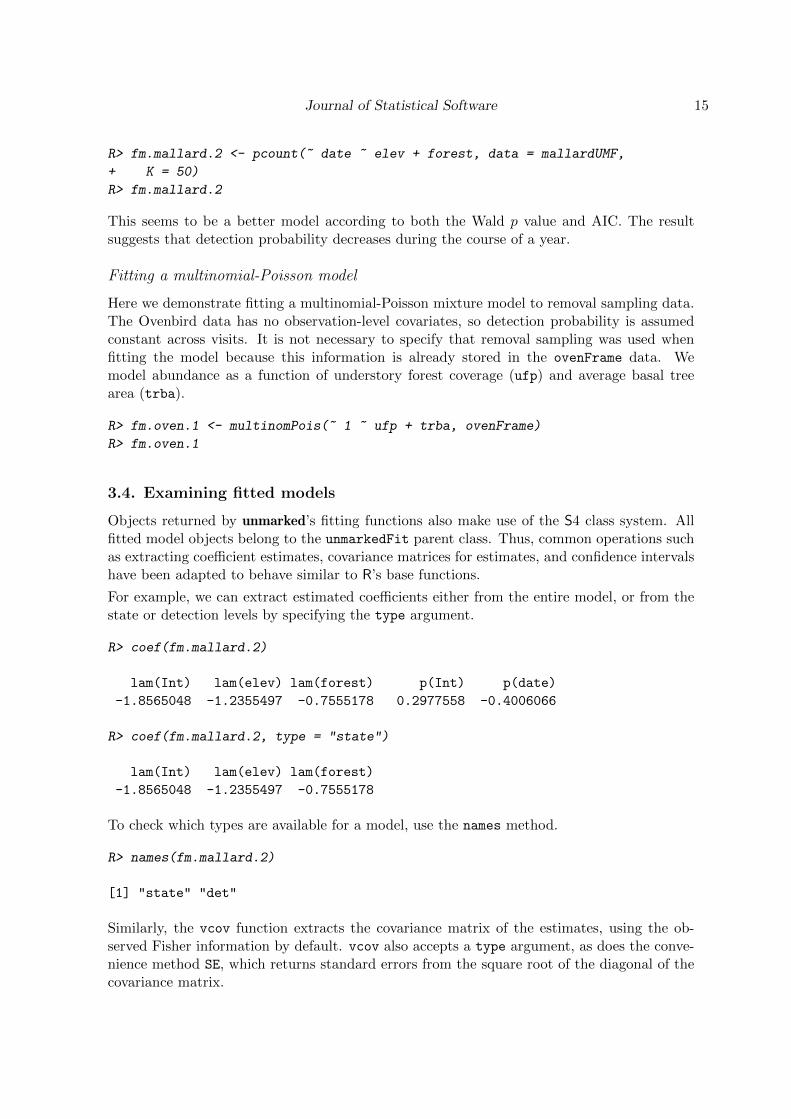
R> fm.mallard.2 <- pcount(~ date ~ elev + forest, data = mallardUMF,
+ K = 50)
R> fm.mallard.2
This seems to be a better model according to both the Wald p value and AIC. The resultsuggests that detection probability decreases during the course of a year.
Fitting a multinomial-Poisson model
Here we demonstrate fitting a multinomial-Poisson mixture model to removal sampling data.The Ovenbird data has no observation-level covariates, so detection probability is assumedconstant across visits. It is not necessary to specify that removal sampling was used whenfitting the model because this information is already stored in the ovenFrame data. Wemodel abundance as a function of understory forest coverage (ufp) and average basal treearea (trba).
R> fm.oven.1 <- multinomPois(~ 1 ~ ufp + trba, ovenFrame)
R> fm.oven.1
3.4. Examining fitted models
Objects returned by unmarked’s fitting functions also make use of the S4 class system. Allfitted model objects belong to the unmarkedFit parent class. Thus, common operations suchas extracting coefficient estimates, covariance matrices for estimates, and confidence intervalshave been adapted to behave similar to R’s base functions.
For example, we can extract estimated coefficients either from the entire model, or from thestate or detection levels by specifying the type argument.
R> coef(fm.mallard.2)
lam(Int) lam(elev) lam(forest) p(Int) p(date)
-1.8565048 -1.2355497 -0.7555178 0.2977558 -0.4006066
R> coef(fm.mallard.2, type = "state")
lam(Int) lam(elev) lam(forest)
-1.8565048 -1.2355497 -0.7555178
To check which types are available for a model, use the names method.
R> names(fm.mallard.2)
[1] "state" "det"
Similarly, the vcov function extracts the covariance matrix of the estimates, using the ob-served Fisher information by default. vcov also accepts a type argument, as does the conve-nience method SE, which returns standard errors from the square root of the diagonal of thecovariance matrix.
16 unmarked: Analyze Wildlife Data in R
R> vcov(fm.mallard.2, type = "det")
p(Int) p(date)
p(Int) 0.03549024 0.00344853
p(date) 0.00344853 0.01302865
Extracting confidence intervals proceeds in a similar fashion. By default, the asymptoticnormal approximation is used.
R> confint(fm.oven.1, type = "state", level = 0.95)
0.025 0.975
lambda(Int) -0.1299722 0.33470834
lambda(ufp) -0.1471741 0.34776195
lambda(trba) -0.4361311 0.09440937
Profile confidence intervals are also available upon request. This can take some time, however,because for each parameter, a nested optimization within a root-finding algorithm is beingused to find the profile limit.
R> ci <- confint(fm.oven.1, type = "state", level = 0.95, method = "profile")
R> ci
0.025 0.975
lambda(Int) -0.1390786 0.32676614
lambda(ufp) -0.1477724 0.34811770
lambda(trba) -0.4368444 0.09469605
The profile confidence intervals and normal approximations are quite similar here.
The nonparametric bootstrap
Nonparametric bootstrapping can also be used to estimate the covariance matrix. unmarkedimplements a two-stage bootstrap in which the sites are first drawn with replacement, and thenwithin each site, the observations are drawn with replacement. First, bootstrap draws must betaken using the nonparboot function, which returns a new version of the unmarkedFit objectwith additional bootstrap sampling information. Thus, this new fit must be stored, either ina new fit object or the same one, and then subsequently queried for bootstrap summaries.To illustrate, we use the removal sampling data instead of the repeated count data becausecomputations are much faster; however, bootstrapping is available for any of the models inunmarked.
R> set.seed(1234)
R> fm.oven.1 <- nonparboot(fm.oven.1, B = 100)
R> SE(fm.oven.1, type = "state")
lambda(Int) lambda(ufp) lambda(trba)
0.1185431 0.1262615 0.1353444
Journal of Statistical Software 17
R> SE(fm.oven.1, type = "state", method = "nonparboot")
lambda(Int) lambda(ufp) lambda(trba)
0.1256949 0.1156153 0.1197142
The bootstrapping and asymptotic standard errors are similar. Additional bootstrap samplescan be drawn by calling nonparboot again.
R> fm.oven.1 <- nonparboot(fm.oven.1, B = 100)
Linear combinations of estimates
Often, meaningful hypotheses can be addressed by estimating linear combinations of coeffi-cient estimates. Linear combinations of coefficient estimates can be requested with linearComb.Continuing the Ovenbird example, the following code estimates the log-abundance rate for asite with ufp = 0.5 and trba= 0.
R> (lc <- linearComb(fm.oven.1, type = "state", coefficients = c(1, 0.5, 0)))
Linear combination(s) of Abundance estimate(s)
Estimate SE (Intercept) ufp trba
0.153 0.13 1 0.5 0
Multiple sets of coefficients may be supplied as a design matrix. The following code requeststhe estimated log-abundance for sites with ufp = 0.5 and trba = 1.
R> (lc <- linearComb(fm.oven.1, type = "state",
+ coefficients = matrix(c(1, 0.5, 0, 1, 1, 0), 2, 3, byrow = TRUE)))
Linear combination(s) of Abundance estimate(s)
Estimate SE (Intercept) ufp trba
1 0.153 0.130 1 0.5 0
2 0.203 0.166 1 1.0 0
Standard errors and confidence intervals are also available for linear combinations of parame-ters. By requesting nonparametric bootstrapped standard errors, unmarked uses the samplesthat were drawn earlier.
R> SE(lc, method = "nonparboot")
[1] 0.1354092 0.1659877
Back-transforming linear combinations of coefficients
Estimates of linear combinations back-transformed to the native scale are likely to be moreinteresting than the direct linear combinations. For example, the logistic transformation is
18 unmarked: Analyze Wildlife Data in R
applied to estimates of detection rates, resulting in a probability bound between 0 and 1. Thisis accomplished with the backTransform. Standard errors of back-transformed estimates areestimated using the delta method. Confidence intervals are estimated by back-transformingthe confidence interval of the original linear combination.
R> (btlc <- backTransform(lc))
Backtransformed linear combination(s) of Abundance estimate(s)
Estimate SE LinComb (Intercept) ufp trba
1 1.16 0.151 0.153 1 0.5 0
2 1.22 0.203 0.203 1 1.0 0
Transformation: exp
R> SE(btlc)
[1] 0.1510141 0.2032272
R> confint(btlc)
0.025 0.975
1 0.9033915 1.501747
2 0.8846296 1.695386
3.5. Model selection
unmarked performs AIC-based model selection for structured lists of unmarkedFit objects. Todemonstrate, we fit a few more models to the Ovenbird removal data, including an interactionmodel, two models with single predictors, and a model with no predictors.
R> fm.oven.2 <- update(fm.oven.1, formula = ~ 1 ~ ufp * trba)
R> fm.oven.3 <- update(fm.oven.1, formula = ~ 1 ~ ufp)
R> fm.oven.4 <- update(fm.oven.1, formula = ~ 1 ~ trba)
R> fm.oven.5 <- update(fm.oven.1, formula = ~ 1 ~ 1)
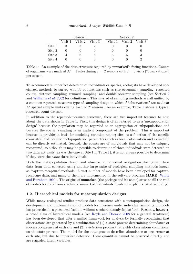
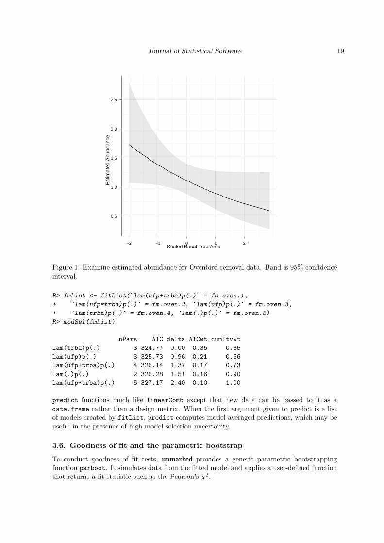
R> preddata <- predict(fm.oven.4, type = "state", appendData = TRUE)
R> library("ggplot2")
R> qplot(trba, Predicted, data = preddata, geom = "line",
+ xlab = "Scaled Basal Tree Area", ylab = "Estimated Abundance") +
+ geom_ribbon(aes(x = trba, ymin = lower, ymax = upper), alpha = 0.1) +
+ theme_bw()
It looks like the best model includes only tree basal area as a predictor of abundance. Wecan examine this relationship using the predict method and the ggplot2 package (Wickham2009), see Figure 1.
Next, we organize the fitted models with the fitList function and the use the modSel methodto rank the models by AIC.
Journal of Statistical Software 19
Scaled Basal Tree Area
Est
imat
ed A
bund
ance
0.5
1.0
1.5
2.0
2.5
−2 −1 0 1 2
Figure 1: Examine estimated abundance for Ovenbird removal data. Band is 95% confidenceinterval.
R> fmList <- fitList(`lam(ufp+trba)p(.)` = fm.oven.1,
+ `lam(ufp*trba)p(.)` = fm.oven.2, `lam(ufp)p(.)` = fm.oven.3,
+ `lam(trba)p(.)` = fm.oven.4, `lam(.)p(.)` = fm.oven.5)
R> modSel(fmList)
nPars AIC delta AICwt cumltvWt
lam(trba)p(.) 3 324.77 0.00 0.35 0.35
lam(ufp)p(.) 3 325.73 0.96 0.21 0.56
lam(ufp+trba)p(.) 4 326.14 1.37 0.17 0.73
lam(.)p(.) 2 326.28 1.51 0.16 0.90
lam(ufp*trba)p(.) 5 327.17 2.40 0.10 1.00
predict functions much like linearComb except that new data can be passed to it as adata.frame rather than a design matrix. When the first argument given to predict is a listof models created by fitList, predict computes model-averaged predictions, which may beuseful in the presence of high model selection uncertainty.
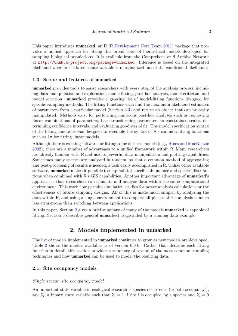
3.6. Goodness of fit and the parametric bootstrap
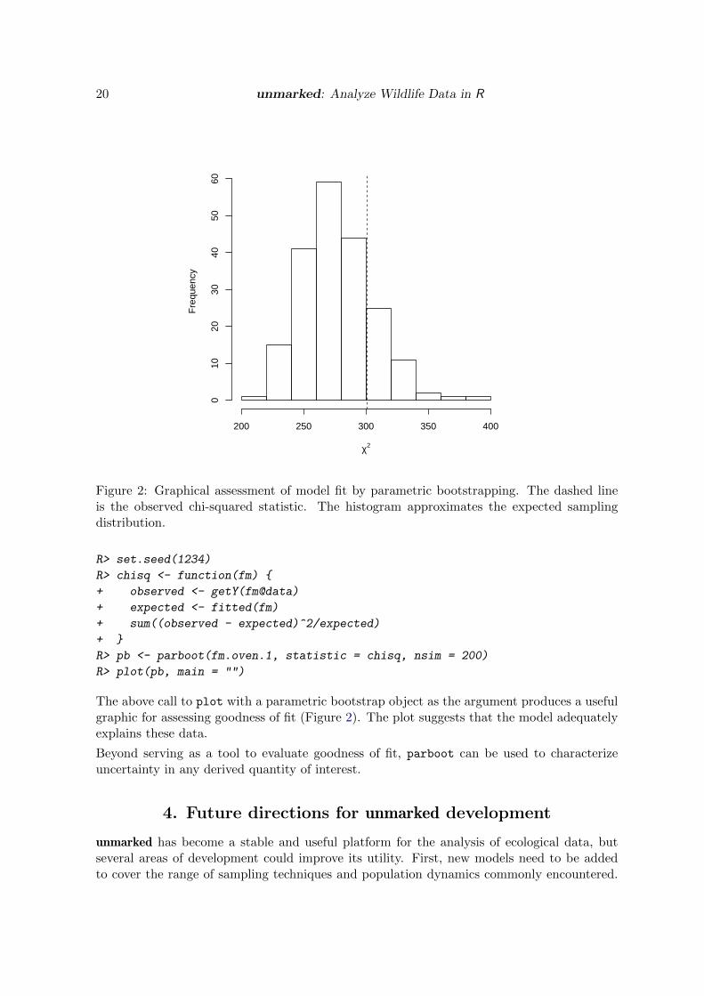
To conduct goodness of fit tests, unmarked provides a generic parametric bootstrappingfunction parboot. It simulates data from the fitted model and applies a user-defined functionthat returns a fit-statistic such as the Pearson’s χ2.
20 unmarked: Analyze Wildlife Data in R
χ2
Fre
quen
cy
200 250 300 350 400
010
2030
4050
60
Figure 2: Graphical assessment of model fit by parametric bootstrapping. The dashed lineis the observed chi-squared statistic. The histogram approximates the expected samplingdistribution.
R> set.seed(1234)
R> chisq <- function(fm) {
+ observed <- getY(fm@data)
+ expected <- fitted(fm)
+ sum((observed - expected)^2/expected)
+ }
R> pb <- parboot(fm.oven.1, statistic = chisq, nsim = 200)
R> plot(pb, main = "")
The above call to plot with a parametric bootstrap object as the argument produces a usefulgraphic for assessing goodness of fit (Figure 2). The plot suggests that the model adequatelyexplains these data.
Beyond serving as a tool to evaluate goodness of fit, parboot can be used to characterizeuncertainty in any derived quantity of interest.
4. Future directions for unmarked development
unmarked has become a stable and useful platform for the analysis of ecological data, butseveral areas of development could improve its utility. First, new models need to be addedto cover the range of sampling techniques and population dynamics commonly encountered.
Journal of Statistical Software 21
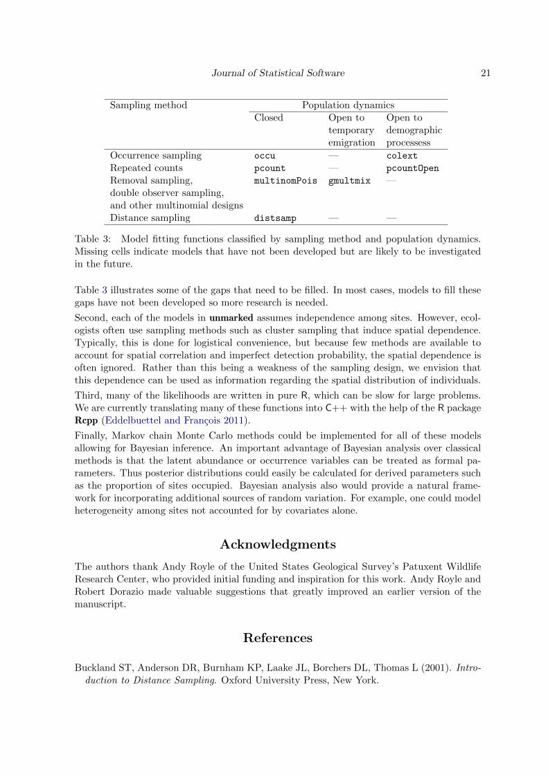
Sampling method Population dynamicsClosed Open to Open to
temporary demographicemigration processess
Occurrence sampling occu — colext
Repeated counts pcount — pcountOpen
Removal sampling, multinomPois gmultmix —double observer sampling,and other multinomial designsDistance sampling distsamp — —
Table 3: Model fitting functions classified by sampling method and population dynamics.Missing cells indicate models that have not been developed but are likely to be investigatedin the future.
Table 3 illustrates some of the gaps that need to be filled. In most cases, models to fill thesegaps have not been developed so more research is needed.
Second, each of the models in unmarked assumes independence among sites. However, ecol-ogists often use sampling methods such as cluster sampling that induce spatial dependence.Typically, this is done for logistical convenience, but because few methods are available toaccount for spatial correlation and imperfect detection probability, the spatial dependence isoften ignored. Rather than this being a weakness of the sampling design, we envision thatthis dependence can be used as information regarding the spatial distribution of individuals.
Third, many of the likelihoods are written in pure R, which can be slow for large problems.We are currently translating many of these functions into C++ with the help of the R packageRcpp (Eddelbuettel and Francois 2011).
Finally, Markov chain Monte Carlo methods could be implemented for all of these modelsallowing for Bayesian inference. An important advantage of Bayesian analysis over classicalmethods is that the latent abundance or occurrence variables can be treated as formal pa-rameters. Thus posterior distributions could easily be calculated for derived parameters suchas the proportion of sites occupied. Bayesian analysis also would provide a natural frame-work for incorporating additional sources of random variation. For example, one could modelheterogeneity among sites not accounted for by covariates alone.
Acknowledgments
The authors thank Andy Royle of the United States Geological Survey’s Patuxent WildlifeResearch Center, who provided initial funding and inspiration for this work. Andy Royle andRobert Dorazio made valuable suggestions that greatly improved an earlier version of themanuscript.
References
Buckland ST, Anderson DR, Burnham KP, Laake JL, Borchers DL, Thomas L (2001). Intro-duction to Distance Sampling. Oxford University Press, New York.
22 unmarked: Analyze Wildlife Data in R
Chambers JM (2008). Software for Data Analysis: Programming with R. Springer-Verlag,New York.
Chandler RB, Royle JA, King DI (2011). “Inference about Density and Temporary Emigrationin Unmarked Populations.” Ecology, 92(7).
Dail D, Madsen L (2011). “Models for Estimating Abundance from Repeated Counts of anOpen Metapopulation.” Biometrics, 67(2), 577–587.
Dorazio RM (2007). “On the Choice of Statistical Models for Estimating Occurrence andExtinction from Animal Surveys.” Ecology, 88(11), 2773–2782.
Dorazio RM, Jelks HL, Jordan F (2005). “Improving Removal-Based Estimates of Abundanceby Sampling a Population of Spatially Distinct Subpopulations.” Biometrics, 61(4), 1093–1101.
Eddelbuettel D, Francois R (2011). “Rcpp: Seamless R and C++ Integration.” Journal ofStatistical Software, 40(8), 1–18. URL http://www.jstatsoft.org/v40/i08/.
Gentleman R (2009). R Programming for Bioinformatics. Chapman & Hall/CRC, New York.
Hines JE, MacKenzie DI (2002). PRESENCE. USGS-PWRC, Laurel. URL http://www.
mbr-pwrc.usgs.gov/software/presence.html.
Kery M, Royle JA, Schmid H (2005). “Modeling Avian Abundance from Replicated CountsUsing Binomial Mixture Models.” Ecological Applications, 15(4), 1450–1461.
MacKenzie DI, Nichols JD, Hines JE, Knutson MG, Franklin AB (2003). “Estimating SiteOccupancy, Colonization, and Local Extinction when a Species Is Detected Imperfectly.”Ecology, 84(8), 2200–2207.
MacKenzie DI, Nichols JD, Lachman GB, Droege S, Royle JA, Langtimm CA (2002). “Es-timating Site Occupancy Rates when Detection Probabilities Are less than One.” Ecology,83(8), 2248–2255.
R Development Core Team (2011). R: A Language and Environment for Statistical Computing.R Foundation for Statistical Computing, Vienna, Austria. ISBN 3-900051-07-0, URL http:
//www.R-project.org/.
Royle JA (2004a). “Generalized Estimators of Avian Abundance from Count Survey Data.”Animal Biodiversity and Conservation, 27(1), 375–386.
Royle JA (2004b). “N -Mixture Models for Estimating Population Size from Spatially Repli-cated Counts.” Biometrics, 60(1), 108–115.
Royle JA, Dawson DK, Bates S (2004). “Modeling Abundance Effects in Distance Sampling.”Ecology, 85(6), 1591–1597.
Royle JA, Dorazio RM (2008). Hierarchical Modeling and Inference in Ecology. AcademicPress, London.
Royle JA, Nichols JD (2003). “Estimating Abundance From Repeated Presence-Absence Dataor Point Counts.” Ecology, 84(3), 777–790.
Journal of Statistical Software 23
White GC, Burnham KP (1999). “Program MARK: Survival Estimation from Populations ofMarked Animals.” Bird Study, 46(001), 120–138.
Wickham H (2009). ggplot2: Elegant Graphics for Data Analysis. Springer-Verlag, NewYork.
Williams BK, Nichols JD, Conroy MJ (2002). Analysis and Management of Animal Popula-tions. Academic Press, San Diego.
Affiliation:
Ian FiskeDepartment of StatisticsNorth Carolina State University2311 Stinson DriveCampus Box 8203Raleigh, NC 27695-8203, United States of AmericaE-mail: [email protected]
Richard ChandlerUSGS Patuxent Wildlife Research CenterGabrielson Lab, Room 22612100 Beech Forest Rd.Laurel, MD 20708, United States of AmericaE-mail: [email protected]
Journal of Statistical Software http://www.jstatsoft.org/
published by the American Statistical Association http://www.amstat.org/
Volume 43, Issue 10 Submitted: 2010-05-06August 2011 Accepted: 2011-07-29