Embed Size (px)
Citation preview

Thesis for the degree of philosophiae doctor
Trondheim, September 2007
Norwegian University ofScience and TechnologyFaculty of Engineering Science and TechnologyThe Department of Energy and Process Engineering
Øyvind Antonsen
Unsteady flow in wicket gate andrunner with focus on static anddynamic load on runner

NTNUNorwegian University of Science and Technology
Thesis for the degree of philosophiae doctor
Faculty of Engineering Science and TechnologyThe Department of Energy and Process Engineering
©Øyvind Antonsen
ISBN 978-82-471-3392-7 (printed ver.)ISBN 978-82-471-3408-5 (electronic ver.)ISSN 1503-8181
Theses at NTNU, 2007:155
Printed by Tapir Uttrykk
Abstract
This thesis presents a study on unsteady flow at the inlet of the runner ina Francis turbine. The main goal has been to find a connection between thedesign of the wicket gate and the dynamic load on the runner due to rotor statorinteraction. The working hypothesis has been based on the theory that correctprofiling of the wicket gate can make the pressure distribution at the inlet ofthe runner more uniform, and hence, reduce the dynamic load on the runner.
Velocity measurements by means of Laser Doppler Anemometry (LDA) havebeen carried out in a cascade rig with different wicket gate profiling. Also,the pressure around the surface of one wicket gate has been measured. CFDcalculations, validated with the LDA-measurements, have been used to calculatethe pressure distribution at the inlet of the runner with different profiling of thewicket gate and the corresponding load on the runner.
The LDA measurements have shown that the wake in a turbine cascade followsthe classic wake theory fairly well. The wakes tends to mix out faster thanaccording to the wake theory, due to the accelerated flow field. The CFD resultsdeviate somewhat from the LDA measurements, but have shown good agreementwith relative changes in the geometry. The 2D CFD calculations under-estimatesthe depth of the wake with ca 25 % while with 3D calculations the deviation isabout 10 %, which has been considered to be good agreement.
Due to this consideration, it has been found trustworthy to use CFD to comparepressure distribution with different profiling of the wicket gate. The results showthat by profiling the guide vanes asymmetric with the ’flat’ side pointing towardthe runner, the pressure distribution becomes more uniform. This is also shownby the pressure measurements around the guide vane profile.
A simplified CFD-calculation of guide vane/runner interaction has shown thata more uniform pressure distribution at the inlet of the runner will reduce thedynamic load variation on the runner blade without increasing the losses in theflow.

Acknowledgments
The work presented in this thesis has been performed at the Hydro Power Lab-oratory, Department of Energy and Process Engineering at the Norwegian Uni-versity of Science and Technology (NTNU).
During the work with this thesis, a number of people have contributed withadvice, support and encouragement. I would hereby like to thank you all foryour help. Especially my supervisor, Professor Torbjørn Nielsen, for making thisstudy possible, for valuable discussions and for guiding me in the right direc-tions in the times when I was lost. Associate Professor Ole Gunnar Dahlhaug forvaluable discussions. Bard Brandastrø, Joar Grillstad, Ellef Bakken and TrygveOppheim for help with installations, instrumenting and operating of the testrig. Wenche Johansen for keeping track of all my deadlines and other adminis-trative challenges. My fellow PhD-students Sølvi Eide and Kristin Pettersen forvaluable discussions. Thanks also to Morten Kjeldsen at FDB for including mein experiments at an early stage of the study and for valuable discussions andsupport through the whole study. Thanks to Per Egil Skare at Sintef for helpwith Matlab and Fluent. Thanks to Rune Engeskau at Sintef for lending me aColorLink in an urgent moment.
Thanks to the Research Council of Norway and to GE Energy for funding theproject. Thanks also to GE for giving me access to their models and geometry,lending me measuring instruments and to their employers who have spent muchtime helping me. Jan Tore Billdal, Sebastian Videhult, Terje Løvseth, KjellSivertsen and Einar Sundsvold in particular.
Thanks to my good friend Tom Farmen for valuable help with the proofreading.
Finally, I want to express my deep gratitude to my wife Eli for being patiencewith me, supporting, and encouraging me whenever needed. Thank you!
iii


Contents
Abstract i
Acknowledgments iii
Contents v
List of figures vii
List of tables ix
Nomenclature xi
1 Introduction 11.1 Background . . . . . . . . . . . . . . . . . . . . . . . . . . . . . . 11.2 Hypothesis . . . . . . . . . . . . . . . . . . . . . . . . . . . . . . 21.3 Outline . . . . . . . . . . . . . . . . . . . . . . . . . . . . . . . . 3
2 Theoretical background 52.1 Francis turbine . . . . . . . . . . . . . . . . . . . . . . . . . . . . 52.2 Sources of instability . . . . . . . . . . . . . . . . . . . . . . . . . 92.3 Previous work . . . . . . . . . . . . . . . . . . . . . . . . . . . . . 122.4 Wake flow . . . . . . . . . . . . . . . . . . . . . . . . . . . . . . . 15
3 Numerical model 213.1 Model details . . . . . . . . . . . . . . . . . . . . . . . . . . . . . 213.2 Results . . . . . . . . . . . . . . . . . . . . . . . . . . . . . . . . . 25
3.2.1 Mesh dependency . . . . . . . . . . . . . . . . . . . . . . . 253.2.2 Turbulence model dependency . . . . . . . . . . . . . . . 28
v

3.2.3 Pressure distribution . . . . . . . . . . . . . . . . . . . . . 28
4 Experiment 334.1 Experimental set-up . . . . . . . . . . . . . . . . . . . . . . . . . 34
4.1.1 LDA principles and rig setup . . . . . . . . . . . . . . . . 344.1.2 Flow measurement . . . . . . . . . . . . . . . . . . . . . . 394.1.3 Guide vane pressure-profile . . . . . . . . . . . . . . . . . 39
4.2 Experimental results . . . . . . . . . . . . . . . . . . . . . . . . . 424.2.1 Guide vane pressure-profile . . . . . . . . . . . . . . . . . 444.2.2 Wake plots . . . . . . . . . . . . . . . . . . . . . . . . . . 464.2.3 Normalized results . . . . . . . . . . . . . . . . . . . . . . 514.2.4 Wake in span-wise direction . . . . . . . . . . . . . . . . . 55
4.3 Summary . . . . . . . . . . . . . . . . . . . . . . . . . . . . . . . 584.4 Estimated experimental uncertainty . . . . . . . . . . . . . . . . 58
5 Comparison of numerical and experimental results 615.1 Comparison . . . . . . . . . . . . . . . . . . . . . . . . . . . . . . 615.2 Additional CFD-calculations . . . . . . . . . . . . . . . . . . . . 695.3 Summary . . . . . . . . . . . . . . . . . . . . . . . . . . . . . . . 74
6 Conclusions and further work 756.1 Conclusions . . . . . . . . . . . . . . . . . . . . . . . . . . . . . . 756.2 Further work . . . . . . . . . . . . . . . . . . . . . . . . . . . . . 76
Bibliography 79
Appendices 87
A Papers IA.1 IAHR Stockholm, Sweden. 2004 . . . . . . . . . . . . . . . . . . IIA.2 Hydrovision Portland, Oregon, USA, 2006 . . . . . . . . . . . . . XIIA.3 IAHR Yokohama Japan, 2006 . . . . . . . . . . . . . . . . . . . . XXIII

List of Figures
2.1 Layout and energy trade in a hydro power plant . . . . . . . . . 62.2 Axial and radial sketch of a high head Francis turbine . . . . . . 62.3 Runner blade shape vs. reaction ratio . . . . . . . . . . . . . . . 82.4 Energy trade . . . . . . . . . . . . . . . . . . . . . . . . . . . . . 82.5 Pressure side and suction side . . . . . . . . . . . . . . . . . . . . 92.6 Velocity diagram at inlet Francis runner . . . . . . . . . . . . . . 102.7 Lift and drag force on a wing profile . . . . . . . . . . . . . . . . 162.8 Wake behind a body . . . . . . . . . . . . . . . . . . . . . . . . . 162.9 Regions in wake flow . . . . . . . . . . . . . . . . . . . . . . . . . 172.10 Wave and runner propagation . . . . . . . . . . . . . . . . . . . . 19
3.1 Calculation area . . . . . . . . . . . . . . . . . . . . . . . . . . . 223.2 Mesh around one guide vane . . . . . . . . . . . . . . . . . . . . . 233.3 The different layers in the near wall region . . . . . . . . . . . . . 253.4 Pressure distribution vs. mesh size . . . . . . . . . . . . . . . . . 263.5 Wake vs. mesh size . . . . . . . . . . . . . . . . . . . . . . . . . . 273.6 Results from different turbulence models . . . . . . . . . . . . . . 293.7 Pressure distribution outlet GVs with different guide vane profiles 303.8 Pressure distribution inlet runner with different guide vane profiles 303.9 GV profiles . . . . . . . . . . . . . . . . . . . . . . . . . . . . . . 31
4.1 The cascade rig . . . . . . . . . . . . . . . . . . . . . . . . . . . . 344.2 LDA principles . . . . . . . . . . . . . . . . . . . . . . . . . . . . 364.3 LDA set-up . . . . . . . . . . . . . . . . . . . . . . . . . . . . . . 374.4 LDA measurements . . . . . . . . . . . . . . . . . . . . . . . . . . 374.5 Guide vane profiles . . . . . . . . . . . . . . . . . . . . . . . . . . 384.6 Vertical view of the guide vane profile . . . . . . . . . . . . . . . 39
vii

4.7 Pitot taps at the inlet pipe . . . . . . . . . . . . . . . . . . . . . 404.8 Instrumented guide vane . . . . . . . . . . . . . . . . . . . . . . . 414.9 Velocity from pitot measurements . . . . . . . . . . . . . . . . . . 424.10 Spanwise velocity profile . . . . . . . . . . . . . . . . . . . . . . . 454.11 Pressure coefficients . . . . . . . . . . . . . . . . . . . . . . . . . 474.12 Wake plots . . . . . . . . . . . . . . . . . . . . . . . . . . . . . . 484.13 Best fit coefficient . . . . . . . . . . . . . . . . . . . . . . . . . . 534.14 Normalized velocity defect vs. downstream distance . . . . . . . 534.15 Measured data vs. wake theory . . . . . . . . . . . . . . . . . . . 544.16 Wake in span wise direction . . . . . . . . . . . . . . . . . . . . . 564.17 Wake in span wise direction . . . . . . . . . . . . . . . . . . . . . 57
5.1 Wake from LDA and CFD . . . . . . . . . . . . . . . . . . . . . . 625.2 Complete geometry . . . . . . . . . . . . . . . . . . . . . . . . . . 645.3 Simplified geometry . . . . . . . . . . . . . . . . . . . . . . . . . 645.4 Pressure plot from different simplifications . . . . . . . . . . . . . 655.5 3D Mesh around the guide vane . . . . . . . . . . . . . . . . . . . 665.6 Wakes from 3D CFD . . . . . . . . . . . . . . . . . . . . . . . . . 675.7 Span wise wake from 3D CFD . . . . . . . . . . . . . . . . . . . . 675.8 Normalized CFD results . . . . . . . . . . . . . . . . . . . . . . . 685.9 Simplified geometry . . . . . . . . . . . . . . . . . . . . . . . . . 695.10 Velocity vectors at the inlet of the runner blade . . . . . . . . . . 705.11 Torque vs. time . . . . . . . . . . . . . . . . . . . . . . . . . . . . 715.12 Torque on runner blade . . . . . . . . . . . . . . . . . . . . . . . 72

List of Tables
4.1 LDA Characteristics (in water) . . . . . . . . . . . . . . . . . . . 364.2 Abbreviations . . . . . . . . . . . . . . . . . . . . . . . . . . . . . 444.3 Test matrix for guide vane measurements . . . . . . . . . . . . . 44
5.1 Results for different guide vane profiling . . . . . . . . . . . . . . 73
ix


Nomenclature
Symbol Quantity Unit
A Area m2
a Speed of sound m/sa, b, c, d Coefficients -B Geometric shape factor -b Width of wake mCD Drag coefficient -Cf Skin friction coefficient -CL Lift coefficient -Cp Pressure coefficient -c Chord length mc Velocity m/scm Meridional Velocity m/sct Tangential velocity m/scu Circumferential velocity m/sD Outlet diameter of the turbine runner md Diameter mdf Fringe spacing µmF Force NF Total error -f Frequency Hzfn Frequency of turbine runner Hzg Gravity constant m/s2
H Head mHn Net head m
xi

Symbol Quantity Unith Pressure head mh Height mL Length mn Rotational speed of turbine runner rpmP Power WP Mean pressure Pap Pressure PaQ Flow rate m3/sR Radius mr Radius mRe Reynolds number -s Distance mSt Strouhal number -t Thickness mt Time sU Velocity m/sU, V,W Mean velocities in x,y and z directions respectively m/su, v, w Velocities in x,y and z directions respectively m/suτ Friction velocity m/sV True value -W Relative velocity m/sX Sample average -x, y, z Cartesian coordinates my+ Dimensionless distance from wall -Zr Number of runner blades -ZGV Number of guide vanes -
Greek letters
α Guide vane opening angle
β Inlet flow angle
δ Boundary layer thickness mη Hydraulic efficiency -λ Wave length mω Angular velocity of turbine runner rad/sΩ Speed number -

Symbol Quantity Unitφ Angle variation
ρ Density kg/m3
µ Dynamic viscosity kg/m sν Kinematic viscosity m2/sτ Shear stress Paτw Shear stress at wall Paθ Laser angle of incidence
Subscripts
∞ Free stream properties1 Inlet of the runner2 Outlet of the runner3 Outlet of the draft tubeGV Guide vaneh Hydraulici Inleto Outletnorm Normalized valuer Runnerv Virtual valuesw Values at a wall
Superscripts
∗ Values at best efficiency pointn Exponential constant
Abbreviations
2D 2-dimensional3D 3-dimensional

Symbol Quantity UnitBEP Best efficiency point of a turbineCFD Computational fluid dynamicsFFT Fast fourier transformGV Guide vaneLE Leading edgeLDA Laser Doppler AnemometrymWc Meter water columnNTNU Norwegian University of Science and Technologyref Referencerms/r.m.s Root mean squareTE Trailing edgeTu Turbulence intensityPIV Particle image velocimetryRSI Rotor stator interaction
Overlined values are mean values, e.g u as mean velocity

Chapter 1
Introduction
1.1 Background
For turbines in water power plants, the trends toward higher speed and higherpower output per kg unit have increased the potential for fluid/structure inter-action problems, and the severity of those problems. Under certain conditionsthese interaction phenomena can lead to structural failure on the runner blades.Turbine manufactures have in recent years experienced several serious runnerblade cracking due to high dynamic stress level at the runner inlet. In Francisturbines, the main source of instability at the bounder between the guide vanesand the runner is the wake flow from the guide vanes that is chopped by therunner blades, causing oscillating forces. Due to their large number of cycles,these forces can cause severe damage even with small amplitudes. An improvedprediction of these dynamic forces would be of great value in order to avoidfatigue problems on the runners in the future.
Also the trends in the power market, especially in Norway, have made it moredesirable to run the turbine on a larger operational area, not only at the bestefficiency point, for which most of the old turbines are designed for. Moreoperation time at part load and full load will increase the probability of damagedue to instability.
Refurbishment and upgrading of old power plants will often lead to increased
1
2 Chapter 1. Introduction
flow, more power output, changes in operational pattern, and it is important tohave knowledge in what way these factors govern the pressure pulses. Generallythe main focus is on the efficiency, but care should also be taken to avoid highpressure pulses in order to reduce maintenance costs. By increasing the knowl-edge of the pressure pulses and their governing factors, the turbines may runsmoothly over the whole operation area.
1.2 Hypothesis
It is assumed that the main source of pressure pulses at the inlet of the runneris caused by the interaction between the rotating runner and the stationarywicket gates. From a rotating frame of reference, a runner blade will experiencea change in the flow field each time it is passing one wicket gate. This will causea varying load on the runner blade, dependent of the rotational speed of therunner and number of wicket gates.
From a static frame of reference, a pressure variation will occur each time arunner blade is passing a guide vane. A stationary point will experience avarying pressure depending of the rotational speed of the runner and number ofrunner blades.
The dynamic force acting on the runner blade due to the presence of the wicketgate is assumed to be dominated by two different effects; the viscous effect andthe pressure effect. The viscous effect is due to the velocity defect in the flowdue to the shadow from the upstream wicket gate.
The pressure effect can be visualized by thinking of the fact that the wicket gatehaving one side pointing toward the spiral casing where the energy in the wateris mainly pressure energy. The other side of the wicket gate is pointing towardthe runner where pressure is reduced due to the accelerated flow through thewicket gate. This will cause a pressure side and suction side on the wicket gatewhich will contribute to a non-uniform pressure distribution at the outlet of thewicket gate.
By profiling the wicket gate so a local pressure side and suction side are createdin a way counteracting the global pressure, the overall pressure variation at theinlet of the runner might be reduced, resulting in less dynamic load at the inletof the runner blade.

1.3. Outline 3
1.3 Outline
The main focus in this thesis has been the unsteady flow at the inlet of therunner in Francis turbines and forces on the runner due to this kind of flow.It has been emphasized to describe how the flow through the wicked gate willimpact on the pressure pulses at the inlet of the runner and how the design ofthe wicket gate can worsen or improve these forces. It has also been emphasizedto simplify the flow pattern as much as possible in order to investigate thephenomenon by means of fundamental fluid theory.
During the work on this thesis, three papers have been submitted and presentedat various conferences. These papers represents the status of the work at thegiven time and also some work on the side of the main focus of the thesis. Dueto the continuity of the thesis this material have been omitted from the mainpart of the thesis and will be presented in appendix A only.

4 Chapter 1. Introduction

Chapter 2
Theoretical background
A short introduction to the Francis turbine, fundamentals of wake flow, and areview of previous work will be given as a background and motivation for thework carried out in this thesis.
2.1 Francis turbine
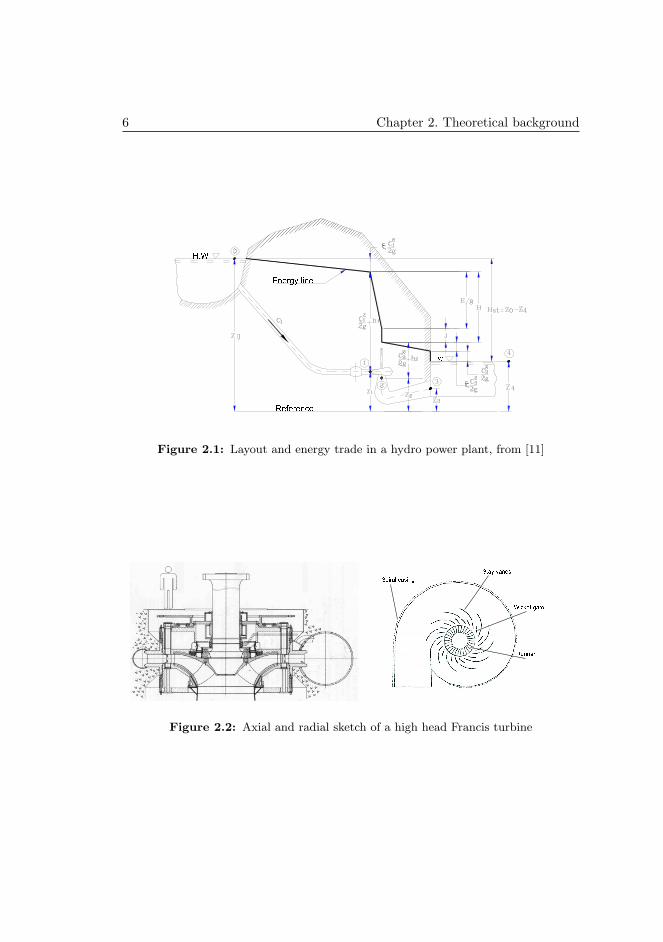
Francis turbines are usually used in power plants with heads between ca 25 to700 meter and is the most common turbine used in Norwegian power plants.A sketch of a typically high head power plant with a Francis turbine is shownin figure 2.1 on the following page, and a more detailed sketch of the differentturbine parts are shown in figure 2.2.
The wicket gate consist of a number of vanes that can be adjusted in order toincrease or reduce the flow rate through the turbine. The vanes are arrangedbetween two parallel covers normal to the turbine shaft. The main purposeof the wicket gate is to adjust the load on the turbine by regulating the flow,secondary they give the water a spin around the rotating axis before is entersthe runner.
There are some overlapping names on the wicket gate. The expression Wicketgate is often used on the whole set of guide vanes, while one or more guide vanesare simply called guide vane or guide vanes.
5
6 Chapter 2. Theoretical background
!"#
Figure 2.1: Layout and energy trade in a hydro power plant, from [11]
!#"%$'&#"!
(*)'++,%-
Figure 2.2: Axial and radial sketch of a high head Francis turbine
2.1. Francis turbine 7
The available head in a power plant is given by the difference of the high waterlevel and the tail water level and can be expressed as:
P = ρgHQ [W] (2.1)
In more detail, losses in the process must be taken into consideration. Thehydraulic efficiency of the turbine is defined as the ratio between the utilizedhead and the available head. By definition the available head is established bysubtracting the total head at the outlet of the draft tube, from the total headat the inlet of the runner. By this definition, losses in the conduit system, head-and tail race tunnels are not included in the turbine efficiency. Figure 2.1 onthe preceding page shows the power trade in a power plant, and from this figurethe expression of the available head can be obtained:
H =(
c21
2g+ h1 + z1
)−
(c23
2g+ h3 + z3
)[m] (2.2)
The hydraulic efficiency of the turbine can then be expressed as:
ηh =Hn
H[−] (2.3)
Where Hn is the net head, accounted for losses developed in the turbine anddraft tube.
At the inlet of the spiral casing, the energy is mainly pressure energy. The flowis evenly distributed around the circumference of the casing and passes the stayvanes and guide vanes before it enters the runner. Through the stay- and guidevanes the flow is accelerated, converting pressure energy to velocity energy. Atthe inlet of the runner the energy is typically 50% velocity energy and 50%pressure energy, depending on the reaction ratio of the turbine. The reactionratio is defined as the pressure drop through the runner divided on the net head,see equation (2.4).
R =h1 − h2
H[−] (2.4)
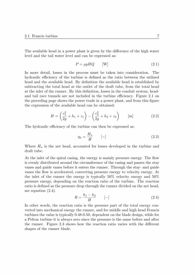
In other words, the reaction ratio is the pressure part of the total energy con-verted into mechanical energy the runner, and for middle and high head Francisturbines the value is typically 0.48-0.50, dependent on the blade design, while fora Pelton turbine it is always zero since the pressure is the same before and afterthe runner. Figure 2.3 shows how the reaction ratio varies with the differentshapes of the runner blade.
8 Chapter 2. Theoretical background
!
Figure 2.3: Runner blade shape vs. reaction ratio
! #"
$ %& '()%*+,-& ,. ,*,-/ 01 *&2,& 3-41 *,
57698 :<;=>9? @ :BADC6E:
FGIHJ K<HLMG9N O9KQPDRSDK
T7U9V W<XY[Z9U9UDW\
]^I_` a<_b ^9c9cDad
egfihj k<hlnmpoEq h9hfsrEk
tvuxwy
zs|
~
p
iD
¡¢ £ £¥¤ ¤
¦§¨©ª
Figure 2.4: Energy trade
2.2. Sources of instability 9
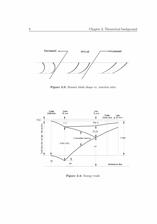
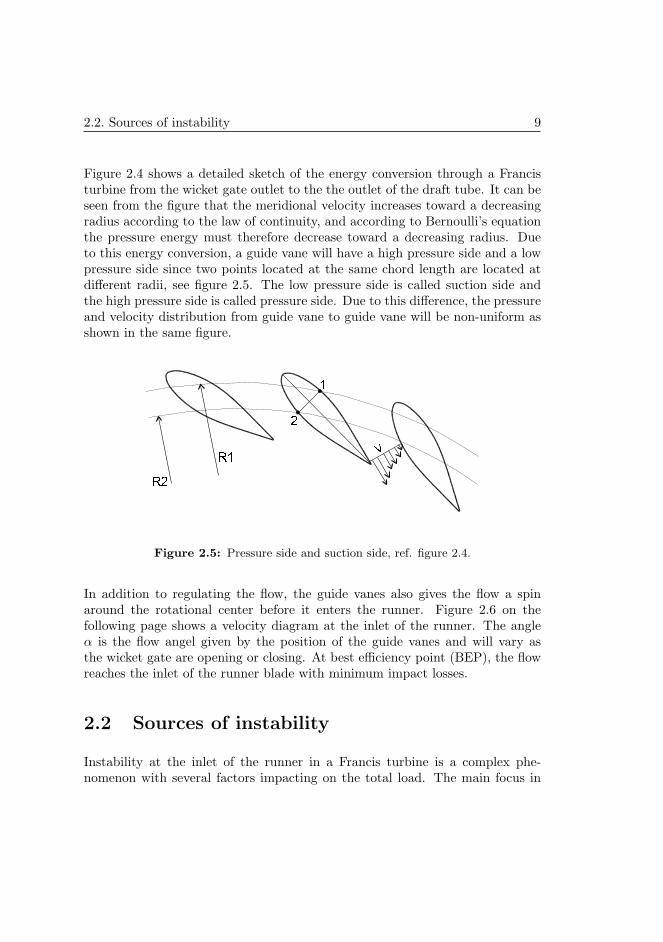
Figure 2.4 shows a detailed sketch of the energy conversion through a Francisturbine from the wicket gate outlet to the the outlet of the draft tube. It can beseen from the figure that the meridional velocity increases toward a decreasingradius according to the law of continuity, and according to Bernoulli’s equationthe pressure energy must therefore decrease toward a decreasing radius. Dueto this energy conversion, a guide vane will have a high pressure side and a lowpressure side since two points located at the same chord length are located atdifferent radii, see figure 2.5. The low pressure side is called suction side andthe high pressure side is called pressure side. Due to this difference, the pressureand velocity distribution from guide vane to guide vane will be non-uniform asshown in the same figure.
Figure 2.5: Pressure side and suction side, ref. figure 2.4.
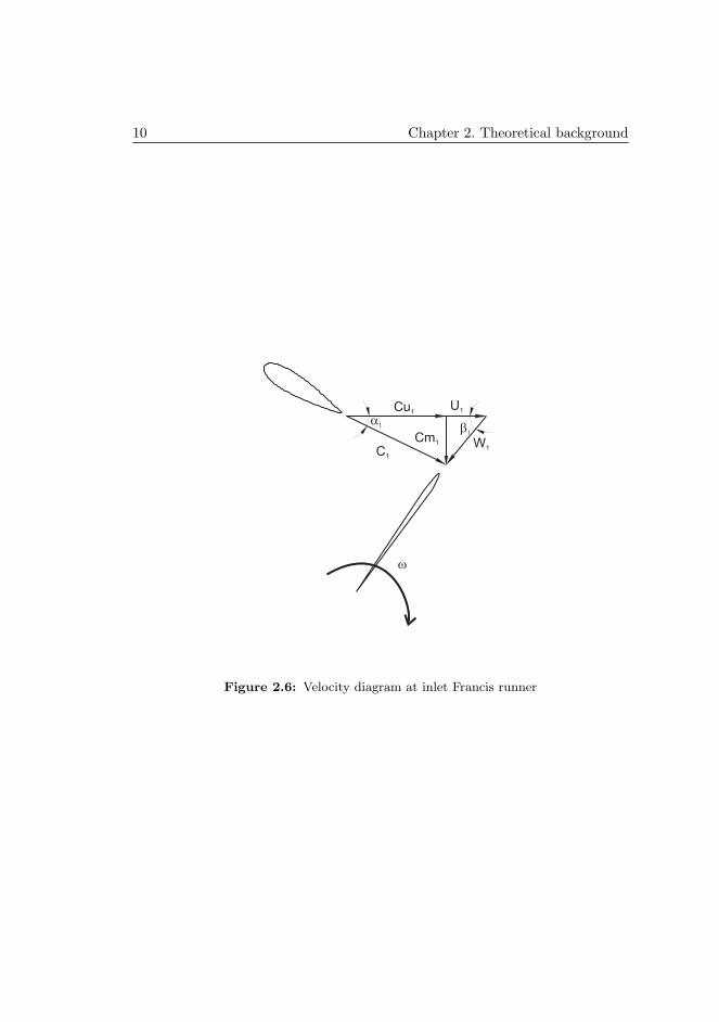
In addition to regulating the flow, the guide vanes also gives the flow a spinaround the rotational center before it enters the runner. Figure 2.6 on thefollowing page shows a velocity diagram at the inlet of the runner. The angleα is the flow angel given by the position of the guide vanes and will vary asthe wicket gate are opening or closing. At best efficiency point (BEP), the flowreaches the inlet of the runner blade with minimum impact losses.
2.2 Sources of instability
Instability at the inlet of the runner in a Francis turbine is a complex phe-nomenon with several factors impacting on the total load. The main focus in
10 Chapter 2. Theoretical background
U1
W1
C1
Cu1
Cm1
Figure 2.6: Velocity diagram at inlet Francis runner
2.2. Sources of instability 11
this thesis has been on the interaction between the wicket gate and the runner.However, some of the most common sources of instability will also be shortlydescribed in the following. For further study on the different topics, it is referredto the textbook by Brennen [13] or PhD-thesis by e.g Stepanik [63], Jernsletten[32], Vekve [68] and Larsson [40].
There are different phenomena that can cause vibrations and pressure pulsesthrough the turbine, some due to the mechanical design and some due to thelocal condition of the flow. A short outline of the most common sources ofvibration and pressure pulses will be given, followed by a review of previouswork within the topics with emphasize on pressure pulses at the inlet of therunner. Factors that are important for this thesis’ topic will be handled morethorough in section 2.4 on page 15.
The stay vanes might cause vibration due to vortex shedding of von Karmanvortices. These vortices have a distinct frequency which can be calculated withthe Strouhal formula and empirical values. If this frequencies are in the samerange as the natural frequency of the stay vanes, resonance may cause severevibrations and cracking at the stay vane. The stay vane will also cause a wakewhich disturbs the flow at the inlet of the guide vanes. Most of the effects causedby the stay vanes will, however, be dampened out before they reach the runner.
Due to their slim profile and thin trailing edge, vortex shedding from the guidevanes will have high frequency and low amplitude, according to [2], and willseldom cause severe problems as long as resonance frequencies are avoided. Themain influence from the guide vanes are the viscous wake and the creation ofa non uniform flow field in which the runner blades will rotate. As it will bedescribed in the following sections, the severity of this phenomenon is highlydependent of several design parameters. The number of wicket gates and thedesign of them, the number of runner blades and the distance between thewicket gate and runner are some of the most important parameters and will bedescribed in more details in the following sections.
In the runner, stall may occur if the flow have large angles of incidence to theblades. The large incidence angle causes a local eddy at one blade, blocking themain flow and impact on the incidence angle of the nearby blades. Hence thestall will rotate around the runner, so called rotating stall. Stall is very rare inFrancis turbines, it is normally found in centrifugal pumps, and pump turbines.The frequency of the rotating stall cell is typically 0.5-0.7 times the rotationalfrequency of the runner or impeller.
12 Chapter 2. Theoretical background
Hydraulic deviations in the waterways or spiral casing can induce a netradial force on the runner. This force can cause a displacement of the runnerand produce pressure pulses with a frequency equal to the rotational frequencyof the runner [40], [64].
In the draft tube cone and draft tube, surge is the main source of pressurepulsations. At off-design conditions swirl flow from the runner will cause varyingpressure in the draft tube cone. At part load, this swirl has a shape of a rotatingrope, rotating in the same direction as the runner. The frequency of the rotationis the so called Rheingans frequency, approximately 1/3 of the rotational speedof the runner. At full load, the swirl rotates in the opposite direction of therunner and has the shape of a axi-symmetric cavity.
Turbulence and cavitation excites a broad band of frequencies with ran-domly variation, and will therefore not induce any pressure pulses at a certainfrequency. Cavitation can, however, under certain condition indirectly causepressure pulses through a phenomenon called ”partial cavitation oscillation.”This is more thoroughly described by e.g Brennen, [13, Chapter 8].
2.3 Previous work
A review of previous work within this fields will be presented in following sec-tions. Textbooks within the topic of turbine vibrations are rare, however thereare some books for pumps which covers most of the same phenomenons. Bren-nen’s [13] book covers hydrodynamics of pumps and most of the topics are validfor turbines as well.
There has been quite a lot of PhD work on this topic. One of them is Lund[46] who described the propagation of the pressure pulses in the volute regionbetween the guide vanes and runner by means of Fourier series. With a mathe-matically expression of the wave propagations, favorable and unfavorable com-binations of number of guide vanes and runner vanes have been calculated.
Stepanik [63] focused on improved part load performance in pump turbines. Byincreasing the number of impeller blades from seven to nine and increasing theblade curvature, part load performances in both pump-mode and turbine-modehave been increased due to more uniform load on the impeller blades. This alsocaused a reduction of the unsteady pressure fluctuations in the runner.
2.3. Previous work 13
Jernsletten [32] measured pressure pulses in a model of a Francis turbinerunner. Measurements were carried out with pressure transducers on the runnerblades, and the results showed a 30% reduction of the pressure pulses on therunner when the distance between the guide vanes and the runner was increasedby 5.1 mm.
Larsson [40] investigated the flow field at the inlet of the runner of a Francisturbine in detail. The thesis presented a detailed research of the unsteady inletflow of a high head Francis pump turbine. The inlet flow field was measured withLDA and pressure pulses between the guide vanes and runner were measured.The results showed that the flow rate in a guide vane passage fluctuates up to15% of the mean flow due to the influence of the runner blade passages. Boththe pressure pulses and the velocity field distinctly changed character whenthe rotational speed was increased 20 % above the best efficiency point. Themeasurements also showed that the viscous wake was completely attenuated atthe inlet of the runner. Which means that for this turbine, the non-uniform flowfield was set up by accelerated flow through the stay and guide vane passage.CFD calculations showed good agreement with the stationary stay and guidevane flow while unsteady calculations, including the runner, deviated somewhatfrom the measurements.
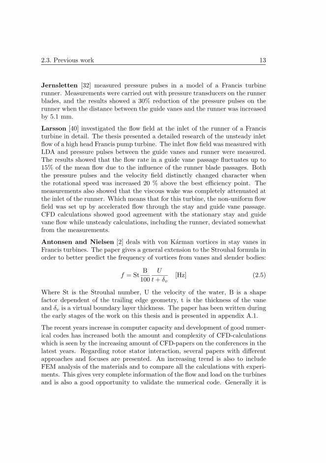
Antonsen and Nielsen [2] deals with von Karman vortices in stay vanes inFrancis turbines. The paper gives a general extension to the Strouhal formula inorder to better predict the frequency of vortices from vanes and slender bodies:
f = StB
100U
t + δv[Hz] (2.5)
Where St is the Strouhal number, U the velocity of the water, B is a shapefactor dependent of the trailing edge geometry, t is the thickness of the vaneand δv is a virtual boundary layer thickness. The paper has been written duringthe early stages of the work on this thesis and is presented in appendix A.1.
The recent years increase in computer capacity and development of good numer-ical codes has increased both the amount and complexity of CFD-calculationswhich is seen by the increasing amount of CFD-papers on the conferences in thelatest years. Regarding rotor stator interaction, several papers with differentapproaches and focuses are presented. An increasing trend is also to includeFEM analysis of the materials and to compare all the calculations with experi-ments. This gives very complete information of the flow and load on the turbinesand is also a good opportunity to validate the numerical code. Generally it is
14 Chapter 2. Theoretical background
quite good agreement between calculations and experiments, given that enougheffort is made in order to create a fine enough mesh and take the cost of longcalculation time.
Ruprecht et al [59] carried out a numerical calculations of a complete Francisturbine, including spiral case, stay vanes, guide vanes, runner and draft tube.The motivation for this was to avoid simplifications and periodic assumptions.This resulted in a huge mesh size and very costly in terms of computer time.
Also Page et al [54] compute transient rotor stator interaction by modeling thewhole turbine from spiral case to draft tube. The use of large eddy simulation(LES), gave quite good results compared with experiments.
Segoufin et al [61] did a comprehensive analysis of unsteadiness in a high headpump turbine. Calculations including a 3D-model of the whole runner, wicketgate and stay vanes were carried out together with a simplified 2D calculation.Calculating the fluctuations at the guide vanes and runner blades, the resultsshowed that the 2D calculations only varied about 6% from the 3D calculationswhich opens for a tremendous saving in computational time, using 2D insteadof 3D. While a complete 3D calculation require CPU-time in means of weeks,the 2D calculations can be carried out in hours.
An interesting fact, presented by Zobeiri et al [79] shows that the pressureactually will fluctuate all the way upstream the stay vanes due to the passingof a runner blade. This is in agreement with the measurements carried out byLarsson [40].
Even though a calculation of the whole turbine geometry gives valuable infor-mation, the time aspect makes this kind of calculations poor fitted for industrialuse. A paper presented by Nennemann et al [48] describes how GE Energyuses CFD in turbine design. By comparing numerical calculations with exper-iments, a way to simplify the calculations was found. If the ratio between thearea of stationary and rotating interfaces lies between 0.99-1.01, the simplifica-tion gives negligible impact on the results. For example a case with 24 guidevanes and 17 runner blades can be reduced to 7 wicket gates and 5 runner bladeswith an area ratio of 0.99167. This will significantly reduce the mesh size andsave calculation time.
As it just have been shown; lots of work have been carried out in order toinvestigate the interaction between the wicket gate and the runner. The flowfield is complex and highly time dependent. Also the design of each turbine willaffect the flow, since a pump turbine with, say, 8 runner blades will have quite
2.4. Wake flow 15
a different ’interaction pattern’ than a high head turbine with, say, 24 runnerblades (including splitter blades). This makes it difficult to draw out generalguide lines to cover all different cases. Some rules of thumb are acknowledgedas important and general guide lines, e.g the ratio between the number of guidevanes and runner blades, and the distance between the outlet of the guide vanesand inlet of the runner blades. However, the design of the guide vanes in orderto reduce the dynamic load on the runner is seldom discussed. In the followingsections the rotor/stator interaction phenomena will be presented in more detailand also how the design of the wicket gate can contribute to reduce the dynamicload on the runner. The presented hypothesis are based upon fundamental fluidtheory, and a short introduction of topics of current interest will be given.
2.4 Wake flow
The first approaches to the theory of fluid dynamics assumed perfect, frictionlessfluid behavior. Euler developed both the differential equations of motion andtheir integrated form, now called the Bernoulli equation. D’ Alembert used theseequations to show his famous paradox; that a body immersed in a frictionlessflow has zero drag. After Navier and Stokes successfully added the viscous termsto the equations of motion and Prandtl introduced the boundary layer theory,calculations on real flow could be carried out [74].
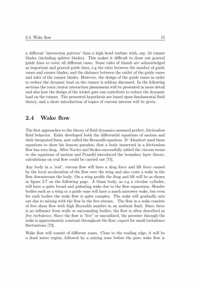
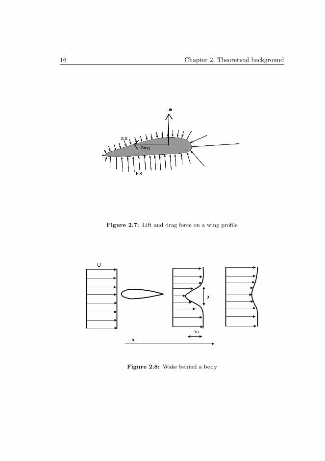
Any body in a ’real’, viscous flow will have a drag force and lift force causedby the local acceleration of the flow over the wing and also crate a wake in theflow downstream the body. On a wing profile the drag and lift will be as shownin figure 2.7 on the following page. A blunt body, as e.g a circular cylinder,will have a quite broad and pulsating wake due to the flow separation. Slenderbodies such as a wing or a guide vane will have a much narrower wake, but evenfor such bodies the wake flow is quite complex. The wake will gradually mixout due to mixing with the flow in the free stream. The flow in a wake consistsof free shear flow with high Reynolds number in an ambient fluid. Since thereis no influence from walls or surrounding bodies, the flow is often described asfree turbulence. Since the flow is ”free” or unconfined, the pressure through thewake is approximately constant throughout the flow, expect for small turbulencefluctuations [73].
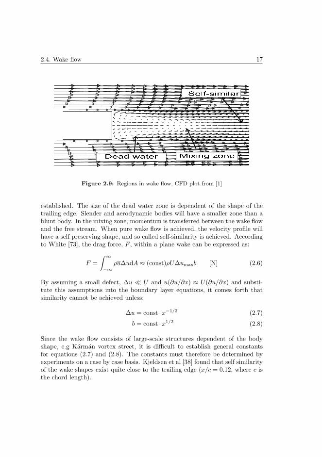
Wake flow will consist of different zones. Close to the trailing edge, it will bea dead water region, followed by a mixing zone before the pure wake flow is
16 Chapter 2. Theoretical background
Figure 2.7: Lift and drag force on a wing profile
Figure 2.8: Wake behind a body
2.4. Wake flow 17
"!$#% &% '(
Figure 2.9: Regions in wake flow, CFD plot from [1]
established. The size of the dead water zone is dependent of the shape of thetrailing edge. Slender and aerodynamic bodies will have a smaller zone than ablunt body. In the mixing zone, momentum is transferred between the wake flowand the free stream. When pure wake flow is achieved, the velocity profile willhave a self preserving shape, and so called self-similarity is achieved. Accordingto White [73], the drag force, F , within a plane wake can be expressed as:
F =∫ ∞
−∞ρu∆udA ≈ (const)ρU∆umaxb [N] (2.6)
By assuming a small defect, ∆u U and u(∂u/∂x) ≈ U(∂u/∂x) and substi-tute this assumptions into the boundary layer equations, it comes forth thatsimilarity cannot be achieved unless:
∆u = const ·x−1/2 (2.7)
b = const ·x1/2 (2.8)
Since the wake flow consists of large-scale structures dependent of the bodyshape, e.g Karman vortex street, it is difficult to establish general constantsfor equations (2.7) and (2.8). The constants must therefore be determined byexperiments on a case by case basis. Kjeldsen et al [38] found that self similarityof the wake shapes exist quite close to the trailing edge (x/c = 0.12, where c isthe chord length).
18 Chapter 2. Theoretical background
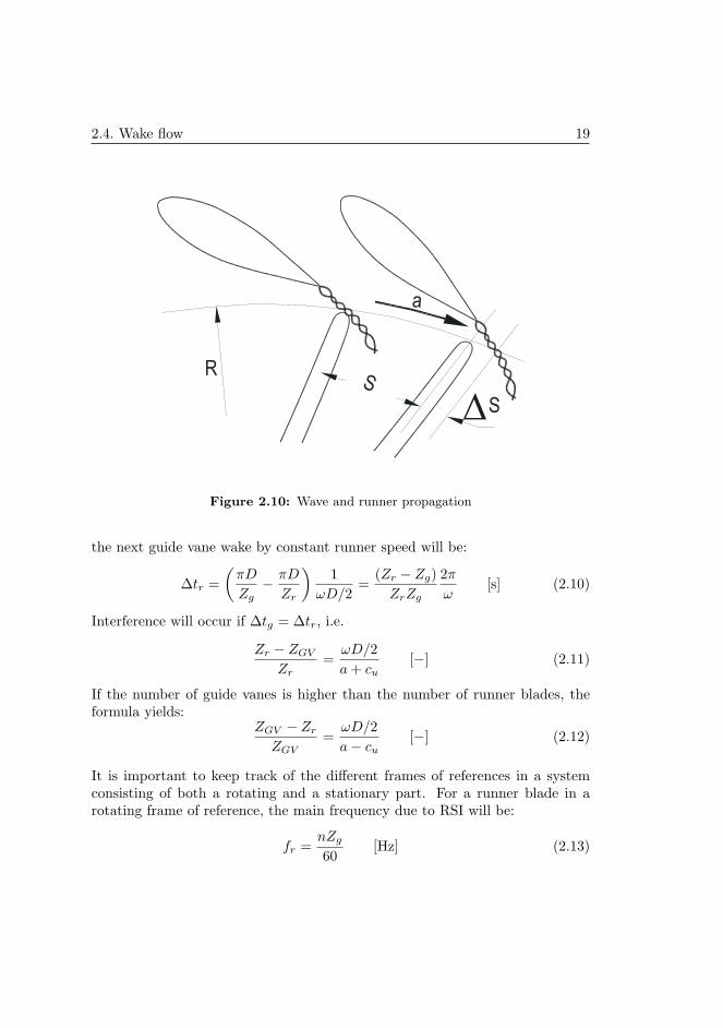
As the previous pages concluded, the flow field downstream the wicket gateconsists of a blade-to-blade pressure difference, both due to the accelerated flowfield and the local pressure and suction side of the vanes. In addition, theviscous wake will create a velocity defect, affecting the velocity distribution.The runner blades will also have a blade-to-blade pressure difference and due tothe rotation of the runner, this pressure difference will rotate with the runner.In addition to this, the stagnation point at the leading edge of the runner bladeswill also rotate with the runner. Every pressure wave created will travel aroundthe circumference with the speed of sound until it is dampened out. Togetherthis will cause a complicated pressure field in the region between the outletof the wicket gate and inlet of the runner. However, the pressure propagationcan be described by means of Fourier series e.g as suggested by Nicolet et al.[50] or Lund [46]. A far more easy and strait forward approach can be used tovisualize the phenomenon: Imagine a pressure pulse created each time a runnerblade passing a guide vane, traveling around the circumference with the speedof sound. Amplifications of the pressure pulses may occur if the combinationof number of guide vanes and number of runner blades is unfavorable. If thenumber of guide vanes and runner blades have a common factor, more than oneblade will hit a wake at the same time. With e.g. 24 guide vanes and 30 runnerblades, 6 runner blades are passing 6 guide vanes simultaneously while 5 bladesin front of each blade are passing wakes before the regarded blade is passing thenext guide vane wake. As a result, 5 pressure pulsations are entering the runnerin-between each blade passing frequency of a regarding blade.
Amplification may also occur if the shock propagation speed from one bladepassing pulse reaches the next guide vane wake at the same time as the bladein front of the regarding blade is passing the wake. This situation occur if thenumber of runner blades is higher than the number of guide vanes. If the numberof guide vanes is higher than the number of runner blades, the shock wave willtravel in the opposite direction.
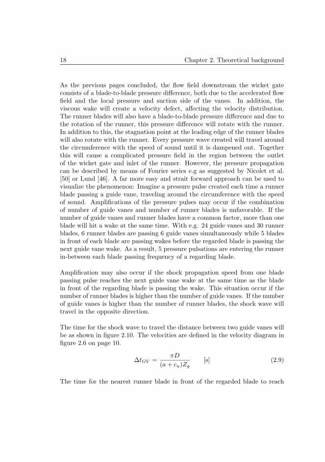
The time for the shock wave to travel the distance between two guide vanes willbe as shown in figure 2.10. The velocities are defined in the velocity diagram infigure 2.6 on page 10.
∆tGV =πD
(a + cu)Zg[s] (2.9)
The time for the nearest runner blade in front of the regarded blade to reach
2.4. Wake flow 19
RS
S
a
Figure 2.10: Wave and runner propagation
the next guide vane wake by constant runner speed will be:
∆tr =(
πD
Zg− πD
Zr
)1
ωD/2=
(Zr − Zg)ZrZg
2π
ω[s] (2.10)
Interference will occur if ∆tg = ∆tr, i.e.
Zr − ZGV
Zr=
ωD/2a + cu
[−] (2.11)
If the number of guide vanes is higher than the number of runner blades, theformula yields:
ZGV − Zr
ZGV=
ωD/2a− cu
[−] (2.12)
It is important to keep track of the different frames of references in a systemconsisting of both a rotating and a stationary part. For a runner blade in arotating frame of reference, the main frequency due to RSI will be:
fr =nZg
60[Hz] (2.13)

20 Chapter 2. Theoretical background
For a stationary point, the corresponding frequency will be:
fGV =nZr
60[Hz] (2.14)

Chapter 3
Numerical model
In order to test the hypothesis, a series of CFD-calculations have been carriedout. Pressure distribution downstream guide vanes with different profiling havebeen calculated and compared. Also the velocity defect in the wakes has beencalculated as a factor suitable for comparison with experimental data. Thecommercial program Fluent 6.2.16 with Gambit 2.2.30 as a preprocessor hasbeen used for all the calculations.
3.1 Model details
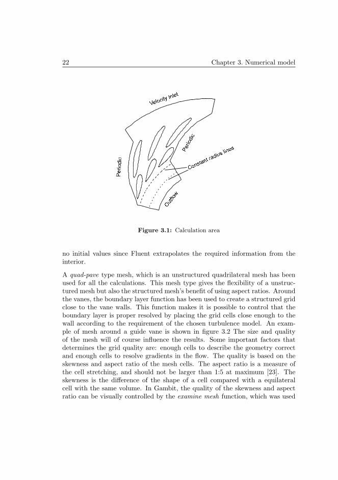
According to experience, it has been assumed that a simplified model consistingof three stay vanes and three guide vanes in a periodic, 2-dimensional domainwould be sufficient for this kind of calculations. The calculation area is shown infigure 3.1 on the following page. The inlet was located a chord length upstreamthe stay vanes in order to let the flow field to be fully developed at the inlet ofthe stay vanes. The outlet was located a chord length downstream the point ofwhere the inlet of the runner would be. Inlet boundary condition was velocityinlet, set as velocity components in x and y direction. The inlet velocity wasequal to the velocity used in the experiment, see chapter 4 on page 33, and theflow angle was set to match the inlet angle of the stay vanes and guide vanes.Outflow boundary condition has been used at the outlet. This condition requires
21
22 Chapter 3. Numerical model
"!$#% &(' )
*,+-/.1032 - 054 2687 9 .;:
7 -=< .
Figure 3.1: Calculation area
no initial values since Fluent extrapolates the required information from theinterior.
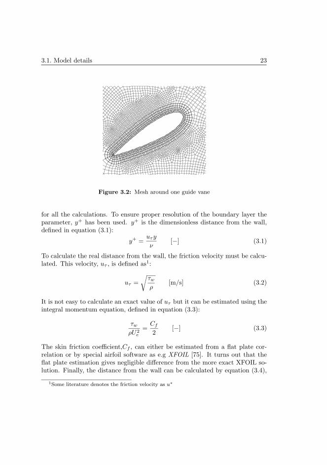
A quad-pave type mesh, which is an unstructured quadrilateral mesh has beenused for all the calculations. This mesh type gives the flexibility of a unstruc-tured mesh but also the structured mesh’s benefit of using aspect ratios. Aroundthe vanes, the boundary layer function has been used to create a structured gridclose to the vane walls. This function makes it is possible to control that theboundary layer is proper resolved by placing the grid cells close enough to thewall according to the requirement of the chosen turbulence model. An exam-ple of mesh around a guide vane is shown in figure 3.2 The size and qualityof the mesh will of course influence the results. Some important factors thatdetermines the grid quality are: enough cells to describe the geometry correctand enough cells to resolve gradients in the flow. The quality is based on theskewness and aspect ratio of the mesh cells. The aspect ratio is a measure ofthe cell stretching, and should not be larger than 1:5 at maximum [23]. Theskewness is the difference of the shape of a cell compared with a equilateralcell with the same volume. In Gambit, the quality of the skewness and aspectratio can be visually controlled by the examine mesh function, which was used
3.1. Model details 23
Figure 3.2: Mesh around one guide vane
for all the calculations. To ensure proper resolution of the boundary layer theparameter, y+ has been used. y+ is the dimensionless distance from the wall,defined in equation (3.1):
y+ =uτy
ν[−] (3.1)
To calculate the real distance from the wall, the friction velocity must be calcu-lated. This velocity, uτ , is defined as1:
uτ =√
τw
ρ[m/s] (3.2)
It is not easy to calculate an exact value of uτ but it can be estimated using theintegral momentum equation, defined in equation (3.3):
τw
ρU2e
=Cf
2[−] (3.3)
The skin friction coefficient,Cf , can either be estimated from a flat plate cor-relation or by special airfoil software as e.g XFOIL [75]. It turns out that theflat plate estimation gives negligible difference from the more exact XFOIL so-lution. Finally, the distance from the wall can be calculated by equation (3.4),
1Some literature denotes the friction velocity as u∗
24 Chapter 3. Numerical model
by estimating the skin friction coefficient and choosing an appropriate value ofy+:
y =y+ν
uτ=
y+ν√Cf U2
∞2
[m] (3.4)
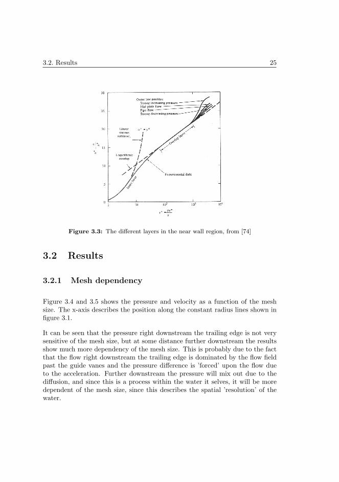
The importance of creating the mesh at correct distance from the wall is dueto the wall and the boundary layer’s influence on the turbulent flow. Both thephysical wall and the boundary layer, in which the viscous forces are dominant,will dampen out the turbulent fluctuations. The turbulence models are onlyvalid in ’free stream turbulent flow’. Figure 3.3 on the facing page shows thethree layers of the flow; the viscous inner layer, the overlap layer and the outerlayer, in which the wall law is valid. To ensure that the boundary layer isproperly resolved, the y+ value is set according to the recommended values inthe Fluent manual [23], and as shown in figure 3.3, between 30-300, dependentof the mesh size and choice of turbulence model.
In Fluent, there are two different approaches to modeling the two inner re-gions. Either by wall functions or near wall modeling. The wall function usessemi-empirical formulas as a ’bridge’ between the two inner layers and the fullyturbulent region. The near wall approach modifies the turbulence models to bevalid all the way down to the wall. If this approach is used, the mesh must becreated with y+ < 5.
The meshing strategy was first to calculate an appropriate distance from thewall to place the first mesh cell, thereafter a mesh was generated accordingto experience and the guidelines from the Fluent manual. The mesh was thenrefined until the results from the calculations did not change. Then the mesh wascoarsened as much as possible until the results was changed. By this iterationit was ensured that a mesh-independent solution was found and still reduce themesh size, and hence the computer time, as much as possible.
The calculations were considered converged when the residuals reached a con-stant value. According to the Fluent manual [23], a residual value of 10−3 issufficient and for standard computers, any value below 10−5 will be roundingerrors in the computer system. The convergence of lift and drag force is alsoused to determine the convergence, together with the mass balance between in-let and outlet. The mass flow is calculated at inlet and outlet and should beequal if the calculations are perfectly correct. Large differences in the mass flowindicates numerical inaccuracy, but in all cases the differences were in a orderof magnitude of 10−5, which indicates an accurate solution.
3.2. Results 25
Figure 3.3: The different layers in the near wall region, from [74]
3.2 Results
3.2.1 Mesh dependency
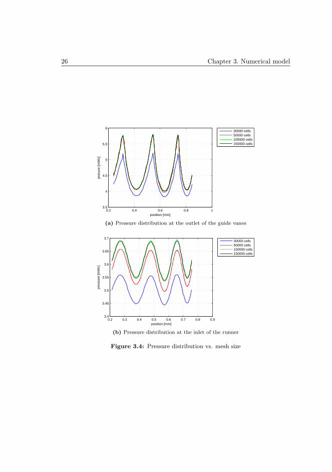
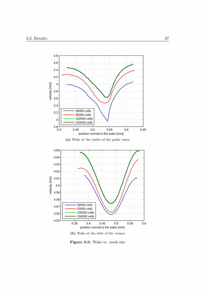
Figure 3.4 and 3.5 shows the pressure and velocity as a function of the meshsize. The x-axis describes the position along the constant radius lines shown infigure 3.1.
It can be seen that the pressure right downstream the trailing edge is not verysensitive of the mesh size, but at some distance further downstream the resultsshow much more dependency of the mesh size. This is probably due to the factthat the flow right downstream the trailing edge is dominated by the flow fieldpast the guide vanes and the pressure difference is ’forced’ upon the flow dueto the acceleration. Further downstream the pressure will mix out due to thediffusion, and since this is a process within the water it selves, it will be moredependent of the mesh size, since this describes the spatial ’resolution’ of thewater.
26 Chapter 3. Numerical model
0.2 0.4 0.6 0.8 13.5
4
4.5
5
5.5
6
position [mm]
pres
ure
[mW
c]
30000 cells50000 cells100000 cells150000 cells
(a) Pressure distribution at the outlet of the guide vanes
0.2 0.3 0.4 0.5 0.6 0.7 0.8 0.93.4
3.45
3.5
3.55
3.6
3.65
3.7
position [mm]
pres
sure
[mW
c]
30000 cells50000 cells100000 cells150000 cells
(b) Pressure distribution at the inlet of the runner
Figure 3.4: Pressure distribution vs. mesh size
3.2. Results 27
0.4 0.45 0.5 0.55 0.6 0.652.8
3
3.2
3.4
3.6
3.8
4
4.2
4.4
4.6
4.8
position normal to the wake [mm]
velo
city
[m/s
]
30000 cells50000 cells100000 cells150000 cells
(a) Wake at the outlet of the guide vanes
0.35 0.4 0.45 0.5 0.55 0.64.55
4.56
4.57
4.58
4.59
4.6
4.61
4.62
4.63
4.64
4.65
position normal to the wake [mm]
velo
city
[m/s
]
30000 cells50000 cells100000 cells150000 cells
(b) Wake at the inlet of the runner
Figure 3.5: Wake vs. mesh size
28 Chapter 3. Numerical model
3.2.2 Turbulence model dependency
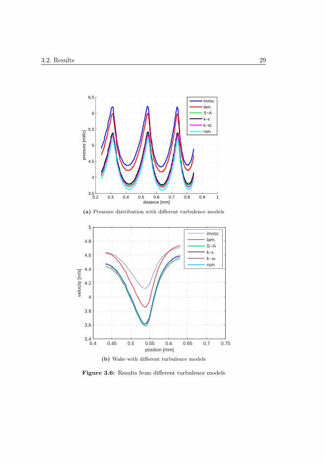
The k − ε turbulence model has been used since this is the simplest of the’complete models’ and, hence, the less costly in terms of computational time.The model assumes that the flow is fully turbulent and that the effect of themolecular viscosity is negligible. The model is well known and well developed,with good accuracy for a wide range of turbulent flows. The standard modelhas been improved as its weaknesses has been derived throughout the years. InFluent, two variants of the standard model is available: The RNG-model andthe realizable-model. The standard model has been used in this thesis. Forcomparison, the different models in Fluent have been used. Especially the one-equation model, Spalart-Allmaras, is of interest since this model was designedspecifically for the wing profiles and aerospace applications and are built to usemeshes that resolve the viscous regions. This means that the model should havea mesh similar to the k − ε model with enhanced wall treatment. Being a one-equation model the calculation time will be shorter than for the two-equationk − ε model. Figure 3.6 show the pressure distribution and the velocity wakefor calculations with different turbulence models.
As the figure shows, there are small differences between the different turbulencemodels, while the laminar and inviscid solutions differ from the other solutions.As expected, these models show a less dampened flow and a flow with less lossesthan the turbulent cases. It can also be seen that the pressure distribution is notvery dependent on the viscosity, since even the inviscous solution shows a distinctvariation in the pressure. Naturally, there are relatively larger differences in thewake since this is more dependent of the viscosity.
3.2.3 Pressure distribution
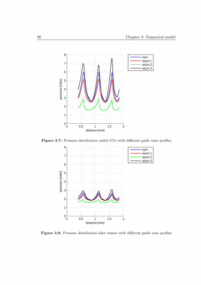
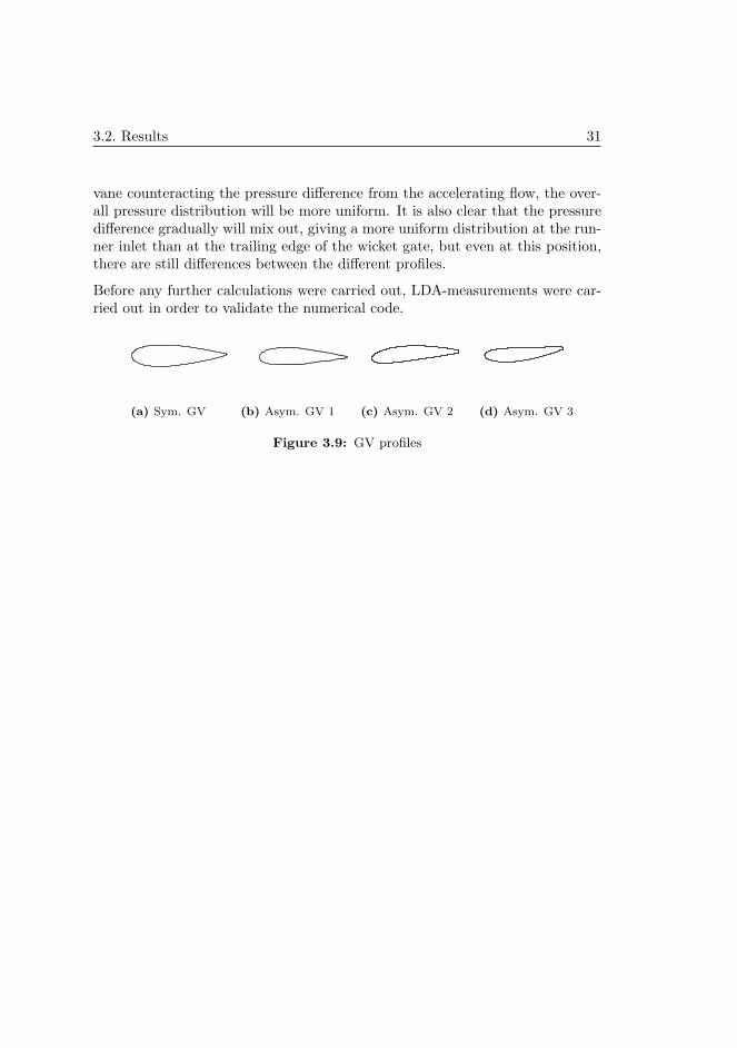
Four different guide vane profiles have been calculated in order to see what in-fluence the profile has on the pressure distribution. One symmetric, one slightlyasymmetric the ’correct’ way (’flat side’ toward the runner), and two moreextreme asymmetric profiles, both on the ’correct’ side and ’wrong’ side, see fig-ure 3.9 on page 31. The pressure distribution at the outlet of the guide vanes forthe different profiles is shown in figure 3.7 on page 30 and figure 3.8 on page 30shows the pressure distribution at the inlet of the runner.
It is clear that the profiling of the guide vanes does impact the pressure dis-tribution, according to the hypothesis. With the pressure side of the guide
3.2. Results 29
0.2 0.3 0.4 0.5 0.6 0.7 0.8 0.9 13.5
4
4.5
5
5.5
6
6.5
distance [mm]
pres
sure
[mW
c]
invisc.lam.S−A
k−εk−ωrsm
(a) Pressure distribution with different turbulence models
0.4 0.45 0.5 0.55 0.6 0.65 0.7 0.753.4
3.6
3.8
4
4.2
4.4
4.6
4.8
5
position [mm]
velo
city
[m/s
]
invisc.lam.S−Ak−εk−ωrsm
(b) Wake with different turbulence models
Figure 3.6: Results from different turbulence models
30 Chapter 3. Numerical model
0 0.5 1 1.5 20
1
2
3
4
5
6
7
8
distance [mm]
pres
sure
[mW
c]
sym.asym.1asym.2asym.3
Figure 3.7: Pressure distribution outlet GVs with different guide vane profiles
0 0.5 1 1.5 20
1
2
3
4
5
6
7
8
distance [mm]
pres
sure
[mW
c]
sym.asym.1asym.2asym.3
Figure 3.8: Pressure distribution inlet runner with different guide vane profiles
3.2. Results 31
vane counteracting the pressure difference from the accelerating flow, the over-all pressure distribution will be more uniform. It is also clear that the pressuredifference gradually will mix out, giving a more uniform distribution at the run-ner inlet than at the trailing edge of the wicket gate, but even at this position,there are still differences between the different profiles.
Before any further calculations were carried out, LDA-measurements were car-ried out in order to validate the numerical code.
(a) Sym. GV (b) Asym. GV 1 (c) Asym. GV 2 (d) Asym. GV 3
Figure 3.9: GV profiles

32 Chapter 3. Numerical model

Chapter 4
Experiment
In order to verify the CFD-calculations and gain more information for this kindof flow field, a measurement series has been carried out. This chapter willpresent the setup for the test rigs, describe the different techniques and detailsabout the equipment. The velocity distribution in the wake downstream theguide vanes have been measured using the LDA-technique, while hollow guidevanes have made it possible to measure the pressure distribution around theguide vane profile with a pressure transducer. The results have been used as acomparison to the CFD-calculation, and will be presented in section 4.2.
A test series with dynamic pressure pulse measurements in a Francis modelturbine has also been carried out. Pressure transducers mounted in the lowercover in the volute region between the outlet of the wicket gate and the inlet ofthe runner have been used in order to measure the fluctuating pressure. Sincethis measures the load on the wicket gate from the runner, and not the load onthe runner from the wicket gate, this measurements are omitted from the mainpart of this thesis and are presented in appendix A.3, as a paper submitted tothe 23th IAHR symposium.
33
34 Chapter 4. Experiment
4.1 Experimental set-up
4.1.1 LDA principles and rig setup
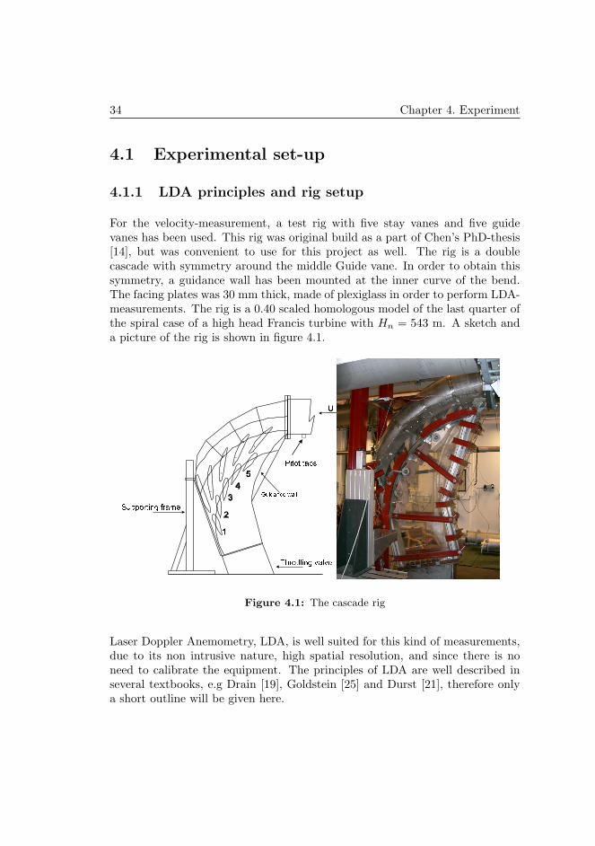
For the velocity-measurement, a test rig with five stay vanes and five guidevanes has been used. This rig was original build as a part of Chen’s PhD-thesis[14], but was convenient to use for this project as well. The rig is a doublecascade with symmetry around the middle Guide vane. In order to obtain thissymmetry, a guidance wall has been mounted at the inner curve of the bend.The facing plates was 30 mm thick, made of plexiglass in order to perform LDA-measurements. The rig is a 0.40 scaled homologous model of the last quarter ofthe spiral case of a high head Francis turbine with Hn = 543 m. A sketch anda picture of the rig is shown in figure 4.1.
! #"$ %'&()%'*
+-,/..013254768 9:1<;= >
?A@CBEDCFHGJILKNM/FPOQO
Figure 4.1: The cascade rig
Laser Doppler Anemometry, LDA, is well suited for this kind of measurements,due to its non intrusive nature, high spatial resolution, and since there is noneed to calibrate the equipment. The principles of LDA are well described inseveral textbooks, e.g Drain [19], Goldstein [25] and Durst [21], therefore onlya short outline will be given here.
4.1. Experimental set-up 35
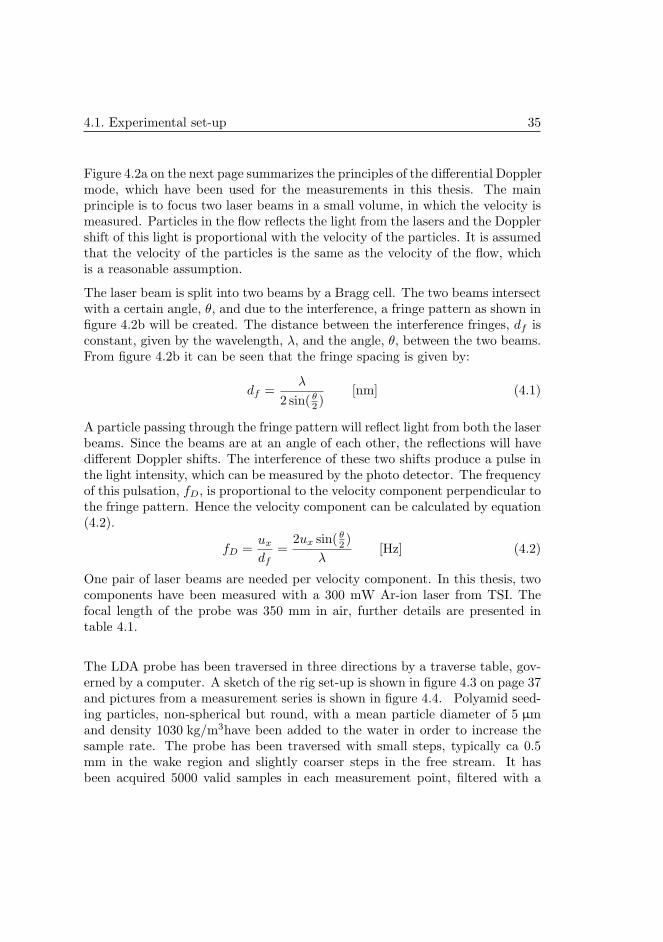
Figure 4.2a on the next page summarizes the principles of the differential Dopplermode, which have been used for the measurements in this thesis. The mainprinciple is to focus two laser beams in a small volume, in which the velocity ismeasured. Particles in the flow reflects the light from the lasers and the Dopplershift of this light is proportional with the velocity of the particles. It is assumedthat the velocity of the particles is the same as the velocity of the flow, whichis a reasonable assumption.
The laser beam is split into two beams by a Bragg cell. The two beams intersectwith a certain angle, θ, and due to the interference, a fringe pattern as shown infigure 4.2b will be created. The distance between the interference fringes, df isconstant, given by the wavelength, λ, and the angle, θ, between the two beams.From figure 4.2b it can be seen that the fringe spacing is given by:
df =λ
2 sin( θ2 )
[nm] (4.1)
A particle passing through the fringe pattern will reflect light from both the laserbeams. Since the beams are at an angle of each other, the reflections will havedifferent Doppler shifts. The interference of these two shifts produce a pulse inthe light intensity, which can be measured by the photo detector. The frequencyof this pulsation, fD, is proportional to the velocity component perpendicular tothe fringe pattern. Hence the velocity component can be calculated by equation(4.2).
fD =ux
df=
2ux sin( θ2 )
λ[Hz] (4.2)
One pair of laser beams are needed per velocity component. In this thesis, twocomponents have been measured with a 300 mW Ar-ion laser from TSI. Thefocal length of the probe was 350 mm in air, further details are presented intable 4.1.
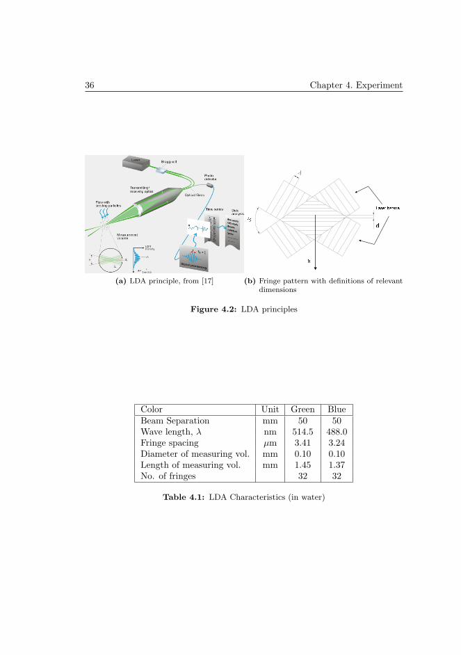
The LDA probe has been traversed in three directions by a traverse table, gov-erned by a computer. A sketch of the rig set-up is shown in figure 4.3 on page 37and pictures from a measurement series is shown in figure 4.4. Polyamid seed-ing particles, non-spherical but round, with a mean particle diameter of 5 µmand density 1030 kg/m3have been added to the water in order to increase thesample rate. The probe has been traversed with small steps, typically ca 0.5mm in the wake region and slightly coarser steps in the free stream. It hasbeen acquired 5000 valid samples in each measurement point, filtered with a
36 Chapter 4. Experiment
(a) LDA principle, from [17]
(b) Fringe pattern with definitions of relevantdimensions
Figure 4.2: LDA principles
Color Unit Green BlueBeam Separation mm 50 50Wave length, λ nm 514.5 488.0Fringe spacing µm 3.41 3.24Diameter of measuring vol. mm 0.10 0.10Length of measuring vol. mm 1.45 1.37No. of fringes 32 32
Table 4.1: LDA Characteristics (in water)
4.1. Experimental set-up 37
! " ! # $&%' (*),+.-/021 3456*5456 789:
;<=?>&@BA CD
Figure 4.3: LDA set-up
Figure 4.4: LDA measurements

38 Chapter 4. Experiment
coincidence window which means that the software only accept signals whenthe two components are measured simultaneously within a given time window.According to the TSI-manuals [66], this window have been set to the inverse ofthe sample rate, typically 104 ms for most of the measurements.
The Find software provided a post processing routine from which the mean ve-locity, variance and turbulence intensity have been calculated using the followingformulas:
u =1N
N∑i=1
ui (4.3)
σ2 =1N
N∑i=1
(ui − u)2 (4.4)
Tu =σ
u· 100% (4.5)
Where N is the number of valid samples. The following parameters have beenvaried during the tests:
• Two different guide vane profiles
• Two different guide vane angles, α
• Three different flow rates, Q
• Different downstream positions
• Different span-wise positions
(a) Symmetric profile (b) Asymmetric profile
Figure 4.5: Guide vane profiles
The profile of the two guide vanes is shown in figure 4.5. The guide vane infigure 4.5a is a symmetric profile with chord length 335 mm. The guide vane infigure 4.5b is slightly asymmetric with a chord length of 325 mm. Both profiles
4.1. Experimental set-up 39
are examples of typically guide vane profiles, provided by the courtesy of GEEnergy.
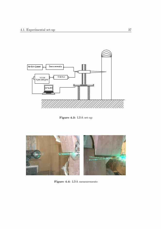
Figure 4.6: Vertical view of the guide vane profile
4.1.2 Flow measurement
Unfortunately, the chosen test loop did not contain any flow meters, thereforethe flow rate has been calculated by pitot measurement in the inlet pipe. Bymeasuring the velocity through the diameter of the pipe, the flow has been becalculated using equation (4.6):
Q =∫
UdA =∫ R
−R
u(r)2πrdr [m/s] (4.6)
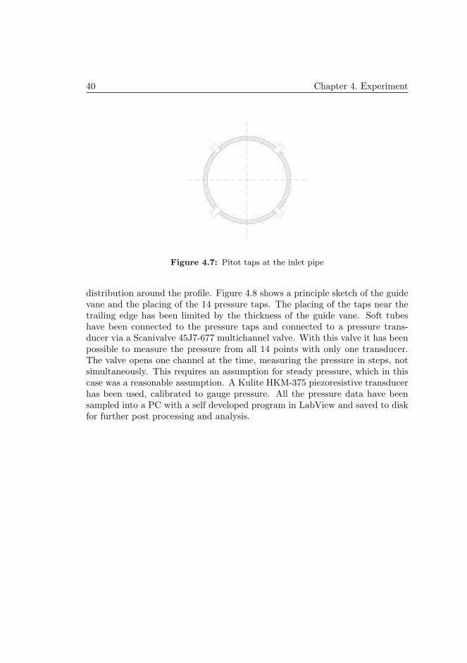
4 entrance holes have been made, 45on the centerline and 90on each other,see figure 4.7. The pitot probe covered 65 % of the pipe diameter and has beentraversed from all four holes, covering the whole diameter by good margin.
4.1.3 Guide vane pressure-profile
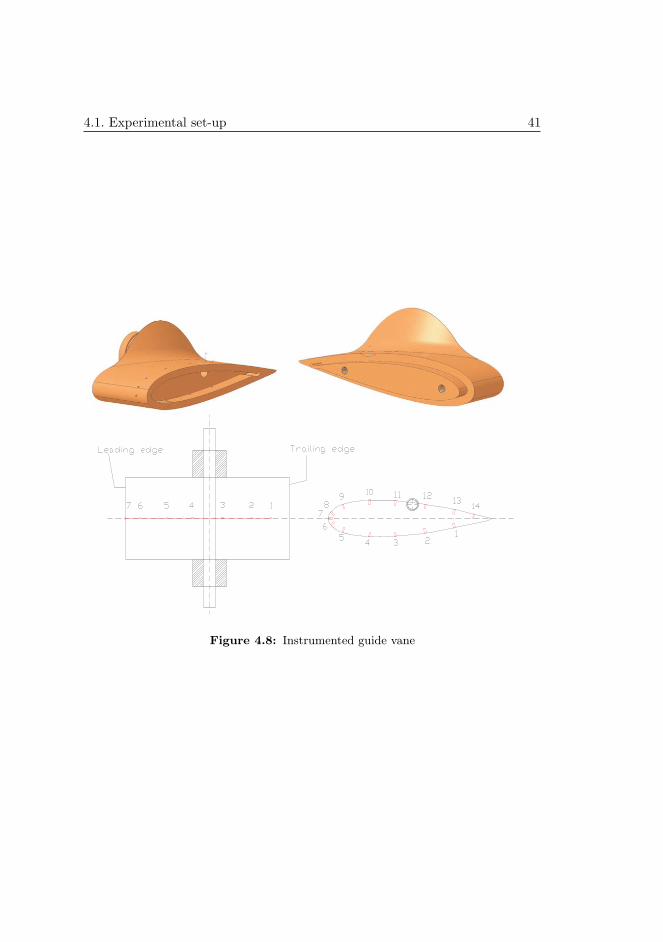
The middle guide vane for both profiles have been made hollow and instrumentedwith pressure taps around the whole profile in order to measure the pressure
40 Chapter 4. Experiment
Figure 4.7: Pitot taps at the inlet pipe
distribution around the profile. Figure 4.8 shows a principle sketch of the guidevane and the placing of the 14 pressure taps. The placing of the taps near thetrailing edge has been limited by the thickness of the guide vane. Soft tubeshave been connected to the pressure taps and connected to a pressure trans-ducer via a Scanivalve 45J7-677 multichannel valve. With this valve it has beenpossible to measure the pressure from all 14 points with only one transducer.The valve opens one channel at the time, measuring the pressure in steps, notsimultaneously. This requires an assumption for steady pressure, which in thiscase was a reasonable assumption. A Kulite HKM-375 piezoresistive transducerhas been used, calibrated to gauge pressure. All the pressure data have beensampled into a PC with a self developed program in LabView and saved to diskfor further post processing and analysis.
4.1. Experimental set-up 41
Figure 4.8: Instrumented guide vane
42 Chapter 4. Experiment
4.2 Experimental results
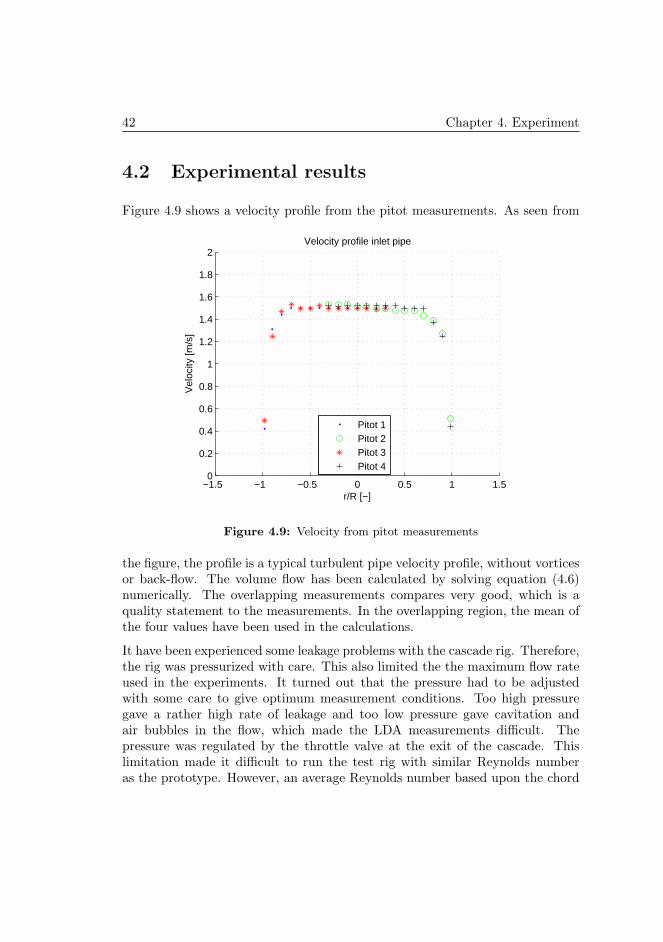
Figure 4.9 shows a velocity profile from the pitot measurements. As seen from
−1.5 −1 −0.5 0 0.5 1 1.50
0.2
0.4
0.6
0.8
1
1.2
1.4
1.6
1.8
2
r/R [−]
Vel
ocity
[m/s
]
Velocity profile inlet pipe
Pitot 1Pitot 2Pitot 3Pitot 4
Figure 4.9: Velocity from pitot measurements
the figure, the profile is a typical turbulent pipe velocity profile, without vorticesor back-flow. The volume flow has been calculated by solving equation (4.6)numerically. The overlapping measurements compares very good, which is aquality statement to the measurements. In the overlapping region, the mean ofthe four values have been used in the calculations.
It have been experienced some leakage problems with the cascade rig. Therefore,the rig was pressurized with care. This also limited the the maximum flow rateused in the experiments. It turned out that the pressure had to be adjustedwith some care to give optimum measurement conditions. Too high pressuregave a rather high rate of leakage and too low pressure gave cavitation andair bubbles in the flow, which made the LDA measurements difficult. Thepressure was regulated by the throttle valve at the exit of the cascade. Thislimitation made it difficult to run the test rig with similar Reynolds numberas the prototype. However, an average Reynolds number based upon the chord
4.2. Experimental results 43
length of the guide vane is of order of magnitude 2.5 · 106 while for the prototype,the average Reynolds number is of order of magnitude 4.5 · 106. This is assumedto be close enough for the purpose of the work within this thesis since there areno direct comparison between measurements on the prototype and on the model.The comparisons in this thesis are between the model test and CFD-calculationswhich have the same Reynolds number.
The maximum changes in the water temperature for all the experiments havebeen 5C, (19-24C). According to table B.3 in the IEC standard [29] this givesa variation in kinematic viscosity on 1.16 · 10−7m2/s, which has assumed not toinfluence on the results.
Since the main focus has been the influence of the guide vane profile on the flowfield, the major part of the measurements have been carried out at mid-span ofthe guide vane. According to Chen [14], the flow at the mid-span is the mostundisturbed flow since the influence of leakage flow and boundary layer of thefacing plates are negligible at this position.
As mentioned, it has been measured with two different sets of guide vanes. Thefirst set has been measured with three different flow rates and two different guidevane angles. During assembling of the new set of guide vanes, the fastening bolton one of the vanes broke. This required the vane to be welded to the rig in orderto be kept in place. Because of this it has not been possible to change the guidevane angle of the new set of vanes. Therefore, only changes in flow rate havebeen carried out with this set. It has been measured in different downstreampositions. Due to the angle of the laser beams, the point closest to the trailingedge possible to measure at mid-span is located about 11 mm from the trailingedge.
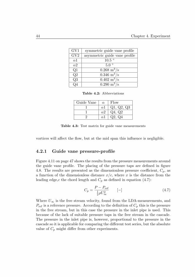
In the following sections, some abbreviations have been used for simplificationsin captions and labels. An overview of these abbreviations are given in table4.2.
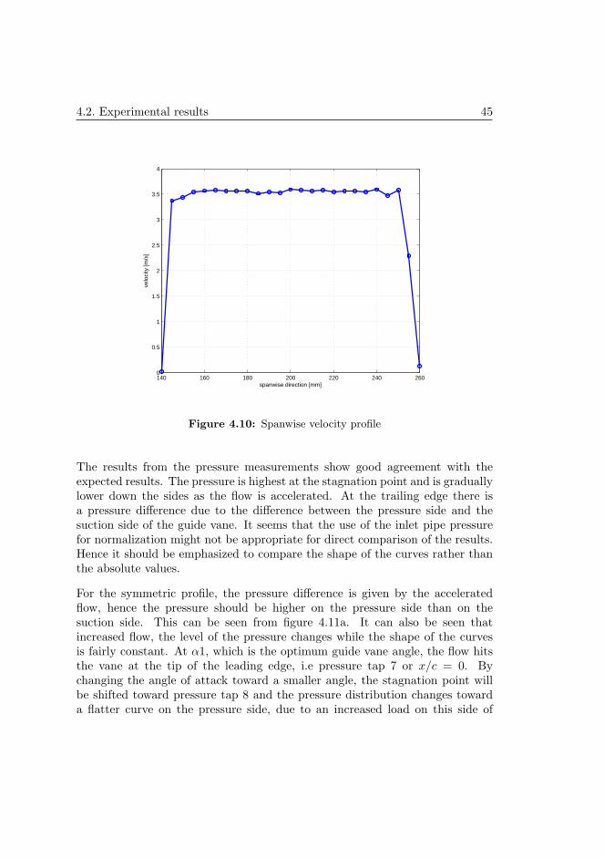
The test matrix for the measurements is shown in table 4.3. The pressurearound the guide vane profile has been measured for each of the cases in thetest matrix. First the velocity was measured in the free stream in span wisedirection to confirm that the flow field was uniform, without vortices or back-flow. As shown in figure 4.10 on page 45, the flow is quite uniform in thisdirection. These measurements have rather coarse steps and is conducted to seeif any large flow structures disturbs the mean flow at mid span. As measured byChen [14], influence from the boundary layer of the facing plates and horseshoe
44 Chapter 4. Experiment
GV1 symmetric guide vane profileGV2 asymmetric guide vane profileα1 10.5
α2 5.0
Q1 0.268 m3/sQ2 0.346 m3/sQ3 0.402 m3/sQ4 0.290 m3/s
Table 4.2: Abbreviations
Guide Vane α Flow1 α1 Q1, Q2, Q31 α2 Q4, Q22 α1 Q2, Q4
Table 4.3: Test matrix for guide vane measurements
vortices will affect the flow, but at the mid span this influence is negligible.
4.2.1 Guide vane pressure-profile
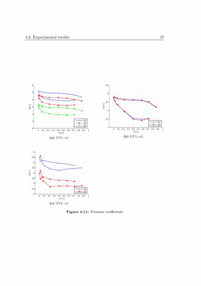
Figure 4.11 on page 47 shows the results from the pressure measurements aroundthe guide vane profile. The placing of the pressure taps are defined in figure4.8. The results are presented as the dimensionless pressure coefficient, Cp, asa function of the dimensionless distance x/c, where x is the distance from theleading edge,c the chord length and Cp as defined in equation (4.7):
Cp =P − Pref
12ρU2
∞[−] (4.7)
Where U∞ is the free stream velocity, found from the LDA-measurements, andPref is a reference pressure. According to the definition of Cp this is the pressurein the free stream, but in this case the pressure in the inlet pipe is used. Thisbecause of the lack of suitable pressure taps in the free stream in the cascade.The pressure in the inlet pipe is, however, proportional to the pressure in thecascade so it is applicable for comparing the different test series, but the absolutevalue of Cp might differ from other experiments.
4.2. Experimental results 45
140 160 180 200 220 240 2600
0.5
1
1.5
2
2.5
3
3.5
4
spanwise direction [mm]
velo
city
[m/s
]
Figure 4.10: Spanwise velocity profile
The results from the pressure measurements show good agreement with theexpected results. The pressure is highest at the stagnation point and is graduallylower down the sides as the flow is accelerated. At the trailing edge there isa pressure difference due to the difference between the pressure side and thesuction side of the guide vane. It seems that the use of the inlet pipe pressurefor normalization might not be appropriate for direct comparison of the results.Hence it should be emphasized to compare the shape of the curves rather thanthe absolute values.
For the symmetric profile, the pressure difference is given by the acceleratedflow, hence the pressure should be higher on the pressure side than on thesuction side. This can be seen from figure 4.11a. It can also be seen thatincreased flow, the level of the pressure changes while the shape of the curvesis fairly constant. At α1, which is the optimum guide vane angle, the flow hitsthe vane at the tip of the leading edge, i.e pressure tap 7 or x/c = 0. Bychanging the angle of attack toward a smaller angle, the stagnation point willbe shifted toward pressure tap 8 and the pressure distribution changes towarda flatter curve on the pressure side, due to an increased load on this side of
46 Chapter 4. Experiment
the vane. Since the distance between the vanes is decreased, the same flow ratemust have a higher velocity and hence a higher acceleration from the stagnationpoint and the pressure difference between suction side and pressure side willincrease. With the asymmetric profile, the pressure side and suction side shouldbe opposite of the symmetric profile, according to the hypothesis presented inchapter 1. Figure 4.11c shows that this actually is the case.
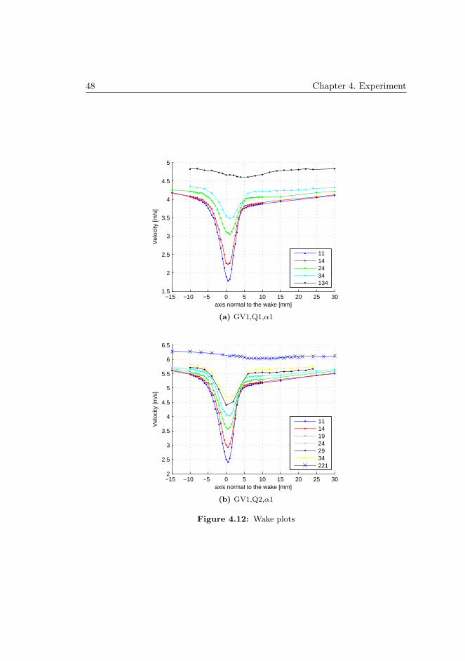
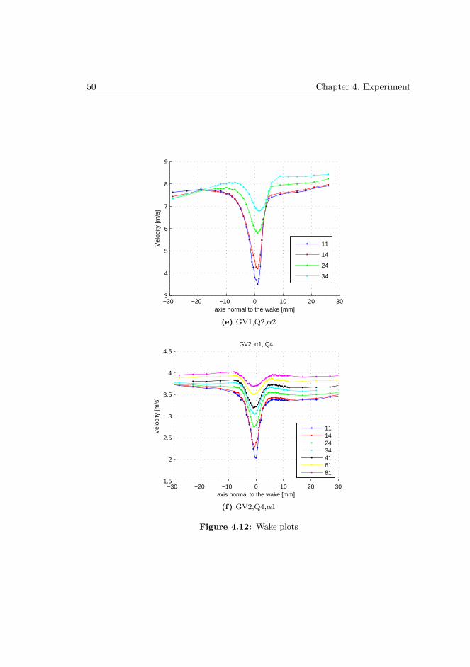
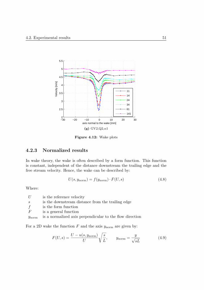
4.2.2 Wake plots
Figure 4.12 shows the results from the LDA measurements. The legends indicatethe length downstream from the trailing edge of the guide vane in mm. Notethat the scale is different for each plot in order to optimize the visualization ofeach wake. The horizontal axis is zero at the trailing edge of the guide vaneand the positive side is the ’free stream side’ while the negative side ends in thecorresponding guide vane.
The figures show that the LDA-results seams reasonable at first glance. Thevelocity defect is decreasing and the width of the wake is increasing as thedistance from the guide vane is increasing. By increasing the flow, and hencethe free stream velocity, the velocity defect is increasing. This because of thedead water region right downstream the trailing edge. The velocity here is closeto zero and with an increase of the free stream velocity, the velocity defectshould also be increasing.
The results from the symmetric guide vane show that the wake is shifted slightlytoward the global suction side, while with the asymmetric profile the wake ismore right downstream the guide vane and it is even a tendency that it is shiftedtoward the global pressure side. This indicates that the change of guide vaneprofile actually changes the pressure distribution at the outlet of the guide vanes.
According to Bernoulli’s equation the velocity should be higher on the suctionside and lower on the pressure side, causing a skewness in the velocity plots.This is found in the measurements from the smaller guide vane opening, 5.0 ,but for the the guide vane opening at 10.5 the tendency is rather the opposite.One explanation might be that at this opening, the pressure difference is to smallto have any significant influence on the flow field. Even though the skewnessis small, it changes with the change of pressure side according to the pressuremeasurements showed in figure 4.11 since the results from the asymmetric guidevane show a wake skewed in the opposite direction.
4.2. Experimental results 47
0 0.1 0.2 0.3 0.4 0.5 0.6 0.7 0.8 0.9 10
1
2
3
4
5
6
x/c [−]
Cp
[−]
Q1Q2Q3
(a) GV1, α1
0 0.1 0.2 0.3 0.4 0.5 0.6 0.7 0.8 0.9 11
1.5
2
2.5
3
3.5
x/c [−]
Cp
[−]
Q4Q2
(b) GV1, α2
0 0.1 0.2 0.3 0.4 0.5 0.6 0.7 0.8 0.9 12
2.5
3
3.5
4
4.5
5
5.5
6
x/c [−]
Cp
[−]
Q4Q2
(c) GV2, α1
Figure 4.11: Pressure coefficients
48 Chapter 4. Experiment
−15 −10 −5 0 5 10 15 20 25 301.5
2
2.5
3
3.5
4
4.5
5
axis normal to the wake [mm]
Vel
ocity
[m/s
]
11142434134
(a) GV1,Q1,α1
−15 −10 −5 0 5 10 15 20 25 302
2.5
3
3.5
4
4.5
5
5.5
6
6.5
axis normal to the wake [mm]
Vel
ocity
[m/s
]
111419242934221
(b) GV1,Q2,α1
Figure 4.12: Wake plots

4.2. Experimental results 49
−15 −10 −5 0 5 10 15 20 25 302
3
4
5
6
7
8
9
axis normal to the wake [mm]
Vel
ocity
[m/s
]
11
14
24
34
134
(c) GV1,Q3,α1
−30 −20 −10 0 10 20 302
3
4
5
6
7
8
axis normal to the wake [mm]
Vel
ocity
[m/s
]
11
14
24
34
(d) GV1,Q4,α2
Figure 4.12: Wake plots
50 Chapter 4. Experiment
−30 −20 −10 0 10 20 303
4
5
6
7
8
9
axis normal to the wake [mm]
Vel
ocity
[m/s
]
11
14
24
34
(e) GV1,Q2,α2
−30 −20 −10 0 10 20 301.5
2
2.5
3
3.5
4
4.5
axis normal to the wake [mm]
Vel
ocity
[m/s
]
GV2, α1, Q4
11142434416181
(f) GV2,Q4,α1
Figure 4.12: Wake plots
4.2. Experimental results 51
−30 −20 −10 0 10 20 302
2.5
3
3.5
4
4.5
5
5.5
axis normal to the wake [mm]
Vel
ocity
[m/s
]
11
14
24
34
61
141
(g) GV2,Q2,α1
Figure 4.12: Wake plots
4.2.3 Normalized results
In wake theory, the wake is often described by a form function. This functionis constant, independent of the distance downstream the trailing edge and thefree stream velocity. Hence, the wake can be described by:
U(s, ynorm) = f(ynorm) ·F (U, s) (4.8)
Where:
U is the reference velocitys is the downstream distance from the trailing edgef is the form functionF is a general functionynorm is a normalized axis perpendicular to the flow direction
For a 2D wake the function F and the axis ynorm are given by:
F (U, s) =U − u(s, ynorm)
U
√s
L, ynorm =
y√sL
(4.9)
52 Chapter 4. Experiment
L is a reference distance, typically the chord length.
If F and ynorm are correct, the form function, f should be independent of thedownstream length, s. In the guide vane cascade, the free stream velocity isan accelerated flow, hence the reference velocity, U , was set to the free streamvelocity for each measurement.
It is assumed that the following function is a suitable form function for the wake:
unorm = a + b · ec(x−d)2 (4.10)
The coefficients are defined in figure 4.13 on the facing page. It should be notedthat the coefficient c describes the width of the wake with a relative value. Thecloser to zero, the wider wake and the more negative, the narrower wake. Theother coefficients describes the wake with values directly from the plot.
The velocity is normalized by the free stream velocity at each s, since it is anaccelerated flow:
unorm =u− U(s)
U(s)(4.11)
Then the normalized velocity defect, b, is plotted as a function of downstreamlength, see figure 4.14 on the next page. As seen from the figure, the normalizedvalues show good agreement within the different test series.
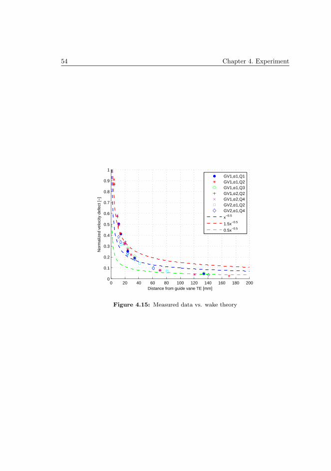
Figure 4.15 on page 54 shows the three functions x−0.5, 1.5x−0.5 and 0.5x−0.5
for comparison with the wake-theory.
It can be seen from the figure that the self similar zone starts at about 40 mmdownstream the trailing edge or x/c ≈ 0.12. Since this method ’forces’ the waketo fit a symmetric curve, this analysis will be a pure viscous analysis, not takinginto account the effect of the velocity difference of the pressure side and suctionside of the guide vane. However it will describe how the flow fits into traditionalviscous wake theory, and if this theory is useful for this type of flow. Also, asthe velocity plots have shown, this effect is rather small in this case.
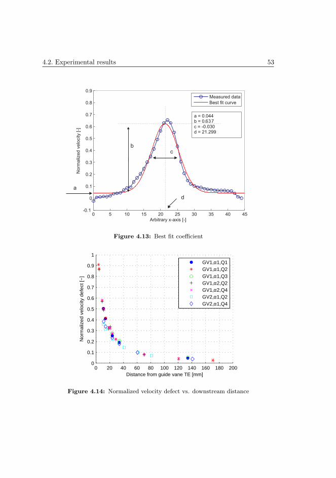
4.2. Experimental results 53
a
c
d
b
Figure 4.13: Best fit coefficient
0 20 40 60 80 100 120 140 160 180 2000
0.1
0.2
0.3
0.4
0.5
0.6
0.7
0.8
0.9
1
Distance from guide vane TE [mm]
Nor
mal
ized
vel
ocity
def
ect [
−]
GV1,α1,Q1GV1,α1,Q2GV1,α1,Q3GV1,α2,Q2GV1,α2,Q4GV2,α1,Q2GV2,α1,Q4
Figure 4.14: Normalized velocity defect vs. downstream distance
54 Chapter 4. Experiment
0 20 40 60 80 100 120 140 160 180 2000
0.1
0.2
0.3
0.4
0.5
0.6
0.7
0.8
0.9
1
Distance from guide vane TE [mm]
Nor
mal
ized
vel
ocity
def
ect [
−]
GV1,α1,Q1GV1,α1,Q2GV1,α1,Q3GV1,α2,Q2GV1,α2,Q4GV2,α1,Q2GV2,α1,Q4
x−0.5
1.5x−0.5
0.5x−0.5
Figure 4.15: Measured data vs. wake theory
4.2. Experimental results 55
4.2.4 Wake in span-wise direction
Figure 4.16 on page 57 shows velocity plots of the velocity in constant down-stream distance and varying span-wise direction. The span-wise direction isfrom the middle and out to the facing plate. As seen from the figures, the ve-locity defect is increasing and lightly more shifted toward the global pressureside. This increase in wake might be caused by the ’ears’ of the guide vanes.These ears will increase the cross-section area, causing a larger wake locally.Comparing the wake at the same distance from the mid span but in oppositedirection, as shown in figure 4.17 on page 57, shows quite good, but not exactlyagreement. A common assumption is to assume the flow symmetric around themid span of the guide vanes, but this results show that this may not always betrue.
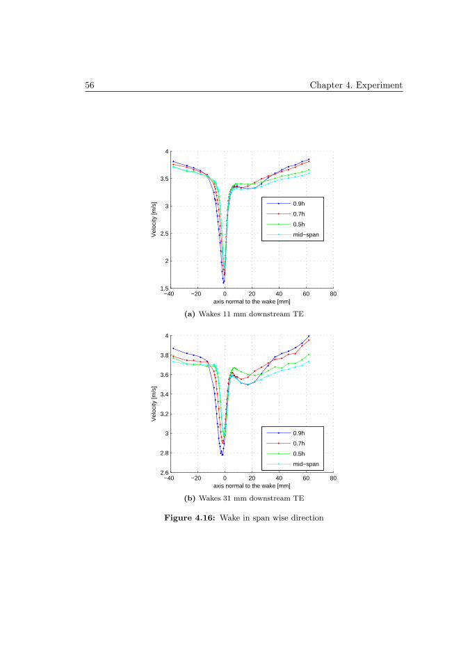
56 Chapter 4. Experiment
−40 −20 0 20 40 60 801.5
2
2.5
3
3.5
4
axis normal to the wake [mm]
Vel
ocity
[m/s
]
0.9h
0.7h
0.5h
mid−span
(a) Wakes 11 mm downstream TE
−40 −20 0 20 40 60 802.6
2.8
3
3.2
3.4
3.6
3.8
4
axis normal to the wake [mm]
Vel
ocity
[m/s
]
0.9h
0.7h
0.5h
mid−span
(b) Wakes 31 mm downstream TE
Figure 4.16: Wake in span wise direction
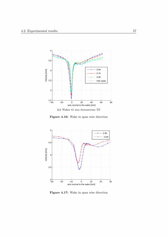
4.2. Experimental results 57
−40 −20 0 20 40 60 801.5
2
2.5
3
3.5
4
axis normal to the wake [mm]
Vel
ocity
[m/s
]
0.9h
0.7h
0.5h
mid−span
(c) Wakes 41 mm downstream TE
Figure 4.16: Wake in span wise direction
−30 −20 −10 0 10 20 303
3.5
4
4.5
5
axis normal to the wake [mm]
Vel
ocity
[m/s
]
0.9h
−0.9h
Figure 4.17: Wake in span wise direction
58 Chapter 4. Experiment
4.3 Summary
During start up and shut down of the rig, the pressure was lowed so air bubbleswere visible in the water. At this operation points, a vortex was observed at theinner curve, approximately at the height of guide vane 3 and 4. Unfortunately,this was outside the range of the traverse table so it could not be confirmedwhether this vortex was present during the measurements or not. If the vortexwas present, the velocity in the measurement section would be higher thanexpected from the calculated flow rate.
It was assumed that the horseshoe vortices close to the facing plates wouldcontribute to increase the mixing in the flow and hence cause a smaller wakecloser to the facing plates, but the results actually showed the opposite effect.This is probably caused by the increased area due to the ears on the guide vanesand that the horseshoe vortices not affect the flow so far from the facing plates.
In addition to the velocity defect itself, the wake will also cause a change in thedirection of the relative velocity at the inlet of the runner blade. This velocitychange will cause the inlet flow angle, β in figure 2.6 on page 10, to vary whichwill cause a varying load on the runner blade. This variation is analogous to achange in the angle of attack on a wing profile. The change in angle of attackwill change the lift force on the wing, and similarly, the change in the flowangle on the runner blade will cause a varying load on the runner blade. Sincethis change is caused by the wake of the guide vanes, the runner blade will feelthis change every time a it passes a guide vane, resulting in a varying load onthe blade. This effect is dependent on the wake and the distance between theguide vane and runner. This means that the wake will be largest at full loadwhen the guide vanes are fully open and, hence, the distance between the guidevane and runner blade are at a minimum. Kjeldesen [37] derived the changeof pressure caused by change in the relative velocity for a typically high headFrancis turbine and found that the pressure might vary between 1% up to 11%of the turbine’s net head with the highest value for full load.
4.4 Estimated experimental uncertainty
All measurements have errors. These errors are the difference between the mea-sured value and the true value. The total error, F , have two components: biaserror, b, and random error, s. When these components are combined in a single
4.4. Estimated experimental uncertainty 59
uncertainty number, F , the true value, V , lies within the interval:
V = X ± F (4.12)
Where X, is the sample average of the measured quantity. The individualuncertainty, Fi is defined in the standard ISO/TR 5168, [30] as:
Fi =√
b2 + (t95 · s)2 (4.13)
where b is the systematic uncertainty of a symmetric uncertainty interval, s theexperimental standard deviation of the mean and t95 the 95th percentile pointof the two tailed Student-t distribution. When the individual uncertainty isfound, the overall uncertainty is found from:
F =
√√√√ n∑i=1
F 2i (4.14)
In cases where the wanted parameter is calculated as a function of a measuredquantity, errors in the measurements are propagated to the quantity through thefunction. This effect may be approximated with the Taylor series method, intro-ducing the sensitivity coefficient, θ. Given the parameter R = f(Y1, Y 2, ...Yn),θ can be calculated by:
θi =∂R
∂Yi(4.15)
The dimensionless sensitivity coefficient can now be calculated as:
θ∗i = θiYi
R(4.16)
For the pitot measurements the velocity is a function of the pressure difference inthe pitot tube, given by a measured height of water column in the manometer,h.Thus the velocity can be expressed by:
v =√
2 · g ·h [m/s] (4.17)
The sensitivity coefficient can now be calculated as:
θ =∂v
∂h=
∂(√
2 · g ·h)∂h
=12· vh
(4.18)
θ∗ =12
v
h· hv
=12
(4.19)
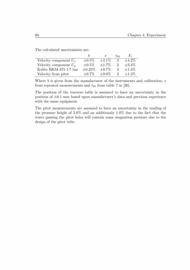
60 Chapter 4. Experiment
The calculated uncertainties are:
b s t95 Fi
Velocity component Ux ±0.5% ±2.1% 2 ±4.2%Velocity component Uy ±0.5% ±1.7% 2 ±3.4%Kulite HKM-375 1.7 bar ±0.25% ±0.7% 2 ±1.4%Velocity from pitot ±0.7% ±0.8% 2 ±1.3%
Where b is given from the manufacturer of the instruments and calibration, sfrom repeated measurements and t95 from table 7 in [30].
The position of the traverse table is assumed to have an uncertainty in theposition of ±0.1 mm based upon manufacturer’s data and previous experiencewith the same equipment.
The pitot measurements are assumed to have an uncertainty in the reading ofthe pressure height of 2.0% and an additionaly 1.0% due to the fact that thewater passing the pitot holes will contain some stagnation pressure due to thedesign of the pitot tube.

Chapter 5
Comparison of numericaland experimental results
5.1 Comparison
The numerical results have been compared with the measurements by plots ofvelocity magnitude in the wake downstream the guide vanes. Figure 5.1 onthe following page shows a comparison of velocity plots from LDA and CFDat different downstream positions. The figure shows that the wakes from theCFD-calculations have fairly the same shape as the measured one, and that theposition of the wake has been very good captured. However, the CFD resultsshow a higher free stream velocity and a narrower and less deep velocity defect.An average of all the calculations show an over-prediction of the free streamvelocity of ca 15 %, an under-prediction of the depth and width of the wake ofca 25 % and 30 % respectively. The CFD-plots also show a tendency to be moreskewed than the measured one.
It has not been surprising that the wakes have been under-predicted in thiscalculations since quite a few simplifications have been made. The CFD-modelused is a 2-dimensional model, while the results from the LDA-measurementshave shown that the velocity defect also will vary in the span wise direction.This means that there must be momentum transfer in this direction which again
61
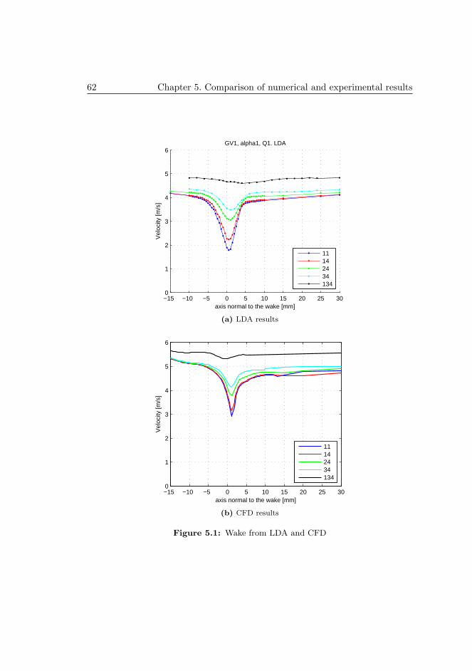
62 Chapter 5. Comparison of numerical and experimental results
−15 −10 −5 0 5 10 15 20 25 300
1
2
3
4
5
6
axis normal to the wake [mm]
Vel
ocity
[m/s
]
GV1, alpha1, Q1. LDA
11142434134
(a) LDA results
−15 −10 −5 0 5 10 15 20 25 300
1
2
3
4
5
6
axis normal to the wake [mm]
Vel
ocity
[m/s
]
11142434134
(b) CFD results
Figure 5.1: Wake from LDA and CFD
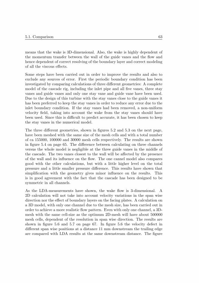
5.1. Comparison 63
means that the wake is 3D-dimensional. Also, the wake is highly dependent ofthe momentum transfer between the wall of the guide vanes and the flow andhence dependent of correct resolving of the boundary layer and correct modelingof all the viscous effects.
Some steps have been carried out in order to improve the results and also toexclude any sources of error. First the periodic boundary condition has beeninvestigated by comparing calculations of three different geometries: A completemodel of the cascade rig, including the inlet pipe and all five vanes, three stayvanes and guide vanes and only one stay vane and guide vane have been used.Due to the design of this turbine with the stay vanes close to the guide vanes ithas been preferred to keep the stay vanes in order to reduce any error due to theinlet boundary condition. If the stay vanes had been removed, a non-uniformvelocity field, taking into account the wake from the stay vanes should havebeen used. Since this is difficult to predict accurate, it has been chosen to keepthe stay vanes in the numerical model.
The three different geometries, shown in figures 5.2 and 5.3 on the next page,have been meshed with the same size of the mesh cells and with a total numberof ca 155000, 100000 and 30000 mesh cells respectively. The results are shownin figure 5.4 on page 65. The difference between calculating on three channelsversus the whole model is negligible at the three guide vanes in the middle ofthe cascade. The two vanes closest to the wall will be affected by the presenceof the wall and its influence on the flow. The one cannel model also comparesgood with the other calculations, but with a little higher level on the totalpressure and a little smaller pressure difference. This results have shown thatsimplification with the geometry gives minor influence on the results. Thisis in good agreement with the fact that the cascade has been designed to besymmetric in all channels.
As the LDA-measurements have shown, the wake flow is 3-dimensional. A2D calculation will not take into account velocity variations in the span wisedirection nor the effect of boundary layers on the facing plates. A calculation ona 3D model, with only one channel due to the mesh size, has been carried out inorder to achieve a more realistic flow pattern. Even with only one channel, a 3D-mesh with the same cell-size as the optimum 2D-mesh will have about 500000mesh cells, dependent of the resolution in span wise direction. The results areshown in figure 5.6 and 5.7 on page 67. In figure 5.6 the velocity defect indifferent span wise positions at a distance 11 mm downstream the trailing edgeare compared with LDA results at the same downstream distance. The figure
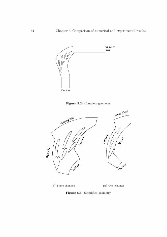
64 Chapter 5. Comparison of numerical and experimental results
Figure 5.2: Complete geometry
!
"$#&% ' ()+*
,.-0/214325 67 598 / - 6
:4; <=> ? =@
ACB DEGF HEJI
K$L&M N OP+Q
(a) Three channels (b) One channel
Figure 5.3: Simplified geometry
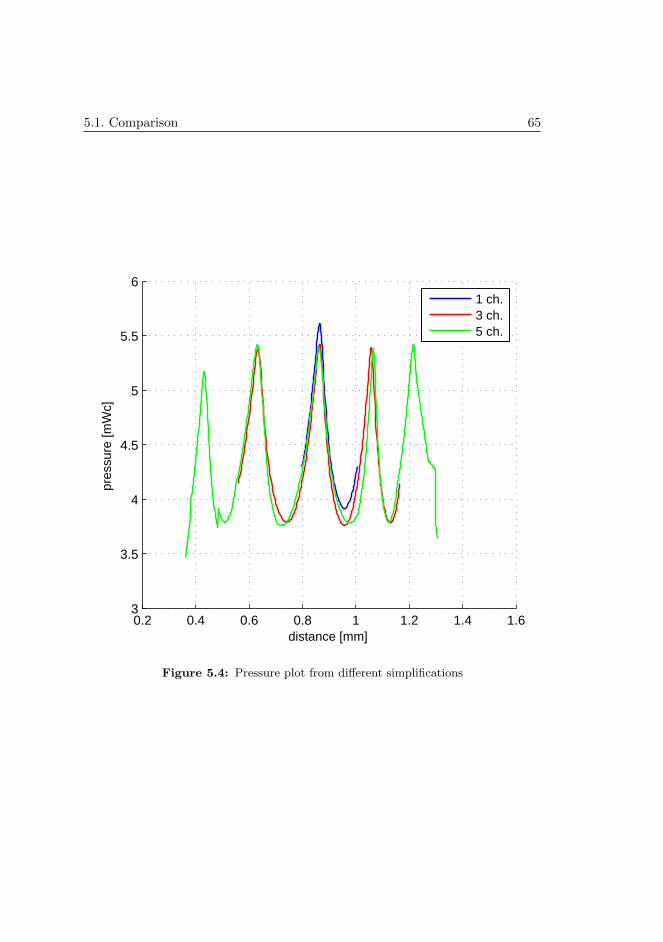
5.1. Comparison 65
0.2 0.4 0.6 0.8 1 1.2 1.4 1.63
3.5
4
4.5
5
5.5
6
distance [mm]
pres
sure
[mW
c]
1 ch.3 ch.5 ch.
Figure 5.4: Pressure plot from different simplifications

66 Chapter 5. Comparison of numerical and experimental results
Figure 5.5: 3D Mesh around the guide vane
shows that the CFD still under-predicts the depth of the wake, but the widthand free stream velocity have been better captured. An average of all the 3D-calculations gives an over-prediction of the free stream velocity of ca 5 % andan under-prediction of the depth and width of ca 15 % and 5 % respectively.Figure 5.7 shows that the CFD-calculations are much more symmetric aroundthe mid span than the LDA-measurements. This indicates that there have beensome factors in the cascade rig causing the flow to be non-uniform that not havebeen captured in the CFD calculations.
A difference between the experimental and numerical results has not been un-expected, since the experiment contained some factors that is hard to captureby CFD. It has been experienced quite a lot of small leakages on the model rig,which probably caused additional secondary flow and contributed to make theflow field non-uniform. Also the horse-shoe vortices at the facing plates willaffect the flow, but none of these effects will be captured in a CFD-model. Ithas also been observed a vortex at the inner curve of the cascade model, ap-proximately at the height of guide vane 4. This vortex has been visible due tothe low pressure with resolved air bubbles during start up and shut down of therig. The location of the vortex has been outside the traversing range of the LDAso it could not be confirmed whether it was present during the measurementsor not. Assuming the presence of a vortex, the main flow in the rest of the
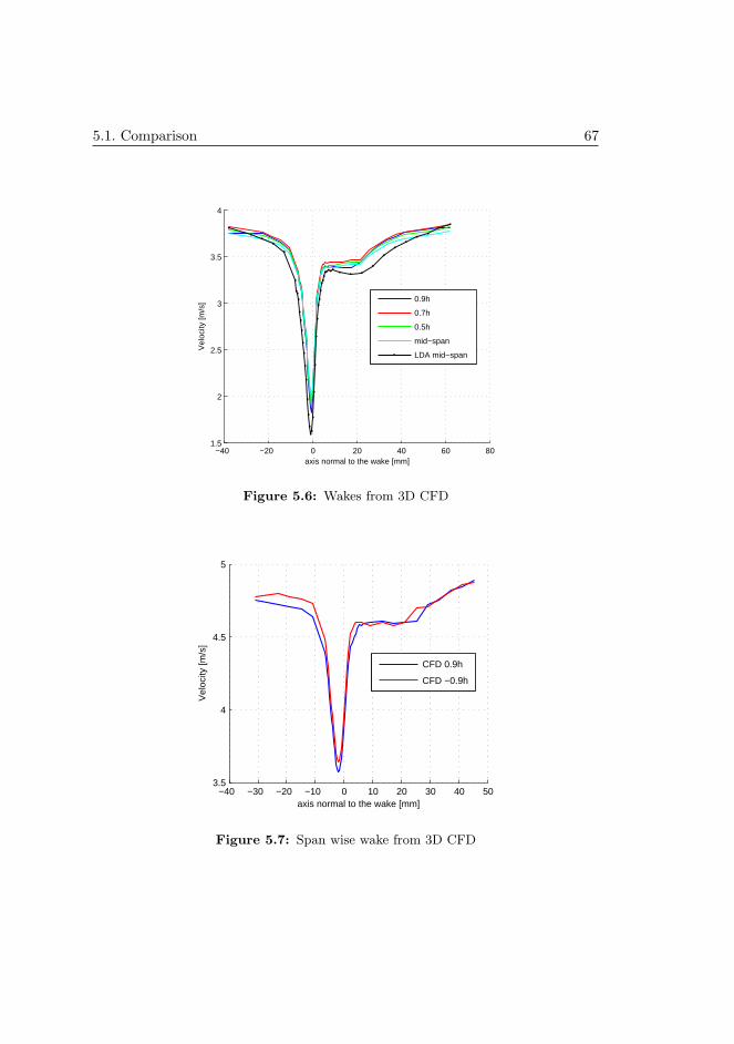
5.1. Comparison 67
−40 −20 0 20 40 60 801.5
2
2.5
3
3.5
4
axis normal to the wake [mm]
Vel
ocity
[m/s
]
0.9h
0.7h
0.5h
mid−span
LDA mid−span
Figure 5.6: Wakes from 3D CFD
−40 −30 −20 −10 0 10 20 30 40 503.5
4
4.5
5
axis normal to the wake [mm]
Vel
ocity
[m/s
]
CFD 0.9h
CFD −0.9h
Figure 5.7: Span wise wake from 3D CFD
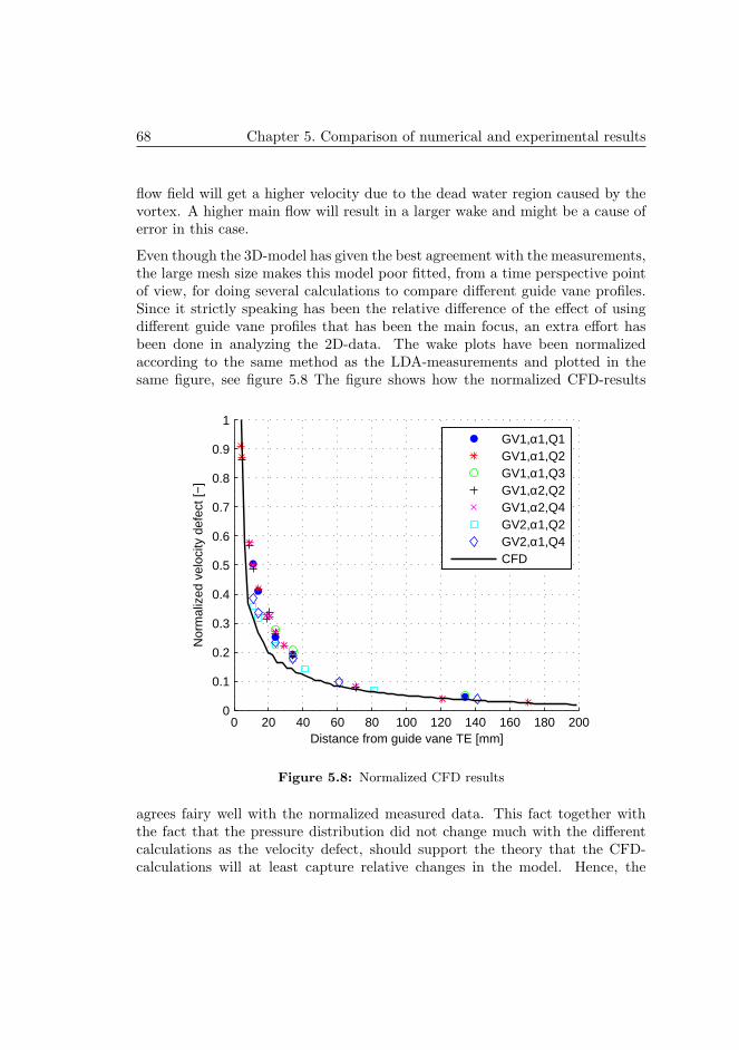
68 Chapter 5. Comparison of numerical and experimental results
flow field will get a higher velocity due to the dead water region caused by thevortex. A higher main flow will result in a larger wake and might be a cause oferror in this case.
Even though the 3D-model has given the best agreement with the measurements,the large mesh size makes this model poor fitted, from a time perspective pointof view, for doing several calculations to compare different guide vane profiles.Since it strictly speaking has been the relative difference of the effect of usingdifferent guide vane profiles that has been the main focus, an extra effort hasbeen done in analyzing the 2D-data. The wake plots have been normalizedaccording to the same method as the LDA-measurements and plotted in thesame figure, see figure 5.8 The figure shows how the normalized CFD-results
0 20 40 60 80 100 120 140 160 180 2000
0.1
0.2
0.3
0.4
0.5
0.6
0.7
0.8
0.9
1
Distance from guide vane TE [mm]
Nor
mal
ized
vel
ocity
def
ect [
−]
GV1,α1,Q1GV1,α1,Q2GV1,α1,Q3GV1,α2,Q2GV1,α2,Q4GV2,α1,Q2GV2,α1,Q4CFD
Figure 5.8: Normalized CFD results
agrees fairy well with the normalized measured data. This fact together withthe fact that the pressure distribution did not change much with the differentcalculations as the velocity defect, should support the theory that the CFD-calculations will at least capture relative changes in the model. Hence, the
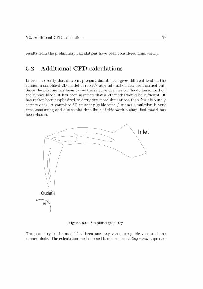
5.2. Additional CFD-calculations 69
results from the preliminary calculations have been considered trustworthy.
5.2 Additional CFD-calculations
In order to verify that different pressure distribution gives different load on therunner, a simplified 2D model of rotor/stator interaction has been carried out.Since the purpose has been to see the relative changes on the dynamic load onthe runner blade, it has been assumed that a 2D model would be sufficient. Ithas rather been emphasized to carry out more simulations than few absolutelycorrect ones. A complete 3D unsteady guide vane / runner simulation is verytime consuming and due to the time limit of this work a simplified model hasbeen chosen.
Inlet
Outlet
Figure 5.9: Simplified geometry
The geometry in the model has been one stay vane, one guide vane and onerunner blade. The calculation method used has been the sliding mesh approach
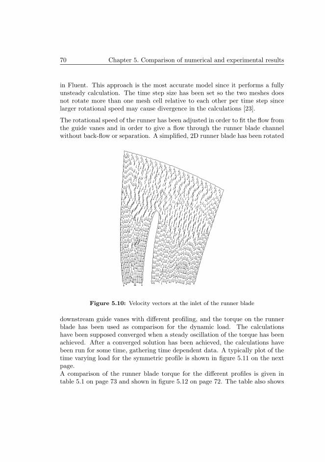
70 Chapter 5. Comparison of numerical and experimental results
in Fluent. This approach is the most accurate model since it performs a fullyunsteady calculation. The time step size has been set so the two meshes doesnot rotate more than one mesh cell relative to each other per time step sincelarger rotational speed may cause divergence in the calculations [23].
The rotational speed of the runner has been adjusted in order to fit the flow fromthe guide vanes and in order to give a flow through the runner blade channelwithout back-flow or separation. A simplified, 2D runner blade has been rotated
Figure 5.10: Velocity vectors at the inlet of the runner blade
downstream guide vanes with different profiling, and the torque on the runnerblade has been used as comparison for the dynamic load. The calculationshave been supposed converged when a steady oscillation of the torque has beenachieved. After a converged solution has been achieved, the calculations havebeen run for some time, gathering time dependent data. A typically plot of thetime varying load for the symmetric profile is shown in figure 5.11 on the nextpage.A comparison of the runner blade torque for the different profiles is given intable 5.1 on page 73 and shown in figure 5.12 on page 72. The table also shows
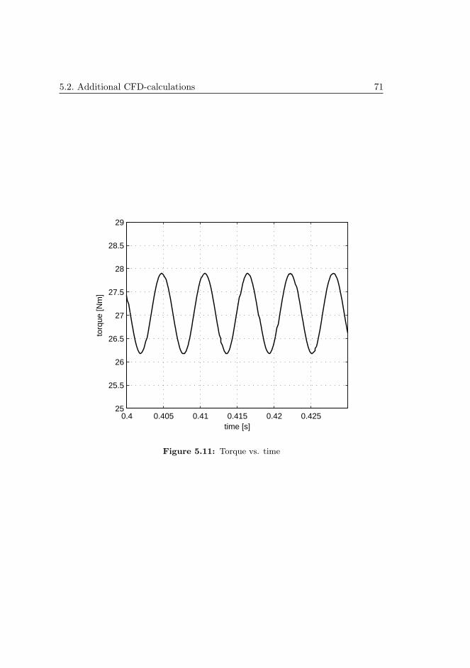
5.2. Additional CFD-calculations 71
0.4 0.405 0.41 0.415 0.42 0.42525
25.5
26
26.5
27
27.5
28
28.5
29
time [s]
torq
ue [N
m]
Figure 5.11: Torque vs. time
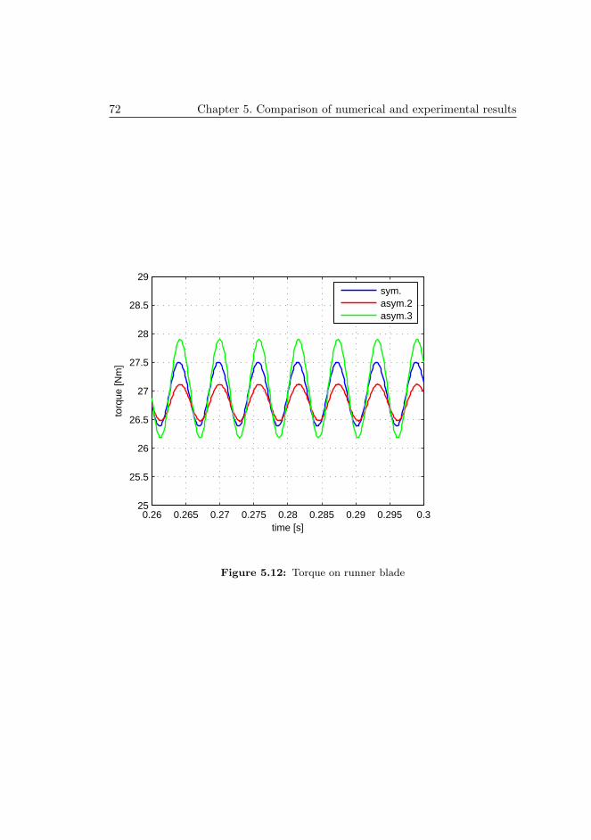
72 Chapter 5. Comparison of numerical and experimental results
0.26 0.265 0.27 0.275 0.28 0.285 0.29 0.295 0.325
25.5
26
26.5
27
27.5
28
28.5
29
time [s]
torq
ue [N
m]
sym.asym.2asym.3
Figure 5.12: Torque on runner blade
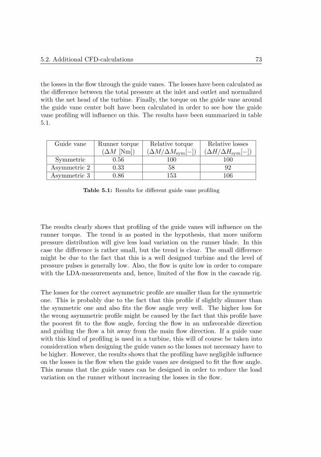
5.2. Additional CFD-calculations 73
the losses in the flow through the guide vanes. The losses have been calculated asthe difference between the total pressure at the inlet and outlet and normalizedwith the net head of the turbine. Finally, the torque on the guide vane aroundthe guide vane center bolt have been calculated in order to see how the guidevane profiling will influence on this. The results have been summarized in table5.1.
Guide vane Runner torque Relative torque Relative losses(∆M [Nm]) (∆M/∆Msym[−]) (∆H/∆Hsym[−])
Symmetric 0.56 100 100Asymmetric 2 0.33 58 92Asymmetric 3 0.86 153 106
Table 5.1: Results for different guide vane profiling
The results clearly shows that profiling of the guide vanes will influence on therunner torque. The trend is as posted in the hypothesis, that more uniformpressure distribution will give less load variation on the runner blade. In thiscase the difference is rather small, but the trend is clear. The small differencemight be due to the fact that this is a well designed turbine and the level ofpressure pulses is generally low. Also, the flow is quite low in order to comparewith the LDA-measurements and, hence, limited of the flow in the cascade rig.
The losses for the correct asymmetric profile are smaller than for the symmetricone. This is probably due to the fact that this profile if slightly slimmer thanthe symmetric one and also fits the flow angle very well. The higher loss forthe wrong asymmetric profile might be caused by the fact that this profile havethe poorest fit to the flow angle, forcing the flow in an unfavorable directionand guiding the flow a bit away from the main flow direction. If a guide vanewith this kind of profiling is used in a turbine, this will of course be taken intoconsideration when designing the guide vanes so the losses not necessary have tobe higher. However, the results shows that the profiling have negligible influenceon the losses in the flow when the guide vanes are designed to fit the flow angle.This means that the guide vanes can be designed in order to reduce the loadvariation on the runner without increasing the losses in the flow.

74 Chapter 5. Comparison of numerical and experimental results
5.3 Summary
After the numerical and experimental results have been compared, it can beconcluded that the CFD gives acceptable results. Even if the absolute cor-rect values have not been achieved, the normalized results have shown that thephysics of the flow has been well captured. Hence, it should be reasonable toassume that relative changes in the geometry would be captured in a good waywith CFD.
It is no doubt that correct profiling of the guide vanes can influence on thepressure distribution and that a more uniform pressure distribution reduces thedynamic load on the runner. This can be achieved without increasing the lossesin the flow.
There has not been carried out any calculations regarding the efficiency of theturbine, but it is assumed that as long as the flow from the guide vanes stillgives optimal inlet conditions on the runner, the efficiency should not have tobe sacrificed to achieve reduced load on the runner blades.
Chapter 6
Conclusions and furtherwork
6.1 Conclusions
An experimental and numerical study of the unsteady flow at the inlet of therunner of a Francis turbine has been carried out. The main goal has beento investigate how the profiling of the wicket gate can contribute to reducethe dynamic load on the runner blades by creating a more uniform pressuredistribution at the inlet of the runner.
LDA measurements in a cascade rig have shown that the viscous wake behindthe guide vanes can be described by classic wake theory, even though it is atendency that the wakes mixes out somewhat faster, due to the accelerated flowfield.
The CFD calculations have shown a tendency to under-estimate the wake andover-estimate the free stream velocity. This might be because of CFD’s lack ofresolving all the momentum transfers between the guide vanes and the water.In this case there have also been some uncertainties in the measurements dueto leakage flow over the guide vane and extra leakage in the cascade rig whichhave caused secondary flow which not has been captured by the CFD. The 2D-calculations have shown a deviation from the measurements with ca 25 %, while
75
76 Chapter 6. Conclusions and further work
the 3D-calculations have a deviation of ca 15 %, which has been assumed to beacceptable. This has shown that the wake flow is 3-dimensional with momentumtransfer in all directions. Still, 2D-calculations have given good agreement withthe relative, normalized results. This has indicated that even simplified 2D-calculations will be suitable to capture relative changes, even tough the absolutevalues might differ from the measurements.
Pressure measurements around the the mid-span of a guide vane have shownthat the pressure distribution has been according to the expected results. With asymmetric profile, the pressure is highest at the stagnation point and the guidevane will have a pressure distribution given by the flow field with a certainpressure side and suction side at the trailing edge. By changing the angle ofattack, the stagnation point will move according to the new flow angle. Byprofiling the guide vane asymmetric, the pressure side and suction side on theguide vane is either shifted or amplified. CFD-calculations have shown that withthe local pressure and suction side on the guide vane opposite to the one causedby the accelerated flow, the pressure will counteract and cause a more uniformoverall pressure distribution. Unsteady CFD-calculations of a simplified wicketgate / runner interaction have shown that a more uniform pressure distributionwill give less torque variation on the runner blade. Hence the profiling of theguide vanes might be designed in order to reduce the dynamic load on the runnerblades. This profiling have not increased the loss in the flow past the guide vaneswhich means that reducing the dynamic load on the runner should not reducethe efficiency of the turbine.
It should also be mentioned that even tough this profiling tends to reduce thedynamic load on the runner, turbines might very well operate smoothly evenwith the ’wrong’ profiling on the wicket gate. Together with the parametersdiscussed in this thesis, the distance between the wicket gate and the runner,the flow rate, the thickness of the blades and the blade leaning are some otherimportant design parameters that will influence on the overall dynamic load.
6.2 Further work
As mentioned, the inlet flow in a Francis turbine is highly complex and thereare still further topics to research in the future. As for the viscous wake, somework has been carried out in order to reduce the viscous wake by use of vortexgenerators. Work presented by Arndt et al. [5] discusses the effect on the wake
6.2. Further work 77
by using vortex generators. If this is further investigated it might be introducedin turbines in order to reduce the effects of the wake flow.
Further and more comprehensive measurements of the wake flow will also in-crease the understanding of this complex flow pattern. 3D LDA measurementswill give a more complete picture of the flow that obviously is 3-dimensional.PIV (Particle image velocimetry) measurements should be used in order to cap-ture the dynamic effects in the wake flow. It is well known that the wake consistsof dynamic effects and by using PIV this could also be taken into the analysisof the wake flow.
A combined measurement series with strain gauges on the runner blades andpressure pulses at the inlet of the runner would give more information of theconnection between the influence of the pressure pulses in the area between thewicket gate and runner and the real load on the runner blades. With such ameasurement set up, the efficiency of the turbine could also be measured withdifferent profiles on the wicket gate in order to give a more complete under-standing of this complex phenomenon.

78 Chapter 6. Conclusions and further work

Bibliography
[1] Ø. Antonsen. Ustabile driftsomrader for Francisturbiner. Masters thesis,Norwegian University of Science and Technology, 2003. In Norwegian.
[2] Ø. Antonsen and T. K. Nielsen. CFD simulations of von Karman vortexshedding. In 22nd IAHR Symposium, Stockholm, 2004.
[3] Ø. Antonsen, T. K. Nielsen, and O. G. Dahlhaug. Experimental and the-oretical investigations of the flow field at the inlet of a francis runner. InHydroVision. Portland, Oregon, 2006.
[4] Ø. Antonsen, T. K. Nielsen, O. G. Dahlhaug, and J. T. Billdal. Pressurepulses in francis turbines vs. guide vane design. In 23th IAHR Symposium- Yokohama, 2006.
[5] R. Arndt, M. Kjeldsen, and M. Wosnik. Dynamics and control of hydrofoilwakes. In 59th Annual Meeting of the APS Division of Fluid Dynamics,2006.
[6] R. E. A. Arndt, M. Kjeldsen, C. C. S. Song, and A. Keller. Analysisof cavitating wake flows. In Proceedings of the Hydraulic Machinery andSystems 21th IAH Symposium. Lausanne, 2002.
[7] J. T. Billdal, H. I. Anderson, H. Brekke, and B. Holt. A study of nonsta-tionary flow effects on a Francis turbine runner caused by the guide vaneeffects. In XVII IAHR symposium. Beijing, China, 1994.
[8] J. T. Billdal and B. G. Holt. Three Gorges project: Review of GE EnergyNorway’s hydraulic design. In 20th Int. IAHR Symposium on HydraulicMachinery and Systems., 2000.
79
80 Bibliography
[9] B. Boulet. Fundamentals of signals & systems. Da vinci engineering press,2006.
[10] H. Brekke. A review in oscillatory problems in Francis turbine and sim-ulation of unsteady flow in conduit systems. In XVII IAHR Symposium.Beijing, China, 1994.
[11] H. Brekke. Grunnkurs i hydrauliske strømningsmaskiner. Lecture notes inNorwegian. NTNU, Trondheim Norway, 1998.
[12] H. Brekke. Hydraulic turbines. design, erection and operation. NorwegianUniversity of Science and Technology, 2001.
[13] C. E. Brennen. Hydrodynamics of Pumps. Oxford Science Publications,1994.
[14] X. Chen. Theoretical and experimental study of flow through the double cas-cade of a Francis turbine. PhD thesis, Norwegian Institute of Technology,1992.
[15] X. Chen, C. C. S. Song, K. Tani, Shinmei, K. Niikura, and J. Sato. Sim-ulation of pressure fluctations in pump-turbines induced by runner-guidevane interactions. In 20:th IAHR Symposium, Charlotte, North Carolina,aug 2000.
[16] G. D. Ciocan and J. L. Kueny. Experimental analysis of rotor-stator inter-action in a pump turbine. In 23th IAHR Symposium, Yokohama, 2006.
[17] Dantec Dynamics Homepage. LDV measurments principles.http://www.dantecdynamics.com/LDA/Princip/Index.html. [Accessed 22December 2005].
[18] R. M. Donaldson. Hydraulic-turbine runner vibrations. In Transaction ofthe american society of mechanical engineers, volume 79, pages 1141–1147.ASME, 1957.
[19] L. E. Drain. The Laser Doppler Technique. John Wiley & Sons, 1986.
[20] D. M. Driver and G. G. Mateer. Wake flow in adverse pressure gradient.International Journal of Heat and Fluid flow, 23:564–571, 2002.
[21] F. Durst, A. Melling, and J. H. Whitelaw. Principles and practice of laser-doppler anemometry. Academic press, 1981.

Bibliography 81
[22] S. Eide. Numerical analysis of the head covers deflection and the leakageflow in the guide vanes of high head Francis turbines. PhD thesis, Norwe-gian University of Science and Technology, 2004.
[23] Fluent Inc. Fluent user’s guide, 2005.
[24] GE Energy. Rotor-stator analysis (rsi)(wg & runner). 2006. Internal cal-culations, 2006.
[25] R. J. Goldstein. Fluid Mechanics Measurements. Taylor & Francis, 1996.
[26] C. A. Gongwer. A study of vanes singing in water. In Transaction ofthe american society of mechanical engineers, volume 74, pages 432–438.ASME, 1952.
[27] G. Heskestad and D. R. Olberts. Influence of trailing edge geometry onhydraulic-turbine-blade vibration resulting from vortex excitation. In Jour-nal of Engineering for Power, pages 103–110. ASME, apr 1960.
[28] S. Huang. A numerical study on the impeller-diffuser interaction of a multi-stage centerifugal pump. In 21th IAHR Symposium. Yokohama, 2006.
[29] International Electrotechnical Commision. IEC 60193. Hydraulic turbines,storage pumps and pump-turbines - Model acceptance tests. InternationalElectrotechnical Commision, 1999.
[30] International Organization for Standardization. ISO/TR 5168, 1978: Mea-surement of fluid flow - Estimation of uncertainty of a flow-rate measure-ment. International Organization for Standardization, 1978.
[31] J. Jernsletten. Experimental analysis of presure pulsations in a reversiblepump turbine. In 17th IAHR Symposium, 1994.
[32] J. Jernsletten. Ananysis of non-stationary flow in a Francis reversible pumpturbine runner. PhD thesis, Norwegian Institute of Technology, 1995.
[33] D. Jost and L. Skerget. Separate and coupled CFD simulation of a flow ina Francis turbine. In 20:th IAHR Symposium, Charlotte, North Carolina,aug 2000.
[34] T. Kaechele, C. Hauff, and T. Aschenbrenner. Discussion of several numeri-cal approaches for the stator-rotor interactions. In 20:th IAHR Symposium,Charlotte, North Carolina, aug 2000.
82 Bibliography
[35] M. Keller, P. Dorfler, M. Sallaberger, and M. Sick. Rotor-stator interactionin pump turbines - numerical prediction and experiment. In Hydro 2005,2005.
[36] M. Kjeldsen. Cavitation in hydraulic machinery. PhD thesis, NorwegianInstitute of Technology, 1996.
[37] M. Kjeldsen. Analytical analysis of runner wake passage. FDB report no.226, 2006.
[38] M. Kjeldsen, R. E. A. Arndt, and M. Effertz. Spectral characteristics ofsheet/cloud cavitation. Journal of Fluid Engineering. September 2000, Vol122., 122:481–487, 2000.
[39] T. Kubota, F. Han, T. Kuwayama, and J. Masuda. Effect of grid size inCFD code on flow through Francis turbine. In 20:th IAHR Symposium,Charlotte, North Carolina, aug 2000.
[40] C. Larsson. Experimental and theoretical analysis of inlet flow of a FrancisTurbine Runner. PhD thesis, Norwegian University of Science and Tech-nology, 2003.
[41] C. Larsson. Experimental investigation of the transient inlet flow of aFrancis turbine runner. In 22nd IAHR Symposium, 2004.
[42] P. Li. An Experimental Investigation of Velocity Distribution and HeadLoss of Oscillatory Flow in a Rectangular Duct with Sand Roughness. PhDthesis, Norwegian University of Science and Technology, 2004.
[43] A. Lipej, D. Jost, P. Meznar, and V. Djelic. Numerical analysis of rotor-stator interaction in a reversible pump-turbine - pump mode. In 23th IAHRSymposium - Yokohama, 2006.
[44] P.-Y. Lowys, J.-L. Deniau, E. Gaudin, P. Leroy, and M. Djatout. On-boardrunner dynamic measurements. In Hydrvision. Portland, Oregon, 2006.
[45] P.-Y. Lowys, J.-L. Deniau, E. Gaudin, P. Leroy, and M. Djatout. On-boardrunner dynamic measurements. In HydroVision, 2006.
[46] E. Lund. Hydrauliske trykksvingninger i omdreiningshulrommet mellomledeapparat og løpehjul i en Francisturbin. Phd thesis, Norwegian Instituteof Technology, 1966. In Norwegian.
[47] MathWorks Inc. Matlab R14 Documentation, 2005.

Bibliography 83
[48] B. Nennemann, T. Vu, and M. Farhat. CFD prediction of unsteady wicketgate-runner interaction in Francis turbines: A new standard hydraulic de-sign procedure. In Hydro 2005, 2005.
[49] D. Newland. An introduction to random vibrations, spectral & waveletanalysis. Longman Scientific & Technical, 1993.
[50] C. Nicolet, N. Ruhonnet, and F. Avellan. Onedimentional modeling ofrotor stator interaction in francis pumpturbine. In 23th IAHR symposium- Yokohama, 2006.
[51] T. K. Nielsen. Dynamisk dimensjonering av vannkraftverk. NTNU, 1990.In Norwegian.
[52] T. K. Nielsen and Ø. Antonsen. CFD simulations of von Karman vortexshedding. In 11th International meeting of the work group on the behaviorof hydraulic machinery under steady oscillatory conditions, Stuttgart, oct2003.
[53] M. Oledal. Cacitation in Complex Separated Flows. PhD thesis, NorwegianUniversity of Science and Technology, 2001.
[54] M. Page, E. Theroux, and J.-Y. Trepanier. Unsteady rotor-stator analysisof a Francis turbine. In 22nd IAHR Symposium, 2004.
[55] J. G. Proakis and D. G. Manolakis. Digital signal processing. Prentice-HallInternational, INC, 1996.
[56] R. Quian, C. Deschenes, R. Fraser, and Y. Maciel. Flow field measurementsaround a guide vane with partikle image velocimetry. In Hydrovision. Port-land, Oregon, 2006.
[57] R. Quian, C. Deschenes, R. Fraser, and Y. Maciel. Flow fild measurementsaround a guide vane with particle image velocimetry. In Hydrovision, Port-land, Oregon, 2006.
[58] A. Ruprecht. Unsteady flow analysis in hydraulic turbomachinery. In 20:thIAHR Symposium, Charlotte, North Carolina, aug 2000.
[59] A. Ruprecht, M. Heitele, T. Helmrich, W. Moser, and T. Aschenbrenner.Numerical simulation of a complete Francis turbine including unsteadyrotor/stator interactions. In 20:th IAHR Symposium, Charlotte, NorthCarolina, aug 2000.
84 Bibliography
[60] C. Segoufin, F. Mazzouji, P.-Y. Lowys, and J.-L. Deniau. Nmerical inves-tigation og unsteadyness in hydraulic turbines. In Hydrvision. Portland,Oregon, 2006.
[61] C. Segoufin, F. Mazzouji, P.-Y. Lowys, and J.-L. Deniau. Numerical inves-tigation of unsteadyness in hydraulic turbines. In Hydrovision, Portland,Oregon, 2006.
[62] C. Segoufin, F. Mazzouji, P.-Y. Lowys, and J.-L. Deniau. Numerical inves-tigation of unsteadyness in hydraulic turbines. In 23th IAHR Symposium -Yokohama, 2006.
[63] H. E. Stepanik. Reversible Francis Pump-Turbines: Improvement of partload performance by changes on the design of impeller blades. PhD thesis,Norwegian Institute of Technology, 1991.
[64] A. J. Stepanoff. Centrifugal and axial flow pumps : theory, design, andapplication. New York , Wiley, 1957.
[65] H. Tennekes and J. L. Lumley. A first course in turbulence. MIT Press,1987.
[66] TSI inc. TSI manual, 1990.
[67] M. P. Tulin. The separation of viscous drag and wave drag by means of thewake survey. Technical report, Navy Department, The David W. TaylorModel Basin. Washington 7. D.C, 1951.
[68] T. Vekve. An experimental investigation of draft tube flow. PhD thesis,Norwegian University of Science and Technology, 2004.
[69] R. Vennatrø. An experimental and theoretical analysis of non-steady tur-bulent flow in circular smooth pipes. PhD thesis, Norwegian University ofScience and Technology, 2000.
[70] T. C. Vu and B. Nennemann. Modern trendt of CFD application for hy-draulic design procedure. In 23th IAHR Symposium - Yokohama, 2006.
[71] R. E. Walpole, R. H. Myers, and S. L. Myers. Probability and statistics forengineers and scientists. Prentice Hall International, INC, sixth edition,1998.
[72] H. Wang and H. Tsukamoto. Numerical analysis of pressure fluctation dueto rotor-stator interaction in a diffuser pump by vortex method. In 20:thIAHR Symposium, Charlotte, North Carolina, aug 2000.
Bibliography 85
[73] F. M. White. Viscous fluid flow. McGRAW-Hill, second edition, 1991.
[74] F. M. White. Fluid Mechanics. McGRAW-Hill, fourth edition, 1999.
[75] XFOIL software. http://web.mit.edu/drela/Public/web/xfoil/. [Accessed12 October 2004].
[76] S. Q. Yang. Boundary shear stress, velocity distribution and wall func-tions in smooth 3-d channels. In 20:th IAHR Symposium, Charlotte, NorthCarolina, aug 2000.
[77] M. V. Zagarola and A. J. Smits. Scaling of the mean velocity profile forturbulent pipe flow. Phys. Rev. Lett., 78(2):239–242, Jan 1997.
[78] R. K. Zeytounian. Theory and Applications of Viscous Fluid Flow.Springer, 2004.
[79] A. Zobeiri, J.-L. Kuenny, M. Farhat, and F. Avellan. Pump-turbine rotor-stator interaction in generationg mode: Pressure fluctuation in distributorchannel. In 23th IAHR Symposium - Yokohama, 2006.

86 Bibliography

Appendices


Appendix A
Papers
Papers submitted and presented at various conferences as a part of the workwith this thesis will be presented in the following sections.
I

II Appendix A. Papers
A.1 IAHR Stockholm, Sweden. 2004
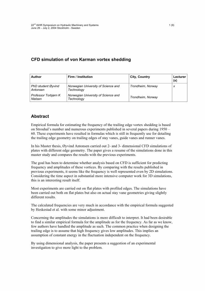
22nd IAHR Symposium on Hydraulic Machinery and Systems 1 (9) June 29 – July 2, 2004 Stockholm - Sweden
CFD simulation of von Karman vortex shedding
Author Firm / Institution City, Country Lecturer (x)
PhD student Øyvind Antonsen
Professor Torbjørn K Nielsen
Norwegian University of Science and Technology
Norwegian University of Science and Technology
Trondheim, Norway
Trondheim, Norway
x
Abstract
Empirical formula for estimating the frequency of the trailing edge vortex shedding is based on Strouhal’s number and numerous experiments published in several papers during 1950 – 60. These experiments have resulted in formulas which is still in frequently use for detailing the trailing edge geometry on trailing edges of stay vanes, guide vanes and runner vanes.
In his Master thesis, Øyvind Antonsen carried out 2- and 3- dimensional CFD simulations of plates with different edge geometry. The paper gives a resume of the simulations done in this master study and compares the results with the previous experiments.
The goal has been to determine whether analysis based on CFD is sufficient for predicting frequency and amplitudes of these vortices. By comparing with the results published in previous experiments, it seems like the frequency is well represented even by 2D simulations. Considering the time aspect in substantial more intensive computer work for 3D simulations, this is an interesting result itself.
Most experiments are carried out on flat plates with profiled edges. The simulations have been carried out both on flat plates but also on actual stay vane geometries giving slightly different results.
The calculated frequencies are very much in accordance with the empirical formula suggested by Heskestad et al. with some minor adjustment.
Concerning the amplitudes the simulations is more difficult to interpret. It had been desirable to find a similar empirical formula for the amplitude as for the frequency. As far as we know, few authors have handled the amplitude as such. The common practice when designing the trailing edge is to assume that high frequency gives low amplitudes. This implies an assumption of constant energy in the fluctuation independent on the frequency.
By using dimensional analysis, the paper presents a suggestion of an experimental investigation to give more light to the problem.

22nd IAHR Symposium on Hydraulic Machinery and Systems 2 (9) June 29 – July 2, 2004 Stockholm - Sweden
Résumé
La formule empirique pour estimer la fréquence de la perte de vortex de rebord arrière est basée sur le nombre de Strouhals et sur de nombreuses expériences édités en plusieurs journal pendant 1950 - 60. Ces expériences ont eu comme conséquence les formules qui est toujours dedans fréquemment utilisation pour détailler la géométrie de rebord arrière sur les rebords arrière des aubes fixes, des aubes direchaices des la roue aubes.
Le but a été de déterminer si l'analyse basée sur le CFD est suffisante pour la fréquence et les amplitudes de prévision de ces vortex. En rivalisant avec les résultats édités dans des expériences précédentes, il semble comme la fréquence est bien représentée même par les 2D simulations.
En ce qui concerne les amplitudes il est plus difficile interpréter les simulations. Il avait été souhaitable de trouver une formule empirique semblable au l'amplitude et à la fréquence. Peu d'auteurs ont manipulé l'amplitude en tant que telle. La pratique courante quand concevoir le rebord arrière doit supposer que la haute fréquence donne de basses amplitudes. Ceci implique une acceptation d'énergie constante dans la fluctuation indépendante sur la fréquence.
Introduction
The occurrence of von Karman vortex train from the outlet edge is a well-known phenomenon and very important to take into consideration when dealing with hydraulic design in general. The classic theory is developed for flow around a cylinder. For hydro turbines, the frequency of the vortex train is possible to determine by empirical formulas with sufficient accuracy.
The pressure amplitude is even more important, but is not that easy to determine. This paper reports CFD calculations of vortex train, which was done during a Master study. The frequencies at various geometries and flow conditions was calculated and fitted very well to the empirical formulas. During this work, we have discussed various approaches to determine the amplitude as well. Dimensional analysis is a good way of enlighten the phenomenon. At this stage, some ideas are presented, and the mentioned CFD calculations indicate that the result of the dimensional analyses might be worthwhile to follow up with experiments.
Theoretical approach
Using dimensional analysis is often an illustrating way of approaching physical phenomena. For flow around a cylindrical object, identifying the properties that the frequency, f, probably is a function of gives:
),,,( UDff µρ= (1)
D – diameter [m] ρ – density [kg/m3] µ – dynamic viscosity [kg/(ms)] U – free stream velocity [m/s]
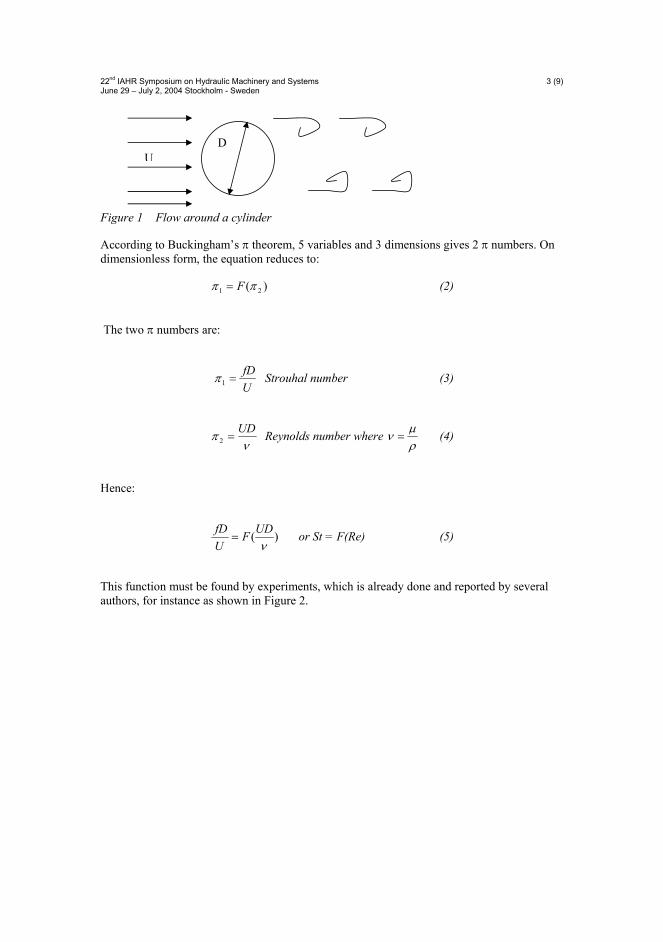
22nd IAHR Symposium on Hydraulic Machinery and Systems 3 (9) June 29 – July 2, 2004 Stockholm - Sweden
Figure 1 Flow around a cylinder
According to Buckingham’s π theorem, 5 variables and 3 dimensions gives 2 π numbers. On dimensionless form, the equation reduces to:
)( 21 ππ F= (2)
The two π numbers are:
UfD
=1π Strouhal number (3)
νπ UD
=2 Reynolds number where ρµν = (4)
Hence:
)(ν
UDFUfD
= or St = F(Re) (5)
This function must be found by experiments, which is already done and reported by several authors, for instance as shown in Figure 2.
D U
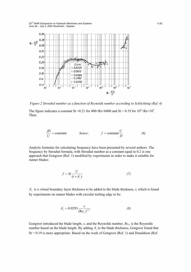
22nd IAHR Symposium on Hydraulic Machinery and Systems 4 (9) June 29 – July 2, 2004 Stockholm - Sweden
Figure 2 Strouhal number as a function of Reynolds number according to Schlichting (Ref. 4)
The figure indicates a constant St =0.21 for 400<Re<6000 and St = 0.19 for 104<Re<105. Then:
constant=UfD hence:
DUf constant= (6)
Analytic formulas for calculating frequency have been presented by several authors. The frequency by Strouhal formula, with Strouhal number as a constant equal to 0.2 is one approach that Gongwer (Ref. 1) modified by experiments in order to make it suitable for runner blades:
)( vt
UStfδ+
= (7)
vδ is a virtual boundary layer thickness to be added to the blade thickness, t, which is found
by experiments on runner blades with circular trailing edge to be:
5/1)(Re0293.0
xv
x=δ (8)
Gongwer introduced the blade length, x, and the Reynolds number, Rex, is the Reynolds number based on the blade length. By adding vδ to the blade thickness, Gongwer found that St = 0.19 is more appropriate. Based on the work of Gongwer (Ref. 1) and Donaldson (Ref.
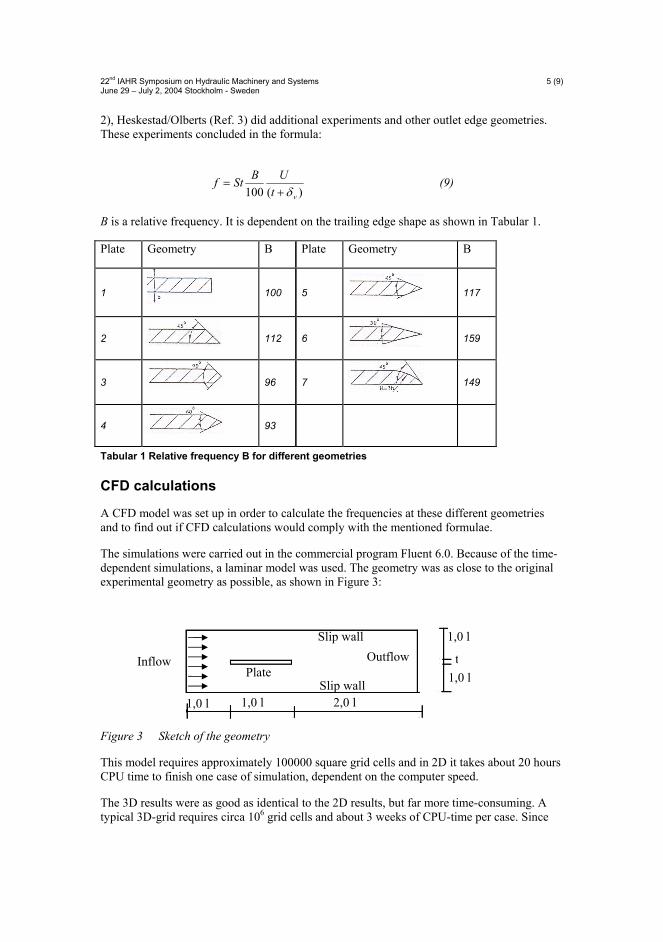
22nd IAHR Symposium on Hydraulic Machinery and Systems 5 (9) June 29 – July 2, 2004 Stockholm - Sweden
2), Heskestad/Olberts (Ref. 3) did additional experiments and other outlet edge geometries. These experiments concluded in the formula:
)(100 vtUBStfδ+
= (9)
B is a relative frequency. It is dependent on the trailing edge shape as shown in Tabular 1.
Plate Geometry B Plate Geometry B
1 100 5 117
2 112 6 159
3 96 7 149
4 93
Tabular 1 Relative frequency B for different geometries
CFD calculations
A CFD model was set up in order to calculate the frequencies at these different geometries and to find out if CFD calculations would comply with the mentioned formulae.
The simulations were carried out in the commercial program Fluent 6.0. Because of the time-dependent simulations, a laminar model was used. The geometry was as close to the original experimental geometry as possible, as shown in Figure 3:
Figure 3 Sketch of the geometry
This model requires approximately 100000 square grid cells and in 2D it takes about 20 hours CPU time to finish one case of simulation, dependent on the computer speed.
The 3D results were as good as identical to the 2D results, but far more time-consuming. A typical 3D-grid requires circa 106 grid cells and about 3 weeks of CPU-time per case. Since
Inflow
Slip wall
1,0 l 1,0 l 2,0 l
1,0 l
Plate Slip wall
Outflow t 1,0 l

22nd IAHR Symposium on Hydraulic Machinery and Systems 6 (9) June 29 – July 2, 2004 Stockholm - Sweden
the results differed negligible, 2D simulations were of course preferred considering the time aspect.
The calculation results were analyzed by examining the oscillating pressure at 18 different points immediate downstream the trailing edge as shown in Figure 4.
Figure 4 Sketch of pressure points.
A perfect match to the frequency deduced by the formula suggested by Heskestad/Olberts was not achieved. A deviation that was only slightly dependent on the parameters in formula (9) was found. The deviation varied with the trailing edge geometry as shown in Tabular 2.
Plate Geometry f_t/f_sim Plate Geometry f_t/f_sim
1 1.15 5 1.23
2 1.36 6 1.18
3 1.27 7 1.21
4 1.10
Tabular 2 The ratio between the empirical calculated and the simulated frequency.
What about the amplitude?
The simulated amplitude values seem to have no connections to the frequency, and the influence of the trailing edge geometry to the amplitude is also difficult to determine. However, for each geometry case the calculated amplitudes seem to be reasonable. The amplitude values are a bit dampened close to the plate, with the highest value in the second point after the trailing edge, and then fading out further downstream, as seen in Figure 5.
Studying the results closely, some interesting facts can be seen. The pressure variation in points 1-6 are in anti-phase to the pressure in points 14-18. This makes sense, considering the alternate shedding from the upper and lower side respectively. The amplitudes have also nearly the same value. The points in the middle will be affected by both the vortices and will therefore have a frequency twice as large as the other points, and amplitude close to zero since the upper and lower vortices will counteract each other. This fact is valid for a symmetric trailing edge only. For an asymmetric trailing edge, the vortices do not shed symmetric on the
1 6
7
13 18
12
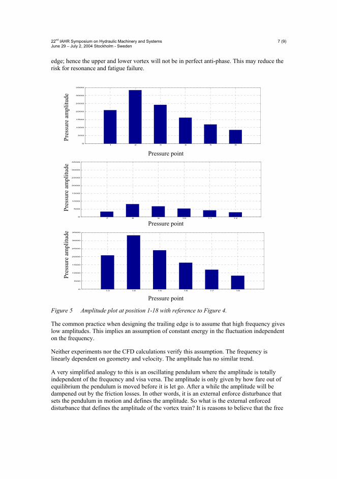
22nd IAHR Symposium on Hydraulic Machinery and Systems 7 (9) June 29 – July 2, 2004 Stockholm - Sweden
edge; hence the upper and lower vortex will not be in perfect anti-phase. This may reduce the risk for resonance and fatigue failure.
Figure 5 Amplitude plot at position 1-18 with reference to Figure 4.
The common practice when designing the trailing edge is to assume that high frequency gives low amplitudes. This implies an assumption of constant energy in the fluctuation independent on the frequency.
Neither experiments nor the CFD calculations verify this assumption. The frequency is linearly dependent on geometry and velocity. The amplitude has no similar trend.
A very simplified analogy to this is an oscillating pendulum where the amplitude is totally independent of the frequency and visa versa. The amplitude is only given by how fare out of equilibrium the pendulum is moved before it is let go. After a while the amplitude will be dampened out by the friction losses. In other words, it is an external enforce disturbance that sets the pendulum in motion and defines the amplitude. So what is the external enforced disturbance that defines the amplitude of the vortex train? It is reasons to believe that the free
1 2 3 4 5 60
500
1000
1500
2000
2500
3000
3500
Pres
sure
am
plitu
de
Pressure point
7 8 9 10 11 120
500
1000
1500
2000
2500
3000
3500
Pres
sure
am
plitu
de
Pressure point
13 14 15 16 17 180
500
1000
1500
2000
2500
3000
3500
Pressure point
Pres
sure
am
plitu
de

22nd IAHR Symposium on Hydraulic Machinery and Systems 8 (9) June 29 – July 2, 2004 Stockholm - Sweden
stream velocity, U, plays an important role. Using a dimensional analysis again might give a certain understanding.
For flow around a cylinder with diameter D, it might be assumed that the amplitude, which must be understood as the pressure amplitude, is a function of frequency, diameter, density, dynamic viscosity and velocity:
),,,,( UDfFp µρ=∆ (10)
There are 6 - 3=3 π-groups to be identified. We already have the Reynolds number and the Strouhal number.
The dimension of the pressure amplitude is N/m2 or kgm/s2m2. Combining it with the other properties in order to form a dimensionless number a suggestion of the 3rd π-number comes forth:
23 Up
ρπ ∆
= (11)
For steady state flow, this number is often referred to as the pressure number. Here, however, ∆p is a pressure oscillation, not a steady state pressure.
According to Buckingham’s pi-theorem:
),( 213 πππ F= (12)
or:
),(2 StRfUp
e=∆ρ
(13)
Using the common assumption, which is at least partly verified in experiments, that the Strouhal number is a constant within a certain Reynolds number region. The simplest equation then becomes:
)(2 eRfconstUp
⋅=∆ρ
(14)
The CFD calculations, however, shows that the pressure amplitude number is also independent of Re number, hence:
constUp
=∆
2ρ (15)
The results of the CFD calculations are shown in Figure 6 where ∆p is defined as the pressure difference between the two sides of the blades. Because of the lack of quality experimental data in this case, it is hard to say how good the CFD results really are. Experiments that will verify whether this is correct or not are planned to be carried out in the close future.
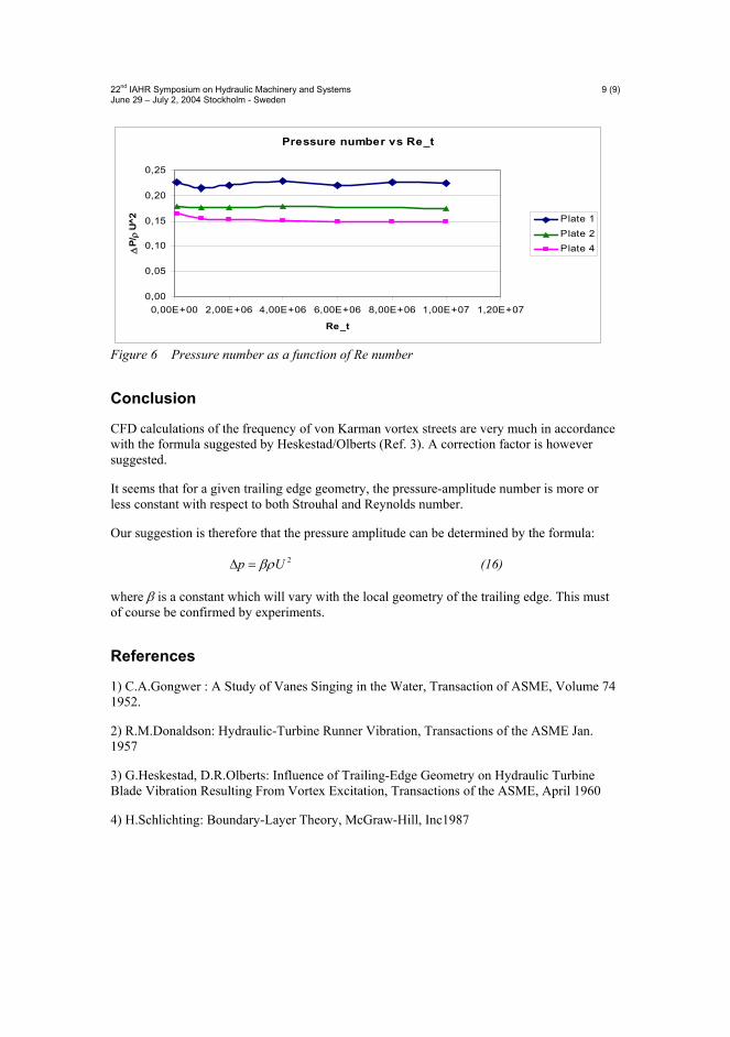
22nd IAHR Symposium on Hydraulic Machinery and Systems 9 (9) June 29 – July 2, 2004 Stockholm - Sweden
Pressure number vs Re_t
0,00
0,05
0,10
0,15
0,20
0,25
0,00E+00 2,00E+06 4,00E+06 6,00E+06 8,00E+06 1,00E+07 1,20E+07
Re_t
∆P
/ ρU^
2 Plate 1Plate 2Plate 4
Figure 6 Pressure number as a function of Re number
Conclusion
CFD calculations of the frequency of von Karman vortex streets are very much in accordance with the formula suggested by Heskestad/Olberts (Ref. 3). A correction factor is however suggested.
It seems that for a given trailing edge geometry, the pressure-amplitude number is more or less constant with respect to both Strouhal and Reynolds number.
Our suggestion is therefore that the pressure amplitude can be determined by the formula:
2Up βρ=∆ (16)
where β is a constant which will vary with the local geometry of the trailing edge. This must of course be confirmed by experiments.
References
1) C.A.Gongwer : A Study of Vanes Singing in the Water, Transaction of ASME, Volume 74 1952.
2) R.M.Donaldson: Hydraulic-Turbine Runner Vibration, Transactions of the ASME Jan. 1957
3) G.Heskestad, D.R.Olberts: Influence of Trailing-Edge Geometry on Hydraulic Turbine Blade Vibration Resulting From Vortex Excitation, Transactions of the ASME, April 1960
4) H.Schlichting: Boundary-Layer Theory, McGraw-Hill, Inc1987

XII Appendix A. Papers
A.2 Hydrovision Portland, Oregon, USA, 2006
Experimental and theoretical investigations of the flow field at the inlet of a Francis runner
By Øyvind Antonsen, Torbjørn K Nielsen and Ole G Dahlhaug. Norwegian University of Science and Technology
Abstract This paper presents and discusses CFD simulations performed in order to investigate the dynamic load inflicted to the runner blade by the outflow from stay vane and wicket gate. The CFD simulations are compared to the results from laboratory experiments in a blade cascade. LDV-measurements of velocity distribution in a cascade for various guide vane profiles were carried out. Later, pressure pulsations in a model turbine where the different guide vane profiles were implemented, was investigated. This is not treated in this paper. For the experiments, a special test rig witch is a 1:2.5 scaled homologous model of the last quarter of a high head Francis turbine, including 5 stay vanes and 5 guide vanes, was used. The velocity profile between the guide vanes were measured by LDV. An overall goal of this project is to improve the accuracy of the theoretical predictions of the dynamic pressure fluctuations at the boundary between the distributor and the runner. A better prediction of the oscillating forces on the blade is essential in order to secure structural safety. Preface The trend towards higher speed and higher output has increased the potential for fluid/structure interaction problems, and the severity of those problems. Under certain conditions these interaction phenomena can lead to structural failure. Turbine manufactures have in recent years experienced several serious runner blade cracking due to high dynamic stress level at runner inlet. The main source of instability at the bounder between distributor and runner is the wake flow from the guide vanes that is chopped by the runner blades, causing oscillating forces. Therefore, an improved prediction of these dynamic forces would be of great value in order to avoid fatigue problems on the runner in the future. In order to investigate this phenomenon a series of laboratory experiments and CFD-calculations has been performed. The experiments where carried out at the Waterpower Laboratory at the Norwegian University of Science and Technology (NTNU).
1
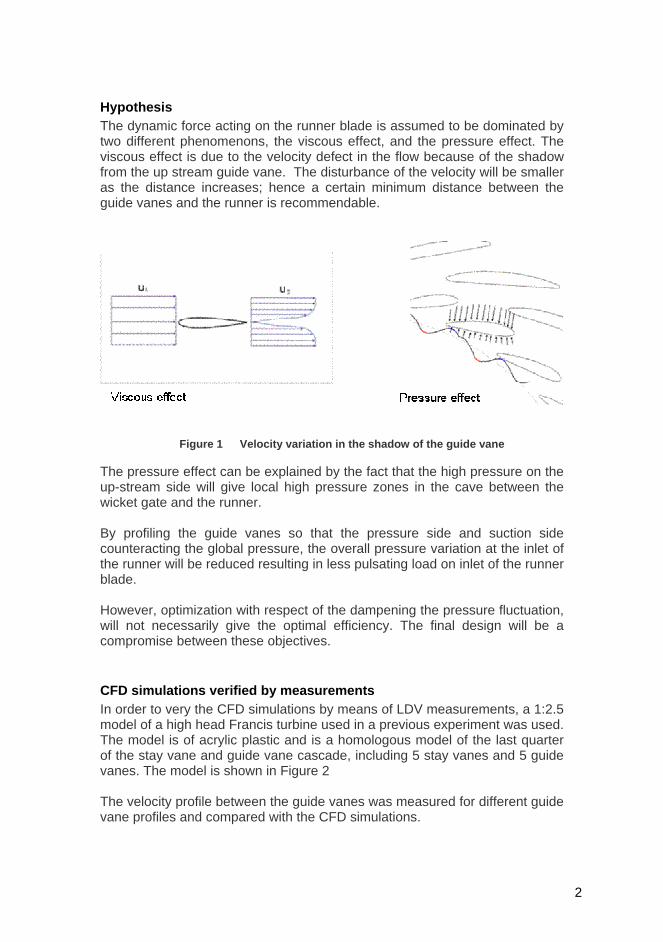
Hypothesis The dynamic force acting on the runner blade is assumed to be dominated by two different phenomenons, the viscous effect, and the pressure effect. The viscous effect is due to the velocity defect in the flow because of the shadow from the up stream guide vane. The disturbance of the velocity will be smaller as the distance increases; hence a certain minimum distance between the guide vanes and the runner is recommendable.
Figure 1 Velocity variation in the shadow of the guide vane
The pressure effect can be explained by the fact that the high pressure on the up-stream side will give local high pressure zones in the cave between the wicket gate and the runner. By profiling the guide vanes so that the pressure side and suction side counteracting the global pressure, the overall pressure variation at the inlet of the runner will be reduced resulting in less pulsating load on inlet of the runner blade. However, optimization with respect of the dampening the pressure fluctuation, will not necessarily give the optimal efficiency. The final design will be a compromise between these objectives. CFD simulations verified by measurements In order to very the CFD simulations by means of LDV measurements, a 1:2.5 model of a high head Francis turbine used in a previous experiment was used. The model is of acrylic plastic and is a homologous model of the last quarter of the stay vane and guide vane cascade, including 5 stay vanes and 5 guide vanes. The model is shown in Figure 2 The velocity profile between the guide vanes was measured for different guide vane profiles and compared with the CFD simulations.
2
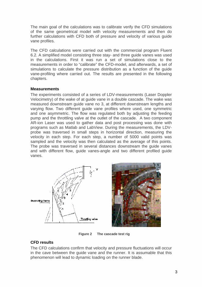
The main goal of the calculations was to calibrate verify the CFD simulations of the same geometrical model with velocity measurements and then do further calculations with CFD both of pressure and velocity of various guide vane profiles. The CFD calculations were carried out with the commercial program Fluent 6.2. A simplified model consisting three stay- and three guide vanes was used in the calculations. First it was run a set of simulations close to the measurements in order to “calibrate” the CFD-model, and afterwards, a set of simulations to calculate the pressure distribution as a function of the guide vane-profiling where carried out. The results are presented in the following chapters. Measurements The experiments consisted of a series of LDV-measurements (Laser Doppler Velocimetry) of the wake of at guide vane in a double cascade. The wake was measured downstream guide vane no 3, at different downstream lengths and varying flow. Two different guide vane profiles where used, one symmetric and one asymmetric. The flow was regulated both by adjusting the feeding pump and the throttling valve at the outlet of the cascade. A two component AR-ion Laser was used to gather data and post processing was done with programs such as Matlab and LabView. During the measurements, the LDV-probe was traversed in small steps in horizontal direction, measuring the velocity in each step. For each step, a number of 5000 valid points was sampled and the velocity was then calculated as the average of this points. The probe was traversed in several distances downstream the guide vanes and with different flow, guide vanes-angle and two different profiled guide vanes.
Figure 2 The cascade test rig
CFD results The CFD calculations confirm that velocity and pressure fluctuations will occur in the cave between the guide vane and the runner. It is assumable that this phenomenon will lead to dynamic loading on the runner blade.
3
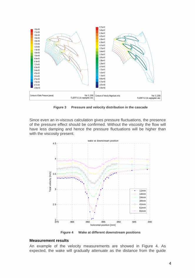
Figure 3 Pressure and velocity distribution in the cascade
Since even an in-viscous calculation gives pressure fluctuations, the presence of the pressure effect should be confirmed. Without the viscosity the flow will have less damping and hence the pressure fluctuations will be higher than with the viscosity present.
-970 -965 -960 -955 -950 -945 -9402
2.5
3
3.5
4
4.5
horizontal position [mm]
Tota
l vel
ocity
[m/s
]
wake vs downstream position
11mm14mm24mm34mm41mm61mm81mm
Figure 4 Wake at different downstream positions
Measurement results An example of the velocity measurements are showed in Figure 4. As expected, the wake will gradually attenuate as the distance from the guide
4
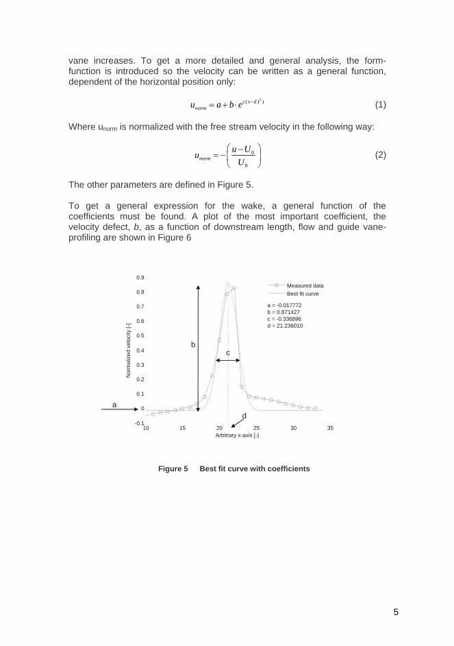
vane increases. To get a more detailed and general analysis, the form-function is introduced so the velocity can be written as a general function, dependent of the horizontal position only:
(1) 2( ) )c x d
normu a b e −= + ⋅
Where unorm is normalized with the free stream velocity in the following way:
0
0norm
u UuU
⎛ ⎞−= −⎜
⎝ ⎠⎟ (2)
The other parameters are defined in Figure 5. To get a general expression for the wake, a general function of the coefficients must be found. A plot of the most important coefficient, the velocity defect, b, as a function of downstream length, flow and guide vane-profiling are shown in Figure 6
10 15 20 25 30 35-0.1
0
0.1
0.2
0.3
0.4
0.5
0.6
0.7
0.8
0.9
Arbitrary x-axis [-]
Nor
mal
ized
vel
ocity
[-]
Measured dataBest fit curve
a = -0.017772b = 0.871427c = -0.336896d = 21.236010
a
bc
d
Figure 5 Best fit curve with coefficients
5
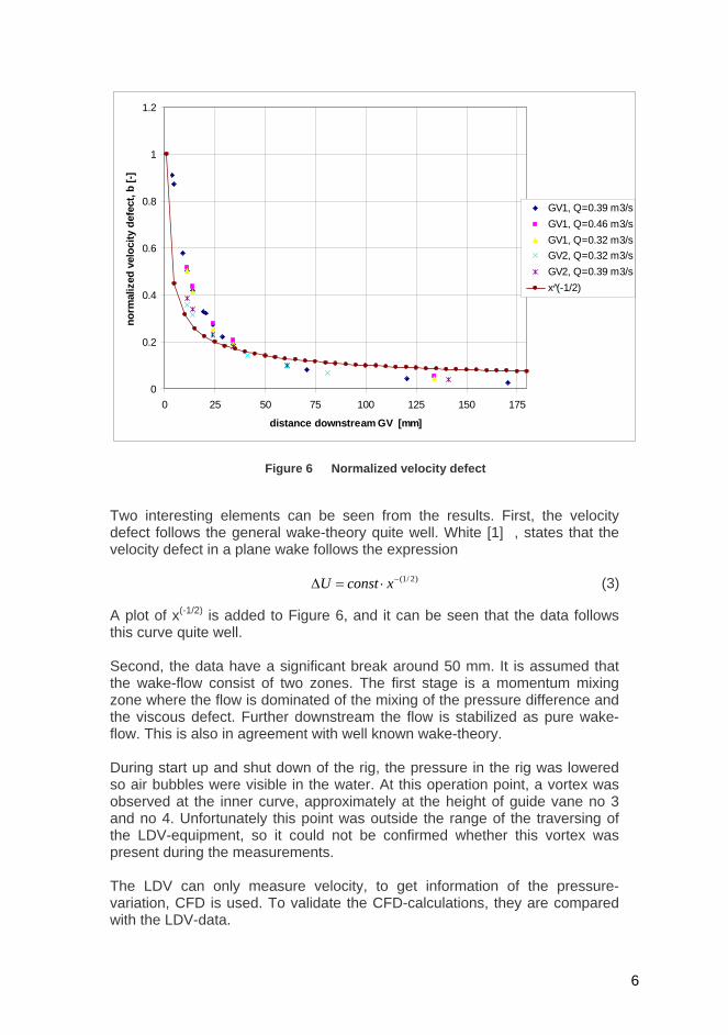
0
0.2
0.4
0.6
0.8
1
1.2
0 25 50 75 100 125 150 175
distance downstream GV [mm]
norm
aliz
ed v
eloc
ity d
efec
t, b
[-]
GV1, Q=0.39 m3/sGV1, Q=0.46 m3/sGV1, Q=0.32 m3/sGV2, Q=0.32 m3/sGV2, Q=0.39 m3/sx (-1/2)
Figure 6 Normalized velocity defect
Two interesting elements can be seen from the results. First, the velocity defect follows the general wake-theory quite well. White [1] , states that the velocity defect in a plane wake follows the expression
(3) (1/ 2)U const x−∆ = ⋅
A plot of x(-1/2) is added to Figure 6, and it can be seen that the data follows this curve quite well. Second, the data have a significant break around 50 mm. It is assumed that the wake-flow consist of two zones. The first stage is a momentum mixing zone where the flow is dominated of the mixing of the pressure difference and the viscous defect. Further downstream the flow is stabilized as pure wake-flow. This is also in agreement with well known wake-theory. During start up and shut down of the rig, the pressure in the rig was lowered so air bubbles were visible in the water. At this operation point, a vortex was observed at the inner curve, approximately at the height of guide vane no 3 and no 4. Unfortunately this point was outside the range of the traversing of the LDV-equipment, so it could not be confirmed whether this vortex was present during the measurements. The LDV can only measure velocity, to get information of the pressure-variation, CFD is used. To validate the CFD-calculations, they are compared with the LDV-data.
6
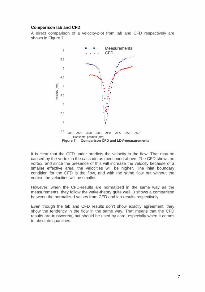
Comparison lab and CFD A direct comparison of a velocity-plot from lab and CFD respectively are shown in Figure 7
-980 -975 -970 -965 -960 -955 -950 -9451.5
2
2.5
3
3.5
4
4.5
5
5.5
6
Horisontal position [mm]
velo
city
[m/s
]
MeasurementsCFD
Figure 7 Comparison CFD and LDV-measurements
It is clear that the CFD under predicts the velocity in the flow. That may be caused by the vortex in the cascade as mentioned above. The CFD shows no vortex, and since the presence of this will increase the velocity because of a smaller effective area, the velocities will be higher. The inlet boundary condition for the CFD is the flow, and with the same flow but without the vortex, the velocities will be smaller. However; when the CFD-results are normalized in the same way as the measurements, they follow the wake-theory quite well. 0 shows a comparison between the normalized values from CFD and lab-results respectively. Even though the lab and CFD results don’t show exactly agreement, they show the tendency in the flow in the same way. That means that the CFD results are trustworthy, but should be used by care, especially when it comes to absolute quantities.
7
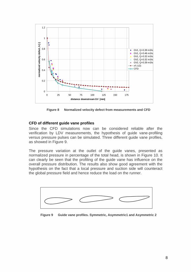
0
0.2
0.4
0.6
0.8
1
1.2
0 25 50 75 100 125 150 175
distance downstream GV [mm]
norm
aliz
ed v
eloc
ity d
efec
t, b
[-]
GV1, Q=0.39 m3/sGV1, Q=0.46 m3/sGV1, Q=0.32 m3/sGV2, Q=0.32 m3/sGV2, Q=0.39 m3/sx (-1/2)CFD
Figure 8 Normalized velocity defect from measurements and CFD
CFD of different guide vane profiles Since the CFD simulations now can be considered reliable after the verification by LDV measurements, the hypothesis of guide vane-profiling versus pressure pulses can be simulated. Three different guide vane profiles, as showed in Figure 9. The pressure variation at the outlet of the guide vanes, presented as normalized pressure in percentage of the total head, is shown in Figure 10. It can clearly be seen that the profiling of the guide vane has influence on the overall pressure distribution. The results also show good agreement with the hypothesis on the fact that a local pressure and suction side will counteract the global pressure field and hence reduce the load on the runner.
Figure 9 Guide vane profiles. Symmetric, Asymmetric1 and Asymmetric 2
8
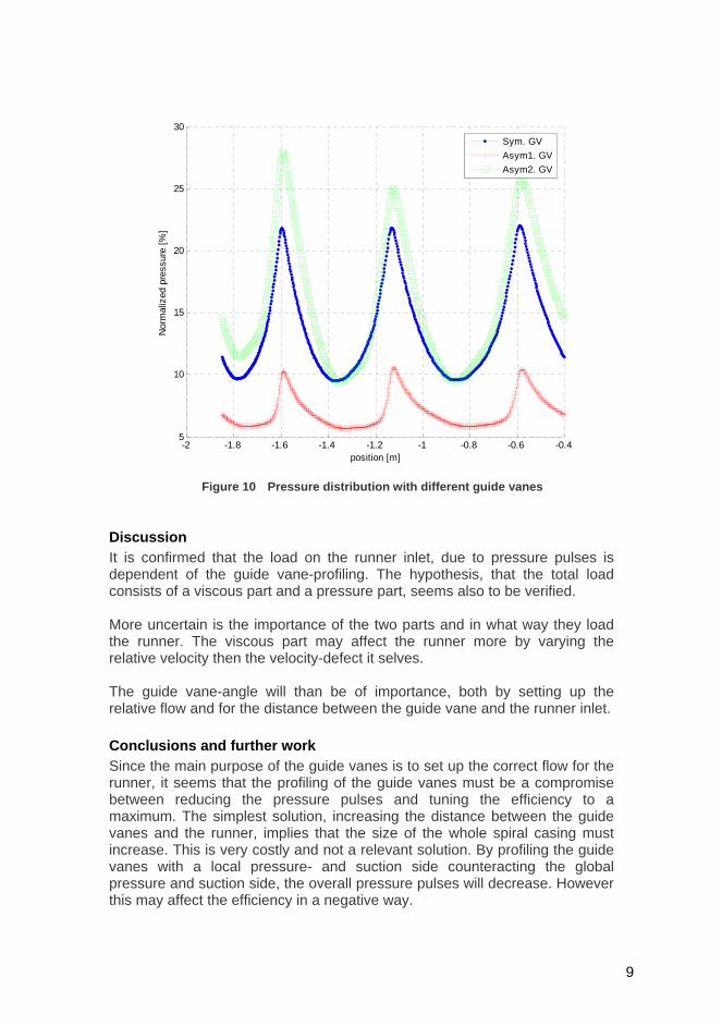
-2 -1.8 -1.6 -1.4 -1.2 -1 -0.8 -0.6 -0.45
10
15
20
25
30
position [m]
Nor
mal
ized
pre
ssur
e [%
]
Sym. GVAsym1. GVAsym2. GV
Figure 10 Pressure distribution with different guide vanes
Discussion It is confirmed that the load on the runner inlet, due to pressure pulses is dependent of the guide vane-profiling. The hypothesis, that the total load consists of a viscous part and a pressure part, seems also to be verified. More uncertain is the importance of the two parts and in what way they load the runner. The viscous part may affect the runner more by varying the relative velocity then the velocity-defect it selves. The guide vane-angle will than be of importance, both by setting up the relative flow and for the distance between the guide vane and the runner inlet. Conclusions and further work Since the main purpose of the guide vanes is to set up the correct flow for the runner, it seems that the profiling of the guide vanes must be a compromise between reducing the pressure pulses and tuning the efficiency to a maximum. The simplest solution, increasing the distance between the guide vanes and the runner, implies that the size of the whole spiral casing must increase. This is very costly and not a relevant solution. By profiling the guide vanes with a local pressure- and suction side counteracting the global pressure and suction side, the overall pressure pulses will decrease. However this may affect the efficiency in a negative way.
9

To further investigate the relations between guide vanes-profiling, pressure pulses and efficiency there is ongoing work right now. Pressure pulses and efficiency are measured in a model turbine with the same guide vanes -profiles as used in the LDV-measurements. References [1] White, Frank. Viscous fluid flow. McGraw-Hill. 1991 Aknowlegdement The authors wish to thank Morten Kjeldsen for his support during the work of this paper. Authors Øyvind Antonsen is PhD-student at the water power lab at the Norwegian University of Science and Technology (NUST). His work includes general pressure pulses in Francis turbines and unsteady load at the inlet of the runner in particular. Torbjørn K. Nielsen is a professor at Norwegian University of Science and Technology, NTNU, since 2002. His main topic is hydraulic machinery, including the responsibility for The Waterpower Laboratory. Ole Gunnar Dahlhaug is an associate professor at the Waterpower Laboratory at Norwegian University of Science and Technology, NTNU, since 1999. His main topic is design, maintenance and development of hydraulic machinery.
10

A.3. IAHR Yokohama Japan, 2006 XXIII
A.3 IAHR Yokohama Japan, 2006
23rd IAHR Symposium - Yokohama October 2006
1 (7)
Pressure Pulses in Francis Turbines vs. Guide Vane Design Øyvind ANTONSEN* Norwegian University of Science and Technology (NTNU)
[email protected] Torbjørn K. NIELSEN NTNU [email protected] Ole G. DAHLHAUG NTNU [email protected] Jan T.BILLDAL GE Energy [email protected] Key words: Pressure pulses, Francis turbine, Guide vane design.
Abstract In order to investigate the pressure pulses at the inlet of a Francis runner, unsteady pressure measurements are carried out in the volute region between the outlet of the guide vanes and the inlet of the runner in a model turbine. The results show that the dominant pulse in this area is the blade passing frequency. By removing the splitter blades on the runner or adding end sealing on the guide vanes, the pressure pulses was changed and gave higher pressure pulses, while smaller changes on the guide vanes or stay vanes did not affect the results.
Introduction Vibrations at the inlet of a Francis turbine runner caused by the interaction between the runner and the guide vanes are a well known phenomenon. However it is still experienced problems with high sound level and runner blade cracking due to this kind of vibrations. The trend with more kW power per kg turbine also makes the turbines more vulnerable for damage due to vibrations. The flow in the volute region between the outlet of the guide vanes and the inlet of the runner has a complex flow field, consists of vortex gates from the guide vanes, horseshoe vortices at the upper and lower cover due to the boundary layer and pressure variations over the guide vanes, leakage flow between the guide vanes and upper and lower cover, pressure difference over the guide vanes, both due to the accelerated flow and the profiling of the guide vanes and finally the influence of a rotating runner. All these factors will influence on the total pressure load on the runner, but in different extent depending on the design of the turbine. In order to dig deeper into this field, a PhD-study has carried out at the Water Power Lab at the Norwegian University of Science and Technology. The study consists of a part with LDA-measurements of the wake of different guide vane profiles and a part with unsteady pressure measurements in the volute region between the outlet of the guide vanes and the inlet of the runner. The results from the LDA measurements are presented in a paper to the Hydrovision 2006, Portland (Ref 1). This paper will focus on the results from the unsteady pressure measurements.
23rd IAHR Symposium - Yokohama October 2006
2 (7)
Theory In the volute region between the outlet of the guide vanes and inlet of the runner, the influence on the flow field is mainly governed by the guide vane wakes and the rotating runner blades. The runner blades will rotate through a non uniform velocity- and pressure field, due to the wake of the guide vanes, causing pressure pulses on the runner blades. Chen (Ref 2) measured the velocity profile at the inlet of the runner and concluded that the velocity profile is neither uniform in circumferential nor in the span wise direction. Hence, the presence of guide vanes in the flow will disturb the flow and set up a non uniform flow field in which the runner blades rotate. This will cause a varying load on the runner blades, dependent of the flow, profile of the guide vanes, the distance between the guide vanes and the runner and the rotational speed of the runner. At the outlet of the guide vanes, the pressure field is non-uniform both due to the acceleration of the flow and due to the local pressure and suction side of the guide vanes. It is assumed that by profiling the guide vanes with pressure and suction sides that counteracts the global pressure variation, the overall load on the runner blades will be reduced. LDA measurements and CFD-calculations by Antonsen et al. (Ref 1) confirm that the pressure variations will be smaller with the right profiling of the guide vanes. Experiments by Jernsletten, (Ref 3), also confirm the guide vanes influence on the runner blades. By measure the load on the runner blades before and after cutting the inlet of the runner, the load on the runner was reduced with 1/3 by increasing the radial distance with 5.1 mm. The runner blades will also create a change in the flow field due to its rotation. A stationary point will sense a change in pressure each time a runner blade passes the point. This change of pressure causes pressure waves which are propagating around the circumference. When designing turbines, it is important to choose the number of guide vanes and runner vanes carefully to avoid amplifying and resonance of this pressure wave. It is desirable that as few runner blades hits a wake at the same time. It is also important that the wave don’t propagate to the next wake at the same time as a runner blade hits the wake and so build up a larger wave. Lund, (Ref 4), described the pressure wave’s propagation by a range of Fourier series. Hence, combinations of favorable and unfavorable numbers of guide vanes and runner blades could be calculated.
Experiment The measurements were carried out on a model of a high head Francis turbine with 23 stay vanes, 23 guide vanes, and a runner with 15 blades, and 15 splitter blades. Three piezoelectric pressure transducers were mounted flush with the lower cover between the outlet of the guide vanes, and the inlet of the runner, see Figure 1. These transducers only measure changes in pressure, but is excellent for finding frequency and amplitude in such measurements due to their small size and fast response. For some test series one of the transducers was placed in the draft tube cone in order to
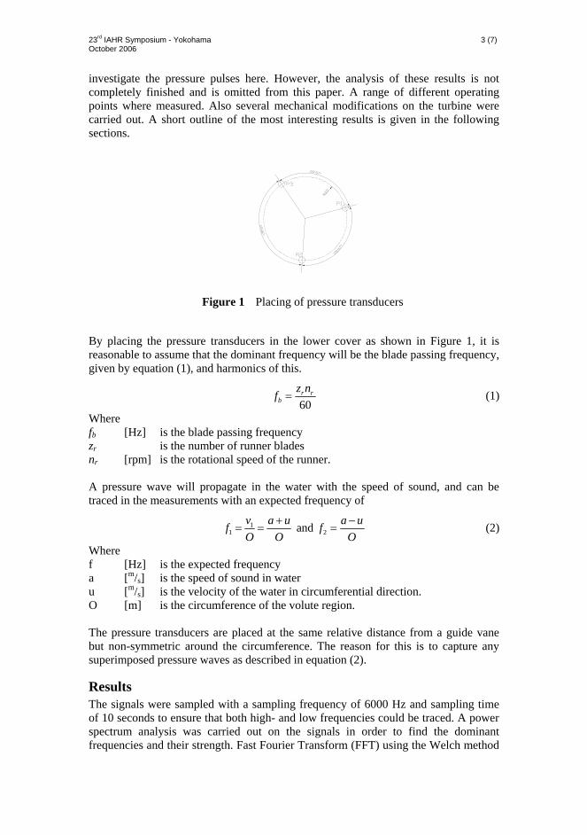
23rd IAHR Symposium - Yokohama October 2006
3 (7)
investigate the pressure pulses here. However, the analysis of these results is not completely finished and is omitted from this paper. A range of different operating points where measured. Also several mechanical modifications on the turbine were carried out. A short outline of the most interesting results is given in the following sections.
Figure 1 Placing of pressure transducers
By placing the pressure transducers in the lower cover as shown in Figure 1, it is reasonable to assume that the dominant frequency will be the blade passing frequency, given by equation (1), and harmonics of this.
60r r
bz nf = (1)
Where fb [Hz] is the blade passing frequency zr is the number of runner blades nr [rpm] is the rotational speed of the runner. A pressure wave will propagate in the water with the speed of sound, and can be traced in the measurements with an expected frequency of
11 2 and v a u a uf f
O O O+ −
= = = (2)
Where f [Hz] is the expected frequency a [m/s] is the speed of sound in water u [m/s] is the velocity of the water in circumferential direction. O [m] is the circumference of the volute region. The pressure transducers are placed at the same relative distance from a guide vane but non-symmetric around the circumference. The reason for this is to capture any superimposed pressure waves as described in equation (2).
Results The signals were sampled with a sampling frequency of 6000 Hz and sampling time of 10 seconds to ensure that both high- and low frequencies could be traced. A power spectrum analysis was carried out on the signals in order to find the dominant frequencies and their strength. Fast Fourier Transform (FFT) using the Welch method
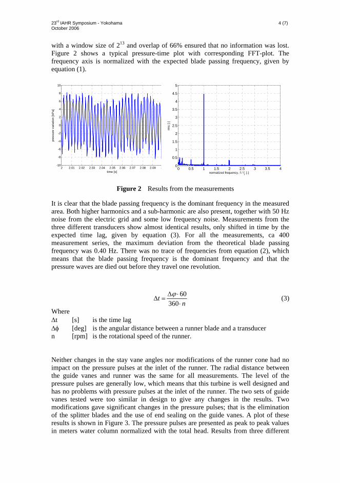
23rd IAHR Symposium - Yokohama October 2006
4 (7)
with a window size of 213 and overlap of 66% ensured that no information was lost. Figure 2 shows a typical pressure-time plot with corresponding FFT-plot. The frequency axis is normalized with the expected blade passing frequency, given by equation (1).
Figure 2 Results from the measurements
It is clear that the blade passing frequency is the dominant frequency in the measured area. Both higher harmonics and a sub-harmonic are also present, together with 50 Hz noise from the electric grid and some low frequency noise. Measurements from the three different transducers show almost identical results, only shifted in time by the expected time lag, given by equation (3). For all the measurements, ca 400 measurement series, the maximum deviation from the theoretical blade passing frequency was 0.40 Hz. There was no trace of frequencies from equation (2), which means that the blade passing frequency is the dominant frequency and that the pressure waves are died out before they travel one revolution.
60360
tn
ϕΔ ⋅Δ =
⋅ (3)
Where Δt [s] is the time lag Δφ [deg] is the angular distance between a runner blade and a transducer n [rpm] is the rotational speed of the runner. Neither changes in the stay vane angles nor modifications of the runner cone had no impact on the pressure pulses at the inlet of the runner. The radial distance between the guide vanes and runner was the same for all measurements. The level of the pressure pulses are generally low, which means that this turbine is well designed and has no problems with pressure pulses at the inlet of the runner. The two sets of guide vanes tested were too similar in design to give any changes in the results. Two modifications gave significant changes in the pressure pulses; that is the elimination of the splitter blades and the use of end sealing on the guide vanes. A plot of these results is shown in Figure 3. The pressure pulses are presented as peak to peak values in meters water column normalized with the total head. Results from three different
2 2.01 2.02 2.03 2.04 2.05 2.06 2.07 2.08 2.09 2.1-10
-8
-6
-4
-2
0
2
4
6
8
10
pres
sure
var
iatio
n [k
Pa]
time [s]0 0.5 1 1.5 2 2.5 3 3.5 4
0
0.5
1
1.5
2
2.5
3
3.5
4
4.5
5
normalized frequency, f / fr [-]rm
s [-]
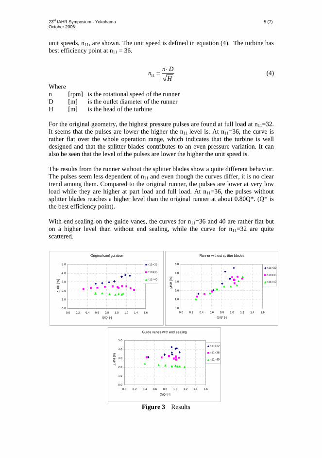
23rd IAHR Symposium - Yokohama October 2006
5 (7)
unit speeds, n11, are shown. The unit speed is defined in equation (4). The turbine has best efficiency point at n11 = 36.
11n Dn
H⋅
= (4)
Where n [rpm] is the rotational speed of the runner D [m] is the outlet diameter of the runner H [m] is the head of the turbine For the original geometry, the highest pressure pulses are found at full load at n11=32. It seems that the pulses are lower the higher the n11 level is. At n11=36, the curve is rather flat over the whole operation range, which indicates that the turbine is well designed and that the splitter blades contributes to an even pressure variation. It can also be seen that the level of the pulses are lower the higher the unit speed is. The results from the runner without the splitter blades show a quite different behavior. The pulses seem less dependent of n11 and even though the curves differ, it is no clear trend among them. Compared to the original runner, the pulses are lower at very low load while they are higher at part load and full load. At n11=36, the pulses without splitter blades reaches a higher level than the original runner at about 0.80Q*. (Q* is the best efficiency point). With end sealing on the guide vanes, the curves for n11=36 and 40 are rather flat but on a higher level than without end sealing, while the curve for n11=32 are quite scattered.
Figure 3 Results
Original configuration
0.0
1.0
2.0
3.0
4.0
5.0
0.0 0.2 0.4 0.6 0.8 1.0 1.2 1.4 1.6
Q/Q* [-]
ΔH/H
[%]
n11=32
n11=36
n11=40
Runner without splitter blades
0.0
1.0
2.0
3.0
4.0
5.0
0.0 0.2 0.4 0.6 0.8 1.0 1.2 1.4 1.6
Q/Q* [-]
ΔH
/H [%
]
n11=32
n11=36
n11=40
Guide vanes with end sealing
0.0
1.0
2.0
3.0
4.0
5.0
0.0 0.2 0.4 0.6 0.8 1.0 1.2 1.4 1.6
Q/Q* [-]
ΔH
/H [%
]
n11=32
n11=36
n11=40
23rd IAHR Symposium - Yokohama October 2006
6 (7)
One noteworthy fact is the increase of pressure pulses with the added end sealing on the guide vanes. The end sealing will reduce the clearance flow between the guide vanes and the upper and lower cover. This will give less disturbance of the main flow field and hence higher efficiency of the turbine. However, this clearance flow might contribute to a faster mixing of the guide vane wake and hence reduce the pressure pulses on the runner. By removing the splitter blades on the runner, the best efficiency point of the turbine was shifted towards higher n11. Hence the curve for n11=40 in Figure 3 is closer to the best efficiency point than the n11=36 curve. Without the splitter blades the pressure variation between suction side and pressure side of the runner blades are bigger than with splitter blades. With a bigger pressure difference rotating with the runner, it is reasonable that the pressure pulses are higher for this case. Since this turbine generally has low pressure pulses and since it needed quite large modifications before any change in the pressure pulses occurred it might not be the best model to find trends in the pressure pulses. However it is no doubt that at the inlet of the runner it is the blade passing frequency that is the dominant factor.
Conclusions Unsteady pressure measurements in a model of a high head Francis turbine have been carried out. The results show that at the inlet of a Francis runner, the pressure pulses are dominated by the blade passing frequency. For this turbine the level of pressure pulses was rather low over the whole operation area. This is according to the expected results since the guide vanes are slightly asymmetric profiled with a pressure side counteracting the pressure field set up by the accelerating flow. This gives a quite uniform pressure field for the runner blades to rotate in and hence a low level on the pressure pulses. By adding end sealing on the guide vanes, it will be less mixing of the guide vane wake and this will contribute to a higher level of pressure pulses. By removing the splitter blades, the pressure difference between the suction side and the pressure side of the runner will increase and hence the pressure pulses will increase. Unfortunately the difference in the two sets of guide vanes was not big enough to give any changes in the pressure pulses. In order to further confirm the hypothesis and to investigate the flow field at the inlet of the runner, CFD-calculations and further analysis of the measurement data will be carried out.

23rd IAHR Symposium - Yokohama October 2006
7 (7)
References (Ref 1) Antonsen, Nielsen and Dahlhaug. Experimental and theoretical
investigations of the flow field at the inlet of a Francis runner. Hydrovision 2006, Portland Oregon.
(Ref 2) Xin Chen. Theoretical and experimental study of flow through the double
cascade of a Francis turbine. PhD-thesis. Norwegian Institute of Technology. 1992.
(Ref 3) Jernsletten, Jo. Analysis of non-stationary flow in a Francis reversible pump
turbine runner. PhD-thesis. Norwegian Institute of Technology. 1995. (Ref 4) Lund, Emil. Hydrauliske trykksvingninger i omdreiningshulrommet mellom
løpehjul og ledeapparat i en Francis turbin. (in Norwegian). Lisentiatarbeid, Norwegian Institute of Technology. 1966