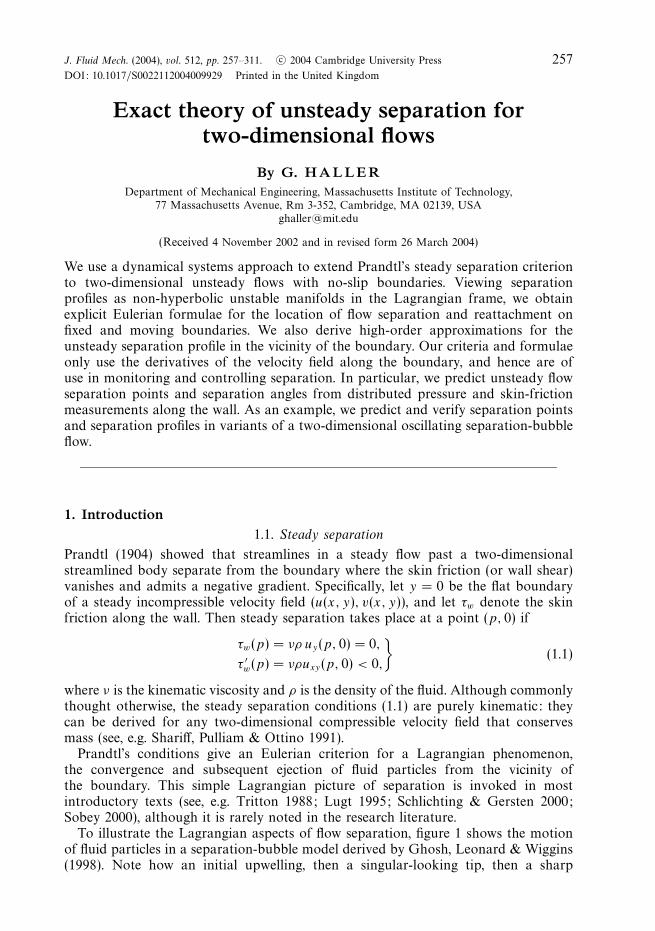
J. Fluid Mech. (2004), vol. 512, pp. 257–311. c© 2004 Cambridge University Press

DOI: 10.1017/S0022112004009929 Printed in the United Kingdom

257

Exact theory of unsteady separation fortwo-dimensional flows

By G. HALLERDepartment of Mechanical Engineering, Massachusetts Institute of Technology,

77 Massachusetts Avenue, Rm 3-352, Cambridge, MA 02139, USAghaller@mit.edu

(Received 4 November 2002 and in revised form 26 March 2004)

We use a dynamical systems approach to extend Prandtl’s steady separation criterionto two-dimensional unsteady flows with no-slip boundaries. Viewing separationprofiles as non-hyperbolic unstable manifolds in the Lagrangian frame, we obtainexplicit Eulerian formulae for the location of flow separation and reattachment onfixed and moving boundaries. We also derive high-order approximations for theunsteady separation profile in the vicinity of the boundary. Our criteria and formulaeonly use the derivatives of the velocity field along the boundary, and hence are ofuse in monitoring and controlling separation. In particular, we predict unsteady flowseparation points and separation angles from distributed pressure and skin-frictionmeasurements along the wall. As an example, we predict and verify separation pointsand separation profiles in variants of a two-dimensional oscillating separation-bubbleflow.

1. Introduction1.1. Steady separation

Prandtl (1904) showed that streamlines in a steady flow past a two-dimensionalstreamlined body separate from the boundary where the skin friction (or wall shear)vanishes and admits a negative gradient. Specifically, let y = 0 be the flat boundaryof a steady incompressible velocity field (u(x, y), v(x, y)), and let τw denote the skinfriction along the wall. Then steady separation takes place at a point (p, 0) if

τw(p) = νρ uy(p, 0) = 0,

τ ′w(p) = νρuxy(p, 0) < 0,

}(1.1)

where ν is the kinematic viscosity and ρ is the density of the fluid. Although commonlythought otherwise, the steady separation conditions (1.1) are purely kinematic: theycan be derived for any two-dimensional compressible velocity field that conservesmass (see, e.g. Shariff, Pulliam & Ottino 1991).

Prandtl’s conditions give an Eulerian criterion for a Lagrangian phenomenon,the convergence and subsequent ejection of fluid particles from the vicinity ofthe boundary. This simple Lagrangian picture of separation is invoked in mostintroductory texts (see, e.g. Tritton 1988; Lugt 1995; Schlichting & Gersten 2000;Sobey 2000), although it is rarely noted in the research literature.

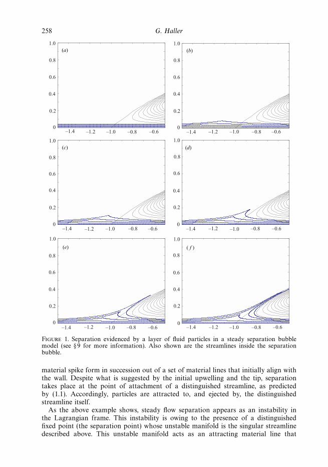
To illustrate the Lagrangian aspects of flow separation, figure 1 shows the motionof fluid particles in a separation-bubble model derived by Ghosh, Leonard & Wiggins(1998). Note how an initial upwelling, then a singular-looking tip, then a sharp

258 G. Haller

–1.4 –1.2 –0.8 –0.6–1.00

1.0

0.8

0.6

0.4

0.2

–1.4 –1.2 –1.0 –0.8 –0.60

0.2

0.4

0.6

0.8

1.0

–1.4 –1.2 –1.0 –0.8 –0.60

0.2

0.4

0.6

0.8

1.0

–1.4 –1.2 –1.0 –0.8 –0.60

1.0

0.8

0.6

0.4

0.2

–1.4 –1.2 –1.0 –0.8 –0.60

0.2

0.4

0.6

0.8

1.0

–1.4 –1.2 –1.0 –0.8 –0.60

1.0

0.8

0.6

0.4

0.2

(a) (b)

( f )(e)

(c) (d)

Figure 1. Separation evidenced by a layer of fluid particles in a steady separation bubblemodel (see § 9 for more information). Also shown are the streamlines inside the separationbubble.

material spike form in succession out of a set of material lines that initially align withthe wall. Despite what is suggested by the initial upwelling and the tip, separationtakes place at the point of attachment of a distinguished streamline, as predictedby (1.1). Accordingly, particles are attracted to, and ejected by, the distinguishedstreamline itself.

As the above example shows, steady flow separation appears as an instability inthe Lagrangian frame. This instability is owing to the presence of a distinguishedfixed point (the separation point) whose unstable manifold is the singular streamlinedescribed above. This unstable manifold acts as an attracting material line that

Exact theory of unsteady separation 259

collects and transports particles away from the wall. The distinguished fixed pointis degenerate owing to the no-slip boundary conditions, and hence its location andstability cannot be predicted from linearization. Prandtl’s first condition in (1.1) givesa necessary condition for the existence of such a degenerate fixed point, while (1.1) asa whole gives a sufficient set of conditions for the existence of an unstable manifold.

1.2. Prior work on unsteady separation

For unsteady velocity fields, the Lagrangian and Eulerian descriptions of separationdiffer. On the Eulerian side, initial suggestions that unsteady flow separation alsotakes place at points of zero skin friction were dismissed by numerical simulationsof boundary-layer separation by Rott (1956), Moore (1958) and Sears & Telionis(1971). Specifically, Sears & Telionis (1975) observed that vanishing wall shear ‘doesnot denote separation in any meaningful sense in unsteady flow’, and proposeda separation criterion that has become known as the Moore–Rott–Sears (MRS)principle.

According to the MRS principle, unsteady separation takes place at a pointoff the boundary where the wall-component of the shear vanishes and the localstreamwise velocity equals the velocity of the moving separation structure. Thispostulate, however, requires the a priori knowledge of the separation speed, makingthe MRS principle difficult, if not impossible, to apply (Williams 1977; Van Dommelen1981).

On the Lagrangian side, Van Dommelen (1981) and Van Dommelen & Shen (1982)initiated the numerical study of unsteady boundary-layer separation in Lagrangiancoordinates. This approach has removed earlier computational difficulties seen in theEulerian frame, and revealed the true Lagrangian signature of unsteady separation.As explained by Cowley, Van Dommelen & Lam (1990), this frame-independentsignature is precisely the one shown in figure 1. The contraction of an infinitesimalfluid element in the streamwise direction is accompanied by a spiky expansion in thewall-normal direction.

Van Dommelen and coworkers attribute the material spike to the formation of asingularity in the boundary-layer equations, and define the unsteady separation pointas the location of the singularity. A number of separation studies have since confirmedthe advantages of Lagrangian coordinates (see, e.g. Peridier 1995; Cassel, Smith &Walker 1996; Degani, Walker & Smith 1998), and formal asymptotic expansions areavailable for Van Dommelen’s singularity in the boundary-layer equations (Cowley1983; Van Dommelen & Cowley 1990). Analytic results show, however, that separationin the boundary-layer equations has no direct connection with velocity singularities(Liu & Wan 1985).

Despite computational advances on boundary-layer separation, a theoreticallysound description has been missing for general unsteady flow separation, aphenomenon that is equally common for high and low Reynolds numbers. As Sears &Telionis (1975) point out, we would ideally need an unsteady separation definitionthat does not depend on our ability to solve the boundary-layer equations accurately.Secondly, as suggested by Cowley et al. (1990), an ideal separation definition shouldbe independent of the coordinate system selected. Thirdly, as argued by Wu et al.(2000), the growing interest in active flow control calls for a separation criterion thatuses quantities measured or computed along the boundary.

The Lagrangian definition of steady separation (reviewed in connection withfigure 1) has the above three ingredients, and hence is an ideal starting pointfor a rigorous unsteady separation theory. Such a theory was first proposed by

260 G. Haller

Shariff et al. (1991) for two-dimensional incompressible time-periodic flows. Shariffet al. defined the separation point as a fixed point with an unstable manifold forthe Poincare map associated with the periodic flow. Using this Lagrangian definition,they showed that unsteady separation points are located at boundary points wherethe time-average of the skin friction vanishes. This remarkable result, however, isbased on an assertion on the Poincare map that has remained unverified ever since.

Realizing the above shortcoming, Yuster & Hackborn (1997) re-derived thezero-mean-friction principle for near-steady time-periodic incompressible flows in amathematically rigorous way; Hackborn, Ulucakli & Yuster (1997) verified the resultexperimentally. The validity of the zero-mean-skin friction principle for general time-periodic flows, however, has remained an open question. As a notable contribution,Yuster & Hackborn (1997) showed that the principle fails for compressible time-periodic flows.

In summary, the only available rigorous unsteady separation criterion has beenthe zero-mean-friction principle, which applies to time-periodic incompressible flowsthat are close to a steady limit. No results have been derived for compressible flows,or for flows with general time dependence. In addition, no rigorous theory has beenproposed for moving separation, which cannot be explained by classical unstablemanifolds (cf. § 8).

1.3. Results on fixed separation

In this paper, we extend the Lagrangian view of separation from steady flows tocompressible unsteady flows with general time dependence. Specifically, we definefixed unsteady flow separation as a material instability induced by an unstablemanifold of a distinguished boundary point. In this general context, the unstablemanifold is a time-dependent material line that shrinks to the separation point inbackward time. In forward time, the unstable manifold attracts and ejects particlesfrom a vicinity of the boundary.

Using the above Lagrangian definition, we derive mathematically exact Euleriancriteria that locate time-dependent unstable manifolds emanating from the wall.Because of the degeneracy (non-hyperbolicity) of fixed points on a no-slip wall,classical dynamical systems methods for locating their unstable manifolds fail toapply. Equally inapplicable are the Poincare-map arguments of Shariff et al. (1991)and Yuster & Hackborn (1997) because of the general time-dependence we allow for.To overcome these limitations of classical invariant manifold theory, we develop anovel nonlinear technique that renders both the location and the shape of unstablemanifolds or separation profiles.

We show that fixed (i.e. non-moving) separation takes place where the weightedbackward-time average of the skin friction remains uniformly bounded. The weightfunction in this average is just the squared reciprocal of the fluid density. We alsoclarify the meaning of effective separation points at which the weighted finite-timemean of the skin friction vanishes. These points turn out to converge to fixedseparation points provided that an unsteady version of Prandtl’s second separationcondition (cf. (1.1)) holds.

When applied to simple flows, our criteria agree with prior exact separationcriteria for such flows. Specifically, for steady flows, our general criteria coincidewith those of Prandtl (1904) and Lighthill (1963). When applied to incompressibletime-periodic flows, our results agree with those of Shariff et al. (1991) and Yuster &Hackborn (1997). Finally, when translated into the Lagrangian frame, our separationcriterion agrees with the second criterion of Van Dommelen (1981) for boundary-layer

Exact theory of unsteady separation 261

separation. Most importantly, however, our kinematic theory predicts unsteady flowseparation in general velocity fields that are inaccessible to previous theories.

1.4. Results on moving separation

By moving separation we mean separation where the separation point may move,disappear and reappear. In such cases, classical invariant manifold theory turns outto be inapplicable; we need to use finite-time unstable manifolds (Haller 2000, 2001) todescribe moving separation profiles. Finite-time unstable manifolds are inherently non-unique, and so are moving separation profiles. The distance between two separationprofiles, however, tends to zero as their time of existence increases (Haller 2000).

We present two approaches to moving separation: a heuristic and a rigorous one.The first approach assumes that the backward-time integral of the skin friction hasa well-defined mean component, or equivalently, that a well-defined mean separationprofile exists in the Lagrangian frame. This assumption leads to a heuristic necessarycriterion that identifies moving separation as a bifurcation in the mean evolution ofwall-bound material lines.

When applied to analytic flow models, the heuristic criterion yields explicitexpressions for the location and shape of the moving separation profile. Whenapplied to numerical or experimental data, the criterion gives separation profiles thatconverge to the moving profile as more and more past velocity data is processed inthe calculation.

Our second method for locating moving separation, a sufficient criterion, is basedon a rigorous analytic construction of finite-time unstable manifolds near effectiveseparation points. Effective separation points depend sensitively on the time scaleover which they are computed, but we find the time scale for which they closelyapproximate a nearby moving separation point. This time scale results from a generalanalytic estimate that may be further strengthened for particular classes of flows.

With the exception of quasi-periodic and periodic flows, most unsteady flowsproduce moving separation, and hence should be analysed by the above two criteria.If the separation happens to be fixed, the heuristic necessary criterion produces movingseparation points that converge to the fixed separation point after initial transients.By contrast, our sufficient criterion yields separation points that are close to the fixedseparation from the start, but this closeness may not improve further in time.

As we illustrate in examples, our moving separation criteria perform reliably underboth regular and stochastic time dependence, suggesting that the separation theorydescribed here is equally applicable to laminar and turbulent flows.

1.5. Organization of the paper

We derive necessary conditions for fixed compressible separation in § 2, and give aquadratic approximation for a general compressible separation profile. Section 2 alsocontains equivalent Lagrangian and density-independent formulations of our criteria,as well as the treatment of moving and non-smooth boundaries. We show how thetheory simplifies for incompressible flows in § 3, and exploit this simplification toderive a quartic-order approximation for incompressible separation profiles.

In § 4, we give a kinetic version of our separation criteria for Navier–Stokes flows,and, in § 5, we formulate sufficient conditions for sharp unsteady separation. Section 6shows how our fixed separation criteria simplify to steady time-periodic and quasi-periodic flows. Fixed unsteady reattachment is discussed in § 7, and moving unsteadyseparation and reattachment are treated in § 8. We illustrate our separation criteriaon different versions of a kinematic flow model in § 9, and present our conclusions in§ 10.

262 G. Haller

y

xγ

� (t)

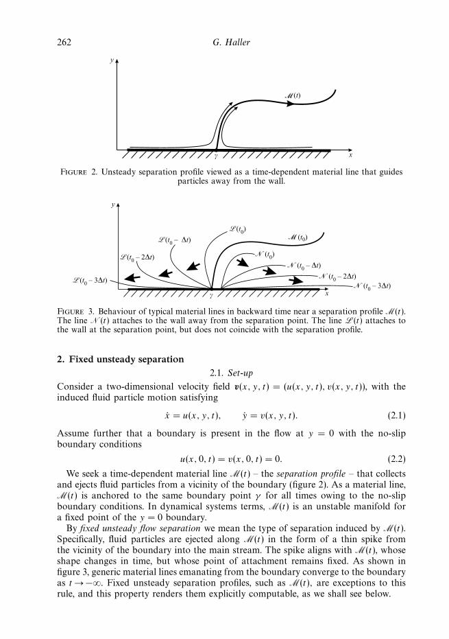
Figure 2. Unsteady separation profile viewed as a time-dependent material line that guidesparticles away from the wall.

y

x

�(t0 – 3∆t)

�(t0 – 2∆t)

� (t0 – 2∆t)� (t0 – 3∆t)

� (t0 – ∆t)

� (t0)

�(t0 – ∆t)

�(t0)� (t0)

γ

Figure 3. Behaviour of typical material lines in backward time near a separation profile M(t).The line N(t) attaches to the wall away from the separation point. The line L(t) attaches tothe wall at the separation point, but does not coincide with the separation profile.

2. Fixed unsteady separation2.1. Set-up

Consider a two-dimensional velocity field v(x, y, t) = (u(x, y, t), v(x, y, t)), with theinduced fluid particle motion satisfying

x = u(x, y, t), y = v(x, y, t). (2.1)

Assume further that a boundary is present in the flow at y = 0 with the no-slipboundary conditions

u(x, 0, t) = v(x, 0, t) = 0. (2.2)

We seek a time-dependent material line M(t) – the separation profile – that collectsand ejects fluid particles from a vicinity of the boundary (figure 2). As a material line,M(t) is anchored to the same boundary point γ for all times owing to the no-slipboundary conditions. In dynamical systems terms, M(t) is an unstable manifold fora fixed point of the y = 0 boundary.

By fixed unsteady flow separation we mean the type of separation induced by M(t).Specifically, fluid particles are ejected along M(t) in the form of a thin spike fromthe vicinity of the boundary into the main stream. The spike aligns with M(t), whoseshape changes in time, but whose point of attachment remains fixed. As shown infigure 3, generic material lines emanating from the boundary converge to the boundaryas t → −∞. Fixed unsteady separation profiles, such as M(t), are exceptions to thisrule, and this property renders them explicitly computable, as we shall see below.

Exact theory of unsteady separation 263

y

x

� (t0)

γ

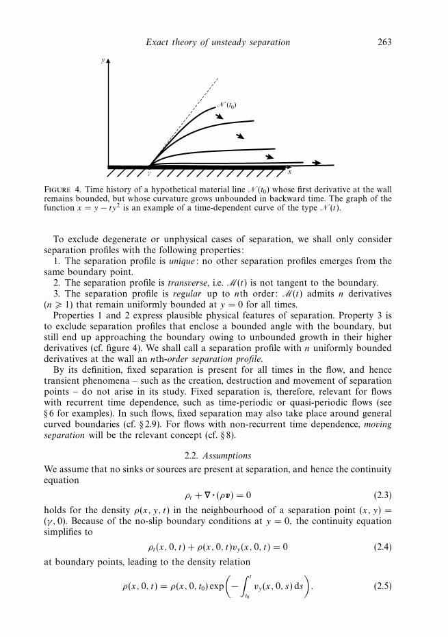
Figure 4. Time history of a hypothetical material line N(t0) whose first derivative at the wallremains bounded, but whose curvature grows unbounded in backward time. The graph of thefunction x = y − ty2 is an example of a time-dependent curve of the type N(t).

To exclude degenerate or unphysical cases of separation, we shall only considerseparation profiles with the following properties:

1. The separation profile is unique: no other separation profiles emerges from thesame boundary point.

2. The separation profile is transverse, i.e. M(t) is not tangent to the boundary.3. The separation profile is regular up to nth order: M(t) admits n derivatives

(n � 1) that remain uniformly bounded at y = 0 for all times.Properties 1 and 2 express plausible physical features of separation. Property 3 is

to exclude separation profiles that enclose a bounded angle with the boundary, butstill end up approaching the boundary owing to unbounded growth in their higherderivatives (cf. figure 4). We shall call a separation profile with n uniformly boundedderivatives at the wall an nth-order separation profile.

By its definition, fixed separation is present for all times in the flow, and hencetransient phenomena – such as the creation, destruction and movement of separationpoints – do not arise in its study. Fixed separation is, therefore, relevant for flowswith recurrent time dependence, such as time-periodic or quasi-periodic flows (see§ 6 for examples). In such flows, fixed separation may also take place around generalcurved boundaries (cf. § 2.9). For flows with non-recurrent time dependence, movingseparation will be the relevant concept (cf. § 8).

2.2. Assumptions

We assume that no sinks or sources are present at separation, and hence the continuityequation

ρt + ∇ · (ρv) = 0 (2.3)

holds for the density ρ(x, y, t) in the neighbourhood of a separation point (x, y) =(γ, 0). Because of the no-slip boundary conditions at y = 0, the continuity equationsimplifies to

ρt (x, 0, t) + ρ(x, 0, t)vy(x, 0, t) = 0 (2.4)

at boundary points, leading to the density relation

ρ(x, 0, t) = ρ(x, 0, t0) exp

(−∫ t

t0

vy(x, 0, s) ds

). (2.5)

264 G. Haller

Differentiation of (2.5) with respect to x gives the wall-tangential density gradientevolution

ρx(x, 0, t) = ρx(x, 0, t0) exp

(−∫ t

t0

vy(x, 0, s) ds

)

− ρ(x, 0, t0) exp

(−∫ t

t0

vy(x, 0, s) ds

)∫ t

t0

vxy(x, 0, s) ds. (2.6)

The density of the fluid should remain bounded from below and from above forall times along the boundary. Thus, we may assume that for appropriate ρ2 > ρ1 > 0and for all t ,

0 < ρ1 � ρ(x, 0, t) � ρ2 < ∞ (2.7)

holds along the boundary region of interest.Next we assume that the tangential density gradient along the boundary remains

uniformly bounded near the separation point for all times. In view of (2.5), (2.6) and(2.7), this second assumption is equivalent to∣∣∣∣

∫ t

t0

vxy(x, 0, s) ds

∣∣∣∣ � K1 < ∞, (2.8)

for an appropriate constant K1, for any time t , and for all x values near γ .Assumptions (2.7) and (2.8) hold automatically for incompressible flows, because

for such flows,

vy(x, 0, t) ≡ 0, vxy(x, 0, t) ≡ 0. (2.9)

2.3. Equation for the separation profile

Using the no-slip boundary condition, we rewrite (2.1) as

x = yA(x, y, t), y = yB(x, y, t), (2.10)

where

A(x, y, t) =

∫ 1

0

uy(x, sy, t) ds, B(x, y, t) =

∫ 1

0

vy(x, sy, t) ds. (2.11)

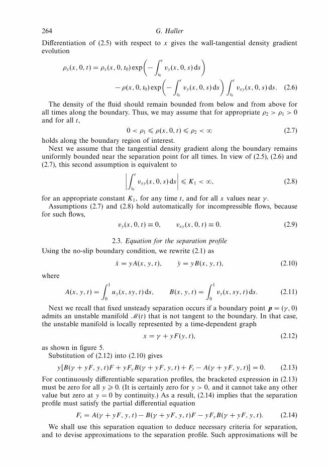
Next we recall that fixed unsteady separation occurs if a boundary point p = (γ, 0)admits an unstable manifold M(t) that is not tangent to the boundary. In that case,the unstable manifold is locally represented by a time-dependent graph

x = γ + yF (y, t), (2.12)

as shown in figure 5.Substitution of (2.12) into (2.10) gives

y[B(γ + yF, y, t)F + yFyB(γ + yF, y, t) + Ft − A(γ + yF, y, t)] = 0. (2.13)

For continuously differentiable separation profiles, the bracketed expression in (2.13)must be zero for all y � 0. (It is certainly zero for y > 0, and it cannot take any othervalue but zero at y = 0 by continuity.) As a result, (2.14) implies that the separationprofile must satisfy the partial differential equation

Ft = A(γ + yF, y, t) − B(γ + yF, y, t)F − yFyB(γ + yF, y, t). (2.14)

We shall use this separation equation to deduce necessary criteria for separation,and to devise approximations to the separation profile. Such approximations will be

Exact theory of unsteady separation 265

y

x

x = γ + yF(y, t)

γ

Figure 5. Near the wall, the separation profile can be viewed as a graph over the y variable,because we have assumed non-tangential separation.

obtained from a series expansion

F (y, t) = f0(t) + yf1(t) + 12y2f2(t) + . . . , (2.15)

where

f0(t) = F (0, t), f1(t) = Fy(0, t), f2(t) = Fyy(0, t). (2.16)

2.4. Necessary conditions for separation

To simplify our notation, we let

a(t) = A(γ, 0, t), b(t) = B(γ, 0, t), ρ(t) = ρ(γ, 0, t), (2.17)

where (γ, 0) is the separation point we wish to characterize. We also rewrite (2.5) inour new notation as

ρ(t) = ρ(t0) exp

(−∫ t

t0

b(s) ds

). (2.18)

Setting y = 0 in the separation equation (2.14), we obtain the linear differentialequation

f 0(t) = −b(t)f0(t) + a(t). (2.19)

The general solution of this equation is

f0(t) = f0(t0)ρ(t)

ρ(t0)+ ρ(t)

∫ t

t0

a(τ )

ρ(τ )dτ, (2.20)

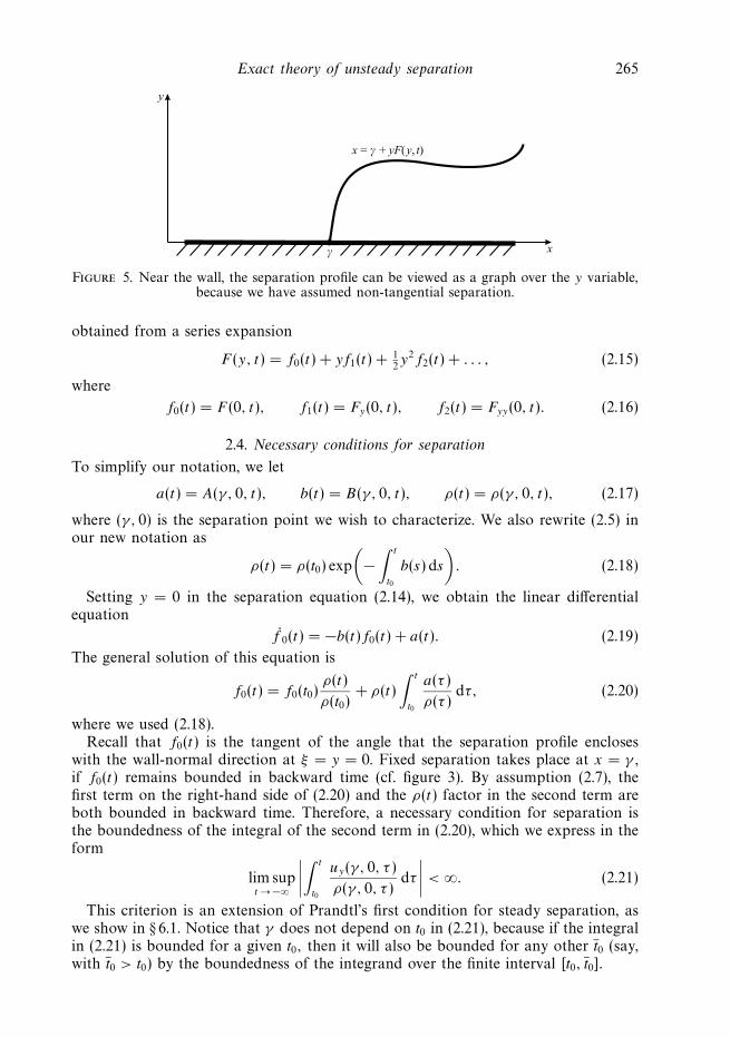
where we used (2.18).Recall that f0(t) is the tangent of the angle that the separation profile encloses

with the wall-normal direction at ξ = y = 0. Fixed separation takes place at x = γ ,if f0(t) remains bounded in backward time (cf. figure 3). By assumption (2.7), thefirst term on the right-hand side of (2.20) and the ρ(t) factor in the second term areboth bounded in backward time. Therefore, a necessary condition for separation isthe boundedness of the integral of the second term in (2.20), which we express in theform

lim supt → −∞

∣∣∣∣∫ t

t0

uy(γ, 0, τ )

ρ(γ, 0, τ )dτ

∣∣∣∣ < ∞. (2.21)

This criterion is an extension of Prandtl’s first condition for steady separation, aswe show in § 6.1. Notice that γ does not depend on t0 in (2.21), because if the integralin (2.21) is bounded for a given t0, then it will also be bounded for any other t0 (say,with t0 > t0) by the boundedness of the integrand over the finite interval [t0, t0].

266 G. Haller

Just as Prandtl’s first condition, (2.21) is also satisfied at any point of a fluid atrest, which shows the need for a second condition to describe separation. A secondnecessary condition turns out to be∫ −∞

t0

[1

ρ(τ )(uxy(γ, 0, τ ) − vyy(γ, 0, τ )) − 2vxy(γ, 0, τ )

∫ τ

t0

uy(γ, 0, s)

ρ(γ, 0, s)ds

]dτ = ∞,

(2.22)

as we show in Appendix A. This condition ensures that all material lines emanatingfrom boundary points near γ converge to the wall in backward time, a feature thatflows at rest do not possess. As we show in § 6.1, condition (2.22) simplifies to Prandtl’ssecond separation condition when applied to steady flows.

2.5. Effective separation points

The theoretical necessary condition (2.21) can be expressed in a form more suitablefor computations. To derive this equivalent form, we again recall that material linesemanating from any boundary point near (γ, 0) align with the boundary as t → −∞.By formula (2.20), this asymptotic alignment in backward time is only possible if, forall small enough |x − γ |,∫ −∞

t0

uy(x, 0, τ )

ρ(x, 0, τ )dτ =

{+ ∞ if x > γ,

− ∞ if x < γ.(2.23)

Consequently, for any large constant C > 0 and for any small δ > 0, we can selectt � t0 such that ∫ t

t0

uy(x, 0, τ )

ρ(x, 0, τ )dτ

{>C if x = γ + δ,

< −C if x = γ − δ.(2.24)

Thus, not only is the backward integral of uy/ρ bounded at separation, but it alsoadmits a sign change arbitrarily close to the separation point for large enough |t − t0|.

Because the integral

it (x) =

∫ t

t0

uy(x, 0, τ )

ρ(x, 0, τ )dτ (2.25)

is a continuous function of x for any finite t, we conclude from (2.24) that it (x) mustadmit at least one zero that approaches γ as t approaches −∞. As a result, definingthe effective separation point γeff (t, t0) via the formula∫ t

t0

uy(γeff , 0, τ )

ρ(γeff , 0, τ )dτ = 0, (2.26)

we obtain

γ = limt → −∞

γeff (t, t0), (2.27)

as shown in figure 6.Equations (2.26) and (2.27) give a practical algorithm for computing fixed unsteady

separation points at time t0 from velocity data. For a past time t with |t − t0|large enough, we compute the integral in it (x) along the wall and find the effectiveseparation point γeff (t, t0). By (2.27), this effective separation point will converge tothe real separation point γ as t → −∞.

Three remarks are in order. (i) Fixed separation points of time-periodic or time-quasi-periodic flows are exactly computable from finite-time velocity data without theuse of effective separation points (cf. § 6). (ii) The effective separation point γeff (t, t0)

Exact theory of unsteady separation 267

it (x)

γeff (t1, t0)

γeff (t2,t0)

γ x

t = t2 > t1 t = t1

Figure 6. The convergence of the effective separation point to the actual separation point.

is a good approximation for the true separation point if we select t = t0 − Tm(t0),where Tm will be defined in our discussion on moving separation (cf. § 8). (iii) Takingthe limit t → −∞ in our formulae does not require solving for the velocity field inbackward time; it requires computing longer and longer backward-time averages fromthe available velocity data as the current time t0 progresses.

2.6. Separation angle and curvature

To obtain an expression for the angle of fixed unsteady separation, we first differentiate(2.14) with respect to y and set y = 0 to obtain the equation

f 1 = axf0 + ay − bxf20 − byf0 − 2bf1. (2.28)

Our notation here is consistent with that of the previous sections; for instance, wehave ax(t) = Ax(γ, 0, t) and f1(t) = Fy(0, t).

Using the density formula (2.18), we write the solution of the above linear o.d.e. inthe form

f1(t) = f1(t0)ρ2(t)

ρ2(t0)+

∫ t

t0

ρ2(t)

ρ2(τ )

[ay(τ ) + (ax(τ ) − by(τ ))f0(τ ) − bx(τ )f 2

0 (τ )]dτ. (2.29)

For a second-order separation profile (i.e. for a profile of bounded curvature), theabove solution must be bounded as t → −∞. As we show in Appendix A, thisboundedness requirement leads to the following formula for the slope of the separationprofile at t = t0:

f0(t0) = limt → −∞

ρ(t0)

∫ t

t0

[by(τ ) − ax(τ )

ρ(τ )

∫ τ

t0

a(s)

ρ(s)ds + bx(τ )

(∫ τ

t0

a(s)

ρ(s)ds

)2

− ay(τ )

ρ2(τ )

]dτ

∫ t

t0

[ax(τ ) − by(τ )

ρ(τ )− 2bx(τ )

∫ τ

t0

a(s)

ρ(s)ds

]dτ

.

(2.30)

268 G. Haller

We recall that f0(t0) gives the separation slope measured relative to the wall-normal direction at time t = t0. Therefore, the angle of separation at (γ, 0) is α(t0) =tan−1(1/f0(t0)) when measured from the boundary.

To obtain the next coefficient in the expansion (2.15) for the separation profile, wedifferentiate (2.14) twice with respect to y and set y = 0 to obtain

f 2 = ayy + (2axy − byy)f0 + (axx − 2bxy)f20 − bxxf

30

+ 2(ax − 2by)f1 − 6bxf0 f1 − 3bf2, (2.31)

an o.d.e. for the function f2(t). The solution of this equation is

f2(t) = f2(t0)ρ3(t)

ρ3(t0)+ ρ3(t)

∫ t

t0

ayy(τ ) + f0(τ )(2axy(τ ) − byy(τ ))

ρ3(τ )dτ

+ ρ3(t)

∫ t

t0

f 20 (τ )

axx(τ ) − 2bxy(τ ) − bxx(τ )f0(τ )

ρ3(τ )dτ

+ 2ρ3(t)

∫ t

t0

f1(τ )ax(τ ) − 2by(τ ) − 3bx(τ )f0(τ )

ρ3(τ )dτ. (2.32)

Again, the right-hand side of (2.32) should be bounded for all t � t0 if ξ = yF (y, t)is the graph of a third-order separation profile. Since the first term on the right-handside is bounded by assumption (2.7), the sum of the remaining three terms must bebounded for all t � t0. Repeating the arguments leading to (11.7) and (11.11) inAppendix A, then substituting (2.29) for f (τ ) finally leads to

f1(t0) = − limt → −∞

ρ2(t0)

∫ t

t0

[R(τ ) + S(τ ) + T (τ )U (τ )] dτ∫ t

t0

ρ2(τ )T (τ ) dτ

, (2.33)

with

R(τ ) =ayy(τ ) + f0(τ )(2axy(τ ) − byy(τ ))

ρ3(τ ),

S(τ ) = f 20 (τ )

axx(τ ) − 2bxy(τ ) − bxx(τ )f0(τ )

ρ3(τ ),

T (τ ) = 2ax(τ ) − 2by(τ ) − 3bx(τ )f0(τ )

ρ3(τ ),

U (τ ) =

∫ τ

t0

ρ2(τ )

ρ2(s)

[ay(s) + (ax(s) − by(s))f0(s) − bx(s)f

20 (s)]ds.

(2.34)

Similar expressions can be derived for higher-order derivatives of F (y, t) in arecursive fashion by further differentiating the separation equation (3.8) with respectto y at y = 0. Although these expressions are lengthy for general compressible flows,they become significantly simpler for incompressible flows (see § 3).

2.7. Density-independent formulation

Using the density relation (2.5), we can express the density in terms of the integralof vy(γ, 0, t), and obtain a density-independent formulation of our fixed separation

Exact theory of unsteady separation 269

theory. In this formulation, assumptions (2.7) and (2.8) are expressed as∣∣∣∣∫ t

t0

vy(x, 0, s) ds

∣∣∣∣ � K0 < ∞,

∣∣∣∣∫ t

t0

vxy(x, 0, τ ) dτ

∣∣∣∣ � K1 < ∞, (2.35)

and the separation criteria (2.21) and (2.22) are replaced by

lim supt → −∞

∣∣∣∣∫ t

t0

exp

(∫ τ

t0

vy(γ, 0, s) ds

)uy(γ, 0, τ ) dτ

∣∣∣∣ < ∞ (2.36)

and ∫ −∞

t0

[exp

(∫ τ

t0

vy(γ, 0, s) ds

)(uxy(γ, 0, τ ) − vyy(γ, 0, τ ))

− 2vxy(γ, 0, τ )

(∫ τ

t0

exp

(∫ s

t0

vy(γ, 0, s) ds

)uy(γ, 0, s) ds

)dτ

]= ∞. (2.37)

Similarly, effective separation points are defined by the formula∫ t

t0

exp

(∫ τ

t0

vy(γeff , 0, s) ds

)uy(γeff , 0, τ ) dτ = 0. (2.38)

The separation slope and curvature, as well as higher-order derivatives of theseparation profile can all be expressed in purely kinematic terms using the densityrelation (2.5). We shall use the above density-independent formulation in derivingseparation conditions for moving boundaries in § 2.9.

2.8. Lagrangian formulation

In a series of papers, Van Dommelen and coworkers have shown that unsteadyseparation is best described in the Lagrangian frame, a point of view that we haveadopted throughout this paper. Working with Prandtl’s boundary-layer equations, VanDommelen (1981) proposes that fluid-stretching in the wall-normal direction becomesinfinitely large at the point of separation. He then uses mass conservation in theLagrangian variables to explore the implications of his postulate for the derivativesof particle positions with respect to initial states. If x(t; x0, y0, t0) denotes at time t

the x coordinate of a fluid particle that started from position (x0, y0) at time t0, VanDommelen’s criterion for boundary-layer separation at point (x, y) at time t reads

∂x(t; x0, y0, t0)

∂x0

= 0,∂x(t; x0, y0, t0)

∂y0

= 0. (2.39)

As we show in Appendix C, these conditions may only be fully satisfied for velocityfields with singularities. Another postulate implicit in (2.39) is that the separationpoint lies off the wall. By contrast, our separation criteria locate on-wall separationin general two-dimensional Navier–Stokes flows for which the velocity field is knownto remain regular.

Below we give a mathematically exact Lagrangian separation criterion forcomparison with Van Dommelen’s criteria. Our Lagrangian criterion applies to anytwo-dimensional compressible flow that remains regular along the boundary for alltimes. As we show in Appendix C, the criterion can be written as

lim supt → −∞

∣∣∣∣∂x(t; γ, 0, t0)

∂y0

∣∣∣∣ < ∞, (2.40)

where, as earlier, (γ, 0) denotes the fixed separation point on the boundary. As inthe Eulerian formulation, our Lagrangian separation criterion is approximated by the

270 G. Haller

y

y = h(x)

x

v�

(t)

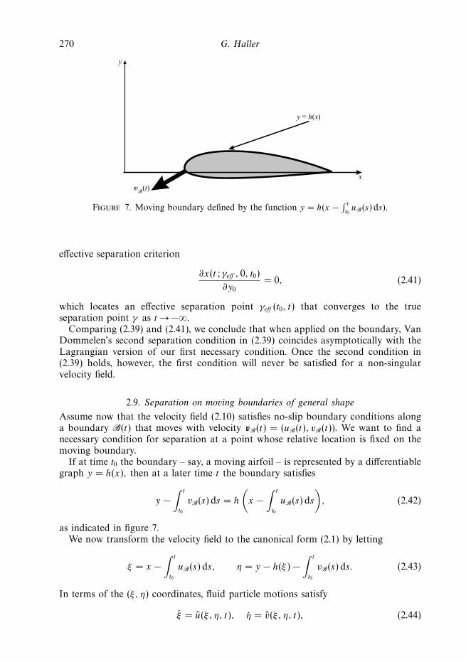
Figure 7. Moving boundary defined by the function y = h(x −∫ t

t0uB(s) ds).

effective separation criterion

∂x(t; γeff , 0, t0)

∂y0

= 0, (2.41)

which locates an effective separation point γeff (t0, t) that converges to the trueseparation point γ as t → −∞.

Comparing (2.39) and (2.41), we conclude that when applied on the boundary, VanDommelen’s second separation condition in (2.39) coincides asymptotically with theLagrangian version of our first necessary condition. Once the second condition in(2.39) holds, however, the first condition will never be satisfied for a non-singularvelocity field.

2.9. Separation on moving boundaries of general shape

Assume now that the velocity field (2.10) satisfies no-slip boundary conditions alonga boundary B(t) that moves with velocity vB(t) = (uB(t), vB(t)). We want to find anecessary condition for separation at a point whose relative location is fixed on themoving boundary.

If at time t0 the boundary – say, a moving airfoil – is represented by a differentiablegraph y = h(x), then at a later time t the boundary satisfies

y −∫ t

t0

vB(s) ds = h

(x −

∫ t

t0

uB(s) ds

), (2.42)

as indicated in figure 7.We now transform the velocity field to the canonical form (2.1) by letting

ξ = x −∫ t

t0

uB(s) ds, η = y − h(ξ ) −∫ t

t0

vB(s) ds. (2.43)

In terms of the (ξ, η) coordinates, fluid particle motions satisfy

ξ = u(ξ, η, t), η = v(ξ, η, t), (2.44)

Exact theory of unsteady separation 271

where

u(ξ, η, t) = u

(ξ +

∫ t

t0

uB(s) ds, η + h(ξ ) +

∫ t

t0

vB(s) ds, t

)− uB(t),

v(ξ, η, t) = v

(ξ +

∫ t

t0

uB(s) ds, η + h(ξ ) +

∫ t

t0

vB(s) ds, t

)− vB(t) − h′(ξ )u(ξ, η, t).

(2.45)

The transformed velocity field (u, v) satisfies the boundary conditions

u(x, 0, t) = 0, v(x, 0, t) = 0. (2.46)

Furthermore,

uξ + vη = ux + uyh′ + vy − h′uy = ux + vy, (2.47)

thus compressibility or incompressibility is unaffected by the change of coordinates(x, y) �→ (ξ, η).

Because

uη(ξ, η, t) = uy

(ξ +

∫ t

t0

uB(s) ds, η + h(ξ ) +

∫ t

t0

vB(s) ds, t

),

vη(ξ, η, t) = vy

(ξ +

∫ t

t0

uB(s) ds, η + h(ξ ) +

∫ t

t0

vB(s) ds, t

)− h′(ξ )uη(ξ, η, t),

(2.48)

the density-independent necessary condition (2.36) – applied in the (ξ, η) co-ordinates –takes the form

lim supt → −∞

∣∣∣∣∫ t

t0

E(τ, t) uy

(γ +

∫ τ

t0

uB(s) ds, h(γ ) +

∫ τ

t0

vB(r) dr, τ

)dτ

∣∣∣∣ < ∞, (2.49)

where

E(γ, τ, t) = exp

(∫ τ

t0

[vy

(γ +

∫ s

t0

uB(r) dr, h(γ ) +

∫ s

t0

vB(r) dr, s

)

− h′(γ )uy

(γ +

∫ s

t0

uB(r) dr, h(γ ) +

∫ s

t0

vB(r) dr, s

)]ds

). (2.50)

As in the case of flat boundaries, we locate the separation point on general boundariesby computing the effective separation point γeff (t, t0) for |t − t0| large enough fromthe formula∫ t

t0

E(γeff , τ, t) uy

(γeff +

∫ τ

t0

uB(s) ds, h(γeff ) +

∫ τ

t0

vB(r) dr, τ

)dτ = 0. (2.51)

To evaluate the second necessary condition (2.37) in the present (ξ, η) coordinates,we compute the second derivatives

uξη(ξ, η, t), vξη(ξ, η, t), vηη(ξ, η, t), (2.52)

in terms of the original velocity field from (2.48). With these expressions, the secondseparation condition (2.37) becomes a straightforward but lengthy condition, whichwe omit here for brevity.

272 G. Haller

γ

x

y

� (t)

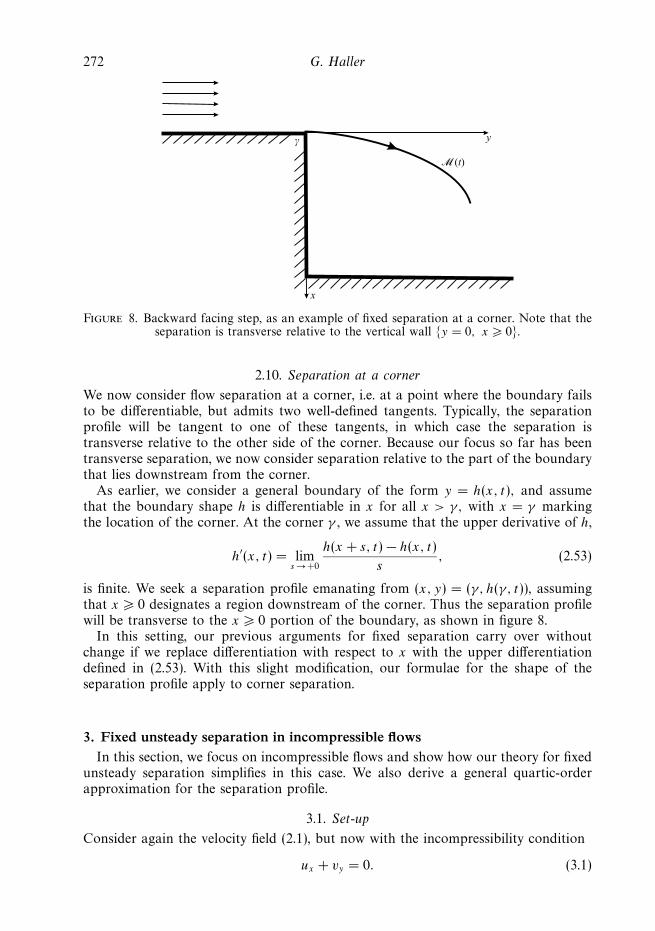
Figure 8. Backward facing step, as an example of fixed separation at a corner. Note that theseparation is transverse relative to the vertical wall {y = 0, x � 0}.

2.10. Separation at a corner

We now consider flow separation at a corner, i.e. at a point where the boundary failsto be differentiable, but admits two well-defined tangents. Typically, the separationprofile will be tangent to one of these tangents, in which case the separation istransverse relative to the other side of the corner. Because our focus so far has beentransverse separation, we now consider separation relative to the part of the boundarythat lies downstream from the corner.

As earlier, we consider a general boundary of the form y = h(x, t), and assumethat the boundary shape h is differentiable in x for all x > γ, with x = γ markingthe location of the corner. At the corner γ , we assume that the upper derivative of h,

h′(x, t) = lims → +0

h(x + s, t) − h(x, t)

s, (2.53)

is finite. We seek a separation profile emanating from (x, y) = (γ, h(γ, t)), assumingthat x � 0 designates a region downstream of the corner. Thus the separation profilewill be transverse to the x � 0 portion of the boundary, as shown in figure 8.

In this setting, our previous arguments for fixed separation carry over withoutchange if we replace differentiation with respect to x with the upper differentiationdefined in (2.53). With this slight modification, our formulae for the shape of theseparation profile apply to corner separation.

3. Fixed unsteady separation in incompressible flowsIn this section, we focus on incompressible flows and show how our theory for fixed

unsteady separation simplifies in this case. We also derive a general quartic-orderapproximation for the separation profile.

3.1. Set-up

Consider again the velocity field (2.1), but now with the incompressibility condition

ux + vy = 0. (3.1)

Exact theory of unsteady separation 273

The no-slip boundary conditions again enable us to rewrite the velocity field in theform (2.10), with the equivalent incompressibility condition

yAx + B + yBy = 0. (3.2)

Setting y = 0 in this equation gives B(x, 0, t) ≡ 0, thus we can further rewrite thevelocity field in the form

x = yA(x, y, t), y = y2C(x, y, t), (3.3)

where

C(x, y, t) =

∫ 1

0

∫ 1

0

vyy(x, spy, t)p dp ds. (3.4)

Enforcing the incompressibility condition (3.1) for system (3.3) gives the relation

y(Ax + 2C + yCy) = 0 (3.5)

between the functions A and C. Away from the boundary, i.e. for y > 0, this relationimplies

Ax + 2C + yCy = 0. (3.6)

Because Ax , C and Cy are continuous, (3.6) extends to y = 0. Therefore, (3.6) musthold all over the fluid, including the boundary.

In our arguments, we will work with the incompressible canonical velocity field(3.3) for simplicity. Alternatively, we could work with the compressible canonical form(2.10) and use the incompressibility condition (3.6), but that approach would quicklylead to intractably complex expressions.

3.2. Equation for the separation profile

As in the compressible case, we seek the unsteady separation profile in the form ofan unstable manifold satisfying ξ = x − γ = yF (y, t). Substituting this relation into(3.3) leads to the equation

y[A(yF + γ, y, t) − yC(yF + γ, y, t)(F + yFy) − Ft ] = 0. (3.7)

The bracketed expression must therefore vanish for all y � 0 by continuity, leadingto the incompressible separation equation

A(yF + γ, y, t) − yC(yF + γ, y, t)(F + yFy) − Ft = 0. (3.8)

The compressible separation equation (2.14) is equivalent to (3.8) in the case ofincompressible flows.

3.3. Necessary conditions for separation

Computing the O(1) term in the Taylor expansion of (3.8), we find that

f 0 = a, (3.9)

which implies

f0(t) = f0(t0) +

∫ t

t0

a(τ ) dτ. (3.10)

As in the compressible case, we obtain a necessary criterion at the point (γ, 0) byrequiring f0(t) to be bounded in backward time:

lim supt → −∞

∣∣∣∣∫ t

t0

uy(γ, 0, τ ) dτ

∣∣∣∣ < ∞. (3.11)

274 G. Haller

In analogy with (2.22), the further necessary condition∫ −∞

t0

uxy(γ, 0, τ ) dτ = ∞ (3.12)

must hold at fixed separation points. Note that, by incompressibility, this last conditionis equivalent to ∫ −∞

t0

vyy(γ, 0, τ ) dτ = −∞. (3.13)

3.4. Effective separation points

As noted earlier, the separation criterion (3.11) is unsuitable for direct computations.Instead, we use effective separation points defined as∫ t

t0

uy(γeff , 0, s) ds = 0, (3.14)

to approximate the location of the actual flow separation. Our argument for the con-vergence of effective separation points to actual separation points is again valid here.

3.5. Separation profile up to quartic order

We now give explicit formulae for the time-dependent coefficients of the quarticseparation profile

x = γ + f0(t)y + f1(t)y2 + 1

2f2(t)y

3 + 16f3(t)y

4. (3.15)

While these coefficients are tedious to compute for the compressible case, they becomemanageable in the present setting. As we show in Appendix B, the coefficients takethe following form when evaluated at time t0:

f0(t0) = limt → −∞

∫ t

t0

[ay(τ ) − 3c(τ )

∫ τ

t0

a(s) ds

]dτ

3

∫ t

t0

c(τ ) dτ

, (3.16)

f1(t0)

= limt → −∞

∫ t

t0

{ayy(τ ) − 8cy(τ )f0(τ ) − 4cx(τ )f 2

0 (τ ) − 8c(τ )

∫ τ

t0

[ay(s) − 3c(s)f0(s)] ds dτ

}

8

∫ t

t0

c(τ ) dτ

,

(3.17)

f2(t0) = limt → −∞

∫ t

t0

(1

15ayyy − 1

3cxxf

30 − cxyf

20 − cyyf0 − 2cyf1 − 2cx f0f1

)dτ∫ t

t0

c dτ

+

∫ t

t0

c

(∫ τ

t0

(4cxf

20 + 8cyf0 + 8cf1 − ayy

)ds

)dτ∫ t

t0

c dτ

, (3.18)

Exact theory of unsteady separation 275

f3(t0) = limt → −∞

∫ t

t0

(1

24ayyyy − 1

4cxxxxf

40 − cxxyf

30 − 3

2cxyyf

20 + cyyyf0

)dτ∫ t

t0

c dτ

− 3

∫ t

t0

(cxxf

20 f1 + 2cxyf0 f1 + cyyf1 + cx

[f 2

1 + f0f2

]+ cyf2

)dτ∫ t

t0

c dτ

+ 5

∫ t

t0

c

{∫ τ

t0

(cxxf

30 + 3cxyf

20 + 3cyyf0 + 6cxf0f1 + 6cyf1 + 3cf2 − 1

5ayyy

)ds

}dτ∫ t

t0

c dτ

.

(3.19)

4. Unsteady separation from pressure and skin frictionMonitoring and controlling unsteady separation in experiments requires separation

criteria phrased in terms of physically measurable quantities. Here we present aformulation of our separation theory in terms of pressure, skin friction, density andviscosity measured along the wall.

We recall that the skin friction τw(x, t) is defined as

τw(x, t) = νρ(x, 0, t)uy(x, 0, t), (4.1)

where ν denotes the kinematic viscosity. Using τw, we rewrite the first separationcondition (2.21) as

lim supt → −∞

∣∣∣∣∫ t

t0

τw(γ, s)

ρ2(γ, 0, s)ds

∣∣∣∣ < ∞. (4.2)

For some t < t0, the effective separation point is then computed from the equation∫ t

t0

τw(γeff (t, t0), s)

ρ2(γeff (t, t0), 0, s)ds = 0, (4.3)

thus for incompressible flows, the effective separation point coincides with the point ofzero mean-skin-friction. For compressible flows, however, the zero-mean-skin-frictionrule is generally inadequate as a true separation indicator: to obtain a good estimatefor the separation location, we need to use 1/ρ2 as a weight function when integratingthe skin friction in time.

For incompressible flows, the second separation criterion (2.22) also admits a simplekinetic formulation. Differentiating equation (4.1) with respect to x, we obtain

τ ′w(x, t) = τw(x, t)ρx(x, 0)/ρ(x, 0) + νρ(x, 0)uxy(x, 0, t), (4.4)

from which we express and substitute uxy into (2.22) to obtain the second kineticseparation criterion∫ −∞

t0

[τ ′w(x, τ )ρ(x, 0) − τw(x, τ )ρx(x, 0)] dτ = ∞. (4.5)

In addition to these necessary criteria, our separation slope formula also admitsa purely kinetic form for incompressible flows. To derive this form, we observe

276 G. Haller

that along the no-slip boundary y = 0, the incompressible Navier–Stokes equationssimplify to

px(x, 0, t)/ρ(x, 0) = νuyy(x, 0, t), vyy(x, 0, t) = −uxy(x, 0, t), (4.6)

with p(x, y, t) denoting the pressure. Combining these formulae with the definitionsof a(γ, t) and c(γ, t), we obtain the kinetic separation slope formula

f0(t0)

= limt → −∞

∫ t

t0

[νpx(γ, 0, τ )ρ2(γ, 0) + 3[τ ′

w(γ, τ )ρ(γ, 0) − τw(γ, τ )ρx(γ, 0)]

∫ τ

t0

τw(γ, τ ) ds

]dτ

3νρ(γ, 0)

∫ t

t0

[τw(γ, τ )ρx(γ, 0) − τ ′w(γ, τ )ρ(γ, 0)] dτ

.

(4.7)

If the initial density of the incompressible fluid is equal to a constant ρ0 along thewall, then the kinetic separation slope formula takes the simpler form

f0(t0) = − limt → −∞

∫ t

t0

[px(γ, 0, τ ) + 3τ ′

w(γ, τ )

∫ τ

t0

(1/νρ)τw(γ, τ ) ds

]dτ

3

∫ t

t0

τ ′w(γ, τ ) dτ

. (4.8)

Formulae (4.2) and (4.7) show that for incompressible flows, the separation locationand slope can both be monitored from pressure and skin friction sensors distributedalong the wall.

5. Sufficient conditions for sharp separationSo far we have described necessary features of fixed unsteady separation: if

separation takes place at the point (γ, 0), then conditions (2.21) and (2.22) musthold. As we argue below, a slightly stronger version of this set of conditions turns outto be sufficient: when these stronger conditions are satisfied, they guarantee the exis-tence of a time-dependent nonlinear separation profile anchored to a boundary point.

To motivate these sufficient conditions, we first note that condition (2.21) is generalenough to allow for weak separation. By weak separation we mean a scenariowhereby particles near the separation point may turn back towards the wall forfinite periods of time, and are only ejected from a vicinity of the wall asymptotically.Such weak separation behaviour is atypical in observed fluid motion where, oncestarted, separation tends to be sharp: particles in a vicinity of the separation pointmove away monotonically from the wall without turning back.

In this paper, we establish a sufficient criterion for sharp separation. To avoidlengthy technical arguments, we assume that the flow is incompressible. As we provein Appendix D, sharp incompressible separation takes place if the first necessarycondition

lim supt → −∞

∣∣∣∣∫ t

t0

uy(γ, 0, s) ds

∣∣∣∣ < ∞ (5.1)

and a stronger version of the second criterion (3.12) both hold. This stronger criterionrequires uxy to be negative and uniformly bounded away from zero for all times, i.e.

Exact theory of unsteady separation 277

requires

uxy(γ, 0, t) < −c0 < 0. (5.2)

For details of the argument, see Appendix D.As a simple Taylor expansion shows, the quantity vyy(γ, 0, t) = −uxy(γ, 0, t) is the

dominant term in the instantaneous strength of separation. Requiring it to be strictlypositive for all times ensures continued ejection of particles (sharp separation) froma vicinity of the wall. By contrast, the incompressible necessary condition (3.12) onlyrequires the asymptotic mean of vyy(γ, 0, t) to be strictly positive, and hence allowsfor weak separation.

6. Separation in flows with simple time dependenceHere, we evaluate our results for three simple classes of flows that produce

fixed separation: steady, time-periodic and quasi-periodic flows. In all three cases,separation points and profiles turn out to be exactly computable from finite-timevelocity data, and hence the use of effective separation points is unnecessary. In thesteady and time-periodic cases, we show how our criteria for the separation locationand angle agree with previous results by others. For the quasi-periodic case, no relatedresults are available in the literature.

6.1. Steady flows

6.1.1. Assumptions

For a steady compressible flow with a horizontal no-slip boundary at y = 0, thecontinuity equation (2.3) yields

ρ(x, 0)vy(x, 0) = 0. (6.1)

Because the density of the fluid is non-zero along the boundary, we obtain

vy(x, 0) = 0, (6.2)

which also implies

vxy(x, 0) = 0. (6.3)

Therefore, our main assumptions (2.7)–(2.8) are satisfied for steady flows.

6.1.2. Separation criteria

Because the density ρ(x, y) is constant in time, the first separation condition (2.21)becomes ∣∣∣∣

∫ −∞

t0

uy(γ, 0) ds

∣∣∣∣ = limt → −∞

|uy(γ, 0)(t0 − t)| < ∞. (6.4)

This condition is equivalent to

uy(γ, 0) = 0, (6.5)

which is Prandtl’s classic necessary condition for steady separation at (γ, 0) (cf. (1.1)).Differentiating the continuity equation (2.3) with respect to y, we obtain

ρ(γ, 0)[uxy(γ, 0) + vyy(γ, 0)] = 0, (6.6)

which implies

uxy(γ, 0) = −vyy(γ, 0). (6.7)

278 G. Haller

Thus, our second separation criterion (2.22) can be written as∫ −∞

t0

[uxy(γ, 0) − vyy(γ, 0)] dτ = limt → −∞

2

∫ −∞

t0

uxy(γ, 0) dτ

= limt → −∞

2uxy(γ, 0)(t − t0) = ∞, (6.8)

implyinguxy(γ, 0) < 0. (6.9)

This is Prandtl’s second condition for steady separation (cf. (1.1)).

6.1.3. Separation profile

The slope of the separation profile is given by formula (2.30), which now simplifies to

f0(t0) = limt → −∞

−∫ t

t0

ay(τ ) dτ∫ t

t0

[ax(τ ) − by(τ )] dτ

= − uyy(γ, 0)

3uxy(γ, 0), (6.10)

where we have used (6.5) and (6.7). This last equation agrees with a classic result,Lighthill’s formula for the separation slope in steady flows (Lighthill 1963). Higher-order approximations for steady separation profiles can be derived following § § 2and 3.

6.2. Time-periodic flows

6.2.1. Assumptions

If the velocity field v = (u, v) is T -periodic in time, then v and its derivatives admitFourier expansions in time. In particular, vy(x, y, t) can be written as the sum of atime-independent mean and a time-dependent oscillating part:

vy(x, y, t) = vy(x, y) + vy(x, y, t), (6.11)

where

vy(x, y) =1

T

∫ T

0

vy(x, y, t) dt,

∫ T

0

vy(x, y, t) dt = 0. (6.12)

The first major assumption in our fixed separation study was (2.7), which now takesthe particular form

lim supt → −∞

∣∣∣∣∫ t

t0

vy(x, 0, s) ds

∣∣∣∣ = lim supt → −∞

∣∣∣∣vy(x, 0) (t − t0) +

∫ t

t0

vy(x, 0, s) ds

∣∣∣∣ < ∞. (6.13)

Because vy(x, y, t) is a zero-mean periodic function of t , the integral∫ t

t0vy(x, y, s) ds

is also a zero-mean periodic function of t , and hence remains bounded for all t . Then,in view of the density formula (2.5), assumption (2.7) is equivalent to∫ T

0

vy(γ, 0, t) dt = 0. (6.14)

We stress that without this last assumption, the density at the separation pointwould tend to zero or infinity. Repeating the above argument for assumption (2.8),we obtain ∫ T

0

vxy(γ, 0, t) dt = 0, (6.15)

which prevents the unbounded growth of the wall-tangential density gradient at thepoint of separation.

Exact theory of unsteady separation 279

6.2.2. Separation criteria

Under assumption (6.14), the first separation condition (2.21) becomes

lim supt → −∞

∣∣∣∣∫ t

t0

uy(γ, 0, s)

ρ(γ, 0, s)ds

∣∣∣∣ < ∞. (6.16)

Again, the integrand in this condition is a T -periodic function, thus the integral onlyremains bounded if ∫ T

0

uy(γ, 0, t)

ρ(γ, 0, t)dt = 0, (6.17)

giving a general criterion for separation in two-dimensional time-periodic flows.For incompressible time-periodic flows, the relevant first separation criterion is

(3.11), which can only hold if ∫ T

0

uy(γ, 0, t) dt = 0. (6.18)

This agrees with the result of Shariff et al. (1991) on the location of unstablemanifolds in two-dimensional incompressible flows with a no-slip boundary. WhileYuster & Hackborn (1997) gave compressible counter-examples to the main assertionin the argument of Shariff et al., our results justify the assertion for time-periodicincompressible flows.

Our second separation criterion can also be evaluated by splitting the integrandin (2.22) into a mean and an oscillating part. This time, however, the mean must benegative for the criterion to be satisfied, thus∫ T

0

[1

ρ(t)(uxy(γ, 0, t) − vyy(γ, 0, t)) − 2vxy(γ, 0, t)

∫ t

t0

uy(γ, 0, s)

ρ(γ, 0, s)ds

]dt < 0 (6.19)

must hold for all t0. For incompressible flows, this criterion simplifies to∫ T

0

uxy(γ, 0, t) dt < 0, (6.20)

as we readily deduce from (3.12).Time-periodic flows illustrate that the lim sup operation cannot be replaced by lim

in the separation criterion (2.21). Indeed, at a fixed separation point γ , the left-handside of formula (3.11) becomes

lim supt → −∞

∣∣∣∣∫ t

t0

uy(γ, 0, τ ) dτ

∣∣∣∣ = lim supt → −∞

∣∣∣∣∫ t

t0

uy(x, y, τ ) dτ

∣∣∣∣ , (6.21)

and the integrand in this formula will have no limit as t → − ∞ for an unsteadytime-periodic velocity field.

6.2.3. Separation profile

Based on the above arguments, all our asymptotic formulae for the derivativesof the separation profile simplify to integrals over one period. For instance, theseparation angle formula (2.30) becomes

f0(t0) =

ρ(t0)

∫ T

0

[by(t) − ax(t)

ρ(t)

∫ t

t0

a(s)

ρ(s)ds + bx(t)

(∫ t

t0

a(s)

ρ(s)ds

)2

− ay(t)

ρ2(t)

]dt

∫ T

0

[ax(t) − by(t)

ρ(t)− 2bx(t)

∫ t

t0

a(s)

ρ(s)ds

]dt

. (6.22)

280 G. Haller

For incompressible flows, this formula further simplifies to

f0(t0) =

∫ T

0

[ay(t) − 3c(t)

∫ t

t0

a(s) ds

]dt

3

∫ T

0

c(t) dt

, (6.23)

as we see from (3.16). In terms of the original velocity field, condition (6.23) reads

f0(t0) =

∫ T

0

uyy(γ, 0, t) dt − 3

∫ t

t0

vyy(γ, 0, t)

∫ T

0

uy(γ, 0, s) ds dt

3

∫ T

0

vyy(γ, 0, t) dt

. (6.24)

Using the incompressibility condition vyy = −uxy , reparameterizing the domain of thedouble integral, and setting t0 = 0, we can further rewrite (6.4) as

f0(0) =

3

∫ T

0

uy(γ, 0, t)

∫ t

0

uxy(γ, 0, s) ds dt −∫ T

0

uyy(γ, 0, t) dt

3

∫ T

0

uxy(γ, 0, t) dt

, (6.25)

which agrees with formula (19) of Shariff et al. (1991). As we have mentioned above,while Yuster & Hackborn (1997) give compressible counter-examples to the generalassertion that Shariff et al. use to derive the above formula, our results show thattheir assertion is correct for incompressible time-periodic flows.

The incompressible formulae (3.17)–(3.19) simplify in the same fashion as (3.16)simplifies to (6.23): the limit of the quotient of long-term averages is replaced by thequotient of averages over one period.

6.3. Quasi-periodic flows

Quasi-periodic flows still display simple time-dependence, yet cannot be studiedthrough the repeated iteration of a single period-T map. For this reason, even partialor ad hoc separation results have been unavailable for quasi-periodic separation.Here, we show how our general separation criteria translate to simple formulae in thequasi-periodic case.

Many canonical separation problems, such as separation behind a cylinder or abackward facing step, admit a finite number of dominant frequencies in their Fourierspectrum. Such flows are approximated well by quasi-periodic velocity fields, whichare amenable to the criteria described below.

6.3.1. Assumptions

Let ω1, ω2, . . . , ωm be m numbers that are rationally independent, i.e. admit novanishing linear combination with rational coefficients. We say that the originalvelocity field (u(x, y, t), v(x, y, t)) is quasi-periodic in time with frequencies ω1, . . . , ωm,if we can write

u(x, y, t) = U (x, y, ω1t, . . . , ωmt),

v(x, y, t) = V (x, y, ω1t, . . . , ωmt),

}(6.26)

where the functions U (x, y, φ1, . . . , φm), and V (x, y, φ1, . . . , φm) are 2π-periodic ineach of the arguments φ1, . . . , φm.

Exact theory of unsteady separation 281

Quasi-periodic velocity fields can be Fourier expanded in terms of the angulararguments φi, thus we can write

u(x, y, t) = u(x, y, t) + u(x, y, t),

v(x, y, t) = v(x, y, t) + u(x, y, t),

}(6.27)

where

u(x, y, t) =1

(2π)m

∫ 2π

0

. . .

∫ 2π

0

U (x, y, φ1, . . . , φm) dφ1 . . .dφm,

v(x, y, t) =1

(2π)m

∫ 2π

0

. . .

∫ 2π

0

V (x, y, φ1, . . . , φm) dφ1 . . .dφm,

(6.28)

and (u(x, y, t), u(x, y, t)) denotes the bounded oscillatory part of the velocity. Just asin the periodic case, we perform a decomposition into mean and oscillating parts forthe quantities featured in (2.7)–(2.8), and obtain

vy(γ, 0, t) = 0, vxy(γ, 0, t) = 0, (6.29)

as the main physical assumptions for our theory. Again, these assumptions ensure theboundedness of the density and the density gradient along the wall.

6.3.2. Separation criteria

Following the arguments we gave in the periodic case, we deduce the two separationcriteria

uy(γ, 0, t)

ρ(γ, 0, t)= 0,

uxy(γ, 0, t) − vyy(γ, 0, t)

ρ(γ, 0, t)− 2vxy(γ, 0, t)

∫ t

t0

uy(γ, 0, s)

ρ(γ, 0, s)ds < 0.

(6.30)

(6.31)

Here, the second criterion must be satisfied for all t0 > 0.

6.3.3. Separation profile

Quasi-periodic separation profiles obey formulae similar to their periodiccounterparts. We simply take the periodic formulae and replace single-phase averagingover [0, T ] with multi-phase averaging as defined above. For instance, the separationslope now obeys the formula

f0(t0) = ρ(t0)

by(t) − ax(t)

ρ(t)

∫ t

t0

a(s)

ρ(s)ds + bx(t)

(∫ t

t0

a(s)

ρ(s)ds

)2

− ay(t)

ρ2(t)

ax(t) − by(t)

ρ(t)− 2bx(t)

∫ t

t0

a(s)

ρ(s)ds

, (6.32)

simplifying to

f0(t0) =

ay(t) − 3c(t)

∫ t

t0

a(s) ds

3c(t)(6.33)

in the incompressible case. We omit the remaining higher-order expressions for brevity.

282 G. Haller

y

xγ

� (t)

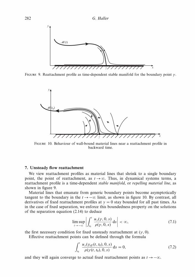
Figure 9. Reattachment profile as time-dependent stable manifold for the boundary point γ .

y

xγ

� (t0)

Figure 10. Behaviour of wall-bound material lines near a reattachment profile inbackward time.

7. Unsteady flow reattachmentWe view reattachment profiles as material lines that shrink to a single boundary

point, the point of reattachment, as t → ∞. Thus, in dynamical systems terms, areattachment profile is a time-dependent stable manifold, or repelling material line, asshown in figure 9.

Material lines that emanate from generic boundary points become asymptoticallytangent to the boundary in the t → −∞ limit, as shown in figure 10. By contrast, allderivatives of fixed reattachment profiles at y = 0 stay bounded for all past times. Asin the case of fixed separation, we enforce this boundedness property on the solutionsof the separation equation (2.14) to deduce

lim supt → −∞

∣∣∣∣∫ t

t0

uy(γ, 0, s)

ρ(γ, 0, s)ds

∣∣∣∣ < ∞, (7.1)

the first necessary condition for fixed unsteady reattachment at (γ, 0).Effective reattachment points can be defined through the formula∫ t

t0

uy(γeff (t, t0), 0, s)

ρ(γ (t, t0), 0, s)ds = 0, (7.2)

and they will again converge to actual fixed reattachment points as t → −∞.

Exact theory of unsteady separation 283

y

x

γ (t)

� (t)

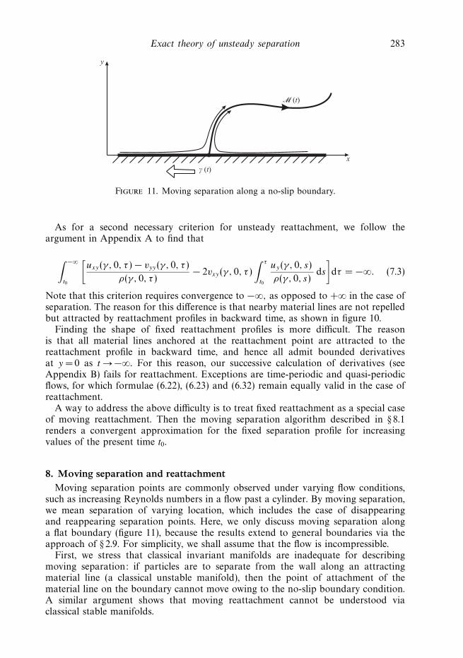
Figure 11. Moving separation along a no-slip boundary.

As for a second necessary criterion for unsteady reattachment, we follow theargument in Appendix A to find that

∫ −∞

t0

[uxy(γ, 0, τ ) − vyy(γ, 0, τ )

ρ(γ, 0, τ )− 2vxy(γ, 0, τ )

∫ τ

t0

uy(γ, 0, s)

ρ(γ, 0, s)ds

]dτ = −∞. (7.3)

Note that this criterion requires convergence to −∞, as opposed to +∞ in the case ofseparation. The reason for this difference is that nearby material lines are not repelledbut attracted by reattachment profiles in backward time, as shown in figure 10.

Finding the shape of fixed reattachment profiles is more difficult. The reasonis that all material lines anchored at the reattachment point are attracted to thereattachment profile in backward time, and hence all admit bounded derivativesat y = 0 as t → −∞. For this reason, our successive calculation of derivatives (seeAppendix B) fails for reattachment. Exceptions are time-periodic and quasi-periodicflows, for which formulae (6.22), (6.23) and (6.32) remain equally valid in the case ofreattachment.

A way to address the above difficulty is to treat fixed reattachment as a special caseof moving reattachment. Then the moving separation algorithm described in § 8.1renders a convergent approximation for the fixed separation profile for increasingvalues of the present time t0.

8. Moving separation and reattachmentMoving separation points are commonly observed under varying flow conditions,

such as increasing Reynolds numbers in a flow past a cylinder. By moving separation,we mean separation of varying location, which includes the case of disappearingand reappearing separation points. Here, we only discuss moving separation alonga flat boundary (figure 11), because the results extend to general boundaries via theapproach of § 2.9. For simplicity, we shall assume that the flow is incompressible.

First, we stress that classical invariant manifolds are inadequate for describingmoving separation: if particles are to separate from the wall along an attractingmaterial line (a classical unstable manifold), then the point of attachment of thematerial line on the boundary cannot move owing to the no-slip boundary condition.A similar argument shows that moving reattachment cannot be understood viaclassical stable manifolds.

284 G. Haller

The key to understanding moving separation is a recent development in dynamicalsystems, the concept of finite-time invariant manifolds (Haller & Poje 1998; Haller2000, 2001). A finite-time unstable manifold is a material curve that acts as anunstable manifold for a fixed point only over a finite time interval I. In morephysical terms, a finite-time unstable manifold is a material line that attracts allnearby fluid particles over I.

When a finite-time unstable manifold ceases to attract, another nearby material linemay become attracting. Then the second material line will act as a separation profilefor a while, attracting all nearby material lines, including the one that used to be theseparation profile. Later, the second material line may also lose its attracting property,and give its place to a nearby third material line that has just become attracting.

If the above process repeats itself, we observe a sliding separation point createdby attachment points of different material lines, each of which acts as a finite-timeseparation profile. Similarly, moving reattachment can be thought of as the sliding offinite-time attracting material lines along a no-slip wall.

8.1. Heuristic necessary condition

Here we give a numerically assisted necessary condition for moving separation inincompressible flows. This criterion assumes that the backward-time integral of theskin friction has a well-defined mean component that can be extracted numericallyor analytically. The criterion is heuristic in that it does not address the existence of afinite-time invariant manifold; it simply assumes the presence of a moving point atwhich the fluid breaks away from the boundary.

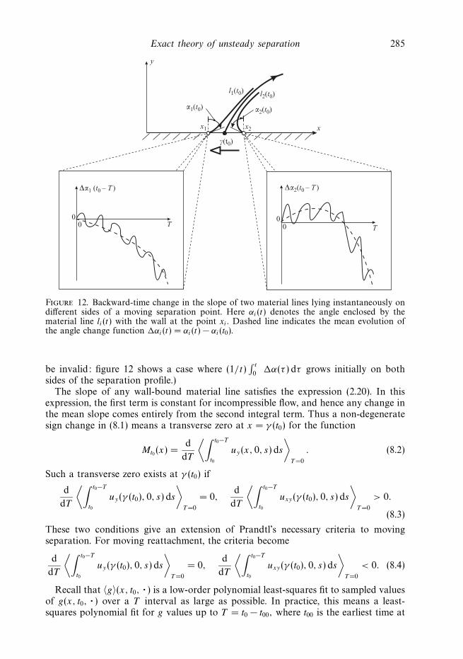
Consider a moving separation point that lies at x = γ (t0) at time t0. For concreteness,assume that the instantaneous velocity of the separation profile is negative, as shownin figure 12. Let l1(t) be a material line based at a boundary point x1 that is onthe left-hand side of the moving separation profile at time t0. The motion of l1(t) istypically aperiodic, but for the separation to be observable in the Lagrangian frame,the mean component of the slope of l1(t) must grow; we assume that this is the case.

In our arguments below, the mean component of a function f (t) (denoted 〈f 〉(t))will be a low-order polynomial least-squares fit to sampled values of f (t). The sampledvalues are taken from the interval [0, T ], where T and the number of samples areas large as possible. In analytic examples, the mean component may be exactlyidentifiable without a numerical least-squares fit (for example, 〈t + sin t〉 = t).

Because the separation profile repels l1(t) in backward time, the mean componentof the slope of l1(t) relative to the vertical will decrease for decreasing t < t0 values,as shown schematically in figure 12. By contrast, the mean slope of a material linel2(t) anchored at the point x2 on the right-hand side of the profile will initially growin backward time. This trend changes once the backward-moving profile passes x2:the mean component of the slope of l2(t) will then decrease for further decreasingvalues of t (see figure 12).

As a consequence, the derivative

d

dT[〈�α〉(x, t0 − T )]T =0 (8.1)

of the mean-angle-change function 〈�α〉(x, t0 − T ) changes sign from negative topositive at the moving separation point x = γ (t0). Thus, in the case of non-degeneratemoving separation, (d/dT )[〈�α〉(x, t0 −T )]T =0 has a transverse zero at x = γ (t0). (With

the customary mean definition 〈�α〉 = (1/t)∫ t

0�α(τ ) dτ , this last conclusion would

Exact theory of unsteady separation 285

y

x

α1(t0) α2(t0)

∆α2(t0 – T )∆α1 (t0 – T )

l1(t0) l2(t0)

x1 x2

γ(t0)

00 0

0TT

Figure 12. Backward-time change in the slope of two material lines lying instantaneously ondifferent sides of a moving separation point. Here αi(t) denotes the angle enclosed by thematerial line li(t) with the wall at the point xi . Dashed line indicates the mean evolution ofthe angle change function �αi(t) = αi(t) − αi(t0).

be invalid: figure 12 shows a case where (1/t)∫ t

0�α(τ ) dτ grows initially on both

sides of the separation profile.)The slope of any wall-bound material line satisfies the expression (2.20). In this

expression, the first term is constant for incompressible flow, and hence any change inthe mean slope comes entirely from the second integral term. Thus a non-degeneratesign change in (8.1) means a transverse zero at x = γ (t0) for the function

Mt0 (x) =d

dT

⟨∫ t0−T

t0

uy(x, 0, s) ds

⟩T =0

. (8.2)

Such a transverse zero exists at γ (t0) if

d

dT

⟨∫ t0−T

t0

uy(γ (t0), 0, s) ds

⟩T =0

= 0,d

dT

⟨∫ t0−T

t0

uxy(γ (t0), 0, s) ds

⟩T =0

> 0.

(8.3)

These two conditions give an extension of Prandtl’s necessary criteria to movingseparation. For moving reattachment, the criteria become

d

dT

⟨∫ t0−T

t0

uy(γ (t0), 0, s) ds

⟩T =0

= 0,d

dT

⟨∫ t0−T

t0

uxy(γ (t0), 0, s) ds

⟩T =0

< 0. (8.4)

Recall that 〈g〉(x, t0, · ) is a low-order polynomial least-squares fit to sampled valuesof g(x, t0, · ) over a T interval as large as possible. In practice, this means a least-squares polynomial fit for g values up to T = t0 − t00, where t00 is the earliest time at

286 G. Haller

which velocity data is available. For a faithful approximation of 〈g〉, the order of theleast-squares polynomial should be low relative to the number of sampled values forg. In our later numerical experiments, the order three or four was selected.

With increasing T , 〈g〉 gives an increasingly accurate representation of the meanevolution of

∫uy ds. As a result, transverse zeros of Mt0 (x) converge to moving

separation or reattachment points as the present time t0 becomes sufficiently far fromt00.

The derivatives of a moving separation profile at the wall can be determinedby repeating the argument leading to (8.2). For instance, the mean curvature of l1(t)decreases in backward time for t < t0, while the mean curvature of l2(t) only decreasesin backward time after an initial period of increase. Assuming incompressibility, weuse the curvature formula (12.6) to find that

Nt0 (x) =d

dT

⟨∫ t0−T

t0

[uyy(x, 0, τ ) − 3vyy(x, 0, τ )

(f0(t0) +

∫ τ

t0

uy(x, 0, s) ds

)]dτ

⟩T =0

(8.5)

has a transverse zero at x = γ (t0), with f0(t0) denoting the slope of the separationprofile at t = t0. As a result, we obtain

f0(t0) =

(d/dT )

⟨∫ t0−T

t0

[uyy(γ (t0), 0, τ ) − 3vyy(γ (t0), 0, τ )

∫ τ

t0

uy(γ (t0), 0, s) ds

]dτ

⟩T =0

3(d/dT )

⟨∫ t0−T

t0

vyy(γ (t0), 0, τ ) dτ

⟩T =0

.

(8.6)

Higher derivatives of the moving separation profile are obtained in a similar fashion.As opposed to the case of fixed separation profiles, (8.6) is equally valid for moving

flow reattachment. This is because (8.6) follows from a bifurcation in short-termmaterial line behaviour that is also present in moving reattachment.

We recall that moving separation profiles are inherently non-unique. The formulaegiven above single out the separation profile that attracts nearby material lines atthe highest rate. The numerical extraction of the mean component 〈g〉 is also a non-unique procedure, but it is the bifurcation of 〈g〉 that defines the moving separationlocation, not the actual values of 〈g〉. In our numerical experiments (see § 9) we foundthe separation location to be robust with respect to changes in the order of thepolynomial least-squares fit producing 〈g〉.

8.2. Analytic sufficient condition

Moving separation can also be treated in rigorous analytic terms without assuminga well-defined mean for the skin friction integral. First, for the present time t0, wecompute the effective separation point γeff (t, t0) for all available t < t0, then identifythe upper and lower bounds

γ+(t, t0) = sups∈[t,t0)

γeff (s, t0), γ−(t, t0) = infs∈[t,t0)

γeff (s, t0), (8.7)

on γeff (t, t0). Let the maximal x distance travelled by γeff (s, t0) over the interval [t, t0)be denoted by

δ(t, t0) = γ+(t, t0) − γ−(t, t0), (8.8)

Exact theory of unsteady separation 287

which is the length of the interval

I (t, t0) = [γ−(t, t0), γ+(t, t0)]. (8.9)

Finally, assume that the flow is incompressible.In Appendix E, we prove the existence of finite-time sharp separation at the point

γ (t0) = 12[γ+(t0 − Tm(t0), t0) + γ−(t0 − Tm(t0), t0)], (8.10)

where Tm(t0) is the smallest time for which

12δ(t0 − Tm(t0), t0)

∫ t0

t0−Tm(t0)

maxx∈I (t0−Tm(t0),t0)

|uxy(x, 0, t)| dt = 1, (8.11)

maxx∈I (t0−Tm(t0),t0)

uxy(x, 0, t) < 0, t ∈ [t0 − Tm(t0), t0]. (8.12)

The above conditions distinguish one finite-time unstable manifold out of theinfinitely many near the moving separation point. For specific velocity fields, theconditions may be further sharpened (see Appendix E). A similar result holds formoving reattachment points, except that the second condition in (8.11) is replaced by

maxx∈I (t0−Tm(t0),t0)

uxy(x, 0, t) > 0, t ∈ [t0 − Tm(t0), t0]. (8.13)

To obtain derivatives of the moving separation profile at time t0, we use the timescale Tm(t0) to evaluate our earlier derivative formulae for fixed separation. Forinstance, if the flow is incompressible, we use the finite-time version of (3.16) todeduce the moving separation slope formula

f0(t0) =

∫ t0−Tm(t0)

t0

[ay(τ ) − 3c(τ )

∫ τ

t0

a(s) ds

]dτ

3

∫ t−Tm(t0)

t0

c(τ ) dτ

. (8.14)

Again, recall that moving separation profiles are non-unique. For any present timet0, the above criterion singles out the profile that has remained close to an effectiveseparation point γeff (t, t0) for the longest time.

9. An example: unsteady separation bubble at a no-slip wallIn this section, we test our unsteady separation and reattachment formulae on

variants of an unsteady separation bubble flow derived by Ghosh et al. (1998). Ghoshet al. use the algorithm of Perry & Chong (1986) to derive a low-order approximationto separation bubble solutions of the Navier–Stokes equations. Simple but dynamicallyrelevant, this flow model allows a detailed comparison between our theory and actualflow separation displayed by fluid particles. Numerically more challenging flows willbe treated elsewhere.

9.1. Time-periodic separation bubble

We first consider the original velocity field derived by Ghosh et al. (1998) for thestudy of passive scalar transport near an unsteady separation bubble. The velocityfield is of the form

u(x, y, t) = −y + 3y2 + x2y − 23y3 + βxy sinωt,

v(x, y, t) = −xy2 − 12βy2 sinωt,

}(9.1)

288 G. Haller

with the wall located at y = 0. Because the flow is incompressible, our mainassumptions (6.14) and (6.15) for time-periodic flows are satisfied.

Evaluating conditions (6.18) and (6.20), we obtain

∫ T

0

uy(γ, 0, t) dt =

∫ T

0

(−1 + γ 2 + βγ sinωt) dt = (γ 2 − 1)2π

ω,

∫ T

0

vyy(γ, 0, t) dt =

∫ T

0

(−2γ − β sinωt) dt = −2γ2π

ω,

(9.2)

and hence fixed separation points must satisfy |γ | = 1 and γ < 0, and fixedreattachment points must satisfy |γ | = 1 and γ > 0. Separation and reattachmentpoints must therefore lie at

γ = − 1, γ = +1, (9.3)

respectively, in agreement with the numerical observation of Ghosh et al.At time t , the derivatives of the separation profile emanating from (x, y) = (−1, 0)

obey (3.16)–(3.19). Because the velocity field is time-periodic, (3.16)–(3.19) simplify toquotients of averages over one period, as we remarked at the end of § 6.2. Computingthese averages, we find that

f0(t) = 1 +β

ωcos ωt,

f1(t) =1

3− β2

2ω2− 3β

2ωcos ωt − 4β

ω2sinωt − 3β2

8ω2cos 2ωt,

f2(t) =2

3+

5β2

2ω2+

β

ω

(5

4

β2

ω2− 24

ω2− 4

3

)cosωt +

20β

ω2sinωt

+3β2

2ω2cos 2ωt +

11β2

2ω3sin 2ωt +

β3

4ω3cos 3ωt,

f3(t) =7

3+

33

8

β2

ω2− 237

128

β4

ω4+

135

2

β2

ω4+

β

ω2

(360

ω2− 75

4

β2

ω2− 15

)sinωt

+β

ω

(390

ω2− 105

8

β2

ω2− 5

)cosωt +

β2

ω2

(5

2− 15

8

β2

ω2+

435

4ω2

)cos 2ωt

− 525

8

β2

ω3sin 2ωt − β3

ω3

(15

8+

10

ω

)sin 3ωt − 15

64

β4

ω4cos 4ωt.

(9.4)

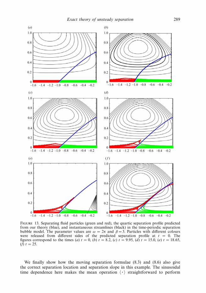
Using these expressions, we have computed the unsteady separation profile up toquartic order and compared it with the actual time evolution of the fluid near theboundary. Advecting a thin layer of fluid particles in time, we have found that theyindeed separate from the wall along the time-dependent separation profile predictedby our theory (figure 13). For comparison, we also show instantaneous streamlinesin the figure, noting that the instantaneous streamline separation point (zero skinfriction point) has no direct relationship to the true separation point. Also note thatjust as in the steady case (figure 1), flow separation starts with the formation of a tipaway from the actual point of separation, with the true separation point and profileonly prevailing later.

Exact theory of unsteady separation 289

1.0

0.8

0.6

0.4

0.2

–1.6 –1.4 –1.2 –1.0 –0.8 –0.6 –0.4 –0.2 –1.6 –1.4 –1.2 –1.0 –0.8 –0.6 –0.4 –0.2

–1.6 –1.4 –1.2 –1.0 –0.8 –0.6 –0.4 –0.2

–1.6 –1.4 –1.2 –1.0 –0.8 –0.6 –0.4 –0.2

–1.6 –1.4 –1.2 –1.0 –0.8 –0.6 –0.4 –0.2

–1.6 –1.4 –1.2 –1.0 –0.8 –0.6 –0.4 –0.2

0

1.0

0.8

0.6

0.4

0.2

0

1.0

0.8

0.6

0.4

0.2

0

1.0

0.8

0.6

0.4

0.2

0

1.0

0.8

0.6

0.4

0.2

0

1.0

0.8

0.6

0.4

0.2

0

(c)

(e) ( f )

(d)

(b)(a)

Figure 13. Separating fluid particles (green and red), the quartic separation profile predictedfrom our theory (blue), and instantaneous streamlines (black) in the time-periodic separationbubble model. The parameter values are ω = 2π and β = 3. Particles with different colourswere released from different sides of the predicted separation profile at t = 0. Thefigures correspond to the times (a) t = 0, (b) t = 8.2, (c) t = 9.95, (d) t = 15.0, (e) t = 18.65,(f) t = 25.

We finally show how the moving separation formulae (8.3) and (8.6) also givethe correct separation location and separation slope in this example. The sinusoidaltime dependence here makes the mean operation 〈 · 〉 straightforward to perform

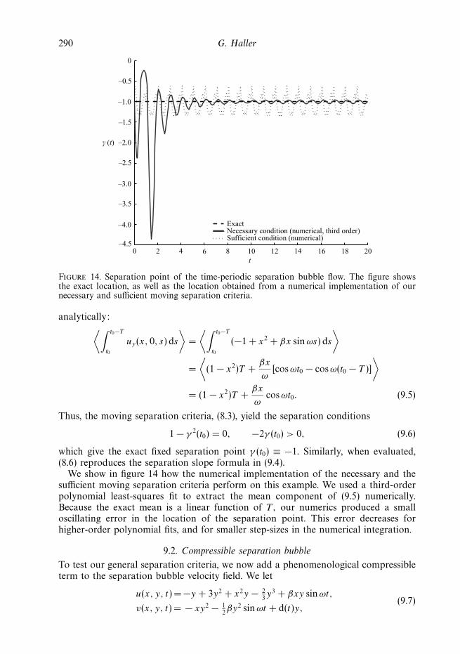
290 G. Haller

0 2 4 6 8 10 12 14 16 18 20–4.5

–4.0

–3.5

–3.0

–2.5

–2.0

–1.5

–1.0

–0.5

0

ExactNecessary condition (numerical, third order)Sufficient condition (numerical)

t

γ (t)

Figure 14. Separation point of the time-periodic separation bubble flow. The figure showsthe exact location, as well as the location obtained from a numerical implementation of ournecessary and sufficient moving separation criteria.

analytically:⟨∫ t0−T

t0

uy(x, 0, s) ds

⟩=

⟨∫ t0−T

t0

(−1 + x2 + βx sinωs) ds

⟩

=

⟨(1 − x2)T +

βx

ω[cos ωt0 − cosω(t0 − T )]

⟩

= (1 − x2)T +βx

ωcosωt0. (9.5)

Thus, the moving separation criteria, (8.3), yield the separation conditions

1 − γ 2(t0) = 0, −2γ (t0) > 0, (9.6)

which give the exact fixed separation point γ (t0) ≡ −1. Similarly, when evaluated,(8.6) reproduces the separation slope formula in (9.4).

We show in figure 14 how the numerical implementation of the necessary and thesufficient moving separation criteria perform on this example. We used a third-orderpolynomial least-squares fit to extract the mean component of (9.5) numerically.Because the exact mean is a linear function of T , our numerics produced a smalloscillating error in the location of the separation point. This error decreases forhigher-order polynomial fits, and for smaller step-sizes in the numerical integration.

9.2. Compressible separation bubble

To test our general separation criteria, we now add a phenomenological compressibleterm to the separation bubble velocity field. We let

u(x, y, t) = −y + 3y2 + x2y − 23y3 + βxy sinωt,

v(x, y, t) = − xy2 − 12βy2 sinωt + d(t)y,

(9.7)

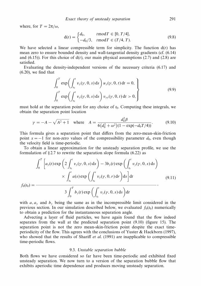
Exact theory of unsteady separation 291

where, for T = 2π/ω,

d(t) =

{d0, tmodT ∈ [0, T /4],

−d0/3, tmodT ∈ (T/4, T ).(9.8)

We have selected a linear compressible term for simplicity. The function d(t) hasmean zero to ensure bounded density and wall-tangential density gradients (cf. (6.14)and (6.15)). For this choice of d(t), our main physical assumptions (2.7) and (2.8) aresatisfied.

Evaluating the density-independent versions of the necessary criteria (6.17) and(6.20), we find that∫ T

0

exp

(∫ t

t0

vy(γ, 0, s) ds

)uy(γ, 0, t) dt = 0,

∫ T

0

exp

(∫ t

t0

vy(γ, 0, s) ds

)vyy(γ, 0, t) dt > 0,

(9.9)

must hold at the separation point for any choice of t0. Computing these integrals, weobtain the separation point location

γ = −A −√

A2 + 1 where A =d2

0β

6(d2

0 + ω2)(1 − exp(−d0T/4))

. (9.10)

This formula gives a separation point that differs from the zero-mean-skin-frictionpoint x = −1 for non-zero values of the compressibility parameter d0, even thoughthe velocity field is time-periodic.

To obtain a linear approximation for the unsteady separation profile, we use theformulation of § 2.7 to rewrite the separation slope formula (6.22) as

f0(t0) =

∫ T

0

[ay(t) exp

(2

∫ t

t0

vy(γ, 0, s) ds

)− 3by(t) exp

(∫ t

t0

vy(γ, 0, s) ds

)

×∫ t

t0

a(s) exp

(∫ s

t0

vy(γ, 0, r) dr

)ds

]dt

,

3

∫ T

0

by(t) exp

(∫ t

t0

vy(γ, 0, s) ds

)dt

(9.11)

with a, ay and by being the same as in the incompressible limit considered in theprevious section. In our simulation described below, we evaluated f0(t0) numericallyto obtain a prediction for the instantaneous separation angle.

Advecting a layer of fluid particles, we have again found that the flow indeedseparates from the wall at the predicted separation point (9.10) (figure 15). Theseparation point is not the zero mean-skin-friction point despite the exact time-periodicity of the flow. This agrees with the conclusions of Yuster & Hackborn (1997),who showed that the results of Shariff et al. (1991) are inapplicable to compressibletime-periodic flows.

9.3. Unstable separation bubble

Both flows we have considered so far have been time-periodic and exhibited fixedunsteady separation. We now turn to a version of the separation bubble flow thatexhibits aperiodic time dependence and produces moving unsteady separation.

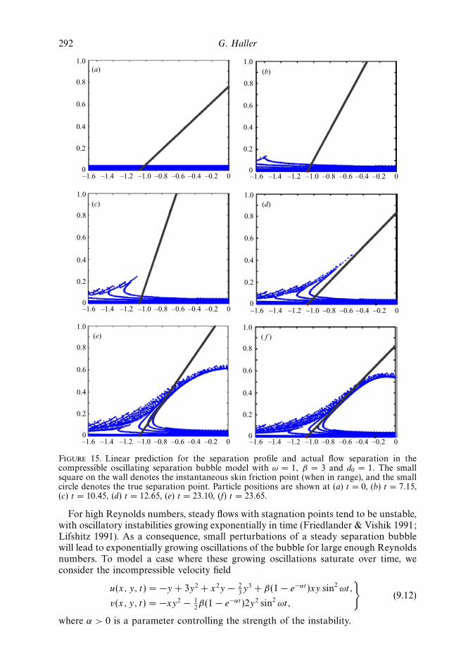
292 G. Haller

1.0

0.8

0.6

0.4

0.2

0

1.0

0.8

0.6

0.4

0.2

0

1.0

0.8

0.6

0.4

0.2

0

1.0

0.8

0.6

0.4

0.2

0

1.0

0.8

0.6

0.4

0.2

0

1.0

0.8

0.6

0.4

0.2

0

–1.6 –1.4 –1.2 –1.0 –0.8 –0.6 –0.4 –0.2 0 –1.6 –1.4 –1.2 –1.0 –0.8 –0.6 –0.4 –0.2 0

–1.6 –1.4 –1.2 –1.0 –0.8 –0.6 –0.4 –0.2 0

–1.6 –1.4 –1.2 –1.0 –0.8 –0.6 –0.4 –0.2 0

–1.6 –1.4 –1.2 –1.0 –0.8 –0.6 –0.4 –0.2 0

–1.6 –1.4 –1.2 –1.0 –0.8 –0.6 –0.4 –0.2 0

(a) (b)

(c) (d)

(e) ( f )

Figure 15. Linear prediction for the separation profile and actual flow separation in thecompressible oscillating separation bubble model with ω = 1, β = 3 and d0 = 1. The smallsquare on the wall denotes the instantaneous skin friction point (when in range), and the smallcircle denotes the true separation point. Particle positions are shown at (a) t = 0, (b) t = 7.15,(c) t = 10.45, (d) t = 12.65, (e) t = 23.10, (f) t = 23.65.

For high Reynolds numbers, steady flows with stagnation points tend to be unstable,with oscillatory instabilities growing exponentially in time (Friedlander & Vishik 1991;Lifshitz 1991). As a consequence, small perturbations of a steady separation bubblewill lead to exponentially growing oscillations of the bubble for large enough Reynoldsnumbers. To model a case where these growing oscillations saturate over time, weconsider the incompressible velocity field

u(x, y, t) = −y + 3y2 + x2y − 23y3 + β(1 − e−αt )xy sin2 ωt,

v(x, y, t) = −xy2 − 12β(1 − e−αt )2y2 sin2 ωt,

}(9.12)

where α > 0 is a parameter controlling the strength of the instability.

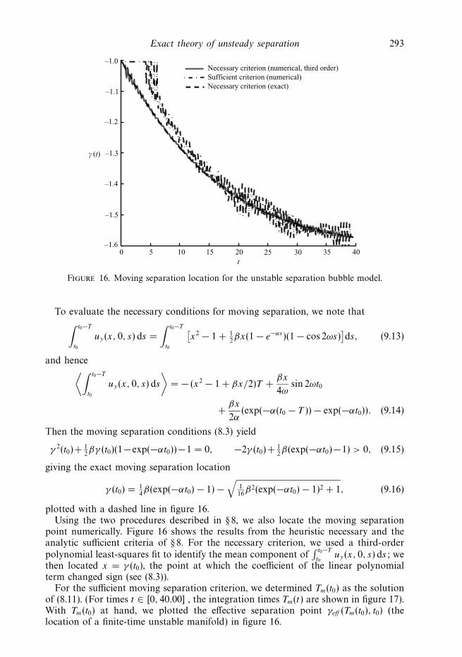
Exact theory of unsteady separation 293

0 5 10 15 20 25 30 35 40–1.6

–1.5

–1.4

–1.3

–1.2

–1.1

–1.0Necessary criterion (numerical, third order)Sufficient criterion (numerical)Necessary criterion (exact)

t

γ (t)

Figure 16. Moving separation location for the unstable separation bubble model.

To evaluate the necessary conditions for moving separation, we note that∫ t0−T

t0

uy(x, 0, s) ds =

∫ t0−T

t0

[x2 − 1 + 1

2βx(1 − e−αs)(1 − cos 2ωs)

]ds, (9.13)

and hence⟨∫ t0−T

t0

uy(x, 0, s) ds

⟩= − (x2 − 1 + βx/2)T +

βx

4ωsin 2ωt0

+βx

2α(exp(−α(t0 − T )) − exp(−αt0)). (9.14)

Then the moving separation conditions (8.3) yield

γ 2(t0)+12βγ (t0)(1−exp(−αt0))−1 = 0, −2γ (t0)+

12β(exp(−αt0)−1) > 0, (9.15)

giving the exact moving separation location

γ (t0) = 14β(exp(−αt0) − 1) −

√116

β2(exp(−αt0) − 1)2 + 1, (9.16)

plotted with a dashed line in figure 16.Using the two procedures described in § 8, we also locate the moving separation

point numerically. Figure 16 shows the results from the heuristic necessary and theanalytic sufficient criteria of § 8. For the necessary criterion, we used a third-orderpolynomial least-squares fit to identify the mean component of

∫ t0−T

t0uy(x, 0, s) ds; we

then located x = γ (t0), the point at which the coefficient of the linear polynomialterm changed sign (see (8.3)).

For the sufficient moving separation criterion, we determined Tm(t0) as the solutionof (8.11). (For times t ∈ [0, 40.00] , the integration times Tm(t) are shown in figure 17).With Tm(t0) at hand, we plotted the effective separation point γeff (Tm(t0), t0) (thelocation of a finite-time unstable manifold) in figure 16.

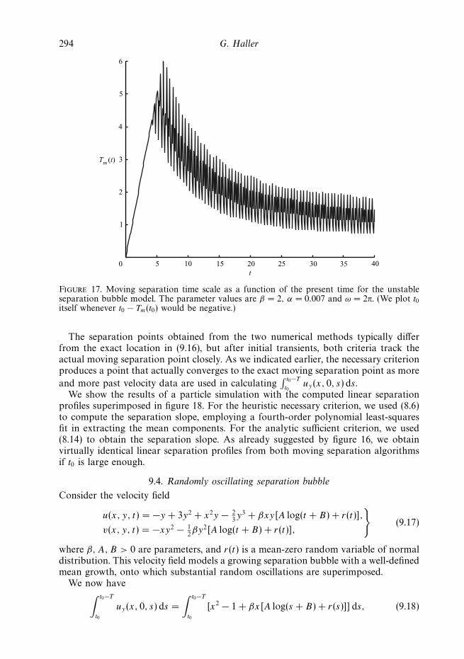
294 G. Haller

5 10 15 20 25 30 35 400

1

2

3

4

5

6

t

Tm (t)

Figure 17. Moving separation time scale as a function of the present time for the unstableseparation bubble model. The parameter values are β = 2, α = 0.007 and ω = 2π. (We plot t0itself whenever t0 − Tm(t0) would be negative.)

The separation points obtained from the two numerical methods typically differfrom the exact location in (9.16), but after initial transients, both criteria track theactual moving separation point closely. As we indicated earlier, the necessary criterionproduces a point that actually converges to the exact moving separation point as more

and more past velocity data are used in calculating∫ t0−T

t0uy(x, 0, s) ds.

We show the results of a particle simulation with the computed linear separationprofiles superimposed in figure 18. For the heuristic necessary criterion, we used (8.6)to compute the separation slope, employing a fourth-order polynomial least-squaresfit in extracting the mean components. For the analytic sufficient criterion, we used(8.14) to obtain the separation slope. As already suggested by figure 16, we obtainvirtually identical linear separation profiles from both moving separation algorithmsif t0 is large enough.

9.4. Randomly oscillating separation bubble

Consider the velocity field

u(x, y, t) = −y + 3y2 + x2y − 23y3 + βxy[A log(t + B) + r(t)],

v(x, y, t) = −xy2 − 12βy2[A log(t + B) + r(t)],

}(9.17)

where β, A, B > 0 are parameters, and r(t) is a mean-zero random variable of normaldistribution. This velocity field models a growing separation bubble with a well-definedmean growth, onto which substantial random oscillations are superimposed.

We now have∫ t0−T

t0

uy(x, 0, s) ds =

∫ t0−T

t0

[x2 − 1 + βx[A log(s + B) + r(s)]] ds, (9.18)

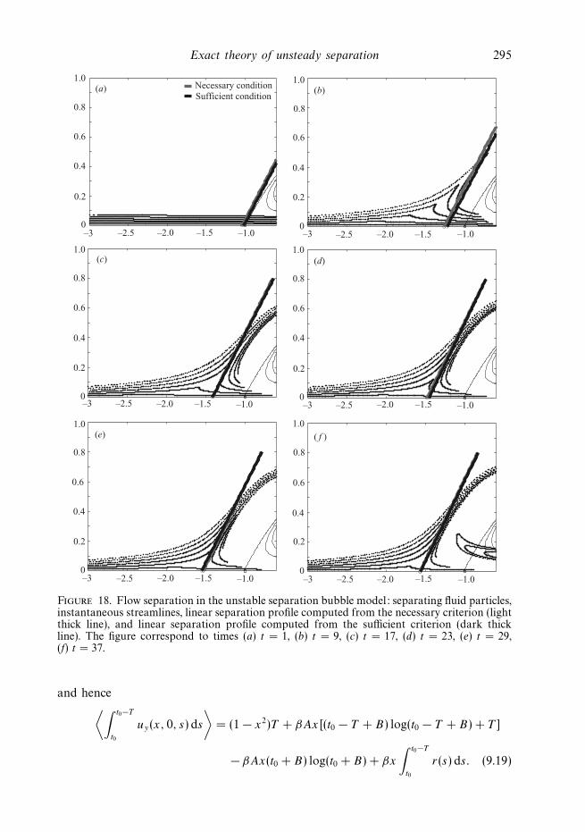
Exact theory of unsteady separation 295

0.8

1.0

0.6

0.4

0.2

0

0.8

1.0

0.6

0.4

0.2

0

0.8

1.0

0.6

0.4

0.2

0

0.8

1.0

0.6

0.4

0.2

0

0.8

1.0

0.6

0.4

0.2

0

0.8

1.0

0.6

0.4

0.2

0

–3 –2.5 –2.0 –1.5 –1.0 –3 –2.5 –2.0 –1.5 –1.0

–3 –2.5 –2.0 –1.5 –1.0

–3 –2.5 –2.0 –1.5 –1.0

–3 –2.5 –2.0 –1.5 –1.0

–3 –2.5 –2.0 –1.5 –1.0

Necessary conditionSufficient condition

(a) (b)

(d)

( f )

(c)

(e)

Figure 18. Flow separation in the unstable separation bubble model: separating fluid particles,instantaneous streamlines, linear separation profile computed from the necessary criterion (lightthick line), and linear separation profile computed from the sufficient criterion (dark thickline). The figure correspond to times (a) t = 1, (b) t = 9, (c) t = 17, (d) t = 23, (e) t = 29,(f) t = 37.

and hence⟨∫ t0−T

t0

uy(x, 0, s) ds

⟩= (1 − x2)T + βAx[(t0 − T + B) log(t0 − T + B) + T ]

− βAx(t0 + B) log(t0 + B) + βx

∫ t0−T

t0

r(s) ds. (9.19)

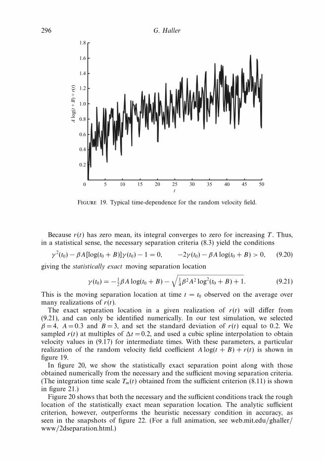
296 G. Haller

0 5 10 15 20 25 30 35 40 45 50

0.2

0.4

0.6

0.8

1.0

1.2

1.4

1.6

1.8

A lo

g(t +

B)

+ r

(t)

t

Figure 19. Typical time-dependence for the random velocity field.

Because r(t) has zero mean, its integral converges to zero for increasing T . Thus,in a statistical sense, the necessary separation criteria (8.3) yield the conditions

γ 2(t0) − βA[log(t0 + B)]γ (t0) − 1 = 0, −2γ (t0) − βA log(t0 + B) > 0, (9.20)

giving the statistically exact moving separation location

γ (t0) = − 12βA log(t0 + B) −

√14β2A2 log2(t0 + B) + 1. (9.21)

This is the moving separation location at time t = t0 observed on the average overmany realizations of r(t).

The exact separation location in a given realization of r(t) will differ from(9.21), and can only be identified numerically. In our test simulation, we selectedβ = 4, A= 0.3 and B = 3, and set the standard deviation of r(t) equal to 0.2. Wesampled r(t) at multiples of �t = 0.2, and used a cubic spline interpolation to obtainvelocity values in (9.17) for intermediate times. With these parameters, a particularrealization of the random velocity field coefficient A log(t + B) + r(t) is shown infigure 19.

In figure 20, we show the statistically exact separation point along with thoseobtained numerically from the necessary and the sufficient moving separation criteria.(The integration time scale Tm(t) obtained from the sufficient criterion (8.11) is shownin figure 21.)

Figure 20 shows that both the necessary and the sufficient conditions track the roughlocation of the statistically exact mean separation location. The analytic sufficientcriterion, however, outperforms the heuristic necessary condition in accuracy, asseen in the snapshots of figure 22. (For a full animation, see web.mit.edu/ghaller/www/2dseparation.html.)

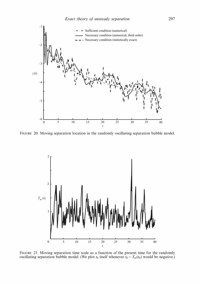
Exact theory of unsteady separation 297

0 5 10 15 20 25 30 35 40–6

–5

–4

–3

–2

–1Sufficient condition (numerical)

Necessary condition (numerical, third order)

Necessary condition (statistically exact)

t

γ (t)

Figure 20. Moving separation location in the randomly oscillating separation bubble model.

0 5 10 15 20 25 30 35 40

1

2

3

t

Tm (t)

Figure 21. Moving separation time scale as a function of the present time for the randomlyoscillating separation bubble model. (We plot t0 itself whenever t0 − Tm(t0) would be negative.)

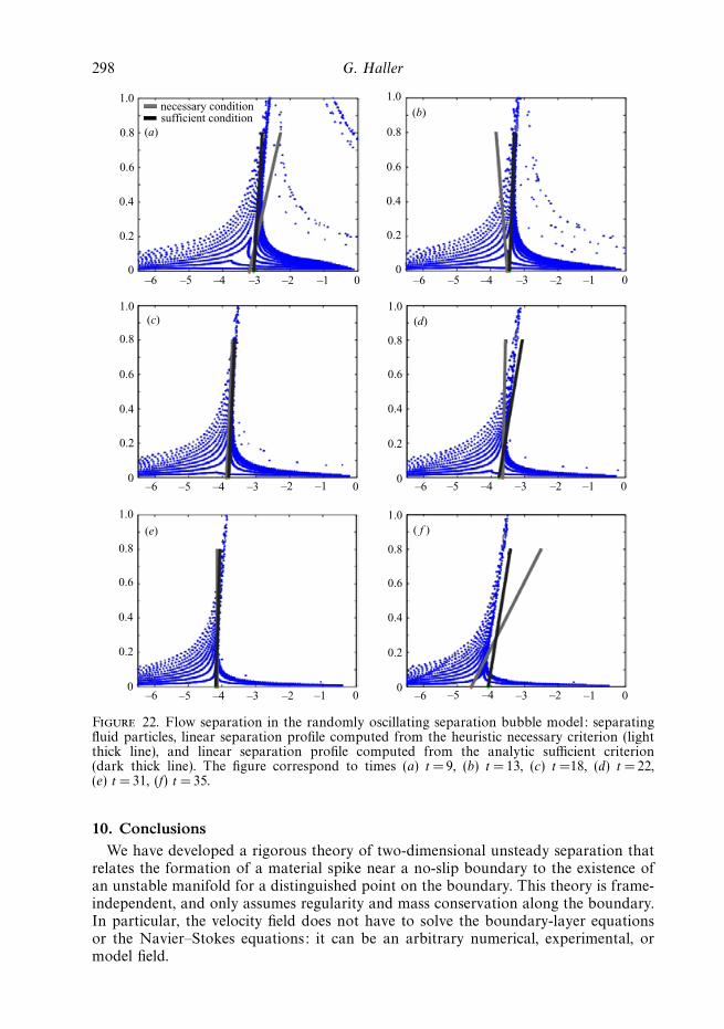
298 G. Haller

necessary conditionsufficient condition

1.0

0.8

0.6

0.4

0.2

0

1.0

0.8

0.6

0.4

0.2

0

1.0

0.8

0.6

0.4

0.2

0

1.0

0.8

0.6

0.4

0.2

0

1.0

0.8

0.6

0.4

0.2

0

1.0

0.8

0.6

0.4

0.2

0–6 –5 –4 –3 –2 –1 0

–6 –5 –4 –3 –2 –1 0

–6 –5 –4 –3 –2 –1 0 –6 –5 –4 –3 –2 –1 0

–6 –5 –4 –3 –2 –1 0

–6 –5 –4 –3 –2 –1 0

(a)

(c)

(e) ( f )

(d)

(b)

Figure 22. Flow separation in the randomly oscillating separation bubble model: separatingfluid particles, linear separation profile computed from the heuristic necessary criterion (lightthick line), and linear separation profile computed from the analytic sufficient criterion(dark thick line). The figure correspond to times (a) t = 9, (b) t = 13, (c) t =18, (d) t = 22,(e) t =31, (f) t = 35.

10. ConclusionsWe have developed a rigorous theory of two-dimensional unsteady separation that

relates the formation of a material spike near a no-slip boundary to the existence ofan unstable manifold for a distinguished point on the boundary. This theory is frame-independent, and only assumes regularity and mass conservation along the boundary.In particular, the velocity field does not have to solve the boundary-layer equationsor the Navier–Stokes equations: it can be an arbitrary numerical, experimental, ormodel field.

Exact theory of unsteady separation 299

The existence of a wall-bound unstable manifold (separation profile) is guaranteedby Prandtl’s classic separation criteria for steady flows with no-slip boundaries. Here,we have extended these criteria to unsteady compressible flows with general timedependence, covering separation and reattachment on fixed and moving boundaries.We have also given an algorithm for computing the shape of the unstable manifold viaa Taylor expansion. This expansion becomes particularly simple for incompressibleflows, for which we have obtained a quartic approximation of the separation profile.

We have also given a theoretical description of moving separation using finite-time invariant manifolds. The two algorithms we described in § 8.1 locate movingseparation and reattachment profiles in incompressible flows with general aperiodictime dependence. As we illustrated in examples, these algorithms are to be used if thefixed or moving nature of separation is a priori unknown.

While motivated by Lagrangian arguments, our criteria are fully Eulerian, andhence do not require the advection of fluid particles. In addition, these criteria onlyuse quantities computed from distributed pressure and skin-friction measurementsalong the wall (cf. § 4), and hence are applicable in active flow control.

Being purely kinematic, our analysis does not distinguish between laminar andturbulent separation. Further work is required, however, on the computationaldifficulties in moving turbulent separation. These difficulties arise from errors inthe long-term numerical integration of our criteria, and from errors in identifying themean component of the backward-time skin-friction integral.

The no-slip assumption (2.2) on the boundary is crucial in our theory, thuscompressible fluids with slip boundary conditions are not covered by the presentresults. The case of slip boundaries is actually simpler to analyse, because we can usethe classic theory of hyperbolic invariant manifolds to describe separation profiles(see Wang et al. 2003).

Beyond the further testing of our results on numerical and experimental velocitydata, a notable challenge is the extension of the theory to three-dimensionalunsteady flows. The Lagrangian definition of separation extends to three dimensions,but technical difficulties arise in the derivation of Eulerian criteria for fixed andmoving unstable manifolds. Some of these difficulties are related to the increaseddimensionality of the problem, whereas others are related to the variety oftopologically different separation profiles that a three-dimensional unsteady flow maysupport. We are addressing these challenges in ongoing work (Grunberg, Surana &Haller 2004).

This work was supported by AFOSR Grant F49620-03-1-0200, and NSF GrantDMS-98-00922. I would like to thank Avi Seifert, Lex Smits, Yong Wang and theanonymous referees for their remarks. I am also grateful to Mohammed-Reza Alam,Olivier Grunberg, Weijiu Liu, Pan Mao and Amit Surana for their close readingof the manuscript, and for all the improvements they suggested. Hayder Salman’snumerical observations and his suggestion of considering the kinematic separationmodel of Ghosh et al. (1998) were very helpful in developing the ideas of this paper.

Appendix AAfter substituting formula (2.20) for f (τ ) in (2.29), we obtain

f1(t) =f1(t0)ρ

2(t)

ρ2(t0)+ ρ2(t)

∫ t

t0

[P (τ, t0) + f0(t0)Q(τ, t0, t) − f 2

0 (t0)bx(τ )

ρ2(t0)

]dτ, (A 1)

300 G. Haller

where

P (τ, t0) =ay(τ )

ρ2(τ )+

ax(τ ) − by(τ )

ρ(τ )

∫ τ

t0

a(s)

ρ(s)ds − bx(τ )

(∫ τ

t0

a(s)

ρ(s)ds

)2

,

Q(τ, t0, t) =1

ρ(t0)

[ax(τ ) − by(τ )

ρ(τ )− 2bx(τ )

∫ τ

t0

a(s)

ρ(s)ds

]. (A 2)

We first observe that for material lines emanating from the separation point (γ, 0)with slopes larger or smaller than the slope of the separation profile, f1(t) will tendto plus or minus infinity, respectively, as t → −∞. This is because in backward time,the separation profile – as any unstable manifold – also repels material lines thatemanate from the separation point, but do not coincide with the separation profile.

As a consequence, for any ε �= 0, (A 1) yields∫ −∞

t0

[P (τ, t0) + [f0(t0) + ε]Q(τ, t0, t) − [f0(t0) + ε]2bx(τ )

ρ2(t0)

]dτ = sign (ε)∞. (A 3)

On the separation profile itself, however, f1(t) remains bounded, i.e.

lim supt → −∞

∣∣∣∣∫ t

t0

[P (τ, t0) + f0(t0)Q(τ, t0, t) − f 2

0 (t0)bx(τ )

ρ2(t0)

]dτ

∣∣∣∣ < ∞. (A 4)

Comparing these two expressions we obtain∫ −∞

t0

[Q(τ, t0, t) − [2f (0t0) + ε]

bx(τ )

ρ2(t0)

]dτ = ∞. (A 5)

By assumptions (2.7)–(2.8), we can write

lim supt → −∞

∣∣∣∣∫ t

t0

[2f0(t0) + ε]bx(τ )

ρ2(t0)dτ

∣∣∣∣ = |2f0(t0) + ε|ρ2(t0)

lim supt → −∞

∣∣∣∣∫ t

t0

vxy(γ, 0, τ ) dτ

∣∣∣∣ < ∞,

(A 6)therefore (A 5) simplifies to ∫ −∞

t0

Q(τ, t0, t) dτ = ∞, (A 7)

or equivalently, ∫ −∞

t0

[ax(τ ) − by(τ )

ρ(τ )− 2bx(τ )

∫ τ

t0

a(s)

ρ(s)ds

]dτ = ∞, (A 8)

as claimed in the necessary separation condition (2.22).To prove (2.30), observe that (A 6) simplifies the boundedness condition (A 4) to

lim supt → −∞

∣∣∣∣∫ t

t0

[P (τ, t0) + f0(t0)Q(τ, t0, t)] dτ

∣∣∣∣ < ∞, (A 9)

which, together with (A 7), implies

limt → −∞

∫ t

t0

[P (τ, t0) + f0(t0)Q(τ, t0, t)] dτ∫ t

t0

Q(τ, t0, t) dτ

= 0. (A 10)

Exact theory of unsteady separation 301

However, this is equivalent to

f0(t0) = − limt → −∞

∫ t

t0

P (τ, t0) dτ∫ t

t0

Q(τ, t0, t) dτ

, (A 11)

which is in turn equivalent to (2.30).

Appendix BComputing the O(y, y2, y3) terms in the incompressible separation equation (3.8)

leads to the set of equations

f 1 = (ax − c)f0 + ay, (B 1)

f 2 = ayy + 2[axy − cy]f0 + [axx − 2cx]f20 + 2[ax − 2c]f1, (B 2)

f 3 = ayyy + (axxx − 3cxx)f30 + 3(axxy − 2cxy)f

20 + 3(axyy − cyy)f0

+ 6(axx − 3cx)f0 f1 + 6(axy − 2cy)f1 + 3(ax − 3c)f2, (B 3)

f 4 = ayyyy + (axxxx − 4cxxx)f40 + 4(axxxy − 3cxxy)f

30 + 6(axxyy − 2cxyy)f

20

+ 4(axyyy − cyyy)f0 + 12(axxx − 4cxx)f20 f1 + 24(axxy − 3cxy)f

20 f1

+ 12(axyy − 2cyy)f1 + 12(axx − 4cx)f21 + 12(axx − 4cx)f0 f2

+ 12(axy − 3cy)f2 + 4(ax − 4c)f3. (B 4)

We note the following incompressibility relations derived from (3.6):

ax + 2c = 0, axy + 3cy = 0, axx + 2cx = 0, (B 5a–c)

axxx + 2cxx = 0, axxy + 3cxy = 0, axyy + 4cyy = 0, (B 5d–f)

axxxx + 2cxxx = 0, axxxy + 3cxxy = 0, (B 5g, h)

axxyy + 4cxyy = 0, axyyy + 5cyyy = 0. (B 5i, j)

We first integrate (B 1), then substitute (3.10) and use (B 5a) to obtain

f1(t) = f1(t0) +

∫ t

t0

[ay(τ ) − 3c(τ )f0(t0) − 3c(τ )

∫ τ

t0

a(s) ds

]dτ (B 6)

for the first-order term in the expansion for the incompressible separation profile. Be-cause f1(t) remains bounded in backward time at a fixed separation point, we can usethe argument of Appendix A to derive (3.16) from (B 6). The expression (3.16) can alsobe obtained by setting b(τ ) ≡ 0 and by(τ ) = c(τ ) in its compressible counterpart (2.30).

Next we integrate (B 2) and observe that the boundedness of f2(t) implies theboundedness of the integral∫ t

t0

[ayy(τ ) − 8cy(τ )f0(τ ) − 4cx(τ )f 2

0 (τ ) − 8c(τ )f1(τ )]dτ (B 7)

for all t � t0. Invoking the arguments of Appendix A, then substituting (B 6) andusing (B 5) leads to (3.17). Again, this result also follows from the compressiblecurvature formula (2.33) if we note that

b = 0, bx = 0, by = c, bxx = 0, bxy = cx, byy = cy, (B 8)

hold for incompressible flows.

302 G. Haller

We now integrate (B 3) and use the incompressibility conditions in (B 5) to find thatthe integral∫ t

t0

[ayyy − 5cxxf

30 − 15cxyf

20 − 15cyyf0 − 30cyf1 − 30cx f0f1 − 15cf2

]dτ (B 9)

must be bounded for all t � t0. Proceeding again as above, we use this boundednessto obtain (3.18). Finally, we integrate (B 4) and follow the same procedure to obtainthe last formula in (3.19).

Appendix CRecall that the flow map associated with (2.1) is defined as

Ftt0(x0, y0) =

(x(t; x0, y0, t0)

y(t; x0, y0, t0)

). (C 1)

The Jacobian of this map, usually called the deformation gradient, is given by theformula

∇Ftt0(x0, y0) =

∂x(t)

∂x0

∂x(t)

∂y0

∂y(t)

∂x0

∂y(t)

∂y0

. (C 2)

If u and v are continuously differentiable, then the entries of the matrix ∇Ftt0

remainbounded on bounded domains for any finite t (cf. Arnold 1978). In view of this, theformula

det ∇Ftt0

=∂x(t)

∂x0

∂y(t)

∂y0

− ∂x(t)

∂y0

∂y(t)

∂x0

(C 3)

and Van Dommelen’s condition (2.39) together imply

det ∇Ftt0(γ, η) = 0. (C 4)

This last equation, however, contradicts Liouville’s formula

det ∇Ftt0(γ, η) = exp

(∫ t

t0

∇ · v(x(s; γ, η, t0), y(s; γ, η, t0), s) ds

), (C 5)

for continuously differentiable velocity fields (cf. Arnold 1978). Therefore, v = (u, v)cannot be continuously differentiable.

To find an exact Lagrangian criterion for fixed unsteady separation at a boundarypoint, we differentiate (2.1) with respect to the initial positions (x0, y0) to obtain thematrix differential equation

d

dt∇Ft

t0(x0, y0) =

(ux

(Ft

t0(x0, y0), t

)uy

(Ft

t0(x0, y0), t

)vx

(Ft

t0(x0, y0), t

)vy

(Ft

t0(x0, y0), t

))

∇Ftt0(x0, y0), (C 6)

with the initial condition

∇Ftt0(x0, y0) =

(1 0

0 1

). (C 7)

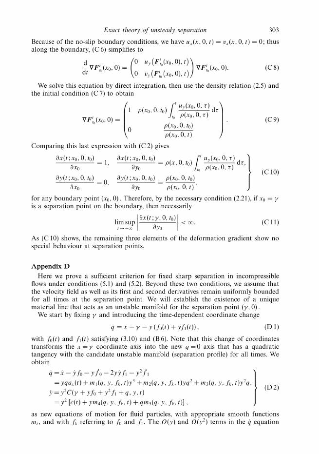
Exact theory of unsteady separation 303

Because of the no-slip boundary conditions, we have ux(x, 0, t) = vx(x, 0, t) = 0; thusalong the boundary, (C 6) simplifies to

d

dt∇Ft

t0(x0, 0) =

(0 uy

(Ft

t0(x0, 0), t

)0 vy

(Ft

t0

(x0, 0), t

))

∇Ftt0(x0, 0). (C 8)

We solve this equation by direct integration, then use the density relation (2.5) andthe initial condition (C 7) to obtain

∇Ftt0(x0, 0) =

1 ρ(x0, 0, t0)

∫ t

t0

uy(x0, 0, τ )

ρ(x0, 0, τ )dτ

0ρ(x0, 0, t0)

ρ(x0, 0, t)

. (C 9)

Comparing this last expression with (C 2) gives

∂x(t; x0, 0, t0)

∂x0

= 1,∂x(t; x0, 0, t0)

∂y0

= ρ(x, 0, t0)

∫ t

t0

uy(x0, 0, τ )

ρ(x0, 0, τ )dτ,

∂y(t; x0, 0, t0)

∂x0

= 0,∂y(t; x0, 0, t0)

∂y0

=ρ(x0, 0, t0)

ρ(x0, 0, t),

(C 10)

for any boundary point (x0, 0) . Therefore, by the necessary condition (2.21), if x0 = γ

is a separation point on the boundary, then necessarily

lim supt → −∞

∣∣∣∣∂x(t; γ, 0, t0)

∂y0

∣∣∣∣ < ∞. (C 11)

As (C 10) shows, the remaining three elements of the deformation gradient show nospecial behaviour at separation points.

Appendix DHere we prove a sufficient criterion for fixed sharp separation in incompressible

flows under conditions (5.1) and (5.2). Beyond these two conditions, we assume thatthe velocity field as well as its first and second derivatives remain uniformly boundedfor all times at the separation point. We will establish the existence of a uniquematerial line that acts as an unstable manifold for the separation point (γ, 0) .

We start by fixing γ and introducing the time-dependent coordinate change

q = x − γ − y (f0(t) + yf1(t)) , (D 1)

with f0(t) and f1(t) satisfying (3.10) and (B 6). Note that this change of coordinatestransforms the x = γ coordinate axis into the new q =0 axis that has a quadratictangency with the candidate unstable manifold (separation profile) for all times. Weobtain

q = x − yf0 − yf 0 − 2yyf1 − y2f 1

= yqax(t) + m1(q, y, fk, t)y3 + m2(q, y, fk, t)yq2 + m3(q, y, fk, t)y

2q,

y = y2C(γ + yf0 + y2f1 + q, y, t)

= y2 [c(t) + ym4(q, y, fk, t) + qm5(q, y, fk, t)] ,

(D 2)

as new equations of motion for fluid particles, with appropriate smooth functionsmi, and with fk referring to f0 and f1. The O(y) and O(y2) terms in the q equation

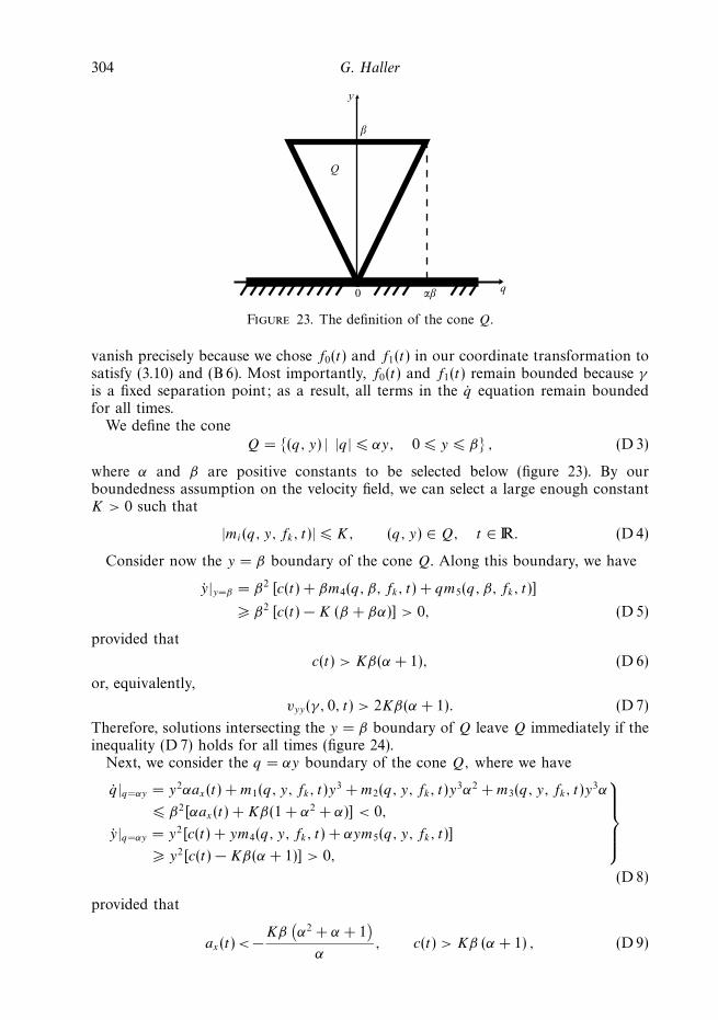
304 G. Haller

y

Q

q0 αβ

β

Figure 23. The definition of the cone Q.

vanish precisely because we chose f0(t) and f1(t) in our coordinate transformation tosatisfy (3.10) and (B 6). Most importantly, f0(t) and f1(t) remain bounded because γ

is a fixed separation point; as a result, all terms in the q equation remain boundedfor all times.

We define the cone

Q = {(q, y) | |q| � αy, 0 � y � β} , (D 3)

where α and β are positive constants to be selected below (figure 23). By ourboundedness assumption on the velocity field, we can select a large enough constantK > 0 such that

|mi(q, y, fk, t)| � K, (q, y) ∈ Q, t ∈ �. (D 4)

Consider now the y = β boundary of the cone Q. Along this boundary, we have

y|y=β = β2 [c(t) + βm4(q, β, fk, t) + qm5(q, β, fk, t)]

� β2 [c(t) − K (β + βα)] > 0, (D 5)

provided that

c(t) > Kβ(α + 1), (D 6)

or, equivalently,

vyy(γ, 0, t) > 2Kβ(α + 1). (D 7)

Therefore, solutions intersecting the y = β boundary of Q leave Q immediately if theinequality (D 7) holds for all times (figure 24).

Next, we consider the q = αy boundary of the cone Q, where we have

q|q=αy = y2αax(t) + m1(q, y, fk, t)y3 + m2(q, y, fk, t)y

3α2 + m3(q, y, fk, t)y3α

� β2[αax(t) + Kβ(1 + α2 + α)] < 0,

y|q=αy = y2[c(t) + ym4(q, y, fk, t) + αym5(q, y, fk, t)]

� y2[c(t) − Kβ(α + 1)] > 0,

(D 8)

provided that

ax(t) < −Kβ(α2 + α + 1

)α

, c(t) > Kβ (α + 1) , (D 9)

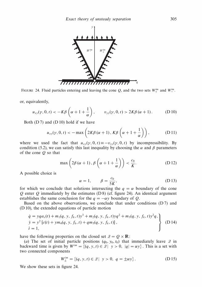
Exact theory of unsteady separation 305

y

q

W im– W im

+

Figure 24. Fluid particles entering and leaving the cone Q, and the two sets W im+ and W im

− .

or, equivalently,

uxy(γ, 0, t) < −Kβ

(α + 1 +

1

α

), vyy(γ, 0, t) > 2Kβ (α + 1) . (D 10)

Both (D 7) and (D 10) hold if we have

uxy(γ, 0, t) < − max

(2Kβ (α + 1) , Kβ

(α + 1 +

1

α

)), (D 11)

where we used the fact that uxy(γ, 0, t) ≡ −vyy(γ, 0, t) by incompressibility. Bycondition (5.2), we can satisfy this last inequality by choosing the α and β parametersof the cone Q so that

max

(2β (α + 1) , β

(α + 1 +

1

α

))<

c0

K. (D 12)

A possible choice is

α = 1, β =c0

5K, (D 13)

for which we conclude that solutions intersecting the q = α boundary of the coneQ enter Q immediately by the estimates (D 8) (cf. figure 24). An identical argumentestablishes the same conclusion for the q = −αy boundary of Q.

Based on the above observations, we conclude that under conditions (D 7) and(D 10), the extended equations of particle motion

q = yqax(t) + m1(q, y, fk, t)y3 + m2(q, y, fk, t)yq2 + m3(q, y, fk, t)y

2q,

y = y2 [c(t) + ym4(q, y, fk, t) + qm5(q, y, fk, t)] ,

t = 1,

(D 14)

have the following properties on the closed set Q = Q × �:(a) The set of initial particle positions (q0, y0, t0) that immediately leave Q in

backward time is given by Wim = {(q, y, t) ∈ Q | y > 0, |q| = αy} . This is a set withtwo connected components

Wim± = {(q, y, t) ∈ Q | y > 0, q = ±αy} . (D 15)

We show these sets in figure 24.

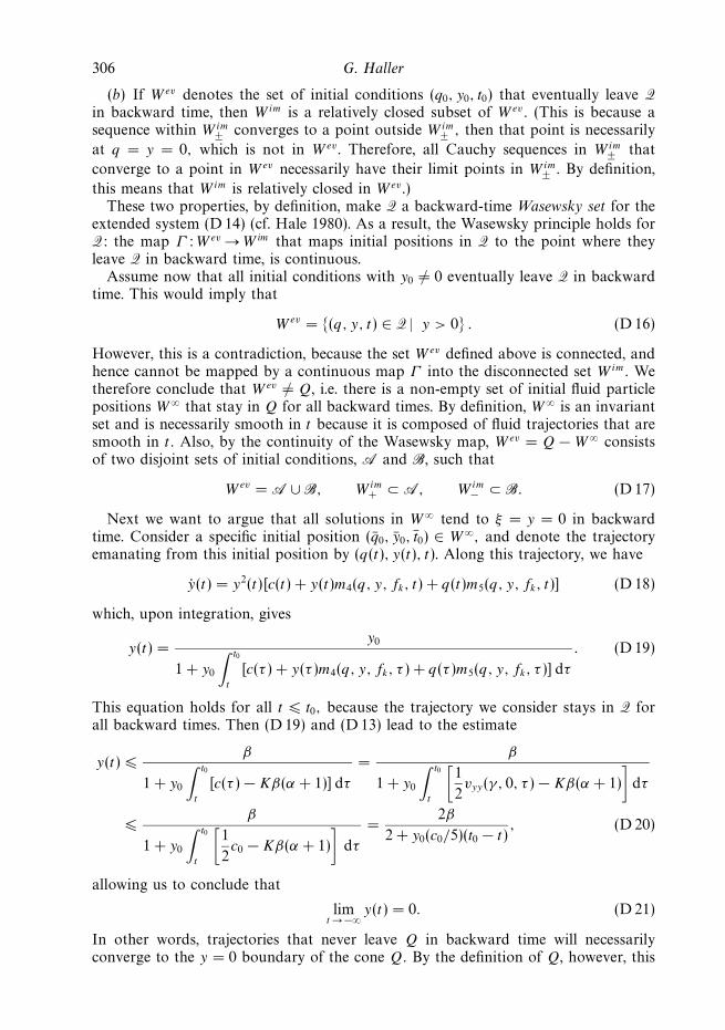
306 G. Haller

(b) If Wev denotes the set of initial conditions (q0, y0, t0) that eventually leave Qin backward time, then Wim is a relatively closed subset of Wev. (This is because asequence within Wim

± converges to a point outside Wim± , then that point is necessarily

at q = y = 0, which is not in Wev . Therefore, all Cauchy sequences in Wim± that

converge to a point in Wev necessarily have their limit points in Wim± . By definition,

this means that Wim is relatively closed in Wev .)These two properties, by definition, make Q a backward-time Wasewsky set for the

extended system (D14) (cf. Hale 1980). As a result, the Wasewsky principle holds forQ: the map Γ : Wev → W im that maps initial positions in Q to the point where theyleave Q in backward time, is continuous.

Assume now that all initial conditions with y0 �= 0 eventually leave Q in backwardtime. This would imply that

Wev = {(q, y, t) ∈ Q | y > 0} . (D 16)

However, this is a contradiction, because the set Wev defined above is connected, andhence cannot be mapped by a continuous map Γ into the disconnected set Wim. Wetherefore conclude that Wev �= Q, i.e. there is a non-empty set of initial fluid particlepositions W ∞ that stay in Q for all backward times. By definition, W ∞ is an invariantset and is necessarily smooth in t because it is composed of fluid trajectories that aresmooth in t. Also, by the continuity of the Wasewsky map, Wev = Q − W∞ consistsof two disjoint sets of initial conditions, A and B, such that

Wev = A ∪ B, W im+ ⊂ A, W im

− ⊂ B. (D 17)

Next we want to argue that all solutions in W∞ tend to ξ = y = 0 in backwardtime. Consider a specific initial position (q0, y0, t0) ∈ W ∞, and denote the trajectoryemanating from this initial position by (q(t), y(t), t). Along this trajectory, we have

y(t) = y2(t)[c(t) + y(t)m4(q, y, fk, t) + q(t)m5(q, y, fk, t)] (D 18)

which, upon integration, gives

y(t) =y0

1 + y0

∫ t0

t

[c(τ ) + y(τ )m4(q, y, fk, τ ) + q(τ )m5(q, y, fk, τ )] dτ

. (D 19)

This equation holds for all t � t0, because the trajectory we consider stays in Q forall backward times. Then (D 19) and (D13) lead to the estimate

y(t) �β

1 + y0

∫ t0

t

[c(τ ) − Kβ(α + 1)] dτ

=β

1 + y0

∫ t0

t

[1

2vyy(γ, 0, τ ) − Kβ(α + 1)

]dτ

�β

1 + y0

∫ t0

t

[1

2c0 − Kβ(α + 1)

]dτ

=2β

2 + y0(c0/5)(t0 − t), (D 20)

allowing us to conclude that

limt → −∞

y(t) = 0. (D 21)

In other words, trajectories that never leave Q in backward time will necessarilyconverge to the y = 0 boundary of the cone Q. By the definition of Q, however, this

Exact theory of unsteady separation 307

convergence in the y-direction implies

limt → −∞

q(t) = 0. (D 22)

We therefore conclude that all trajectories in W∞ converge to y = q =0 in backwardtime, thus W ∞ is an unstable manifold for (γ, 0). Any material curve in thismanifold admits bounded and unique y derivatives according to formulae (3.16)–(3.19), therefore the unstable manifold is unique up to terms of order O(y3).

The same argument applies when higher-order terms of the candidate separationprofile (3.15) are included in the initial coordinate change (D1), leading to a uniqueunstable manifold up to terms of order O(yn). Here, n is an arbitrary integer thatcan be as large as the degree of differentiability of the original velocity field.

Given the existence of the separation profile, we only need to argue that theseparation is indeed sharp along this profile. To prove sharp separation, it is enoughto establish that the y-coordinate of fluid particles in the separation profile W ∞ growsmonotonically for all times as long as the particles are in a vicinity of the boundary.Note that W ∞ has been constructed as a material line whose y � β portion is fullycontained in the cone Q. For all fluid particles that lie in the separation profile aswell as in the {0 < y � β} neighbourhood of the boundary, (D 2) and (D 13) yieldthe estimate

y = y2 [c(t) + ym4(q, y, fk, t) + qm5(q, y, fk, t)]

� y2[

12c0 − Kβ(α + 1)

]� y2(c0/10). (D 23)

Therefore, the y-coordinate of fluid particles in W∞ grows monotonically in the{0 < y � β} neighbourhood of the boundary, resulting in sharp separation.

Appendix EHere we show that for general incompressible flows, (8.11) gives a sufficient

condition for finite-time sharp separation close to the moving effective separationpoint γeff (t, t0). We shall show this by arguing that if γeff (t, t0) moves slowly enough fort ∈ [t0 − Tm(t0), t0], then any point (γ, 0) close enough to γeff (t, t0) acts as a separationpoint in the Lagrangian frame over that time interval. From this argument, we obtaina set of points that can be considered finite-time separation points. The size of thisset tends to zero as the admissible time scale Tm(t0) increases. As a result, in numericalcalculations we obtain a separation point that is unique for practical purposes.

We start by selecting a boundary point (γ, 0) and introducing a time-dependentcoordinate change

q = x − γ − yφ(t), (E 1)

with φ(t) to be defined below. We obtain the transformed velocity field

q = x − yφ − yφ

= y(a − φ) + yqax + y2[(ax − c)φ + ay]

+ (l1y3 + l2y

2q + l3yq2)(l4 + n1φ),

y = y2C(γ + yφ, y, t)

= y2[c(t) + (l5y + l6q)(l7 + n2φ)],

(E 2)

with appropriate smooth functions lj (q, y, φ, t) and nk(q, y, φ, t). These functionsare typically not globally bounded in φ, thus they will grow unbounded if φ growsunbounded in time.

308 G. Haller

If we select φ(t) to satisfy

φ = a, (E 3)

then the O(y) term in the q equation of (E 2) vanishes. By our assumptions, the O(yq)term remains bounded regardless of the choice of φ. If γ were a fixed separationpoint, then the solution φ(t) of (E 3) would remain bounded for all times, and hencethe O(y3, y2q, yq2) terms in the q equation would also remain bounded for all times.However, γ is not a fixed separation point in our current setting, and hence theO(y3, y2q, yq2) terms in the q equation will typically grow unbounded in time.

To control the above-mentioned growth of nonlinear terms in (E 2), we select

γ = γeff (t, t0) + �(t, t0), (E 4)

with γeff (t, t0) denoting an effective separation point. In that case, by the mean-valuetheorem, any solution of (E 3) can be written as

φ(t) = φ(t0) +

∫ t

t0

A(γ, 0, τ ) dτ = φ(t0) +

∫ t

t0

A(γeff (t, t0) + �(t, t0), 0, τ ) dτ

= φ(t0) +

∫ t

t0

[A(γeff (t, t0), 0, τ ) + Ax(γ

∗(τ ), 0, τ )�(t, t0)]dτ

= φ(t0) + �(t, t0)

∫ t

t0

uxy(γ∗(τ ), 0, τ ) dτ, (E 5)

for some γ ∗(τ ) falling between γ and γeff (t, t0).Let I (t, t0) denote the maximal x interval covered by the moving effective separation

point γeff (s, t0) while s varies over the time interval [t, t0] . We denote the length ofI (t, t0) by δ(t, t0). If we select γ as in (8.10), then for any t < t0, we have the estimate

|φ(t)| =

∣∣∣∣φ(t0) + �(t, t0)

∫ t

t0

uxy(γ∗(τ ), 0, τ ) dτ

∣∣∣∣� |φ(t0)| + δ(t, t0)

∣∣∣∣∫ t

t0

uxy(γ∗(τ ), 0, τ ) dτ

∣∣∣∣� |φ(t0)| + δ(t, t0)

∫ t0

t

maxx∈I (t,t0)

|uxy(x, 0, τ )|dτ. (E 6)

As in Appendix D, we now define the cone

Q = {(q, y) | |q| � αy, 0 � y � β} , (E 7)

where α and β are positive constants to be selected below. Modifying the functions ljand nkφ in (E 2) smoothly outside a time interval [t0 −Tm, t0] with Tm to be determinedbelow, we can select a constant K > 0 such that the modified functions satisfy

|lj (q, y, φ, t)| , |nk(q, y, φ, t)φ| � K, (q, y) ∈ Q, t ∈ �. (E 8)

Along the y = β boundary, we now have

y|y=β = β2[c(t) + (l5y + l6q)(l7 + n2φ)]

� β2[c(t) − 2K2(β + βα)] > 0, (E 9)

provided that

c(t) > 2K2β(1 + α), (E 10)

Exact theory of unsteady separation 309

or, equivalently,

vyy(γ, 0, t) > 4K2β(1 + α). (E 11)

Therefore, solutions intersecting the y = β boundary of Q leave Q immediately if theinequality (E 11) holds for all times.

Next we consider the q = αy boundary of the cone Q, where we have

q|q=αy = y2[αax(t) + (ax − c)φ + ay + y(l1 + l2α + l3α2)(l4 + n1φ)] < 0,

y|q=αy = y2[c(t) + y(l5 + l6α)(l7 + n2φ)] > 0,

}(E 12)

provided that

αax(t) + (ax − c)φ + ay < −2K2β(1 + α + α2),

c(t) > 2K2β(1 + α).

}(E 13)

For fixed α > 0, we can always select an appropriately small β > 0 such that both ofthese inequalities hold, provided that

αax(t) + 32|ax(t)|

[|φ(t0)| + δ(t, t0)

∫ t0

t

maxx∈I (t,t0)

|uxy(x, 0, τ )| dτ

]+ |ay(t)| < 0,

c(t) > 0,

(E 14)

where we used the incompressibility relation ax + 2c = 0.The conditions in (E 14) hold if we require

δ(t, t0)

∫ t0

t

maxx∈I (t,t0)

|uxy(x, 0, τ )| dτ < 23

[α − max

x∈I (t,t0)

|uyy(x, 0, t)|2|uxy(x, 0, t)|

]− |φ(t0)|,

maxx∈I (t,t0)

uxy(x, 0, t) < 0,

(E 15)

Recall that α denotes the tangent of the half-angle of the cone Q, and φ(t0) denotesthe tangent of the angle at which Q is tilted relative to the vertical in the original (x,

y) coordinate system.Our selection of the parameters α and φ(t0) will depend on the given problem.

Ideally, φ(t0) should be chosen as the tangent of a mean value of the separation angle,and α should be chosen as the tangent of the maximal deviation of the separationangle from its mean value. To obtain a universal estimate, we select

α = 3 + maxx∈I (t,t0)

|uyy(x, 0, t)|2 |uxy(x, 0, t)| + 3

2|φ(t0)| , (E 16)

which will still accommodate sizable variations in the separation angle. (For specificproblems, more refined choices of α may be possible.) For the above choice ofα, the conditions (E 15) are equivalent to (8.11). Under these conditions, solutionsintersecting the q = α boundary of the cone Q enter the cone immediately by theestimates (D 8).

With this last conclusion, the rest of our argument is identical to that of AppendixD. Following that argument, we find that γ is a fixed sharp separation point forthe modified system that admits all the uniform bounds that we have assumed. Asa result, the original unmodified system also admits sharp finite-time separation atγ as long as it agrees with the modified system. The resulting separation profile,however, is non-unique, which is a common feature of finite-time separation points.As a result, the choice (E 16) will give a separation profile, but not necessarily theone that ejects particles the most intensely. In particular problems, we may improveupon this conservative choice of parameters by picking a different α in (E 16).

310 G. Haller

REFERENCES

Arnold, V. I. 1978 Ordinary Differential Equations. MIT Press.

Cassel, K. W., Smith, F. T. & Walker, J. D. A. 1996 The onset of instability in unsteadyboundary-layer separation. J. Fluid Mech. 315, 223–256.

Cowley, S. J. 1983 Computer extension and analytic continuation of Blasius’ expansion for impulsiveflow past a circular cylinder. J. Fluid. Mech. 135, 389–405.

Cowley, S. J., Van Dommelen, L. L. & Lam, S. T. 1990 On the use of Lagrangian variables in thedescription of unsteady boundary-layer separation. Phil. Trans. R. Soc. Lond. A 333, 348–378.

Degani, A. T., Walker, J. D. A. & Smith, F. T. 1998 Unsteady separation past moving surfaces.J. Fluid. Mech. 375, 1–38.

Friedlander, S. & Vishik, M. M. 1991 Instability criteria for the flow of an inviscid incompressiblefluid. Phys. Rev. Lett. 66, 2204–2206.

Ghosh, S., Leonard, A. & Wiggins, S. 1998 Diffusion of a passive scalar from a no-slip boundaryinto a two-dimensional chaotic advection field. J. Fluid Mech. 372, 119–163.

Grunberg, O., Surana, A. & Haller, G. 2004 Three-dimensional unsteady separation: a kinematictheory. Preprint.

Hackborn, W. W., Ulucakli, M. E. & Yuster, T. 1997 A theoretical and experimental study ofhyperbolic and degenerate mixing regions in chaotic Stokes flow. J. Fluid Mech. 346, 23–48.

Hale, J. K. 1980 Ordinary Differential Equations. Krieger, Malabar, FL.

Haller, G. & Poje, A. 1998 Finite-time transport in aperiodic flows. Physica D 119, 352–380.

Haller, G. 2000 Finding finite-time invariant manifolds in two-dimensional velocity fields. Chaos10, 99–108.

Haller, G. 2001 Lagrangian structures and the rate of strain in two-dimensional turbulence. Phys.Fluids A 13, 3365–3385.

Lifshitz, A. 1991 Essential spectrum and local stability conditions in hydrodynamics. Phys. Lett.A 152, 199–204.

Lighthill, M. J. 1963 Boundary layer theory. In Laminar Boundary Layers (ed. L. Rosenhead).Dover.

Liu, C. S. & Wan, Y.-H. 1985 A simple exact solution of the Prandtl boundary layer equationscontaining a point of separation, Arch. Rat. Mech. Anal. 89, 177–185.

Lugt, H. 1995 Vortex Flow in Nature and Technology. Krieger, Malabar, FL.

Moore, F. K. 1958 On the separation of unsteady boundary layer. In Boundary-layer Research(ed. H. Gortler) pp. 296–311. Springer.

Peridier, V. J. 1995 A Lagrangian scheme for the animation of unsteady separation. ComputersFluids 24, 269–291.

Perry, A. E. & Chong, M. S. 1986 A series expansion study of the Navier–Stokes equations withapplications to three-dimensional separation patterns. J. Fluid Mech. 173, 207–223.

Prandtl, L. 1904 Uber Flussigkeitsbewegung bei sehr kleiner Reibung. Verh. III, Int. Math. Kongr.,Heidelberg pp. 484–491.

Rott, N. 1956 Unsteady viscous flows in the vicinity of a separation point. Q. Appl. Maths 13,444–451.

Schlichting, H. & Gersten, K. 2000 Boundary Layer Theory (8th edn) Springer.

Sears, W. R. & Tellionis, D. P. 1971 Unsteady boundary layer separation. In Recent Research onUnsteady Boundary Layers (ed. E. Eichelbrenner), pp. 404–447.

Sears, W. R. & Tellionis, D. P. 1975 Boundary-layer separation in unsteady flow. SIAM J. Appl.Maths 28 215–235.

Shariff, K., Pulliam, T. H. & Ottino, J. M. 1991 A dynamical systems analysis of kinematics inthe time-periodic wake of a circular cylinder. Lect. Appl. Math. 28, 613–646.

Sobey, I. J. 2000 Introduction to Interactive Boundary Layer Theory. Oxford University Press.

Tritton, D. J. 1988 Physical Fluid Dynamics. Oxford University Press.

Van Dommelen, L. L. 1981 Unsteady Boundary Layer Separation. PhD thesis, Cornell University,Ithaca, NY.

Van Dommelen, L. L. & Cowley, S. J. 1990 On the Lagrangian description of unsteady boundarylayer separation. Part 1. General theory. J. Fluid Mech. 210, 593–626.

Van Dommelen, L. L. & Shen, S. F. 1982 The genesis of separation. In Numerical and PhysicalAspects of Aerodynamics Flow (ed. T. Cebici) pp. 283–311. Long Beach, California.

Exact theory of unsteady separation 311

Wang, Y., Haller, G., Banaszuk, A. & Tadmor, G. 2003 Closed-loop Lagrangian separationcontrol in a bluff body shear flow model. Phys. Fluids A 15, 2251–2266.

Williams, J. C. 1977 Incompressible boundary layer separation. Annu. Rev. Fluid. Mech. 9, 113–144.

Wu, J. Z., Tramel, R. W., Zhu, F. L. & Yin, X. Y. 2000 A vorticity dynamics theory of three-dimensional flow separation. Phys. Fluids A 12, 1932–1954.

Yuster, T. & Hackborn, W. W. 1997 On invariant manifolds attached to oscillating boundaries ofStokes flows. Chaos 7, 769–776.