Embed Size (px)
Citation preview
Unsupervised learning in NLP (INLP ch. 5)
CS 685, Spring 2021Advanced Topics in Natural Language Processing
http://brenocon.com/cs685https://people.cs.umass.edu/~brenocon/cs685_s21/
Brendan O’ConnorCollege of Information and Computer Sciences
University of Massachusetts Amherst
WSD: do context words naturally cluster?
2
96 CHAPTER 5. LEARNING WITHOUT SUPERVISION
0 10 20 30 40density of word group 1
0
20
40
density
ofword
gro
up
2
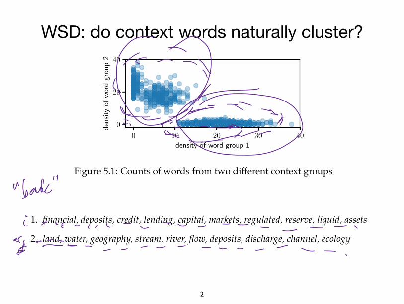
Figure 5.1: Counts of words from two different context groups
bank, the immediate context might typically include words from one of the following twogroups:
1. financial, deposits, credit, lending, capital, markets, regulated, reserve, liquid, assets
2. land, water, geography, stream, river, flow, deposits, discharge, channel, ecology
Now consider a scatterplot, in which each point is a document containing the word bank.The location of the document on the x-axis is the count of words in group 1, and thelocation on the y-axis is the count for group 2. In such a plot, shown in Figure 5.1, two“blobs” might emerge, and these blobs correspond to the different senses of bank.
Here’s a related scenario, from a different problem. Suppose you download thousandsof news articles, and make a scatterplot, where each point corresponds to a document:the x-axis is the frequency of the group of words (hurricane, winds, storm); the y-axis is thefrequency of the group (election, voters, vote). This time, three blobs might emerge: onefor documents that are largely about a hurricane, another for documents largely about aelection, and a third for documents about neither topic.
These clumps represent the underlying structure of the data. But the two-dimensionalscatter plots are based on groupings of context words, and in real scenarios these wordlists are unknown. Unsupervised learning applies the same basic idea, but in a high-dimensional space with one dimension for every context word. This space can’t be di-rectly visualized, but the goal is the same: try to identify the underlying structure of theobserved data, such that there are a few clusters of points, each of which is internallycoherent. Clustering algorithms are capable of finding such structure automatically.
5.1.1 K-means clustering
Clustering algorithms assign each data point to a discrete cluster, zi 2 1, 2, . . .K. One ofthe best known clustering algorithms is K-means, an iterative algorithm that maintains
Jacob Eisenstein. Draft of November 13, 2018.
96 CHAPTER 5. LEARNING WITHOUT SUPERVISION
Figure 5.1: Counts of words from two different context groups
bank, the immediate context might typically include words from one of the following twogroups:
1. financial, deposits, credit, lending, capital, markets, regulated, reserve, liquid, assets
2. land, water, geography, stream, river, flow, deposits, discharge, channel, ecology
Now consider a scatterplot, in which each point is a document containing the word bank.The location of the document on the x-axis is the count of words in group 1, and thelocation on the y-axis is the count for group 2. In such a plot, shown in Figure 5.1, two“blobs” might emerge, and these blobs correspond to the different senses of bank.
Here’s a related scenario, from a different problem. Suppose you download thousandsof news articles, and make a scatterplot, where each point corresponds to a document:the x-axis is the frequency of the group of words (hurricane, winds, storm); the y-axis is thefrequency of the group (election, voters, vote). This time, three blobs might emerge: onefor documents that are largely about a hurricane, another for documents largely about aelection, and a third for documents about neither topic.
These clumps represent the underlying structure of the data. But the two-dimensionalscatter plots are based on groupings of context words, and in real scenarios these wordlists are unknown. Unsupervised learning applies the same basic idea, but in a high-dimensional space with one dimension for every context word. This space can’t be di-rectly visualized, but the goal is the same: try to identify the underlying structure of theobserved data, such that there are a few clusters of points, each of which is internallycoherent. Clustering algorithms are capable of finding such structure automatically.
5.1.1 K-means clustering
Clustering algorithms assign each data point to a discrete cluster, zi 2 1, 2, . . .K. One ofthe best known clustering algorithms is K-means, an iterative algorithm that maintains
Jacob Eisenstein. Draft of November 13, 2018.
bank
i ee a a
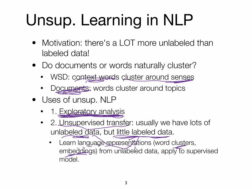
• Motivation: there's a LOT more unlabeled than labeled data!
• Do documents or words naturally cluster? • WSD: context words cluster around senses • Documents: words cluster around topics
• Uses of unsup. NLP • 1. Exploratory analysis • 2. Unsupervised transfer: usually we have lots of
unlabeled data, but little labeled data. • Learn language representations (word clusters,
embeddings) from unlabeled data, apply to supervised model.
3
Unsup. Learning in NLP
of
t
A few methods
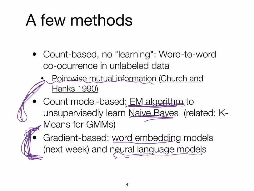
• Count-based, no "learning": Word-to-word co-ocurrence in unlabeled data
• Pointwise mutual information (Church and Hanks 1990)
• Count model-based: EM algorithm to unsupervisedly learn Naive Bayes (related: K-Means for GMMs)
• Gradient-based: word embedding models (next week) and neural language models
4
tI E
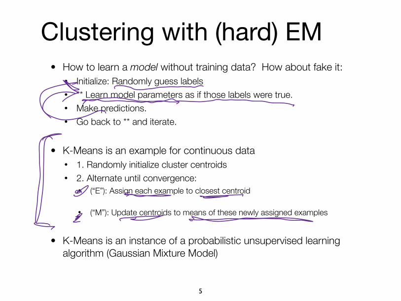
Clustering with (hard) EM• How to learn a model without training data? How about fake it:
• Initialize: Randomly guess labels • ** Learn model parameters as if those labels were true. • Make predictions. • Go back to ** and iterate.
• K-Means is an example for continuous data • 1. Randomly initialize cluster centroids • 2. Alternate until convergence:
• (“E”): Assign each example to closest centroid
• (“M”): Update centroids to means of these newly assigned examples
• K-Means is an instance of a probabilistic unsupervised learning algorithm (Gaussian Mixture Model)
5
F
I
6
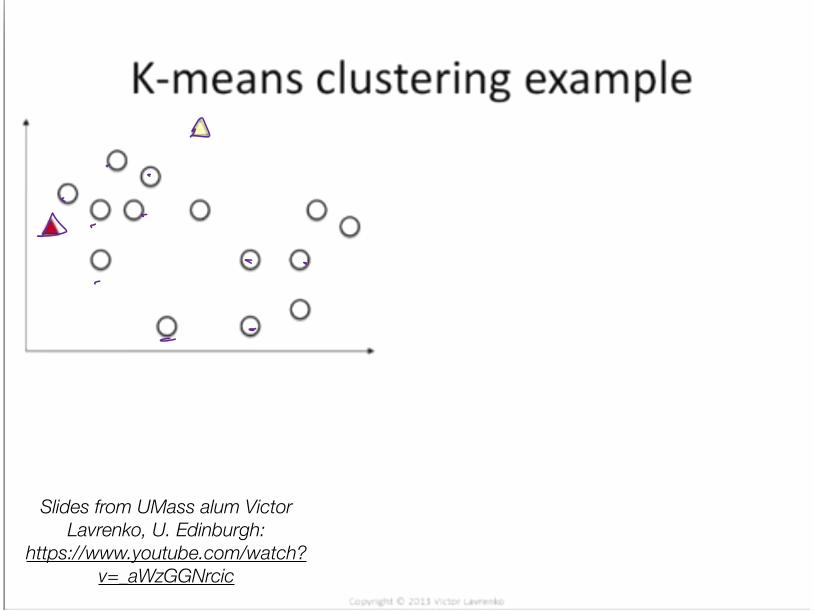
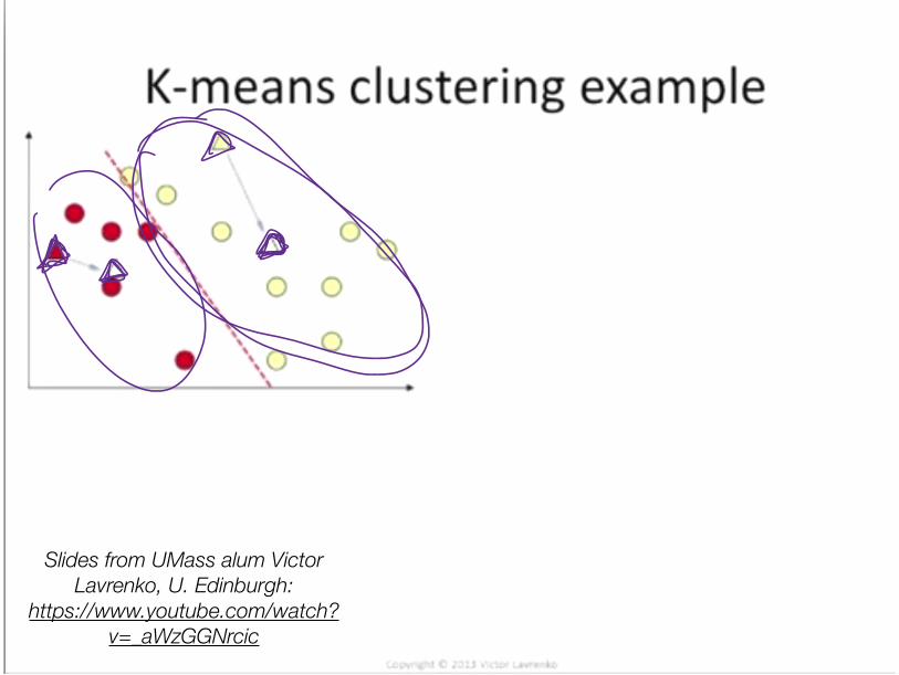
Slides from UMass alum Victor Lavrenko, U. Edinburgh:
https://www.youtube.com/watch?v=_aWzGGNrcic
A
a
7
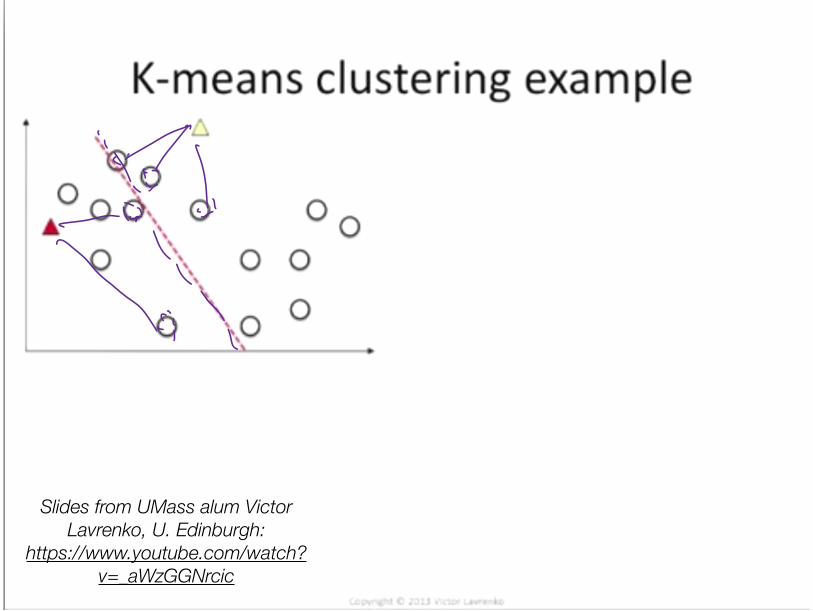
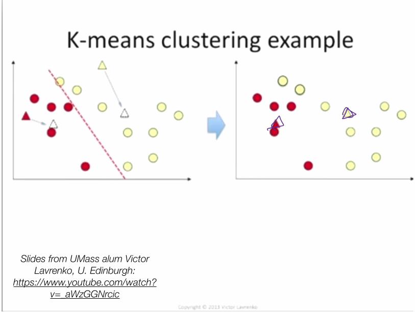
Slides from UMass alum Victor Lavrenko, U. Edinburgh:
https://www.youtube.com/watch?v=_aWzGGNrcic
8
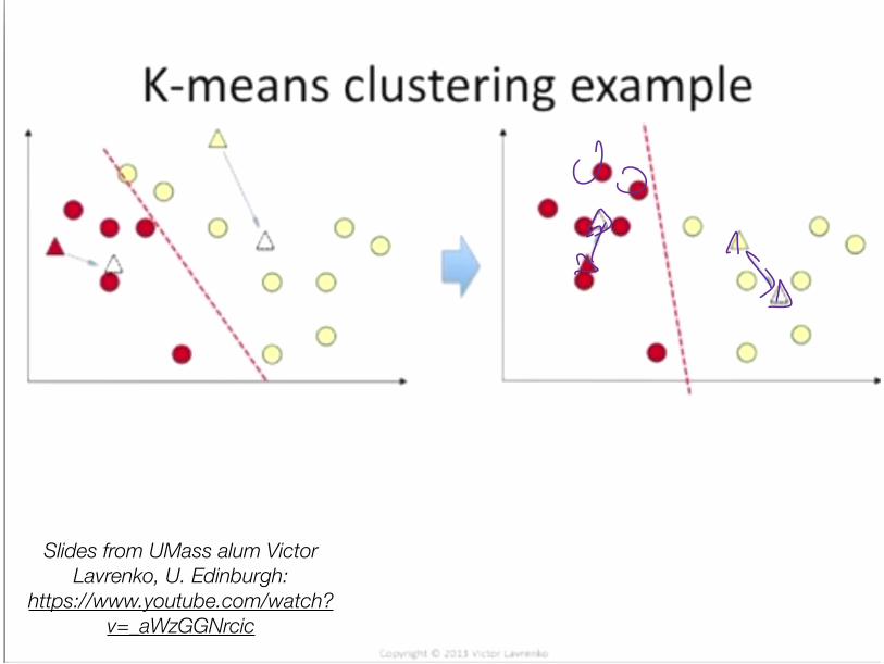
Slides from UMass alum Victor Lavrenko, U. Edinburgh:
https://www.youtube.com/watch?v=_aWzGGNrcic
9
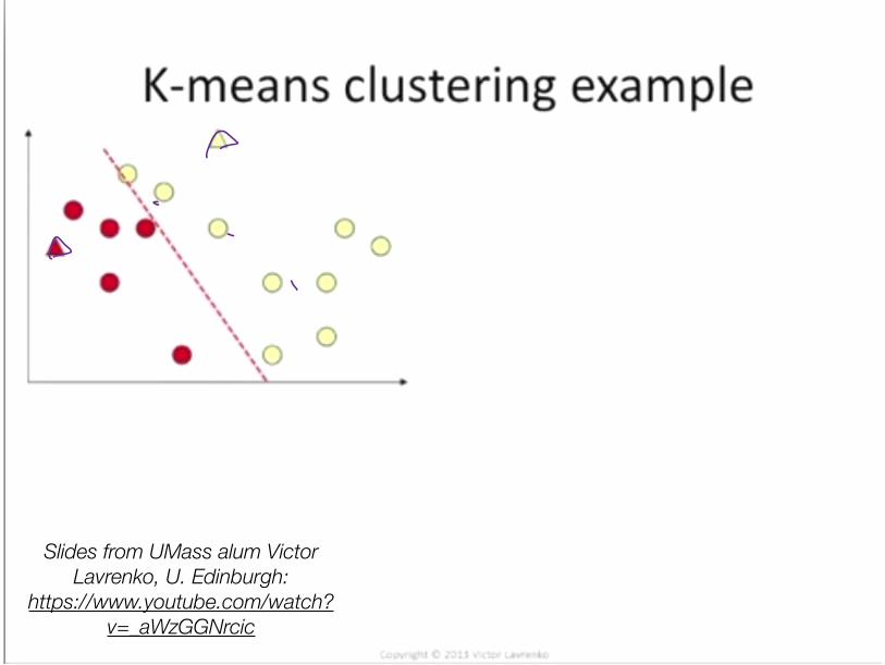
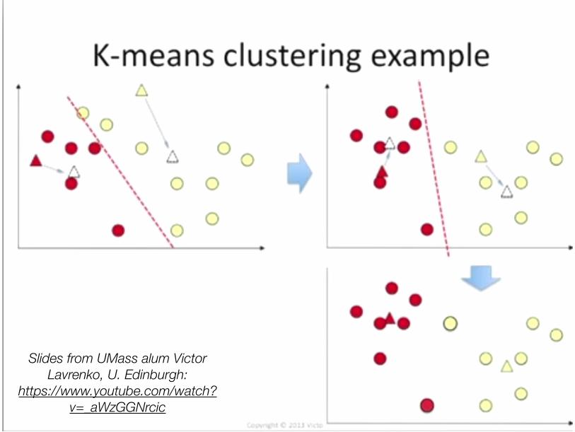
Slides from UMass alum Victor Lavrenko, U. Edinburgh:
https://www.youtube.com/watch?v=_aWzGGNrcic
8D
10
Slides from UMass alum Victor Lavrenko, U. Edinburgh:
https://www.youtube.com/watch?v=_aWzGGNrcic
sa

11
Slides from UMass alum Victor Lavrenko, U. Edinburgh:
https://www.youtube.com/watch?v=_aWzGGNrcic
i
so
Eady
12
Slides from UMass alum Victor Lavrenko, U. Edinburgh:
https://www.youtube.com/watch?v=_aWzGGNrcic
doI
13
Slides from UMass alum Victor Lavrenko, U. Edinburgh:
https://www.youtube.com/watch?v=_aWzGGNrcic
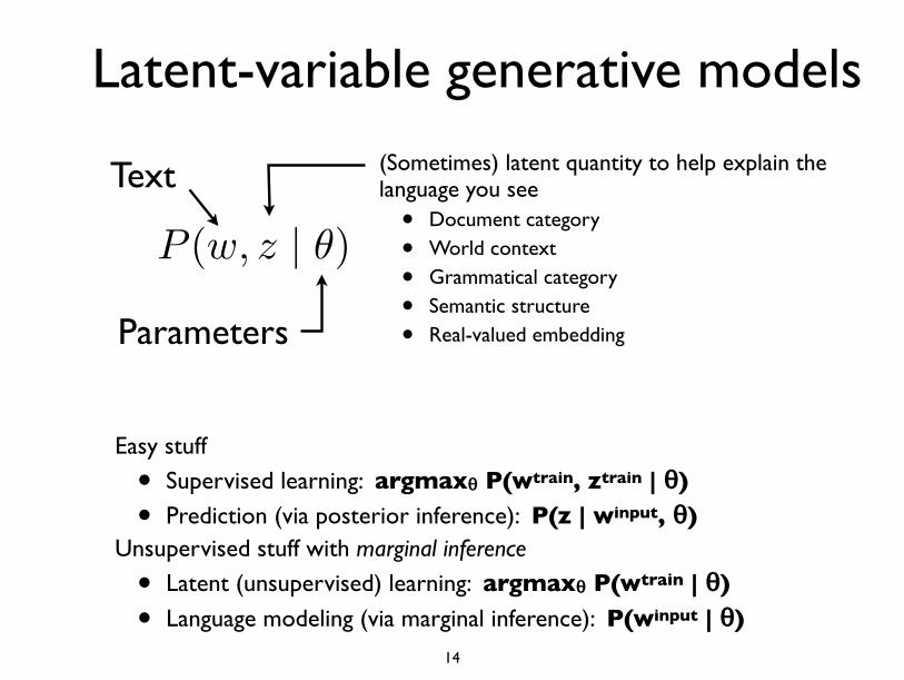
Latent-variable generative models
14
Text (Sometimes) latent quantity to help explain the language you see
• Document category
• World context
• Grammatical category
• Semantic structure
• Real-valued embedding
Easy stuff
• Supervised learning: argmaxθ P(wtrain, ztrain | θ)• Prediction (via posterior inference): P(z | winput, θ)
Unsupervised stuff with marginal inference
• Latent (unsupervised) learning: argmaxθ P(wtrain | θ)• Language modeling (via marginal inference): P(winput | θ)
P (w, z | ✓)
Parameters
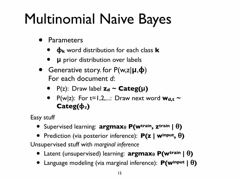
Multinomial Naive Bayes• Parameters
• ɸk word distribution for each class k• μ prior distribution over labels
• Generative story. for P(w,z|μ,ɸ) For each document d:
• P(z): Draw label zd ~ Categ(μ)• P(w|z): For t=1,2,...: Draw next word wd,t ~
Categ(ɸz)
15
Easy stuff
• Supervised learning: argmaxθ P(wtrain, ztrain | θ)• Prediction (via posterior inference): P(z | winput, θ)
Unsupervised stuff with marginal inference
• Latent (unsupervised) learning: argmaxθ P(wtrain | θ)• Language modeling (via marginal inference): P(winput | θ)
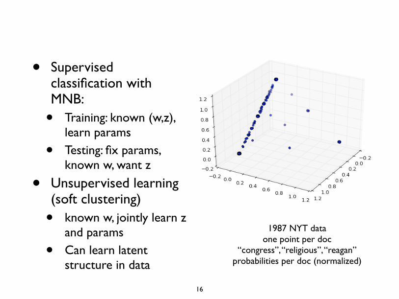
• Supervised classification with MNB:
• Training: known (w,z), learn params
• Testing: fix params, known w, want z
• Unsupervised learning (soft clustering)
• known w, jointly learn z and params
• Can learn latent structure in data
16
1987 NYT dataone point per doc
“congress”, “religious”, “reagan”probabilities per doc (normalized)
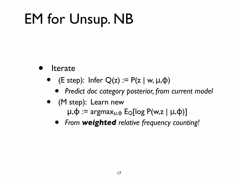
EM for Unsup. NB
• Iterate
• (E step): Infer Q(z) := P(z | w, μ,ɸ)
• Predict doc category posterior, from current model
• (M step): Learn new μ,ɸ := argmaxμ,ɸ EQ[log P(w,z | μ,ɸ)]
• From weighted relative frequency counting!
17
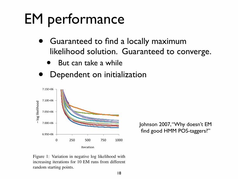
EM performance
• Guaranteed to find a locally maximum likelihood solution. Guaranteed to converge.
• But can take a while
• Dependent on initialization
18
Johnson 2007, “Why doesn’t EM find good HMM POS-taggers?”
H(T |Y ) = H(T )� I(Y, T )VI (Y, T ) = H(Y |T ) + H(T |Y )
As Meila (2003) shows, VI is a metric on the spaceof probability distributions whose value reflects thedivergence between the two distributions, and onlytakes the value zero when the two distributions areidentical.
3 Maximum Likelihood viaExpectation-Maximization
There are several excellent textbook presentations ofHidden Markov Models and the Forward-Backwardalgorithm for Expectation-Maximization (Jelinek,1997; Manning and Schutze, 1999; Bishop, 2006),so we do not cover them in detail here. Conceptu-ally, a Hidden Markov Model generates a sequenceof observations x = (x0, . . . , xn) (here, the wordsof the corpus) by first using a Markov model to gen-erate a sequence of hidden states y = (y0, . . . , yn)(which will be mapped to POS tags during evalua-tion as described above) and then generating eachword xi conditioned on its corresponding state yi.We insert endmarkers at the beginning and endingof the corpus and between sentence boundaries, andconstrain the estimator to associate endmarkers witha state that never appears with any other observationtype (this means each sentence can be processed in-dependently by first-order HMMs; these endmarkersare ignored during evaluation).
In more detail, the HMM is specified by multi-nomials �y and �y for each hidden state y, where�y specifies the distribution over states following yand �y specifies the distribution over observations xgiven state y.
yi | yi�1 = y � Multi(�y)xi | yi = y � Multi(�y)
(1)
We used the Forward-Backward algorithm to per-form Expectation-Maximization, which is a proce-dure that iteratively re-estimates the model param-eters (�, �), converging on a local maximum of thelikelihood. Specifically, if the parameter estimate attime � is (�(�),�(�)), then the re-estimated parame-ters at time � + 1 are:
�(�+1)y�|y = E[ny�,y]/E[ny] (2)
�(�+1)x|y = E[nx,y]/E[ny]
6.95E+06
7.00E+06
7.05E+06
7.10E+06
7.15E+06
0 250 500 750 1000
–lo
g lik
elih
ood
Iteration
Figure 1: Variation in negative log likelihood withincreasing iterations for 10 EM runs from differentrandom starting points.
where nx,y is the number of times observation x oc-curs with state y, ny�,y is the number of times statey� follows y and ny is the number of occurences ofstate y; all expectations are taken with respect to themodel (�(�),�(�)).
We took care to implement this and the other al-gorithms used in this paper efficiently, since optimalperformance was often only achieved after severalhundred iterations. It is well-known that EM oftentakes a large number of iterations to converge in like-lihood, and we found this here too, as shown in Fig-ure 1. As that figure makes clear, likelihood is stillincreasing after several hundred iterations.
Perhaps more surprisingly, we often found dra-matic changes in accuracy in the order of 5% occur-ing after several hundred iterations, so we ran 1,000iterations of EM in all of the experiments describedhere; each run took approximately 2.5 days compu-tation on a 3.6GHz Pentium 4. It’s well-known thataccuracy often decreases after the first few EM it-erations (which we also observed); however in ourexperiments we found that performance improvesagain after 100 iterations and continues improvingroughly monotonically. Figure 2 shows how 1-to-1accuracy varies with iteration during 10 runs fromdifferent random starting points. Note that 1-to-1accuracy at termination ranges from 0.38 to 0.45; aspread of 0.07.
We obtained a dramatic speedup by working di-rectly with probabilities and rescaling after each ob-servation to avoid underflow, rather than workingwith log probabilities (thanks to Yoshimasa Tsu-
298
EM pros/cons• Works best for a simple model with rapid E/M-step
inference - like Naive Bayes
• Requires probabilistic modeling assumptions
• Dependent on initialization
• Many alternative methods (e.g. MCMC), but can similar issues with local optima
• EM used for lots in NLP, esp. historically
• Machine translation
• HMM-based speech recognition
• Topic modeling, doc clustering
• At the moment, gradient-based learning for non-probabilistic models (vanilla NNs or matrix factorization) is more common. Note EM and prob. models can be mixed with neural networks (cutting edge research area).
19


![Statistical NLP Winter 2008 Lecture 16: Unsupervised Learning I Roger Levy [thanks to Sharon Goldwater for many slides]](https://img.pdfslide.net/doc/110x75/56649eb15503460f94bb6eaf/statistical-nlp-winter-2008-lecture-16-unsupervised-learning-i-roger-levy.jpg)